Undergraduate Research Opportunity

Programme in Science

A Mathematical Supplement To

“The Sun in the Church: Cathedrals as Solar Observatories”

by J.L. Heilbron

NG YOKE LENG

SUPERVISOR ASSOC. PROF. HELMER ASLAKSEN

Department of Mathematics

National University of Singapore

Semester II, 2000/2001

2

INTRODUCTION J.L. Heilbron’s book “The Sun in the Church” addresses a basic problem: how is time

measured? Since the time period of the Earth’s orbit around the Sun is not neatly

divisible into a whole number of days, it is hard to construct a calendar that will mark

a moment in time back at the exact same point after the Earth makes a complete orbit

around the Sun. In the book, Heilbron gives a comprehensive overview of the various

approaches that have been proposed and implemented by the Catholic Church to fix

the calendar. As the Church wanted to have a systematic way to determine when

Easter should be celebrated, the calendar had to be made as accurate and reliable as

possible. In consequence, the Church became deeply involved in improving the

quality of observational data on which calendars were based. Huge cathedrals were

considered to be ideal solar observatories: by making a hole in the ceiling and fixing a

mark on the floor where the sun's shadow fell along a meridiana, or a line laid out on

the cathedral floor, exact measurements could be made regarding the position of the

sun.

Many historical and technical facts on how the cathedrals came to be used as

an instrument of measurement have been recorded in this book. Heilbron has

succeeded in providing the readers with a most enriching and interesting experience

as they read the historical account. Nonetheless, most readers would probably find it

hard to appreciate the technical sections of this book because these sections call for a

certain level of understanding in some mathematical concepts. This paper has been

specially written as a mathematical supplement to enable readers to have a clearer

comprehension of how certain conclusions have been drawn or how certain values

have been obtained. Due to the sheer volume of this book, the supplement provides

explanations for only a few sections of it; similar supplements for the rest of the book

are expected to appear in the near future.

The structure of this supplement is broadly categorized into two parts. Firstly,

a collection of preliminary information used in later explanations is given. This

includes some mathematical tools and the models created by Hipparchus, Ptolemy and

Kepler to explain the motions of the Sun and the planets. Secondly, detailed

explanations of selected sections of Heilbron’s book are provided. These concern the

steps in calculation involved in working out certain values and the comparison of

3

models. The use of a meridiana to justify the superiority of one model over another is

also discussed.

1. Preliminaries

1.1 Background of various mathematicians mentioned

This section aims to provide more information on the prominent

mathematicians mentioned in this paper so that readers may have a more

defined impression of their names as they read this paper. The primary source

for the contents of this section is:

http://www-groups.dcs.st-andrews.ac.uk/~history/Mathematicians/ .

1.1.1 Hipparchus

Little is known of Hipparchus’ life, but he is known to have been born

in Nicaea in Bithynia. The town of Nicaea is now called Iznik and is

situated in north-western Turkey. Despite being a mathematician and

astronomer of great importance, Hipparchus’ work has not been well

documented; only one work of his has survived, namely Commentary

on Aratus and Eudoxus. Most of his discoveries have been made

known to us only through Ptolemy’s Almagest. His contributions to the

field of mathematics include producing a trigonometric table of chords,

introducing the division of a circle into 360 o into Greece, calculating

the length of the year within 6.5'and discovering precession of the

equinoxes.

1.1.2 Claudius Ptolemy

One of the most influential Greek astronomers and geographers of his

time, Ptolemy propounded the geocentric theory in a form that

prevailed for 1400 years. We do not know much about his life but most

of his major works have survived. His earliest and most important

piece is the Almagest which gives in detail the mathematical theory of

the motions of the Sun, Moon and planets. This thirteen-book treatise

was not superseded until a century after another mathematician,

4

Copernicus, presented his heliocentric theory in the De revolutionibus

of 1543.

1.1.3 Johannes Kepler

Born in the small town of Weil der Stadt in Swabia and moved to

nearby Leonberg with his parents in 1576, Kepler is now chiefly

remembered for discovering the three laws of planetary motion that

bear his name published in 1609 and 1619. As much of his

correspondence survived, we know a significant amount of Kepler’s

life and character. He did important work in optics, discovered two

new regular polyhedra, gave the first mathematical treatment of close

packing of equal spheres which led to an explanation of the shape of

the cells of a honeycomb, gave the first proof of how logarithms

worked and devised a method of finding the volumes of solids of

revolution that can be seen as contributing to the development of

calculus. Moreover, he calculated the most exact astronomical tables

then known, whose continued accuracy did much to establish the truth

of heliocentric astronomy.

1.1.4 Giovanni Cassini

Cassini studied at the Jesuit college in Genoa and then at the abbey of

San Fructuoso. He observed at Panzano Observatory between 1648 and

1669 and in 1650, became professor of astronomy at the University of

Bologna. Aside from an interest in astronomy, Cassini was also an

expert in hydraulics and engineering. He was later employed by the

Pope to oversee fortifications and river management on the river Po. In

1669, the senate of Bologna granted him approval to visit Paris under

the invitation of Louis XIV, thinking that the trip would be a short one;

yet he never returned to Italy. He became director of the Paris

Observatory in 1671 and then switched to French citizenship two years

later.

5

1.2 Some Mathematical Tools

1.2.1 Ellipses

Many mathematical textbooks contain comprehensive accounts of

what an ellipse is and what its properties are. A recommended

reference text is “Basic Calculus: from Archimedes to Newton to its

Role in Science” written by Alexander J Hahn, and in particular, pages

54 – 55 and 90 – 94.

Here, some of the properties have been selected and stated below for

easy reference.

Figure 1

With reference to Figure 1, the standard equation of the ellipse is

2 2

2 2 1.x y

a b+ =

Since the point ( )0,B b= is on the ellipse, 1 1 22 2 ,BF BF BF a= + = and

hence 1 .BF a= Similarly, 2 .BF a= By Pythagoras’ Theorem,

2 2 2

2 2 2 2

2 2 2 2

2 2 2

( )

(1 ).

a b ae

a b a e

b a a e

b a e

= +

= +

= −

= −

In addition, eccentricity is defined as the ratio of the distance between

the centre of the ellipse and one of the foci to the semimajor axis, or

eccentricity = .ae

ea

=

6

Figure 2

Referring to Figure 2, Cavalieri’s Principle states that if x xd kc= for

all x and for a fixed positive number k, then D = kC.1

Now, consider simultaneously the graph of the ellipse 2 2

2 2 1x ya b

+ = and

that of the circle 2 2 2 ,x y a+ = as shown in Figure 3.

Figure 3

Let x satisfy a x a− ≤ ≤ and, let ( ),x y and ( )0,x y be the indicated

points on the ellipse and circle, respectively. Since ( )0,x y satisfies

2 2 2x y a+ = and 0 0,y ≥ it follows that 2 20 .y a x= −

Since ( ),x y is on the ellipse,

1 Hahn, pg 93.

7

( )

2 2 2 2

2 2 2

2 2 2 2 22 2 2

2 2

2 20

1

.

y x a xb a a

b a b x by a x

a ab b

y a x ya a

−= − =

−= = −

= − =

The above relation is frequently used in later calculations. In addition,

if we suppose that the upper semicircles and the upper part of the

ellipse are separated as shown in Fig. 4(a), we would then have

demonstrated that x xd kc= for all x.

Figure 4

Since the area of a semicircle of radius a is 21

2aπ , it follows by

Cavelieri’s principle that the area of the upper half of the ellipse is

equal to 21 12 2

ba ab

aπ π =

. Therefore, the full ellipse with semimajor

axis a and semiminor axis b has area abπ . Note that Cavalieri’s

principle also applies to Figure 4(b). In particular, the area of the

elliptical section has area ba

times that of the semicircular section.

1.2.2 Small-angle approximations

Some angles dealt with in astronomy are small and may be

approximated with little error caused. Consider θ being a small angle.

8

The Maclaurin series or Taylor series about the origin for sinθ , cosθ

and tanθ up to terms in 2θ are recorded below.

2

sin

cos 12

tan .

θ θ

θθ

θ θ

≈

≈ −

≈

1.2.3 Binomial Theorem

The Binomial Theorem states that for every pair of real numbers x and

y and every natural number n,

1 1( 1)...( 1)( ) ... ... .

!n n n n k k n nn n n k

x y x nx y x y nxy yk

− − −− − ++ = + + + + + +

1.2.4 Point of view

The fact that the dimensions of our planetary system are so minute in

comparison with the distances to the fixed stars, which form the

background of the celestial sphere, causes little observable error if

either the Sun or the Earth is kept in a fixed position with respect to the

surrounding universe. In this section, we investigate the apparent

motion of the Sun, as well as that of the planets, when viewed from a

fixed Earth. The former is based on page 118 of “The Exact Sciences

in Antiquity” by O. Neugebauer whilst the latter is based on page 1010

of James Evans’ article entitled “The division of the Martian

eccentricity from Hipparchos to Kepler: A history of the

approximations to Kepler motion”.

Consider a system with only Sun S and Earth E. We know that

the Earth revolves around the Sun and completes its orbit in a year. See

Figure 5(a).

Figure 5

9

By arresting the motion of the Earth, we would also observe the Sun to

revolve around Earth on a circular path but in the opposite direction.

This is shown in Figure 5(b). The apparent path of the Sun around the

Earth is called the ecliptic.

Now, consider the motion of a superior planet, or one that is

farther than the Earth with respect to the Sun, on a heliocentric theory.

Figure 6

With reference to Figure 6(a), the Earth E executes an orbit, not

necessarily circular, about the stationary Sun S. In the course of a year,

the position vector SEuuv

rotates anticlockwise about S. The angular

speed of SEuuv

varies slightly in the course of the year, and so does the

length of the vector. Similarly, a superior planet Z revolves around the

Sun in a larger orbit. Vector SZuuv

varies at its own slightly different

rate. At any instant, the line of sight from the Earth to the planet

coincides with EZuuuv

which is also equal to .SE SZ− +uuv uuv

Since these

vectors may be added in either order, EZuuuv

is also equivalent to

( ).SZ SE+ −uuv uuv

The new form of the addition is shown in Figure 6(b).

Here we begin at the Earth E. A vector equal toSZuuv

is drawn

with its tail at E; let the head of this vector be called K. ThenEKuuuv

rotates in Figure 6(b) at the same rate as SZuuv

rotates in Figure 6(a). At

K, place the tail of a second vector, equal to ,SE−uuv

with its head at

planet Z. This series of steps brings about a transformation in a

superiors planet from a heliocentric model (Figure 6(a)) to a geocentric

model (Figure 6(b)). Point K serves as the centre of a small circle, or

an epicycle, upon which Z revolves while K itself moves on a large

10

carrying circle, or deferent, about the Earth E. The equivalence of

Figures 6(a) and 6(b) is a consequence of the commutative property of

vector addition. Hence, in the case of a superior planet, the epicycle

corresponds to the orbit of the Earth about the Sun, and the deferent, to

the heliocentric orbit of the planet itself.

In the case of an inferior planet, or one that is between the Sun

and the Earth in the planetary system, the transformation is similar to

that as explained for superior planets, but with adjustments made to the

vectors and vector addition.

Figure 7

With reference to figures 7(a) and 7(b), S, E and Z retain their

original representations. Notice in Figure 7(a), however, that Z is on

the inner orbit and vector EZuuuv

is equal to .SE SZ− +uuv uuv

We draw a vector

equivalent to SE−uuv

with its tail at E and its head at a new point called

K on the deferent. At K, we add a vector equal to SZuuv

and call it .KZuuuv

Once again, Figures 7(a) and 7(b) are equivalent to each other because

of the commutative property of vector addition. Thus, for an inferior

planet, the epicycle corresponds to its heliocentric orbit whilst the

deferent corresponds to the orbit of the Earth about the Sun.

1.3 Hipparchus’ model of the motion of the Sun

Greek astronomers believe that all orbits of luminaries and planets

treated in astronomy should be circles or components of circles.2 The simplest

manner to represent the apparent motion of the Sun S as observed from the

Earth E would be a circle in the plane of the ecliptic, centered on the Earth E.

This may be seen in Figure 8.

2 Heilbron, pg 103.

11

Figure 8

The solstices and equinoxes are located 90ο apart as seen from the

Earth E, and if we take y as the number of days in a year, we would expect the

interval between the seasons to be exactly of length 4y

days. However, the

observed facts show otherwise: the seasons are not equal.3 In particular,

Hipparchus found the Sun to move 90o in the ecliptic plane from Spring

equinox to Summer solstice in 94½ days and 90o from Summer solstice to

Autumn equinox in 92½ days.4 Modern values for the lengths of the seasons

are as follows: Spring – 92 days, 18 hours, 20 minutes or 92.764 days;

Summer – 93 days, 15 hours, 31 minutes or 93.647 days; Autumn – 89 days,

20 hours, 4 minutes or 89.836 days; and Winter – 88 days, 23 hours, 56

minutes or 88.997 days.5 To explain this phenomenon, ancient astronomers

would rather regard the inequalities in the speed of the Sun as an optical

illusion than rule that the Sun does not move at uniform angular speed. For

more information on how the illusion works, please refer to pages 104 – 105

in Heilbron’s book. The essence of their solution was to displace the Earth

from the centre of the Sun’s orbit.

3 Heilbron, pg 103. 4 Hoskin, pg 41. 5 Hahn, pg 41.

12

Figure 9

Much of the information in this paragraph concerning Hipparchus’

simple model of the orbit of the Sun is quoted from page 41 of “The

Cambridge Illustrated of Astronomy” by Michael Hoskin. In Figure 9,

Hipparchus’ solar model is given. The Earth is stationary at E, while the Sun S

moves around the circle at a uniform angular speed about the centre of the

circle C. The Sun’s circle is thus said to be eccentric to the Earth. To generate

the longer intervals between solstice and equinox, the Earth had to be removed

from the centre in the opposite direction so that the corresponding arcs as seen

from the Earth would each be more than 14

of the circle, and it would take

longer than 4y

days to traverse them. Hipparchus’ calculations showed that

the distance between the Earth and centre has to be 1/24 of the radius of the

circle and that the line from the Earth to centre had to make an angle of 65½ o

with the Spring equinox.

At this point, I would like to highlight some of the terminology used in

Heilbron’s book as well as this paper.

13

Figure 10

With reference to Figure 10, suppose a is the radius of the circle centered at C

and Z is a body moving on the circle. The eccentricity e is defined as the ratio

of the distance between O and C to radius a, that is,

/ .e OC a=

This is similar to the definition of eccentricity for an ellipse. In Hipparchus’

model for the Sun’s orbit mentioned earlier, the figure “1/24” is in fact the

eccentricity. The distance of separation OC is thus equivalent to ae.

Perigee Π occurs where Z is closest to O whilst apogee A occurs where Z is

furthest from O.

The line joining the perigee and apogee is known as the line of apsides or

“the diameter of the Sun’s orbit that runs through the centre of the ecliptic”.6

1.4 Ptolemy’s solar and planetary models

Ptolemy’s solar model is equivalent to that of Hipparchus’ and thus, is not

repeated here. In Heilbron’s book, Ptolemy’s method for obtaining the solar

eccentricity and the angle between the line of apsides and the line joining the

solstices ψ is illustrated and explained; the calculations involved are provided

in Section 2.1 of this paper. When modern values for time differences between

solstice and equinox are applied to Ptolemy’s model, the value found for the

angle ψ is fairly close to that found in the past. However the same could not be

said for the value of eccentricity. In fact, the old value for solar eccentricity e

exceeds the modern value by a factor of two. More discussion on this issue is

provided later in this section.

6 Heilbron, pg 104.

14

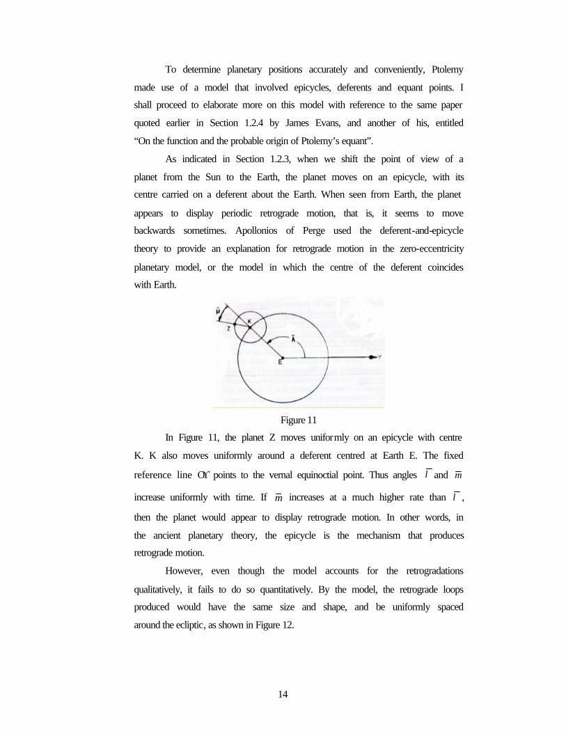
To determine planetary positions accurately and conveniently, Ptolemy

made use of a model that involved epicycles, deferents and equant points. I

shall proceed to elaborate more on this model with reference to the same paper

quoted earlier in Section 1.2.4 by James Evans, and another of his, entitled

“On the function and the probable origin of Ptolemy’s equant”.

As indicated in Section 1.2.3, when we shift the point of view of a

planet from the Sun to the Earth, the planet moves on an epicycle, with its

centre carried on a deferent about the Earth. When seen from Earth, the planet

appears to display periodic retrograde motion, that is, it seems to move

backwards sometimes. Apollonios of Perge used the deferent-and-epicycle

theory to provide an explanation for retrograde motion in the zero-eccentricity

planetary model, or the model in which the centre of the deferent coincides

with Earth.

Figure 11

In Figure 11, the planet Z moves uniformly on an epicycle with centre

K. K also moves uniformly around a deferent centred at Earth E. The fixed

reference line Oϒ points to the vernal equinoctial point. Thus angles λ and µ

increase uniformly with time. If µ increases at a much higher rate than λ ,

then the planet would appear to display retrograde motion. In other words, in

the ancient planetary theory, the epicycle is the mechanism that produces

retrograde motion.

However, even though the model accounts for the retrogradations

qualitatively, it fails to do so quantitatively. By the model, the retrograde loops

produced would have the same size and shape, and be uniformly spaced

around the ecliptic, as shown in Figure 12.

15

Figure 12

Yet this is overly simplified and does not occur in reality. The precise distance

between one retrogradation and the next is quite variable, and thus the

retrograde arcs are not equally spaced around the zodiac. There is no way for

the uniformly spaced retrograde loops of the model to reproduce the unevenly

spaced retrograde arcs of the planet itself.

A step taken to improve this zero-eccentricity model was to displace

the Earth E from the centre of the deferent, C, slightly.

Figure 13

In Figure 13, planet Z moves uniformly on the epicycle and the centre

of the epicycle, K, moves around the deferent at uniform speed. However, C

no longer coincides with E, as in the “zero-eccentricity model”. This is known

as the “intermediate model”. The intermediate model provided just the kind of

variable spacing between two retrogradations of the planet yet it was still

unable to fit the width of the retrograde loops perfectly. To tackle the problem,

Ptolemy added a third device called the equant point, defined as a point about

which the angular velocity of a body on its orbit is seen as constant. Figure 14

shows Ptolemy’s planetary model.

16

Figure 14

Here, Z, K and E retain their usual representations. However K is now

assumed not to move uniform either with respect to the Earth E or the centre

of the deferent, C. Instead, uniform motion of K is observed at X which is the

mirror image of the Earth E, and is what Ptolemy named as the “equant point”.

As a result of these two points X and E, there are now two

eccentricities to be defined. Take the radius of the deferent to be a, the

eccentricity of the Earth E with respect to centre C to be 1e and the

eccentricity of the equant point with respect to centre C to be 2e . Then,

1

2

/ ,

/ .

e EC a

e XC a

==

The rule of equant motion – that K moves at constant angular speed as viewed

from the equant – produces a physical variation in the speed of K. This

variation in speed is determined by 2e and if 2e goes to zero, the motion of K

reduces to uniform circular motion. Even if 2e were zero, the eccentricity 1e

would cause the motion of K to appear non-uniform from the Earth E due to

the same optical illusion mentioned in Section 1.2. The sum 1 2e e+ is called

the “total eccentricity”. Ptolemy always puts 1 2e e= and such a situation has

come to be referred to as the “bisection of eccentricity”. This notion would

once again be brought up in Section 2.2 where we make comparisons across

Hipparchus’, Ptolemy’s and Kepler’s solar and planetary models.

1.5 Kepler’s laws

After a tedious and difficult research process, Kepler found enough

evidence that proved the planetary theories advocated by Copernicus and

Ptolemy false. Instead, he discovered three laws that could describe how the

17

planets move with reference to the Sun with more precision. The following

information is based on pages 98 – 99 and 111 – 114 of “Text-Book on

Spherical Astronomy, Fourth Edition” written by W.M. Smart.

Kepler’s First Law states that the path, or orbit, of a planet around the Sun is

an ellipse, the position of the Sun being at a focus of the ellipse.

Figure 15

Figure 15 above shows an ellipse of which S and F are the two foci, C

is the centre (midway between S and F) and ΠA is the major axis. The Sun

will be supposed to be at S and the planet to move round the ellipse in the

direction of the arrows. At Π , the planet is at perigee, whilst at A, it is at

apogee. ΠC is the semimajor axis; its length is given by a. DC is the

semiminor axis; its length is denoted by b. The eccentricity e is given by the

ratio SC : SA. Just as highlighted in Section 1.2.1, 2 2 2(1 )b a e= − . The perigee

distance SΠ is (1 )a e− and apogee distance SA is (1 )a e+ .

Let ρ denote the distance of the planet Z from the Sun and the angle θ

be the planet’s angular distance from perigee, or the true anomaly. The

equation of its elliptical orbit is known to be

2 2(1 )1 cos 1 cos

b a a ee e

ρθ θ

−= =+ +

The time required for the planet to describe its orbit is called the

period, denoted by T. In time T, the radius vector SZ sweeps out an angle of

2π and thus, the mean angular velocity of the planet, w, is 2

T

π.

18

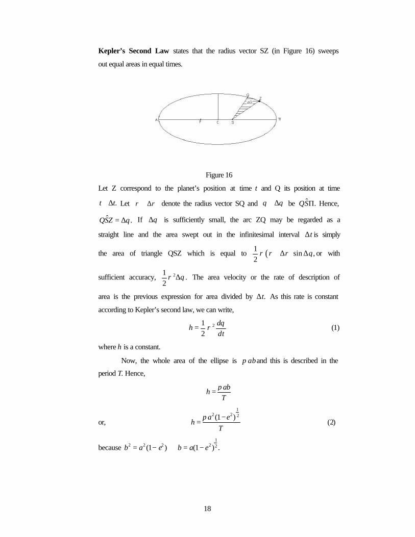
Kepler’s Second Law states that the radius vector SZ (in Figure 16) sweeps

out equal areas in equal times.

Figure 16

Let Z correspond to the planet’s position at time t and Q its position at time

.t t+ ∆ Let ρ ρ+ ∆ denote the radius vector SQ and θ θ+ ∆ be ˆ .QSΠ Hence,

ˆ .QSZ θ= ∆ If θ∆ is sufficiently small, the arc ZQ may be regarded as a

straight line and the area swept out in the infinitesimal interval t∆ is simply

the area of triangle QSZ which is equal to ( )1sin ,

2ρ ρ ρ θ+ ∆ ∆ or with

sufficient accuracy, 21.

2ρ θ∆ The area velocity or the rate of description of

area is the previous expression for area divided by .t∆ As this rate is constant

according to Kepler’s second law, we can write,

212

dh

dtθρ= (1)

where h is a constant.

Now, the whole area of the ellipse is abπ and this is described in the

period T. Hence,

abh

Tπ=

or,

12 2 2(1 )a e

hT

π −= (2)

because 1

2 2 2 2 2(1 ) (1 ) .b a e b a e= − ⇒ = −

19

By (1) and (2), we have,

12 2 2

21 (1 ).

2d a edt Tθ πρ −=

Figure17

Theoretically, if the values of the semimajor axis a, the eccentricity e,

the time at which the planet passed through perigee τ and the orbital period T

are known, Kepler’s second law would enable us to determine the position of

the planet in its orbit at any instant.

Referring to Figure 17, Z is the position of the planet at time t. In the

interval (t - τ) the radius vector moving from SΠ to SZ sweeps out the shaded

area SZΠ. By Kepler’s Second Law,

Area SZΠ : Area of ellipse = t - τ : T.

Hence, Area SZΠ = ( )

,ab t

T

π τ−

Or, Area SZΠ = 1

( )2

wab t τ−

where w = 2Tπ

and 2 2 2(1 )b a e= − .

This method may seem easy but in practice, it is inconvenient; the

alternative is explained in detail in Section 2.4.

20

2. Selected sections

2.1 Notes to Heilbron, pg 105: Ptolemy’s method of obtaining the solar

eccentricity

Figure 18

As highlighted in Section 1.2.4, Ptolemy made use of Hipparchus’

model for the Sun’s motion around the earth and calculated values for the

solar eccentricity, e, and the angle ψ between the line of apsides and the line

joining the solstices. Figure 13 shows the model that Ptolemy used to work out

the aforesaid values and this section aims to provide a detailed set of working

to obtain the result quoted at the end of the page: e = 0.0334, ψ = 1258'o , by

applying modern seasonal lengths.

Since fall is longer than spring, EA must point somewhere between the

summer solstice and autumnal equinox. By doing so, when viewed from the

earth, the sun’s orbit between points I and J would be longer than 14

arc of the

entire path. Then consequently, EΠ points between the winter solstice and the

spring equinox. Taking the Julian value for the number of days in a year

(denoted by y), the mean angular motion of the sun, w, is equal to 360 / yo per

day, or

360 /365.25 0.9856w = ≈o o per day

Given that the differences in time between the sun’s arrival at G, H, I and J on

its orbit, when, viewed from the earth E, as it appears at the first points of

Aries, Cancer, Libra and Capricorn, respectively are 89d0h, 92d18h, 93d15h,

89d20h, and, we work out the following angles:

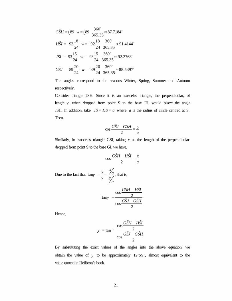
21

( ) ( ) 360ˆ 89 89 87.7184365.35

18 18 360ˆ 92 92 91.414424 24 365.35

15 15 360ˆ 93 93 92.276824 24 365.35

20 20 360ˆ 89 89 88.539724 24 365.35

GSH w

HSI w

JSI w

GSJ w

= = ≈

= = ≈ = = ≈ = = ≈

oo

oo

oo

oo

The angles correspond to the seasons Winter, Spring, Summer and Autumn

respectively.

Consider triangle JSH. Since it is an isosceles triangle, the perpendicular, of

length y, when dropped from point S to the base JH, would bisect the angle

JSH. In addition, take JS HS a= = where a is the radius of circle centred at S.

Then,

ˆ ˆcos

2GSJ GSH y

a+ =

Similarly, in isosceles triangle GSI, taking x as the length of the perpendicular

dropped from point S to the base GI, we have,

ˆ ˆcos

2GSH HSI x

a+ =

Due to the fact that tanxx ayy

a

ψ = = , that is,

ˆ ˆcos

2tan ˆ ˆcos

2

GSH HSI

GSJ GSHψ

+

=+

Hence,

1

ˆ ˆcos

2tanˆ ˆ

cos2

GSH HSI

GSJ GSHψ −

+ =

+

By substituting the exact values of the angles into the above equation, we

obtain the value of ψ to be approximately 12 59 'o , almost equivalent to the

value quoted in Heilbron’s book.

22

To work out the value of eccentricity, e, we note that .ES

ea

= But

sin .sin

x xES

ESψ

ψ= ⇒ = Therefore, sin

.sin

x xae

aψ

ψ= = Using the result from

above, we have,

ˆ ˆcos

2sin

GSH HSI

eψ

+

=

After substituting the relevant values into the above relation, we obtain the

value of e to be around 0.0335, which is also close to that quoted in the book.

However, Ptolemy’s value of solar eccentricity which is 0.0334

exceeded that found by Kepler which is 0.0167. To account for this factor-of-

two difference, we have to look into the way in which Ptolemy and Kepler

measured the separation between the centre of the sun’s orbit and the earth.

Figure 19 provides a visual aid to this explanation.

Figure 19

C represents the centre of the sun’s orbit, EP denotes where Ptolemy

positions the earth, EK denotes where Kepler positions the earth and XK marks

Kepler’s equant point. Consider radius of the sun’s orbit to be a, then the

intervals between XK, C, EK and EP would each be 2

ae. Ptolemy calculated

eccentricity as 2 2Pae aeCE

ea a

+= = whereas Kepler calculated the same

quantity as 2 .2

KaeCE e

a a= = Thus, the factor-of-two difference is produced.

23

Even though we know now that Kepler’s model is the accurate one, it

would be interesting to find out how Ptolemy’s model had provided such a

close approximate to Kepler’s model. Since both models gave near similar

observations, mathematicians and astronomers alike had to struggle with

deciding which of the models was the correct one until the development of the

meridiana. In fact, the use of the meridiana to make measurements that would

allow substantial conclusions to be drawn from them is another area worth

exploring into. In the following sections of the paper, the discussion would

focus on the comparison of models and the use of the meridiana.

24

2.2 Comparing solar and planetary models

In this paper, three sets of solar and planetary models have been brought into

discussion, namely, by Hipparchus, Ptolemy and Kepler. Ptolemy’s equant

theory for the planets is an amazingly close approximate to Kepler’s planetary

model. In this section, we aim to find out mathematically how this has been

possible. Prior to that, we would derive the equations defining the position of a

body in its orbit in each of the three models. The defining parameters of the

body’s position are the true anomaly and the radius vector. In finding out the

equations of these parameters, we would also make use of the eccentricity.

Information on which this section is based mostly on Evans’ article entitled

“The division of the Martian eccentricity from Hipparchos to Kepler: A

history of the approximations to Kepler motion” and shall be complemented

with brief notes from other books as recorded in the reference section.

As described in Section 1.5, the equation for the elliptical orbit is

2(1 )

1 cos

a e

eρ

θ−

=+

(1)

where ρ is the planet’s distance from the Sun, θ is the true anomaly and e is

the eccentricity.

By means of the binomial theorem, the above equation may be expanded as

the following:

2 2( ) (1 cos sin ...)a e eρ θ θ θ= − − + (2)

Also derived in section 1.5 is the condition of constant areal velocity, that is,

12 2 2

21 (1 ).

2

d a e

dt T

θ πρ

−=

When (1) is substituted into the above, and the resulting differential equation

for ( )tθ is expanded and integrated through order e2, we obtain

25( ) 2 sin sin2 ,

4t wt e wt e wtθ = + + (3)

where w is the angular velocity.

Equations (2) and (3) are the defining equations for a body on the Keplerian

model. We next derive similar equations for a body on an eccentric orbit with

equant. Figure 20 is the reference diagram for the derivation steps that follow.

25

Figure 20

The equation of the orbit in polar coordinates for Z is that of a circle

eccentric to C, which is,

1

12 2 2

1( ) cos (1 sin )e eρ θ θ θ= − + −

Hence, by binomial theorem,

2 21 1

1( ) 1 cos sin

2e eρ θ θ θ≈ − − (4)

Since mean anomaly M is equivalent to wt and ,q M M qθ θ= − ⇒ = +

therefore, .wt qθ = +

Applying Sine Rule to triangle OZX, we have

1 2 1 2( )sinsin .

sin sin sin sinOX OZ e e e e wt

qq M q wt

ρρ

+ += ⇒ = ⇒ =

This gives 1 1 2( )sinsin

e e wtq

ρ− +=

.

Hence,

1 1 2( )sin( ) sin .

e e wtt wtθ

ρ− += +

By substituting the expression of ρ for an eccentric with equant model into

this equation, and expanding to second order in e, we get

1 2 1 1 2

1( ) ( )sin ( )sin2

2t wt e e wt e e e wtθ = + + + + (5)

26

For Hipparchus’ solar theory or perspectival theory, 1 2e e= and 2 0.e =

On Ptolemy’s equant theory, he does a bisection of eccentricity by putting 1 2 .e e=

Hence each is of value e.

Thus by substituting the two sets of eccentricity values into equations (3) and (4), we

find the corresponding true anomaly and radius vector equations as shown below. In

addition, equations (2) (include up to second order terms in e and set the semimajor

axis as unity) and (3) have also been added into the table for comparison purposes.

Model Eccentricities True anomaly Radius vector

Hipparchus 1e e= 22 sin 2 sin2wt e wt e wt+ + 2 21 2 cos 2 sine eθ θ− −

Ptolemy 1e e= and

2e e=

22 sin sin2wt e wt e wt+ + 2 211 cos sin

2e eθ θ− −

Kepler 1 2 2

ee e= = 25

2 sin sin24

wt e wt e wt+ + 2 21 cos sine eθ θ− −

Seeing the data, suppose we ignore the second order terms, then the first discrepancy

arises in the radius vector or Hipparchus’ model. Consider the true anomalies of

Ptolemy and Kepler. The difference between them is a mere 21sin2

4e wt which

amounts to a maximum of 8 min of arc. Considering the low level of precision in

instruments used to make measurements of celestial bodies in ancient days, it would

have been hard to recognize that this minute difference points towards an error in the

model. It is no wonder that so much controversy had occurred amongst the

astronomers then, in their desire to conclude which planetary theory was the true and

exact one. In fact, Ptolemy’s and Kepler’s models have approximated each other so

well that up to first order terms in e, the empty focus of the Keplerian ellipse is

indistinguishable form the equant point in Ptolemy’s model.

27

2.3 Use of meridiana and Notes to Appendix C

There has been a great controversy between adherents of Ptolemy’s

traditional solar theory and proponents of Kepler’s “bisection of the

eccentricity” in his solar model. This motivated Cassini to find out which

theory was the accurate one by using the meridiana at San Petronio; and he

succeeded. The basis of and working steps to his conclusion are elaborated in

this section.

As highlighted in Section 2.1, the modern value of the eccentricity is

half of the ancient. Suppose in Ptolemy’s model, the solar eccentricity is of

value e, then the same quantity would be of value 2e

in Kepler’s model.

(a) (b)

Figure 21

Referring to Figure 21(a), we see that at perigee, the distance between Sun and

Earth is shorter on Ptolemy’s model than that on Kepler’s. From 21(b), the

opposite occurs: at apogee, the same distance is longer on Ptolemy’s model

than that on Kepler’s. If the apsidal separation between Sun and Earth could

be observed directly, then it would be possible to test out which of the two

models is the correct one. Such a direct observation cannot be obtained but

fortunately, a convenient substitute exists in the Sun’s apparent diameter,

which is inversely proportional to its separation from the Earth.

Astronomers had found that the Sun’s apparent diameter at mean

distance ranges from 30'30'' to32'44''. In addition, the difference between

the Sun’s diameters at the absides was found to be either 1' or 2'. The table

below lists the apogee distance, perigee distance and absidal difference

between Sun and Earth corresponding to Kepler’s and Ptolemy’s theories, or

28

as Heilbron names them, equant theory, and pure eccentric or perspectival

theory respectively.

Theory by Apogee distance Perigee distance Absidal Difference

Kepler 1

2e

a + 1

2e

a −

ae

Ptolemy a(1 + e) a(1 – e) 2ae

Figure 22

In Figure 22, GH is of length 2s, OC refers to the separation between the Sun

and the Earth at the apsides. Let GO = HO = d. Since triangles GOC and HOC

are right-angled, by Pythagoras’ Theorem, d is equivalent to 2 2s OC+ .

Finally, β refers to half the apparent apsidal diameter of the Sun. Since β is

small, it may be approximated by sinβ. In the calculations that follow, the

subscripts Π and A, when attached to a certain quantity, mark the same

quantity as that measured at perigee and apogee respectively.

On the perspectival theory, 22

sin .s

s OCβ βΠ Π

Π

≈ =+

Since

(1 )OC a eΠ = − and s2 is negligibly small, 2 2 2

.(1 )(1 )

s sa es a e

βΠ = ≈−+ −

By

similar derivation, and using (1 ),AOC a e= + we obtain .(1 )A

sa e

β =+

29

The difference between the apsidal diameters is

2 2

2( )

2(1 ) (1 )

2 1 1,

1 1

A

A

s s

a e a e

sa e e

β β

β βΠ

Π

−= −

= − − +

= − − +

and considering up to terms in e only,

2[(1 ) (1 )]

42

se e

ase

ea

σ

≈ + − −

= =

where 2

.s

aσ =

Similarly, for the equant theory, by using 12e

OC aΠ = −

and

1 ,2A

eOC a = +

we get

2 2

21 1

2 2

2 1 1

1 12 2

21 1

2 2

2.

A

s se e

a a

se ea

s e ea

see

a

β β

σ

Π −

= −

− +

= − − + ≈ + − −

= =

According to Kepler, e = 0.036 whilst σ = 30' .

Hence, if the perspectival theory holds true for the Sun, the difference in the

apparent diameters of the Sun at the apsides would be

30

2 2

2

2(0.036)(30')

2',

A

e

β β

σΠ −

==≈

or if the equant theory holds true instead, the same quantity is

2 2

(0.036)(30')

1'.

A

e

β β

σΠ −

==≈

However, there was no consensus amongst the astronomers on which

the correct value for the difference between the diameters at the apsides is.

Cassini could not make any conclusion and thus turned towards using the

Sun’s image along the meridiana at San Petronio. This piece of instrument

offered higher precision and Cassini was able to measure the quality of

interest, eσ by considering the length eσh in the diameter of the Sun’s image

along the meridiana, where h is the height of the gnomon.

Referring to Appendix C and Figure 22, α is the altitude of the Sun’s

centre and β is half the Sun’s apparent size.

In triangle OPR, by Sine Rule, sin2

.sin2 sin( ) sin( )

PR OR ORPR

ββ α β α β

= ⇒ =− −

Since

sin( ) ,h

ORα β− = we have .

sin( )h

ORα β

=+

Then,

sin2.

sin( )sin( )h

PRβ

α β α β=

+ −

For 2β small, sin2 2 .β β≈ Thus 2

(2 ) (2 ).

sin( )sin( ) sinh h

PRβ β

α α α= = That is, the

diameter PR of the central portion of the Sun’s image along the meridian line

in Figure 22 is 2csc (2 ).h α β

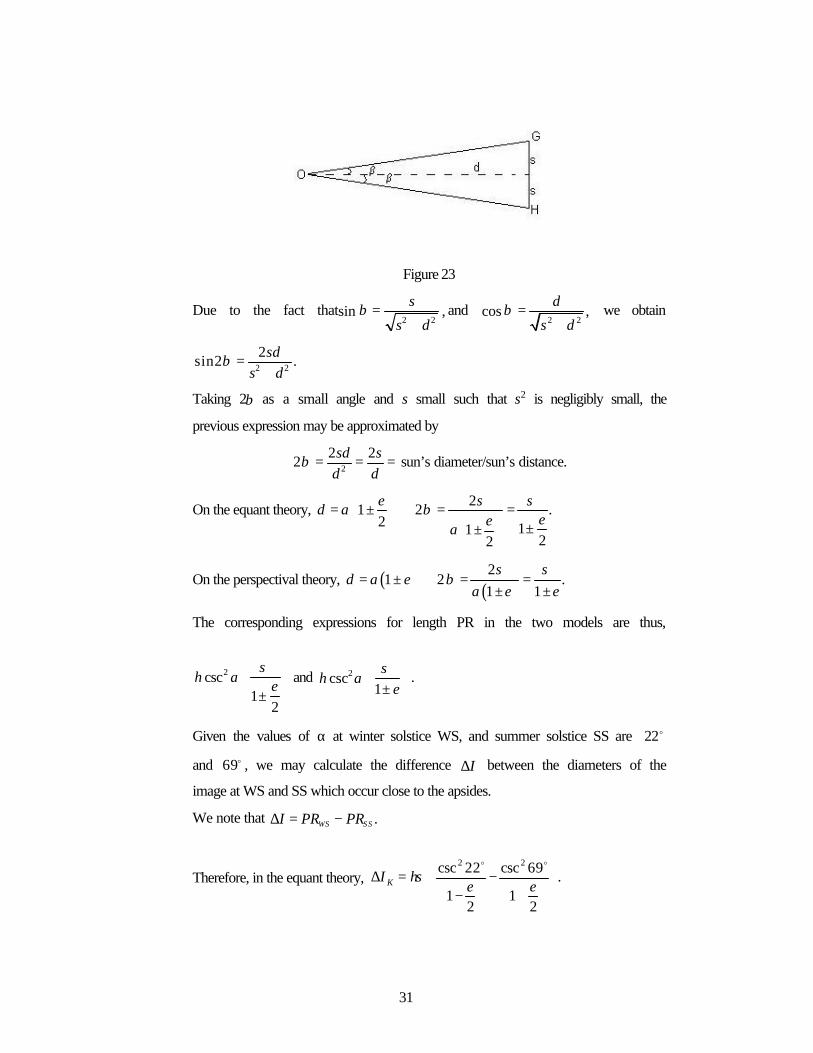
Now, see Figure 23.

31

Figure 23

Due to the fact that2 2

sin ,s

s dβ =

+and

2 2cos ,

d

s dβ =

+ we obtain

2 2

2sin2 .

sds d

β =+

Taking 2β as a small angle and s small such that s2 is negligibly small, the

previous expression may be approximated by

2

2 22

sd sd d

β = = = sun’s diameter/sun’s distance.

On the equant theory, 2

1 2 .2 11

22

e sd a

eea

σβ = ± ⇒ = = ±±

On the perspectival theory, ( ) ( )2

1 2 .1 1

sd a e

a e e

σβ= ± ⇒ = =

± ±

The corresponding expressions for length PR in the two models are thus,

2csc1

2

he

σα

±

and 2csc1

he

σα

± .

Given the values of α at winter solstice WS, and summer solstice SS are 22o

and 69o , we may calculate the difference I∆ between the diameters of the

image at WS and SS which occur close to the apsides.

We note that .WS SSI PR PR∆ = −

Therefore, in the equant theory, 2 2csc 22 csc 69

.1 1

2 2

KI he e

σ

∆ = − − +

o o

32

Or, 7 1 1 (6 4 ).2 2K

e eI h h eσ σ ∆ ≈ + − − = +

In the perspectival theory, 2 2csc 22 csc 69

1 1PI he e

σ

∆ = − − +

o o

which gives [ ]7(1 ) (1 ) (6 6 ).PI h e e h eσ σ∆ ≈ + − − = +

Take 30'σ = , 0.036,e = and 27.1h = m. This gives

(30) (27.1) 8.5(180)(60)

heπσ

= ≈

mm. In order for a decisive confirmation of

one theory over the other, Cassini had to measure σhe to within 8.5mm;

otherwise, a finding of (6 6 )I h eσ∆ = + would have decided nothing.

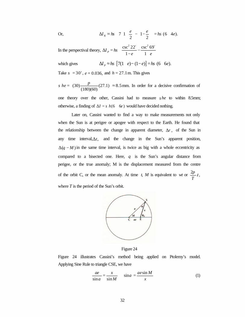
Later on, Cassini wanted to find a way to make measurements not only

when the Sun is at perigee or apogee with respect to the Earth. He found that

the relationship between the change in apparent diameter, ,ρ∆ of the Sun in

any time interval, ,t∆ and the change in the Sun’s apparent position,

( )Mθ∆ − in the same time interval, is twice as big with a whole eccentricity as

compared to a bisected one. Here, θ is the Sun’s angular distance from

perigee, or the true anomaly; M is the displacement measured from the centre

of the orbit C, or the mean anomaly. At time t, M is equivalent to wt or 2

. ,tTπ

where T is the period of the Sun’s orbit.

Figure 24

Figure 24 illustrates Cassini’s method being applied on Ptolemy’s model.

Applying Sine Rule to triangle CSE, we have

sin

sinsin sin

ae x ae MM x

αα

= ⇒ = (1)

33

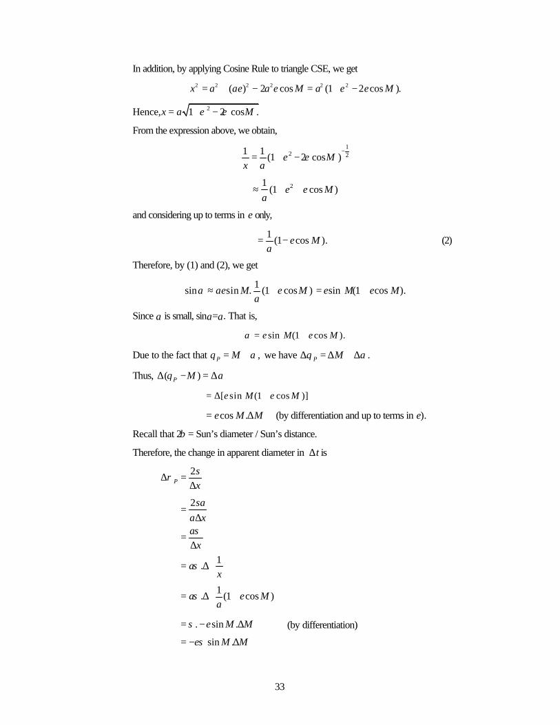
In addition, by applying Cosine Rule to triangle CSE, we get

2 2 2 2 2 2( ) 2 cos (1 2 cos ).x a ae a e M a e e M= + − = + −

Hence, 21 2 cos .x a e e M= + −

From the expression above, we obtain,

12 21 1

(1 2 cos )e e Mx a

−= + −

21(1 cos )e e M

a≈ + +

and considering up to terms in e only,

1

(1 cos ).e Ma

= − (2)

Therefore, by (1) and (2), we get

1sin sin . (1 cos ) sin (1 cos ).ae M e M e M e M

aα ≈ + = +

Since α is small, sinα=α. That is,

sin (1 cos ).e M e Mα = +

Due to the fact that ,P Mθ α= + we have .P Mθ α∆ = ∆ + ∆

Thus, ( )P Mθ α∆ − = ∆

[ sin (1 cos )]e M e M= ∆ +

cos .e M M= ∆ (by differentiation and up to terms in e).

Recall that 2β = Sun’s diameter / Sun’s distance.

Therefore, the change in apparent diameter in t∆ is

2P

sx

ρ∆ =∆

2

1.

1. (1 cos )

sa

a xa

x

ax

a e Ma

σ

σ

σ

=∆

=∆

= ∆ = ∆ +

. sin .e M Mσ= − ∆ (by differentiation)

sin .e M Mσ= − ∆

34

Hence, in interval ,t∆ the ratio of the ∆ in apparent diameter of sun to the ∆

in inequality in sun’s apparent position is

sin .

tan( ) cos .

P

P

e M MM

M e M Mρ σ σ

θ∆ − ∆= = −

∆ − ∆ (3)

Figure 25

Figure 25 illustrates Cassini’s method being applied to Kepler’s model.

Applying Sine Rule to triangle XSC, we have

11

sin2 2sin sin .

sin sin 2

ae aeMa e

MM a

ββ

= ⇒ = =

In addition, with the same rule applied to triangle ESC, we have

22

sin( )2 2sin sin sin( )

sin sin( ) 2 2

K

KK

ae aea e e

Ma

π θβ θ β

β π θ

−= ⇒ = = = +

−

where .K Mθ β= +

Consider β1 and β2 to be small angles then each of them may be approximated

by sinβ1 and sinβ2 respectively.

Since β = β1 + β2,

1 2sin sinβ β β≈ +

sin sin( )2 2

sin (sin cos cos sin )2 2

sin (1 cos ) cos sin .2 2

e eM M

e eM M M

e eM M

β

β β

β β

= + +

= + +

= + +

35

β is small and thus, by small-angle approximations,

2

sin 1 1 (cos )2 2 2

e eM M

ββ β

≈ + − +

sin cos2e

e M M β = +

1 cos sin2e

M e Mβ − =

sin

1 cos2

e Me

Mβ∴ =

−

1

sin 1 cos2

sin 1 cos .2

ee M M

ee M M

− = − = +

By applying Sine Rule to triangle XES, we have .sin sin

y aeM β

=

Hence, 1 sin

siny ae Mβ

=

sinae Mβ≈ (β is small.)

sin 1 cos2

sin1

1 cos .2

ee M M

ae Me

Ma

+ =

= +

Similar to earlier working, since ,K Mθ β= + we have .K Mθ β∆ = ∆ + ∆

Thus, ( )K Mθ β∆ − = ∆

sin 1 cos2e

e M M = ∆ +

cos .e M M= ∆ (by differentiation up to terms in e).

Therefore, the change in apparent diameter in t∆ is

2K

sy

ρ∆ =∆

36

2

1.

1. 1 cos

2

saa y

ay

ay

ea M

a

σ

σ

σ

=∆

=∆

= ∆

= ∆ +

. sin .2e

M Mσ= − ∆ (by differentiation)

sin .2e

M Mσ= − ∆

Hence in interval ,t∆ the ratio of the ∆ in apparent diameter of sun to the ∆

in inequality in sun’s apparent position is

sin .

2 tan .( ) cos . 2

K

K

eM M

MM e M M

σρ σθ

− ∆∆ = = −∆ − ∆

(4)

Comparing (3) and (4), we observe that the latter is half the result of the

former. Using the meridiana, Cassini made measurements that confirmed that

the relationship between ( )Mθ∆ − and ρ∆ was indeed that expected for the

theory of the bisected eccentricity. Thus, Kepler’s theory is confirmed as the

correct model.

37

2.4 Notes to Heilbron Pages 114 to 117 and Appendices D and E

Having discovered the model of planets traveling on elliptical orbits,

Kepler faced the problem of finding a simple geometrical method of deducing

the elements of such orbits, which include the eccentricity e and the direction

of the line of apsides ψ, from observations. Instead, he could only obtain these

values by trial and error. Once they have been found, Kepler wanted to

determine geometrically from his area law the position of planets. This is the

focus of discussion on pages 114 and 115 of Heilbron’s book which shall be

elaborated on here, with reference to W.M.Smart’s “Textbook in Spherical

Astronomy”.

Figure 26

Let the radius SZ make the angle θ with SΠ; θ is called the true

anomaly. Let a circle be described on the major axis AΠ as diameter; its radius

is thus a. Let RZ, the perpendicular from Z to AΠ, be produced to meet this

circle at Q. Then angle QCΠ is called the eccentric anomaly, denoted by η. By

properties of ellipses,

: :RZ RQ b a= (1)

where b is the semi-major axis CD.

Since sinRZ r θ= and sin sin ,RQ CQ aε η= = then by (3),

sin

sin sin .sin

r br b

a aθ

θ ηη

= ⇒ = (2)

Since cosSR r θ= and also, cos ,SR CR CS a aeη= − = − therefore

cos cos (cos ).r a ae a eθ η η= − = − (3)

38

(4)2 +(5)2 gives

2 2 2 2 2sin (cos ) .r b a eη η= + −

Using the relation 2 2 2(1 ),b a e= − and after a little reduction, we obtain

(1 cos ).r a e η= − (4)

Since 2cos 1 2sin2

r rθ

θ = − , we have 22 sin cos

2r r r

θ θ= − . Upon

substituting terms on the right hand side of the equation with (3) and (4) and

manipulation, we obtain

22 sin (1 )(1 cos ).2

r a eθ η= + − (5)

Similarly,

22 cos (1 )(1 cos ).2

r a eθ η= − + (6)

Divide (7) by (8) and taking the square root, we get

121

tan tan .2 1 2

ee

θ η+ = − (7)

Equations (4) and (7) therefore express the radius vector r and the true

anomaly θ in terms of the eccentric anomaly η. To obtain η, we turn towards

solving Kepler’s Equation.

Recall that w denotes mean angular velocity and the product ( )w t τ−

represents the angle described in an interval ( )t τ− by a radius vector rotating

about S with constant angular velocity w. We define the mean anomaly,

denoted by M, such that

( ).M w t τ= −

In Fig. 13, the area SPΠ is thus given by

Area SZΠ 1

.2

abM= (8)

To express the area in terms of the eccentric anomaly η, we consider area SZΠ

as the sum of area ZSR and area RZΠ. Take first the area of triangle PSR. Its

area is 1

.2

SRRZ .

Since cosSR CR CS a aeη= − = − and ( )sin sin ,b b

RZ RQ a ba a

η η= = =

39

area ZSR = 1

sin (cos ).2

ab eη η − Next consider area RZΠ. By application of

Cavalieri’s Principle to ellipses, we know that area RZΠ is equal to b

atimes of

area QRΠ. But area QRΠ is area of sector CQΠ minus the area of triangle

QCR, where angle QCR is η, area CQΠ is 21

2a η and area QCR is

1. cos . sin

2a aη η or 21

sin cos .2

a η η Hence,

Area RZΠ 2 21 1 1sin cos ( sin cos ).

2 2 2b

a a aba

η η η η η η = − = −

Then adding areas ZSR and RZΠ gives

Area SZΠ = 1

( sin ).2

ab η η− (9)

By equations (8) and (9), we then have

sin ( ).e M w tη η τ− = ≡ −

This is Kepler’s Equation which relates the eccentric anomaly η and the mean

anomaly M. If M and e are known, it is then possible to determine the

corresponding value of η. Thereafter, it is possible to find the value of the true

anomaly θ by substituting the values of the eccentricity e and found value of

eccentric anomaly η into equation (7); this then allows us to determine the

position of planet Z at time t.

Nonetheless, just as indicated in Heilbron’s book, even though the

Kepler’s Equation is simple to write down, it can be solved only by guesswork

and successive approximations. I shall not attempt to demonstrate how this is

done exactly but a good reference for the detailed steps is found in Smart’s

book, pages 117 – 119.

Seth Ward, professor of geometry at Oxford, had thought he found a

geometrical method that could solve Kepler’s problem simply and accurately.

40

Figure 27

With reference to Figure 27, AΠ is the line of apsides, E and S are

Earth and Sun respectively, X marks the equant point in the unoccupied focus

of the ellipse, and XS = ae. Let the mean anomaly be M whilst the true

anomaly be θ’. By extending XE to Q such that EQ = SE, and by a basic

property of ellipses, we have XQ = AΠ = 2a. In triangle XSQ, by Sine Rule,

2sin sin( ) sin[ ( )]

2sin sin( )

sin sin( ).2

ae XQ aM M

eM

eM

α π α π α

α α

α α

= =− − − +

=+

= +

Since '

,2

Mθα −= we have

' ' 'sin sin sin .

2 2 2 2 2M e M e M

Mθ θ θ− − + = + =

Then,

'sin

2 .'2 sin2

Me

M

θ

θ

− =

+

Using the above expression, the following can be deduced,

'sin

21' ' '

sin sin sin1 2 2 22' ' '

1 sin sin sin2 2 2 21

'sin

2

M

M M Me

e M M M

M

θ

θ θ θ

θ θ θ

θ

− +

+ + − ++ = =− + − − −

−+

41

'2sin cos

2 2 .'

2cos sin2 2'

tan2

tan2

M

M

M

θ

θ

θ

=

=

This equation relates the true anomaly to the apsidal distances and

mean anomaly. Hence, Ward thought he had managed to devise a geometrical

method that is simple to apply and would give the value of the true anomaly

directly. Unfortunately, Ward was wrong; his method did not give the exact

value of the true anomaly. The following gives an explanation of why this

occurred, with reference to Appendix E.

Figure 28

According to Figure 28, the true anomaly is .θ η α β= − +

In triangle CPR,

ˆsin sin .ˆsin sin

RP a RPCPR

aCPRα

α= ⇒ = (1)

By Cavalieri’s Principle, .b

PQ RQa

=

However in triangle CRQ, sin sin .RQ

RQ aa

η η= ⇒ =

Then RP RQ PQ= − sin sina bη η= −

( )sina b η= − (2)

Since ˆ 90 ,CRQ η= −o ˆ ˆ180CPR CRQα= − −o

180 (90 )α η= − − −o o

42

90 ( )α η= − −o (3)

Substitute (2) and (3) in (1), we get

sin sin sin[90 ( )]a b

aα η α η−= − −o

sin cos( )

1 sin cos( )

a ba

ba

η α η

η η α

−= −

= − −

1 sin cos ,ba

η η = −

where α is small.

By properties of ellipses, 2

2 2 12e

b a = −

2 2

2 14

b ea

= −

12 22

1 14 8

b e ea

= − ≈ −

Hence, 2

sin sin cos .8eα η η≈ In addition, α is small. Thus,

2

sin cos .8eα η η≈

Similarly, in triangle CPF, by Sine Rule,

sin2 2sin sin( ) .

sin sin( ) 2 1 cos2

ae ePF ae

ePF

ηβ η α

β η α η= ⇒ = − =

− −

β is small and thus by approximation, sin

2 .1 cos

2

e

e

ηβ

η=

−

Recall that .θ η α β= − +

Hence, 2 sin

2sin sin cos2 8 1 cos

2

ee e

Me

ηθ η η η

η= + − +

−

2

sin sin cos sin 1 cos2 8 2 2e e e e

M η η η η η ≈ + − + +

43

To express sinη in terms of e and M, we have

sin sin sin2e

Mη η = +

2

sin sin sin2 2

sin sin cos sin cos sin2 2 2

sin sin 1 sin cos . sin2 4 2

e eM M

e e eM M M

e e eM M M

η

η η

η η

= + + = + +

≈ + − +

sin sin2e

M M = + (up to first order terms in e)

2

2

sin cos sin cos sin sin2 2

sin 1 sin cos . sin4 2

sin sin cos .2

e eM M M M

e eM M M M

eM M M

= +

≈ − +

= +

To express cosη in terms of e and M, we have

cos cos sin2e

Mη η = +

cos sin sin cos2 2

cos cos sin sin cos sin sin sin sin cos2 2 2 2

e eM M M M

e e e eM M M M M M M M

= + + = + − +

cos sin . sin2

eM M M≈ − (up to first order terms in e)

2cos sin .2e

M M= −

Thus,

22sin sin cos sin sin cos cos sin

2 2 8 2 2e e e e e

M M M M M M M M Mθ = + + − + −

44

2

2 2 2

2

sin sin cos 1 cos sin2 2 2 2

sin sin2 sin2 sin sin22 8 16 2 4

5sin sin2 .

16

e e e eM M M M M

e e e e eM M M M M M

M e M e M

= + + −

= + + − + +

= + +

Referring to Figure 27, in triangle XSQ, by Sine Rule,

sin sin(180 )

2sin sin(180 ( ))

2sin sin( )

sin sin( )2

sin sin cos cos sin2 2

tan sin cos tan .2 2

ae XQM

ae aM

eM

eM

e eM M

e eM M

α α

α α

α α

α α

α α α

α α

=− −

=− +

=+

= +

= +

= +

o

o

tan 1 cos sin2 2e e

M Mα − =

sin

2tan .1 cos

2

eM

eM

α∴ =−

Consider α a small angle. Then by small angle approximations, tan .α α≈

Since ' 2 ,Mθ α= + we have

sin'

1 cos2

e MM

eM

θ ≈ +−

2

sin 1 cos2

sin sin24

eM e M M

eM e M M

≈ + +

= + +

45

Thus, 21' sin2 .

16e Mθ θ− = In other words, there was a discrepancy of a

maximum 21sin2

16e M between Ward’s found value for “true anomaly” and

the actual true anomaly.

46

References:

1. Evans, J., Am. J. Phys. 52 (12), 1080 (1984)

2. Evans, J., Am. J. Phys. 56 (11), 1009 (1988)

3. Hahn, Alexander J. Basic Calculus: from Archimedes to Newton to its role in

science. New York: Springer-Verlag, 1998.

4. Heilbron, J.L. The Sun in the Church: Cathedrals as Solar Observatories

Cambridge: Harvard University Press, 1999.

5. Hoskin, Michael. The Cambridge Illustrated of Astronomy . Cambridge:

Cambridge University Press, 1997.

6. Neugebauer, O. The Exact Sciences in Antiquity. Princeton: Princeton

University Press, 1952.

7. Smart, W.M. Textbook on Spherical Astronomy, Fourth Edition. Cambridge:

Cambridge University Press, 1960.

8. O’Connor, J.J. and Robertson, E.F., The MacTutor History of Mathematics

Archive, http://www-groups.dcs.st-andrews.ac.uk/~history/Mathematicians/,

University of St Andrews Scotland, Mar 2001.