a maximum entropy model of phonotactics and -...
TRANSCRIPT

A Maximum Entropy Model of Phonotactics and Phonotactic Learning
Bruce Hayes Colin Wilson [email protected] [email protected]
Preprint version, August 2007
Abstract
The study of phonotactics (e.g., the ability of English speakers to distinguish possible words like blick from impossible words like *bnick) is a central topic in phonology. We propose a theory of phonotactic grammars and a learning algorithm that constructs such grammars from positive evidence.
Our grammars consist of constraints that are assigned numerical weights according to the principle of maximum entropy. Possible words are assessed by these grammars based on the weighted sum of their constraint violations. The learning algorithm yields grammars that can capture both categorical and gradient phonotactic patterns. The algorithm is not provided with any constraints in advance, but uses its own resources to form constraints and weight them. A baseline model, in which Universal Grammar is reduced to a feature set and an SPE-style constraint format, suffices to learn many phonotactic phenomena. In order to learn nonlocal phenomena such as stress and vowel harmony, it is necessary to augment the model with autosegmental tiers and metrical grids. Our results thus offer novel, learning-theoretic support for such representations.
We apply the model to English syllable onsets, Shona vowel harmony, quantity-insensitive stress typology, and the full phonotactics of Wargamay, showing that the learned grammars capture the distributional generalizations of these languages and accurately predict the findings of a phonotactic experiment.
Keywords: phonotactics, maximum entropy, learnability, onsets, Shona, Wargamay
Hayes/Wilson Maximum Entropy Phonotactics p. 2
1. Introduction*
In one of the central articles from the early history of generative phonology, Chomsky and Halle (1965) lay out a research program for the theory of phonotactics. They begin with the observation that the logically possible sequences of English phonemes can be divided into three categories:
(1) a. Existing words, such as brick b. Nonexisting words that are judged by native speakers to be well-formed, such as
blick. c. Nonexisting words that are judged by native speakers to be ill-formed, such as
bnick.
The scientific challenge posed by this categorization has two parts. The first is to characterize the grammatical knowledge that permits native speakers to make phonotactic well-formedness judgments. The second, more fundamental challenge is to understand the principles with which phonotactic grammars are acquired.
The difficulty of this task is evident from a further point made by Chomsky and Halle, namely that there are grammars that fully account for the learning data but fail to capture the native speaker’s knowledge. For example, they note that both of the rules given in (2) are compatible with the data available to the learner. However, while the rule in (2a) correctly excludes *bnick, it also excludes the acceptable form blick. In contrast, (2b) appropriately excludes *bnick but allows blick as a possible word.
(2) a. Consonantal Segment → r / # b___k b. Consonantal Segment → Liquid / # Stop ___ Vowel
The problem of phonotactic learning, then, is that of selecting a particular grammar — the one that is in fact acquired by native speakers — from among all of the possible grammars that are compatible with the learning data. Chomsky and Halle schematize the selection process as follows, where “AM” is the universal mechanism, or acquisition model, that projects grammars from data.
(3) primary linguistic data → AM → grammar
In this article, we take up the challenge posed by Chomsky and Halle, proposing an explicit theory of phonotactic grammars and of how those grammars are learned. We propose that phonotactic grammars are composed of numerically-weighted constraints, and that the well-formedness of an output is formalized as a probability determined by the weighted sum of its
* We would like to thank two anonymous LI reviewers, Steven Abney, Paul Boersma, Michael Hammond, Robert Kirchner, Robert Malouf, Joe Pater, Donca Steriade, Kie Zuraw, and audiences at the University of Michigan, the University of California at San Diego, the University of Arizona, and UCLA for helpful input on our project. Special thanks to Jason Eisner for alerting us to the feasibility of using finite state machines to formalize the computations of our model.
Hayes/Wilson Maximum Entropy Phonotactics p. 3
constraint violations. We further propose a learning model in which constraints are selected from a constraint space provided by UG and assigned weights according to the principle of maximum entropy. This model learns phonotactic grammars from representative sets of surface forms. We apply the model to data from a number of languages, showing that the learned grammars capture the distributional generalizations of the languages and accurately predict experimental findings.
The organization of the paper is as follows. §2 elaborates our research goals in constructing a phonotactic learner, while §3 and §4 describe our learning model in detail. The next four sections are case studies, covering English syllable onsets (§5), Shona vowel harmony (§6), stress systems (§7), and finally a whole-language analysis, Wargamay (§8). In the concluding section (§9), we address questions raised by our work and outline directions for future research.
2. Goals of a phonotactic learner
We claim that the following criteria are appropriate for evaluating theories of phonotactics and phonotactic learning.
2.1 Expressiveness
The findings of the last few decades demonstrate a striking richness of structures and phenomena in phonology, including long-distance dependencies (e.g., McCarthy 1988), phrasal hierarchies (e.g. Selkirk 1980a), metrical hierarchies (e.g. Liberman and Prince 1977), elaborate interactions with morphology (e.g. Kiparsky 1982), and other areas, each the subject of extensive analysis and research. We anticipate that a successful model of phonotactics and phonotactic learning will incorporate theoretical work from all of these areas.
A particular consequence of this richness is that the principles governing phonotactics are cross-classifying: the legality of (say) a particular vowel may depend simultaneously on the various natural classes to which it belongs, its immediate segmental neighbors, its neighbors on a vowel tier (§6), and the position of its syllable in a metrical stress hierarchy. Previous accounts of phonotactic learning, however, have relied on just a single classification of environments. For instance, traditional n-gram models (Jelinek 1999, Jurafsky and Martin 2000) are quite efficient and have broad application in industry, but they define only an immediate segmental context and are thus insufficient as a basis for phonotactic analysis (§5.3, §6). Similarly, the stochastic context-free grammar of Coleman and Pierrehumbert (1997), while more phonologically sophisticated, rests on a single partition of words into onsets and rimes. As Coleman and Pierrehumbert point out, this makes it impossible in principle for the model to capture the many phonotactic restrictions that cross onset-rime boundaries (Clements and Keyser 1983:20-21) or syllable boundaries (bans on geminates, heterorganic nasal-stop clusters, sibilant clusters).
The maximum entropy approach to phonotactics, like many others, is based on phonological constraints. 1 Crucially, however, it makes no commitments about the content of these
1 The use of constraints is the most widely adopted general approach to phonotactics. The alternative strategy of “licenses” is also the subject of current research: see Albright (2006) and Heinz (to appear a, to appear b).

Hayes/Wilson Maximum Entropy Phonotactics p. 4
constraints, leaving this as a question of phonological theory. Moreover, as we will show, maximum entropy models can assess well-formedness using cross-classifying principles.
2.2 Providing an inductive baseline
While we have emphasized the primacy of phonological theory, the precise content of the latter remains an area of considerable disagreement. A computational learning model can be used as a tool for evaluating and testing theoretical proposals. The idea is that a very simple theory can provide a sort of inductive baseline against which more advanced theories can be compared. If the introduction of a theoretical concept makes possible the learning of phonotactic patterns that are inaccessible to the baseline system, the concept is thereby supported. For earlier work pursuing the inductive baseline approach, see Gildea and Jurafsky 1996, Peperkamp et al. 2006.
Our own inductive baseline is a purely linear, feature-bundle approach modeled on Chomsky and Halle (1968; henceforth SPE). To this we will add the concepts of autosegmental tier (Goldsmith 1979) and metrical grid (Liberman 1975, Prince 1983), showing that both make possible modes of phonotactic learning that are unreachable by the linear baseline model.
2.3 Accounting for gradience
All areas of generative grammar that address well-formedness are faced with the problem of accounting for gradient intuitions. A large body of research in generative linguistics deals with this issue; for example Chomsky 1963, Ross 1972, Legendre et al. 1990, Schütze 1996, Hayes 2000, Boersma and Hayes 2001, Boersma 2004, Keller 2000, 2006, Sorace and Keller 2005, and Legendre et al. 2006. In the particular domain of phonotactics, gradient intuitions are pervasive: they have been found in every experiment that allowed participants to rate forms on a scale (e.g., Greenberg and Jenkins 1964, Ohala and Ohala 1986, Coleman and Pierrehumbert 1997, Vitevitch et al. 1997, Frisch et al. 2000, Treiman et al. 2000, Bailey and Hahn 2001, Hay, Pierrehumbert, and Beckman 2003, Coetzee 2004, Hammond 2004, Berent et al., 2007). Gradience is also found in the frequency of “repairs” (such as excrescent vowel insertion) participants make when asked to utter illegal nonce forms (Davidson 2006). Gradient intuitions can be found even among forms that satisfy the categorical phonotactics of the language, but contain rare sequences (Frisch et al. 2000, Bailey and Hahn 2001). Thus, we consider the ability to model gradient intuitions to be an important criterion for evaluating phonotactic models. As we will show below, it is an inherent property of maximum entropy models that they can account for both categorical and gradient phonotactics in a natural way.
To sum up, we seek to solve Chomsky and Halle’s problem, specifying the structure of the module AM and testing it on actual phonotactic systems, with the goal of describing the full range of data including gradient intuitions. As a research strategy, we adopt the inductive baseline approach, requiring that phonological theories justify themselves through improvements in learning performance. To this end, we adopt an overall framework for learning, maximum entropy, that is neutral with regard to the constraints employed. We turn next to the structure of this model.
Hayes/Wilson Maximum Entropy Phonotactics p. 5
3. Maximum entropy grammars
A maximum entropy grammar uses weighted constraints to assign probabilities to outputs. For general background on maximum entropy (hereafter, maxent) grammars, see Jaynes 1983, Jelinek 1999:ch. 13, Manning and Schutze 1999, and Klein and Manning 2003. We will rely here on particular results developed in Berger et al. 1996, Rosenfeld 1996, Della Pietra et al. 1997, and Eisner 2001. For earlier applications of maxent grammars to phonology, in particular to the learning and analysis of input-output mappings, see Goldwater and Johnson 2003 and Jäger 2004.
Maxent grammars have special properties that recommend them as a basis for phonotactic learning. They have been subject to thorough mathematical analysis that establishes their convergence properties and their connection to the theories of information and statistical estimation. In addition, the solutions they embody can be said to have a highly principled character, discussed in the remainder of this section.
3.1 The probabilistic conception of phonotactic well-formedness
The core idea in the application of maxent grammars to phonotactics is that well-formedness can be interpreted as probability. We suppose an infinite set Ω consisting of all universally-possible phonological surface forms. To every member x of this set, a maxent grammar assigns a probability P(x) which expresses its phonotactic well-formedness. Naturally, the probability of any one given form will be extremely small. What is important is the differences between these probabilities, which (as we will show) can be large and meaningful.
Our working hypothesis is that, provided the constraint set is an adequate one, the probabilities assigned to forms by a maxent grammar will correspond with the well-formedness judgments of native speakers, with lower probabilities for forms judged less acceptable.
3.2 Assigning probability in maxent grammars
A maxent grammar assigns probabilities with a set of constraints, stated in the chosen representational vocabulary. The constraints are free to refer to all of the featural, structural, and other distinctions made by the representations, and thus permit multiple overlapping characterizations of phonological forms, argued above (§2.1) to be crucial to an adequate phonotactic model.
All of the constraints in our model are Markedness constraints, in the sense of Optimality Theory (“OT”; Prince and Smolensky 1993/2004). No role is played by inputs or by OT-style Faithfulness constraints. This decision is sensible in light of the task at hand: we seek to assess forms simply for their phonological legality, not for their legality as derived from some particular input. Some consequences of this decision are assessed in §9 below.
Every constraint in the grammar has a weight, a nonnegative real number. The weights can be thought of as scaling the importance of one constraint relative to others. Constraints with higher weights have a more powerful effect in lowering the probability of forms that violate them.
Hayes/Wilson Maximum Entropy Phonotactics p. 6
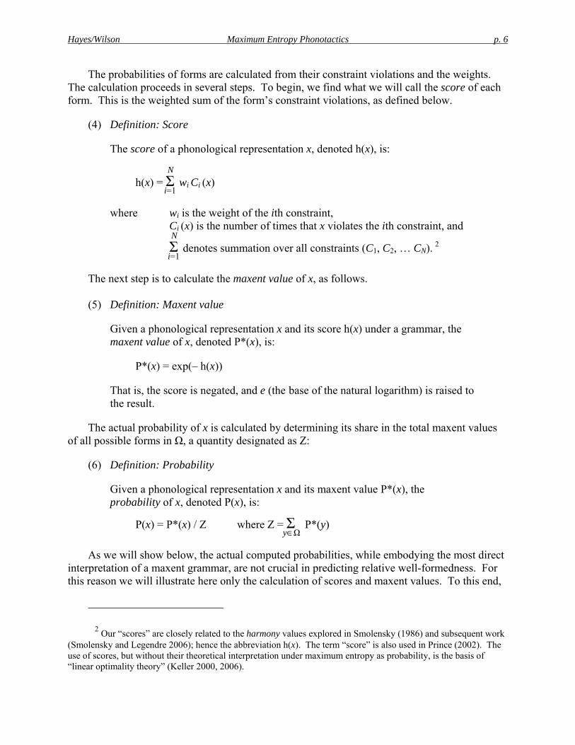
The probabilities of forms are calculated from their constraint violations and the weights. The calculation proceeds in several steps. To begin, we find what we will call the score of each form. This is the weighted sum of the form’s constraint violations, as defined below.
(4) Definition: Score
The score of a phonological representation x, denoted h(x), is:
h(x) = Σi=1
N wi Ci (x)
where wi is the weight of the ith constraint, Ci (x) is the number of times that x violates the ith constraint, and
Σi=1
N denotes summation over all constraints (C1, C2, … CN). 2
The next step is to calculate the maxent value of x, as follows.
(5) Definition: Maxent value
Given a phonological representation x and its score h(x) under a grammar, the maxent value of x, denoted P*(x), is:
P*(x) = exp(– h(x))
That is, the score is negated, and e (the base of the natural logarithm) is raised to the result.
The actual probability of x is calculated by determining its share in the total maxent values of all possible forms in Ω, a quantity designated as Z:
(6) Definition: Probability
Given a phonological representation x and its maxent value P*(x), the probability of x, denoted P(x), is:
P(x) = P*(x) / Z where Z = Σy∈Ω
P*(y)
As we will show below, the actual computed probabilities, while embodying the most direct interpretation of a maxent grammar, are not crucial in predicting relative well-formedness. For this reason we will illustrate here only the calculation of scores and maxent values. To this end,
2 Our “scores” are closely related to the harmony values explored in Smolensky (1986) and subsequent work (Smolensky and Legendre 2006); hence the abbreviation h(x). The term “score” is also used in Prince (2002). The use of scores, but without their theoretical interpretation under maximum entropy as probability, is the basis of “linear optimality theory” (Keller 2000, 2006).
Hayes/Wilson Maximum Entropy Phonotactics p. 7
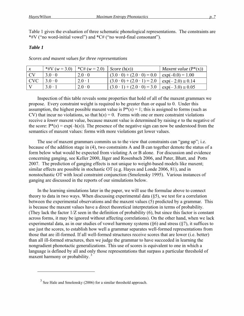
Table 1 gives the evaluation of three schematic phonological representations. The constraints are *#V (“no word-initial vowel”) and *C# (“no word-final consonant”).
Table 1
Scores and maxent values for three representations
x *#V (w = 3.0) *C# (w = 2.0) Score (h(x)) Maxent value (P*(x)) CV 3.0 · 0 2.0 · 0 (3.0 · 0) + (2.0 · 0) = 0.0 exp(–0.0) = 1.00 CVC 3.0 · 0 2.0 · 1 (3.0 · 0) + (2.0 · 1) = 2.0 exp(– 2.0) ≅ 0.14 V 3.0 · 1 2.0 · 0 (3.0 · 1) + (2.0 · 0) = 3.0 exp(– 3.0) ≅ 0.05
Inspection of this table reveals some properties that hold of all of the maxent grammars we
propose. Every constraint weight is required to be greater than or equal to 0. Under this assumption, the highest possible maxent value is P*(x) = 1; this is assigned to forms (such as CV) that incur no violations, so that h(x) = 0. Forms with one or more constraint violations receive a lower maxent value, because maxent value is determined by raising e to the negative of the score: P*(x) = exp(–h(x)). The presence of the negative sign can now be understood from the semantics of maxent values: forms with more violations get lower values.
The use of maxent grammars commits us to the view that constraints can “gang up”; i.e. because of the addition stage in (4), two constraints A and B can together demote the status of a form below what would be expected from violating A or B alone. For discussion and evidence concerning ganging, see Keller 2000, Jäger and Rosenbach 2006, and Pater, Bhatt, and Potts 2007. The prediction of ganging effects is not unique to weight-based models like maxent; similar effects are possible in stochastic OT (e.g. Hayes and Londe 2006, 81), and in nonstochastic OT with local constraint conjunction (Smolensky 1995). Various instances of ganging are discussed in the reports of our simulations below.
In the learning simulations later in the paper, we will use the formulae above to connect theory to data in two ways. When discussing experimental data (§5), we test for a correlation between the experimental observations and the maxent values (5) predicted by a grammar. This is because the maxent values have a direct theoretical interpretation in terms of probability. (They lack the factor 1/Z seen in the definition of probability (6), but since this factor is constant across forms, it may be ignored without affecting correlations). On the other hand, when we lack experimental data, as in our studies of vowel harmony systems (§6) and stress (§7), it suffices to use just the scores, to establish how well a grammar separates well-formed representations from those that are ill-formed. If all well-formed structures receive scores that are lower (i.e. better) than all ill-formed structures, then we judge the grammar to have succeeded in learning the nongradient phonotactic generalizations. This use of scores is equivalent to one in which a language is defined by all and only those representations that surpass a particular threshold of maxent harmony or probability.
3
3 See Hale and Smolensky (2006) for a similar threshold approach.
Hayes/Wilson Maximum Entropy Phonotactics p. 8
3.3 Learning maxent weights
Up to this point, we have defined maxent grammars and described how well-formedness is calculated from constraint violations and weights. We turn now to the question of learning. Our starting assumption (see, e.g., Baker 1979) is that the learner has access to a large and representative set of observed forms drawn from the target language. However, it has no access to “negative evidence”; that is, it is never told what forms are illegal. This plausibly corresponds to the situation faced by real language learners.
Postponing to §4 the question of how to find the constraints, we consider here first the problem of finding the weights for a known set of constraints.
3.3.1 Defining the objective
The objective here is to find the set of constraint weights that maximizes the probability of the observed forms. Because total probability is fixed (at 1), maximizing the probability of the observed forms will minimize the probability of the unobserved forms—or more precisely, the unobserved forms that differ in a principled way from the observed forms, as determined by the constraint set. Given our probabilistic conception of well-formedness (§3.1), this objective for constraint weighting embodies the traditional goals of phonotactic analysis.
The term “maximum entropy” relates to this goal. “Entropy” is an information-theoretic measure of the amount of randomness in the system, given by the formula – Σ
x∈Ω P(x) log(P(x))
(Cover and Thomas 1991). According to a theorem proved by Della Pietra et al. (1997), if probability is defined as in §3.2, maximizing entropy is in fact equivalent to maximizing the probability of the observed forms given the constraints.
Under the standard assumption that the forms in the observed data are independent and identically distributed, the probability of the observed data P(D) is simply the product of the probabilities of all the individual data.
(7) Probability of the observed data under a given set of constraints and weights
Given a maxent grammar and a set D of observed data, the probability of D under the grammar is:
P(D) = Πx∈D P(x)
where P(x) is as defined in (6).

Hayes/Wilson Maximum Entropy Phonotactics p. 9
Finding the set of weights that maximizes P(D) is a search problem, to whose solution we now turn.4
3.3.2 Finding the weights
The search begins by giving every constraint the same initial weight; in our simulations, this value is always 1. The system then carries out an iterated calculation intended to maximize P(D). The calculation follows an ascending path on the multidimensional surface defined by the weights, achieving ever higher values for P(D) until the highest possible value has been reached.
For mathematical convenience, the search actually finds the maximum for the natural logarithm of P(D), not P(D) itself. Since the log function is monotonic, the weights that maximize log(P(D)) are the same are the weights that maximize P(D).
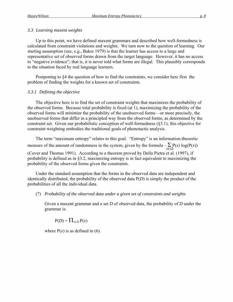
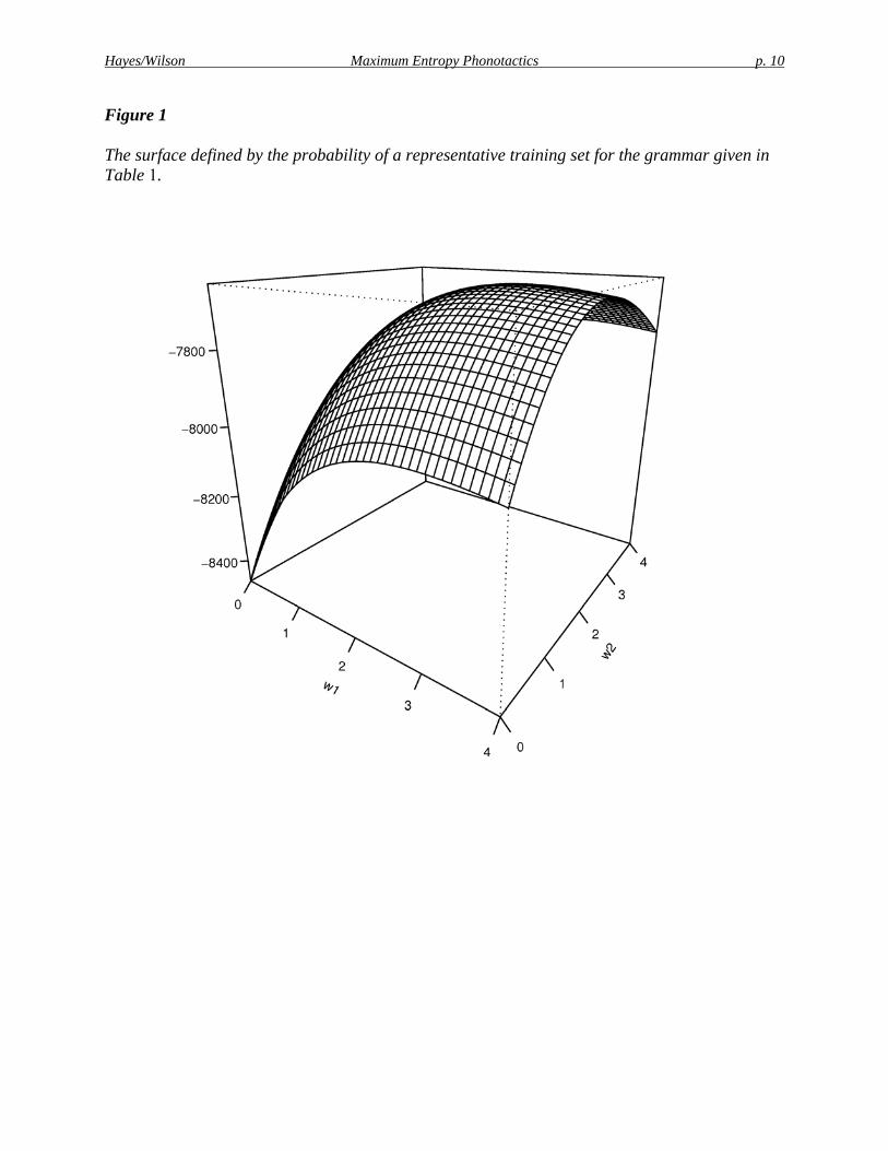
The process of iterative ascent is illustrated in the two figures below, which depict the learning of the constraint weights for the two-constraint grammar discussed in Table 1. Figure 1 shows the three-dimensional surface corresponding to the search space, with the horizontal dimensions corresponding to the two constraint weights and the vertical dimension to log(P(D)).5 Figure 2 gives the same information in the form of a contour map and includes the actual path taken during learning. The ascent terminates at the peak (3, 2), where the log probability of the training data is maximized at log(P(D)) = –7641.8.
4 The text of this section oversimplifies, as it is standard in maximum entropy modeling to prevent overfitting (Duda, Hart, and Stork 2001, 5) by adding a term to the objective in (8) that penalizes large weights. We used the Gaussian prior, discussed in Goldwater and Johnson 2003:§2, setting the parameters μ and σ to 0 and 1, respectively.
5 The latter was approximated by assuming that all strings (composed of C and V) were of length 10 or less.
Hayes/Wilson Maximum Entropy Phonotactics p. 10
Figure 1
The surface defined by the probability of a representative training set for the grammar given in Table 1.
Hayes/Wilson Maximum Entropy Phonotactics p. 11
Figure 2
Iterative ascent of the surface given in Figure 1
The strategy pursued here never actually calculates the surface as a whole, but instead
determines at each stage the local gradient, or slope. This indicates the direction (uphill) that the next search iteration should take. This procedure is guaranteed to converge on the weights that maximize log(P(D)) because, as Della Pietra et al. (1997) show, in a maxent grammar the surface being ascended is always convex; that is, it contains no local maxima in which the search could get stuck. Following the gradient also suffices to indicate when the upward journey can be terminated: this is when the slope becomes sufficiently close (by an arbitrarily-chosen small value) to zero. There are many algorithms that can iteratively ascend a surface given the gradient. We used the Conjugate Gradient method (Press et al. 1992), which is known to converge quickly for this type of problem (Malouf 2002).
The heart of the calculation is the determination of the gradients. Formally, the gradient consists of a vector of partial derivatives, one for each constraint in the grammar. Each partial
Hayes/Wilson Maximum Entropy Phonotactics p. 12
derivative has the form ∂wi∂ log(P(D)) and expresses the rate at which log(P(D)) responds to local
changes in the weight assigned to constraint Ci. The computation of the partial derivatives will depend on the current location along the surface and on the constraint violations in the learning data.
As Della Pietra et al. (1997) showed (see also Berger, n.d.), each partial derivative ∂wi∂ log(P(D)) is equal to an intuitively interpretable value, namely the difference between the
number of observed violations of Ci and the number of expected violations, a value denoted O[Ci] – E[Ci]. Thus, if we can determine both the observed and the expected violations for all constraints, we will know the direction in which the iterative search should continue, and converge on the right answer.
Calculating the observed violation count of a constraint O[Ci] is straightforward: one simply sums the violations of the constraint over all examples in the learning data. However, calculating the expected violation count E[Ci] is more difficult—seemingly impossible, in fact—since we must sum over the set of all possible phonological representations x ∈ Ω, an infinite set. Postponing this issue momentarily, we first define expected violation count formally, as a probability-weighted sum:
(8) Definition: Expected number of violations
Given a grammar that determines maxent values, the expected number of violations of constraint Ci is:
E[Ci] = Σx∈Ω P(x) Ci(x)
where
P(x) is the probability of the representation x, Ci(x) is the number of times that x violates Ci, and Σx∈Ω represents summation of over all x in Ω.
Instead of calculating expected values exactly, we approximate them by examining only the strings in Ω that are no longer than the longest string in the learning data D. This is a finite—albeit exponentially large—subset of Ω, and to sum over it we employ methods borrowed from work in computational OT (Ellison 1994, Eisner 1997, Albro 1998, 2005, Riggle 2004). As this work has shown, the properties of a very large set of strings can be computed by representing the set as a finite state machine. We construct our machines by first representing each constraint as a weighted finite-state acceptor. Using intersection (Hopcroft and Ullman 1979), the constraints are then combined into a single machine that embodies the full grammar (Ellison 1994, Riggle 2004). Each path through this machine corresponds to a phonological representation together with its vector of constraint violations. We then obtain the E[Ci] values by summing over all paths through the machine, using a method devised by Eisner (2001, 2002). The sum over all
Hayes/Wilson Maximum Entropy Phonotactics p. 13
paths of a given length is rescaled according to the frequency of forms of that length in the learning data.
We now summarize the procedure for constraint weighting. The core process is an iterated hill-climbing search, designed to maximize the probability of the learning data (P(D)). The search is determined at each stage by calculating a local gradient based on the observed/expected difference O[Ci] – E[Ci] for each constraint. O[Ci] is determined by inspection of the learning data, while E[Ci] is calculated by the finite-state method described immediately above.
4. Searching the space of possible constraints
In principle, there exists a maxent grammar that succeeds fully in the goal of maximizing the probability of the learning data: it would deploy constraints with such an extreme degree of detail that they banned all and only the nonobserved data. Such a grammar is of no interest, because it wrongly excludes nonexistent but possible forms like blick (§1). Grammar learning becomes interesting—becomes a phonological problem—when we attempt to learn more general constraints that have the capacity to predict which novel forms will be phonologically legal. However, even when the problem is considered in this way, one still faces a formidable difficulty: the fact that an enormous number of distributional generalizations are consistent with any given set of surface forms. We must therefore find a strategy for navigating the space of possible generalizations and selecting members of that space for inclusion in the grammar.
Previous research on phonotactic learning has not addressed the selection problem in a general form. Work in Optimality Theory (Hayes 2004, Prince and Tesar 2004, Jarosz 2006, Pater and Coetzee 2006) generally assumes that the constraint set is provided by UG. No selection problem arises under this approach, as learning consists simply of assigning a ranking to the constraint set. The parameter setting approach set forth in Dresher and Kaye 1990 likewise confronts no selection problem, since the parameters and their cues are provided a priori. However, our interest in establishing an inductive baseline (§2.2) is incompatible with any rich UG approach, either constraint-based or parametric. Though it may be necessary to add specific universal constraints to UG, our present goal is to determine how much of phonotactic learning can be done without them.
Another option not open to us is simply to incorporate every possible constraint into the grammar, relying on the weighting algorithm to determine the importance of each one. This is essentially the proposal of Pierrehumbert (2006), who applies it to the analysis of medial consonant clusters. This strategy might be successful when the number of constraints is limited to a small set, either because the empirical domain is restricted or because the theory of UG assumed tightly limits the number of possible constraints. However, neither condition is met here.
To solve the selection problem, we assume that UG determines the feature inventory and the format of constraints, yielding a search space that is quite large, and hence compatible with the inductive baseline approach. Nevertheless, in our experience it is effectively searchable, provided the right search heuristics are used. In what follows, we first give our proposals for limiting the constraint space, then cover the search heuristics.

Hayes/Wilson Maximum Entropy Phonotactics p. 14
Like other properties of our learner, our proposals concerning the search space and heuristics constitute a theoretical claim about language learning. To be sure, they are also motivated by issues of implementation—but not, we think, in a way that sacrifices realism with respect to the human learner. If we have characterized the problem of learning phonotactic correctly, then the human learner faces the same search problem as our mechanical learner. The claim is that humans perform the search for phonotactics in a way that is functionally identical to the strategy we describe.
4.1 The constraint space
The learner is assumed to be provided with a set of features, the inventory of segments in the target language, and the feature specifications for each of those segments.6 For our purposes, it is the natural classes determined by the features, rather than the features themselves, that determine the content of a constraint. Many natural classes have multiple featural definitions, and it is immaterial which particular definition is used to state a constraint. To locate the natural classes determined by a segment inventory and feature set, we use an algorithm and software created by Kie Zuraw.
4.1.1 Constraint format
Using the natural classes, we construct two basic constraint types. The first type is just a sequence of feature matrices, as in (9).
(9)*
Here, F, G … are features and α, β, … take the values + and –. Such a constraint is matched to representations as in SPE. It acts as a function, returning the number of matches.
. . .
αFβ G
γH
. . . δI
εJ
. . .
… ζK
We also assume (cf. Halle 1959, Stanley 1967, SPE ch. 7, Fudge 1969, Prince and Smolensky 1993/2004) that constraints may include logical implication; schematically, “if a particular segment has feature values [αF, βG, … ], then any preceding/following segment must have the values [γH, δI … ].” An example from the grammar of English onsets is the following: “if a nasal occurs in an onset, any preceding sound must be [s]” (Fudge 1969:279, Selkirk 1982:346). This is straightforward to state as an implication. But without the capacity for implication, we would instead have to formulate a set of constraints that jointly ban every segment except [s] in the context / # ___ [+nas]. Many similar cases can be found.
To formalize implication, we allow exactly one of the matrices of a constraint to be modified by the complementation operator ^; thus [^αF, βG, … ] means any segment not a
6 For work on the learning of segments and features from the input signal, see Boersma, Escudero and Hayes 2003, Mielke 2004, Lin 2005b, and Goldsmith and Xanthos 2006.
Hayes/Wilson Maximum Entropy Phonotactics p. 15
member of the natural class [αF, βG, … ]. For example, the constraint proposed by Fudge and Selkirk limiting prenasal segments to [s] would be formulated as *[^–voice,+ant,+strid][+nasal]. A slightly more general version of this is actually learned by our system; see Table 4, #3 below.7
As we will see (§5.3.2), the use of implicational constraints produces an improvement (albeit a modest one) in the performance of our system. It also creates grammars that are smaller and easier to interpret.
4.1.2 Limiting the number of possible constraints
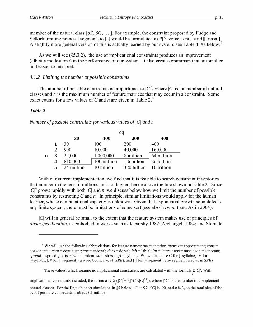
The number of possible constraints is proportional to |C|n, where |C| is the number of natural classes and n is the maximum number of feature matrices that may occur in a constraint. Some exact counts for a few values of C and n are given in Table 2.8
Table 2
Number of possible constraints for various values of |C| and n
|C| 30 100 200 400 1 30 100 200 400 2 900 10,000 40,000 160,000 n 3 27,000 1,000,000 8 million 64 million 4 810,000 100 million 1.6 billion 26 billion 5 24 million 10 billion 320 billion 10 trillion
With our current implementation, we find that it is feasible to search constraint inventories that number in the tens of millions, but not higher; hence above the line shown in Table 2. Since |C|n grows rapidly with both |C| and n, we discuss below how we limit the number of possible constraints by restricting C and n. In principle, similar limitations would apply for the human learner, whose computational capacity is unknown. Given that exponential growth soon defeats any finite system, there must be limitations of some sort (see also Newport and Aslin 2004).
|C| will in general be small to the extent that the feature system makes use of principles of underspecification, as embodied in works such as Kiparsky 1982; Archangeli 1984; and Steriade
7 We will use the following abbreviations for feature names: ant = anterior; approx = approximant; cons = consonantal; cont = continuant; cor = coronal; dors = dorsal; lab = labial; lat = lateral; nas = nasal; son = sonorant; spread = spread glottis; strid = strident; str = stress; syl = syllabic. We will also use C for [–syllabic], V for [+syllabic], # for [–segment] (a word boundary; cf. SPE), and [ ] for [+segment] (any segment, also as in SPE).
8 These values, which assume no implicational constraints, are calculated with the formula Σi=1
n |C|i. With
implicational constraints included, the formula is Σi=1
n (|C|i + i(|^C|×|C|i-1)), where |^C| is the number of complement
natural classes. For the English onset simulation in §5 below, |C| is 97, |^C| is 90, and n is 3, so the total size of the set of possible constraints is about 3.5 million.
Hayes/Wilson Maximum Entropy Phonotactics p. 16
1987, 1995. In our simulations, we use feature systems embodying both privative underspecification (e.g., [labial], [coronal], and [dorsal] may only take the value +) and contrastive underspecification (e.g., for English [voice] is specified only on obstruents, where it is contrastive).
Concerning n, we suggest that no particular value can be imposed on all types of constraints. Instead, n should be sensitive to the internal complexity of the constraint. Specifically, we propose a trade-off between the size of a constraint (the number of natural classes that define it) and its specificity. For instance, constraints on stress patterns, which manipulate a tiny number of natural classes (defined only by degree of stress and syllable weight), may employ an n of up to 4 (§7.3), whereas segmental constraints, which manipulate a far larger set of natural classes, must be limited to n = 2, with 3 permitted under special circumstances (§5.1). We postpone the details of our proposals about this trade-off to the discussion of the simulations.
4.2 Search heuristics
Given a large set of possible constraints as just defined, we must next form them into a grammar. Since as already noted, we cannot simply weight all possible constraints, our learner must be made more discerning: it needs a way to home in early on the constraints that are important for characterizing the target language. We do this by providing the system with search heuristics: we search first among the constraints that are most accurate (§4.2.1); and among constraints of (roughly) equal accuracy, we seek constraints that are maximally general (§4.2.2).
4.2.1 Accuracy
The accuracy of a constraint is defined using values already described above in the discussion of constraint weighting: it is the number of violations of the constraint observed in the data (O[Ci]), divided by the number of violations expected given the current grammar (E[Ci]); that is, O/E. Under the reasonable hypothesis that languages favor accurate constraints, one would expect that a constraint with O/E of (say) 0/1000 would be a very powerful constraint whose violation would lead to a strong intuition of ill-formedness, whereas a constraint with O/E of 500/1000 might at best induce a small sense of ill-formedness. For earlier use of O vs. E in the study of phonotactics, see Pierrehumbert 1994, and Frisch, Pierrehumbert and Broe 2004.
We deviate from the simplest O/E criterion in two ways. First, one would expect a constraint with O/E of 0/10 to be “weaker” than one with 0/1000, the intuition being that in the first case violations are expected to be rare in any event. To reflect this intuition, we follow the method of adjustment proposed by Mikheev (1997; see also Albright and Hayes 2002, 2003), which substitutes a statistical upper confidence limit on O/E for O/E itself. Using this method, a difference in accuracy between 0/10 and 0/1000 comes out not as 0 vs. 0, but as 0.22 vs. 0.002.9 Second, in our implementation we do not actually sort the constraints by accuracy, but rather use an approximate criterion consisting of a stepwise rising accuracy scale (e.g., O/E < .001, O/E <
9 We use a value of α = 0.975 for the upper confidence limit, which in our experience helps exclude pointless constraints from the learned grammars without also excluding constraints with explanatory merit.
Hayes/Wilson Maximum Entropy Phonotactics p. 17
.01, and so on). At each step, the entire set of candidate constraints is searched, assessing each for whether it meets the current O/E criterion.
A final note on implementation: while for constraint weighting (§3.3.2) we compute E using a finite state machine, this method turns out to be too slow for the task of vetting a great number of candidate constraints, the problem being that the machine must be rebuilt for each one. Instead, we take a large random sample from the set Ω of all possible phonological representations. When the sample is sufficiently large and is drawn according to well-established techniques (Della Pietra et al. 1997, MacKay 2003) the average number of violations in the sample provides a fairly accurate estimate of the expected value for Ω as a whole. For details of sampling, see Appendix A.
4.2.2 Generality
Within the strata defined by the accuracy scale, our system selects constraints in order of generality. The idea that the learner of phonology seeks simple generalizations goes back at least to SPE, though SPE conceived it as applicable to entire grammars rather than to individual rules or constraints.
We implement generality as a two-level hierarchy. First, shorter constraints (fewer matrices) are treated as more general than longer ones. This procedure is effective, because longer sequences can often be assessed on the basis of the shorter sequences they contain. For instance, the well-formedness of a consonant cluster C1C2C3 is usually determined by that of C1C2 and C2C3 (Greenberg 1978, Clements and Keyser 1983, Pierrehumbert 1994). In such cases, early discovery of simple, widely-applicable constraints obviates the need for more complex ones.
From the same principle it follows that among constraints of equal length, one should first search those whose matrices contain the most general featural expressions. The classic way of assessing featural generality is the feature-counting metric of SPE. However, in keeping with our overall emphasis on natural classes instead of their featural expressions, we suggest that the value of a constraint is proportional to the number of segments contained in its classes, and our metric sorts constraints of a given length on this basis.
In sum, our learner primarily seeks constraints that are accurate, following an ascending sequence of thresholds for O/E. In choosing among constraints at the same threshold, it prefers constraints that are short, and among these, constraints that have more general natural classes. Using these procedures, a constraint space in the tens of millions can be effectively searched, creating an inductive-baseline learner.
4.3 Learning a phonotactic grammar
The complete process of learning alternates between constraint selection and constraint weighting: a new constraint is selected, as in §4.2, and then all the constraints are reweighted, as in §3.3. This alternating procedure is necessitated by the O/E accuracy criterion for constraint selection. Recall that E values are estimated using whatever constraints are already in the grammar. Each newly introduced constraint, once weighted, alters the E values, and it is the altered values that are relevant for selecting additional constraints. Moreover, reweighting must
Hayes/Wilson Maximum Entropy Phonotactics p. 18
be carried out on the entire constraint set, not just the new constraint, since the new constraint often takes over some of the explanatory burden borne by constraints selected earlier.
The overall algorithm is summarized in (10).
(10) Phonotactic learning algorithm
Input: a set Σ of segments classified by a set F of features, a set D of surface forms drawn from Σ*, an ascending set A of accuracy levels, and a maximum constraint size N
1 begin with an empty grammar G 2 for each accuracy level a in A 3 do 4 select the most general constraint (§4.2.2) with accuracy
less than a (if one exists) and add it to G 5 train the weights of the constraints in G (§3.3) 6 while a constraint is selected in step 4
As stated here, the learning algorithm terminates when the search in (10.4) fails to return a new constraint at the least stringent accuracy level. It is also possible, in the interest of expediency, simply to stipulate a maximum grammar size.
In what follows, we first assess the effectiveness of our inductive baseline model against data from a classic area of phonotactic study, the onset inventory of English (§5). We then move away from our inductive baseline, showing the effectiveness of autosegmental tiers (Shona vowel harmony, §6) and the metrical grid (unbounded stress, §7). Our final analysis takes on the phonotactics of an entire language, Wargamay (§8).
5. English onsets and gradient well-formedness
The inventory of syllable onsets in English is an ideal empirical domain for the testing of phonotactic learning models. The basic generalizations have been extensively studied (Bloomfield 1933, Whorf 1940, O’Connor and Trim 1953, Fudge 1969, Selkirk 1982, Clements and Keyser 1983, Hammond 1999), and available experimental data permit rival models to be evaluated. In this section, we report the results of learning maximum-entropy constraints on word-initial onsets.
5.1 Learning simulation
In constructing a learning corpus for English onsets, we must consider the status of “exotic” onsets such as [zw] (as in Zwieback), [sf] (sphere), and [pw]) (Puerto Rico). These onsets are rare, and some of them may well not be encountered at all during the primary period of phonological acquisition. To deal with this question, we tried a variety of learning corpora. In this section we report a simulation based on the assumption that exotic onsets are not encountered by language learners. This corpus was obtained by culling all of the word-initial
Hayes/Wilson Maximum Entropy Phonotactics p. 19
onsets from the online CMU Pronouncing Dictionary (http://www.speech.cs.cmu.edu) and removing all of the onsets that we judged to be exotic. This corpus was created before any modeling was done, so we can claim not to have tailored it to get the intended results. We obtained similar, though slightly less accurate, results for a variety of “exotic” corpora, reported in Appendix B.
The nonexotic corpus, with frequencies,10 is given in (11).
(11) The English onset learning data
k 2764, r 2752, d 2526, s 2215, m 1965, p 1881, b 1544, l 1225, f 1222, h 1153, t 1146, pr 1046, w 780, n 716, v 615, g 537, d 524, st 521, tr 515, kr 387, 379, gr 331, tʃ 329, br 319, sp 313, fl 290, kl 285, sk 278, j 268, fr 254, pl 238, bl 213, sl 213, dr 211, kw 201, str 183, θ 173, sw 153, gl 131, hw 111, sn 109, skr 93, z 83, sm 82, θr 73, skw 69, tw 55, spr 51, ʃr 40, spl 27, ð 19, dw 17, gw 11, θw 4, skl 1
It can be seen that no [Cj] onsets are included in the corpus; we follow Clements and Keyser (1983, 42) in assuming that words like pew are syllabically parsed as [[p]onset [ju]rhyme]σ.
We used a fairly standard feature set for English, taken mostly from SPE and from Halle and Clements (1983). We controlled the total number of natural classes defined (§4.1) by using both contrastive and privative underspecification, shown in Table 3 with blanks.
10 These are type, not token frequencies. Using the latter produces slightly less accurate results in modeling the experimental data discussed below (§5.3). In general, it appears that the use of type frequencies yields better results in modeling any sort of phonological intuitions based on the lexicon; for discussion see Bybee 1995, 2001, Pierrehumbert 2001a, Albright 2002a, Albright and Hayes 2003, Hayes and Londe 2006, and Goldwater 2007.

Hayes/Wilson Maximum Entropy Phonotactics p. 20
Table 3
Feature set for English consonants
p t tʃ k b d dʒ g f θ s ʃ h v ð z ʒ m n ŋ l r j wcons + + + + + + + + + + + + + + + + + + + + + – – – approx – – – – – – – – – – – – – – – – – – – – + + + + son – – – – – – – – – – – – – – – – – + + + + + + + cont – – – – – – – – + + + + + + + + + nas + + + voice – – – – + + + + – – – – – + + + + spread + lab + + + + + + cor + + + + + + + + + + + + + ant + – + – + + – + + – + + – strid – + – + – + + – + + – – – lat + dors + + + high + + back – +
We set the maximum constraint size n (§4.1) at 3 and the accuracy schedule (§4.2.1) at [.001, .01, .1, .2, .3]. To implement our proposed trade-off between constraint size and featural specificity (§4.1), we stipulated that no constraint could contain more than two matrices drawn freely from the full feature set; the remaining matrix of a size 3 constraint was limited to a set of seven “core” natural classes, i.e., the class containing only the boundary marker (#, appended before and after each onset) and the classes [±syllabic], [±consonantal], and [±sonorant].11
5.2 The learned grammar
The learner was run ten separate times. Since constraint selection is stochastic (§4.2.1), it learned slightly different grammars on different occasions; however, the empirical predictions of the grammars were very similar. We report here the grammar that performed worst in the correlation test below (§5.3.2). This grammar contained 23 constraints, which in Table 4 are listed in the order they were learned.12
11 A reviewer asks if this requirement could be tightened, so that at least one matrix in a three-matrix constraint would be either word boundary or the class of all segments, designated [ ]. We think this is insufficiently expressive, because many phonotactic constraints have intervocalic environments (*[+syllabic][αF][+syllabic]).
In fact, for English the limitation on size 3 constraints made no difference to the grammars learned. Since it is crucial to the Wargamay simulation of §8, we use it here and elsewhere for consistency.
12 Maxent tableaux for the simulations reported here can be obtained from http://www.linguistics.ucla.edu/research/maxentphonotactics/.
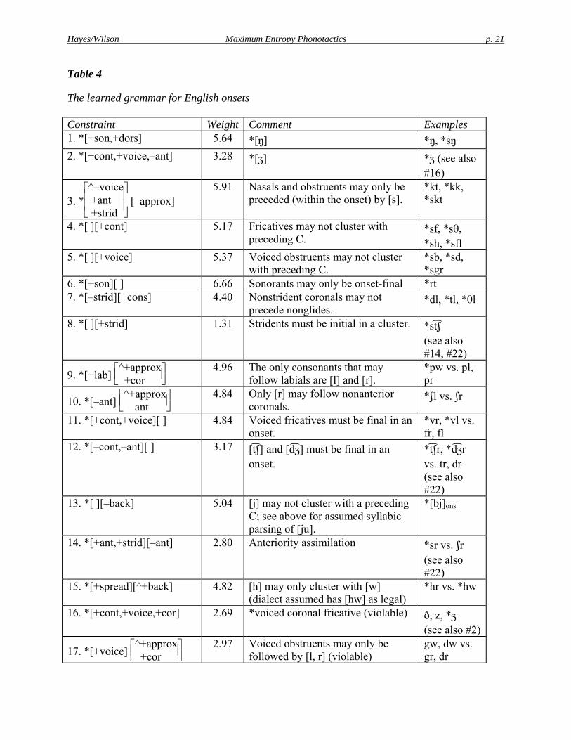
Hayes/Wilson Maximum Entropy Phonotactics p. 21
Table 4
The learned grammar for English onsets
Constraint Weight Comment Examples 1. *[+son,+dors] 5.64 *[ŋ] *ŋ, *sŋ 2. *[+cont,+voice,–ant] 3.28 *[ʒ] *ʒ (see also
#16)
3. *⎣⎢⎢⎡
⎦⎥⎥⎤^–voice
+ant +strid
[–approx] 5.91 Nasals and obstruents may only be
preceded (within the onset) by [s]. *kt, *kk, *skt
4. *[ ][+cont] 5.17 Fricatives may not cluster with preceding C.
*sf, *sθ, *sh, *sfl
5. *[ ][+voice] 5.37 Voiced obstruents may not cluster with preceding C.
*sb, *sd, *sgr
6. *[+son][ ] 6.66 Sonorants may only be onset-final *rt 7. *[–strid][+cons] 4.40 Nonstrident coronals may not
precede nonglides. *dl, *tl, *θl
8. *[ ][+strid] 1.31 Stridents must be initial in a cluster. *stʃ (see also #14, #22)
9. *[+lab] ⎣⎢⎡
⎦⎥⎤^+approx
+cor
4.96 The only consonants that may follow labials are [l] and [r].
*pw vs. pl, pr
10. *[–ant] ⎣⎢⎡
⎦⎥⎤^+approx
–ant 4.84 Only [r] may follow nonanterior
coronals. *ʃl vs. ʃr
11. *[+cont,+voice][ ] 4.84 Voiced fricatives must be final in an onset.
*vr, *vl vs. fr, fl
12. *[–cont,–ant][ ] 3.17 [t ʃ] and [dʒ] must be final in an onset.
*t ʃr, *dʒr vs. tr, dr (see also #22)
13. *[ ][–back] 5.04 [j] may not cluster with a preceding C; see above for assumed syllabic parsing of [ju].
*[bj]ons
14. *[+ant,+strid][–ant] 2.80 Anteriority assimilation *sr vs. ʃr (see also #22)
15. *[+spread][^+back] 4.82 [h] may only cluster with [w] (dialect assumed has [hw] as legal)
*hr vs. *hw
16. *[+cont,+voice,+cor] 2.69 *voiced coronal fricative (violable) ð, z, *ʒ (see also #2)
17. *[+voice] ⎣⎢⎡
⎦⎥⎤^+approx
+cor
2.97 Voiced obstruents may only be followed by [l, r] (violable)
gw, dw vs. gr, dr
Hayes/Wilson Maximum Entropy Phonotactics p. 22
18. *⎣⎢⎡
⎦⎥⎤+cont
–strid ⎣⎢⎡
⎦⎥⎤^+approx
–ant
2.06 [θ, ð] may only be followed by [r] (violable).
θw vs. θr (see also #21)
19. *[ ] ⎣⎢⎢⎡
⎦⎥⎥⎤^–cont
–voice +lab
[+cons] 3.05 In effect: [p] not [k] / s__l
(violable) skl vs. spl
20. *[ ][+cor] ⎣⎢⎡
⎦⎥⎤^+approx
–ant
2.06 In effect: only [r] after [st] ?stw vs. skw, str (see also #23)
21. *[+cont,–strid] 1.84 [θ, ð] are rare (violable). θ vs. f, s 22. *[+strid][–ant] 2.10 In effect: [ʃr] is rare (violable). ʃr vs. fr
23. *⎣⎢⎢⎡
⎦⎥⎥⎤–cont
–voice+cor
⎣⎢⎡
⎦⎥⎤^+approx
–ant
1.70 In effect: [t] can only be followed by [r] (violable).
tw vs. tr
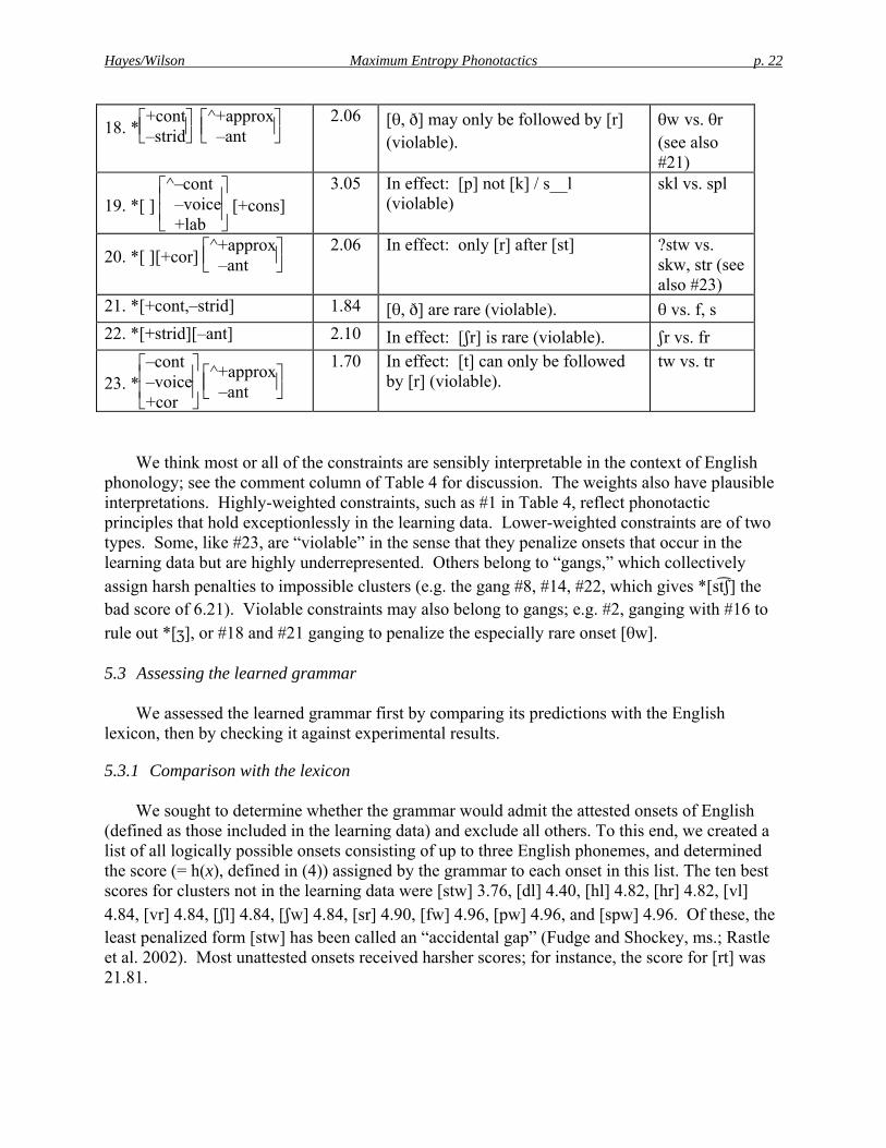
We think most or all of the constraints are sensibly interpretable in the context of English phonology; see the comment column of Table 4 for discussion. The weights also have plausible interpretations. Highly-weighted constraints, such as #1 in Table 4, reflect phonotactic principles that hold exceptionlessly in the learning data. Lower-weighted constraints are of two types. Some, like #23, are “violable” in the sense that they penalize onsets that occur in the learning data but are highly underrepresented. Others belong to “gangs,” which collectively assign harsh penalties to impossible clusters (e.g. the gang #8, #14, #22, which gives *[st ʃ] the bad score of 6.21). Violable constraints may also belong to gangs; e.g. #2, ganging with #16 to rule out *[ʒ], or #18 and #21 ganging to penalize the especially rare onset [θw].
5.3 Assessing the learned grammar
We assessed the learned grammar first by comparing its predictions with the English lexicon, then by checking it against experimental results.
5.3.1 Comparison with the lexicon
We sought to determine whether the grammar would admit the attested onsets of English (defined as those included in the learning data) and exclude all others. To this end, we created a list of all logically possible onsets consisting of up to three English phonemes, and determined the score (= h(x), defined in (4)) assigned by the grammar to each onset in this list. The ten best scores for clusters not in the learning data were [stw] 3.76, [dl] 4.40, [hl] 4.82, [hr] 4.82, [vl] 4.84, [vr] 4.84, [ʃl] 4.84, [ʃw] 4.84, [sr] 4.90, [fw] 4.96, [pw] 4.96, and [spw] 4.96. Of these, the least penalized form [stw] has been called an “accidental gap” (Fudge and Shockey, ms.; Rastle et al. 2002). Most unattested onsets received harsher scores; for instance, the score for [rt] was 21.81.
Hayes/Wilson Maximum Entropy Phonotactics p. 23
Most attested onsets received perfect scores (= 0). However, a few of the rarest onsets did receive penalties: [ð] 4.54, [θw] 3.91, [skl] 3.05, [dw] 2.97, [gw] 2.97, [z] 2.69, [ʃr] 2.10, [θ] 1.85, [θr] 1.85, [tw] 1.70. Given that these onsets are rare ([ð] in particular is illegal except in function words), and that rare real sequences tend to be downrated by native speakers (see §2.3), these scores strike us as plausible.
We conclude that the grammar did a reasonably good job of separating good from bad onsets, the threshold (cf. §3.2) falling at a score of about 4.
5.3.2 Modeling experimental data
We also assessed the grammar on its ability to replicate the gradient judgments of English speakers. To this end we modeled the data from one of the earliest experiments on phonological well-formedness intuitions, Scholes 1966 (Experiment 5). Scholes obtained yes/no ratings of 66 monosyllabic nonwords from a group of seventh grade students (N=33). The students were asked, for each form, whether it “is likely to be usable as a word of English”. The syllable rimes of the nonwords were kept few, and deliberately bland, so that the great bulk of the variation in responses can plausibly be attributed to the onsets. Following Pierrehumbert 1994 and Coleman and Pierrehumbert 1997, we take the proportion of “yes” responses pooled across participants to be an indicator of the mean well-formedness intuition of individuals in the population. Frisch et al. 2000 demonstrate that this method yields scores that are highly correlated with well-formedness ratings on a numerical scale. As with results from similar studies, the pooled Scholes data show a gradient transition from relatively well-formed to highly ill-formed clusters, seen in Figure 3 below.
In assessing the performance of the model against these data, we are comparing probabilities with probabilities; i.e. the probability that an experimental subject will accept the form against the absolute probability assigned to the form by the maxent grammar. For this purpose, we use maxent values (P*(x); (5)), which are proportional to probabilities (6). In addition, we incorporate a free parameter T, whose value is determined on a best-fit basis, and whose purpose is to render the predicted scores comparable in overall distribution to the experimental data.13 Hence, the scores matched against the data are as in (12).
(12) predicted-rating(x) = P*(x)1/T
Under the best fit value (T = 7.4), the correlation of predicted ratings against observed ratings (fraction of “yes” responses) was r = 0.946. This means that most of the variation in the subjects’ responses is explained by the model. The scattergram (Figure 3) shows the predictions of the model plotted against subject ratings for all 62 onsets in the Scholes experiment.
13 T is mnemonic for the computational “temperature,” a term reflecting the origin of maximum entropy theory in statistical mechanics; see e.g. Smolensky 1986:270.

Hayes/Wilson Maximum Entropy Phonotactics p. 24
Figure 3
Performance of the model in predicting the data of Scholes 1966
The correlation of 0.946 becomes more meaningful when compared with the correlations obtained under alternative approaches. We tested five other models, as follows.
I. In order to compare our machine-learned constraints with a hand-crafted grammar, we translated the constraints proposed by Clements and Keyser (1983) into our own formalism and assigned them weights as in §3.3. 14
We also tested four alternatives that are less expressive, in the sense that they do not allow well-formedness to be computed from independent cross-classifying constraints (§2.1).
14 The constraints consisted of numbers 1, 2, 6, 11, 12, 13, and 15 of Table 4, plus *[^–voice,+ant,+strid][+nas], *[^–voice,+ant,+strid][–son], *[+cont,–voice,–ant], [^–cons,+cor], *[+cont][+cont], *[+lab][+lab], *[–strid][+lat], *[–voice,+ant,+strid], [–cons,+cor], *[–voice,+ant,+strid][–cont,–voice,+ant][+back], *[–voice][+voice], and *[ ][–cont,–ant].

Hayes/Wilson Maximum Entropy Phonotactics p. 25
II. The grammar labeled “without features” in Table 5 below was learned in the same way as our model, but differs in having only single-membered natural classes (one per segment in the inventory).
III. We implemented Coleman and Pierrehumbert’s (1997) onset-rhyme model, which has one rule for each onset type in the learning data, and does not use segmental or featural information to relate nonidentical onsets.
IV. We also included an n-gram model from computational linguistics, constructed with the ATT GRM library (Mohri 2002, Allauzen et al. 2005; http://www.research.att.com/sw/tools/grm/). This model uses segmental representations, not features, and was trained with standard methods.
V. Lastly, we tested an analogical model patterned after Bailey and Hahn (2001). This model assesses well-formedness not with grammatical constraints, but on the basis of the aggregate resemblance of the onset under consideration to all the onsets in the learning data.15
All models were fitted to the data with a free parameter T, as with our own model.
The performance (measured by r) of the various models is summarized in Table 5.
Table 5
Comparison of performance of six models 16 Model r our model 0.946 Clements-Keyser constraints with maxent weights 0.936 Coleman and Pierrehumbert 1997 0.893 our model without features 0.885 n-gram model 0.877 analogical model 0.833
As can be seen, our machine-learned grammar was sufficiently accurate that it slightly outperformed a carefully hand-crafted grammar. These two grammars outperform all the others; a plausible reason is they are the only models that employ the standard apparatus of phonological theory, namely features and natural classes.17
15 We explored a number of versions of this model and found that the best-performing version was one that used the segmental similarity metric of Frisch, Pierrehumbert, and Broe 2004 and that paid no heed to token frequencies in the learning data.
16 Because many of the data points were concentrated at the ends of the scale of predicted values, we also performed nonparametric (Spearman) regressions for all of the models. The values corresponding to the rightmost column of Table 5 were 0.889, 0.869, 0.796, 0.757, 0.761, and 0.818.
17 A final note concerning these models. Bailey and Hahn (2001) suggest that improvements in modeling can be obtained if constraint-based and analogical models are blended. We find that this is true, but only to a limited

Hayes/Wilson Maximum Entropy Phonotactics p. 26
We also used the Scholes data to check the consequences of assumptions made in setting up our model. First, we found that the model worked poorly if the search heuristics of §4.2 were dropped. Simply letting the model select constraints at random and weight them yielded poor correlations and failed to separate legal from illegal forms; for example, one run with 1000 randomly selected constraints yielded r = 0.855, with illegal [ŋ lr tl] rated far better than attested [ʃr θw]. Second, the use of implicational constraints (§4.1.1) made a modest difference to the performance of the model; the best grammar learned without implication had 28 (instead of 23) constraints and achieved a correlation of r = 0.926. Finally, the use of token instead of type frequencies for the learning data (fn. 10) also yielded a somewhat lower correlation, r = 0.924 in the best of five runs; for the token frequencies used, see Appendix B.
6. Nonlocal phonotactics: Shona vowel harmony
The English onset simulation was a demonstration of our model in its simple, inductive baseline version. We consider next a phonotactic pattern that requires us to move beyond the baseline. The pattern in question is nonlocal, imposing restrictions on nonadjacent sounds.
Examples of this kind are numerous; we focus here on the vowel harmony system of Shona, a Bantu language of Zimbabwe (Fortune 1955, Beckman 1997, Riggle 1999.) We chose Shona because it has relatively few exceptions in stems, so that vowel harmony is plainly evident as a phonotactic principle. In this respect Shona differs from other vowel harmony languages (see Kiparsky 1973 for Hungarian, Clements and Sezer 1982 for Turkish), where abundant disharmonic stems might create problems for a purely phonotactic learning strategy. For the same reason, we limit our study to verbs, where the harmony pattern is closest to exceptionless.18
6.1 The Shona data pattern
Shona has five vowels: [i e a o u], whose distribution is restricted by the harmony principles given below (examples, given in Shona orthography, are from Hannan 1981):
(13) Shona vowel distribution
a. a is freely distributed.19 b. e, o may occur as follows: i. in initial syllables, as in beka ‘belch’, gondwa ‘become replete with
water’. ii. e may occur noninitially if the preceding vowel is e or o, as in cherenga
‘scratch’, fovedza ‘dent’.
extent. Using the base model augmented by the analogical model, the values corresponding to the rightmost column of Table 5 (first five values) are 0.947, 0.939, 0.923, 0.916, and 0.901.
18 For the idea that particular parts of speech have special phonotactics, see Kelly 1991, Smith 2001. 19 However, in our learning data, final vowels are always /a/, since the dictionary entries for verbs all end
with the suffix /-a/.
Hayes/Wilson Maximum Entropy Phonotactics p. 27
iii. o may occur noninitially only if the preceding vowel is o, as in dokonya ‘be very talkative’.
c. i, u may occur as follows. i. in initial syllables, as in gwisha ‘take away’, huna ‘search intently’. ii. i may occur noninitially unless the preceding vowel is e or o, as in kabida
‘lap (liquid)’, bhigidza ‘hit with thrown object’, churidza ‘plunge, dip’. iii. u may occur noninitially unless the preceding vowel is o, as in baduka
‘split’, bikura ‘snatch and carry away’, chevhura ‘cut deeply with sharp instrument’, dhuguka ‘cook for a long time’.
In dynamic terms, this implies a kind of asymmetrical harmony for [high]: the mid vowels e, o require a following high i to be lowered to e, and the mid vowel o requires a following u to be lowered to o. In fact, Shona suffixes alternate in height in order to remain in conformity with these requirements (Fortune 1955:26, Beckman 1997:10-11), though our focus is on harmony as a phonotactic pattern.
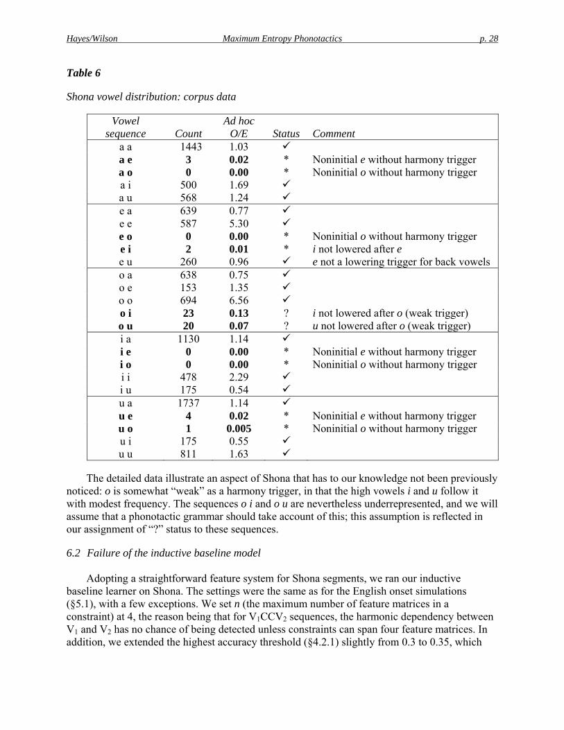
We analyzed 4399 Shona verbs from the online version of Hannan’s (1959) Shona dictionary, available from the CBOLD project (http://www.cbold.ddl.ish-lyon.cnrs.fr/). Inspection of the corpus showed that even in verbs, the harmony system is not free of exceptions: a fair number of idiophones and borrowings violate the normal harmony pattern. The details are given in Table 6, which gives totals from our training set for all 25 possible two-vowel sequences. The table gives both the raw counts and an ad hoc O/E estimate, namely the raw frequency divided by the product of the two individual vowel frequencies. The latter depicts underrepresentation more clearly by compensating for the overall frequencies of vowels. Phonotactically aberrant cases are classified intuitively as “ ”, “?”, or “*” according to the kind of violation they contain.
Hayes/Wilson Maximum Entropy Phonotactics p. 28
Table 6
Shona vowel distribution: corpus data
Vowel sequence Count
Ad hoc O/E
Status Comment
a a 1443 1.03 a e 3 0.02 * Noninitial e without harmony trigger a o 0 0.00 * Noninitial o without harmony trigger a i 500 1.69 a u 568 1.24 e a 639 0.77 e e 587 5.30 e o 0 0.00 * Noninitial o without harmony trigger e i 2 0.01 * i not lowered after e e u 260 0.96 e not a lowering trigger for back vowels o a 638 0.75 o e 153 1.35 o o 694 6.56 o i 23 0.13 ? i not lowered after o (weak trigger) o u 20 0.07 ? u not lowered after o (weak trigger) i a 1130 1.14 i e 0 0.00 * Noninitial e without harmony trigger i o 0 0.00 * Noninitial o without harmony trigger i i 478 2.29 i u 175 0.54 u a 1737 1.14 u e 4 0.02 * Noninitial e without harmony trigger u o 1 0.005 * Noninitial o without harmony trigger u i 175 0.55 u u 811 1.63
The detailed data illustrate an aspect of Shona that has to our knowledge not been previously noticed: o is somewhat “weak” as a harmony trigger, in that the high vowels i and u follow it with modest frequency. The sequences o i and o u are nevertheless underrepresented, and we will assume that a phonotactic grammar should take account of this; this assumption is reflected in our assignment of “?” status to these sequences.
6.2 Failure of the inductive baseline model
Adopting a straightforward feature system for Shona segments, we ran our inductive baseline learner on Shona. The settings were the same as for the English onset simulations (§5.1), with a few exceptions. We set n (the maximum number of feature matrices in a constraint) at 4, the reason being that for V1CCV2 sequences, the harmonic dependency between V1 and V2 has no chance of being detected unless constraints can span four feature matrices. In addition, we extended the highest accuracy threshold (§4.2.1) slightly from 0.3 to 0.35, which
Hayes/Wilson Maximum Entropy Phonotactics p. 29
(ultimately) proved necessary for capturing the marginal status of o u and o i. We ran the learner for several days, forming a grammar of 300 constraints.
To test this grammar, we gave it 50 test words to rate. Of these, 25 took the form mVmVma, where the two slots labeled “V” were filled with all possible vowel pairs (mimima, mimema, etc.) The remaining 25 were similar, but took the form mVndVma, chosen to test if the system had learned the harmonic restrictions across consonant clusters.
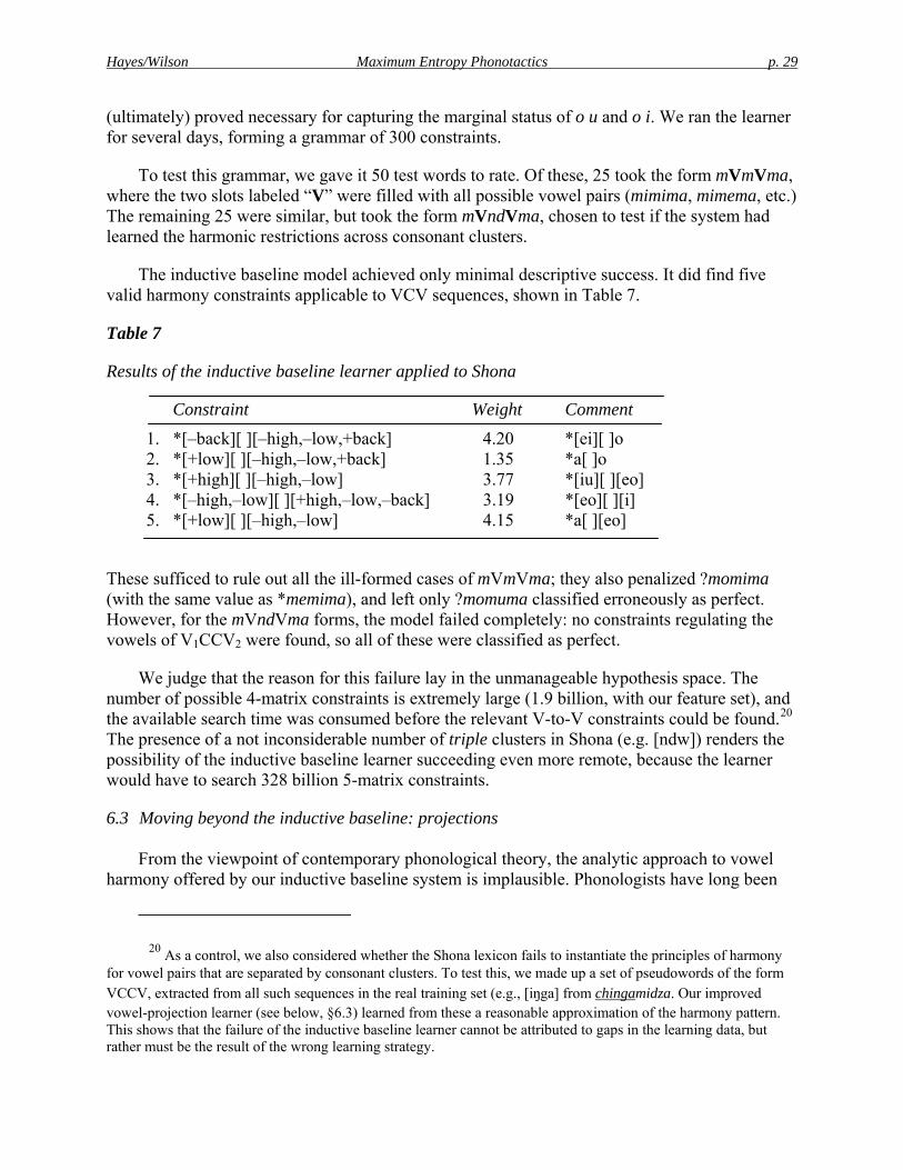
The inductive baseline model achieved only minimal descriptive success. It did find five valid harmony constraints applicable to VCV sequences, shown in Table 7.
Table 7
Results of the inductive baseline learner applied to Shona
Constraint Weight Comment
1. *[–back][ ][–high,–low,+back] 4.20 *[ei][ ]o 2. *[+low][ ][–high,–low,+back] 1.35 *a[ ]o 3. *[+high][ ][–high,–low] 3.77 *[iu][ ][eo] 4. *[–high,–low][ ][+high,–low,–back] 3.19 *[eo][ ][i] 5. *[+low][ ][–high,–low] 4.15 *a[ ][eo]
These sufficed to rule out all the ill-formed cases of mVmVma; they also penalized ?momima (with the same value as *memima), and left only ?momuma classified erroneously as perfect. However, for the mVndVma forms, the model failed completely: no constraints regulating the vowels of V1CCV2 were found, so all of these were classified as perfect.
We judge that the reason for this failure lay in the unmanageable hypothesis space. The number of possible 4-matrix constraints is extremely large (1.9 billion, with our feature set), and the available search time was consumed before the relevant V-to-V constraints could be found.20 The presence of a not inconsiderable number of triple clusters in Shona (e.g. [ndw]) renders the possibility of the inductive baseline learner succeeding even more remote, because the learner would have to search 328 billion 5-matrix constraints.
6.3 Moving beyond the inductive baseline: projections
From the viewpoint of contemporary phonological theory, the analytic approach to vowel harmony offered by our inductive baseline system is implausible. Phonologists have long been
20 As a control, we also considered whether the Shona lexicon fails to instantiate the principles of harmony for vowel pairs that are separated by consonant clusters. To test this, we made up a set of pseudowords of the form VCCV, extracted from all such sequences in the real training set (e.g., [iŋga] from chingamidza. Our improved vowel-projection learner (see below, §6.3) learned from these a reasonable approximation of the harmony pattern. This shows that the failure of the inductive baseline learner cannot be attributed to gaps in the learning data, but rather must be the result of the wrong learning strategy.
Hayes/Wilson Maximum Entropy Phonotactics p. 30
aware that vowel harmony systems normally “care” only about the vowels of the string, and have adopted formal devices that permit this, expressing the nonlocal process in local terms. This can be done, for instance, with an autosegmental tier for vowels (Clements 1976, Goldsmith 1979), perhaps incorporated into some conception of feature geometry (Archangeli and Pulleyblank 1987, Clements and Hume 1995). Without attempting to choose between these theories, we argue that a vocalic representation offers a solution to the problem of learning harmony systems.
To create the effects of a vowel tier in our system, we use the idea of projection (Vergnaud 1977, McCarthy 1979). In particular, the vowel projection of a phonological representation is the substring consisting of all and only its vowels, appearing in the same order as in the main representation. Projections are scanned during constraint discovery in the same way as the full representation, and every constraint applies on its own projection. For example, the constraint *[–high, –low][+high], as defined on the vowel projection, forbids mid-high vowel sequences irrespective of how many consonants intervene.
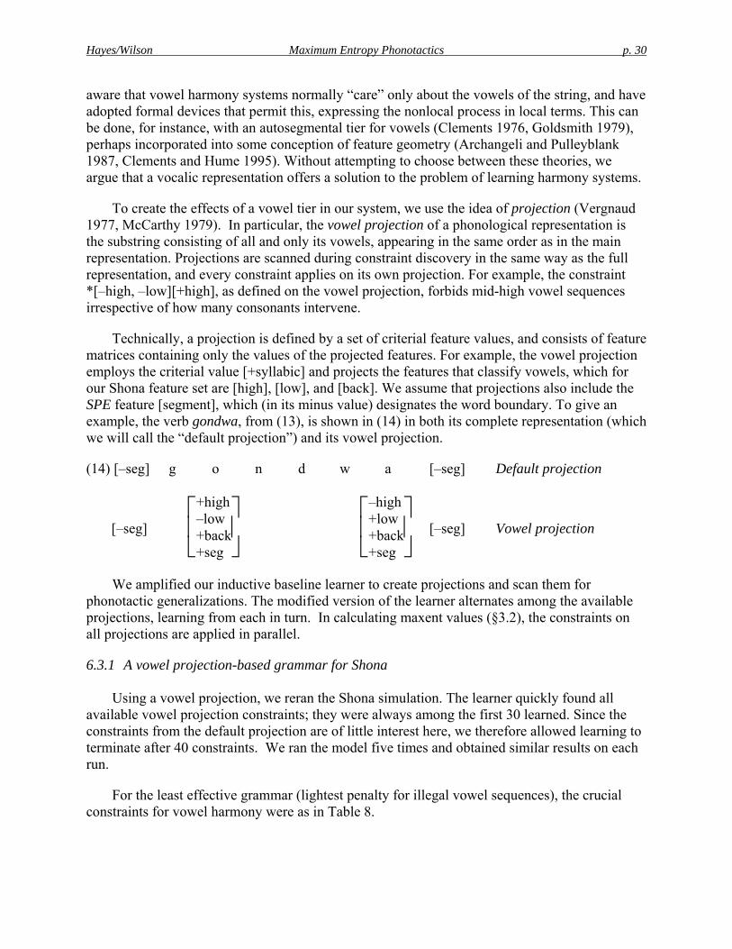
Technically, a projection is defined by a set of criterial feature values, and consists of feature matrices containing only the values of the projected features. For example, the vowel projection employs the criterial value [+syllabic] and projects the features that classify vowels, which for our Shona feature set are [high], [low], and [back]. We assume that projections also include the SPE feature [segment], which (in its minus value) designates the word boundary. To give an example, the verb gondwa, from (13), is shown in (14) in both its complete representation (which we will call the “default projection”) and its vowel projection.
(14) [–seg] g o n d w a [–seg] Default projection
[–seg] ⎣⎢⎡
⎦⎥⎤+high
–low+back+seg
⎣⎢⎡
⎦⎥⎤–high
+low+back+seg
[–seg] Vowel projection
We amplified our inductive baseline learner to create projections and scan them for phonotactic generalizations. The modified version of the learner alternates among the available projections, learning from each in turn. In calculating maxent values (§3.2), the constraints on all projections are applied in parallel.
6.3.1 A vowel projection-based grammar for Shona
Using a vowel projection, we reran the Shona simulation. The learner quickly found all available vowel projection constraints; they were always among the first 30 learned. Since the constraints from the default projection are of little interest here, we therefore allowed learning to terminate after 40 constraints. We ran the model five times and obtained similar results on each run.
For the least effective grammar (lightest penalty for illegal vowel sequences), the crucial constraints for vowel harmony were as in Table 8.
Hayes/Wilson Maximum Entropy Phonotactics p. 31
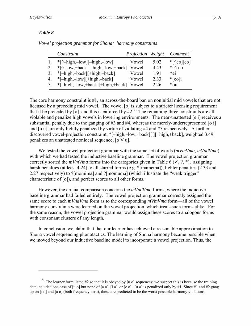
Table 8
Vowel projection grammar for Shona: harmony constraints
Constraint Projection Weight Comment
1. *[^–high,–low][–high,–low] Vowel 5.02 *[^eo][eo] 2. *[^–low,+back][–high,–low,+back] Vowel 4.43 *[^o]o 3. *[–high,–back][+high,–back] Vowel 1.91 *ei 4. *[–high,–low][+high,–back] Vowel 2.33 *[eo]i 5. *[–high,–low,+back][+high,+back] Vowel 2.26 *ou
The core harmony constraint is #1, an across-the-board ban on noninitial mid vowels that are not licensed by a preceding mid vowel. The vowel [o] is subject to a stricter licensing requirement that it be preceded by [o], and this is enforced by #2.21 The remaining three constraints are all violable and penalize high vowels in lowering environments. The near-unattested [e i] receives a substantial penalty due to the ganging of #3 and #4, whereas the merely-underrepresented [o i] and [o u] are only lightly penalized by virtue of violating #4 and #5 respectively. A further discovered vowel-projection constraint, *[–high,–low,+back][ ][+high,+back], weighted 3.49, penalizes an unattested nonlocal sequence, [o V u].
We tested the vowel projection grammar with the same set of words (mVmVma, mVndVma) with which we had tested the inductive baseline grammar. The vowel projection grammar correctly sorted the mVmVma forms into the categories given in Table 6 ( , ?, *), assigning harsh penalties (at least 4.24) to all starred forms (e.g. *[mamema]), lighter penalties (2.33 and 2.27 respectively) to ?[momima] and ?[momuma] (which illustrate the “weak trigger” characteristic of [o]), and perfect scores to all other forms.
However, the crucial comparison concerns the mVndVma forms, where the inductive baseline grammar had failed entirely. The vowel projection grammar correctly assigned the same score to each mVndVma form as to the corresponding mVmVma form—all of the vowel harmony constraints were learned on the vowel projection, which treats such forms alike. For the same reason, the vowel projection grammar would assign these scores to analogous forms with consonant clusters of any length.
In conclusion, we claim that that our learner has achieved a reasonable approximation to Shona vowel sequencing phonotactics. The learning of Shona harmony became possible when we moved beyond our inductive baseline model to incorporate a vowel projection. Thus, the
21 The learner formulated #2 so that it is obeyed by [u o] sequences; we suspect this is because the training data included one case of [u o] but none of [a o], [i o], or [e o]. [u o] is penalized only by #1. Since #1 and #2 gang up on [i o] and [a o] (both frequency zero), these are predicted to be the worst possible harmony violations.
Hayes/Wilson Maximum Entropy Phonotactics p. 32
concept of a vowel tier can be defended on learnability grounds: in controlled comparative simulations, it makes phonotactic learning possible where it would not otherwise be so. 22
7. Locality in stress patterns: the metrical grid
Another type of nonlocal phonotactics is found in stress systems. Where stress is predictable, it is often analyzed derivationally: a grammar assigns a stress contour to each form, based on its segmental or syllabic representation. But predictable stress is also a phonotactic pattern, a regularity of surface forms. We adopt this perspective here, noting that it readily extends to languages like English (Selkirk 1980b) where stress is not fully predictable, but obeys important restrictions.
7.1 Unbounded stress
The locality of stress is seen clearly in so-called unbounded stress patterns. One such pattern, attributed to Eastern Cheremis and various other languages (Hayes 1995:§7.2), works as follows:
(15) a. Every heavy syllable bears some degree of stress. b. Every initial syllable bears some degree of stress. c. Of the stressed syllables in a word, the rightmost bears main stress.
In terms of main stress, this is a “default to opposite” system (Prince 1985), with the pattern “rightmost heavy, else initial.” The generalization in (15c) has been called “End Rule Right” (Prince 1983), a term we will use below.
This description implies two clear instances of nonlocality. First, the fact that exactly one syllable bears main stress (“culminativity”; Hayes 1995) is a nonlocal observation that cannot be stated in our inductive baseline model. Because our model imposes a limit n on the number of feature matrices that may appear in a constraint (§4.1.2), it can only require that the main stress appear within n – 1 syllables of a particular word edge or other landmark; it cannot quantify over all syllables of a word to determine that exactly one of them bears main stress. The same considerations imply that the End Rule Right restriction in (15c) cannot be captured by our inductive baseline learner; there is no guarantee that this syllable will fall within the n-syllable limit.
22 Our reviewers asked if we could dispense with projections and use Kleene-star notation (i.e. (x)*, “zero or more x”) instead. For example, Table 8, #1 would be stated to rule out [^–high,–low] ([^+syllabic])*[–high,–low]. We are skeptical that this would work. Kleene-star is much less restrictive than projections, as it need not employ the same intervention class throughout a constraint. We judge that this would lead to severe search space problems. For example, the constraint of Hungarian that Hayes and Londe (2006) call LOCAL NN is stated by them as *[–back][–back][+back] on a vowel tier; in Kleene-star notation it would require [–back]([–syllabic])*[–back]([–syllabic])*[+back]. With any reasonably large number of natural classes, five-matrix constraints lead to a very large search space.
In general, however, work pursuing the inductive baseline approach must be prepared to consider multiple approaches to solving a learnability problem. The result in this section shows the sufficiency of vowel projections for the task at hand, but to demonstrate necessity would be a long-term project.
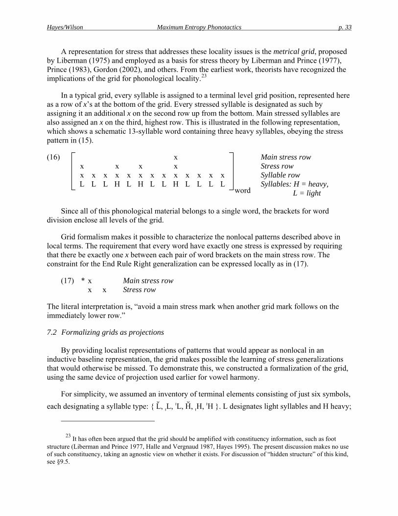
Hayes/Wilson Maximum Entropy Phonotactics p. 33
A representation for stress that addresses these locality issues is the metrical grid, proposed by Liberman (1975) and employed as a basis for stress theory by Liberman and Prince (1977), Prince (1983), Gordon (2002), and others. From the earliest work, theorists have recognized the implications of the grid for phonological locality.23
In a typical grid, every syllable is assigned to a terminal level grid position, represented here as a row of x’s at the bottom of the grid. Every stressed syllable is designated as such by assigning it an additional x on the second row up from the bottom. Main stressed syllables are also assigned an x on the third, highest row. This is illustrated in the following representation, which shows a schematic 13-syllable word containing three heavy syllables, obeying the stress pattern in (15).
(16) x Main stress row x x x x Stress row x x x x x x x x x x x x x Syllable row L L L H L H L L H L L L L Syllables: H = heavy,
word L = light
Since all of this phonological material belongs to a single word, the brackets for word division enclose all levels of the grid.
Grid formalism makes it possible to characterize the nonlocal patterns described above in local terms. The requirement that every word have exactly one stress is expressed by requiring that there be exactly one x between each pair of word brackets on the main stress row. The constraint for the End Rule Right generalization can be expressed locally as in (17).
(17) * x Main stress row x x Stress row
The literal interpretation is, “avoid a main stress mark when another grid mark follows on the immediately lower row.”
7.2 Formalizing grids as projections
By providing localist representations of patterns that would appear as nonlocal in an inductive baseline representation, the grid makes possible the learning of stress generalizations that would otherwise be missed. To demonstrate this, we constructed a formalization of the grid, using the same device of projection used earlier for vowel harmony.
For simplicity, we assumed an inventory of terminal elements consisting of just six symbols, each designating a syllable type: L , ˌL, ˈL, H , ˌH, ˈH . L designates light syllables and H heavy;
23 It has often been argued that the grid should be amplified with constituency information, such as foot structure (Liberman and Prince 1977, Halle and Vergnaud 1987, Hayes 1995). The present discussion makes no use of such constituency, taking an agnostic view on whether it exists. For discussion of “hidden structure” of this kind, see §9.5.

Hayes/Wilson Maximum Entropy Phonotactics p. 34
and the IPA diacritics [ ˌ ˈ ] designate stressless, secondary stressed, and main stressed syllables. These six entities were classified with the prosodic features [heavy], [stress], and [main]: primary stress is [+stress, +main] and secondary stress is [+stress, –main]. We used these features (plus the SPE feature [segment], which distinguishes segments from word boundaries) to express the grid as a set of projections, as in Table 9.
Table 9
Formalizing a metrical grid with projections
Criterial features Projected features
a. Main projection [+main] [segment] b. Stress projection [+stress] [segment], [main] c. Default projection none all
The three projections are shown in detail for a schematic form in (18).
(18) Representing a grid with projections: [ˌL L ˈH L]
[ ]–seg [ ]+seg [ ]–seg Mainprojection
[ ]–seg ⎣⎢⎡
⎦⎥⎤+seg
–main ⎣⎢⎡
⎦⎥⎤+seg
+main [ ]–seg Stressprojection
[ ]–seg ⎣⎢⎡
⎦⎥⎤+seg
–heavy+stress–main
⎣⎢⎡
⎦⎥⎤+seg
–heavy–stress–main
⎣⎢⎡
⎦⎥⎤+seg
+heavy+stress+main
⎣⎢⎡
⎦⎥⎤+seg
–heavy–stress–main
[ ]–seg Defaultprojection
This representation is closely analogous to a traditional grid, as can be seen if one simply replaces every matrix containing [+seg] with x and marks word boundaries with brackets, as shown in (19).
(19) x Main stress row x x Stress row x x x x Syllable row L L H L
word
The projection version may appear to be richer in information, since each row encodes the presence of higher level grid marks with its featural content. However, traditional use of grids has generally done more or less the same, relying on geometrical (“dominated by”) rather than featural descriptions.
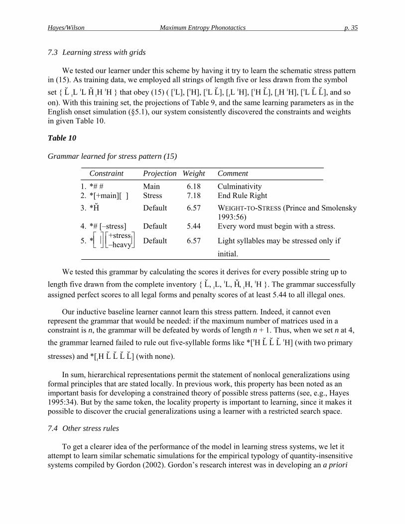
Hayes/Wilson Maximum Entropy Phonotactics p. 35
7.3 Learning stress with grids
We tested our learner under this scheme by having it try to learn the schematic stress pattern in (15). As training data, we employed all strings of length five or less drawn from the symbol set L ˌL ˈL H ˌH ˈH that obey (15) ( [ˈL], [ˈH], [ˈL L], [ˌL ˈH], [ˈH L], [ˌH ˈH], [ˈL L L], and so on). With this training set, the projections of Table 9, and the same learning parameters as in the English onset simulation (§5.1), our system consistently discovered the constraints and weights in given Table 10.
Table 10
Grammar learned for stress pattern (15)
Constraint Projection Weight Comment
1. *# # Main 6.18 Culminativity 2. *[+main][ ] Stress 7.18 End Rule Right 3. *H Default 6.57 WEIGHT-TO-STRESS (Prince and Smolensky
1993:56) 4. *# [–stress] Default 5.44 Every word must begin with a stress.
5. *⎣⎢⎡⎦⎥⎤
⎣⎢⎡
⎦⎥⎤+stress
–heavy Default 6.57 Light syllables may be stressed only if
initial. We tested this grammar by calculating the scores it derives for every possible string up to
length five drawn from the complete inventory L , ˌL, ˈL, H, ˌH, ˈH . The grammar successfully assigned perfect scores to all legal forms and penalty scores of at least 5.44 to all illegal ones.
Our inductive baseline learner cannot learn this stress pattern. Indeed, it cannot even represent the grammar that would be needed: if the maximum number of matrices used in a constraint is n, the grammar will be defeated by words of length n + 1. Thus, when we set n at 4, the grammar learned failed to rule out five-syllable forms like *[ˈH L L L ˈH] (with two primary
stresses) and *[ˌH L L L L] (with none).
In sum, hierarchical representations permit the statement of nonlocal generalizations using formal principles that are stated locally. In previous work, this property has been noted as an important basis for developing a constrained theory of possible stress patterns (see, e.g., Hayes 1995:34). But by the same token, the locality property is important to learning, since it makes it possible to discover the crucial generalizations using a learner with a restricted search space.
7.4 Other stress rules
To get a clearer idea of the performance of the model in learning stress systems, we let it attempt to learn similar schematic simulations for the empirical typology of quantity-insensitive systems compiled by Gordon (2002). Gordon’s research interest was in developing an a priori
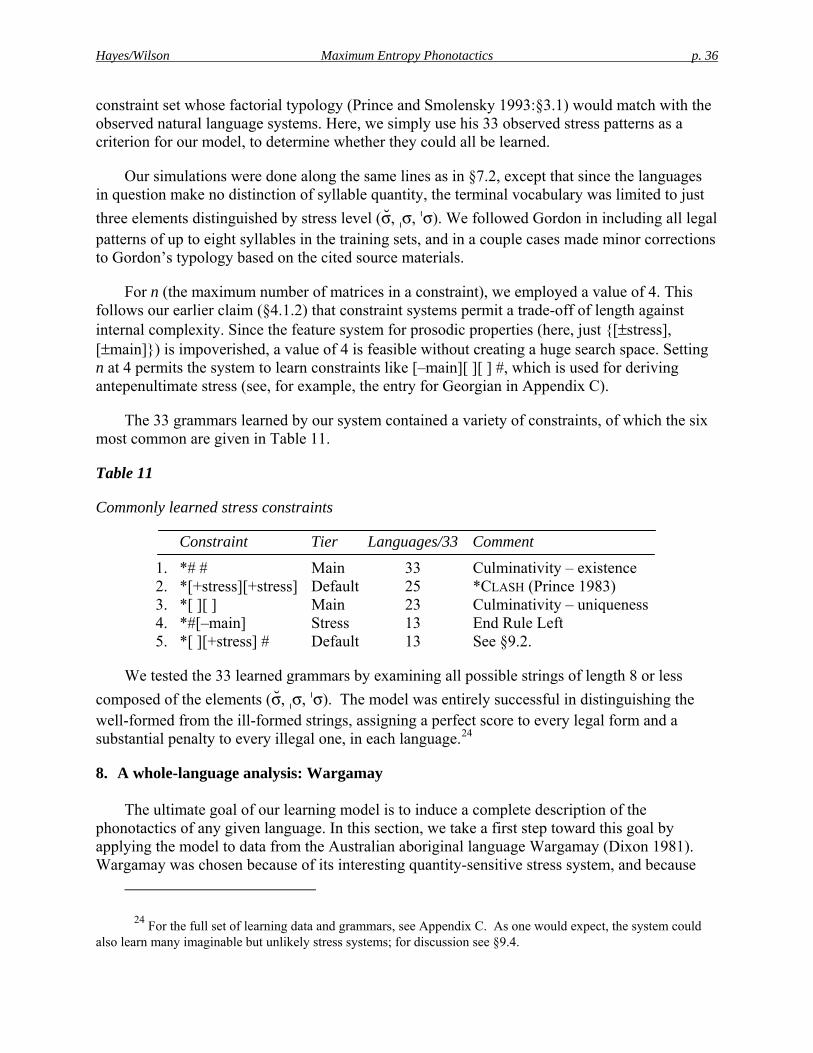
Hayes/Wilson Maximum Entropy Phonotactics p. 36
constraint set whose factorial typology (Prince and Smolensky 1993:§3.1) would match with the observed natural language systems. Here, we simply use his 33 observed stress patterns as a criterion for our model, to determine whether they could all be learned.
Our simulations were done along the same lines as in §7.2, except that since the languages in question make no distinction of syllable quantity, the terminal vocabulary was limited to just three elements distinguished by stress level (σ, ˌσ, ˈσ). We followed Gordon in including all legal patterns of up to eight syllables in the training sets, and in a couple cases made minor corrections to Gordon’s typology based on the cited source materials.
For n (the maximum number of matrices in a constraint), we employed a value of 4. This follows our earlier claim (§4.1.2) that constraint systems permit a trade-off of length against internal complexity. Since the feature system for prosodic properties (here, just [±stress], [±main]) is impoverished, a value of 4 is feasible without creating a huge search space. Setting n at 4 permits the system to learn constraints like [–main][ ][ ] #, which is used for deriving antepenultimate stress (see, for example, the entry for Georgian in Appendix C).
The 33 grammars learned by our system contained a variety of constraints, of which the six most common are given in Table 11.
Table 11
Commonly learned stress constraints
Constraint Tier Languages/33 Comment
1. *# # Main 33 Culminativity – existence 2. *[+stress][+stress] Default 25 *CLASH (Prince 1983) 3. *[ ][ ] Main 23 Culminativity – uniqueness 4. *#[–main] Stress 13 End Rule Left 5. *[ ][+stress] # Default 13 See §9.2.
We tested the 33 learned grammars by examining all possible strings of length 8 or less composed of the elements (σ, ˌσ, ˈσ). The model was entirely successful in distinguishing the well-formed from the ill-formed strings, assigning a perfect score to every legal form and a substantial penalty to every illegal one, in each language.24
8. A whole-language analysis: Wargamay
The ultimate goal of our learning model is to induce a complete description of the phonotactics of any given language. In this section, we take a first step toward this goal by applying the model to data from the Australian aboriginal language Wargamay (Dixon 1981). Wargamay was chosen because of its interesting quantity-sensitive stress system, and because
24 For the full set of learning data and grammars, see Appendix C. As one would expect, the system could also learn many imaginable but unlikely stress systems; for discussion see §9.4.
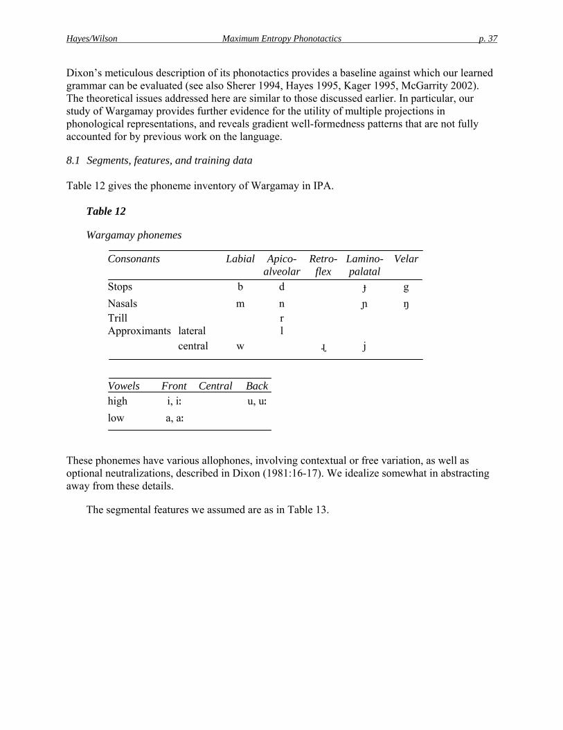
Hayes/Wilson Maximum Entropy Phonotactics p. 37
Dixon’s meticulous description of its phonotactics provides a baseline against which our learned grammar can be evaluated (see also Sherer 1994, Hayes 1995, Kager 1995, McGarrity 2002). The theoretical issues addressed here are similar to those discussed earlier. In particular, our study of Wargamay provides further evidence for the utility of multiple projections in phonological representations, and reveals gradient well-formedness patterns that are not fully accounted for by previous work on the language.
8.1 Segments, features, and training data
Table 12 gives the phoneme inventory of Wargamay in IPA.
Table 12
Wargamay phonemes
Consonants Labial Apico- Retro- Lamino- Velar alveolar flex palatal Stops b d ɟ g Nasals m n ɲ ŋ Trill r Approximants lateral l central w ɻ j Vowels Front Central Back high i, iː u, uː
low a, aː
These phonemes have various allophones, involving contextual or free variation, as well as optional neutralizations, described in Dixon (1981:16-17). We idealize somewhat in abstracting away from these details.
The segmental features we assumed are as in Table 13.

Hayes/Wilson Maximum Entropy Phonotactics p. 38
Table 13
Feature chart for Wargamay
b d ɟ g m n ɲ ŋ r l ɻ j w i a u iː aː uː syl – – – – – – – – – – – – – + + + + + + cons + + + + + + + + + + + – – – – – – – – approx – – – – – – – – + + + + + + + + + + + son – – – – + + + + + + + + + + + + + + + lab + + cor + + + + + + + ant + – + – + + – lat – + – dors + + high + + + – + + – + back – + – + + – + + long – – – + + +
In addition, we assumed that vowels are classified by the prosodic features [stress] and [main], as in §7.2.
We used as our learning data the vocabulary of approximately 950 items included in Dixon’s grammar. We removed reduplicated forms, which Dixon treats as two separate phonological words, and a handful of forms that contain blatant violations of the phonotactic system.25
The set of remaining forms was considerably smaller than the learning data for our previous analyses and contained only one item of more than four syllables. We judged this corpus to be too limited to serve as input to our learner, particularly because we are interested in learning the stress system of the language. Therefore, we inflected each nominal and verbal root according to the morphological description given by Dixon (1981:27ff.). The resulting set contains about 6000 words and instantiates the stress pattern across a range of word lengths from one to six syllables. In the following sections, we discuss how the grammar learned from these data accounts for the segmental and stress phonotactics of Wargamay.
8.2 Learning simulation
The resources our learner used for Wargamay integrate those from the previous sections. We deployed projections for a metrical grid (as in (18)) as well as a vowel projection (§6.3).26
Our
25 These are [ŋijaɲma] ‘ask’ ([ɲm] cluster), [jawujɲbaɻi] ‘big grey kangaroo’ ([jɲb] cluster, with the phonotactically-regular variant [jawujmbaɻi]), and the loanwords [drajga] ‘tracker’ (initial cluster), [gaːguɻuɟ] ‘cockroach’ (final obstruent), and [lajn] ‘line’ (initial [l] and final cluster).
26 As it happened, no constraints were learned on the Vowel projection. However, assuming that projections are not learned on a language-specific basis, but are specified in UG, learners have no choice but to search each one during phonotactic learning.
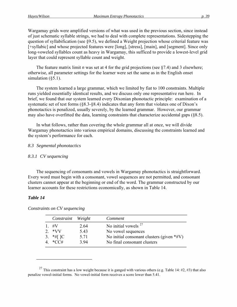
Hayes/Wilson Maximum Entropy Phonotactics p. 39
Wargamay grids were amplified versions of what was used in the previous section, since instead of just schematic syllable strings, we had to deal with complete representations. Sidestepping the question of syllabification (see §9.5), we defined a Weight projection whose criterial feature was [+syllabic] and whose projected features were [long], [stress], [main], and [segment]. Since only long-voweled syllables count as heavy in Wargamay, this sufficed to provide a lowest-level grid layer that could represent syllable count and weight.
The feature matrix limit n was set at 4 for the grid projections (see §7.4) and 3 elsewhere; otherwise, all parameter settings for the learner were set the same as in the English onset simulation (§5.1).
The system learned a large grammar, which we limited by fiat to 100 constraints. Multiple runs yielded essentially identical results, and we discuss only one representative run here. In brief, we found that our system learned every Dixonian phonotactic principle: examination of a systematic set of test forms (§8.3-§8.4) indicates that any form that violates one of Dixon’s phonotactics is penalized, usually severely, by the learned grammar. However, our grammar may also have overfitted the data, learning constraints that characterize accidental gaps (§8.5).
In what follows, rather than covering the whole grammar all at once, we will divide Wargamay phonotactics into various empirical domains, discussing the constraints learned and the system’s performance for each.
8.3 Segmental phonotactics
8.3.1 CV sequencing
The sequencing of consonants and vowels in Wargamay phonotactics is straightforward. Every word must begin with a consonant, vowel sequences are not permitted, and consonant clusters cannot appear at the beginning or end of the word. The grammar constructed by our learner accounts for these restrictions economically, as shown in Table 14.
Table 14
Constraints on CV sequencing
Constraint Weight Comment
1. #V 2.64 No initial vowels 27 2. *VV 5.43 No vowel sequences 3. *#[ ]C 5.71 No initial consonant clusters (given *#V) 4. *CC# 3.94 No final consonant clusters
27 This constraint has a low weight because it is ganged with various others (e.g. Table 14: #2, #3) that also penalize vowel-initial forms. No vowel-initial form receives a score lower than 5.41.
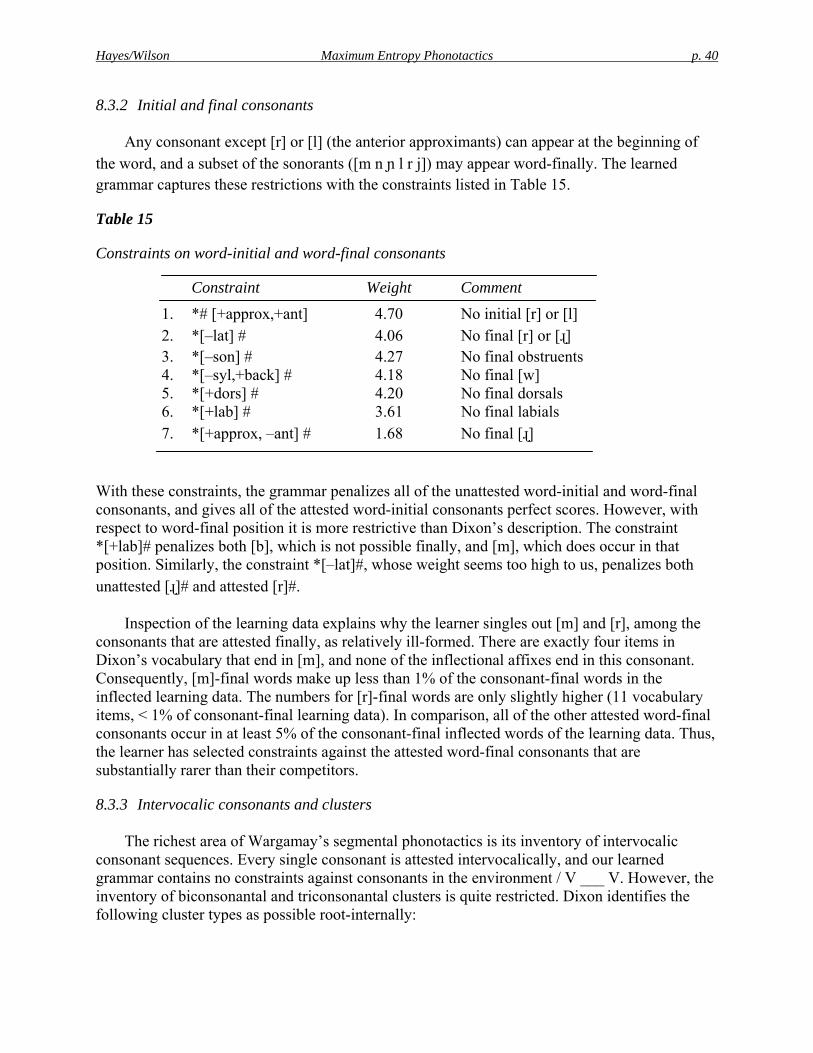
Hayes/Wilson Maximum Entropy Phonotactics p. 40
8.3.2 Initial and final consonants
Any consonant except [r] or [l] (the anterior approximants) can appear at the beginning of the word, and a subset of the sonorants ([m n ɲ l r j]) may appear word-finally. The learned grammar captures these restrictions with the constraints listed in Table 15.
Table 15
Constraints on word-initial and word-final consonants
Constraint Weight Comment
1. *# [+approx,+ant] 4.70 No initial [r] or [l] 2. *[–lat] # 4.06 No final [r] or [ɻ] 3. *[–son] # 4.27 No final obstruents 4. *[–syl,+back] # 4.18 No final [w] 5. *[+dors] # 4.20 No final dorsals 6. *[+lab] # 3.61 No final labials 7. *[+approx, –ant] # 1.68 No final [ɻ]
With these constraints, the grammar penalizes all of the unattested word-initial and word-final consonants, and gives all of the attested word-initial consonants perfect scores. However, with respect to word-final position it is more restrictive than Dixon’s description. The constraint *[+lab]# penalizes both [b], which is not possible finally, and [m], which does occur in that position. Similarly, the constraint *[–lat]#, whose weight seems too high to us, penalizes both unattested [ɻ]# and attested [r]#.
Inspection of the learning data explains why the learner singles out [m] and [r], among the consonants that are attested finally, as relatively ill-formed. There are exactly four items in Dixon’s vocabulary that end in [m], and none of the inflectional affixes end in this consonant. Consequently, [m]-final words make up less than 1% of the consonant-final words in the inflected learning data. The numbers for [r]-final words are only slightly higher (11 vocabulary items, < 1% of consonant-final learning data). In comparison, all of the other attested word-final consonants occur in at least 5% of the consonant-final inflected words of the learning data. Thus, the learner has selected constraints against the attested word-final consonants that are substantially rarer than their competitors.
8.3.3 Intervocalic consonants and clusters
The richest area of Wargamay’s segmental phonotactics is its inventory of intervocalic consonant sequences. Every single consonant is attested intervocalically, and our learned grammar contains no constraints against consonants in the environment / V ___ V. However, the inventory of biconsonantal and triconsonantal clusters is quite restricted. Dixon identifies the following cluster types as possible root-internally:
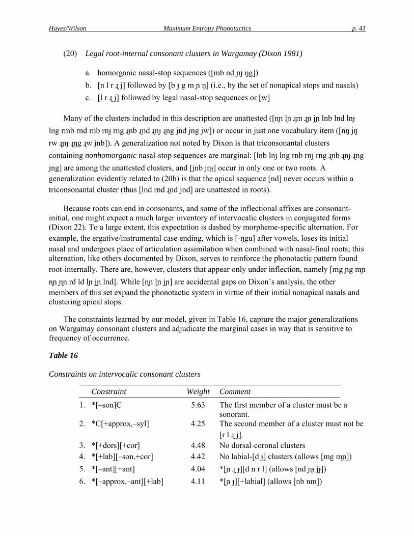
Hayes/Wilson Maximum Entropy Phonotactics p. 41
(20) Legal root-internal consonant clusters in Wargamay (Dixon 1981)
a. homorganic nasal-stop sequences ([mb nd ɲ ŋg]) b. [n l r ɻ j] followed by [b g m ɲ ŋ] (i.e., by the set of nonapical stops and nasals) c. [l r ɻ j] followed by legal nasal-stop sequences or [w]
Many of the clusters included in this description are unattested ([nɲ lɲ ɻm ɻɲ jɲ lnb lnd lnɟ lng rmb rnd rnb rnɟ rng ɻnb ɻnd ɻnɟ ɻng jnd jng jw]) or occur in just one vocabulary item ([nŋ jŋ rw ɻɲɟ ɻŋg ɻw jnb]). A generalization not noted by Dixon is that triconsonantal clusters containing nonhomorganic nasal-stop sequences are marginal: [lnb lnɟ lng rnb rnɟ rng ɻnb ɻnɟ ɻng jng] are among the unattested clusters, and [jnb jnɟ] occur in only one or two roots. A generalization evidently related to (20b) is that the apical sequence [nd] never occurs within a triconsonantal cluster (thus [lnd rnd ɻnd jnd] are unattested in roots).
Because roots can end in consonants, and some of the inflectional affixes are consonant-initial, one might expect a much larger inventory of intervocalic clusters in conjugated forms (Dixon 22). To a large extent, this expectation is dashed by morpheme-specific alternation. For example, the ergative/instrumental case ending, which is [-ŋgu] after vowels, loses its initial nasal and undergoes place of articulation assimilation when combined with nasal-final roots; this alternation, like others documented by Dixon, serves to reinforce the phonotactic pattern found root-internally. There are, however, clusters that appear only under inflection, namely [mg ɲg mɲ nɲ ɲɲ rd ld lɲ jɲ lnd]. While [nɲ lɲ jɲ] are accidental gaps on Dixon’s analysis, the other members of this set expand the phonotactic system in virtue of their initial nonapical nasals and clustering apical stops.
The constraints learned by our model, given in Table 16, capture the major generalizations on Wargamay consonant clusters and adjudicate the marginal cases in way that is sensitive to frequency of occurrence.
Table 16
Constraints on intervocalic consonant clusters
Constraint Weight Comment
1. *[–son]C 5.63 The first member of a cluster must be a sonorant.
2. *C[+approx,–syl] 4.25 The second member of a cluster must not be [r l ɻ j].
3. *[+dors][+cor] 4.48 No dorsal-coronal clusters 4. *[+lab][–son,+cor] 4.42 No labial-[d ɟ] clusters (allows [mg mɲ]) 5. *[–ant][+ant] 4.04 *[ɲ ɻ ɟ][d n r l] (allows [nd ɲɟ jɟ]) 6. *[–approx,–ant][+lab] 4.11 *[ɲ ɟ][+labial] (allows [nb nm])
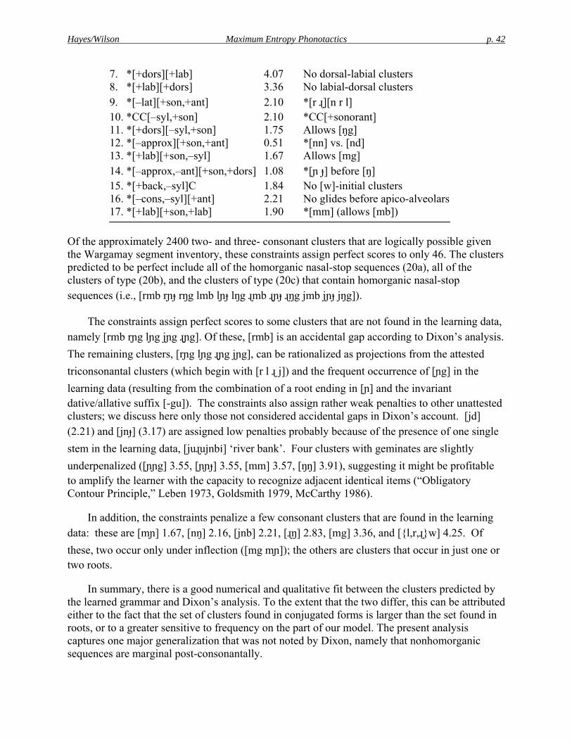
Hayes/Wilson Maximum Entropy Phonotactics p. 42
7. *[+dors][+lab] 4.07 No dorsal-labial clusters 8. *[+lab][+dors] 3.36 No labial-dorsal clusters 9. *[–lat][+son,+ant] 2.10 *[r ɻ][n r l] 10. *CC[–syl,+son] 2.10 *CC[+sonorant] 11. *[+dors][–syl,+son] 1.75 Allows [ŋg] 12. *[–approx][+son,+ant] 0.51 *[nn] vs. [nd] 13. *[+lab][+son,–syl] 1.67 Allows [mg] 14. *[–approx,–ant][+son,+dors] 1.08 *[ɲ ] before [ŋ] 15. *[+back,–syl]C 1.84 No [w]-initial clusters 16. *[–cons,–syl][+ant] 2.21 No glides before apico-alveolars 17. *[+lab][+son,+lab] 1.90 *[mm] (allows [mb])
Of the approximately 2400 two- and three- consonant clusters that are logically possible given the Wargamay segment inventory, these constraints assign perfect scores to only 46. The clusters predicted to be perfect include all of the homorganic nasal-stop sequences (20a), all of the clusters of type (20b), and the clusters of type (20c) that contain homorganic nasal-stop sequences (i.e., [rmb rɲɟ rŋg lmb lɲɟ lŋg ɻmb ɻɲɟ ɻŋg jmb jɲɟ jŋg]).
The constraints assign perfect scores to some clusters that are not found in the learning data, namely [rmb rɲg lɲg jɲg ɻɲg]. Of these, [rmb] is an accidental gap according to Dixon’s analysis. The remaining clusters, [rɲg lɲg ɻɲg jɲg], can be rationalized as projections from the attested triconsonantal clusters (which begin with [r l ɻ j]) and the frequent occurrence of [ɲg] in the learning data (resulting from the combination of a root ending in [ɲ] and the invariant dative/allative suffix [-gu]). The constraints also assign rather weak penalties to other unattested clusters; we discuss here only those not considered accidental gaps in Dixon’s account. [jd] (2.21) and [jnɟ] (3.17) are assigned low penalties probably because of the presence of one single stem in the learning data, [juɻujnbi] ‘river bank’. Four clusters with geminates are slightly underpenalized ([ɲɲg] 3.55, [ɲɲɟ] 3.55, [mm] 3.57, [ŋŋ] 3.91), suggesting it might be profitable to amplify the learner with the capacity to recognize adjacent identical items (“Obligatory Contour Principle,” Leben 1973, Goldsmith 1979, McCarthy 1986).
In addition, the constraints penalize a few consonant clusters that are found in the learning data: these are [mɲ] 1.67, [nŋ] 2.16, [jnb] 2.21, [ɻŋ] 2.83, [mg] 3.36, and [l,r,ɻw] 4.25. Of these, two occur only under inflection ([mg mɲ]); the others are clusters that occur in just one or two roots.
In summary, there is a good numerical and qualitative fit between the clusters predicted by the learned grammar and Dixon’s analysis. To the extent that the two differ, this can be attributed either to the fact that the set of clusters found in conjugated forms is larger than the set found in roots, or to a greater sensitive to frequency on the part of our model. The present analysis captures one major generalization that was not noted by Dixon, namely that nonhomorganic sequences are marginal post-consonantally.

Hayes/Wilson Maximum Entropy Phonotactics p. 43
8.3.4 Consonant-vowel combinations
In comparison to consonant cluster phonotactics, the regularities governing consonant-vowel combinations in Wargamay are understudied. However, Dixon (1981) does note one restriction on VC sequences: [ij] occurs pre-vocalically, but not before a consonant or at the end of the word. Further evidence for this phonotactic comes from the phonological rule of Yotic Deletion
(Dixon 1981: 23), which eliminates [j] in the environment / [i] ___⎩⎨⎧
⎭⎬⎫C
# .
Our model learns three constraints (Table 17) to cover this part of the system.
Table 17
Constraints for yotic deletion
Constraint Weight Comment
1. *[–back,+syl][–cons][^–long,+back] 3.99 *[i][jw]C, *[i][jw][i] 2. *[+high,+syl][^+son,+cor]# 2.88 *[iu]C#, where C ∉ [nɲrlɻ] 3. *[–back,+syl][^+son,+cor]# 1.99 *[i]C#, where C ∉ [nɲrlɻ]
It can be seen that the learner, in its rigorous pursuit of general constraints (§4.2.2), goes beyond Dixon’s narrow description of the [ij] phonotactic. In the learning data, there are no instances of [iw]C (recall that [w] cannot appear in the first position of a consonant cluster), [iji], or [iwi]; the first constraint folds these gaps together with the ban on [ij]C. Similarly, there are only nine roots in the vocabulary that exemplify [uj]#; the second constraint therefore expresses a gradient prohibition on both [ij]# and [uj]#, while the third constraint forms with the second a gang ensuring that unattested [ij]# receives a greater penalty. (The complement class [^+son,+cor] appears in these constraints because it is the largest class that contains all of the legal word-final consonants except [j].)
8.4 Metrical phonotactics
Wargamay stress respects a distinction between heavy and light syllables, where a heavy syllable is defined as one containing a long vowel, irrespective of whether it is closed. Words containing all light syllables exhibit a right-to-left trochaic pattern:
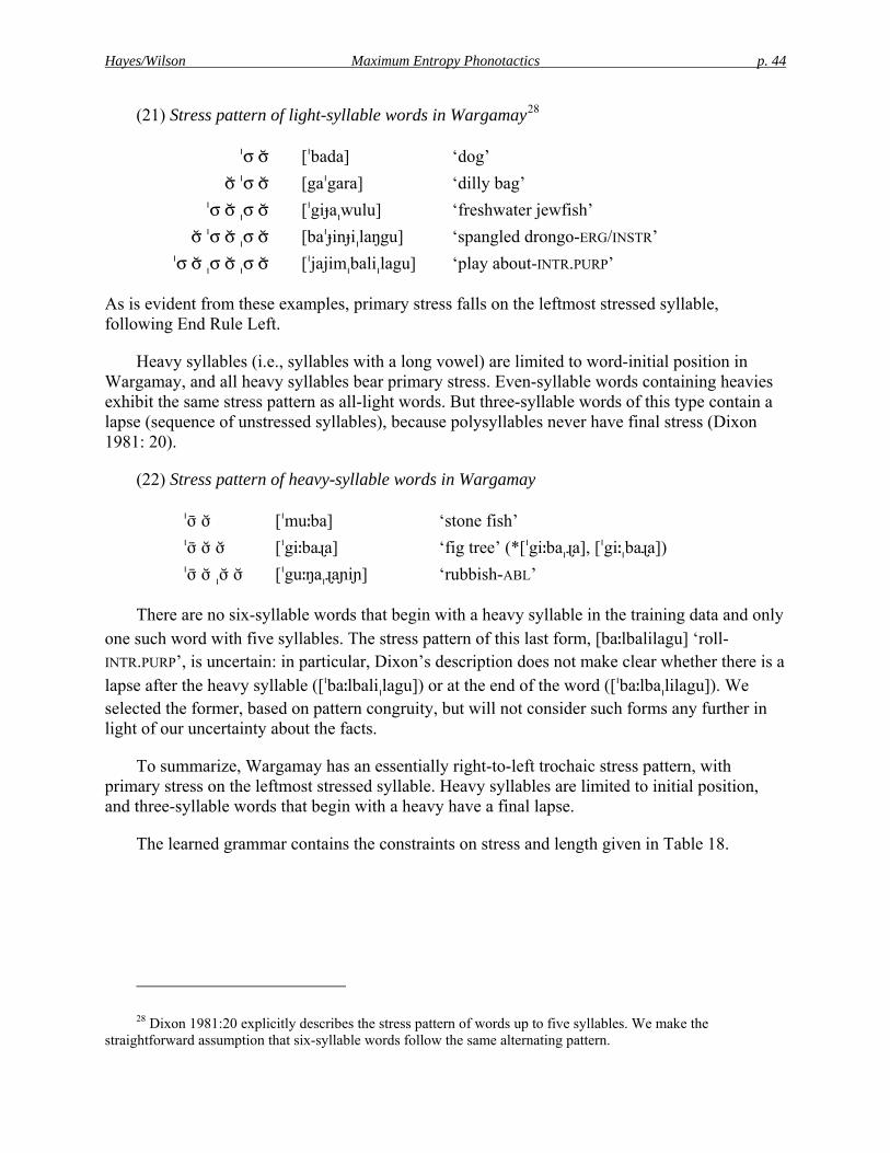
Hayes/Wilson Maximum Entropy Phonotactics p. 44
(21) Stress pattern of light-syllable words in Wargamay28
ˈσ σ [ˈbada] ‘dog’ σ ˈσ σ [gaˈgara] ‘dilly bag’ ˈσ σ ˌσ σ [ˈgiɟaˌwulu] ‘freshwater jewfish’ σ ˈσ σ ˌσ σ [baˈɟinɟiˌlaŋgu] ‘spangled drongo-ERG/INSTR’
ˈσ σ ˌσ σ ˌσ σ [ˈjajimˌbaliˌlagu] ‘play about-INTR.PURP’
As is evident from these examples, primary stress falls on the leftmost stressed syllable, following End Rule Left.
Heavy syllables (i.e., syllables with a long vowel) are limited to word-initial position in Wargamay, and all heavy syllables bear primary stress. Even-syllable words containing heavies exhibit the same stress pattern as all-light words. But three-syllable words of this type contain a lapse (sequence of unstressed syllables), because polysyllables never have final stress (Dixon 1981: 20).
(22) Stress pattern of heavy-syllable words in Wargamay
ˈσ σ [ˈmuːba] ‘stone fish’ ˈσ σ σ [ˈgiːbaɻa] ‘fig tree’ (*[ˈgiːbaˌɻa], [ˈgiːˌbaɻa]) ˈσ σ ˌσ σ [ˈguːŋaˌɻaɲiɲ] ‘rubbish-ABL’
There are no six-syllable words that begin with a heavy syllable in the training data and only one such word with five syllables. The stress pattern of this last form, [baːlbalilagu] ‘roll-INTR.PURP’, is uncertain: in particular, Dixon’s description does not make clear whether there is a lapse after the heavy syllable ([ˈbaːlbaliˌlagu]) or at the end of the word ([ˈbaːlbaˌlilagu]). We selected the former, based on pattern congruity, but will not consider such forms any further in light of our uncertainty about the facts.
To summarize, Wargamay has an essentially right-to-left trochaic stress pattern, with primary stress on the leftmost stressed syllable. Heavy syllables are limited to initial position, and three-syllable words that begin with a heavy have a final lapse.
The learned grammar contains the constraints on stress and length given in Table 18.
28 Dixon 1981:20 explicitly describes the stress pattern of words up to five syllables. We make the straightforward assumption that six-syllable words follow the same alternating pattern.
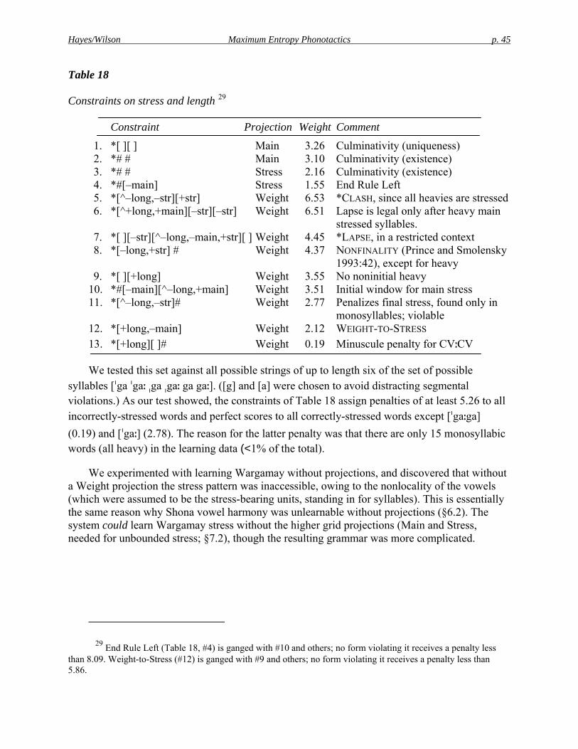
Hayes/Wilson Maximum Entropy Phonotactics p. 45
Table 18
Constraints on stress and length 29
Constraint Projection Weight Comment
1. *[ ][ ] Main 3.26 Culminativity (uniqueness) 2. *# # Main 3.10 Culminativity (existence) 3. *# # Stress 2.16 Culminativity (existence) 4. *#[–main] Stress 1.55 End Rule Left 5. *[^–long,–str][+str] Weight 6.53 *CLASH, since all heavies are stressed 6. *[^+long,+main][–str][–str] Weight 6.51 Lapse is legal only after heavy main
stressed syllables. 7. *[ ][–str][^–long,–main,+str][ ] Weight 4.45 *LAPSE, in a restricted context 8. *[–long,+str] # Weight 4.37 NONFINALITY (Prince and Smolensky
1993:42), except for heavy 9. *[ ][+long] Weight 3.55 No noninitial heavy 10. *#[–main][^–long,+main] Weight 3.51 Initial window for main stress 11. *[^–long,–str]# Weight 2.77 Penalizes final stress, found only in
monosyllables; violable 12. *[+long,–main] Weight 2.12 WEIGHT-TO-STRESS 13. *[+long][ ]# Weight 0.19 Minuscule penalty for CVːCV
We tested this set against all possible strings of up to length six of the set of possible syllables [ˈga ˈgaː ˌga ˌgaː ga gaː]. ([g] and [a] were chosen to avoid distracting segmental violations.) As our test showed, the constraints of Table 18 assign penalties of at least 5.26 to all incorrectly-stressed words and perfect scores to all correctly-stressed words except [ˈgaːga] (0.19) and [ˈgaː] (2.78). The reason for the latter penalty was that there are only 15 monosyllabic words (all heavy) in the learning data (<1% of the total).
We experimented with learning Wargamay without projections, and discovered that without a Weight projection the stress pattern was inaccessible, owing to the nonlocality of the vowels (which were assumed to be the stress-bearing units, standing in for syllables). This is essentially the same reason why Shona vowel harmony was unlearnable without projections (§6.2). The system could learn Wargamay stress without the higher grid projections (Main and Stress, needed for unbounded stress; §7.2), though the resulting grammar was more complicated.
29 End Rule Left (Table 18, #4) is ganged with #10 and others; no form violating it receives a penalty less than 8.09. Weight-to-Stress (#12) is ganged with #9 and others; no form violating it receives a penalty less than 5.86.
Hayes/Wilson Maximum Entropy Phonotactics p. 46
8.5 Additional constraints
The 43 constraints discussed above account for all of the phonotactics of Wargamay discussed by Dixon (1981). The learner also selected 57 additional constraints that have no direct analogue in Dixon’s analysis. A complete list of these constraints appears in Appendix D.
These additional constraints tend to be somewhat complex and unintuitive from a phonologist’s point of view. They either are unviolated in the training data (28 constraints), or are violated only a few times, indicating underrepresentation (29 constraints). All are stated on the default projection; i.e. they are segmental constraints. None is weighted higher than 5.0; in contrast, the learner assigned values over 5 to several highly general, exceptionless constraints listed above.
We have two conjectures for the presence of these puzzling constraints. First, it is possible that they are valid, by which we mean that had it been possible to carry out experiments with Wargamay speakers of the kind Scholes performed, it would have emerged that test forms violating these constraints were rated low. Another possibility, however, is that our learner overfitted the data, seizing on generalizations that are accidentally true. If this is the case (as parallel study of living languages could reveal), there are two possible responses.
One would seek phonology-independent measures of grammar complexity that would limited the number of constraints learned. We note that the last “Dixonian” constraint in our grammar (ignoring the mostly redundant Table 17.2)) was discovered 56th; thus, halting constraint selection earlier would have eliminated most of the problematic constraints. It may be worth exploring measures (such as Minimum Description Length, Grünwald et al. 2005) that could prune away constraints that do not appreciably increase the probability of the learning data.
The other possibility is that our system is still too close to the inductive baseline: it requires principles of phonological theory that will help it avoid accidentally-true generalizations on the default projection. One such principle concerns the role of stress in segmental sequencing. Twelve of our puzzling constraints mentioned the natural class [+stress, –main], i.e. secondary-stressed vowels. We suspect that no such constraints are possible in phonology; segmental sequencing is often sensitive to stress, but hierarchically: a particular sequence is possible when it includes a vowel with a degree of stress greater or lower than some particular value. Formal means for characterizing such hierarchies are given in Prince and Smolensky 1993:§5.1 and de Lacy 2004. For the remainder, it may be useful to invoke general principles of segment licensing, notably the principles of sonority sequencing (Sievers 1901) and cue theory (Steriade 1999, 2001a).
8.6 Summary
The present investigation of Wargamay has demonstrated the ability of our model to account for an entire phonotactic system. It has also sharpened Dixon’s (1981) description of the language’s segmental phonotactics, revealing gradient patterns in the word-final consonant inventory and a previously unnoticed restriction on nonhomorganic nasal-stop clusters, and demonstrated the ability of metrical projections to account for a weight-sensitive stress pattern.
Hayes/Wilson Maximum Entropy Phonotactics p. 47
The learner may also have overfit the system of segmental phonotactics, an issue for further research.
9. General discussion
In sum, we claim to have developed a system that can learn a non-trivial portion of the phonotactics of natural languages, given only a modest amount of information in the form of a segment inventory, a feature system, and a projection set. In so doing, we have developed arguments that phonological representations must include apparatus similar to the vowel tier (§6) and the metrical grid (§7, §8). In this final section we discuss questions that arise from our study and outline directions for future work.
9.1 Comparison with Optimality Theory
Our model differs from OT in three main respects: the constraints in a grammar are not universal, but learned from language-specific data, the constraints are weighted rather than ranked, and the well-formedness of a surface form is determined independently of an input or any other type of conditioning information. Many hybrid approaches are possible; for example, Pater et al. (2006) propose a model in which constraints are weighted, but which otherwise adopts the assumptions of OT. Without attempting to explore the entire space of possibilities, our comparison with OT will be restricted to the topics of weighting vs. ranking and the role of inputs.
As originally observed by Prince & Smolensky (1993:219) (see also Smolensky and Legendre 2006, Prince 2002), the languages defined by strict domination are not the same as those defined by numerical weighting, given the same set of constraints. The question of whether constraints are ranked or weighted in natural language is an empirical one.
Two important advantages of our approach are that it has a well-established mathematical foundation and that it permits grammars that make gradient predictions. For OT, the Constraint Demotion algorithm family of Tesar and Smolensky (1998, 2000) satisfies the first of these criteria in a sense, as it provably converges for the case of consistent input-output mappings. However, for purposes of phonotactic learning, where the goal is to learn a maximally restrictive grammar, the algorithm does not suffice, and efforts to adapt it to phonotactic learning have been limited to adding ad hoc heuristics intended to rank Faithfulness constraints as low as possible (Hayes 2004, Prince and Tesar 2004). Moreover, the grammars learned with these heuristics are “brittle”—they cannot rate forms gradiently (going against experimental observation; §2.3), and they cannot treat phonotactic patterns that have even one counterexample. Thus, for example, one single word containing [pw] (e.g. Puerto Rico) would suffice to produce a low ranking for the constraint against labial + [w] clusters. In contrast, a maximum entropy model responds flexibly and sensitively to the range of frequencies encountered in the learning data.
Other algorithms satisfy the gradience criterion, but fail elsewhere. The Gradual Learning Algorithm (Boersma 1997, Boersma and Hayes 2001) responds flexibly to gradient data, but in a
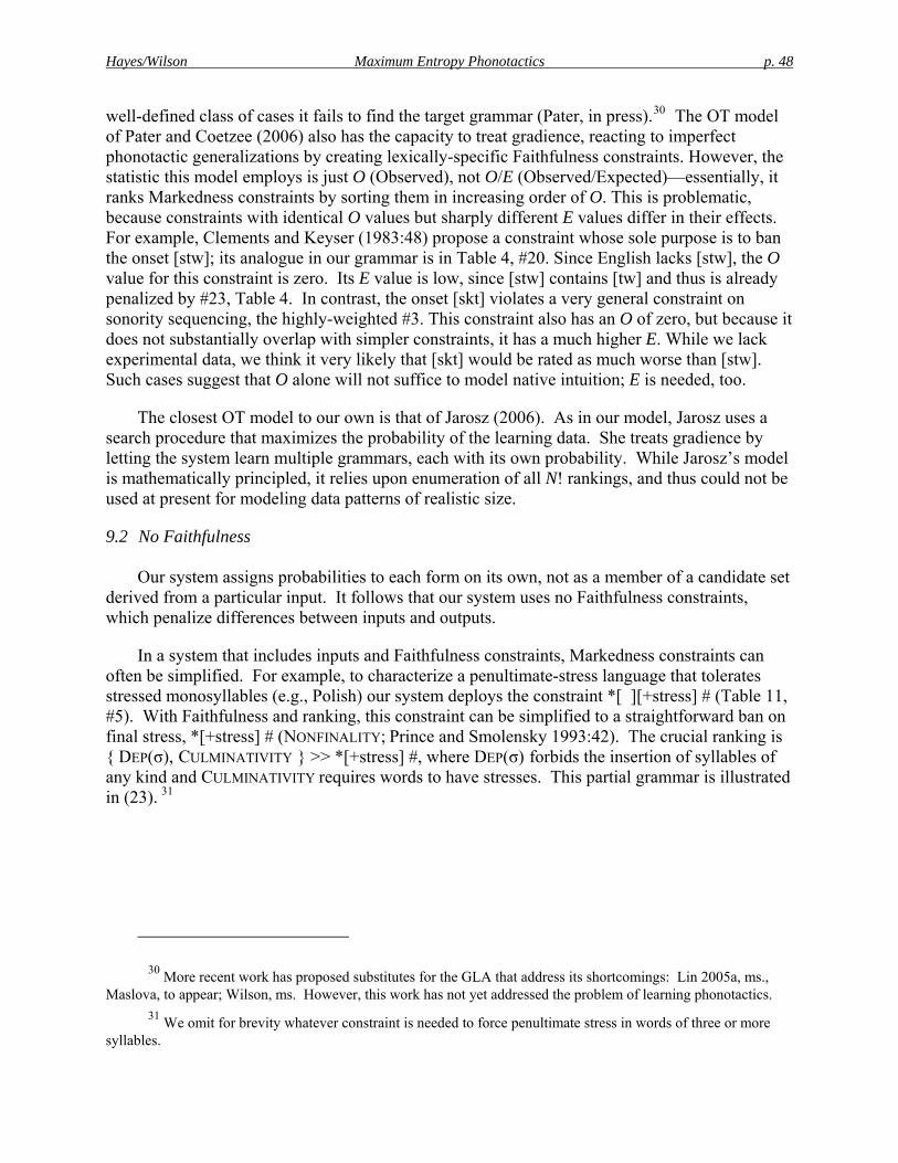
Hayes/Wilson Maximum Entropy Phonotactics p. 48
well-defined class of cases it fails to find the target grammar (Pater, in press).30 The OT model of Pater and Coetzee (2006) also has the capacity to treat gradience, reacting to imperfect phonotactic generalizations by creating lexically-specific Faithfulness constraints. However, the statistic this model employs is just O (Observed), not O/E (Observed/Expected)—essentially, it ranks Markedness constraints by sorting them in increasing order of O. This is problematic, because constraints with identical O values but sharply different E values differ in their effects. For example, Clements and Keyser (1983:48) propose a constraint whose sole purpose is to ban the onset [stw]; its analogue in our grammar is in Table 4, #20. Since English lacks [stw], the O value for this constraint is zero. Its E value is low, since [stw] contains [tw] and thus is already penalized by #23, Table 4. In contrast, the onset [skt] violates a very general constraint on sonority sequencing, the highly-weighted #3. This constraint also has an O of zero, but because it does not substantially overlap with simpler constraints, it has a much higher E. While we lack experimental data, we think it very likely that [skt] would be rated as much worse than [stw]. Such cases suggest that O alone will not suffice to model native intuition; E is needed, too.
The closest OT model to our own is that of Jarosz (2006). As in our model, Jarosz uses a search procedure that maximizes the probability of the learning data. She treats gradience by letting the system learn multiple grammars, each with its own probability. While Jarosz’s model is mathematically principled, it relies upon enumeration of all N! rankings, and thus could not be used at present for modeling data patterns of realistic size.
9.2 No Faithfulness
Our system assigns probabilities to each form on its own, not as a member of a candidate set derived from a particular input. It follows that our system uses no Faithfulness constraints, which penalize differences between inputs and outputs.
In a system that includes inputs and Faithfulness constraints, Markedness constraints can often be simplified. For example, to characterize a penultimate-stress language that tolerates stressed monosyllables (e.g., Polish) our system deploys the constraint *[ ][+stress] # (Table 11, #5). With Faithfulness and ranking, this constraint can be simplified to a straightforward ban on final stress, *[+stress] # (NONFINALITY; Prince and Smolensky 1993:42). The crucial ranking is DEP(σ), CULMINATIVITY >> *[+stress] #, where DEP(σ) forbids the insertion of syllables of any kind and CULMINATIVITY requires words to have stresses. This partial grammar is illustrated in (23). 31
30 More recent work has proposed substitutes for the GLA that address its shortcomings: Lin 2005a, ms., Maslova, to appear; Wilson, ms. However, this work has not yet addressed the problem of learning phonotactics.
31 We omit for brevity whatever constraint is needed to force penultimate stress in words of three or more syllables.
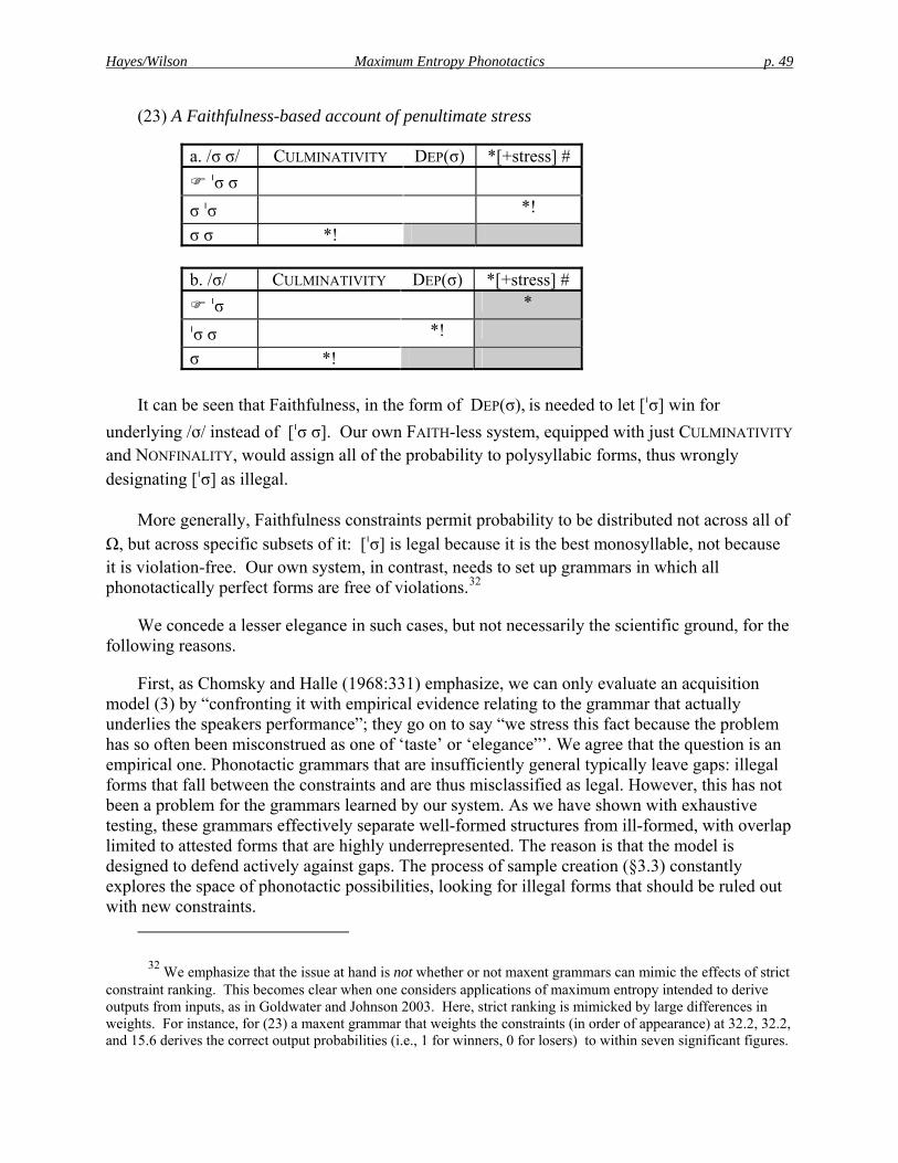
Hayes/Wilson Maximum Entropy Phonotactics p. 49
(23) A Faithfulness-based account of penultimate stress
a. /σ σ/ CULMINATIVITY DEP(σ) *[+stress] # ˈσ σ
σ ˈσ *! σ σ *!
b. /σ/ CULMINATIVITY DEP(σ) *[+stress] #
ˈσ *
ˈσ σ *! σ *!
It can be seen that Faithfulness, in the form of DEP(σ), is needed to let [ˈσ] win for
underlying /σ/ instead of [ˈσ σ]. Our own FAITH-less system, equipped with just CULMINATIVITY
and NONFINALITY, would assign all of the probability to polysyllabic forms, thus wrongly designating [ˈσ] as illegal.
More generally, Faithfulness constraints permit probability to be distributed not across all of Ω, but across specific subsets of it: [ˈσ] is legal because it is the best monosyllable, not because it is violation-free. Our own system, in contrast, needs to set up grammars in which all phonotactically perfect forms are free of violations.32
We concede a lesser elegance in such cases, but not necessarily the scientific ground, for the following reasons.
First, as Chomsky and Halle (1968:331) emphasize, we can only evaluate an acquisition model (3) by “confronting it with empirical evidence relating to the grammar that actually underlies the speakers performance”; they go on to say “we stress this fact because the problem has so often been misconstrued as one of ‘taste’ or ‘elegance”’. We agree that the question is an empirical one. Phonotactic grammars that are insufficiently general typically leave gaps: illegal forms that fall between the constraints and are thus misclassified as legal. However, this has not been a problem for the grammars learned by our system. As we have shown with exhaustive testing, these grammars effectively separate well-formed structures from ill-formed, with overlap limited to attested forms that are highly underrepresented. The reason is that the model is designed to defend actively against gaps. The process of sample creation (§3.3) constantly explores the space of phonotactic possibilities, looking for illegal forms that should be ruled out with new constraints.
32 We emphasize that the issue at hand is not whether or not maxent grammars can mimic the effects of strict constraint ranking. This becomes clear when one considers applications of maximum entropy intended to derive outputs from inputs, as in Goldwater and Johnson 2003. Here, strict ranking is mimicked by large differences in weights. For instance, for (23) a maxent grammar that weights the constraints (in order of appearance) at 32.2, 32.2, and 15.6 derives the correct output probabilities (i.e., 1 for winners, 0 for losers) to within seven significant figures.
Hayes/Wilson Maximum Entropy Phonotactics p. 50
The other reason to favor general grammars is that only such grammars can account for how humans extend their knowledge to new forms. For instance, a grammar of English that simply listed the existing syllable onsets would fail to generalize to unattested onsets in the way observed by Scholes (1966). Because our model seeks general constraints (§4.2.2) based on natural classes, it captures the distinctions among the unattested clusters tested by Scholes rather well. Whether the model would perform even more accurately if it made use of Faithfulness is a matter for future work to determine.
9.3 Relating phonotactics to alternation
Phonological alternation occurs when morphemes take on different forms in different contexts. It is related to phonotactics because alternations frequently are seen to enforce the phonotactics dynamically. For instance, the English plural morpheme /-z/ is altered to [-s] following voiceless obstruents, as in cups [kps], in order to avoid a violation of the phonotactic constraint that bans voicing disagreement in final obstruent clusters. This is the essence of the “conspiracy problem” (Kisseberth 1970), which has been the focus of a great deal of phonological theorizing, notably in Optimality Theory. OT seeks to reduce the description of alternations to the same principles that govern phonotactics: the ranking of Markedness over Faithfulness constraints results in both static restrictions on surface forms and alternations that respect those restrictions.
Despite the many successes achieved in OT, we are not convinced that the link between phonotactics and alternation is as tight as the theory claims. In fact, not all alternations solve phonotactic problems. In Yidiɲ phonology, [u] is chosen (productively) as the epenthetic vowel following a nasal consonant, yet there is no evident connection between nasality and [u] in Yidiɲ phonotactics (Hayes 1999b). English vowel length alternations (SPE) are phonotactically motivated insofar as they optimize foot structure (Prince 1990, Hayes 1995), but the accompanying quality alternations ([iː] ~ [ɛ], [eɪ] ~ [æ], [aɪ] ~ [ɪ], [oʊ] ~ []) have no evident phonotactic basis.
We suggest that the proper link between alternations and phonotactics is at the level of language learning: knowing the phonotactics makes it easier for the language learner to discover alternations. Thus, for example, an English-learning child who already knew the principle of voicing agreement in final obstruent clusters would be in a good position to understand and analyze the voicing alternation in the plural suffix (Albright and Hayes 2002, Hayes 2004, Prince and Tesar 2004). That is, it would be immediately apparent that the simple concatenation [kʌp]+[z] is insufficient for the plural of cup, owing to its phonotactic violation; and it would remain only to find the change needed to produce the correct output [kʌps].
There is experimental evidence compatible with this conception. Children evidently learn at least some of the phonotactics of their language very early (i.e., in infancy; see Hayes 2004 for literature review)—so that whatever model of acquisition is developed should in any event include the capacity to learn phonotactics solely from distributional data. Moreover, the experimental findings of Pater and Tessier (2003) suggest that phonotactic knowledge does indeed assist learners in finding alternation patterns. A learning system for phonological
Hayes/Wilson Maximum Entropy Phonotactics p. 51
alternations devised by Albright and Hayes (2002, 2003) already incorporates an elementary capacity to use phonotactic knowledge to assist learning, as does the OT-based system of Tesar and Prince (2003).
We suggest that human language learners first obtain an outline analysis of their language’s phonotactics, following the method described here, then take on the many forms of string mapping that must be learned: mapping from paradigmatic base forms to the other paradigm members (Albright 2002b), from bases to reduplicants (McCarthy and Prince 1995), from one free variant to another (Kawahara 2002), and so on. These mappings are learned as a maxent grammar that incorporates Faithfulness constraints. The constraints used for string mappings would include Markedness constraints learned at the phonotactic stage, but they might also include constraints learned from the mapping data themselves, to cover cases like the Yidiɲ and English alternations just mentioned.
This sketch is one instantiation of what we call learning-theoretic phonology, by which we mean a theory whose overall architecture recapitulates the incremental process through which phonological knowledge is acquired.
9.4 How is phonological typology to be explained?
While establishing the content of the acquisition module AM ((3) above) strikes us as the central theoretical challenge in phonology, there is a second question that also deserves attention: why are languages the way they are? More specifically, what is the basis for the systematic cross-linguistic patterns, especially involving markedness, that emerge from typological study? Certainly an inductive-baseline learner cannot explain them; typologically unnatural patterns that can be characterized by general and accurate constraints will be just as learnable as the typologically natural ones.
One possible response to this question would be to say that, as our inductive baseline strategy is pursued further, it will turn out that the only effective learning strategy is one with an extremely rich UG—a UG that incorporates the entire constraint set for phonology (Prince and Smolensky 1993/2004; Tesar and Smolensky 1998, 2000; McCarthy 2002). If so, the problem of typology will likely be solved, and the outcome of our efforts will be an inductive-baseline argument for the universal-constraint approach.
However, there are other ways to enrich the inductive baseline model that are more conservative in their reliance on UG. For instance, language learners could make use of their own phonetic experience, accessing it to discover phonetically natural constraints grounded in articulation and perception (Boersma 1998, Hayes 1999a, Steriade 1999, 2001a, b, Gordon 2004, Hayes, Kirchner and Steriade 2004). Preference for such constraints would constitute a learning bias in favor of phonological systems that are easier to produce or perceive, or that suffer a lesser recognition burden from alternation. For experimental evidence in favor of learning biases, and a mechanism (based on maximum entropy) whereby they could be incorporated into a general learning scheme, see Wilson (2006).
Further afield, we note that many scholars hold the view that not all typological patterns should be explained by UG; instead, the diachronic process of language transmission and
Hayes/Wilson Maximum Entropy Phonotactics p. 52
mistransmission is responsible for much or all of typology. For representative statements of this idea, see Ohala 1981, Baroni 2001, Blevins 2004, and Myers, ms.. We think that more serious assessment of this position will become possible as formally implemented models of the process of phonological evolution (de Boer 2001, Kochetov 2002, Boersma 2005, Boersma and Hamann 2006, Wedel 2007) become increasingly available and are applied to data patterns of realistic size.
9.5 Hidden structure
Tesar and Smolensky (1998, 2000) and Tesar (2004) address the problem of “hidden structure” in phonological learning. By this they mean structure that is not detectible in the phonetic signal, but which is phonologically present and provides order and systematicity to the data pattern. An example of hidden structure is syllable weight (e.g. Hayes 1995:§3.9.2): certain properties of syllables are used to classify them into light and heavy categories, which then can be used to make sense of other patterns, particularly stress.
Hidden structure is often partly language-specific; for example, different languages impose different criteria for what counts as a heavy syllable. This creates a “chicken-or-egg” problem: we need to know the language-specific criterion of syllable weight in order to detect the stress pattern, but it is often the stress pattern itself that gives the main evidence for the syllable weight criterion. Tesar and Smolensky offer intriguing methods, based on expectation maximization and inconsistency detection, to discover both the hidden structure and the generalizations based on it.
While our present model incorporates no clear cases of hidden structure, we believe it could be scaled up to learn it. The key idea is that the correct choice of hidden structure is detectable by maxent methods: the correct hidden structure will yield a tighter phonotactic characterization, which increases the probability of the learning data, a measurable quantity under the maxent approach. In future work we hope to address the problem in these terms.
9.6 Directions for future work
In expanding the approach taken here, we think an important line to follow will be to enrich the class of formal mechanisms it can access. In other words, while we have shown that vowel tiers and grids are important to phonotactic learning, we judge that our system is still too close to its original inductive baseline, as there are phonological phenomena it clearly cannot learn unless further modified. We end by giving two examples.
First, we cannot claim that our system of projections has fully solved the problem of learning nonlocal phonotactic dependencies. Notably, it cannot account for consonant-to-consonant dependencies of the kind studied in McCarthy 1979, 1988, MacEachern 1999, Frisch and Zawaydeh 2001, Frisch, Pierrehumbert, and Broe 2004, and Rose and Walker 2004. Simply adding a consonant projection is unlikely to suffice for these cases, because of two special factors. Consonant-to-consonant phonotactics relies heavily on similarity—those consonants that are most similar are the ones whose distribution is phonotactically regulated. Further, there are also gradient distance effects: consonants that are separated at a short distance are regulated more closely than those at greater distances. Neither of these effects could be modeled merely by introducing a consonant projection. We anticipate that the right approach would be to incorporate
Hayes/Wilson Maximum Entropy Phonotactics p. 53
a similarity metric into the theory (for a review of various possibilities, see Bailey and Hahn 2001) and use it to scan the nearby segments.
We also lack a theory to learn the phonotactics of neutral vowels; i.e. cases where particular vowels (not just consonants) are skipped over in vowel harmony. We are encouraged here by findings (Gordon 1999, Gick et al. 2006, Benus and Gafos 2007) that in their allophonic forms, neutral vowels can be weakly harmonic, taking on slightly different phonetic forms depending on the neighboring harmonic vowels. The incorporation of such phonetic detail into the representations would “localize” the phonotactics on the vowel projection, perhaps sufficing to make neutral-vowel phonotactics learnable.
Appendix A: Generating samples
As noted in §4.2.1, to obtain E[Ci] (expected violation counts) when we are seeking a new constraint to add to the grammar, we generate a “sample”; that is, a set of forms drawn from the probability distribution defined by the current grammar. Our procedure for sample creation is as follows. We assume that the current grammar has been represented as a finite state machine G, constructed as in §3.3.2. G is intersected with the machine that accepts Σ
n (the set of all strings
of length n), yielding an acyclic machine M, which represents every possible string x of length n together with its score h(x), as defined in (4).
Each transition t in M has a violation vector V(t), representing the violations incurred by any path traversing t. The cost of t is defined as e taken to the negative power of the dot product
of the current weights and V(t); i.e. exp(–Σi=1
N wi V(t)i). Following MacKay (2003), M is globally
normalized by dividing each transition t’s cost by the total cost of all paths from the terminus of t to the final state in M.
Samples of length n are generated by beginning at the initial state of M and randomly selecting transitions until the final state is reached. Specifically, if the current state is q, the probability of choosing transition t from q is equal to t’s share of the total probability of transitions leaving q. The number of samples of length n is determined by fitting a Poisson distribution to the observed distribution of lengths in the learning data, and the sample size as a whole roughly matches that of the learning data.
Appendix B: Modeling English onsets with “exotic” items included in the learning data
We mentioned in §5.1 that it hard to determine to what extent children pay attention to extremely rare onsets (e.g., from borrowed words) when learning English onset phonotactics. In the main text we report a simulation using only “nonexotic” data. In this appendix we show what happens when exotic onsets are included.
Following a method given in Pierrehumbert 2001b, we attempted to mimic the language learning experience of the children who participated in Scholes’s (1996) experiment. To this
Hayes/Wilson Maximum Entropy Phonotactics p. 54
end, we employed the CELEX English database (Baayen et al. 1995).33 We first removed the null-onset words, then obtained frequency estimates of the remaining 39,053 forms by counting the hits for each when searched on the Google search engine.34 We then used these counts as the basis of simulated childhoods: sampling from the overall token frequencies, we selected words to be included in the simulated vocabularies. A word was included in a vocabulary once it had been “heard” five times, and the vocabularies were set at 10,000 words. We repeated this procedure ten times.
This method yielded learning sets that included a modest number of exotic onsets, while matching closely in overall frequencies with the primary corpus (11), the median correlation being r = 0.967. We report here just one learning run, the one that did worst in matching the Scholes data. In this run, the training data included three “exotic” onsets (4 instances of [sr], 1 of [ʒ], and 1 of [sf]), but lacked any cases of [hw], [skl], or [θw]. Given these learning data, our model produced a grammar that correlated fairly well with the Scholes data (r = 0.929, compared to 0.946 for the main simulation given above), and did about as well as the main simulation in separating attested from unattested clusters. In the other nine learning sets, the correlation with the Scholes data ranged from 0.930 to 0.943.
We also tried simply learning a grammar from the type frequencies for all onsets, using the entire CELEX database. This produced a considerably larger number of “exotic” onsets (25 not included in (11)), and learning performance was somewhat worse. Correlation across ten runs with the Scholes data ranged from 0.913 to 0.928, and separation of legal forms from illegal was rather more haphazard.
We conclude that phonological learning is possible under our system with exotic onsets but that performance is better when the exotic forms are removed. It does not seem impossible that children could recognize exotic items as such, because they often contain clues to their status, specifically their limitation to learned words ([sf]), interjections ([pʃ]), or words describing faraway places and cultural items ([labial + w]).
Appendix C: Training sets and constraints for the stress typology of Gordon 2002
Constraints are listed in discovery order. Abbreviations: M = Main tier, S = Stress tier; otherwise Default tier; [s] = [stress], [m] = [main], 1 = [+main], 2 = [+stress, –main], 0 = [–stress].
33 We used CELEX here, not CMU, since we judged that the latter contains substantially more typographical errors. These are more perilous in preparing non-hand-edited corpora.
34 For discussion of this method, see Blair et al. 2002, Hayes and Londe 2006:64-65.
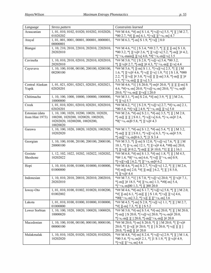
Hayes/Wilson Maximum Entropy Phonotactics p. 55
Language Stress pattern Constraints learned Araucanian 1, 01, 010, 0102, 01020, 010202, 0102020,
01020202 *## M 4.6, *#[-m] S 1.4, *[+s][+s] 5.5, *[ ][ ] M 2.7, *00 2.7, *#[ ][-m] 6.1, *[+s][ ][^+s,-m] 4.7
Atayal 1, 01, 001, 0001, 00001, 000001, 0000001, 00000001
*## M 6.3, *[-m] S 1.9, *[+s][ ] 8.0
Biangai 1, 10, 210, 2010, 22010, 202010, 2202010, 20202010
*## M 4.6, *1[ ] S 3.4, *#0 2.7, *[ ][ ][ ][-m] S 1.0, *00 3.2, *[ ][+s]# 2.6, *[ ][+s][+s] 5.2, *[-m][ ]# 4.2, *[^+s,-main][ ][+s] 4.0, *#[^+s,-m][+s] 3.5
Cavineña 1, 10, 010, 2010, 02010, 202010, 0202010, 20202010
*## M 5.0, *1[ ] S 2.8, *[+s][+s] 5.4, *00 3.2, *[ ][+s]# 2.7, *[-m][ ]# 4.3, *[^+s,-m][ ][+s] 4.4
Cayuvava 1, 10, 100, 0100, 00100, 200100, 0200100, 00200100
*## M 5.6, *[ ][-m] S 1.1, *[+s][+s] 2.5, *[ ][ ] M 1.6, *[ ][+s]# 4.6, *[+s][ ][+s] 1.9, *1[ ] S 1.8, *000 2.2, *[ ][+s][ ]# 3.0, *[+s][ ][ ][-m] 3.8, *[-m][ ][ ]# 3.5, *[^+s,-m][ ][ ][+s] 3.3
Central Alaskan Yupik
1, 01, 021, 0201, 02021, 020201, 0202021, 02020201
*## M 4.6, *1[ ] S 20.0, *[-m]# 20.0, *[ ][ ][ ][-m] S 4.6, *#[+s,-m] 20.0, *[+s][+s,-m] 20.0, *[^+s,-m]0 20.0, *[^+s,-m][ ][+s][ ] 20.0
Chitimacha 1, 10, 100, 1000, 10000, 100000, 1000000, 10000000
*## M 3.1, *[-m] S 2.6, *#[-m] 3.9, *[ ][ ] M 2.6, *[ ][+s] 5.7
Creek 1, 01, 010, 0201, 02010, 020201, 0202010, 02020201
*## M 6.2, *1[ ] S 2.9, *[+s][+s] 2.7, *#[+s,-m] 2.1, *00 5.4, *#[+s][ ] 4.9, *[^+s,-m][ ][+s] 5.0
Estonian (data from Hint 1973)
1, 10, 100, 1020, 10200, 10020, 102020, 100200, 1020200, 1020020, 1002020, 10202020, 10200200, 10020200, 10020020
*## M 2.6, *#[-m] S 2.1, *#[-m] 3.5, *[ ][ ] M 2.8, *[-m][ ][ ][ ] S 0.1, *[+s][+s] 6.6, *[+s,-m]# 2.4, *0[^+s,-m]0 5.8, *[ ][+s]# 4.3
Garawa 1, 10, 100, 1020, 10020, 102020, 1002020, 10202020
*## M 1.7, *#[-m] S 1.2, *#[-m] 5.4, *[ ][ ] M 3.2, *[-m][ ][ ][ ] S 0.1, *[+s][+s] 6.3, *[+s,-m]# 5.9, *[-m][^+s,-m]0 6.3, *[ ]1 S 3.4
Georgian 1, 10, 100, 0100, 20100, 200100, 2000100, 20000100
*## M 5.3, *[ ][-m] S 12.0, *[+s][+s] 7.6, *[ ][ ] M 10.1, *[ ][+s,-m] 12.1, *[ ][+s]# 4.4, *#0[-m] 20.0, *[ ][+s][ ]# 0.2, *[-m][ ][ ]# 10.0, *1[ ][ ][ ] 16.1
Gosiute Shoshone
1, 12, 102, 1022, 10202, 102022, 1020202, 10202022
*## M 6.8, *#[-m] S 1.3, *#[-m] 1.8, *[ ][ ] M 4.5, *0# 1.4, *0[^+s,-m] 6.6, *[+s][ ][^+s,-m] 0.9, *[+s][+s][ ] 6.2, *[ ][^+s,-m]# 6.2
Hopi 1, 10, 010, 0100, 01000, 010000, 0100000, 01000000
*## M 4.6, *[-m] S 2.7, *[+s][+s] 1.2, *[ ][ ] M 2.6, *#[-m][-m] 2.0, *#[ ][-m][ ] 6.2, *[ ][ ] S 5.0, *[ ][+s]# 4.4
Indonesian 1, 10, 010, 2010, 20010, 202010, 2002010, 20202010
*## M 7.5, *1[ ] S 7.0, *[+s][+s] 20.0, *[ ][+s]# 7.1, *[-m][ ]# 18.5, *#[ ][+s,-m] 1.3, *#0[-m] 5.4, *[^+s,-m]00 1.3, *[ ][ ]00 20.0
Ioway-Oto 1, 01, 010, 0100, 01002, 010020, 0100200, 01002002
*## M 4.6, *#[-m] S 1.7, *[+s][+s] 5.8, *[ ][ ] M 2.0, *#[ ][-m] 6.1, *[-m][ ][ ] S 1.0, *[+s][ ][+s] 4.6, *00[^+s,-m] 3.2, *[+s][ ][ ][^+s,-m] 3.6
Lakota 1, 01, 010, 0100, 01000, 010000, 0100000, 01000000
*## M 4.5, *[-m] S 2.8, *[+s][+s] 1.1, *[ ][ ] M 2.7, *#[ ][-m] 7.3, *[ ][ ] S 5.2
Lower Sorbian 1, 10, 100, 1020, 10020, 100020, 1000020, 10000020
*## M 5.0, *#[-m] S 5.4, *#[-m] 20.0, *[ ][ ] M 20.0, *[-m][ ] S 20.0, *[+s][+s] 20.0, *[+s,-m]# 20.0, *[+s,-m][ ][ ] 20.0, *[-m][^+s,-m][ ]# 20.0
Macedonian 1, 10, 100, 0100, 00100, 000100, 0000100, 00000100
*## M 20.0, *[-m] S 20.0, *[ ][ ] M 20.0, *[ ][+s]# 20.0, *[ ][+s][ ]# 20.0, *[ ][ ] S 20.0, *[+s][ ][ ][ ] 20.0, *[-m][ ][ ]# 20.0
Malakmalak 1, 10, 010, 1020, 01020, 102020, 0102020, 10202020
*## M 4.8, *#[-m] S 2.4, *[+s][+s] 2.9, *[ ][ ] M 1.4, *00 5.4, *[+s,-m]# 2.1, *[ ]1 S 1.9, *[ ][+s]# 4.9, *[+s][ ][^+s,-m] 4.6

Hayes/Wilson Maximum Entropy Phonotactics p. 56
Maranungku 1, 10, 102, 1020, 10202, 102020, 1020202, 10202020
*## M 20.0, *#[-m] S 11.5, *#[-m] 11.5, *[ ][ ] M 4.0, *[-m][ ][ ][ ] S 5.4, *[+s][+s] 20.0, *0[^+s,-m] 20.0, *[+s][ ][ ][+s] 2.8
Nahuatl 1, 10, 010, 0010, 00010, 000010, 0000010, 00000010
*## M 4.6, *[-m] S 2.9, *[+s][+s] 1.8, *[ ][ ] M 2.9, *[ ][+s]# 3.5, *[+s][ ][ ] 5.1, *[-m][ ]# 3.8
Pacific Yupik 1, 01, 010, 0102, 01002, 010020, 0100202, 01002002
*## M 4.6, *#[-m] S 1.4, *[+s][+s] 5.9, *[ ][ ] M 2.5, *#[ ][-m] 6.2, *[-m][ ][ ] S 1.1, *00# 2.2, *00[^+s,-m] 1.8, *[+s][ ][ ][^+s,-m] 5.9, *[+s][ ][^+s,-m]# 3.7
Palestinian Arabic
1, 10, 201, 2010, 20201, 202010, 2020201, 20202010
*## M 6.2, *1[ ] S 7.1, *[+s][+s] 6.8, *#0 6.1, *00 6.5
Pintupi 1, 10, 100, 1020, 10200, 102020, 1020200, 10202020
*## M 2.8, *#[-m] S 1.8, *#[-m] 3.5, *[ ][ ] M 2.7, *[-m][ ][ ][ ] S 0.2, *[+s][+s] 6.1, *[+s,-m]# 5.3, *0[ ][+s] 2.0, *0[^+s,-m][ ] 5.6, *[ ]1 3.4
Piro 1, 10, 010, 2010, 20010, 202010, 2020010, 20202010
*## M 5.1, *1[ ] S 5.8, *[+s][+s] 5.6, *[ ][+s]# 3.0, *[-m][ ]# 3.7, *#[ ][+s,-m] 2.2, *#0[-m] 4.7, *[^+s,-m][ ][+s,-m] 1.5, *[^+s,-m]0[-m] 5.2
Quebec French 1, 21, 201, 2001, 20001, 200001, 2000001, 20000001
*## M 2.7, *[ ][-m] S 3.9, *[-m]# 4.4, *[ ][ ] M 2.6, *#0 7.3, *[ ][ ][ ] S 3.8, *1[ ] 4.3
Sanuma 1, 10, 010, 2010, 20010, 200010, 2000010, 20000010
*## M 5.0, *[ ][-m] S 3.1, *[+s][+s] 4.5, *[ ][ ] M 3.1, *[ ][+s,-m] 3.5, *[ ][+s]# 2.7, *[-m][ ]# 4.2, *#0[-m] 5.8, *1[ ][ ] 4.4
Southern Paiute 1, 10, 010, 0120, 01020, 010220, 0102020, 01020220
*## M 4.6, *#[-m] S 1.4, *[+s]1 2.2, *[ ][ ] M 2.0, *[-m][ ][ ][ ] S 0.1, *00 5.4, *[+s,-m]# 2.2, *#[+s][+s] 1.0, *[ ]1 S 2.4, *[+s][+s][+s] 5.0, *#[ ][-m][ ] 5.8, *[+s][ ][^+s,-m][ ] 5.6, *[ ][+s]# 4.9
Tauya 1, 21, 201, 2201, 20201, 220201, 2020201, 22020201
*## M 3.5, *1[ ] S 5.6, *[-m]# 3.8, *#0 5.6, *[^+s,-m]0 6.3, *[ ][+s][+s] 6.5
Udihe 1, 01, 201, 2001, 20001, 200001, 2000001, 20000001
*## M 2.9, *[ ][-m] S 3.3, *[+s][+s] 4.4, *[ ][ ] M 3.1, *[-m]# 4.2, *[ ][+s,-m] 3.7, *#[^+s,-m][-m] 6.0, *1[ ] 4.4
Urubu Kapor 1, 01, 201, 0201, 20201, 020201, 2020201, 02020201
*## M 3.6, *1[ ] S 1.9, *[+s][+s] 6.9, *[-m]# 3.8, *[^+s,-m]0 6.7
Walmatjari (data from Hudson 1978)
1, 10, 100, 1020, 10200, 10020, 100200, 100020, 1000200, 1000020, 10000200, 10000020
*## M 20.0, *#[-m] S 20.0, *#[-m] 20.0, *[ ][ ] M 5.1, *[-m][ ] S 20.0, *[+s][+s] 20.0, *[+s,-m]# 20.0, *0[^+s,-m][ ]# 20.0
Winnebago 1, 01, 001, 0010, 00102, 001002, 0010020, 00100202
*## M 4.7, *#[-m] S 1.5, *[+s][+s] 20.0, *[ ][ ] M 14.6, *#[+s][ ] 4.4, *[-m]00 20.0, *[ ]1 S 14.6, *00# 20.0, *[-m][ ][ ] S 20.0, *#[ ][ ][-m] 20.0, *[+s][ ][ ][^+s,-m] 14.5
Appendix D: Constraints for Wargamay not discussed in the text
All constraints listed were discovered on the default projection.
Constraint Weight
1. *[+syl][+son,+dors][–back] 3.91 2. *[+long][+ant,–lat][^–long,–high,–str] 3.65 3. *[+son,–approx][^–long,+back,–str]# 3.60 4. *[–approx][–syl][^–long] 3.55 5. *[+high,–main,+str][–lat] 3.51 6. *[–main][–son,+ant][+high,–main] 3.49
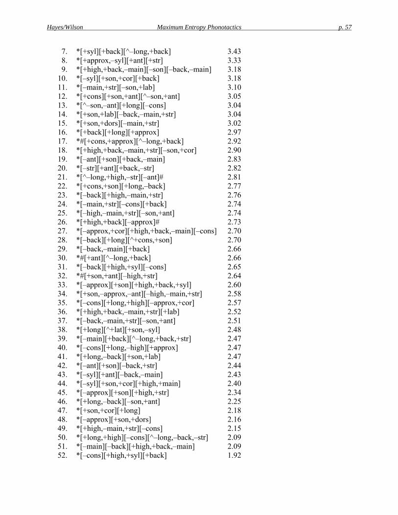
Hayes/Wilson Maximum Entropy Phonotactics p. 57
7. *[+syl][+back][^–long,+back] 3.43 8. *[+approx,–syl][+ant][+str] 3.33 9. *[+high,+back,–main][–son][–back,–main] 3.18 10. *[–syl][+son,+cor][+back] 3.18 11. *[–main,+str][–son,+lab] 3.10 12. *[+cons][+son,+ant][^–son,+ant] 3.05 13. *[^–son,–ant][+long][–cons] 3.04 14. *[+son,+lab][–back,–main,+str] 3.04 15. *[+son,+dors][–main,+str] 3.02 16. *[+back][+long][+approx] 2.97 17. *#[+cons,+approx][^–long,+back] 2.92 18. *[+high,+back,–main,+str][–son,+cor] 2.90 19. *[–ant][+son][+back,–main] 2.83 20. *[–str][+ant][+back,–str] 2.82 21. *[^–long,+high,–str][–ant]# 2.81 22. *[+cons,+son][+long,–back] 2.77 23. *[–back][+high,–main,+str] 2.76 24. *[–main,+str][–cons][+back] 2.74 25. *[–high,–main,+str][–son,+ant] 2.74 26. *[+high,+back][–approx]# 2.73 27. *[–approx,+cor][+high,+back,–main][–cons] 2.70 28. *[–back][+long][^+cons,+son] 2.70 29. *[–back,–main][+back] 2.66 30. *#[+ant][^–long,+back] 2.66 31. *[–back][+high,+syl][–cons] 2.65 32. *#[+son,+ant][–high,+str] 2.64 33. *[–approx][+son][+high,+back,+syl] 2.60 34. *[+son,–approx,–ant][–high,–main,+str] 2.58 35. *[–cons][+long,+high][–approx,+cor] 2.57 36. *[+high,+back,–main,+str][+lab] 2.52 37. *[–back,–main,+str][–son,+ant] 2.51 38. *[+long][^+lat][+son,–syl] 2.48 39. *[–main][+back][^–long,+back,+str] 2.47 40. *[–cons][+long,–high][+approx] 2.47 41. *[+long,–back][+son,+lab] 2.47 42. *[–ant][+son][–back,+str] 2.44 43. *[–syl][+ant][–back,–main] 2.43 44. *[–syl][+son,+cor][+high,+main] 2.40 45. *[–approx][+son][+high,+str] 2.34 46. *[+long,–back][–son,+ant] 2.25 47. *[+son,+cor][+long] 2.18 48. *[–approx][+son,+dors] 2.16 49. *[+high,–main,+str][–cons] 2.15 50. *[+long,+high][–cons][^–long,–back,–str] 2.09 51. *[–main][–back][+high,+back,–main] 2.09 52. *[–cons][+high,+syl][+back] 1.92
Hayes/Wilson Maximum Entropy Phonotactics p. 58
53. *[+back,–syl][–syl] 1.84 54. *[+long][+back] 1.52 55. *[–syl][+son,+cor][+high,+back] 1.16 56. *[–syl][+ant][–ant] 0.95 57. *[+son,+cor][+long,–back] 0.40
References
Albright, Adam. 2002a. Islands of reliability for regular morphology: Evidence from Italian. Language 78:684-709.
Albright, Adam. 2002b. The identification of bases in morphological paradigms. Doctoral dissertation, University of California, Los Angeles.
Albright, Adam. 2006. Gradient phonotactic effects: lexical? grammatical? both? neither? Talk presented at the 80th Annual Meeting of the Linguistic Society of America, Albuquerque.
Albright, Adam, and Bruce Hayes. 2002. Modeling English past tense intuitions with minimal generalization. In Proceedings of the 2002 Workshop on Morphological Learning, Association of Computational Linguistics, ed. Michael Maxwell, 58-69. Philadelphia: Association for Computational Linguistics.
Albright, Adam, and Bruce Hayes. 2003. Rules vs. analogy in English past tenses: a computational/experimental study. Cognition 90:119–161.
Albro, Daniel M. 1998. Evaluation, implementation, and extension of Primitive Optimality Theory. Master’s thesis, University of California, Los Angeles.
Albro, Daniel M. 2005. Computational Optimality Theory and the phonological system of Malagasy. Doctoral dissertation, University of California, Los Angeles.
Allauzen, Cyril, Mehryar Mohri, and Brian Roark. 2005. The design principles and algorithms of a weighted grammar library. International Journal of Foundations of Computer Science 16:403– 421.
Archangeli, Diana. 1984. Underspecification in Yawelmani phonology and morphology. New York: Garland.
Archangeli, Diana, and Douglas Pulleyblank. 1987. Maximal and minimal rules: effects of tier scansion. In Proceedings of the North Eastern Linguistic Society 17, ed. Joyce McDonough and Bernadette Plunkett, 16–35. Amherst: Graduate Linguistics Student Association, University of Massachusetts.
Baayen, R. Harald, Piepenbrock, R., & Gulikers, L. 1995. The CELEX Lexical Database (Release 2) [CD-ROM]. Philadelphia, Penn.: Linguistic Data Consortium, University of Pennsylvania [Distributor].
Bailey, Todd M., and Ulrike Hahn. 2001. Determinants of wordlikeness: Phonotactics or lexical neighborhoods. Journal of Memory and Language 44:568–591.
Baker, C. L. 1979. Syntactic theory and the projection problem. Linguistic Inquiry 10:533-581. Baroni, Marco. 2001. How do languages get crazy constraints? Phonetically-based phonology
and the evolution of the Galeata Romagnolo vowel system. UCLA Working Papers in Linguistics 7, ed. Adam Albright and Taehong Cho, 152-178.
Beckman, Jill. 1997. Positional faithfulness, positional neutralisation and Shona vowel harmony. Phonology 14:1–46.
Benus, Stefan, and Adamantios Gafos. 2007. Articulatory characteristics of Hungarian ‘transparent’ vowels. Journal of Phonetics 35:271–300.
Hayes/Wilson Maximum Entropy Phonotactics p. 59
Berent, Iris, Donca Steriade, Tracy Lennertz, and Vered Vaknin. 2007. What we know about what we have never heard: Evidence from perceptual illusions. Cognition 104:591–630.
Berger, Adam L. No date. Convexity, maximum likelihood and all that. Ms., Department of Computer Science, Carnegie Mellon University. http://www.cs.cmu.edu/afs/cs/user/aberger/www/ ps/convex.ps
Berger, Adam L., Stephen A. Della Pietra, and Vincent J. Della Pietra. 1996. A maximum entropy approach to natural language processing. Computational Linguistics 22:39–71.
Blair, Irene V., Geoffrey R. Urland, and Jennifer E. Ma. 2002. Using Internet search engines to estimate word frequency. Behavior Research Methods, Instruments, & Computers 34: 286-290.
Blevins, Juliette. 2004. Evolutionary phonology: The emergence of sound patterns. Cambridge: Cambridge University Press.
Bloomfield, Leonard. 1933. Language. New York: Henry Holt. Boersma, Paul. 1997. How we learn variation, optionality, and probability. In Institute of
Phonetic Sciences, University of Amsterdam, Proceedings 21, 43–58. Boersma, Paul. 1998. Functional Phonology: Formalizing the interactions between articulatory
and perceptual drives. Doctoral dissertation, University of Amsterdam. The Hague: Holland Academic Graphics.
Boersma, Paul. 2004. A Stochastic OT account of paralinguistic tasks such as grammaticality and prototypicality judgments. Rutgers Optimality Archive 648.
Boersma, Paul. 2005. Prototypicality judgments as inverted perception. Rutgers Optimality Archive 742.
Boersma, Paul, Paola Escudero and Rachel Hayes. 2003. Learning abstract phonological from auditory phonetic categories: An integrated model for the acquisition of language-specific sound categories. In Proceedings of the 15th International Congress of Phonetic Sciences, Barcelona, ed. M. J. Sole, D. Recasens and J. Romero, 1013-1016.
Boersma, Paul, and Silke Hamann. 2006. Sibilant inventories in bidirectional phonology and phonetics. Talk presented at OCP 3, Budapest, January 17, 2006.
Boersma, Paul, and Bruce Hayes. 2001. Empirical tests of the Gradual Learning Algorithm. Linguistic Inquiry 32:45–86.
Bybee, Joan. 1995. Regular morphology and the lexicon. Language and Cognitive Processes 10:425–455.
Bybee, Joan. 2001. Phonology and language use. Cambridge: Cambridge University Press. Chomsky, Noam. 1963. Formal properties of grammars. In Handbook of Mathematical
Psychology, ed. R. D. Luce, R. R. Bush, and E. Galanter, volume II, 323–418. New York: Wiley.
Chomsky, Noam, and Morris Halle. 1965. Some controversial questions in phonological theory. Journal of Linguistics 1:97–138.
Chomsky, Noam, and Morris Halle. 1968. The sound pattern of English. New York: Harper and Row.
Clements, George N. 1976. Neutral vowels in Hungarian vowel harmony: an autosegmental interpretation. In Proceedings of the Seventh Annual Meeting of North Eastern Linguistic Society, ed. Judy Kegl, David Nash, and Annie Zaenen, 49–64.
Clements, George N., and Elizabeth V. Hume. 1995. The internal organization of speech sounds. In The handbook of phonological theory, ed. John Goldsmith, 245–306. Oxford: Blackwell.
Hayes/Wilson Maximum Entropy Phonotactics p. 60
Clements, George N., and S. Jay Keyser. 1983. CV Phonology: A Generative Theory of the Syllable. Cambridge, Mass.: MIT Press.
Clements, George N., and Engin Sezer. 1982. Vowel and consonant disharmony in Turkish. In The Structure of Phonological Representations (part II), ed. Harry van der Hulst and Norval Smith, 213–256. Dordrecht: Foris.
Coleman, John, and Janet Pierrehumbert. 1997. Stochastic phonological grammars and acceptability. In Computational Phonology, Third Meeting of the ACL Special Interest Group in Computational Phonology, 49–56. Somerset, N.J.: Association for Computational Linguistics.
Coetzee, Andries. 2004. What it means to be a loser: non-optimal candidates in Optimality Theory. Doctoral dissertation, University of Massachusetts, Amherst. Rutgers Optimality Archive 874.
Cover, Thomas M. and Joy A. Thomas. 1991. Elements of information theory. Hoboken, N.J.: Wiley.
de Boer, Bart. 2001. The Origins of vowel systems. Oxford: Oxford University Press. Davidson, Lisa. 2006. Phonology, phonetics, or frequency: Influences on the production of non-
native sequences. Journal of Phonetics 34:104–137. Della Pietra, Stephen, Vincent J. Della Pietra, and John D. Lafferty. 1997. Inducing features of
random fields. IEEE Transactions on Pattern Analysis and Machine Intelligence 19:380–393.
De Lacy, Paul. 2004. Markedness conflation in Optimality Theory. Phonology 21:145-199. Dixon, Robert M. W. 1981. Wargamay. In Handbook of Australian languages, volume II, ed.
Robert M. W. Dixon and Barry J. Blake, 1–144. Amsterdam: John Benjamins. Dresher, B. Elan, and Jonathan Kaye. 1990. A computational learning model for metrical
phonology. Cognition 20:421–451. Duda, Richard O., Peter E. Hart, and David G. Stork. 2001. Pattern classification, 2nd ed. New
York: Wiley. Eisner, Jason. 1997. Efficient generation in primitive Optimality Theory. In Proceedings of the
35th Annual Meeting of the Association for Computational Linguistics, 313–320. East Stroudsburg, Penn.: Association for Computational Linguistics.
Eisner, Jason. 2001. Expectational semirings: Flexible EM for finitestate transducers. In Proceedings of the ESSLLI Workshop on Finite-State Methods in NLP (FSMNLP), ed. G. van Noord.
Eisner, Jason. 2002. Parameter estimation for probabilistic finite-state transducers. In Proceedings of the 40th Annual Meeting of the Association for Computational Linguistics, 1–8. East Stroudsburg, Penn.: Association for Computational Linguistics.
Ellison, T. Mark. 1994. Phonological derivation in Optimality Theory. In Proceedings of the Fifteenth International Conference on Computational Linguistics, 1007–1013.
Fortune, G. 1955. An analytical grammar of Shona. London: Longmans, Green & Co. Frisch, Stefan A., Nathan R. Large, and David B. Pisoni. 2000. Perception of wordlikeness:
Effects of segment probability and length on the processing of nonwords. Journal of Memory and Language 42:481–496.
Frisch, Stefan A., Janet B. Pierrehumbert, and Michael Broe. 2004. Similarity avoidance and the OCP. Natural Language and Linguistic Theory 22:179–228.
Frisch, Stefan A., and Bushra A. Zawaydeh. 2001. The psychological reality of OCP-place in Arabic. Language 77:91–106.
Hayes/Wilson Maximum Entropy Phonotactics p. 61
Fudge, Erik C. 1969. Syllables. Journal of Linguistics 5:253–287. Fudge, Erik C. and Linda Shockey. No date. The Reading Syllable Database.
http://www.rdg.ac.uk/app_ling/sylls.htm. Gick, Bryan, Douglas Pulleyblank, Fiona Campbell, and Ngessimo Mutaka. 2006. Low vowels
and transparency in Kinande vowel harmony. Phonology 23: 1–20. Gildea, Daniel, and Daniel Jurafsky. 1996. Learning bias and phonological rule induction.
Computational Linguistics 22:497–530. Goldsmith, John. 1979. Autosegmental phonology. New York: Garland. Goldsmith, John, and Aris Xanthos. 2006. Learning phonological categories. Ms., Department
of Linguistics, University of Chicago. Downloaded May 21, 2007 from http://hum.uchicago.edu/~jagoldsm/Papers/phonolcat.pdf.
Goldwater, Sharon. 2007. Nonparametric Bayesian models of lexical acquisition. Doctoral dissertation, Brown University.
Goldwater, Sharon, and Mark Johnson. 2003. Learning OT constraint rankings using a maximum entropy model. In Proceedings of the Stockholm Workshop on Variation within Optimality Theory, ed. Jennifer Spenader, Anders Eriksson, and Osten Dahl, 111–120.
Gordon, Matthew. 1999. The “neutral” vowels of Finnish: How neutral are they? Linguistica Uralica 35:17–21.
Gordon, Matthew. 2002. A factorial typology of quantity insensitive stress. Natural Language and Linguistic Theory 20:491-552.
Gordon, Matthew. 2004. Syllable weight. In Phonetically based phonology, ed. Bruce Hayes, Robert Kirchner, and Donca Steriade, 277–312. Cambridge: Cambridge University Press.
Greenberg, Joseph H. 1978. Some generalizations concerning initial and final consonant clusters. In Universals of human language, vol. 2: phonology, ed. Joseph Greenberg, Charles Ferguson, and Edith Moravcsik, 243-280. Stanford: Stanford University Press.
Greenberg, Joseph H., and J. J. Jenkins. 1964. Studies in the psychological correlates of the sound system of American English. Word 20:157–177.
Grünwald, Peter, In Jae Myung, and Mark Pitt, ed. 2005. Advances in minimum description length: theory and applications. Cambridge, Mass.: MIT Press.
Hale, John, and Paul Smolensky. 2006. Harmonic Grammars and harmonic parsers for formal languages. In Smolensky and Legendre 2006, 393-416.
Halle, Morris. 1959. The sound pattern of Russian. The Hague: Mouton. Halle, Morris, and George N. Clements. 1983. Problem book in phonology. Cambridge, Mass.:
MIT Press. Halle, Morris, and Jean-Roger Vergnaud. 1987. An essay on stress. Cambridge, Mass.: MIT
Press. Hammond, Michael. 1999. The phonology of English: a prosodic Optimality-theoretic approach.
Oxford: Oxford University Press. Hammond, Michael. 2004. Gradience, phonotactics, and the lexicon in English phonology.
International Journal of English Studies 4:1-24. Hannan, M. 1959. Standard Shona dictionary. New York: St Martin’s Press. Hannan, M. 1981. Standard Shona dictionary, 2nd edition with addendum. Salisbury, Harare:
The Literature Bureau. Hay, Jennifer, Janet B. Pierrehumbert, and Mary Beckman. 2003. Speech perception, well-
formedness, and the statistics of the lexicon. In Papers in laboratory phonology VI, ed. John
Hayes/Wilson Maximum Entropy Phonotactics p. 62
Local, Richard Ogden, and Rosalind Temple, 58–74. Cambridge: Cambridge University Press.
Hayes, Bruce. 1995. Metrical stress theory: principles and case studies. Chicago: University of Chicago Press.
Hayes, Bruce. 1999a. Phonetically-driven phonology: the role of Optimality Theory and inductive grounding. In Functionalism and formalism in linguistics, volume I: general papers, ed. Mike Darnell, Edith Moravcsik, Michael Noonan, Frederick Newmeyer, and Kathleen Wheatley, 243– 285. Amsterdam: John Benjamins.
Hayes, Bruce. 1999b. Phonological restructuring in Yidiɲ and its theoretical consequences. In The derivational residue in phonological Optimality Theory, ed. Ben Hermans and Marc Oostendorp, 175–295. Amsterdam: John Benjamin.
Hayes, Bruce. 2000. Gradient well-formedness in Optimality Theory. In Optimality Theory: phonology, syntax, and acquisition, ed. Joost Dekkers, Frank van der Leeuw and Jeroen van de Weijer, 88-120. Oxford: Oxford University Press.
Hayes, Bruce. 2004. Phonological acquisition in Optimality Theory: the early stages. In Fixing priorities: constraints in phonological acquisition, ed. René Kager, Joe Pater, and Wim Zonneveld, 158-203. Cambridge: Cambridge University Press.
Hayes, Bruce, Robert Kirchner, and Donca Steriade, eds. 2004. Phonetically-based phonology. Cambridge: Cambridge University Press.
Hayes, Bruce, and Zsuzsa Cziráky Londe. 2006. Stochastic phonological knowledge: the case of Hungarian vowel harmony. Phonology 23:59–104.
Heinz, Jeffrey. to appear-a. Learning phonotactic patterns from surface forms. In Proceedings of the 25th West Coast Conference on Formal Linguistics, ed. Donald Baumer, David Montero, and Michael Scanlon. Somerville, Mass.: Cascadilla Proceedings Project.
Heinz, Jeffrey. to appear-b. Learning quantity-insensitive stress patterns via local inference. In Proceedings of The Association for Computational Linguistics Special Interest Group in Phonology 6 (ACL-SIGPHON 06). East Stroudsburg, Penn.: Association for Computational Linguistics.
Hint, Mati. 1973. Eesti keele sonafonoloogia I. Tallinn, Estonia: Eesti NSV Teaduste Akadeemia.
Hopcroft, John E., and Jeffrey D. Ullman. 1979. Introduction to automata theory, languages, and computation. Reading, Mass.: Addison-Wesley.
Hudson, Joyce. 1978. The core of Walmatjari grammar. Canberra: Australian Institute of Aboriginal Studies.
Jäger, Gerhard. 2004. Maximum entropy models and stochastic Optimality Theory. Rutgers Optimality Archive 625.
Jäger, Gerhard, and Anette Rosenbach. 2006. The winner takes it all – almost. Linguistics 44:937–971.
Jarosz, Gaja. 2006. Rich lexicons and restrictive grammars – maximum likelihood learning in Optimality Theory. Doctoral dissertation, Johns Hopkins University, Baltimore, Md.
Jaynes, Edwin T. 1983. Papers on probability, statistics, and statistical physics, ed. R. D. Rosenkrantz. Dordrecht: D. Reidel.
Jelinek, Frederick. 1999. Statistical methods for speech recognition. Cambridge, Mass.: MIT Press.
Hayes/Wilson Maximum Entropy Phonotactics p. 63
Jurafsky, Daniel, and James H. Martin. 2000. Speech and language processing: an introduction to natural language processing, computational linguistics, and speech recognition. Upper Saddle River, N.J.: Prentice Hall.
Kager, René. 1995. The metrical theory of word stress. In The handbook of phonological theory, ed. John Goldsmith, 367–402. Oxford: Blackwell.
Kawahara, Shigeto. 2002. Similarity among Variants: Output-Variant Correspondence. Bachelor’s thesis, International Christian University.
Keller, Frank. 2000. Gradience in grammar: experimental and computational aspects of degrees of grammaticality. Doctoral dissertation, University of Edinburgh.
Keller, Frank. 2006. Linear Optimality Theory as a model of gradience in grammar. In Gradience in grammar: generative perspectives, ed. Gisbert Fanselow, Caroline Fery, Ralph Vogel, and Matthias Schlesewsky, 270-287. Oxford University Press.
Kelly, Michael H. 1991. Using sound to solve syntactic problems: the role of phonology in grammatical category assignments. Psychological Review 99:349–364.
Kiparsky, Paul. 1973. Phonological representations. In Three dimensions of linguistic theory, ed. Osamu Fujimura. Tokyo: TEC.
Kiparsky, Paul. 1982. Lexical Phonology and Morphology. In Linguistics in the morning calm, ed. In-Seok Yang, 3–91. Seoul: Hanshin.
Kisseberth, Charles W. 1970. On the functional unity of phonological rules. Linguistic Inquiry 1:291–306.
Klein, Dan, and Christopher Manning. 2003. Maxent models, conditional estimation, and optimization, without the magic. Tutorial presented at NAACL-03 and ACL-03.
Kochetov, Alexei. 2002. Production, perception, and emergent phonotactic patterns. New York: Routledge.
Leben, William. 1973. Suprasegmental phonology. Doctoral dissertation, MIT, Cambridge, Mass.
Legendre, Géraldine, Yoshiro Miyata, and Paul Smolensky. 1990. Harmonic grammar: A formal multi-level connectionist theory of linguistic well-formedness: an application. In COGSCI 1990, 884–891.
Legendre, Géraldine, Antonella Sorace, and Paul Smolensky. 2006. The Optimality Theory - Harmonic Grammar connection. In Smolensky and Legendre 2006, 339–402.
Liberman, Mark. 1975. The intonational system of English. Doctoral dissertation, MIT, Cambridge, Mass.
Liberman, Mark, and Alan Prince. 1977. On stress and linguistic rhythm. Linguistic Inquiry 8:249–336.
Lin, Ying. 2005a. Learning Stochastic OT Grammars: A Bayesian approach using Data Augmentation and Gibbs Sampling. Proceedings of the Association for Computational Linguistics. East Stroudsburg, Penn.: Association for Computational Linguistics.
Lin, Ying. 2005b. Learning features and segments from waveforms: a statistical model of early phonological acquisition. Doctoral dissertation, University of California, Los Angeles.
Lin, Ying. Ms. Stochastic Optimality Theory, local search, and Bayesian learning of hierarchical linguistic models. Ms., Department of Linguistics, University of Arizona. Downloaded from http://dingo.sbs.arizona.edu/%7Eyinglin/Lin_hierarchical.pdf
MacEachern, Margaret R. 1999. Laryngeal cooccurrence restrictions. New York: Garland. MacKay, David J. C. 2003. Information theory, inference, and learning algorithms. Cambridge:
Cambridge University Press.
Hayes/Wilson Maximum Entropy Phonotactics p. 64
McCarthy, John. 1979. Formal problems in Semitic phonology and morphology. Doctoral dissertation, MIT, Cambridge.
McCarthy, John. 1986. OCP effects: gemination and antigemination. Linguistic Inquiry 17:207-263.
McCarthy, John. 1988. Feature geometry and dependency: a review. Phonetica 45:84–108. McCarthy, John. 2002. A thematic guide to Optimality Theory. Cambridge: Cambridge
University Press. McCarthy, John, and Alan Prince. 1995. Faithfulness and reduplicative identity. Papers in
Optimality Theory, University of Massachusetts Occasional Papers 18, ed. Jill Beckman, Laura Walsh Dickey and Suzanne Urbanczyk, 249-384. Amherst, Mass.: Graduate Linguistic Student Association.
McGarrity, Laura W. 2002. On the typological predictions of fixed vs. complementary rankings of stress constraints. In Online Proceedings of the 2002 Texas Linguistics Society, ed. A. Aguwele and H. Park. University of Texas, Austin: Texas Linguistic Forum.
Malouf, Robert. 2002. A comparison of algorithms for maximum entropy parameter estimation. In Proceedings of the Sixth Conference on Natural Language Learning (CoNLL-2002), 49-55.
Manning, Chris, and Hinrich Schütze. 1999. Foundations of statistical natural language processing. Cambridge, Mass.: MIT Press.
Maslova, Elena. To appear. Stochastic OT as a model of constraint interaction. To appear in Jane Grimshaw, Joan Maling, Chris Manning, Jane Simpson, and Annie Zaenen (eds.), Architectures, Rules, and Preferences: A Festschrift for Joan Bresnan. CSLI publications.
Mielke, Jeff. 2004. The emergence of distinctive features. Doctoral dissertation, The Ohio State University.
Mikheev, Andrei. 1997. Automatic rule induction for unknown word guessing. Computational Linguistics 23:405–423.
Mohri, Mehryar. 2002. Semiring frameworks and algorithms for shortest-distance problems. Journal of Automata, Languages and Combinatorics 7:321–350.
Myers, Scott. 2002. Gaps in factorial typology: the case of voicing in consonant clusters. Downloaded from http://uts.cc.utexas.edu/smyers/voicing.pdf.
Newport, Elissa L. and Richard N. Aslin. 2004. Learning at a distance I. Statistical learning of non-adjacent dependencies. Cognitive Psychology 48:127–162.
O’Connor, J. D. and J. L. M. Trim. 1953. Vowel, consonant, and syllable—a phonological definition. Word 9:103-122
Ohala, John J. 1981. The listener as the source of sound change. In Papers from the Parasession on Language and Behavior, ed. Carrie S. Masek, Roberta. A. Hendrick, and Mary Frances Miller, 178–203. Chicago, Illinois: Chicago Linguistic Society.
Ohala, John J., and Manjari Ohala. 1986. Testing hypotheses regarding the psychological reality of morpheme structure constraints. In Experimental phonology, ed. John J. Ohala and Jeri J. Jaeger, 239–252. San Diego, Calif.: Academic Press.
Pater, Joe, Rajesh Bhatt and Christopher Potts. 2007. Linguistic Optimization. Ms, University of Massachusetts, Amherst.
Pater, Joe, Christopher Potts, and Rajesh Bhatt. 2006. Harmonic grammar with linear programming. Rutgers Optimality Archive 872.
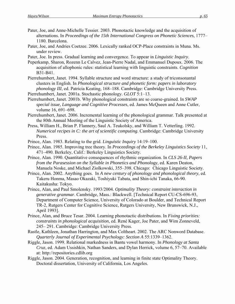
Hayes/Wilson Maximum Entropy Phonotactics p. 65
Pater, Joe, and Anne-Michelle Tessier. 2003. Phonotactic knowledge and the acquisition of alternations. In Proceedings of the 15th International Congress on Phonetic Sciences, 1777–1180. Barcelona.
Pater, Joe, and Andries Coetzee. 2006. Lexically ranked OCP-Place constraints in Muna. Ms. under review.
Pater, Joe. In press. Gradual learning and convergence. To appear in Linguistic Inquiry. Peperkamp, Sharon, Rozenn Le Calvez, Jean-Pierre Nadal, and Emmanuel Dupoux. 2006. The
acquisition of allophonic rules: statistical learning with linguistic constraints. Cognition B31-B41.
Pierrehumbert, Janet. 1994. Syllable structure and word structure: a study of triconsonantal clusters in English. In Phonological structure and phonetic form: papers in laboratory phonology III, ed. Patricia Keating, 168–188. Cambridge: Cambridge University Press.
Pierrehumbert, Janet. 2001a. Stochastic phonology. GLOT 5:1–13. Pierrehumbert, Janet. 2001b. Why phonological constraints are so coarse-grained. In SWAP
special issue, Language and Cognitive Processes, ed. James McQueen and Anne Cutler, volume 16, 691–698.
Pierrehumbert, Janet. 2006. Incremental learning of the phonological grammar. Talk presented at the 80th Annual Meeting of the Linguistic Society of America.
Press, William H., Brian P. Flannery, Saul A. Teukolsky, and William T. Vetterling. 1992. Numerical recipes in C: the art of scientific computing. Cambridge: Cambridge University Press.
Prince, Alan. 1983. Relating to the grid. Linguistic Inquiry 14:19–100. Prince, Alan. 1985. Improving tree theory. In Proceedings of the Berkeley Linguistics Society 11,
471–490. Berkeley, Calif.: Berkeley Linguistics Society. Prince, Alan. 1990. Quantitative consequences of rhythmic organization. In CLS 26-II, Papers
from the Parasession on the Syllable in Phonetics and Phonology, ed. Karen Deaton, Manuela Noske, and Michael Ziolkowski, 355–398. Chicago: Chicago Linguistic Society.
Prince, Alan. 2002. Anything goes. In A new century of phonology and phonological theory, ed. Takeru Honma, Masao Okazaki, Toshiyuki Tabata, and Shin-ichi Tanaka, 66-90. Kaitakusha: Tokyo.
Prince, Alan, and Paul Smolensky. 1993/2004. Optimality Theory: constraint interaction in generative grammar. Cambridge, Mass.: Blackwell. [Technical Report CU-CS-696-93, Department of Computer Science, University of Colorado at Boulder, and Technical Report TR-2, Rutgers Center for Cognitive Science, Rutgers University, New Brunswick, N.J., April 1993].
Prince, Alan, and Bruce Tesar. 2004. Learning phonotactic distributions. In Fixing priorities: constraints in phonological acquisition, ed. René Kager, Joe Pater, and Wim Zonneveld, 245– 291. Cambridge: Cambridge University Press.
Rastle, Kathleen, Jonathan Harrington, and Max Coltheart. 2002. The ARC Nonword Database. Quarterly Journal of Experimental Psychology: Section A 55:1339–1362.
Riggle, Jason. 1999. Relational markedness in Bantu vowel harmony. In Phonology at Santa Cruz, ed. Adam Ussishkin, Nathan Sanders, and Dylan Herrick, volume 6, 57–70. Available at: http://repositories.cdlib.org
Riggle, Jason. 2004. Generation, recognition, and learning in finite state Optimality Theory. Doctoral dissertation, University of California, Los Angeles.
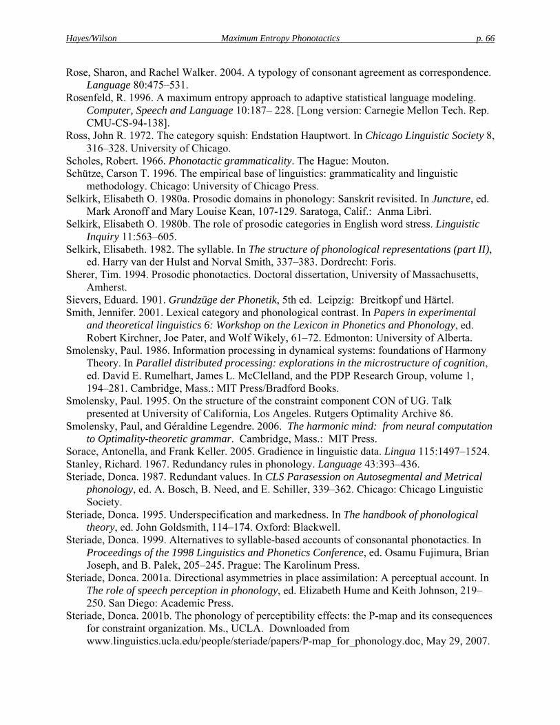
Hayes/Wilson Maximum Entropy Phonotactics p. 66
Rose, Sharon, and Rachel Walker. 2004. A typology of consonant agreement as correspondence. Language 80:475–531.
Rosenfeld, R. 1996. A maximum entropy approach to adaptive statistical language modeling. Computer, Speech and Language 10:187– 228. [Long version: Carnegie Mellon Tech. Rep. CMU-CS-94-138].
Ross, John R. 1972. The category squish: Endstation Hauptwort. In Chicago Linguistic Society 8, 316–328. University of Chicago.
Scholes, Robert. 1966. Phonotactic grammaticality. The Hague: Mouton. Schütze, Carson T. 1996. The empirical base of linguistics: grammaticality and linguistic
methodology. Chicago: University of Chicago Press. Selkirk, Elisabeth O. 1980a. Prosodic domains in phonology: Sanskrit revisited. In Juncture, ed.
Mark Aronoff and Mary Louise Kean, 107-129. Saratoga, Calif.: Anma Libri. Selkirk, Elisabeth O. 1980b. The role of prosodic categories in English word stress. Linguistic
Inquiry 11:563–605. Selkirk, Elisabeth. 1982. The syllable. In The structure of phonological representations (part II),
ed. Harry van der Hulst and Norval Smith, 337–383. Dordrecht: Foris. Sherer, Tim. 1994. Prosodic phonotactics. Doctoral dissertation, University of Massachusetts,
Amherst. Sievers, Eduard. 1901. Grundzüge der Phonetik, 5th ed. Leipzig: Breitkopf und Härtel. Smith, Jennifer. 2001. Lexical category and phonological contrast. In Papers in experimental
and theoretical linguistics 6: Workshop on the Lexicon in Phonetics and Phonology, ed. Robert Kirchner, Joe Pater, and Wolf Wikely, 61–72. Edmonton: University of Alberta.
Smolensky, Paul. 1986. Information processing in dynamical systems: foundations of Harmony Theory. In Parallel distributed processing: explorations in the microstructure of cognition, ed. David E. Rumelhart, James L. McClelland, and the PDP Research Group, volume 1, 194–281. Cambridge, Mass.: MIT Press/Bradford Books.
Smolensky, Paul. 1995. On the structure of the constraint component CON of UG. Talk presented at University of California, Los Angeles. Rutgers Optimality Archive 86.
Smolensky, Paul, and Géraldine Legendre. 2006. The harmonic mind: from neural computation to Optimality-theoretic grammar. Cambridge, Mass.: MIT Press.
Sorace, Antonella, and Frank Keller. 2005. Gradience in linguistic data. Lingua 115:1497–1524. Stanley, Richard. 1967. Redundancy rules in phonology. Language 43:393–436. Steriade, Donca. 1987. Redundant values. In CLS Parasession on Autosegmental and Metrical
phonology, ed. A. Bosch, B. Need, and E. Schiller, 339–362. Chicago: Chicago Linguistic Society.
Steriade, Donca. 1995. Underspecification and markedness. In The handbook of phonological theory, ed. John Goldsmith, 114–174. Oxford: Blackwell.
Steriade, Donca. 1999. Alternatives to syllable-based accounts of consonantal phonotactics. In Proceedings of the 1998 Linguistics and Phonetics Conference, ed. Osamu Fujimura, Brian Joseph, and B. Palek, 205–245. Prague: The Karolinum Press.
Steriade, Donca. 2001a. Directional asymmetries in place assimilation: A perceptual account. In The role of speech perception in phonology, ed. Elizabeth Hume and Keith Johnson, 219–250. San Diego: Academic Press.
Steriade, Donca. 2001b. The phonology of perceptibility effects: the P-map and its consequences for constraint organization. Ms., UCLA. Downloaded from www.linguistics.ucla.edu/people/steriade/papers/P-map_for_phonology.doc, May 29, 2007.
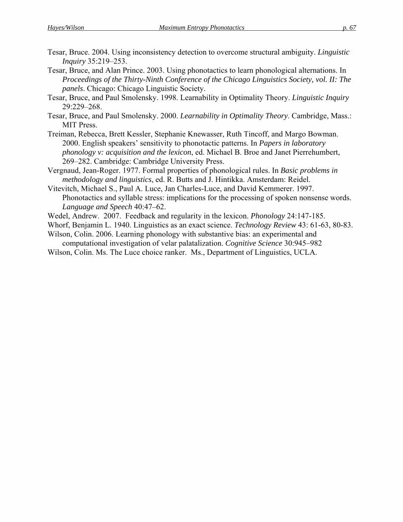
Hayes/Wilson Maximum Entropy Phonotactics p. 67
Tesar, Bruce. 2004. Using inconsistency detection to overcome structural ambiguity. Linguistic Inquiry 35:219–253.
Tesar, Bruce, and Alan Prince. 2003. Using phonotactics to learn phonological alternations. In Proceedings of the Thirty-Ninth Conference of the Chicago Linguistics Society, vol. II: The panels. Chicago: Chicago Linguistic Society.
Tesar, Bruce, and Paul Smolensky. 1998. Learnability in Optimality Theory. Linguistic Inquiry 29:229–268.
Tesar, Bruce, and Paul Smolensky. 2000. Learnability in Optimality Theory. Cambridge, Mass.: MIT Press.
Treiman, Rebecca, Brett Kessler, Stephanie Knewasser, Ruth Tincoff, and Margo Bowman. 2000. English speakers’ sensitivity to phonotactic patterns. In Papers in laboratory phonology v: acquisition and the lexicon, ed. Michael B. Broe and Janet Pierrehumbert, 269–282. Cambridge: Cambridge University Press.
Vergnaud, Jean-Roger. 1977. Formal properties of phonological rules. In Basic problems in methodology and linguistics, ed. R. Butts and J. Hintikka. Amsterdam: Reidel.
Vitevitch, Michael S., Paul A. Luce, Jan Charles-Luce, and David Kemmerer. 1997. Phonotactics and syllable stress: implications for the processing of spoken nonsense words. Language and Speech 40:47–62.
Wedel, Andrew. 2007. Feedback and regularity in the lexicon. Phonology 24:147-185. Whorf, Benjamin L. 1940. Linguistics as an exact science. Technology Review 43: 61-63, 80-83. Wilson, Colin. 2006. Learning phonology with substantive bias: an experimental and
computational investigation of velar palatalization. Cognitive Science 30:945–982 Wilson, Colin. Ms. The Luce choice ranker. Ms., Department of Linguistics, UCLA.