a mechanistic model for co localized corrosion of carbon steel mechanistic model for co2... ·...
TRANSCRIPT
A Mechanistic Model for CO2
Localized Corrosion of Carbon Steel
A dissertation presented to
the faculty of
the Russ College of Engineering and Technology of Ohio University
In partial fulfillment
of the requirements for the degree
Doctor of Philosophy
Hui Li
June 2011
© 2011 Hui Li. All Rights Reserved.
2
This dissertation titled
A Mechanistic Model for CO2
Localized Corrosion of Carbon Steel
by
HUI LI
has been approved for
the Department of Chemical and Biomolecular Engineering
and the Russ College of Engineering and Technology by
Srdjan Nešić
Professor of Chemical and Biomolecular Engineering
Dennis Irwin
Dean, Russ College of Engineering and Technology
3
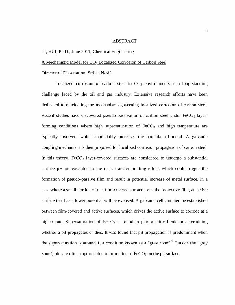
ABSTRACT
LI, HUI, Ph.D., June 2011, Chemical Engineering
A Mechanistic Model for CO2 Localized Corrosion of Carbon Steel
Director of Dissertation: Srdjan Nešić
Localized corrosion of carbon steel in CO2 environments is a long-standing
challenge faced by the oil and gas industry. Extensive research efforts have been
dedicated to elucidating the mechanisms governing localized corrosion of carbon steel.
Recent studies have discovered pseudo-passivation of carbon steel under FeCO3 layer-
forming conditions where high supersaturation of FeCO3 and high temperature are
typically involved, which appreciably increases the potential of metal. A galvanic
coupling mechanism is then proposed for localized corrosion propagation of carbon steel.
In this theory, FeCO3 layer-covered surfaces are considered to undergo a substantial
surface pH increase due to the mass transfer limiting effect, which could trigger the
formation of pseudo-passive film and result in potential increase of metal surface. In a
case where a small portion of this film-covered surface loses the protective film, an active
surface that has a lower potential will be exposed. A galvanic cell can then be established
between film-covered and active surfaces, which drives the active surface to corrode at a
higher rate. Supersaturation of FeCO3 is found to play a critical role in determining
whether a pit propagates or dies. It was found that pit propagation is predominant when
the supersaturation is around 1, a condition known as a “grey zone”.1 Outside the “grey
zone”, pits are often captured due to formation of FeCO3 on the pit surface.
4
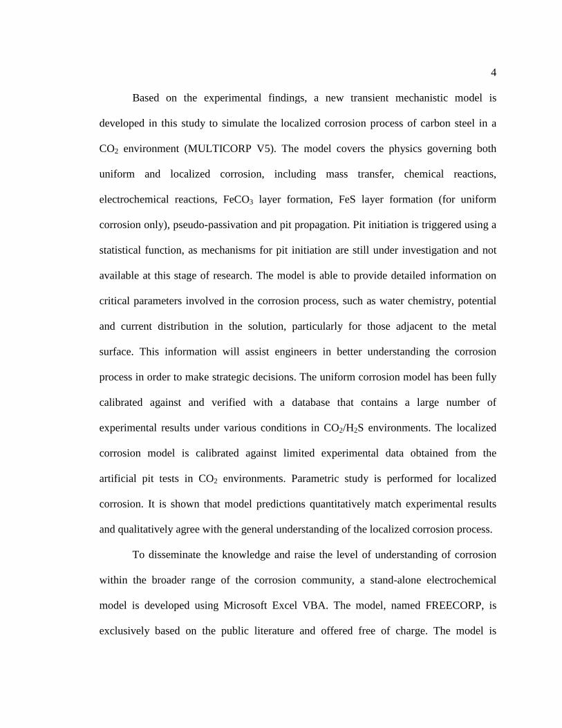
Based on the experimental findings, a new transient mechanistic model is
developed in this study to simulate the localized corrosion process of carbon steel in a
CO2 environment (MULTICORP V5). The model covers the physics governing both
uniform and localized corrosion, including mass transfer, chemical reactions,
electrochemical reactions, FeCO3 layer formation, FeS layer formation (for uniform
corrosion only), pseudo-passivation and pit propagation. Pit initiation is triggered using a
statistical function, as mechanisms for pit initiation are still under investigation and not
available at this stage of research. The model is able to provide detailed information on
critical parameters involved in the corrosion process, such as water chemistry, potential
and current distribution in the solution, particularly for those adjacent to the metal
surface. This information will assist engineers in better understanding the corrosion
process in order to make strategic decisions. The uniform corrosion model has been fully
calibrated against and verified with a database that contains a large number of
experimental results under various conditions in CO2/H2S environments. The localized
corrosion model is calibrated against limited experimental data obtained from the
artificial pit tests in CO2 environments. Parametric study is performed for localized
corrosion. It is shown that model predictions quantitatively match experimental results
and qualitatively agree with the general understanding of the localized corrosion process.
To disseminate the knowledge and raise the level of understanding of corrosion
within the broader range of the corrosion community, a stand-alone electrochemical
model is developed using Microsoft Excel VBA. The model, named FREECORP, is
exclusively based on the public literature and offered free of charge. The model is

5 capable of predicting steady-state CO2 and/or HAc uniform corrosion and transient H2S
uniform corrosion for carbon steel. Apart from corrosion rate prediction, polarization
curves can also be predicted for individual and overall electrochemical reactions in order
to enhance understanding of corrosion mechanisms. In the case of H2S corrosion, the
concentration profile of H2S across the inner and outer makinawite film and bulk solution
is shown in order to give more meaningful information about H2S corroison. This model
is written with the concept of object-oriented programming (OOP) which provides great
flexibility to model calculations. Any reactions, including system-defined and user-
defined reactions, can be added or removed from the system, a feature that allows for
investigation into the effect of individual reactions on the corrosion process. This feature
also permits the expansion of the model into a much wider range of environments than
the model was originally designed for. The current model is fully calibrated and verified
with a large number of in-house experimental data contained in the ICMT (Institute for
Corrosion and Multiphase Flow Technology at Ohio University) database.
Approved: _____________________________________________________________
Srdjan Nešić
Professor of Chemical and Biomolecular Engineering

6
DEDICATION
To
Guangyou Li and Piyu Yan (my parents)
and
Jun Luo (my wife)
7
ACKNOWLEDGMENTS
I would like to express my sincere gratitude to my advisor and chairman of my
dissertation committee, Dr. Srdjan Nešić, for his constant guidance and support during
my PhD studies. His direction and encouragement are among the key factors for the
completion of my PhD degree. Apart from being an esteemed professor and a well-
known expert, he also showed great care for issues pertaining to my everyday life. I am
so grateful for his willingness to help whenever I approached him with a “problem”.
I would like to acknowledge my project leader, Mr. Bruce Brown, for his help
with my experimental work and valuable suggestions on my project. Assistance was also
provided by Dr. Dusan Sormaz with modeling work and by Dr. Yoon-Seok Choi with
model verification, which are greatly appreciated. My gratitude is extended to other
committee members, Dr. Michael Prudich, Dr. Howard Dewald and Dr. Michael Jensen,
for their agreement to serve on my dissertation committee.
I would like to acknowledge Ms. Jing Huang and Mr. Danyu You for their help
during the model development, especially in the development of FREECORP. I greatly
appreciate all the staff and fellow students in this institute for their cooperation and
assistance, which has made my stay an enjoyable experience. Special thanks go to the
CCJIP sponsoring companies for their financial and technical support.
I would like to convey my heartfelt gratitude to my parents for their
unconditional love and encouragement. A last but not least thanks go to my wife for her
love, sacrifice and devotion to my family, without which I could have never made this
far.
8
TABLE OF CONTENTS
Page Abstract ................................................................................................................................3
Dedication ............................................................................................................................6
Acknowledgments................................................................................................................7
List of Tables .....................................................................................................................11
List of Figures ....................................................................................................................12
Chapter 1: Introduction ......................................................................................................17
Chapter 2: Literature Review .............................................................................................21
2.1 Passivation ...............................................................................................................22
2.2 Pit initiation ..............................................................................................................29
2.3 Pit propagation .........................................................................................................43
Chapter 3: Research Objectives .........................................................................................58
Chapter 4: Mechanistic Model of Localized CO2 Corrosion .............................................61
4.1 Introduction ..............................................................................................................61
4.2 Physico-chemical Processes Described by the Model .............................................63
4.3 Physico-chemical Model ..........................................................................................68
4.3.1 Chemical Reactions ..........................................................................................68
4.3.2 Electrochemical reactions .................................................................................72
4.3.3 Mass transport ...................................................................................................75
4.3.4 FeCO3 precipitation ..........................................................................................77
4.3.5 Pseudo-passivation ............................................................................................78
4.3.6 Depassivation and pit initiation ........................................................................80
4.3.7 Repassivation and pit death...............................................................................81
4.3.8 Pit propagation ..................................................................................................82
4.4 Mathematical Model ................................................................................................84
4.4.1 Chemical reactions ............................................................................................84
4.4.2 Electrochemical reactions .................................................................................89
4.4.3 Mass transport .................................................................................................104
4.4.4 FeCO3 layer Growth .......................................................................................110

9
4.4.5 Pseudo-passivation/repassivation....................................................................115
4.4.6 Pit initiation .....................................................................................................118
4.4.7 Pit propagation ................................................................................................120
4.5 Numerical technique ..............................................................................................124
4.6 Solving strategy .....................................................................................................130
4.7 Model verification and parametric study ...............................................................133
4.7.1 Uniform corrosion verification .......................................................................134
4.7.2 Localized corrosion verification .....................................................................137
4.7.3 Parametric study ..............................................................................................146
4.8 Model limitations ...................................................................................................152
5. Conclusions .............................................................................................................153
References ........................................................................................................................156
Appendix 1: Derivation of the Equation for FeCO3 layer Dissolution ............................168
Appendix 2: Derivation of the Exchange Current Density for Iron Oxidation ................170
Appendix 3: Derivation of the Exchange Current Density for H+ Reduction .................173
Appendix 4: Determination of the Environmental Parameters Affecting Pseudo-Passive Current Density of Carbon Steel by Cyclic Polarization Technique ...............................176
A4.1 Test Procedure and Test Matrix ..........................................................................176
A4.2 Test Results .........................................................................................................178
A4.3 Test Result Analysis ...........................................................................................183
Appendix 5: Modeling Pseudo-Passive Current Density of Carbon Steel in CO2 Environment Based on Point Defect Model ....................................................................185
A5.1 Introduction .........................................................................................................185
A5.2 Model Development ............................................................................................187
Appendix 6: Open Source Model of Uniform CO2/H2S Corrosion .................................196
A6.1 Introduction .........................................................................................................196
A6.2 Theories of the Model .........................................................................................198
A6.3 Mathematical Model ...........................................................................................200
A6.3.1 CO2/HAc Corrosion .....................................................................................201
A6.3.2 H2S Corrosion ..............................................................................................210
A6.3.3 Film Growth .................................................................................................214
A6.3.4 Determination of CO2/H2S Dominant Process .............................................215

10
A6.4 Implementation of the Model ..............................................................................215
A6.5 Model Limitations ...............................................................................................221
A6.6 Model Verification ..............................................................................................222
A6.7 Conclusions .........................................................................................................229

11
LIST OF TABLES
Page Table 1. The electrochemical parameters used for Tafel equation* in the previous model
where the current density is calculated as ..........................................94
Table 2. The electrochemical parameters used for Butler-Volmer equation* in the current model where current density is calculated as ....................95
Table 3. Effect of factors on pseudo-passive current density ..........................................102
Table 4. Species commonly existing in the system of interest, and the corresponding diffusion coefficient at 25°C ............................................................................................106
Table 7. Test conditions for cyclic polarization test ........................................................177
Table 8. Test matrix for factorial design experiments .....................................................178
Table 9. Summary of the results for cyclic polarization tests ..........................................182
Table 10. Matrix used for performing factorial effect analysis .......................................184
Table 6. Test conditions taken from open literature132 for FREECORP verification ......228

12
LIST OF FIGURES
Page Figure 1. Place exchange mechanism proposed by Sato and Cohen.24 M: metal ion; O: oxygen ion. .........................................................................................................................23
Figure 2. Mechanism proposed by Marcus et al. 66 for local breakdown of passivity driven by the potential drop at the oxide/electrolyte interface of an inter-granular boundary of the barrier layer. The effect of chlorides is shown. .......................................40
Figure 3. Mechanisms proposed by Marcus et al. 66 for local breakdown of passivity driven by the potential drop at the metal/oxide interface of an inter-granular boundary of the barrier layer. The effect of ion transport is shown: (a) predominant cation transport and (b) predominant anion diffusion..................................................................................41
Figure 4. Illustration of corrosion process: FeCO3 layer formation leading to surface pH increases. ............................................................................................................................65
Figure 5. Illustration of corrosion process: pseudo-passivation leading to potential increases. ............................................................................................................................65
Figure 6. Illustration of corrosion process: depassivation leading to separation of anode and cathode and establishment of potential difference. .....................................................66
Figure 7. Illustration of corrosion process: Pit propagation. .............................................66
Figure 8. Illustration of corrosion process: FeCO3 re-precipitation if superstaturation of FeCO3 is sufficiently high. .................................................................................................67
Figure 9. Illustration of corrosion process: Repassivation leading to pit death. ...............67
Figure 10. The Pourbaix diagram for Fe/CO2/H2O system with temperature 80°C, [Fe2+]1ppm. Courtesy of T. Tanupabrungsun. ...................................................................80
Figure 11. Illustration of potential distribution in a galvanic cell. represents the solution potential drop across the double layer, represents the electrode potential at different locations, represents metal potential. ....................................................84
Figure 12. Potential/current distribution predicted by the Tafel equation.........................92
Figure 13. Potential/current distribution predicted by the Butler-Volmer equation. ........93
Figure 14. Potentiodynamic sweep on stainless steel and carbon steel. Test condition: T=25°C, pH=4.1, pCO2=1 bar, stagnant solution. .............................................................99
Figure 15. Comparison of potentiodynamic sweep of stainless steel with polarization curves of carbon steel generated from the software. Test conditions: T=25°C, pH=4, NaCl=1%, stagnant solution. ...........................................................................................100
13 Figure 16. Comparison of potentiodynamic sweep of stainless steel with Polarization curves of carbon steel generated from FREECORP. Test condition: T=25°C, pH=5, NaCl=1%, stagnant solution. ...........................................................................................100
Figure 17. Illustration of computation domain and governing equation for mass transport simulation. ........................................................................................................................110
Figure 18. Comparison of surface porosity of FeCO3 layer with different high-order schemes for convective term in Equation (95). Simulation condition: temperature 80°C, CO2 partial pressure 1 bar, liquid velocity1m/s, pipe diameter 0.1m, bulk super saturation of FeCO3 about 0.5 and bulk pH 6.5. ...............................................................................113
Figure 19. Comparison of corrosion rate with different high-order schemes for convective term in Equation (95). Simulation condition: temperature 80°C, CO2 partial pressure 1 bar, liquid velocity1m/s, pipe diameter 0.1m, bulk super saturation of FeCO3 about 0.5 and bulk pH 6.5. ...............................................................................................113
Figure 20. Illustration of computation domain and governing equation for FeCO3 layer growth simulation. ...........................................................................................................114
Figure 21. Computation domain and governing equation with boundary conditions for electrostatic potential distribution in aqueous solution. ...................................................123
Figure 22. Schematic of control volumes used for discretizing the governing equations for mass transport and FeCO3 layer growth.13 .................................................................126
Figure 23. Schematic of the 2-D control volumes used for discretizing governing equations for potential distribution. .................................................................................129
Figure 24. Flow chart used in the localized corrosion model..........................................132
Figure 25. Comparisons between model and experiments for 1 bar CO2, 20°C and various pHs and velocities. ..............................................................................................135
Figure 26. Comparison between model and experiments for FeCO3 layer forming condition at temperature 80°C, 0.53bar CO2, pH 6.3 and bulk Fe2+ concentration 50ppm, stagnant. ...........................................................................................................................136
Figure 27. Comparisons between the model and the experiments for flowing FeCO3 layer-forming condition at temperature 80°C, pH 6.6, 0.53bar CO2, 10ppm bulk Fe2+ and 1000rpm rotation speed....................................................................................................137
Figure 28. Schematic illustration of the artificial pit unit used in Han et al. experiments (a) fully assembled artificial pit, (b) cutaway side view, (c) enlarged bottom view of cathode; center hole for anode, (d) detailed cross section view.105 .................................139
Figure 29. Evans diagram depicting relationship of galvanic current and anodic current. Galvanic current is represented by Igalvanic and anodic current is symbolized by Icorr
couple.140
Figure 30. Comparison of anodic current density and galvanic current density. Simulation conditions: Supersaturation of FeCO3 0.3−0.9, T 80 ºC, CO2 0.53bar, pH 5.9-6.1, 1wt % NaCl, stagnant. ..............................................................................................140
14 Figure 31. Comparison of galvanic current density between model and experiments for the conditions: Supersaturation of FeCO3 0.3−0.9, Temperature 80 ºC, CO2 0.53bar, pH 5.9-6.1, 1wt % NaCl, stagnant. ........................................................................................142
Figure 32. Surface pH and potential as a function of time. Simulation conditions: Supersaturation of FeCO3 0.3−0.9, T 80 ºC, CO2 0.53bar, pH 5.9-6.1, 1wt % NaCl, stagnant. ...........................................................................................................................143
Figure 33. Comparison between the model and the experiment for the conditions: Supersaturation of FeCO3 3−9, T 80 ºC, pCO2 0.53bar, pH 5.6, [NaCl] =1wt%, stagnant.144
Figure 34. Comparison between model and experiments for the conditions: Supersaturation of FeCO3 0.8−4, T 80 ºC, CO2 0.53bar, pH 5.9, 1wt % NaCl, 500rpm.145
Figure 35. Anode surface pH vs. time for the condition: Supersaturation of FeCO3 0.8−4, T 80 ºC, CO2 0.53bar, pH 5.9, 1wt % NaCl, 500rpm. .....................................................146
Figure 36. Effect of supersaturation on localized corrosion rate. Simulation conditions: temperature 80°C, CO2 partial pressure 0.52bar, 0.1 wt% NaCl, velocity 0.2m/s, bulk pH 6........................................................................................................................................148
Figure 37. Potential difference between anode and cathode for two simulation cases with supersaturation 1 and 10 respectively. Simulation conditions: temperature 80°C, CO2 partial pressure 0.52bar, 0.1 wt% NaCl, velocity 0.5m/s, bulk pH 6. .............................149
Figure 38. Corrosion rate comparison for bulk liquid velocity at 0.5m/s and 1m/s. Simulation conditions: temperature 80°C, CO2 partial pressure 0.52bar, 0.1 wt% NaCl, bulk pH 6, bulk supersaturation of FeCO3 10. .................................................................151
Figure 39. Galvanic current densities for solutions with different conductivity. Simulation conditions: pH 5.9, T 80°C, CO2 0.53bar, FeCO3 supersaturation 2, 0.25m/s.152
Figure 40. E-i diagram for Fe oxidation. irev can be obtained from the point (E0, i0), the Tafel slope ba and Erev. .....................................................................................................172
Figure 41. E-i diagram for H+ reduction. irev can be obtained from the point (E0, i0), the Tafel slope bc and Erev. .....................................................................................................175
Figure 42. Cyclic polarization curve of C1018. Test conditions: T=60°C, pH=7, NaCl=0.2 mol/L. ..............................................................................................................178
Figure 43. Cyclic polarization curve of C1018. Test conditions: T=60°C, pH=8, NaCl=0.2 mol/L. ..............................................................................................................179
Figure 44. Cyclic polarization curve of C1018. Test conditions: T=80°C, pH=7, NaCl=0.2 mol/L. ..............................................................................................................179
Figure 45. Cyclic polarization curve of C1018. Test conditions: T=80°C, pH=8, NaCl=0.2 mol/L. ..............................................................................................................180
Figure 46. Cyclic polarization curve of C1018. Test conditions: T=60°C, pH=7, NaCl=2 mol/L. ...............................................................................................................................180

15 Figure 47. Cyclic polarization curve of C1018. Test conditions: T=60°C, pH=8, NaCl=2 mol/L. ...............................................................................................................................181
Figure 48. Cyclic polarization curve of C1018. Test conditions: T=80°C, pH=7, NaCl=2 mol/L. ...............................................................................................................................181
Figure 49. Cyclic polarization curve of C1018. Test conditions: T=80°C, pH=8, NaCl=2 mol/L. ...............................................................................................................................182
Figure 50. Illustration of the Schottky(a) and Frenkel(b) defects by Gao.137 ..................187
Figure 51. Original point defect model for carbon steel.38 Fe: Fe atom on a metal lattice site; FeFe: Fe on Fe site in the oxide; Fei
χ+: iron interstitial in the oxide layer; OO: oxygen ion in the oxide; VFe
χ’= Fe vacancy; VO..= oxygen vacancy; FeГ+: metallic species in
solution; FeOχ/2: oxide barrier layer; FeCO3: precipitated outer layer; ki : reaction rate constant; BL: oxide barrier layer; OL: outer layer..........................................................188
Figure 52. Point Defect Model proposed in this work. Fe: Fe atom on a metal lattice site; FeFe: Fe on Fe site in the oxide; OO: oxygen ion in the oxide; VFe
3-: Fe vacancy; VO2+:
oxygen vacancy; Fe2++: metallic species in solution; FeO3/2: oxide barrier layer; ki : reaction rate constant; BL: oxide barrier layer; S: solution. ...........................................189
Figure 53. Structure of the FREECORP software.16 .......................................................216
Figure 54. Screen shot for contributions of corrosive species in a CO2 corrosion case. Simulation conditions: temperature 20°C, pipe diameter 0.1m, velocity 1m/s, CO2 partial pressure 1bar, HAc 10ppm, pH 4.....................................................................................217
Figure 55. Screen shot for contributions of corrosive species in a H2S corrosion case. Simulation conditions: temperature 20°C, pipe diameter 0.1m, velocity 1m/s, CO2 partial pressure 1bar, H2S 10ppm, pH 4. .....................................................................................218
Figure 56. Screen shot for the user input/output window for CO2 corrosion in FREECORP. ....................................................................................................................219
Figure 57. Screen shot for the user input/output window for H2S corrosion in FREECORP. ....................................................................................................................220
Figure 58. Template for the inputs of a user-defined reaction in FREECORP. ..............221
Figure 59. Comparison of experimental and FREECORP predicted polarization curves for temperature 20°C , partial pressure of CO2 1bar, solution pH 4 and velocity 2 m/s.16223
Figure 60. Comparison between FREECORP predictions and experiments for different partial pressure of CO2. Test condition: temperature 60°C, pH 5, pipe diameter 0.1 m. Data is taken from ICMT database.16 ..............................................................................225
Figure 61. Comparison of experimental and FREECORP predicted corrosion rate. Test conditions: temperature 60°C, pH 5, liquid velocity 1 m/s, partial pressure of CO2 10 bar, pipe diameter 0.1m.16 .......................................................................................................226

16 Figure 62. Comparison of FREECORP predictions and measurements for H2S corrosion. Test conditions: temperature 80°C, pH 5, liquid velocity 1 m/s, pipe diameter 0.1m. Data is taken from icmt database.16 ..........................................................................................227
Figure 63. Comparison of measured and FREECORP predicted corrosion rates under the conditions listed in Table 10.16 ........................................................................................228

17
CHAPTER 1: INTRODUCTION
Carbon steel is one of the most widely used engineering constructional materials
due to its low cost and relatively good mechanical properties. This is particularly true in
the oil and gas industry where transportation of products predominantly relies on
pipelines spanning thousands of miles. In such cases, corrosion resistant alloys (CRAs)
are not cost-efficient considering the large amount of materials involved in the
construction. The use of carbon steels, when combined with other protective measures
such as corrosion inhibitors, cathodic protection, non-metallic paints or CRA claddings,
is the most common ways to satisfy the transportation needs of the oil and gas industry.
Unlike CRAs, which are protected by the surface passive film spontaneously formed in
the air, carbon steel surface is active in most corrosive media, which often leads to an
unacceptably high corrosion rate. Clearly, the corrosion of carbon steels represents a
major concern in their industrial applications. Uniform and localized corrosion are the
two most common types of corrosion in carbon steel.2 In most cases, uniform corrosion
can be efficiently controlled by various corrosion inhibition methods as parts of a
properly maintained corrosion management program. Localized corrosion, however,
poses a much greater threat to the integrity of carbon steel pipelines. This is due to the
stochastic and seemingly unpredictable induction period associated with localized
corrosion and the fact that once initiation occurs, some pits can propagate at a much
higher rate compared to uniform corrosion. Therefore, localized corrosion of carbon steel
can significantly reduce the lifetime of pipelines, and increase the costs by increasing the
frequency of replacing or repairing facilities and interrupting oil and gas production.
18
To combat corrosion, significant efforts have been made in the past few decades
towards understanding the corrosion of carbon steel in the oil and gas industry. Thanks to
past study, the mechanisms governing uniform CO2 corrosion of carbon steel (especially
without the presence of precipitates such as iron carbonate (FeCO3) and other less soluble
salts) are now well understood. As a result, a number of corrosion models have been
developed to predict uniform CO2 corrosion of carbon steel.3 These models typically
exhibit good agreement in “bare” steel corrosion conditions, but they deviate from each
other when the protective FeCO3 layer is present on the steel surface.4 The difficulty of
modelling FeCO3 layer growth is the main cause for these prediction deviations.
Different strategies have been proposed by various modellers to account for the FeCO3
effect. Most models incorporate an empirical factor into the corrosion calculations; some
determine FeCO3 effect based on thermodynamic criteria while others simulate FeCO3
layer growth kinetics. Although no consensus has been reached as to the strategy for
modelling the FeCO3 layer effect, a satisfactory corrosion prediction can be achieved if
the models are carefully calibrated with good source of experiment data.
At present, most uniform corrosion models are proprietary and unavailable to the
public. The corrosion prediction tool available to the corrosion community at large is
limited to a few empirical and semi-empirical models, such as de Waard-Milliams
model5-8, Norsok model9,10 etc., which were developed based on individual databases.
Application of these models in users’ unique corrosion situations poses some degree of
uncertainty as to the judgement of corrosion severity, particularly when the field
conditions fall outside the parameter range used for model development. A mechanistic
19 model, however, can be extrapolated to a much wider range of parameters due to sound
theoretical basis; therefore, it is able to provide corrosion prediction with a higher
confidence level. As part of the efforts to provide the corrosion community with an
additional tool for corrosion evaluation, a mechanistic model to predict uniform
CO2/HAc/H2S corrosion is developed in this project. This model, called FREECORP, is
built exclusively based on publicly available information and the source code is open for
maximum transparency. The model development is described in detail in Chapter 5.
Although uniform CO2 corrosion can now be predicted with reasonable
confidence, localized corrosion modelling remains as a more challenging topic. Despite
extensive research carried out in the past with the aim of understanding localized
corrosion of carbon steel, the mechanisms are still only partly understood. This is mainly
due to the complexity associated with pit initiation; a number of factors (pH, flow
disturbance, chloride concentration, etc.) have been proposed to induce pit initiation.
However, the stochastic nature of pit initiation makes any attempts to validate the
proposed theories difficult. In addition, the pits are typically inaccessible to common
experiment equipment due to geometrical restrictions, making it difficult to examine the
water chemistry inside the pit area, a property considered to be closely related to
localized corrosion.
In recent studies performed in the Institute for Corrosion and Multiphase
Technology at Ohio University (ICMT), an appreciable electrochemical potential
increase has been observed for carbon steel immersed in CO2 solutions after the build-up
of an FeCO3 layer.11 The potential increase is attributed to the generation of magnetite

20 leading to pseudo-passivation of the carbon steel surface.12 Due to the large potential
difference between active surface and film covered surfaces, a galvanic coupling
mechanism has been proposed for the propagation of localized corrosion of carbon
steel.11 Based on this mechanism, a transient mechanistic model is developed in the
present study to predict localized CO2 corrosion of carbon steel. The new model is built
from the “ground-up” however it is based on a previously developed uniform corrosion
model, MULTICORP, in which water chemistry, electrochemistry, mass transport and
FeCO3 layer formation are simulated according to corresponding physico-chemical
laws13,14. The unique phenomena for CO2 localized corrosion, such as pseudo-
passivation/repassivation, pit initiation and pit propagation are added into MULTICORP
in this study to enable prediction of both uniform and localized CO2 corrosion. With this
model, water chemistry in the pit area, particularly pH near the pit surface, can be
determined, and this can be utilized to facilitate the understanding of localized CO2
corrosion of carbon steel.
This document is structured as follows: the literature review is given in Chapter 2;
research objectives are laid out in Chapter 3; the localized corrosion model is presented in
Chapter 4. Relevant equation derivations and experiment details, and are presented in the
Appendix 1 to 5. A free mechanistic uniform corrosion model is described in Appendix 6.
It should be noted that parts of Chapter 4 for the localized corrosion model and Appendix
6 for the uniform corrosion model have been presented in two published papers.15,16
21
CHAPTER 2: LITERATURE REVIEW
The model discussed in this work is based on a galvanic coupling mechanism
where pseudo-passivation is proposed to be present on the cathode surface. For any
galvanic corrosion scenario, it is generally accepted that there are three important stages
involved: passivation, pit initiation and pit propagation. In the passivation stage, steel
surfaces are covered with passivating material(s) leading to a pronounced potential
increase and a dramatic decrease in the corrosion rate. In the pit initiation stage, passive
film is damaged in localized regions, leading to uncovered active surfaces with a lower
potential, which are electrically coupled with a passivated surface with a higher potential.
In the pit propagation stage, the potential difference between large passivated surfaces
(cathode) and small active surfaces (anode) drives an electrical current between the two
which makes the pit propagate. Under some conditions, however, the pit growth could be
arrested due to repassivation of the active surface(s). Each of these stages is governed by
unique mechanisms and must be treated separately.
A number of models have been developed in the past with the aim of simulating
one or multiple stages of localized corrosion. These models, most of which have been
developed for stainless steels and other passivating alloys, differ significantly in their
underlying mechanisms. A literature review is given in this chapter for localized
corrosion models in order to pave the path towards CO2 localized corrosion modelling of
carbon steel.

22 2.1 Passivation
Passivation is characteristic of a substantial corrosion current (rate) drop resulting
from a small increase in potential. The passive film formed on metal surface prohibits the
metal from actively reacting with a surrounding corrosive medium, and therefore
significantly reduces the corrosion rate. Passivation used to be considered a unique
feature for CRAs in the early stage of localized corrosion research. In recent years, it has
been discovered that passivation also takes place on carbon steel surfaces under
appropriate conditions12,17-22.
Fleischmann and Thirsk23 derived generic equations for calculating transient
current in the initial stage of metal passivation. By assuming cylindrical-shaped crystals,
the equations were developed to simulate two scenarios of passivated crystal growth,
namely growth of the discrete passivated crystal centers and two-dimensional growth of
mono-layer passivated crystal centers. The rate constants in the equations can be obtained
by making short-period potentiostatic measurements at the initial stage of passivation. It
was claimed that the difference in the two models relies on the assumption of crystal
growth due to a single nucleus vs. a large number of nuclei. A distribution function is
built in the model equations to account for random distribution of all possible forms of
crystals center overlapping.
Sato and Cohen24 developed an equation to calculate the passive iron growth
kinetics in neutral solutions. The model is proposed based on the assumption of “place-
exchange”, which suggests that growth of passive oxide film is a result of the oxygen
atom from OH- in water replacing the iron atom in the metal substrate. This process is
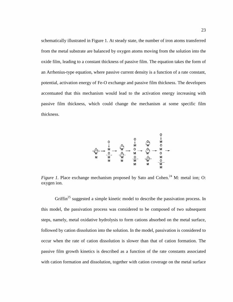
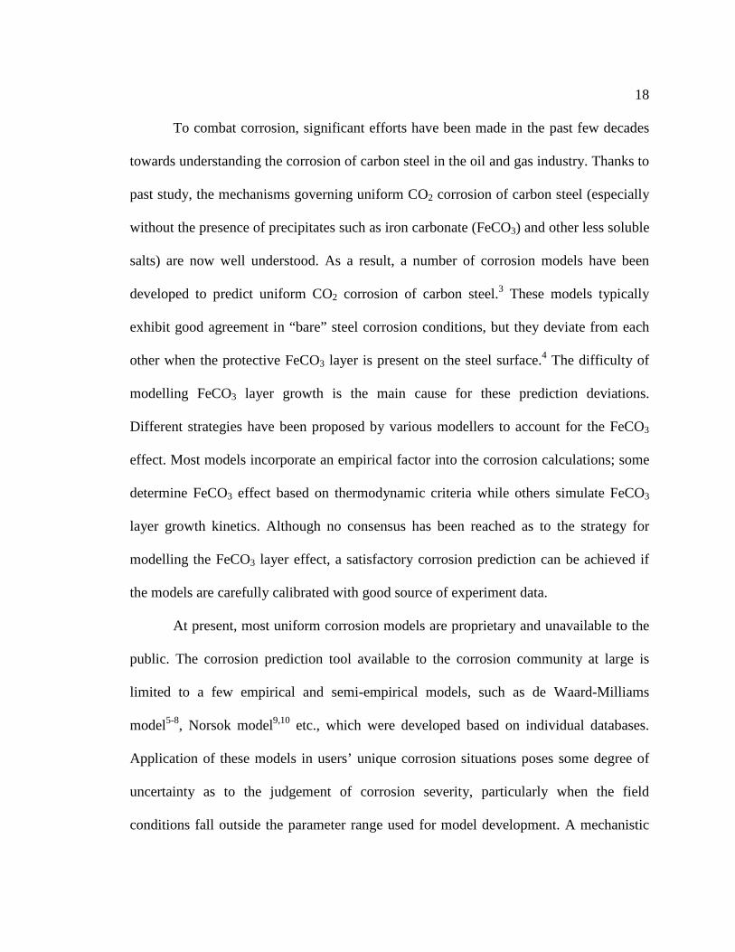
23 schematically illustrated in Figure 1. At steady state, the number of iron atoms transferred
from the metal substrate are balanced by oxygen atoms moving from the solution into the
oxide film, leading to a constant thickness of passive film. The equation takes the form of
an Arrhenius-type equation, where passive current density is a function of a rate constant,
potential, activation energy of Fe-O exchange and passive film thickness. The developers
accentuated that this mechanism would lead to the activation energy increasing with
passive film thickness, which could change the mechanism at some specific film
thickness.
Figure 1. Place exchange mechanism proposed by Sato and Cohen.24 M: metal ion; O: oxygen ion.
Griffin25 suggested a simple kinetic model to describe the passivation process. In
this model, the passivation process was considered to be composed of two subsequent
steps, namely, metal oxidative hydrolysis to form cations absorbed on the metal surface,
followed by cation dissolution into the solution. In the model, passivation is considered to
occur when the rate of cation dissolution is slower than that of cation formation. The
passive film growth kinetics is described as a function of the rate constants associated
with cation formation and dissolution, together with cation coverage on the metal surface

24 and the Tafel coefficient of metal oxidation. The model equation was shown to be able to
simulate the current-potential behaviour in the active-passive transition region.
Zakroczymski et al. 17 found that passive film formation on iron occurred in two
steps. In the initial step which lasted only a few seconds, passive film thickness reached
60-80% of its final value. Iron oxide/hydroxide, FeOOH, along with significant amount
of water, was found within the passive film. The amount of water decreased as the
passivation process continued, resulting in a much denser passive film in the second step,
where metal was much more resistant to pitting corrosion. The presence of water was
thought to play a significant role in passivity breakdown, as the continuous phase of
water provides a path for Fe2+ and Cl- to move through the passive film and also allows
hydrolysis reaction of Fe2+ to occur. The thickness of the passive film, on the other hand,
was not found to be important in passivation process.
Sarasola et al. 26 presented a layer-pore resistance model to explain the
experimentally-observed passivation of iron in 1M KOH solution in the cyclic
polarization test. In this model, passive film growth rate is calculated as a function of
polarization scan rate, passive film consumption rate and the total system resistance. The
total resistance is attributed to three components: active electrode surface, electrolyte and
passive film. The authors referred to the work of Devilliers et al.27 and suggested that the
active and passive behavior of iron polarization can be obtained using the model by
assuming the first and second orders of passive film consumption respectively. As shown
by the authors, this model is capable of simulating the current-potential behaviour in the
passive region for iron in KOH solution.
25
Macdonald and his colleagues proposed a so-called ‘Point Defect Model’ for
passive film growth in a series of published papers, initiating at the beginning of 1980s28-
31. In this model, passive film growth was hypothesized as a result of motions of various
defects (vacancies and/or interstitials) within the passive film. The whole process was
mathematically described by five equations accounting for five reactions that occur at
metal/film and film/solution interfaces. Vacancies/interstitials are considered participants
of these reactions. The most important assumptions made in this model include:
Passive film is composed of metal oxide, MOx/2 where high concentrations of
defects, particularly vacancies, are present. Passive film growth is attributed to the
transport of these defects.
The metal/passive film and passive film/solution are in electrochemical
equilibrium.
Electric field strength is independent of film thickness. This assumption has been
verified by experimental evidence, as the potential drop across the passive film
was found to be linearly changed with passive film thickness.32
Passive film/solution interface potential is linearly related to pH and applied
potential.
It was argued that this model is consistent with the well-established experimental
observations related to passivation.32 These observations include:
A passive film has a bi-layer structure with a highly disordered barrier adjacent to
the metal substrate and a less protective outer precipitated layer;

26 The passive film thickness and logarithmic passive current density are linearly
varied with the applied potential;
The inner passive film grows into the metal substrates while the outer passive film
grows outwards the solution.
Due to the capability of explaining the above-mentioned experimental results, the
Point Defect Model is considered to be one of the most successful passivation
models. Although originally developed for aluminium alloys, the theories
embedded in this model can be expanded to other metals such as carbon steel.
Proper electrochemical experiments need to be conducted in order to obtain
multiple constants in the model equations suitable for the materials of interest.
Hibbert and Murphy33 developed a minimal kinetic model to simulate corrosion
and passivity of iron. The model is based on the mechanisms proposed by Epelboin34 as
shown below:
(1)
(2)
(3) By expressing the rates of generation/consumption of each involved species,
[Fe(OH)]ads, [Fe(OH)2]ads and [OH-], as functions of rate constant, surface coverage ratio
and concentrations, a current-voltage relationship can be obtained. The model equations
are able to predict the current variations in the full range of potential, covering active,
passive and active-passive transition regions. A linear stability analysis indicated that the
model was stable in the active and passive regions of the current-potential curves and

27 became unstable in the transition region, which resulted in a periodic current-time
variation in this region. This indicates that the model requires external perturbation to
trigger passivity.
Pyun and Hong35 developed a model to simulate the passive film growth kinetics
by taking into account Fickian diffusion and migration of cation vacancy in the passive
film. The current density associated with passive film growth is calculated as a function
of electric field strength and film thickness, which evolves with time. In contrast to
Macdonald’s model where electric field strength is independent of applied potential, this
model suggests an increasing electric field strength with applied potential. However, no
experimental verification was given for the proposed functions, making the model less
convincing compared to Macdonald’s.
Meakin et al. 36 took a probabilistic approach to simulate passivation and
depassivation of metals subject to localized corrosion. A 2D square-lattice model was
developed in their work where sites of lattice are represented by four different states,
namely: unreactive fluid or corrosion product, corrosive fluids or particles, reactive metal
and unreactive passive metal. This model assumes a diffusion-limited corrosion process.
Passivation is considered to be a spontaneous random event characterized by a
passivation rate constant. At each time step, a randomly generated number between 0 and
1 is compared with a passivation probability function; a smaller random number would
lead to one of the reactive metal sites converted to a passive metal site, and vice versa.
Despite a lack of physical representation of the process, the model was shown to be able
to simulate some characteristic features of localized corrosion, including pit propagation,
28 pit death and current fluctuation. However, the authors also stressed that the model
cannot represent the real corrosion system, as the passivation rate constant, which is a
time-dependent variable, is taken as a constant in the model.
Reis et al. 37 proposed a stochastic model to simulate corrosion and passivation of
a metal based on the scaling theory. This model was designed to simulate the incubation
period during which transition from slow passivation to fast pit propagation occurs. The
model is simulating a 2D lattice where each site of lattice is represented by one of the six
possible states: bulk, reactive or passive metal and neutral, basic or acidic solution. In this
model, passivation, dissolution of passive film and spatially separated electrochemical
reactions are described by certain probabilistic rules. The model predicts the average
radius of passive film dissolution and average incubation time. It suggests that the
average radius decreases with the spatially separated electrochemical reaction rates and
dissolution rates in acidic media, but increases with the diffusion coefficients of H+ and
OH- in solution. The average incubation time is determined by the time characteristic of
slow passive film dissolution in neutral solutions until significant pH inhomogeneities are
established inside the pit. The model suggests that the average incubation time linearly
increases with the rate of dissolution.
Camacho et al. 38 developed an impedance model based on the Point Defect
Model to calculate the steady-state passive current density on carbon steel surfaces in
CO2 environments. The model suggests that passive current density is attributed to the
movements of cation interstitials, cation vacancies and H+ under applied potentials. The
passive film is considered to contain a bi-layer structure; the outer layer is the
29 precipitated FeCO3, while the inner layer is the defective magnetite. Based on the EIS
experiments, the inner layer was found to contribute most of the electric resistance to
current transport.
In this project, a mechanistic approach is preferred to simulate the pseudo-
passivation process as stochastic models are not able to cope with the change in
parameters as the passivation process proceeds. Due to the wide acceptance and generic
nature of the Point Defect Model, it is used in this project to calculate the pseudo-passive
current density of carbon steel in CO2 environments. The various parameters needed in
the model are obtained by calibrating against experimental measurements for galvanic
current density, as presented in Chapter 5.
2.2 Pit initiation
Pit initiation manifests itself as a process of localized passive film removal
leading to depassivation of the metal surface. Two different strategies are usually
employed to simulate pit initiation, namely a priori and a posteriori approaches.
According to Papavinasam39, “the a priori approach emphasizes the inherent microscopic
defects on the metal surface such as inclusions, grain boundaries, and scratches. The a
posteriori approach emphasizes the non-uniformity on the metal surface that becomes
visible after a passive metal is placed in a corrosive media.” This definition implies that
the former approach assumes inherent imperfection of the passive materials while the
latter assumes induced imperfection due to the corrosion process. In essence, the former
is the deterministic approach while the latter is the stochastic approach.39

30 As opposed to passivation and pit propagation, pit initiation appears to occur in a
more-or-less random fashion and exhibits a large degree of scatter with regard to when
and where it takes place. The often seemingly-oscillatory phenomenon has led many
researchers to consider this process as stochastic in nature, and therefore to seek a
statistical approach in order to explain the phenomenon. This approach formulates the
pitting corrosion process with some probabilistic functions. However, the nature of this
process is still subject to extensive debate. For example, Sharland40 argued that the
oscillations of pit initiation could be described by a set of differential equations for which
multiple steady-state solutions exist. The presence of multiple solutions is the
mathematical answer for the stochastic nature of pit initiation. According to Sharland40, a
differential equation system involving at least three variables would be necessary for a
complete description of the process.
Oldfield and Sutton41 developed a mechanistic model for crevice corrosion. Four
stages are identified in the model leading to stable crevice corrosion propagation. The
breakdown of the passive film is preceded by depletion of oxygen and increased acidity
and chloride concentration inside the crevice. In this model, passive film breakdown is
considered a result of the formation of a critical crevice solution (CCS) in which pH and
chloride concentration is such that the passive film can be destroyed. The composition of
the alloy and its associated CCS, passive current density, bulk Cl- concentration and
crevice geometry are identified as the major parameters determining passivity
breakdown.
31
Galvele42 developed a pitting corrosion model where passive film breakdown is
assumed to be a consequence of local acidification results from metal ion hydrolysis. The
model proposed a critical “x.i” value (representing the distance toward pit bottom times
the current density) beyond which critical pH is reached and a pit is initiated in cases
where the potential is above the pitting potential. The pitting potential was calculated as a
linear function of logarithmic Cl- concentration.
Hebert and Alkire43,44 proposed a deterministic model to simulate the initiation of
crevice corrosion of aluminum based on their preceding experimental work. This model
assumes that crevice corrosion initiates when the concentration of metallic species inside
the crevice exceeds a certain critical level, leading to significant potential drop inside the
pit. The authors argue that crevice acidification due to hydrolysis and accumulation of Cl-
inside the crevice are not the direct cause of passivity breakdown, as crevice acidification
occurs long before crevice corrosion initiation and negligible Cl- accumulation is
measured before the initiation. The exact mechanism through which metallic species
induce passivity breakdown was not identified in the paper. The experimentally
determined critical concentration was used in the model to trigger pit initiation. A set of
partial differential equations describing diffusion and migration of the involved species
are solved in the model as a function of time; the time at which metallic species
concentration at the crevice surface exceeds the predefined critical concentration is
considered the time needed for crevice corrosion initiation.
Okada45 proposed a model of pit initiation based on perturbation theory. This
model assumes that pit initiation is caused by perturbation of concentrations of aggressive
32 ions and of an electrical field. The linear stability theory applied to a system with a
passive film held at a constant potential indicates that disturbance of the system would
lead to local accumulation of aggressive species on the passive film surface, and the
consequent local increase of dissolution rate. The perturbation can be characterized by a
wave length. Above a critical wave length, the perturbation keeps increasing with time,
causing more and more aggressive species to be absorbed on the passive film surface and
pass through the passive film. This eventually results in pit initiation. Below the critical
wave length, however, perturbation decreases with time, and the passive film tends to
dissolve uniformly; therefore no pits are generated. Okada45 argues that whether the
perturbation increases with time or not, determines the occurrence of pitting. In this
model, pit initiation is treated as a probabilistic rather than a deterministic process.
Williams et al. 46 developed a stochastic model for pitting corrosion of stainless
steels. The model was built based on nucleation-type theory together with statistical
methods. The modeling strategy was inspired by that adopted for electro-crystallization.
In the model, the pitting process is simulated as a series of events that are randomly
distributed over the metal surface with time. Each of these events induces a local current,
which is increased over time following certain predefined rules. The total current is
obtained by summing up all local currents. The events have the following common
features: events are triggered by a frequency; events bear a probability to die; events that
last longer than a critical age do not die; and each event has an induction time during
which the local current does not change with time, but the event could die. The model
defines a critical pH below which pit initiation occurs. The main hypotheses made in the
33 model include: that pit initiation requires the existence and persistence of acidity and
potential gradients on the scale of the metal surface roughness; that pit initiation is
triggered by the fluctuation of acidity and potential gradients in the boundary layer; that
the fluctuations of acidity and potential gradients are attributed to the variation of
boundary layer thickness, which is defined by the authors as the summation of the
hydrodynamic boundary layer and the surface roughness; and that a stable pit is obtained
when the pit depth exceeds a critical value related to surface roughness.
Dawson and Ferreira47 postulated a semi-stochastic model for pitting corrosion of
stainless steels. The model consists of both mechanistic and stochastic components. Pit
initiation is modeled as an electro-crystallization process in which chloride ion plays a
major role by forming soluble intermediates adsorbed on the metal surface. The kinetic
competition between the formation of non-passivated species [MOMOHCl]ad,
[MOMCl]ad and passivated species [MOOH]ad, [MOMOH]ad determines whether a pit
propagates or dies. Passive film rupture is seen as a natural process that is enhanced by an
increase of potential and an accumulation of aggressive chloride ions. Although passive
film formation and metal dissolution are deterministic in nature, the crack-heal process is
considered to be a stochastic process. In the model, the transition of the initial passivity
breakdown to stable pit propagation is determined by potential, Cl- ion concentration and
its diffusion through the initial crack and the growing pit. The model indicates that the
effect of adsorbed intermediates on metal dissolution is intensified with increasing
potentials.

34 Macdonald et al. 48 proposed a deterministic strategy in conjunction with a
statistical approach to simulate the stochastic nature of passivity breakdown. The model
is built based on the mechanistic Point Defect Model. According to the Point Defect
Model, the passivity breakdown is induced by cation vacancies concentrated on the
passive film/metal interface. It was argued that this could occur when the movement of
cation vacancies from the passive film/solution interface is faster than cation vacancy
consumption on the passive film/metal interface. The pitting potential is mechanistically
determined as a function of a number of parameters such as electric field strength within
the film, the diffusivity of cation vacancies, molar volume of the cation vacancies and
temperature, etc. A normal or log-normal random function is applied to the diffusivity of
cation vacancies, which results in normal or log-normal distribution in pitting potential.
By using normal or log-normal distributed diffusivity and the standard deviation
determined from pitting potential distribution, a distribution function is derived for
induction time of pit initiation. It was shown that a quantitative agreement was achieved
between experimentally-observed and model-predicted induction time.
Bardwell and Macdougall49 proposed that the composition, thickness and stability
of a passive film on an iron surface in a Cl--containing borate solution is related to the
total anodic charge passing through the passive film during film formation, which is a
function of passive film thickness, rather than potential. Pit initiation takes place only if
the passive film reaches a critical thickness leading to passivity breakdown.
Baroux50 developed a model to predict pit nucleation rate based on the
potentiodyanmic and potentiostatic experiments conducted on two types of 304 stainless
35 steel in neutral aqueous solutions. According to the model, pit initiation is a successive
process involving a deterministic stage, followed by a probabilistic stage. The
deterministic stage leads to passivity breakdown, which can be characterized by an
induction time. However, the exact mechanism that causes passivity breakdown was not
identified by the author. Instead, a number of possible mechanisms were proposed,
including accumulation of cation vacancies on metal substrate or on passive film,
acidification of the solution due to hydrolysis, and soluble complex formation by
chloride, etc. All of these mechanisms are consistent with experimental results if different
values of parameters are used in the model equation. Baroux50 argues that multiple pitting
mechanisms could be involved in a pit nucleation process with one being kinetically
dominant. The probabilistic stage of pit initiation leads to pit stabilization, which is
considered to be probabilistic in nature and can be characterized by a pitting probability.
McCaffery51 considered the passivity breakdown as a process in which aggressive
ions (such as Cl-) and inhibitive ions (such as CrO4-) compete for sites for adsorption.
Passive film breakdown happens when the ratio of coverage of aggressive ions to
inhibitive ions exceeds a critical value, determined to be around 1.9. This value is in
agreement with the experimental results from x-ray photoelectron spectroscopy. A model
was developed to simulate the competitive adsorption of the aggressive and inhibitive
ions on a metal surface by assuming Temkin isotherm for both ions. The model predicts
the same critical coverage ratio for both pitting and crevice corrosion cases, based on
which the author suggests that passivity breakdown in pitting and crevice corrosion are
governed by the same mechanisms. The model was shown to predict the linear decrease

36 of pitting potential with logarithmic activity of chloride, which is consistent with
experimental observations.
Nagatani52 proposed a probabilistic 3D model to simulate the pit size distribution
on a metal surface. The model assumes that the metal dissolution rate is controlled by
diffusion of anions from the bulk solution towards the metal surface. The concentrations
of anions are assumed to follow the Laplace equation under quasi-steady state conditions.
The model predicts a percolation threshold below which isolated pits dominate the pitting
pattern, and the pit distribution follows a proposed dynamic scaling function.
Shibata and Ameer53 studied the pit initiation of passive zirconium film formed in
1N H2SO4 at different potentials. Stochastic models were developed to simulate the pit
initiation process. The pit initiation process is modeled as a series or parallel or
combination of pit birth-and-death stochastic process. A number of pit survival
probability functions are postulated as a function of pit induction time, pit generation rate
and/or repassivation rate depending on different mechanisms. The appropriate governing
mechanism is determined by fitting the distribution for pit initiation time into a specific
function.
Xu et al. 54 postulated that passive film breakdown happens when electrostatic
pressure at film/solution interface of some local sites is higher than the compressive film
strength. A deterministic mathematical model was developed relating the electrostatic
pressure with electric field strength, film thickness and surface energy of the film/metal
interface. It is argued that the aggressive ions such as Cl- can reduce the surface energy of
film/metal interface and therefore facilitate passivity breakdown. In their model, pit
37 initiation is considered as a repeated generation-cessation process due to repassivation of
the pit until a critical depth of pit is reached, where pit bottom is within the active region
of the polarization curve and the pit is stabilized. It is claimed that this hypothesis is
consistent with the experimentally observed lace-like pattern inside the pit.
Lillard and Scully55 developed a deterministic model to determine the inception of
crevice corrosion by combining the concepts proposed in Oldfield-Sutton’s41 and Xu-
Pickering’s54 models. The former emphasizes the development of a critical crevice
corrosion solution where H+ and Cl- concentrations are sufficiently high due to depletion
of oxygen and hydrolysis of metallic ions inside the crevice. The latter focuses on the
solution resistance between the crevice mouth and bottom which maintains the crevice
bottom at the active dissolution region. Potential and current distributions are obtained by
solving the Laplace equation for potential inside the crevice. A set of artificially-set
criteria is then used to determine whether a pit can initiate at specific locations along
crevice walls. The criteria states that for a pit to initiate, three conditions must be
satisfied: potential is below passivation (Flade) potential, dissolution rate is higher than
10µA/cm2 and pH reaches -0.46 at the locations where the first two criteria are met.
Darowiski and Krakowiak56 analyzed the pitting potential distribution of steels
predicted by various stochastic models, which were developed based on potentiodynamic
measurements. They argue that different pitting potential distribution functions are
derived due to the fact that the functions are obtained under different threshold current
values. It has been shown that the pitting potential is a function of the square root of the
threshold current density. They propose a new method to obtain the pitting potential
38 distribution by extrapolating the threshold current density to 0. It is claimed that the
extrapolation method would not change the characteristics of the distribution function.
Cheng et al. 57 studied the pit initiation of A516-70 carbon steel based on
statistical analysis of current and potential noise. It was shown that the pit initiation rate
can be described as:
(4)
(5)
Where and are the pit initiation rate at time 0 and the traverse time
respectively. The a and b are chloride concentration dependent constants. The average
peak pitting potential is a function of logarithmic Cl- concentration. The role of Cl- is
considered to increase the chance for passivity breakdown rather than inhibit
repassivation.
Szklarska-Smialowska61 proposed that pit nucleation is initiated due to electric
breakdown. It is argued that a current increase is induced in passive film by the
movement of electrons due to the existence of large electric field within the oxide
conduction band. When the current reaches a critical value, a local heating is produced
and results in passive film breakdown. Two mechanisms are considered to contribute to
current increase. The first one suggests that electrons injected from the electrolyte are
accelerated and multiplied in the oxide conduction band, a process called avalanche
ionization. The second one is quantum mechanical tunneling, where the binding electrons
in the valence band are separated by electric field and traverse the energy gap that is
otherwise unachievable. The effect of Cl- is considered through the following reactions
which contribute electrons to passive film:
39
(6)
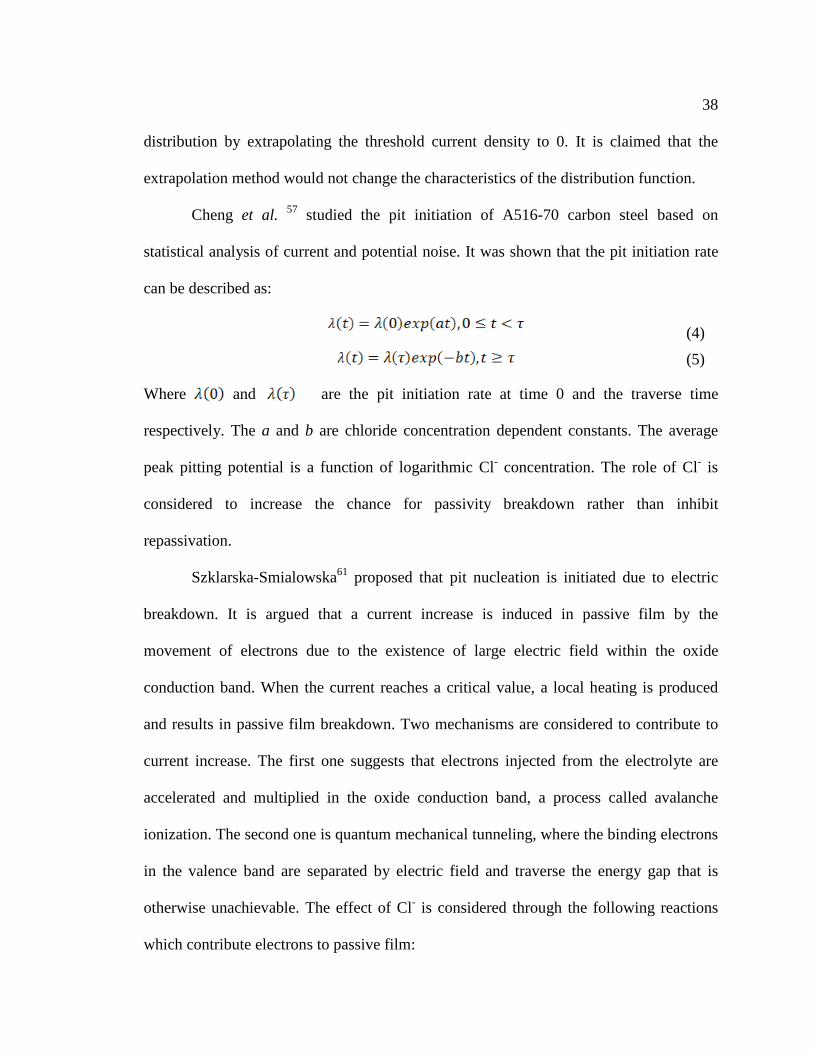
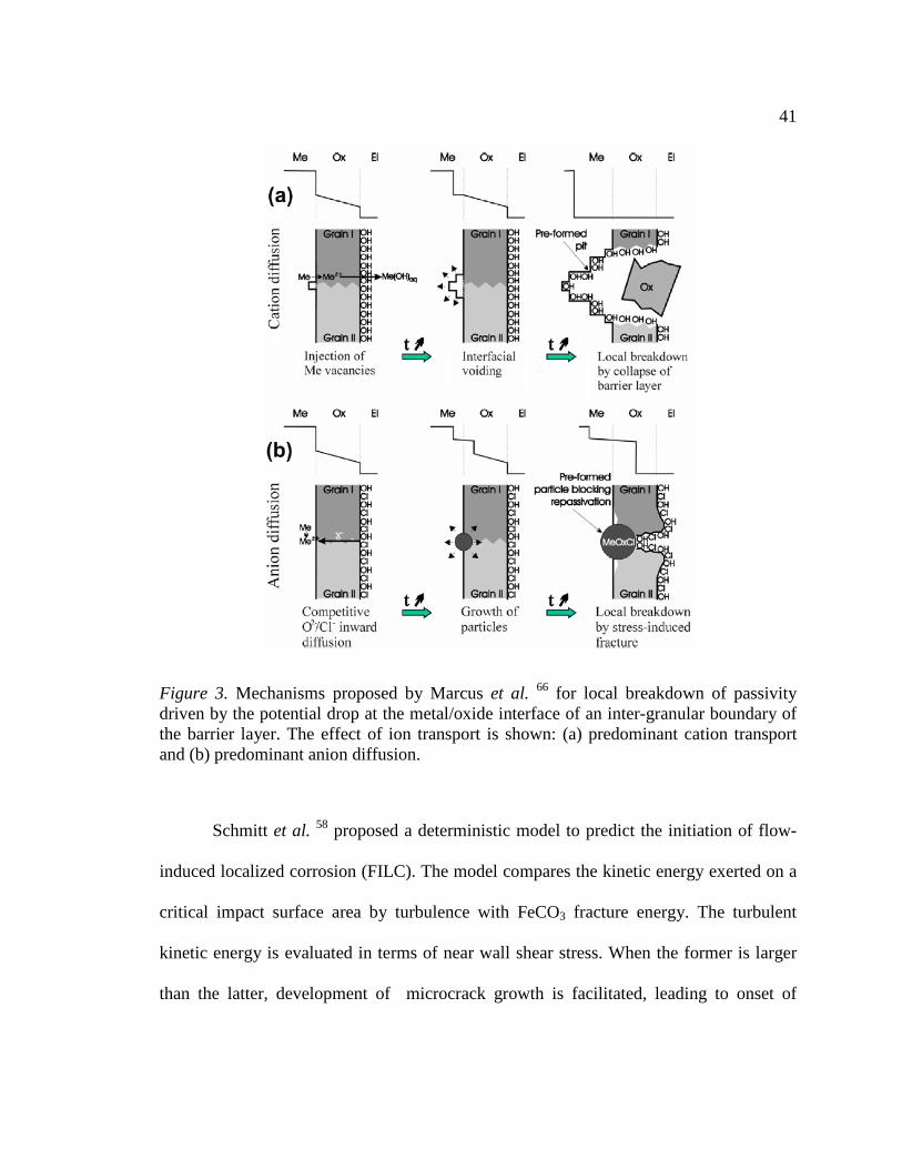
(7) Marcus et al. 66 proposed a model to simulate the passivity breakdown that
predominately occurs on the inter-granular boundaries. The mechanisms considered
include: local thinning and dissolution of oxide film; metal voiding on metal/passive film
interface induced by cation diffusion; and mechanical breakdown by particle growth on
metal/passive film interface induced by anion diffusion. Figure 2 schematically shows the
first mechanism with and without Cl-. Figure 3 demonstrates the second and third
mechanisms respectively. The straight lines on the top of each illustration signify the
potential distribution in the system. Clearly, potential constantly redistributes as the pit
initiation process advances.

40
Figure 2. Mechanism proposed by Marcus et al. 66 for local breakdown of passivity driven by the potential drop at the oxide/electrolyte interface of an inter-granular boundary of the barrier layer. The effect of chlorides is shown.
41
Figure 3. Mechanisms proposed by Marcus et al. 66 for local breakdown of passivity driven by the potential drop at the metal/oxide interface of an inter-granular boundary of the barrier layer. The effect of ion transport is shown: (a) predominant cation transport and (b) predominant anion diffusion.
Schmitt et al. 58 proposed a deterministic model to predict the initiation of flow-
induced localized corrosion (FILC). The model compares the kinetic energy exerted on a
critical impact surface area by turbulence with FeCO3 fracture energy. The turbulent
kinetic energy is evaluated in terms of near wall shear stress. When the former is larger
than the latter, development of microcrack growth is facilitated, leading to onset of

42 FILC. This mechanism is challenged by Yang59, who experimentally showed that the
strength of FeCO3 layer is higher than wall shear stress by several orders of magnitude.
Ergun and Akcay60 investigated the pitting potential of 1018 carbon steel as a
function of pH, chloride concentration and temperature using potentiodyanmic sweep.
The Box-Wilson experiment design concept was adopted in the experiments. By
analyzing a total of 20 experiments, an empirical equation in the form of polynomial
expression was developed, which relates the pitting potential with investigated
parameters. The equation suggests that the interactions between temperature/pH and
pH/Cl- concentration are important factors in determining pitting potential.
Nyborg and Dugstad62 experimentally investigated the mesa attack of carbon steel
in flowing CO2 conditions using in-situ video technique. The initiation of mesa-type
defect is proposed to be related to the competition between corrosion and FeCO3 layer
precipitation for available metal surface. It is argued that when the ratio of the
precipitation rate and the corrosion rate is below a certain level, the void on the metal
surface created by the corrosion process will not be able to be filled by FeCO3
precipitates. The void underneath the FeCO3 layer jeopardizes the mechanical strength of
the film, which can then be removed by hydrodynamic forces. A model developed by
Nešić et al.63 is shown to be able to provide the quantitative information required for
determination of the onset of pit initiation based on the proposed mechanism.
Xiao64 developed a 2D stochastic model to simulate the localized corrosion
process of carbon steel. Uniform corrosion rate and surface scaling tendency were used as
the major inputs for calculation of the probability function, which was originally

43 proposed by Van Hunnik and Pots.65 The model gives reasonable simulation in pit shape;
however, no mechanistic information can be provided by the model due to the lack of
mechanistic background.
From the literature review presented in this section, it can be seen that the
mechanisms of pit initiation are still unclear despite the significant research efforts made
in this area. Various models have been developed based on different proposed
mechanisms, such as electric field, pH, chloride, passive film thickening, flow or a
combination of these factors. A clear pit initiation model cannot be proposed before a
consensus is reached as to the determining factor responsible for pit initiation, and the
deterministic vs. probabilistic nature of pit initiation.
2.3 Pit propagation
Pit propagation is one of the most active research areas in the field of localized
corrosion modelling. Given the corrosive environment favors pit propagation, a pit can
penetrate into the metal at a high rate. The rate of pit propagation directly determines the
service life of pipelines. Most pit propagation models invoke a galvanic coupling
mechanism. In the context of galvanic corrosion, pit propagation rate is dictated by the
potential/current distribution between anode and cathode. Due to the existence of solution
resistance, potential is non-uniformly distributed over the metal surface, leading to varied
anodic dissolution rates on different parts of the anode. Obviously, the solution resistance
effect must be taken into account in pit propagation modelling in order to achieve
reasonable predictions.
44
The earliest mechanistic model for localized corrosion propagation is probably the
one proposed by Pickering and Frankenthal.67 In their work, a 1D model was developed
to simulate the potential and current distribution in a cylinder-shaped pit with passivated
walls and an active pit bottom. In this model, a single electrochemical reaction, metal
oxidation, is considered on the pit bottom. Diffusion and electro-migration are considered
to drive mass transport of metal ions. Chemical equilibrium is assumed in the model. The
simple geometry and simple physics allow them to derive the analytical solutions for
concentration and potential distributions as functions of pit depth. Although this model
over-simplifies the complexity of localized corrosion, the basic principles involved are
widely adopted in the more complicated models developed thereafter.
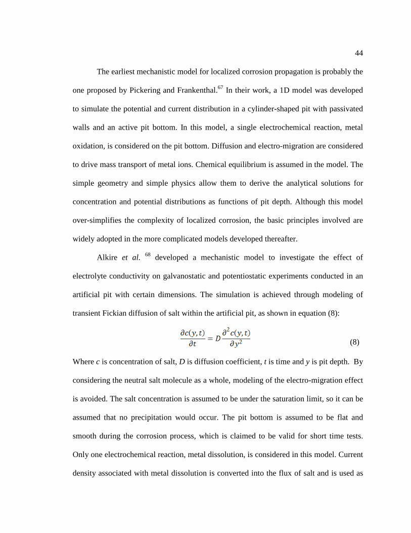
Alkire et al. 68 developed a mechanistic model to investigate the effect of
electrolyte conductivity on galvanostatic and potentiostatic experiments conducted in an
artificial pit with certain dimensions. The simulation is achieved through modeling of
transient Fickian diffusion of salt within the artificial pit, as shown in equation (8):
(8)
Where c is concentration of salt, D is diffusion coefficient, t is time and y is pit depth. By
considering the neutral salt molecule as a whole, modeling of the electro-migration effect
is avoided. The salt concentration is assumed to be under the saturation limit, so it can be
assumed that no precipitation would occur. The pit bottom is assumed to be flat and
smooth during the corrosion process, which is claimed to be valid for short time tests.
Only one electrochemical reaction, metal dissolution, is considered in this model. Current
density associated with metal dissolution is converted into the flux of salt and is used as

45 the boundary condition for the governing mass transport equation. Four components are
considered in calculating the potential between working electrode and reference
electrode: charge transfer resistance, concentration difference resistance, solution
resistance within the pit and solution resistance over the pit mouth.
Alkire and Siitari69 developed a model to simulate current distribution along the
wall of a long narrow pit. In this model, anodic reaction is assumed to occur only at the
pit bottom, while cathodic reaction occurs along the pit wall. Two equations (equation (9)
and (10)) are derived for potential and concentration distributions from Ohm’s law and
Fick’s law, respectively. Metal dissolution and H+ reduction are the only electrochemical
reactions considered, the kinetics of which are assumed to follow Tafel behavior. Mass
transport is attributed only to molecular diffusion, while convective flow is neglected due
to geometric restrictions. The constriction for current flowing into the crevice is
implemented. The model results indicate that cathodic reaction can occur inside the
narrow pit even though the bulk solution contains a low H+ concentration.
( )
−−
= sg
co
s VTRnF
ccai
dxd φαφκ exp02
2
(9)
[ ]
−−
= sg
co V
TRnF
nFccai
dxcdD φαexp02
2
(10)
Where si : current density in the solution; sφ : potential in the solution; κ : solution
conductivity; α : ratio of surface area over volume; 0i : exchange current density; occ, :
local and reference concentration of species; D : diffusion coefficient; cα : transfer
46 coefficient; V: potential of metal; n: electrons involved in electrochemical reactions; F:
Faraday constant; gR : universal gas constant; T: temperature.
Harb and Alkire70 developed a 2D mechanistic model for pitting corrosion of
nickel alloy (Ni) in a stagnant 0.5M NaCl solution at steady-state. Five species are taken
into account in the model (NiCl+, NiCl2, Ni2+, Cl-, Na+). Mass transports of involved
species are simulated for constant applied potentials. In this model, mass transport is
contributed only by molecular diffusion and electro-migration. Chemical equilibrium is
assumed, which gives zero generation or consumption rates of the species. A hemispheric
pit and the solution well beyond the pit are used as the computation domain. The
simulation reveals significant concentration gradients outside the pit indicating the
importance of solution resistance both inside and outside the pit.
Based on the stagnant pitting model, Harb and Alkire71 developed a second model
by including the effect of convective flow. In this model, in-situ velocities are required in
order to solve the mass transport equation. This was achieved by solving the simplified
Navier-Stokes equation (Equation (11) and (12)):
vp 2∇=∇ (11)
0=⋅∇ v (12)
Where v :in-situ velocity; p: pressure.
Galvele72 developed a 1D mechanistic model for pitting corrosion. Two reactions,
metal oxidation and first level metal ion hydrolysis, are considered as the main
mechanism of pitting corrosion, as shown in Equation (13) and (14). In this model,
diffusion is considered to be the only mechanism for species transport, while electro-

47 migration and convection are neglected inside the pit. This is due to the assumption of
sufficient supporting electrolytes in the bulk and lack of convective flow inside the pit
due to geometric restrictions. By solving the mass transport equation (in a similar form
like equation (8)) in conjunction with chemical equilibrium for involved atoms (Me, O
and H), the concentrations of species can be obtained and the fluxes can then be
calculated. An arbitrarily determined constant current is used in the model to give the
flux of metal species. The analytic solution of the equation system leads to the
identification of a key parameter, x.i (product of pit depth and current density), that is
considered to control the occurrence of pitting corrosion. In a later paper, Galvele
published an improved model in which full hydrolysis of cation is taken into account.73
The model generates a relationship between pitting potential and pH. The model suggests
that for a bivalent metal, pitting potential is independent of bulk pH up to the value of 8-9
and becomes pH-dependent at a higher pH; for a trivalent metal, pitting potential is
unaffected by bulk pH due to multiple steps of hydrolysis. Gravano and Gavele74 further
improved the model by taking into account the electro-migration effect. The model was
applied to zinc in a diluted NaCl solution with a borate buffer. The model suggests that
effect of aggressive species (Cl-) on pitting is inhibited by the buffer solution due to
increasing critical x.i value to a level where electro-migration becomes important. In this
case, solution resistance inside the pit plays an important role in determining pitting
potential.
neMeMe n +⇔ + (13)
48
( )( ) +++−+ +⇔++ HOHMeOHOHMe nn 12 22 (14)
Bardal et al. 75 developed a mechanistic model to predict the galvanic corrosion
induced by contact of dissimilar metals. The model is based on the Laplace equation for
potential ( ), solved using the boundary element method, which transforms the
governing equation into the form of:
(15)
Where is the boundary surface of the computational domain. Polarization curves
obtained experimentally for electrochemical reactions are used to describe the boundary
conditions. The variation of cathodic reaction rate at different locations along the metal
surface is estimated by incorporating the concept of diffusion boundary layer
development.
Fu et al. 76 proposed a transient mechanistic model to simulate pit propagation
rate. The model considers the current and potential distribution, mass transport and
hydrolysis of metal ions. The model is initiated by solving for electro-migration potential
and diffusion potential distribution separately, based on initial concentrations and
solution conductivity, as shown in equations (16) and (17), respectively. With the
knowledge of potential distribution, fluxes of species can be calculated using equation
(18). A mass transport equation is then solved to give the concentration distribution in a
new time step (equation (19)). This is followed by an update of solution conductivity and
water chemistry. The process is then repeated for as many time steps as necessary.
49
(16)
(17)
(18)
(19)
Where : current; : solution conductivity; : electromigration potential; : diffusion
potential; : charges of ionic species; : mobility; : concentration; : chemical
potential; : fluxes; : Faraday’s constant and : time.
Benrais and Sohm77 proposed a pit propagation model to simulate pitting
corrosion of aluminum in acidic media. The model is an improved version of the
Pickering67 model. The distribution of concentrations and potentials along the pit depth is
obtained analytically by transforming governing mass transport equations into non-
dimensional form. To derive the analytic expressions for concentration and potential as a
function of pit depth, a number of assumptions are made in the model: the solution inside
the pit is assumed to be dilute; species are assumed to travel through the solution only by
molecular diffusion and electro-migration; aluminum ion is assumed to be saturated on
the bottom of the pit, and no supersaturation is considered. Aluminum ion hydrolysis is
neglected in the model, as is any change of corroding area as a result of corrosion.
Sharland 78,79presented a 2D mechanistic model to simulate the propagation stage
of iron corrosion in crevices and pits with prescribed dimensions. A mass transport

50 equation (equation (20)) is solved for all involved species in conjunction with a charge
balance equation (equation (21)):
( ) iiiiiii RcFuzcDtc
+∇∇+∇=∂∂ φ2 (20)
0=∑ iicz (21)
Where Di : diffusion coefficient of species; ci : concentration of species; zi: electrical
charge number; F: Faraday constant; ui: mobility of species; φ : solution potential; i:
current density; iR :chemical reaction rate; t: time. A few assumptions are made in the
model: passivity is maintained outside the pit/crevice; chemical equilibrium is maintained
for all involved chemical reactions; convective flow is neglected inside the pit/crevice;
dilute solution is assumed; and moving-boundary of pit bottom is slow compared to
migration rate of ions and is therefore neglected. Only one electrochemical reaction, iron
oxidation, is considered in this model. The kinetics of iron oxidation rate are described by
a Tafel expression as a function of potential.
Heppner80 developed a 2D mechanistic model for crevice corrosion. Mass
transport, electrode kinetic, chemical equilibrium and fluid mechanics are taken into
account in his model. The governing equation is:
(22)
Where : concentration of species; : time coordinate; : diffusion coefficient; :
electrical charge number; : mobility of species; : Faraday’s constant; : current
density due to regular potential; : current density due to convection diffusion

51 potential; : in-situ velocity; : solution conductivity; : charge density; : dielectric
constant of water.
Walton et al. 81 presented a mechanistic model to simulate crevice corrosion of
passive and active metals. This model is made in a generic way in order to accommodate
different corrosion systems. The inputs of the model include: specification of species
involved, chemical reactions in the solution, chemical potential of species,
electrochemical reaction kinetics on metal/solution interface and mesh sizes. The model
starts with a calculation of current flowing through the solution based on the current
generated at the metal/solution interface (equation (23)). This is followed by a calculation
of potential distribution using equation (24). Equation (24) suggests that current flow in
the solution is ascribed to electro-migration and diffusion. With the knowledge of
potential and current distribution, mass transport of involved species can then be solved
for using equation (25). It should be noted that the fluxes of electroactive species ( nN )
induced by electrochemical reactions on the metal surface, are directly incorporated into
the governing equation and therefore not used as boundary conditions.
(23)
( )( )
κ
γγγφ
∇+∇+−=∇
∑n
nnnnnnns
s
ccFDzi / (24)
nnc
nn RN
APN
tc
++⋅−∇=∂∂
(25)

52 Where : current density at any point in the crevice corrosion; : current density at the
metal/solution interface; L: the depth of the crevice/pit; : the corroded perimeter (
for a pit, for a crevice); : the position in the crevice measured from the mouth; :
cross-sectional area of the crevice/pit ( for a pit, for a crevice); : solution
potential; : charges of ionic species; : diffusion coefficient; : Faraday’s constant;
: concentration; : activity coefficient; : solution conductivity; : flux of species in
solution; : flux of species on the metal/solution interface; : chemical reaction rate.
Xu et al. 82,83 simulated crevice corrosion based on an IR-driven mechanism. In
their models, potential and current distributions in a crevice are obtained by solving the
Laplace equation for potential. The electrochemical reaction kinetics at the crevice
surface are described by the polarization curve obtained in bulk solution. An iterative
algorithm is used to establish the transition from passive to active surfaces along the
crevice wall. The critical point where transition occurs is shown to be influenced by
polarization behavior of the metal-solution system, solution conductivity, potential at
outside surface of the crevice, dimensions of crevice gap and depth and passive current
density.
Achour et al. developed a mechanistic model for pit propagation of carbon steel in
CO2 environments under turbulent conditions.84 The model takes into account chemical
equilibrium, electrochemical reaction kinetics of iron oxidation, FeCO3 layer formation
kinetics and hydrodynamic conditions inside the pit. In this model, pit
propagation/repassivation is determined based FeCO3 precipitation. Surface Fe2+
concentration is determined by mass balance accounting for chemical reactions, surface
53 electrochemical reactions and mass transfer. The surface Fe2+ concentration is then
compared with the Fe2+ concentration associated with FeCO3 saturation. If the former is
higher than the latter, the pit is considered to be protected; otherwise the propagation rate
is calculated according to Equation (26):
[ ] [ ]( )ssscor FeFekJ ++ −= 22 (26)
Where Jcor : flux of iron dissolution; k: mass transfer coefficient of Fe2+; [ ]ssFe +2 :
saturation concentration of Fe2+ with respect to FeCO3; [ ]sFe +2 : surface Fe2+
concentration.
Engelhardt and Macdonald85 analyzed the relationship between critical pit depth
and critical service life. A quasipotential is proposed in the model as a function of metal
potential. Based on the quasipotenital, they were able to develop the analytical solutions
for potential and concentration distribution inside the pit and the pit propagation rate. The
model shows that the initial anodic current density will not exceed the 10-4-10-3A/cm2
given that the critical pit depth is less than 10mm and that service life is more than 1 year.
This conclusion is limited by the assumption that polarization behavior of anodic
dissolution does not change as a pit propagates. The model also suggests that potential
drop inside the pit can be neglected if the conductivity of the bulk solution is sufficiently
high, roughly in the order of magnitude for seawater. It is claimed that this model can be
used to extrapolate short term experimental results to long term operations.
Laycock et al. 86 proposed a mechanistic model to simulate a pit propagation
process of stainless steel under potentiostatic control. A truncated spherical-shaped pit
and the solution beyond the pit are taken as the computational domain. The pit is assumed

54 to retain the original shape during pit evolution. In this transient model, initial conditions
are set at the point where a pit has just been initiated. At pit initiation, it is assumed that
metallic ions are saturated in the pit, but absent from the outside solution of the pit. A
reference potential of 0V is given everywhere in the domain. Chemical equilibrium is
assumed for reactions inside the pit with the exception of salt precipitation, the rate of
which is proposed to be a linear function of supersaturation. Two electrochemical
reactions, metal oxidation and H+ reduction, are considered in the model. The kinetics of
both reactions are assumed to follow Tafel’s law. The mass transport equation and the
Laplace equation for potential are solved for concentration and potential distribution
under applied potential. The moving boundary due to receding of the pit bottom is
accounted for in the model. Repassivation is considered to occur when anodic current
density exceeds a critical current density defined as a function of dissolved metallic ion
concentration. In a later model, Laycock et al. 87 incorporated a stochastic approach into
the earlier model in order to simulate pit initiation. In this model, 3 geometric parameters
for the pit: radius, degree of opening and depth from the free surface, are specified by a
random function following log-normal distribution. The maximum potential above which
a stable pit is formed and the minimum potential, below which pit dies are empirically
related to three geometric parameters, giving the corresponding fluctuation of potentials.
The number of pit nucleation sites is determined by a binomial function. The Monte-
Carlo simulation is then performed to determine the probability of pit initiation.
Malki and Baroux88 proposed two stochastic approaches to simulate pit growth
kinetics. In the first approach, a fresh metal surface is discretized into multiple sites
55 subject to pitting corrosion. The Monte-Carlo tests are performed with respect to a
dissolution probability, which changes with time. If the test is positive, a pit is developed
with a randomly determined pit radius ranging from 0 to the maximum values determined
by the applied potential and solution corrosivity; the process is then taken to the next time
step. A repassivation probability is also incorporated in the model. At each time step,
iterations are performed as many times as needed to generate a pit. The pit growth rate is
given by the pit depth and the time. In the second approach, the metal/passive
film/electrolyte system is discretized into multiple cells using a technique known as
Cellular Automation. Each site is assigned one of four possible states: corrosion cell,
non-corrosion cell, passive film cell or metallic substrate cell. At each time step, cells can
transform into different states following certain transition rules; the number of corrosion
cells is related to corrosion current. The rules are defined based on the following
assumptions: that a pit is already initiated; that passive film acts as a perfect barrier for
dissolution; and that the corrosion process is under diffusion control.
Scheiner et al. 89 presented a mechanistic model to simulate the stable pitting
growth of stainless steel by assuming a diffusion-controlled corrosion process. Moving
boundaries are taken into consideration in the model. Four computational domains,
namely: solid metal, salt film at pit surface, solution inside and outside the pit, are
identified in the model, where concentrations of metal/metallic ions are calculated in
different ways. The authors accentuated the concentration discontinuity from the salt film
to the pit solution, which incapacitates Fick’s law in calculating concentration gradient
within the salt film. In this model, the evolution of pit shape as a function of time can be

56 mechanistically determined as a result of the corrosion process, which is particularly
related to solid metal concentration, saturation concentration of dissolved metallic ions,
diffusion coefficient of the ions and the boundary ionic flux.
Agarwal et al. 90 developed a model to simulate the current distribution in crevice
corrosion. Potential and current distribution are obtained by solving the Laplace equation
for potential. The effect of non-conductive particulates on the cathode surface is
accounted for by idealizing the particulates into uniform distribution with fixed porosity
and tortuosity. It was argued that the particulates influence current distribution in two
ways: they reduce the electrolyte conductivity due to the effect of volume blockage and
they reduce the electrochemical reaction kinetics by blocking parts of the active surface.
The former is calculated using Bruggeman’s equation91, while the latter is taken into
consideration by involving particulate surface coverage in the surface reaction kinetics.
Han et al. proposed an electrochemical model to calculate the steady-state
localized corrosion rate of carbon steel in CO2 environments.92 The model is based on
their experimental observations which suggest passivation of carbon steel in the presence
of FeCO3. The substance responsible for passivation is proposed to be magnetite (Fe3O4).
Chemical equilibrium is assumed in the model. An experimentally determined passive
current density is used in the model. The cathodic reaction kinetics on the passive surface
are assumed to follow Tafel behavior, and a correction factor is introduced into the
cathodic reaction rate calculation due to the lack of consideration for solution resistance
effect.

57
Amri et al. 93 developed a steady-state model to simulate the pit propagation of
carbon steel in CO2 environments with the presence of acetic acids. A 2D simulation is
performed in a domain containing a pit with prescribed sizes and a diffusion boundary
layer above it. Mass transport equations with consideration of diffusion and electro-
migration are solved for concentration gradient, and the Laplace equation is solved for
potential distribution. The electrochemical reaction kinetics are described by Tafel’s law.
The model shows the depletion of acetic acid and progressive reduction of CO2
concentration towards the pit bottom. This is attributed to the reduction of H+ and
diffusion limitation.
This part of literature review points out two main modeling strategies for
simulating pit propagation in the context of galvanic cell. The first one is solving the
mass transport equation with the electro-migration effect involved, the second one is by
solving the Laplace equation for potential distribution. Essentially, the concept of
electroneutrality is embedded in both approaches. Both methods lead to the potential
distribution along metal surface, which highlights the importance of solution resistance
between electrodes. The consideration of some complicating factors, such as non-
conductive precipitates, changing pit shape, transition of passive-active region along the
pit wall and chemical reactions (such as metal ion hydrolysis), plays a significant role in
determining model complexity and model limitations.

58
CHAPTER 3: RESEARCH OBJECTIVES
The above literature review indicates that most localized corrosion models either
aim at simulating a specific stage of the localized corrosion process or are exclusively
applicable to specific environments, making them less valuable for a carbon steel
exposed to CO2 aqueous system.
The overall goal of this study is to develop a mechanistic model that can be used
to predict the localized CO2 corrosion process of carbon steels. The effect of H2S on
localized corrosion is not known at present and will not be taken into account in this
model. The model is expected to cover the following aspects of the corrosion process:
Uniform or localized CO2 corrosion rate of carbon steel as a function of time;
Concentration profiles of species involved in the corrosion process as functions of
locations and time;
Characteristics of FeCO3 layer formation in terms of porosity and tortuosity as a
function of time;
FeCO3 layer removal on metal surface leading to pit initiation;
Passivation/repassivation effect;
Galvanic effect between anode and cathode.
Potentiodynamic and potentiostatic tests have revealed that the passive film
formed on a carbon steel surface in the system of interest is not as protective as those
present on stainless steel or other alloy surfaces. To make a distinction from commonly-
known passivation as exhibited by alloys, the term “pseudo-passivation” will be used
59 throughout the document to refer to the passive-like behaviour of carbon steel in an
H2O/CO2/Fe2+ environment.
The overall goal of this project was achieved by fulfilling the individual
objectives listed below:
Expand the original CO2 corrosion model of Nešić et al. 13,14 (a “single-point”
model) into a “two-point” model to simulate an anode and cathode of a galvanic
cell and establish the link between the anode and cathode through potential
distribution along the metal surface. This step forms the basis for all future
developments.
Improve the previous FeCO3 layer growth model numerically by solving the
governing equation with a proper higher-order upwind scheme for convection-like
term and the implicit time marching scheme for better stability and faster
calculation;
Investigate the effect of Fe2+ hydrolysis on localized CO2 corrosion of carbon
steel;
Derive the Butler-Volmer expressions for electrochemical reaction kinetics and
implement them into the mass transport equations as implicit boundary conditions
to achieve a realistic potential distribution in a galvanic cell;
Add hydrogen gas as an additional species into the system in order to obtain the
realistic reversible potential of cathodic reactions;
Incorporate thermodynamic calculation for the generation of magnetite to enable
the determination of pseudo-passivation/repassivation;

60 Experimentally determine the major factors affecting pseudo-passive current
density;
Based on the experiments, develop/implement a mechanistic model to calculate
the pseudo-passive current density of carbon steel in CO2 environments;
Investigate the cathodic reaction kinetics on pseudo-passive carbon steel surfaces;
Develop a mechanistic model to obtain the potential and current distribution in a
galvanic cell with the effect of non-conductive FeCO3 layer;
Implement a random function to simulate the stochastic behaviour of pit initiation
in terms of time.
All of the above tasks have been accomplished and are presented in the
corresponding subsections of Chapter 4.

61
CHAPTER 4: MECHANISTIC MODEL OF LOCALIZED CO2 CORROSION
4.1 Introduction
As noted above, localized corrosion presents one of the greatest threats to
integrity of pipelines in oil and gas industry. Extensive research efforts have been made
towards understanding the mechanisms of localized corrosion in the past few decades, yet
the mechanistic understanding of localized corrosion is still limited. This is partly due to
the fact that water chemistry, particularly surface water chemistry, in the restricted area
of a pit is not easily reached by conventional equipment, yet it often differs substantially
from the bulk solution. The picture is further complicated by the fact that initiation of
pitting corrosion is difficult to manage and detect, even in highly controllable laboratory
experiments. Pit initiation often manifests itself as a seemingly random process as to
when and where it occurs. This has led to a number of stochastic models for pit initiation,
as discussed in Chapter 2. One can intuitively imagine that localized corrosion has to do
with water chemistry in close proximity to the metal surface, but this is not yet fully
understood by the corrosion community. Therefore, it would be beneficial to determine
the physic-chemical parameters near the steel surface, such as water chemistry and
electrochemical properties, in order to understand the process of localized corrosion.
Unfortunately, up to now, no experimental methods are reliable for detecting localized
corrosion or local water chemistry, making it one of the biggest challenges for corrosion
research. Due to the difficulties associated with experimental means, a mechanistic model
can be helpful towards the understanding of localized corrosion of carbon steel.
62
The goal of this chapter is to present a transient mechanistic model that can be
used to predict the details of the corrosion process of mild steel exposed to an aqueous
environment containing CO2. It should be mentioned that localized corrosion can be
governed by multiple mechanisms, as can be seen from the review of the various
localized corrosion models presented in Chapter 2, such as pit acidification, concentration
differentiation cells and flow induced corrosion, to name a few. This model is designed to
cover one of the major mechanisms for localized corrosion of mild steel in CO2
environments: galvanic coupling between the bare pit (anode) and the pseudo-passive
surface (cathode), and is primarily based on the recent studies at the ICMT.11 The model
is built based upon fundamental theories governing chemistry, electrochemistry and
transport phenomena. Evolution of the corrosion process is simulated as a function of
time. Depending on specific physical and chemical conditions, uniform or localized
corrosion might be predicted. After a randomized event is triggered for the initiation step
of localized corrosion, the model can predict and simulate the transition from uniform to
localized corrosion according to appropriate theories. Various factors involved in the
corrosion processes, such as FeCO3 layer precipitation and dissolution, solution
resistance, pseudo-passivation, depassivation and repassivation are built into the model to
give a comprehensive and physically realistic description of the actual process. In
addition to the corrosion rate, the model also provides other valuable information to help
evaluate environment corrosivity and explain corrosion behavior. This information
includes: electrochemical potential distribution, current distribution, concentrations of
species, fluxes of species, and FeCO3 layer properties at any given location and time.

63
In the following subsections, the processes simulated in the model are
qualitatively described, followed by theories governing various phenomena and
mathematical descriptions of the theories. Model verification and parametric study are
then presented to discuss how key parameters affect the localized corrosion process. The
assumptions and limitations of the model are then presented in final portion of the
chapter.
4.2 Physico-chemical Processes Described by the Model
The model describes CO2 localized corrosion process in terms of three stages:
pseudo-passivation/ repassivation, pit initiation and pit propagation. Each of these stages
has its unique mechanisms and characteristics, and therefore each has to be considered
separately. The processes simulated in this model are described below.
When carbon steel is in contact with an aqueous CO2 solution, electrochemical
reactions occur on the steel surface. Some species are consumed and others are generated,
which establishes the concentration gradients of the species. As the corrosion process
proceeds, ferrous ion (Fe2+) is continuously released into the solution and varies the water
chemistry. When the product of the concentrations for Fe2+ and CO32- in the solution
exceeds the solubility limit of FeCO3, it will precipitate out of the solution and build a
layer on the metal surface. This deposited corrosion product poses significant mass
transfer resistance to species (including H+) moving to/ from the bulk solution which
leads to an increased pH at the metal surface. The pH increase enables the formation of a
pseudo-passive phase beneath the corrosion product layer, which is thought to be a
mixture of FeCO3, Fe(OH)2 and/or Fe3O4. As a result of pseudo-passivation, the metal

64 potential increases. Evidently, up to this point in the scenario, the metal experiences
uniform corrosion. It can be assumed that at some point in time, a small area of the metal
loses its protective film, leading to depassivation and resulting in potential drop within
this area. Therefore, a potential difference is established between this small film-free
active surface (which has now become an anode) and the large film-covered pseudo-
passive surface around the anode (which has now become a cathode). Based on the
galvanic coupling mechanism, this potential difference can drive the anode to corrode at a
much higher rate than which would be experienced with uniform corrosion. In cases
where supersaturation of FeCO3 in the solution is sufficiently high, substantial amounts
of Fe2+ resulting from pit propagation promote further precipitation of FeCO3 on the
anode. This may again increase the surface pH of the anode and facilitate repassivation,
which would lead to pit death. The processes described above are schematically
illustrated in Figure 4 through Figure 9 .

65
Figure 4. Illustration of corrosion process: FeCO3
layer formation leading to surface pH increases.
Figure 5. Illustration of corrosion process: pseudo-passivation leading to potential increases.

66
Figure 6. Illustration of corrosion process: depassivation leading to separation of anode and cathode and establishment of potential difference.
Figure 7. Illustration of corrosion process: Pit propagation.

67
Figure 8. Illustration of corrosion process: FeCO3 re-precipitation if superstaturation of FeCO3
is sufficiently high.
Figure 9. Illustration of corrosion process: Repassivation leading to pit death.

68 4.3 Physico-chemical Model
Localized CO2 corrosion is a complex process that involves multiple physic-
chemical processes, dependent on each other. These include: chemical reactions,
electrochemical reactions, mass transport, FeCO3 layer formation, pseudo-
passivation/repassivation, pit initiation and pit propagation. These factors must be taken
into account in the model in order to provide a realistic description of the corrosion
process.
4.3.1 Chemical Reactions
Gaseous CO2 and water are almost always present in various quantities along with
oil and gas in pipelines. Various chemical reactions take place in the water phase due to
the presence of CO2. These reactions have to be taken into consideration in order to
obtain accurate concentration profiles of corrosive species for further calculation.
It is generally agreed that most chemical reactions proceed much faster than other
processes involved in corrosion, such as mass transport and electrochemical reactions.
Therefore, many corrosion models neglect the chemical reaction effect by assuming the
preservation of chemical equilibrium in the solution. This assumption does not apply in a
CO2 corrosion environment, since CO2 hydration, (Reaction (28)), has been reported to
be a slow step94 and in some cases becomes a rate-limiting step in the CO2 corrosion
process. Hence, a local non-equilibrium condition is likely to exist, which alters the
corrosion process.
For a CO2 aqueous system, the following reactions are considered to be present at
all times:

69
)(2)(2 aqg COCO ⇔ (27)
( ) ( ) ( )aqaqaq COHOHCO 3222 ⇔+ (28)
( ) ( ) ( )aqaqaq HCOHCOH −+ +⇔ 332 (29)
( ) ( ) ( )aqaqaq COHHCO −+− +⇔ 233 (30)
( ) ( ) ( )aqaqaq OHHOH −+ +⇔2 (31)
In some environments, organic acids, particularly low-molecular-weight organic
acids, are found primarily in the water phase and can lead to corrosion of mild steel as
well. Acetic acid (CH3COOH or in shorthand: HAc), the most prevalent type of organic
acid found in brines, can be treated as the representative of all other types of organic
acids, as similar corrosiveness has been established for all types of low-molecular-weight
organic acids.95 The HAc partially dissociates in the water phase to release H+ and Ac- ,
as indicated by Reaction (32). It is stronger than H2CO3, and therefore serves as the main
source of H+ when similar concentration of the two acids are encountered.
( ) ( ) ( )aqaqaq AcHHAc −+ +⇔ (32)
Another chemical reaction that plays a vital role in CO2 corrosion is FeCO3
precipitation (Reaction (33)). Precipitation proceeds when the product of concentrations
of Fe2+ and CO32- in aqueous phase exceeds the solubility limit of FeCO3. Unlike other
chemical reactions occurring homogeneously in the solution, FeCO3 precipitation is a
heterogeneous process. Nucleation of solid iron carbonate occurs preferentially on the
steel surface or inside the void space within the present solid layer.13 This reaction will be
discussed further in section 4.3.4.

70
( ) ( ) ( )saqaq FeCOCOFe 323
2 ⇔+ −+ (33)
For a localized corrosion process, another reaction that merits discussion is Fe2+
hydrolysis, shown in Reaction (34). As noted in the literature review, some localized
corrosion models are built based on a pit acidification mechanism resulting from metallic
ion hydrolysis, particularly in oxygen-containing environments. One aim of this study is
to clarify the role of Fe2+ hydrolysis in the localized CO2 corrosion process in terms of pit
acidification. If significant H+ enrichment is caused by this reaction, it must be taken into
consideration in the model.
++ +↓⇔+ HOHFeOHFe 2)(2 222 (34)
In this work, theoretical calculations are performed based on thermodynamic
theory in order to evaluate the significance of Fe2+ hydrolysis reaction in oxygen-free
CO2 environments.
At equilibrium, the equilibrium constant of a reaction can be related to Gibbs free
energy in the following fashion:
omr
o GKRT ∆−=ln (35)
where R is universal gas constant; T is absolute temperature; Ko is equilibrium constant
for the standard condition and omG is standard Gibbs free energy of a reaction.
Gibbs free energy of a reaction is given by the chemical potentials of species
involved in the reaction as:
∑=∆ oii
omrG µν (36)

71 where iν is the stoichiometric coefficient of species in the reaction and o
iµ is the
standard chemical potential of species.
The combination of Equations (35) and (36) yields:
RTK
oBBo ∑−= µν
ln (37)
For Fe2+ hydrolysis at 25ºC, the equilibrium constant can be obtained by
substituting corresponding standard chemical potentials into Equation (37) , which yields:
29.13log −=oK (38)
The equilibrium constant of Reaction (34) can be given as:
(39)
Where and are concentrations of H+ and Fe2+ respectively.
Combination of Equations (38) and (39) yields:
(40)
Equation (40) allows the calculation of equilibrium pH produced by hydrolysis
reaction of Fe2+ at 25°C. For a saturated solution of FeCl2 in which Fe2+concentration is
around (8 mol/L), Equation (40) yields a pH of 6.2; for concentration of
Fe2+ at 50ppm, which is commonly considered to be a high concentration in oil fields, the
equilibrium pH is around 8.2. Clearly, hydrolysis of Fe2+ would not lead to substantial
solution acidification in a typical CO2 aqueous environment. Therefore, this reaction can
be neglected in the bulk solution as the additional source of H+. However, it should be
noted that on the corroding metal surface particularly underneath the FeCO3 layer where
72 pH increase and Fe2+ enrichment are expected, the equilibrium pH of Reaction (34) could
be achieved to trigger Fe2+ hydrolysis. In fact, Fe2+ hydrolysis is proposed in this model
to be an essential step to promote pseudo-passivation of carbon steel in CO2
environments.
4.3.2 Electrochemical reactions
For CO2 corrosion, several electrochemical reactions are considered to contribute
to the overall corrosion rate of mild steel.
4.3.2.1 Anodic reactions
Dissolution of iron is the dominant anodic reaction. This reaction proceeds via a
multi-step mechanism that is mildly affected by pH and CO2 concentration.13 Within the
range of typical CO2 corrosion, e.g. 4<pH<6, the dependency on pH tends to diminish.13
Therefore, the dependence of the anodic dissolution rate on pH and CO2 is neglected in
the model. At the corrosion potential (and up to 200 mV above), this reaction is under
charge transfer control and the electrochemical behavior can be described using the
Butler-Volmer equation as presented in Table 2.
eFeFe 22 +→ + (41)
4.3.2.2 Cathodic reactions
H+ reduction is one of the main cathodic reactions:
222 HeH →+ −+ (42)
This reaction is limited by how fast H+ can be transported from the bulk solution
to the steel surface through the mass transfer layer (including the liquid boundary layer

73 and the FeCO3(s) layer if it exists). Higher corrosion rates are observed for a CO2
aqueous solution compared to strong acid solutions (such as HCl) at the same pH.
However, for a practical CO2 system where 4<pH<6, the limiting current of this reaction
would be small due to the relatively low concentration of H+. This suggests that CO2 also
plays a certain role in H+ reduction. This can be explained by the fact that the
homogeneous dissociation of H2CO3 provides an additional reservoir for H+ ions, which
then absorbs on the steel surface and gets reduced according to Reaction (42).
Apparently, any rapid consumption of H+ can readily be replenished by Reactions (29)
and (30). Thus for typical CO2 corrosion, the presence of CO2 leads to a much higher
corrosion rate than would be found in a strong acid solution with the same pH.
In the vicinity of the steel surface, another electrochemical reaction can take place
as well: H2CO3 adsorbs at the steel surface and is directly reduced according to Reaction
(43). This is referred to as “direct reduction of carbonic acid”.94 As argued by Nešić et
al. 13, this reaction is just an alternative pathway for the same cathodic reaction -
hydrogen evolution because addition of Reactions (29) and (42) leads to Reaction (43).
The distinction is only in the pathway, i.e in the sequence of reactions.
−− +→+ 3232 222 HCOHeCOH (43)
The rate of this additional hydrogen evolution reaction due to the presence of CO2
is mainly controlled by the slow CO2 hydration step (28) and is a strong function of
H2CO3 concentration which directly depends on partial pressure of CO2.
Acetic acid is known to be one of the species that attacks mild steel. Studies have
shown that it is the undissociated (“free”) HAc and not the acetate ion Ac- that is
74 responsible for corrosion.96 The presence of organic acids is a major corrosion concern,
particularly at lower pH and high temperature as more HAc would be generated under
these conditions according to Reaction (32).
Like H2CO3, HAc provides an additional source of H+, which then adsorbs at the
steel surface and reduces according to the cathodic reaction (42).96 Following the same
reasoning as with H2CO3, it is also possible that the HAc molecule itself is adsorbed at
the steel surface and gets reduced,97 which is often referred to as the “direct HAc
reduction” pathway:
−− +→+ COOCHHeCOOHCH 323 222 (44)
Another possible pathway for hydrogen evolution is the direct reduction of water:
−− +→+ OHHeOH 222 22 (45)
Compared to the cathodic reactions described above, this pathway is very slow
and can often be neglected in practical CO2 corrosion environments. It has been argued
that this reaction becomes significant only under very specific conditions, such as those
encountered in very low partial pressure of CO2 (PCO2 << 0.1 bar) and high pH (pH
>6),13 which is not common in oil and gas pipelines. Hence, this reaction is neglected in
the model.
Bicarbonate reduction, as shown in Equation (46), has spurred extensive debate as
to its significance to the overall corrosion process. Some people argue that this reaction,
although much slower than the direct reduction of H2CO3, could happen above a critical
pH (around 8) at which H2CO3 would be depleted due to insufficient supply from the
bulk. This would be due to the slow formation rate of H2CO3, and HCO3- becoming the

75 dominating species underneath the film. Other people considered the kinetics of this
reaction to be sufficiently low that, no matter how much HCO3- exists underneath the
film, it would not be able to contribute to the overall corrosion rate significantly.
However, it can be argued for a typical CO2 environment where bulk pH ranges from 4 to
6 that this reaction is unlikely to change the corrosion rate in an appreciable fashion. For
practical purposes (this reactions is difficult to distinguish experimentally and hence
theoretically from direct carbonic acid reduction), it is neglected in the model.
−−− +→+ 2323 222 COHeHCO
(46)
4.3.3 Mass transport
Mass transport is an important part of the corrosion process since it strongly
interacts with electrochemical reactions on the steel surface. Due to electrochemical
reactions, certain species are produced or consumed on the steel surface. The mass
transport process sweeps away or replenishes corresponding species changing their
surface concentration what alters electrochemical reaction kinetics. Compared to some
fast electrochemical reactions, such as H+ reduction (42), mass transfer of H+ proceeds
much more slowly; therefore, the rate of the overall reaction is likely to be limited by the
transport process, i.e. how fast this species can move through the mass transfer boundary
layer and porous FeCO3 layer. It is therefore essential to incorporate mass transport rates
into the model in order to obtain an accurate depiction of the overall corrosion process.
Mass transport of species is mainly affected by three mechanisms: molecular
diffusion, electro-migration and convection. Molecular diffusion is essentially a result of
the Brownian motion of species, which manifests itself as an oriented movement along a

76 concentration gradient. For example when species are preferentially consumed on a steel
surface, the amount of species moving towards the steel surface would be greater than
those moving in the opposite direction. From the macroscopic perspective, it would
appear that species move in a direction towards the steel surface. By the same token, for
species generated on the steel surface, the net effect would be to drive species away from
the steel surface.
Electro-migration is caused by the potential gradient established by species with
different diffusion speeds. It acts only on charged species by electrostatic attraction
force. In an aqueous solution, some species diffuse faster while others lag behind. For
example, H+ usually travels much faster than other species. Due to the positive charge of
H+, a potential field is established between fast-moving H+ and other species with
negative charges, which tend to fall behind. This potential field accelerates the movement
of negatively-charged species and slows down fast-moving species with positive charges,
such as H+. It should be noted that, although electro-migration acts only on the charged
species, it is able to exert a certain impact on non-charged species by changing the
chemical reaction rate. For spontaneous uniform corrosion where no external potential
field is applied in the solution, the electro-migration effect is usually negligible, since any
potential difference established due to variation of diffusion can easily be annihilated by
large amounts of supporting electrolytes, such as in a NaCl solution. The simulations
using the previous version of the MULTICORP model,13 a mechanistic uniform corrosion
model (on which the present model is based), have shown that the contribution of electro-
migration to overall fluxes of species is small and can be neglected in spontaneous

77 uniform corrosion. However, when dealing with localized corrosion, a notable potential
difference exists between anode and cathode, which affects the electro-migration;
therefore, the effect of electro-migration must be accounted for in a localized corrosion
scenario.
Convection is the movement of species carried by bulk flow. The convective flow
in the direction parallel to the steel surface does not directly contribute to the corrosion
process, while that in the direction perpendicular to steel surface contributes due to the
mass transport of species. As turbulent eddies penetrate deep into the diffusion layer they
shorten the distance over which diffusion and electro-migration take over. It should be
stressed that no turbulence can exist in close proximity to the steel surface; species can
travel through this region solely by molecular diffusion and electro-migration. In
addition, the effect of convection becomes negligible when a porous FeCO3 layer is
present on the steel surface, forming a major diffusion barrier. This is discussed under the
following heading.
4.3.4 FeCO3 precipitation
The FeCO3 layer, once formed, often controls the rate of corrosion due to
substantial mass transfer resistance within the tortuous path of the film. It is well known
that the protectiveness of the FeCO3 layer is a function of corrosion rate and precipitation
rate, which can be quantified by the so-called “scaling factor” as shown in (47):98
(47)
Where is the scaling factor, is the precipitation rate and CR is the corrosion
rate, expressed in the same units. With a scaling factor greater than a critical value (which
78 means precipitation proceeds faster than corrosion), the FeCO3 layer is dense and
protective; for a scaling factor less than the critical value (which means precipitation is
slower than corrosion), FeCO3 becomes porous and non-protective. Apparently, the
protectiveness of FeCO3 is determined by the competing effects of corrosion and
precipitation.
For localized CO2 corrosion, FeCO3 affects the corrosion process in four distinct
ways. First, as FeCO3 is formed by precipitation, it acts as the sink for Fe2+ and CO32-
ions by reducing their concentrations in the solution, which leads to local acidification of
the solution according to Reaction (30). Second, the tortuous path within the
discontinuous FeCO3 layer poses a significant mass transfer resistance to species moving
towards or away from the metal surface and slows down the electrochemical reactions.
Third, the presence of non-conductive FeCO3 layer on the metal surface effectively
reduces the surface area exposed to the corrosive environment by covering up parts of the
surface, which effectively slows down the electrochemical reactions. Lastly, the
conductivity of the solution is reduced with the presence of the FeCO3 layer by reducing
cross-section areas through which conductive species can travel. It is worth mentioning
that the effect of FeCO3 on solution conductivity is negligible in a uniform corrosion
process, as solution resistance does not play a significant role due to the close proximity
of anode and cathode on the steel surface.
4.3.5 Pseudo-passivation
Research carried out in the past few years11 has revealed that, when FeCO3 layer
forms, carbon steel exhibits a remarkable increase in potential, suggesting the occurrence

79 of pseudo-passivation on the steel surface. Steel surface analysis has confirmed the
existence of magnetite (Fe3O4) and/or Fe(OH)2,12 species commonly known to be related
to passivity.
Pseudo-passivation of carbon steel in CO2 environments allows for possible
occurrence of localized corrosion as it can substantially raise the potential of the metal
substrate and create a potential difference once depassivation occurs in localized areas.
In the present model, the pseudeo-passive film formation is related to formation of
magnetite, which forms via a two-step process as shown by Reactions (48) and (49). In
this process, Fe(OH)2 is first formed by Fe2+ hydrolysis, which is followed by oxidation
of Fe(OH)2 to form magnetite.
(48)
(49)
The occurrence of pseudo-passivation can be illustrated in the context of the
Pourbaix diagram. Figure 10 shows a Pourbaix diagram for a Fe/CO2/H2O system for
80°C, 1ppm Fe2+. Lines 1 and 2 correspond to Reactions (48) and (49), respectively.
Under typical CO2 environments, the operating point usually falls into the area of Fe2+,
indicating an active corrosion process (left of Line 1). At higher pH the solution is
favoring FeCO3 precipitation (right of Line 1), and in that case the surface pH will
spontaneously increase beyond the bulk value as the FeCO3 layer continues to form and
present a mass transfer barrier. At some stage the operating point at the steel surface
could reach Line 2 and magnetite would form, what is in the current model considered to
be the required condition for occurrence of pseudo-passivation.

80
Figure 10. The Pourbaix diagram for Fe/CO2/H2O system with temperature 80°C, [Fe2+
]1ppm. Courtesy of T. Tanupabrungsun.
It should be noted that in this model, occurrence of pseudo-passivation is assumed
to be very fast i.e. once the conditions for magnetite formation are reached it forms
immediately, i.e. the kinetics associated with the formation of pseudo-passive film can be
neglected.
4.3.6 Depassivation and pit initiation
Pit initiation is caused by depassivation i.e. a loss of protective layers (FeCO3
layer and the pseudo-passive film) on certain parts of the steel surface leading to bare
steel being exposed. This process often exhibits a large extent of scatter with regard to the
time and the location. Without a clear understanding of the mechanism, this seemingly
random phenomenon is often simulated using statistical approach.
1 2
81
The mechanism of pit initiation of carbon steel in CO2 environment is an ongoing
topic of research at ICMT. Initial inquiry seems to suggest that chemical dissolution of
FeCO3 is the most important factor leading to depassivation. At this stage, the
mechanisms involved in film removal are not completely understood so in the current
model, the worst case scenario is assumed and the FeCO3 layer is “artificially” removed
some time after pseudo-passivation is achieved. This provides an active anode area and a
galvanic cell is established, which could be stable – leading to pit propagation or
repassivation could occur leading to pit death.
4.3.7 Repassivation and pit death
Repassivation is a process in which an active steel surface may regain passivity
under proper conditions, leading to an arrest in pit growth or so called pit “death”. In a
CO2 environment, repassivation of carbon steel occurs when solution supersaturation
with respect to FeCO3 becomes sufficiently high, which triggers fast precipitation of
FeCO3 on the anode. This would raise the surface pH to a level at which pseudo-passive
film formation is favorable. In addition, increased Fe2+ concentration from the corrosion
process also helps to drop the critical pH required for the formation of Fe(OH)2. As can
be seen in Reaction (48), increased Fe2+ favors the formation of Fe(OH)2. In this model,
onset of repassivation is determined by the same thermodynamic criterion as used for
pseudo-passivation. This is to say that, once thermodynamic conditions are reached for
the formation of magnetite through Reactions (48) and (49), repassivation is assumed to
occur immediately.

82
4.3.8 Pit propagation
For carbon steel corroding in a CO2 environment, the galvanic coupling
mechanism was found to govern pit propagation.11 This theory suggests that once local
depassivation takes place on a small area of the steel surface, a potential difference is
established between this active surface (anode) and the pseudo-passive surface around it
(cathode). Such a potential difference serves as the driving force allowing the pit to
propagate. In this process, the cathodic current occurring on the large area of the cathode
is balanced by the anodic current on the small area of the anode, leading to a substantial
anodic dissolution rate of the steel.
However, it has been found that the potential difference between anode and
cathode alone would generate an unrealistically high pit propagation rate (100 mm/y or
higher) which is not observed under realistic conditions. This can be explained by the IR
potential drop mechanism proposed by Pickering et al. to account for the solution
resistance between electrodes.82,83 In a uniform corrosion scenario, anode and cathode
are so close to each other that solution resistance does not play a significant role as long
as supporting electrolytes are present. However, in the case of localized corrosion, anode
and cathode are separated leading to appreciable solution resistance between them. This
solution resistance can sometimes limit the anodic dissolution rate to a large degree.
Depending on how far the anode is from the cathode, the pit propagation rate would be
different on different parts of anode surface, as solution resistance varies with the
distance between electrodes. Figure 11 schematically shows the potential and current
variation in a galvanic cell. It is important to note that electrochemical reactions are

83 driven by the electrode potential, which is defined as the potential difference across the
double layer:
(50)
where E is electrode potential driving electrochemical reactions; is the unique
potential of the metal and is the potential drop across the double layer.
As shown in Figure 11, a potential distribution exists along the metal surface
with higher potential on the cathode and lower potential on the anode. The potential
difference becomes larger as anode and cathode are separated further away from each
other due to higher solution resistance. This potential distribution results in non-
uniformly distributed current along the metal surface. Clearly, neglecting the effect of
solution resistance would lead to over-prediction of the pitting corrosion rate.

84
Figure 11. Illustration of potential distribution in a galvanic cell. represents the
solution potential drop across the double layer, represents the electrode potential at
different locations, represents metal potential.
4.4 Mathematical Model
The theories described in section 4.3 can be mathematically described by
corresponding physico-chemical laws. The mechanism involved in pit initiation is not
presently available. In this model, the occurrence of pit initiation is triggered simply by
removing protective layers on a small area of the steel surface (anode) at a randomly
determined point in time.
4.4.1 Chemical reactions
Various chemical reactions occur simultaneously in a CO2 /H2O/carbon steel
system. The major chemical reactions are shown in Reactions (27) through (31). As
mentioned earlier, chemical equilibrium does not always exist in CO2 corrosion systems
as CO2 hydration is a slow process, and the generation rate of H2CO3 by Reaction (28)
might lag behind the consumption rate of H2CO3 on the steel surface, creating local non-
equilibrium conditions, especially near the steel surface. To give a realistic description of
the corrosion process, this model calculates the kinetics, i.e. the actual consumption or
generation rate of a species through homogenous chemical reactions, without imposing
chemical equilibrium. In cases where chemical reaction (both consumption and
generation rates of species) are much higher than other processes (transport and
electrochemical reactions), the species concentration is virtually unaffected by other
85 processes and therefore maintained at equilibrium; on the other hand, if the chemical
reaction rates are slow (such as CO2 hydration), the concentration of the involved species
is influenced by other processes, which could then lead to non-equilibrium
concentrations.
The complexity of mathematically modeling the CO2 corrosion processes is
largely due to the presence of chemical reactions by which various species concentrations
are coupled, making the governing equations for mass transports strongly coupled and
highly non-linear. The chemical reaction rate pertaining to any given species is calculated
as the net consumption/generation rate. For a CO2 aqueous system, it has been already
shown that the following reactions are present:
)(2)(2 aqg COCO ⇔ (51)
( ) ( ) ( )aq
k
kaqaq COHOHCO
hyf
hyb
3222
,
,
⇔+ (52)
( ) ( ) ( )aqaq
k
kaq HCOHCOHcaf
cab
−+ +⇔ 332
,
, (53)
( ) ( ) ( )aqaq
k
kaq COHHCO
bif
bib
−+− +⇔ 233
,
, (54)
( ) ( ) ( )aqaq
k
kaq OHHOHwaf
wab
−+ +⇔,
,2
(55)
Reaction (51) is always at equilibrium in CO2-containing pipelines due to
unlimited supply of CO2 in the gas phase. The net reaction rates of Reactions (52)
through (55) can be expressed as the difference between forward and backward reaction
rates:

86
(56)
(57)
(58)
(59)
Based on the law of mass conservation, for a specific reaction, the mass
consumed must be balanced by that generated. The consumption/generation rate of
involved species due to Reactions (52) through (55) can be respectively expressed as:
(60)
(61)
(62)
(63)
Combining the equations above, the net reaction rate of various species can be
calculated as:
(64)
(65)
(66)
(67)
(68)
(69)

87
Equations (64) through (69) present a lengthy and rigid method for calculating the
net reaction rate. Nešić et al. 13 proposed a convenient way to group reaction rates
together in the form of:
(70)
Where is the chemical reaction rate of the jth species; is the stoichiometric
coefficient matrix with j being the number of rows in the matrix for the jth specie and k
being the number of columns in the matrix for the kth reaction; is the net reaction rate
of the kth reaction.
Using equation (70) on a CO2 system, the chemical reaction rates of species can
be expressed as:
(71)
Where the vector on the left side of the equation represents the net chemical reaction
rates of various species, the first term on the right side of the equation is the tensor
(representing the stoichiometric coefficient of each species in various chemical reactions,
with negative values being reactants and positive values being products), and the second
term on the right side of the equation is the vector for net reaction rate of the individual
reaction (the value of which is related to concentrations of species, as shown in Equations
(56) through (59)). The rate constants used in the model were compiled by Nešić et al.
and can be found in the open literature.13

88
With this technique, additional chemical reactions (such as HAc dissociation, H2S
dissociation and HS- dissociation) can easily be incorporated into the model without
increasing numerical difficulty.
The above technique can efficiently handle homogeneous chemical reactions in
the bulk solution. However, for heterogeneous reactions, such as FeCO3 formation and
dissolution that occur only on existing solid surfaces, special consideration is required.
The FeCO3 precipitation and dissolution act as the sink and source for Fe2+ and CO32-
respectively. When supersaturation is greater than 1, net FeCO3 precipitation occurs
which consumes Fe2+ and CO32-; when it is less than 1, net FeCO3 dissolution takes place
leading to increased concentrations of Fe2+ and CO32-.
For the precipitation process, the rates of consumption of species read:
(72)
For the dissolution process, the rates of generation of species can be obtained by:
(73)
The precipitation rate of FeCO3 is given by Sun as:99
(74)
Where is the precipitation rate in mol/m3.s; A and B are constants taking the values
of 28.2 and 64.85 respectively; is the surface volume ratio of the FeCO3 in 1/m; is
the solubility limit of FeCO3 in (mol/L)2, which can be obtained by:99
(75)

89 Where I is the ionic strength in mol/L and T is the temperature in K; is the
supersaturation of FeCO3 defined as:
(76)
The dissolution rate of FeCO3 is developed based on the assumption that the
dissolution process is always under mass transfer control. This assumption is deemed
valid considering that dissolution rate is usually much faster than precipitation rate (5
folds higher or more).100 This assumption implies saturation of FeCO3 at a dissolving
FeCO3 surface (SS=1), since fast dissolution would cause accumulation of Fe2+ and CO32-
on the surface; the extent of accumulation, however, cannot exceed the solubility limit of
FeCO3, otherwise, FeCO3 precipitation would occur. This assumption allows the
derivation of the equation for FeCO3 layer dissolution kinetics as shown by Equation
(77). The equation was derived by Lee101 and detailed equation derivation is shown in
Appendix 1 for reference.
(77)
Where is the dissolution rate of FeCO3 in mol/m3.s; is the time interval in
seconds over which dissolution occurs.
4.4.2 Electrochemical reactions
Electrochemical reactions considered in this model include:
eFeFe 22 +→ + (78)
222 HeH →+ −+ (79)

90
−− +→+ 3232 222 HCOHeCOH (80)
−− +→+ COOCHHeCOOHCH 323 222 (81)
Electrochemical reactions are heterogeneous reactions that take place only on
conductive surfaces (such as a metal surface) in a spontaneous corrosion process. The
reaction rates are a function of surface water chemistry and potential. Due to the
involvement of electrochemical potential, the reaction rate of an electrochemical reaction
is commonly expressed in terms of current density, rather than flux as in a chemical
reaction. In a carbon steel localized corrosion scenario, both an active surface (anode)
and a pseudo-passive surface (cathode) are present. The different nature of these steel
surfaces can lead to significant differences in electrochemical reaction kinetics.
Therefore, efforts were made in this work to identify the difference in electrochemical
reaction kinetics on active and pseudo-passive surfaces and to develop models to
calculate the reaction kinetics on different surfaces.
4.4.2.1 Active surface
In the previously developed uniform corrosion model (MULTICORP V4), the
Tafel equation is used to calculate the current densities of electrochemical reactions,13 as
shown in Equation (82):
(82)
Where is the current density, is a reference current density, is the corrosion
potential, is a reference potential and is the Tafel slope.
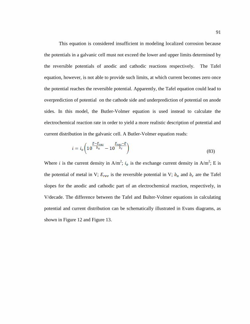
91
This equation is considered insufficient in modeling localized corrosion because
the potentials in a galvanic cell must not exceed the lower and upper limits determined by
the reversible potentials of anodic and cathodic reactions respectively. The Tafel
equation, however, is not able to provide such limits, at which current becomes zero once
the potential reaches the reversible potential. Apparently, the Tafel equation could lead to
overprediction of potential on the cathode side and underprediction of potential on anode
sides. In this model, the Butler-Volmer equation is used instead to calculate the
electrochemical reaction rate in order to yield a more realistic description of potential and
current distribution in the galvanic cell. A Butler-Volmer equation reads:
(83)
Where is the current density in A/m2; is the exchange current density in A/m2; E is
the potential of metal in V; is the reversible potential in V; and are the Tafel
slopes for the anodic and cathodic part of an electrochemical reaction, respectively, in
V/decade. The difference between the Tafel and Bulter-Volmer equations in calculating
potential and current distribution can be schematically illustrated in Evans diagrams, as
shown in Figure 12 and Figure 13.

92
Figure 12. Potential/current distribution predicted by the Tafel equation.

93 Figure 13. Potential/current distribution predicted by the Butler-Volmer equation.
As argued by Nešić et al., all cathodic reactions in a CO2 aqueous solution are
thermodynamically equivalent to H+ reduction (Reaction (79)).13 Therefore, the
reversible potential of all cathodic reactions can be calculated using the Nernst equation:
(87)
Where is the reversible potential of H+ reduction at standard conditions; is the
partial pressure of hydrogen gas on the steel surface in bar and is H+concentration at
the steel surface in mol/L.
For an anodic reaction, the reversible potential is given by the Nernst equation as:
(84)
where is the surface concentration of Fe2+ in mol/L.
The exchange current densities of electrochemical reactions are functions of the
surface concentrations of corresponding species. In the earlier studies, an arbitrary value
of current density and potential along the E-i curves of corresponding reactions have been
used to formulate the Tafel equations for anodic and cathodic reactions, as shown in
Table 1. In this work, in order to construct the Butler-Volmer equation, true reversible
potential and exchange current density must be used. The exchange current density of
each electrochemical reaction can be obtained with the knowledge of the reversible
potential, the reference current and potential along the E-i curve and the Tafel slope. The
detailed equation derivation for exchange current densities of anodic and cathodic

94 reactions are shown in Appendices 2 and 3, respectively. The parameters used for
calculating the electrochemical reaction kinetics in this model are listed in Table 2.
Compared to the Tafel equation used in the previous model, partial pressure of hydrogen
gas here affects both the reversible potential and the exchange current density of the
cathodic reactions; Fe2+ concentration, on the other hand, impacts the reversible potential
and exchange current density of the anodic reaction. This is not surprising because, with
the Bulter-Volmer equation, the cathodic and anodic reaction kinetics thereby become
functions of hydrogen gas oxidation and Fe2+ deposition respectively.
Table 1. The electrochemical parameters used for Tafel equation* in the previous model
where the current density is calculated as
Reaction
Reference current density /A/m2
Reference potential ( )/V Tafel slope (b) /V/decade Reaction
Reference current density /A/m2
Reference potential ( )/V Tafel slope (b) /V/decade Reaction
Reference current density /A/m2

95 Reference potential ( )/V Tafel slope (b) /V/decade Reaction Reference current density /A/m2 Reference potential ( )/V
Tafel slope (b) /V/decade * In this Table, concentration is steel surface concentration in the unit of mol/L; T is absolute temperature in K; R is universal gas constant 8.314J/mol.K and F is Faraday constant 96485 C/mol. Table 2. The electrochemical parameters used for Butler-Volmer equation* in the current
model where current density is calculated as
Reaction
exchange current density /A/m2
reversible potential ( )/V
Anodic Tafel slope ( ) /V/decade cathodic Tafel slope ( ) /V/decade Reaction
exchange current density /A/m2
reversible potential ( )/V
Anodic Tafel slope ( ) /V/decade cathodic Tafel slope ( ) /V/decade Reaction

96 exchange current density /A/m2
reversible potential ( )/V
Anodic Tafel slope ( ) /V/decade cathodic Tafel slope ( ) /V/decade
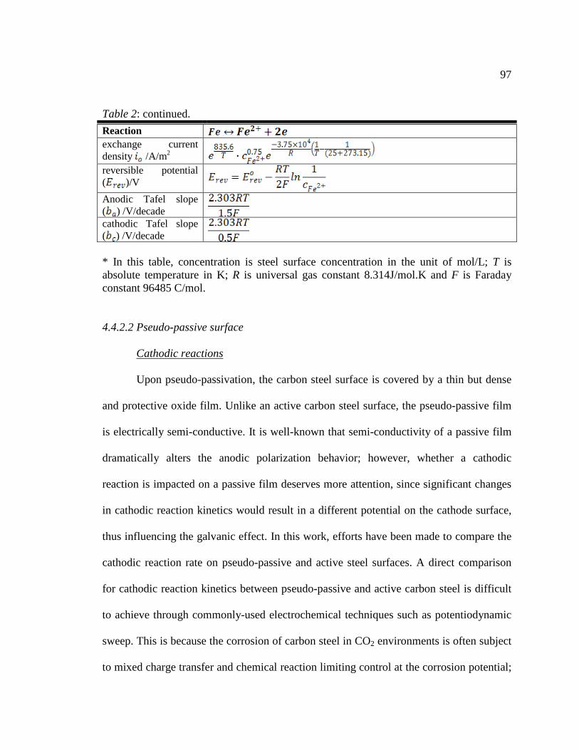
97 Table 2: continued. Reaction exchange current density /A/m2 reversible potential ( )/V
Anodic Tafel slope ( ) /V/decade cathodic Tafel slope ( ) /V/decade * In this table, concentration is steel surface concentration in the unit of mol/L; T is absolute temperature in K; R is universal gas constant 8.314J/mol.K and F is Faraday constant 96485 C/mol.
4.4.2.2 Pseudo-passive surface
Cathodic reactions
Upon pseudo-passivation, the carbon steel surface is covered by a thin but dense
and protective oxide film. Unlike an active carbon steel surface, the pseudo-passive film
is electrically semi-conductive. It is well-known that semi-conductivity of a passive film
dramatically alters the anodic polarization behavior; however, whether a cathodic
reaction is impacted on a passive film deserves more attention, since significant changes
in cathodic reaction kinetics would result in a different potential on the cathode surface,
thus influencing the galvanic effect. In this work, efforts have been made to compare the
cathodic reaction rate on pseudo-passive and active steel surfaces. A direct comparison
for cathodic reaction kinetics between pseudo-passive and active carbon steel is difficult
to achieve through commonly-used electrochemical techniques such as potentiodynamic
sweep. This is because the corrosion of carbon steel in CO2 environments is often subject
to mixed charge transfer and chemical reaction limiting control at the corrosion potential;
98 potentiodynamic sweep cannot provide direct evidence as to the charge transfer rate of a
cathodic reaction for an active steel surface. The significant difference in open circuit
potential of active and pseudo-passive carbon steel surfaces further prohibits the direct
comparison of cathodic reactions. An example of potentiodynamic sweeps performed for
stainless steel (a surrogate passive surface) and carbon steel (an active surface) is
schematically shown in Figure 14. The overlap of two cathodic sweep curves occurs in
the current limiting region, which is not surprising, as bulk concentration and
hydrodynamic conditions are the same in both cases. Clearly, no conclusion can be
deduced from this figure as to the similarity or dissimilarity of the charge transfer kinetics
for cathodic reactions on the two different surfaces. A different strategy is adopted in this
work in order to fill in the missing information. A simulation was performed using
FREECORP (presented below), a software capable of generating the Evans diagram of a
system in which potential vs. current density of electrochemical reactions can be shown.
By comparing the experimentally-obtained potentiodynamic sweep for stainless steel
with the total cathodic polarization curve generated from the software for carbon steel
under the same conditions (as shown in Figure 15), it is evident that the cathodic reaction
rate on stainless steel is not significantly different from that on the carbon steel surface.
The comparison was repeated under different conditions and similar behavior was
observed, as demonstrated in Figure 16. The experiments indicate that the thin passive
film existing on the stainless steel surface (mostly chromium oxide) does not remarkably
alter the cathodic reaction kinetics. This suggests that cathodic reaction rates are not
heavily affected by the state of metal surface. The similar behavior was also reported in

99 an independent study102 which shows the similarity of cathodic reaction rates on carbon
steel and Alloy 625 surfaces. Therefore, it can be deduced that a pseudo-passive film
formed on carbon steel would not significantly affect cathodic reaction. For practical
purposes, cathodic reaction rates on pseudo-passive surfaces can be evaluated in the same
way as for active surfaces, which are presented in Table 2.
Figure 14. Potentiodynamic sweep on stainless steel and carbon steel. Test condition: T=25°C, pH=4.1, pCO2=1 bar, stagnant solution.
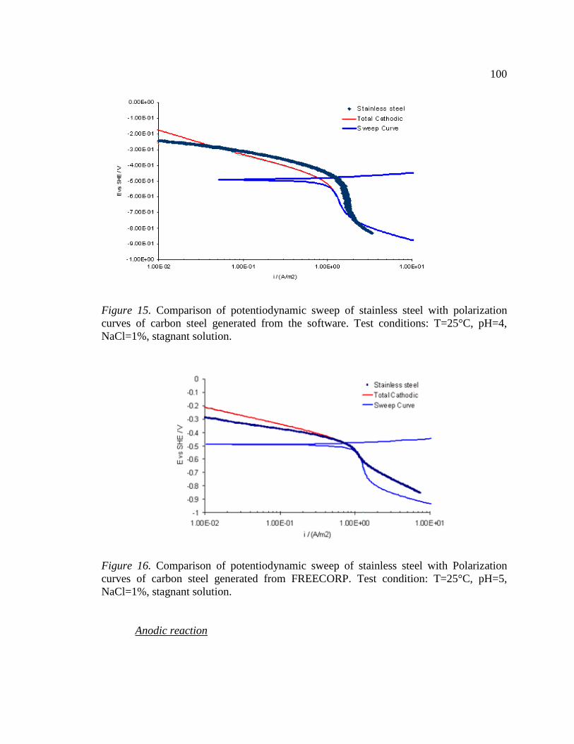
100
Figure 15. Comparison of potentiodynamic sweep of stainless steel with polarization curves of carbon steel generated from the software. Test conditions: T=25°C, pH=4, NaCl=1%, stagnant solution.
Figure 16. Comparison of potentiodynamic sweep of stainless steel with Polarization curves of carbon steel generated from FREECORP. Test condition: T=25°C, pH=5, NaCl=1%, stagnant solution.
Anodic reaction

101
Anodic reaction kinetics on a pseudo-passive surface are key in determining
localized corrosion rates, as pseudo-passive current density causes a large shift of metal
potential towards the positive direction and creates a potential difference between the
active surface of the anode and the pseudo-passive surface of the cathode. The smaller
the pseudo-passive current density is, the higher the potential difference will be, which
translates to a higher localized corrosion rate. Therefore, it is important to understand
what parameters affect pseudo-passive current density and how to calculate it.
As the first step in this study, electrochemical tests were conducted in the hope of
determining important environmental factors that affect pseudo-passive current density
and providing a guide for modeling pseudo-passive current density as a function of
relating parameters.
A cyclic polarization technique was utilized in this work to measure the pseudo-
passive current density under various conditions. The test procedure follows the ASTM
standard G61-86.103
In addition to potential, pH, temperature and chloride concentration have been
reported to play major roles in determining pseudo-passive current density. In order to
understand the effect of individual parameters and any interactions among them, a
factorial experimental design technique104 was adopted to help with test matrix design
and the statistical analysis of test results. The test procedure, results and results analysis
are presented in Appendix 4.
The results of the factorial effect analysis on pseudo-passive current density are
summarized in Table 3. According to the factorial experimental design theory, a higher

102 value of effect (irrespective of its sign) signifies more effect of the corresponding
parameter on the pseudo-passive current density. Clearly, pH and temperature have the
most significant effect on pseudo-passive current density, while the effect of Cl-
concentration is marginal. The interaction between pH and temperature seems to be
another important factor. Based on the experiments, it can be concluded that the effect of
Cl- concentration on pseudo-passive current density of carbon steel in CO2 environments
is negligible. Judging from the sign of the effects, it is evident that higher pH leads to a
smaller pseudo-passive current density, while higher temperature causes an increase in
pseudo-passive current density. This implies that a more protective pseudo-passive film is
formed under higher pH and lower temperature. It should be mentioned that, as an
electrochemical parameter, pseudo-passive current density is inherently related to
potential. Therefore, the effect of potential was intentionally excluded in the test matrix
in order to reduce the cost and numbers of experiments.
Table 3. Effect of factors on pseudo-passive current density Factors Effect
pH -23.15
T 17.99
pH & T -18.26
[Cl-] 2.64
pH & [Cl-] -2.61
T & [Cl-] 5.89
pH & T & [Cl-] -5.86
Equipped with the understanding gained from the experiments, a mechanistic
model was developed to calculate the pseudo-passive current density as related to pH,

103 temperature and potential. Apparently, a constant value of pseudo-passive current density
is not sufficient to satisfy the modeling needs of a complex CO2 corrosion system, as
surface conditions on a pseudo-passive surface, including pH and potential, change with
time. A mechanistic model is expected to provide a more appropriate response of pseudo-
passive current to change in environmental parameters.
In this work, pseudo-passive current density is determined by implementing the
Point Defect Model, originally developed by Macdonald et al. 28-31 and modified by
Camacho et al., 38 into the carbon steel/CO2 system. Detailed model development is given
in Appendix 5. The model was calibrated against an experimental database in order to
obtain the values of parameters used in the model equation. The database contains a
number of measured galvanic current densities under different conditions, which were
obtained from artificial pit tests.105 Some comparisons for the predicted and measured
galvanic current density are illustrated in section 4.7.2. The derived equation reads:
(85)
It can be seen that the model is consistent with the results of factorial
experimental analysis. Potential, pH and temperature are the three parameters included in
the model equation; and higher pH and lower temperature would lead to a smaller
pseudo-passive current density. Equation (85) also suggests that pseudo-passive current
density increases with increasing potential, which qualitatively agrees with the classic
electrochemical theory.

104 4.4.3 Mass transport
Mass transport of species in a dilute aqueous solution is governed by the law of
mass conservation, also known as Fick’s second law. In the presence of porous film, the
equation has to be modified to take into account the characteristics (e.g. porosity and
tortuosity) of the film:13
jjj RN
tc
εκε
+⋅−∇=∂∂
(86)
Where cj is the concentration of species, ε is the porosity of FeCO3 layer, κ is
permeability of FeCO3 layer which is defined as the product of porosity (ε) and tortuosity
(ξ) of the film; t is time; Nj is the flux of species and Rj is chemical reaction rate of
species.
It should be noted that Equation (86) is a universal equation describing mass
transport of species in the solution with and without a porous FeCO3 layer. In the absence
of FeCO3 layer, the porosity and tortuosity of FeCO3 in Equation (86) both simply take
the constant value of 1.
The first term on the RHS of equation (86), flux of species, is given by:
vcFcuzcDN jjjjjm
j j+∇−∇−= φ (87)
Where mj
D is the molecular diffusion coefficient; jz is the electrical charge; φ is the
electrostatic potential in the solution; F is the faraday constant; v is the in-situ flow
velocity and ju is the mobility of species. For a dilute solution, the value of mobility is
given by:

105
RTD
um
jj= (88)
Where R is universal gas constant and T is absolute temperature.
Equation (87) suggests that the flux of species is contributed by three
components: molecular diffusion, electro-migration and convection.
In a dilute solution, species can freely diffuse in the solution without coupling
with each other. Therefore, modeling molecular diffusion is straightforward, requiring
only the knowledge of a molecular diffusion coefficient.
Table 4 lists the molecular diffusion coefficients of species commonly existing in
the corrosion system of interest at 25°C. Most of the diffusion coefficients were collected
and compiled by Nešić et.al,13 with the exception of hydrogen gas. Hydrogen gas is
simulated in this model to yield the partial pressure of hydrogen gas at the steel surface,
which is required by the Butler-Volmer equation for describing the electrochemical
reaction kinetics. The diffusion coefficients are adjusted as functions of temperature and
solution viscosity using Einstein-Stokes law:
(89)
Where is the diffusion coefficient at reference temperature; and are system
temperature and reference temperature in K respectively; and are solution
viscosity under system and reference conditions in Pa.s, respectively.
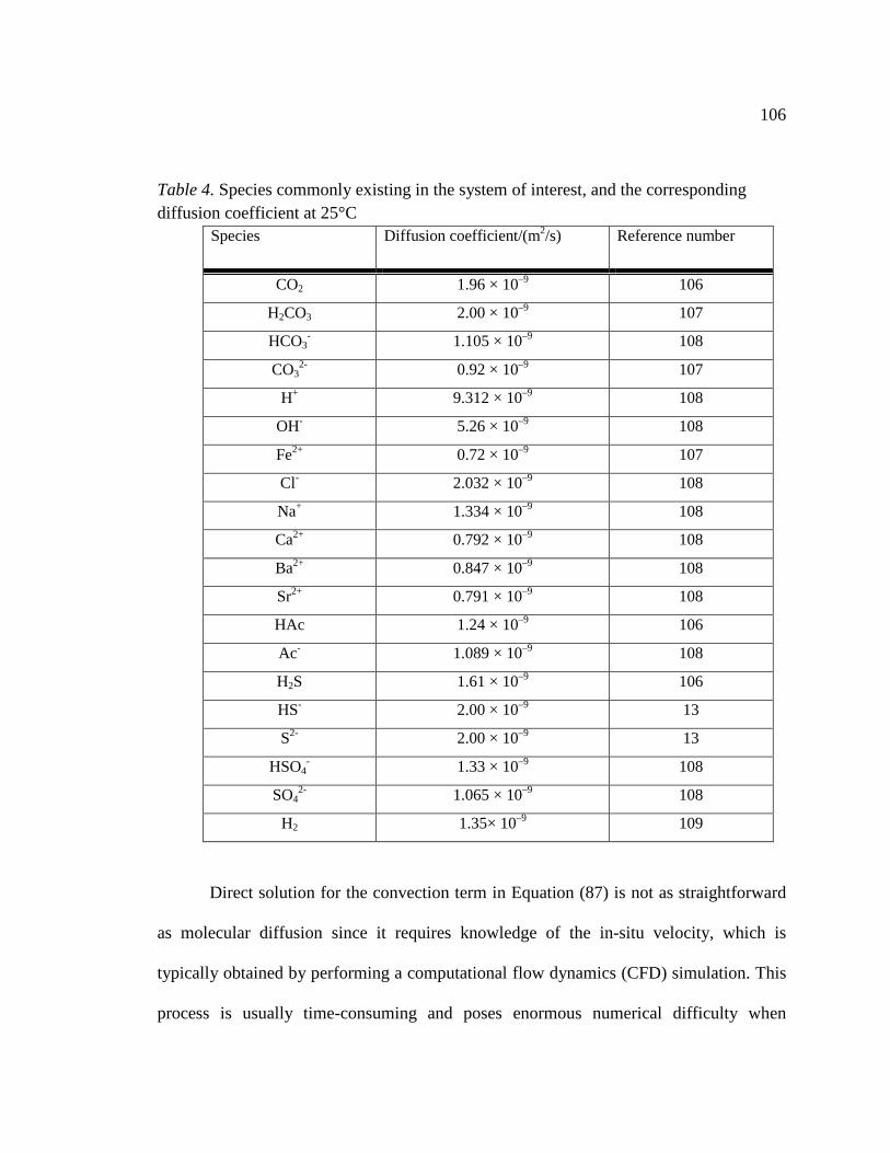
106
Table 4. Species commonly existing in the system of interest, and the corresponding diffusion coefficient at 25°C
Species Diffusion coefficient/(m2/s) Reference number
CO2 1.96 × 10⁻⁹ 106
H2CO3 2.00 × 10⁻⁹ 107
HCO3- 1.105 × 10⁻⁹ 108
CO32- 0.92 × 10⁻⁹ 107
H+ 9.312 × 10⁻⁹ 108
OH- 5.26 × 10⁻⁹ 108
Fe2+ 0.72 × 10⁻⁹ 107
Cl- 2.032 × 10⁻⁹ 108
Na+ 1.334 × 10⁻⁹ 108
Ca2+ 0.792 × 10⁻⁹ 108
Ba2+ 0.847 × 10⁻⁹ 108
Sr2+ 0.791 × 10⁻⁹ 108
HAc 1.24 × 10⁻⁹ 106
Ac- 1.089 × 10⁻⁹ 108
H2S 1.61 × 10⁻⁹ 106
HS- 2.00 × 10⁻⁹ 13
S2- 2.00 × 10⁻⁹ 13
HSO4- 1.33 × 10⁻⁹ 108
SO42- 1.065 × 10⁻⁹ 108
H2 1.35× 10⁻⁹ 109
Direct solution for the convection term in Equation (87) is not as straightforward
as molecular diffusion since it requires knowledge of the in-situ velocity, which is
typically obtained by performing a computational flow dynamics (CFD) simulation. This
process is usually time-consuming and poses enormous numerical difficulty when

107 coupled with mass transport simulation. This is mainly due to the fact that the flow
boundary layer is much thicker than the diffusion boundary layer for a water system.
Therefore, special solving strategies must be pursued for proper coupling of CFD and
mass transport simulation. To reduce the numerical effort and expedite the calculation,
Nešić et al. have suggested a simplified way to estimate the convection effect,13 which is
adopted in this model. This is achieved by replacing the convective flux with a turbulent
diffusive-like flux in the computation domain, as shown in Equation (90):
(90)
Where is the turbulent diffusion coefficient, which is a function of the distance from
the solid surface (bare steel or FeCO3 layer) and can be calculated as:
(91)
Where is the diffusion layer thickness in m; is the thickness of FeCO3 layer in m;
and x the distance away from solid surface in m.
Combining Equations (87) and (90), the fluxes of species can then be calculated
by:
φ∇−∇−= jjjjeff
j FcuzcDNj
(92)
Where effj
D is the effective diffusion coefficient account for both molecular diffusion and
turbulent diffusion effects and is given by .

108 Within the porous FeCO3 layer it is argued that there is no flow and turbulence
and species can travel through the pores driven only by molecular diffusion and electro-
migration.13
The flux due to electro-migration can usually be neglected in cases of uniform
corrosion. The potential gradient generated by different diffusion rates of species is easily
annihilated by large amounts of supporting species, such as Na+ and Cl−. However, it
would be unacceptable to neglect the electro-migration effect in localized corrosion due
to the fact that significant potential difference might exist between anode and cathode
which could drive charged species to move at appreciably different rates.
The second term on the RHS of Equation (86) accounts for chemical reaction
rates of species. As shown earlier, various species are coupled together in Reactions (52)
through (55); therefore, mass transport equations for various species have to be solved
simultaneously. The mathematical technique used to account for the chemical reaction
rates is given by Nešić et al.13 and has been previously described in section 4.4.1.
Calculation of mass transport is carried out in a pre-defined domain, the height of
which equals the thickness of diffusion boundary layer. The thickness of diffusion
boundary layer is given as:110
df8/7Re25 −=−δδ (93)
Where δ is the thickness of diffusion boundary layer, fδ is the thickness of FeCO3 layer,
Re is the Reynolds number and d is the hydraulic diameter.
Although a 2D domain would be preferable for simulating a galvanic cell, mass
transport equations are solved in two 1D domains for the anode and the cathode
109 separately, stretching from the steel surface to the diffusion boundary layer/ bulk solution
interface. Anode and cathode are then coupled together to solve the potential/current
distribution in a 2D domain. This simplification is made due to the lack of CFD
(computational fluid dynamic) simulation in the model, which would be required for the
convective flow in the streamwise direction (convective flow in normal-wall direction
can be approximated by turbulent diffusivity) if a 2D domain were to be used for mass
transport simulation. This simplification is considered acceptable because the
concentration gradients in the direction normal to the metal surface are much larger than
that those in the streamwise direction. Therefore, neglecting mass transport in the
direction parallel to the metal surface would not significantly affect the electrochemical
reaction kinetics on the metal surface.
Outside the diffusion boundary layer, all species are considered to be well-mixed
by turbulent flow; therefore, little concentration gradients are expected. For this reason,
the boundary conditions for the upper end of the computational domain are taken as the
bulk concentrations of species. The fluxes of species are used to specify the boundary
condition at the metal surface. For species not involved in electrochemical reactions, zero
flux is imposed; for corrosion-related species, e.g. H+, H2, H2CO3, HCO3-, HAc, Ac- and
Fe2+, etc., fluxes can be obtained from electrochemical reaction rates:
Fzi
Nj
jj = (94)

110 Where ji is the electrochemical reaction rate, which is dependent on the surface
concentration of corrosive species and on the metal surface potential, as illustrated in
Table 2.
As a transient simulation, initial conditions for mass transport equations are taken
to be the concentrations with which chemical equilibrium is satisfied.
Figure 17 shows the computational domain together with the governing equation
used in the model.
Figure 17. Illustration of computation domain and governing equation for mass transport simulation.
4.4.4 FeCO3 layer Growth
The equation governing FeCO3 layer growth was previously developed by Nešić
et al. 14 based on mass conservation of FeCO3 in the solution, as shown in Equation (95).
111 In this equation FeCO3 layer growth is characterized by the change in porosity. The
higher the porosity, the more porous the FeCO3 layer, and vice versa. The value of
porosity is bounded between 0 and 1. A value of 1 indicates that no FeCO3 layer is
present, while a value of 0 implies that the space is completely sealed by FeCO3 layer and
no species can travel through. This equation suggests that growth of FeCO3 layer is
attributed to two factors: FeCO3 precipitation and corrosion. Depending on the relative
values of these two terms, FeCO3 layer can be either protective or non-protective, which
is consistent with the concept of scaling tendency.65 It is important to note that when
supersaturation of FeCO3 is less than 1, the precipitation rate in Equation (95) is replaced
with the dissolution rate. Detailed information regarding this equation can be found in
the original paper14 and will not be described here.
xCRR
Mt SFeCO
SFeCO
SFeCO
∂∂
−−=∂∂ ε
ρε
)()(
)(3
3
3 (95)
Where )(3 SFeCOM and )(3 SFeCOρ are the molar mass and density of FeCO3 respectively, CR
is the corrosion rate in proper unit, ε is the porosity of FeCO3 layer, t and x are the
coordinates in time and space.
As explained by Nešić et al., the second term on the RHS of Equation (95)
accounts for the moving boundary created by the corrosion process, which poses a
convective-like effect in the equation.14 It is well-recognized that a convective term
contributes to numerical instability in solving a partial differential equation. The simplest
and most common way to avoid numerical instability is by implementing a first-order
upwind scheme in which interfacial parameters are evaluated by the corresponding values
112 in the neighboring upstream grid.111 However, this scheme has only first-order accuracy
and could easily lead to “false diffusion”.111 As argued by Lee, 112 for equations lacking a
physical diffusion term, a simple upwinding scheme would generate significant
numerical diffusion and introduce an unacceptable level of numerical error due to the
hyperbolic nature of the equation and the very small CFL
number( ). In recent years, much attention has been directed to
this issue and a number of higher-order schemes have been proposed to achieve both
accuracy and stability associated with convective terms. In the previous model, the
second-order Koren scheme with a flux limiter function was used to deal with the
convective term (CR) in Equation (95). In this work, efforts were made to investigate the
performance of this scheme against other higher-order schemes. A total of 6 schemes (2nd
order upwind,113,114 KOREN,115,116 HOAB,117 Superbee,118 OSPRE,119 MUSCL120,121) are
compared in the context of Equation (95). All of the schemes evaluate the interfacial
parameter using a specific form of second-order flux limiter functions; the
implementation of these schemes is well-explained by Waterson and Deconinck.122
Figure 18 shows one example of predictions made using various schemes. Figure 19
shows the corresponding corrosion rate history predicted using different schemes. It can
be seen that, apart from the second-order upwind, all schemes provide comparable
predictions on FeCO3 layer morphology and corrosion rate. Therefore it was decided that
the Koren scheme should be kept in the model as a means of dealing with the convective
term in Equation (95).

113
Figure 18. Comparison of surface porosity of FeCO3(95)
layer with different high-order schemes for convective term in Equation . Simulation condition: temperature 80°C, CO2 partial pressure 1 bar, liquid velocity1m/s, pipe diameter 0.1m, bulk super saturation of FeCO3
about 0.5 and bulk pH 6.5.
Figure 19. Comparison of corrosion rate with different high-order schemes for convective term in Equation (95). Simulation condition: temperature 80°C, CO2 partial pressure 1 bar, liquid velocity1m/s, pipe diameter 0.1m, bulk super saturation of FeCO3
about 0.5 and bulk pH 6.5.
0
0.1
0.2
0.3
0.4
0.5
0.6
0.7
0.8
0.9
1
0 200 400 600 800 1000 1200 1400 1600
stee
l sur
face
Por
osity
Time,min
porosity-2nd upwindporosity-HOABporosity-Korenporosity-Superbeeporosity-OSPREporosity-MUSCL
0
0.5
1
1.5
2
2.5
3
3.5
4
0 200 400 600 800 1000 1200 1400 1600
CR
,mm
/yr
Time,min
CR-2nd upwindCR-HOABCR-KorenCR-SuperbeeCR-OSPRECR-MUSCL

114 Equation (95) is solved in the same 1D domain as that used for the mass transport
equation (Equation (86)). As argued by Nešić and Lee,14 although the detailed structure
of a FeCO3 layer in a 2D or even 3D domain would be hard to simulate, it is the overall
effect of FeCO3 layer that matters; therefore, 1D simulation of FeCO3 layer growth is
considered to be sufficient for CO2 corrosion modeling.
At the FeCO3 layer / metal surface interface, the porosity is considered to be 1, as
the corrosion process, although slow, continuously creates voids underneath the FeCO3
layer. At the other boundary (between the diffusion boundary layer and the bulk
solution), it is assumed that no FeCO3 can grow onto the boundary and out of the domain;
therefore, porosity of FeCO3 maintains at 1.
Figure 20 shows the computational domain along with the governing equation for
FeCO3 layer-growth simulation.
Figure 20. Illustration of computation domain and governing equation for FeCO3
layer growth simulation.

115 4.4.5 Pseudo-passivation/repassivation
Pseudo-passivation of carbon steel is considered to be a fast process, the
occurrence of which is determined based on thermodynamic criteria. Pseudo-passivation
of carbon steel in CO2 environments has been ascribed to the existence of magnetite.12 A
two-step process leading to the generation of magnetite is proposed in this model, as
shown in Equations (96) and (97):
(96)
(97)
The thermodynamic conditions for Reactions (96) and (97) can be evaluated in
terms of Gibbs free energy. The Gibbs free energy of any species can be calculated based
on the Gibbs-Helmholtz equation:
(98)
Where T is temperature in Kelvin, G, H and S are the Gibbs free energy, enthalpy and
entropy, respectively.
As shown by Cheng et al. 123, Equation (98) can be transformed into a more
practical form by relating heat capacity of the species to enthalpy and entropy:
(99)
Where ; is heat capacity.
Empirical correlations are usually available for heat capacity of various species as
a function of temperature, which can be found in many thermodynamic handbooks. For
116 iconic species involved in Reactions (96) and (97), namely, H+ and Fe2+, the correlation
proposed by Criss and Cobble124 is used:
(100)
(101)
(102)
Where a and b are entropy constants; is the standard state entropy, is the ionic
entropy on the absolute scale and is the ionic charge.
Table 5 lists the entropy constants (a and b in Equation (101)) for different types
of ionic species, originally given by Criss and Cobble.124
Polynomial equations were obtained to calculate a and b by performing linear
regression on the data listed in Table 5.
(103)
(104)
Combining Equations (99) through (102), the Gibbs free energy of ionic species
at any temperature is given by:123
(105)
For elements and compounds involved in Reactions (96) and (97) such as H2O,
Fe3O4 and Fe(OH)2, heat capacity can be calculated as a polynomial function of
temperature:

117
(106)
By substituting Equation (106) into Equation (99), the Gibbs free energy of
elements and compounds can be calculated as:123
(107)
The parameters used in this model to calculate the Gibbs free energy of the
species involved in Reactions (96) and (97) are listed in Table 5.
Table 5. Parameters used for determination of the Gibbs free energy of species associated with pseudo-passivation
Species
Parameters
Ionic species Elements and compounds
H+ Fe2+ H2O Fe3O4 Fe(OH)2
, x10-3J/mol 0 -78.9 -237.129 -1012.57 -491.98
, J/mol.K 0 -137.7 70 146.1 88
, J/mol.K
(EQ. (101))
a N/A N/A N/A
b N/A N/A N/A
, J/mol.K (EQ.
(106))
a N/A N/A 20.4 91.6 116.1
b x103 N/A N/A 109.2 202 8.6
c x10-6 N/A N/A 2.0 N/A -2.9
, J/mol EQ. (105) EQ. (107)
With Gibbs free energy available, the reversible potential for the electrochemical
Reaction (97) or the chemical equilibrium constant for the chemical Reaction (96) at the

118 desired temperature can easily be calculated using Equations (108) and (109),
respectively:
oorev
nFEG −=∆ (108)
eqKRTGo ln−=∆
(109)
The following equations are then used to determine the equilibrium pH or
potential at which pseudo-passive film would form in the solution of interest by taking
into account the effect of species concentrations:
+
+=
2
2
Fe
Heq a
aK (110)
(111)
Where n is number of moles of electrons involved in the electrochemical reactions,
and are the reversible potential for electrochemical reactions at real and standard
conditions, respectively, and is the equilibrium constant for chemical reactions,
and are the activities of H+ and Fe2+, respectively, which are estimated by the
corresponding concentrations.
4.4.6 Pit initiation
Since the mechanism governing pit initiation for carbon steel in CO2
environments is not clearly understood at present, in this model, a pit is initiated by
artificially removing the protective layer at a randomly determined point in time. The
stochastic nature of pit initiation is simulated using a Weibull distribution random
function. Ascher125 defines the initiation time for each of the pits on a coupon as the time
119 at which the first failure of the system occurs. Following his reasoning, the Weibull
distribution function seems to be a good option for simulating random behavior of pit
initiation as it is the most widely used function in the field of failure analysis. For
example, DNV standard RP G101 describes a means of determining the probability of
failure based on the Weibull distribution.126 One of the unique advantages of Weibull
distribution function is that, depending on the parameters provided, this function can
exhibit the characteristics of other commonly used distribution functions such as normal,
lognormal, etc. This provides flexibility in controlling how pit initiation behaves with
respect to time.
It should be pointed out that, since this model performs calculations for only two
points (anode and cathode) on a metal surface, it is not intended to simulate the random
behavior related to the location of pit initiation.
A two-parameter Weibull distribution function is defined as:
β
αβ
ααβ
−−
=
x
exxWe1
)( (112)
Where We is the Weibull function, x is the independent variable, α is the scale
parameter, β is the shape parameter.
The scale and shape parameters are related to mean and standard deviation of the
distribution in the following ways:
+Γ=β
αµ 11 (113)
120
+Γ−
+Γ=
ββασ 1121 222
(114)
Where µ is the mean value, σ is the standard deviation, Γ is the gamma function,
which is defined as:
(115)
Scale parameter and shape parameter can be obtained by solving Equations (113)
and (114) based on the values of mean and standard deviation. Once scale and shape
parameters are obtained, a Weibull distribution random number can be generated based
on a uniform distribution random number,127 which is normally given as a built-in
function in most software packages, as shown in Equation (116):
( )[ ]βα1
1ln xy −−⋅= (116)
Where y is the Weibull distribution random number and x is the uniform distribution
random number between 0 and 1.
Currently, a mean value of 2 hours after pseudo-passivation and a standard
deviation of 0.5 hours are used to generate the time for pit initiation. These values are
arbitrarily set and can easily be changed according to experimental findings.
4.4.7 Pit propagation
Pit propagation is driven by the potential difference between anode and cathode.
The pit propagation rate is governed by the metal potential at the steel surface. Due to the
galvanic effect, the metal potential can accelerate the corrosion rate on the anode and
decelerate that on the cathode. Due to the separation of anode and cathode, the solution

121 resistance between anode and cathode also plays an important role in the pit propagation
stage.
The potentials on the metal surface and in the liquid layer above the metal can be
obtained by solving the Laplace equation governing potential distribution in a conductive
medium:
( ) 0=∇⋅∇ φκ eff (117)
Where effκ is the effective conductivity of the electrolyte account for the presence of non-
conductive FeCO3 layer, which is given by Bruggeman’s equation as:91
(118)
Where is the porosity of FeCO3 layer and is the conductivity of electrolyte without
FeCO3 layer, which can be calculated as:108
(119)
Where is Faraday constant, is the ionic charge, is the mobility and is the
concentration.
Considering:
(120)
Equation (117) suggests:
0=⋅∇ i (121)
Equation (121) indicates that there is no net current change in the solution and
that the solution always maintains electro-neutrality.
122
It should be noted that the accurate form of the governing equation for
electrostatic potential distribution is given by Poisson’s equation:108
∑−=∇j
jjczFξ
φ2 (122)
where ξ is the permittivity of the electrolyte. This equation implies that potential
distribution is related to the charge separation of species in the solution. However, it has
been argued that in an electrochemical system, potential distribution occurs on a much
shorter time scale than mass transfer. Heppner80 estimated that the time required to
electrically neutralize an electrolyte is 10-8 seconds. For water system, the quotient of F/ξ
is very large, which physically indicates that any small separation of charge would
generate a significant potential gradient which tends to rapidly restore the system to the
state of electro-neutrality. The strong force resulting from a large electrostatic potential
gradient can eliminate any charge imbalance at a speed much faster than that of mass
transport. Therefore, it is common practice to assume that electroneutrality is preserved at
any point of time. Mathematically, this means that Equation (122) can be safely replaced
with Equation (117) without introducing major errors.
Unlike in a mass transport process where a 1D domain is acceptable, a significant
potential gradient can be present both in directions perpendicular and parallel to the metal
surface. Therefore, it is essential to calculate the potential distribution in a 2D domain as
shown in Figure 21; the height of which is equal to the thickness of the liquid layer.

123
Figure 21. Computation domain and governing equation with boundary conditions for electrostatic potential distribution in aqueous solution.
The boundary condition on the steel surface is given by Kirchhoff’s law:
∑ ∇−= φκji (123)
Where ji is the current density of individual electrochemical reactions on the metal
surface, which can be calculated by the equations presented in Table 2.
For other boundaries (the left, right and upper walls of the computation domain),
normal current density is set to zero. The right wall is far away from the metal surface
and charged species would therefore not be able to reach the boundary; the upper wall
defines the location where liquid phase (and therefore charged species) ends; the left
boundary maintains zero current density due to symmetrical configuration.
It is worth mentioning that although Equation (117) applies to both uniform and
localized corrosion, it is not solved for uniform corrosion in the model. This is because
the potential is uniformly distributed on the steel surface due to the close proximity of

124 anode and cathode in a uniform corrosion cell. This uniform potential can be readily
obtained based on the charge balance of anodic and cathodic reactions, as shown in
Equation (124):
∑∑ =cathodicanodic
ii (124)
where i is current density of anodic or cathodic reactions.
With the knowledge of metal potential, the anodic dissolution rate can be
calculated using the iron oxidation reaction shown in Table 2.
For localized corrosion cases, potential is calculated on multiple points along the
anode and cathode surfaces. In order to couple the 2D simulation of potential distribution
with the 1D simulation of mass transport, the average current density on the anode or
cathode surface is calculated to provide the boundary conditions for mass transport
Equation (86). This is done by replacing Equation (94) with:
FzA
AiN
j
iiij
j ⋅
⋅=∑
(125)
where is the current density related to the jth species at the ith location, is the steel
surface area at the ith location and is the total area of anode or cathode.
4.5 Numerical technique
The governing equations for mass transport and FeCO3 layer growth are solved in
two 1D domains as sketched in Figure 17 and Figure 20. It should be noted that one mass
transport equation is needed for each species in solution. To simulate a real system,
multiple mass transport equations are coupled and solved simultaneously. Simulating a

125 CO2 aqueous system typically requires solving 10 equations or more. The governing
equations are discretized using the control volume method in the predefined 1D domain
with a non-uniform grid as sketched in Figure 22. Denser control volumes are placed near
the steel surface where the highest fluxes are expected; as the grid approaches the bulk,
less control volumes are used. With the control volume method described by Patankar,111
the governing partial differential equations are converted into a series of algebraic
equations in each control volume. Equations (86) and (95) can be respectively discretized
as:
(126)
(127)
where subscripts P, P-1/2 and P+1/2 represent the control volume P and its adjacent
upstream and downstream interfaces respectively as illustrated in Figure 22. Superscript
“o” signifies the known variables from the previous time step and the variables without
“o” refer to the present time, which are unknowns and are to be solved for.
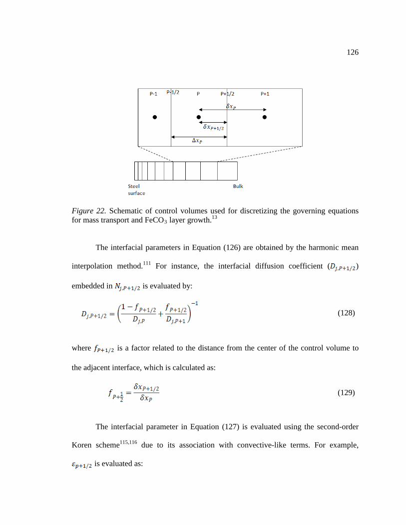
126
Figure 22. Schematic of control volumes used for discretizing the governing equations for mass transport and FeCO3 layer growth.13
The interfacial parameters in Equation (126) are obtained by the harmonic mean
interpolation method.111 For instance, the interfacial diffusion coefficient ( )
embedded in is evaluated by:
(128)
where is a factor related to the distance from the center of the control volume to
the adjacent interface, which is calculated as:
(129)
The interfacial parameter in Equation (127) is evaluated using the second-order
Koren scheme115,116 due to its association with convective-like terms. For example,
is evaluated as:
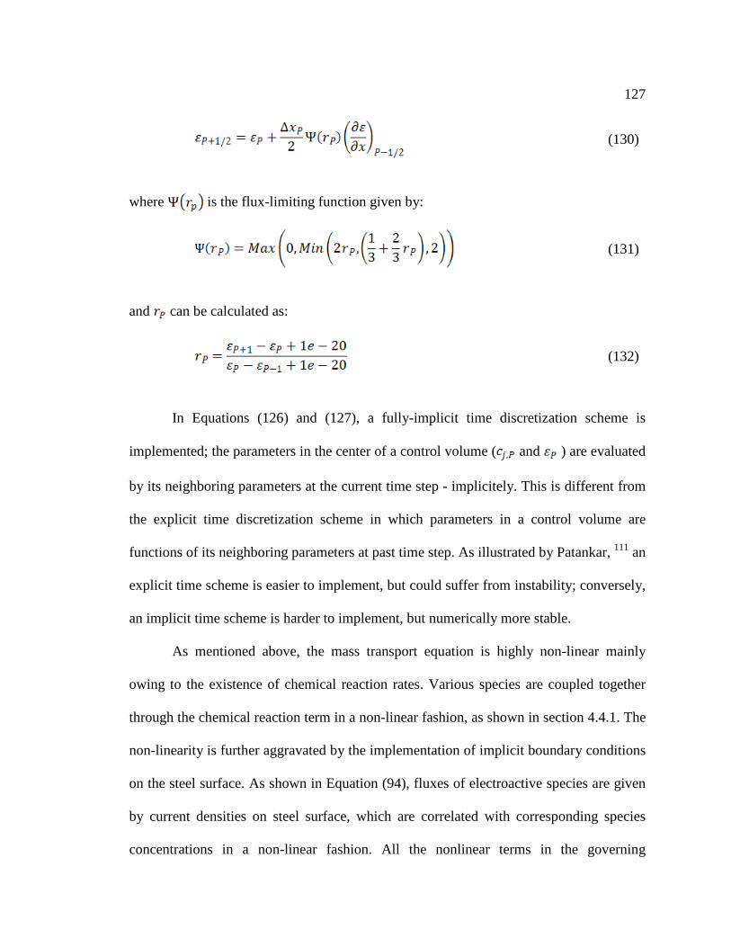
127
(130)
where is the flux-limiting function given by:
(131)
and can be calculated as:
(132)
In Equations (126) and (127), a fully-implicit time discretization scheme is
implemented; the parameters in the center of a control volume ( and ) are evaluated
by its neighboring parameters at the current time step - implicitely. This is different from
the explicit time discretization scheme in which parameters in a control volume are
functions of its neighboring parameters at past time step. As illustrated by Patankar, 111 an
explicit time scheme is easier to implement, but could suffer from instability; conversely,
an implicit time scheme is harder to implement, but numerically more stable.
As mentioned above, the mass transport equation is highly non-linear mainly
owing to the existence of chemical reaction rates. Various species are coupled together
through the chemical reaction term in a non-linear fashion, as shown in section 4.4.1. The
non-linearity is further aggravated by the implementation of implicit boundary conditions
on the steel surface. As shown in Equation (94), fluxes of electroactive species are given
by current densities on steel surface, which are correlated with corresponding species
concentrations in a non-linear fashion. All the nonlinear terms in the governing

128 equation(s) are linearized using Taylor series expansion, keeping only the constant and
the linear term. As an example, the chemical reaction term can be linearized as:
(133)
Where is the derivative of chemical reaction rate with respect to
involved species concentrations, which is evaluated at the concentrations obtained at the
previous time step.
The discretized first-order algebraic equations are assembled into a matrix in the
form of AX=B and solved simultaneously to obtain the concentrations and porosity of
FeCO3 in all control volumes. In this model, an LU method is implemented to solve the
matrix.
The governing equation for potential distribution (Equation (117)) is solved in a
2D domain as shown in Figure 21. A line-by-line method is implemented to solve the
equation.111 In this method, the governing equation is discretized in the same way as
presented above:
(134)
where upper case subscripts (E, W, N, S, and P) refer to the center of control volume and
lower case subscripts (e, w, n and s) represent the interfaces. and are the size of the
control volumes in the E-W and N-S directions, respectively. The notations are
schematically illustrated in Figure 23.
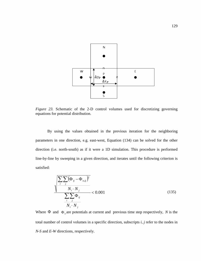
129
Figure 23. Schematic of the 2-D control volumes used for discretizing governing equations for potential distribution.
By using the values obtained in the previous iteration for the neighboring
parameters in one direction, e.g. east-west, Equation (134) can be solved for the other
direction (i.e. north-south) as if it were a 1D simulation. This procedure is performed
line-by-line by sweeping in a given direction, and iterates until the following criterion is
satisfied:
( )
001.0
2,
<
⋅
Φ
⋅
Φ−Φ
∑∑
∑∑
ji
i jij
ji
i jijoij
NN
NN (135)
Where Φ and oΦ are potentials at current and previous time step respectively, N is the
total number of control volumes in a specific direction, subscripts i, j refer to the nodes in
N-S and E-W directions, respectively.

130 4.6 Solving strategy
Figure 24 shows the calculation flow chart used in this model. The program starts
with the calculation of metal potential under initial conditions (temperature, pressure,
water chemistry, water velocity, etc.). This is followed by solving mass transport
equations for various species and FeCO3 layer growth equations in the predefined 1D
domains for anode and cathode sequentially. In solving mass transport equations, the
metal potential is used to generate fluxes of species, which are used to define the
boundary conditions for the governing equations. The Laplace equation for potential is
then solved in a predefined 2D domain in order to obtain the potential distribution. The
updated potentials allow for the calculation of anodic and cathodic reaction rates, which
can be used to generate the corrosion rate. The calculation then advances in time and
starts another cycle of calculations. Throughout the calculation, steel surface pH and
potential are constantly monitored. When surface conditions are such that pseudo-
passivation is favored, the electrochemical reaction kinetics for pseudo-passive surface
will be used to calculate the current densities. Once pseudo-passivity is achieved, the
Weibull distribution random function is activated, which will at some point in time
activate removal of the protective layer on the anode and initiate the pit. Upon pit
initiation, electrochemical reaction kinetics on the anode are switched to those for active
surface, while pseudo-passivity is maintained on the cathode.

131

132
Figure 24. Flow chart used in the localized corrosion model.
Start
Model initialization: read in parameters and generate mesh
Calculate initial metal potential
Solve for anode
jjj RN
tc
εκε
+⋅−∇=∂∂
xCRR
Mt SFeCO
SFeCO
SFeCO
∂∂
−−=∂∂ ε
ρε
)()(
)(3
3
3
Calculate corrosion rate and output results
End
No Yes
Solve for cathode
jjj RN
tc
εκε
+⋅−∇=∂∂
xCRR
Mt SFeCO
SFeCO
SFeCO
∂∂
−−=∂∂ ε
ρε
)()(
)(3
3
3
Passivation? Pit initiation?
Yes
Solve for potential ( ) 0=∇⋅∇ φκ eff
Solve for potential
∑∑ = ca ii
No
Steady state? Proceed to new time

133 4.7 Model verification and parametric study
Although the present model targets CO2 localized corrosion, it has the capability
of predicting uniform corrosion as well, as all the phenomena involved in the uniform
corrosion process (i.e. mass transfer, chemical reactions, electrochemical reactions and
FeCO3 layer growth) are present in localized corrosion. Based on the previously-built
uniform corrosion model (MULTICORP V4), a completely new version of the corrosion
prediction software package was developed (MULTICORP V5) based on the present
work with entirely new source codes designed to simulate uniform corrosion as well as
CO2 localized corrosion. A number of improvements, both in the physico-chemical and
numerical models were made for uniform corrosion simulation. New physics governing
CO2 localized corrosion was incorporated. The major improvement is in the description
of electrochemical reaction kinetics, which is now done through the use of the Butler-
Volmer equation with true exchange current density and reversible potential. This change
results in a more reasonable potential distribution in a galvanic cell, which is critical in
calculating galvanic current density. In terms of numerical changes, the main
improvement was in the use of an implicit time marching scheme in solving the
governing equation for FeCO3 layer growth (Equation (95)). This improvement enhances
the stability of the model, which would accommodate a bigger time step in the
calculation leading to less simulation time. Due to the rebuilding of the entire source
code, the new model needed to be recalibrated against with a large number of
experimental data points for uniform corrosion and with what limited data exist for
localized corrosion (all contained in the experimental database at ICMT). Overall the
134 verification showed good agreement. A few comparisons are illustrated in the section
below to facilitate further discussion of the model’s performance.
4.7.1 Uniform corrosion verification
4.7.1.1 Film free condition
Figure 25 shows the comparisons between the model and experiments for two
important factors, pH and velocity. Good agreement is evident under all conditions. This
is not surprising considering the fact that CO2 uniform corrosion is relatively well-
understood and mechanistically implemented in this model. It can be seen that corrosion
rate increases with increasing velocity and reaches a maximum value at a certain velocity,
which becomes flow-independent at still higher flow rates. This is an indication that the
corrosion process switches from mass transfer limiting to charge transfer limiting. The
model also suggests that corrosion becomes progressively less flow-independent as pH
increases. This is because, at a higher pH, corrosion is predominantly contributed by
H2CO3 reduction, a reaction controlled by CO2 hydration rate rather than by mass
transfer.

135
Figure 25. Comparisons between model and experiments for 1 bar CO2
, 20°C and various pHs and velocities.
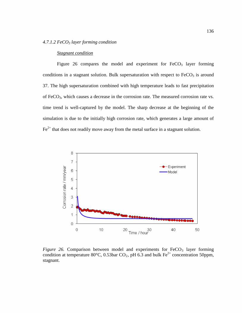
136 4.7.1.2 FeCO3 layer forming condition
Stagnant condition
Figure 26 compares the model and experiment for FeCO3 layer forming
conditions in a stagnant solution. Bulk supersaturation with respect to FeCO3 is around
37. The high supersaturation combined with high temperature leads to fast precipitation
of FeCO3, which causes a decrease in the corrosion rate. The measured corrosion rate vs.
time trend is well-captured by the model. The sharp decrease at the beginning of the
simulation is due to the initially high corrosion rate, which generates a large amount of
Fe2+ that does not readily move away from the metal surface in a stagnant solution.
Figure 26. Comparison between model and experiments for FeCO3 layer forming condition at temperature 80°C, 0.53bar CO2, pH 6.3 and bulk Fe2+
concentration 50ppm, stagnant.

137
Flowing conditions
Figure 27 compares the model prediction with a set of experiments conducted in a
glass cell with flowing conditions. Clearly, predictions fall among the variations of
experimental data, revealing the capability of the model in simulating FeCO3 growth
kinetics and their effect on the corrosion process.
Figure 27. Comparisons between the model and the experiments for flowing FeCO3 layer-forming condition at temperature 80°C, pH 6.6, 0.53bar CO2, 10ppm bulk Fe2+
and 1000rpm rotation speed.
4.7.2 Localized corrosion verification
Limited experimental data is available in the open literature for localized
corrosion rates of carbon steel corroding in CO2 solutions. More importantly, it is not
uncommon for information to be missing in open literature, and for simulation purposes

138 some assumptions have to be made. To raise the confidence level, the measurements
conducted at ICMT are adopted as the data source for model calibration. The data were
obtained in a series of artificial pit experiments conducted by Han et al.105 In these
experiments, a large ring-shaped electrode is pre-corroded in a solution with high pH and
temperature to allow the formation of dense FeCO3 layer and spontaneous pseudo-
passivation on the electrode surface. Once a stable FeCO3 layer is obtained, the electrode
is transferred into the solution of interest, and a small electrode with a freshly polished
active surface is then inserted into the hole at the center of the large electrode, forming a
galvanic cell with electric connection between two electrodes. The galvanic current is
then measured as a function of time. The test equipment is schematically shown in Figure
28. The detailed test conditions and procedures can be found in the original paper.105 It
should be stressed that these experiments recorded only the galvanic current. This should
not be confused with the anodic current density which is directly related to the localized
corrosion rate. The galvanic currents in the experiments are defined as the difference
between total anodic and cathodic current at the metal potential. From Figure 29 it is
apparent that the galvanic current (represented by Igalvanic) is smaller than the anodic
current (symbolized as Icorrcouple). Since the potential is non-uniformly distributed along
the metal surface, the model takes the average galvanic current density over the anode
surface to be used for comparison. Figure 30 shows an example of comparison between
anodic current density and galvanic current density. Anodic current density is evidently
higher than galvanic current density throughout the simulation.

139
Figure 28. Schematic illustration of the artificial pit unit used in Han et al. experiments (a) fully assembled artificial pit, (b) cutaway side view, (c) enlarged bottom view of cathode; center hole for anode, (d) detailed cross section view.105

140
Figure 29. Evans diagram depicting relationship of galvanic current and anodic current. Galvanic current is represented by Igalvanic and anodic current is symbolized by Icorr
couple
.
Figure 30. Comparison of anodic current density and galvanic current density. Simulation conditions: Supersaturation of FeCO3 0.3−0.9, T 80 ºC, CO2
0.53bar, pH 5.9-6.1, 1wt % NaCl, stagnant.
141 4.7.2.1 Stagnant condition
Figure 31 shows the measured and predicted galvanic current density in a stagnant
solution. Both model and experiments suggest pit propagation under these conditions
where supersaturation is around 1 (the condition known as the “grey zone” 1). The
galvanic current density starts off at a high value and quickly drops within short period of
time. It then slowly creeps up and reaches around 1A/m2 at the end of the simulation. The
sharp drop in galvanic current density at the beginning is due to the establishment of
mass transfer limitation which is induced by the high galvanic current density at the
moment of galvanic coupling. In a stagnant solution, the corrosion product (Fe2+)
generated from the corrosion process tends to stay at the metal surface, leading to a large
increase in supersaturation and resulting in fast precipitation on the metal surface. In such
a process, CO32- is continuously consumed by the precipitation process. In the mean time,
supplemental CO32- from the bulk solution is compromised by the large mass transfer
resistance due to the absence of convective flow. Therefore, substantial reduction of
CO32- concentration is experienced near the steel surface, which drives Reaction (30) to
give up more H+ in the solution adjacent to the anode surface. The increased solution
acidity raises the potential of the anode and leads to increased anode current density as
the corrosion process evolves. It can be expected that, as the precipitation process
continuously draws CO32- out of the solution, a shortage of CO3
2- will eventually be
experienced particularly in the vicinity of the metal surface, which will decrease the
supersaturation of FeCO3. Excessive Fe2+ on the steel surface will then start raising the
surface pH to maintain charge balance in the solution. The competing effect of

142 precipitation and charge balance will eventually reach the balance where pit propagation
can continue at a relatively stable rate. Figure 32 shows the history of a predicted surface
pH and potential at an anode to support the above arguments.
Figure 31. Comparison of galvanic current density between model and experiments for the conditions: Supersaturation of FeCO3 0.3−0.9, Temperature 80 ºC, CO2
0.53bar, pH 5.9-6.1, 1wt % NaCl, stagnant.

143
Figure 32. Surface pH and potential as a function of time. Simulation conditions: Supersaturation of FeCO3 0.3−0.9, T 80 ºC, CO2
0.53bar, pH 5.9-6.1, 1wt % NaCl, stagnant.
Figure 33 illustrates a case of pit death at FeCO3 supersaturation above 1.
Mimicking the trend exhibited in the measurement, the model predicts a progressively-
decreasing galvanic current density which eventually diminishes after about 40 hours.
The decreasing galvanic current density is due to the formation of FeCO3 layer on the
anode surface as a result of FeCO3 supersaturation above 1. The FeCO3 layer formation is
greatly enhanced by the slow mass transfer of Fe2+ in the stagnant solution. Still, it is
striking that a medium level of supersaturation in this case would cause such a rapid
decrease of galvanic current. This case further justifies the “grey zone” theory, which
suggests that a pit propagates when supersaturation of FeCO3 is around unity.

144
Figure 33. Comparison between the model and the experiment for the conditions: Supersaturation of FeCO3 3−9, T 80 ºC, pCO2
0.53bar, pH 5.6, [NaCl] =1wt%, stagnant.
4.7.2.2 Flowing condition
Figure 34 illustrates the measured and simulated galvanic current densities in a
flowing solution. It is notable that pit propagation prevails in this case with the
supersaturation value within the “grey zone”. The galvanic current density initializes at a
high value and quickly drops to about 4A/m2 due to mass transfer limitation. The
galvanic current density is then stabilized at that level in the rest of the simulation. It
worth mentioning that under flowing conditions, the galvanic current density does not
increase with time as galvanic corrosion proceeds. This is because the flow greatly
enhances the mass transfer and carries away the corrosion product (Fe2+) on the metal

145 surface, which prevents the large consumption of CO3
2- and resulting acidity in the near-
metal solution. Conversely, the model predicts a slightly higher surface pH compared to
the bulk value (pH 5.9) due to existence of excessive Fe2+ on the metal surface, as shown
in Figure 35. The surface pH variation is consistent with the trend of galvanic current,
which reflects the amounts of Fe2+ produced in the corrosion process.
Figure 34. Comparison between model and experiments for the conditions: Supersaturation of FeCO3 0.8−4, T 80 ºC, CO2
0.53bar, pH 5.9, 1wt % NaCl, 500rpm.
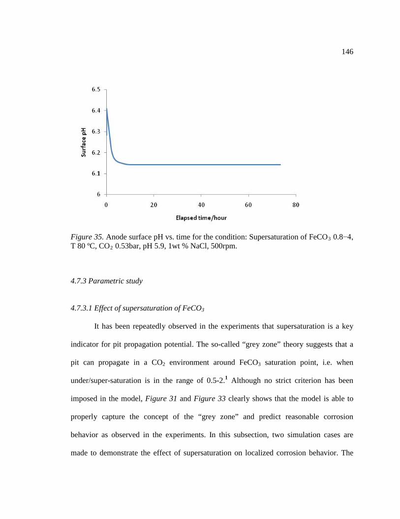
146
Figure 35. Anode surface pH vs. time for the condition: Supersaturation of FeCO3 0.8−4, T 80 ºC, CO2
0.53bar, pH 5.9, 1wt % NaCl, 500rpm.
4.7.3 Parametric study
4.7.3.1 Effect of supersaturation of FeCO3
It has been repeatedly observed in the experiments that supersaturation is a key
indicator for pit propagation potential. The so-called “grey zone” theory suggests that a
pit can propagate in a CO2 environment around FeCO3 saturation point, i.e. when
under/super-saturation is in the range of 0.5-2.1 Although no strict criterion has been
imposed in the model, Figure 31 and Figure 33 clearly shows that the model is able to
properly capture the concept of the “grey zone” and predict reasonable corrosion
behavior as observed in the experiments. In this subsection, two simulation cases are
made to demonstrate the effect of supersaturation on localized corrosion behavior. The

147 simulation conditions are: temperature 80°C, CO2 partial pressure 0.52 bar, liquid
velocity 0.5 m/s, 0.1 wt% NaCl, bulk pH 6, bulk supersaturation of FeCO3 1 and 10
respectively.
Figure 36 compares the corrosion rates for different supersaturation levels. It can
be seen that a higher supersaturation evidently shorten the time required for pseudo-
passivation, as indicated by the sharp drop in the corrosion rate at about 70 hours for
supersaturation of 10. The pseudo-passivation is attributed to FeCO3 precipitates on the
metal surface, which increases the mass transfer resistance to various species moving
towards or away from the metal surface. Particularly, this leads to a lower concentration
of H+ or higher pH on the metal surface. The onset of pseudo-passivation is triggered
upon achievement of a critical surface pH where formation of magnetite is favored, as
discussed in section 4.4.5. The sudden jump of corrosion rate shortly after pseudo-
passivation is due to pit initiation, which is achieved by artificially removing the
protective films on the anode surface, including FeCO3 layer and pseudo-passive film. In
this process, the bare active anode surface is exposed to the corrosive solution, leading to
a lower potential while the cathode remains pseudo-passivated. A galvanic cell is
therefore established between the active anode and the pseudo-passviated cathode, which
drives the anode to corrode at a substantially higher rate. It can be seen that the two
simulation cases exhibit quite different corrosion behaviors after the pit is initiated. With
lower supersaturation, pit is able to propagate in the remainder of simulation time, while
pit death is experienced with higher supersaturation irrespective of repeated pit initiation
triggered by artificial film removal. The stable pit propagation at supersaturation 1 is due

148 to the balance between FeCO3 precipitation rate and corrosion rate, which leaves the
anode surface relatively free of film coverage. At an elevated supersatuation, however,
FeCO3 precipitation proceeds faster than corrosion, which builds a more protective
FeCO3 layer on the anode surface leading to a decreasing potential difference between
anode and cathode, at some point in time, the potential difference is vanished due to
repassivation on the anode surface. The potential differences for two cases are
demonstrated in Figure 37.
Figure 36. Effect of supersaturation on localized corrosion rate. Simulation conditions: temperature 80°C, CO2
partial pressure 0.52bar, 0.1 wt% NaCl, velocity 0.2m/s, bulk pH 6.

149
Figure 37. Potential difference between anode and cathode for two simulation cases with supersaturation 1 and 10 respectively. Simulation conditions: temperature 80°C, CO2
partial pressure 0.52bar, 0.1 wt% NaCl, velocity 0.5m/s, bulk pH 6.
4.7.3.2 Effect of velocity
Velocity is an important factor in a uniform corrosion process by enhancing mass
transfer rate of corrosive species. This subsection is intended to demonstrate how velocity
can affect localized corrosion process. It should be noted that flow effect on pit initiation
is not yet built in the model. Therefore, it is not the intention of this case to discuss the
scenario related to flow induced localized corrosion. Rather, the emphasis is placed on
flow effect on pit propagation. Figure 38 shows the corrosion rate change for bulk
velocity of 0.5m/s and 1m/s. The simulation conditions are: temperature 80°C, CO2
partial pressure 0.53bar, 0.1 wt% NaCl, bulk pH 6, bulk supersaturation of FeCO3 10.
It can be seen that higher velocity largely delays pseudo-passviation. This is due
to the enhanced mass transfer rate in a fast-flowing fluid which swiftly carries away Fe2+

150 on the metal surface and effectively reduces the supersaturation of FeCO3. As a result, a
slower precipitation process is experienced with higher velocity. It can be seen that under
higher velocity, the reduced precipitation rate slows down FeCO3 layer buildup on the
anode surface irrespective of high supersaturation of FeCO3 in the bulk solution. This
leads to pit propagation throughout the simulation. On the other hand, in the lower
velocity case ,pit death is predicted shortly after pit initiation. The pit death at low
velocity is due to the accumulation of Fe2+ on metal surface leading to increased surface
supersaturation and consequent precipitation of FeCO3, which overpowers undermining
effect. This case clearly demonstrates that, once initiated, a pit tends to propagate in a
fast-moving solution but its growth is arrested in a slow-moving solution.

151
Figure 38. Corrosion rate comparison for bulk liquid velocity at 0.5m/s and 1m/s. Simulation conditions: temperature 80°C, CO2 partial pressure 0.52bar, 0.1 wt% NaCl, bulk pH 6, bulk supersaturation of FeCO3
10.
4.7.3.3 Effect of solution conductivity
Solution conductivity plays a significant role in galvanic corrosion, as it affects
potential and current distribution in a galvanic cell. Lower solution conductivity leads to
a more non-uniformly distributed potential and smaller current, while higher conductivity
results in a more spreading pattern of potential distribution and higher current. Without
the consideration of solution conductivity, the localized corrosion rate would be largely
overestimated, with the exception of the cases where solution conductivity is very high.
In this model, potential distribution is solved with solution conductivity, mass transfer
and charge transfer effect coupled together; in other words, tertiary potential distribution
can be obtained with the model. Figure 39 compares the galvanic current density of the
anode in solutions with different conductivity. Pronounced differences can be seen for
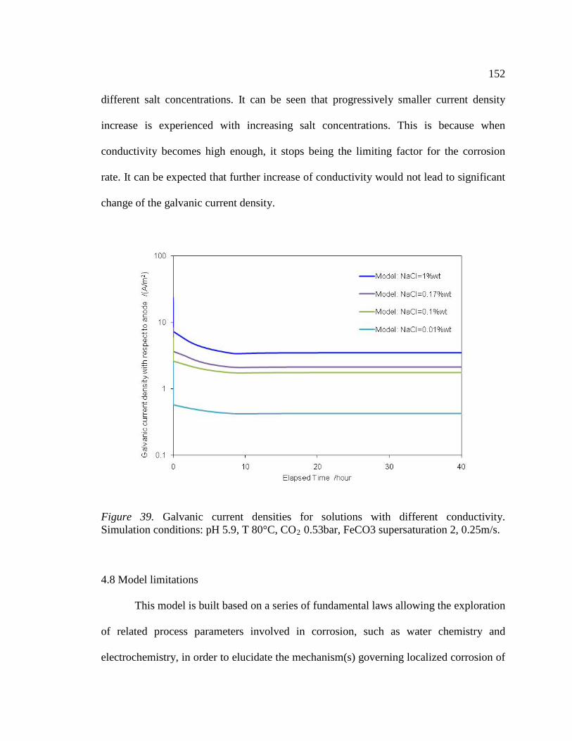
152 different salt concentrations. It can be seen that progressively smaller current density
increase is experienced with increasing salt concentrations. This is because when
conductivity becomes high enough, it stops being the limiting factor for the corrosion
rate. It can be expected that further increase of conductivity would not lead to significant
change of the galvanic current density.
Figure 39. Galvanic current densities for solutions with different conductivity. Simulation conditions: pH 5.9, T 80°C, CO2
0.53bar, FeCO3 supersaturation 2, 0.25m/s.
4.8 Model limitations
This model is built based on a series of fundamental laws allowing the exploration
of related process parameters involved in corrosion, such as water chemistry and
electrochemistry, in order to elucidate the mechanism(s) governing localized corrosion of

153 carbon steel in a CO2 environment. Calculated results have shown good agreement with
experimental results. However, like any model, the present model has certain
assumptions and limitations that must be appreciated by users in order to achieve
confident predictions.
Limitations of the current model are listed below:
This model is a “2-point model” for mass transport (1D simulation performed for two
individual points: anode and cathode) coupled with a 2D model for potential/current
distribution. Concentration gradients in the direction parallel to the metal surface are
assumed to be unimportant and are neglected.
An ideal solution is assumed, e.g., concentrations instead of activities are used for
calculation, and species independently diffuse in the solution.
Pit initiation is arbitrarily triggered, as the exact theory is still under development;
therefore, kinetics of pit initiation are not properly included.
As a pit propagates, the anode surface progressively recedes. The moving boundary
increases the distance over which diffusion occurs, which enhances the mass transfer
resistance. The effect of a moving boundary is neglected in the current model.
5. Conclusions
A transient mechanistic model has been built “from the ground up” to simulate
the CO2 localized corrosion process of carbon steel. The new model (MULTICORP V51
1 Since the availability of the source code and the application software based on the present model (MULTICORP V5) is limited to the sponsoring companies, an effort was made to provide the broader corrosion community with a free mechanistic model for internal corrosion prediction of carbon steel pipelines, built around the same theoretical concepts. This was achieved by building FREECORP software with an open source code, which is described in Appendix 6.
)
is built upon the previously developed uniform corrosion model (MULTICORP V4), in

154 which mass transfer, water chemistry, surface electrochemistry, FeCO3 layer formation
are taken into account. New physics governing localized corrosion, such as pseudo-
passivation/repassivation, galvanic coupling with solution resistance effect have been
added into the model to enable the prediction of both uniform and localized corrosion.
Due to the unavailability of a mechanistic pit initiation theory, in this model pits are
triggered by artificially removing the protective layer on the anode at a randomly
determined point in time.
Apart from water chemistry and uniform/localized corrosion rate, this model is
able to predict the time at which pseudo-passivation is invoked based upon
thermodynamic equilibrium governing the formation of magnetite. Pseudo-passive
current density is mechanistically determined as a function of potential, surface pH and
temperature, which change as the corrosion process proceeds. Upon initiation of a pit, the
model can predict the evolution of a localized corrosion process and determine whether
the pit will propagate or be arrested (die), as physico-chemical conditions at the steel
surface evolve over time. Species, potential and current distribution in the computation
domain can be extracted from the model at any point in time to facilitate the
understanding of the localized corrosion process.
The model has been fully verified with a database containing a large number of
measurements for uniform corrosion. Good agreement is extensively obtained between
model predictions and measurements.
The model has also been calibrated against limited localized corrosion
measurements that were obtained through the measurements of galvanic current in an

155 artificial pit test unit. Better adjustment of parameters can be anticipated as more reliable
test results become available for localized corrosion of carbon steel in the system of
interest.
The parametric study shows that pit propagation prevails when supersaturation of
FeCO3 is around unity (i.e. near saturation). At supersaturation well above unity, a pit
tends to die due to precipitation of FeCO3 on the anode. High flow rate tends to maintain
pit propagation while low flow rate facilitates pit death. Solution conductivity plays a
significant role in determining pit propagation rate. Appreciable increase of localized
corrosion rates has been seen with increasing solution conductivity, however this effect
diminishes as conductivity approaches a certain high value where solution resistance is
no longer a limiting factor.
156
REFERENCES
1. Y. Sun, “Localized CO2 Corrosion in Horizontal Wet Gas Flow”, PhD. Dissertation, Ohio University, 2003. 2. I. Matsushima, “Carbon steel-Atmopheric Corrosion”, Uhlig’s Corroison Handbook (John Wiley & Sons, Inc., second edition, 2006). 3. R. Nyborg, “Overview of CO2 Corrosion Models for Wells and Pipelines”, Corrosion/2002, Paper No. 02233 (Houston, TX: NACE, 2002). 4. R.C. Woollam, S. E. Hernandez, “Assessment and Comparison of CO2 Corrosion Prediction Models”, SPE International Oilfield Corrosion Symposium, Paper 100673-MS, 2006. 5. C. de Waard, D. E. Milliams, “Prediction of Carbonic Acid Corrosion in Natural Gas Pipelines”, First International Conference on the Internal and External Protection of Pipes, Paper F1 (Cranfield, UK: BHRA Fluid Engineering, 1975). 6. C. de Waard, U. Lotz, D. E. Milliams, “Predictive Model for CO2 Corrosion Engineering in Wet Natural Gas Pipelines", Corrosion, Vol. 47, No. 12, p. 976, 1991. 7. C. de Waard, U. Lotz, “Prediction of CO2 Corrosion of Carbon Steel”, CORROSION/93, Paper No. 69, (Houston, TX: NACE International, 1993). 8. C. de Waard, U. Lotz, A. Dugstad, “Influence of Liquid Flow Velocity on CO2 Corrosion: A Semi-Empirical Model”, CORROSION/95, Paper No. 128, (Houston, TX: NACE International, 1995). 9. A. M. K. Halvorsen, T. Søntvedt, “CO2 Corrosion Model for Carbon Steel Including a Wall Shear Stress Model for Multiphase Flow and Limits for Production Rate to Avoid Mesa Attack”, CORROSION/99, Paper No. 42, (Houston, TX: NACE International, 1999). 10. NORSOK standard No. M-506, "CO2 Corrosion Rate Calculation Model", http://www.nts.no/norsok, (Oslo: Norwegian Technology Standards Institution, 1998). 11. J. Han, Y. Yang, B. Brown, S. Nešić, “Roles of Passivation and Galvanic Effects in Localized CO2 Corrosion of Mild Steel” , CORROSION/2008, Paper no. 332 (Houston, TX: NACE, 2008).

157 12. J. Han, D.Young, H.Colijn, A. Tripathi and S. Nešić, “Chemistry and Structure of the Passive Film on Mild Steel in CO2 Corrosion Environments”, Industrial & Engineering Chemistry Research, 2009. 48 (13): p. 6296-6302. 13. M. Nordsveen, S. Nešić, A. Stangeland, “A Mechanistic Model for Carbon Dioxide Corrosion of Mild Steel in the Presence of Protective Iron Carbonate Films—Part 1: Theory and Verification,” Corrosion, 2003. 59(5): p.443-456. 14. S. Nešić, K.L.J. Lee, “A Mechanistic Model for Carbon Dioxide Corrosion of Mild Steel in the Presence of Protective Iron Carbonate Films—Part 3: Film Growth Model”, Corrosion, 2003.59 (7): p.616-627. 15. H. Li, B. Brown, S. Nešić, “Predicting Localized CO2 Corrosion in Carbon Steel Pipelines”, Corrosion/2011, Paper no. 253 (Houston, TX: NACE 2011) 16. S. Nešić, H. Li, J. Huang, D. Sormaz, “An Open Source Mechanistic Model for CO2 / H2S Corrosion of Carbon Steel”, Corrosion/2009, Paper no. 572 (Houston, TX: NACE 2009) 17. T. Zakroczymski, C.J. Fan, Z. Szklarskasmialowska, “Passive Film Formation on Iron and Film Breakdown in A Sodium-Hydroxide Solution Containing Chloride-Ions”, Journal of the Electrochemical Society, 1985.132(12): p. 2868-2871. 18. N. Boucherit, A.H.L. Goff, S. Joiret, “Raman Studies of Corrosion Films Grown on Fe and Fe-Mo in Pitting Conditions”, Corrosion Science, 1991. 32(5-6): p. 497-507. 19. E.B. Castro, J.R. Vilche, A.J. Arvia, “Iron Dissolution and Passivation in K2CO3-KHCO3 Solutions - Rotating-Ring-Disk Electrode and XPS Studies”, Corrosion Science, 1991. 32(1): p. 37-50. 20. Y.F. Cheng, J.L. Luo, “Passivity and Pitting of Carbon Steel in Chromate Solutions”, Electrochimica Acta, 1999. 44(26): p. 4795-4804. 21. P.M.L. Bonin, M. S. Odziemkowski, E. J. Reardon, R. W. Gillham, “In Situ Identification of Carbonate-Containing Green Rust on Iron Electrodes in Solutions Simulating Groundwater”, Journal of Solution Chemistry, 2000. 29(10): p. 1061-1074. 22. L. Legrand, S. Savoye, A. Chausse, R. Messina, “Study of Oxidation Products Formed on Iron in Solutions Containing Bicarbonate/Carbonate”, Electrochimica Acta, 2000. 46(1): p. 111-117. 23. M. Fleischmann, H.R. Thirsk, “The Growth of Thin Passivating Layers on Metallic Surfaces”, Journal of Electrochemical Society, 1963. 110(6).

158 24. N. Sato, M. Cohen, “The Kinetics of Anodic Oxidation of Iron in Neutral Solution”, Journal of Electrochemical Society, 1964. 111(5). 25. G.L. Griffin, “A Simple Phase-Transition Model For Metal Passivation Kinetics”, Journal of the Electrochemical Society, 1984. 131(1): p. 18-21. 26. C. Sarasola, T. Fernandez, Y. Jimenez, “Potentiodynamic Passivation of Iron in KOH Solution - Application of The Layer-Pore Resistance Model”, Electrochimica Acta, 1988. 33(10): p. 1295-1301. 27. D. Devilliers, F. Lantelme, M. Chemla, “Surface Processes - Effect of Ohmic Polarization on Potentiodynamic V/I Curves”, Electrochimica Acta, 1986. 31(10): p. 1235-1245. 28. D.D. Macdonald, “The Point-Defect Model for The Passive State”, Journal of the Electrochemical Society, 1992. 139(12): p. 3434-3449. 29. C.Y. Chao, L.F. Lin, D.D. Macdonald, “A Point-Defect Model for Anodic Passive Films.1. Film Growth-Kinetics”, Journal of the Electrochemical Society, 1981. 128(6): p. 1187-1194. 30. L.F. Lin, C.Y. Chao, D.D. Macdonald, “A Point-Defect Model for Anodic Passive Films.2. Chemical Breakdown and Pit Initiation”, Journal of the Electrochemical Society, 1981. 128(6): p. 1194-1198. 31. C.Y. Chao, L.F. Lin, D.D. Macdonald, “A Point-Defect Model for Anodic Passive Films.3. Impedance Response”, Journal of the Electrochemical Society, 1982. 129(9): p. 1874-1879. 32. D.D. Macdonald, “Passivity - the key to our metals-based civilization”, Pure and Applied Chemistry, 1999. 71(6): p. 951-978. 33. D.B. Hibbert, S.V. Murphy, “Kinetic-Model of Iron Corrosion and Passivity”, Journal of the Electrochemical Society, 1991. 138(8): p. L30-L32. 34. I. Epelboin, C. Gabrielli, M. Keddam, H. Takenouti, “Model of Anodic Behavior of Iron in Sulfuric-Acid Medium”, Electrochimica Acta, 1975. 20(11): p.913-916. 35. S.I. Pyun, M.H. Hong, “A Model Describing the Growth-Kinetics of Passivating Oxide Film Prepared Under Potentiostatic Conditions”, Electrochimica Acta, 1992. 37(2): p. 327-332. 36. P. Meakin, T. Jossang, J. Feder, “Simple Passivation and Depassivation Model for Pitting Corrosion”, Physical Review E, 1993. 48(4): p. 2906-2916.

159 37. F. Reis, J. Stafiej, J.P. Badiali, “Scaling Theory in A Model of Corrosion and Passivation”, Journal of Physical Chemistry B, 2006. 110(35): p. 17554-17562. 38. O. R.Camacho, M.U. Macdonald, D. D. Macdonald, “Deterministic Modeling of the Corrosion of Low-Carbon Steel by Dissolved Carbon Dioxide and the Effect of Acetic Acid.I-Effect of Carbon Dioxide”, in 215th ECS meeting. May 2009, the Electrochemical Society: San Francisco, CA. 39. S. Papavinasam, R. W. Revie, W. I. Friesen, A. Doiron, T. Panneerselvam, “Review of Models to Predict Internal Pitting Corrosion of Oil and Gas Pipelines”, Corrosion Reviews, 2006. 24(3-4): p. 173-230. 40. S.M.Sharland, “A Review of the Theoretical Modeling of Crevice and Pitting Corrosion”, Corrosion Science, 1987. 27 (3): p.289-323. 41. J.W. Oldfield and W.H. Sutton, “Crevice Corrosion of Stainless-Steels .1. Mathematical Model”, British Corrosion Journal, 1978. 13(1): p. 13-22. 42. J.R. Galvele, “Transport Processes and Mechanism of Pitting of Metals”, Journal of the Electrochemical Society, 1976. 123(4): p. 464-474. 43. K. Hebert, R. Alkire, “Dissolved Metal Species Mechanism for Initiation of Crevice Corrosion of Aluminum .1. Experimental Investigations in Chloride Solutions”, Journal of the Electrochemical Society, 1983. 130(5): p. 1001-1007. 44. K. Hebert, R. Alkire, “Dissolved Metal Species Mechanism for Initiation of Crevice Corrosion of Aluminum .2. Mathematical Model”, Journal of the Electrochemical Society, 1983. 130(5): p. 1007-1014. 45. T. Okada, “A Theory of Perturbation-Initiated Pitting”, Journal of the Electrochemical Society, 1985. 132(3): p. 537-544. 46. D.E. Williams, C. Westcott, M. Fleischmann, “Stochastic-Models of Pitting Corrosion of Stainless-Steels .1. Modeling of the Initiation and Growth of Pits at Constant Potential”, Journal of the Electrochemical Society, 1985. 132(8): p. 1796-1804. 47. J.L. Dawson, M.G.S. Ferreira, “Electrochemical Studies of The Pitting of Austenitic Stainless-Steel”, Corrosion Science, 1986. 26(12): p. 1009-1026. 48. D.D. Macdonald, M. Urquidimacdonald, “Distribution-Functions for The Breakdown of Passive Films”, Electrochimica Acta, 1986. 31(8): p. 1079-1086.

160 49. J.A. Bardwell, B. Macdougall, “Pitting of Iron by Chloride in Borate Buffer Solution - Role of The Anodic Oxide Film”, Journal of the Electrochemical Society, 1988. 135(9): p. 2157-2161. 50. B. Baroux, “The Kinetics of Pit Generation on Stainless-Steels”, Corrosion Science, 1988. 28(10): p. 969-986. 51. E. McCafferty, “A Competitive Adsorption Model for The Inhibition of Crevice Corrosion and Pitting”, Journal of the Electrochemical Society, 1990. 137(12): p. 3731-3737. 52. T. Nagatani, “Dynamic Scaling of Pit-Size Distribution in Corrosion Patterns”, Physical Review Letters, 1992. 68(10): p. 1616-1619. 53. T. Shibata, M.A.M. Ameer, “Stochastic-Processes of Pit Generation on Zirconium with an Anodic Oxide Film”, Corrosion Science, 1992. 33(10): p. 1633-1643. 54. Y. Xu, M.H. Wang, H.W. Pickering, “On Electric-Field-Induced Breakdown of Passive Films and The Mechanism of Fitting Corrosion”, Journal of the Electrochemical Society, 1993. 140(12): p. 3448-3457. 55. R.S. Lillard, J.R. Scully, “Modeling of The Factors Contributing to the Initiation and Propagation of the Crevice Corrosion of Alloy 625”, Journal of the Electrochemical Society, 1994. 141(11): p. 3006-3015. 56. K. Darowicki, S. Krakowiak, “The Current Threshold Value in Potentiodynamic Determination of The Breakdown Potential”, Electrochimica Acta, 1997. 42(16): p. 2559-2562. 57. Y.F. Cheng, M. Wilmott, J.L. Luo, “The Role of Chloride Ions in Pitting of Carbon Steel Studied by the Statistical Analysis of Electrochemical Noise”, Applied Surface Science, 1999. 152(3-4): p. 161-168. 58. G. Schmitt, C. Bosch, M. Mueller, G. Siegmund, “A Probabilistic Model for Flow Induced Localized Corrosion,” CORROSION/2000, Paper no. 49 (Houston, TX: NACE, 2000). 59. Y. Yang, B. Brown, S. Nešić, M. E. Gennaro, B. Molinas, “Mechanical Strength and Removal of a Protective Iron Carbonate Layer Formed on Mild Steel in CO2 Corrosion”, Corrosion/2010, Paper no. 383 (Houston, TX: NACE, 2010) 60. M. Ergun, L. Akcay, “Investigation of Pitting Potential of Carbon Steel Using Experimental Design Method”, British Corrosion Journal, 2002. 37(3): p. 235-238.
161 61. Z. Szklarska-Smialowska, “Mechanism of Pit Nucleation by Electrical Breakdown of the Passive Film”, Corrosion Science, 2002. 44(5): p. 1143-1149. 62. R. Nyborg, A. Dugstad, “Understanding and Prediction of Mesa Corrosion Attack”, Corrosion/2003, Paper no. 642(Houston, TX: NACE, 2003). 63. S. Nešić, M. Nordsveen, R. Nyborg, A. Stangeland , “A Mechanistic Model for CO2 Corrosion with Protective Iron Carbonate Films”, Corrosion/2001, Paper no. 40(Houston, TX: NACE, 2001). 64. X. Ying, “A Two-dimensional Stochastic Model for Prediction of Localized Corrosion,” M.S. Thesis, Ohio University, 2004. 65. E.W.J. Van Hunnik, B.F.M. Pots, “The Formation of Protective FeCO3 Corrosion Product Layers in CO2 Corrosion”, Corrosion 96, Paper No.6. 66. P. Marcus, V. Maurice, H.H. Strehblow, “Localized Corrosion (Pitting): a Model of Passivity Breakdown Including the Role of the Oxide Layer Nanostructure”, Corrosion Science, 2008. 50(9): p. 2698-2704. 67. H.W. Pickering, R.P. Frankent, “Mechanism of Localized Corrosion of Iron and Stainless-Steel .1. Electrochemical Studies”, Journal of the Electrochemical Society, 1972. 119(10): p. 1297-. 68. R. Alkire, D. Ernsberger, D. Damon, “Role of Conductivity Variations Within Artificial Pits During Anodic-Dissolution”, Journal of the Electrochemical Society, 1976. 123(4): p. 458-464. 69. R. Alkire, D. Siitari, “Location of Cathodic Reaction During Localized Corrosion”, Journal of the Electrochemical Society, 1979. 126(1): p. 15-22. 70. J.N. Harb, R.C. Alkire, “Transport and Reaction During Pitting Corrosion of Ni in 0.5m NaCl .1. Stagnant Fluid”, Journal of the Electrochemical Society, 1991. 138(9): p. 2594-2600. 71. J.N. Harb, R.C. Alkire, “Transport and Reaction During Pitting Corrosion of Ni in 0.5m NaCl .2. Flowing Fluid”, Journal of the Electrochemical Society, 1991. 138(12): p. 3568-3575. 72. J.R. Galvele, “Transport Processes and Mechanism of Pitting of Metals”, Journal of the Electrochemical Society, 1976. 123(4): p. 464-474. 73. J.R. Galvele, “Transport Processes in Passivity Breakdown.2. Full Hydrolysis if the Metal-Ions”, Corrosion Science, 1981. 21(8): p. 551-579.

162 74. S.M. Gravano, J.R. Galvele, “Transport Processes in Passivity Breakdown .3. Full Hydrolysis Plus Ion Migration Plus Buffers”, Corrosion Science, 1984. 24(6): p. 517-534. 75. E., R. Bardal, Johnsen, P.O. Gartland, “Prediction of Galvanic Corrosion Rates and Distribution by Means of Calculation and Experimental-Models”, Corrosion, 1984. 40(12): p. 628-633. 76. J.W. Fu, S.K. Chan, “A Finite-Element Method for Modeling Localized Corrosion Cells”, Corrosion, 1984. 40(10): p. 540-544. 77. A. Benrais, J.C. Sohm, “Aluminum Pit Propagation in Acidic Media .2. Theoretical-Model”, Corrosion Science, 1985. 25(11): p. 1047-1056. 78. S.M. Sharland, P.W. Tasker, “A Mathematical-Model of Crevice and Pitting Corrosion .1. The Physical Model”, Corrosion Science, 1988. 28(6): p. 603-620. 79. S.M. Sharland, “A Mathematical-Model of Crevice And Pitting Corrosion .2. The Mathematical Solution”, Corrosion Science, 1988. 28(6): p. 621-630. 80. K. Heppner, “Development of Predictive Models of Flow Induced and Localized Corrosion,” Ph. D. Dissertation, University of Saskatchewan, May 2006. 81. J.C. Walton, G. Cragnolino, S.K. Kalandros, “A Numerical Model of Crevice Corrosion for Passive and Active Metals”, Corrosion Science, 1996. 38(1): p. 1-18. 82. Y. Xu, H.W. Pickering, “The Initial Potential and Current Distributions of the Crevice Corrosion Process”, Journal of the Electrochemical Society, 1993. 140(3): p. 658-668. 83. M.H. Wang, H.W. Pickering, Y. Xu, “Potential Distribution, Shape Evolution, and Modeling of Pit Growth for Ni In Sulfuric-Acid”, Journal of the Electrochemical Society, 1995. 142(9): p. 2986-2995. 84. M. H. Achour, J. Kolts, A. H. Johannes, G. Liu, “Mechanistic Modeling of Pit Propagation in CO2 Environment under High Turbulence Effects”, Corrosion/93, Paper No. 87 (Houston, TX: NACE, 1993) 85. G. Engelhardt, D.D. Macdonald, “Estimation of Corrosion Cavity Growth Rate for Predicting System Service Life”, Corrosion Science, 2004. 46(5): p. 1159-1187. 86. N.J. Laycock, S.P. White, “Computer Simulation of Single Pit Propagation in Stainless Steel under Potentiostatic Control”, Journal of the Electrochemical Society, 2001. 148(7): p. B264-B275.
163 87. N. J. Laycock, Noh, J. S., White, S. P., Krouse, D. P, “Computer Simulation of Pitting Potential Measurements”, Corrosion Science, 2005. 47(12): p. 3140-3177. 88. B. Malki, B. Baroux, “Computer Simulation of the Corrosion Pit Growth”, Corrosion Science, 2005. 47(1): p. 171-182. 89. S. Scheiner and C. Hellmich, “Stable Pitting Corrosion of Stainless Steel as Diffusion-Controlled Dissolution Process With A Sharp Moving Electrode Boundary”, Corrosion Science, 2007. 49(2): p. 319-346. 90. A.S. Agarwal, U. Landau, J.H. Payer, “Modeling Particulates Effects on the Cathode Current Capacity in Crevice Corrosion”, Journal of the Electrochemical Society, 2008. 155(5): p. C269-C278. 91. D. A. G. Bruggeman, Annals of Physics, 1935. 24: p.636. 92. J. Han, S. Nešić, B. Brown, “Galvanic Model for Localized CO2 Corrosion”, ICC (International Corrosion Congress) 2008, paper no. 2687(Houston, TX: NACE, 2009). 93. J. Amri, E. Gulbrandsen, R.P. Nogueira, “Numerical Simulation of A Single Corrosion Pit in CO2 and Acetic Acid Environments”, Corrosion Science, 2010. 52(5): p. 1728-1737. 94. E. Eriksrud, T. Sontvedt, “Effect of Flow on CO2 Corrosion Rates in Real and Synthetic Formation Waters”, in Advances in CO2 Corrosion, Vol.1. Proc. Corrosion/83 Symp. CO2 Corrosion in the Oil and Gas Industry, eds. R.H.Hausler, H.P.Goddard (Houston, TX: NACE,1984), p:20. 95. V. Fajardo N. R., “Localized CO2 Corrosion in the Presence of Organic Acids”, MS Thesis, Ohio University, March 2011. 96. K. George, S. Nešić, “Electrochemical Investigation and Modeling of Carbon Dioxide Corrosion of Carbon Steel in the Presence of Acetic Acid”, Corrosion/2004, Paper no. 04379. (Houston, TX: NACE 2004) 97. Y. Garsany, D. Pletcher, B. Hedges, “The Role of Acetate in CO2 Corrosion of Carbon Steel: Has the Chemistry Been Forgotten?” CORROSION/2002, Paper no. 273, (Houston, TX: NACE 2002). 98. E.W.J. van Hunnik, B.F.M. Pots, E.L.J.A. Hendriksen, “The Formation of Protective FeCO3 Corrosion Product Layers in CO2 Corrosion,” CORROSION/96, paper no. 6 (Houston, TX: NACE, 1996).

164 99. W. Sun, S. Nešić, “Kinetics of Corrosion Layer Formation: Part 1 - Iron Carbonate Layers on Carbon Dioxide Corrosion”, Corrosion, 2008. 64(4): p. 334-346. 100. J.W. Mullin, Crystallization, 3rd ed. (Oxford, U.K.: Oxford Press, 1993). 101. J. K. L. Lee, “MULTICORP v4.0”, CCJIP Board Meeting presentation, Institute for Corrosion and Multiphase Technology, Ohio University, October 2007. 102. J. R. Vera, D. Shirah, F. Song, “Laboratory Evaluation of Galvanic CO2 Corrosion and Inhibition of Carbon Steel Piping Partially Clad With Alloy 625”, NACE/2009, Paper no. 566 (Houston, TX: NACE, 2009). 103. ASTM G61-86(1998) Standard Test Method for Conducting Cyclic Potentiodynamic Polarization Measurements for Localized Corrosion Susceptibility of Iron-, Nickel-, or Cobalt-Based Alloys. 104. D. C. Montgomery, G. C. Runger, N. F. Hubele, Engineering Statistics, 4th edition ( John Wiley, 2007). 105. J. Han, B. Brown, S. Nešić, “Investigation of the Galvanic Mechanism for Localized Carbon Dioxide Corrosion Propagation Using the Artificial Pit Technique”, Corrosion, 2010. 66(9). 106. R.H. Perry, D. Green, Perry’s Chemical Engineers’ Handbook, 50th edition, New York, NY: McGraw-Hill, 1984. 107. J. Kvarekvål, “A Kinetic Model for Calculating Concentration Profiles and Fluxes of CO2-Related Species across the Nernst Diffusion Layer”, CORROSION/97, paper no. 5 (Houston, TX: NACE, 1997). 108. J.S. Newman, Electrochemical Systems, 2nd edition (Englewood Cliffs, NJ: Prentice Hall, 1991). 109. R.T. Ferrell, D.M. Himmelbl, “Diffusion Coefficients of Hydrogen and Helium in Water”, AICHE Journal, 1967. 13(4): p. 702-&. 110. J.T. Davies, Turbulence Phenomena (London, U.K.: Academic Press, 1972). 111. S. Patankar, Numerical Heat Transfer and Fluid Flow, 1st edition (Taylor & Francis, 1980). 112. K.L.J. Lee, “A Mechanistic Modeling of CO2 Corrosion of Mild Steel in The Presence of H2S”, PhD dissertation, Ohio University, November 2004.

165 113. G. Papadakis, G. Bergeles, “A Locally-Modified Second-Order Upwind Scheme for Convection-Term Discretization”, in: Taylor (Ed.), Proceedings of the Eighth International Conference on Numerical Methods in Laminar and Turbulent Flow, Swansea, July, Pineridge Press, Swansea, 1993, p. 577. 114. R.F. Warming, R.M. Beam, “Upwind Second-order Difference Schemes and Application in Aerodynamics Flows”, American Institute of Aeronautics and Astronautics Journal, 14 (9) (1976) p. 1241-1249. 115. B. Koren, “Upwind Discretization of the Steady Navier–Stokes Equations”, International Journal of Numerical Methods in Fluids, 1990. 11 (1): p. 99-117. 116. B. Koren, “A Robust Upwind Discretization Method for Advection, Diffusion and Source Terms”, in: Vreugdenhil, Koren (Eds.), Numerical Methods for Advection–Diffusion Problems, Vieweg, Braunschweig, 1993, p. 117. 117. J. J. Wei, B. Yu, W. Q. Tao, Y. Kawaguchi, H.S. Wang, “A New High-order Accurate and Bounded Scheme for Incompressible Flow”, Numerical Heat Transfer, Part B 43, 2003, p. 19. 118. P.L. Roe,” Some Contributions to the Modeling of Discontinuous Flows”, in: Engquist, Osher, Somerville, (Eds.), Lectures in Applied Mathematics, Large-scale Computations in Fluid Mechanics (AMS-SIAM Summer Seminar, La Jolla, CA, USA, 1983), American Mathmatical Society, Part 2, 1985, p. 163. 119. N.P. Waterson, H. Deconinck, “A Unified Approach to the Design and Application of Bounded Higher-order Convection Schemes”, in Taylor, Durbetaki (Eds.), Proceedings of the Ninth International Conference on Numerical Methods in Laminar and Turbulent Flow, Atlanta, July, Pineridge Press, Swansea, 1995, p. 203. 120. B. van Leer, “Towards the Ultimate Conservative Difference Scheme. II. Monotonicity and Conservation Combined in A Second-Order Scheme”, Journal of Computational Physics, 1974. 14: p.361. 121. B. van Leer, “Towards the Ultimate Conservative Difference Scheme. IV. A New Approach to Numerical Convection”, Journal of Computational Physics, 1977. 23: p.276. 122. N.P. Waterson, H. Deconinck, “Design Principles for Bounded Higher-order Convection Schemes - A Unified Approach”, Journal of Computational Physics, 2007. 224(1): p. 182-207. 123. C.M. Chen, K. Aral, “A Computer Program for Constructing Stability Diagrams in Aqueous Solutions at Elevated Temperatures”, Corrosion,38(4): p.183-190.
166 124. C. M. Criss, J. W. Cobble, “The Thermodynamic Properties of High-Temperature Aqueous Solutions. IV. Entropies of the Ions up to 200° and the Correspondence Principle”, Journal of the American Chemical Society, 1964a. 86(24): p.5385-90. 125. H. Ascher, Repairable Systems Reliability— Modeling, Inference, Misconceptions and Their Causes (New York, Marcel Dekker, 1984). 126. DNV RP G101, “Risk Based Inspection of Offshore Topsides Static Mechanical Equipment”, DET NORSK VERITAS, Norway (January 2002). 127. J. E. Gentle, Statistics and Computing: Random Number Generation and Monte Carlo Method, (Springer-Verlag New York, Inc., 1998). 128. W. Gao, N. M. Sammes, “An introduction to Electronic and Ionic Materials”, (World Scientific Publishing Co. Pte.Ltd., 1999). 129. J.D.V. Horn,” Electronic Table of Shannon Ionic Radii. 2001”, Available from: http://v.web.umkc.edu/vanhornj/Radii.xls, cited March 2010. 130. D.D. Macdonald, M. Urquidimacdonald, “Theory of Steady-State Passive Films”, Journal of the Electrochemical Society, 1990. 137(8): p. 2395-2402. 131. S. Nešić, J. Postlethwaite, S. Olsen, “An Electrochemical Model for Prediction of Corrosion of Mild Steel in Aqueous Carbon Dioxide Solutions”, Corrosion, 1996. 52(4): p. 280-294. 132. W. Sun, S. Nešić, “A Mechanistic Model of H2S Corrosion of Mild Steel”, Corrosion/2007, Paper no. 655. (Houston, TX: NACE 2007) 133. J. Oddo and M. Tomson, “Simplified calculation of CaCO3 saturation at high temperatures and pressures in brine solutions”, SPE of AIME (Richardson, TX: Society of Petroleum Engineers, 1982), 1583‐1590. 134. D. A. Palmer, R. van Eldik, “The Chemistry of Metal Carbonate and Carbon-Dioxide Complexes”, Chemical Reviews, 1983. 83(6): p. 651-731. 135. S. Nešić, B.F.M. Pots, J. Postlethwaite , N. Thevenot, “Superposition of diffusion and chemical reaction controlled limiting currents - Application to Corrosion”, The Journal of Corrosion Science and Engineering, Vol.1, paper no. 3, 1995. 136. F.P. Berger, K.‐F.F.‐L. Hau, “Mass-Transfer in Turbulent Pipe-Flow Measured by Electrochemical Method”, International Journal of Heat and Mass Transfer, 1977. 20(11): p.1185-1194.

167 137. D.R.Lide, CRC Handbook of Chemistry and Physics, 75th edition (New York, NY: CRC Press, 1995). 138. FREECORP user manual, Ohio University, http://www.corrosioncenter.ohiou.edu/freecorp/pdfs/FREECORP-Background.pdf 139. I. H. Omar, Y. M. Gunaltun, J. Kvarekval, A. Dugstad, “Corrosion of Carbon Steel under Simulated Kashagan Field Conditions”, paper no. 300. (Houston, TX: NACE 2005)
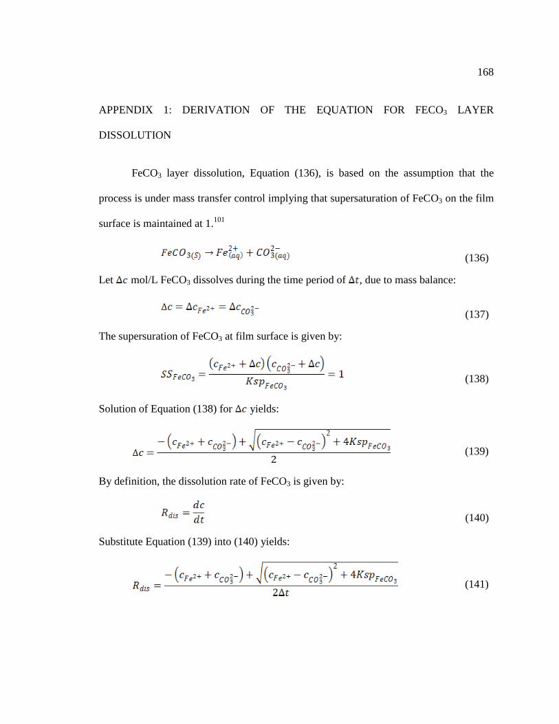
168 APPENDIX 1: DERIVATION OF THE EQUATION FOR FECO3 LAYER
DISSOLUTION
FeCO3 layer dissolution, Equation (136), is based on the assumption that the
process is under mass transfer control implying that supersaturation of FeCO3 on the film
surface is maintained at 1.101
(136)
Let mol/L FeCO3 dissolves during the time period of , due to mass balance:
(137)
The supersuration of FeCO3 at film surface is given by:
(138)
Solution of Equation (138) for yields:
(139)
By definition, the dissolution rate of FeCO3 is given by:
(140)
Substitute Equation (139) into (140) yields:
(141)

169 Where is FeCO3 dissolution rate in mol/(m3.s); :concentration of Fe2+
and CO32- in mol/m3; is supersaturation of FeCO3; is the solubility
limit of FeCO3, is time in sec.
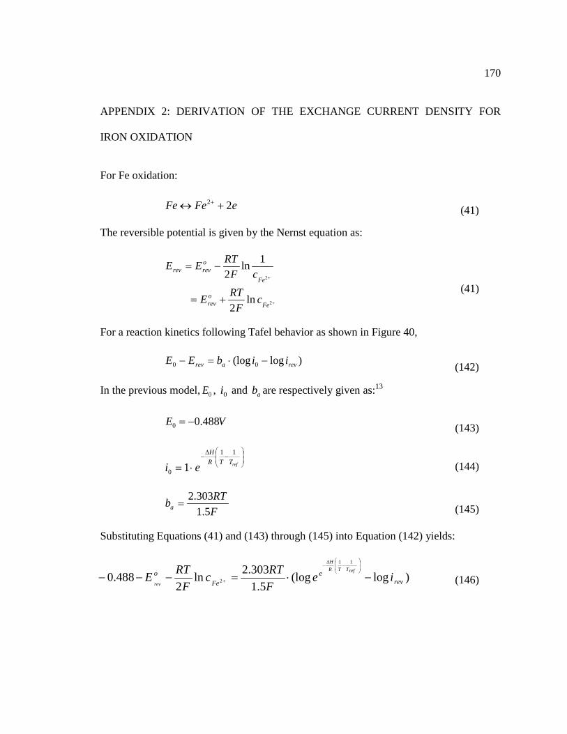
170 APPENDIX 2: DERIVATION OF THE EXCHANGE CURRENT DENSITY FOR
IRON OXIDATION
For Fe oxidation:
eFeFe 22 +↔ +
(41)
The reversible potential is given by the Nernst equation as:
+
+
+=
−=
2
2
ln2
1ln2
Feorev
Fe
orevrev
cF
RTE
cFRTEE
(41)
For a reaction kinetics following Tafel behavior as shown in Figure 40,
)log(log 00 revarev iibEE −⋅=− (142)
In the previous model, 0E , 0i and ab are respectively given as:13
VE 488.00 −= (143)
−
∆−
⋅= refTTRH
ei11
0 1 (144)
FRTba 5.1
303.2= (145)
Substituting Equations (41) and (143) through (145) into Equation (142) yields:
)log(log5.1
303.2ln2
488.011
2 reve
Feo ie
FRTc
FRTE
refTTRH
rev−⋅=−−−
−
∆−
+ (146)

171
)log(log303.2
5.1303.2
ln2
488.0 112
reveFe
o
ie
FRT
cF
RTErefTTR
H
rev
−⋅=−−−
−
∆−+
(147)
rev
Feo
ie
FRT
cF
RTErefTTR
H
rev
lnln
5.1
ln2
488.0 112
−=−−−
−
∆−+
(148)
( )rev
refFe
o
iTTR
Hc
FRT
Erev ln11ln
25.1
5.1
488.02 −
−
∆−=−
+−+
(149)
−
∆−+=
+ref
rev TTRHc
Ti
Fe
11ln6.835ln 75.02
(150)
−
∆−
⋅⋅=+
ref
Fe
TTRH
Trev ecei
11
75.06.835
2
(151)
Where revE : reversible potential of Fe oxidation, V; orevE : reversible potential of Fe
oxidation at standard conditions, -0.44V vs. SHE; R : universal gas constant, 8.3145
J/mol.K; T : temperature, Kelvin; F : Faraday constant, 96485C/mol; +2Fec : surface
concentration, mol/L; 0E : a reference potential, -0.488V; 0i : anodic current density at the
reference potential, A/m2; revi : exchange current density at the reversible potential, A/m2;
H∆ : activation energy for Fe oxidation, 37.5kJ/mol; ab : anodic Tafel slope for Fe
oxidation; refT : reference temperature for Fe oxidation, K.
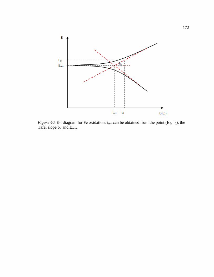
172
Figure 40. E-i diagram for Fe oxidation. irev can be obtained from the point (E0, i0), the Tafel slope ba and Erev.

173 APPENDIX 3: DERIVATION OF THE EXCHANGE CURRENT DENSITY FOR H+
REDUCTION
For H+ reduction,
221 HeH ↔++
(152)
The reversible potential is given by the Nernst equation as:
( )+
+
⋅=
−=
HH
H
Horevrev
cpF
RTcp
FRTEE
5.0
5.0
2
2
ln
ln
(153)
For a cathodic reaction kinetics following Tafel behavior as shown in Figure 41:
crev
rev bii
EE=
−−
0
0
loglog
(154)
0E , 0i and cb have been respectively given as:
( )+= HcF
RTE ln0
(155)
−
∆−
⋅= refTTRH
ref eii11
0
(156)
FRTbc 5.0
303.2= (157)
Substituting Equations (153) and (155) through (157) and into Equation (154)
yields:

174
( ) ( )FRT
ii
cF
RTcpF
RT
rev
HHH
5.0303.2
loglog
lnln
0
5.02
=−
−⋅ ++
(158)
( ) ( )( ) ( ) 2
lnlnlnln
0
5.02 =
−
−⋅ ++
iiccp
rev
HHH
(159)
=
⋅
+
+
0
5.0
ln2ln 2
ii
ccp
rev
H
HH
(160)
2
0
5.02
=
iip rev
H
(161)
25.00 2Hrev pii ⋅=
(162)
Where revE : reversible potential of H+ reduction, V; orevE : reversible potential of H+
reduction at standard conditions, 0V vs. SHE; R : universal gas constant, 8.3145
J/mol.K; T : temperature, Kelvin; F : Faraday constant, 96485C/mol; +Hc : surface
concentration of H+, mol/L; 2Hp : paritial pressure of Hydrogen gas at metal surface, Pa;
0E : a reference potential; 0i : anodic current density at the reference potential, A/m2; revi :
exchange current density at the reversible potential, A/m2; H∆ : activation energy for Fe
oxidation, 37.5kJ/mol; cb : cathodic Tafel slope for Fe oxidation; refT : reference
temperature for Fe oxidation, K.
Note: although this derivation is demonstrated for H+ reduction, it can be shown that
similar expressions can be obtained for H2CO3 reduction and HAc reduction due to
thermodynamic equivalence of these reactions.
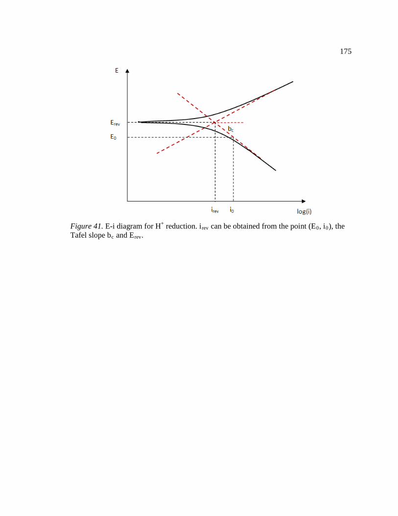
175
Figure 41. E-i diagram for H+ reduction. irev can be obtained from the point (E0, i0), the Tafel slope bc and Erev
.

176 APPENDIX 4: DETERMINATION OF THE ENVIRONMENTAL PARAMETERS
AFFECTING PSEUDO-PASSIVE CURRENT DENSITY OF CARBON STEEL BY
CYCLIC POLARIZATION TECHNIQUE
A4.1 Test Procedure and Test Matrix
In these experiments, cyclic polarization technique was utilized to measure the
pseudo-passive current density under various combinations of pH, temperature and
chloride concentration. The test procedure is given by ASTM G61-1998103 and a brief
description of the procedure is presented here.
Prepare the solution, and raise the temperature to the desired level.
Purge solution with high purity CO2 gas (purity>99.99%) for at least 1 hour. Then
adjust solution pH to the appropriate value with HCl or NaCO3 solution.
Wet grind cylindrical coupon made from carbon steel C1018 using 150-grit sand
paper followed by 600-grit sand paper made of silicon carbide. Rinse the coupon
with deionized water and iso-propanol, respectively.
Dry the coupon in cool air. Set the coupon in still in the solution for at least 1
hour before the test.
Anodically polarize the coupon at the rate of 0.6V/hour starting from the open
circuit potential, until current reaches 54 mA or potential reaches the level at
which water oxidation occurs, and then cathodically polarize back towards the
open circuit potential.

177
The test is terminated whenever open circuit potential is reached or hysteresis
loop of the polarization curve is closed. The test conditions are listed in Table 6.
Table 6. Test conditions for cyclic polarization test Test method cyclic polarization
Test equipment Glass cell
Test specimen C1018
Total Pressure 1bar
Temperature 60 ºC and 80 ºC
pH 7 and 8
Velocity stagnant
NaCl concentration 0.2 mol/L and 2 mol/L
Sweep rate 0.1667mV/s (ASTM G61)
To facilitate the analysis of test results and obtain quantitative information for the
tested parameters, the factorial experiment design technique was used to formulate the
test matrix.104 A 23 test matrix was designed, where two extreme levels of values were
assigned to each parameter. All possible combinations of parameters were tested, which
gives a total number of 8 tests. The test matrix is listed in Table 7.

178
Table 7. Test matrix for factorial design experiments Test number pH Temp/°C NaCl/ mol/L
1 7 60 0.2
2 8 60 0.2
3 7 80 0.2
4 8 80 0.2
5 7 60 2
6 8 60 2
7 7 80 2
8 8 80 2
A4.2 Test Results
Figure 42 through Figure 49 show the cyclic polarization curves obtained for each
condition.
-0.8
-0.6
-0.4
-0.2
0
0.2
0.4
0.6
0.8
0 20 40 60 80 100Current density/A/m2
Pot
entia
l vs.
Ag/
AgC
l/ V
2
Active
pass
ive
tranp
assiv
e
Ipass
Etrans
-0.8
-0.6
-0.4
-0.2
0
0.2
0.4
0.6
0.8
0 20 40 60 80 100Current density/A/m2
Pot
entia
l vs.
Ag/
AgC
l/ V
2
-0.8
-0.6
-0.4
-0.2
0
0.2
0.4
0.6
0.8
0 20 40 60 80 100Current density/A/m2
Pot
entia
l vs.
Ag/
AgC
l/ V
-0.8
-0.6
-0.4
-0.2
0
0.2
0.4
0.6
0.8
0 20 40 60 80 100Current density/A/m2
Pot
entia
l vs.
Ag/
AgC
l/ V
-0.8
-0.6
-0.4
-0.2
0
0.2
0.4
0.6
0.8
0 20 40 60 80 100Current density/A/m2
Pot
entia
l vs.
Ag/
AgC
l/ V
2
Active
pass
ive
tranp
assiv
e
Ipass
Etrans
Figure 42. Cyclic polarization curve of C1018. Test conditions: T=60°C, pH=7, NaCl=0.2 mol/L.
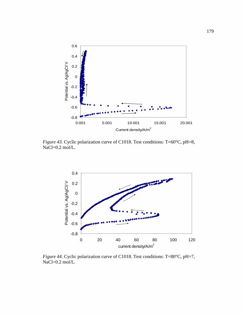
179
-0.8
-0.6
-0.4
-0.2
0
0.2
0.4
0.6
0.001 5.001 10.001 15.001 20.001
Current density/A/m2
Pote
ntia
l vs.
Ag/
AgC
l/ V
-0.8
-0.6
-0.4
-0.2
0
0.2
0.4
0.6
0.001 5.001 10.001 15.001 20.001
Current density/A/m2
Pote
ntia
l vs.
Ag/
AgC
l/ V
Figure 43. Cyclic polarization curve of C1018. Test conditions: T=60°C, pH=8, NaCl=0.2 mol/L.
-0.8
-0.6
-0.4
-0.2
0
0.2
0.4
0 20 40 60 80 100 120current density/A/m2
Pot
entia
l vs.
Ag/
AgC
l/ V
-0.8
-0.6
-0.4
-0.2
0
0.2
0.4
0 20 40 60 80 100 120current density/A/m2
Pot
entia
l vs.
Ag/
AgC
l/ V
Figure 44. Cyclic polarization curve of C1018. Test conditions: T=80°C, pH=7, NaCl=0.2 mol/L.

180
-1
-0.8
-0.6
-0.4
-0.2
0
0.2
0.4
0.6
0 0.5 1 1.5 2 2.5 3 3.5
Current density/A/m2
Pot
entia
l vs.
Ag/
AgC
l/ V
-1
-0.8
-0.6
-0.4
-0.2
0
0.2
0.4
0.6
0 0.5 1 1.5 2 2.5 3 3.5
Current density/A/m2
Pot
entia
l vs.
Ag/
AgC
l/ V
Figure 45. Cyclic polarization curve of C1018. Test conditions: T=80°C, pH=8, NaCl=0.2 mol/L.
-0.8-0.7-0.6-0.5-0.4-0.3-0.2-0.1
00.1
0 10 20 30 40 50 60
Current density/A/m2
Pot
entia
l vs.
Ag/
AgC
l/ V
-0.8-0.7-0.6-0.5-0.4-0.3-0.2-0.1
00.1
0 10 20 30 40 50 60
Current density/A/m2
Pot
entia
l vs.
Ag/
AgC
l/ V
Figure 46. Cyclic polarization curve of C1018. Test conditions: T=60°C, pH=7, NaCl=2 mol/L.
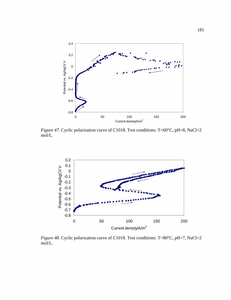
181
-0.8
-0.6
-0.4
-0.2
0
0.2
0.4
0 50 100 150 200Current density/A/m2
Pot
entia
l vs.
Ag/
AgC
l/ V
-0.8
-0.6
-0.4
-0.2
0
0.2
0.4
0 50 100 150 200Current density/A/m2
Pot
entia
l vs.
Ag/
AgC
l/ V
Figure 47. Cyclic polarization curve of C1018. Test conditions: T=60°C, pH=8, NaCl=2 mol/L.
-0.8-0.7-0.6-0.5-0.4-0.3-0.2-0.1
00.10.2
0 50 100 150 200
Current density/A/m2
Pot
entia
l vs.
Ag/
AgC
l/ V
-0.8-0.7-0.6-0.5-0.4-0.3-0.2-0.1
00.10.2
0 50 100 150 200
Current density/A/m2
Pot
entia
l vs.
Ag/
AgC
l/ V
Figure 48. Cyclic polarization curve of C1018. Test conditions: T=80°C, pH=7, NaCl=2 mol/L.

182
-0.9
-0.8
-0.7
-0.6
-0.5
-0.4
-0.3
-0.2
-0.1
0
0 5 10 15 20 25 30 35
Current density/A/m2
Pot
entia
l vs.
Ag/
AgC
l/ V
-0.9
-0.8
-0.7
-0.6
-0.5
-0.4
-0.3
-0.2
-0.1
0
0 5 10 15 20 25 30 35
Current density/A/m2
Pot
entia
l vs.
Ag/
AgC
l/ V
Figure 49. Cyclic polarization curve of C1018. Test conditions: T=80°C, pH=8, NaCl=2 mol/L.
The pseudo-passive current density is summarized in Table 8.
Table 8. Summary of the results for cyclic polarization tests
Test number pH Temp/ °C NaCl/ mol/L Passive current
density/A/m2
1 7 60 0.2 8~9
2 8 60 0.2 0.03~0.7
3 7 80 0.2 ~33
4 8 80 0.2 0.02~0.1
5 7 60 2 ~2
6 8 60 2 0.2~0.5
7 7 80 2 ~50
8 8 80 2 0.03~0.2
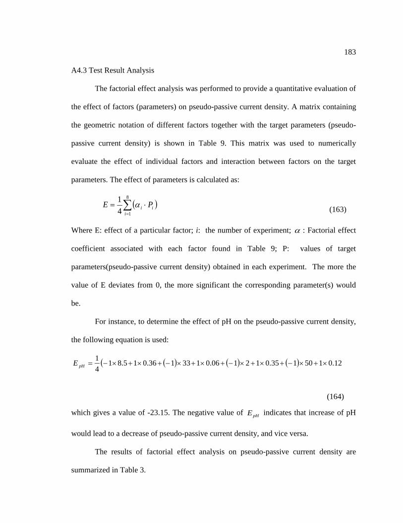
183 A4.3 Test Result Analysis
The factorial effect analysis was performed to provide a quantitative evaluation of
the effect of factors (parameters) on pseudo-passive current density. A matrix containing
the geometric notation of different factors together with the target parameters (pseudo-
passive current density) is shown in Table 9. This matrix was used to numerically
evaluate the effect of individual factors and interaction between factors on the target
parameters. The effect of parameters is calculated as:
( )∑=
⋅=8
141
iii PE α
(163)
Where E: effect of a particular factor; i: the number of experiment; α : Factorial effect
coefficient associated with each factor found in Table 9; P: values of target
parameters(pseudo-passive current density) obtained in each experiment. The more the
value of E deviates from 0, the more significant the corresponding parameter(s) would
be.
For instance, to determine the effect of pH on the pseudo-passive current density,
the following equation is used:
( ) ( ) ( )( 12.0150135.012106.0133136.015.8141
×+×−+×+×−+×+×−+×+×−=pHE
(164)
which gives a value of -23.15. The negative value of pHE indicates that increase of pH
would lead to a decrease of pseudo-passive current density, and vice versa.
The results of factorial effect analysis on pseudo-passive current density are
summarized in Table 3.

184 Table 9. Matrix used for performing factorial effect analysis
Run Factorial Effect Coefficient Passive current
density/A/m2 pH T pH & T Cl- pH & Cl- T & Cl- pH&T&Cl-
1 -1 -1 1 -1 1 1 -1 8.5
2 1 -1 -1 -1 -1 1 1 0.36
3 -1 1 -1 -1 1 -1 1 33
4 1 1 1 -1 -1 -1 -1 0.06
5 -1 -1 1 1 -1 -1 1 2
6 1 -1 -1 1 1 -1 -1 0.35
7 -1 1 -1 1 -1 1 -1 50
8 1 1 1 1 1 1 1 0.12
Table 3. Effect of factors on passive current density Factors Effect
pH -23.15
T 17.99
pH & T -18.26
[Cl-] 2.64
pH & [Cl-] -2.61
T & [Cl-] 5.89
pH & T & [Cl-] -5.86

185 APPENDIX 5: MODELING PSEUDO-PASSIVE CURRENT DENSITY OF CARBON
STEEL IN CO2 ENVIRONMENT BASED ON POINT DEFECT MODEL
A5.1 Introduction
The Point Defect Model is considered to be one of the most successful
mechanistic models describing passivity; it was originally developed by D. Macdonald
and his colleagues beginning in the early 1980s.28-31 The model is based on the
hypothesis that passive current density is governed by the transport of various defects
(vacancies and interstitials) through the passive film. The most important assumptions
made in the Point Defect Model are:
Electric field strength is independent of film thickness. This assumption has been
verified by experimental evidence, as the potential drop across the passive film
was found to be linearly changed with passive film thickness.32
Passive film/solution interface potential is linearly related to pH and applied
potential.
To ease further discussion of this model, a brief introduction on point defects is
given below. A point defect can be defined as “a lattice site which contains an atom, ion
or molecule which would not be present on that site in a perfectly stoichiometric
material”.128 In nature, any real crystals above absolute zero degree (0 K) contain defects.
A point defect can be either a vacancy site or an interstitial site in a crystal structure. The
two most common types of point defect are so-called Schottky and Frenkel defects, as
demonstrated in Figure 50. It can be seen that the Schottky defect contains a pair of

186 cation and anion vacancies, while Frenkel defect is made of a cationic interstitial ion
accompanied by a corresponding cation vacancy. Some characteristics of point defects
related to the Point Defect Model are listed below.
Interstitial ions exist in significant amount only when the size of the cation is
much smaller than the anion.
Ions situated at normal sites are electronically neutral; however, vacancies are
negatively or positively charged to balance the surrounding ions.
For a Schottky defect, a cation vacancy must be accompanied by certain numbers
of anion vacancy to maintain overall electro-neutrality of the crystal.

187 Figure 50. Illustration of the Schottky(a) and Frenkel(b) defects by Gao.128
A5.2 Model Development
A Point Defect Model for CO2 environments proposed by O. R. Camacho et al. is
schematically illustrated in Figure 51.38 A bi-layer structure was suggested in this model,
which includes a passive film (barrier layer) and an outer layer (mainly composed of
FeCO3). A total of 9 reactions were proposed to take place at 3 interfaces, metal/passive
film, passive film/outer layer and outer layer/solution. Various vacancies, cation
interstitials and aqueous species are involved in the reactions.

188 Figure 51. Original point defect model for carbon steel.38 Fe: Fe atom on a metal lattice site; FeFe: Fe on Fe site in the oxide; Fei
χ+: iron interstitial in the oxide layer; OO: oxygen ion in the oxide; VFe
χ’= Fe vacancy; VO..= oxygen vacancy; FeГ+: metallic species in
solution; FeOχ/2: oxide barrier layer; FeCO3: precipitated outer layer; ki
: reaction rate constant; BL: oxide barrier layer; OL: outer layer.
In this work, modifications were made to this model for proper coupling of the
Point Defect Model with the localized corrosion model. The pseudo-passive film
considered in this study is magnetite (FeO+Fe2O3) through which vacancies of Fe3+ and
O2- travels; however, interstitial defects are not taken into account. This is because the
radius of Fe3+ in a crystal (about 0.785 nm) is not significantly smaller than that of O2-
(about 1.25nm).129 It would require a significant amount of energy for Fe3+ to squeeze
into the lattice structure formed by O2- . Hence, it was determined that the interstitial
defects, would not contribute much to the electrical charge-carrying process. Further
simplification was made by excluding the outer layer in the model, which is mainly
composed of FeCO3 in a carbon steel/CO2 system. This is because the potential
distribution in the solution (including that within FeCO3 layer) can be obtained by
solving the Laplace equation, which allows for direct determination of potential on the
pseudo-passive surface. Therefore, potential gradient across FeCO3 layer is not required
in this particular model. Figure 52 shows schematic of the revised model proposed in this
study.
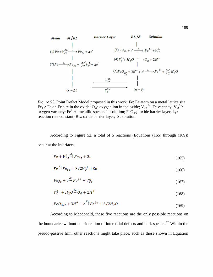
189
Figure 52. Point Defect Model proposed in this work. Fe: Fe atom on a metal lattice site; FeFe: Fe on Fe site in the oxide; OO: oxygen ion in the oxide; VFe
3-: Fe vacancy; VO2+:
oxygen vacancy; Fe2++: metallic species in solution; FeO3/2: oxide barrier layer; ki
: reaction rate constant; BL: oxide barrier layer; S: solution.
According to Figure 52, a total of 5 reactions (Equations (165) through (169))
occur at the interfaces.
(165)
(166)
(167)
(168)
(169)
According to Macdonald, these five reactions are the only possible reactions on
the boundaries without consideration of interstitial defects and bulk species.28 Within the
pseudo-passive film, other reactions might take place, such as those shown in Equation

190 (170) and (171);128 however, electrons are not involved in these reactions and so the
existence of these reactions would not affect the current traveling within the film.
(170)
(171)
It has been argued that Reactions (165), (167) and (168) are lattice conservative,28
which means that these reactions would not lead to the movement of boundaries, but are
dedicated to transfer of charge. Reactions (166) and (169), however, are considered to be
responsible for pseudo-passive film growth and dissolution, respectively. This argument
deserves further discussion. It can be seen that Reactions (165), (167) and (168) involve
the generation of a species ( in reaction (165), in reaction (167) and in
reaction (168)) at the expense of consumption of another specie( in reaction
(165), in reaction (167) and in reaction (168)). It can be imagined that
consumption/loss of the species on the boundaries of pseudo-passive film could lead to
neighboring ions with a coordination number only one less than that in the bulk;
therefore, the site of consumption can be viewed as a vacancy site, that will be
replenished by the upcoming ions, while site of generation will be occupied by upcoming
vacancies. Hence, at the steady state, boundaries will be maintained due to continuous
consumption/supplement of ions or vacancies on the boundaries. As to Reaction (166), a
cationic ion( ) and a vacancy( ) are generated for every one iron atom in the base
metal. In other words, this reaction generates new pseudo-passive film without
consuming itself. Therefore, this reaction would lead to pseudo-passive film growth.

191
Details are given below for equation derivation of pseudo-passive current density
based on the model presented in Figure 52.
At steady state, electron fluxes can be expressed in terms of fluxes of vacancies
for Reactions (165) through (168), respectively. No vacancies are involved in reaction
(169); therefore, electron flux is expressed in terms of of H+ concentration.
For Reaction (165):
(172)
For Reaction (166):
(173)
For Reaction (167):
(174)
For Reaction (168):
(175)
For Reaction (169):
(176)
Total electron flux is gained by summing up electron fluxes in all reactions:
(177)
Current density is related to electron flux as:
(178)
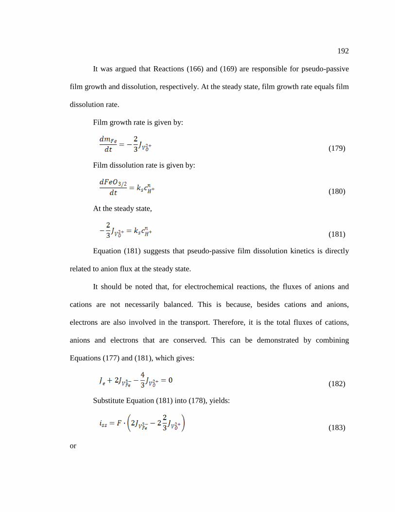
192
It was argued that Reactions (166) and (169) are responsible for pseudo-passive
film growth and dissolution, respectively. At the steady state, film growth rate equals film
dissolution rate.
Film growth rate is given by:
(179)
Film dissolution rate is given by:
(180)
At the steady state,
(181)
Equation (181) suggests that pseudo-passive film dissolution kinetics is directly
related to anion flux at the steady state.
It should be noted that, for electrochemical reactions, the fluxes of anions and
cations are not necessarily balanced. This is because, besides cations and anions,
electrons are also involved in the transport. Therefore, it is the total fluxes of cations,
anions and electrons that are conserved. This can be demonstrated by combining
Equations (177) and (181), which gives:
(182)
Substitute Equation (181) into (178), yields:
(183)
or

193
(184)
Equation (183) indicates that the pseudo-passive current density is attributed to
the movement of both cations and anions. Equation (184) suggests that the pseudo-
passive current density is a result of competition between cation flux and passive film
dissolution. Because anion flux is at the same rate of film dissolution (Equation (181)), it
can be readily deduced that cation movement must be dominant in the transport process
to maintain a steady pseudo-passive film.
Flux of Fe3+ vacancy can be calculated by considering Reaction (167) which is
the only reaction where Fe3+ vacancy is involved on the pseudo-passive film/solution
boundary. The total flux of Fe3+ vacancy at steady state can be calculated as:
(185)
Substituting Equation (185) into (184), gives:
(186)
The rate constant of an electrochemical reaction is given by:28
(187)
Apply Equation (187) to reactions (167) and (169), yield:
(188)
(189)
Let , Equations (188) and (189) can be simplified as:
(190)

194
(191)
Assuming that the potential at pseudo-passive film/solution interface is linearly
related to pH and metal potential (temperature has been found to be a minor factor):28
(192)
Substituting Equation (192) into Equations (190) and (191), yields:
(193)
(194)
Where
(195)
(196)
Substituting Equation (193) and (194) into Equation (186), the pseudo-passive
current density can be calculated as:
(197)
The previous work performed by Macdonald et al. has shown that:38,130
The only parameters to be determined are x and y.
By incorporating Equation (197) into the localized corrosion model and by
adjusting the values of x and y, the model is calibrated against the measured galvanic
current density values obtained in an artificial pit test,105 which yields x=-0.01 and
y=0.01. The equation for pseudo-passive current density is then given by:
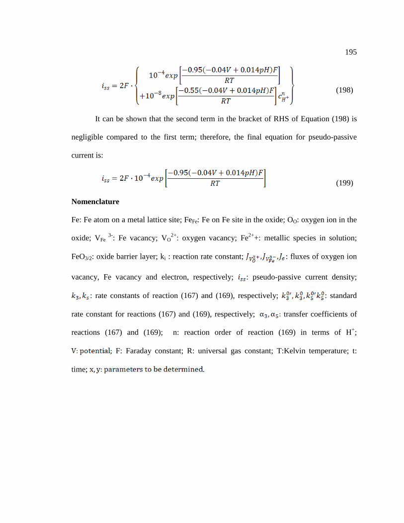
195
(198)
It can be shown that the second term in the bracket of RHS of Equation (198) is
negligible compared to the first term; therefore, the final equation for pseudo-passive
current is:
(199)
Nomenclature
Fe: Fe atom on a metal lattice site; FeFe: Fe on Fe site in the oxide; OO: oxygen ion in the
oxide; VFe 3-: Fe vacancy; VO
2+: oxygen vacancy; Fe2++: metallic species in solution;
FeO3/2: oxide barrier layer; ki : reaction rate constant; : fluxes of oxygen ion
vacancy, Fe vacancy and electron, respectively; : pseudo-passive current density;
: rate constants of reaction (167) and (169), respectively; : standard
rate constant for reactions (167) and (169), respectively; transfer coefficients of
reactions (167) and (169); n: reaction order of reaction (169) in terms of H+;
F: Faraday constant; R: universal gas constant; T:Kelvin temperature; t:
time; .
196
APPENDIX 6: OPEN SOURCE MODEL OF UNIFORM CO2/H2S CORROSION
A6.1 Introduction
Carbon steel is the most commonly used engineering structural material the in oil
and gas industry. In such environments, various aggressive species, such as CO2, H2S and
organic acids tend to attack pipelines made from carbon steel. In the past few decades,
uniform corrosion of carbon steel in oil and gas pipelines has been extensively studied,
leading to sizable publications targeting many key aspects of uniform corrosion.
Although not completely understood, most steps associated with CO2 corrosion
mechanisms are now believed to be clear. H2S corrosion is still subject to ongoing
investigation, but initial study has shed some light on the understanding of uniform
corrosion mechanisms.132 With information available from the open literature, it is now
possible to build a mechanistic model to predict uniform corrosion rates in order to assist
with the understanding of the corrosion process. In fact, a number of models for CO2
corrosion in wells and pipelines have been developed in recent years, as summarized by
Nyborg.3 However, the availability of most of these models to the public is largely
limited due to their proprietary nature. In addition, a large scatter in the prediction is not
uncommon resulting from different theories, assumptions and modeling strategies. Due to
the lack of transparency of the code behind the models, it is difficult for users to make a
sound judgment as to which one is more reliable. It can be imagined that, as the corrosion
process becomes increasingly complex, larger discrepancies may be expected from
various models. This section of work is aimed at providing the corrosion community with
a free mechanistic model for internal corrosion prediction of carbon steel pipelines

197 particularly related to oil and gas industry. Strongly rooted in theories, this model can
offer trustworthy predictions for a wide range of conditions, as will be shown in the
following sections. The model, named FREECORP, was developed exclusively based on
public information. All the information related to the model, including theories,
assumptions and limitations, is available to the users and can be accessed through
http://www.corrosioncenter.ohiou.edu/freecorp. In addition, the source code is open and
shared. With open source code, the model can be improved and expanded by adding new
modules or modifying existing modules. By doing so, model capability can be extended
to accommodate a wider range of environments.
As already mentioned in a previous publications, the motivation of offering this
model to the corrosion community is:16
To elevate the level of understanding and the prediction capability of mild steel
corrosion as related to the oil and gas industry.
To ensure that the best available science and technology is available to corrosion
engineers, and implemented using a transparent approach that is open for further
development and improvement.
To increase the level of involvement of the broader corrosion community in
developing better and more flexible tools suited for their intended purposes, an
approach which will hopefully be mimicked in the future in other fields of corrosion.
To fulfill one of the key missions of the Institute for Corrosion and Multiphase
Technology and Ohio University as a public institution, which is to educate the wider
professional community and extend its reach beyond the pool of the current research

198
sponsors in order to enable more effective dissemination of the already published
knowledge and technology.
This model is able to predict a uniform corrosion rate for carbon steel under attack
by CO2, H2S, HAc and/or O2. To facilitate the understanding of corrosion mechanisms,
additional information is given apart from corrosion rate. For instance, the contribution of
each corrosive species to the overall corrosion rate is quantified as a percentile. An Evans
diagram is provided for CO2/HAc/O2 corrosion where polarization curves are shown for
individual electrochemical reactions as well as total anodic and cathodic reactions. For
H2S corrosion, the H2S concentration profile across the mackinawite layers and the liquid
boundary layer is illustrated in place of an Evans diagram. It was determined that the H2S
concentration profile would be more informative and useful, since the H2S corrosion
model is based on the assumption of mass transfer control. The effect of FeCO3 and FeS
is simulated using empirical correlations in order to achieve a better prediction.
In the following sections, the main theories related to uniform corrosion caused
by CO2, H2S, HAc and/or O2 are briefly reviewed, followed by a description of the
implementation of these theories into the model. Model verification and parametric study
are then presented. In the final section, limitations of the current version of the model are
described and directions for future development are pointed out.
A6.2 Theories of the Model
Although many publications are referenced during model development, 3 key
papers are used as the theoretical basis of this model. These are: the paper by Nešić,
Postelthwaite and Olsen for CO2 corrosion131, that by George, Nešić and de Waard for

199 HAc corrosion96 and that by Sun and Nešić for H2S corrosion132. CO2 and HAc corrosion
are electrochemical processes involving water chemistry, electrochemistry and mass
transport. Those effects have been previously discussed in Chapter 4 above and will not
be replicated here.
Compared to CO2 corrosion, H2S corrosion is much less understood. Even though
abundant experimental data for H2S corrosion have been presented in the open literature,
discrepancies and contradictions are often seen in the literature. At present, the topic of
H2S corrosion mechanism is still subject to much debate. From the experimental results,
H2S corrosion seems to manifest itself as a fast surface reaction (either chemical or
electrochemical) followed by massive FeS layer growth.132 An FeS layer is always
present on a corroding steel surface in an H2S-containing environment, causing
substantial reduction of the general corrosion rate. Although the current level of
knowledge does not grant a solid mechanism that is consistent with all experimental
observations and agreed upon by all researchers, this model employs a mechanism
proposed by Sun et al., 132 that is considered to be plausible and supported by many
experimental results. According to this theory, H2S is initially absorbed onto the steel
surface and immediately reacts with iron to form a very thin (<<1 mµ ), dense and
protective non-stoichiometric iron sulfide film – mackinawite. Due to its compactness,
this film acts as a solid-state diffusion barrier for species involved in the corrosion
process and leads to a significant and rapid reduction of the corrosion rate. Although
slow, diffusion of the corrosive species through this mackinawite film does not
completely cease, and the continuing corrosion at the steel surface continues to generate
200 more mackinawite. As this process proceeds, the internal stress in the mackinawite film
is built up due to epitaxial stresses and the Pilling-Bedford ratio (large volume ratio of the
mackinawite to iron). These stresses lead to microcracking and eventually delamination
of the mackinawite film. A cyclic process of growth, cracking and delaminating of
mackinawite eventually leads to the formation of an outer mackinawite layer that is
thicker, more porous and less protective.
Considering the fact that the inner and outer FeS layers are always present in H2S
corrosion, Sun et al. assume that H2S corrosion is under mass transfer control.132
Corrosion rate is limited by the mass transfer of corrosive species, such as H2S, CO2, H+,
HAc, etc., through the FeS layers on steel surface.
In reality, H2S corrosion can be complicated by a number of factors. For instance,
given enough time, the mackinawite film might transform into other forms of sulfides
such as pyrrhotite. In addition, pyrrhotite might precipitate from the solution to form an
additional solid layer and further increase mass transfer resistance. In the presence of
high-concentration H2S and oxygen, elemental sulfur might form in the pipelines and
induce localized corrosion. These effects are not included in the present version of the
model.138
A6.3 Mathematical Model
The FREECORP model is a simplified version of the model presented in Chapter
4 for uniform corrosion (MULTICORP V5). The CO2/HAc corrosion model is a simple
electrochemical model in which corrosion rate is determined based on the fact that the
total anodic current is balanced by the total cathodic current. The H2S corrosion rate is

201 calculated based on the assumption of mass transfer limiting, which implies that
corrosion rate is determined by the diffusion rates of corrosive species. Unlike
MULTICORP, where mass transfer of species is obtained by solving complex partial
differential equations, in FREECORP it is calculated by the concept of a mass transfer
coefficient involving a simple empirical correlation. For CO2 corrosion, pure charge
transfer and mass transfer/chemical reaction-limiting current density are calculated for
each cathodic reaction independently, which are then coupled together to give an
integrated scheme of the electrochemical reaction kinetics. This section details the
mathematical description of the model.
A6.3.1 CO2/HAc Corrosion
CO2/HAc corrosion rate is calculated through the determination of individual
electrochemical reaction rates involved in the corrosion process. The electrochemical
reactions that are taken into consideration in this model include: oxidation of iron,
reduction of hydrogen ion, direct reduction of carbonic acid, direct reduction of acetic
acid, reduction of water and reduction of oxygen.
A6.3.1.1 Anodic Reaction
Oxidation of iron is the only anodic reaction considered in this model.
eFeFe 22 +→ + (78)
Reaction (78) is a charge transfer control process within the potential range of
interest. The current density of this reaction can be calculated using the Tafel equation
and is previously given in Table 1. Table 1 presents equations used calculate the charge

202 transfer current density of major electrochemical reactions involved in CO2/HAc
corrosion. In the following text of section 5.3.1, unless otherwise stated, the charge
transfer current density calculation refers to the corresponding equation shown in Table
1.
A6.3.1.2 Cathodic Reactions
Reduction of hydrogen ion
H+ reduction is the primary cathodic reaction in a CO2 system with pH less than 5.
222 HeH →+ −+ (79)
The current density for reduction of hydrogen ion consists of two components:
charge transfer limiting and mass transfer limiting. Total current density is calculated
using a harmonic mean:
+++
+=H
dHaH iii lim,,
111 (200)
Where +Hi : total current density of H+ reduction, A/m2; +Hai ,: charge transfer current
density of H+ reduction, A/m2; dHi +lim,
: mass transfer limiting current density of H+
reduction, A/m2.
The mass transfer limiting current density is related to bulk concentration of H+
as:
FeSFeCOHHmd
H Fcki ηη3,lim, +++ = (201)
Where +Hmk ,: H+ mass transfer coefficient, m/s; +Hc : bulk concentration of H+, mol/m3;
FeSFeCO ηη ,3
: scale factor related to iron carbonate and iron sulfide film, respectively.
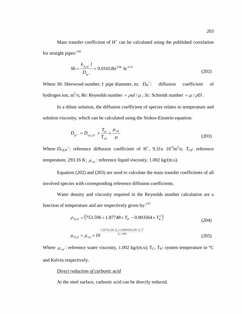
203
Mass transfer coefficient of H+ can be calculated using the published correlation
for straight pipes:136
33.086.0, Re0165.0 ScD
lkSh
H
Hm ==+
+
(202)
Where Sh: Sherwood number; l: pipe diameter, m; DH+: diffusion coefficient of
hydrogen ion, m2/s; Re: Reynolds number µρ /ul= ; Sc: Schmidt number Dρµ /= .
In a dilute solution, the diffusion coefficient of species relates to temperature and
solution viscosity, which can be calculated using the Stokes-Einstein equation:
µµ ref
ref
KHrefH T
TDD ××= ++ , (203)
Where Dref,H+: reference diffusion coefficient of H+, 9.31x 10⁻⁹m2/s; Tref: reference
temperature, 293.16 K; refµ : reference liquid viscosity, 1.002 kg/(m.s).
Equation (202) and (203) are used to calculate the mass transfer coefficients of all
involved species with corresponding reference diffusion coefficients.
Water density and viscosity required in the Reynolds number calculation are a
function of temperature and are respectively given by:137
( )2003564.087748.1596.7532 KKOH TT ×−×+=ρ (204)
105)20(001053.0)20(3272.1 2
210 +
−×−−×
×= C
CCT
TT
refOH µµ (205)
Where refµ : reference water viscosity, 1.002 kg/(m.s); TC, TK: system temperature in °C
and Kelvin respectively.
Direct reduction of carbonic acid
At the steel surface, carbonic acid can be directly reduced.
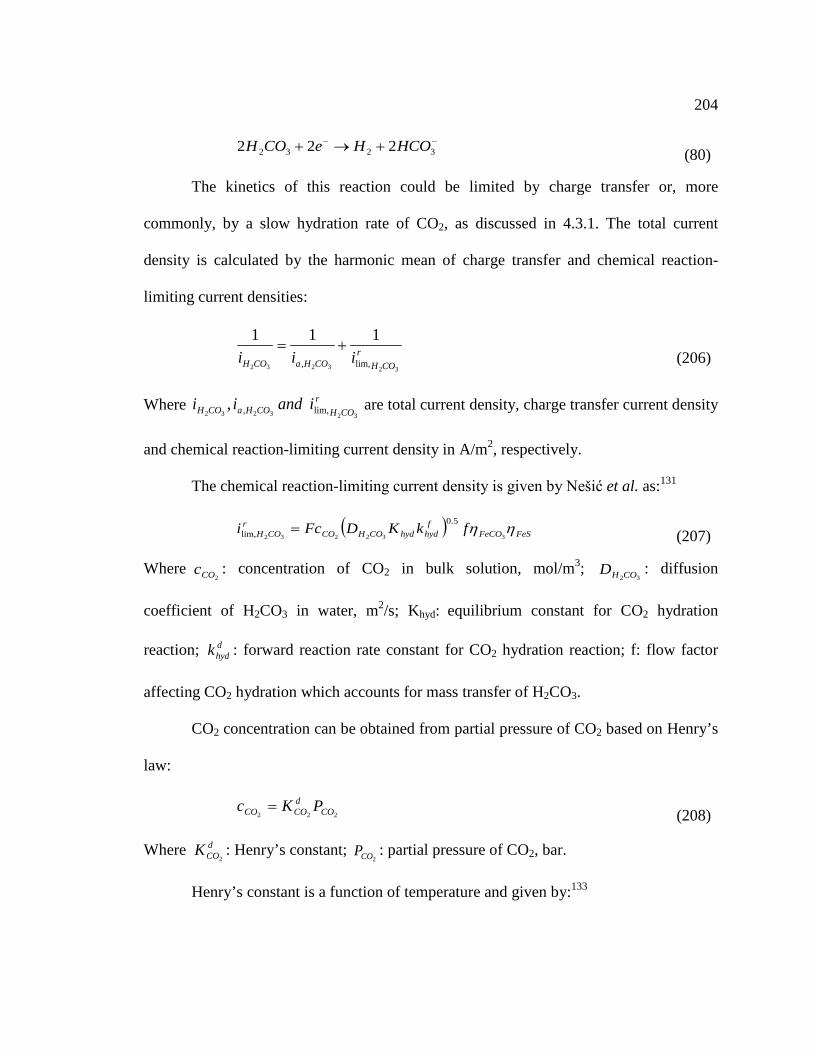
204
−− +→+ 3232 222 HCOHeCOH (80)
The kinetics of this reaction could be limited by charge transfer or, more
commonly, by a slow hydration rate of CO2, as discussed in 4.3.1. The total current
density is calculated by the harmonic mean of charge transfer and chemical reaction-
limiting current densities:
323232 lim,,
111
COHr
COHaCOH iii+=
(206)
Where 323232 lim,,,
COHr
COHaCOH iandii are total current density, charge transfer current density
and chemical reaction-limiting current density in A/m2, respectively.
The chemical reaction-limiting current density is given by Nešić et al. as:131
( ) FeSFeCOf
hydhydCOHCOr
COH fkKDFci ηη332232
5.0lim, = (207)
Where 2COc : concentration of CO2 in bulk solution, mol/m3;
32COHD : diffusion
coefficient of H2CO3 in water, m2/s; Khyd: equilibrium constant for CO2 hydration
reaction; dhydk : forward reaction rate constant for CO2 hydration reaction; f: flow factor
affecting CO2 hydration which accounts for mass transfer of H2CO3.
CO2 concentration can be obtained from partial pressure of CO2 based on Henry’s
law:
222 COdCOCO PKc = (208)
Where dCOK
2: Henry’s constant;
2COP : partial pressure of CO2, bar.
Henry’s constant is a function of temperature and given by:133

205
( )ITTdCO
ffK ×+×−×+− −−
×= 075.01006.81065.527.2 263
210
00258.15.14
(209)
The forward reaction rate constant for CO2 hydration is a function of temperature
and given by:134
KK T
Tf
hydk4.17265log541.11085.329
10−−
= (210)
Flow factor f is given by:135
rm
rm
eef δδ
δδ
/2
/2
11
−
−
−+
= (211)
Where mδ and rδ are defined as mass transfer and reaction layer thickness, respectively,
which can be calculated as:135
32
32
, COHm
COHm k
D=δ (212)
fhyd
hydCOHr k
KD32=δ
(213)
Where 32, COHmk is the mass transfer coefficient of H2CO3 in m/s, which can be obtained
using Equations (202) and (203).
It has been argued that flow factor becomes significant only when thickness of the
mass transfer boundary layer is of the same order as the reaction layer.
Direct reduction of HAc
Acetic acid takes part in the corrosion process in two main ways. Firstly, by
dissociation, it can provide additional sources of H+ to be reduced. Secondly, it can be
directly reduced on the steel surface and further increase the corrosion rate.
206
−− +→+ COOCHHeCOOHCH 323 222 (81)
It has been shown that the current density for direct reduction of HAc could be
limited either by charge transfer or mass transfer.96 The total current density is given by:
HAcd
HAcaHAc iii lim,,
111+= (81)
Where HAc
dHAcaHAc iandii lim,,, are total current density, charge transfer current density and
mass transfer limiting current density of this reaction in A/m2, respectively.
The mass transfer limiting current density of this reaction is given by:
FeSFeCOHAcHAcmd
HAc Fcki ηη3,lim, = (214)
Where HAcmk , : mass transfer coefficient of HAc, m/s; HAcc : bulk concentration of acetic
acid, mol/m3.
Oxygen reduction
Although oxygen is not a common corrosive species in oil and gas pipeline
systems, it could invade the system through inappropriate operation or insufficient de-
oxidation of chemical solutions injected into the system. In order to take into account
oxygen contamination, oxygen reduction is built in the model as well.
Like H+ reduction and HAc reduction, the current density of oxygen reduction
could be limited by either charge transfer or mass transfer. The current density is
therefore calculated as:
222 lim,,
111
Od
OaO iii+= (215)

207 Where
2Oi : total current density of oxygen reduction, A/m2; 2,Oai : charge transfer current
density of oxygen reduction, A/m2; 2
lim,Odi : mass transfer limiting current density of
oxygen reduction, A/m2.
Charge transfer current density is given by Tafel equation:
2
2,0
2210,0,
O
O
bEE
OOa ii−
×= (216)
Where 2,0 Oi : current density of oxygen reduction at a reference point, 0.06A/m2;
2,0 OE :
potential of oxygen reduction at a reference point, 0.5V; 2Ob : Tafel slope of oxygen
reduction.
The reference current density of oxygen reduction is a function of temperature:131
−
∆−
×= refK
O
TTRH
OrefO eii11
,0,0
2
22 (217)
Where 2,0 Orefi : current density of oxygen reduction at a reference temperature, A/m2; Tref:
reference temperature, 298.16K; 2OH∆ : activation energy of oxygen reduction, 10k
J/mol.
Mass transfer-limiting current density is given by:131
FeSFeCOOOmd
O Fcki ηη3222 ,lim, 4= (218)
Where 2,Omk : mass transfer coefficient of oxygen, m/s;
2Oc : bulk concentration of
oxygen, mol/m3.
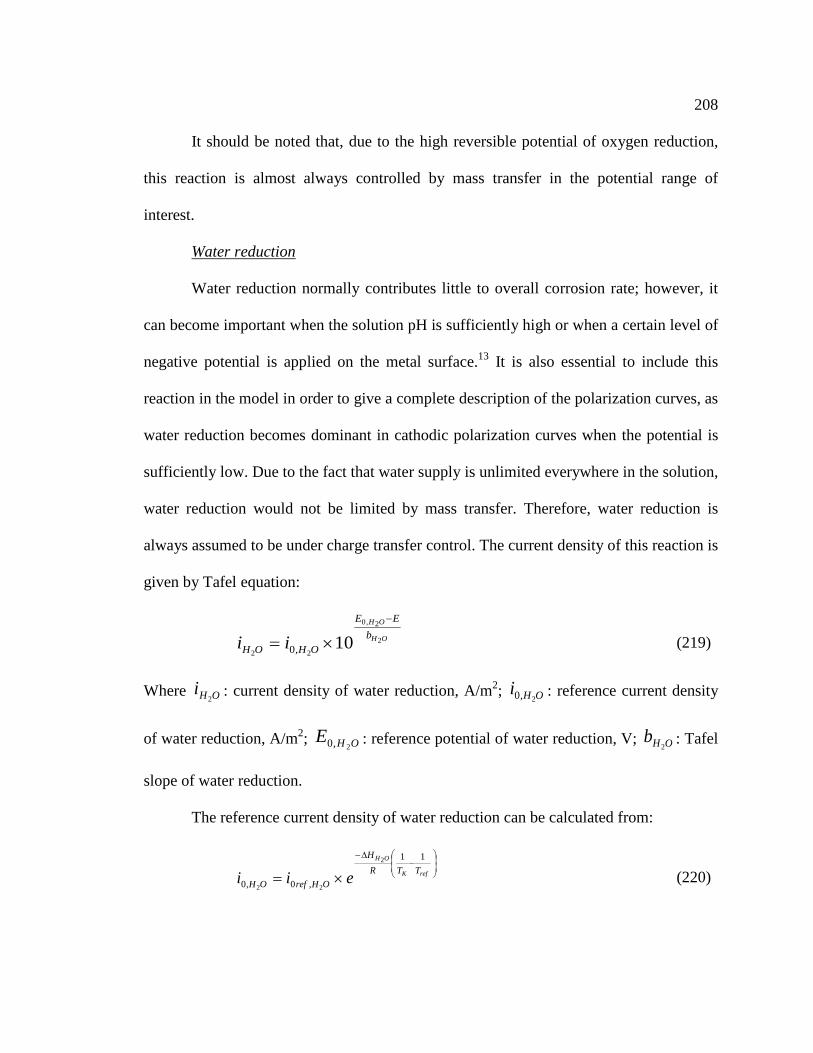
208 It should be noted that, due to the high reversible potential of oxygen reduction,
this reaction is almost always controlled by mass transfer in the potential range of
interest.
Water reduction
Water reduction normally contributes little to overall corrosion rate; however, it
can become important when the solution pH is sufficiently high or when a certain level of
negative potential is applied on the metal surface.13 It is also essential to include this
reaction in the model in order to give a complete description of the polarization curves, as
water reduction becomes dominant in cathodic polarization curves when the potential is
sufficiently low. Due to the fact that water supply is unlimited everywhere in the solution,
water reduction would not be limited by mass transfer. Therefore, water reduction is
always assumed to be under charge transfer control. The current density of this reaction is
given by Tafel equation:
OH
OH
bEE
OHOH ii 2
2,0
2210,0
−
×= (219)
Where OHi 2: current density of water reduction, A/m2; OHi
2,0 : reference current density
of water reduction, A/m2; OHE2,0 : reference potential of water reduction, V; OHb
2: Tafel
slope of water reduction.
The reference current density of water reduction can be calculated from:
−
∆−
×= refK
OH
TTRH
OHrefOH eii11
,0,0
2
22 (220)
209 Where OHrefi
2,0 : reference exchange current density of water reduction, 10-4.45 A/m2;
OHH2
∆ : activation energy of water reduction, 30kJ/mol; Tref: reference temperature,
298.16K.
It has been argued that reduction of water is thermodynamically equivalent to H+
reduction,131 therefore the reference potential and Tafel slope can be calculated in the
same way as those for H+ reduction, as shown in Table 1.
A6.3.1.3 Determination of CO2/HAc Corrosion Rate
The CO2/HAc corrosion rate is determined based on charge balance on the steel
surface. By equating total anodic current density with total cathodic current density, the
unknown corrosion potential can be solved.
∑ ∑=na nc
ca ii1 1
(221)
Where ia, ic: anodic and cathodic current density, respectively, A/m2; ncna, : total
numbers of anodic and cathodic reactions, respectively.
Once corrosion potential is found, current density of individual electrochemical
reactions involved in the corrosion process can be readily calculated. The corrosion rate
can then be determined based on the current density of iron oxidation or the total current
density of cathodic reactions.
a
Fe
Fewa
inF
MiCR
159.1
3652436001000,
=
××××=ρ (222)
210 Where CR: corrosion rate, mm/yr; ia: total anodic current density, A/m2; Mw,Fe: atomic
mass of iron, 55.56g/mol; Feρ : density of iron, 7800g/m3; n: number of moles of
electrons involved in iron oxidation, 2 mole/mol.
A6.3.2 H2S Corrosion
Due to the presence of three layers on steel surface, i.e., a very thin but dense
mackinawite film on steel surface, a porous and often thick outer mackinawite layer and a
liquid boundary layer, H2S corrosion is considered to be under mass transfer control.
Hence, an H2S corrosion rate can be obtained from the total fluxes of the corrosive
species. The flux of individual corrosive species (H2S, H+, H2CO3, HAc, etc.) across
three layers is a function of the mass transfer coefficient and the concentration gradient
within the layer. At steady state, a unique flux is experienced throughout the mass
transfer layers. By equating fluxes in different layers, intermediate concentrations can be
eliminated, which finally leads to an implicit expression for flux related only to the mass
transfer coefficient and the bulk and surface concentrations.
Take H2S as an example. The flux of H2S due to diffusion through the liquid
boundary layer can be calculated as:132
)(2222 ,,, SHoSHbSHmSH cckFlux −= (223)
The flux of H2S due to diffusion through the outer makinawite layer is given
by:132
( )SHiSHoOS
SHSH cc
DFlux
22
2
2 ,, −=δεψ
(224)

211
The flux of H2S due to solid state diffusion through the inner mackinawite film is
given by:132
=
−
SHs
SHiRTB
SHSH cc
eAFlux K
SH
2
2
2
22,
,ln (225)
Where SHFlux2
: flux of H2S, mol/(m2s); SHmk2, : mass transfer coefficient of H2S in
liquid boundary layer, calculated using equation, m/s; SHD2
: diffusion coefficient of H2S
in water, calculated using the Stokes-Einstein correlation (Equation (203)) with reference
diffusion coefficient (Dref,H2S) of H2S of 1.3x10⁻¹⁰m2/s at Tref = 298.16 K and refµ =
1.002kg/(m.s).; ψε , : empirically determined porosity and tortuosity of outer
mackinawite scale, 9.0=ε and 003.0=ψ respectively; osδ : thickness of the outer scale,
m; SHsSHiSHoSHb cccc2222 ,,,, ,,, : concentration of H2S in bulk solution, at outer scale/solution
interface, at inner film/outer scale interface and at steel surface, respectively, mol/m3;
SHSH BA22
, : Arrhenius constants, SHA2
=1.30x10⁻⁴mol/(m2s) and SHB2
=15.5kJ/mol.
Considering steady-state, where the flux of species is constant across these layers,
by equating Equations (223) through (225) to eliminate intermediate concentration, SHoc2,
and SHic2, , the following equation is obtained for the flux of H2S:132
SHs
SHmSH
OSSHSHb
RTB
SHSH c
kDFluxc
eAFlux K
SH
2
22
222
22,
,,
1
ln
+−
=− εψ
δ
(226)
Where SHsc2, is assumed to be 1.0x10⁻⁷ mol/m3.
The thickness of outer mackinawite layer can be calculated as: 132

212
Am
FeS
osos ρ
δ∆
= (227)
Where osm∆ : mass of outer mackinawite layer, kg; FeSρ : density of iron sulfide, kg/m3
and A: surface area of steel, m2.
The mass of the outer mackinawite layer can be calculated based on the scale
retention rate, which is related to the damage of mackinawite layer: 132
tAMSRRm FeSos ∆⋅⋅⋅=∆ (228)
Where SRR: scale retention rate, mol/(m2s); MFeS: molar mass of iron sulfide, kg/mol; A:
surface are of steel, m2; t∆ : time span, s.
Experiments have shown that scale damage rate can be estimated by:132
ε−=
15.0
2SHFluxSRR (229)
Combine Equations (227), (228) and (229) yields:
( )ερδ
−
∆=
15.0
2
FeS
FeSSHos
tMFlux (230)
Apparently, H2S is not the only species that can cause corrosion. Other species
such as H+, H2CO3, HAc etc., once they have penetrated through the inner makinawite
film, will be able to react with steel and further increase the corrosion rate. Therefore, the
contributions from other species have to be taken into consideration as well.
By analogy, the flux of other species can be determined in a similar fashion to the
one shown for H2S. The fluxes of H+, H2CO3 and HAc are respectively given by:132

213
+
++
+++
++
+−
=−
Hs
HmH
OSHHb
RT
B
HH c
kDFluxc
eAFlux K
H
,
,,
1
lnεψ
δ
(231)
32
3232
323232
3232,
,,
1
lnCOHs
COHmCOH
OSCOHCOHb
RTB
COHCOH c
kDFluxc
eAFlux K
COH
+−
=− εψ
δ
(232)
HAcs
HAcmHAc
OSHAcHAcb
RTB
HAcHAc ckD
FluxceAFlux K
HAc
,
,,
1
ln
+−
=− εψ
δ
(233)
Where +HFlux ,32COHFlux , HAcFlux : fluxes of H+,H2CO3,HAc; ++ HH BA , : Arrhenius
constants for H+, +HA =4.0x10⁻⁷mol/(m2s) and +HB =1.55x10⁴J/mol; 3232
, COHCOH BA :
Arrhenius constants for H2CO3, 32COHA =2.0x10⁻⁹mol/(m2s) and
32COHB =1.55x10⁴J/mol;
HAcHAc BA , : Arrhenius constants for HAc, HAcA =2.0x10⁻⁹mol/(m2s) and
HAcB =1.55x10⁴J/mol; ++++ HsHiHoHb cccc ,,,, ,,, : concentrations of H+ in bulk solution at
outer scale/solution interface, at inner film/outer scale interface and at steel surface,
respectively, mol/m3; 32323232 ,,,, ,,, COHsCOHiCOHoCOHb cccc : concentrations of H2CO3 in bulk
solution at outer scale/solution interface, at inner film/outer scale interface and at steel
surface, respectively, mol/m3; HAcsHAciHAcoHAcb cccc ,,,, ,,, : concentrations of HAc in bulk
solution at outer scale/solution interface, at inner film/outer scale interface and at steel
surface, respectively, mol/m3; HAcCOHH DDD ,,32+ : diffusion coefficients of H+, H2CO3
and HAc in water, m2/s; HAcmCOHmHm kkk ,,, ,,32+ : mass transfer coefficients of H+, H2CO3
and HAc in water, m/s.
214
In the model, the surface concentrations of H2S, H+ and HAc are assumed to be
1.0x10⁻⁷ mol/L, a value small enough that can be claimed to be a mass transfer control
process, while H2CO3 surface concentration are calculated from:
( ) 5.0,
32
32
32 fhydhydCOH
COHCOHs
kKD
Fluxc
εψ= (234)
Once the flux of individual species is available, overall H2S corrosion rate can
then be readily calculated by summing up the fluxes of all present corrosive species.
HAcCOHHSHSH FluxFluxFluxFluxCR +++= + 3222 (235)
A6.3.3 Film Growth
Film growth is vital to any corrosion process. Once present, it often controls the
corrosion rate. In this model, the effect of FeCO3 and FeS layer are characterized by a
scale factor, which is empirically determined as a function of supersaturation of FeCO3 or
H2S concentration.
The scale factor related to FeCO3 layer is calculated as:
11
11
33
3
3
3 7.0
≤=
>=
FeCOFeCO
FeCOFeCO
SSif
SSifSS
FeCO
η
η (236)
Where 3FeCOSS is the supersaturation of FeCO3.
Supersaturation of FeCO3 is defined as:
3
23
2
3 FeCOSP
COFeFeCO K
ccSS
−+ ⋅= (237)

215
Solubility limit of FeCO3 is a function of temperature and ionic strength and
given by:99
6063.0
0182.013.10
0115.010
3−
−−
⋅=
ionK
CTFeCOSP
(238)
Where Tc: temperature, ºC; ion: ionic strength of the solution.
The effect of iron sulfide film depends on the amounts of H2S existing in the
system, as shown below:
ppmSH
FeS c2
05.011
+=η
(239)
Where ppmSHc
2 is concentration of H2S in gas phase in ppm.
A6.3.4 Determination of CO2/H2S Dominant Process
When CO2 and H2S co-exist in the system, both CO2 and H2S corrosion rates are
calculated based on their respective mechanisms, as described above. The mechanism
that gives the higher corrosion rate is considered as the dominant mechanism.
A6.4 Implementation of the Model
This model is developed as an excel add-in to allow for easy access to embedded
codes. All inputs and outputs are stored in excel sheets, which can be manipulated and
saved in whichever way the user prefers. The source codes are written using the Object-
Oriented Programming (OOP) approach where major functionality, such as anodic or
cathodic reaction rates, corrosion rate calculation, etc., is encapsulated as an individual
object, which can be separated from the graphic user interface (GUI) and utilized in other
programs for special needs. This function is designed to provide the possibility to expand

216 the model into areas other than oil and gas industry where corrosion is a concern. With an
objected-oriented structure, more functions can be developed as individual objects and
incorporated into the model for enhanced functionality without disturbing the main
corrosion calculation process. For instance, a water chemistry model can be added as an
object to obtain species concentrations in the solution.
It should be mentioned that similar functionality is not yet available for H2S
corrosion model in the current version of FREECORP software. Figure 53 schematically
shows the structure of the model.
Figure 53. Structure of the FREECORP software.16
Compared to other corrosion prediction software packages, FREECORP has a
few unique features. First of all, rooted from solid mechanisms, this model is capable to
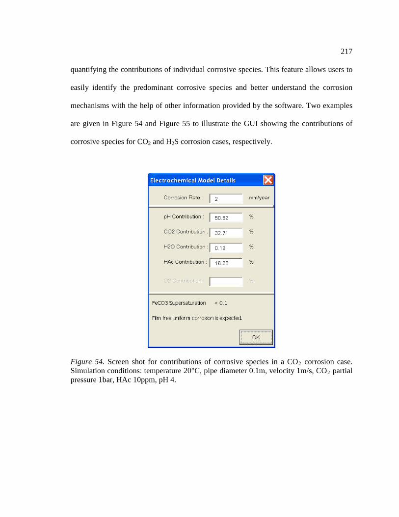
217 quantifying the contributions of individual corrosive species. This feature allows users to
easily identify the predominant corrosive species and better understand the corrosion
mechanisms with the help of other information provided by the software. Two examples
are given in Figure 54 and Figure 55 to illustrate the GUI showing the contributions of
corrosive species for CO2 and H2S corrosion cases, respectively.
Figure 54. Screen shot for contributions of corrosive species in a CO2 corrosion case. Simulation conditions: temperature 20°C, pipe diameter 0.1m, velocity 1m/s, CO2
partial pressure 1bar, HAc 10ppm, pH 4.

218
Figure 55. Screen shot for contributions of corrosive species in a H2S corrosion case. Simulation conditions: temperature 20°C, pipe diameter 0.1m, velocity 1m/s, CO2 partial pressure 1bar, H2
S 10ppm, pH 4.
Corrosion mechanisms can be further investigated by visualizing the diagram
associated with the dominant corrosion process. For CO2/HAc corrosion, which is
electrochemical in nature, polarization (E-i) curves are shown for each individual
electrochemical reaction and total anodic and cathodic reactions. The potentiodynamic
sweep curve is also shown on the same diagram. Each of the polarization curves can be
freely turned on/off for enhanced visibility and customized presentation of the corrosion
process. For H2S corrosion, where mass transfer is a concern, FREECORP gives the
concentration profile of H2S across the mass transfer boundary layers, including inner
makinawite film, outer porous makinawite layer and liquid phase diffusion boundary
layer. Figure 56 and

219 Figure 57 demonstrate two examples of the main software interface in which an Evans
diagram and an H2S concentration profile are shown for CO2 and H2S corrosion,
respectively.
Figure 56. Screen shot for the user input/output window for CO2
corrosion in FREECORP.

220
Figure 57. Screen shot for the user input/output window for H2
S corrosion in FREECORP.
Another unique feature of the model is that any electrochemical reactions,
including built-in reactions and user-defined reactions, can be added to or removed from
the corrosion process. With this feature, the effect of each reaction can be clearly
identified through the variation of corrosion rate resulting from the addition or removal of
a particular reaction. By accommodating user-defined reactions, the applicability of the
model is expanded to other steel/environmental systems where electrochemical reaction
kinetics are available. The user-defined reaction participates in the calculation process by
including a text file containing all necessary parameters in the folder where the program
is located. A certain format is required for the text file. Figure 58 shows a template of the
text file, which contains required parameter values in an acceptable format.
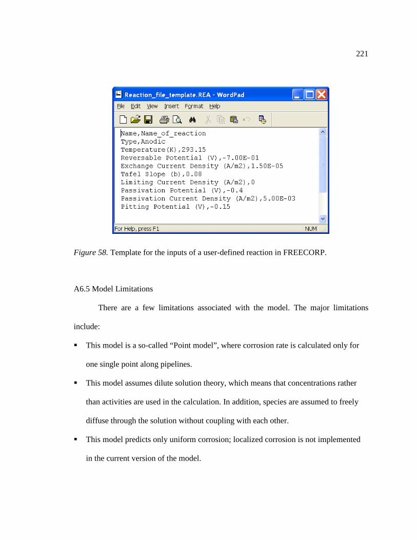
221
Figure 58. Template for the inputs of a user-defined reaction in FREECORP.
A6.5 Model Limitations
There are a few limitations associated with the model. The major limitations
include:
This model is a so-called “Point model”, where corrosion rate is calculated only for
one single point along pipelines.
This model assumes dilute solution theory, which means that concentrations rather
than activities are used in the calculation. In addition, species are assumed to freely
diffuse through the solution without coupling with each other.
This model predicts only uniform corrosion; localized corrosion is not implemented
in the current version of the model.
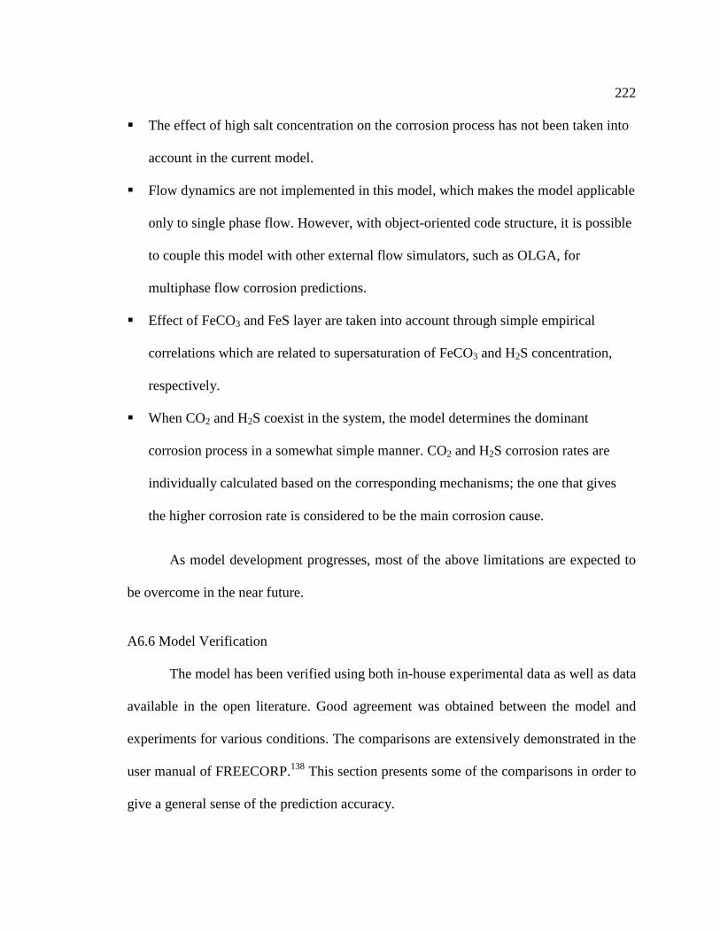
222 The effect of high salt concentration on the corrosion process has not been taken into
account in the current model.
Flow dynamics are not implemented in this model, which makes the model applicable
only to single phase flow. However, with object-oriented code structure, it is possible
to couple this model with other external flow simulators, such as OLGA, for
multiphase flow corrosion predictions.
Effect of FeCO3 and FeS layer are taken into account through simple empirical
correlations which are related to supersaturation of FeCO3 and H2S concentration,
respectively.
When CO2 and H2S coexist in the system, the model determines the dominant
corrosion process in a somewhat simple manner. CO2 and H2S corrosion rates are
individually calculated based on the corresponding mechanisms; the one that gives
the higher corrosion rate is considered to be the main corrosion cause.
As model development progresses, most of the above limitations are expected to
be overcome in the near future.
A6.6 Model Verification
The model has been verified using both in-house experimental data as well as data
available in the open literature. Good agreement was obtained between the model and
experiments for various conditions. The comparisons are extensively demonstrated in the
user manual of FREECORP.138 This section presents some of the comparisons in order to
give a general sense of the prediction accuracy.
223
Figure 59 shows the comparison between predicted and measured polarization
curves. Although no direct comparison can be made for individual electrochemical
reaction kinetics, good agreement is obtained between measured and predicted
potentiodynamic sweeps. The total cathodic and anodic polarization curves indicate that
corrosion is under charge transfer control at the corrosion potential under tested
conditions. Therefore, it can be expected that corrosion rate would not change with
further increase of velocity. This case clearly demonstrates the value of the model in
elucidating the corrosion mechanisms, which is not easily achieved through experiments.
-1
-0.9
-0.8
-0.7
-0.6
-0.5
-0.4
-0.3
-0.2
-0.1
0
0.1 1 10i / (A/m2)
E v
s. S
HE
/ V
H+ reductionH2CO3 reduction
total cathodic
total anodic(Fe dissolution)
H2O reduction
model sweep
experimental sweep
i corr
E corr
Figure 59. Comparison of experimental and FREECORP predicted polarization curves for temperature 20°C , partial pressure of CO2 1bar, solution pH 4 and velocity 2 m/s.16
Figure 60 shows the comparisons between the model and experiments for varied
CO2 partial pressure and velocity. Good agreement is achieved under all conditions. The

224 figure indicates that measured corrosion rates hardly change with increasing velocity
under relatively high CO2 pressure. This is because, under the tested conditions,
corrosion process is largely limited by the CO2 hydration rate, which is not sensitive to
the change in flow. It can be seen that this behavior is successfully captured by the
model; no significant corrosion rate change is predicted with change in velocity.

225
Figure 60. Comparison between FREECORP predictions and experiments for different partial pressure of CO2. Test condition: temperature 60°C, pH 5, pipe diameter 0.1 m. Data is taken from ICMT database.16
Figure 61 shows the predicted and measured corrosion rate as a function of HAc
concentration. Both the model and the experiments suggest an increase in corrosion rate
with increasing HAc concentration. Compared to Figure 60, it is evident that the
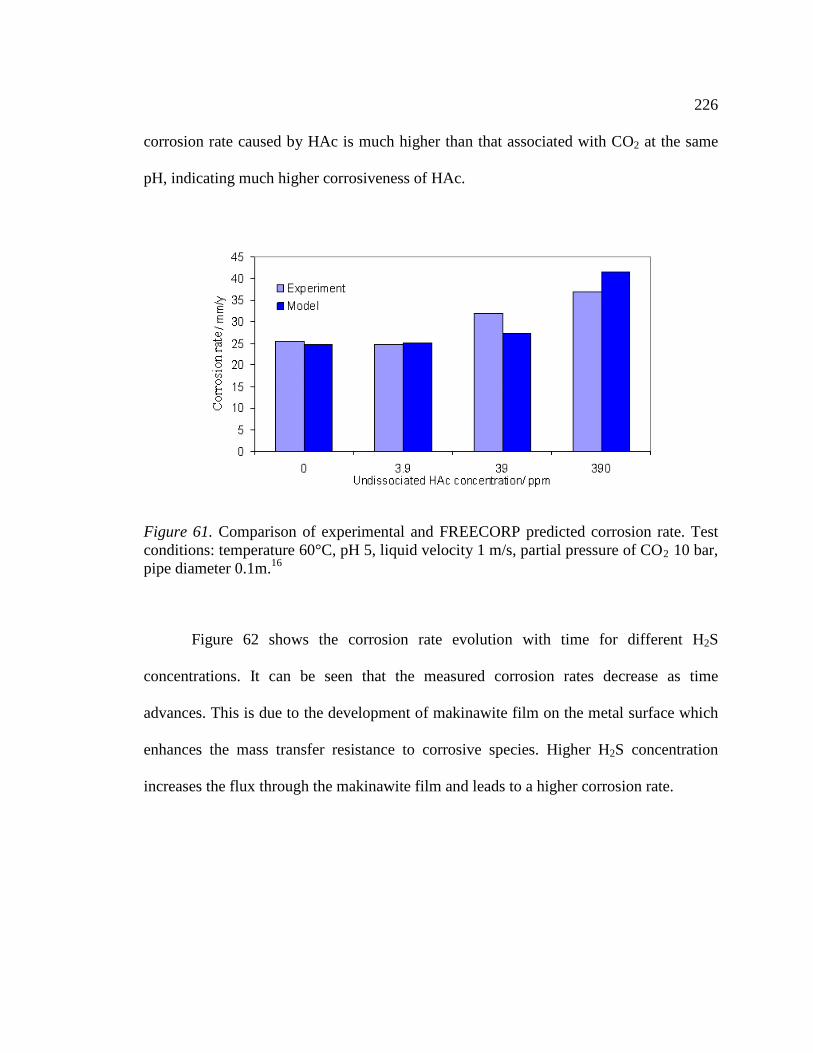
226 corrosion rate caused by HAc is much higher than that associated with CO2 at the same
pH, indicating much higher corrosiveness of HAc.
Figure 61. Comparison of experimental and FREECORP predicted corrosion rate. Test conditions: temperature 60°C, pH 5, liquid velocity 1 m/s, partial pressure of CO2 10 bar, pipe diameter 0.1m.16
Figure 62 shows the corrosion rate evolution with time for different H2S
concentrations. It can be seen that the measured corrosion rates decrease as time
advances. This is due to the development of makinawite film on the metal surface which
enhances the mass transfer resistance to corrosive species. Higher H2S concentration
increases the flux through the makinawite film and leads to a higher corrosion rate.
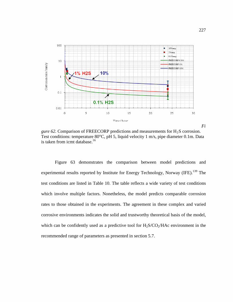
227
Figure 62. Comparison of FREECORP predictions and measurements for H2S corrosion. Test conditions: temperature 80°C, pH 5, liquid velocity 1 m/s, pipe diameter 0.1m. Data is taken from icmt database.16
Figure 63 demonstrates the comparison between model predictions and
experimental results reported by Institute for Energy Technology, Norway (IFE).139 The
test conditions are listed in Table 10. The table reflects a wide variety of test conditions
which involve multiple factors. Nonetheless, the model predicts comparable corrosion
rates to those obtained in the experiments. The agreement in these complex and varied
corrosive environments indicates the solid and trustworthy theoretical basis of the model,
which can be confidently used as a predictive tool for H2S/CO2/HAc environment in the
recommended range of parameters as presented in section 5.7.

228
Figure 63. Comparison of measured and FREECORP predicted corrosion rates under the conditions listed in Table 10.16
Table 10. Test conditions taken from open literature139 for FREECORP verification Parameters Case 1 Case 2 Case 3
Temperature, °C 80 25 80
pCO2, bar 3.3 3.3 10.0
pH2S, bar 10 10 30
Solution pH 3.10 3.20 2.90
Pipe diameter, m 0.015 0.015 0.015
Velocity, m/s 1 1 1
Duration, days 19 21 15

229 A6.7 Conclusions
A mechanistic model is developed in this work to predict uniform corrosion of
carbon steel in CO2, H2S, HAc and/or O2 environment. The model, called FREECORP, is
built based exclusively on open literature and is freely available to public users. The
model is written as a Microsoft Excel® add-in, the source code of which is made open to
the public. An object orient programming approach was adopted in developing the source
code, which allows for easy modification of the model. FREECORP provides the
flexibility of adding or removing any built-in reactions as well as user-defined reactions
into or from the system. This provides a tool to evaluate the effect of individual reactions
on the overall corrosion process. Apart from corrosion rate, the model provides other
valuable information to assist with the understanding of underlying corrosion
mechanisms. Contribution of individual corrosive species to overall corrosion rate can be
quantified for easy identification of the main corrosive species. For CO2/ HAc / O2
corrosion with electrochemical process dominant, polarization curves are given for
individual reactions as well as total anodic and cathodic reactions. For H2S corrosion,
where mass transfer limiting is assumed, the concentration profile of H2S across the inner
and outer makinawite films and the liquid boundary layer are displayed.
The model has been extensively verified against a large number of experiments,
taken both from in-house databases and the open literature. Good agreement is achieved
under various conditions, reflecting a solid theoretical root in the model. The model can
confidently be used in the parameter range within which verification was performed. The
recommended range of parameters are: temperature 20 to 120ºC; pipe diameter 0.01 to 1

230 m; liquid velocity 0.001 to 20 m/s; Fe2+ 0 to 100ppm; HAc 0 to 1000ppm and pH 3 to 7.
Although the level of uncertainty might increase for the predictions made beyond this
range, it should still be able to provide good guidance as to the corrosivity of the
environment, owing to the mechanistic nature of the model.