a method for estimating gas hydrate and free gas ...abstract. i propose a method for estimating gas...

Abstract. I propose a method for estimating gas hydrate and free gas concentrationsversus depth in marine sediments, using Gassmann's equation. The theory modelsgas hydrate- and free gas-bearing sediments partially saturated with water. A quali-tative estimate of the concentrations can be obtained by comparing the theoreticalvelocity for full-water saturation to the experimental velocity, evaluated by a tomo-graphic analysis or available from well logging. Positive anomalies indicate the pre-sence of gas hydrate and negative anomalies indicate the presence of free gas. Aquantitative estimate of concentrations is obtained by fitting the theoretical velocityto the experimental velocity. The method has been tested against sonic log and VSPdata and indirect estimations of gas hydrate concentration from chloride content incore logs.

1. Introduction

Gas hydrates (a type of chlatrates) area solid phase composed of water and low-molecular-weight gases (predominantly methane) which form under low temperature, high pressure, andadequate gas concentrations. These conditions are common in the upper few hundred meters ofrapidly accumulated marine sediments (Claypool and Kaplan, 1974).

The presence of gas hydrates in marine sediments is generally related to the so-called BottomSimulating Reflectors (BSR), a seismic event that mimics the relief of the sea floor. These reflec-tions mark the pressure- and temperature-dependent base of the methane-hydrate stability field(e.g., Shipley et al., 1979). BSR's have high-amplitudes, and are associated with a phase reversal(Shipley et al., 1979), caused by the strong acoustic impedence contrast between the hydrate-bea-

VOL. 40, N. 1, pp. 19-30; MARCH 1999BOLLETTINO DI GEOFISICA TEORICA ED APPLICATA

Corresponding author: U. Tinivella; Osservatorio Geofisico Sperimentale, P.O. Box 2011 Opicina, 34016Trieste, Italy; tel: +39 040 2140341; fax: +39 040 327307; e-mail: [email protected]

© 1998 Osservatorio Geofisico Sperimentale

A method for estimating gas hydrate and freegas concentrations in marine sediments

U. TINIVELLA

Osservatorio Geofisico Sperimentale, Trieste, Italy

(Received January 14, 1999; accepted April 30, 1999)

19

20

Boll. Geof. Teor. Appl., 40, 19-30 TINIVELLA

ring sediments and the underlying free gas layer.The elastic properties of ice are similar to those of hydrate, so the properties of permafrost

are often compared with those of hydrated sediments (Sloan, 1990). Timur (1968) proposed athree-phase time-average equation based on slowness averaging (Wyllie's equation) for model-ling consolidated permafrost sediments. The problem of transition from “suspension to compac-ted” sediment was treated with combined models. For instance, averaging bulk moduli weightedwith the respective porosities (Voigt's model; Voigt, 1928) gives a simple model for consolidatedsediments, while averaging the reciprocal of bulk moduli (Reuss's model; Reuss, 1929) accountsfor unconsolidated media. Zimmerman and King (1986) used the two-phase theory developed byKuster and Toksöz (1974), assuming that unconsolidated permafrost can be approximated by anassemblage of spherical quartz grains imbedded in a matrix composed of spherical inclusions ofwater and ice. Minshull et al. (1994) obtain an effective medium 1 by time averaging the solidand gas hydrate phases; then a medium 2 for water-filled sediment from Gassmann's equation,and finally, they time average media 1 and 2 to obtain the velocity of the partially saturated sedi-ment. Lee et al. (1996) propose that the interval velocity for hydrated deep marine sediment canbe estimated from a weighted mean of the three-phase time average equation and the three-phaseWood equation (Wood, 1941). Recently, two mechanical schemes of hydrated deposition in thepore space were proposed (Ecker et al., 1998). In the first scheme, the hydrate may cement graincontacts, which are the weakest structural components of the granular frame. In the second case,the gas hydrate is deposited away from the grain contacts; so, it only weakly affects the stiffnessof the granular frame.

In this paper, I use Domenico's approach (Domenico, 1977) to model the acoustic propertiesof the different layers related to the BSR. The aim is to quantify the concentrations of gas hydra-te and free gas in the pore space.

The concentrations can be estimated by fitting theoretical velocity to the experimental velo-city, obtained from traveltime inversion or from sonic logs. Positive anomalies indicate the pre-sence of gas hydrate and negative anomalies the presence of free gas. In the following, themethod is tested against sonic log and VSP data and indirect estimations of gas hydrate concen-tration from chloride content in core logs (Paull et al., 1996).

2. The velocity model

The compressional and shear wave velocities can be expressed as

VC

k k

C C

k

pm

eff m

f

eff

eff b eff fm

eff f

m

= +⎛⎝⎜

⎞⎠⎟

++ − − ⋅⎛

⎝⎜⎞⎠⎟

⋅ −( )

− − +

⎡

⎣

⎢⎢⎢⎢

⎤

⎦

⎥⎥⎥⎥

⋅−

⎛⎝⎜

⎞⎠⎟

⎧

⎨⎪⎪

⎩⎪⎪

⎫

⎬⎪⎪

⎭⎪⎪

1 43

1 2 1

11

1

1 2

μ

φ ρρ

βφ

β

φ β φρ

φ ρρ

( ),

/

(1)

and

respectively (Domenico, 1977). The symbols are explained in Appendix 1.I apply these equations to three different situations:

1. full water saturation; 2. water and gas hydrates in the pore space; 3. water and gas in the pore space.

I assume that the composite fluid and solid compressibilities lie between the Voigt and Reussaverages (Schön, 1996). They are given by

respectively.The pore compressibility Cp can be derived from a pore volume empirical function

(Domenico, 1977) or, alternatively, from the definition of the compressibility (e.g.,Handbook ofChemistry and Physics, 1992).

To take into account the effects due to the cementation of the grains at high concentrationsof gas hydrate, I use a percolation model (Leclaire, 1992). The percolation theory describes thetransition of a system from the continuous state (grains completely cemented) to the disconti-nuous state (uncemented grains). During this process, connections appear or disappear amongthe elements of the system. The induced modifications of the system configuration are governedby a general power law, in such way that shear modulus of the matrix takes the form

where μsmKT is Kuster and Toksöz's shear modulus (Kuster and Toksöz, 1974) and μsm0 is theshear modulus without cementation (no gas hydrate). This equation models the increasing stiff-ness of marine sediments with the increasing gas hydrate concentration (Carcione and Tinivella,1999).

Finally, the coupling factor k describes the degree of coupling between pore fluid andframe. It ranges from one (no coupling) to infinity (perfect coupling) and is related to the fre-quency of elastic waves. Note that when the coupling factor between the pore fluid and thesolid matrix is perfect (zero-frequency case), the velocities are independent of frequency

μ μ μ φ φ μsm smKT sm h s sm= −[ ] −( )[ ] +0

3 8

01/.

C s C s Cs

C

s

Cb s s h hs

s

h

h

= ⋅ ⋅ + ⋅( ) + ⋅ +⎛⎝⎜

⎞⎠⎟

−12

12

1

,

C s C s Cs

C

s

Cf w w g gw

w

g

g

= ⋅ ⋅ + ⋅( ) + ⋅ +⎛

⎝⎜⎞

⎠⎟

−12

12

1

,

V

k

s

meff f

m

=−

⎛⎝⎜

⎞⎠⎟

⎡

⎣

⎢⎢⎢⎢⎢

⎤

⎦

⎥⎥⎥⎥⎥

μ

ρφ ρ

ρ1

1 2/

21

Boll. Geof. Teor. Appl., 40, 19-30Estimation of gas hydrate and free gas

(2)

(3)

(4)

(5)

(Domenico, 1977).

3. Examples

In order to use equations 1 and 2 for evaluating gas hydrate and free gas concentrations, it isnecessary to know the variations of the material properties versus depth. I assume that the com-pressibilities and densities of the solid components are constant.

Figure 1 shows the calculated compressional and shear velocities for gas-hydrate and free-

22


Fig. 1 - Top: Calculated compressional wave velocity for gas hydrate-bearing (a) and free gas-bearing (b) sedimentsversus depth and clathrate and free gas concentrations. Bottom: Calculated shear wave velocity for gas hydrate-bea-ring (c) and free gas-bearing (d) sediments versus depth and gas hydrate and free gas concentrations.

gas-bearing sediments versus depth and gas hydrate and free gas concentrations. The values ofthe parameters for normally compacted terrigenous sediments are given in Appendix B. I assu-med that height of the water column is h=2 km and k=∞.

When the hydrate and free gas concentrations are zero, the velocity is that of the water-filledsediment. As expected, both velocities Vp and Vs increase as the gas hydrate concentration increases,particularly for large amounts of gas hydrate. On the other hand, the compressional velocity increa-ses for high free gas concentration, since the density decreases faster than the compressibility.

4. Lee et al.'s model for hydrated sediments

Lee et al. (Lee et al., 1996) proposed that the interval velocity for hydrated deep marine sedi-ment can be estimated from a weighted mean of the Pearson et al. (1983) three-phase time ave-rage equation and the three-phase Wood equations (Wood, 1941), following the approach ofNobes et al. (1986). This weighted mean of equations can be written as

Vp1 is the compressional velocity by the Wood equation given by

where Vw is the compressional velocity of water, Vh is the compressional velocity of pure hydra-te, and Vsm is the compressional velocity of the matrix. Vp2 is the compressional velocity by thetime-average equation

W is a weighting factor and n is a constant simulating the rate of lithification with hydrate con-centration.

The weight W is only a function of velocity and porosity, but it has an implicit relationshipwith depth, because the porosities and velocities of sediments depend on depth. For the parame-ter n, when the hydrates are disseminated throughout the pore space, the lower n such as n=1 maybe better suited for the velocity computation. On the other hand, if the hydrates are layered or,selectively cement grains, then a larger n may be applicable.

1

2V V V Vp

w

w

h

h

s

sm

= + +φ φ φ.

1

12 2 2 2ρ

φρ

φρ

φρm p

w

w w

h

h h

s

s smV V V V= + +

1 1 1 1

1 2V

W c

V

W c

Vp

hn

p

hn

p

=−( ) +

− −( )φ φ.

23


(6)

(7)

(8)

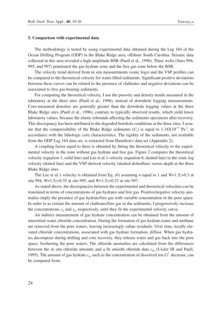
5. Comparison with experimental data

The methodology is tested by using experimental data obtained during the Leg 164 of theOcean Drilling Program (ODP) in the Blake Ridge area, offshore South Carolina. Seismic datacollected in this area revealed a high amplitude BSR (Paull et al., 1996). Three wells (Sites 994,995, and 997) penetrated the gas hydrate zone and the free gas zone below the BSR.

The velocity trend derived from in situ measurements (sonic logs) and the VSP profiles canbe compared to the theoretical velocity for water-filled sediments. Significant positive deviationsbetween these curves can be related to the presence of clathrates and negative deviations can beassociated to free gas-bearing sediments.

For computing the theoretical velocity, I use the porosity and density trends measured in thelaboratory at the three sites (Paull et al., 1996), instead of downhole logging measurements.Core-measured densities are generally greater than the downhole logging values at the threeBlake Ridge sites (Paull et al., 1996), contrary to typically observed results, which yield lowerlaboratory values, because the elastic rebounds affecting the sediments specimens after recovery.This discrepancy has been attributed to the degraded borehole conditions at the three sites. I assu-me that the compressibility of the Blake Ridge sediments (Cs) is equal to 1.34X10-11 Pa-1, inaccordance with the lithologic core characteristics. The rigidity of the sediments, not availablefrom the ODP Leg 164 data set, is extracted from Hamilton's data set (Appendix 2).

A coupling factor equal to three is obtained by fitting the theoretical velocity to the experi-mental velocity in the zone without gas hydrate and free gas. Figure 2 compares the theoreticalvelocity (equation 1; solid line) and Lee et al.'s velocity (equation 6; dashed line) to the sonic logvelocity (dotted line) and the VSP-derived velocity (dashed-dottedline) versus depth at the threeBlake Ridge sites.

The Lee et al.'s velocity is obtained from Eq. (6) assuming n equal to 1 and W=1.5z+0.3 atsite 994, W=1.5z+0.35 at site 995, and W=1.5z+0.23 at site 997.

As stated above, the discrepancies between the experimental and theoretical velocities can betranslated in terms of concentrations of gas hydrates and free gas. Positive/negative velocity ano-malies imply the presence of gas hydrate/free gas with variable concentration in the pore space.In order to as certain the amount of clathrates/free gas in the sediments, I progressively increasethe concentrations ch and sg, respectively, until they fit the experimental velocity curve.

An indirect measurement of gas hydrate concentration can be obtained from the amount ofinterstitial-water chloride concentration. During the formation of gas hydrate,water and methaneare removed from the pore waters, leaving increasingly saline residuals. Over time, locally ele-vated chloride concentrations, associated with gas hydrate formation, diffuse. When gas hydra-tes decompose during drilling and core recovery, they release water and gas back into the porespace, freshening the pore waters. The chloride anomalies are calculated from the differencesbetween the in situ chloride amounts and a fit smooth chloride data cfit (Ussler III and Paull,1995). The amount of gas hydrate ch, such as the concentration of dissolved ion Cl

-decrease, can

be computed from:

24


25


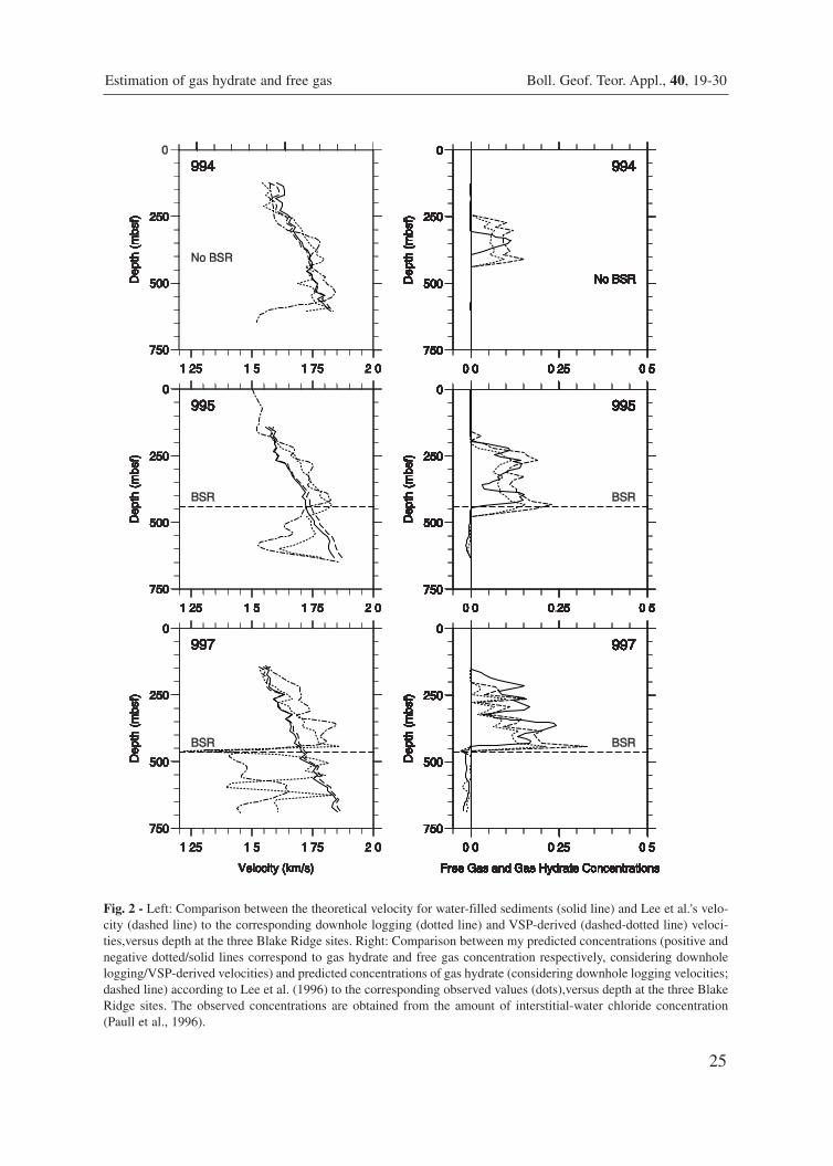
Fig. 2 - Left: Comparison between the theoretical velocity for water-filled sediments (solid line) and Lee et al.'s velo-city (dashed line) to the corresponding downhole logging (dotted line) and VSP-derived (dashed-dotted line) veloci-ties,versus depth at the three Blake Ridge sites. Right: Comparison between my predicted concentrations (positive andnegative dotted/solid lines correspond to gas hydrate and free gas concentration respectively, considering downholelogging/VSP-derived velocities) and predicted concentrations of gas hydrate (considering downhole logging velocities;dashed line) according to Lee et al. (1996) to the corresponding observed values (dots),versus depth at the three BlakeRidge sites. The observed concentrations are obtained from the amount of interstitial-water chloride concentration(Paull et al., 1996).

where cfit is the fitted chloride content, calculated in the absence of clathrates, and cCl- is the chlo-ride measurement, assuming that the chloride anomalies are solely due to gas hydrate decompo-sition during core recovery.

Figure 2 compares my theoretical concentrations (positive dotted line) and Lee et al.'s con-centrations (dashed line) of gas hydrate ch and my theoretical concentrations of free gas sg (nega-tive dotted line) estimated considering the downhole logging velocities with the correspondingexperimental curves (dots) versus depth at the three Blake Ridge sites. The solid lines in Figure2 indicate the amount of gas hydrate (positive values) and free gas (negative values) estimatedconsidering the discrepancy between the VSP-derived and the theoretical velocities evaluatedwith equation 1. No experimental profiles are available for free gas concentration. As can beseen, the prediction in my model (dotted and solid lines) is very close to the measured in situvalues. The pore-space concentration of gas hydrate estimated from the deviation of the theore-tical velocity from the VSP-derived velocity is better at sites 995 and 997, while at site 994 thedownhole logging velocity gives the most suitable estimation of gas hydrate quantities.

Quantitative differences between the theoretical and experimental concentration curves forgas hydrate depend mainly on two factors. The first is related to the rigidity and the compressi-bility in the calculation of the theoretical velocity, which are difficult to measure and which signi-ficantly influence the results. The second is related to some experimental errors in the hydrateconcentration, in the downhole logging and the VSP-derived velocities, which are fundamentalto estimate the concentrations.

Gas volume determinations (deploying Pressure Core Sampler) revealed that the pore spacecontains more than 12% of gas bubbles in the free gas zone beneath the BSR, assuming gas exi-sting in oversaturated pore water (Dickens et al., 1997). This discrepancy is probably due to amore random gas distribution in the pore space (Domenico, 1977). Moreover, the downhole log-ging and the VSP-derived velocities are not very accurate in the free gas zone due to poor boreho-le conditions.

On the other hand, the results indicate that Lee et al.'s model reproduces the correct trend,but overestimates the gas hydrate concentration. So, the accuracy of estimating the hydrate con-centration with this model is not good. The author reaches the same conclusion when applyingthe theory to permafrost (Lee et al., 1996).

6. Conclusions

I developed a simple method to estimate the concentrations of gas hydrate and free gas inmarine sediments. The model includes an explicit dependence on differential pressure and depth,and it takes into account the effects of cementation by hydrate on the shear modulus of the sedi-ment matrix. So, it is possible to model the transition between low (no cementation) and high

cc c

chfit Cl

fit

=− −

26


(9)

(cementation) gas hydrate concentration. Moreover, the theory gives both compressional andshear wave velocities, models the existence of two solids (grains and clathrates) and two fluids(water and free gas), and, finally, needs easy to hypothesize parameters.

The technique was successfully tested with a sonic log and core data available at three wellsoffshore South Carolina. When only seismic data are available, the procedure consists essential-ly in two steps. In the first step, the acoustic velocity profile is obtained from high resolution sei-smic analysis (e.g., traveltime tomography). The second step consists in estimating the concen-trations by fitting the theoretical velocities to the experimental velocities.

Acknowledgments. I thank José M. Carcione for useful discussions. I am grateful to Angelo Camerlenghi andEmanuele Lodolo for providing the preliminary experimental data. Tim Minshull, Satish C. Singh, and an anonymousreviewer provided valuable advice and thoughtful suggestions. This work was funded by the PNRA (ProgrammaNazionale di Ricerche in Antartide).

27


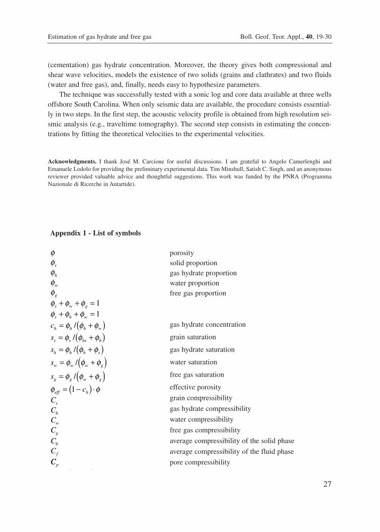
Appendix 1 - List of symbols

porositysolid proportiongas hydrate proportionwater proportionfree gas proportion

gas hydrate concentration

grain saturation

gas hydrate saturation

water saturation

free gas saturation

effective porosity

grain compressibility

gas hydrate compressibility

water compressibility

free gas compressibility

average compressibility of the solid phase

average compressibility of the fluid phase

pore compressibility

φφφφφφ φ φφ φ φ

φ φ φφ φ φφ φ φφ φ φ

φ φ φφ φ

s

h

w

g

s w g

s h w

h h h w

s s hs h

h h h s

w w w g

g g w g

eff h

s

h

w

g

b

f

c

s

s

s

s

cCCCCCC

+ + =+ + == +( )= +( )= +( )= +( )= +( )

= −( ) ⋅

11

1

/

/

/

/

/

CCp

( )

28


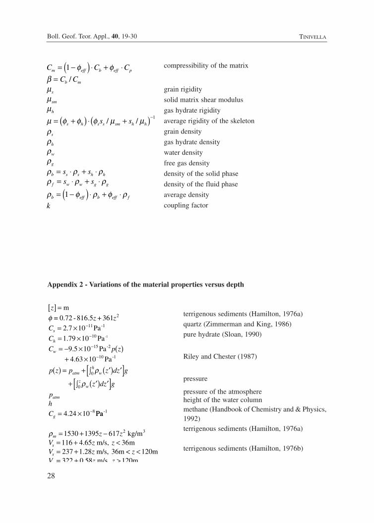
compressibility of the matrix

grain rigidity

solid matrix shear modulus

gas hydrate rigidity

average rigidity of the skeleton

grain density

gas hydrate density

water density

free gas density

density of the solid phase

density of the fluid phase

average density

coupling factor

C C C

C C

s s

s ss s

k

m eff b eff p

b m

s

sm

h

s h s s sm h h

s

h

w

g

b s s h h

f w w g g

b eff b eff f

= −( ) ⋅ + ⋅=

= +( ) ⋅ +( )

= ⋅ + ⋅= ⋅ + ⋅

= −( ) ⋅ + ⋅

−

1

1

1

φ φβμμμμ φ φ φ μ μρρρρρ ρ ρρ ρ ρρ φ ρ φ ρ

/

/ /

Appendix 2 - Variations of the material properties versus depth

terrigenous sediments (Hamilton, 1976a)

quartz (Zimmerman and King, 1986)

pure hydrate (Sloan, 1990)

Riley and Chester (1987)

pressure

pressure of the atmosphereheight of the water columnmethane (Handbook of Chemistry and & Physics,1992)terrigenous sediments (Hamilton, 1976a)

terrigenous sediments (Hamilton, 1976b)

z

z z

C

C

C p z

p z p z dz g

z dz g

ph

C

s

h

w

atm wh

wz

atm

g

[ ] =

= ×= ×= − × ( )

+ ×( ) = + ′( ) ′∫[ ]

+ ′( ) ′∫[ ]

= ×

−

−

−

−

−

m

= . - . +2.7 10 Pa

1.79 10 Pa

9.5 10 Pa

4.63 10 Pa

4.24 10

11 -1

10

15 -2

10 -1

8

-1

φ

ρ

ρ

0 72 816 5 361 2

0

0

PaPa

kg/m116 4.65 m/s, 3 m2 1.28 m/s, 36m < 120m322 58 m/s 120m

-1

3ρm

s

s

z zV z zV z zV z z

= + −= + <= + <= + >

1530 1395 6176

370

2

29


References

Carcione J. M. and Tinivella U.; 1999: Bottom simulating reflectors: seismic velocities and AVO effects. Geophysics, inpress.

Claypool G. E. and Kaplan I. R.; 1974: Methane in marine sediments. In: Kaplan, I. R. (ed), Natural Gases in marinesediments, pp. 99-139.

Dickens G. R., Paull C. K., Wallace P. and the ODP Leg 164 Scientific Party; 1997: Direct measurements of in situmethane quantities in a large gas-hydrate reservoir. Nature, 385, 426-428.

Domenico S. N.; 1977: Elastic properties of unconsolidated porous sand reservoirs. Geophysics, 42, 1339-1368.

Ecker C., Dvorkin J. and Nur A.; 1998: Structure of hydrated sediments from seismic and rock physics. Geophysics, 63,1659-1669.

Fofonoff N. P. and Millard R. C. Jr.; 1983: UNESCO Technical Papers in Marine science. 44, 1983.

Hamilton E. L.; 1976a: Variations of density and porosity with depth in deep-sea sediments. Journal of SedimentaryPetrology, 46, 280-300.

Hamilton E. L.; 1976b: Shear-wave velocity versus depth in marine sediments: a review. Geophysics, 41, 985-996.

Handbook of Chemistry and Physics; 1992. Chemical Rubber Co. Press, Cleveland.

Kuster G. T. and Toksöz M. N.; 1974: Velocity and attenuation of seismic waves in two-phase media: Part I. Theoreticalformulations. Geophysiscs, 39, 587-606.

Leclaire P.; 1992: Propagation acoustique dans les milieux poreux soumis au gel-Modélisation et expérience. Thèse deDoctorat en Physique, Université Paris 7, Paris.

Lee M. W., Hutchinson D. R., Collet T. S. and Dillon W. P.; 1996: Seismic velocities for hydrate-bearing sediments usingweighted equation. Journal of Geophysical Research, 101, 20347-20358.

Minshull T. A., Singh S. C. and Westbrook G. K.; 1994: Seismic velocity structure at the gas hydrate reflector, offshorewestern Colombia, from full waveform inversion. Journal of Geophysical research, 99, 4715-4734.

Nobes D. C., Villenger H., Davis F. F. and Law L. K.; 1986: Estimation of marine sediment bulk physical properties at

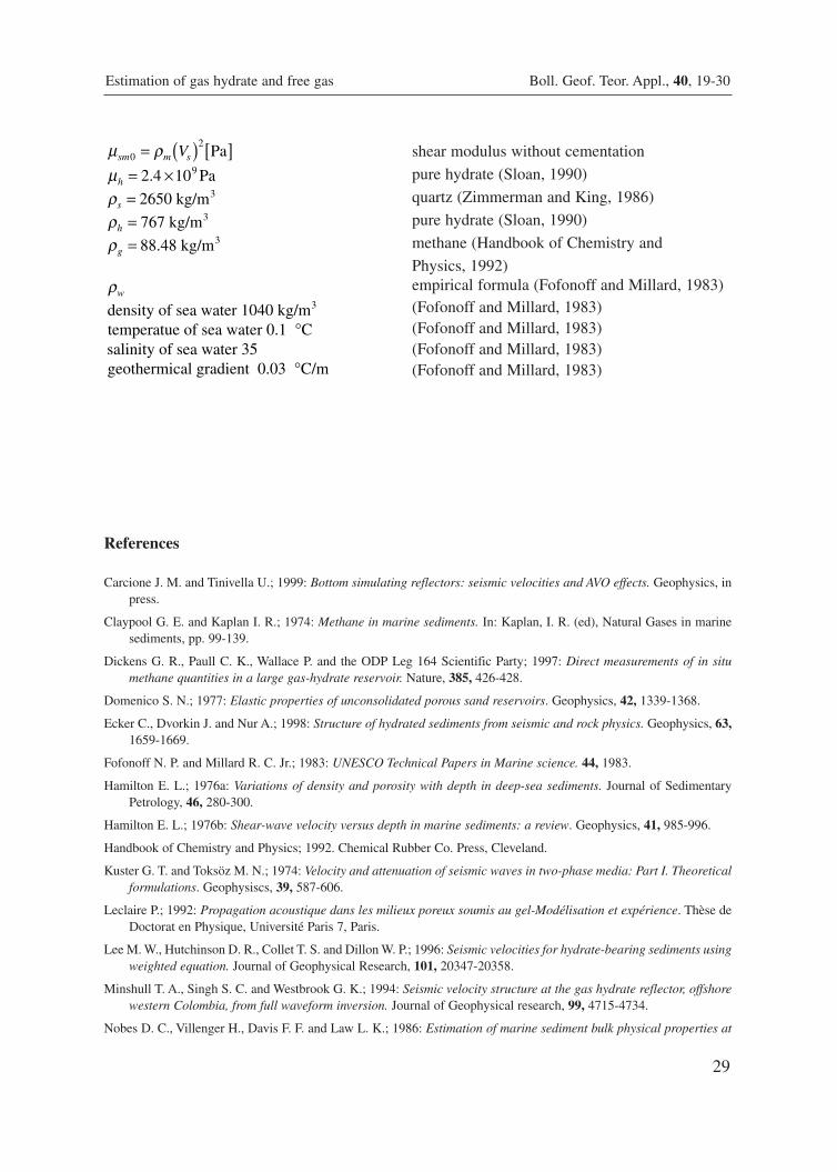
shear modulus without cementation


quartz (Zimmerman and King, 1986)


methane (Handbook of Chemistry and

Physics, 1992)empirical formula (Fofonoff and Millard, 1983)(Fofonoff and Millard, 1983)(Fofonoff and Millard, 1983)(Fofonoff and Millard, 1983)(Fofonoff and Millard, 1983)

Pa

2.4 10 Pa

2650 kg/m

767 kg/m

88.48 kg/m

density of sea water 1040 kg/mtemperatue of sea water 0.1 Csalinity of sea water 35geothermical gradient 0.03 C/m

9

3

3

3

3

μ ρμρρρ

ρ

sm m s

h

s

h

g

w

V= ( ) [ ]= ×===

°

°

02

30


depth from seafloor geophysical measurements. J. Geophys. Res., 91, 14033-14043.

Paull C. K., Matsumoto R., Wallace P. J. et al.; 1996: Proceedings of the Ocean Drilling Program. Initial Reports. TexasA&M Univ., College Station, TX, 164.

Pearson C. F., Halleck P. M., McGulre P. L., Hermes R. and Mathews M.; 1983: Natural gas hydrate; A review of in situproperties. J. Phys. Chem., 87, 4180-4185.

Reuss A.; 1929: Berechnung der Fleissgrenze von Mischkristalen auf Grund der Plastizitäts belingung für ein Kristalle,Z. Angew. Math. Mech., 9, 49-58.

Riley J. P. and Chester R.; 1987: Introduction to Marine Chemistry. Accademic Press, London, pp. 465.

Schön J. H.; 1996: Physical properties of rocks. Fundamentals and principles of petrophysics. Pergamon Press, Oxford,pp. 583.

Shypley T. H., Houston M. H., Buffler R. T. et al.; 1979: Seismic reflection evidence for widespread occurrence of pos-sible gas-hydrate horizons on continental slopes and rises. AAPG Bulletin, 63, 2204-2213.

Sloan E. D.; 1990: Clathrate hydrates of natural gas. Marcel Dekker, New York, pp.641.

Timur A.; 1968: Velocity of compressional waves in porous media at permafrost temperatures. Geophysics, 33, 584-595.

Ussler III W. and Paull C. K.; 1995: Effects of ion axclusion and isotopic fractionation on pore water geochemistryduring gas hydrate formation and decomposition. Geo-marine Letters, 15, 37-44.

Voigt W.; 1928: Lehrbuch der Kristallphysik. B. G. Terbner, Leipzig.

Wood A. B.; 1941: A text book of sound. Macmillan, New York.

Zimmerman R. W. and King M. S.; 1986: The effect of the extent of freezing on seismic velocities in unconsolidated per-mafrost. Geophysics, 51, 1285-1290.

a method for estimating gas hydrate and free gas ...abstract. i propose a method for estimating gas...

Documents