a method for robust control of systems with parametric

A Method for Robust Control of Systems

with Parametric Uncertainty Motivated by a

Benchmark Example

by

Carl S. Resnik

B.S., Aeronautics and AstronauticsMassachusetts Institute of Technology

(1986)

Submitted to the Department of Aeronautics and Astronauticsin partial fulfillment of the requirements for the degree of

Master of Science

at the

MASSACHUSETTS INSTITUTE OF TECHNOLOGY

June 1991

@ Carl S. Resnik

The author hereby grants to MIT permission to reproduce andto distribute copies of this thesis document in whole or in part.

/ 1/12 /1

Signature of Author............ . ... , --- • • -.- *-* .a......

Department of Aeronautics and AstronauticsMarc 7, 1991

Certified by ................................. , ..........Lena Valavani

Associate Professor, Department of Aeronautics and AstronauticsThesis Supervisor

A ccepted by .......................................Professortiarold Y. Wachman

oF iEmH•Y Department, Graduate Committee

J UN 1 1991LIbHARIES

A Method for Robust Control of Systems with

Parametric Uncertainty Motivated by a Benchmark

Example

by

Carl S. Resnik

Submitted to the Department of Aeronautics and Astronauticson March 27, 1991, in partial fulfillment of the

requirements for the degree ofMaster of Science

Abstract

A multivariable compensator design methodology is constructed consisting ofa model-matching, inner loop compensator and an H, outer loop compensatorto provide robust control of plants with real parametric uncertainty. The innerloop compensator desensitizes the plant to the parametric uncertainty. Theinner loop compensator is constructed by minimizing the difference between adesigner supplied desired closed loop system and the actual closed loop systemin a least squares sense. The inner loop compensator design allows for arbi-trary constraints on compensator order and structure. The H, compensatorprovides the desired closed loop performance characteristics and robustness tounstructured uncertainty. Model reduction techniques are used to reduce theorder of the H, compensator.

The methodology is applied to a (SISO) benchmark problem for robustcontrol, consisting of a mass-spring system with uncertainty in the value of thespring constant and it is shown to meet the problem stability and performancespecifications. The design approach is then applied to a multivariable mass-spring-dashpot system with simultaneous uncertainty in the spring constants.Again, robust stability and performance to parametric uncertainty is achieved.

Thesis Supervisor: Lena ValavaniTitle: Associate Professor, Department of Aeronautics and Astronautics

Acknowlegements

I would like to thank GE Aircraft Engines, especially my former boss, Mike

Idelchik, and my current boss, Sheldon Carpenter for allowing me to pursue

this degree (no matter how long it took). I would also like to thank my advisor,

Prof. Lena Valavani, for her insight and advice, which have contributed greatly

to this thesis. My coworkers lent both technical assistance and advice, while

my friends kept listening as I continually claimed to be almost done. Most of

all I'd like to thank my parents and family, especially my mother, for their

love and support in this and (almost) everything I've done.

And now, hey dudes, let's party. Hopefully my real friends will buy the

first round.

Contents

1. Introduction 19

1.1 The Problem: Parametric Uncertainty and Robust Control . 19

1.2 M otivation . . . . .. . . . . .. . . . .. . . .. .. . .. . . . 21

1.3 Thesis Contribution ........................ 22

1.4 Thesis Organization ........................ 23

2. The Approach: Inner Loop and H, 24

2.1 O verview . . . . . . . . . . . . . . . . . . . . . . . . . . . ... 24

2.2 The Standard Feedback Configuration, Loopshaping, and Sta-

bility Robustness ......................... 25

2.3 Loopshaping with Both Forward and Feedback Path Compen-

sators . . . . . . . . . . . . . . . . . . . . . . . . . . . . . . . 27

2.4 Inner Loop Compensator Synthesis with a Model-Matching De-

sign M ethodology ......................... 29

2.4.1 Introduction to the Inner Loop Model-Matching Meth-

odology . . . . . . . . . . . . . . . . . . . . . . . . . . 29

2.4.2 The Model-Matching Problem . ............. 31

2.4.3 Compensator Parametrization . ............. 32

2.4.4 The Ideal Compensator . ................. 36

2.4.5 Formulating the Minimization Problem ........ . 38

2.4.6 Constraints ........................ 43

2.4.7 W eights ..... ..................... 44

2.4.8 Methodology Summary ................ . . . 44

2.5 Design of the H, Compensator .................. 46

2.6 H, Compensator Order Reduction ................ 52

2.7 Analyzing the Closed Loop System ................ .. 53

2.8 Summary of the Methodology ................ . . . 56

3. A Benchmark Problem for Robust Control Design 58

3.1 The Plant ........................ ..... 58

3.2 Design Specifications ....................... 60

3.3 Analysis of the Plant ....................... 61

3.4 Compensator Design A ...................... 62

3.4.1 Constructing the Inner Loop Compensator: Design A . 63

3.4.2 Lessons of the Inner Loop Design ............. 74

3.4.3 Constructing the H, Compensator: Design A ...... 76

3.4.4 Frequency Response of the Compensated System: De-

sign A . . . . . . . . . . . . . . . . . . . . . . . . . . . 81

3.4.5 Time Response of the Compensated System: Design A 85

3.4.6 H, Compensator Order Reduction: Design A ..... 88

3.4.7 Summary of Design A ................... 90

3.5 Compensator Design B ....................... .. 94

3.5.1 Constructing the Inner Loop Compensator: Design B . 94

3.5.2 Constructing the H,, Compensator: Design B ..... 98

3.5.3 Frequency Response of the Compensated System: De-

sign B . . . . . . . . . . . . . . . . . . . . . . . . . . . 101

3.5.4 Time Response of the Compensated System: Design B 106

3.5.5 H,~ Compensator Order Reduction: Design B ...... 107

3.5.6 Summary of Design B .................. 107

3.6 Comparison to Published Results for a Benchmark Problem for

Robust Control .......................... 111

4. A MIMO Mass-Spring-Dashpot Problem 113

4.1 Introduction ............................ 113

4.2 The Plant: A MIMO Mass-Spring-Dashpot (MSD) System . . 113

4.3 Analysis of the Plant ......................... 116

4.4 Design of the Model-Matching Inner Loop Compensator . . . 119

4.5 Design of the H, Compensator .................. 127

4.6 Analysis of the Closed Loop System ................ 129

4.7 Frequency Response of the Compensated System ....... . 133

4.8 Time Response of the Compensated System ........... 138

4.9 H, Compensator Order Reduction ................ 145

4.10 Design Summary ......................... 145

5. Conclusions and Directions for Further Research 151

5.1 Conclusions ............................ 151

5.2 Directions for Further Research .................. 154

A. Derivation of Model-Matching Design Equations 159

B. H, Compensator State-Space Realizations 162

B.1 H, Compensator State-Space Realizations for the Benchmark

Problem: Design A ........................ 163

B.1.1 State-Space Realization of the H, Compensator . ... 163

B.1.2 State-Space Realization of the Reduced Order H, Com-

pensator . . . . . . . . . . . . . . . . . . . . . . . . . . 164

B.2 Hý Compensator State-Space Realizations for the Benchmark

Problem: Design B ........................ 165

B.2.1 State-Space Realization of the H, Compensator . . . . 165


pensator . . . . . . . . . . . . . . . . . . . . . . . . . . 166

B.3 H, Compensator State-Space Realizations for the MIMO MSD

Problem . . . . . . . . . . . . . . . . . . . . . . . . . . . ... 167

B.3.1 State-Space Realization of the H, Compensator . . . . 167


pensator . .. .. . . . . . . . . . .. . . .. . . .. . 168

C. Benchmark Example: Design A Reduced Order System Time

and Frequency Response 169

D. Benchmark Example: Design B Reduced Order System Time

and Frequency Response 175

E. MIMO Example Reduced Order System Time and Frequency

Response 181

List of Figures

2.1 The Closed Loop System with Forward and Feedback Path

Compensators ........................... 25

2.2 The Standard Feedback Configuration .............. 25

2.3 The Closed Loop System, Tinner: Plant with Inner Loop Com-

pensator . . . . . . . . . . . . . . . . . . . . . . . . . . . . . . 30

2.4 Model-Matching Design Objective ................. 32

2.5 General Feedback System .................... 32

2.6 The H , Problem ......................... 47

2.7 The H, Standard Feedback Configuration with Weights . . . 48

3.1 The Mass-Spring System with Noncolocated Sensor and Actuator 59

3.2 Bode Plot of the Benchmark Problem with k = 0.5, 1.0, 2.0 . 61

3.3 The Closed Loop System with Feedforward and Feedback Path

Compensators, Showing All Inputs and Outputs ........ 62

3.4 Bode Plot of the Ideal Plant, Hd ................. 64

3.5 Bode Plot of the Ideal Compensator, Kideal . . . ........... 64

3.6 Bode Plot of the Initial Inner Loop Compensator ....... 66

3.7 Root Locus of the Closed loop System, Ti,,er, for 0.5 < k < 2.0 67

3.8 Bode Plot of the Third Order Inner Loop Compensator: Design A 68

3.9 Root Locus of the Closed loop System, Tiner, for 0.5 < k < 2.0 69

3.10 Bode Plot of The Closed Loop System, Tin,,er, for k = 0.5, 1.0, 2.0 70

3.11 Bode Plot Comparing the Desired and Actual Plants ...... 71

3.12 Bode Plot of the Model-Matching Design Inner Loop Compen-

sator . . . . . . . . . . . . . . . . . . . . . . . . . . . . . .. . 73

3.13 Root Locus of the Closed loop System, T,rinr,r for 0.5 < k < 2.0 73

3.14 Bode Plot of The Open Loop System, GKinner, for k = 0.5, 1.0, 2.0 75

3.15 Bode Plot of The Closed Loop System, Tinner, for k = 0.5, 1.0, 2.0 75

3.16 H, Design Weights and Actual Sensitivity Specification . . . 79

3.17 Bode Plot of the H, Compensator ................ 80

3.18 Root Locus of the Plant with Inner and H, Compensators for

0.5 < k < 2.0 . . . . . . . . . . . . . . . . . . . . . . . . . . . 81

3.19 Bode Plot of the Open Loop System G(Kinner + K,) for k =

0.5,1.0,2.0 ........................... 82

3.20 Bode Plot of the Closed Loop System T(s) for k = 0.5, 1.0, 2.0 83

3.21 Bode Plot of the Sensitivity Transfer Function S(s) for k =

0.5, 1.0, 2.0 . . . . . . . . . . . . . . . . . . .. . . . . . .. . 84

3.22 Bode Plot of the Transfer Function from w to z for k = 0.5, 1.0, 2.0 84

3.23 Closed Loop System Response to a Unit Impulse Disturbance 86

3.24 Bode Plot of the Transfer Function, N(s), for k = 0.5, 1.0, 2.0 87

3.25 Closed Loop System Response with Measurement Noise to a

Unit Impulse Disturbance .................... 87

3.26 Closed Loop System Response to a Sinusoidal Disturbance . . 89

3.27 Closed Loop System Response to a Unit Step in the Reference 89

3.28 Root Locus of the Design A Closed Loop System with the Re-

duced Order H, Compensator for 0.5 < k < 2.0 - Poles Near

the Origin ........................... 91

3.29 Root Locus of the Design A Closed Loop System with the Re-

duced Order H, Compensator for 0.5 < k < 2.0 ........ 91

3.30 Comparison of the Nominal System and the Limited Inner Loop

Control System to a Unit Impulse Disturbance ......... 93

3.31 Bode Plots of the Desired Plant, Hd(s), and the actual plant G(s) 95

3.32 Bode Plot of the Ideal Compensator, Kideal(s) . . . . . . . . . 96

3.33 Root Locus of the Closed Loop System, Ti,,,,,r(s) for 0.5 < k < 2.0 97

3.34 Bode Plot of the Open Loop System, GKi,,r,, ......... 99

3.35 Bode Plot of the Closed Loop System, Ti,,er. .......... 99

3.36 H. Design Weights and Actual Sensitivity Specification . . . 100

3.37 Bode Plot of the H, Compensator ................ 101

3.38 Root Locus of the Plant with Inner and H, Compensators for

0.5 < k < 2.0 . . . . . . . . . . . . . . . . . . . . . . . . . . . 102

3.39 Bode Plot of the Open Loop System G(Kin,,er + K,) for k =

0.5, 1.0, 2.0 . . . . . . . . . . . . . . . . . . . . . . . . . . . . 102

3.40 Bode Plot of the Closed Loop System T(s) for k = 0.5, 1.0, 2.0 103

3.41 Bode Plot of the Sensitivity Transfer Function S(s) for k =

0.5, 1.0, 2.0 .......................... 104

3.42 Bode Plot of the Transfer Function from w to z for k = 0.5, 1.0, 2.0105

3.43 Bode Plot of the Transfer Function, N(s), for k = 0.5, 1.0,2.0. 105

3.44 Closed Loop System Response to a Unit Impulse Disturbance 106

3.45 Closed Loop System Response to a Unit Step in the Reference 108

3.46 Closed Loop System Response with Measurement Noise to a

Unit Impulse Disturbance ..................... 108

3.47 Closed Loop System Response to a Sinusoidal Disturbance .. 109

3.48 Root Locus of the Design B Closed Loop System with the Re-

duced Order H, Compensator for 0.5 < k < 2.0 - Poles Near

the Origin ................ ............. .... 110

3.49 Root Locus of the Design B Closed Loop System with the Re-

duced Order H. Compensator for 0.5 < k < 2.0 ........ 110

4.1 Schematic Diagram of the MIMO Mass-Spring-Dashpot Plant 114

4.2 Singular Value Plot of G for k = 0.5 ................ 117



4.5 Maximum Singular Value Plot of G for k = 0.5, 1.0, 2.0 . . . 117

4.6 Plant Pole Location for 0.5 < k < 2.0 ............... 118

4.7 Bode Plots of the Channels of the Nominal Plant ....... . 120

4.8 Bode Plots Comparing the Channels of the Desired Plant, H11 ,

to the Nominal Plant, G ..................... 121

4.9 Bode Plots of the Channels of the Ideal Compensator, Kid,,al . 122

4.10 Bode Plots of the Inner Loop Compensator, Ki,,,ner, Channels . 124

4.11 Singular Value Bode Plot of the Inner Loop Compensator, Kinne 1 24

4.12 Root Locus of the Closed Loop System, Tinner, for 0.5 < k < 2.0 125

4.13 Open Loop Singular Value Plot of GKinner for k = 0.5 . . . . 126

4.14 Open Loop Singular Value Plot of GKinn,, for k = 1.0 . . . 126

4.15 Open Loop Singular Value Plot of GKinne,. for k = 2.0 . . . . 126

4.16 Open Loop Maximum Singular Value Plot for k = 0.5, 1.0, 2.0 126

4.17 Closed Loop Singular Value Plot of Tinner for Ik = 0.5 ..... .. 128

4.18 Closed Loop Singular Value Plot of Tin,er for k = 1.0 ..... 128

4.19 Closed Loop Singular Value Plot of Tiee for k = 2.0 ...... 128

4.20 Closed Loop Maximum Singular Value Plot for k = 0.5, 1.0, 2.0 128

4.21 Bode Plots of the H, Weighting Functions, W1(s) and W.3(s),

and the Implied Constraint W((s) .............. . . . 130

4.22 Singular Value Plot of the H, Compensator .......... 130

4.23 Root Locus of the Poles of the Closed Loop System for 0.5 >

k > 2.0 . . . . . . . . . . . . . . . . . . . . . . . . . . . . . . . 131

4.24 Minimum Zeta of the Closed Loop System as a Function of k . 132

4.25 Singular Value Plot of the Open Loop Servo Transfer Function

for k = 0.5 . . . . . . . . . . . . . . . . . . . . . . . . . . . . . 134


for k = 1.0 . . . . . . . . . . . . . . . . . . . . . . . . . . . . . 134


for k = 2.0 . . . . . . . . . . . . . . . . . . . . . . . . . . . . . 134

4.28 Maximum Singular Values of the Open Loop Servo Transfer

Functions . . .. . . .. . . .. . . . . . . . . . . .. . . .. . 134

4.29 Singular Value Plot of the Open Loop Regulator Transfer Func-

tion for k = 0.5 . .. .. .. . .. .. .. .. .. ... .. .. . 135


tion for k = 1.0 . .. . . .. ... .. .. .. .. .. . .. .. . 135


tion for k = 2.0 . .. .. .. ... .. .. .. .. ... .. .. . 135

4.32 Maximum Singular Values of the Open Loop Regulator Transfer

Functions . . . . . . . . . . . . . . . . . . . . . . . . . . . . . 135

4.33 Singular Value Plot of the Closed Loop Transfer Function for

k = 0.5 . . . . . . . . . . . . . . . . . . . . . . . . . . . . . . . 136


k = 1.0 . . . . . . . . . . . . . . . . . . . . . . . . . . . . . . . 136


k = 2.0 . . . . . . . . . . . . . . . . . . . . . . . . . . . . . . . 136

4.36 Maximum Singular Values of the Closed Loop Transfer Functions136

4.37 Singular Value Plot of the Sensitivity Transfer Function for k =

0.5 . . . . . . . . . . . . . . . . . . . . . . . . . . . . . .. . . 137


1.0 . . . . . . . . . . . . . . . . . . . . . . . . . . . . . . .. . 137


2.0 .................... .............. 137

4.40 Maximum Singular Values of the Sensitivity Transfer Functions 137

4.41 Singular Values of the Transfer Function from Disturbance to

Output for k = 0.5, 1.0, 2.0 ................... 138

4.42 Singular Value Plot of the Transfer Function, N(s) for k = 0.5 139



4.45 Maximum Singular Values of the Transfer Functions, N(s) . . 139

4.46 Closed Loop System Response to an Impulse Disturbance for

k = 1.0 . . . . . . . . . . . . . . . . . . . . . . . . . . . . . . . 141


k = 1.0 . . . . . . . . . . . . . . . . . . . . . . . . . . . . . . . 141


k = 2.0 . . . . . . . . . . . . . . . . . . . . . . . . . . . . . . . 142

4.49 Closed Loop System Response to an Impulse Disturbance with

Measurement Noise for k = 0.5 ................. 142





4.52 Closed Loop System Response to a Sinusoidal Disturbance for

k = 0.5 . . . . . . . . . . . . . . . . . . . ... . . . . . . . . . . 144


k = 1.0 . . . . . . . . . . . . . . . . . . . . . . . . . . . . . . . 144


k = 2.0 . . . . . . . . . . . . . . . . . . . . . . . . . . . . . . . 146

4.55 Closed Loop System Response to a Reference Step Change for

k = 0.5 . . . . . . . . . . . . . . . . . . . . . . . . . . . . . . . 146


k = 1.0 . . . . . . . . . . . . . . . . . . . . . . . . . . . . ... 147


k = 2.0 . . . . . . . . . . . . . . . . . . . . . . . . . . . . . . . 147

4.58 Difference in the Maximum/Minimum Singular Values of the

Full and Reduced Order H, Compensators ............ 148

4.59 Root Locus of the Closed Loop System with the Reduced Order

H, Compensator for 0.5 < k < 2.0 - Poles Near the Origin . . 149

4.60 Root Locus of the Closed Loop System with the Reduced Order

H, Compensator for 0.5 < k < 2.0 ............... 149

C.1 Bode Plot of the H, Compensator ................ 170

C.2 Bode Plot of the Open Loop System G(Knn,,r + K,) for k =

0.5,1.0,2.0 . . . . . . . . . . . . . . . . . . . . . . . . . . . . . 170

C.3 Bode Plot of the Closed Loop System T(s) for k = 0.5, 1.0, 2.0 171

C.4 Bode Plot of the Sensitivity Transfer Function S(s) for k =

0.5, 1.0, 2.0 . . . . . . . . . . . . . . . . . . . . . . . . . . . . 171

C.5 Bode Plot of the Transfer Function from w to z for k = 0.5, 1.0, 2.0172

C.6 Bode Plot of the Transfer Function, N(s), for k = 0.5, 1.0, 2.0 172

C.7 Closed Loop System Response to a Unit Impulse Disturbance 173

C.8 Closed Loop System Response with Measurement Noise to a


C.9 Closed Loop System Response to a Sinusoidal Disturbance . . 174

C.10 Closed Loop System Response to a Unit Step in the Reference 174

D.1 Bode Plot of the H, Compensator ................ 176

D.2 Bode Plot of the Open Loop System G(Kinne, + K.) for k =

0.5,1.0,2.0 ........................... 176

D.3 Bode Plot of the Closed Loop System T(s) for k = 0.5, 1.0, 2.0 177

D.4 Bode Plot of the Sensitivity Transfer Function S(s) for k =

0.5, 1.0, 2.0 . . . . . . . . . . . . . . . . . . . . . . . . . . . . 177

D.5 Bode Plot of the Transfer Function from w to z for k = 0.5, 1.0, 2.0178

D.6 Bode Plot of the Transfer Function, N(s), for k = 0.5, 1.0, 2.0 178

D.7 Closed Loop System Response to a Unit Impulse Disturbance 179

D.8 Closed Loop System Response with Measurement Noise to a


D.9 Closed Loop System Response to a Sinusoidal Disturbance . . 180

D.10 Closed Loop System Response to a Unit Step in the Reference 180

E.1 Singular Value Plot of the H, Compensator .......... . 181

E.2 Singular Value Plot of the Open Loop Servo Transfer Function

for k = 0.5 .... ............. .... ..... .. ... 182


for k = 1.0 ............................. .182


for k = 2.0 ................... .......... 182

E.5 Maximum Singular Values of the Open Loop Servo Transfer

Functions .............. . .. ..... ..... .. . 182

E.6 Singular Value Plot of the Open Loop Regulator Transfer Func-

tion. for k = 0.5 ...... .... ....... ........... 183


tion for k = 1.0 ..... ..... .... ............ .. 183


tion for k = 2.0 .......................... 183

E.9 Maximum Singular Values of the Open Loop Regulator Transfer

Functions .................. ............ 183

E.10 Singular Value Plot of the Closed Loop Transfer Function for

k= 0.5 .. .......... .. ..... ...... ..... .. 184


k = 1.0 . . . . .. . .. . . . . . . . ... . . . . .. . .. . . . 184


k = 2.0 . . . . . . . . . . . . . . . . . . . . . . . . . . . . . . . 184

E.13 Maximum Singular Values of the Closed Loop Transfer Function 184

E.14 Singular Value Plot of the Sensitivity Transfer Function for k =

0.5 . . . . . . . . . . . . . . . . . . . . . . . . . . . . . . .. . 185


1.0 . . . . . . . . . . . . . . . . . . . . . . . . . . . . . .. . . 185


2.0 . . . . . . . . . . . . . . . . . . . . . . . . . . . . . . .. . 185

E.17 Maximum Singular Values of the Sensitivity Transfer Functions 185

E.18 Singular Value Plot of the Transfer Function, N(s) for k = 0.5 186



E.21 Maximum Singular Values of the Transfer Functions, N(s) . . 186

E.22 Singular Values of the Transfer Function from Disturbance to

Output for k = 0.5, 1.0, 2.0 ................... 187

E.23 Closed Loop System Response to an Impulse Disturbance for

k = 0.5 . . . . . . . . . . . . . . . . . . . . . . . . . . . . . . . 188


k = 1.0 . . . . . . . . . . . . . . . . . . . . . . . . . . . . . . . 188


k = 2.0 . . . . . . . . . . . . . . . . . . . . . . . . . . . . . . . 189

E.26 Closed Loop System Response to an Impulse Disturbance with





Measurement Noise for k = 2.0 ..... .. ... .......... 190

E.29 Closed Loop

k = 0.5 ...

E.30 Closed Loop

k = 1.0 ...

E.31 Closed Loop

k = 2.0 ...

E.32 Closed Loop

k = 0.5 ...

E.33 Closed Loop

k = 1.0 ...

E.34 Closed Loop

System Response

System Response

System Response

System Response

System Response.

System Response

System Response

System Response

to a Sinusoidal Disturbance for




to a Reference Step Change for

to a Reference Step Change for

to a Reference Step Change forto a Reference Step Change fork = 2.0 . . .

191

191

192

192

193

193

List of Tables

3.1 Poles of the Closed Loop System, Ti;nne, for k = 0.5, 1.0, 2.0 . 67

3.2 Poles of the Closed Loop System, Ti,,ne, for k = 0.5, 1.0, 2.0 . 69

3.3 Poles of the Closed Loop System, Tinner, for k = 0.5, 1.0, 2.0 . 79

3.4 Gain and Phase Margin of the Open Loop System, GK,,,,,:

Design A . . . ...... .. ...... ........ .... . 79

3.5 Gain and Phase Margin of the Open Loop System, G(Kinne +

K,): Design A .......................... 82

3.6 Closed Loop Poles of Ti,,,,,: Design B ............... 97

3.7 Gain and Phase Margin of the Open Loop System, GKinnr:

Design B . . . . . . . . . . . . . . . . . . . . . . . . . . .. .. 98

3.8 Gain and Phase Margin of the Open Loop System, G(Kinn,, +

K,): Design B ........ ........ . ......... 103

4.1 Poles of the Nominal MIMO MSD System ............ 118

4.2 Poles of the Closed Loop System, Ti,,,,, Ik = 0.5, 1.0, 2.0 . . . 125

4.3 Table of the Minimum Damping Ratio of the Closed Loop Poles 131

4.4 Multivariable Gain and Phase Margins of the Closed Loop System133

Chapter 1

Introduction

1.1 The Problem: Parametric Uncertainty

and Robust Control

This thesis deals with an important problem in multivariable control system

design, parametric uncertainty. In particular, practical methods of designing

robust compensators in the face of such uncertainty are explored. A compen-

sator design methodology is provided for systems which are modeled as finite

dimensional, linear time invariant (FDLTI) and may be realized in terms of a

set of state equations.

Uncertainty is inherent in all models of a given physical process. For FDLTI

systems it has typically been modeled as unstructured uncertainty, dynamic

structured uncertainty or real parametric uncertainty. Parametric uncertainty

is a form of structured uncertainty; it is uncertainty in the real parameters

used to construct the FDLTI model, the elements which make up the state-

space equations. For example, in a mass-spring system the value of the mass

or masses may only be known within a certain range, or some nominal value

of the mass may be known but with some uncertainty.

Consider the FDLTI system expressed as a transfer function matrix G(s).

Now G(s) may be expressed as

G(s) = C(sI - A)-'B + D

where A, B, C, D are the matrices defining the state-space equations which

describe G(s). Then G(s) or G may be written conveniently as

G = (A, B, C, D).

Given a state-space system G with real parametric uncertainty, it may be

expressed in terms of the system matrices:

G = (A+ AA, B + AB, C + AC, D + AD)

where the parametric uncertainty is represented by the perturbations AA, etc.

to the state-space matrices and the nominal system Gnom is

Gnom = (A, B, C, D).

The terms parametric uncertainty, parameter variation, etc. are used in-

terchangeably throughout this document'. Efforts to incorporate parametric

uncertainty into robustness specifications and analysis include the structured

singular value (SSV) of Doyle [11, 10], Safonov's Multivariable Stability Mar-

gin (MSM) [23], and others such as the robustness margin presented in [24] by

Sideris and Peiia. Unfortunately, the most popular of these approaches, the

SSV (gt), is conservative for multiple parameter uncertainty.

Most efforts in multi-input multi-output (MIMO) robust control of FDLTI

systems have focused on producing control methodologies which provide ro-

'These are used only in the context of FDLTI systems; time-varying parameters are nottreated here.

bust stability and nominal performance to (bounded) unstructured uncer-

tainty, such as the H 2 /H, methodologies, see for example Doyle et al [12].

Unfortunately, such methodologies are not robust for parametric uncertainty,

as shown by Craig [8]. Another alternative, the SSV based compensator de-

sign IL-synthesis technique is only approximate with no real guarantees. Some

approaches to H2 /H, which provide for real parameter variation have also

recently been developed, such as [19] by Madiwale et al. However, these tend

to yield conservative designs. The methodology introduced here does not ex-

plicitly account for parameter uncertainty but is shown to be insensitive to

it. Given a measurement of the effects of the parametric uncertainty, it could

be used to provide a non-conservative design by iterating on the inner loop

compensator design until performance or stability was bounded by the uncer-

tainty. The methodology provides the control system designer with a method

which is easily implementable, practical, and robust, and operates within the

frequency domain framework which many designers are used to working.

1.2 Motivation

The typical compensator synthesis techniques, H 2 //H, which are used to

handle bounded unstructured uncertainty are not robust to parametric un-

certainty. This stems from the fact that most compensators seek to invert

the plant, i.e. cancel the plant dynamics, and substitute desirable dynamics

specified by the designer. It is in the specifications of the desired dynamics,

by limiting the closed loop bandwidth, for example, that the unstructured un-

certainty is handled. However, parametric variation acts on the part of the

methodology involved in the plant cancellation. If the plant contains lightly

damped poles, whose locations may vary with parametric uncertainty, this may

cause the closed loop system to be unstable in the presence of that uncertainty

[8].However, since H2/H, techniques are very popular and are supported

by several computer-aided design packages, it is desirable to investigate ways

to improve their robustness to parametric uncertainty so as to be able to

routinely use them to design multivariable control systems. These techniques

also allow explicit loopshaping in the frequency domain, which is desirable from

the viewpoint of the control system designer. A method is needed, however,

which will desensitize the plant inversion techniques of H 2/H, to parametric

uncertainty. In [8] the use of (full-state) inner feedback loops was shown

to accomplish this goal. Unfortunately, most control designs do not have

the benefit of full-state feedback, so a method of output feedback dynamic

compensation was needed to provide the same benefit. Such a method is

developed here based on a model-matching feedback path compensator which

is wrapped around the plant before an H, compensator is constructed.

1.3 Thesis Contribution

This thesis contributes a design methodology for the synthesis of MIMO com-

pensators which produce a closed loop system robust to bounded parametric

and unstructured uncertainty. The approach used is the construction of an

inner loop, feedback path, model-matching compensator which is insensitive

to parametric uncertainty, and a unity feedback, forward path compensator

which is insensitive to unstructured uncertainty and provides closed loop per-

formance, disturbance rejection, command following, etc.

The approach presented does not explicitly account for parameter variation.

The inner loop compensator is insensitive to parametric variation because it

is a feedback compensator designed without attempting to cancel the plant

dynamics. Other advantages of the inner loop design methodology allow for the

designer to set the compensator order and impose arbitrary constraints on the

compensator structure. Inner loop performance is specified in the frequency

domain. The outer loop is constructed using the HE, methodology which also

allows for explicit frequency domain performance specifications and robustness

to unstructured uncertainty.

It is the intention that this methodology be a systematic, easy to use

approach to constructing compensators for problems with parametric uncer-

tainty.

1.4 Thesis Organization

The thesis is organized into five chapters.

The first chapter has been the introduction. In Chapter 2 a comprehensive

explanation of the compensator methodology, used to robustify the sys-

tem to parametric uncertainty, is presented. Also discussed are frequency

domain loopshaping and a robustness measure.

In Chapter 3 the methodology is applied to a benchmark problem for robust

control [25]. Two separate designs are presented.

In Chapter 4 the methodology is applied to a MIMO mass-spring-damper

system.

Last, in Chapter 5, the effectiveness of the methodology is assessed and rec-

ommendations for further research are given.

Chapter 2

The Approach: Inner Loop and

Hco

2.1 Overview

This chapter presents a methodology for designing a compensator structure

which is robust in stability and performance to both the effects of parametric

uncertainty and to normal additive or multiplicative unstructured uncertainty.

The methodology involves first construction of an inner loop, feedback path,

compensator using a model-matching design technique. This compensator re-

duces the effects of parametric uncertainty on the system. An H, outer loop

compensator is then designed to provide robust system performance. The

reason for choosing this approach stems from needing to desensitize the H,

methodology to real parametric uncertainty since it provides a flexible, stan-

dardized architecture for designing multivariable compensators.

The methodology used here results in a closed loop system with both a

feedback path, Ki,,er, and a forward path, K,, compensator as shown in

Figure 2.1.

Figure 2.1: The Closed Loop System with Forward and Feedback Path Com-pensators

2.2 The Standard Feedback Configuration,

Loopshaping, and Stability Robustness

The H,, methodology will be used to construct compensators for use in the

standard feedback configuration. This configuration, shown in Figure 2.2, con-

sists of a plant, G, unity gain feedback of the plant outputs, y, to constructing

an error, e, by comparison with a set of reference inputs, r, and the controller,

K, operating on that error in order to provide a set of plant control inputs, u.

Figure 2.2: The Standard Feedback Configuration

For the standard feedback configuration, Figure 2.2, the common loop-

shapes which are examined are the open loop, sensitivity and complementary

sensitivity transfer functions [2, 3, 9]. For the loop broken at the plant output,

the open loop transfer function is

L,(s) = GK (2.1)

where the s subscript signifies servo. For the loop broken at the plant input,

the open loop transfer function is

L,(s) = KG (2.2)

where the r subscript signifies regulator. For SISO systems these are, of course,

equivalent. The complementary sensitivity (or closed loop) transfer function,

T(s) is expressed as

T(s) = (I + GK)-'GK. (2.3)

While the sensitivity function calculated at the plant output, S(s) is

S(s) = (I + GK)->. (2.4)

The open loop transfer functions are indicative of performance at the plant

input (regulator) versus the plant output (servo). The servo open loop transfer

function provides information on command following, disturbance rejection to

disturbances injected at the plant outputs, and insensitivity to sensor noise on

the plant outputs. The regulator open loop transfer function provides informa-

tion on disturbance rejection to disturbances injected at the plant inputs and

actuator noise insensitivity at the plant inputs. The complementary sensitivity

function provides indications of closed loop command following for a reference

input, as well as stability robustness to unstructured uncertainty, if such spec-

ifications have been developed [2, 3]. The sensitivity function provides the

transfer function from error to output or the attenuation of disturbances in-

jected at the plant output.

The sensitivity transfer function is also used to provide the MIMO gain

and phase margin of the system, [16]. This is a conservative measure of plant

stability robustness at the plant output. It can also be used to measure ro-

bustness at the plant input if the input sensitivity transfer function is used,

i.e.

Si(s) = (I + KG)- '. (2.5)

This technique is based on the multivariable Nyquist criterion and may be

computed as follows. For robustness at the plant output let a be

a = IS(s)l .. (2.6)

Then the gain/phase margins are computed as

TGM < a (2.7)

IGM > (2.8)a+1

PM = > 2 sin-' 1 ) (2.9)

where these are independent and simultaneous margins in all of the channels

of the closed loop system. The arrows indicate upward or downward gain

margin. For robustness at the plant input, Si(s) is used instead.

2.3 Loopshaping with Both Forward and

Feedback Path Compensators

For the compensator configuration used here, Figure 2.1, the equivalent for-

mulas for the transfer functions are derived as follows. The servo open loop

transfer function is obtained by breaking the loop in Figure 2.1 at the plant

output, y. The transfer function from y to y is then

L,(s) = G(K, + Kinner). (2.10)

Similarly, breaking the loop at the plant input u yields

L,(s) = (K, + Kinner)G (2.11)

the open loop regulator transfer function.

The closed loop, or complementary sensitivity, is obtained by computing

the transfer function from r to y in Figure 2.1 and is

T(s) = [I + G(K, + Kinner)]-'GK,. (2.12)

Finally, the sensitivity transfer function is computed from a fictional distur-

bance, d, which is thought to be injected at the plant output in Figure 2.1, to

y and yields

S(s) = [I + G(K, + Kin,,,e)]-. (2.13)

Notice however, that if the transfer function from the reference input r to the

tracking error e is computed from Figure 2.1, (an alternate definition of the

sensitivity) it will be

Se(s) = [I + G(Kgo + Knner)]1-(I + GKinner) (2.14)

Since specifying the tracking error specifies the command following abil-

ity of the closed loop system this means that, unlike in the standard feedback

configuration, Figure 2.2, that specifications on disturbance rejection and com-

mand following are no longer equivalent. That is now

T(s) + S(s) - 1 (2.15)

but,

T(s) + Se(s) = 1 (2.16)

which may be seen by simply adding the appropriate equations given above.

So, specifiying an S(s) does not specify a T(s).

2.4 Inner Loop Compensator Synthesis with

a Model-Matching Design Methodology

2.4.1 Introduction to the Inner Loop Model-Matching

Methodology

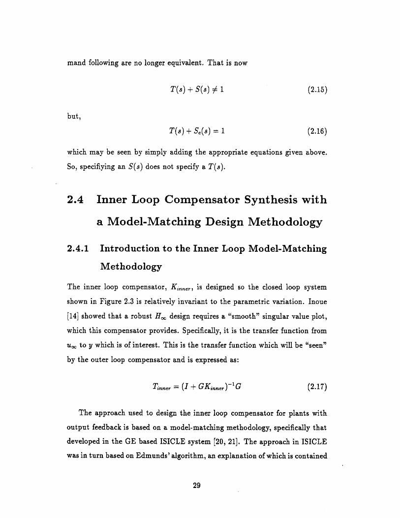
The inner loop compensator, Kinner, is designed so the closed loop system

shown in Figure 2.3 is relatively invariant to the parametric variation. Inoue

[14] showed that a robust H,_ design requires a "smooth" singular value plot,

which this compensator provides. Specifically, it is the transfer function from

u,, to y which is of interest. This is the transfer function which will be "seen"

by the outer loop compensator and is expressed as:

Tinner = (I + GKinner)-'G (2.17)

The approach used to design the inner loop compensator for plants with

output feedback is based on a model-matching methodology, specifically that

developed in the GE based ISICLE system [20, 21]. The approach in ISICLE

was in turn based on Edmunds' algorithm, an explanation of which is contained

Figure 2.3: The Closed Loop System, Tie,,r: Plant with Inner Loop Compen-sator

in [18]. The reasons for choosing this methodology are primarily its flexibility.

The methodology is amenable to dealing with square plants, i.e. those with

the same number of inputs and outputs. It allows the introduction of designer

imposed constraints on compensator structure and order. As an intermediate

step, the methodology indicates the frequency response of the compensator

needed to exactly obtain the desired closed loop performance, regardless of

whether this compensator is causal. The compensator generating algorithm

is itself iterative. Because the design method is easy to use, it allows the

designer to try several alternative designs to obtain one which best meets the

requirements.

The model-matching design methodology starts with the designer choosing

a desired closed loop transfer function Hd. For a multivariable system, the de-

signer chooses every desired closed loop transfer function element of the closed

loop transfer function matrix Hd. To do this one examines the individual nom-

inal plant transfer function matrix elements and then replaces each one with a

similar element which has the effects of the uncertainty removed. For example,

if the uncertainty is manifested in an element of the plant transfer runction

matrix as the location of lightly damped poles, one simply defines a transfer

function matrix element with those poles damped. The methodology then pro-

vides a compensator which minimizes the difference between the desired closed

loop transfer function, Hd, and the actual closed loop transfer function, H, in

a least squares sense over some specified frequency range. The minimization

process is subject to a number of designer imposed constraints. These include

selecting the compensator denominator transfer function matrix, selecting the

numerator transfer function matrix order and structure, and the frequency

range over which the minimization is to proceed. The designer can also weight

the compensator channels relative to each other.

An analysis and discussion of the methodology is provided in the following

sections. It is important to realize that this is a frequency domain methodol-

ogy, i.e. by this it is meant that it is implemented as point-by-point calculations

in the frequency domain. The importance of this will become apparent in the

realizations computed and the lack of guarantees provided by the method-

ology, though it does have a theoretical underpinnings based on the Youla

parametrization [18]. The following is based on a similar explanation for unity

feedback compensators by Minto in [20].

2.4.2 The Model-Matching Problem

The motivation for the methodology is visualized in Figure 2.4, which shows

the inner loop transfer function Tine,,, referred to here as H, in parallel with

some desired representation of the plant dynamics, Hd.

It is desired that for an input u a compensator K be constructed so the

actual output y is equal to the desired output Yd. The objective of the meth-

odology is to minimize the error, e in a least squares sense by choosing an

appropriate K, or, mathematically,

min IIHd - Hi12 (2.18)K

Figure 2.4: Model-Matching Design Objective

2.4.3 Compensator Parametrization

In this section the theoretical underpinnings which led to the use of the model-

matching algorithm are explored. It is also shown why placing the compensator

in the feedback path desensitizes the closed loop system Tinner to parametric

variation.

I/i.

Figure 2.5: General Feedback System

The Youla parametrization [13, 18] states, given the general feedback sys-

tem shown in Figure 2.5, for a stable plant G, the set of all controllers K that

stabilize G may be parameterized as

K = Q(I - GQ)-' (2.19)

where Q is any stable transfer function matrix. This result is a special case

as the Youla parametrization allows for an unstable plant G [13, 18]. The

Youla parametrization for an unstable plant could be used here, but would

only cloud the presentation. This result means that, if K stabilizes G, it must

be of the form given in equation 2.19 for some Q equal to

Q = K(I + GK)-1 . (2.20)

Also, given any stable Q, a compensator K may be obtained from equa-

tion 2.19. Notice that Figure 2.5 applies to compensators in either the forward

or feedback path.

A closed loop system H with a feedback path compensator K may be

expressed as

H = (I + GK)-1G (2.21)

from equation 2.17. Substituting equation 2.19 for K yields

H = G - GQG. (2.22)

This implies that all achievable closed loop transfer functions are also pa-

rametrized by Q. Furthermore, the desired closed loop response Hd may be

decoupled from the plant G by choosing

Q = G- 1 - G-1Hd G- 1 (2.23)

if G is square, invertible, and minimum phase. If this is substituted into

equation 2.22, it yields

H = Hd

indicating this desired transfer function is achievable. If G and Hd are square,

invertible, and minimum phase, Q is chosen as in equation 2.23, and the result

is substituted into equation 2.19, then K is shown to be

K = Hd- 1 - G- 1 (2.24)

which does not necessarily have the poles of G present in the compensator K.

This result is important in avoiding the effects of plant inversion because even

though G appears inverted in the compensator, it is present not as a product

but as a sum.

To demonstrate this consider a simple SISO example with lightly damped

poles. Let,G (s+2)(s+2)

(s + 1 + 0.1j)(s + 1 - 0.1j)

and(s+2)(s+2)S( + 1.005)(s + 1.005)

where Hd and G are identical except the lightly damped poles of G have

been moved to the real axis. Then from equation 2.24 the solution for the

compensator necessary to obtain this closed loop transfer function is

(s + 1.005)(s + 1.005) - (s + 1 + 0.1j)(s + 1 - 0.1j)(s +2)(s +2)

(s 2 + 2.01s + 1.01)- (s 2 +2s+ 1.01)(s +2)(s +2)

0.01s

(s+2)(s +2)

which has none of the poles of G present in its transfer function. Now H equals

Hd as that is the definition of equation 2.24. This provides added robustness

to the feedback path compensator for parameter variation. This can be seen

by extending the example, if there was some parameter uncertainty in G and

it actually had the transfer function

(s + 2)(s +2)(s + 2 + O.1j)(s + 2 - 0.1j)

then using equation 2.21, H would be

(s + 2)(s + 2)(s + 2)(s + 2)(s + 2)(s + 2)[.01s ± (s + 2 + 0.1j)(s + 2 - 0.1j)]

(a + 2)(s + 2)s2 + 4.01s + 4.01

(s + 2)(s + 2)(a + 2.1051)(s + 1.9049)

which shows that the actual closed loop system also has its poles on the real

axis. The lightly damped poles of G do not appear here. This example clearly

demonstrates the robustness of the feedback path compensators designed to

parameter uncertainty.

However, if a a unity feedback compensator were to be designed using the

same method, Figure 2.2, the equivalent results are as follows [20]. Since

H = (I + GK)-IGK

substituting equation 2.19 into it yields the parametrization of all closed loop

systems

H = GQ. (2.25)

Again if G is square, invertible and minimum phase then given an Hd Q may

be expressed as

Q = G- 1Hd. (2.26)

This can be substituted back into equation 2.19 to yield a compensator of the

form

K = G - 1Hd(I - Hd) - 1 . (2.27)

Notice this compensator will always have the poles of G present in it because

it is a product of the inverse of G and the desired closed loop dynamics.

2.4.4 The Ideal Compensator

As stated in equation 2.21, the transfer function H may be expressed as:

H = (I + GK)-'G.

Now, if we assume that some ideal compensator is available - even if it can't

actually be realized as G does not meet the conditions given in Section 2.4.3

- to attain the desired plant Hd, the latter may be expressed as

Hd = (I + GKideal)-1G. (2.28)

This may then be rearranged to yield

Kideal = H d-1 - G-1. (2.29)

Notice this is the form given in equation 2.24; an explicit state-space form

for Kideal is realizable only if both Hd and G are invertible. Often the ideal

compensator Kideal will not be realizable. However, the frequency response of

both G and Hd can be computed over some finite frequency vector w made up

of p discrete frequency points or

W --

W1

W 2

Wp

Then if G has m inputs and outputs, the frequency responses of G and Hd are

available as mp x m matrices expressed as

Gfr =

G(jowi)

G(jw2 )

G(jwp)

Hd(jw1)

Hdfr Hd( 2 )

Hd(jWp)

These frequency responses can then be inverted at each frequency point, wp,

to obtain Hd- and G-,1'. Therefore, Kideal may always be expressed as a

frequency response and may be thought of as the subtraction of two bode

plots or

Kideal fr = HdJ • - G .

In fact, it is not necessary to have a state-space realization of Kideal; besides

it is often not desirable as it would be of unnecessarily high order. This ideal

compensator frequency response is generally used as a guide to selecting the

order and structure of the actual compensator.

Because the ideal compensator is calculated as a frequency response, each

channel of this response can be plotted as a bode plot. Then its structure,

whether non-causal or causal, will be apparent to the designer. For example,

if rate feedback is needed to achieve the desired plant, the ideal compensator

will indicate this. Regardless of the form of the ideal compensator, information

is available to guide the designer in choosing the compensator structure or in

assessing the choice of Hd.

2.4.5 Formulating the Minimization Problem

The error in outputs between the ideal yd and the actual outptut y is defined

to be

E Hd - H. (2.30)

This may also be expressed as

E = Hd - (I+ GK)-1 G.

After some manipulation (see Appendix A) this results in

E = H(G-1Hd - I) + HKHd (2.31)

Where G- 1 is available since all of the above transfer function matrices are

given in terms of frequency responses.

Since K can be expressed as a transfer function matrix

K =_

dll d 12 dim

d21 d22

.. d . nmmd.1 dnmm

then, if the denominator transfer function matrix, Dk is fixed as

Dk =

1d1l

1

Sdidrn

1d12

d22

1dim

1dmm

equation 2.31 may be transformed into a linear least squares problem for the

numerator transfer function matrix Nk. We note Nk may be expressed as

Nk =

nil

n2l

nm1

n .12 ni

nh2 2

... nmm

The designer chooses the structure and order of Nk guaranteeing the causality

of the compensator K.

This minimization problem may then be solved on a point-by-point basis

in the frequency domain. The minimization problem shown in equation 2.31

can be more generally expressed (dropping the fr subscript)

min IrY - AKBIj 2K(2.32)

where

Y = H(G-'Hd - )

A = -H

B = DkHd

and all have been evaluated point-by-point in the frequency domain. This

problem may then be converted to the form

min HY - XEj12 (2.33)

by using the vec operator on equation 2.32 [18].

The vec operator is defined as the following. Given a matrix

Z = zI z2 z3 ]

where zlz 2, z3 are the column vectors of Z, the operation vec Z is defined as

z1

vec Z = z2

Also, given the matrices, X, YT, Z, the quantity vec (XYZ) is

vec (XYZ) = (ZT • X)vec Y

where 9 signifies a kronecker delta multiplication.

Therefore, if the frequency responses for the system are arranged as an

mm x p matrix, then for example,

yi(jiw) ... ym (jwu)y1(jW2) ... Y(jW)

L yi(jwp) ... Ym(jWp)

where each yl(jwp) is an 1 x m matrix of the form

YMUjWP) = [ ylm(ju~p) ... nmMjWP)]

Yf r

I

Notice that Nk is still in coefficient form. Therefore, for a compensator of

order 1, Nk takes the form:

1-1 • 1-1

21

-1 U -1mm

... m~(jw0)

no

·mm(jw" )

Since any element ntm may be zero, the numerators are not all constrained

to be of the same order. So applying the vec operator to equation 2.32 the

classic least squares form is obtained or

Y - XE = 0.

where

Y = vecY

X = B T 0 AE

E = vec Nk.

The matrix Y is now mml x 1 of the form

Ymrn(jwl)

ymm(jWp)

(2.34)

and the matrix BT 9 A is mm x mm. Then E results from factoring vec Nk

Nk =

nt 1ni

ni 1nm (jw)

Y

into the mm(l + 1) x 1 vector

O=

nil1

n•1-1

nmmni-1

mm

mm

made up of the constant elements of the numerator transfer function matrix

and the mm x mm(l + 1) matrix E containing the dynamics, where

0

(iW)' (jW)' 1- ... 1

) -1 ...

L0

Finally, Since it is desired that the solution

real, the problem may be restated as

to the least squares problem be

YRe XeYIm XI

(2.35)

where Y = YRý + jYIm, X = XRe + jXim. This can then be solved for a real

solution E using the numerically stable QR algorithm [18].

Therefore, returning to equation 2.31 the procedure to obtain Nk is as

follows:

1. Choose an Hd, Dk and w.

(,) (U0)-1 ...

2. Let H = Hd, E = 0.

3. Compute the appropriate frequency responses and find a least squares

solution to equation 2.31.

4. Compute H and E.

5. If e is less than some tolerance, quit, else return to step 3.

The algorithm may also be stopped after some specified number of itera-

tions. Note that the algorithm is not convex and is not guaranteed to converge.

Extensive experience shows, however, that for reasonable choices of Hd, the

algorithm will converge quickly. Generally, a few iterations will suffice. It is

recommended that the designer observe the error after each iteration and stop

the iterations when deemed appropriate.

2.4.6 Constraints

One of the advantages of this methodology is that the order of each individual

transfer function in the compensator transfer function matrix may be con-

strained. Therefore, the order of each transfer function element may be set

appropriately, usually using the ideal compensator as a guide. This is achieved

within the minimization by setting higher order terms to zero and not letting

the minimization routine act on them. Similarly, the values of any of the

individual transfer function elements and even just the individual values of a

specific numerator may be fixed and the minimization allowed to proceed. The

constraints are achieved within the minimization by moving the constrained

elements to the left side of equation 2.34.

2.4.7 Weights

Another aspect of the methodology is that it is possible to weigh individual

channels of the actual transfer function H within the minimization problem.

This may be expressed as

min I W. * (Hd - H)112 (2.36)K

Where the .* operation signifies an element-by-element multiplication. Note

that all elements of the weight matrix W must be greater than zero.

2.4.8 Methodology Summary

After several iterations of choosing ideal plants and manipulating the denom-

inators, channel weights, etc., the designer should be able to derive an inner

loop compensator which will provide the necessary damping over the full range

of parameter variation.

To summarize, the steps for constructing an inner loop compensator are as

follows.

1. A desired closed loop transfer function, Hd, in terms of channel-by-

channel desired transfer functions is obtained; Hd reflects the system

shown in Figure 2.3. The most important decisions in using the method-

ology are choosing the desired closed loop shape, Hd, the compensator

pole locations, and the numerator order. Remember the methodology

provides no guarantees, therefore it helps to choose Hd "intelligently"

with roughly the same magnitude and bandwidth of the plant. While

the methodology can provide compensators which improve the closed

loop performance, here the H, compensator will provide performance,

the inner loop is used to desensitize the plant to parameter uncertainty.

2. A frequency domain channel-by-channel representation of the ideal com-

pensator, Kideal, is obtained. It is suggested that a fairly large frequency

range be used in this step to fully obtain the ideal compensator charac-

teristics.

3. Using this ideal compensator and the constraints of the problem, the

denominators for the individual channel transfer functions are chosen

(fixing the order of the compensator). Generally, the denominators are

chosen using the ideal compensator as a guide. The shape of the ideal

compensator will also provide guidance on choosing the order of the

denominator. An advantage of this methodology is that it allows the

compensator order to be less than that of the plant. Some iteration may

be necessary to place the denominator poles correctly.

4. Any remaining constraints on the numerators are expressed; these in-

clude fixing the order of each of the elements of Nk and also constraining

any of the elements of Nk as desired, i.e. setting a particular element of

Nk to a predetermined numerator polynomial (including 0). Here one

also reflects the relative weighting of the individual channels.

5. The compensator is then optimized to reduce the least squares error be-

tween the desired plant, Hd, and the actual plant, H, point-by-point

along a given frequency vector. The frequency range chosen is a design

variable. It is recommended that the range be limited to some interval

about crossover. If the compensator or desired plant has low or high

frequency characteristics that the designer wishes to maintain, the fre-

quency range may be extended. The number of frequency points must

also be chosen so as to seek a balance between fully reflecting the plant

characteristics and achieving desirable numerical iteration speed.

6. The resulting system, Tiner, is checked to determine if it meets the

requirements.

This process is repeated as necessary until a satisfactory compensator is ob-

tained.

This methodology is useful and effective for the following reasons:

* The compensator structure chosen is inherently resistant to parametric

uncertainty, especially that affecting the plant open loop pole location.

See Section 2.4.3.

* The methodology lets the designer choose the order of the compensator

and this allows the minimization of compensator complexity (see Sec-

tion 2.4.5.

* The methdology allows the designer to work in the frequency domain,

choosing the desired closed loop system (Tinner) frequency response.

Based on this response the methodology indicates the structure of the

necessary compensator, Kinner(see Sections 2.4.2 and 2.4.4).

* The methodology is amenable to various compensator constraints (see

Section 2.4.6).

After completing the design of the inner loop compensator, one would be

ready to proceed with the outer loop design using the Ho, methodology.

2.5 Design of the Ho Compensator

The H/, methodology was chosen for the outer loop compensator because it

is a popular MIMO technique which derives closed loop system performance

through explicit frequency domain loopshaping. Ho designs tend to be robust

to unstructured uncertainty for well behaved plants. The H• design procedure

is well documented, see for example [9, 13] for the theory and [5, 8] for actual

design examples, and, therefore, it will be explained only briefly here. Though

in this application it is desired that the Ho methodology construct a compen-

sator of the standard feedback design, the methodology is very general. Given

a FDLTI system of the form shown in Figure 2.6, where

gl = exogenous inputs (references, disturbances, etc. )

u2 = control (actuator) inputs

yl = controlled outputs

Y2 = measured outputs.

The objective of the Hco methodology is: for a transfer function matrix, P'(s),

construct a stabilizing compensator, Ko(s), to minimize the closed loop trans-

fer function from ul to yl, T~1JU such that

min ITylul i o = -optim. (2.37)Kwo

Practically, one iterates on the value of 7y until it is aribrarily close to (but not

necessarily equal to) Yoptimal.

Ul

Figure 2.6: The H. Problem

.Y

The transfer function P'(s) represents the plant (in this thesis with the

inner loop compensator) augmented by some weighting functions. To solve

the problem, the H, methodology expresses this augmented plant, P' in state-

space form as

A B1 B2

P'(s) = C1 D1 D1 2

C2 D21 D22

The H, compensator is then obtained by solving two Ricatti equations, see

[12].

To design a controller for the standard feedback configuration, the H,

methodology generally uses the following approach. The plant, P (here the

original plant G with the inner loop compensator, Kinner), is augmented with

weighting functions Wl(s), W2(s), and W3 (s) as shown in Figure 2.7 to yield

an augmented plant, P'.

U1

U 2

Y13

Y12

Y11

Y2

Figure 2.7: The H., Standard Feedback Configuration with Weights

The weighting functions are used for loopshaping, where Wi(s) provides

performance and is generally the inverse of the desired sensitivity function.

W3(s) is used to provide robustness to unstructured uncertainty and is gener-

ally the inverse of the desired closed loop (complementary sensitivity) transfer

function. 4 2(s) provides any desired weighting on the controller. The trans-

fer function which is being reflected by W2 will be called R. It is the transfer

function from r to u, and is expressed as

R = K(I + GK)- 1

in terms of the standard feedback configuration as shown in Figure 2.2.

The combination of weights W1 and W3 is known as the mixed sensitivity

problem. The designer attempts to find a balance between disturbance re-

jection, as reflected by W1, and the closed loop bandwidth which will specify

robustness to unstructured uncertainty and command following performance,

reflected by W3. One of the many issues that arise in this type of problem

is whether to allow peaking in the sensitivity and complementary sensitivity

transfer functions. To allow more freedom in the design, W1 is often weighted

by a scalar p; this allows it to be adjusted independently of TW3 . If so, this sys-

tem of plant and weights may be represented as the following transfer function

matrix.

/11

Y12

Y13

Y2

pWi(s) -pWi(s)P(s)

0 W2(s)

o W3(S)P(S)

I -P(S)

Ul

U 2

The actual solution to the Ho, problem now may be expressed as

pW1 S

W 2R =7 (2.38)

W 3T

where

Y > 'Yoptimal.

The weight, W (s) used to express the constraint on the sensitivity transfer

function (the actual constraint is enforced by W 1-) is subject to a special

condition in this design. Given the system shown in Figure 2.2, the system

to which the Ho0 design process is being applied, is the standard feedback

configuration with G equal to Tinner, with the sensitivity function given as

S'(s) = (I + Tinne,Ko) - 1. (2.39)

Substituting for Tinn,r and rearranging,

S'(s) = [I + G(Kinner+ Koc)]-1(I + GKinner) (2.40)

which is equal to to S,(s) as given in equation 2.14, the transfer function from

reference r to error e. Since the sensitivity of the closed loop system with both

compensators to an output disturbance was given in equation 2.13 as

S(s) = [I + G(Koc + Kinner)]-1

this indicates that the inverse of the actual constraint placed on the sensitivity

by Wi(s) is

W(s) = (I + GKinner) W1. (2.41)

Care must be used in choosing W1 so as to restrict the disturbance sensi-

tivity function, S(s) as well as the command following properties of Se(s). If

a Wl is chosen then the weight W 1 to be used in the H, design is

W1 = (I + GKinner)'-1 W. (2.42)

Therefore, the designer can determine the desired sensitivity function relating

to an output disturbance, S(s), and check the error sensitivity function, Se(s),

or vice-versa.

Software to facilitate the standard feedback problem is commercially avail-

able as is software which solves the general H, problem, for example, the

PRO-MATLAB Robust Control Toolbox. Since the H, approach is general,

any feedback configuration, with any fictitious inputs or outputs desired, could

be used as long as the problem can be put in the form of Figure 2.6. If so it

is relatively easy to write the accompanying state-space description which will

allow this to be used with commercially available H~, software packages.

Generally, P(s) will be in state-space form while the weights are expressed

as multivariable transfer function matrices. Several methods exist to allow for

improper W3(s). W2(s) is often chosen to be of the form el, where e is some

small number, to ensure that D 12 is of full rank [5].

Explanations of how the H, methodology is applied are contained in the

design examples. For further explanation the references cited above, [5, 8] are

useful.

When the H,, design is finished, the complete compensation network will

have been designed. This compensation network should then provide stabil-

ity and performance which is robust to the range of parametric uncertainty

expected. Moreover, this design should be robust to standard design uncer-

tainties such as unmodelled dynamics, plant disturbances, etc. if a reasonable

bandwidth was selected for W3.

2.6 H, Compensator Order Reduction

One disadvantage of the H, methodology is that it leads to compensators

of high order, as an H. compensator will always have at least the order of

the augmented plant, P'(s), used to create it. High order and complexity

makes the compensator more difficult to implement. Therefore, it is desirable

to reduce the compensator order when possible. Fortunately, some amount

of compensator order reduction is usually possible. However, though the H,

methodology guarantees some amount of robust stability, all such gurantees

are lost when the compensator order is reduced. Therefore, it is very important

to check that the system with the reduced order compensator meets the same

specifications which the original system achieved.

The steps used here to reduce the order of the H, compensator are as

follows.

1. From the bode or singular value plots of the nt h order H, compensator,

estimate the number of states (k) the compensator can be reduced to.

This may be done by observing the changes in slope in the plot and

estimating the number of poles necessary to achieve those changes in

slope. The algorithms used, see (2) below, also allow the examination

of the Hankel singular values of the full order compensator which may

provide information on the number of states which can be eliminated.

2. Compute a reduced order realization of the compensator. The techniques

used herein are Schur model reduction, as implemented by the PRO-

MATLAB Robust Control Toolbox function schmr [5], and balanced

least squares model reduction, as implemented by the PRO-MATLAB

Robust Control Toolbox function balmr [5].

3. Compare the reduced order compensator to the original compensator.

This can be done in several ways. A quantitative measure of the dif-

ference in the compensators is contained in the algorithms used. Both

algorithms compute a kth order reduced compensator according to the

criterion

JJIKo - K°oloc < 2 C k-(i) (2.43)i=k+l

and return the value of 2 EZLk+l ko(i). It is also useful to compare the

Bode or singular value plots of the compensators and compute the error

as a function of frequency. If these measures are small it is likely that the

reduced order compensator will achieve the design objectives. It is ad-

visable to iterate between steps 2 and 3 until the compensator has been

reduced as much as possible while maintaining its frequency response

characteristics. The Ho methodology guarantees that the nominal sys-

tem is closed loop stable; reducing the order of the compensator removes

this guarantee. However, one is usually able to reduce the compensator

order by some amount while maintaining all of the stability and perfor-

mance results of the nominal Ho compensator.

4. Generate the compensated system with the reduced order compensator

and check the system stability, frequency response, and time domain

respoise as for the original Ho compensator. If the reduced order com-

pensator does not meet the performance of the original H. compensator,

obviously a higher order compensator should be used. If the system re-

sponse with the reduced order compensator meets the requirements, then

the design is finished.

2.7 Analyzing the Closed Loop System

This compensation network should provide stability and performance which

is robust to the range of parametric uncertainty expected. Moreover, this

design should be robust to standard design uncertainties such as unmodelled

dynamics, plant disturbances, etc. The following loopshapes will be examined

in an attempt to determine the success of a design: open loop (both servo

and regulator), closed loop, and the sensitivity. The MIMO or SISO gain

and phase margins will be calculated to determine robustness to unstructured

uncertainty.

It is also important to determine the effect of the inner loop on the plant

without the presence of the outer loop because it is unlikely that the full com-

pensation network will have desirable properties if Tinner does not desensitize

the plant to parameter uncertainty. In fact, this should be determined before

design of the outer loop begins. Therefore, one should examine the open and

closed loop shapes to determine robustness to both the parametric variation

and unstrucured uncertainty. It also important to know the characteristics of

the Tinner loop shape the H,, methodology will use.

For all of the above loop shapes the fact that this is a plant with some

amount of parametric variation must be accounted for. Therefore, it is impor-

tant to examine the loop shapes not only in terms of some nominal parameter

values for which the compensator has been designed, but also the ranges of

parameter variation to be considered. Therefore, in this thesis the following

cases are examined:

* The nominal case (also the design case).

* The minimum value of the parameter variation.

* The maximum value of the parameter variation.

The assumption of the nominal case as the design case implies that it is desired

that the system performance be optimized for this case, with the system ro-

bustness extending that performance over the range of parametric uncertainty.

The approach listed above will lead to a large number of singular value plots.

Notice that for cases of multiple parametric uncertainty one may not be

able to calculate the minimum and maximum cases of parametric variation

as these may be hard to determine. The cases examined in this thesis allow

for such a determination and were chosen as such for illustration purposes.

In a case where this information is not available, the options include use of

a multivariable margin which accounts for real parametric uncertainty, see

Section 1.1, through Monte Carlo simulation, or placing an upper (or lower)

bound on each element of the state-space matrices and assuming this reflects

the worst case.

One of the primary results of the parameter variation in the examples

considered in this thesis is that the positions of lightly damped poles will vary

with the uncertainty. Since the primary function of the inner loop will be

to damp these poles, it will also be instructive to consider the locations and

damping ratios of these poles over the range of parameter variation with the

inclusion of the inner loop compensator. This will be expressed in terms of

root locus plots and tabular listings of poles, frequencies, and damping ratios.

Time domain responses of the compensated systems are also important to

understanding the system and determining if they meet the time domain design

specifications. Several types of time response simulations will be considered.

These include:

* Injection of an impulse disturbance to determine disturbance rejection

characterisitics.

* Injection of a constant frequency sinusoidal disturbance to determine

disturbance rejection characteristics.

* Reference step commands to determine the command following charac-

teristics of the closed loop system.

* The inclusion of random Gaussian measurement noise in certain simula-

tions to determine the system noise rejection characteristics.

For each of these simulations the items of interest are the output position and

the control efforts of the model-matching and H, compensators as functions

of time.

2.8 Summary of the Methodology

The approach taken here towards constructing compensators which provide

robust stability and performance to systems with parametric uncertainty may

be summarized in the following steps.

1. Obtain/construct a model of the plant. Ascertain the range of parameter

uncertainty or variation present in this model. Construct/apply design

specifications both for the nominal plant and the range of parameter

variation, i.e. nominal performance or performance over a specified range

of parametric variation.

2. Construct an inner loop compensator using the model-matching meth-

odology presented herein. Attempt to minimize the effects of the param-

etric uncertainty.

3. Construct an H, compensator using the standard H, methodology.

Use weighting functions which reflect the design specifications and/or

robustness bounds.

4. Analyze the entire system, plant, inner loop compensator, and H, com-

pensator with regard to the design specifications. If the nominal system

does not meet the performance specifications return to step 3. If the

parametric uncertainty degrades the performance significantly return to

step 2. Iterate until a satisfactory system has been obtained.

5. If compensator complexity is an issue, apply a model reduction algo-

rithm to the H_ compensator. Check the stability robustness and per-

formance of the reduced order compensator with regard to the design

specifications.

Chapter 3

A Benchmark Problem for

Robust Control Design

The following problem was proposed by Wie and Bernstein [25] as a bench-

mark for testing different robust control methodologies. A 1990 American

Control Conference (ACC) session was devoted to controllers which "solved"

the problem [4, 6, 7, 17, 22]. Here the methodology of a model matching inner

loop and an H, outer loop is used to construct two different designs. Both

designs meet most of the performance goals of the problem while producing

designs of high order. The results are compared to those from the ACC session

and are shown to outperform the majority of the ACC designs.

3.1 The Plant

The benchmark problem is shown in Figure 3.1 and is a two mass, one spring

system with non-colocated sensor and actuator.

X4 Kn =

Figure 3.1: The Mass-Spring System with Noncolocated Sensor and Actuator

The system may be expressed in state-space form as:

S0 0 1 0

i2 0 0 0 1i3 -k k 0 0

i 4 k -k 0 0i rM2 M2

X2

X3+

0

0

1

0M

0

0

0

1m2

'U)

y/ = 22 v

Z = 2

where

z1 = position of body 1


z3 = velocity of body 1


u = control input

w = plant disturbance

y = sensor measurement

v = sensor noise

z = performance variable (output to be controlled).

I

uL

The problem may also be expressed in transfer function form [6] as

Z(S) k (3.1u(s) mis 2 [ms 2 + k(1 + 2 )]

3.2 Design Specifications

The design specifications are presented as three sub-problems. All three specify

that mi = m2 = 1, in the nominal system k = 1, and that the compensator be

a constant gain, linear feedback design expressible in state-space form. The

three specifications are then:

Design 1

(i) The closed loop system is stable for 0.5 < k < 2.0.

(ii) For w(t) = unit impulse at t = 0, z has a settling time of 15 seconds for

the nominal system.

(iii) The measurement noise is to be characterized by each designer.

(iv) Achieve reasonable performance and stability robustness.

(v) Minimize controller effort.

(vi) Minimize controller complexity.

Design 2

Replace (ii) above with

w(t) is a sinusoidal disturbance of frequency 0.5 rad/sec but un-

known amplitude and phase. Achieve asymptotic rejection of the

disturbance in z with a 20 second settling time for 0.5 < k < 2.0.

Design 3

Replace (i) with

maximize a stability performance measure with respect to the three

uncertain parameters, m1 , m 2 , k, whose nominal values are 1.0.

The concept of parametric uncertainty is represented here as a known pa-

rametric variation which is easily measured. The effort shall be to design a

compensator system which attempts to meet the requirements of the first two

designs simultaneously. The criteria for Design 3 are not addressed.

3.3 Analysis of the Plant

To help understand the problem, Figure 3.2 shows the bode plots of the nom-

inal system, as well as the system with k = 0.5 and k = 2.0. It can be seen

that the natural frequency of the undamped poles migrates from 1 rad/sec to

2 rad/sec as k varies from 0.5 to 2.0, with a value of 1.414 (Vi) when k = 1.0.

Both pole location and plant gain are changing as k varies.

1000-o -, :

-200

1012 10.1 100 10' 102

Frequency (radisec)

-150

-300 -- - ... ..-350 - k........ 0 k ffiO......................

-40010-2 10-1 100 101 102

Frequency (rad/sec)

Figure 3.2: Bode Plot of the Benchmark Problem with k = 0.5, 1.0, 2.0

61

3.4 Compensator Design A

It was stated above that the designs in this section would be developed in

two stages. The first stage is where the inner closed loop transfer function

Ti,,,,er is designed to have two free integrators, as does the nominal plant.

The reason for this approach is to have the integrators available for closed

loop performance (Type 2 system) and to attempt to replicate the original

plant as closely as possible with the effects of the uncertainty removed. The

second stage, Design B, won't have any free integrators in the inner closed

loop transfer function.

The closed loop system with both compensators and all of the signals of

interest is shown in Figure 3.3. This closed loop system is used to analyze all

of the designs in this thesis.

r z

V

Figure 3.3: The Closed Loop System with Feedforward and Feedback PathCompensators, Showing All Inputs and Outputs

The variables shown in Figure 3.3 are:

G = the plant

K. = the compensator generated using the H, methodology

I I

Kinner = the inner loop compensator generated using the model-matching

methodology

r = an external reference

e = the error signal

y = the measured output

z = the performance output (the controlled variable)

w = an external disturbance

v = measurement noise

u = the plant input (uoo - u)

u. = the Ho compensator output (control signal)

u = the inner loop compensator output (control signal)

3.4.1 Constructing the Inner Loop Compensator: De-

sign A

The first step in constructing the inner loop compensator is construction of a

desired plant, Hd. Here an obvious choice for such a plant is the same system

as that given in the problem, but with the undamped poles placed on the real

axis. Such a desired plant would have the transfer function

z(s) 1

U(s) + 2(1) 8 +11.4142 + 1414)

for the nominal case (kl = 1) and the bode plot shown in Figure 3.4. Construct-

ing a frequency vector from 0.01 to 100 rad/sec and computing the frequency

responses of G- 1 and Hd- 1 yields the frequency domain realization of the ideal

compensator as shown in Figure 3.5. The ideal compensator is obviously non-

causal and appears to consist of two zeros at the origin and two lead networks.

d

Frequency (rad/sec)

Figure 3.4: Bode Plot of the Ideal Plant, Hd

180 .. 225

160 - -180

Frequency (rad/sec)

Figure 3.5: Bode Plot of the Ideal Compensator, Kideal

64

1(W1 - - - ~ne

db

Using this information, we then construct a fourth order compensator to

match the ideal compensator; choosing its form to be

Kanner(S) = s2 (a 2s 2 + a 1s + ao)(.Ols + 1)4

The two free zeros in the numerator are necessary to guarantee that there will

be two free integrators in the denominator of the closed loop system, Tinner.

Therefore, the zeros at the origin are constrained to be present in the com-

pensator (see Section 2.4.6) and the model matching method has the freedom

to iterate on the values of C 0 , ai1, a 2. The ability to arbitrarily constrain the

compensator in this way is one of the key advantages of this methodology. The

denominator is chosen to have four poles at 100 rad/sec. Since the ideal com-

pensator indicates that a pure lead network is desired, the poles are moved out

past the frequency range of interest to allow a realizable system. The frequency

vector over which to match the desired plant is chosen from 0.1 to 100 rad/sec

with fifty frequency points. Experience has shown that fifty frequency points

represent accurately the desired and actual closed loop dynamics. Therefore,

this number of frequency points is used for all of the designs in this thesis.

The method then yields the compensator

K ( (0.5174s - 1)(0.8577s - 1)s2(0.01s + 1)4

which has the bode plot as shown in Figure 3.6. The model-matching algorithm

yielded this compensator in two iterations, guaranteeing a least-squares norm

(2-norm) of the error E (see equation 2.30) equal to 0.0267. The difference

between this error and the least-squares error after the first iteration was

-4.335 x 10-1. This illustrates that, for well chosen plants, the algorithm

converges rapidly. In fact, two iterations were used for all of the inner loop

compensators generated in this thesis because good convergence was observed

after this number of iterations.

180 4 4516o0- ...... ............ ...... ... Odeg1601

14 0 ............. . ....... ..... ....... .. . 4 5120 - - -90

100 -135

80 -180

60 -.225

40 -.270

20 -315

.. d PHASE(deg)

-20 -40510-2 10-1 100 10' 10I

Frequency (rad/sec)

Figure 3.6: Bode Plot of the Initial Inner Loop Compensator

Combining this compensator with not only the nominal plant but also

the plants with the values k = 0.5 and k = 2.0, yields the results shown in

Table 3.1 and Figure 3.7. Table 3.1 shows the poles with associated frequencies

and damping ratios and Figure.3.7 is a root locus of the closed loop system

for 0.5 < k < 2.0.

These indicate that, while the compensator does a reasonably good job on

the nominal plant by moving the undamped poles to the real axis, it does not

perform well in reducing the effect of the parametric variation. Therefore, we

have to investigate using an inner loop compensator of the form

s) 2(a + ao)(.Ols + 1)3

Here the compensator will iterate on the value of al and ao. The reduced

order of this compensator is chosen based on a desire to reduce complexity.

66

LU

10

-40 -35 -30 -25 -20 -15 -10 -5 0

Figure 3.7: Root Locus of the Closed loop System, Ti,,,n for 0.5 < k < 2.0

k = 0.5 k = 1.0 k = 2.0Poles w C Poles w C Poles w c

0 0 NaN 0 0 NaN 0 0 NaN0 0 NaN 0 0 NaN 0 0 NaN

-.473-0.6716j 0.8214 0.5758 -1.163 1.163 1 -0.702 0.702 1-.473+0.6716j 0.8214 0.5758 -1.971 1.971 1 -.5616-8.569j 8.587 6.540e-02

-29.62 29.62 1 -14.29 14.29 1 -. 5616+8.569j 8.587 6.540e-02-100.2-68.99j 121.7 0.8238 -100.3-82j 129.6 0.7742 -100.4-97.45j 139.9 0.7175

-100.2+68.99j 121.7 0.8238 -100.3+82j 129.6 0.7742 -100.4+97.45j 139.9 0.7175-168.9 168.9 1 -182 182 1 -197.4 197.4 1

Table 3.1: Poles of the Closed Loop System, Tnner, for k = 0.5, 1.0, 2.0

,xII

II

if '

I - · · · . -

-.4IU i , i i I i i i-1

c·

Also, from a classical viewpoint, the compensator needs to supply at least

180 degrees of phase to stabilize the system. The first design matched Hd

well, but did not desensitize the system to parametric variation. Therefore,

a compensator of lower order may be less "optimized" for the nominal plant

and so provide greater robustness to parametric variation.

The compensator obtained is

Ki,.(s) -:= 0.9922(1.396s - 1)s 2

(.01s + 1)3

and has the bode plot shown in Figure 3.8 below.

1401 180

80. - -........ .. ... .. . 5

4 0 ... .45o ... .... ...... 4-90

db0- 0 - -135

2 -24-

-40 ..... ......... .... 225- P E(deg)

-601 M...d.E(db,-27010-2 10-' 100 10' 102

Frequency (rad/sec)

Figure 3.8: Bode Plot of the Third Order Inner Loop Compensator: Design A

Again the closed loop systems are formed and the results presented in

Table 3.2 show the poles with their frequencies and damping ratios. Figure 3.9

shows the root locus as k varies over the range of parametric uncertainty. Here

the poles start complex and move towards the real axis as k increases from 0.5

to 2.0.

68

to

-8 -7 -6 -5 -4 -3 -2 -1 0

real

Figure 3.9: Root Locus of the Closed loop System, Tinner, for 0.5 < I < 2.0

k = 0.5 k = 1.0 k = 2.0Poles w ( Poles w C Poles w C

0 0 NaN 0 0 NaN 0 0 NaN0 0 NaN 0 0 NaN 0 0 NaN

-0.3613-0.62j 0.7176 0.5035 -0.739-0.7123j 1.026 0.72 -1.111 1.111 1-0.3613+0.62j 0.7176 0.5035 -0.739+0.7123j 1.026 0.72 -1.993 1.993 1

-79.35 79.35 1 -73.28 73.28 1 -64.94 64.94 1-110-15.52j 111.1 0.9902 -112.6-19.25j 114.3 0.9857 -116-23.79j 118.4 0.9796

-110+15.52j 111.1 0.9902 -112.6+19.25j 114.3 0.9857 -116+23.79j 118.4 0.9796

Table 3.2: Poles of the Closed Loop System, Tanner, for k = 0.5, 1.0, 2.0

69

The bode plot of the closed loop transfer function, Tinner(s), is shown in

Figure 3.10 for k = 0.5, 1.0, 2.0. All three magnitude plots have about

the same crossover frequency, so the inner loop compensator has significantly

reduced the variation due to the parameter uncertainty. This example shows

that while the nominal case does not fully match the desired plant, as Tinner

has complex poles while Hd has real poles, they are well-damped and the

compensator does robustify the system to the parametric variation. Though

when k is equal to 0.5 there is a pair of slightly underdamped poles near the

origin. It is important to realize that robustness to parameter variation is the

goal when choosing the compensator structure.

100- 1 102

-20010-2 10"t 100 10' 102

Frequency (rad/sec)

,Inn

Frequency (rad/sec)

Figure 3.10: Bode Plot of The Closed Loop System, Tinner, for k = 0.5, 1.0, 2.0

Notice also that, although the compensator is nonminimum phase, the

closed loop system is minimum phase. This is because, for an inner loop

compensator, the closed loop transfer function has the form

T,,nne,() = (I + GK)- 1 G

4

or, for a SISO system, specifically, the closed loop transfer function can be

written explicitly in terms of compensator and plant numerators and denomi-

nators, respectively:nGdK

Z,,,er(S) = dnGnK + dGdK

Notice that the zeros of the compensator nK are not present in the zeros of

the closed loop transfer function nGdK. A nonminimum phase compensator

does not necessarily result in a nonminimum phase overall closed loop system.

The normal performance limitations induced by nonminimum phase zeros are

not necessarily induced by a nonminimum phase feedback path compensator;

however, it does complicate implementation issues, such as sampling, initial-

ization, etc.

Before proceeding on to the H, design we compare the desired plant with

the actual plant. Figure 3.11 combines the two transfer functions bode plots. It

100 , ; .. .. - I . , . .

db

Frequency (rad/sec)

Figure 3.11: Bode Plot Comparing the Desired and Actual Plants

shows that while the desired plant has about the same gain crossover frequency

2

as the actual plant it does not have quite the same magnitude characteristic

above the crossover frequency. Perhaps a better design can be achieved by

lowering the gain of the desired plant.

If Hd takes the form

z(s) 0.25u(s) 82 + 2(.7071)s

(1.414)2 (1.414)

then the following third order compensator can be achieved

1.973(2.967s + 1)Knnr(s) = (.02s + 1)2(.03s + 1)2'

The fourth order design is also worse in this case in terms of minimizing

the effects of the parametric uncertainty, as measured by the damping ratios

of the closed loop poles. The compensator poles have been moved to lower

frequencies to bound the compensator gain at high frequencies so as to achieve

better measurement noise rejection properties. The compensator bode plot is

shown in Figure 3.12.

The effects of parametric variation on this system are illustrated in Ta-

ble 3.3, showing the closed loop poles and their damping ratio and natural

frequency. Also, Figure 3.13 shows the root locus of the closed loop system for

0.5 < k < 2.0. For this compensator design the poles in the frequency range

of interest remain on the real axis regardless of the value of k.

The reason for the high degree of robustness to the parametric variation

appears to be that the second Hd was easier to achieve, since not as much

compensator "effort" was necessary to push down the high frequency magni-

tude. Therefore, the compensator produced was able to also achieve similar

results over the full range of parametric uncertainty.

Examining the open loop bode plot for the given range of parameter vari-

ation, Figure 3.14 indicates that the system has good gain and phase margins,

Frequency (rad/sec)

Figure 3.12: Bode Plot of thesator

L20

15

10

5

- 0

-5

-10

-15

Model-Matching Design Inner Loop Compen-

.i:1 j

*IL *a

.... I..... ....I

-40 -35 -30 -25 -20 -15 -10 -5 0

real

Figure 3.13: Root Locus of the Closed loop System, Ti,,e,, for 0.5 _ k < 2.0

,....... .

... .. ... ............... ............. ................. .. .. ..

............................................

-201| I I I | . . . ..%

qn

which are tabulated in Table 3.4.

The closed loop bode plot (Figure 3.15) reveals that the inner loop com-

pensator:

* Provided a well behaved nominal system for use in the H, design.

* Significantly reduced the effect of the parameter uncertainty in the fre-

quency range of interest.

* Achieved these results at the expense of the closed loop crossover fre-

quency.

Next, the H, methodology will be used to extend this as needed.

3.4.2 Lessons of the Inner Loop Design

The examples of inner loop compensator design have shown that the method-

ology presented can achieve an inner loop design that is more amenable to the

H, design methodology by removing the effects of parameter uncertainty. It

has also demonstrated some useful lessons in using the methodology.

* Choice of the desired plant, Hd will dictate the results of the compensator

design and resulting closed loop system. That is, one wants to define

a desired plant that differs as little as possible from the nominal plant,

while removing the effects of the parametric uncertainty, here the peaking

caused by the lightly damped poles. This is no different from any other

frequency design technique; intelligent specifications (here on Hd) lead

to achievable systems.

* Therefore, choosing a desired plant with a magnitude characteristic (over

all frequencies) which is less than or equal to that of the actual plant

facilitates a good design. While this may cause a loss in closed loop

i10-2 10-' 100 101 102Frequency (rad/sec)

200

.• 150

1100

50.

A.

Frequency (rad/sec)

Figure 3.14: Bode Plot of The Open Loop System,0.5, 1.0, 2.0

I .V. .

-100

20n0V

100Frequency (rad/sec)

GK,,.,er, for k =

.200.

4~.250-

-300

-350

4w 0010"-2

Frequency (rad/sec)

Figure 3.15: Bode Plot of The Closed Loop System, Ti,,,e, for k = 0.5, 1.0, 2.0

...... .. ..... .... . . ... ... .. .... .. .

-k=20.. k=0

i ·

.10U1

'---- 'I--·· .

''

C· -···--··· -··-··- · -·r··- I···r···-· ·· ·· · · · · ·· -···· · · · · ·· ·· · · ··· · · · · ··- ·· ·· · ···- I· .. :..I...·r~~t .

A

-250f . . I I IR- .- - - . ,. . . , v- r I

nIl . . . . . i m I-L-i

|RHi

1"Tlr

_ I _.,II I _

I -. I -- I I j . I . I . - I I .· · · · ·

I CA.I •5l

v r I I-I I

k 2.0..

k I.Q.-' '~'~'~~

: · · --- :·· ·- 1-:

".

"'-""`'

.

I10-210-2

system bandwidth versus the nominal plant, the H, design can be used

to extend the bandwidth as necessary.

* The ideal compensator is a useful indicator in choosing the order and

placement of the poles of the inner loop compensator. However, it is

just an indicator; the algorithm which constructs the compensator at-

tempts to minimize the difference between the actual and desired closed

loop transfer function matrices at selected frequency points without any

explicit information from the ideal compensator directly.

* Since the parametric uncertainty is not explicitly accounted for, the de-

signer must exercise judgement in applying the methodology. This means

choosing a desired plant which is attainable over the range of parametric

variation and choosing the compensator poles so they do not interfere

with the compensator effort over the range of parametric variation. For

example, in the above design, keeping the compensator poles at a high

enough frequency so they do not interfere with the lead network when k

is equal to 2.0.

3.4.3 Constructing the Hoo Compensator: Design A

Both the H, methodology in designing the outer loop compensator and the

model matching methodology in designing the inner loop compensator make

use of frequency domain choices of the desired closed loop system response.

The difference, however, lies in that in the H. methodology, the frequency

domain specifications are expressed as limits on the maximum singular values

of various closed loop transfer function matrices, while in the model-matching

inner loop the specifications are expressed in terms of the transfer functions

of each element of the desired closed loop transfer function matrix. In the

H, methodology these choices are expressed as frequency dependent weights

on various transfer functions. In the standard feedback configuration used

here the weights express the desired sensitivity and complementary sensitivity

transfer functions. A constant weight on the control output is also used to

meet certain technical aspects of the methodology.

The weight Wi(s) is subject to the following conditions in this design; first,

Wi(s) must be designed to reflect desired disturbance rejection characteristics

as reflected in S(s) and command following characteristics as reflected in S,(s)

(Section 2.5). Second, because the design plant, the plant augmented by the

inner loop compensator, G', has two free integrators Wi(s) must also have

two free integrators to guarantee the stability of the closed loop system (with

the H,oo compensator) [15]. For W3, the closed loop transfer function using

the standard feedback configuration with Tinne substituted for G, remains

identical to that given in equation 2.12 for the closed loop system, T.

After several iterations the following weights were used to obtain a com-

pensator which meets the requirements for the problem set forth above.

1 20pWi() = s2(100s + 1)

W2 (s) = -0.02

1(0.58 + 1)2

' 1

Where equation 2.38 has been converted to the form

lWS

SW2R = 1. (3.2)1 W3 T

It should be noted, as was already mentioned in Section 2.5, that this is a

case of an improper W3 and a constant W2. If the plant P(s) (Tie,,,,r) is strictly

proper, the improper W3 can be incorporated into the plant. This results in

Y2 being the output of the original plant C, matrix and y13 (see Figure 2.7)

being the output of a new matrix, C,, , . If the plant is augmented in this way

then the following state-space formulation of the problem may be obtained.

P'(s) =

A,

- Bw Cp

0

Awl,

-Dw 1

0

-C,,

C,,

0

0

0

0

B,,w

DI

I

0

W2

0

This is a general multivariable realization where all of the elements represent

matrices and all of the inputs and outputs are vectors. It is used not only

for this design, but all others found in this thesis. Note that p is generally

incorporated into W1 before this realization is constructed.

The design parameters for the near optimal Hr compensator obtained were

p = 1,

7 = 2.1.

The magnitudes of the inverses of the weights are shown in Figure 3.16 as

functions of frequency. The inverse of the sensitivity specification

W'~-(s) = Wl(s)-'(I + GKinner) - ,

is also illustrated in the same plot.

The compensator obtained is shown in Figure 3.17 with a state-space real-

ization given in Appendix B.1.1. It acts as a low frequency lag followed by a

k = 0.5 k = 1.o k = 2.0Poles i 6 Poles .o I Poles " 6

0 0 NaN 0 0 NaN 0 0 NaNS 00 NaN 0 0 NaN 0 01 NaN

-0.9033 0.9033 1 -0.7411 0.7411 1 -0.6939 0.6939 1-3.584 3.584 1 -5.65-7.73j 9.575 0.59 -2.94-12.55j 12.89 0.2281-12.07 12.07 1 -5.65+7.73j 9.575 0.59 -2.94+12.55j 12.89 0.2281

-43.86-18.42j 47.57 0.922 -44.58-22.22j 49.81 0.895 -45.49-26.5j 52.64 0.8641-43.86+18.42j 47.57 0.922 -44.58+22.22j 49.81 0.895 -45.49+ 26.5j 52.64 0.8641

-62.39 62.39 1 -65.47 65.47 1 -69.12 69.12 1 1

Table 3.3: Poles of the Closed Loop System, Ti,,er, for k = 0.5, 1.0, 2.0

k = 0.5 k = 1.0 i k = 2.0Gain Margin 7.70 3.83 1.90Phase Margin (deg) 65.64 53.0 29.1

Table 3.4: Gain and Phase Margin of the Open Loop System, GKi,,e,,: De-sign A

I ' . .' .T' ,,.,,,Tr i 1- i rl

100oo-

50-

-50-

-II/W3(s) -1---- -I/Wlp(s)I/Wl(s)

0l51, ; . . . . . . . .. . .. • ,

Fr•quency (rad/sec)

Figure 3.16: H. Design Weights and Actual Sensitivity Specification

10-2

lead-lag network, with a high gain at low frequencies for disturbance rejection

and lead around 1 rad/sec to boost the bandwidth of the closed loop system.

60, -7 * 315

40 .. ....... .. ................ ......... ...... -270

20 225

.. . .. ...: .db 0 180

..-20 .. 135

-80 ..... ..... 0deg

-100 ...... z .... .. ..... ... -45-120 -90

-140 -13510-2 10-' 100 10' 102

Frequency (rad/sec)

Figure 3.17: Bode Plot of the H• Compensator

The compensator provides a stable closed loop system not only for the

nominal plant, but also for the full range of k. The range of parametric

variation for which the closed loop system is stable is

0.24 < k < 3.78

which clearly exceeds the design requirements and demonstrates the ability

of the methodology to construct robust compensators. The behavior of the

closed loop poles as k is varied is shown by the root locus in Figure 3.18. One

can detect one pair of poles moving towards the imaginary axis as k increases.

Another pair of poles, with a small natural frequency, moves towards the

imaginary axis as k decreases. The movement of these pole pairs bound the

range of stable closed loop systems for varying k.

80

0-.

15

10

5

S.

-5

-10

-15

-40 -35 -30 -25 -20 -15 -10 -5 0real

Figure 3.18: Root Locus of the Plant with Inner and H, Compensators for0.5 < k < 2.0

3.4.4 Frequency Response of the Compensated Sys-

tem: Design A

The loop transfer bode plot of the system is shown in Figure 3.19 and shows

how the Hoo compensator causes the nominal system to crossover at -20

dB/decade for good closed loop performance. It can also be noticed that,

for k equal to 0.5, the magnitude plot crosses closer to a higher slope and so

the closed loop performance can be expected to be slightly degraded for this

case.

The gain and phase margins of the open loop system are shown in Table 3.5.

These margins are almost identical to those given for the plant and inner loop,

Table 3.4, though the H,, compensator appears to have degraded the margins

slightly for k = 0.5. The nominal system has excellent robustness margins.

However, stability robustness is degraded as k increases due to the increase in

crossover frequency. Still, even at k = 2.0, reasonable margins are obtained.

....* .. ... .. . FSl

uir· :I~·· £1. 16·

11

··~·

100Frequeny (rad/ )

Frequency (rad/sec)

Figure 3.19: Bode Plot of0.5,1.0, 2.0

the Open Loop System G(Kinner + Ko) for k -

Table 3.5: Gain and Phase Margin of the Open Loop System, G(Kinner + K):Design A

82

11 J

.... ,. . .......... ... ............... ........... ......... '·······i···

......... ..............' . ....... ... ... ... ' .... ...... . ...

• ! j ! ! i ] .I : -i- i : · i ! • i

.lll

o04

The loss in closed loop performance for k equal to 0.5 is shown in Fig-

ure 3.20, the closed loop system bode plot, which shows exhibits peaking in

T(s) for k equal to 0.5 versus k equal to 1.0 or 2.0. However, none of the

three cases exhibits excessive peaking, which should lead to good stability

robustness.

Ia

Frequency (rd/Nc)

w

*

12

Frequency (rad/sec)

Figure 3.20: Bode Plot of the Closed Loop System T(s) for k = 0.5, 1.0, 2.0

In this problem the design specifications set an emphasis on disturbance

rejection and so it is the sensitivity transfer function S(s) which is of the

greatest importance. Its bode plot is shown in Figure 3.21 which shows good

disturbance attenuation up to 2 rad/sec for the nominal case.

These frequency response plots seem to indicate that a good design has

been achieved. The design specifications concentrate on attenuating the spe-

cific transfer function from the actual disturbance w to the performance vari-

able z as the design goal. The bode plot of this transfer function is shown in

Figure 3.22 and suggests that this objective has largely been achieved as the

disturbance is attenuated for all frequencies.

100Frequency (ra/sec)

-2

Frequency (rad/sec)

Figure 3.21:0.5, 1.0, 2.0

Bode Plot of the Sensitivity Transfer Function S(s) for k =

Frequency (rade)

0

400

Frequency (rad/sec)

Figure 3.22:0.5, 1.0, 2.0

Bode Plot of the Transfer Function from w to z for k =

-50

-100

in

-200

-400

-600

8Am0

"-I·'·~ r-i'rC

f

... : i .I

1 I 1 1111;1' 1 1 1111111 1 1 jltlll

11 . . . .,, , , . .

'M111l

..... ....... ...... ............. ......... .... ... .. ......... .... .... ......· - , -; , , - r

....i....k .. ........... LI-MMD

. , . . . . ,, • , . . . . . .

.... ... ... ......... ...

...-,. .. ......10

3.4.5 Time Response of the Compensated System:

Design A

The time response of the compensated system, to the unit impulse disturbance

at time zero specified in Design 1 of the Design Specifications, is shown in

Figure 3.23. The various plots show, for the cases where k is equal to 0.5,

1.0, and 2.0, the response of the closed loop system. The first plot shows

the performance variable, z, the position of mass 2. The next plot shows the

output of the inner loop compensator. The last plot shows the output of the

H, compensator. The plots show that the disturbance is well attenuated in z,

which also meets the requirement of a 15 second settling time. The disturbance

is attenuated by the large initial response of the inner loop compensator. A

compensator effort this large could cause problems and fails to meets one of

the given specifications. The effort of the H, compensator is of a reasonable

magnitude. This example does not have any measurement noise present in the

output y.

Consider the time response of the impulse disturbance with measurement

noise v; the measurement noise was characterized as Gaussian white noise with

a variance of 0.0001. This is a common, general noise model with a standard

deviation equal to 1% of the disturbance magnitude. Obviously, with the

high lead inner loop compensator constructed, it can be expected that the

control signal will have a large noise content. This is expected to hamper noise

attenuation in the closed loop system. Before examining the time response of

the system we calculate the transfer function from the measurement noise, v,

to the controlled variable, z,

N(s) = [I + G(Koo + Kinner)]-1G(Koo + Kinner) (3.3)

from Figure 3.3. Because of the presence of the high lead inner loop compen-

0.3.

S0.2 ...1:0O.1 .1

0-

-0.20 5 10 15 20

Time (sec) Time (sec)

C

k = 2.0

k= 1.0

0

Time (sec)

Figure 3.23: Closed Loop System Response to a Unit Impulse Disturbance

sator in the numerator of the transfer function, it can be expected that the

above assumption is true. Figure 3.24, showing the Bode plot of N(s), indi-

cates that measurement noise is not attenuated in the output until a frequency

of 10 rad/sec (and peaking occurs here for k = 2.0).

This behavior is harder to detect in the time response, as shown in Fig-

ure 3.25, except for the output of the inner loop compensator which shows

large noise amplification. However, the noise content in the system output,

z is small for all of the cases considered and does not otherwise disturb the

system. If this system were actually implemented, software limits could be

placed upon the output of the inner loop actuator. Therefore, the actual

effect of noise on the system would likely be small.

The design specifications in Design 2 require the system to attenuate

a sinusoidal disturbance of frequency 0.5 rad/sec with unknown phase and

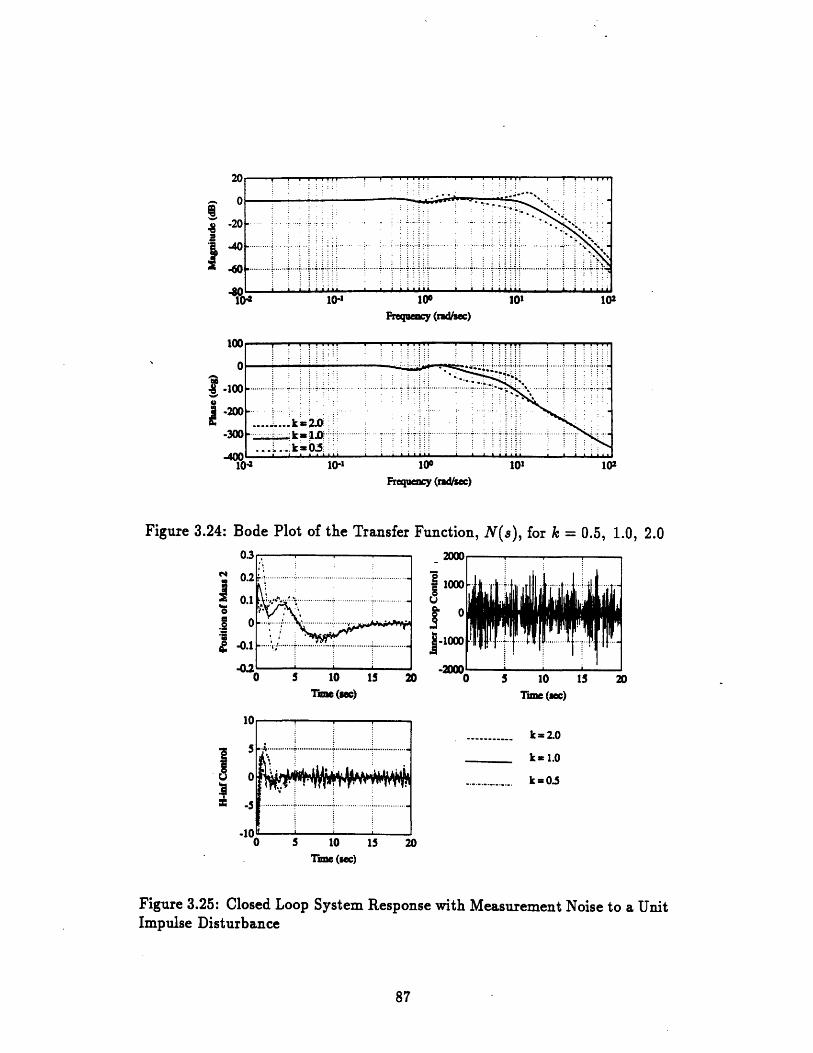
.0-20-- 4 0: : : . .. ... . .. ..... . . .. : ...... ... . .

,4 0 ........... ii i i i i!.... L. .. -i . i ....... .... ..., .. i.. .- ...; .. .• . ............. ... .....i... i. : .• ; ; i............ i.... .-•. ... .'. N.

.- 2 ...?. ..... i. ..i : . ... .

_llnl • i iii l l l l , i i i i l i i I : :;• J |

",04 d10 100 101 10

Frequency (rd/sec)

011

-200 k.... .. k• - •.

... ... ... .... ........ -..-.....-, •-.............. ..... .. . ..-S.i= 0.

100Frequency (rausec)

Figure 3.24:

I

Bode Plot of the Transfer

0.3

' '0 .2 -i.. .... ..... .. ........ ..... ..... .. .....0 .1 ...... ......... ........ ....... ........ ........ .......0 ............. .............. ; ......;.0 .1 ................ ............... .............-0.

0 5 10 15 21Time (we)

019

_1

0 5 10Time (sec)

Function, N(s), for k = 0.5, 1.0, 2.0x0n

100

.-10

0 5 10Time (sc)

I.

15 20

k = 2.0

k= 1.0

k = 0.5

15 20

Figure 3.25: Closed Loop System Response with Measurement Noise to a UnitImpulse Disturbance

87

.:

! l '

__

i.u

---- I , i I

amplitude. The disturbance is modeled as

w(t) = 1.0 sin(0.5t).

The response of the system to this disturbance is shown in Figure 3.26. The

compensated system attenuates the disturbance by approximately a factor of

one half over the full range of parameter uncertainty. The asymptotic settling

time of the system to the disturbance is less than 20 seconds for the full range

of parameter uncertainty, thus meeting the Design 2 specification.

The effects of measurement noise in this case are much the same as for the

impulse disturbance considered above. Therefore, the case of the sinusoidal

disturbance with measurement noise will not be considered here.

While not explicitly called for in the design specifications, the command

following performance of the control system is of interest. It is explored here

through the use of a unit step change in the reference. The response is shown

in Figure 3.27. Response is characterized by a very large overshoot of approxi-

mately 50%. This is due to the peaking found in the closed loop response bode

plot. The control efforts of both compensators are also large. This indicates

the nominal 'design does not have good command folowing performance. Inter-

estingly, Figure 3.27 indicates that the system is robust in terms of command

following performance. Therefore, though it was not done, constructing a new

H, compensator could possibly improve command following over the range of

parametric uncertainty.

3.4.6 Hoo Compensator Order Reduction: Design A

The approach to the Hr compensator reduction outlined in Section 2.6 was

used to reduce the H, compensator from 9 states to 4 states using the Schur

model reduction technique. The bode plot of the reduced order H, compen-

k-/V··j· .r -

20 30 40 0 10 20 30 40


k = 2.0

k = 1.0

k = 0.5

10 20 30 40Time (sec)

Figure 3.26: Closed Loop System Response

1.5I:1>;...I ....... .. .......

- 10 iS

Time (asc)

60

40

20

0

-20 ..... .......

.,AA L , '

to a Sinusoidal Disturbance

1 u

50

0 .

,

0 5 10 15 20Time (sec)

k=2.0k = 2.0

k = 0.5

5 10 15 20Time (sec)

Figure 3.27: Closed Loop System Response to a Unit Step in the Reference

89

0.5

2_

0

1 · ·

°L

) I

hr

I 1 I

.. .. ... .

.. ... .. ... ... . .... . .

MM"

.. : 1..1

~~ R

sator, Kr is indistinguishable from the original H, compensator. The infinity

norm of the difference between the compensators (equation 2.43) is equal to

0.096. The state-space realization of the reduced order compensator is given

in Appendix B.1.2.

The root locus plots of the closed loop system as k varies is shown in Fig-

ures 3.28 and 3.29. These indicate that the robustness of the system with the

reduced order compensator is identical to that of the full order compensator;

in fact, the reduced order compensator stabilizes the plant over the same range

of k as the full order compensator. The set of frequency response, and time

domain response plots for the system with the reduced order compensator are

identical to those of the original compensator indicating performance and ro-

bustness have been maintained. The entire set of plots and tables presented

above may be found for the reduced order compensator in Appendix C.

3.4.7 Summary of Design A

The system of compensators consisting of an inner loop and reduced order H,

compensator were used to provide a "solution" for the benchmark problem.

The compensators met the following design objectives:

* The closed loop system is stable over more than the full range of param-

eter variation, for 0.24 < k < 3.78.

* For a disturbance consisting of a unit impulse at time zero, the position

of mass 2 (the performance variable) has a settling time of less than 15

seconds for the full range of parameter variation.

* For 0.5 < k < 2.0 the system has phase and gain margins of

30.08 < PM < 56.88

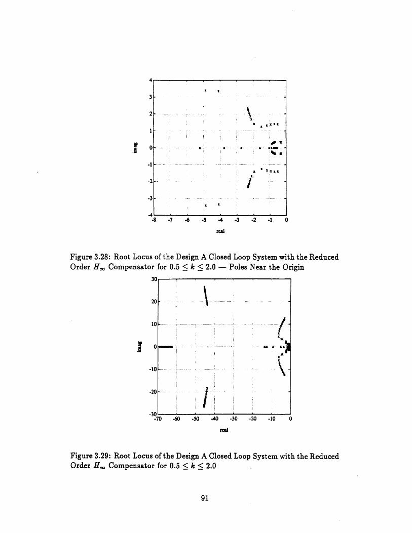
I

-8 -7 -6 -5 -4 -3 -2 -1 0

Figure 3.28: Root Locus of the Design A Closed Loop System with the ReducedOrder H, Compensator for 0.5 < k < 2.0 - Poles Near the Origin

-70 -60 -50 -40 -30 -20 -10 0

ral

Figure 3.29: Root Locus of the Design A Closed Loop System with the ReducedOrder H, Compensator for 0.5 < k < 2.0

91

a a ...• rIr I

U.

/£

20

-10

-20

...................... 1-1

... 1II

n-

I... ... .. .. .... . . . !... .. .. .

_ · · · ·

I N I 8 I I_]U - .

· ·

... .....

JU · -· · ·

.... .....

.. .... .

1

-

-I

.. .. ...... ..

1.91 < GM < 7.74

* For a sinusoidal disturbance with a frequency of 0.5 rad/sec the com-

pensated system will attenuate the disturbance by a minimum of nearly

50% regardless of the parametric variation. Again, regardless of the pa-

rameter variation the disturbance will be asymptotically rejected in less

than 20 seconds.

The following design objectives were not fully met.

* The controller effort was large in response to the impulse disturbance

and measurement noise. However, the impulse response effort would not

present a problem as the large control effort was of very short duration;

in an actual system it probably would not saturate the actuator. The

results of measurement noise are slightly more problematic. Because

of the large phase loss in the plant, lead compensation, which leads to

measurement noise amplification, is required.

* Measurement noise was not attenuated until almost a decade past the

closed loop bandwidth of the system. This is due to the large lead in the

inner loop compensator.

* The compensator system (K,. and Kinner) is an 8-state system, twice the

order of the plant. It is a complex compensator and this is an inherent

property of the methodology. The methodology trades off compensator

complexity for performance.

The compensated system met most of the design requirements and overall

the methodology was successful. Of the requirements not met the compensator

complexity is an inherent drawback of the methodology, one that is traded for

compensator performance and relative ease of design. The high lead compen-

sator that resulted is a product of the plant dynamics. Noise might cause an

actuator to "bounce" between its positive and negative limits. It is recom-

mended that, in an actual implementation limits be placed upon the inner

loop control magnitude to limit the large actuator commands.

The use of such limits on the inner loop actuator was investigated for a

unit impulse disturbance. A nonlinear simulation of the plant, inner loop com-

pensator, and reduced order Hl, compensator was constructed for k equal to

1.0. The effects of the impulse disturbance were evaluated for the nominal

system and for the system with limits of ±100 on the inner loop compen-

sator signal u,. A comparison of the two simulations is shown in Figure 3.30.

The figure shows that the inner loop limits cause a dramatic reduction in the

0 10 20

00-500 ...................... - . ........

.... Nomial0001

0 10 20 30Time (sec) Time (sec)

aL)

0 0.5 1 0 10 20 30Time (sec) Time (sec)

Figure 3.30: Comparison of the Nominal System and the Limited Inner LoopControl System to a Unit Impulse Disturbance

disturbance attenuation. While the settling time of the system still remains

within 15 seconds. An examination of the inner loop compensator effort for

both the sinusoidal disturbance and reference step simulations shows that the

inner loop compensator effort does not exceed L100, so these would not be

93

.2U

12gJu

Slo. ..-.. ..... .... ...- .-... . ... ...5001

5M , ... ..... .......·- · ·· ·-· · ·-0 Ino.o

._oo -

4

PM

-U

T~e~sc) T~~sec

• Jl. •."LJI.J

affected by the limits. Therefore, the effects of large control efforts by the in-

ner loop could be handled with nonlinear design techniques such as the limits

used here. More sophisticated approaches could also be used such as limit-

ing the output of each lead-lag in the inner loop compensator independently.

However, the design of such nonlinear "fixes" and their use under a variety of

inputs is beyond the scope of this study. The example given here is intended

to show that the high gain compensator resulting from the methodology can

indeed be implemented.

3.5 Compensator Design B

In this case an inner loop compensator was designed to remove the parametric

uncertainty without specifically attempting to retain the double integrator

characterisic of the plant. Since the benchmark problem has no requirements

on command following, only disturbance rejection at low frequency, this should

not pose a problem. However, the H, design will include an integrator to

facilitate command following and ensure that the DC gain of the closed loop

system T(s) is equal to one regardless of the value of k.

3.5.1 Constructing the Inner Loop Compensator: De-

sign B

Following on the guidelines given in Section 3.4.2, that is not allowing the

magnitude of the desired plant to exceed that of the actual plant, the desired

plant chosen here has the transfer function

(1.414)2(0.6)2() + 1.414)2(S + 0.6)2

This has the bode plot shown below in Figure 3.31, which also shows the actual

plant. Note the magnitude of the desired plant is always less than that of the

actual plant.

10

-100

10-2 10-1 10o 10' 102Frequency (r-d/se1)

-300 _ _

.2004 .. ... _......_..... . . -. . ... ... . . ... ... .. ... ... ... ... ... . ...... ... ... |.|... .. ..... .. ... .....

10-2 10-1 10 101 102

Frequency (rad/sec)

Figure 3.31: Bode Plots of the Desired Plant, Hd(s), and the actual plant G(s)

This yields an ideal compensator which is shown as a function of frequency

in Figure 3.32. The ideal compensator appears to be a lead network requiring

three or four lead components. After trying several compensators of different

order, a third order numerator design was settled on. While the design objec-

tives were achievable with both third or fourth order numerators, a third order

numerator was chosen in an attempt to reduce the compensator magnitude at

high frequency and limit noise amplification. The poles of the compensator

were iterated upon several times. The intention was to place them at a high

enough frequency so that they do not interfere with the compensator function

in the frequency range of interest; yet roll off the compensator to the extent

possible. This is the reason why the denominator has a higher order than the

numerator. A key advantage of using this methodology is demonstrated here,

95

iIn

--- ·:--- -·------.-...... ~ :.. :. - -·.~.--;...... -.............-. ~~ ..

...,.,.;.;.... . .....:....... ......:. -._ ...:...........................:.._._ ... :...~ ..... _..... ...,... :.

180 .11405

1601- ... ... .. .. .. ... . 360

1401- . 315

120 - 7 -270

100 -225

80 -180100. . . ...... ......... .... ......... 2

60 : .. 135

b 0 -e- 45

o PHASE( ideg) . j-20 ". 45

10-2 10-' 100 10' 102

Frequency (rad/sec)

Figure 3.32: Bode Plot of the Ideal Compensator, Kideal(S)

i.e. the ability to choose the compensator structure, order and complexity to

obtain the design goals. The structure of the selected compensator was fixed

to be(a3s3 + " + Cao)

(.02s + 1)2(.03s + 1)2

The methodology has built-in flexibility to minimize the difference between

the closed loop transfer function, Tinner and the desired closed loop transfer

function H based on a least squares fit of a0, al, a 2, a3. Thus, using a frequency

vector from 0.1 to 10 rad/sec, yields a compensator of the form

0.9883(3.687s + 1)(1.692s2 + 1.215s + 1)Kinn,,,() = (.028 + 1)2(.03a + 1)2

Examining the closed loop poles and their damping ratios and frequencies,

in Table 3.6, shows that the damping has been increased substantially from

the uncompensated plant. Notice as k increases from 0.5 to 2.0 a set of poles

migrates from the real axis towards the imaginary axis. At k equal to 2.0 these

96

poles have a damping ratio of only 0.1925 at 12.8 rad/sec. The decision has

been made to trade off this damping and gain margin for reduced magnitude

of the compensator at high frequencies.

k = 0.5 k = 1. _ k = 2.0Poles W ( P,les (C Poles w (

-0.3879 .3879 1 -0.3703 .3703 1 -0.3637 .3637 1-.7622-.5303j .9285 0.8209 -.539-.4908j 0.729 0.7394 -. 4919-.4818j .6886 0.7144

-. 7622+.5303j .9285 0.8209 -.539+.4908j 0.729 0.7394 -.4919+.4818j .6886 0.7144-2.394 2.394 1 -5.179-7.641j 9.231 0.5611 -2.47-12.59j 12.83 0.1925-12.07 12.07 1 -5.179+7.641j 9.231 0.5611 -2.47+12.59j 12.83 0.1925

-43.87-18.63j 47.66 0.9204 -44.59-22.46j 49.93 0.8931 -45.51-26.78j 52.8 0.8619-43.87+18.63j 47.66 0.9204 -44.59+22.46j 49.93 0.8931 -45.51+26.78j 52.8 0.8619

-62.56 62.56 1 -65.67 65.67 1 -69.36 69.36 1

Table 3.6: Closed Loop Poles of Tinner: Design B

Examining the root locus of Tnner, Figure 3.33, shows that a pole pair

begins real for k equal to 0.5 and moves towards the imaginary axis as k

increases. This is the pole pair referred to above.

3u

10

-20

30r-70 -60 -50 40 -30 -20 -10 0

Figure 3.33: Root Locus of the Closed Loop System, Tij,,n(s) for 0.5 < k < 2.0

The open loop bode plot, shown in Figure 3.34 reveals that the systems

have a wide range of crossover frequencies for varying k. The closed loop bode

..a.·-··IL · ·

.

.. ...............

.. .. ...... .. ... .. ...

....... .......

I

................. ...........'"

... ... .. ................

m I I I i A I . .1.... v

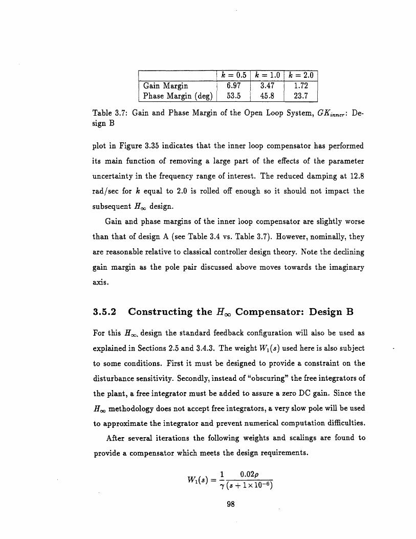
Table 3.7: Gain and Phase Margin of the Open Loop System, GKinner: De-sign B

plot in Figure 3.35 indicates that the inner loop compensator has performed

its main function of removing a large part of the effects of the parameter

uncertainty in the frequency range of interest. The reduced damping at 12.8

rad/sec for k equal to 2.0 is rolled off enough so it should not impact the

subsequent H, design.

Gain and phase margins of the inner loop compensator are slightly worse

than that of design A (see Table 3.4 vs. Table 3.7). However, nominally, they

are reasonable relative to classical controller design theory. Note the declining

gain margin as the pole pair discussed above moves towards the imaginary

axis.

3.5.2 Constructing the Hoo Compensator: Design B

For this H,. design the standard feedback configuration will also be used as

explained in Sections 2.5 and 3.4.3. The weight W (s) used here is also subject

to some conditions. First it must be designed to provide a constraint on the

disturbance sensitivity. Secondly, instead of "obscuring" the free integrators of

the plant, a free integrator must be added to assure a zero DC gain. Since the

H, methodology does not accept free integrators, a very slow pole will be used

to approximate the integrator and prevent numerical computation difficulties.

After several iterations the following weights and scalings are found to

provide a compensator which meets the design requirements.

1 0 .0 2pS- (r + 1 x 10- 6 )

98

Ooen Loon

System

•O-2 10-1 10P 10'

Frequency (mds)

-100

-3 102

Frquency (rad/sc)

Figure 3.34: Bode Plot of the Open Loop System, GKinner

4A ,Closed Loop System

-100

-150

-'nfl.2

Frequeacy (mdsec)

Frequcy (rad/sec)

Figure 3.35: Bode Plot of the Closed Loop System, Ti,,er

99

% WPIF. L.WVLJ OVOLU.100

...... .... .......... .. ....

...... ......... ... ..... .. ... .... .. ... .... ... ... .. .... .. .... ... . ... ... ... ..

-1001 1 1 1111111 I 1 1111(11 1 1 1111I1I L 1 1111 a

I.... ... . .. .... .... .. ..... .. .

.. . .. . ... .. . .... .. ..... . .. .... .... .

..

.

.

..

II I [ . ... . . . . -- - -- .

5ur

--

ii. . . . . .| A . . . . . . . . . & • | | I

10

10

1W2(s)= 0.02

W 3 (s) = -S 2

The near optimal H'o compensator found had scaling values of

p = 28,

7=1.

The bode magnitude plots of the inverses of the weights and the sensitivity

specification, Wi(s) are shown in Figure 3.36.

80

60

40

20

0

-20

-40

-60

-80

-100

-12010"2 100

Frequency (radsec)

Figure 3.36: H. Design Weights and Actual Sensitivity Specification

The compensator obtained is shown in Figure 3.37; it is very similar to the

compensator obtained in design A with the addition of the low frequency pole

approximating an integrator. The state-space realization of the compensator

is given in Appendix B.2.1.

100

........... ....... ........... · ................. ...... ..... .. . ...... .... ... ........ .. ...... .... ... ......

.. .. ... ..... .· · · · · ·· · ·. .. . .. .. ... ..~~~

... ... ..

................ .. .... ........ . ...................4......................

......... , .......... ... .... ..

---vf ....: .... ... .......... ............. ...................._.;.../j MUS)I

C

60 315

db 0 180

40- 45

-8 0 ............. .............................. ...... ........ O d eg

-100 ..- 45..... ... ........ . .....

-120 -90-140 135(deg)

10-2 10-1 100 101 102

Frequcy (rad/sec)

Figure 3.37: Bode Plot of the H, Compensator

The compensator provides a stable closed loop system over the full range

of parameter variation. The range of k for which the closed loop system is

stable is

0.21 < k < 3.42.

The closed loop poles are reasonably well damped in the frequency range

of interest for the full range of k. This is illustrated by the root locus in

Figure 3.38; note one pair of the complex poles has decreased damping as k

goes from 1 to 0.5.

3.5.3 Frequency Response of the Compensated Sys-

tem: Design B

The bode plot of the open loop system, G(K, + Ki,,,,,), is given in Figure 3.39.

As expected, it is very similar to Figure 3.19 for Design A. Interestingly the

magnitude plot crosses over at less than -20 dB/decade.

101

-8 -7 -6 -5 -4

rel

-2 -1 0

Figure 3.38: Root Locus0.5 < k < 2.0

of the Plant with Inner and H. Compensators for

100

Froquency (ra/sec)

Frequency (rad/sec)

Figure 3.39: Bode Plot of the0.5, 1.0, 2.0

Open Loop System G(Kinner + Ko) for k =

102

.. f...

101

AI4 F I L II

.4 i i i i l i ,I

il

. .................. ............ ..... ...... ............ ......... ......-.....:... .... . ..........

a m

-.... · ...··........ ......... ....................... ..... ·... '..... ... ... ... ... .... ... .. ... ... .. ... ... .... . .. ...

-1l0l

The gain and phase margins of the open loop system are shown in Table 3.8.

The margins are slightly degraded from Design A but provide reasonable sta-

bility robustness. The same trends as in Design A are present, though in this

design phase margin continues to increase as k decreases.

k = 0.5 k = 1.0 k = 2.0Gain Margin 6.99 3.48 1.73Phase Margin (deg) 52.9 46.3 23.9

Table 3.8: Gain and Phase Margin of the OpenDesign B

Loop System, G(Ki,.er + Ko,):

The closed loop bode plot is shown in Figure 3.40 and varies from that in

design A. It has slightly less bandwidth, 0.9 rad/sec versus 2.4 rad/sec, but

does not have the peaking of Design A which contributes to this increased

bandwidth. The closed loop shape for design B is better from a command

following viewpoint.

-50

-100

-150

_.1'l100

Frequency (vd/ftc)

-100

-200

-300

10-2 104- 10 101 102Frequency (rad/sec)

Figure 3.40: Bode Plot of the Closed Loop System T(s) for k = 0.5, 1.0, 2.0

103

A

10-o

.. .. ... .. ... .... .. ..... .. .. .. ..... .... ....... ..... ... .... ... .......... . . .. .. ... ... .... ..... ..... .... .. .. .... ... .....

........ k=2.0i

. 2: . ·

Or

I - . . . .- . . .. . . . . . . . .%J

Ur

WWWII

716ý.. .. ... .. ........ ... .. ... ..... .. ... .... .. .... ... ... ... .. ... .

Again the sensitivity transfer function is of great importance and its bode

plot is shown in Figure 3.41. Disturbances are attenuated past 2 rad/sec for

the nominal case (as for Design A) and past 1 rad/sec regardless of the value

of k.

O0

E -50

1 -100

1 0I10-2 10-1 100 10' 102

Frequency (rad/ec)

.20 0 - . . ..... . ... . ..... .... .. . ..........

A. . ........ ...

S .... ... .. i ...... .... . .... ........ .. .. ..

... .. k 0:008 1 1 • l , t t t t t * IIII

10- 2 10-1 100 10' 102

Frequency (rad/sec)

Figure 3.41: Bode Plot of the Sensitivity Transfer Function S(s) for k =0.5, 1.0, 2.0

The transfer function from the design disturbance w to z is shown in Fig-

ure 3.42. It appears that Design B should also do a good job in rejecting w,

as w is attenuated over all frequencies.

Finally, it is of interest to check the noise transfer function, N(s). It is

shown in Figure 3.43 and is very similar to that of Design A. This design will

also have poor noise attenuation.

Based on frequency response analysis it appears that the combination of

inner loop and H, has yielded a compensated system which will successfully

meet most of the design requirements.

104

---

-·

-4

-6

-R

0

0o0

n10-2 10-' 100 101 102

Frequency (rad/sec)

2Rv

-200

-400

6- 0

Frequency (rad/sec)

Figure 3.42: Bode Plot of the Transfer Function from w to z for k =0.5, 1.0, 2.0

0

-20

-0 ..... ....... .. .. ...10-2 10-1 100 101 I02

100-

0100 .. .. . ..... ... ..... ..... ..

Frequency (rad/sec)

Figure 3.43: Bode Plot of the Transfer Function, N(s), for k = 0.5, 1.0,2.0

105

e- ···- ··- · ·· ·· · -.. ··.. ....... ..... .....I··-· · ··; · ·i- · · · ··· · ··

S -............

... ..k=03'

VV I

-1

"V At -- - - - - . . . .

lvv

V

3.5.4 Time Response of the Compensated System:

Design B

The time response of this system to a unit impulse disturbance w is shown

in Figure 3.44. Again both the performance variable z and the controls are

presented. The response is very comparable to design A (no surprise based

on the comparative frequency responses). The performance variable z has a

very similar trajectory, meeting the specified requirements for the entire range

of parameter variation. The inner loop control again has a very large initial

response to the disturbance.

0. 1 ... ..0 .0... .......

0

0.3 1000

0.2 .. a 500,- _ . i.• -

0. U.3

A0 S 0 iS 20 0 5 10 15 20 5 10 15 20 0 5 10 15 20


k = 2.0

k = 1.0

k . . 0.5

0 5 10 15 20Time (sec)

Figure 3.44: Closed Loop System Response to a Unit Impulse Disturbance

In general, the time response of Design B is very similar to Design A, except

for the step response. The step response shown in Figure 3.45 has very little

overshoot and rise times of less than four seconds regardless of the value of k.

The command following performance of the system is robust to the parameter

variation.

106

1 , ,

rr

k.c

... .................

As stated above, the remainder of the time response is very similar to

Design A and so it is presented without comment in Figures 3.46 and 3.47.

Overall, the time response of the compensated system meets the require-

ments of Section 3.2 and provides excellent command following performance,

over the entire range of parameter variation.

3.5.5 H,, Compensator Order Reduction: Design B

Again the technique of Schur model reduction was applied to the H, compen-

sator. The resulting reduced order compensator has six states (versus nine)

and its state-space realization is given in Appendix B.2.2. The bode plot of

the reduced order compensator is indistinguishable from that of the full order

compensator. The infinity norm of the difference between the compensators

is equal to 0.023.

The root locus plots of the closed loop with the reduced order compensator

are shown in Figures 3.48 and 3.49. Stability over the full range of parametric

uncertainty is unchanged with the reduced order compensator. Performance

with the reduced order compensator is indistinguishable from that of the full

order compensator. The figures containing the system performance with the

reduced order compensator are shown in Appendix D.

3.5.6 Summary of Design B

The compensator system designed provides excellent performance and sta-

bility robustness to the full range of parameter variation. The compensator

system provides Type 1 system response for the closed loop system and met

the following design objectives.

* The closed loop system is stable over the entire range of parameter vari-

ation. The range of k for which the system is stable is 0.21 < k < 3.42.

107

0 5 10Time (sec)

30

20

10

0

-10

-200 5 10

Time (tec)15 20

k = 2.0

k = 1.0

k = 0.5

0 5 10

Time (sec)

Figure 3.45: Closed Loop System Response to a Unit Step in the Reference

'3.

0.2

0.1

0

-0.11CI 5 10

Time (sec)

2 1000

. 0

ý.Y " 1-1000.........

-200015 20 0 5 10 15 20

Time (sec)

k = 2.0

k = 1.0

k = 0.5

Time (sec)

Figure 3.46: Closed Loop System Response with Measurement Noise to a UnitImpulse Disturbance

108

II

....-....... ... ............. ........ ..... ..

... ... .... .. ................. .......... ...... .........

II

I)

.................. ......... ............^... ..................

.. .... .. . ... .. ... .

.

eq

' 0.0

0j04

In

0

0.

j

0 10 20 30 40 )


0.5-

o ·· ·

-0 .5 ..... ... .......·--:' ······-

-k = 2.0

k= 1.0

k= 0.5

0 10 20 30 40Time (sec)

Figure 3.47: Closed Loop System Response to a Sinusoidal Disturbance

* The system attenuates a unit impulse disturbance to at least 25% of the

input magnitude. The system has a settling time of less than 15 seconds.

This is regardless of the value of k.

* The sinusoidal disturbance is attenuated by more than 50% and is asymp-

totically rejected in less than 20 seconds regardless of the parameter

variation.

* The performance variable response to a step change in the reference has

characteristics of a 4 second rise time and almost no overshoot, regardless

of the parameter variation.

* The system has phase and gain margins of

23.92 < PM < 52.85

1.73 < GM < 6.99

109

9N r 7 1 1~·. ,I'

r,

-8 -7 -6 -5 4 -3 -2 .1 0

Figure 3.48: Root Locus of the Design B Closed Loop System with the ReducedOrder H.. Compensator for 0.5 < k < 2.0 - Poles Near the Origin

20

-10

-20

-60 -50 -40 -30 -20 -10real

Figure 3.49: Root Locus of the Design B Closed Loop System with the ReducedOrder H. Compensator for 0.5 < k < 2.0

110

......... ... .• . , -~ ~ ~ ~~ .... .... . .. . ............. i.... .......... ............*u im 1.

a

I

.. . .. ....................... ... ......... ............. .I . •..... .... !

.. . ........: ........... ... ;........... . .. "/ .-· · · · · · ·· · ·· ·- · · ·- · · + II

4.

Y i i i I i , I i

1'·

.lr

. .. . . . . . .

.. ..

.. .... .. . . .... .......... .. .. ...... .......

-

..... ..... . .... ......... ...

n l ... . . .. ....... . .

•. . .. ... . ........... . . .

for 0.5 < k < 2.0.

The following objectives were not fully met.

* The controller effort was large in response to the impulse disturbance

and measurement noise (re: discussion in Sections 3.4.5 and 3.4.7).

* The compensator system is complex, consisting of a four state inner loop

compensator and a six state H, compensator, a total of ten states.

* Measurement noise is not attenuated till almost a decade past the closed

loop system bandwidth.

The compensated design met the performance objectives of the problem

using a complex, high bandwidth compensator system. The advantages and

disadvantages are discussed in Section 3.4.7.

3.6 Comparison to Published Results for a

Benchmark Problem for Robust Control

Five papers presented at the 1990 ACC [4, 6, 7, 17, 22] proposed compensators

to meet the requirements of this problem. A comparison with those papers of

the designs presented in this thesis elicits the following conclusions.

All of the papers stabilized the closed loop system over the range of param-

etric variation, 0.5 < k < 2.0, except [4] which was stable for 0.55 < k < 2.0.

The impulse disturbance time response of the designs presented here is

superior to all of the ACC designs except that by Chiang and Safonov [6].

The impulse disturbance response specifications are met by only [6, 7] for the

nominal case and only [6] over the entire range of parameter uncertainty. No

impulse response was presented for [22].

111

The only papers which investigated the sinusoidal disturbance were [6, 22],

with the design of Rhee and Speyer [22] designed specifically designed to reject

a sinusoidal disturbance at 0.5 rad/sec. Both designs met the requirements

with [22] completely attenuating the sinusoidal disturbance. Both designs

presented here also meet this requirement and effectively attenuate a sinusoidal

disturbance at any frequency.

The compensator designs presented here are of greater order than any of

the other designs with the exception of [22] which is an 8 state compensator.

Control magnitudes given in this thesis are greater than the control mag-

nitudes of the ACC compensators except for that of Chiang and Safonov [6]

which is a lead network with a high frequency gain of greater than 100 dB.

The problems that apply to the inner loop compensator due to its high gain,

will also apply to Chiang and Safonov's compensator.

The effects of measurement noise are only investigated by [22]. The noise

model used is Fv where r is 0.033 and v has unit covariance. This noise does

not appear to show up in the system output and has no significant impact on

the control effort.

The designs presented here have higher gain and phase margins than the

designs which tabulate their margins. All of the compensators except [6] were

nonminimum phase. Both compensators presented here are minimum phase.

This is important for implementation.

Overall the designs presented here compare favorably to the designs pre-

sented at the ACC. Both designs give better performance and stability margins

than most of the designs from the ACC. The designs presented here trade in-

creased complexity, controller effort, and noise rejection for the performance

gained.

112

Chapter 4

A MIMO Mass-Spring-Dashpot

Problem

4.1 Introduction

In this chapter the design methodology outlined in Chapter 2 and sucessfully

applied to Wie and Bernstein's SISO problem (Chapter 3) is applied to a multi-

input multi-output (MIMO) problem with parametric uncertainty. Again the

problem considered is a mass-spring problem, though in this case the problem

contains dashpots and so it is lightly damped. Here there are two inputs and

two outputs, with one set of sensors and actuators colocated and the other

non-colocated. The basic framework of the problem is set up as in Wie and

Berstein's and similar requirements will be applied.

4.2 The Plant: A MIMO Mass-Spring-Dashpot

(MSD) System

A schematic diagram of the plant can be seen in Figure 4.1 below. Here the

actuators of the plant (the inputs) are forces acting on m, and m 2 while the

113

plant sensors (the outputs) measure the positions of mi and m3.

Figure 4.1: Schematic Diagram of the MIMO Mass-Spring-Dashpot Plant

The state equations of this system may be expressed as

Y:2

£4

Y5

Y6

Z1 =

0

0

0

-(k+l 2+ks)ml

m 2

o o

o o

0 0

o j

o o0

0

0

0

mI

--(k3+k+kT)M 2m3M3

ulu2 -+-

0

0

m2

-(k 2+k 3 +kI6)m 3

0

0

0I

m2o

o 0

1 0

o 10

-(b2+b3) 0m2

0m 3

XL

X2

X3

X:5

L x:6

Z2 = X3

- 3 + v

114

14I

Where the variables are defined as:

m; = mass of body i

ki = spring constant of spring i

b; = damping factor of dashpot i

2X = position of body 1

z, = position of body 2



x5 = velocity of body 2


ul = control input (force) acting on body 1

u, = control input (force) acting on body 2

w = plant disturbance (force) acting on body 3

yj = measured position of body 1

y2 = measured position of body 3

zl = performance variable, position of body 1

z2 = performance variable, position of body 3

v = measurement noise

This problem is taken from [1].

Now for simplicity in handling the problem let

mi= m m 3 = m = 1

bl = b2 = b3 = = b = 0.002.

115

Let the nominal value of the spring constants be

with the parametric uncertainty manifested as a simultaneous variation in the

all of the spring constants such that

kl = ... = G = k

and

0.5 < k < 2.0.

Obviously, uncertainty in the value of the spring constants could result in

a large number of plant variations. This simultaneous variation is intended for

simplicity in handling the problem. No effort has been made to check whether

this represents a worst or best case in terms of plant variation and uncertainty.

The design specifications may be considered essentially the same as those

in Chapter 3.

4.3 Analysis of the Plant

The nominal plant has the singular value plot shown in Figure 4.3 and clearly

reveals the system has three pairs of lightly damped poles. The system has no

transmission zeros. As k varies the singular value plots at the extreme varia-

tions, k = 0.5 and k = 2.0, are shown in Figures 4.2 and 4.4. A comparison of

the maximum singular values as k varies is shown in Figure 4.5. The changing

value of k affects both DC gain and pole location of the plant. The gain varies

about 10 dB and the poles move about 1.5 rads/sec in frequency.

The nominal poles, natural frequencies, and damping ratios are tabulated

below.

116

-50-100 -

-20010-2 10-' 100 10' 102

Frequecmy (rad/sec)

Figure 4.2: Singular Value Plot of G for k = 0.5

> .100 .. 0. 1 101......k = 1.0

10-2 10-1 100 101 102

Frequency (rad/sec)

Figure 4.3: Singular Value Plot of G for k = 1.0

S-50

k = 2.0

:20010-2 10- 100 101 0 2

Frequec (rd/ac)

Figure 4.4: Singular Value Plot of G for kc = 2.0

. ...... .... ..... ............ ...... .......

--- -- -- - - - -- --- - - -- - -- - -- - - -:

-. ................100 .... . .. .O.. ..i i , i n; :,i . i i ii ,

10- 10-1 100 10' 1(

Fnque~cy (rad/sec)

Figure 4.5: Maximum Singular Value Plot of G for k = 0.5, 1.0, 2.0

117

Table 4.1: Poles of the Nominal MIMO MSD System

The locations of the poles are shown as a function of the spring constant,

k, in Figure 4.6 below. Note that varying k only changes the real part of each

pole, the imaginary part remains fixed.

II

-0.01 -0.008 -0.006 -0.004 -0.002 0

Real

Figure 4.6: Plant Pole Location for 0.5 < k <K 2.0

With this in mind an attempt will be made to design

pensator.

the inner loop com-

118

Pole ( w-0.001+1.000j 0.0010 1.000-0.001-1.000j 0.0010 1.000

-0.001+2.000j 0.0010 2.000-0.001-2.000j 0.0010 2.000

-0.003+2.000j 0.0015 2.000-0.003-2.000j 0.0015 2.000

4.4 Design of the Model-Matching Inner Loop

Compensator

The first step in designing the inner loop compensator is choosing a desired

plant, Hd. To assist in doing this it will be necessary to obtain bode plots

of the individual plant input/ouput channels. These are shown in Figure 4.7

for the nominal plant. Interestingly, channels G12, G21 , and G2 2 are identical

while G,1 has a higher DC gain and rolls off more slowly. Notice each transfer

function contains two pairs of lightly-damped poles and no zeros, except for

G11 which has a pair of lightly-damped zeros.

After several iterations a desired plant is chosen such that it mimics the

actual plant but has all of its poles on the real axis. The transfer function

elements of the desired plant were picked by moving the undamped poles of

the nominal plant to the real axis (at the same natural frequency) and choosing

the DC gain so the desired plant element's magnitude is less than the actual

plant element's magnitude over all frequencies, as per the SISO inner loop

designs. Except for the 11 channel where the plant has lightly damped zeros

and the desired transfer function omits both those zeros and a lightly damped

pair of poles. The desired plant, Hd, which meets the conditions above has

individual channel transfer functions of

_ =(0.5)(1.4142)2d (s + 1.4142)(s + 1.4142)

H12 = (0.2)(2)2

(S + 1)2(S + 2)2

21 = (0.2)(2)2d = (s + 1)2(s + 2)2

119

os.

*-1

cPI0 0d

j

0

-L

I

iW

-

C)

0

J

-cb~

Hlj ·

; C

)

§ I1

2·:

'

··

--;-

-....

= (0.2)(2)2S (S + 1)2(S 2)2

These transfer functions are shown in Figure 4.8, which compares the magni-

tude plot of each channel of the desired plant with the respective magnitude

plot of each channel of the nominal plant. This illustrates the points discussed

above.

50

dboL..

100 7-DesiredPat-No P

10-2 102

Frequency (=Wswe

10-2 102Frequency (rad/sec)

12

db O0

-50

-100-i .Desired Plant

-150 k Nominanul .....10-2 102

Frequency (rad/sec)

22

db 0

-50

-100.Desed Plant

-150 -- NomaM••Pian10-2 102

Frequency (ra/sc)

Figure 4.8: Bode Plots Comparing the Channels of the Desired Plant, Hd, tothe Nominal Plant, G

Computing the frequency plots of the ideal compensator, Kideat, (again,

channel by channel) from equation 2.29 yields the results shown in Figure 4.9.

The ideal compensator is similar to the SISO problem in being essentially a

lead network, or here, a set of lead networks. Obviously, this may cause mea-

surement noise problems. In any case it is desirable to have the compensator

design of the lowest order which effectively removes most of the parameter

uncertainty. After several iterations on compensator. order and pole location

121

..- 405

-360

S315

- . . 270

225

- 130

........ .. ...... . ........ 4.- ,o• . . .

O- 104' 1I 10' 1r--

12

104 lot

-7-geng NMV 10 -

10 10'"l"ip 10- 10 -Reqemcy (=dMs)

Figure 4.9: Bode Plots of the Channels of the Ideal Compensator, Kideal

122

60

40

20

00-20

-40

-40

-100

Wi60

40

-10

-40

-100

.........

MAEN

MIn

mIM. Int

- --

........... ............ . ....... ·· ·'·-..-r·....... ... .... ... ... .. ........... ... .. ..

. ... .. .....

...... ...... .. .... .....-·- - · ··· ·~-········-PRAE : ·f

"11

AIM • • _'m A almg

- fi"l • lqK

the model matching design method produced the following compensator:

0.976(2.755s + 1)K"

rner 0.01s + 1

K12 -1.193(2.769s - 1)inner 0.01s + 1

K 21 -1.178(2.819s - 1)inner 0.01s + 1

K 2 2-0.580(-33.49s + 1)(0.439s2 + 0.6598s + 1)Snenr (0.01s + 1)(0.01s + 1)(0.02s + 1)

The actual compensator has less lead than the ideal compensator. Chan-

nels 11, 12, and 21 each contain a lead-lag, while channel 22 has three lead-lags.

The design process showed that it is channel 22 which is crucial to the design.

The compensator poles were chosen to give causal compensator realizations

which would allow the desired transfer function Hd be attained, yet reduce the

effects of the large lead networks necessary at high frequencies. As can be seen

from the transfer functions, the poles had to remain at high frequency and the

channel 22 lead network is of large magnitude at frequencies above crossover.

The bode plot of each channel of the actual compensator, Kinner is shown in

Figure 4.10 and the compensator singular value plot is hsown in Figure 4.11.

When this inner loop compensator is combined with the plant, it yields

the closed loop poles, with respective frequencies w and damping ratios (, as

compiled in Table 4.2 for the standard values of k.

The inner loop compensator provides a closed loop transfer function, Tin,,r,

which is stable over the entire range of parameter variation. The damping

ratios of the closed loop poles are also substantially improved over those of

the base plant for the full range of parameter variation. The movement of the

closed loop poles as the spring constant varies, is shown in the root locus in

123

50-

0.

-50-

-10010-2 102

Frequency (rad/sec)

21

50

0

-50 --

-100 1

10-2 102

Frequency (rad/sec)

-50

-100

12

M r-1

I *1

~GN~rU:

10-2 102

Frequency (rad/sec)

22150 7-7

100 -

50 -

0-

10-2 102

Frequency (rad/sec)

Figure 4.10: Bode Plots of the Inner Loop Compensator, K,,,,,er, Channels

Figure 4.11: Singular Value Bode Plot of the Inner Loop Compensator, Kinner

124

k = U.5 k = 1.( k = 2.0

'Iies .~ Pol es ! ,•es I C-0.2168 .2168 1 -0.5862 .5862 1 -.4083-.8373j .9316 .4382-0.5658 .5658 1 -.8103-.7179j 1.083 0.7-185 -.-I083+.8373j .9316 ..1382

-1.321 1.321 I -. 8103+.7179j 1.083 U.7-185 -1.315 1.315 1-1.528-1.438j 2.098 0.7282 -1.47-1.089j 1.829 0.8036 -1.397-2.299j 2.69 .5194

-1.528+1.438j 2.098 0.7282 -1.47+1.089j 1.829 0.8036 -1.397+2.299j 2.69 .5194-2.518 2.518 1 -15.37 15.37 1 -12.41-20.56j 24.01 .5168-36.12 36.12 1 -17.47 17.47 1 -12.41+20.56j 24.01 .5168-97.22 97.22 1 -97.22 97.22 1 -97.23 97.23 1

-10,t.5-18.04j 106 0.9854 -107.4-23.69j 110 0.9765 -111.5-30.4-7j 115.6 .9646-104.5+18.04j 106 U.9854 -107.4+23.69j 110 0.9765 -111.5+30.47j 115.6 .96-16

Table 4.2: Poles of the Closed Loop System, Tinner, k = 0.5, 1.0, 2.0

Figure 4.12. This is the root locus of the poles of Tinner, obtained by varying

the spring constant, k, in the closed loop A matrix, as were those shown for

the benchmark problem.

30

-10

-20

-120 -100 -80 -60

real

-40 -20 0

Figure 4.12: Root Locus of the Closed Loop System, Ti,,nner, for 0.5 < k < 2.0

The next three figures show the open loop singular value plots of the sys-

tem, with the loop broken at the plant output GKinner, for the standard values

of k. Figure 4.13 shows k = 0.5, Figure 4.14 shows k = 1.0 and Figure 4.15

shows k = 2.0. Figure 4.16 compares the maximum singular values of each.

125

*· ..I.. *. *1**i

AA

-4Ul

J•

-

e

+

IArn

LJ

Frequency (rad/sec)

Figure 4.13: Open Loop Singular Value Plot of GKinner for k = 0.5

Frequency (rad/sec)

Figure 4.14: Open Loop Singular Value Plot of GK,,nne, for k = 1.0

U

Frequency (rad/sec)

Figure 4.15: Open Loop Singular Value Plot of GKinne,r for k = 2.0

Frequency (rad/sec)

Figure 4.16: Open Loop Maximum Singular Value Plot for k = 0.5, 1.0, 2.0

126

Similarly, the closed loop, Ti,,,,r, singular value plots are contained in Fig-

ure 4.17, Figure 4.18, Figure 4.19 and Figure 4.20. The inner loop compensator

has successfully removed a large amount of the plant variation generated by

the parametric uncertainty, the poles are well damped and the remaining un-

certainty consists of varying DC gain and system bandwidth. Since the DC

gain of Ti,,,,r still varies with k, the H, compensator will be augmented with

an integrator to eliminate this in the final closed loop transfer function, T.

The system is amenable to stable H, designs over the range of parametric

uncertainty.

4.5 Design of the H, Compensator

The design of the H, compensator begins with the selection of weights. In

this problem, as before, W1i(s) will be used to provide not only disturbance

rejection but integrators to provide a DC gain of one in the closed loop system

regardless of the value of k. The integrator, again approximated as a very slow

pole, will also provide zero steady state error to any commanded reference in-

put. Since the closed loop sensitivity of the entire system will differ from that

as constrained by Wi(s), as explained in Section 2.5, it must be chosen care-

fully. W3 (s) will provide a limit on the closed loop bandwidth of the system,

it is chosen to provide reasonable time response without unduly extending the

closed loop bandwidth. If the closed loop bandwidth were overextended, it

could have negative implications for both performance and stability robust-

ness. Finally, W2 will be used to guarantee that the augmented plant, P',

meets the requirements of the H_ methodology.

The weights chosen after some iteration were

0.2p 0

W1 1(s) = 8+0.00000S 0 +.2pY+o.O{_}OOUl

127

Frequency (rad/sec)

Figure 4.17: Closed Loop Singular Value Plot of Tinnr, for k = 0.5

----------- ------------------

-50

"- .. . . . ... ... ...... ...... ... ..... ....... .. .. . ........-100

-150 .........

-20010-2 10- 100 101 102

Frequency (mad/sc)

Figure 4.18: Closed Loop Singular Value Plot of Ti,,,, for k = 1.0

.. ..... . -. ... .... ..S•100 . . ....

.20 . . .. ......... . .10-2 10-1 100 10 102

sequency (rd/isc)

Figure 4.19: Closed Loop Singular Value Plot of Tinn,, for I = 2.0

20

2 0 -. .... . . .. ........ ...... .. ..-20 > 40-

Max SV

-80 =.10-2 10-1 100 101 102Frequency (rad/sec)

Figure 4.20: Closed Loop Maximum Singular Value Plot for k = 0.5, 1.0, 2.0

128

1W>=

-Y

T4'i(s)__1

-Y

0.02 0

0 0.02

0.5s' 0

0 0.5s2

Where, in the compensator chosen,

p = 3.8

-7=1.

These parameters were chosen by fixing y, and, thusly, the closed loop band-

width of the system, and then varying p until the sensitivity function is nearly

minimized in the frequency range below crossover. The bode magnitude plots

of the diagonal elements of the weights are shown in Figure 4.21 along with

the constraint implied on the actual sensitivity function, W,'(s).

The singular value plot of the compensator obtained from these weights is

shown in Figure 4.22. The integrators are apparent in the plot of the com-

pensator. The compensator has a large magnitude across the frequency range

of interest (the frequencies around the open loop crossover frequency). The

state-space realization of the compensator is given in Appendix B.3.1.

4.6 Analysis of the Closed Loop System

The closed loop system, T(s) is stable over the entire range of parameter

variation, 0.5 < k 2.0 and is stable over a range of

0.21 < k < 7.89.

129

UJ

20

-20

-AA

10"

Frequency (rad/sc)

Figure 4.21: Bode Plots of the H, Weighting Functions, Wi(s) and W3(s),and the Implied Constraint W:(s)

Figure 4.22: Singular Value Plot of the Hc Compensator

130

.-•.· i ' " . - 1/Wi (s) .

,. /W1.(s)I ·-------- Ir/wFlpc s

.. .

~.·~: · ·

2

,.,,,,,.,,,,,

I:

-

The movement of the poles with k is illustrated by the root locus in Figure 4.23.

Closed loop damping decreases as k varies from its nominal value. A survey of

the minimum damping ratios and their associated natural frequencies among

the closed loop poles for the three standard values highlights this fact. The

data is presented in the table below, Table 4.3.

20

-10

-20

-30

-AA-120 -I00

Figure 4.23: Root Locus of the2.0

-80 -60 -40 -20 0

Poles of the Closed Loop System for 0.5 > k >

k = 0.5 k = 1.0 k = 2.0Minimum 4 0.2712 0.6356 0.3839w 1.086 2.165 1.232

Table 4.3: Table of the Minimum Damping Ratio of the Closed Loop Poles

Figure 4.24 shows the effect on the minimum damping ratio of the low

frequency poles of k varying from 0.5 to 2.0. The performance degradation as

k varies will be more pronounced than in the SISO. case due to these under-

damped poles at low frequencies.

131

:7\j...................... 19 .....~~· ~ ~ ~ ~ ... ·.. .... ...-

. ..

40

Figure 4.24: Minimum Zeta of the Closed Loop System as a Function of k

The gain and phase margins of the closed loop system are presented in

Table 4.4. The system demonstrates good stability margins for the entire

range of parameter uncertainty. Furthermore, it must be remembered that:

* This is a conservative measure of stability (See Section 2.2).

* The optimal values are obtained by taking the oo-norm of the sensitivity

function equal to one and substituting it into the definitions for the

gain/phase margins, equations 2.7, 2.8, 2.9.

IGain Margin = 1

TGain Margin = oo

Phase Margin = 60 degrees

132

k = 0.5 k = 1.0 k = 2.0

T GM 5.408 3.204 2.0241 GM 0.550 0.592 0.664PM (deg) 48.10 40.23 29.31

Table 4.4: Multivariable Gain and Phase Margins of the Closed Loop System

4.7 Frequency Response of the Compensated

System

The open loop singular value plots of the system with the loop broken at the

plant output are shown in Figures 4.25 to 4.28. The figures show the open

loop singular values for (in descending order) k = 0.5, k = 1.0, k = 2.0 and

the maximum singular values of each superimposed. The regulator open loop

singular value plots are identical to the servo plots presented here and are

shown in Figures 4.29 to 4.32. This implies that stability margins at the plant

input are identical to those at the plant output.

The closed loop singular values are generally shaped well with minimal

peaking for the cases k = 1.0, 2.0. There is more peaking at k = 0.5 which is

not surprising given the low damping ratio of the closed loop poles. The plots,

presented in the same format as the open loop singular values, are shown in

Figures 4.33 to 4.36.

The capability of the compensated system to reject disturbances at the loop

output, as measured by the sensitivity function, is presented in Figures 4.37

to 4.40. The best disturbance rejection occurs when k = 0.5. Though the

disturbance is fairly consistent over the range of k, there is additional peaking

at 20 - 30 rad/sec when k = 2.0. The plant will reject most disturbances over

the range of parametric uncertainty. The disturbance rejection performance

could have been predicted from the stability margins, see Section 2.2.

The transfer function from the specific disturbance specified in the problem

133

Frequency (rad/sec)

Figure 4.25: Singular Value Plot of the Open Loop Servo Transfer Functionfor k = 0.5

Frequency (rad/sec)


Frequency (rad/sec)


Frequency (rad/sec)

Figure 4.28: Maximum Singular Values of the Open Loop Servo Transfer Func-tions 134

.2 100100

Frequency (rardsec)

Figure 4.29: Singulartion for k = 0.5

Value Plot of the Open Loop Regulator Transfer Func-

Frequency (rad/sec)

Figure 4.30: Singular Value Plot of the Open Loop Regulator Transfer Func-tion for k = 1.0

Frequency (rad/sec)

Figure 4.31: Singular Value Plot of the Open Loop Regulator Transfer Func-tion for k = 2.0

Frequency (rad/sec)

Figure 4.32: Maximum Singular Values of the Open Loop Regulator TransferFunctions 135

50

0

50l10'

k 0.5i.. · ·- . -'lil

-2

100Frequency (rad/sec)

Figure 4.33: Singulark = 0.5

Value Plot of the Closed Loop Transfer Function for

-50

-100 k = .. I.

.• -" :•

10-2

Frequency (nd/sec)

Figure 4.34:k = 1.0

IU2

Figure 4.35:k = 2.0

Singular Value Plot of the Closed Loop Transfer Function for

Frequency (r-dsc)

Singular Value Plot of the Closed Loop Transfer Function for

200..20o .. ... ... .:

-....... . ... ...

-40

-60 . ..... .. ... .. , . . .~~ta

Frequency (rad/sec)

Figure 4.36: Maximum Singular Values of the Closed Loop Transfer Functions136

-15010-2

01

k =0.5

I ...... . . ....... . " . ...... .

050

-.inn-

-5

,0-2i0-a

-20

Frequency (rad/sec)

Figure 4.37: Singular Value Plot of the Sensitivity Transfer Function for k -

0.5

Frequency (rad/sec)

Figure 4.38: Singular Value Plot of the Sensitivity Transfer Function for k =1.0

Frequency (rad/sec)

Figure 4.39: Singular Value Plot of the Sensitivity Transfer Function for k =2.0

Frequency (rad/sec)

Figure 4.40: Maximum Singular Values of the Sensitivity Transfer Functions137

~n)nl r

r

~·Iri' IIri·::

1 1 1(11111 1 1 111)111 1 ~~ 1111111 1 1 111111-Al I

statement to the performance variable z is considered. Since there is only a

single disturbance input there is only one singular value. This is presented as

a function of frequency in Figure 4.41 which contains the singular values of the

transfer function for the three standard cases of k. The response is attenuated

well, peaking at 0 dB for the case when k is 0.5, otherwise it is always less

than 0 dB.

Frequency (rad/sec)

Figure 4.41: Singular Values of the Transfer Function from Disturbance toOutput for k = 0.5, 1.0, 2.0

Finally, the transfer function from measurement noise to the performance

variable is considered, N(s), the singular value plots are shown in Figures 4.42

to 4.45. They indicate that measurement noise is amplified in the output,

primarily due to the inner loop compensator channel 22. This effect is worst

for k equal to 1.0, where it extends out to 30 rad/sec.

4.8 Time Response of the Compensated Sys-

tem

The time response of the compensated system is considered for a variety of

disturbances and commands, both with and without noise. Specifically, the

time responses are:

* A unit impulse disturbance at time zero.

138

cn

0°20 • ... ... .

k =0.5- 4 0 .. . . . ..

-60.

Frequency (r/sc)

Figure 4.42: Singular Value Plot of the Transfer Function, N(s) for k = 0.5

Frequcy (rad/c)


0

-20

k = 2.0

Frhquncy (radsec)


-20O

2

Frequcacy (rd/sec)

Figure 4.45: Maximum Singular Values of the Transfer Functions, N(s)

139

Max SV

In0

...... .. ... . . .... ..

k 1.0 .... ... ... .. ... ..... ... ......:-40l I

aVf

-309-

i

i:; ·· "c -·

i j· · j

-IL '- ....· ~ '

I ; : ·'· j I: i i:'··,'

II 1 r. 1 1 1 I I . 2.

* A unit impulse disturbance at time zero with measurement noise.

* A constant sinusoidal disturbance.

* Step commands in the references at time zero.

For a unit impulse at time zero the system behaves as shown in the following

several plots. For the cases k = 0.5, 1.0, 2.0 the following plots are given for

each:

1. The performance variable z.

2. The inner loop compensator control signals.

3. The H, compensator control signals.

The plots for k equal to 0.5 are contained in Figure 4.46, for k equal to 1.0

in Figure 4.47, and for k equal to 2.0 in Figure 4.48. For k = 1.0, 2.0 z settles

within 10 seconds. The lower damping when k = 0.5 degrades that response

considerably, but it still settles within 15 seconds. As could be expected from

the previous chapter the initial inner loop control effort is quite large in the

second control output. This is due to the large lead network in the 22 channel

of the inner loop compensator. The first inner loop output and the H, control

effort are of reasonable magnitude.

The response to the impulse disturbance with measurement noise present

in is presented in Figures 4.49 to 4.51 for k equal to 0.5, 1.0, and 2.0. The

noise is considerably amplified by K?2 ,. This effect can be seen in the output

regardless of the value of k and is not surprising if one considers Figures 4.42

to 4.45.

The response to a sinusoidal input disturbance at a frequency of 0.5 rad/sec

is shown in Figures 4.52 to 4.54 in the standard format. The disturbance is

well attenuated (as expected from Figure 4.41) and asymptotically rejected in

15 seconds or less over the full range of parametric uncertainty.

140

S1000

a-2000

-3000 k..0..

.An

Time (Sec)15 20

0 5 10Time (wc)

15 20 0 5 10Time (sec)

Figure 4.46:k = 0.5

Closed Loop System Response to an Impulse Disturbance for

0 5 10Time (scc)

2000

4~000-fww

15 20 0 5 10Time (usc)

LU

0 5 10

Time (sac)

15 20Time (sec)

Figure 4.47:k = 1.0


141

Time (sec)

.+..................................... ... .........i·+.

K

...... ............................. . ............ ...L. k = 0.k =0.S

S 0............................... ............

,

15 20

km 1.0

15 20

I:

........... k....................................................

: k= 1.0I

0in

-1I0 .0n

..

.. .. .... .....

.. ..... . .. ...

......................~'·'~'~~"k 1.0

-·l •oq mfl I"

.I1l

i 5 10

· · L.

IIa

20

0

)0

e

-200400

0 5 10 15 20

Time (sec)

10

5

0,

-5 .

k 2.0in10l• ,

| *0

Figure 4.48: Closedk = 2.0

03

0.1

0

-0.1i-0

5 10Time (sec)

0 5 10 15 20Time (sec)

0 5 10Time (sc)

15 20

Loop System Response to an Impulse Disturbance for

0 5 10 15 20Time (sec)

3 x104

2-

•q "•Fly- - • -u wr-w

0.555 10

Time (see)15 20

Figure 4.49: Closed Loop System Response toMeasurement Noise for k = 0.5

0 5 10

Time (sec)

15 20

rTme (sec)

an Impulse Disturbance with

142

r 0.2

0.1

.0.

b k 2.0k = 2.0-k = 2.0

k = 2.0

I:

k 0.5

inn00

"" .1

96 .

2

S-244

Ac k 0.52 i

1

UN

FA 2

2-9---

k 1.0 k a k 1.0-6

15 20 0 5 10 15 20Time (ec)

15 20Time (sec)

Figure 4.50: Closed Loop SystemMeasurement Noise for k = 1.0

Time (sec)

0

•4wfrM !W

5 10Time (src)

Response to an Impulse Disturbance with

o

S-2

to 0 5 10 15 20Time (sec)

15 20 0 5 10Time (smc)

15 20

Figure 4.51: Closed Loop System Response to an Impulse Disturbance withMeasurement Noise for k = 2.0

143

0.10

-0.1

5 10Time (sec)

5 10Time (sec)

km 2.0

OIL

.... ... ... ...

..... .. . ..

..

10

.........

--"

31 2r

--4 ,..

-tA

V.&

0

-1

-. I1 -.3.

10 20 30Time (rc)

40 0 10 20 30 40

Time (sec)

0 10 20 30 40Time (sec)

Figure 4.52: Closed Loop System Response to a Sinusoidal Disturbance fork = 0.5

Time (sac)0 10 20 30 40

Tnme (5ec)

Time (swc)

Figure 4.53: Closed Loop System Response to a Sinusoidal Disturbance fork = 1.0

144

-0.2

-A A

kk ~ 0.5

0

-,.. . / '

#,°, : r'r

... . .. ... .

"" " " = '0.5I I

i *.

;·: L1.0

u

I I I

4

4

.I

.?-1

Finally, to understand the command following capabilities of the system,

equal and opposite step changes to the references were injected. The results

are presented in Figures 4.55 to 4.57. For the nominal case response is excellent

with a rise time of less than 3 seconds and no overshoot in either output. The

off nominal designs don't fare as well; for k equal to 0.5 there is an overshoot

of about 70% and a settling time greater than 10 seconds for the position of

mass 1. Mass 3 is better with less than 20% overshoot and a rise time less

than 3 seconds. For k equal to 2.0 there is no overshoot but rise times are at

about 10 seconds for both masses.

4.9 H, Compensator Order Reduction

The H~ compensator constructed has 12 states. To reduce the number of

states a square root balanced-truncation algorithm was applied and a 7 state

compensator resulted. The infinity norm of the difference between the com-

pensators is equal to 1.1207. However, the difference in the singular values of

the full and reduced order compensator is shown in Figure 4.58. This differ-

ence is very small over the entire frequency range shown. The full state-space

realization is found in Appendix B.3.2.

The closed loop root locus, obtained by varying k from 0.5 to 2.0, is shown

in Figure 4.59 and Figure 4.60. No loss in stability or performance robustness

occurs with the reduced order compensator. The remainder of the frequency

and time response plots are very similar to those found above for the full order

H. compensator. They may be found in Appendix E.

4.10 Design Summary

The design methodology was used to design two compensators for a MIMO

mass-spring-damper system with three lightly-damped pole pairs and with

145

2.

10 20 30 40 0Time (sec)

10 20 30 40Time (sec)

1 -0-2C "="0

k= 2.0

-30 10 20 30 40

Time (sec)

Figure 4.54:k = 2.0

Closed Loop System Response to a Sinusoidal Disturbance for

5 10 15Time (sec)

0 5 10 15 20

Time (sec)

0 5 10 15 20

Time (sec)

Figure 4.55: Closed Loop System Response to a Reference Step Change fork = 0.5

146

0.1

0-0.1

S2.0

- k =2.0

0

k-- 2.0

---- k = 0.5--------------------, I I A

k =0.5

k = 0.5

-

.ZUI

ou

I I I-

0 2I I /v. V

-1 _9

'"'

5 10 IS 20 --0 5 10 15 20

Time (sec)

0 5 10 15 20ime (s c)


S10 15

time (scW)"0 10 15

T~me (sec)

0 5 10 15 20Time (sec)


147

k- 1.0! !

---------------------

.................................... ....

k a~ 1.0

Trme (mc)

. .. . . .. ... .. . :... .... •. ...... .

:- .. .... ... ........ •. . . ._. . . .9 . :

.... . .. .... .. ..1.......0

k =1.0

k 2.0 km 2.0_. , • i--------------

i .......---... . . ......

k=2.0

20

.ML

2I0

JAM4

·r 2l0

- II | - - -~~~ •

--

20f

*II 601

.6i0

60n-U

.W%

0.06 1-

0.04 .-

0 .0 6 .... .. .. .. ..... ... .. .. ... ............. ..... .. ..... I

'.::... I

. ..

-0.06" "

10-3 10-2 10-. 100 101 102 10"

Frequency (rad/sec)

Figure 4.58: Difference in the Maximum/Minimum Singular Values of the Fulland Reduced Order H. Compensators

simultaneous uncertainty in the value of the spring constants, k. The resul-

tant compensator consists of a four state inner loop compensator and a seven

state reduced order H .compensator, so the compensator system has twelve

states.The compensated system accomplished the following:

* The closed loop system was stable over the entire range of parameter

variation, 0.5 < k < 2.0 and extended the range of stability to

0.21 < k < 7.89.

* The multivariable stability margins were for the range of parametric

variation:

29.31 < PM < 48.13

2.02 <1GM < 5.42

148tatcmesao osss... .u taeinrlopcmestr n ee

-0.0"2 •eu e ";d e ;" o p n s t r ... ...... ....... .... th .. ........... sy":- ..... ": ... ....

.........e co p n a e . y te :c o pl e .h ". . ..-. ", . .!.. •.... ..

~~~~~~~~~~~~: Th clsdlo :.. a tbeoerteetr aneo aae.....,0. .adetne terneo saiiytiili ~.2 i i: iil : ... ..

-0 ,0 ....... a b l -,...!..• .. . . .... .. ..,.. .. .... •,.. ..: : .in s .... .... ..... fo th .--!.-i g ei • :• ..... .-... . ..,•,. • :,

va i to : :! •: :: ... ... '

i ii'!: : :M : - ; i : '. : : .. . .. . ...:: : : "

2..............

-o 0 • i ,•i ii i , i~ i , : • , i i, i~ ! • i ! !il ', i •,i

-8 -7 -6 -5 4 -3 -2 -1

real

Figure 4.59: RootH, Compensator

Locus of the Closed Loop System with the Reduced Orderfor 0.5 < k < 2.0 - Poles Near the Origin

AA

30

20

10

0

-10

-20

-30

JAt%-. 41

........ ....

......... .. ...... ..............

...... .....

..............-

KI

-40 -20 0.120 -100 -80 -60

mar

Figure 4.60: Root Locus of the Closed Loop System with the Reduced OrderH, Compensator for 0.5 < k < 2.0

149

4

3

2

1

.• 0

-1

-2

-3

- -

................ ................... ...........................u-

- i -

4U0

, I i , I | i

.. .. . . .... ...

. ... .... ........

0.66 >IGM > 0.55

* Good disturbance rejection characteristics were obtained for the entire

range of parameter variation. The benchmark design problem specifica-

tions (Section 3.2) were met over the entire range of variation.

* Good command following characteristics were obtained for the nominal

case.

The design had the following drawbacks:

* Total compensator order was twice that of the plant (12 states).

* The inner loop compensator had a channel with large amounts of lead,

resulting in noise amplification and large impulse response compensator

effort.

* Command following performance was not robust to parameter variation.

The design methodology was sucessful in creating a design which met most

of the system requirements. The drawbacks involving compensator complexity

and large controller effort have been addressed previously in Section 3.4.7.

The lack of robustness in command following performance is more difficult to

address. It might possibly be improved by a new H, or inner loop design,

though this was not attempted.

150

Chapter 5

Conclusions and Directions for

Further Research

5.1 Conclusions

The methodology was shown to be effective in providing compensator designs

which demonstrated performance and stability robustness to parametric un-

certainty. This was shown to be true for both the SISO and MIMO examples.

The methodology was shown to be flexible and relatively easy to use with all

specifications being presented in the frequency domain.

The advantage of the compensator design is an ability to desensitze the H,

methodology to parametric uncertainty, at least for the case of lightly damped

poles. This is achieved by an inner loop compensator whose advantages are

based on its flexibility.

First, one can minimize the order of the inner loop compensator to that nec-

essary to achieve the desired performance level. Given, that H, compensators

produce designs with order equal to that of the augmented plant this may be

quite important for implementation. Notice also, a similar model-matching

conpensator could be designed in place of the Hr compensator [18, 20] to fur-

151

ther reduce the system complexity. Though there might not be any advantage

versus the reduced order H~ compensator.

Another advantage is the ability to constrain elements of the compensator

to account for physical or designer prescribed constraints in the problem. This

was demonsatrated in the first thesis example. For certain types of problems

this could allow inner feedback compensators in which only some of the output

variables are used by the inner loop compensator, resulting in a simpler system.

While not used in these problems, the inner loop compensator can be de-

signed to weigh certain channels of the desired plant over others. For example,

if the plant had only one set of lightly damped poles, which only appeared in

certain channels of that plant, the methodology could be used to damp only

those channels. Then the resulting compensator might not need all of the

output variables, as described above.

The inner loop design method allows designers the ability to easily specify

the desired performance of the closed loop system through the desired plant.

For plants with lightly-damped poles this method was shown to work quite

well. Notice the method was equally straightforward for both SISO and MIMO

systems.

Drawbacks of the compensator designs were their high order, typically twice

that of the plants used in the examples. This seems to be unavoidable and is a

tradeoff for the performance attained. However, given plants in which not all

of the poles are lightly damped or near the real axis, the compensator order

should not continue to increase. For example, given a plant with two sets of

lightly damped poles, plus other plant dynamics, actuator dynamics, etc., it is

not expected that the inner loop compensator order would increase to almost

the plant order.

Another drawback was that for plants with lightly-damped poles and ac-

companying large phase loss the inner loop designs tended to be large lead

152

networks. As was shown, such designs are sensitive to measurement noise

causing large control effort. The closed loop system was shown to have the

frequency at which the noise rolled off extended by the inner loop compensator.

Also for the inner loop compensator, the quality of the methodology that

allows its flexibility with regards to compensator order, constraints, weights,

etc., its implementation as point-by-point calculations of frequency responses,

prevents it from achieving any guaranteed stability or performance. However,

the calculation of the ideal compensator frequency response provides clues

as to whether a realizable compensator can be achieved which will stabilize

the system. If the ideal compensator does not have a "smooth" shape, it

indicates that a stabilizing compensator will be harder to achieve. Similarly,

the same holds true for the desired plant. A well chosen desired plant which

is achievable should yield a well behaved ideal compensator. Notice that for

all of the examples shown here this was true. A method is suggested in [18]

in which the least-squares problem is modified to find the numerator transfer

function matrix of the Youla parameter. Given a stable denominator transfer

function matrix the resulting compensator would have guaranteed nominal

stability. However, it would be impossible to fix any elements of the structure

of this compensator.

Finally, while there is no guarantee of convergence in the inner loop least-

squares minimization algorithm, for well chosen desired plants the algorithm

tends to converge quickly. If it does not, it is best to try a different desired

plant. Again, some possible improvements are given in [18].

Overall, the methodology was effective and staightforward enough that a

controls engineer with a basic knowledge of MIMO control design could use

it quite easily. While commercialized computer tools that perform the inner

loop design are not currently available, they may be in the future and could

be relatively easily constructed given a basic controls package such as PRO-

153

MATLAB. H. computer design tools are readily available and can also be

relatively easily constructed given a Riccati equation solver.

5.2 Directions for Further Research

While the methodology fared well in the examples presented here, a wider

range of plants with parametric uncertainty need to be considered. For ex-

ample, plants with multiple uncertain parameters. In the MIMO example

presented in Chapter 4 the spring constants could be permitted to vary inde-

pendently of each other or the masses could also be permitted to vary. Given

this multiple parameter uncertainty, one must still determine its effect on the

individual transfer function elements of the plant in order to choose a desired

plant.

The use of robustness measures such as the SSV, MSM, etc., which can

measure the effects of real parametric uncertainty need to be considered along-

side the methodology. For example, given a design which has a plant with mul-

tiple uncertain parameters, what is the robustness of a compensator design to

the uncertainty. Since the design methodology presented here does not explic-

itly account for the parametric .uncertainty, a method is needed to check the

robustness of the closed loop system for plants with multiple varying param-

eters. The examples presented in this thesis avoided this problem by dealing

with a single parameter variation. Notice that as an example, both of these

concerns could be addressed through Design 3 of the benchmark problem.

As mentioned above certain improvements to the model-matching method

are possible and should be explored. Also, it would be desirable to apply the

methodology to a realistic plant rather than the academic plants considered

here.

It should be remembered that while direct measurements of parametric

154

uncertainty are desirable because they reduce the conservativeness of a design,

unstructured uncertainty is always present due to nonlinear dynamics, high

frequency dynamics, etc.

Also design techniques which directly account for parametric uncertainty,

for example [19], need to be evaluated.

155

Bibliography

[1] Michael

1988.

[2] Michael

1988.

[3] Michael

1989.

Athans. Multivariable control systems I - problem set 3. MIT,

Athans. Viewgraphs for multivariable control systems I. MIT,

Athans. Viewgraphs for multivariable control systems II. MIT,

[4] Edward V. Byrns, Jr. and Anthony J. Calise. Fixed order dynamic com-

pensation for the H2/H, benchmark problem. In Proceedings of the

American Control Conference, 1990.

[5] Richard Y. Chiang and Michael G. Safonov.

User's Guide. South Natick, MA, 1988.

Robust-Control Toolbox

[6] R.Y. Chiang and M.G. Safonov. H, robust control synthesis for an un-

damped, non-colocated spring-mass system. In Proceedings of the Amer-

ican Control Conference, 1990.

[7] E.G. Collins, Jr. and D.S. Bernstein. Robust control design for a bench-

mark problem using a structured covariance approach. In Proceedings of

the American Control Conference, 1990.

[8] Ian Keith Craig. Sensitivity of H, controller designs to structured un-

certainty. Master's thesis, Massachusetts Institute of Technology, 1989.

156

[9] R. Lane Dailey. Lecture notes for the workshop on H-infinity and mu

methods for robust control. American Control Conference, 1990.

[10] John C. Doyle. Structured uncertainty in control system design. In Pro-

ceedings of the 24th IEEE Conference on Decision and Control, pages

260-265, 1985.

[11] John C. Doyle. A review of ja for case studies in robust control. In

Proceedings of the IFA C World Congress, 1987.

[12] John C. Doyle, Keith Glover, Pramod P. Khargonekar, and Bruce A.

Francis. State-space solutions to standard H2 and H, control problems.

IEEE Transactions of Automatic Control, 34(8), August 1989.

[13] Bruce A. Francis. A Course in H, Control Theory. Springer-Verlag,

1987.

[14] A. Inoue. Structural properties of optimality base controller parametriza-

tions. Master's thesis, Massachusetts Institute of Technology, 1990.

[15] Hiroaki Kuraoka, Naoto Ohka, Masahiro Ohba, Shigeyuki Hosoe, and

Feifei Zhang. Application of h-infinity design to automotive fuel control.

IEEE Control Systems Magazine, pages 102-105, April 1990.

[16] Norman A. Lehtomaki, Nils R. Sandell, Jr., and Michael Athans. Ro-

bustness results in linear-quadratic gaussian based multivariable control

designs. IEEE Transactions on Automatic Control, 26(1), February 1981.

[17] Uy-Loi Ly. Robust control design using nonlinear constrained optimiza-

tion. In Proceedings of the American Control Conference, 1990.

[18] J.M. Maciejowski. Multivariable Feedback Design. Addison-Wesley, 1989.

157

[19] Appasaheb N. Madiwale, Wassim M. Haddad, and Dennis S. Bernstein.

Robust H, control designs for systems with structured parametric un-

certainty. Systems and Control Letters, 2(5):393-407, June 1989.

'201 K. D. Minto and J. H. Chow. ISICLE Users Guide. GE - CRD, 1988.

[21] K. Dean Minto, Joe H. Chow, and Jan Beseler. Lateral axis autopilot

design for large transport aircraft: An explicit model matching approach.

In Proceedings of the American Control Conference, 1989.

[22] Ihnseok Rhee and Jason L. Speyer. Application of a game theoretic con-

troller to a benchmark problem. In Proceedings of the American Control

Conference, 1990.

[23] Michael G. Safonov. Tight bounds on the response of multivariable sys-

tems with component uncertainty. In Proceedings of the Sixteenth Allerton

Conference, 1978.

[24] Athanasios Sideris and Ricardo S. Sanchez Pefia. Robustness margin

calculation with dynamic and real parametric uncertainty. In Proceedings

of the Aymerican Control Conference, pages 1201 - 1206, 1988.

[25] Bong Wie and Dennis S. Bernstein. A benchmark problem for robust

control design. In Proceedings of the American Control Conference, 1990.

158

Appendix A

Derivation of Model-Matching

Design Equations

The folowing is a derivation of the result given in 2.4.5 which sets up the

model-matching least squares minimization. Since all of the transfer func-

tion matrices described in this appendix are expressed point-by-point in the

frequency domain, over an approriate frequency range of wmn < Wma

where the transfer function matrices are non-singular, the inverses of any of

the transfer function matrices are always available.

Given a plant, G, and a desired plant, Hd, it is desired to find the feedback

path compensator, K, which minimizes the least squares error, e, between the

closed loop system, H, and Hd. H may be expressed as

H = (I + GK)-'G (A.1)

and e is defined as

S= Hd- H. (A.2)

159

This least squares minimization problem may be expressed as

minm lHd - H',. (A.3)K

To accomplish the minimization it is desired to place equation A.3 in the form

min 1Y - AKB i 2. (A.4)K

To do so it is wished to convert equation A.2 to a form which can be placed

in the minimization problem in equation A.4.

Then starting with equation A.2 the derivation proceeds as follows:

E = Hd-H (A.5)

= Hd - (I -- GK)-1G (A.6)

= (I GK)- [(I GK)Hd - G] (A.7)

(I + GK)-' ,GK + (I - GHa-')]Hd (A.8)

= (I + GK)-'GKHd + (I + GK)-'(I - GHd-')Hd (A.9)

= HKHd + (I + GK)-'(Hd - G) (A.10)

= HKHd - H + (I + GK)- Hd (A.11)

= HKHd - H + HG-'Hd (A.12)

= HKHd - H(I - G -1 Hd) (A.13)

= H(G-1H d - I)+ HKHd (A.14)

This is now in the form of equation A.4 with

Y = H(G-'Hd - I) (A.15)

A4 = -H (A.16)

B = Hd (A.17)

160

This completes the derivation.

161

Appendix B

Hoc Compensator State-Space

Realizations

162

B.1 H, Compensator State-Space Realizations

for the Benchmark Problem: Design A

B.1.1 State-Space Realization of the H. Compensator

-1.31

--i4.t2

10.66

-1.165

0

-153

0

0

0

0

0

4 .82

-- 16.5

60.63

-13.63

0

-3964

0

0

0

0

0

-10.66

60.63

-39.66

13.91

O81.6

0

0

0

0

0

-1..165

13.63

-13.91

-- 9.153

0

0

0

0

0

0

o

0

1

0

0

0

3)0

0

-19.05

0

0

0

0o

oi

469.2

:1827

-1371

214.8

0

31-6.935 0--I

0

0

0 0

0 0o 0

0 0

--~2.'9.9 1-'2

0 0

0 -0.01

0 1

0 0

0

663.I

0

0

-622.2 -137 -569.2 171 -87.L -L9.05 -7.935 -209.9 1112 663.6 149.3

0)o]

163

0

4 9.6(3.4 Kc

BK, =

CKoc=

DKoc=

B.1.2 State-Space Realization of the Reduced Order

H, Compensator

0.1659

- ..1279

-0.2791

L .-I 196

-. .1579

-.2561

-2.012

L 1.679

S -2.21 6

-1.367 U.135-1 -1.196

1.527 -1.283 3.36

.559 -26.21 9.089

0.3891 -28.05 4.699

9.78 - 14 133.9

HK`0;,

BK"

CK "0l) Kg g

164


for the Benchmark Problem: Design B

B.2.1 State-Space Realization of the H. Compensator

-1.272 84.7 -10.3 -1.138

-84.7 -117 60.06 13.418

10U.3 60.06 -39.04 - 1:3.71

-1.138 -13.48 13.71 -9.33-1

0 0 0 0 0 (

0 0( .473.5

0 0 3935

0 0 - 13841

0 0 217.9

0

-204.9 -4053 839.2 337.8 -125.8 -19.56 2415 -223.1 576.3

0 0 (0 0 1

0 0 0 0 1 0 -1 0

0 0 0 0 0 0 0 0 -1.( l1(-1 6 _

0

0

0

0

0

0

0

0

1

CK = [ -678.4 -117.5 -545.1 119.9 -124.8 -19.56 2414 -223.1 576.3

DK. = [0]

165

BK, =

) I


H, Compensator

-11.52 7.671

-4.302 1.999

1().)6 -3.887

1o.93 9.338

7.699 - 18.o7

-- 2.919 13.93

-- ).966

- ).1515

-U.(02-t66

0.()5578

-( -.1)53124

939.2 -334.5

(). 7173

2.11)5

-12.11

(). 146

7.619

-5.5323

- I .-_4)5-1. 133

(1.2834

-3.316

11.23

-8.321

-:1.391

- 1.079•)

1 1.25

- 12.1(8

11.29

-6.23

1.83

-2-1.89

29.69

-8.995

1.981

-376.7 -51.17 -79.67 -735.3

166

BK r

CKgO

DK_- iI,

K-


for the MIMO MSD Problem

B.3.1 State-Space Realization of the H, Compensator

.A K• =

-. '0039 12

3.967X 10-6

-.000711

-100 iOr

0

130.4

-6.96

0

0

0

-23.47

-391.2

-0.002

-- 1.224

-1-.4

0.6826

S64.3

0

-292.5

13•3.6

0

0

00

0

0

C,45.'05

-306.3

0')

0oo

-- 10.55

-167.9

000

0

0

0

0

269.5

4228

0

21.02

-16.69

-27.92

.00 71 51

0

C,0

277.6

2638

0

00

0

00

0

0

-5.442

-- 6.53

0

00

573.2 -633.5 276.9 -33.85 -20.56 -11.55 13.32 -25.81 -5.444 ..

-9108 -10089 4439 -6.999 -149.5 -164.9 -279 -5.144 -- 6.52

-.. .23.47 45.05 269.5

... -391.2 -306.3 4228

167

-196.M

-94e.8

21.02.0003935

-574.4

23941

0

00

94 .8

-25.28

1 6.69

-3.985x 10-6

0

0

-632.1

-16040

0

0

0

0 -1.0x10- 6

0

0 0 -1.0x10- 6

33049

5951

-1802

0.03912

344.6

-4 265700

-3

o

o

0

0

0

0

-25 .81

0

000)

BKo =

CK

r

S-

DK, 0 0

r


H, Compensator

4.161 x10- 5

-55.76

15.47

-12.n3

13.56

2.002

2.377xl I-

7.rý07xl

-1.1.21

-0.01706

0.2044

--.09500)

-- 0.02563

-6.95 7xl-6

-- 12.31

0.03305

-3.b24

6.429

1.0 17

3.371xI 0-61.232x7 I -

-0.7097

-0.332 4

0. 7621

-27.a3

-6.504

-4.91 YxI -

-7.726x ,'-

). 790 7

0.02163

).05705

-0.7726 i

2.254

-0.64at

-64.72

0.8256

-5.622

5.609

0.7623

-1.08i -- 3.286 0.a826 -1.639 8.775 -0.7411 1-0.573 -64.61 0.02983 -5.406 -- :.41239 0.3506

168

-1 .12xi(-ux 12_ .000 0 --6

-. 1 .966xi

3.033xtO<

-4.1 17Txlu0- 6

I.4234x10--5

1.019x1- 6

0

1.3i!xl'- .1 ' X i I,-- 125.o5x1x

- 1 2

-6.446XIl -

-- 4.023x 10

BKrO

CKro

DKro0C

-1.406

-1.03f6

4.608

-0.2963

0.5415

6.762

0.2454

-1.245

2.346

0 0

0 0

-[

- [

Appendix C

Benchmark Example: Design

Reduced Order System Time

and Frequency Response

169

A

601 T.... 315

40k - 270

20 -'225

db 0r 180

-20 ...... .... .... . ..... ..... 135

-4090-60 45db80 . .. . ... .. .8

-80 deg

-100o. -45-120 -90

PHASE(deg)

-140 13510-2 10-1 100 10' 102

Frequency (rad/sec)

Figure C.1: Bode Plot of the H, Compensator

150!

1000. -- - -

-50 .. .. .

-100 I10-2 10-1 100 101 102

Frequency (rad/sec)

800 ..... I

400-

200 k .2 .

10-2 10- 100 10 102

Frequency (rad/sec)

Figure C.2: Bode Plot of the Open Loop System G(Kinner, + K,) for k =0.5, 1.0, 2.0

170

-50

-100

-ISO'l

Frequency (nrd/sc)

Frequency (nd/sc)

Figure C.3: Bode Plot of the Closed Loop System T(s) for k = 0.5, 1.0, 2.0

.15

Frequwey (d4ec)

-200

400

-600

-80010-

Fraquecy (rsdsec)

Figure C.4:0.5, 1.0, 2.0

Bode Plot of the Sensitivity Transfer Function S(s) for k =

171

5oU

... I .. ..... .........

... ... ... ... ... .. ... . ... ... ... .. ... ... ... . .. ... .. ... ... ... ... .

•a I I I - -soI

........... .............. ..

------------- 1 11 · · · I 1 110L, , , _- I I

n . .

L-

n|

.. .. ...... .. .. ... ... .

k 0.5

I · I····~r - o . . . . . . . . . . . ..-- -

Jul

-50

-100

104

Frequency (rad/sec)

Frequency (rad/sec)

Figure C.5:0.5, 1.0, 2.0

i!

Bode Plot of the Transfer Function from w to z for k =

20

00-20 -.40 --60 .. ...-. ...... 7:N

Si ...... ...... ....... ............. . , .. ..,. ..-..... ......:3[11

100

Frequency (rad/sec)

Frequency (rad/sec)

Figure C.6: Bode Plot of the Transfer Function, N(s), for k = 0.5, 1.0, 2.0

172

--

0.3

o 5000

-500g V

5 10

Time (sec)

5 10

Time (sec)

15 20 0 5 10

Time (sec)

15 20

Figure C.7: Closed Loop System Response to a Unit Impulse Disturbance

0.3

0.2

0.1

0

-0.1

-0.20 5 10Time (sec)

15 20 0 5 10 15 20

Time (sec)

k = 2.0

k= 1.0

k = 0.5

0 5 10 15 20

Time (sec)

Figure C.8: Closed Loop System Response with Measurement Noise to a UnitImpulse Disturbance

173

-0.1 F.

0-0.2

-•ni

15 20

0

k= 2.0

k= 1.0

k = 0.5

I L : _ i -11I i i i i

· azuu

1000U~o

0

-1000... .. -2000

- I

,~1000

.f

i :-

I

'' ~"'

'

0.5 I'

10 20 30 40 0 10 20 30 40Time (scc)

10 20 30 40Time (sec)

Figure C.9: Closed Loop System Response to a Sinusoidal Disturbance

C

) 5 10 15 20Time (sec)

60

-20

1400 5 10 15 20Time (sec)

0 5 10 15 20Time (sec)

........... k = 2.0

km 1.0

k * 0.5

Figure C.10: Closed Loop System Response to a Unit Step in the Reference

174

-0.5

Time (Sic)

k = 2.0

k= 1.0

k= 0.5

u (

-1 r

•J

II

1 I 1

L SI t/

I

m •'q /

0.5

Appendix D

Benchmark Example: Design B

Reduced Order System Time

and Frequency Response

175

60, 315

-60- 45

-80 ieg-8 0 ... ...... ......... ... .. .. ... '.100-.

-120 -90

-140 -13510-2 10-' 100 10' 10i

Frequency (rad/sec)

Figure D.1: Bode Plot of the H,, Compensator

150100 -

5 0 . . . . ....... .... .... ....... '...................... ...: . .. ... ... .

10010-2 10-' 100 101 102

Frequency (ad/sec)

a

2

Frequency (rad/sec)

Figure D.2: Bode Plot of the Open Loop System G(Ki,,,,,. + K,) for k =0.5, 1.0, 2.0

176

I

F-a -y (adhsc)

-300 ....... k . ..... .-400 .. k =0.ii-200 .: .' : . •: :.• . .

-,104' 10-1 100 10' 102

Frqur~ey (rad/sec)

Figure D.3: Bode Plot of the Closed Loop System T(s) for k = 0.5, 1.0, 2.0

I

Frequecy (radec)

-200

2-00 . ....... .

S - .......... . ....o..

..........

"

.

-80010 10-1 100 10 1 102

Figure D.4: Bode Plot of the Sensitivity Transfer Function S(s) for k =0.5, 1.0, 2.0

177

t

a2"V

Frequency (rad/sec)

ho

Frequency (-disc)

Figure D.5: Bode Plot of the Transfer Function from w to z for k =

0.5, 1.0, 2.0

20

-0 .

1 10-1 100 101 102

Frequency (md/sec)

FiueD.1B00 Po oth T s .Fucin . .N.) .f2 0- ....... k1

-3 0 - . k m... ....

k"0. k=0.5-410102 10-1 10o 101 102

Figure D.6: Bode Plot of the Transfer Function, N(s), for k = 0.5, 1.0, 2.0

178

0.3

0.1

0 -

-ni0 5 10 15

Time (sec)

0 5 10Time (sec)

k = 2.0

k = 1.0

k = 0.5

15 20

Figure D.7: Closed Loop System Response to a Unit Impulse Disturbance

03

0.2

0.1

0

.00 5 10 15

Tme (sec)1 0 iU J 2i

Tim. (mc)

k a 2.0

k = 1.0

k = 0.5

0 5 10 15 20Time (sec)

Figure D.8: Closed Loop System Response with Measurement Noise to a UnitImpulse Disturbance

179

So-500-..

-10000 10

Time (sec)

15 20

..... .. ... .

I o

• | i ,·· ·· · ·· · ·· · ·· · ·· ·

-U,

1

I i i

Zi

. ..~ ... ....... .........-

.41

r-

kf

-050.0

1

0.5

0

-0.5

-1(

20

Time (sec)

20Time (sic)

C6

C.

I

30 40 0 10 20Time (sec)

30 40

k = 2.0

k=1.0

k=0.5

30 40

Figure D.9: Closed Loop System Response to a Sinusoidal Disturbance

0 5 10Time (sec)

25

20

15

10

5

0C 5 10

Tme (sec)

15 2015 20 0 5 10

1",- (mec)

km 2.0

km 1.0

km 0.5

15 20

Figure D.10: Closed Loop System Response to a Unit Step in the Reference

180

*L

F

~·

r.

1m m m oL

·.r I.·

·, r \~·61Y

'~·

20

10

0,1.

||

i

m

m

I

-................ :.................. ................. ...............

............ .. ...... . ....... . ........ ..... ......... .

... . . ... ....-.. . .

L,.r- l

Appendix E

MIMO Example Reduced

Order System Time and

Frequency Response

.0

Figure E.I: Singular Value Plot of the H, Compensator

181

IJ

Frequency (radioc)

Figure E.2: Singular Value Plot of the Open Loop Servo Transfer Function fork = 0.5

Frquency (rdsc)


Frequcy (rad/sec)


Frequency (d/sec)

Figure E.5: Maximum Singular Values of the Open Loop Servo Transfer Func-

........... k.2.. .

-·--.1

--'•[--

tions 182

Frequency (rad/sec)

Figure E.6: Singular Value Plot of the Open Loop Regulator Transfer Function

for k = 0.5

Frequ-oy (rndec)

Figure E.7: Singular Value Plot of the Open Loop Regulator Transfer Function

for k = 1.0

I

Frequmcy (ridsc)

Figure E.8: Singular Value Plot of the Open Loop Regulator Transfer Functionfor k = 2.0

. o: : : 0 5

k.0 ..

,...... ...... ... ............... .......... . .. ... ..... . ...................- .:

fl ~ ~ ~ ~~~ ~~~~ I II I I I I IIII I I 11 1 I 1 1

Frequecy (rad/ic)

Figure E.9: Maximum Singular Values of the Open Loop Regulator TransferFunctions 183

12

-50-0k = 0.5

100Frequewy (rad/c)

Figure E.10: Singular Valuek = 0.5

Plot of the Closed Loop Transfer Function for

Figure E.11:k = 1.0

Singular Value Plot

of they (Close)d Loop Transfer Function for

of the Closed Loop Transfer Function for

10-2 10-' 100 101 102

Psquenscy (rdsec)

Figure E.12: Singular Value Plot of the Closed Loop Transfer Function fork = 2.0

20

0 ........... ...... ..... ....... .....

-4 0 .. ...... ..... .... ...... ... .. ..... ..... ...... .... ....... ......... ........... ...... .... ...... ..... ... .. .....Mal Sv:i·i:; - ; · : i

-6 0 - ... ................ ....... ............ ..... ......... ................

To-2 100Fr-quecy (rd/c)

Figure E.13: Maximum Singular Values of the Closed Loop Transfer Function

184

pin.,,,ill

I I 1 1 1 I" ' • I I I . . . .. .•1111

------- -

.. ..... .. .. ....... .....

50-1Tmr r

0 .............·. · · · .· · · ·- 1· · ·

k =r 2.0 ·0 0 .... ............ ..... ......... ......... .......i ..... ...... ................ ......4n : i ;

-1

I-

Frequency (radsec)

Figure E.14: Singular Value Plot of the Sensitivity Transfer Function for k =0.5

10 10- ' 100 101 102

Frequency (radhec)


20

10I2

Frequecy (radsec)


2l

Frequency (rdsec)

Figure E.17: Maximum Singular Values of the Sensitivity Transfer Functions185

ZU

-L-J

-~~~-------- --- ~~-~-XIII

--

................ .... .... i. .;......... .............

... ... ... . .... ... ... ...

-····· · · · · .j4-· .: ·.... . i....-. · ·;- · ·· ··L........ ........... ....... ....... .....

k ,s 2.01~'·""""""""'""""·"-"".'.· -..... .... .......:·i;... .............. ""'-L"`

r.ý LA W

i -"~7"·. 1 r 1 11·rrrl -1 I-1-i 17

:: · : : · ~ : __,.,,,,--

· · ·· ·· · ·· ·· ·· ·· · ·· ··Jr·rOS- ''.~.~.~·..·~......··~....·..·· - ................,rr' .r

............... · .--. ·.'r~ :ii : : : ·· ·-· ·· ··- · ·· ·· · ·· ·· · · ·· ·· ··- ·· · ·· · ··--- ·. ·· · · ·-· · '···'···'··-·-·····?·················~·..·z 11

i·' 1 i ( :i·'I (: :

rhbt~V r:· ?~·;····· · ·-·-· ·-· ·· ·-·-··r··~·:·'··········· · ·'·······`··· · ·~··'·····~··················r~.. .... ~.,......?. ................:.....!...;...:.;.....

j Ij..wI-u

_A•S

20

0

---------20 -

40 k = 0.5

0 -

n ol ~ * L ' j '

, I''|

Figure E.18: Singular Value

Iu

0

-10

-20

-30

-4010-2

Figure E.19: Singular Value

1-

100Frmquency (rad/sec)

Plot of the Transfer

100FrequPecy (rad/sec)

Plot of the Transfer

Function, N(s) for k = 0.5

101

Function, N(s) for k = 1.0

Frequncy (rad/ec)

Figure E.20: Singular Value Plot of the Transfer Function, N(s) for k = 2.0

I

Frquency (rad/c)

Figure E.21: Maximum Singular Values of the Transfer Functions, N(s)

186

i i l • . . ... . . . . . . . .. .

f10-2

k=l.0

.-

In

Frequency (r•dsc)

Figure E.22: Singular Values of the Transfer Function from Disturbance toOutput for k = 0.5, 1.0, 2.0

187

I

031

0.2 -0.1-

0-•1 . -..... ..... ..........-0.1

-a,0 5 10

Trme (sec)

1000

0

u .-1000I..3MooA M

15 20 0

Time (2sc)

0 5S 10

Time (sec)

0 5 10Time (ec)


0.1 . - . . . . .

0.

-0.1 ,kl1.0

0 5 10 15Time (SOc)

10

0-5

km 1.01_0

0 5 10 15Time (icc)

2000

jo0 i a........... .................. ÷ ................ !..... ........................... i .................. ! .................i.. .. . .. .

k n1.0... .. --

0 5 10Time (Mec)

15 20

2

0

-2 .

-4 . . . . .......... . .... . . .k 1.0

-2 ·- ·I · · ·· ·· · · ·

0 5 10Time (sc)

Figure E.24: Closed Loop System Response to an Impulse Disturbance fork = 1.0

188

k=035

15 20

15 20

k = 0.5

Figure E.23:k = 0.5

15 20

W1_iIU I I I I m

lo

I

71L I

.6-A

I

qk I

A I

.ntmw i I I I

0

d

c~-2000

-600015 20 0 5 10

•me (sec)

5 10Time (Wcc)

Figure E.25: Closedk = 2.0

Loop System Response to an Impulse Disturbance for

) 5 10 15Time (Cc)

5 10Time (Src)

B 'k 0.5n0 5 10 15

Time (sc)

20 0 5 10Tame (mec)

15 20

Figure E.26: Closed Loop System Response to an Impulse Disturbance withMeasurement Noise for k = 0.5

189

k 2.0

U.Z

0.1

0

0.1

n9

0

0

k 2.0

5 10Time (sec)

5 10Trme (src)

15 20

15 20

k =2.0

0.3

0.2

0.1

0

-0.1

.1

. k 0km 0

-0.2c

X0l43 l

0r !1.

4~S~P~dI~hb

R · ·T

· ·l W U.···- ·

k "O0.5

k 0.5

r00II

10

0.5

-101 k a 2.0.-j L- i I I I

I

-·-·-

-- I

L_

-

-

.

15 20 0

A-

VU0.5 I -mL-10

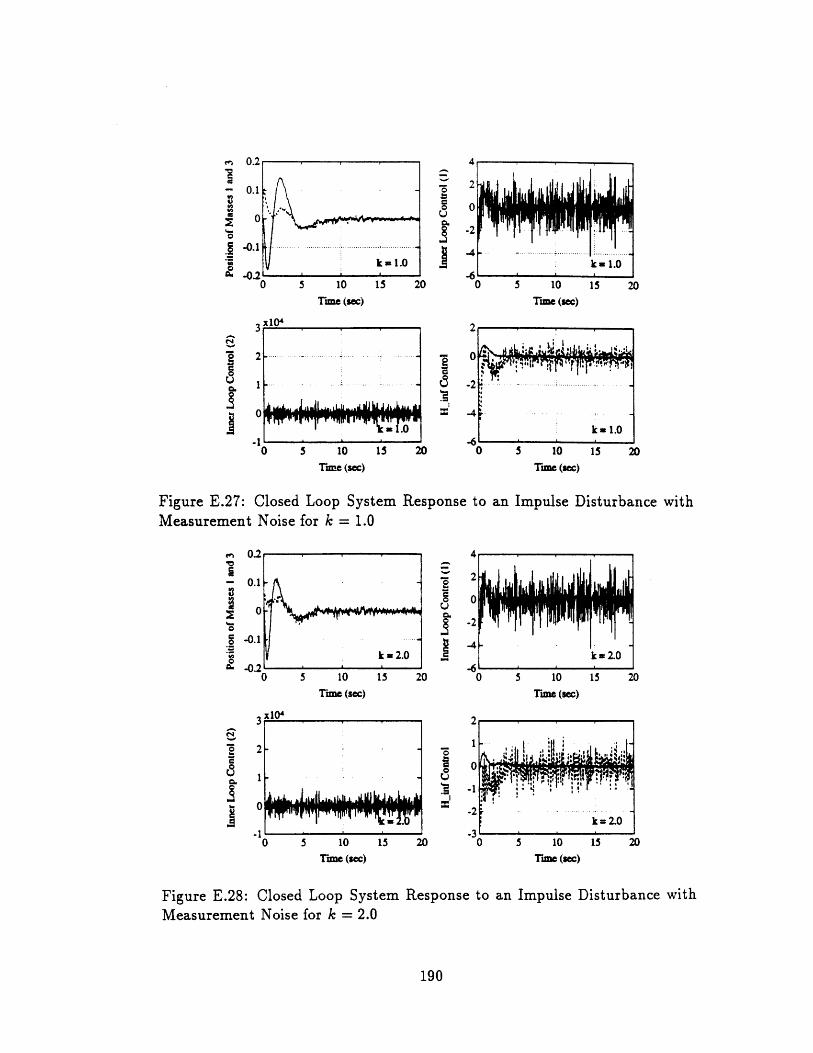
5 10Time (sec)

0 5 10Time (sec)

Figure E.27: Closed Loop SystMeasurement Noise for k = 1.0

0 5 10

Time (sec)

3

0 ~4*~M4W5 10

Time (Sec)

20 0

k

-2-4 .

k 1.015 20 0 5 10

Tunme (sec)

15 20 0 5 10Time (mc)

15 20

15 20

Response to an Impulse Disturbance with

2

0

-2

-4k=2.0

15 20 0 5 10

Time (sec)15 20

zu U 3 lU 13 lU

Time (sec)

Figure E.28: Closed Loop System Response toMeasurement Noise for k = 2.0

an Impulse Disturbance with

190

k a 1.0

''

-1

j0

3r

•A

0.2

-0.2a-_ r,

0.nj.I ¶ 2

0 10 20 30 40 0 10 20 30 40Time (src) Time (sec)

0 10 20 30 40Time (rsc)

Figure E.29: Closed Loop System Response to a Sinusoidal Disturbance fork = 0.5

. . . /o..

|S..0 20 30 4

10 20 30 4.21

0 0Time (Src)

10 20 30 40Time (sec)

10 20 30 40Tnme (sec)

Figure E.30: Closed Loop System Response to a Sinusoidal Disturbance fork = 1.0

191

.... .. 0*ki

-0.1

-02

.. . .........

" : " '- '•. .• . _ .4 0

1.0-\

·· _""I I

.-

AL

I I I ,

-··

g1

- II I I

A A

I o0

0.1

-0.1

.)2'0

11

10 20 30 40Time (sec)

10 20Time (sec)

30 40

10 20 30 40Tame (sec)

Figure E.31: Closed Loop System Responsek = 2.0


0 5 10 15

Time (sec)) 5 10 15 20

Tame (sec)

-40

0 5 10 15 20Tume (sec)

Figure E.32: Closed Loop System Response to a Reference Step Change fork = 0.5

192

- . .

i k i 2 II • k=2.. . . ,

k, 2.0

:'; :' ;",I

• . • ,

..............------..---.......

k = 0.5I I I

ii i I, I·--~.-.~-.-1.

k - .

.. ....... ........... -----------..

..... ... ·... ·. ·. ·.... .k 0.5

z I9I

_q

-I

A6&

jU

. = I

, I

J.L&I II

i.

l.n

0

'U

5 10 15 20 0 5 10 15 20Time (sec)

0 5 10 15 20Time (see)


5 10 15 20Time (sec)

0 5 10 15 20Time (sec)

0 5 10 15 20Time (sec)


193

k M= 1.0, I i I" " " " "

r?-"-----.~k--------1-- 0

' [ i .

Time (.rc)

k = 1.0

0.5

k =2.0 k = 2.0

........-.. ........ k.- 2.0...

k = 2.0

I

· ·

ZLu

•irll |

z""

"- - .A " ou0

'll

-M Ai

-M11W

tln

a method for robust control of systems with parametric

Documents