a method for the approximation of functions defined by ... · pdf filea method for the...

A Method for the Approximation of FunctionsDefined by Formal Series Expansions

in Orthogonal Polynomials*

By Jonas T. Holdeman, Jr.

Abstract. An algorithm is described for numerically evaluating functions defined

by formal (and possibly divergent) series as well as convergent series of orthogonal

functions which are, apart from a factor, orthogonal polynomials. When the

orthogonal functions are polynomials, the approximations are rational functions.

The algorithm is similar in some respects to the method of Padé approximants. A

rational approximation involving Tchebychev polynomials due to H. Maehley and

described by E. Kogbetliantz [1] is a special case of the algorithm. ■

1. Introduction. The solutions to many physical problems are obtained as

expansions in (infinite) series of orthogonal functions. When the series are con-

vergent they can in principle be approximated to any accuracy by truncating the

series at the proper point. When the series are weakly convergent or divergent, the

procedures for their numerical evaluation become rather ad hoc and a more general

approach would be useful. In the following sections we describe an approximation to

functions defined as infinite series of orthogonal functions which are (apart from a

factor) orthogonal polynomials. The approximation takes the form of the ratio of

two functions, the denominator function being a polynomial. When the orthogonal

functions are polynomials, the approximating function is rational.

The derivation of the algorithm will be formal and no real proofs are given.

Indication that the algorithm is at least sometimes valid is provided by the numer-

ical examples in Section 6. While the derivations could probably be made rigorous

in the case of absolutely convergent series, interesting cases occur with divergent

series such as the examples of Section 6. Numerous other practical applications of

the algorithm have been made in the past year at Los Alamos Scientific Laboratory.

The success of these examples would justify an effort at finding a class of functions

representable by divergent series for which the algorithm is applicable.

2. The Approximation. The approximations we shall discuss fall roughly into

two problems. The first of these is the approximation problem, that is, given a

function (or equivalently its expansion), find an easily calculated approximation to

the function. The second problem is the summation of infinite series, that is, given

an infinite series (which may not be convergent in the ordinary sense), assign a sum

to the series which gives the same value as the ordinary summation method when

the series is convergent. Clearly the two problems cannot be sharply separated. In

this paper however we will lean more toward the second problem.

For simplicity we assume the functions we will encounter are real on the real

Received December 14, 1967, revised August 5, 1968.* Work performed under the auspices of the U.S. Atomic Energy Commission.

275

License or copyright restrictions may apply to redistribution; see http://www.ams.org/journal-terms-of-use

276 JONAS T. HOLDEMAN, JR.

interval [a, b]. The generalization to complex functions on the real interval [a, b]

is trivial and the final results are identical to those which will be given.

The quantity to be evaluated is given in the form,

(1) /(*)-£«*!(*).

The basis functions {gi} are assumed to be orthogonal on [a, b] with weight function

o)(x) and normalization ßt and, apart from a factor, to be orthogonal polynomials,

(2) gn(x) = g0(x)qn(x) ,

where {</„} are orthogonal polynomials of exact degree n with weight function

go2«}.

We introduce a set of complementary polynomials {pi} orthogonal on [a, b] with

weight function co. The approximation to / is then given by

M J N M I N

(3) f(x) = ]£ amgm(x) / ^ bnpn(x) = g0(x) 22 a,mqm(x) / X) b„pn(x) ,

where the sets of coefficients {a,} and {bi} must satisfy

N M »

(4) f(x) ^2bnpn(x) - ^2amgm(x) = X) pmgm(x) .n=0 ro=0 m=- M+N+l

We take bo = 1 and call this the standard normalization. Other choices of normaliza-

tion of the coefficients may at times be more convenient. If we were to use the al-

gorithm to compute the inverse of / as a series of polynomials {p,}> then a0 = 1

might be the most appropriate normalization.

To solve the set of Eq. (4) it is convenient to introduce a matrix Hs associated

with the function / whose element H!mn is the coefficient of gm(x) in the expansion of

f(x)pn(x) in terms of the set {gt\. An integral representation of the elements H! is

given by

(5) Hin = Mm-1/ f(x)gm(x)pn(x)u(x)dx.J a

The first column of H1 is proportional to the expansion coefficients of f(x),

(6) Hio = poCm ,

and subsequent columns can be generated from the first by recursion. To see this

we note the following properties of {<7»j.

(i) Orthogonality.

(7) / gm(x)gn(x)w(x)dx = ßmSmn ,J a

where ôm„ = 1 if m = n and 5mn = 0 otherwise,

(ii) Closure.

OD lb

(8) f(y) = Hßn~lgn(y) j f(x)gn(x)u(x)dx .


A METHOD FOR THE APPROXIMATION OF FUNCTIONS 277

(iii) Linear Recursion.

(9) 9n+i(x) = (anx + ßn)gn(x) — yngn-i(x) ,

which remains valid for n = 0 when g-\(x) is replaced by 0. The complementary

polynomials {p¿} satisfy (7) and (8) with normalization hi and

(10) Pn+\(x) = (AnX + Bn)pn(x) — CnPn-\(x) ,

again valid for n = 0 when p~\(x) is replaced by zero.

Note that if we write

(11) Vn(x) = knx + kn'xn~l + • • • , po(x) = fco ,

then

/<n\ An = Kn+l/Kn , Un = An (/Cn_|_i//Cn_|_i Kn /Kn) ,

Cn — Anhn/ (An-lhn-l) = kn+ikn-\hn/ (fc„ ftn-l) ■

Similar relations hold for the ¡firm¡. From the recursion relations (9) and (10) for the

{¡7m} and the {pn) we see the elements of H! satisfy the recursion relation

(13) ~. \Hmn -\ Jl»+l,ri + Hm—l,n = ~7~ Hm,n+1 H T~ Hm¡n—1 •LA„ amJ «m+i am_i ^L„ /1„

Since this relation remains valid for m or n equal to zero provided we set H{n-\ =

HLitn = 0 in Eq. (13), any segment of the matrix can be generated by recursion from

the first column or from the expansion coefficients of /.

Finally for later use we note that the elements of the inverse of Hs are given by

(14) (H'yl = v.nhm-xHnT = hm~l f f-1(x)gn(x)pm(xMx)dx,J a

as can be seen by multiplication by (5) and use of the closure relations (8).

We now write the exact relation

(15) B(x)f(x) - A(x) = r(x) ,

where r(x) is a remainder and is related to the error in the approximation. Multiply-

ing Eq. (15) by ßm~lgm(x)w(x)dx and integrating over [a, b] yields the set of equations

N

(16) 2-f Hninbn ~ Cfm = pm ,ra=0

with

(17) r(x) = X) Pmgm(x) .

We now require pm to be zero for m á M + N. We note that such a requirement

is the basis of the Padé approximation to a power series. The equations to be solved

for the coefficients of A and B are

N

(18) 'EHLbn = -Hio = -fc0cm, M+l^mtSM + N,71 = 1

andN

(19) am = E Hinbn , 0 ^ m ^ M .



The coefficients of r(x) are given by

(20) pm=TlHinbn, M + N+l^m.

We define a "Padé-like" table as a two-dimensional array of elements, the

[N, M] element being the approximation with numerator of order M and de-

nominator of order (or degree) N. It can easily be shown (by expansion of the

determinants by minors) that the [N, M] approximation can be written as the ratio

of determinants

Y¿HÍogm(x)ro=0

HfAf+1.0

Y^Hingm(x) ••• Y^Hi,Ngm(x)m.= 0 m= 0

Hm+i,nHf-

M+l,n

Hi,

(21) [N,M](x) =M+N.O Hu,M+N,n HiM+N.N

po(x)

HfM+1,0

Pn(x)

HfM+l,n

Pn(x)

fM+l,N

Hf

Hm+N.O • - " Hii+N,n ' ■ ■ Hm+N,N

Note that this expression uses a nonstandard normalization. In a similar manner

the remainder r(x)/B(x) can formally be expressed as the ratio of the two deter-

minants above except that the sums over the index m in the numerator are over all

m such that m > M + N.

When M ¡î N, the approximation can be written in two forms. The first form is

the improper fraction,

(22)A (x) _ ^2^Zo amgm(x)

Bit) Zio &»?„(*) '

where the coefficients are given in Eq. (18) and (19) with M = N + L. The second

form is the polynomial plus proper fraction

(23)A(x)

B(x)

A(x)

B(x)= D(x) + ^( = Yjdigi(x) + .

ZJV-l _ / sm=0 amgm\X)

^n=obnPn(x)

The coefficients bn are obtained in both cases by solving Eq. (18) with M = N + L.

If we expand the quantity

(24) B(x)f(x) - B(x)D(x) - A(x) = r(x) ,

we find the coefficients ä~m are given by

(25)

¿V L

am / , tímnOn / . tlmlQjl ,n—0 1=0

and the coefficients di are given by solving

0 Ú m ^ N - 1 ,



(26) T,H*ldl=T,Hinbn, N^m^N + L.1=0 71=0

As the notation indicates, HB is the matrix associated with the polynomial B(x).

The Eqs. (26) are easily solved due to the simple structure of HB. (The submatrix in-

volved in Eq. (26) is triangular.)

The coefficients for the two forms (22) and (23) are related by

(27) ^L ~ aN+LfäN+L-L '

dh-

and

l — atf+L-l — ¿_i dl,-mHN+L-l,L-m I Hn+L-1,L-1 > 1 = I = L ,L ,7t=0 J /

(28) U- = am - J^HZ.l-i dL-i, 0 á m ^ N - 1 .1=0

These latter equations contain no direct reference to /, and indeed they provide a

way of calculating the proper fraction plus finite sum from any improper fraction.

If the fraction is rational, they provide a method for applying the Euclidian al-

gorithm to find common factors without first transforming the (finite) series of

orthogonal polynomials to a power series.

3. Relation to a Least Squares Approximation. One measure of the weighted

error of the rational approximation to the function f(x) on the interval [a, b] is the

quantity

(29) e= I [B*(x)f(x) - A*(x)]2œ(x)dx.J a

(If the functions were complex, the squared quantity would be replaced by the

squared magnitude.) This error is a function of the coefficients {a¿*} and {b*}. For

the moment consider B*(x) to be determined and A*(x) to be a polynomial of de-

gree M. Then e is a quadratic function of the coefficients ¡o,*}. This error is min-

imized when for each fc ^ M,

— = -2 / [B*(x)f(x) - A*(x)]gk(x)œ(x)dx = 0 ,dak* J"

or

N

(30) ak* = ^HLbn*, O^k^M .71=0

Thus the set {ak*\ which minimizes the error e is just that set given by the algorithm

once the set {&»*} is determined.

Now consider the minimization e with respect to the set of coefficients {b*}.

For each k ;£ N,

de= 2 / [B*(x)f(x) - A*(x)]f(x)pk(x)w(x)dx = 0 ,

or



(31) ¿ E Hflnb* - ai* Lh'u = 0 , 0 ^ fc á A ,i=o Ltí=o J

where a* = 0 for l > M.

This set of equations is to be solved for the bk*'s consistently with the set of

equations (30) and a subsidiary condition involving the normalization for the

ak*'s to give the least squares approximation to f(x). Although in principle the co-

efficients can be obtained from Hs, in practice this is not always possible so the

coefficients in Eq. (31) cannot be regarded as known.

To obtain the equations of the algorithm, we hold M fixed and let N —> ». The

set of Eqs. (31) becomes

(32) £ £ HÍK* \ßiHflk = ¿ al*ßtf\k, 0 g fc < °o .1=0 Ln=0 J i=0

Now we can multiply by the inverse of H! (14) and obtain,

¿i/U„* = a?, 0£l£M,(33) "=°

¿i/U„*=0, M+1^1.71=0

If we now truncate the set of Eqs. (33) we arrive at the equations of the al-

gorithm. It is then clear that the algorithm does not yield a least squares approxi-

mation except possibly in the limit N —> <=o.

4. Some Remarks on Convergence. In this section we will examine the con-

vergence of the first two rows of the Padé-like table under suitable restrictions on /.

We note that the limit

(34) lim \-±- + ^±i - £=]

is finite. This condition is satisfied by all of the classical orthogonal polynomials. We

restrict /, defined by

OO

(35) f(x) = X cmgm(x) ,777=0

to be such that

(36) cm ~ Nm .

We recall the following transformation for improving the convergence of the

series (35). By formally rearranging the series and using the recursion relation for

{<7¿} we can write

00

(37) f = (x — a)-1 X) cm'gm(x) ,771=0

where

(38)_ Ctti-1 , Tm+lCm+l _ ß_m .

T" a \cm .«TTi-i «TTi+i Lam J



If a is chosen such that

(39) lim -— + 3^ - &=1 = a ,771—.30 L«771—1 «771+1 «77lJ

then

(40) c¿ ~ N'm'-1,

and the series (37) is (asymptotically) more rapidly convergent. We shall return to

this result shortly.

We note that the elements [0, M] of the first row of the Padé-like table are

simply the truncated sums

M M

(41) {0,M](x) = J^amgm(x) = J^cmgm(x).771=0 771=0

If the sum (35) is convergent to /, then the sequence of elements of the first row of

the table are convergent to /.

Now consider the elements of the second row of the table. Notice that

(42)

7, it] a \Bo ßiu+i , Jm+2 Cm+2 . 1 CmtlM+l,\/tlM+l,0 — A-0 ~T~ ~~ +-1"

L^0 «Af+1 «M+2 Cm+1 CXm Cm+iJ

~ Ao If2 + -~ + ^ - ëM±k\ + ear1)LAo am «AÍ+2 «Af+lJÏA/+2

For large M, we use (12) and (13) to write B(x) in a form which displays the posi-

tion of the pole in the approximation,

(43) B, (x) ~ -k\— + ^m - §J1 - x~\,LöAi-l OCM+l CUM J

where K depends on the normalization. As M —>• », the pole moves to a position

identical to that in Eqs. (37) and (39).

The numerator AM(x) is given by

M

(44) AM(x) = X amgm(x) ,777 = 0

where for large M,

(AZ.\ _ je! Cm~x _|_ Tm+lCm+l _ \ §m_1_JM+2 , /?M+2

lam_l «771+1 L«m <XM a.M+2 «Ai+lJ

In the limit M —* «>, (with K = 1) this is identical to (38) and (39) and in this limit

the approximation [1, M] is identical to the transformation mentioned at the be-

ginning of this section. It is tempting to conjecture that as one moves down the

table, the row-wise convergence improves. Numerical evidence indicates that this is

the case, but proof remains to be found.

We conclude this section with a formula for the remainder RNM(x),

(46) RnM(x) = f(x) - AM(x)/BN(x) ,

when {g,} = {Pn'-'x-ß)(x)}, the set of Jacobi polynomials. Referring to Szegö [3, Eqs.

(4.62.19) and (9.2.1)], we find



E lhnia'ß)r1Pn(a-ß\x)Qnl"-ß)(y)n=N+l

(47)

-a-ßY(N + 2)Y(N+a + ß + 2)

(2N+ « + ß + 2)r(A + « + l)r(A + ß + 1)

»fof (»)Q*r("'%) - Py("w(s)Qfo?(y)]£ - 2/ J'

The expansion coefficients of BnRnm are zero when their index is less than M -\- N

and equal to those of BNf otherwise. It then follows that

RnM(x) =

(48)

Y(N + M + «)r(A + M + « + /3 + 2)21~"-V'm

(2AT + 2M + a + /3 + 2)T(A + « + l)r(A + /3 + 2)£¿Kz)

v 1 Á \PNJM+Áx)Q^M(y) - PfoStoQ&ß+i Û/)"L, ,.X2«%L *-« r«'y

where eiirao>(y) = (y — l)a(y + l)ß and C is an ellipse with foci at =1=1 and enclosing

no singularity of/. With special values for « and ß, (48) gives representations for the

remainder in approximations involving Gegenbauer, Legendre, and Tchebychev

polynomials.

5. Numerical Examples. We now consider the application of the algorithm to a

particular case, though some of the remarks made later are based on experience with

other functions. Consider the function

(l - ¡A-1-*» f, (l+in)i p(49) -*\hr) =li(2l + l)^~^iPl(x)>

where {¡7,} = {Pi}, the set of Legendre polynomials. The symbol (a) ¡ in JSq. (49) is

defined by

(50) (o)o=l, (a)i = a(a+l) ■■■ (a + l- 1) .

In particular we consider Eq. (49) with ij = 1.

The function in Eq. (49) when multiplied by the proper factor is the Coulomb

scattering amplitude which one obtains in the nonrelativistic scattering of charged

particles. The coefficients of the Legendre polynomials behave asymptotically

as Z1"1"2"1 as I —> oo. The series is divergent, but nevertheless represents the function

on the left [4].

Referring to the Padé-like table, we will consider the three-diagonal approxi-

mations [4, 4], [8, 8], and [12, 12]. These three approximations were calculated on

a LASL-Control Data 6600 computer. Single-precision floating point numbers are

represented on this machine by a 48 bit mantissa (about 14 decimal digits). In Fig. 1

we have plotted the magnitude of the relative error. From Fig. 1 (and other calcula-

tions) several things are immediately apparent. As we move down the diagonal of

the Padé-like table (or more generally as M + N increases), the relative error is

reduced over the interval [ — 1, 1). In these numerical calculations, the minimum

error is of course bounded by the accuracy of the representation of the number (in

this case ~10-14). Since this function has a branch point at x = 1, and sufficiently

close to the branch point no finite configuration of poles and zeroes can "mock up"



the branch point, the approximation fails close to a; = 1.

10°

IQ"2

I0"4

wO

w01

| io-6o07k_

^~

o

S I O"8'EenoE

IO"10

IO"12

-1.0 -0.6 -0.2 0.2 0.6 1.0

x

FlGUKE 1

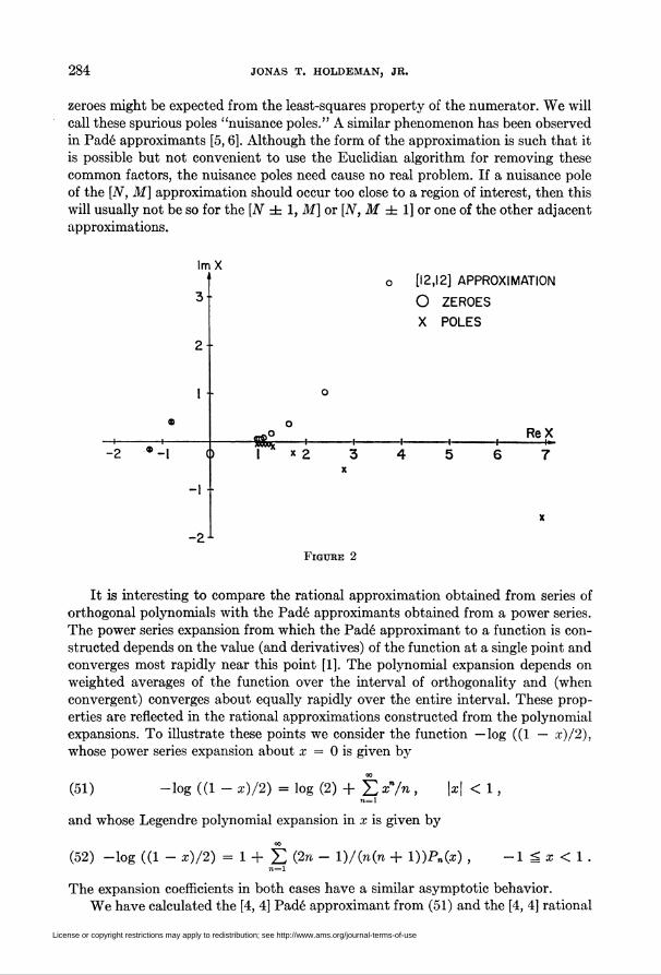
If we calculate the positions of the poles and zeroes in the complex plane for

various finite approximations we find that they tend to He along the branch cut from

x = 1 to infinity and tend to accumulate at x = 1. We show this behavior in Fig. 2,

where we have plotted their positions for the [12, 12] approximation. If in Eq. (49)

we allow 17 to vary, we find that as 17 —> 0, the poles and zeroes near the cut move

closer to the real axis. Off the real axis the error in the approximation is somewhat

larger than that indicated in Fig. 1. To the left of x = 1 and along the lines with

the imaginary part of x equal to ±1/2, the magnitude of the relative error is about

10-8 and IO-9 for the [8, 8] and [12, 12] approximations and about 10~4 for the [4, 4]

approximation. Thus the rational approximation is a useful analytic continuation

into the complex plane.

In practice it is found that in addition to poles along the branch cut of the

function of Eq. (49), poles appear elsewhere in the complex plane in positions not

related to the analytic structure of the approximated function. The positions of

these poles vary rapidly from an approximation of one order to the next, and (if

allowed by the order of M) they are usually cancelled by zeroes of the numerator

(the numerator and denominator possess common factors). This cancelling by the



zeroes might be expected from the least-squares property of the numerator. We will

call these spurious poles "nuisance poles." A similar phenomenon has been observed

in Padé approximants [5,6]. Although the form of the approximation is such that it

is possible but not convenient to use the Euclidian algorithm for removing these

common factors, the nuisance poles need cause no real problem. If a nuisance pole

of the [N, M] approximation should occur too close to a region of interest, then this

will usually not be so for the [N ± 1, M] or [N, M =b 1] or one of the other adjacent

approximations.

ImX

3

2 ■

-2

-I

-2

[12,12] APPROXIMATION

O ZEROES

X POLES

ReX

x 2

Figure 2

It is interesting to compare the rational approximation obtained from series of

orthogonal polynomials with the Padé approximants obtained from a power series.

The power series expansion from which the Padé approximant to a function is con-

structed depends on the value (and derivatives) of the function at a single point and

converges most rapidly near this point [1]. The polynomial expansion depends on

weighted averages of the function over the interval of orthogonality and (when

convergent) converges about equally rapidly over the entire interval. These prop-

erties are reflected in the rational approximations constructed from the polynomial

expansions. To illustrate these points we consider the function —log ((1 — x)/2),

whose power series expansion about x = 0 is given by

(51) -log ((1 - x)/2) = log (2) + £ xn/n , \x\ < 1,<i—i

and whose Legendre polynomial expansion in x is given by

(52) -log ((1 - x)/2) = 1 + ¿ (2n - l)/(n(n + l))P„(a;) , -lgKl.71=1

The expansion coefficients in both cases have a similar asymptotic behavior.

We have calculated the [4, 4] Padé approximant from (51) and the [4, 4] rational



polynomial approximant from (52). In Fig. 3 we compare the magnitudes of the

relative errors. As previously mentioned, we see that the [4, 4] Padé approximant

has a very small error near x = 0 with the error rising slowly away from x = 0. By

contrast, the [4, 4] rational polynomial approximation fits the function with about

the same (average) accuracy over the interval ( — 1, 1) with eight zeroes of the

(relative) error function lying in the interval ( — 1, 1).

o

>

o

CD■o

"ECPo£

One more point should be made. If the expansion (52) is truncated at n = 8,

rearranged in powers of x, and the [4, 4] Padé approximant constructed from this

truncated series, the result must be identical to the [4, 4] rational polynomial

approximation from the uniqueness of the rational form.** The coefficients from

which the Padé approximants are constructed are a function of the truncation point

and it is not often that the infinite series (52) can be rearranged into a power series

(51).We will now consider in detail two other closely related examples. These ex-

amples are limiting cases of the expansion of (1 — x)a as « —» — 1 [4]. In the previous

example the indications (admittedly based on scanty evidence) were that the

diagonal sequence of approximations was converging. It may happen that no

diagonal sequence of approximations exists.

Consider first the rational approximations to the function expanded in a (diver-

gent) series of Legendre polynomials {P¿¡,

(53) (x - I)"1 = £ (21 + 1)^(2Z + l)Pi(x) ,

where \p is the logarithmic derivative of the gamma function. For our purposes it is

sufficient to know that \p satisfies the recursion relation

I wish to thank G. A. Baker, Jr. for a discussion on this point.



(54) Hl + i) = Hl) + i/l ■

It can be shown by induction using the recursion relations (14) and by the symmetry

of W that

,r^\ Hin = (2m + 1)H™- + 1) , m ^ n ,

= (2m + l)Hn + 1) , m-^n.

Referring then to the determinantal form (21) of the rational approximation

it is easily seen that

M

(i) [0, M](x) = £ (2m + l)Hm + l)Pm(x) ,

(56)

771=0

(ii) [l,M](x) = l/(x-l), 0^1,

(iii) [N,0](x) = l/(s-l), 1ZN,

(iv) [N, M](x) is indeterminant for M > 0 and A > 1

Since the original series was divergent, the sequence of elements in the first row is

not convergent. The elements of the second row and those of the first column are

(obviously) convergent to the function (x — l)-1, and no other row or column nor

any diagonal sequence even exists.

A similar result obtains for the generalized function

(57) 5(1 - x) = £ (I + l/2)Pi(x) ,1—0

where the {Pi} are again Legendre polynomials and 5 is the Dirac delta function.

The elements of the related matrix Hf are given by

(58) Hin = (m + 1/2) .

The elements of the Padé-like table are then given by

M

[0, M](x) = £ (m + h)Pm(x) , 0 g M ,771=0

(59) [l,M](x) = 0/(x-l), 0^M,

¡N,0](x)=0/(x-l), lg A,

[N, M](x) is indeterminant for M > 0 and N > 1 .

The remarks after the previous example are applicable also in this case.

6. Conclusion. Many additional properties of the approximation can be derived

for particular choices of the set {gi}. These properties may depend on special prop-

erties of the set under consideration and so are not generalizable to other sets of

orthogonal functions. These special properties may be very important in any given

problem.

As an example, suppose the interval of orthogonality is even, [ — a, a] and the

functions gn(x) and pn(x) are even or odd according as the index n is even or odd.

Then if a function is defined by an even (odd) series and an odd-odd (even-even)



approximation is attempted, the Eqs. (18) have no solution. Also the even-odd or

odd-even approximations are equal to adjacent nonvanishing elements in the table.

These remarks may be verified by referring to the determinantal form of the ap-

proximation (21) and noting that alternate elements of Hf vanish. In these even or

odd cases, some computing economy can be effected by rewriting the recursion re-

lation (12) for Hs so that it relates the elements Hfm,„, Hi±2¡n, Hi¡n±2, and reformulat-

ing the algorithm so that only the even (odd) elements of {g(} are involved (we take

B(x) to have only even terms in either case).

This work was performed during the author's tenure of a postdoctoral appoint-

ment at Los Alamos Scientific Laboratory, Los Alamos, New Mexico. In conclusion

the author would like to thank Dr. Charles Critchfield and members of group T-9

for extending to him the laboratory's hospitality and Drs. Leon Heller, John

Gammel, and especially William Beyer for many helpful discussions and suggestions

regarding the material presented here.

Michigan State University

Physics Department

East Lansing, Michigan 48823

1. E. G. Kogbetliantz, "Generation of elementary functions," in Mathematical Methods forDigital Computers, Wiley, New York, 1960. MR 22 #8681.

2. A. Erdélyi, et al., Higher Transcendental Functions, Vol. II, McGraw-Hill, New York,1953. MR 15, 419.

3. G. Szegö, Orthogonal Polynomials, Amer. Math. Soc. Colloq. Publ., Vol. 23, Amer. Math.Soc, Providence, R. I., 1959. MR 1, 14.

4. J. Holdeman, "Legendre polynomial expansions of hypergeometric functions with applica-tions." (To appear.)

5. G. A. Baker, Jr., J. L. Gammel & J. G. Wills, "An investigation of the applicabilityof the Padé approximant method," J. Math. Anal. Appl., v. 2, 1961, pp. 405-418. MR 23 #B3125.

6. G. A. Baker, Jr., "The theory and application of the Padé approximant method," inAdvances in Theoretical Physics, Vol. I, Academic Press, New York, 1965, pp. 1-58. MR 32 #5253.


a method for the approximation of functions defined by ... · pdf filea method for the...

Documents