a method to predict and understand fish survival … · a method to predict and understand fish...

A METHOD TO PREDICT AND UNDERSTAND FISH SURVIVAL UNDER DYNAMICCHEMICAL STRESS USING STANDARD ECOTOXICITY DATA

ROMAN ASHAUER,*yz PERNILLE THORBEK,x JACQUI S. WARINTON,x JAMES R. WHEELER,x and STEVE MAUNDkyEnvironment Department, University of York, York, United Kingdom,

zEawag, Swiss Federal Institute of Aquatic Science and Technology, Dübendorf, SwitzerlandxSyngenta, Environmental Safety, Berkshire, United Kingdom,

kSyngenta Crop Protection AG, Basel, Switzerland

(Submitted 12 September 2012; Returned for Revision 5 November 2012; Accepted 30 November 2012)

Abstract—The authors present a method to predict fish survival under exposure to fluctuating concentrations and repeated pulses of achemical stressor. The method is based on toxicokinetic-toxicodynamic modeling using the general unified threshold model of survival(GUTS) and calibrated using raw data from standardfish acute toxicity tests. Themodel was validated by predicting fry survival in a fish earlylife stage test. Application of the model was demonstrated by using Forum for Co-ordination of Pesticide FateModels and Their Use surfacewater (FOCUS-SW) exposure patterns as model input and predicting the survival of fish over 485 d. Exposure patterns were also multipliedby factors of five and 10 to achieve higher exposure concentrations for fish survival predictions. Furthermore, the authors quantified how farthe exposure profiles were below the onset of mortality by finding the corresponding exposure multiplication factor for each scenario. Theauthors calculated organism recovery times as additional characteristic of toxicity as well as number of peaks, interval length between peaks,and mean duration as additional characteristics of the exposure pattern. The authors also calculated which of the exposure patterns had thesmallest and largest inherent potential toxicity. Sensitivity of the model to parameter changes depends on the exposure pattern and differsbetween GUTS individual tolerance and GUTS stochastic death. Possible uses of the additional information gained frommodeling to informrisk assessment are discussed. Environ. Toxicol. Chem. 2013;32:954–965. # 2013 SETAC

Keywords—Dose-response model Time-variable exposure Aquatic toxicity Pesticide fate model Carry-over toxicity

INTRODUCTION

Assessing the ecological risk of plant protection products(PPPs) requires the comparison of toxicity data for sensitivenontarget species with worst-case predicted exposure concen-trations in the environment. Toxicity data used in theseassessments usually are obtained from studies in which exposureconcentrations are maintained for the duration of the experi-ments, usually lasting several days (for acute studies) to severalweeks (for chronic studies). However, under realistic environ-mental conditions, concentrations of PPPs in aquatic systemswill fluctuate, and exposure profiles may vary substantially [1–3]. Risk assessments do not typically consider the nature ofeffects on nontarget species from fluctuating exposures that arelikely to be encountered in the field; instead, peak or time-weighted average concentrations usually are used [4–6]. Toassess the environmental risk of PPPs, time series concentrationsin surface water bodies are predicted using environmental fatemodels [3,7]. At present, it remains unclear how to appropriatelyintegrate these exposure profiles with the effect assessments torefine the risk assessments [3].

Classical data analysis methods, more specifically concen-tration–effect curve models do not account for temporal aspectsof exposure and toxicity [5,8–11]. However, in recent yearsalternative toxicity models that consider temporal aspectsof toxicity have been developed [3,9,12]. Toxicokinetic-toxicodynamic (TKTD) models simulate the time course ofprocesses that lead to intoxication and can account for carry-over

toxicity and delayed effects, which can be caused by slowelimination, slow organism recovery, or a combination of bothprocesses [13]. Moreover, they can process fluctuating or pulsedexposure concentrations as an input to predict survival over time.Thus, they are well-suited for risk assessment of dynamicchemical stress [3,9]. Recently, TKTD models for survival havebeen unified and integrated in the general unified thresholdmodel of survival (GUTS) [8].

Standard toxicity tests are typically carried out withmaintained exposures, whereas measured and simulatedexposure to PPPs in water bodies generally occur in fluctuatingand highly variable patterns [1–4,7]. Thus, toxicity must beextrapolated from relatively constant to relatively variableexposure profiles. Toxicokinetic-toxicodynamic models simu-late the time course of processes leading to toxicity, includingprocesses that cause carry-over toxicity or delayed ef-fects [9,13]. Carry-over toxicity can be caused by bioaccumu-lation and slow elimination, as well as slow toxicodynamic(TD) organism recovery [8,13]. The ability to model carry-overtoxicity is the key reason why greater confidence can be placedin toxicity extrapolations for fluctuating or pulsed exposurepatterns based on TKTD models rather than on predictionsbased on time-weighted averages [8,9,13,14]. Furthermore,TKTD model parameters have a mechanistic interpretation andcan thus be evaluated with other studies, such as bioaccumu-lation tests. Toxicokinetic (TK)models have been demonstratedto accurately predict internal concentrations in fish [15]. Severalreviews of the extrapolation of toxicity to fluctuating exposuresare available [5,9,16,17], and some studies have investigatedthe calibration and predictive power of TKTD models forsurvival [14,18,19]. Thus, TKTD models offer options forhigher-tier risk assessment tools that can be usedfor robust evaluations of likely effects resulting from time-

All Supplemental Data may be found in the online version of this article.� To whom correspondence may be addressed

([email protected])Published online 30 January 2013 in Wiley Online Library

(wileyonlinelibrary.com).

Environmental Toxicology and Chemistry, Vol. 32, No. 4, pp. 954–965, 2013# 2013 SETAC

Printed in the USADOI: 10.1002/etc.2144

954

varying exposure, which is likely to be the rule rather than theexception.

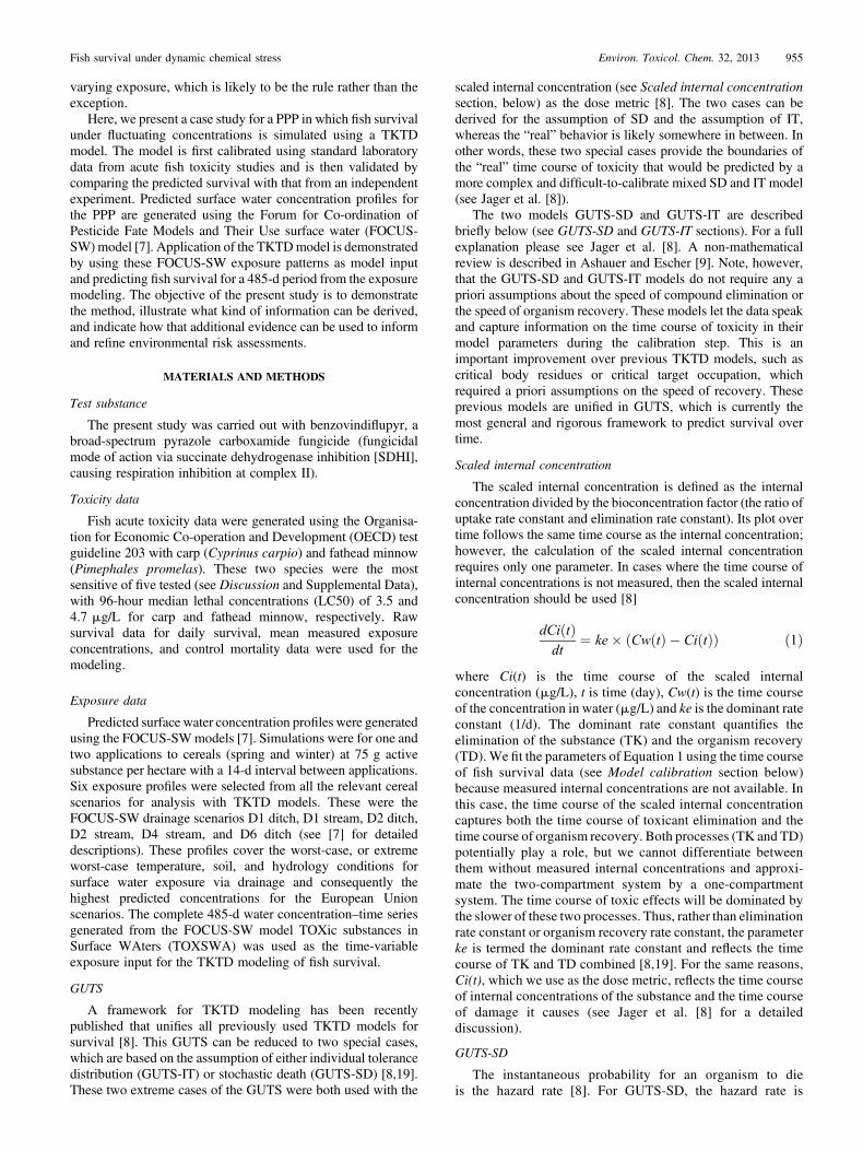
Here, we present a case study for a PPP in which fish survivalunder fluctuating concentrations is simulated using a TKTDmodel. The model is first calibrated using standard laboratorydata from acute fish toxicity studies and is then validated bycomparing the predicted survival with that from an independentexperiment. Predicted surface water concentration profiles forthe PPP are generated using the Forum for Co-ordination ofPesticide Fate Models and Their Use surface water (FOCUS-SW)model [7]. Application of the TKTDmodel is demonstratedby using these FOCUS-SW exposure patterns as model inputand predicting fish survival for a 485-d period from the exposuremodeling. The objective of the present study is to demonstratethe method, illustrate what kind of information can be derived,and indicate how that additional evidence can be used to informand refine environmental risk assessments.

MATERIALS AND METHODS

Test substance

The present study was carried out with benzovindiflupyr, abroad-spectrum pyrazole carboxamide fungicide (fungicidalmode of action via succinate dehydrogenase inhibition [SDHI],causing respiration inhibition at complex II).

Toxicity data

Fish acute toxicity data were generated using the Organisa-tion for Economic Co-operation and Development (OECD) testguideline 203 with carp (Cyprinus carpio) and fathead minnow(Pimephales promelas). These two species were the mostsensitive of five tested (see Discussion and Supplemental Data),with 96-hour median lethal concentrations (LC50) of 3.5 and4.7 mg/L for carp and fathead minnow, respectively. Rawsurvival data for daily survival, mean measured exposureconcentrations, and control mortality data were used for themodeling.

Exposure data

Predicted surface water concentration profiles were generatedusing the FOCUS-SWmodels [7]. Simulations were for one andtwo applications to cereals (spring and winter) at 75 g activesubstance per hectare with a 14-d interval between applications.Six exposure profiles were selected from all the relevant cerealscenarios for analysis with TKTD models. These were theFOCUS-SW drainage scenarios D1 ditch, D1 stream, D2 ditch,D2 stream, D4 stream, and D6 ditch (see [7] for detaileddescriptions). These profiles cover the worst-case, or extremeworst-case temperature, soil, and hydrology conditions forsurface water exposure via drainage and consequently thehighest predicted concentrations for the European Unionscenarios. The complete 485-d water concentration–time seriesgenerated from the FOCUS-SW model TOXic substances inSurface WAters (TOXSWA) was used as the time-variableexposure input for the TKTD modeling of fish survival.

GUTS

A framework for TKTD modeling has been recentlypublished that unifies all previously used TKTD models forsurvival [8]. This GUTS can be reduced to two special cases,which are based on the assumption of either individual tolerancedistribution (GUTS-IT) or stochastic death (GUTS-SD) [8,19].These two extreme cases of the GUTS were both used with the

scaled internal concentration (see Scaled internal concentrationsection, below) as the dose metric [8]. The two cases can bederived for the assumption of SD and the assumption of IT,whereas the “real” behavior is likely somewhere in between. Inother words, these two special cases provide the boundaries ofthe “real” time course of toxicity that would be predicted by amore complex and difficult-to-calibrate mixed SD and IT model(see Jager et al. [8]).

The two models GUTS-SD and GUTS-IT are describedbriefly below (see GUTS-SD and GUTS-IT sections). For a fullexplanation please see Jager et al. [8]. A non-mathematicalreview is described in Ashauer and Escher [9]. Note, however,that the GUTS-SD and GUTS-IT models do not require any apriori assumptions about the speed of compound elimination orthe speed of organism recovery. These models let the data speakand capture information on the time course of toxicity in theirmodel parameters during the calibration step. This is animportant improvement over previous TKTD models, such ascritical body residues or critical target occupation, whichrequired a priori assumptions on the speed of recovery. Theseprevious models are unified in GUTS, which is currently themost general and rigorous framework to predict survival overtime.

Scaled internal concentration

The scaled internal concentration is defined as the internalconcentration divided by the bioconcentration factor (the ratio ofuptake rate constant and elimination rate constant). Its plot overtime follows the same time course as the internal concentration;however, the calculation of the scaled internal concentrationrequires only one parameter. In cases where the time course ofinternal concentrations is not measured, then the scaled internalconcentration should be used [8]

dCiðtÞdt

¼ ke� CwðtÞ � CiðtÞð Þ ð1Þ

where Ci(t) is the time course of the scaled internalconcentration (mg/L), t is time (day), Cw(t) is the time courseof the concentration in water (mg/L) and ke is the dominant rateconstant (1/d). The dominant rate constant quantifies theelimination of the substance (TK) and the organism recovery(TD). We fit the parameters of Equation 1 using the time courseof fish survival data (see Model calibration section below)because measured internal concentrations are not available. Inthis case, the time course of the scaled internal concentrationcaptures both the time course of toxicant elimination and thetime course of organism recovery. Both processes (TK and TD)potentially play a role, but we cannot differentiate betweenthem without measured internal concentrations and approxi-mate the two-compartment system by a one-compartmentsystem. The time course of toxic effects will be dominated bythe slower of these two processes. Thus, rather than eliminationrate constant or organism recovery rate constant, the parameterke is termed the dominant rate constant and reflects the timecourse of TK and TD combined [8,19]. For the same reasons,Ci(t), which we use as the dose metric, reflects the time courseof internal concentrations of the substance and the time courseof damage it causes (see Jager et al. [8] for a detaileddiscussion).

GUTS-SD

The instantaneous probability for an organism to dieis the hazard rate [8]. For GUTS-SD, the hazard rate is

Fish survival under dynamic chemical stress Environ. Toxicol. Chem. 32, 2013 955

calculated as

dHðtÞdt

¼ kk �max CiðtÞ � z; 0ð Þ þ h_controls ð2Þ

where dH(t)/dt is the hazard rate (1/d), kk is the killing rateconstant (L/[mg � d]), Ci(t) is the time course of the scaledinternal concentration (mg/L), t is time (day), z is the threshold(mg/L) and h_controls is the background hazard rate (controlmortality rate, 1/d). The GUTS-SD assumes that all individualsin the test population have the same threshold, z (see also Jageret al. [8] and Nyman et al. [19]). The survival probability—thatis, the probability of an individual to survive until time t—isgiven by

SðtÞ ¼ e�HðtÞ ð3Þwhere S(t) is the survival probability (�).

GUTS-IT

The GUTS-ITmodel assumes that the value of the threshold zdiffers among individuals in the test population and follows adistribution (see also Jager et al. [8] and Nyman et al. [19]).When the threshold is exceeded, it is assumed that the individualdies immediately. Here, GUTS-IT also uses the scaled internalconcentration as dose metric (Eq. 1) and the threshold z is thescaled internal concentration above which the individual diesinstantly. Thus, the number of deaths over time can be calculatedbased on the distribution of the threshold z in the population. Thecumulative log-logistic distribution of the threshold z iscalculated as

FðtÞ ¼ 1

1þ max0<s<t CiðsÞa

� ��b ð4Þ

where F(t) is the cumulative log-logistic distribution of thethreshold z over time (�), Ci(s) is the time course of thescaled internal concentration (mg/L), t is time (day), s (day) istime before the current point in time t, a is the median of thedistribution of z (mg/L), and b is the shape parameter ofthe distribution of z (�). The survival probability—that is,the probability that an individual will survive until time t—isgiven by

SðtÞ ¼ 1� FðtÞð Þ � e�h_controls�t ð5Þwhere S(t) is the survival probability (�) and h_controls is thebackground hazard rate (control mortality rate, 1/d).

GUTS-SD and GUTS-IT in multiple pulse exposures

Due to their inherent assumptions, the models GUTS-SD andGUTS-IT result in different survival predictions for repeatedpulse exposures. The SD approach assumes that death is a chanceprocess; thus, the proportion of a population that is killed by aseries of identical pulses remains constant, irrespective ofprevious exposure. The IT approach assumes that there is adistribution of tolerances in the exposed population so thattolerant individuals will not be affected by repeated exposure tothe same (or lower) toxicant concentrations. To illustrate theseassumptions, consider a hypothetical example with two identicalpulses in sequence, where the first pulse kills 50 out of 100 fish.Given that the interval between the two pulses is long enough forcomplete elimination of the substance and organism recovery,

GUTS-SD would predict that the second pulse kills 25 fish,whereas GUTS-IT would predict that the second pulse kills zerofish. Mortality is a chance process in GUTS-SD, with all fish inthe population having equal probabilities to die and the sameprobability applies at the first and second pulse. Mortality is adeterministic process in GUTS-IT, following a distribution ofthresholds in the fish population, where the first pulse kills themore sensitive fraction of all fish and the strong individualssurvive both the first and the second pulses. Thus, it is importantto use both models together (for detailed discussionssee [8,20,21]).

Model calibration

Raw data from the carp and fathead minnow toxicity testswere used in the model calibration. Mean measured concen-trations served as model input, whereas survival data for eachday and control mortality data served as calibration data. Inaddition to the toxicity studies, a fish bioconcentration (OECDtest guideline 305) test with bluegill sunfish (Lepomis macro-chirus) was available. The depuration rate constant (kd¼ 1.2802 1/d) from the bioconcentration study was used asinitial value for ke in the model calibration for carp, which wasthe first species for which we calibrated the TKTD model.

The parameters for GUTS-SD and GUTS-IT were found bymaximizing the log likelihood function (see Jager et al. [8] forderivation)

lnlðujyÞ ¼Xnþ1

i¼1

yi�1 � yið Þln Si�1 uð Þ � Si uð Þð Þ ð6Þ

where l is the likelihood, y is the time series of the number ofsurvivors, i is sampling date, n is the number of sampling dates, uis the vector of model parameters and S(u) is the survivalprobability given u. The likelihood was calculated for eachtreatment (test concentration in the acute toxicity test) and the lnlikelihoods for all treatments were summed. We then used thedownhill simplex algorithm to find the minimum -ln likelihood inparameter space. The parameter values at the smallest -lnlikelihood are the best fit parameter values and are used to predictsurvival in other exposure scenarios. Thus, information about thetime course of toxicity is extracted from the acute toxicity testdata, captured by the model and its parameter values, and thenused to predict survival with other concentration time series asinput (e.g., FOCUS-SW scenarios).

The parameters ke, kk, and zwere calibrated for the GUTS-SDmodel, and the parameters ke, a, and b were calibrated for theGUTS-IT model. The confidence limits were calculated byprofiling the likelihood [22] for each parameter separately. The95% confidence limits are reported. The mortality in the controlgroups was used to calibrate the background hazard rate (i.e.,approximate background mortality). Both the control andsolvent control survival data were combined for that analysis.The resulting control mortality rate h_controls was 0.018 (1/d)with confidence limits (0.001, 0.032) for carp. The survival datafor control fish in the acute toxicity test with fathead minnow didnot show any mortality. Because a background mortality rate ofzero is biologically impossible and causes computationalproblems during calibration, the control mortality rate h_con-trols was set to 0.00315 (1/d) for this species. This controlmortality rate corresponds to 10% survival over two years (730d), reflecting the natural life span of the fathead minnow. Thecontrol mortality rate was kept fixed when calibrating the othermodel parameters.

956 Environ. Toxicol. Chem. 32, 2013 R. Ashauer et al.

Model testing (validation)

A fish early life stage study (ELS; OECD test guideline210 [23]) with fathead minnow was available to independentlytest the model predictions with data other than the acute toxicitytest results. Survival of fry in the ELS study was compared tosurvival predicted with GUTS-SD and GUTS-IT. In the ELSstudy, testing was initiated with freshly fertilized embryos,which were exposed for approximately 4 d until fry hatch andthen until 28 d posthatch. Survival was recorded daily over the32-d exposure period. The survival of fry during the 28 d afterhatching was predicted with GUTS-SD and GUTS-IT using theexposure concentrations in the ELS study as input. Nominalconcentrations were used, because measured concentrationswere sufficiently close to nominal. The exposure of embryos wasnot taken into account in the modeling, because the change fromembryos to fry cannot be modeled with GUTS. Modelsimulations therefore started after hatching, not taking intoaccount any potential toxicity resulting from pre-exposure ofembryos. The background mortality in the ELS study wassimulated based on fry survival in the controls. Because themodel was calibrated with data from the older life stages used instandard acute toxicity tests but tested against data for frysurvival (generally considered a more sensitive life-stage), thisevaluation would provide insights into how conservative themodel predictions are likely to be.

Model predictions for realistic field exposure patterns

First, fish survival was predicted using the exposure timeseries (hourly time step) from FOCUS-SW simulations directlyas input. The control mortality rate h_controlswas set to zero forthe predictions of survival, because the interest was solely theeffect of the active substance on fish. The concentration timeseries (total mass concentration of the substance in the watercolumn) of the TOXSWA simulations (file: �.cwa) wasconverted to mg/L and used as input for the simulations withGUTS-SD and GUTS-IT. Fish survival in these concentrationpatterns was then simulated using the best fit parameters forGUTS-SD and GUTS-IT, respectively.

Second, we simulated fish survival in FOCUS-SW exposurepatterns where the exposure concentrations were multiplied by astandard factor to generate higher exposure concentrations. Theconcentrations were multiplied with an exposure multiplicationfactor of five or 10 and used as input for the simulations withGUTS-SD and GUTS-IT. The purpose of this factor was to gainsome insight into the magnitude of difference between thepredicted exposure concentrations and those that would be likelyto cause mortality. For example, if an exposure scenario five or10 times greater than the worst-case FOCUS exposures resultedin limited mortality predictions, it would provide furtherreassurance that mortality from field exposure was unlikely tooccur.

Margin of safety calculation

When the concentration profiles from TOXSWA are useddirectly as input for the survival simulation, survival is 100% inall surface water scenario exposure simulations. If the simulatedsurvival in the FOCUS-SW exposure patterns is 100%, evenwhen the concentrations are multiplied by a factor of five or 10, itremains unclear how far these fluctuating concentrations arebelow concentrations that might cause the onset of mortality. Tounderstand the potential hazard from the fluctuating exposureprofiles, it is desirable to quantify how far these concentrationsare below levels that cause mortality. This margin of safety can

be quantified separately for each exposure pattern by finding theexposure multiplication factor that corresponds to the onset ofmortality.

A practical definition of the onset of mortality is thusrequired. In the present study, as a pragmatic solution, we chose10% mortality over 485 d as a proxy for the onset of mortality.Thus, each FOCUS-SW concentration profile was multiplied bya factor such that the survival simulation would result in 10%mortality at the end of the simulation period (485 d). Thesefactors were calculated separately for each scenario and eachmodel (GUTS-SD and GUTS-IT). Essentially, a data point wasdefined for 90% survival at day 485 and then the model wascalibrated to fit that data point by changing the parameter factor.This factor characterizes the margin of safety for each scenario;that is, it quantifies how far the exposure profiles are below toxicconcentrations. The calculation of the factor using the TKTDmodel takes the fluctuating nature of the concentration profilesinto account and accounts for carry-over toxicity.

Organism recovery times

Organism recovery times quantify the time that an organismneeds to recover from previous exposure so that carry-overtoxicity does not occur [13,24]. This time is characteristic foreach combination of species and toxicant and can be calculatedas the time that the dose metric (in the present study, Ci(t)) needsuntil it has declined below 5% of its maximum after a pulsedexposure. Previous studies have used a 1-d pulsed durationfollowed by a sufficiently long postexposure period. Theconcentration of the 1-d pulse exposure was chosen such thatthe pulse eventually kills (including the postexposure period)50% of the test population [13,19,24].We simulated such a pulseand monitored the increase of the scaled internal concentrationduring the exposure and its subsequent decrease. This simulationyields the time (organism recovery time) in which the scaledinternal concentration declines below 5% of its maximum after a1-d pulse that eventually kills 50%. Because the scaled internalconcentration in our one-compartment model represents the TKand TD, the organism recovery time measures how fast thecombined depuration of the substance and recovery of damageis. The organism recovery time indicates how long the intervalbetween subsequent pulses should be before they can be viewedas toxicologically independent exposure events. The organismrecovery time only depends on the dominant rate constant ke andreflects combined TK and TD recovery.

Comparing the toxicity potential of different exposure patterns

We calculated the areas under the exposure curves using theconcentrations of each FOCUS-SW scenario multiplied with itsrespective margin of safety (as previously defined). This ensuresthat all exposure profiles in the comparison result in the sameeffect (10% mortality after 485 d), and the differences in theareas under the exposure curves characterize which patterns aremore or less toxic. Because all patterns result in the same effect,patterns with lower areas under the exposure curve are inherentlymore toxic, and patterns with larger areas under the exposurecurves are inherently less toxic. Thus, the toxicity potential of thedifferent exposure patterns can be compared by calculating thearea under the exposure concentration curve. We also calculatedthree additional characteristics of each exposure pattern that helpto understand the toxicity potential: number of peaks, peakduration, and distance between peaks. This calculation uses apreviously published stepwise classification algorithm toidentify peaks in the exposure time series [25].


Sensitivity and uncertainty analysis

A sensitivity and uncertainty analysis was carried out byvarying each model parameter separately within its confidencelimits. A Monte Carlo simulation (1,000 runs) was set up withuniform distributions ranging from the lower to the upperconfidence limit for each parameter. These simulations werecarried out with GUTS-SD and GUTS-IT for fathead minnowand the FOCUS-SW exposure profiles with the highest (D4stream) and the lowest (D2 ditch) inherent toxic potential. Eachscenario was simulated with the exposure multiplication factorset to the respective margin of safety such that the simulationwith the best fit parameter values would result in 90% survivalover 485 d. The survival after 485 dwas recorded for eachMonteCarlo run and plotted against the percentage variation in theparameter value.

Model implementation

The models were implemented and run in ModelMaker(Version 4; Cherwell Scientific). The code of the modelimplementation has been thoroughly checked and tested andhas been used extensively in scientific research (see, forexample, Nyman et al. [19]).

RESULTS

Calibration

The parameter values of the best fit are given in Table 1together with the corresponding likelihood value. The fittedmodels are plotted together with the raw data from the acutetoxicity tests in Figure 1. Parameters converged to plausible bestfit parameter values for both fish species and both the GUTS-SDand the GUTS-IT models without the need for parameterconstraints. These parameter values were used for the predictivesimulations with the concentration profiles from FOCUS-SWscenarios. Profiles of the likelihood were calculated for eachparameter to derive the confidence limits. These likelihood

profiles served as further checks on the convergence of the modelfit.

In addition to fitting GUTS-SD and GUTS-IT to data fromcarp and fathead minnow as reported in the present study, wealso fitted the two models to acute toxicity data from threeadditional fish species (Oncorynchus mykiss, Cyprinodonvariegatus, and Lepomis macrochirus), which were lesssensitive than carp and fathead minnow. The model parametersfor these additional fish species can be found in the SupplementalData.

Model testing (validation)

The predicted survival of fathead minnow fry in the ELSstudy is shown in Figure 2. Survival in the treatments with thefour lower concentrations is similar to the control mortality.GUTS-IT predicted only background mortality for thesetreatments, whereas GUTS-SD predicts a very small fractionof additional mortality in the second-highest concentration (seeFigure 2, diamonds for data and dotted line for modelprediction). The treatment with the highest concentration(4 mg/L) showed increased mortality, which was predictedwith very good visual agreement with the GUTS-IT model. TheGUTS-SD model also predicted mortality in the highesttreatment, although with a different time course and patternthan observed.

Predicted survival in FOCUS-SW scenarios

Six FOCUS-SW scenarios were analyzed in combinationwith two models (GUTS-IT and GUTS-SD), two species (carpand fathead minnow) and the two application patterns (one ortwo applications), resulting in 48 combinations. All 48simulations using the TOXSWA output directly (realisticsimulation) resulted in 100% survival for all scenarios, fishspecies, and both models. Thus, it can be concluded that nomortalities are expected if fish are exposed to these concentrationprofiles. All 48 simulations using the TOXSWA outputmultiplied with an exposure multiplication factor of five resultedin 100% survival for all scenarios and fish species with bothGUTS-IT and GUTS-SD. Thus, if an exposure multiplicationfactor of five was applied, there would be no mortality in any ofthe combinations of fish species, FOCUS-SW scenarios andmodels.

The simulations using the TOXSWA output multiplied withan exposure multiplication factor of 10 resulted in three of the 48combinations with less than 100% survival (Table 2). Thesethree cases, all with the GUTS-IT model and two PPPapplications, were 99% survival of carp in D2 ditch and 99%and 96% survival of fathead minnow in D1 ditch and D2 ditch,respectively. This indicates that even at exposures an order ofmagnitude greater than the worst-case FOCUS exposureconcentrations, the levels of mortality expected would be nolevel of mortality to very low levels. The lack of mortalityindicated in the evaluation of the FOCUS scenarios themselves islikely to be a robust conclusion. Figure 3 shows the example offathead minnow survival simulated with GUTS-IT, where thetwo middle panels (Fig. 3B and E) illustrate the analysis using afactor of 10.

Margin of safety

The safety margins ranged from a factor of 12 to 184(Table 2). This demonstrates that the concentrations in theoriginal FOCUS-SW exposure profiles are a factor 12 to 184below the levels where mortality might be expected in theanalyzed combinations of fish species and application patterns.

Table 1. Parameter values of the two limit cases of the general unifiedthreshold model for survival (GUTS), stochastic death (SD) and individualtolerance (IT), after calibration to raw data from the fish acute toxicity test

Parameter UnitsBest fitvalue

95% confidencelimits

GUTS-SD, carp (–P

ln likelihood ¼ 14.5694, h_controls ¼ 0.018 [1/d])ke 1/d 1.00 0.82, 1.29kk L/(mg � d) 1.42 0.72, 2.52z mg/L 4.06 3.58, 4.42

GUTS-IT, carp (–P

ln likelihood ¼ 15.0071, h_controls ¼ 0.018 [1/d])ke 1/d 0.47 0.40, 0.54a mg/L 3.63 3.30, 4.03b – 10.52 5.60, 21.9

GUTS-SD, fathead minnow (–P

ln likelihood ¼ 16.7797, h_controls¼ 0.0035 [1/d])ke 1/d 1.28 0.87, 2.64kk L/(mg � d) 0.42 0.20, 0.77z mg/L 3.85 3.25, 4.20

GUTS-IT, fathead minnow (–P

ln likelihood ¼ 18.5279, h_controls¼ 0.0035 [1/d])ke 1/d 0.47 0.34, 0.65a mg/L 3.97 3.33, 4.81b – 5.54 2.85, 9.54


The distribution of the safety margins is plotted in Figure 4,illustrating their range. Figure 3C and 3F illustrates survival offathead minnow simulated with GUTS-IT and a factor of 11.9,which is the margin of safety for this combination of species,scenario, and model.

Organism recovery times

The organism recovery times were calculated after a 1-dpulse. The organism recovery times were 6.4 d for both carp andfathead minnow in the GUTS-IT model. They are identicalbecause both species have the same value of the dominant rateconstant in GUTS-IT. For GUTS-SD, the organism recoverytimes were 3.0 d for carp and 2.4 d for fathead minnow.

Comparing toxicity potential of different exposure patterns

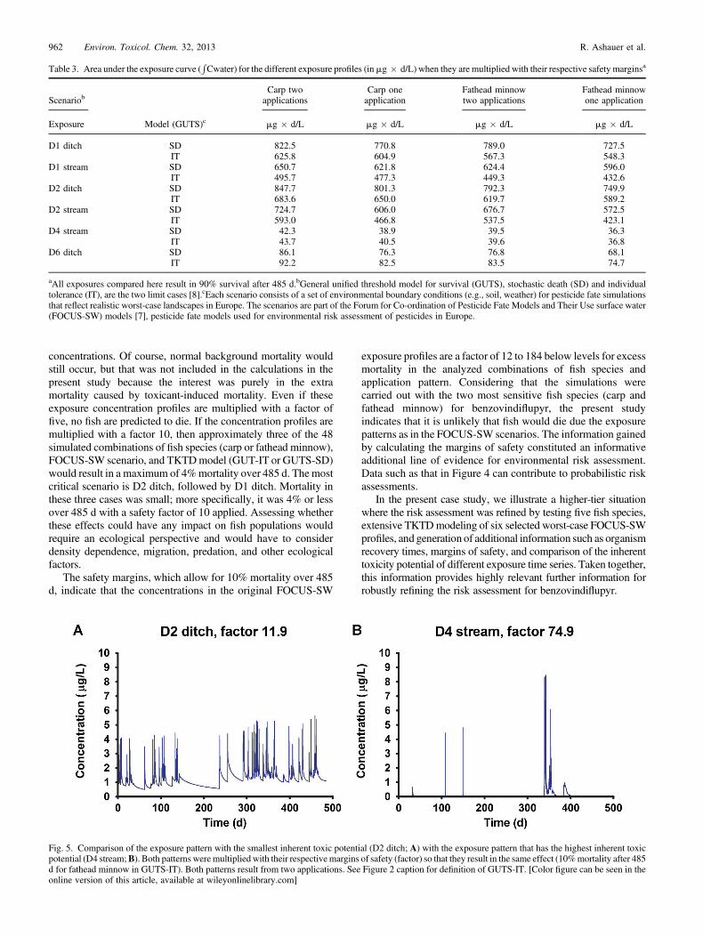
The areas under the exposure curves for the differentFOCUS-SW scenarios are shown in Table 3. All exposurepatterns were multiplied with their respective margin of safety toresult in 10%mortality after 485 d. The scenario D2 ditch had thelowest inherent toxic potential because it requires the largest areaunder the exposure curves to achieve 10%mortality. In contrast,D4 stream had the highest inherent toxic potential because itrequired the lowest area under the exposure curve to achieve10% mortality. In other words, if the PPP was applied inapplication rates such that scenarios D2 ditch and D4 stream had

the same area under the exposure curves, but preserved thecurrent shapes of the concentration time series, then D2 ditchwould be the least toxic and D4 stream would be the most toxicconcentration time series. Both FOCUS-SW scenarios areshown in Figure 5, and Table 4 summarizes the additionalcharacteristics calculated for each exposure pattern.

Sensitivity and uncertainty analysis

The sensitivity of the model depends on the exposure patternand differed between GUTS-IT and GUTS-SD (Fig. 6). Thesensitivity of survival after 485 d toward changes in theparameters alpha and beta of GUTS-IT were very similar in bothscenarios D2 ditch and D4 stream. However, the sensitivitytoward the parameters z and ke of the GUTS-SD model differedstrongly between the two exposure patterns. Because eachparameter was varied within its confidence limits, Figure 6 alsoindicates the maximum change in survival after 485 d that can beexpected due to the uncertainty of a single parameter. Figure 6clearly shows that this uncertainty also differs betweenparameters, model, and exposure scenario. For example, thelargest change in survival after 485 d was observed for changesin parameter z in the GUTS-SDmodel and the D2 ditch exposurepattern. In D4 stream, changes in z do not lead to large changes insurvival after 485 d.

Fig. 1. Model fit of general unified threshold model of survival–stochastic death (GUTS-SD; A,B) and general unified threshold model of survival–individualtolerance (GUTS-IT; C,D) [8] to the raw data from acute toxicity tests with carp (A,C) and fathead minnow (B,D). In both experiments, only the two highestconcentrations yielded mortalities. These concentrations were 5.4 mg/L (dotted line, diamonds) and 10 mg/L (solid line, triangles) for carp and 4.4 mg/L (dottedline, diamonds) and 9.4 mg/L (solid line, triangles) for fathead minnow. [Color figure can be seen in the online version of this article, available atwileyonlinelibrary.com]


DISCUSSION

Suitability of the model

The models GUTS-IT and GUTS-SD could be calibrated forbenzovindiflupyr and used to predict fish survival followingdifferent exposure patterns. There was no clear and consistentindication regarding which of the two models, GUTS-SD orGUTS-IT, better described the acute toxicity data for all five fishspecies. Both models should be used, therefore, as they are thetwo simplified, limited cases of GUTS. Several additionalcalculations could be performed, such as simulations withhigher exposure factors, calculations of organism recoverytimes and safety margins, and comparisons of exposure patternswith respect to their inherent toxic potential. Thus, comparedwith standard risk assessment where summary statistics ofconcentration–response curves are used, the models used in thepresent study could generate a wealth of additional informationand improve our understanding of the likely relationshipbetween fluctuating exposure patterns of benzovindiflupyr andtheir potential for toxic effects.

The models are calibrated with acute toxicity data fromexperiments of 4 d and then used to predict survival over 485 d

Fig. 2. Prediction of fry survival in the fathead minnow early life stagestudy. The model predicts mortality in excess of controls for the treatmentwith 4 mg/L (solid line, triangles), the highest tested concentration. Thereis a typical drop in survival between days 5 and 6, across treatment groups,as larvae transition to free feeding. GUTS-SD and GUTS-IT ¼ the twolimit cases of the general unified threshold model for survival (GUTS),including stochastic death (SD) and individual tolerance (IT) [8]. [Colorfigure canbe seen in the online version of this article, available atwileyonlinelibrary.com]

Table

2.Resultsof

simulated

fish

survival

inFOCUS-SW

exposure

patternsa

Scenariob

Model

(GUTS)

Carptwo

applications

Carptwo

applications

Carpone

application

Carpone

application

Fathead

minnow

twoapplications

Fathead

minnow

twoapplications

Fathead

minnow

oneapplication

Fathead

minnow

oneapplication

Endpoint

Survivalin

10�

higher

concentrations

(atday485)

Factor

(safetymargin)

Survivalin

10�

higher

concentrations

(atday485)

Factor

(safetymargin)

Survivalin

10�

higher

concentrations

(atday485)

Factor

(safetymargin)

Survivalin

10�

higher

concentrations

(atday485)

Factor

(safetymargin)

D1ditch

SD

100%

21.4

100%

52.4

100%

20.5

100%

49.5

IT100%

16.3

100%

41.1

99%

14.8

100%

37.3

D1stream

SD

100%

34.2

100%

85.9

100%

32.9

100%

82.3

IT100%

26.1

100%

65.9

100%

23.6

100%

59.7

D2ditch

SD

100%

16.3

100%

36.4

100%

15.3

100%

34.0

IT99%

13.2

100%

29.5

96%

11.9

100%

26.8

D2stream

SD

100%

28.3

100%

53.6

100%

26.4

100%

50.7

IT100%

23.2

100%

41.3

100%

21.0

100%

37.5

D4stream

SD

100%

80.0

100%

177

100%

74.7

100%

165

IT100%

82.7

100%

184

100%

74.9

100%

167

D6ditch

SD

100%

28.6

100%

61.8

100%

25.5

100%

55.1

IT100%

30.6

100%

66.8

100%

27.8

100%

60.5

a FOCUS-SW

aretheForum

forCo-ordinatio

nof

PesticideFateModelsandTheirUse

(FOCUS)surfacewater

models[7](pesticidefate

modelsused

forenvironm

entalrisk

assessmentof

pesticides

inEurope).

bEachscenario

consistsof

asetof

environm

entalboundary

conditions(e.g.,soil,

weather)forpesticidefate

simulations

that

reflectrealistic

worst-caselandscapes

inEurope.

GUTS¼

generalunified

thresholdmodel

forsurvival;SD

¼stochastic

death;

IT¼

individual

tolerance.


under different exposure scenarios. To our knowledge, such anextrapolation by any model has never been tested withindependent experimental data on fish survival over 485 d orsimilar. Within the present study, data from an ELS test withfathead minnows was used to test the predictive power of themodel over 28 d. The results indicated that the model is suitablefor estimating survival of fish following exposure tobenzovindiflupyr.

We used a one-compartment approximation, “reducedGUTS,” of an essentially two-compartment system comprisingTK and TD. The elimination rate of substances in fish dependson the size of the fish, which raises the question of whether thedominant rate constant ke also depends on the size of the fish.The model testing indicated that size differences between adultfathead minnow and fry do not preclude toxicity extrapolationfrom the adult to the fry. Nevertheless, the possible dependenceof ke and other GUTS parameters on organism traits needsfurther investigation, especially for traits such as organism sizethat change over time and under varying field conditions.

We carried out additional simulations to determine themargins of safety for the additional three species of fish (O.mykiss, C. variegatus, and L. macrochirus) in two scenarios(lowest and highest inherent toxicity potential: D2 ditch and D4stream, both with two applications). These simulations show thatcarp and fathead minnow have consistently lower margins ofsafety in those two fluctuating exposure profiles than the otherthree species (Supplemental Data). This demonstrates that carpand fathead minnow are more sensitive than the other tested fishspecies, not only under conditions of the LC50 toxicity test, butalso under fluctuating exposure conditions.

The scaled internal concentration in our reduced GUTSmodel stands for both the internal concentration (TK) and thedamage (TD) combined. It is important to realize that in thismodel, the decline of the scaled internal concentration, forexample after exposure, can be slower than the actual depurationof the substance if the recovery of the organism takes longer dueto lasting biochemical or physiological damage. The predictivepower of this so-called reduced GUTS model is equivalent tothat of the full GUTS model, which would include measuredtoxicokinetics [8,19].

Interpreting predicted survival and margins of safety

In the present case study, the simulationswith theTKTDmodelsshowed that none of the tested fish would die when exposed tobenzovindiflupyr over 485 d at the predicted FOCUS-SW

Fig. 3. Illustration of method: Simulations of fathead minnow survival with GUTS‐IT model in FOCUS‐SW model D2 ditch (A,D), in D2 ditch exposureconcentrations multiplied with factor 10 (B,E), and in D2 ditch exposure concentrations multiplied with factor 11.9 (margin of safety, 90% survival over 485 d;C,F). Graphs show predicted survival (A‐C) and concentrations in thewater body (D–F). FOCUS-SW ¼ Forum for Coordination of Pesticide FateModels and TheirUse (pesticide fate models used for environmental risk assessment in Europe) [7]. See Figure 2 caption for definition of GUTS-IT. [Color figure can be seen in theonline version of this article, available at wileyonlinelibrary.com]

Fig. 4. Margins of safety quantify how far below toxic levels the exposurepatterns are. Each group consists of 12 data points that result fromsimulations for the six FOCUS-SW scenarios analyzed with two models(GUTS-SD and GUTS-IT). See Figures 2 and 3 caption for definitions ofFOCUS-SW, GUTS-SD, and GUTS-IT.


concentrations. Of course, normal background mortality wouldstill occur, but that was not included in the calculations in thepresent study because the interest was purely in the extramortality caused by toxicant-induced mortality. Even if theseexposure concentration profiles are multiplied with a factor offive, no fish are predicted to die. If the concentration profiles aremultiplied with a factor 10, then approximately three of the 48simulated combinations of fish species (carp or fathead minnow),FOCUS-SW scenario, and TKTDmodel (GUT-IT or GUTS-SD)would result in a maximum of 4%mortality over 485 d. Themostcritical scenario is D2 ditch, followed by D1 ditch. Mortality inthese three cases was small; more specifically, it was 4% or lessover 485 d with a safety factor of 10 applied. Assessing whetherthese effects could have any impact on fish populations wouldrequire an ecological perspective and would have to considerdensity dependence, migration, predation, and other ecologicalfactors.

The safety margins, which allow for 10% mortality over 485d, indicate that the concentrations in the original FOCUS-SW

exposure profiles are a factor of 12 to 184 below levels for excessmortality in the analyzed combinations of fish species andapplication pattern. Considering that the simulations werecarried out with the two most sensitive fish species (carp andfathead minnow) for benzovindiflupyr, the present studyindicates that it is unlikely that fish would die due the exposurepatterns as in the FOCUS-SW scenarios. The information gainedby calculating the margins of safety constituted an informativeadditional line of evidence for environmental risk assessment.Data such as that in Figure 4 can contribute to probabilistic riskassessments.

In the present case study, we illustrate a higher-tier situationwhere the risk assessment was refined by testing five fish species,extensive TKTDmodeling of six selected worst-case FOCUS-SWprofiles, and generation of additional information such as organismrecovery times, margins of safety, and comparison of the inherenttoxicity potential of different exposure time series. Taken together,this information provides highly relevant further information forrobustly refining the risk assessment for benzovindiflupyr.

Table 3. Area under the exposure curve (RCwater) for the different exposure profiles (inmg � d/L) when they are multiplied with their respective safety marginsa

Scenariob

Model (GUTS)c

Carp twoapplications

Carp oneapplication

Fathead minnowtwo applications

Fathead minnowone application

Exposure mg � d/L mg � d/L mg � d/L mg � d/L

D1 ditch SD 822.5 770.8 789.0 727.5IT 625.8 604.9 567.3 548.3

D1 stream SD 650.7 621.8 624.4 596.0IT 495.7 477.3 449.3 432.6

D2 ditch SD 847.7 801.3 792.3 749.9IT 683.6 650.0 619.7 589.2

D2 stream SD 724.7 606.0 676.7 572.5IT 593.0 466.8 537.5 423.1

D4 stream SD 42.3 38.9 39.5 36.3IT 43.7 40.5 39.6 36.8

D6 ditch SD 86.1 76.3 76.8 68.1IT 92.2 82.5 83.5 74.7

aAll exposures compared here result in 90% survival after 485 d.bGeneral unified threshold model for survival (GUTS), stochastic death (SD) and individualtolerance (IT), are the two limit cases [8].cEach scenario consists of a set of environmental boundary conditions (e.g., soil, weather) for pesticide fate simulationsthat reflect realistic worst-case landscapes in Europe. The scenarios are part of the Forum for Co-ordination of Pesticide Fate Models and Their Use surface water(FOCUS-SW) models [7], pesticide fate models used for environmental risk assessment of pesticides in Europe.

Fig. 5. Comparison of the exposure pattern with the smallest inherent toxic potential (D2 ditch; A) with the exposure pattern that has the highest inherent toxicpotential (D4 stream;B). Both patterns weremultiplied with their respectivemargins of safety (factor) so that they result in the same effect (10%mortality after 485d for fathead minnow in GUTS-IT). Both patterns result from two applications. See Figure 2 caption for definition of GUTS-IT. [Color figure can be seen in theonline version of this article, available at wileyonlinelibrary.com]


Model sensitivity and uncertainty

Model sensitivity depends on the parameter, model (GUTS-SD or GUTS-IT), and exposure pattern (Figure 6). The fact thatmodel sensitivity depends on the exposure profile makes itdifficult to fully understand the uncertainty of our survivalpredictions and generalize conclusions about model sensitivity.The model is not very sensitive to changes in some parameters,

such as alpha and beta for GUTS-IT and kk for GUTS-SD,irrespective of which exposure pattern was used (D2 ditch orD4 stream). The model outcome is sensitive, however, tochanges in ke (both models) and especially z in GUTS-SD. Thesensitivity is more pronounced for D2 ditch than for D4 stream.This latter finding is related to the fact that D2 ditch containedmany short pulses throughout the entire 485-d period and alsoa continuous raised background concentration. In contrast, D4stream consisted of one main exposure event or exposureperiod only (see also Table 4). Thus, D2 ditch allows for amuch stronger interplay and repeated effects of changes in keand z on the simulated survival. This is simply because thereare more peaks that can lead to exceeding the threshold zand more intervals between peaks that could be too short or longenough for organism recovery. The sensitivity analysisimproves our understanding of the relationship betweenfluctuating exposure and toxic effect. However, the changessimulated in the present study that resulted from changes inone parameter at a time do not truly reflect the uncertainty inmodel predictions inherent in the parameters. This is the casebecause our one-at-a-time sensitivity analysis neglects the co-variation of parameters and, therefore, overestimates theuncertainty in model predictions. Thus, the confidence limitsof the model parameters quantify the outside boundary of theiruncertainty.

Table 4. Additional characteristics of each exposure profile

ScenarioaNumberof peaks

Mean intervalbetween peaks,

days

Mean durationof peaks,days

D1 ditch 20 22 19D1 stream 30 15 12D2 ditch 73 6 6D2 stream 109 4 3D4 stream 17 22 8D6 ditch 20 22 19

aEach scenario consists of a set of environmental boundary conditions (e.g.,soil, weather) for pesticide fate simulations that reflect realistic worst-caselandscapes in Europe. The scenarios are part of the Forum for Co-ordinationof Pesticide Fate Models and Their Use surface water (FOCUS-SW) models[7], pesticide fate models used for environmental risk assessment ofpesticides in Europe.

Fig. 6. Survival after 485 d as a function of variation in single parameter values within their confidence limits. Sensitivity of the GUTS-ITmodel (A,C) and GUTS-SDmodel (B,D). The sensitivity of themodel output to variation in parameter values differs for different exposure patterns (D2 ditch: upper panels, D4 stream: lower panels).See Figure 2 caption for definitions of GUTS-SD and GUTS-IT. [Color figure can be seen in the online version of this article, available at wileyonlinelibrary.com]


We did not propagate the parameter uncertainty through tothe model predictions. More sophisticated modeling techniques,such as parameter estimation with Monte Carlo Markov Chains,followed by forward Monte Carlo simulations with samplingfrom the chain, could be used to generate prediction intervalsaround the simulated survival. Such simulations could capturethe covariation of parameters in the model calibration andaccount for parameter covariation in the uncertainty analysis.

Model testing (validation) and testing needs

The results of the model validation using the ELS dataillustrate that GUTS-SD and GUTS-IT are able to predict themortality observed in fathead minnow fry. Exposing embryos inthe ELS is not modeled, and the model is calibrated to juvenile/adult fish sensitivity. Thus it might be expected that the modelwould predict less mortality than observed for the fry due to thegeneral expectations that early life stages are more sensitive thanjuvenile and adult fish [26]. As this was not the case thesesimulations strengthen the trust in predictions of the GUTS-SDand GUTS-IT model. Furthermore, because the model providedpredictions of ELS survival, it appears that sensitivity of the twofish life stages is similar.

In addition, it must be emphasized that the models werecalibrated first on acute toxicity studies and then tested bypredicting the outcome of the independent data derived from thelonger-term ELS study. Such a comparison (validation) is astrong test for the predictive power of a model and is notnormally part of the risk assessment procedure. Overall, thisvalidation against independent data (i.e., toxicity data not usedfor parameterization) provides evidence that the model is ableto reliably predict effects under different (longer) exposurepatterns.

In the present study, we use the GUTS models to predictsurvival over 485 d. It is desirable, but challenging in practice, totest the predictive capabilities of these models, or any alternativemodels, over such a long time span. Any alternative method ofrisk assessment of the FOCUS-SW exposure patterns makes anextrapolation from short-term tests to 485 d. This extrapolationstep is rarely stated explicitly, although inevitable, and theunderlying assumptions remain unclear and cannot be scruti-nized. The assumptions of the GUTS models, however, havebeen clearly stated and discussed [8]. Because data to testextrapolation models for fish survival over 485 d do not exist, forneither constant nor fluctuating or pulsed exposure, we cannotquantitatively evaluate the performance of any method,including GUTS.

One recent study found that different sets of calibration dataresult in different levels of agreement between survival data andGUTS predictions [19]. That study also found that GUTS-SDand GUTS-IT performed equally well and, more importantly,that models calibrated on acute toxicity data tended tooverestimate mortality under longer pulsed exposure conditions.This latter finding indicates that the method used in the presentstudy may err on the conservative side—that is, the safe side. Aforerunner model of GUTS has been calibrated and tested onindependent data [14,18]. The GUTS-type TKTD modelperformed at least as well as the alternative models, and in astudy with mixtures in time, it even predicted the effect of thesequence of exposure to two different compounds [18]. Theevidence available now indicates that GUTS predictions fortime-variable exposure are at least as reliable and, due to themore realistic model structure, quite possibly more trustworthythan alternative models.

Organism recovery, exposure patterns, and inherent toxicpotential

The predicted exposure pattern in D2 ditch for multipleexposure events is spread throughout the entire simulation period(Fig. 5), whereas predicted exposure in D4 stream shows onemajor event around day 350. Multiple exposure events, forexample in D2 ditch, allow the organisms to recover betweenpulses; thus, such a pattern has the lowest inherent toxicpotential. This must not be confused with the fact that D2 ditchwas the exposure pattern that is closest to the onset of mortality,as indicated by the lowest margins of safety (see Table 2). In theFOCUS-SW simulations, D2 ditch reaches comparatively highexposure concentrations. Thus, the high absolute exposure in D2ditch overcompensates for its low inherent toxic potential.

A comparison of organism recovery times with the intervalsbetween peaks can yield additional insight into the potentialtoxicity of the exposure profiles. The D4 stream scenario had thelowest number of peaks (Table 4), but none of the characteristicsyielded a clear pattern identifying the exposure profile with thelowest or highest inherent toxic potential. However, comparingthe mean interval between peaks (between 4 and 22 d) with theorganism recovery times (between 2 and 6 d) indicates that thefish, on average, will be able to recover between peaks; that is,the exposure events can be seen as toxicologically independent.Note that D2 stream, which has the shortest mean intervalbetween peaks (4 d) also has the shortest average peak duration(3 d), so that, on average, recovery is also plausible in the presentstudy, even though there are 109 peaks over the period of 485 d.Comparing the D2 ditch and D4 stream also demonstrates thatfor benzovindiflupyr, toxicity is not simply a function of the areaunder the exposure curve, because the areas under the curvesdiffer widely for different patterns that result in the same overalleffect (see Table 3).

Use in higher tier risk assessment for registration of PPPs

The use of TKTD modeling, in particular predicting survivalusing GUTS, supplements existing environmental risk assess-ment methods well because carry-over effects and delayedtoxicity can be simulated. Furthermore, using the two extremecases, GUTS-SD and GUTS-IT, increases the confidence in therisk assessments because these two generic models apply to allmechanisms of toxicity. The question regarding which margin ofsafety is acceptable and which percentage of mortality insimulations with certain exposure factors would be acceptableremains a risk management question. Any use of short-termtoxicity data to arrive at risk assessment decisions for the 485-dFOCUS-SW exposure patterns requires assumptions andunderlying models, and these are rarely stated explicitly orjustified. Thus, the clear communication of underlying assump-tions of GUTS [8] increases transparency and under-standing of the risk assessment process. In addition, theanalysis presented in the present study makes use of the rawdata from the acute toxicity test; thus, it extracts moreinformation than summary statistics such as LC50 values andfacilitates extrapolations that are not possible with LC50 basedpredictions alone.

The toxic potency of fluctuating or pulsed exposures cannotbe known a priori. Rather, the interplay of longer, lowconcentrations and shorter, high concentrations resulted in anon-linear relationship with toxicity, which is specific to eachcombination of species and test substance. As the survivalprediction with GUTS can also identify which parts of the


exposure profile are potentially most toxic to organisms, suchanalyses can also guide more targeted mitigation measures.

CONCLUSION

Taking time-variable exposure explicitly into account viaTKTDmodeling improves our understanding of the relationshipbetween fluctuating exposure and toxicity. The GUTS iscurrently the best tool when the endpoint is survival. Theadditional information and insight gained through TKTDmodeling and careful analysis of the exposure patterns canstrengthen the environmental risk assessment of PPPs.

SUPPLEMENTAL DATA

Model calibration and parameter estimates for threeadditional fish species as well as a comparison of survivalunder fluctuating exposure for all five fish species.

Tables S1 to S7.Figs. S1 to S6. (201 KB PDF).

Acknowledgement—R. Ashauer was contracted and paid by Syngenta tocarry out the present study. We thank P. Rainbird for his contribution to thepresent study.

REFERENCES

1. Kreuger J. 1998. Pesticides in stream water within an agriculturalcatchment in southern Sweden, 1990–1996. Sci Total Environ 216:227–251.

2. Wittmer IK, Bader HP, Scheidegger R, Singer H, Lück A, Hanke I,Carlsson C, Stamm C. 2010. Significance of urban and agricultural landuse for biocide and pesticide dynamics in surface waters. Water Res44:2850–2862.

3. Brock TCM, Alix A, Brown CD, Capri E, Gottesbüren B, Heimbach F,Lythgo CM, Schulz R, StrelokeM. eds. 2010. Linking Aquatic Exposureand Effects. Society of Environmental Toxicology and Chemistry,Pensacola, FL, USA.

4. Reinert KH, Giddings JA, Judd L. 2002. Effects analysis of time-varyingor repeated exposures in aquatic ecological risk assessment ofagrochemicals. Environ Toxicol Chem 21:1977–1992.

5. Ashauer R, Boxall ABA, Brown CD. 2006. Predicting effects on aquaticorganisms from fluctuating or pulsed exposure to pesticides. EnvironToxicol Chem 25:1899–1912.

6. Ashauer R, Wittmer I, Stamm C, Escher BI. 2011. Environmental riskassessment of fluctuating diazinon concentrations in an urban andagricultural catchment using toxicokinetic-toxicodynamic modeling.Environ Sci Technol 45:9783–9792.

7. Forum for Co-ordination of Pesticide Fate Models and Their Use(FOCUS). 2001. FOCUS surface water scenarios in the EU evaluationprocess under 91/414/EEC. Report prepared by the FOCUS WorkingGroup on Surface Water Scenarios. European Commission, Health &Consumer Protection Directorate-General, Brussels, Belgium

8. Jager T, Albert C, Preuss TG, Ashauer R. 2011. General unifiedthreshold model of survival: A toxicokinetic-toxicodynamic frameworkfor ecotoxicology. Environ Sci Technol 45:2529–2540.

9. Ashauer R, Escher BI. 2010. Advantages of toxicokinetic andtoxicodynamic modelling in aquatic ecotoxicology and risk assessment.J Environ Monitor 12:2056–2061.

10. Jager T. 2011. Some good reasons to ban ECx and related concepts inecotoxicology. Environ Sci Technol 45:8180–8181.

11. Jager T, Heugens EHW, Kooijman SALM. 2006. Making sense ofecotoxicological test results: Towards application of process-basedmodels. Ecotoxicology 15:305–314.

12. Ashauer R, Agatz A, Albert C, Ducrot V, Galic N, Hendriks J, Jager T,Kretschmann A, O'Connor I, Rubach MN, Nyman A-M, Schmitt W,Stadnicka J, Van den Brink PJ, Preuss TG. 2011. Toxicokinetic-toxicodynamic modeling of quantal and graded sublethal endpoints: Abrief discussion of concepts. Environ Toxicol Chem 30:2519–2524.

13. Ashauer R, Hintermeister A, Caravatti I, Kretschmann A, Escher BI.2010. Toxicokinetic-toxicodynamic modeling explains carry-overtoxicity from exposure to diazinon by slow organism recovery. EnvironSci Technol 44:3963–3971.

14. Ashauer R, Boxall ABA, BrownCD. 2007. New ecotoxicological modelto simulate survival of aquatic invertebrates after exposure to fluctuatingand sequential pulses of pesticides. Environ Sci Technol 41:1480–1486.

15. Stadnicka J, Schirmer K, Ashauer R. 2012. Predicting concentrations oforganic chemicals in fish by using toxicokinetic models. Environ SciTechnol 46:3273–3280.

16. Hommen U, Ashauer R, Van den Brink P, Caquet T, Ducrot V, LagadicL, Ratte HT. 2010. Extrapolation methods in aquatic effects assessmentof time-variable exposures to pesticides. In Brock TCM, Alix A, BrownCD, Capri E, Gottesbüren B, Heimbach F, Lythgo CM, Schulz R,Streloke M, eds, Linking Aquatic Exposure & Effects in the RiskAssessment of Pesticides. Society of Environmental Toxicology andChemistry, Pensacola, FL, USA, pp 211–242.

17. Altenburger R, Greco WR. 2009. Extrapolation concepts for dealingwith multiple contamination in environmental risk assessment. IntegrEnviron Assess Manag 5:62–68.

18. Ashauer R, Boxall ABA, Brown CD. 2007. Modeling combined effectsof pulsed exposure to carbaryl and chlorpyrifos on Gammarus pulex.Environ Sci Technol 41:5535–5541.

19. Nyman A-M, Schirmer K, Ashauer R. 2012. Toxicokinetic-toxicody-namic modelling of survival of Gammarus pulex in multiple pulseexposures to propiconazole: Model assumptions, calibration datarequirements and predictive power. Ecotoxicology 21:1828–1840.

20. Ashauer R. 2010. Toxicokinetic-toxicodynamic modelling in anindividual based context—Consequences of parameter variability.Ecol Model 221:1325–1328.

21. Zhao Y, Newman MC. 2007. The theory underlying dose–responsemodels influences predictions for intermittent exposures. EnvironToxicol Chem 26:543–547.

22. Kooijman SALM, Bedaux JJM. 1996. Some statistical properties ofestimates of no-effect concentrations. Water Res 30:1724–1728.

23. Organisation for Economic Co-operation and Development (OECD).1992. OECD guidelines for testing chemicals 210: Fish, early-life stagetoxicity test. Paris, France.

24. Ashauer R, Boxall ABA, Brown CD. 2007. Simulating toxicity ofcarbaryl to Gammarus pulex after sequential pulsed exposure. EnvironSci Technol 41:5528–5534.

25. Ashauer R, Brown CD. 2007. Comparison between FOCUS output forpesticide concentrations over time and field observations. Report forDEFRA project DS 3321. The University of York, York, UK.

26. McKim JM. 1977. Evaluation of tests with early life stages of fish forpredicting long-term toxicity. J Fish Res Board Can 34:1148–1154.


a method to predict and understand fish survival … · a method to predict and understand fish...

Documents