a mixed integer linear programming based load shedding
TRANSCRIPT

sustainability
Article
A Mixed Integer Linear Programming Based LoadShedding Technique for Improving the Sustainabilityof Islanded Distribution Systems
Sohail Sarwar 1, Hazlie Mokhlis 1,* , Mohamadariff Othman 1, Munir Azam Muhammad 1,J. A. Laghari 2, Nurulafiqah Nadzirah Mansor 1, Hasmaini Mohamad 3 and Alireza Pourdaryaei 1,4
1 Department of Electrical Engineering, Faculty of Engineering, University of Malaya,Kuala Lumpur 50603, Malaysia; [email protected] (S.S.); [email protected] (M.O.);[email protected] (M.A.M.); [email protected] (N.N.M.);[email protected] (A.P.)
2 Department of Electrical Engineering, Quaid-e-Awam University of Engineering Science and Technology,Nawabshah, Sindh 67480, Pakistan; [email protected]
3 Faculty of Electrical Engineering, University of Technology Mara, Shah Alam 40450, Malaysia;[email protected]
4 Department of Electrical and Computer Engineering, University of Hormozgan,Bandar Abbas 7916193145, Iran
* Correspondence: [email protected]
Received: 22 June 2020; Accepted: 29 July 2020; Published: 3 August 2020�����������������
Abstract: In recent years significant changes in climate have pivoted the distribution system towardsrenewable energy, particularly through distributed generators (DGs). Although DGs offer manybenefits to the distribution system, their integration affects the stability of the system, which couldlead to blackout when the grid is disconnected. The system frequency will drop drastically if DGgeneration capacity is less than the total load demand in the network. In order to sustain the systemstability, under-frequency load shedding (UFLS) is inevitable. The common approach of load sheddingsheds random loads until the system’s frequency is recovered. Random and sequential selectionresults in excessive load shedding, which in turn causes frequency overshoot. In this regard, thispaper proposes an efficient load shedding technique for islanded distribution systems. This techniqueutilizes a voltage stability index to rank the unstable loads for load shedding. In the proposedmethod, the power imbalance is computed using the swing equation incorporating frequency value.Mixed integer linear programming (MILP) optimization produces optimal load shedding strategybased on the priority of the loads (i.e., non-critical, semi-critical, and critical) and the load rankingfrom the voltage stability index of loads. The effectiveness of the proposed scheme is tested on twotest systems, i.e., a 28-bus system that is a part of the Malaysian distribution network and the IEEE69-bus system, using PSCAD/EMTDC. Results obtained prove the effectiveness of the proposedtechnique in quickly stabilizing the system’s frequency without frequency overshoot by disconnectingunstable non-critical loads on priority. Furthermore, results show that the proposed technique issuperior to other adaptive techniques because it increases the sustainability by reducing the loadshed amount and avoiding overshoot in system frequency.
Keywords: unprecedented frequency variations; distributed generation; cascaded blackout; loadpriority; stability index of loads; mixed integer linear programming; frequency overshoot
Sustainability 2020, 12, 6234; doi:10.3390/su12156234 www.mdpi.com/journal/sustainability
Sustainability 2020, 12, 6234 2 of 23
1. Introduction
The electrical power system is at the epicenter of any country’s economic development.Conventionally, electricity is generated in bulk from fossil fuels and transmitted to consumers.This convention ensures security of supply and reliability; however, it is the cause of one-third ofworld’s total greenhouse gas (GHC) emissions [1]. Alternatively, renewable energy resources (RES)generate emission-free electrical power and are projected to reduce GHG emissions to less than 80% bythe year 2050 [2]. In addition, GHG emission and electricity consumption are correlated in which aone-degree increment in ambient temperature due to emissions will result in an increase in electricityconsumption per person between 0.5% and 0.85% [3]. This phenomenon is one of the driving forcesbehind the inclination towards the integration of distributed generators (DGs) based on renewablesources to achieve universal energy access by 2030 [4,5].
Despite numerous advantages, DGs have their own limitations [6]. A grid-connected DGusually has as its capacity less than the total load demand of the network. Frequency instabilityis a common occurrence in the event of islanded operation of the DG, which affects consumersdownstream [7,8]. However, load shedding can be initiated to prevent further blackout [9].Conventional load shedding entails disconnecting predefined loads from the power supply throughunder-frequency relay [10]. The setting of the relay depends on the degree to which the frequencyhas declined [11,12]. Adaptive settings for under-frequency relay settings were proposed in [13].This technique optimizes the frequency setpoint, time delay, and load shed amount for each step usingmixed-integer linear programming. However, it can be observed from the result that the load sheddingtechnique performs excessive disconnection of the load that causes overshoot in the frequency response.On the other hand, semi-adaptive load shedding involves calculating the power imbalance usingfrequency response to determine the appropriate number of loads to be shed. This is achieved bycalculating the second derivative of the frequency based on Newton’s method approximation [14,15].The system frequency response identified from phasor measurement units is used in [16] to form a newmultistage load shedding scheme. Imperialist competitive algorithm, an application of evolutionaryprogramming, evaluates the estimates of the load to be shed. This technique analyzes the under- orover-shedding in multiple stages to validate the recovery level of the system frequency. Although theseprevious schemes improve the frequency response and open up new paths for load shedding,predetermined frequency thresholds and sequential selection of loads result in un-optimized loadshedding. Furthermore, the threshold value also needs to be changed when the system is upgraded.
Unlike conventional techniques, computational intelligence-based techniques can measure andpredict the power imbalance more accurately and result in a better solution for load shedding.Hooshmand et al. [17] proposed such an adaptive technique for under-frequency load shedding(UFLS) using an artificial neural network (ANN). The ANN model together with appropriate dataanalysis is capable of minimizing load shedding compared to conventional techniques in steps of10%, 20%, and 25% of the total load with 0.1 s of delay in each step. This technique opened anew frontier for UFLS techniques for the researchers. Instantaneous and average rate of change ofsystem frequency is used in another technique to train the ANN network. Load equal to the valueof the calculated power imbalance is shed from the system using a relay in [18]. A new methodfor load shedding was also proposed in [19] using ANN and a hybrid co-evolutionary algorithm,culture-particle swarm optimization. The scheme produces a more accurate solution in a faster timecompared to the conventional schemes. Additionally, the scheme calculates the active as well asreactive power to be shed in each predefined step. Monte Carlo Simulation (MCS) is also employedfor the load shedding problem in [20] to find generation deficiency to shed the loads accordinglyusing four different load shedding scenarios, i.e., increasing, decreasing, equal block, and a sandwichplan employing predefined frequency relay setting in five steps. The employment of fuzzy logic foraccurate measurement of the power imbalance has also gained traction in the past. A fuzzy-basedload shedding scheme for a small university distribution system is implemented in [21]. UFLS-basedon fuzzy logic is tested for a steam-driven sugar industry plant in which steam input and frequency
Sustainability 2020, 12, 6234 3 of 23
deviation are considered as the inputs. The algorithm generates two-layer outputs that decide loads tobe shed on load cluster and number of loads. The method minimizes the load shed in comparison toconventional UFLS in [22]. The distribution state estimator in [23] measures the power consumptionon each bus using historical data and load flow analysis. Event and frequency calculator modules areused to estimate the power imbalance, and loads are shed one by one, according to the priority for adistribution test system of 102 buses.
From the above literature review of various schemes for UFLS, it is evident that forecast of powerimbalance using ANN, MCS, and fuzzy logic anticipates more accurate estimates. However, loadshedding is executed in a conventional approach that results in an overshoot in the system frequencyresponse (SFR) due to excessive load shedding. Prioritized selection of non-critical or more unstableloads is a better alternative to the conventional approach of sequential selection. Location andthe type of disturbance have a significant effect on system stability and load shedding [24], whichwas not investigated in the techniques discussed above. The stability index of loads for differentdisturbances is a vital factor; a study in [25] showed that prioritization of loads utilizing fuzzylogic considering social, economic, or political aspects of connected loads can further improve theresponse. Estimation of stability indices of loads [26,27] to prefer unstable loads for sheddingresults in an improved voltage profile of the system, avoiding operation of undervoltage protection.Sequential selection of loads in [26,27] results in frequency overshoot due to excessive shedding,despite prioritizing the loads. Therefore, finding an optimal combination of loads to be shed is analternative approach to sequential selection.
In order to improve the frequency response, the combination selection approach based on anexhaustive search was proposed to find the best combination that matches the power imbalance in thesystem [28]. However, this technique is only suitable for a small number of loads in the system, since itwill be time-consuming for a larger-scale system. In [29], a meta-heuristic technique was used to findthe best combination of random priority loads. The technique takes more time to find the optimalsolution, especially when the number of loads is increased.
In view of the aspects discussed above, it can be summarized that conventional techniques resultin excessive load shedding due to predefined relay settings, whereas the practical implementation ofcomputational intelligence-based techniques is still questionable for utility grids [30]. On the otherhand, UFLS techniques based on the stability index increase the voltage stability by detaching the moreunstable loads on priority. However, sequential selection of unstable loads hinders the accuracy ofsuch techniques and produces overshoot in frequency. Therefore, a new efficient load shedding schemeis proposed in this paper. The optimal load combination from unstable non-critical and semi-criticalloads is found using mixed-integer linear programming (MILP) optimization. The main contributionsof this paper are:
The reliability of the system is increased by prioritized selection of non-critical loads to ensuresupply to semi-critical and critical loads, although load shedding is initiated.
1. The stability of the system voltage and frequency is improved by prioritizing the loads based ontheir stability index so that more unstable load buses are disconnected on priority.
2. Mathematical modeling-based strategy for optimal selection of loads from unstable and non-criticalloads to be shed using MILP to improve frequency response with minimum frequency overshootduring islanded operation of the distribution system connected with the DGs.
The rest of this paper is arranged as follows: Section 2 demonstrates the proposed methodologyand Section 3 explains the modeling of the system under observation. Results and Discussions areillustrated in Sections 4 and 5. Section 6 concludes the research paper.
2. Methodology
This research aims to propose a new UFLS technique that yields an optimal solution for thefrequency stabilization of an islanded distribution system. The working principle of the proposed
Sustainability 2020, 12, 6234 4 of 23
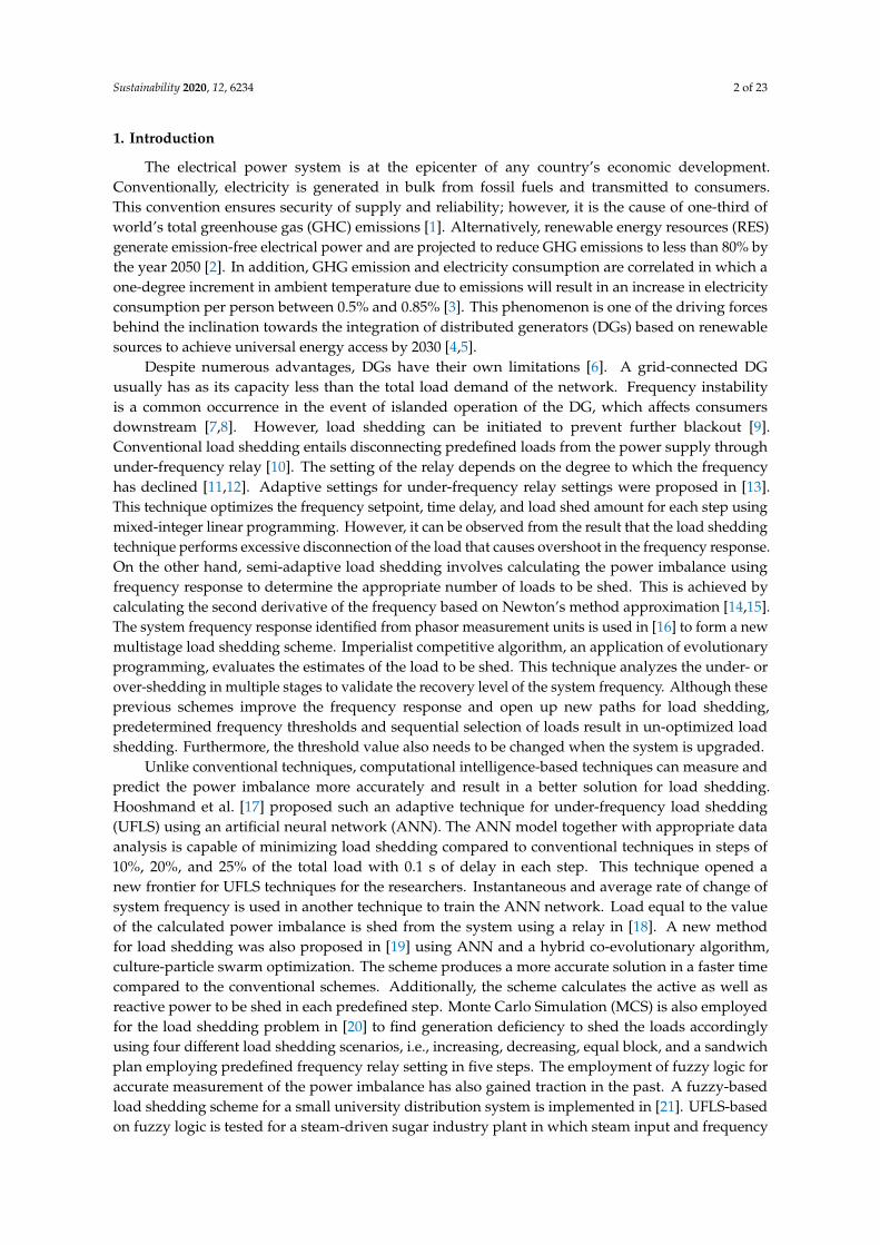
technique is explained in a block diagram shown in Figure 1. The proposed technique in this papercomprises four modules:
• Average system frequency calculation module• Power imbalance calculation module• Stability index calculation module• Intelligent load shedding module
Sustainability 2020, 12, x FOR PEER REVIEW 4 of 23
Sustainability 2020, 12, x; doi: FOR PEER REVIEW www.mdpi.com/journal/sustainability
Power imbalance calculation module
Stability index calculation module
Intelligent load shedding module
Figure 1. Block diagram of the proposed load shedding scheme.
The working of all above modules is explained in the following sections.
2.1. Average System Frequency Calculation Module
The basic parameter of any load shedding scheme is frequency. In grid-connected mode, the
grid controls the system frequency with DGs supplying some of the load demands. However, in
islanded mode, the system frequency will behave abnormally. Furthermore, the inertia constant,
spinning reserve, and turbine control mechanism of each DG further alter the system frequency.
Thus, an average system frequency needs to be considered during islanded mode as presented in
Equation (1):
1
1
M
i i
isys M
i
i
H f
f
H
, (1)
where Hi is the inertia constant of the ith generator in seconds, fi is the frequency of the ith generator,
and M is the number of DGs connected in the system. The rate of change of system frequency is
evaluated from the derivative of fsys. This decaying frequency information is used to calculate the
power imbalance in the system.
2.2. Power Imbalance Calculation Module (PICM)
The PICM calculates the power imbalance in the system and subsequently the equivalent
amount of load to be shed following any system changes that cause frequency drop. A grid-coupling
circuit breaker continuously monitors the condition of the system and indicates an islanding event
when it happens. In this case, the tripping of any circuit breaker coupling a DG to the distribution
system in islanding condition is recorded as a DG-tripping event. The total power imbalance, ∆P in
the system for such a scenario, is calculated using Equation (2), considering the spinning reserves of
the generators.
PbiomassBiomass DG
Distribution
system
Pgrid
Grid fsys & df/dt
PLi
CB status
PI
CBCBCB
CBCB
Load Load
LoadLoadLoad
Power Imbalance
Calculation Module
Stability index
module
P, Q, R, X and Vs
SIi
Intelligent Load
Shedding Module
Hydro DG 2
PHydro2
PHydro1Hydro DG 1
Average system
frequency Calculation
module
fDGs HDGs
Figure 1. Block diagram of the proposed load shedding scheme.
The working of all above modules is explained in the following sections.
2.1. Average System Frequency Calculation Module
The basic parameter of any load shedding scheme is frequency. In grid-connected mode, the gridcontrols the system frequency with DGs supplying some of the load demands. However, in islandedmode, the system frequency will behave abnormally. Furthermore, the inertia constant, spinningreserve, and turbine control mechanism of each DG further alter the system frequency. Thus, an averagesystem frequency needs to be considered during islanded mode as presented in Equation (1):
fsys =
M∑i=1
Hi · fi
M∑i=1
Hi
, (1)
where Hi is the inertia constant of the ith generator in seconds, fi is the frequency of the ith generator,and M is the number of DGs connected in the system. The rate of change of system frequency isevaluated from the derivative of fsys. This decaying frequency information is used to calculate thepower imbalance in the system.
2.2. Power Imbalance Calculation Module (PICM)
The PICM calculates the power imbalance in the system and subsequently the equivalent amountof load to be shed following any system changes that cause frequency drop. A grid-coupling circuitbreaker continuously monitors the condition of the system and indicates an islanding event when it
Sustainability 2020, 12, 6234 5 of 23
happens. In this case, the tripping of any circuit breaker coupling a DG to the distribution system inislanding condition is recorded as a DG-tripping event. The total power imbalance, ∆P in the system forsuch a scenario, is calculated using Equation (2), considering the spinning reserves of the generators.
∆P =N∑
i=1
PLi −
z·PGrid +M∑
i=1
PDGi
− (1− z)·PSR (2)
∆P in Equation (2) is the power imbalance of the system, N is the total number of loads in thesystem, M is the total number of DGs connected in the system, PGrid is the grid power, PLi is thereal-time load value at bus i, PDGi is the total dispatched power of DGi and PSR is the total spinningreserves in the system, whereas z in the above equation is a binary variable to indicate the operationalstate of the distribution system. A value of 1 for variable z indicates grid-connected mode and 0 valueindicates the islanded mode. Spinning reserves PSR is the total maximum capacity of the DGs atwhich they can operate without violating the frequency limits. These reserves must be utilized whiledesigning load shedding schemes, which can be calculated by Equation (3).
PSR =M∑
i=1
MaxDGi −
M∑i=1
PDGi (3)
where MaxDGi is the maximum generation capacity of DGi. On the other hand, a sudden connectionof loads into the stabled islanded distribution system may significantly change the system frequency,resulting in a power imbalance condition that might not be captured by Equation (3). In this regard,power imbalance ∆P in the system for such scenarios can be computed using the following equation:
∆P =
2×
M∑i=1
Hifn
× d( fsys)
dt
(4)
where Hi is the inertia constant of the ith generator in seconds, fn is the nominal frequency, and d(fsys)/dtis the rate of change of the system frequency. This PICM can monitor all the changes in the system.The power imbalance threshold level is set to be equivalent to the smallest value of the active powerload in the distribution system, which is 0.05 MW in the case studies, to avoid unnecessary activationof the load shedding scheme. In the case that the power imbalance is more than the set threshold level,the same power imbalance value will be passed over to the intelligent load shedding module (ILSM)for shedding of an equivalent amount of load. Moreover, this module will transmit an activation signalto the stability index calculation module (SICM) to estimate the stability indices of load buses.
2.3. Stability Index Calculation Module (SICM)
The stability index of a bus in a distribution system depends upon the connected load and thesending end voltage to that bus. Furthermore, it also depends upon the impedance of that distributionline [31]. This module will capture real-time sending end voltage, load, and impedance values ofeach bus when the activation signal from the PICM is received. The stability index for this scheme iscalculated using Equation (5), which was proposed in [31] and utilized for load shedding in [27].
SIi = (Vsi)4− 4(Pi.Ri −Qi.Xi)
2− 4(Pi.Xi −Qi.Ri).(Vsi)
2 (5)
where SIi is stability index of the ith load bus, Pi, Qi, Ri, Xi, and Vsi are active power, reactive power,resistance, reactance, and sending end voltage, respectively, for the ith bus. The stability indicescalculated in this module are then transmitted to the ILSM for activating optimal load shedding selection.

Sustainability 2020, 12, 6234 6 of 23
2.4. Intelligent Load Shedding Module (ILSM)
The ILSM provides an optimal solution for load shedding, where it captures the real-time load valuesfrom PSCAD. These loads have been categorized as non-critical, semi-critical, and critical loads. The powerimbalance forecasted in the PICM is analyzed and a combination of loads for shedding if the powerimbalance is greater than Pthreshold is determined by solving the MILP optimization. The MILP modeland objective function of the problem are shown in canonical form, Equation (6) is the objective function,Equations (7) and (8) are constraints to follow, and Equations (9) and (10) present parameter limits.
OF = min∑
j∈NCL
α.SI j.x j +∑
k∈SCL
β.SIk.xk +∑l∈CL
γ.SIl.xl + δ.w (6)
Subject toN∑
i=1(xi.PLi) −w ≤ PI ∀PLi ≥ 0 (7)
N∑i=1
{xi.(−PLi)
}−w ≤ (−PI) ∀PLi ≥ 0 (8)
α, β,γ and δ are non negative numbers (9)
xi =
{01
DisconnectedConnected
∀i = 1, 2, 3 · · ·N (10)
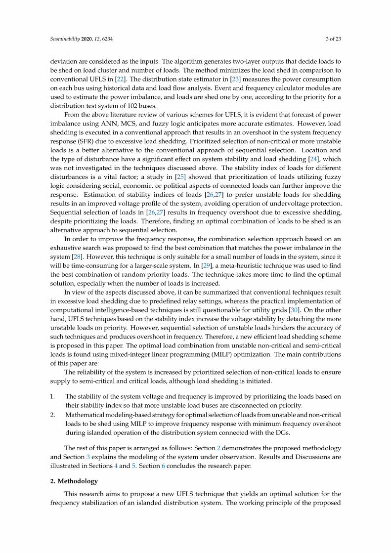
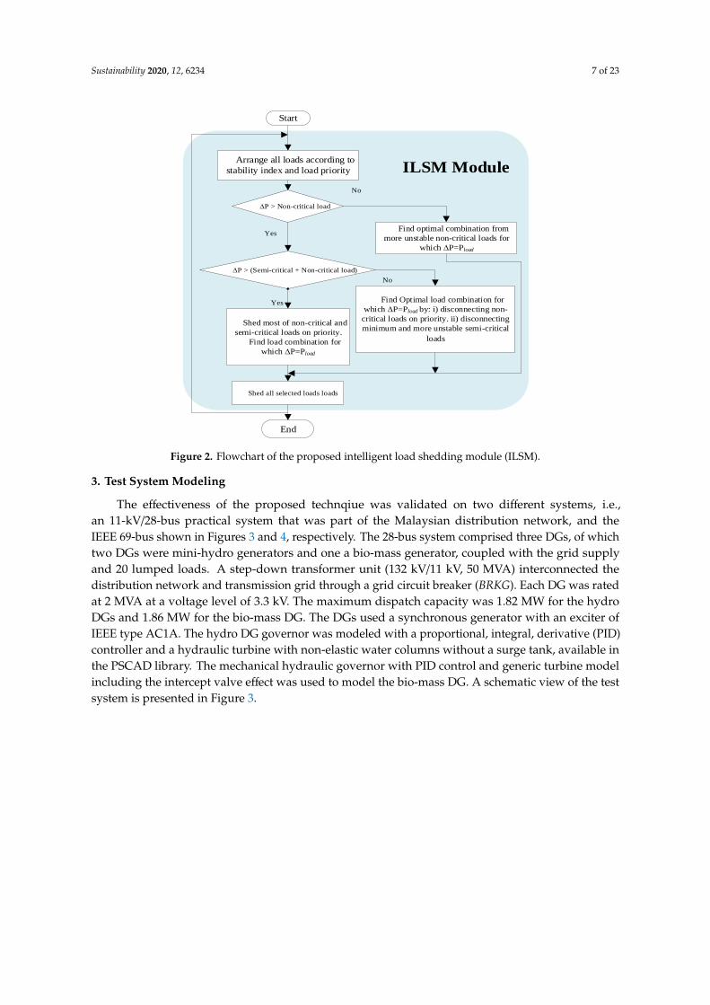
where PLi is the real-time load value at bus i, N is the total number of loads in the system, SI isthe stability index of the load, NCL, SCL, and CL are noncritical, semi-critical and critical load sets,respectively, and the binary variable x takes a value of 1 if the load’s circuit breaker disconnects the loadfrom the system, 0 otherwise. α, β, and γ are coefficients of the linear problem for load priority andoptimization These values are calculated so that the model should not select any additional semi-criticalor critical load and only shed the non-critical loads. w in the objective function is a dummy variableand δ is its coefficient. The objective function is to minimize the difference of the estimated powerimbalance, and ideally it should be 0. However, it cannot be 0 for all possible scenarios, therefore,a dummy variable is needed to satisfy the designed constraints in certain conditions. Its coefficient δ isgiven a very high value so that the objective function minimizes this dummy variable value. The blockdiagram of this module is shown in Figure 2.
This module finds the optimal combination of loads to be shed to match the power imbalance ofthe system with minimum error, incorporating stability indices of loads and load priority. The followingconditions are performed during the load shedding process:
(1) A combination of only non-critical and more unstable loads will be shed if the power mismatch isless than the total non-critical load in the system.
(2) If the power mismatch is more than the total amount of non-critical loads in the system, the modulewill shed an optimal combination of more unstable non-critical and semi-critical loads to matchthe power imbalance in the system. However, non-critical loads will be shed on priority.
(3) Lastly, if the power imbalance is more than the amount of non-critical plus the semi-critical loads,all the non-critical and semi-critical loads will be shed and an optimal combination of criticalloads will be determined for balancing the load and supply. It is a better solution to disconnect afew of the critical loads instead of total blackout in case of extreme contingency.
Sustainability 2020, 12, 6234 7 of 23
Sustainability 2020, 12, x FOR PEER REVIEW 6 of 23
Sustainability 2020, 12, x; doi: FOR PEER REVIEW www.mdpi.com/journal/sustainability
optimization. The MILP model and objective function of the problem are shown in canonical form,
Equation (6) is the objective function, Equations (7) and (8) are constraints to follow, and Equations
(9) and (10) present parameter limits.
min . . . . . . .j j k k l l
j NCL k SCL l CL
OF SI x SI x SI x w
(6)
Subject to
1
( . ) 0N
i i i
i
x PL w PI PL
(7)
1
. 0N
i i i
i
x PL w PI PL
(8)
, , and are non negative numbers (9)
01,2,3
1i
Disconnectedx i N
Connected
(10)
where PLi is the real-time load value at bus i, N is the total number of loads in the system, SI is the
stability index of the load, NCL, SCL, and CL are noncritical, semi-critical and critical load sets,
respectively, and the binary variable x takes a value of 1 if the load’s circuit breaker disconnects the
load from the system, 0 otherwise. α, β, and γ are coefficients of the linear problem for load priority
and optimization These values are calculated so that the model should not select any additional semi-
critical or critical load and only shed the non-critical loads. w in the objective function is a dummy
variable and δ is its coefficient. The objective function is to minimize the difference of the estimated
power imbalance, and ideally it should be 0. However, it cannot be 0 for all possible scenarios,
therefore, a dummy variable is needed to satisfy the designed constraints in certain conditions. Its
coefficient δ is given a very high value so that the objective function minimizes this dummy variable
value. The block diagram of this module is shown in Figure 2.
Figure 2. Flowchart of the proposed intelligent load shedding module (ILSM).
Start
P > Non-critical load
Arrange all loads according to
stability index and load priority
P > (Semi-critical + Non-critical load)
Shed most of non-critical and
semi-critical loads on priority.
Find load combination for
which P=Pload
Shed all selected loads loads
End
Yes
Yes
Find optimal combination from
more unstable non-critical loads for
which P=Pload
No
No
Find Optimal load combination for
which P=Pload by: i) disconnecting non-
critical loads on priority. ii) disconnecting
minimum and more unstable semi-critical
loads
ILSM Module
Figure 2. Flowchart of the proposed intelligent load shedding module (ILSM).
3. Test System Modeling
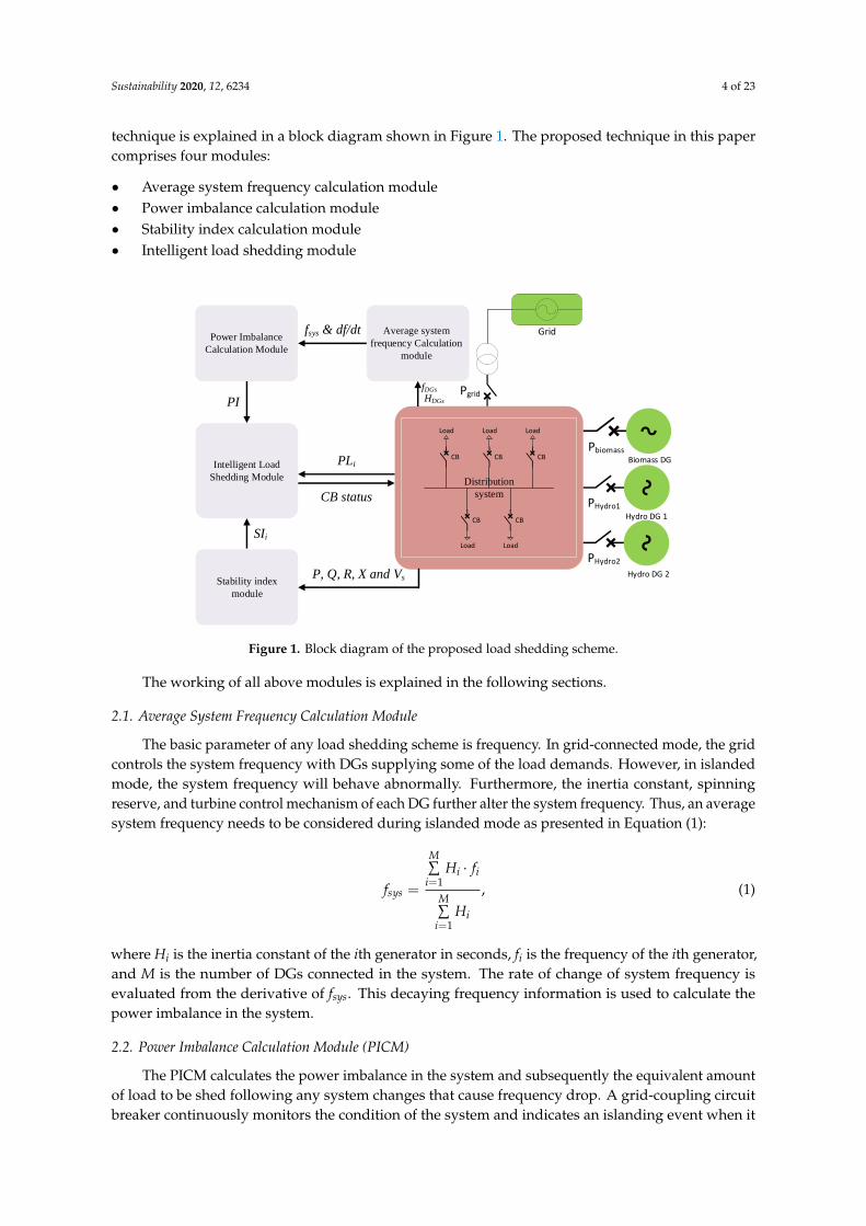
The effectiveness of the proposed technqiue was validated on two different systems, i.e.,an 11-kV/28-bus practical system that was part of the Malaysian distribution network, and theIEEE 69-bus shown in Figures 3 and 4, respectively. The 28-bus system comprised three DGs, of whichtwo DGs were mini-hydro generators and one a bio-mass generator, coupled with the grid supplyand 20 lumped loads. A step-down transformer unit (132 kV/11 kV, 50 MVA) interconnected thedistribution network and transmission grid through a grid circuit breaker (BRKG). Each DG was ratedat 2 MVA at a voltage level of 3.3 kV. The maximum dispatch capacity was 1.82 MW for the hydroDGs and 1.86 MW for the bio-mass DG. The DGs used a synchronous generator with an exciter ofIEEE type AC1A. The hydro DG governor was modeled with a proportional, integral, derivative (PID)controller and a hydraulic turbine with non-elastic water columns without a surge tank, available inthe PSCAD library. The mechanical hydraulic governor with PID control and generic turbine modelincluding the intercept valve effect was used to model the bio-mass DG. A schematic view of the testsystem is presented in Figure 3.

Sustainability 2020, 12, 6234 8 of 23
Sustainability 2020, 12, x FOR PEER REVIEW 7 of 23
Sustainability 2020, 12, x; doi: FOR PEER REVIEW www.mdpi.com/journal/sustainability
This module finds the optimal combination of loads to be shed to match the power imbalance of
the system with minimum error, incorporating stability indices of loads and load priority. The
following conditions are performed during the load shedding process:
1) A combination of only non-critical and more unstable loads will be shed if the power mismatch
is less than the total non-critical load in the system.
2) If the power mismatch is more than the total amount of non-critical loads in the system, the
module will shed an optimal combination of more unstable non-critical and semi-critical loads
to match the power imbalance in the system. However, non-critical loads will be shed on
priority.
3) Lastly, if the power imbalance is more than the amount of non-critical plus the semi-critical
loads, all the non-critical and semi-critical loads will be shed and an optimal combination of
critical loads will be determined for balancing the load and supply. It is a better solution to
disconnect a few of the critical loads instead of total blackout in case of extreme contingency.
3. Test System Modeling
The effectiveness of the proposed technqiue was validated on two different systems, i.e., an 11-
kV/28-bus practical system that was part of the Malaysian distribution network, and the IEEE 69-bus
shown in Figures 3 and 4, respectively. The 28-bus system comprised three DGs, of which two DGs
were mini-hydro generators and one a bio-mass generator, coupled with the grid supply and 20
lumped loads. A step-down transformer unit (132 kV/11 kV, 50 MVA) interconnected the distribution
network and transmission grid through a grid circuit breaker (BRKG). Each DG was rated at 2 MVA
at a voltage level of 3.3 kV. The maximum dispatch capacity was 1.82 MW for the hydro DGs and
1.86 MW for the bio-mass DG. The DGs used a synchronous generator with an exciter of IEEE type
AC1A. The hydro DG governor was modeled with a proportional, integral, derivative (PID)
controller and a hydraulic turbine with non-elastic water columns without a surge tank, available in
the PSCAD library. The mechanical hydraulic governor with PID control and generic turbine model
including the intercept valve effect was used to model the bio-mass DG. A schematic view of the test
system is presented in Figure 3.
Figure 3. The 28-bus distribution system.
Hydro
2
Hydro
1
Bio
Mass
NOP
Grid
1020
1019
1018
1046
1047
1026
1013
1012
2000
1106 1105
1075
1000
1004 1141 11511054
1010
1039
1029
1050
1154
1057
1058
1056
G-Bus3
G-Bus2G-Bus1
Figure 3. The 28-bus distribution system.Sustainability 2020, 12, x FOR PEER REVIEW 8 of 23
Sustainability 2020, 12, x; doi: FOR PEER REVIEW www.mdpi.com/journal/sustainability
Figure 4. The IEEE 69-bus system.
Loads were modeled as voltage- and frequency-dependent loads using the standard load model
in the PSCAD library. Classification of loads as non-critical, semi-critical, or critical was based on the
type of load, i.e., residential, industrial, municipal, and commercial. The loads and their rankings in
the system are shown in Table 1. Loads ranked 1 to 11 were assumed to be non-critical, loads ranked
12 to 16 were classified as semi-critical, and the remaining four loads were ranked as critical, as seen
in Table 1.
Table 1. Load data for the 28-bus Malaysian distribution system.
Load Ranking Bus No. Load
Load Ranking Bus No. Load
P (MW) Q (MVAR) P (MW) Q (MVAR)
1 1050 0.044 0.04 11 1046 0.32 0.16
2 1013 0.069 0.042 12 1141 0.22 0.214
3 1047 0.059 0.088 13 1064 0.22 0.192
4 1026 0.091 0.028 14 1057 0.46 0.125
5 1012 0.314 0.125 15 1058 0.385 0.213
6 1010 0.45 0.08 16 1154 0.315 0.126
7 1039 0.4532 0.244 17 1004 0.33 0.128
8 1020 0.078 0.06 18 1151 0.455 0.106
9 1019 0.22 0.14 19 1056 0.595 0.344
10 1018 0.2 0.12 20 1029 0.532 0.425
The IEEE 69-bus system load data were taken from [32] and presented in Table 2; one bio-mass
DG and two hydro DGs were placed in an optimal location with optimal ratings, as proposed in [32]
and shown in Table 3. This system consisted of 48 lumped loads and three DGs: two mini-hydro DGs
and one bio-mass DG. The DGs and loads for this system were modeled with the standard
components available in the PSCAD library. The loads were prioritized as critical, semi-critical, and
non-critical. Loads ranked 1 to 24 were assumed to be non-critical, loads ranked 25 to 36 were
classified as semi-critical, and the remaining 12 loads were categorized as critical, as seen in Table 2.
Gri
d
1 2 3 4
2836
5 6 7 8 9 10 11 12 13 14 15 16 17 18 19 20 21 22 23 24 25 26 27
29 30 31 32 33 34 35
47 48 49 50 66 67
53 54 55 56 57 58 59 60 61 62 63 64 65
37 38 39 40 41 42 43 44 45 46
51 52 68 69
DG
DG
1 2 3 4 5 6 7
8
9 10
11
12
13 14 15 16 17 18 19 20 21 22 23 24 25 26
27
28 29 30 31 32 33 34
35
36 37 38 39 40 41 42 43 44 45
47
46
48
49
50
51
52
53 54 55 56 57
58
59 60
61
62 63 64
65
6667
68
71
DG
DG
Load
Distribution lines
Distributed Generator
LEGEND :
Figure 4. The IEEE 69-bus system.
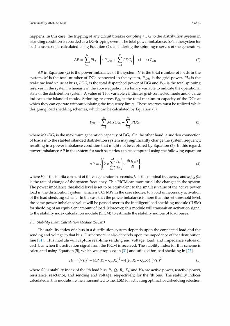
Loads were modeled as voltage- and frequency-dependent loads using the standard load modelin the PSCAD library. Classification of loads as non-critical, semi-critical, or critical was based on thetype of load, i.e., residential, industrial, municipal, and commercial. The loads and their rankings inthe system are shown in Table 1. Loads ranked 1 to 11 were assumed to be non-critical, loads ranked12 to 16 were classified as semi-critical, and the remaining four loads were ranked as critical, as seen inTable 1.
Sustainability 2020, 12, 6234 9 of 23
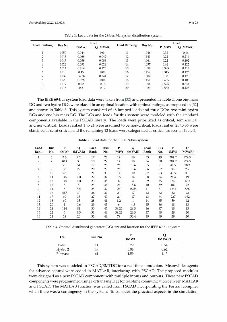
Table 1. Load data for the 28-bus Malaysian distribution system.
Load Ranking Bus No.Load Load Ranking Bus No.
LoadP (MW) Q (MVAR) P (MW) Q (MVAR)
1 1050 0.044 0.04 11 1046 0.32 0.162 1013 0.069 0.042 12 1141 0.22 0.2143 1047 0.059 0.088 13 1064 0.22 0.1924 1026 0.091 0.028 14 1057 0.46 0.1255 1012 0.314 0.125 15 1058 0.385 0.2136 1010 0.45 0.08 16 1154 0.315 0.1267 1039 0.4532 0.244 17 1004 0.33 0.1288 1020 0.078 0.06 18 1151 0.455 0.1069 1019 0.22 0.14 19 1056 0.595 0.34410 1018 0.2 0.12 20 1029 0.532 0.425
The IEEE 69-bus system load data were taken from [32] and presented in Table 2; one bio-massDG and two hydro DGs were placed in an optimal location with optimal ratings, as proposed in [32]and shown in Table 3. This system consisted of 48 lumped loads and three DGs: two mini-hydroDGs and one bio-mass DG. The DGs and loads for this system were modeled with the standardcomponents available in the PSCAD library. The loads were prioritized as critical, semi-critical,and non-critical. Loads ranked 1 to 24 were assumed to be non-critical, loads ranked 25 to 36 wereclassified as semi-critical, and the remaining 12 loads were categorized as critical, as seen in Table 2.
Table 2. Load data for the IEEE 69-bus system.
LoadRank
BusNo.
P(MW)
Q(MVAR)
LoadRank
BusNo.
P(MW)
Q(MVAR)
LoadRank
BusNo.
P(MW)
Q(MVAR)
1 6 2.6 2.2 17 26 14 10 33 49 384.7 274.52 7 40.4 30 18 27 14 10 34 50 384.7 274.53 8 75 54 19 28 26 18.6 35 51 40.5 28.34 9 30 22 20 29 26 18.6 36 52 3.6 2.75 10 28 19 21 33 14 10 37 53 4.35 3.56 11 145 104 22 34 9.5 14 38 54 26.4 197 12 145 104 23 35 6 4 39 55 24 17.28 13 8 5 24 36 26 18.6 40 59 100 729 14 8 5.5 25 37 26 18.55 41 61 1244 888
10 16 45.5 30 26 39 24 17 42 62 32 2311 17 60 35 27 40 24 17 43 64 227 16212 18 60 35 28 41 1.2 1 44 65 59 4213 20 1 0.6 29 43 6 4.3 45 66 18 1314 21 114 81 30 45 39.22 26.3 46 67 18 1315 22 5 3.5 31 46 39.22 26.3 47 68 28 2016 24 28 20 32 48 79 56.4 48 69 28 20
Table 3. Optimal distributed generator (DG) size and location for the IEEE 69-bus system.
DG Bus No. P(MW)
Q(MVAR)
Hydro 1 11 0.79 0.54Hydro 2 49 0.86 0.62Biomass 61 1.59 1.13
This system was modeled in PSCAD/EMTDC for a real-time simulation. Meanwhile, agentsfor advance control were coded in MATLAB, interfacing with PSCAD. The proposed moduleswere designed as a new PSCAD component with multiple inputs and outputs. These new PSCADcomponents were programmed using Fortran language for real-time communication between MATLABand PSCAD. The MATLAB function was called from PSCAD incorporating the Fortran compilerwhen there was a contingency in the system. To consider the practical aspects in the simulation,

Sustainability 2020, 12, 6234 10 of 23
circuit breaker operation time and communication delay between grid operation and load center wereassumed to be 100 ms, as in [9]. It was assumed that the remote circuit breaker operation facility andreal-time measurements were ensured for all the connected loads. Simulation was carried out with atime step of 250 uS on PSCAD (4.5.3) educational version interfaced with MATLAB R2014a, installedon a Core i5, 9th generation laptop.
Conventional and Adaptive Technique Modeling
The performance of the proposed scheme was compared with conventional and two adaptivetechniques. The conventional technique relied on under-frequency load shedding relay settings.Pre-defined load values were shed one by one for each threshold level of frequency. In this paper,an eight-step conventional load shedding utilized in [28] was resimulated to compare the results.On the other hand, the adaptive technique based on random and fixed priority loads (Adaptive-I)was resimulated in PSCAD/EMTDC by measuring the power imbalance of the system using swingequation and, subsequently, combinations of loads to be shed were selected using an exhaustive search,as in [28]. Loads were prioritized as random and fixed priority loads. The proposed method in theAdaptive-I technique found a combination of loads from random priority loads using an exhaustivesearch. If the power imbalance was higher than the sum of all random priority loads, it would shed allrandom priority loads and sequentially shed the fixed priority loads until the load shed amount wasequal to or greater than the power imbalance. Another adaptive load shedding technique based onthe voltage stability index (Adaptive-II) was also resimulated in PSCAD, which was proposed in [27].The voltage stability index was calculated and loads were arranged in ascending order with respectto stability. More unstable loads were shed sequentially until the load shed amount was equal to orgreater than the estimated power imbalance.
4. Results
Validation of the proposed technique was done by comparing the results of the proposedtechnique with the results obtained by the conventional and adaptive load shedding schemes.The proposed scheme was tested for different events: islanding, overloading, and DG tripping, withthree different scenarios.
• Scenario I: Islanding and DG-tripping events were simulated in this scenario for the 28-bus systemto compare the system frequency response (SFR) of the proposed technique with two adaptivetechniques, one based on an exhaustive search tool [28] to locate an optimal combination of loadsand other based on stability index calculation [27] to disconnect unstable loads on priority.
• Scenario II: An overloading event was simulated in an islanded system for the 28-bus system tocompare the SFR for conventional, Adaptive-I, Adaptive-II, and proposed techniques to validatethe effectiveness.
• Scenario III: Islanding and DG-tripping events were simulated in this scenario for the IEEE 69-bussystem to compare the SFR of the proposed technique with both adaptive techniques presentedin [27,28].
4.1. Scenario I
In this scenario, the proposed technique based on load priority and stability index was comparedwith the conventional and both adaptive techniques to validate the efficacy. Thirteen loads from thesystem were selected to form eight load groups (shown in Table 4) and were used for load sheddingin the Adaptive-I technique presented in [28]. The Adaptive-I technique was also simulated in thisscenario with all the system loads to test the effect of increasing the number of loads on the methodologyin [28].
Sustainability 2020, 12, 6234 11 of 23
Table 4. Load data for the adaptive technique.
Loads Ranked Bus No. P(MW)
a 1050 0.044b 1013 0.069c 1047,1026 0.15d 1012 0.314e 1010,1039 0.903f 1020, 1019, 1018, 1046 0.818g 1141 0.22h 1064 0.22
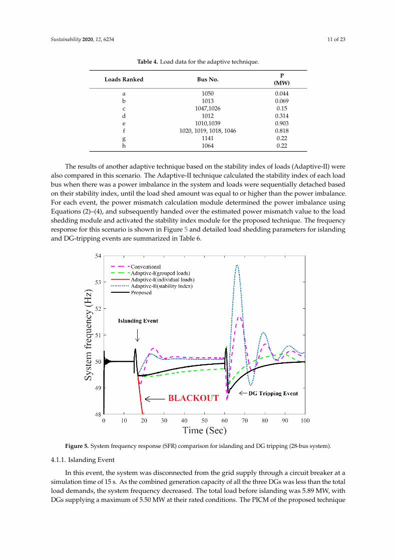
The results of another adaptive technique based on the stability index of loads (Adaptive-II) werealso compared in this scenario. The Adaptive-II technique calculated the stability index of each loadbus when there was a power imbalance in the system and loads were sequentially detached basedon their stability index, until the load shed amount was equal to or higher than the power imbalance.For each event, the power mismatch calculation module determined the power imbalance usingEquations (2)–(4), and subsequently handed over the estimated power mismatch value to the loadshedding module and activated the stability index module for the proposed technique. The frequencyresponse for this scenario is shown in Figure 5 and detailed load shedding parameters for islandingand DG-tripping events are summarized in Table 6.Sustainability 2020, 12, x FOR PEER REVIEW 11 of 23
Sustainability 2020, 12, x; doi: FOR PEER REVIEW www.mdpi.com/journal/sustainability
Figure 5. System frequency response (SFR) comparison for islanding and DG tripping (28-bus
system).
4.1.1. Islanding Event
In this event, the system was disconnected from the grid supply through a circuit breaker at a
simulation time of 15 s. As the combined generation capacity of all the three DGs was less than the
total load demands, the system frequency decreased. The total load before islanding was 5.89 MW,
with DGs supplying a maximum of 5.50 MW at their rated conditions. The PICM of the proposed
technique estimated a power imbalance of 0.39 MW in the system. The ILSM then captured and
processed this power mismatch to determine the best combination of loads to be shed.
It can be observed from Figure 5 that the conventional technique shed loads ranked 1–5 and
resulted in a significant overshoot of 50.7 Hz and a lower undershoot in the system frequency. This
was due to the extra amount of loads being shed and the multistage load shedding, respectively. The
results of the proposed method indicated a smoother frequency response without any overshoot and
disconnected an optimal combination of the more unstable loads ranked 2 and 11, which exactly
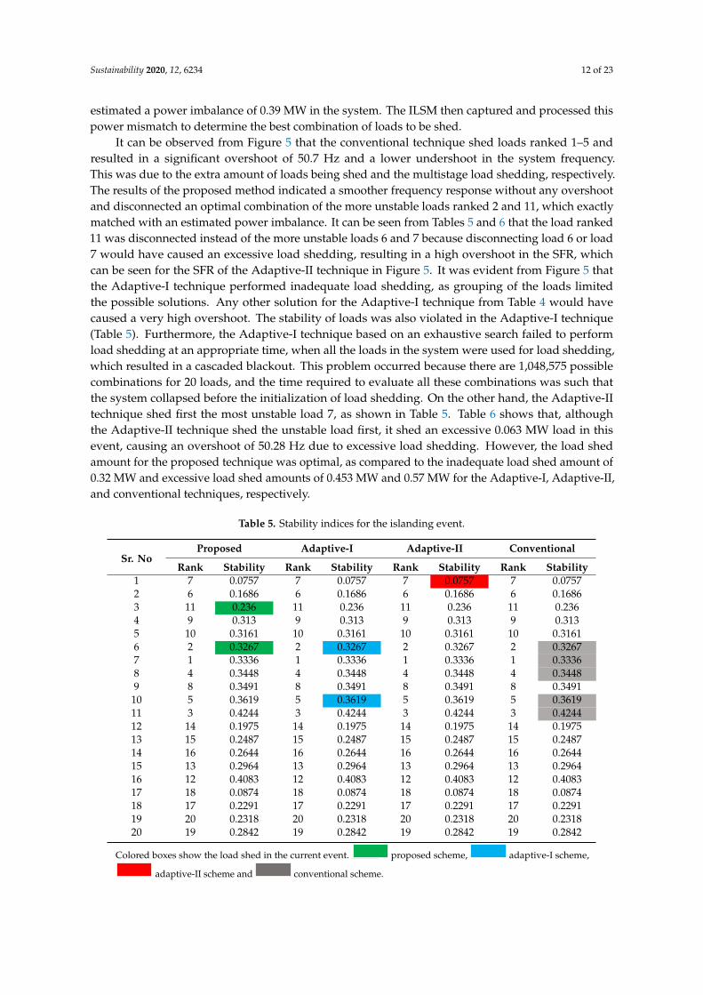
matched with an estimated power imbalance. It can be seen from Tables 5 and 6 that the load ranked
11 was disconnected instead of the more unstable loads 6 and 7 because disconnecting load 6 or load
7 would have caused an excessive load shedding, resulting in a high overshoot in the SFR, which can
be seen for the SFR of the Adaptive-II technique in Figure 5. It was evident from Figure 5 that the
Adaptive-I technique performed inadequate load shedding, as grouping of the loads limited the
possible solutions. Any other solution for the Adaptive-I technique from Table 4 would have caused
a very high overshoot. The stability of loads was also violated in the Adaptive-I technique (Table 5).
Furthermore, the Adaptive-I technique based on an exhaustive search failed to perform load
shedding at an appropriate time, when all the loads in the system were used for load shedding, which
resulted in a cascaded blackout. This problem occurred because there are 1,048,575 possible
combinations for 20 loads, and the time required to evaluate all these combinations was such that the
system collapsed before the initialization of load shedding. On the other hand, the Adaptive-II
technique shed first the most unstable load 7, as shown in Table 5. Table 6 shows that, although the
Adaptive-II technique shed the unstable load first, it shed an excessive 0.063 MW load in this event,
causing an overshoot of 50.28 Hz due to excessive load shedding. However, the load shed amount
for the proposed technique was optimal, as compared to the inadequate load shed amount of 0.32
Figure 5. System frequency response (SFR) comparison for islanding and DG tripping (28-bus system).
4.1.1. Islanding Event
In this event, the system was disconnected from the grid supply through a circuit breaker at asimulation time of 15 s. As the combined generation capacity of all the three DGs was less than the totalload demands, the system frequency decreased. The total load before islanding was 5.89 MW, withDGs supplying a maximum of 5.50 MW at their rated conditions. The PICM of the proposed technique
Sustainability 2020, 12, 6234 12 of 23
estimated a power imbalance of 0.39 MW in the system. The ILSM then captured and processed thispower mismatch to determine the best combination of loads to be shed.
It can be observed from Figure 5 that the conventional technique shed loads ranked 1–5 andresulted in a significant overshoot of 50.7 Hz and a lower undershoot in the system frequency.This was due to the extra amount of loads being shed and the multistage load shedding, respectively.The results of the proposed method indicated a smoother frequency response without any overshootand disconnected an optimal combination of the more unstable loads ranked 2 and 11, which exactlymatched with an estimated power imbalance. It can be seen from Tables 5 and 6 that the load ranked11 was disconnected instead of the more unstable loads 6 and 7 because disconnecting load 6 or load7 would have caused an excessive load shedding, resulting in a high overshoot in the SFR, whichcan be seen for the SFR of the Adaptive-II technique in Figure 5. It was evident from Figure 5 thatthe Adaptive-I technique performed inadequate load shedding, as grouping of the loads limitedthe possible solutions. Any other solution for the Adaptive-I technique from Table 4 would havecaused a very high overshoot. The stability of loads was also violated in the Adaptive-I technique(Table 5). Furthermore, the Adaptive-I technique based on an exhaustive search failed to performload shedding at an appropriate time, when all the loads in the system were used for load shedding,which resulted in a cascaded blackout. This problem occurred because there are 1,048,575 possiblecombinations for 20 loads, and the time required to evaluate all these combinations was such thatthe system collapsed before the initialization of load shedding. On the other hand, the Adaptive-IItechnique shed first the most unstable load 7, as shown in Table 5. Table 6 shows that, althoughthe Adaptive-II technique shed the unstable load first, it shed an excessive 0.063 MW load in thisevent, causing an overshoot of 50.28 Hz due to excessive load shedding. However, the load shedamount for the proposed technique was optimal, as compared to the inadequate load shed amount of0.32 MW and excessive load shed amounts of 0.453 MW and 0.57 MW for the Adaptive-I, Adaptive-II,and conventional techniques, respectively.
Table 5. Stability indices for the islanding event.
Sr. NoProposed Adaptive-I Adaptive-II Conventional
Rank Stability Rank Stability Rank Stability Rank Stability1 7 0.0757 7 0.0757 7 0.0757 7 0.07572 6 0.1686 6 0.1686 6 0.1686 6 0.16863 11 0.236 11 0.236 11 0.236 11 0.2364 9 0.313 9 0.313 9 0.313 9 0.3135 10 0.3161 10 0.3161 10 0.3161 10 0.31616 2 0.3267 2 0.3267 2 0.3267 2 0.32677 1 0.3336 1 0.3336 1 0.3336 1 0.33368 4 0.3448 4 0.3448 4 0.3448 4 0.34489 8 0.3491 8 0.3491 8 0.3491 8 0.3491
10 5 0.3619 5 0.3619 5 0.3619 5 0.361911 3 0.4244 3 0.4244 3 0.4244 3 0.424412 14 0.1975 14 0.1975 14 0.1975 14 0.197513 15 0.2487 15 0.2487 15 0.2487 15 0.248714 16 0.2644 16 0.2644 16 0.2644 16 0.264415 13 0.2964 13 0.2964 13 0.2964 13 0.296416 12 0.4083 12 0.4083 12 0.4083 12 0.408317 18 0.0874 18 0.0874 18 0.0874 18 0.087418 17 0.2291 17 0.2291 17 0.2291 17 0.229119 20 0.2318 20 0.2318 20 0.2318 20 0.231820 19 0.2842 19 0.2842 19 0.2842 19 0.2842
Colored boxes show the load shed in the current event.
Sustainability 2020, 12, x FOR PEER REVIEW 12 of 23
Sustainability 2020, 12, x; doi: FOR PEER REVIEW www.mdpi.com/journal/sustainability
MW and excessive load shed amounts of 0.453 MW and 0.57 MW for the Adaptive-I, Adaptive-II,
and conventional techniques, respectively.
Table 5. Stability indices for the islanding event.
Sr. No Proposed Adaptive-I Adaptive-II Conventional
Rank Stability Rank Stability Rank Stability Rank Stability
1 7 0.0757 7 0.0757 7 0.0757 7 0.0757
2 6 0.1686 6 0.1686 6 0.1686 6 0.1686
3 11 0.236 11 0.236 11 0.236 11 0.236
4 9 0.313 9 0.313 9 0.313 9 0.313
5 10 0.3161 10 0.3161 10 0.3161 10 0.3161
6 2 0.3267 2 0.3267 2 0.3267 2 0.3267
7 1 0.3336 1 0.3336 1 0.3336 1 0.3336
8 4 0.3448 4 0.3448 4 0.3448 4 0.3448
9 8 0.3491 8 0.3491 8 0.3491 8 0.3491
10 5 0.3619 5 0.3619 5 0.3619 5 0.3619
11 3 0.4244 3 0.4244 3 0.4244 3 0.4244
12 14 0.1975 14 0.1975 14 0.1975 14 0.1975
13 15 0.2487 15 0.2487 15 0.2487 15 0.2487
14 16 0.2644 16 0.2644 16 0.2644 16 0.2644
15 13 0.2964 13 0.2964 13 0.2964 13 0.2964
16 12 0.4083 12 0.4083 12 0.4083 12 0.4083
17 18 0.0874 18 0.0874 18 0.0874 18 0.0874
18 17 0.2291 17 0.2291 17 0.2291 17 0.2291
19 20 0.2318 20 0.2318 20 0.2318 20 0.2318
20 19 0.2842 19 0.2842 19 0.2842 19 0.2842
Colored boxes show the load shed in the current event. proposed scheme, adaptive-I
scheme, adaptive-II scheme and conventional scheme
Table 6. Frequency stability parameters for comparison (Scenario I).
Parameters Islanding Event DG-Tripping Event
Prop Adap-I Adap-II Conv Prop Adap-I Adap-II Conv
Power imbalance (MW) 0.39 0.39 0.39 0.39 1.891 1.891 1.891 1.89
Load shed amount (MW) 0.38 0.32 0.453 0.57 1.890 2.071 2.304 2.127
Excessive load shed (MW) −0.001 −0.007 0.063 0.18 −0.001 0.18 0.414 0.237
Loads switched off 2, 11 b, d 7 1–5 1, 4, 5, 6, 7, 10, 15 a–g 1–11,14 1–13
Frequency undershoot (Hz) 49.453 49.452 49.48 49.1 48.8 49 48.86 48.54
Frequency overshoot (Hz) - - 50.28 50.5 - 50.28 53.6 51.7
4.1.2. DG Tripping in an Islanded System
For validation of the proposed method, one of the DGs was disconnected from the system during
the islanded mode. The bio-mass DG was disconnected at time t = 60 s when the system was operating
in islanded mode. Figure 5 shows the frequency response of the system, and frequency stability
parameters are compared in Table 6. The conventional technique shed loads ranked 6–13 in addition
to loads shed in Scenario 1, resulting in a frequency overshoot of 51.7 Hz. Loads ranked ‘a’ to ‘g’ in
Table 4 were shed for the Adaptive-I technique. It is visible from Figure 5 that frequency was stabled
for the proposed technique without any overshoot, as compared to an overshoot of 50.28 Hz, 53.6
HZ, and 51.7 Hz for the Adaptive-I, Adaptive-II, and conventional techniques, respectively.
The overshoot in the SFR for the Adaptive-I technique was due to the fact that the power
imbalance was higher than the total random priority loads, and a fixed priority load was
disconnected in addition to all random priority loads. Therefore, an additional 0.18 MW load was
shed for the Adaptive-I technique, as can be seen in Table 6. However, the Adaptive-II technique
proposed scheme,
Sustainability 2020, 12, x FOR PEER REVIEW 12 of 23
Sustainability 2020, 12, x; doi: FOR PEER REVIEW www.mdpi.com/journal/sustainability
MW and excessive load shed amounts of 0.453 MW and 0.57 MW for the Adaptive-I, Adaptive-II,
and conventional techniques, respectively.
Table 5. Stability indices for the islanding event.
Sr. No Proposed Adaptive-I Adaptive-II Conventional
Rank Stability Rank Stability Rank Stability Rank Stability
1 7 0.0757 7 0.0757 7 0.0757 7 0.0757
2 6 0.1686 6 0.1686 6 0.1686 6 0.1686
3 11 0.236 11 0.236 11 0.236 11 0.236
4 9 0.313 9 0.313 9 0.313 9 0.313
5 10 0.3161 10 0.3161 10 0.3161 10 0.3161
6 2 0.3267 2 0.3267 2 0.3267 2 0.3267
7 1 0.3336 1 0.3336 1 0.3336 1 0.3336
8 4 0.3448 4 0.3448 4 0.3448 4 0.3448
9 8 0.3491 8 0.3491 8 0.3491 8 0.3491
10 5 0.3619 5 0.3619 5 0.3619 5 0.3619
11 3 0.4244 3 0.4244 3 0.4244 3 0.4244
12 14 0.1975 14 0.1975 14 0.1975 14 0.1975
13 15 0.2487 15 0.2487 15 0.2487 15 0.2487
14 16 0.2644 16 0.2644 16 0.2644 16 0.2644
15 13 0.2964 13 0.2964 13 0.2964 13 0.2964
16 12 0.4083 12 0.4083 12 0.4083 12 0.4083
17 18 0.0874 18 0.0874 18 0.0874 18 0.0874
18 17 0.2291 17 0.2291 17 0.2291 17 0.2291
19 20 0.2318 20 0.2318 20 0.2318 20 0.2318
20 19 0.2842 19 0.2842 19 0.2842 19 0.2842
Colored boxes show the load shed in the current event. proposed scheme, adaptive-I
scheme, adaptive-II scheme and conventional scheme
Table 6. Frequency stability parameters for comparison (Scenario I).
Parameters Islanding Event DG-Tripping Event
Prop Adap-I Adap-II Conv Prop Adap-I Adap-II Conv
Power imbalance (MW) 0.39 0.39 0.39 0.39 1.891 1.891 1.891 1.89
Load shed amount (MW) 0.38 0.32 0.453 0.57 1.890 2.071 2.304 2.127
Excessive load shed (MW) −0.001 −0.007 0.063 0.18 −0.001 0.18 0.414 0.237
Loads switched off 2, 11 b, d 7 1–5 1, 4, 5, 6, 7, 10, 15 a–g 1–11,14 1–13
Frequency undershoot (Hz) 49.453 49.452 49.48 49.1 48.8 49 48.86 48.54
Frequency overshoot (Hz) - - 50.28 50.5 - 50.28 53.6 51.7
4.1.2. DG Tripping in an Islanded System
For validation of the proposed method, one of the DGs was disconnected from the system during
the islanded mode. The bio-mass DG was disconnected at time t = 60 s when the system was operating
in islanded mode. Figure 5 shows the frequency response of the system, and frequency stability
parameters are compared in Table 6. The conventional technique shed loads ranked 6–13 in addition
to loads shed in Scenario 1, resulting in a frequency overshoot of 51.7 Hz. Loads ranked ‘a’ to ‘g’ in
Table 4 were shed for the Adaptive-I technique. It is visible from Figure 5 that frequency was stabled
for the proposed technique without any overshoot, as compared to an overshoot of 50.28 Hz, 53.6
HZ, and 51.7 Hz for the Adaptive-I, Adaptive-II, and conventional techniques, respectively.
The overshoot in the SFR for the Adaptive-I technique was due to the fact that the power
imbalance was higher than the total random priority loads, and a fixed priority load was
disconnected in addition to all random priority loads. Therefore, an additional 0.18 MW load was
shed for the Adaptive-I technique, as can be seen in Table 6. However, the Adaptive-II technique
adaptive-I scheme,
Sustainability 2020, 12, x FOR PEER REVIEW 13 of 23
Sustainability 2020, 12, x; doi: FOR PEER REVIEW www.mdpi.com/journal/sustainability
shed more unstable non-critical loads sequentially, as seen in Table 7, to match with an estimated
power imbalance. The power imbalance for this event was higher than the total non-critical loads,
therefore the Adaptive-II technique shed the most unstable load from the semi-critical loads, which
was ranked 15. This resulted in an excessive load shed amount of 0.414 MW, causing a huge
overshoot of 53.6 Hz in the SFR, whereas the proposed technique disconnected more unstable non-
critical loads on priority and found an optimal combination of one semi-critical and six non-critical
loads for this event. Table 7 shows that the proposed scheme selected unstable loads to match with
the estimated power imbalance. It can be estimated from Table 6 that the load retained in the system
was 5.72%, 11.5%, and 6.58% higher than the Adaptive-I, Adaptive-II, and conventional techniques,
respectively. Therefore, the SFR in Figure 5 proves that the optimal amount of load was shed for the
proposed technique and the frequency response was smoother and more accurate than the
conventional and adaptive techniques.
Table 7. Stability index of load buses for DG-tripping event.
Sr. No Proposed Adaptive-I Adaptive-II Conventional
Rank Stability Rank Stability Rank Stability Rank Stability
1 2 - 2 - 7 - 1 -
2 11 - 5 - 6 0.1667 2 -
3 7 0.0749 7 0.0749 11 0.2393 4 -
4 6 0.1667 6 0.1667 9 0.3186 5 -
5 9 0.3186 11 0.2393 1 0.3206 3 -
6 1 0.3206 9 0.3186 10 0.3214 7 0.0749
7 10 0.3214 1 0.3206 2 0.3395 6 0.1667
8 4 0.3488 10 0.3214 4 0.3488 11 0.2393
9 8 0.3555 4 0.3488 8 0.3555 9 0.3186
10 5 0.3783 8 0.3555 5 0.3783 10 0.3214
11 3 0.4287 3 0.4287 3 0.4287 8 0.3555
12 14 0.1894 14 0.1894 14 0.1894 14 0.1894
13 15 0.2465 15 0.2465 15 0.2465 15 0.2465
14 16 0.2504 16 0.2504 16 0.2504 16 0.2504
15 13 0.2906 13 0.2906 13 0.2906 13 0.2906
16 12 0.4234 12 0.4234 12 0.4234 12 0.4234
17 18 0.0851 18 0.0851 18 0.0851 18 0.0851
18 20 0.2225 20 0.2225 20 0.2225 20 0.2225
19 17 0.2404 17 0.2404 17 0.2404 17 0.2404
20 19 0.285 19 0.285 19 0.285 19 0.285
Colored boxes show the load shed in the current event. proposed scheme, adaptive-I
scheme, adaptive-II scheme and conventional scheme
It can be concluded from this scenario that, although the Adaptive-I technique based on an
exhaustive search produced accurate results, its application, however, was quite limited. An increase
in n number of loads exponentially increased the possible load combination to 2n. It became an
infeasible approach to load shedding as the memory space required to store and evaluate 2n
combinations became unreal. Moreover, the time taken to find a solution also increased with the
number of loads, which would have triggered the operation of protective relays, resulting in a
blackout before the load shedding could take place. It is clear from the results in this scenario that the
Adaptive-II technique shed more unstable loads on priority to avoid any operation of undervoltage
protection; the frequency of the system was assumed to be stabilized in [29]. However, the SFR in
Figure 5 clearly reveals that optimal load shedding was needed to avoid overshoot in the system
frequency.
4.2. Scenario II
The practical load of an islanded system is usually variable. This variation in load causes
instability in system frequency. The total load in the system may increase due to the additional load
adaptive-II scheme and
Sustainability 2020, 12, x FOR PEER REVIEW 13 of 23
Sustainability 2020, 12, x; doi: FOR PEER REVIEW www.mdpi.com/journal/sustainability
shed more unstable non-critical loads sequentially, as seen in Table 7, to match with an estimated
power imbalance. The power imbalance for this event was higher than the total non-critical loads,
therefore the Adaptive-II technique shed the most unstable load from the semi-critical loads, which
was ranked 15. This resulted in an excessive load shed amount of 0.414 MW, causing a huge
overshoot of 53.6 Hz in the SFR, whereas the proposed technique disconnected more unstable non-
critical loads on priority and found an optimal combination of one semi-critical and six non-critical
loads for this event. Table 7 shows that the proposed scheme selected unstable loads to match with
the estimated power imbalance. It can be estimated from Table 6 that the load retained in the system
was 5.72%, 11.5%, and 6.58% higher than the Adaptive-I, Adaptive-II, and conventional techniques,
respectively. Therefore, the SFR in Figure 5 proves that the optimal amount of load was shed for the
proposed technique and the frequency response was smoother and more accurate than the
conventional and adaptive techniques.
Table 7. Stability index of load buses for DG-tripping event.
Sr. No Proposed Adaptive-I Adaptive-II Conventional
Rank Stability Rank Stability Rank Stability Rank Stability
1 2 - 2 - 7 - 1 -
2 11 - 5 - 6 0.1667 2 -
3 7 0.0749 7 0.0749 11 0.2393 4 -
4 6 0.1667 6 0.1667 9 0.3186 5 -
5 9 0.3186 11 0.2393 1 0.3206 3 -
6 1 0.3206 9 0.3186 10 0.3214 7 0.0749
7 10 0.3214 1 0.3206 2 0.3395 6 0.1667
8 4 0.3488 10 0.3214 4 0.3488 11 0.2393
9 8 0.3555 4 0.3488 8 0.3555 9 0.3186
10 5 0.3783 8 0.3555 5 0.3783 10 0.3214
11 3 0.4287 3 0.4287 3 0.4287 8 0.3555
12 14 0.1894 14 0.1894 14 0.1894 14 0.1894
13 15 0.2465 15 0.2465 15 0.2465 15 0.2465
14 16 0.2504 16 0.2504 16 0.2504 16 0.2504
15 13 0.2906 13 0.2906 13 0.2906 13 0.2906
16 12 0.4234 12 0.4234 12 0.4234 12 0.4234
17 18 0.0851 18 0.0851 18 0.0851 18 0.0851
18 20 0.2225 20 0.2225 20 0.2225 20 0.2225
19 17 0.2404 17 0.2404 17 0.2404 17 0.2404
20 19 0.285 19 0.285 19 0.285 19 0.285
Colored boxes show the load shed in the current event. proposed scheme, adaptive-I
scheme, adaptive-II scheme and conventional scheme
It can be concluded from this scenario that, although the Adaptive-I technique based on an
exhaustive search produced accurate results, its application, however, was quite limited. An increase
in n number of loads exponentially increased the possible load combination to 2n. It became an
infeasible approach to load shedding as the memory space required to store and evaluate 2n
combinations became unreal. Moreover, the time taken to find a solution also increased with the
number of loads, which would have triggered the operation of protective relays, resulting in a
blackout before the load shedding could take place. It is clear from the results in this scenario that the
Adaptive-II technique shed more unstable loads on priority to avoid any operation of undervoltage
protection; the frequency of the system was assumed to be stabilized in [29]. However, the SFR in
Figure 5 clearly reveals that optimal load shedding was needed to avoid overshoot in the system
frequency.
4.2. Scenario II
The practical load of an islanded system is usually variable. This variation in load causes
instability in system frequency. The total load in the system may increase due to the additional load
conventional scheme.

Sustainability 2020, 12, 6234 13 of 23
Table 6. Frequency stability parameters for comparison (Scenario I).
ParametersIslanding Event DG-Tripping Event
Prop Adap-I Adap-II Conv Prop Adap-I Adap-II Conv
Power imbalance (MW) 0.39 0.39 0.39 0.39 1.891 1.891 1.891 1.89Load shed amount (MW) 0.38 0.32 0.453 0.57 1.890 2.071 2.304 2.127Excessive load shed (MW) −0.001 −0.007 0.063 0.18 −0.001 0.18 0.414 0.237
Loads switched off 2, 11 b, d 7 1–5 1, 4, 5, 6, 7, 10, 15 a–g 1–11,14 1–13Frequency undershoot (Hz) 49.453 49.452 49.48 49.1 48.8 49 48.86 48.54Frequency overshoot (Hz) - - 50.28 50.5 - 50.28 53.6 51.7
4.1.2. DG Tripping in an Islanded System
For validation of the proposed method, one of the DGs was disconnected from the system duringthe islanded mode. The bio-mass DG was disconnected at time t = 60 s when the system was operatingin islanded mode. Figure 5 shows the frequency response of the system, and frequency stabilityparameters are compared in Table 6. The conventional technique shed loads ranked 6–13 in additionto loads shed in Scenario 1, resulting in a frequency overshoot of 51.7 Hz. Loads ranked ‘a’ to ‘g’ inTable 4 were shed for the Adaptive-I technique. It is visible from Figure 5 that frequency was stabledfor the proposed technique without any overshoot, as compared to an overshoot of 50.28 Hz, 53.6 HZ,and 51.7 Hz for the Adaptive-I, Adaptive-II, and conventional techniques, respectively.
The overshoot in the SFR for the Adaptive-I technique was due to the fact that the powerimbalance was higher than the total random priority loads, and a fixed priority load was disconnectedin addition to all random priority loads. Therefore, an additional 0.18 MW load was shed for theAdaptive-I technique, as can be seen in Table 6. However, the Adaptive-II technique shed moreunstable non-critical loads sequentially, as seen in Table 7, to match with an estimated power imbalance.The power imbalance for this event was higher than the total non-critical loads, therefore the Adaptive-IItechnique shed the most unstable load from the semi-critical loads, which was ranked 15. This resultedin an excessive load shed amount of 0.414 MW, causing a huge overshoot of 53.6 Hz in the SFR,whereas the proposed technique disconnected more unstable non-critical loads on priority and foundan optimal combination of one semi-critical and six non-critical loads for this event. Table 7 shows thatthe proposed scheme selected unstable loads to match with the estimated power imbalance. It canbe estimated from Table 6 that the load retained in the system was 5.72%, 11.5%, and 6.58% higherthan the Adaptive-I, Adaptive-II, and conventional techniques, respectively. Therefore, the SFR inFigure 5 proves that the optimal amount of load was shed for the proposed technique and the frequencyresponse was smoother and more accurate than the conventional and adaptive techniques.
It can be concluded from this scenario that, although the Adaptive-I technique based on anexhaustive search produced accurate results, its application, however, was quite limited. An increase inn number of loads exponentially increased the possible load combination to 2n. It became an infeasibleapproach to load shedding as the memory space required to store and evaluate 2n combinationsbecame unreal. Moreover, the time taken to find a solution also increased with the number of loads,which would have triggered the operation of protective relays, resulting in a blackout before the loadshedding could take place. It is clear from the results in this scenario that the Adaptive-II techniqueshed more unstable loads on priority to avoid any operation of undervoltage protection; the frequencyof the system was assumed to be stabilized in [29]. However, the SFR in Figure 5 clearly reveals thatoptimal load shedding was needed to avoid overshoot in the system frequency.

Sustainability 2020, 12, 6234 14 of 23
Table 7. Stability index of load buses for DG-tripping event.
Sr. NoProposed Adaptive-I Adaptive-II Conventional
Rank Stability Rank Stability Rank Stability Rank Stability1 2 - 2 - 7 - 1 -2 11 - 5 - 6 0.1667 2 -3 7 0.0749 7 0.0749 11 0.2393 4 -4 6 0.1667 6 0.1667 9 0.3186 5 -5 9 0.3186 11 0.2393 1 0.3206 3 -6 1 0.3206 9 0.3186 10 0.3214 7 0.07497 10 0.3214 1 0.3206 2 0.3395 6 0.16678 4 0.3488 10 0.3214 4 0.3488 11 0.23939 8 0.3555 4 0.3488 8 0.3555 9 0.3186
10 5 0.3783 8 0.3555 5 0.3783 10 0.321411 3 0.4287 3 0.4287 3 0.4287 8 0.355512 14 0.1894 14 0.1894 14 0.1894 14 0.189413 15 0.2465 15 0.2465 15 0.2465 15 0.246514 16 0.2504 16 0.2504 16 0.2504 16 0.250415 13 0.2906 13 0.2906 13 0.2906 13 0.290616 12 0.4234 12 0.4234 12 0.4234 12 0.423417 18 0.0851 18 0.0851 18 0.0851 18 0.085118 20 0.2225 20 0.2225 20 0.2225 20 0.222519 17 0.2404 17 0.2404 17 0.2404 17 0.240420 19 0.285 19 0.285 19 0.285 19 0.285
Colored boxes show the load shed in the current event.
Sustainability 2020, 12, x FOR PEER REVIEW 12 of 23
Sustainability 2020, 12, x; doi: FOR PEER REVIEW www.mdpi.com/journal/sustainability
MW and excessive load shed amounts of 0.453 MW and 0.57 MW for the Adaptive-I, Adaptive-II,
and conventional techniques, respectively.
Table 5. Stability indices for the islanding event.
Sr. No Proposed Adaptive-I Adaptive-II Conventional
Rank Stability Rank Stability Rank Stability Rank Stability
1 7 0.0757 7 0.0757 7 0.0757 7 0.0757
2 6 0.1686 6 0.1686 6 0.1686 6 0.1686
3 11 0.236 11 0.236 11 0.236 11 0.236
4 9 0.313 9 0.313 9 0.313 9 0.313
5 10 0.3161 10 0.3161 10 0.3161 10 0.3161
6 2 0.3267 2 0.3267 2 0.3267 2 0.3267
7 1 0.3336 1 0.3336 1 0.3336 1 0.3336
8 4 0.3448 4 0.3448 4 0.3448 4 0.3448
9 8 0.3491 8 0.3491 8 0.3491 8 0.3491
10 5 0.3619 5 0.3619 5 0.3619 5 0.3619
11 3 0.4244 3 0.4244 3 0.4244 3 0.4244
12 14 0.1975 14 0.1975 14 0.1975 14 0.1975
13 15 0.2487 15 0.2487 15 0.2487 15 0.2487
14 16 0.2644 16 0.2644 16 0.2644 16 0.2644
15 13 0.2964 13 0.2964 13 0.2964 13 0.2964
16 12 0.4083 12 0.4083 12 0.4083 12 0.4083
17 18 0.0874 18 0.0874 18 0.0874 18 0.0874
18 17 0.2291 17 0.2291 17 0.2291 17 0.2291
19 20 0.2318 20 0.2318 20 0.2318 20 0.2318
20 19 0.2842 19 0.2842 19 0.2842 19 0.2842
Colored boxes show the load shed in the current event. proposed scheme, adaptive-I
scheme, adaptive-II scheme and conventional scheme
Table 6. Frequency stability parameters for comparison (Scenario I).
Parameters Islanding Event DG-Tripping Event
Prop Adap-I Adap-II Conv Prop Adap-I Adap-II Conv
Power imbalance (MW) 0.39 0.39 0.39 0.39 1.891 1.891 1.891 1.89
Load shed amount (MW) 0.38 0.32 0.453 0.57 1.890 2.071 2.304 2.127
Excessive load shed (MW) −0.001 −0.007 0.063 0.18 −0.001 0.18 0.414 0.237
Loads switched off 2, 11 b, d 7 1–5 1, 4, 5, 6, 7, 10, 15 a–g 1–11,14 1–13
Frequency undershoot (Hz) 49.453 49.452 49.48 49.1 48.8 49 48.86 48.54
Frequency overshoot (Hz) - - 50.28 50.5 - 50.28 53.6 51.7
4.1.2. DG Tripping in an Islanded System
For validation of the proposed method, one of the DGs was disconnected from the system during
the islanded mode. The bio-mass DG was disconnected at time t = 60 s when the system was operating
in islanded mode. Figure 5 shows the frequency response of the system, and frequency stability
parameters are compared in Table 6. The conventional technique shed loads ranked 6–13 in addition
to loads shed in Scenario 1, resulting in a frequency overshoot of 51.7 Hz. Loads ranked ‘a’ to ‘g’ in
Table 4 were shed for the Adaptive-I technique. It is visible from Figure 5 that frequency was stabled
for the proposed technique without any overshoot, as compared to an overshoot of 50.28 Hz, 53.6
HZ, and 51.7 Hz for the Adaptive-I, Adaptive-II, and conventional techniques, respectively.
The overshoot in the SFR for the Adaptive-I technique was due to the fact that the power
imbalance was higher than the total random priority loads, and a fixed priority load was
disconnected in addition to all random priority loads. Therefore, an additional 0.18 MW load was
shed for the Adaptive-I technique, as can be seen in Table 6. However, the Adaptive-II technique
proposed scheme,
Sustainability 2020, 12, x FOR PEER REVIEW 12 of 23
Sustainability 2020, 12, x; doi: FOR PEER REVIEW www.mdpi.com/journal/sustainability
MW and excessive load shed amounts of 0.453 MW and 0.57 MW for the Adaptive-I, Adaptive-II,
and conventional techniques, respectively.
Table 5. Stability indices for the islanding event.
Sr. No Proposed Adaptive-I Adaptive-II Conventional
Rank Stability Rank Stability Rank Stability Rank Stability
1 7 0.0757 7 0.0757 7 0.0757 7 0.0757
2 6 0.1686 6 0.1686 6 0.1686 6 0.1686
3 11 0.236 11 0.236 11 0.236 11 0.236
4 9 0.313 9 0.313 9 0.313 9 0.313
5 10 0.3161 10 0.3161 10 0.3161 10 0.3161
6 2 0.3267 2 0.3267 2 0.3267 2 0.3267
7 1 0.3336 1 0.3336 1 0.3336 1 0.3336
8 4 0.3448 4 0.3448 4 0.3448 4 0.3448
9 8 0.3491 8 0.3491 8 0.3491 8 0.3491
10 5 0.3619 5 0.3619 5 0.3619 5 0.3619
11 3 0.4244 3 0.4244 3 0.4244 3 0.4244
12 14 0.1975 14 0.1975 14 0.1975 14 0.1975
13 15 0.2487 15 0.2487 15 0.2487 15 0.2487
14 16 0.2644 16 0.2644 16 0.2644 16 0.2644
15 13 0.2964 13 0.2964 13 0.2964 13 0.2964
16 12 0.4083 12 0.4083 12 0.4083 12 0.4083
17 18 0.0874 18 0.0874 18 0.0874 18 0.0874
18 17 0.2291 17 0.2291 17 0.2291 17 0.2291
19 20 0.2318 20 0.2318 20 0.2318 20 0.2318
20 19 0.2842 19 0.2842 19 0.2842 19 0.2842
Colored boxes show the load shed in the current event. proposed scheme, adaptive-I
scheme, adaptive-II scheme and conventional scheme
Table 6. Frequency stability parameters for comparison (Scenario I).
Parameters Islanding Event DG-Tripping Event
Prop Adap-I Adap-II Conv Prop Adap-I Adap-II Conv
Power imbalance (MW) 0.39 0.39 0.39 0.39 1.891 1.891 1.891 1.89
Load shed amount (MW) 0.38 0.32 0.453 0.57 1.890 2.071 2.304 2.127
Excessive load shed (MW) −0.001 −0.007 0.063 0.18 −0.001 0.18 0.414 0.237
Loads switched off 2, 11 b, d 7 1–5 1, 4, 5, 6, 7, 10, 15 a–g 1–11,14 1–13
Frequency undershoot (Hz) 49.453 49.452 49.48 49.1 48.8 49 48.86 48.54
Frequency overshoot (Hz) - - 50.28 50.5 - 50.28 53.6 51.7
4.1.2. DG Tripping in an Islanded System
For validation of the proposed method, one of the DGs was disconnected from the system during
the islanded mode. The bio-mass DG was disconnected at time t = 60 s when the system was operating
in islanded mode. Figure 5 shows the frequency response of the system, and frequency stability
parameters are compared in Table 6. The conventional technique shed loads ranked 6–13 in addition
to loads shed in Scenario 1, resulting in a frequency overshoot of 51.7 Hz. Loads ranked ‘a’ to ‘g’ in
Table 4 were shed for the Adaptive-I technique. It is visible from Figure 5 that frequency was stabled
for the proposed technique without any overshoot, as compared to an overshoot of 50.28 Hz, 53.6
HZ, and 51.7 Hz for the Adaptive-I, Adaptive-II, and conventional techniques, respectively.
The overshoot in the SFR for the Adaptive-I technique was due to the fact that the power
imbalance was higher than the total random priority loads, and a fixed priority load was
disconnected in addition to all random priority loads. Therefore, an additional 0.18 MW load was
shed for the Adaptive-I technique, as can be seen in Table 6. However, the Adaptive-II technique
adaptive-I scheme,
Sustainability 2020, 12, x FOR PEER REVIEW 13 of 23
Sustainability 2020, 12, x; doi: FOR PEER REVIEW www.mdpi.com/journal/sustainability
shed more unstable non-critical loads sequentially, as seen in Table 7, to match with an estimated
power imbalance. The power imbalance for this event was higher than the total non-critical loads,
therefore the Adaptive-II technique shed the most unstable load from the semi-critical loads, which
was ranked 15. This resulted in an excessive load shed amount of 0.414 MW, causing a huge
overshoot of 53.6 Hz in the SFR, whereas the proposed technique disconnected more unstable non-
critical loads on priority and found an optimal combination of one semi-critical and six non-critical
loads for this event. Table 7 shows that the proposed scheme selected unstable loads to match with
the estimated power imbalance. It can be estimated from Table 6 that the load retained in the system
was 5.72%, 11.5%, and 6.58% higher than the Adaptive-I, Adaptive-II, and conventional techniques,
respectively. Therefore, the SFR in Figure 5 proves that the optimal amount of load was shed for the
proposed technique and the frequency response was smoother and more accurate than the
conventional and adaptive techniques.
Table 7. Stability index of load buses for DG-tripping event.
Sr. No Proposed Adaptive-I Adaptive-II Conventional
Rank Stability Rank Stability Rank Stability Rank Stability
1 2 - 2 - 7 - 1 -
2 11 - 5 - 6 0.1667 2 -
3 7 0.0749 7 0.0749 11 0.2393 4 -
4 6 0.1667 6 0.1667 9 0.3186 5 -
5 9 0.3186 11 0.2393 1 0.3206 3 -
6 1 0.3206 9 0.3186 10 0.3214 7 0.0749
7 10 0.3214 1 0.3206 2 0.3395 6 0.1667
8 4 0.3488 10 0.3214 4 0.3488 11 0.2393
9 8 0.3555 4 0.3488 8 0.3555 9 0.3186
10 5 0.3783 8 0.3555 5 0.3783 10 0.3214
11 3 0.4287 3 0.4287 3 0.4287 8 0.3555
12 14 0.1894 14 0.1894 14 0.1894 14 0.1894
13 15 0.2465 15 0.2465 15 0.2465 15 0.2465
14 16 0.2504 16 0.2504 16 0.2504 16 0.2504
15 13 0.2906 13 0.2906 13 0.2906 13 0.2906
16 12 0.4234 12 0.4234 12 0.4234 12 0.4234
17 18 0.0851 18 0.0851 18 0.0851 18 0.0851
18 20 0.2225 20 0.2225 20 0.2225 20 0.2225
19 17 0.2404 17 0.2404 17 0.2404 17 0.2404
20 19 0.285 19 0.285 19 0.285 19 0.285
Colored boxes show the load shed in the current event. proposed scheme, adaptive-I
scheme, adaptive-II scheme and conventional scheme
It can be concluded from this scenario that, although the Adaptive-I technique based on an
exhaustive search produced accurate results, its application, however, was quite limited. An increase
in n number of loads exponentially increased the possible load combination to 2n. It became an
infeasible approach to load shedding as the memory space required to store and evaluate 2n
combinations became unreal. Moreover, the time taken to find a solution also increased with the
number of loads, which would have triggered the operation of protective relays, resulting in a
blackout before the load shedding could take place. It is clear from the results in this scenario that the
Adaptive-II technique shed more unstable loads on priority to avoid any operation of undervoltage
protection; the frequency of the system was assumed to be stabilized in [29]. However, the SFR in
Figure 5 clearly reveals that optimal load shedding was needed to avoid overshoot in the system
frequency.
4.2. Scenario II
The practical load of an islanded system is usually variable. This variation in load causes
instability in system frequency. The total load in the system may increase due to the additional load
adaptive-II scheme and
Sustainability 2020, 12, x FOR PEER REVIEW 13 of 23
Sustainability 2020, 12, x; doi: FOR PEER REVIEW www.mdpi.com/journal/sustainability
shed more unstable non-critical loads sequentially, as seen in Table 7, to match with an estimated
power imbalance. The power imbalance for this event was higher than the total non-critical loads,
therefore the Adaptive-II technique shed the most unstable load from the semi-critical loads, which
was ranked 15. This resulted in an excessive load shed amount of 0.414 MW, causing a huge
overshoot of 53.6 Hz in the SFR, whereas the proposed technique disconnected more unstable non-
critical loads on priority and found an optimal combination of one semi-critical and six non-critical
loads for this event. Table 7 shows that the proposed scheme selected unstable loads to match with
the estimated power imbalance. It can be estimated from Table 6 that the load retained in the system
was 5.72%, 11.5%, and 6.58% higher than the Adaptive-I, Adaptive-II, and conventional techniques,
respectively. Therefore, the SFR in Figure 5 proves that the optimal amount of load was shed for the
proposed technique and the frequency response was smoother and more accurate than the
conventional and adaptive techniques.
Table 7. Stability index of load buses for DG-tripping event.
Sr. No Proposed Adaptive-I Adaptive-II Conventional
Rank Stability Rank Stability Rank Stability Rank Stability
1 2 - 2 - 7 - 1 -
2 11 - 5 - 6 0.1667 2 -
3 7 0.0749 7 0.0749 11 0.2393 4 -
4 6 0.1667 6 0.1667 9 0.3186 5 -
5 9 0.3186 11 0.2393 1 0.3206 3 -
6 1 0.3206 9 0.3186 10 0.3214 7 0.0749
7 10 0.3214 1 0.3206 2 0.3395 6 0.1667
8 4 0.3488 10 0.3214 4 0.3488 11 0.2393
9 8 0.3555 4 0.3488 8 0.3555 9 0.3186
10 5 0.3783 8 0.3555 5 0.3783 10 0.3214
11 3 0.4287 3 0.4287 3 0.4287 8 0.3555
12 14 0.1894 14 0.1894 14 0.1894 14 0.1894
13 15 0.2465 15 0.2465 15 0.2465 15 0.2465
14 16 0.2504 16 0.2504 16 0.2504 16 0.2504
15 13 0.2906 13 0.2906 13 0.2906 13 0.2906
16 12 0.4234 12 0.4234 12 0.4234 12 0.4234
17 18 0.0851 18 0.0851 18 0.0851 18 0.0851
18 20 0.2225 20 0.2225 20 0.2225 20 0.2225
19 17 0.2404 17 0.2404 17 0.2404 17 0.2404
20 19 0.285 19 0.285 19 0.285 19 0.285
Colored boxes show the load shed in the current event. proposed scheme, adaptive-I
scheme, adaptive-II scheme and conventional scheme
It can be concluded from this scenario that, although the Adaptive-I technique based on an
exhaustive search produced accurate results, its application, however, was quite limited. An increase
in n number of loads exponentially increased the possible load combination to 2n. It became an
infeasible approach to load shedding as the memory space required to store and evaluate 2n
combinations became unreal. Moreover, the time taken to find a solution also increased with the
number of loads, which would have triggered the operation of protective relays, resulting in a
blackout before the load shedding could take place. It is clear from the results in this scenario that the
Adaptive-II technique shed more unstable loads on priority to avoid any operation of undervoltage
protection; the frequency of the system was assumed to be stabilized in [29]. However, the SFR in
Figure 5 clearly reveals that optimal load shedding was needed to avoid overshoot in the system
frequency.
4.2. Scenario II
The practical load of an islanded system is usually variable. This variation in load causes
instability in system frequency. The total load in the system may increase due to the additional load
conventional scheme.
4.2. Scenario II
The practical load of an islanded system is usually variable. This variation in load causes instabilityin system frequency. The total load in the system may increase due to the additional load beingconnected to the system during islanded operation. This creates an imbalance between generationand load. Therefore, a practical load shedding scheme must be able to withstand this variation andstabilize the system frequency to avoid a blackout. To validate this condition, an additional load of0.75 MW was intentionally connected in this scenario at time t=60s in the islanded system. All the fourtechniques discussed in this paper were compared in this scenario. The stability index of loads for thisscenario is shown in Table 8, the frequency response of the system is plotted in Figure 6, and Table 9presents different parameters of load shedding.
It is visible from Table 9 that the conventional technique shed loads 6 and 7, in addition to loads1 to 5 that were shed in the previous case, and caused a high overshoot of 50.89 Hz and excessiveload shedding of 0.15 MW. The Adaptive-I technique also yielded an overshoot of 50.09 Hz and theload ranked as ‘f’ in Table 4 was shed in addition to loads ‘b’ and ‘d’. It is evident from Table 4 thatthe only possible solution for a power imbalance of 0.75 was to disconnect load ‘f’, which yieldedexcessive load shedding of 0.068 MW. The frequency response did not depict any prominent overshootfor the Adaptive-I technique because of the fact that inadequate load shedding was performed for theislanding event, as discussed in Scenario I. Conversely, frequency was restored to the nominal value inthe proposed technique by shedding the comparatively unstable loads ranked 7, 8, and 9 (Table 8) inaddition to loads shed during the islanding event. The SFR for the Adaptive-II technique in Figure 6indicates that excessive load shedding was performed due to sequential shedding of the most unstableloads ranked 6 and 11, as highlighted in Table 8, which yielded an overshoot of 50.33.

Sustainability 2020, 12, 6234 15 of 23
Table 8. Stability index of load buses for the overloading event.
Sr. NoProposed Adaptive-I Adaptive-II Conventional
Rank Stability Rank Stability Rank Stability Rank Stability1 2 - 2 - 7 - 1 -2 11 - 5 - 6 0.1689 2 -3 7 0.0762 7 0.0762 11 0.2339 3 -4 6 0.1689 6 0.1689 9 0.312 4 -5 9 0.312 11 0.2339 10 0.3151 5 -6 10 0.3151 9 0.312 2 0.3272 7 0.07627 1 0.3311 10 0.3151 1 0.3311 6 0.16898 4 0.3424 1 0.3311 4 0.3424 11 0.23399 8 0.3483 4 0.3424 8 0.3483 9 0.312
10 5 0.3631 8 0.3483 5 0.3631 10 0.315111 3 0.4216 3 0.4216 3 0.4216 8 0.348312 14 0.1941 14 0.1941 14 0.1941 14 0.194113 15 0.2437 15 0.2437 15 0.2437 15 0.243714 16 0.2615 16 0.2615 16 0.2615 16 0.261515 13 0.2959 13 0.2959 13 0.2959 13 0.295916 12 0.409 12 0.409 12 0.409 12 0.40917 18 0.0875 18 0.0875 18 0.0875 18 0.087518 17 0.2295 17 0.2295 17 0.2295 17 0.229519 20 0.2301 20 0.2301 20 0.2301 20 0.230120 19 0.2804 19 0.2804 19 0.2804 19 0.2804
Colored boxes show the load shed in the current event.
Sustainability 2020, 12, x FOR PEER REVIEW 12 of 23
Sustainability 2020, 12, x; doi: FOR PEER REVIEW www.mdpi.com/journal/sustainability
MW and excessive load shed amounts of 0.453 MW and 0.57 MW for the Adaptive-I, Adaptive-II,
and conventional techniques, respectively.
Table 5. Stability indices for the islanding event.
Sr. No Proposed Adaptive-I Adaptive-II Conventional
Rank Stability Rank Stability Rank Stability Rank Stability
1 7 0.0757 7 0.0757 7 0.0757 7 0.0757
2 6 0.1686 6 0.1686 6 0.1686 6 0.1686
3 11 0.236 11 0.236 11 0.236 11 0.236
4 9 0.313 9 0.313 9 0.313 9 0.313
5 10 0.3161 10 0.3161 10 0.3161 10 0.3161
6 2 0.3267 2 0.3267 2 0.3267 2 0.3267
7 1 0.3336 1 0.3336 1 0.3336 1 0.3336
8 4 0.3448 4 0.3448 4 0.3448 4 0.3448
9 8 0.3491 8 0.3491 8 0.3491 8 0.3491
10 5 0.3619 5 0.3619 5 0.3619 5 0.3619
11 3 0.4244 3 0.4244 3 0.4244 3 0.4244
12 14 0.1975 14 0.1975 14 0.1975 14 0.1975
13 15 0.2487 15 0.2487 15 0.2487 15 0.2487
14 16 0.2644 16 0.2644 16 0.2644 16 0.2644
15 13 0.2964 13 0.2964 13 0.2964 13 0.2964
16 12 0.4083 12 0.4083 12 0.4083 12 0.4083
17 18 0.0874 18 0.0874 18 0.0874 18 0.0874
18 17 0.2291 17 0.2291 17 0.2291 17 0.2291
19 20 0.2318 20 0.2318 20 0.2318 20 0.2318
20 19 0.2842 19 0.2842 19 0.2842 19 0.2842
Colored boxes show the load shed in the current event. proposed scheme, adaptive-I
scheme, adaptive-II scheme and conventional scheme
Table 6. Frequency stability parameters for comparison (Scenario I).
Parameters Islanding Event DG-Tripping Event
Prop Adap-I Adap-II Conv Prop Adap-I Adap-II Conv
Power imbalance (MW) 0.39 0.39 0.39 0.39 1.891 1.891 1.891 1.89
Load shed amount (MW) 0.38 0.32 0.453 0.57 1.890 2.071 2.304 2.127
Excessive load shed (MW) −0.001 −0.007 0.063 0.18 −0.001 0.18 0.414 0.237
Loads switched off 2, 11 b, d 7 1–5 1, 4, 5, 6, 7, 10, 15 a–g 1–11,14 1–13
Frequency undershoot (Hz) 49.453 49.452 49.48 49.1 48.8 49 48.86 48.54
Frequency overshoot (Hz) - - 50.28 50.5 - 50.28 53.6 51.7
4.1.2. DG Tripping in an Islanded System
For validation of the proposed method, one of the DGs was disconnected from the system during
the islanded mode. The bio-mass DG was disconnected at time t = 60 s when the system was operating
in islanded mode. Figure 5 shows the frequency response of the system, and frequency stability
parameters are compared in Table 6. The conventional technique shed loads ranked 6–13 in addition
to loads shed in Scenario 1, resulting in a frequency overshoot of 51.7 Hz. Loads ranked ‘a’ to ‘g’ in
Table 4 were shed for the Adaptive-I technique. It is visible from Figure 5 that frequency was stabled
for the proposed technique without any overshoot, as compared to an overshoot of 50.28 Hz, 53.6
HZ, and 51.7 Hz for the Adaptive-I, Adaptive-II, and conventional techniques, respectively.
The overshoot in the SFR for the Adaptive-I technique was due to the fact that the power
imbalance was higher than the total random priority loads, and a fixed priority load was
disconnected in addition to all random priority loads. Therefore, an additional 0.18 MW load was
shed for the Adaptive-I technique, as can be seen in Table 6. However, the Adaptive-II technique
proposed scheme,
Sustainability 2020, 12, x FOR PEER REVIEW 12 of 23
Sustainability 2020, 12, x; doi: FOR PEER REVIEW www.mdpi.com/journal/sustainability
MW and excessive load shed amounts of 0.453 MW and 0.57 MW for the Adaptive-I, Adaptive-II,
and conventional techniques, respectively.
Table 5. Stability indices for the islanding event.
Sr. No Proposed Adaptive-I Adaptive-II Conventional
Rank Stability Rank Stability Rank Stability Rank Stability
1 7 0.0757 7 0.0757 7 0.0757 7 0.0757
2 6 0.1686 6 0.1686 6 0.1686 6 0.1686
3 11 0.236 11 0.236 11 0.236 11 0.236
4 9 0.313 9 0.313 9 0.313 9 0.313
5 10 0.3161 10 0.3161 10 0.3161 10 0.3161
6 2 0.3267 2 0.3267 2 0.3267 2 0.3267
7 1 0.3336 1 0.3336 1 0.3336 1 0.3336
8 4 0.3448 4 0.3448 4 0.3448 4 0.3448
9 8 0.3491 8 0.3491 8 0.3491 8 0.3491
10 5 0.3619 5 0.3619 5 0.3619 5 0.3619
11 3 0.4244 3 0.4244 3 0.4244 3 0.4244
12 14 0.1975 14 0.1975 14 0.1975 14 0.1975
13 15 0.2487 15 0.2487 15 0.2487 15 0.2487
14 16 0.2644 16 0.2644 16 0.2644 16 0.2644
15 13 0.2964 13 0.2964 13 0.2964 13 0.2964
16 12 0.4083 12 0.4083 12 0.4083 12 0.4083
17 18 0.0874 18 0.0874 18 0.0874 18 0.0874
18 17 0.2291 17 0.2291 17 0.2291 17 0.2291
19 20 0.2318 20 0.2318 20 0.2318 20 0.2318
20 19 0.2842 19 0.2842 19 0.2842 19 0.2842
Colored boxes show the load shed in the current event. proposed scheme, adaptive-I
scheme, adaptive-II scheme and conventional scheme
Table 6. Frequency stability parameters for comparison (Scenario I).
Parameters Islanding Event DG-Tripping Event
Prop Adap-I Adap-II Conv Prop Adap-I Adap-II Conv
Power imbalance (MW) 0.39 0.39 0.39 0.39 1.891 1.891 1.891 1.89
Load shed amount (MW) 0.38 0.32 0.453 0.57 1.890 2.071 2.304 2.127
Excessive load shed (MW) −0.001 −0.007 0.063 0.18 −0.001 0.18 0.414 0.237
Loads switched off 2, 11 b, d 7 1–5 1, 4, 5, 6, 7, 10, 15 a–g 1–11,14 1–13
Frequency undershoot (Hz) 49.453 49.452 49.48 49.1 48.8 49 48.86 48.54
Frequency overshoot (Hz) - - 50.28 50.5 - 50.28 53.6 51.7
4.1.2. DG Tripping in an Islanded System
For validation of the proposed method, one of the DGs was disconnected from the system during
the islanded mode. The bio-mass DG was disconnected at time t = 60 s when the system was operating
in islanded mode. Figure 5 shows the frequency response of the system, and frequency stability
parameters are compared in Table 6. The conventional technique shed loads ranked 6–13 in addition
to loads shed in Scenario 1, resulting in a frequency overshoot of 51.7 Hz. Loads ranked ‘a’ to ‘g’ in
Table 4 were shed for the Adaptive-I technique. It is visible from Figure 5 that frequency was stabled
for the proposed technique without any overshoot, as compared to an overshoot of 50.28 Hz, 53.6
HZ, and 51.7 Hz for the Adaptive-I, Adaptive-II, and conventional techniques, respectively.
The overshoot in the SFR for the Adaptive-I technique was due to the fact that the power
imbalance was higher than the total random priority loads, and a fixed priority load was
disconnected in addition to all random priority loads. Therefore, an additional 0.18 MW load was
shed for the Adaptive-I technique, as can be seen in Table 6. However, the Adaptive-II technique
adaptive-I scheme,
Sustainability 2020, 12, x FOR PEER REVIEW 13 of 23
Sustainability 2020, 12, x; doi: FOR PEER REVIEW www.mdpi.com/journal/sustainability
shed more unstable non-critical loads sequentially, as seen in Table 7, to match with an estimated
power imbalance. The power imbalance for this event was higher than the total non-critical loads,
therefore the Adaptive-II technique shed the most unstable load from the semi-critical loads, which
was ranked 15. This resulted in an excessive load shed amount of 0.414 MW, causing a huge
overshoot of 53.6 Hz in the SFR, whereas the proposed technique disconnected more unstable non-
critical loads on priority and found an optimal combination of one semi-critical and six non-critical
loads for this event. Table 7 shows that the proposed scheme selected unstable loads to match with
the estimated power imbalance. It can be estimated from Table 6 that the load retained in the system
was 5.72%, 11.5%, and 6.58% higher than the Adaptive-I, Adaptive-II, and conventional techniques,
respectively. Therefore, the SFR in Figure 5 proves that the optimal amount of load was shed for the
proposed technique and the frequency response was smoother and more accurate than the
conventional and adaptive techniques.
Table 7. Stability index of load buses for DG-tripping event.
Sr. No Proposed Adaptive-I Adaptive-II Conventional
Rank Stability Rank Stability Rank Stability Rank Stability
1 2 - 2 - 7 - 1 -
2 11 - 5 - 6 0.1667 2 -
3 7 0.0749 7 0.0749 11 0.2393 4 -
4 6 0.1667 6 0.1667 9 0.3186 5 -
5 9 0.3186 11 0.2393 1 0.3206 3 -
6 1 0.3206 9 0.3186 10 0.3214 7 0.0749
7 10 0.3214 1 0.3206 2 0.3395 6 0.1667
8 4 0.3488 10 0.3214 4 0.3488 11 0.2393
9 8 0.3555 4 0.3488 8 0.3555 9 0.3186
10 5 0.3783 8 0.3555 5 0.3783 10 0.3214
11 3 0.4287 3 0.4287 3 0.4287 8 0.3555
12 14 0.1894 14 0.1894 14 0.1894 14 0.1894
13 15 0.2465 15 0.2465 15 0.2465 15 0.2465
14 16 0.2504 16 0.2504 16 0.2504 16 0.2504
15 13 0.2906 13 0.2906 13 0.2906 13 0.2906
16 12 0.4234 12 0.4234 12 0.4234 12 0.4234
17 18 0.0851 18 0.0851 18 0.0851 18 0.0851
18 20 0.2225 20 0.2225 20 0.2225 20 0.2225
19 17 0.2404 17 0.2404 17 0.2404 17 0.2404
20 19 0.285 19 0.285 19 0.285 19 0.285
Colored boxes show the load shed in the current event. proposed scheme, adaptive-I
scheme, adaptive-II scheme and conventional scheme
It can be concluded from this scenario that, although the Adaptive-I technique based on an
exhaustive search produced accurate results, its application, however, was quite limited. An increase
in n number of loads exponentially increased the possible load combination to 2n. It became an
infeasible approach to load shedding as the memory space required to store and evaluate 2n
combinations became unreal. Moreover, the time taken to find a solution also increased with the
number of loads, which would have triggered the operation of protective relays, resulting in a
blackout before the load shedding could take place. It is clear from the results in this scenario that the
Adaptive-II technique shed more unstable loads on priority to avoid any operation of undervoltage
protection; the frequency of the system was assumed to be stabilized in [29]. However, the SFR in
Figure 5 clearly reveals that optimal load shedding was needed to avoid overshoot in the system
frequency.
4.2. Scenario II
The practical load of an islanded system is usually variable. This variation in load causes
instability in system frequency. The total load in the system may increase due to the additional load
adaptive-II scheme and
Sustainability 2020, 12, x FOR PEER REVIEW 13 of 23
Sustainability 2020, 12, x; doi: FOR PEER REVIEW www.mdpi.com/journal/sustainability
shed more unstable non-critical loads sequentially, as seen in Table 7, to match with an estimated
power imbalance. The power imbalance for this event was higher than the total non-critical loads,
therefore the Adaptive-II technique shed the most unstable load from the semi-critical loads, which
was ranked 15. This resulted in an excessive load shed amount of 0.414 MW, causing a huge
overshoot of 53.6 Hz in the SFR, whereas the proposed technique disconnected more unstable non-
critical loads on priority and found an optimal combination of one semi-critical and six non-critical
loads for this event. Table 7 shows that the proposed scheme selected unstable loads to match with
the estimated power imbalance. It can be estimated from Table 6 that the load retained in the system
was 5.72%, 11.5%, and 6.58% higher than the Adaptive-I, Adaptive-II, and conventional techniques,
respectively. Therefore, the SFR in Figure 5 proves that the optimal amount of load was shed for the
proposed technique and the frequency response was smoother and more accurate than the
conventional and adaptive techniques.
Table 7. Stability index of load buses for DG-tripping event.
Sr. No Proposed Adaptive-I Adaptive-II Conventional
Rank Stability Rank Stability Rank Stability Rank Stability
1 2 - 2 - 7 - 1 -
2 11 - 5 - 6 0.1667 2 -
3 7 0.0749 7 0.0749 11 0.2393 4 -
4 6 0.1667 6 0.1667 9 0.3186 5 -
5 9 0.3186 11 0.2393 1 0.3206 3 -
6 1 0.3206 9 0.3186 10 0.3214 7 0.0749
7 10 0.3214 1 0.3206 2 0.3395 6 0.1667
8 4 0.3488 10 0.3214 4 0.3488 11 0.2393
9 8 0.3555 4 0.3488 8 0.3555 9 0.3186
10 5 0.3783 8 0.3555 5 0.3783 10 0.3214
11 3 0.4287 3 0.4287 3 0.4287 8 0.3555
12 14 0.1894 14 0.1894 14 0.1894 14 0.1894
13 15 0.2465 15 0.2465 15 0.2465 15 0.2465
14 16 0.2504 16 0.2504 16 0.2504 16 0.2504
15 13 0.2906 13 0.2906 13 0.2906 13 0.2906
16 12 0.4234 12 0.4234 12 0.4234 12 0.4234
17 18 0.0851 18 0.0851 18 0.0851 18 0.0851
18 20 0.2225 20 0.2225 20 0.2225 20 0.2225
19 17 0.2404 17 0.2404 17 0.2404 17 0.2404
20 19 0.285 19 0.285 19 0.285 19 0.285
Colored boxes show the load shed in the current event. proposed scheme, adaptive-I
scheme, adaptive-II scheme and conventional scheme
It can be concluded from this scenario that, although the Adaptive-I technique based on an
exhaustive search produced accurate results, its application, however, was quite limited. An increase
in n number of loads exponentially increased the possible load combination to 2n. It became an
infeasible approach to load shedding as the memory space required to store and evaluate 2n
combinations became unreal. Moreover, the time taken to find a solution also increased with the
number of loads, which would have triggered the operation of protective relays, resulting in a
blackout before the load shedding could take place. It is clear from the results in this scenario that the
Adaptive-II technique shed more unstable loads on priority to avoid any operation of undervoltage
protection; the frequency of the system was assumed to be stabilized in [29]. However, the SFR in
Figure 5 clearly reveals that optimal load shedding was needed to avoid overshoot in the system
frequency.
4.2. Scenario II
The practical load of an islanded system is usually variable. This variation in load causes
instability in system frequency. The total load in the system may increase due to the additional load
conventional scheme.Sustainability 2020, 12, x FOR PEER REVIEW 15 of 23
Sustainability 2020, 12, x; doi: FOR PEER REVIEW www.mdpi.com/journal/sustainability
Figure 6. SFR for all discussed techniques in islanding and overloading events (28-bus system).
Table 9. Frequency stability parameters for overloading after islanding.
Parameters Prop Adap-I Adap-II Conv
Power imbalance (MW) 0.75 0.75 0.75 0.75
Excessive load shed (MW) 0.001 0.068 0.02 0.15
Loads switched off 7 ,8, 9 F 6, 11 6, 7
Frequency undershoot (Hz) 49.38 49.43 49.44 48.81
Frequency overshoot (Hz) 50.07 50.09 50.33 50.87
It is visible from Table 9 that the conventional technique shed loads 6 and 7, in addition to loads
1 to 5 that were shed in the previous case, and caused a high overshoot of 50.89 Hz and excessive
load shedding of 0.15 MW. The Adaptive-I technique also yielded an overshoot of 50.09 Hz and the
load ranked as ‘f’ in Table 4 was shed in addition to loads ‘b’ and ‘d’. It is evident from Table 4 that
the only possible solution for a power imbalance of 0.75 was to disconnect load ‘f’, which yielded
excessive load shedding of 0.068 MW. The frequency response did not depict any prominent
overshoot for the Adaptive-I technique because of the fact that inadequate load shedding was
performed for the islanding event, as discussed in Scenario I. Conversely, frequency was restored to
the nominal value in the proposed technique by shedding the comparatively unstable loads ranked
7, 8, and 9 (Table 8) in addition to loads shed during the islanding event. The SFR for the Adaptive-
II technique in Figure 6 indicates that excessive load shedding was performed due to sequential
shedding of the most unstable loads ranked 6 and 11, as highlighted in Table 8, which yielded an
overshoot of 50.33.
4.3. Scenario III
In this scenario, islanding and DG-tripping events were simulated on the IEEE 69-bus system to
validate the robustness of the proposed technique. Load shedding was performed using the proposed
and both adaptive techniques discussed in the above sections. The system frequency response for this
scenario is shown in Figure 7, and detailed load shedding parameters are presented in Table 10.
Figure 6. SFR for all discussed techniques in islanding and overloading events (28-bus system).
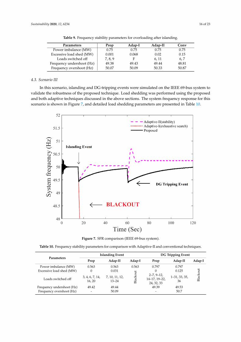
Sustainability 2020, 12, 6234 16 of 23
Table 9. Frequency stability parameters for overloading after islanding.
Parameters Prop Adap-I Adap-II ConvPower imbalance (MW) 0.75 0.75 0.75 0.75
Excessive load shed (MW) 0.001 0.068 0.02 0.15Loads switched off 7, 8, 9 F 6, 11 6, 7
Frequency undershoot (Hz) 49.38 49.43 49.44 48.81Frequency overshoot (Hz) 50.07 50.09 50.33 50.87
4.3. Scenario III
In this scenario, islanding and DG-tripping events were simulated on the IEEE 69-bus system tovalidate the robustness of the proposed technique. Load shedding was performed using the proposedand both adaptive techniques discussed in the above sections. The system frequency response for thisscenario is shown in Figure 7, and detailed load shedding parameters are presented in Table 10.Sustainability 2020, 12, x FOR PEER REVIEW 16 of 23
Sustainability 2020, 12, x; doi: FOR PEER REVIEW www.mdpi.com/journal/sustainability
Figure 7. SFR comparison (IEEE 69-bus system).
Table 10. Frequency stability parameters for comparison with Adaptive-II and conventional
techniques.
Parameters Islanding Event DG Tripping Event
Prop Adap-II Adap-I Prop Adap-II Adap-I
Power imbalance
(MW) 0.563 0.563 0.563 0.797 0.797
Black
ou
t
Excessive load shed
(MW) 0 0.031
Black
ou
t
0 0.125
Loads switched off 3, 4, 6, 7,
14, 16, 20
7,10,11,
12,13–24
2–7, 9–12, 14–
17, 19–22, 24,
32, 33
1–31, 33,
35, 36
Frequency
undershoot (Hz) 49.42 49.44 49.39 49.53
Frequency
overshoot (Hz) - 50.09 - 50.7
4.3.1. Islanding Event (69-Bus System)
The grid-coupling circuit breaker was disconnected at a simulation time of t = 15 s to create
intentional islanding for the IEEE 69-bus system. The total connected load in the system was 3.806
MW in this event, which was higher than the combined generation capacity of the DGs. Therefore,
the PICM estimated a power imbalance of 0.563 MW in the system, and the SICM calculated the
stability index of all load buses. Loads were arranged in ascending order according to stability index,
incorporating load priority. Critical loads were not shed in any case, hence the stability indices of
only non-critical and semi-critical loads are presented in Table 11.
Table 11. Stability indices for islanding and DG tripping (69-bus System).
Sr.
No
Islanding DG Tripping
Proposed Adaptive-II Proposed Adaptive-II
Figure 7. SFR comparison (IEEE 69-bus system).
Table 10. Frequency stability parameters for comparison with Adaptive-II and conventional techniques.
ParametersIslanding Event DG Tripping Event
Prop Adap-II Adap-I Prop Adap-II Adap-I
Power imbalance (MW) 0.563 0.563 0.563 0.797 0.797
Blac
koutExcessive load shed (MW) 0 0.031
Blac
kout 0 0.125
Loads switched off3, 4, 6, 7, 14,
16, 207, 10, 11, 12,
13–24
2–7, 9–12,14–17, 19–22,
24, 32, 33
1–31, 33, 35,36
Frequency undershoot (Hz) 49.42 49.44 49.39 49.53Frequency overshoot (Hz) - 50.09 - 50.7

Sustainability 2020, 12, 6234 17 of 23
4.3.1. Islanding Event (69-Bus System)
The grid-coupling circuit breaker was disconnected at a simulation time of t = 15 s to createintentional islanding for the IEEE 69-bus system. The total connected load in the system was 3.806 MWin this event, which was higher than the combined generation capacity of the DGs. Therefore, the PICMestimated a power imbalance of 0.563 MW in the system, and the SICM calculated the stability indexof all load buses. Loads were arranged in ascending order according to stability index, incorporatingload priority. Critical loads were not shed in any case, hence the stability indices of only non-criticaland semi-critical loads are presented in Table 11.
Table 11. Stability indices for islanding and DG tripping (69-bus System).
Sr.No
Islanding DG Tripping
Proposed Adaptive-II Proposed Adaptive-II
Rank Stability Rank Stability Rank Stability Rank Stability1 7 0.4995 7 0.4995 7 - 7 -2 23 0.5135 23 0.5135 14 - 10 -3 22 0.5179 22 0.5179 16 - 11 -4 21 0.5344 21 0.5344 4 - 12 -5 14 0.5399 14 0.5399 6 - 13 -6 16 0.5987 16 0.5987 20 - 14 -7 17 0.6075 17 0.6075 3 - 15 -8 18 0.6108 18 0.6108 11 0.2039 16 -9 11 0.6201 11 0.6201 23 0.2084 17 -
10 15 0.6276 15 0.6276 22 0.2089 18 -11 13 0.6440 13 0.6440 21 0.2171 19 -12 20 0.6483 20 0.6483 17 0.2233 20 -13 12 0.6638 12 0.6638 18 0.2255 21 -14 10 0.6731 10 0.6731 10 0.2298 22 -15 24 0.6896 24 0.6896 15 0.2321 23 -16 19 0.6896 19 0.6896 13 0.2332 24 -17 4 0.7071 4 0.7071 12 0.2357 4 0.234318 9 0.7128 9 0.7128 9 0.2403 9 0.251919 1 0.7290 1 0.7290 8 0.2449 8 0.25220 8 0.7310 8 0.7310 5 0.2562 5 0.258721 2 0.7348 2 0.7348 2 0.2762 6 0.267222 3 0.7538 3 0.7538 1 0.2813 2 0.276523 5 0.7704 5 0.7704 24 0.2836 3 0.276624 6 0.7848 6 0.7848 19 0.2836 1 0.283725 31 0.5748 31 0.5748 31 0.2283 31 0.237926 30 0.5806 30 0.5806 30 0.2306 30 0.240427 29 0.5974 29 0.5974 29 0.2389 29 0.24928 28 0.6144 28 0.6144 28 0.2469 28 0.257429 27 0.6254 27 0.6254 27 0.2522 27 0.262930 26 0.6399 26 0.6399 26 0.2591 36 0.267331 25 0.6746 25 0.6746 36 0.267 26 0.270232 36 0.7151 36 0.7151 35 0.276 35 0.276333 33 0.7303 33 0.7303 25 0.2767 25 0.288534 35 0.7344 35 0.7344 33 0.3233 33 0.33135 32 0.7825 32 0.7825 32 0.3559 32 0.364136 34 0.7989 34 0.7989 34 0.365 34 0.3733
Colored boxes show the load shed in the current event.
Sustainability 2020, 12, x FOR PEER REVIEW 12 of 23
Sustainability 2020, 12, x; doi: FOR PEER REVIEW www.mdpi.com/journal/sustainability
MW and excessive load shed amounts of 0.453 MW and 0.57 MW for the Adaptive-I, Adaptive-II,
and conventional techniques, respectively.
Table 5. Stability indices for the islanding event.
Sr. No Proposed Adaptive-I Adaptive-II Conventional
Rank Stability Rank Stability Rank Stability Rank Stability
1 7 0.0757 7 0.0757 7 0.0757 7 0.0757
2 6 0.1686 6 0.1686 6 0.1686 6 0.1686
3 11 0.236 11 0.236 11 0.236 11 0.236
4 9 0.313 9 0.313 9 0.313 9 0.313
5 10 0.3161 10 0.3161 10 0.3161 10 0.3161
6 2 0.3267 2 0.3267 2 0.3267 2 0.3267
7 1 0.3336 1 0.3336 1 0.3336 1 0.3336
8 4 0.3448 4 0.3448 4 0.3448 4 0.3448
9 8 0.3491 8 0.3491 8 0.3491 8 0.3491
10 5 0.3619 5 0.3619 5 0.3619 5 0.3619
11 3 0.4244 3 0.4244 3 0.4244 3 0.4244
12 14 0.1975 14 0.1975 14 0.1975 14 0.1975
13 15 0.2487 15 0.2487 15 0.2487 15 0.2487
14 16 0.2644 16 0.2644 16 0.2644 16 0.2644
15 13 0.2964 13 0.2964 13 0.2964 13 0.2964
16 12 0.4083 12 0.4083 12 0.4083 12 0.4083
17 18 0.0874 18 0.0874 18 0.0874 18 0.0874
18 17 0.2291 17 0.2291 17 0.2291 17 0.2291
19 20 0.2318 20 0.2318 20 0.2318 20 0.2318
20 19 0.2842 19 0.2842 19 0.2842 19 0.2842
Colored boxes show the load shed in the current event. proposed scheme, adaptive-I
scheme, adaptive-II scheme and conventional scheme
Table 6. Frequency stability parameters for comparison (Scenario I).
Parameters Islanding Event DG-Tripping Event
Prop Adap-I Adap-II Conv Prop Adap-I Adap-II Conv
Power imbalance (MW) 0.39 0.39 0.39 0.39 1.891 1.891 1.891 1.89
Load shed amount (MW) 0.38 0.32 0.453 0.57 1.890 2.071 2.304 2.127
Excessive load shed (MW) −0.001 −0.007 0.063 0.18 −0.001 0.18 0.414 0.237
Loads switched off 2, 11 b, d 7 1–5 1, 4, 5, 6, 7, 10, 15 a–g 1–11,14 1–13
Frequency undershoot (Hz) 49.453 49.452 49.48 49.1 48.8 49 48.86 48.54
Frequency overshoot (Hz) - - 50.28 50.5 - 50.28 53.6 51.7
4.1.2. DG Tripping in an Islanded System
For validation of the proposed method, one of the DGs was disconnected from the system during
the islanded mode. The bio-mass DG was disconnected at time t = 60 s when the system was operating
in islanded mode. Figure 5 shows the frequency response of the system, and frequency stability
parameters are compared in Table 6. The conventional technique shed loads ranked 6–13 in addition
to loads shed in Scenario 1, resulting in a frequency overshoot of 51.7 Hz. Loads ranked ‘a’ to ‘g’ in
Table 4 were shed for the Adaptive-I technique. It is visible from Figure 5 that frequency was stabled
for the proposed technique without any overshoot, as compared to an overshoot of 50.28 Hz, 53.6
HZ, and 51.7 Hz for the Adaptive-I, Adaptive-II, and conventional techniques, respectively.
The overshoot in the SFR for the Adaptive-I technique was due to the fact that the power
imbalance was higher than the total random priority loads, and a fixed priority load was
disconnected in addition to all random priority loads. Therefore, an additional 0.18 MW load was
shed for the Adaptive-I technique, as can be seen in Table 6. However, the Adaptive-II technique
proposed scheme,
Sustainability 2020, 12, x FOR PEER REVIEW 12 of 23
Sustainability 2020, 12, x; doi: FOR PEER REVIEW www.mdpi.com/journal/sustainability
MW and excessive load shed amounts of 0.453 MW and 0.57 MW for the Adaptive-I, Adaptive-II,
and conventional techniques, respectively.
Table 5. Stability indices for the islanding event.
Sr. No Proposed Adaptive-I Adaptive-II Conventional
Rank Stability Rank Stability Rank Stability Rank Stability
1 7 0.0757 7 0.0757 7 0.0757 7 0.0757
2 6 0.1686 6 0.1686 6 0.1686 6 0.1686
3 11 0.236 11 0.236 11 0.236 11 0.236
4 9 0.313 9 0.313 9 0.313 9 0.313
5 10 0.3161 10 0.3161 10 0.3161 10 0.3161
6 2 0.3267 2 0.3267 2 0.3267 2 0.3267
7 1 0.3336 1 0.3336 1 0.3336 1 0.3336
8 4 0.3448 4 0.3448 4 0.3448 4 0.3448
9 8 0.3491 8 0.3491 8 0.3491 8 0.3491
10 5 0.3619 5 0.3619 5 0.3619 5 0.3619
11 3 0.4244 3 0.4244 3 0.4244 3 0.4244
12 14 0.1975 14 0.1975 14 0.1975 14 0.1975
13 15 0.2487 15 0.2487 15 0.2487 15 0.2487
14 16 0.2644 16 0.2644 16 0.2644 16 0.2644
15 13 0.2964 13 0.2964 13 0.2964 13 0.2964
16 12 0.4083 12 0.4083 12 0.4083 12 0.4083
17 18 0.0874 18 0.0874 18 0.0874 18 0.0874
18 17 0.2291 17 0.2291 17 0.2291 17 0.2291
19 20 0.2318 20 0.2318 20 0.2318 20 0.2318
20 19 0.2842 19 0.2842 19 0.2842 19 0.2842
Colored boxes show the load shed in the current event. proposed scheme, adaptive-I
scheme, adaptive-II scheme and conventional scheme
Table 6. Frequency stability parameters for comparison (Scenario I).
Parameters Islanding Event DG-Tripping Event
Prop Adap-I Adap-II Conv Prop Adap-I Adap-II Conv
Power imbalance (MW) 0.39 0.39 0.39 0.39 1.891 1.891 1.891 1.89
Load shed amount (MW) 0.38 0.32 0.453 0.57 1.890 2.071 2.304 2.127
Excessive load shed (MW) −0.001 −0.007 0.063 0.18 −0.001 0.18 0.414 0.237
Loads switched off 2, 11 b, d 7 1–5 1, 4, 5, 6, 7, 10, 15 a–g 1–11,14 1–13
Frequency undershoot (Hz) 49.453 49.452 49.48 49.1 48.8 49 48.86 48.54
Frequency overshoot (Hz) - - 50.28 50.5 - 50.28 53.6 51.7
4.1.2. DG Tripping in an Islanded System
For validation of the proposed method, one of the DGs was disconnected from the system during
the islanded mode. The bio-mass DG was disconnected at time t = 60 s when the system was operating
in islanded mode. Figure 5 shows the frequency response of the system, and frequency stability
parameters are compared in Table 6. The conventional technique shed loads ranked 6–13 in addition
to loads shed in Scenario 1, resulting in a frequency overshoot of 51.7 Hz. Loads ranked ‘a’ to ‘g’ in
Table 4 were shed for the Adaptive-I technique. It is visible from Figure 5 that frequency was stabled
for the proposed technique without any overshoot, as compared to an overshoot of 50.28 Hz, 53.6
HZ, and 51.7 Hz for the Adaptive-I, Adaptive-II, and conventional techniques, respectively.
The overshoot in the SFR for the Adaptive-I technique was due to the fact that the power
imbalance was higher than the total random priority loads, and a fixed priority load was
disconnected in addition to all random priority loads. Therefore, an additional 0.18 MW load was
shed for the Adaptive-I technique, as can be seen in Table 6. However, the Adaptive-II technique
adaptive-II scheme.
The SFR in Figure 7 depicts that the adaptive technique based on an exhaustive search couldnot perform load shedding in time and resulted in a blackout. Possible combinations for 48 loadsof the IEEE 69-bus system reached beyond 281 billion. Therefore, it was infeasible for a practicalcomputer system to store and evaluate all combinations, whereas the adaptive technique based on the

Sustainability 2020, 12, 6234 18 of 23
stability index shed the unstable loads from Table 11 sequentially and resulted in an overshoot of 50.09(Figure 7). This overshoot in the SFR suggested that an additional load of 0.031 MW had been shed.On the other hand, the SFR for the proposed technique in Figure 7 indicates indicated that an accurateamount of load was shed to avoid any overshoot. The stability index table and detailed load sheddingparameters in Table 10 indicate that minimum and comparatively unstable non-critical loads wereselected for shedding to ensure stable islanding operation of the distribution system.
4.3.2. DG-Tripping Event (69-Bus System)
A DG was intentionally desynchronized from the islanded system to validate the performance ofthe proposed technique in case of a suspected cascaded blackout. One of the DGs in the system wasdisconnected at a simulation time of t = 60 s when the system was operating in stable islanding condition.The PICM estimated a power imbalance of 0.797 MW in the system for this event. Stability indices ofconnected loads for this event are arranged in ascending order and shown in Table 11. Stability indices ofalready disconnected loads in the islanding event are replaced by dashes in the table. Table 10 indicatesthat all the non-critical and semi-critical loads except loads ranked 32 and 34 were disconnected for theadaptive technique based on the stability index, shedding an additional 0.125 MW load. The excessiveload shedding caused a high overshoot of 50.7 in the SFR for the Adaptive-II technique. The SFR inFigure 7 and load shedding parameters in Table 10 show that proposed techniques performed a betterload shedding without any overshoot in the SFR by disconnecting a combination of two semi-criticaland 19 non-critical loads in this event.
It is obvious to conclude from the simulation results in this scenario that the performance of theproposed technique was not affected by increasing the number of loads. However, the Adaptive-Itechnique based on an exhaustive search failed to find the best combination of loads to be shed atan appropriate time, when all the loads in the system were used for load shedding, and this led thesystem frequency to drop in no time, which resulted in a cascaded blackout. This problem occurredbecause there are 281 trillion possible combinations for 48 loads. The search space required to evaluatethese combinations became huge and practically infeasible, which increased the computational time.Hence the system collapsed before the load shedding took place, which can be noticed from Figure 7.Furthermore, the connected load after the islanding and DG-tripping events was maximum for theproposed technique.
5. Discussions
The main objective of all the load shedding techniques was to maximize load connection in thesystem with a stable frequency. It is visible from the comparison of results that a maximum load wasconnected in the system for the proposed technique. Moreover, the proposed load shedding schemeselected an optimal combination of loads for any contingency, incorporating load priority and thestability index to produce an SFR without any significant overshoot. The advantage of incorporatingload priority and the stability index simultaneously for a load shedding technique is apparent fromthe SFR in Figure 8. The proposed technique was simulated with three different objective functions,as shown in Equations (11) to (13), for load shedding. The basic objective function for the proposedmathematical model found an optimal combination of loads that exactly matched an estimated powerimbalance, shown in Equation (11).
OF1 = min
N∑i=1
Ai.xi + δ.w
(11)
OF2 = min
N∑i=1
SIi.xi + δ.w
(12)
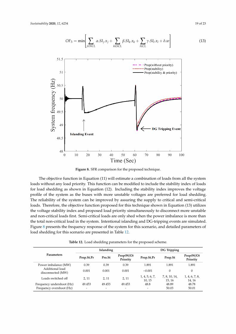
Sustainability 2020, 12, 6234 19 of 23
OF3 = min
∑j∈NCL
α.SI j.x j +∑
k∈SCL
β.SIk.xk +∑l∈CL
γ.SIl.xl + δ.w
(13)
Sustainability 2020, 12, x FOR PEER REVIEW 19 of 23
Sustainability 2020, 12, x; doi: FOR PEER REVIEW www.mdpi.com/journal/sustainability
Figure 8. SFR comparison for the proposed technique.
The objective function in Equation (11) will estimate a combination of loads from all the system
loads without any load priority. This function can be modified to include the stability index of loads
for load shedding as shown in Equation (12). Including the stability index improves the voltage
profile of the system as the buses with more unstable voltages are preferred for load shedding. The
reliability of the system can be improved by assuring the supply to critical and semi-critical loads.
Therefore, the objective function proposed for this technique shown in Equation (13) utilizes the
voltage stability index and proposed load priority simultaneously to disconnect more unstable and
non-critical loads first. Semi-critical loads are only shed when the power imbalance is more than the
total non-critical load in the system. Intentional islanding and DG-tripping events are simulated.
Figure 8 presents the frequency response of the system for this scenario, and detailed parameters of
load shedding for this scenario are presented in Table 12.
Table 12. Load shedding parameters for the proposed scheme.
Parameters
Islanding DG Tripping
Prop.St.Pr Pro.St Prop(W/O)
Priority Prop.St.Pr Prop.St
Prop(W/O)
Priority
Power imbalance (MW) 0.39 0.39 0.39 1.891 1.891 1.891
Additional load
disconnected (MW) 0.001 0.001 0.001 −0.001 0 0
Loads switched off 2, 11 2, 11 2, 11 1, 4, 5, 6, 7,
10, 15
7, 8, 10,
14, 15, 16
1, 4, 6, 7, 8,
14, 16
Frequency undershoot
(Hz) 49.453 49.453 49.453 48.8 48.89 48.78
Frequency overshoot
(Hz) - - - - 50.03 50.01
5.1. Islanding Event
The grid-coupling circuit breaker was operated at a simulation time of t = 15 s to implement
intentional islanding. The generation capacity of all DGs in the system was less than the total load
demand, and frequency started decreasing. The proposed PIFM estimated a power imbalance of 0.39
Figure 8. SFR comparison for the proposed technique.
The objective function in Equation (11) will estimate a combination of loads from all the systemloads without any load priority. This function can be modified to include the stability index of loadsfor load shedding as shown in Equation (12). Including the stability index improves the voltageprofile of the system as the buses with more unstable voltages are preferred for load shedding.The reliability of the system can be improved by assuring the supply to critical and semi-criticalloads. Therefore, the objective function proposed for this technique shown in Equation (13) utilizesthe voltage stability index and proposed load priority simultaneously to disconnect more unstableand non-critical loads first. Semi-critical loads are only shed when the power imbalance is more thanthe total non-critical load in the system. Intentional islanding and DG-tripping events are simulated.Figure 8 presents the frequency response of the system for this scenario, and detailed parameters ofload shedding for this scenario are presented in Table 12.
Table 12. Load shedding parameters for the proposed scheme.
ParametersIslanding DG Tripping
Prop.St.Pr Pro.St Prop(W/O)Priority Prop.St.Pr Prop.St Prop(W/O)
Priority
Power imbalance (MW) 0.39 0.39 0.39 1.891 1.891 1.891Additional load
disconnected (MW) 0.001 0.001 0.001 −0.001 0 0
Loads switched off 2, 11 2, 11 2, 11 1, 4, 5, 6, 7,10, 15
7, 8, 10, 14,15, 16
1, 4, 6, 7, 8,14, 16
Frequency undershoot (Hz) 49.453 49.453 49.453 48.8 48.89 48.78Frequency overshoot (Hz) - - - - 50.03 50.01

Sustainability 2020, 12, 6234 20 of 23
5.1. Islanding Event
The grid-coupling circuit breaker was operated at a simulation time of t = 15 s to implementintentional islanding. The generation capacity of all DGs in the system was less than the total loaddemand, and frequency started decreasing. The proposed PIFM estimated a power imbalance of0.39 MW in this case and activated the SICM and ILSM. The SICM then processed the system data tocalculate the stability indices of all load buses and transmitted them to the ILSM. The load sheddingmodule found the optimal combination of loads to be shed as directed by the objective functions.Stability indices of all loads are summarized in Table 7. It is evident from Figure 8 that the systemfrequency response (SFR) was similar in the islanding event for all three proposed objective functions.This was due to the fact that the power imbalance was smaller and the mathematical model founda unique solution which fulfilled constraints for all three objective functions. Hence optimal loadshedding was performed. Table 12 also shows that loads ranked 2 and 11 were selected for sheddingwith minimum error and no overshoot.
5.2. DG Tripping in Islanded System
A distribution system operating in islanding is vulnerable to instability due to unplanned disconnectionof a DG, which may yield a cascaded blackout. Hence a load shedding scheme should be able to compensatethis scenario to prevent the system from blackout. To validate the proposed technique, the biggest DG inthe system was disconnected at a simulation time of t = 60 s. The system frequency declined rapidly andthe PICM actuated load shedding and it forecasted a power imbalance of 1.891 MW.
The SFR in Figure 8 for the DG-tripping event reveals that accurate load shedding was performedfor the proposed technique with all three objective functions. An almost similar amount of load wasshed with the three different solutions for all discussed objective functions. The stability index of allloads for this contingency is shown in Table 7. It can be observed from Tables 7 and 12 that semi-criticalloads 14, 15, and 16 were switched off when the proposed technique was tested with the load prioritybased on the stability index only. On the other hand, comparatively stable and semi-critical loads14 and 16 were shed when the proposed technique was tested without any load priority. Therefore, it isconclusive that the proposed technique performed better and disconnected more unstable and non-criticalloads when loads were prioritized based on both their type and stability index. Semi-critical and stableloads were disconnected from the system when it was simulated without any load priority and stability.Furthermore, it can be observed from Figure 8 and Table 7 that a load shedding solution that incorporatedthe stability index and load priority simultaneously increased the reliability of the power supply for criticalloads and improved the stability of load buses. Hence, the proposed load shedding scheme based on MILPoptimization, stability index, and load priority solved the load shedding problem much more efficientlyand its performance was not affected, regardless of the number of loads.
6. Conclusions
A high number of DGs based on renewable sources in the distribution system increases therisk of blackouts when the system is disconnected from the grid. Blackouts can be avoided byperforming load shedding to mitigate the unbalanced supply and load demand. Excessive, sequential,and random load shedding results in frequency response overshoot. The absence of load priorityendangers the functionality of vital loads. This paper presents a robust load shedding scheme for thesuccessful islanding operation of the distribution system. The frequency rate of change is used toestimate power imbalance, and MILP optimization finds the optimal combination from the prioritizedloads. The proposed scheme was validated for different events such as islanding, generator tripping,and overloading on a Malaysian distribution network and an IEEE 69-bus system. Simulation resultsshowed that the proposed technique produces better results and smoother frequency response ascompared to adaptive techniques. The adaptive technique based on an exhaustive search is applicableto only a limited number of loads. Increasing the number of loads yields a huge number of possible

Sustainability 2020, 12, 6234 21 of 23
combinations and thus requires a large memory size to store these combinations (281 trillion for69-bus system loads). Moreover, it is infeasible to evaluate all the possible combinations that willrequire high computational time. Therefore, a blackout will occur for the IEEE 69-bus system dueto the delayed response and infeasible computation memory requirement for an exhaustive search.The adaptive technique, based on a stability index of loads, increases the system voltage stabilityby disconnecting more unstable loads on priority to avoid unnecessary operation of under-voltageprotection; however, sequential shedding of unstable loads yields excessive load shedding, resulting inovershoot, and endangers the stability of system frequency. On the other hand, prioritized shedding ofcomparatively more unstable non-critical loads in the proposed technique produces a smooth recoveryof frequency response without any overshoot. This proves that the proposed technique is an optimalsolution to the load shedding problem for any distribution network.
7. Future Works
The high share of non-synchronous generation sources in future power systems presents low orno inertia. As a result, power imbalance estimation for load shedding based on the rate of change offrequency and inertia of the system may not be reliable and efficient in practice. Moreover, AC/DCmicrogrids are gaining traction in modern power systems. Therefore, future work on this techniquewill be to propose a new load shedding scheme to mitigate the effect of low inertia of the system.Furthermore, the bidirectional power share in modern AC/DC microgrids will be investigated to avoidload shedding and maximize the power supply in the system.
Author Contributions: Conceptualization, S.S. and M.A.M.; methodology, S.S.; software, H.M. (HasmainiMohamed); validation, H.M. (Hazlie Mokhils) and M.A.M.; formal analysis, N.N.M.; investigation, M.O. andJ.A.L.; resources, S.S., H.M. (Hazlie Mokhils) and A.P.; data curation, S.S.; writing—original draft preparation, S.S.;writing—review and editing, H.M. (Hazlie Mokhils), N.N.M. and J.A.L.; supervision, H.M. (Hazlie Mokhils) andM.O.; project administration, H.M. (Hazlie Mokhils); funding acquisition, H.M. (Hasmaini Mohamed) and A.P.All authors have read and agreed to the published version of the manuscript.
Funding: This research received no external funding.
Acknowledgments: The authors thank the University of Malaya for supporting this research under RU GrantFaculty Program (Grant code: GPF055A-2018).
Conflicts of Interest: The authors declare no conflict of interest.
Nomenclature
Hi Inertia constant of the ith generatorM Number of DGs connected in the systemN Total number of loads in the systemPDGi Total dispatched power of DGiMaxDGi Maximum generation capacity of DGid(fsys)/dt Rate of change of the system frequencyPi, Qi, Ri, and Xi, Active power, reactive power, resistance, and reactance, respectivelyNCL, SCL, and CL Non-critical, semi-critical, and critical load sets, respectivelyw Dummy variable for MILP problemα, β, and γ Coefficients of the linear problem for load priority and optimizationfn Nominal frequencySIi Stability index of ith loadPSR Total spinning reservesxi Load’s circuit breaker status∆P Power imbalancePLi Real-time load value at bus ifi Frequency of ith generatorVsi Sending end voltage for the ith busδ Coefficient of dummy variable
Sustainability 2020, 12, 6234 22 of 23
References
1. Xu, T.P.D.; Li, Z.; Shieh, S.S.; Jang, S.S. Efficiency improvement of cogeneration system using statistical model.Energy Convers. Manag. 2013, 68, 169–176.
2. Williams, J.H.; DeBenedictis, A.; Ghanadan, R.; Mahone, A.; Moore, J.; Morrow, W.R., III; Price, S.; Torn, M.S.The Technology Path to Deep Greenhouse Gas Emissions Cuts by 2050: The Pivotal Role of Electricity. Science2012, 335, 53–59. [CrossRef] [PubMed]
3. Santamouris, M.; Cartalis, C.; Synnefa, A.; Kolokotsa, D. On the impact of urban heat island and globalwarming on the power demand and electricity consumption of buildings—A review. Energy Build. 2015, 98,119–124. [CrossRef]
4. Narula, K.; Nagai, Y.; Pachauri, S. The role of Decentralized Distributed Generation in achieving universalrural electrification in South Asia by 2030. Energy Policy 2012, 47, 345–357. [CrossRef]
5. Silva, M.; Morais, H.; Vale, Z. An integrated approach for distributed energy resource short-term schedulingin smart grids considering realistic power system simulation. Energy Convers. Manag. 2012, 64, 273–288.[CrossRef]
6. Barker, P.P.; Mello, R.W.D. Determining the impact of distributed generation on power systems. I.Radial distribution systems. In Proceedings of the 2000 Power Engineering Society Summer Meeting(Cat. No.00CH37134), Seattle, WA, USA, 16–20 July 2000; pp. 1645–1656.
7. Azmy, A.M.; Erlich, I. Impact of distributed generation on the stability of electrical power system.In Proceedings of the IEEE Power Engineering Society General Meeting, San Francisco, CA, USA, 16 June2005; pp. 1056–1063.
8. Xypolytou, E.; Gawlik, W.; Zseby, T.; Fabini, J. Impact of Asynchronous Renewable Generation Infeed onGrid Frequency: Analysis Based on Synchrophasor Measurements. Sustainability 2018, 10, 1605. [CrossRef]
9. Lopes, J.A.P.; Moreira, C.L.; Madureira, A.G. Defining control strategies for MicroGrids islanded operation.IEEE Trans. Power Syst. 2006, 21, 916–924. [CrossRef]
10. Girgis, A.A.; Ham, F.M. A New FFT-Based Digital Frequency Relay for Load Shedding. IEEE Trans. Power Syst.1982, 2, 433–439. [CrossRef]
11. Anderson, P.M.; Mirheydar, M. An adaptive method for setting underfrequency load shedding relays.IEEE Trans. Power Syst. 1992, 7, 647–655. [CrossRef]
12. Jiang, H.; Yan, G.; Ji, H.; Liu, L.; Shan, D. An improved under frequency load shedding scheme basedon rate of change of frequency. In Proceedings of the International Conference on Electrical and Control.Engineering (ICECE), Wuhan, China, 25–27 June 2010; pp. 292–3295.
13. Rafinia, A.; Moshtagh, J.; Rezaei, N. Stochastic optimal robust design of a new multi-stage under-frequencyload shedding system considering renewable energy sources. Int. J. Electr. Power Energy Syst. 2020, 118,105735. [CrossRef]
14. Chuvychin, V.N.; Gurov, N.S.; Venkata, S.S.; Brown, R.E. An adaptive approach to load shedding andspinning reserve control during underfrequency conditions. IEEE Trans. Power Syst. 1996, 11, 1805–1810.[CrossRef]
15. Ford, J.J.; Bevrani, H.; Ledwich, G. Adaptive load shedding and regional protection. Int. J. Electr.Power Energy Syst. 2009, 31, 611–618. [CrossRef]
16. Wang, Z.; Guo, L.; Wu, K.; Liu, W.; Zhou, J. Minimum load-shedding calculation approach considering loadsdifference. In Proceedings of the IEEE Innovative Smart Grid Technologies-Asia (ISGT Asia), Kuala Lampur,Malaysia, 20–23 May 2014; pp. 344–348.
17. Nourollah, S.; Aminifar, F.; Gharehpetian, G.B. A Hierarchical Regionalization-Based Load Shedding Plan toRecover Frequency and Voltage in Microgrid. IEEE Trans. Smart Grid. 2019, 10, 3818–3827. [CrossRef]
18. Hooshmand, R.; Moazzam, M.I. Optimal design of adaptive under frequency load shedding using artificialneural networks in isolated power system. Int. J. Electr. Power Energy Syst. 2012, 42, 220–228. [CrossRef]
19. Santos, A.Q.; Monaro, R.; Coury, D.; Oleskovicz, M. Real-time closed loop system controlled by an ArtificialNeural Network for estimation of the optimal load shedding. In Proceedings of the 12th IET InternationalConference on Developments in Power System Protection, Copenhagen, Denmark, 31 March–3 April 2014.
20. Moazzami, M.; Khodabakhshian, A.; Hooshmand, R.-A. A New Optimal Under-frequency Load-sheddingMethod Using Hybrid Culture–Particle Swarm Optimization–Co-evolutionary Algorithm and ArtificialNeural Networks. Electr. Power Compon. Syst. 2015, 43, 69–82. [CrossRef]
Sustainability 2020, 12, 6234 23 of 23
21. Amraee, T.; Darebaghi, M.G.; Soroudi, A.; Keane, A. Probabilistic under frequency load shedding consideringrocof relays of distributed generators. IEEE Trans. Power Syst. 2018, 33, 3587–3598. [CrossRef]
22. Çimen, H.; Aydın, M. Optimal Load Shedding Strategy for Selçuk University Power System with DistributedGeneration. Procedia-Soc. Behav. Sci. 2015, 195, 2376–2381. [CrossRef]
23. Khezri, R.; Golshannavaz, S.; Vakili, R.; Memar-Esfahani, B. Multi-layer fuzzy-based under-frequency loadshedding in back-pressure smart industrial microgrids. Energy 2017, 132, 96–105. [CrossRef]
24. Alhelou, H.H.; Hamedani-Golshan, M.E.; Njenda, T.C.; Siano, P. Wide-area measurement system-basedoptimal multi-stage under-frequency load-shedding in interconnected smart power systems usingevolutionary computing techniques. Appl. Sci. 2019, 9, 508. [CrossRef]
25. Santos, A.Q.; Shaker, H.R.; Jørgensen, B.N. A Holistic Fuzzy Measure for Load Priority in Under FrequencyLoad Shedding Schemes. In Proceedings of the International Symposium on Advanced Electrical andCommunication Technologies (ISAECT), Rabat-Kenitra, Morocco, 21–23 November 2018; pp. 1–6.
26. López, K.; Pérez, S.; Rodríguez, L. Optimal under voltage load shedding based on voltage stability index.Ing. Investig. 2016, 36, 43–50.
27. Yusof, N.A.; Rosli, H.M.; Mokhlis, H.; Karimi, M.; Selvaraj, J.; Sapari, N.M. A new under-voltage loadshedding scheme for islanded distribution system based on voltage stability indices. IEEE Trans. Power Syst.2017, 12, 665–675. [CrossRef]
28. Laghari, J.A.; Mokhlis, H.; Karimi, M.; Bakar, A.H.A.; Mohamad, H. A New Under-Frequency Load SheddingTechnique Based on Combination of Fixed and Random Priority of Loads for Smart Grid Applications.IEEE Trans. Power Syst. 2015, 30, 2507–2515. [CrossRef]
29. Dreidy, M.; Mokhlis, H.; Mekhilef, S.J.E. Application of meta-heuristic techniques for optimal load sheddingin islanded distribution network with high penetration of solar PV generation. Energies 2017, 10, 150.[CrossRef]
30. Laghari, J.A.; Mokhlis, H.; Bakar, A.H.A.; Mohamad, H. Application of computational intelligence techniquesfor load shedding in power systems: A review. Energy Convers. Manag. 2013, 75, 130–140. [CrossRef]
31. Chakravorty, M.; Das, D. Voltage stability analysis of radial distribution networks. Int. J Electr. PowerEnergy Syst. 2001, 23, 129–135. [CrossRef]
32. Muhammad, M.A.; Mokhlis, H.; Naidu, K.; Amin, A.; Franco, J.F.; Othman, M. Distribution NetworkPlanning Enhancement via Network Reconfiguration and DG Integration using Dataset Approach and WaterCycle Algorithm. J. Mod. Power Syst. Clean Energy 2020, 8, 86–93. [CrossRef]
© 2020 by the authors. Licensee MDPI, Basel, Switzerland. This article is an open accessarticle distributed under the terms and conditions of the Creative Commons Attribution(CC BY) license (http://creativecommons.org/licenses/by/4.0/).