A modal-spectral model for flanking transmissions

J. Poblet-Puig∗1

1Laboratori de Calcul Numeric, E.T.S. d’Enginyers de Camins, Canals

i Ports de Barcelona, Universitat Politecnica de Catalunya

August 7, 2016

Abstract

A model for the prediction of direct and indirect (flanking) sound transmis-sions is presented. It can be applied to geometries with extrusion symmetry.The structures are modelled with spectral finite elements. The acoustic do-mains are described by means of a modal expansion of the pressure field andmust be cuboid-shaped. These reasonable simplifications in the geometry al-low the use of more efficient numerical methods. Consequently the coupledvibroacoustic problem in structures such as junctions is efficiently solved. Thevibration reduction index of T-junctions with acoustic excitation and with pointforce excitation is compared. The differences due to the excitation type obeyquite general trends that could be taken into account by prediction formulas.However, they are smaller than other uncertainties not considered in practice.The model is also used to check if the sound transmissions of a fully vibroacous-tic problem involving several flanking paths can be reproduced by superpositionof independent paths. There exist some differences caused by the interactionbetween paths, which are more important at low frequencies.

1 Introduction

Predictions of the direct and indirect (flanking) sound transmission are importantin order to make proper acoustic designs of buildings, ships or train wagons. Butthe simulations done by means of the finite element method (FEM), the boundaryelement method (BEM) or other deterministic techniques based on space discretisationare often time consuming and computationally expensive due to several reasons: theneed to cover a wide frequency range of audible noise, the mandatory use of smallerelements when frequency increases, the large dimensions of the physical domains tobe considered or the big number of situations to be analysed in order to understandthe problem and provide practical design rules.

∗correspondence: UPC, Campus Nord B1, Jordi Girona 1, E-08034 Barcelona, Spain, e-mail:jordi.poblet@upc.edu

1

This is especially critical in the field of building acoustics where numerical simula-tions are often restricted to the low-frequency range and/or two-dimensional problems.Very often the interest is focused to describe the behaviour of a single component (i.e.sound transmission through a single wall, vibration response of a junction). However,the problem of flanking transmission is global in the sense that it affects several acous-tic domains and more or less complex and big structures. It causes computationalrequirements to be larger and quite often unaffordable.

The use of semi-analytical models or statistical techniques such as Statistical En-ergy Analysis (SEA) [1] which hypotheses are valid only at high frequencies is verycommon in order to complement and cover the whole frequency range of interest. Animportant example is the global model proposed in the EN-12354 [2]. It accountsfor all transmission types (direct and flanking) and it is based on a first order SEAformulation [3, 4]. The main input required by the model in order to deal with flank-ing transmissions is the vibration reduction index. Recent researches try to providepractical design data by studying the structural junctions in the laboratory [5, 6], bymeans of finite element models [7], using wave approach [8], or wave-based or spectralfinite elements (SFEM) [9, 10, 11]. All of them are restricted to the study of vibrationtransmissions through the junction.

In the present work, a model is formulated and implemented in a computer softwarein order to complement these simulations but including now the acoustic part of theproblem (i.e. rooms that are separated by the junction). The starting point is themodel developed in [9]. The vibroacoustic problem to be analysed is restricted togeometries with extrusion symmetry where the acoustic domains are cuboid-shaped.This allows the attainment of a computationally efficient formulation. It uses spectralfinite elements [12, 13, 14] for the structure part and expand the pressure field in theacoustic domains in terms of the analytical expression of the eigenfunctions. All thesekeep the model general enough to deal with a great variety of junctions and structures.The results obtained are fully equivalent to a FEM simulation. So, they are valid forall frequencies and are not subjected to hypotheses of physical nature such as the onesrequired by SEA (they are only satisfied when the frequency is high enough in orderto guarantee large modal density of each subsystem among other aspects). Since themodel is oriented to reduce the computational costs of FEM or BEM for problemssatisfying the restrictions mentioned above, a larger frequency range can be simulated.Moreover, an ensemble of situations can be considered as an attempt to reproducethe uncertainty and statistical nature of the physical phenomenon at mid frequencieswhere the modal overlap starts to be important.

The contributions of the research are:

• Formulation, implementation and testing of a deterministic model accountingfor extrusion symmetry vibroacoustic problems in a wide frequency range withsmaller computation costs than other element-based methods

• Coupling of the SFEM for shells with the modal expansion of cuboid acousticdomains.

• Computation of the vibration reduction indices for heavy junctions with acousticexcitation (instead of mechanical or point forces)

2

Both components of the model presented here: the use of modal analysis to de-scribe the pressure field in acoustic cavities or rooms and the derivation of spectralor wave-based elements are not new. However, to the best of the author knowledgea model combining these techniques and its application to the problem of flankingtransmissions has not been presented before.

Analytical modal expansion of the pressure field in cavities is a good option when:i)the shape of the domains to be studied is simple but the dimensions large; ii)thecomputational costs must be optimised at maximum; iii)it is important to cover awide frequency range to gain knowledge on the physics of the problem and iv)thecoupling is weak enough in order to consider the in vacuo modes of each sub-domainof the problem. This technique, recently reviewed in [15], has been considered inthe study of a cuboid-shaped cavity coupled with a rectangular plate [16, 17, 18],the sound transmission between cuboid-shaped rooms separated by: a single wall[19, 20, 21, 22, 23, 24, 25, 26, 27], a double wall [28, 29], cavities of double walls [30],slits and holes [31] or the transmissions between continuous plates coupled to rooms[32]. Other models combine a modal description in one plane with a description infunction of plane waves propagating in positive and negative direction normal to themodal plane which helps in order to impose the continuity of normal velocity. Seefor example [33] with an application to the sound transmission through cross sectionsthat can be composed of an aperture and flexible structures, [23, 34, 35] for soundtransmission problems, or [36] where in a problem of the sound transmission througha single wall, the direction orthogonal to the wall is infinite.

The most common option is to consider normal modes (case of rigid walls or nullnormal velocity in all the boundaries), see the general theory in [37]. Their analyticalexpression is simple, they have interesting orthogonality properties and provide goodapproximation when the absorption or damping is not very high. This is the optionchosen here. However, other options better adapted to satisfy the absorbing (Robin)boundary conditions [38] or the pressure field around a point source [39] exist.

The dynamic stiffness methods and the SFEM are also a good option to deal withthe study of structural vibration in a wide frequency range. They have been used,among others, to predict the vibration behaviour of structures composed of panels[40]. Most of these methods require the assumption of some geometry simplification.But recent formulations try to extend their use to more general structures, for examplecomposed of rectangular plates [41, 42, 43].

The manuscript is organised as follows. The model is presented in Section 2. Theinterest is focused on the way how the SFEM and the modal expansion of the acousticdomains are coupled. The numerical examples are shown in Section 3, including acomparison with the finite strip method (FSM) and the parametric analysis of theT-shaped junction. The discussion of the results and possible future improvements isdone in Section 4 and the paper is finished with the conclusions of Section 5.

3

2 Method and theory

2.1 Model overview

The goal is to formulate a deterministic model that could deal with vibroacousticproblems of quite large dimensions (which is often the situation in building acous-tics), in a wide frequency range, with reduced computational costs and consideringstructures a bit more complex than a single or double wall. The price to satisfy thisrequirements is to assume some simplifications in geometry and boundary conditionsin order to use numerical techniques less generic but more efficient than FEM orBEM. SFEM allows the description of the structure with few nodes and elements.The modal expansion of the acoustic domains provides a quite accurate estimationof the pressure field with few modes (much less than nodes in the equivalent FEMdiscretisation).

Ly

X, U

Y, VZ, W

Zone 1xl

x, u

z, w

y, vZone 3

Zone 2

Receiving Room

Sending Room

x

y

z

(a)

L0

xl

1,jk

2,rk

z

x

z

x

1

2

(b)

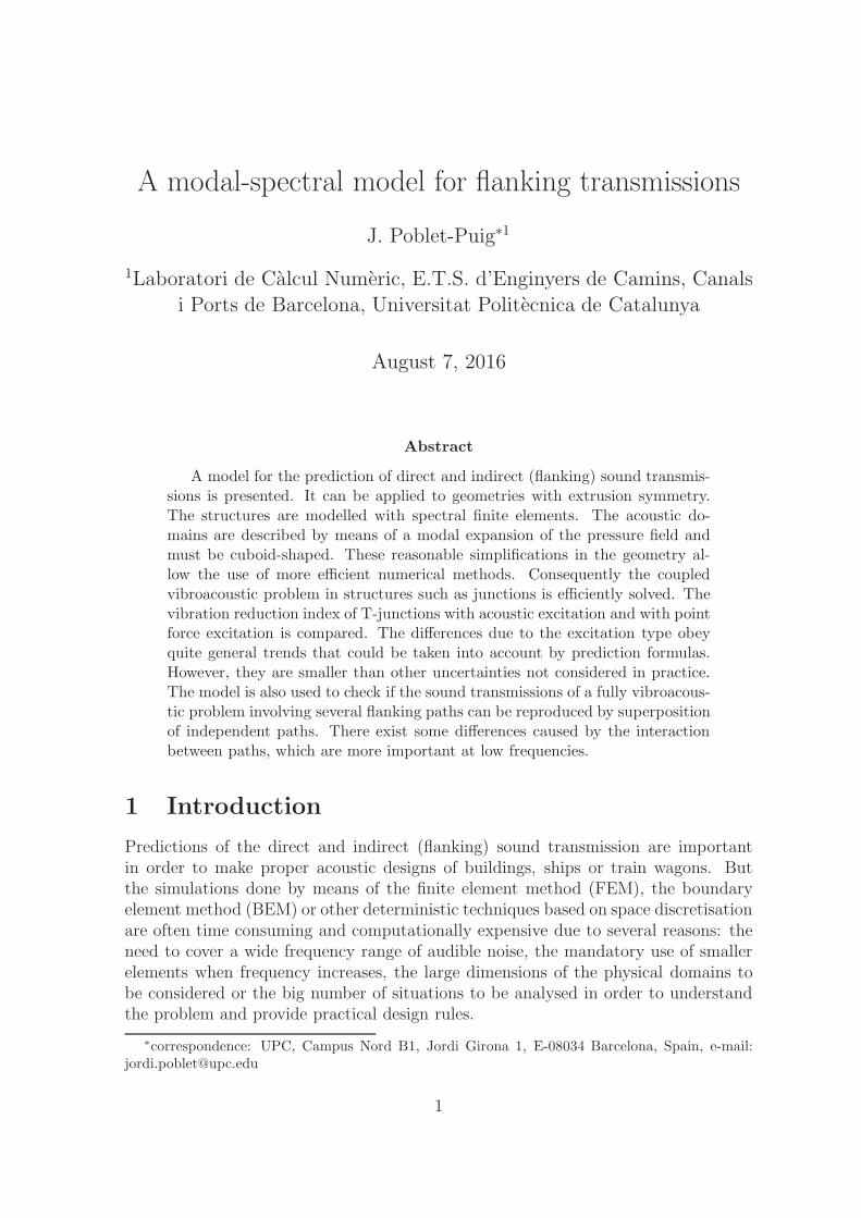
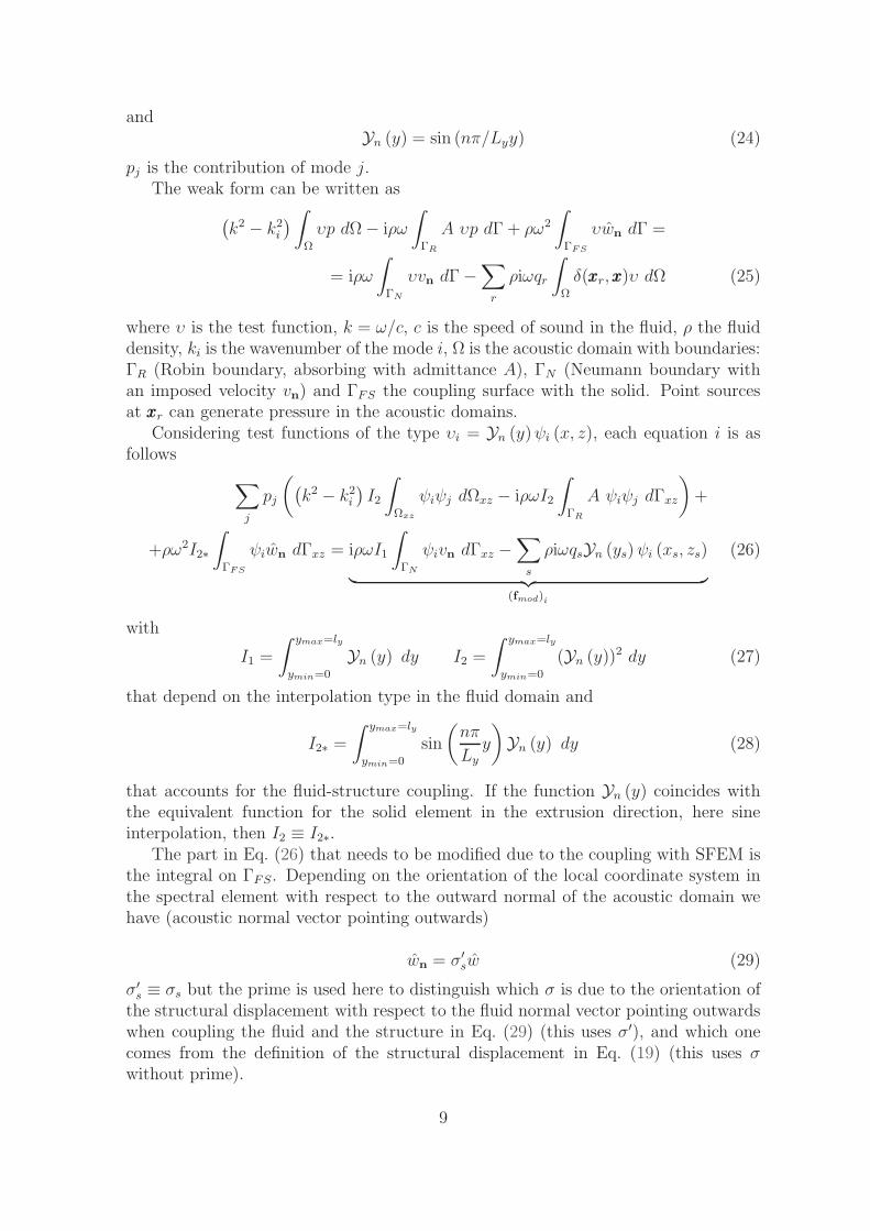
Figure 1: Sketches and notation: (a)Model of a T-shaped junction with three spectralfinite elements. Red circles indicate the used nodes (4). X, Y, Z are the global coor-dinates with displacements U, V,W . The length in the extrusion direction is Ly. Thespectral finite element with dimensions lx ×Ly has local coordinates x, y, z with localdisplacements u, v, w; (b)A single spectral element separating two acoustic domains,one at each side.

The problem is solved in the frequency-domain (steady harmonic linear elasticstructures and acoustic fluids). A pressure-displacement formulation is used. Theinteraction between the acoustic fluid and the structure is considered only in thenormal direction (as usual, the tangential friction is neglected). The implementationallows the control of the coupling and it can be decided if the contact surfaces betweenfluid and structure interact or not. If nothing is specified, fully coupled situations areconsidered (all the coincident surfaces allow fluid-structure interaction in all senses,without a priori hypotheses).

The geometries must have extrusion symmetry due to the spectral elements con-sidered and the shape of the acoustic domains. An example is the T-shaped junction

4

of Fig. 1(a) (with extrusion symmetry along the Y ≡ y direction). All the structuresanalysed are supported on a roller at the planes Y = 0 and Y = Ly where the blockeddisplacements are U = 0 and W = 0 (V is free there). It must be noted that diffusorshave not been included in the model. They are required by the standard [44] butwould complicate the formulation. The effect of the diffuse field is reproduced byproviding averaged results in the third-octave frequency bands. Moreover, when theoutput is pretended to be more general, the results obtained with different problemdimensions are averaged.

The variation along the Y direction is described by means of trigonometric func-tions (sine series are used here). It affects not only the pressure description but alsoall other room variables: excitations, wall absorption, etc. This leads to an impor-tant advantage of the method: each contribution n is solved independently from theothers. On the contrary, the use of sine series in the Y direction forces the type ofboundary conditions to be considered at Y = 0 and Y = Ly in both the structure andthe acoustic domains. For the structure, it implies that U = W = 0, which is quiteusual. However, for the acoustic domains it implies the assumption of the non veryrealistic condition of zero pressure at walls. With the positive aspect that the acousticintensity through the surfaces at Y = 0 and Y = Ly, which is required to calculate thesound reduction index, is known (null). This enforcing of boundary condition in thefluid domains is probably the most important drawback of the model but a requiredassumption in order to simplify the formulation and reduce the computational costs.These types of assumptions that sacrifice realism for the sake of better efficiency arequite usual in vibroacoustic models. Unfortunately it is a cost to pay in order toderive less complex formulations and adapt the computational costs to the availableresources. The latter is essential, otherwise the computation limitations can lead tomore undesired consequences that could be important for the final results (such as thederivation of wrong conclusions in the mid frequency range due to the small numberof problem frequencies to be averaged). The physical implications will be shown latterin Section 4. All other boundary conditions in the other zones can be imposed as itis done in spectral elements and modal expansions. In the remainder of the sectionthe formulation is presented for each harmonic ‘n’ but the subscript is omitted forclarity (except for the parameter ξn = nπ/Ly). In order to obtain the final result acombination of each uncoupled component ‘n’ must be done.

The structural elements are shells. The in-plane behaviour (local displacementsu, v) is considered as described in [9]. It is decoupled from the out-of-plane displace-ments (w). The formulation exposed here focuses the interest on the out-of-planedisplacements (bending) and the interaction with the fluid domains. The remainderof the section explains how a spectral finite element is coupled with cuboid-shapedfluid domains (see for example the single element of Fig. 1(b)). This must be, after-wards, combined with the in-plane part of the structural element, a global assemblyprocess (that is standard) and the inclusion in the global solution of the coupledproblem.

5

2.2 Fluid→structure interaction: acoustic loading of the struc-

ture

The out-of-plane displacements must be of the form

w (x, y) = w (x) sin(nπ

Lyy) (x, y) ∈ [0, lx]× [0, Ly] (1)

where x, y are the local coordinates in the element plane, lx is the element length inthe x direction, Ly is the problem/element length in y−direction. Note that due to theextrusion symmetry w is always parallel to the X−Z plane (the ‘hat’ is reserved herefor the variables reduced to the X −Z plane, when the treatment of the y−directionhas been separated).

The out-of-plane displacements are governed by the thin plate equation

∂4w

∂x4+

∂4w

∂x2∂y2+∂4w

∂y4− β2w = −q (x, y)

D(2)

with

β =

√

ρvtω2

DD =

t3E(1 + iη)

12(1− ν2). (3)

Here ρv is the volumetric density of the shell, t its thickness, ν the Poisson’s ratio, Ethe Young’s modulus, η the hysteretic damping coefficient, ω = 2πf the pulsation ofthe problem and i =

√−1 the imaginary unit. q (x, y) is the external load per unit

surface in the direction of w. If it can be expressed as

q (x, y) = q (x) sin(nπ

Lyy) (4)

then the formulation of the element is one-dimensional instead of two-dimensionaland Eq. (2) can be rewritten as

d4w

dx4− 2ξ2n

d2w

dx2+(ξ4n − β2

)w = − q

D(5)

which is an Ordinary Differential Equation (ODE) (instead of a Partial DifferentialEquation, PDE) on x. It allows solutions of the form:

w = wH + wP (6)

accounting for the homogeneous (H) and particular (P) parts. The roots of the char-acteristic polynomial are ±

√

ξ2n − β and ±√

ξ2n + β. So, the homogeneous solution isof the form

wH (x) = A1e−ik1x +B1e

−ik2x + C1e−ik1(lx−x) +D1e

−ik2(lx−x) = NSEM ·AT (7)

with k1 and k2k1 =

√

β − ξ2n k2 = −i√

β + ξ2n; (8)

and

NSEM =[e−ik1x, e−ik2x, e−ik1(lx−x), e−ik2(lx−x)

]A = [A1, B1, C1, D1] (9)

6

The key here is how to introduce the particular solution in the formulation of thespectral element with minor modifications. Similar procedures can be found in [45]where random excitation is introduced along the elements of a beam framework, in[46] where the axial and bending load in beam elements is described by means offinite element discretisation type or in [47] where spectral elements for rectangularplates subjected to turbulence excitation are formulated or [48] with an applicationfor pipes.

In the current model the excitations caused by the acoustic pressure on the contourof the cuboid-shaped domains are of the form

q (x) =

1 or 2∑

s

σs∑

j

Ps,j cos (κs,jx+ ϕs,j) (10)

with ϕs,j = L0κs,j according to Fig. 1(b) and κs,j the wavenumber of the imposedpressure on the s-side of the element. σs = ±1 accounts for the sign criterion relatedwith the local coordinates of the spectral element. In Fig. 1(b), σ1 = 1 and σ2 = −1.Ps,j is a constant that will be related latter with the modal contribution of the pressurefield.

With this excitation, the particular solution of the ODE in Eq. (5) is

wP (x) =1

D

1 or 2∑

s

∑

j

wPs,j (x) =

1

D

1 or 2∑

s

σs∑

j

Ψs,jPs,j cos (κs,jx+ ϕs,j) (11)

with

Ψs,j =1

(ξ4n − β2) + 2κ2s,jξ2n + κ4s,j

(12)

A bending dynamic stiffness matrix for the spectral element can be obtained bymeans of two steps: i) Express the boundary strengths (bending moment and shearforce) in terms of the constants A1, B1, C1 andD1 and the parameters of the particularsolution; ii) Express the constants A1, B1, C1 and D1 and the parameters of theparticular solution in terms of the nodal displacements and rotations.

The forces and moments per unit length at the nodes of the element are expressedas

Fz(x = 0, y) = D

(d3w

dx3

∣∣∣∣x=0

− ξ2n(2− ν)dw

dx

∣∣∣∣x=0

)

(13)

M(x = 0, y) = D

(

− d2w

dx2

∣∣∣∣x=0

+ ξ2nν w|x=0

)

(14)

Fz(x = lx, y) = D

(

−d3w

dx3

∣∣∣∣x=lx

+ ξ2n(2− ν)dw

dx

∣∣∣∣x=lx

)

(15)

M(x = lx, y) = D

(d2w

dx2

∣∣∣∣x=lx

− ξ2nν w|x=lx

)

(16)

Using the displacement defined in Eq. (6), the forces can be written as

fe =

Fz(x = 0, y)M(x = 0, y)Fz(x = lx, y)M(x = lx, y)

= Be

A1

B1

C1

D1

+

1 or 2∑

s

σs∑

j

Ψs,jPs,jFps,j (17)

7

with Be detailed in A and the contribution of the particular solution to the nodalforces

Fps,j =

(ξ2n(2− ν) + κ2s,j

)κs,j sin(ϕs,j)(

ξ2nν + κ2s,j)cos(ϕs,j)(

−ξ2n(2− ν)− κ2s,j)κs,j sin(κs,jlx + ϕs,j)(

−ξ2nν − κ2s,j)cos(κs,jlx + ϕs,j)

(18)

Next step is to express the nodal displacements and rotations in terms of theconstants A1, B1, C1 and D1, and the parameters related with the particular solution.A 4 × 4 system of linear equations is obtained by the evaluation of Eq. (6) at x = 0and x = lx

ue =

w|x=0dwdx

∣∣x=0

w|x=lxdwdx

∣∣x=lx

= S

A1

B1

C1

D1

+

1

D

1 or 2∑

s

σs∑

j

Ψs,jPs,j

cos(ϕs,j)−κs,j sin(ϕs,j)

cos(κs,jlx + ϕs,j)−κ sin(κs,jlx + ϕs,j)

︸ ︷︷ ︸

ups,j

(19)S, also detailed in A, is a small matrix that can be inverted in order to compute thebending dynamic stiffness matrix Kbending

e such that

Kbendinge = BeS

−1 (20)

and finally the matrix formulation at element level that accounts for possible couplingis

Kbendinge ue +

1 or 2∑

s

∑

j

σsΨs,j

(

Fps,j −

1

DKbending

e ups,j

)

︸ ︷︷ ︸

(CsFS

)·,j

Ps,j = fe (21)

with CsFS the coupling matrix that accounts for the coupling force applied to the s

side of the spectral element and fe is the vector of nodal forces defined in Eq. (17).

2.3 Structure→fluid interaction: imposed velocity on the fluid

contour

The weak form used in [31] for the acoustic domains is considered. It must be adaptedin order to account for the coupling with the spectral element. Moreover, the modesof the cuboid must be modified in order to have the same trigonometric descriptionof the pressure field in the extrusion direction as the shell spectral element. So, thepressure field is expanded in terms of modes as

p (x, y, z) = Yn (y)

nmodes∑

j=1

pjψj (x, z) (22)

with

ψj = cos

(nxjπ

lxx

)

cos

(nzjπ

lzz

)

nxj , nzj = 0, 1, 2, . . . , j, . . . (23)

8

andYn (y) = sin (nπ/Lyy) (24)

pj is the contribution of mode j.The weak form can be written as

(k2 − k2i

)∫

Ω

υp dΩ− iρω

∫

ΓR

A υp dΓ + ρω2

∫

ΓFS

υwn dΓ =

= iρω

∫

ΓN

υvn dΓ−∑

r

ρiωqr

∫

Ω

δ(xxxr,xxx)υ dΩ (25)

where υ is the test function, k = ω/c, c is the speed of sound in the fluid, ρ the fluiddensity, ki is the wavenumber of the mode i, Ω is the acoustic domain with boundaries:ΓR (Robin boundary, absorbing with admittance A), ΓN (Neumann boundary withan imposed velocity vn) and ΓFS the coupling surface with the solid. Point sourcesat xxxr can generate pressure in the acoustic domains.

Considering test functions of the type υi = Yn (y)ψi (x, z), each equation i is asfollows

∑

j

pj

((k2 − k2i

)I2

∫

Ωxz

ψiψj dΩxz − iρωI2

∫

ΓR

A ψiψj dΓxz

)

+

+ρω2I2∗

∫

ΓFS

ψiwn dΓxz = iρωI1

∫

ΓN

ψivn dΓxz −∑

s

ρiωqsYn (ys)ψi (xs, zs)

︸ ︷︷ ︸

(fmod)i

(26)

with

I1 =

∫ ymax=ly

ymin=0

Yn (y) dy I2 =

∫ ymax=ly

ymin=0

(Yn (y))2 dy (27)

that depend on the interpolation type in the fluid domain and

I2∗ =

∫ ymax=ly

ymin=0

sin

(nπ

Ly

y

)

Yn (y) dy (28)

that accounts for the fluid-structure coupling. If the function Yn (y) coincides withthe equivalent function for the solid element in the extrusion direction, here sineinterpolation, then I2 ≡ I2∗.

The part in Eq. (26) that needs to be modified due to the coupling with SFEM isthe integral on ΓFS. Depending on the orientation of the local coordinate system inthe spectral element with respect to the outward normal of the acoustic domain wehave (acoustic normal vector pointing outwards)

wn = σ′

sw (29)

σ′

s ≡ σs but the prime is used here to distinguish which σ is due to the orientation ofthe structural displacement with respect to the fluid normal vector pointing outwardswhen coupling the fluid and the structure in Eq. (29) (this uses σ′), and which onecomes from the definition of the structural displacement in Eq. (19) (this uses σwithout prime).

9

The structural displacement w of Eq. (6) can be expressed as

w = NSEM ·AT +1

D

1 or 2∑

s

σs∑

j

Ψs,jPs,j cos (κs,jx+ ϕs,j) (30)

and AT can be computed from Eq. (19) as

AT = S−1

(

ue −1

D

1 or 2∑

s

σs∑

j

Ψs,jPs,jups,j

)

(31)

Now it can be used to compute∫

ΓFSψiwn dΓxz which in practise implies the

computation of the following integrals on the structural element

∫

ΓFS

ψ(r)i wn dΓxz = σ′

r

∫

ΓFS

ψ(r)i NSEM dΓxzS

−1

︸ ︷︷ ︸

(CSF )i,·

ue

− σ′

r

1

D

1 or 2∑

s

σs∑

j

Ψs,j

∫

ΓFS

ψ(r)i NSEM dΓxzS

−1ups,j

︸ ︷︷ ︸

(C(r,s)FF

)i,j

Ps,j

+ σ′

r

1

D

1 or 2∑

s

σs∑

j

Ψs,j

∫

ΓFS

ψ(r)i cos (κs,jx+ ϕs,j) dΓxz

︸ ︷︷ ︸

(C(r,s)FF

)i,j

Ps,j

(32)

where the subscript i and superscript r in the mode ψ(r)i mean that it is the modal

function i in the acoustic domain of the side r of the structural element. The samecriterion is used for the subscript r in σ′

r which is required due to Eq. (29). (CSF )i,· isa row matrix that couples the mode i with the spectral element, and the coefficient i, jof the matrix C

(r,s)FF couples a mode i of side r with a mode j through the structural

element. The modes can be both on the same side of the element or on different sides.For this reason a spectral element with acoustic fluid in only one side needs only onematrix CFF and when the element is in contact with the fluid on both sides, it impliesfour matrices CFF : for each side of the element, interaction of the fluid with itself(C

(1,1)FF and C

(2,2)FF ) and with the fluid on the other side through the forced vibration

of the element (C(1,2)FF and C

(2,1)FF ). The calculation of the matrix coefficient is done by

considering the two indicated integrals in Eq. (32).The simple problem of two cuboid-shaped acoustic domains (rooms) separated by

a single wall (one spectral element), see Fig. 1(b) is considered in order to illustratethe way how the fluid-structure coupling is represented and the organisation of thematrices is done (creation of the coupled system of linear equations). The lower roomis denoted by the side number s = (1) and the upper room by the side number s = (2).

10

It must be also noted that Ps,j represents the amplitude of acoustic pressure onthe element side. It depends on the value of modal contribution and the evaluationof the mode shape. So, it can be written that

Ps,j = pj cos

(nzjπ

lzz

)

(33)

for the lower acoustic domain in Fig. 1(b) z = lz. And κs=1,j = nxjπ/lx. For theupper acoustic domain, z = 0. And κs=2,j = nxjπ/lx. pj is the contribution of modej for the harmonic nzj.

Similar, expressions could be used for the spectral element placed in some of theother three sides of the acoustic domain. The global system of equations is

Mmod(1) + ρω2I2C

(1,1)FF ρω2I2C

(1,2)FF ρω2I2C

(1)SF

ρω2I2C(2,1)FF Mmod

(2) + ρω2I2C(2,2)FF ρω2I2C

(2)SF

C(1)FS C

(2)FS Kbending

e

p(1)

p(2)

u

=

f(1)mod

f(2)mod

fSFEM

(34)with Mmod the modal matrix accounting for the integrals in the first row of Eq. (26),fmod the modal force vector defined in Eq. (26), fSFEM the vector of external nodalforces for the spectral element (with the same structure as the nodal force vectordefined in Eq. (17)), p the vector of modal contributions, u the vector of nodaldisplacements and rotations. The superscripts indicate the side of the element whichis equivalent for this simple case, to the acoustic domain number ((1) for the lowerand (2) for the upper).

For more complex structures, the matrices for each structural element and thecoupling matrices must be assembled by means of a standard FEM procedure. Notethat the size of this linear system of equations is smaller than the dimension of thelinear system of equations required by the solution of the same problem by means ofa FEM or FSM formulation.

3 Numerical results and analysis

The numerical model is applied to the study of the vibration and sound transmissionbetween two rooms separated by a T-shaped structure (Sections 3.1 and 3.4) or asingle wall (Sections 3.2 and 3.3), and four rooms separated by a X-shaped junction(Section 3.5). First, in Section 3.1, the results obtained by means of the modal-spectralmodel are compared with the results obtained with the finite strip method (FSM) [49].A single junction (one set of dimensions and material properties) is considered.

Section 3.2 deals with the major numerical drawback of the model. In somesituations, S is very ill-conditioned which causes poor quality of the solutions. It isillustrated with the study of the sound transmission through a single wall. A remedyis also proposed.

In Section 3.4 a parametric analysis to gain knowledge on the general behaviourof the T-junction is performed. It requires a large number of computations andconsequently any saving of time is very important. The efficiency is one of the main

11

advantages of modal-spectral model with respect to other element-based approaches(like FEM or FSM).

Finally, in Section 3.5 the assumption of path independence is checked for an X-junction. The solution of the global problem is compared with the combination ofresults obtained by simulation of all paths separately.

In all the examples shown here c = 340 m/s and ρ = 1.18 kg/m3. The real valuesof admittance A for the absorbing (Robin) boundaries are taken from Table 1.

1/Aρc 20 32.5 70α(%) 30 20 10

Table 1: Values of normalised admittance and random incidence absorption coefficientfor the Robin boundary condition (calculated as proposed in [50]).

In the T-junction and X-junction cases, each acoustic domain has two rectangularsurfaces in contact with the structure, two rectangular surfaces with null pressure(Y = 0 and Y = Ly) and two rectangular surfaces (ΓR) where an acoustic absorptioncan be imposed by means of the admittance value A. The surfaces of null pressure area consequence of the interpolation functions chosen in the extrusion direction (thatare sines, see Eqs. (1) and (24)). Null acoustic intensity passes through them.

In all the simulations the full vibroacoustic problem is solved. It means thatin-plane and out-of-plane wave motion in the structure is always possible and fullycoupling with all the acoustic domains is considered.

3.1 Comparison with the FSM

As detailed in Section 2, the proposed model has some geometrical limitations: ex-trusion symmetry and use of sine function as harmonic interpolation in this direction.FSM can exactly reproduce these limitations in order to make a fair comparison. Forthis reason, the FSM [49] is chosen in order to compare the combination of modal-spectral interpolation with an element-based approach. The treatment of the Y -direction is the same in both models while the difference relies on the X−Z plane. Itmust be noted that FSM is more flexible in the treatment of the extrusion directionbecause different interpolation functions in the fluid and the structure can be usedwithout major modifications in the formulation. As detailed above, the proposedmodel requires equal interpolation functions in the fluid and the solid parts. An ad-ditional drawback of FSM with respect to the spectral-modal model is that it stillrequires the use of a fine discretisation in the two-dimensional plane.

A single T-junction structure that separates a sending and a receiving room isconsidered. It is made of concrete (see Table 3) with a thickness in each zone of 0.1m. The total damping ηtotal = ηint + ηboundary is composed by the internal damping(ηint) plus the boundary losses considered with ηboundary = f−0.5 according to [51].

The length of the problem in the extrusion direction is Ly = 4.0 m, the sendingroom has dimensions Lx,s = 3.5 m ×Lz,s = 2.5 and the receiving room Lx,r = 4.5m ×Lz,r = 2.5. A point source (qs = 0.01 m3/s) is placed in bottom left corner ofthe sending room, separated 0.5 m from the boundaries. More precisely, it is a point

12

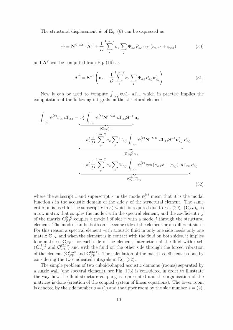
source in the X−Z plane, described by means of a triangular mesh (FSM) or a modalexpansion. In the FSM, a node of the triangular mesh is placed in the position ofthe source which is represented by a non-null term of the force vector correspondingto that node. On the contrary in the modal expansion, the force vector related toeach modal contribution is not null. It means that the spatial description of the pointsource in the X − Z plane, which is of the Dirac delta form, is done through allthe modes. Ideally, infinite modes would be required to approximate a Dirac deltafunction and the truncation of the modal base introduces some additional error inthe spatial description of the source. In addition, an element-based interpolationis more adequate than a mode-based to describe the variation of the pressure fieldaround the point source. In the Y -direction, the point sound source requires alsothe representation of a Dirac delta function. The accuracy depends on the numberof harmonics considered. Ideally, infinite sine functions should be required, which isnever the case. This number and other model parameters are shown in Table 2 foreach third-octave frequency band.

For each frequency f all modes with wavenumber

k =

√(nπ

Ly

)2

+

(nxjπ

lx

)2

+

(nzjπ

lz

)2

(35)

in the range (0, 2π(max (1.3f, f + 200))/c) have been considered. This aspectcan be of course optimised, see for example [22, 52]. However, some of the availablestrategies lose its sense here because solutions are obtained in separate harmonics.This makes in practise not so clear how to neglect the less important modes and keepthe efficiency of the implementation. On the contrary, it is an important advantagefrom the efficiency point of view to split the problem in smaller sub-problems. Eachharmonic leads to a linear system of equations with a matrix that is full but has amuch smaller dimension than FEM matrices or when the problem is considered astrue three-dimensional.

Several transmission paths are taken into account. They are enforced by allowingor not the contact between the structure and the acoustic domains. For example, inthe path 13, straight transmission, the sound is generated in the source room whichis in contact only with the zone 1 of the T-junction and not with the zone 2. Thereceiving room is in contact with the zone 3 of the T-junction and not with the zone2. The model is in the same way adapted to deal with other transmission paths.

Figs. 2 and 3 show pressure levels in each of the rooms

Lp = 10 log10

(< p2rms >

p20

)

(36)

and velocity levels in each zone of the T-shaped structure

Lv = 10 log10

(< v2rms >

v20

)

(37)

with the reference values of pressure p0 = 2× 10−5 Pa and velocity v0 = 5× 10−8m/s.< p2rms > and < v2rms > are respectively the spatial averaged pressure in a roomand the spatial averaged velocity in a zone of the structure (the zones are the entire

13

f0 (Hz) num. of harmonics ∆f (Hz) hfluid hsolid50 3 1.0 0.4 0.163 3 1.0 0.4 0.180 4 1.0 0.3 0.1100 4 2.0 0.3 0.1125 5 2.0 0.3 0.1160 6 2.0 0.2 0.1200 7 2.0 0.2 0.1250 8 3.0 0.15 0.1315 10 3.0 0.1 0.1400 12 4.0 0.1 0.1500 15 5.0 0.1 0.1630 18 6.0 0.08 0.1800 23 10.0 0.06 0.11000 28 15.0 0.05 0.11250 35 20.0 0.04 0.1

Table 2: Third-octave frequency-band values for several model parameters: f0 is thecentral frequency of the band, ‘num. of harmonics’ is the number of harmonics con-sidered (always starting from 1), ∆f is the frequency step or the separation betweenthe considered calculation frequencies, hfluid and hsolid are the element sizes used inthe fluid and solid part respectively for the FSM cross-sections.

rectangular plates shown in Fig. 1(a)). The nodal points used to make the spatialaverage are similar in both models and uniformly distributed all around the structurezone or the acoustic domain. The Figs. 2 and 3 are just representative examples ofthe results obtained for two of the paths.

In both Figs. 2 and 3 the acoustic absorption is 20%. With this value and thementioned room dimensions, the Schroeder frequency of the rooms is around 350 Hz.The simulations have also been done with acoustic absorption of 10% and 30%, leadingto similar conclusions.

The results for all of them show that both models are fully equivalent from theengineering point of view, with the difference that modal-spectral is much faster.This conclusion is valid for all the output types and zones. A difference of 0.4 dBin Fig. 3 is equivalent to a difference of 10% in the spatial averaged output. Theyare mainly caused by the different discretisation of the point source and treatment ofboundaries (absorbing and coupling). In the acoustic domains described by means ofthe modal expansion, the boundary effects are taken into account through the weakform Eq. (26). This represents just a good approximation but limited by the type ofmodes used, with null normal derivative at the boundary (for more details see [53]).

The modal behaviour is described in a very similar way for both models in Fig. 2.Only above the 250 Hz the curves start having a small random component without thedeeply pronounced peaks due to the resonances. This is coherent with the mentionedvalue of the Schroeder frequency of the rooms.

14

20.0

30.0

40.0

50.0

60.0

70.0

80.0

90.0

100.0

40

50

63

80

100

125

160

200

250

315L P

(dB

)

f (Hz)

Sending, FSM Receiving, FSM

Sending, Modal-SFEM Receiving, Modal-SFEM

(a)

15.0 20.0 25.0 30.0 35.0 40.0 45.0 50.0 55.0 60.0 65.0

40

50

63

80

100

125

160

200

250

315L v

(dB

)

f (Hz)

FSM, zone 1 Modal-SFEM, zone 1

FSM, zone 3 Modal-SFEM, zone 3

FSM, zone 2 Modal-SFEM, zone 2

(b)

Figure 2: Example of the frequency-dependent output obtained with the finite stripmethod (FSM) and the spectral-modal model (Modal-SFEM) with a room absorptionof 20%: (a) Pressure levels in sending and receiving rooms for the 12 (right angle)transmission path; (b) Velocity levels for the 13 (straight) transmission path.

3.2 The conditioning problem

The matrix S, for an undamped spectral finite element of length ℓ, is singular if thefollowing equation is satisfied

8k1k2ei(k2+k1)ℓ +

((k22 − 2k1k2 + k21

)e2i(k1+k2)ℓ

)+

+(−k22 − 2k1k2 − k21)(e2ik1ℓ + e2ik2ℓ) + (k22 − 2k1k2 + k21) = 0 (38)

This is a purely numerical phenomenon not related with any physical resonance of thestructure. It is important to note that Eq. (38) depends on the physical parametersof the structure but also on the element length. And the element length depends onthe discretisation which is independent of the structure dimensions.

15

0.01

0.1

1

10

50

63

80

100

125

160

200

250

315

400

|Lp,

FS

M -

Lp,

Mod

SF

EM

| (dB

)

f (Hz)

13 sending 13 receiving

12 sending 12 receiving

(a)

0.001

0.01

0.1

1

10

50

63

80

100

125

160

200

250

315

400

|Lv,

FS

M -

Lv,

Mod

SF

EM

| (dB

)

f (Hz)

13, zone 1 13, zone 3 13, zone 2

12, zone 1 12, zone 3 12, zone 2

(b)

Figure 3: Measure of the differences between the finite strip method and the spectral-modal model. Absolute difference of the third-octave frequency band outputs: (a)pressure levels for several transmission paths; (b) velocity levels for the 13 (straight)transmission path.

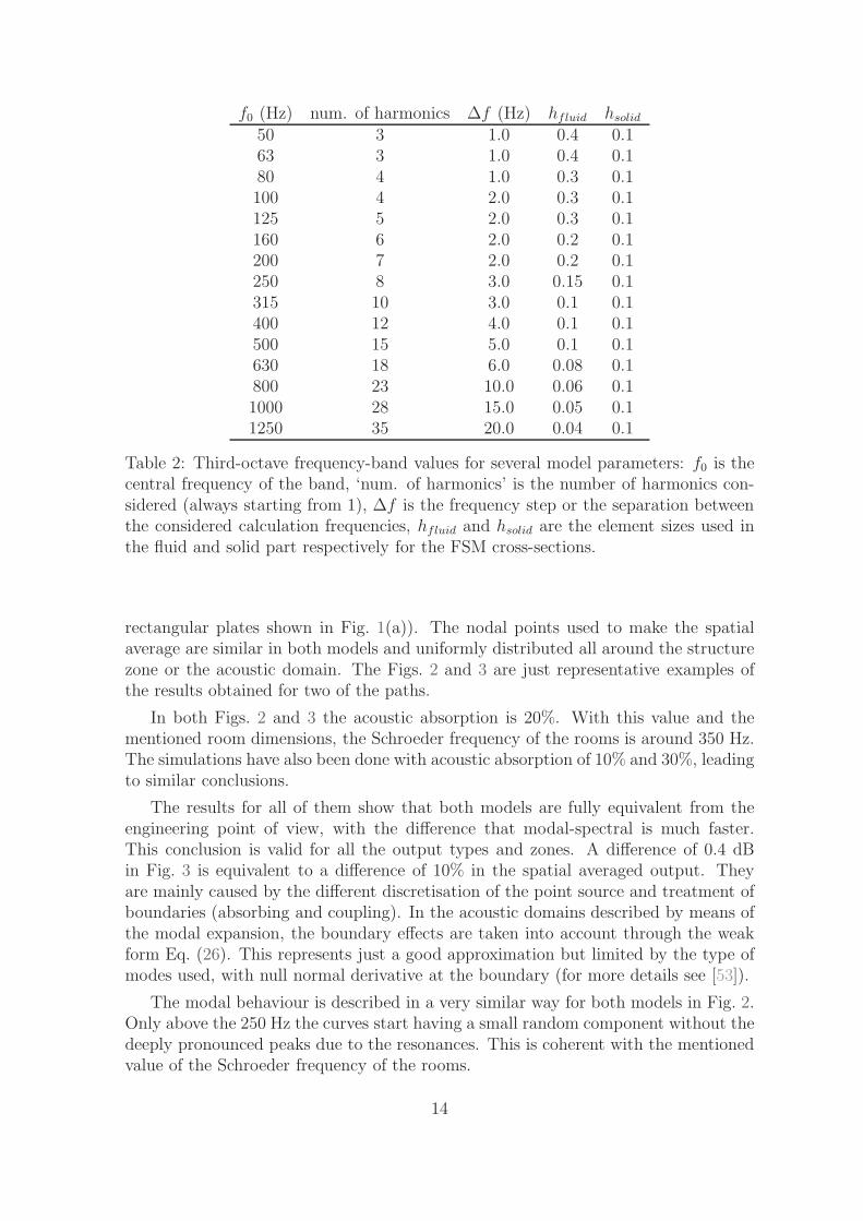
The roots of Eq. (38) can be found by successive application of the Newton-Raphson method using different first guesses that cover the whole frequency range ofinterest. It is not usual to deal with parameters that precisely satisfy this singularity.However, similar situations (lightly damped elements or frequencies that are close tothe Eq. (38) roots) can be of interest. In these cases, the matrix S−1 can be veryill-conditioned. See, for example, Fig. 4 that shows the condition number of S−1 fora 0.1 m thick spectral element made of concrete (material properties of Table 3).

The ill-conditioning of S−1 does not affect the performance of the spectral elementsfor the uncoupled structural problem. However, it can have undesirable consequencesfor the quality of the numerical solution in the coupled vibroacoustic problem pre-sented here. The propagation of numerical errors is mainly important at low frequen-cies and for those situations when some spectral element is coupled to the fluid inboth sides. It excludes the 12 and 13 transmissions for the T-junction of Section 3.1but not a simple case of sound transmission through a single wall.

The remedy adopted here in order to overcome this numerical drawback is asfollows:

• Make the discretisation of the structure by using the largest spectral elements.In the case of a T-junction, three spectral elements is enough. This saves somecomputation time.

• Compute all the spurious frequencies as roots of Eq. (38) in all the frequencyrange of interest and for all the harmonics involved in the solution of the problem.

16

100

101

102

103

104

105

50

63

80

100

125

160

200

250

315

400

500

630

800

1000

cond

(S-1

)

f (Hz)

n=1 n=2 n=3

(a)

100

101

102

103

104

105

106

50

63

80

100

125

160

200

250

315

400

500

630

800

1000

cond

(S-1

)

f (Hz)

n=1 n=2 n=3

(b)

Figure 4: Condition number of the matrix S−1 for several harmonics n in an spectralelement made of concrete: (a) 2.5 m length; (b) 1.25 m length.

• For those situations around the spurious frequencies use an alternative mesh.This mesh can be as simple as divide the problematic spectral element by two.It must be checked that no problems related with the modified discretisationappear around the studied frequency. Fig. 4 shows how the condition numberof S−1 varies when modifying the element length. It seems reasonable to definesecurity bands of 10 Hz around the spurious frequencies to activate this remedy(if the calculation frequency falls inside this security band, the probability ofobtaining a numerical result affected by the ill-condition problem is importantand the remedy is activated). This band can be smaller at high frequencies.

It must be noted that not all the spurious frequencies cause the propagation of numer-ical errors. But no consistent procedure to determine which of them are problematichas been found.

A model problem is built by considering all the material and geometrical param-eters used in Section 3.1 but replacing the T-junction with a single leaf on zone 2.This allows the discussion to be focused in a 2.5 m length element. However, the samecomments are valid for the T-junction when the path 33 is analysed or all possiblefluid-structure contact surfaces activated. The relevant aspect is to have some of thespectral elements with fluids on both sides.

The results in Fig. 5 illustrate the anomalous behaviour for the sound transmissionthrough a single wall and how the numerical difficulties have been overcome. Threenumerical models of the same physical problem are compared: A) FSM; B) modal-spectral model where the wall is described by means of only one element; C) modal-spectral model where the wall is described by means of an alternative discretisationof two elements (1.25 m length each) around the spurious frequencies of model B.

Away from the spurious frequencies of the second model (shown by crosses) all the

17

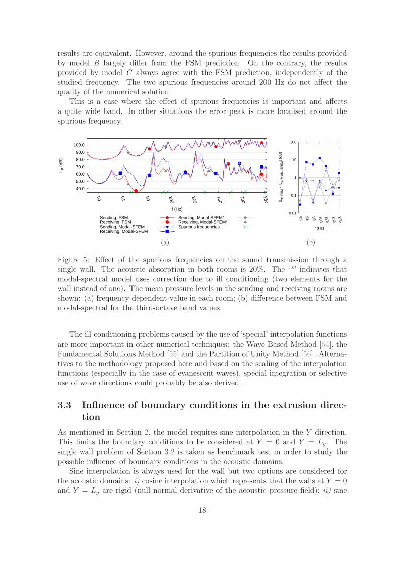
results are equivalent. However, around the spurious frequencies the results providedby model B largely differ from the FSM prediction. On the contrary, the resultsprovided by model C always agree with the FSM prediction, independently of thestudied frequency. The two spurious frequencies around 200 Hz do not affect thequality of the numerical solution.

This is a case where the effect of spurious frequencies is important and affectsa quite wide band. In other situations the error peak is more localised around thespurious frequency.

40.0

50.0

60.0

70.0

80.0

90.0

100.0

50

63

80

100

125

160

200

250

L P (

dB)

f (Hz)

Sending, FSM Receiving, FSM Sending, Modal-SFEM Receiving, Modal-SFEM

Sending, Modal-SFEM* Receiving, Modal-SFEM* Spurious frequencies

(a)

0.01

0.1

1

10

100

50

63

80 100 125

160 200

|Lp,

FS

M -

Lp,

Mod

al-S

FE

M| (

dB)

f (Hz)

(b)

Figure 5: Effect of the spurious frequencies on the sound transmission through asingle wall. The acoustic absorption in both rooms is 20%. The ‘*’ indicates thatmodal-spectral model uses correction due to ill conditioning (two elements for thewall instead of one). The mean pressure levels in the sending and receiving rooms areshown: (a) frequency-dependent value in each room; (b) difference between FSM andmodal-spectral for the third-octave band values.

The ill-conditioning problems caused by the use of ‘special’ interpolation functionsare more important in other numerical techniques: the Wave Based Method [54], theFundamental Solutions Method [55] and the Partition of Unity Method [56]. Alterna-tives to the methodology proposed here and based on the scaling of the interpolationfunctions (especially in the case of evanescent waves), special integration or selectiveuse of wave directions could probably be also derived.

3.3 Influence of boundary conditions in the extrusion direc-

tion

As mentioned in Section 2, the model requires sine interpolation in the Y direction.This limits the boundary conditions to be considered at Y = 0 and Y = Ly. Thesingle wall problem of Section 3.2 is taken as benchmark test in order to study thepossible influence of boundary conditions in the acoustic domains.

Sine interpolation is always used for the wall but two options are considered forthe acoustic domains: i) cosine interpolation which represents that the walls at Y = 0and Y = Ly are rigid (null normal derivative of the acoustic pressure field); ii) sine

18

interpolation that implies the assumption of zero pressure at Y = 0 and Y = Ly.The first case is solved by means of the FSM [49] and with a fully modal approachwhere both the acoustic domains and the plate are described by means of a modalexpansion as done in [19, 22]. This modal-modal model allows the simulation ofhigher frequencies than the FSM. For the second case, both models are adapted inorder to use sine interpolation in the Y direction. This allows a comparison with theModal-SFEM model presented here.

60.0

70.0

80.0

90.0

100.0

110.0

50

63

80

100 125

160 200 250 315

400 500 630

800 1000

L P (

dB)

f (Hz)

S, FSM cosS, Modal cosS, FSM sinS, Modal sinS, Modal-SFEM*

R, FSM cosR, Modal cosR, FSM sinR, Modal sinR, Modal-SFEM*

(a)

50.0

60.0

70.0 50

63

80

100 125

160 200 250 315

400 500 630

800 1000

L v (

dB)

f (Hz)

FSM cosModal cos

FSM sinModal sin

Modal-SFEM*

(b)

Figure 6: Sound transmission through a single wall. Influence of boundary conditions,sine or cosine interpolation is used in the Y direction of the acoustic domains. Thelabels for the models are as follows: ‘FSM cos’ and ‘FSM sin’ denote the finite stripmethod with cosine or sine interpolation in the Y direction respectively; ‘Modal cos’and ‘Modal sin’ is used for the fully modal expansion (acoustic and solid domains)with cosine or sine interpolation in the Y direction respectively; ‘Modal-SFEM*’ isthe Modal-SFEM model presented here with the correction mentioned in Section 3.2.(a)Sound pressure level (The labels ‘S’ and ‘R’ mean sending and receiving roomrespectively); (b) Velocity level.

Fig. 6 illustrates the effect that the modification of the acoustic boundary condi-tions have on the final outputs. As expected, this is more important at low frequencies.The pressure field of the modes with small n = 0, 1, 2, . . . is very different (the spatialdistribution of pressure in the Y direction differs a lot).

The differences are less important at mid frequencies and larger values of n whereeven if the pressure field in the Y direction can still be different, the spatial wavenum-ber is similar and we have different pressure waves that produce a similar excitationon the structure.

19

3.4 Parametric T-shaped junction

The main advantage of the modal-spectral model is the efficiency. This is illustratedhere with the parametric analysis of a T-shaped junction in the framework of a vibroa-coustic problem. Recent researches [8, 7, 9] are trying to develop simple but generaldesign rules for the vibration behaviour of some common structural components. Alarge number of simulations is required in order to make the final prediction formulasindependent of the less influencing parameters.

The remainder of the section, is an illustration of how the modal-spectral modelcan be a useful tool to perform this type of massive vibroacoustic simulations not onlyat low-frequencies but also at mid-frequencies.

A population of T-junctions is considered. They are generated with the materialparameters of Table 3 considering: i) homogeneous junctions made of concrete, aer-ated concrete blocks and calcium silicate blocks; ii) junctions made of concrete in thezone 2 and other material in zones 1 and 3 (aerated concrete blocks, bricks or denseaggregate blocks). The thicknesses of each zone can be 0.1, 0.2 and 0.3 m with atotal of 9 possible combinations (zones 1 and 3 have always the same thickness). Arange of mass ratios according to common junctions found in heavyweight buildingsis covered.

The dimensions of the T-junction and rooms are: Ly = 4.0, 5.0 or 6.0 m in theextrusion direction, Lx = 3.5, 4.5 or 5.5 m and Lz = 2.5 m for both sending andreceiving rooms. It makes a total of 27 sets of T-junctions and rooms with differentdimensions. The result for each junction type (thicknesses and material combination)is provided as the average of these 27 sets of dimensions with the standard deviation.The goal is to obtain a general trend, independent of the problem dimensions.

The main output of interest is the vibration reduction index as defined in [2, 5, 9]

Kij = Dν,ij + 10 log10

(ℓij√aiaj

)

with ai =2.2πSi

cTi

√

freff

(39)

where Dν,ij is the direction averaged vibration level difference, ℓij is the length of thejunction, ai is the equivalent absorption length of the plate i, Si its surface, c the speedof sound in the air, fref = 1000 Hz is a reference frequency and Ti the reverberationtime of the wall i that can be calculated as Ti = 2.2/ (ηtotalf). ηtotal = ηint + ηboundaryis the total loss factor that accounts for the internal damping (ηint) and the boundarylosses, considered as ηboundary = f−0.5 according to [51].

For the case of point force excitation, an alternative to compute the spatial averageof the velocity level Lv is considered by excluding the zone of 1 m around the pointforce. This option is indicated in the figures with the symbol ‘*’. This spatial averagetries to neglect the effect caused by the near field around the force application zoneand is more coherent with the measurement procedure described in [57].

The coupling surfaces are modified as explained in Section 3.1 in order to allowonly one possible transmission path. Ki,j is direction averaged. In practise for eachjunction two situations are considered, sending room on the left and vice-versa. Inevery situation a point (in the X − Z plane) source is placed in bottom corner, awayfrom zone 2 and separated 0.5 m from the walls. The main difference with previousworks[9] is that Ki,j is now obtained by means of acoustic excitation instead of point

20

forces. The effect of the receiving room on the structure can probably be neglected formost of the frequencies if just the Ki,j with acoustic excitation needs to be computed.However, at some resonances of the receiving room this hypothesis can be false. Itis not easy to determine a priori when this can happen. For this reason and thanksto the versatility of the implementation, it is easier and more realistic to consider thereceiving room in all the cases.

The mass ratio between the surface density of the orthogonal structural zone andthe current one (see [2]) is used as the parameter that characterises the junction.

Material ρv (kg/m3) ν E (Pa) ηintConcrete 2200 0.2 3.05 · 1010 0.005Aerated concrete blocks (1) 400 0.2 1.39 · 109 0.0125Aerated concrete blocks (2) 800 0.2 2.77 · 109 0.0125Dense aggregate blocks 2000 0.2 1.97 · 1010 0.01Bricks 1750 0.2 1.22 · 1010 0.01Calcium silicate blocks 1800 0.2 1.08 · 1010 0.01

Table 3: Material properties (frequency independent) of the parametric analysis.Same materials as [8] have been considered.

For each set of 27 junctions, two single values of Ki,j are obtained. One is forthe low frequencies (average of third-octave frequency bands between 50 Hz and 200Hz) and the other for mid frequencies (average between 250 Hz and 1000 Hz). Thestandard deviation of these 27 junctions is also provided. Even if performing singlesimulations up to 2000 Hz with the mentioned problem dimensions is reasonable, toobtain a high-frequency value (up to 4000 Hz) from a parametric analysis is currentlyout of the possibilities of the presented model.

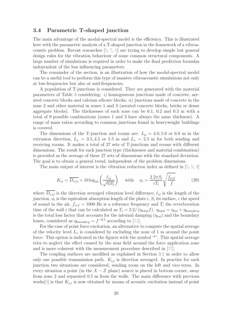
The low-frequency results are shown in Fig. 7 for the right-angle transmission (12)and Fig. 8 for the straight transmission (13). Apart from the Ki,j values obtained withthe vibroacoustic modal-spectral simulations (Modal SFEM), the following data is alsoplotted: the sameKi,j values obtained with the FSMmodel (for some of the junctions);the Ki,j for the same junctions but considering point force excitation (average of threedifferent positions) using the SFEM model described in [9] ,considering spatial averageall around the excited plate (SFEM Point Force) or excluding the zone around theforce (SFEM Point Force*); the prediction formula proposed in the annex of the EN-12354 regulation [2]; the simplified formula obtained in [8] by statistical regression ofa cloud of Ki,j data generated by means of a wave approach model (Hopkins).

The predictions done with FSM and modal-spectral are very similar. However,FSM takes much more time. In the low-frequency range, Ki,j values obtained withacoustic excitation are in most of the cases 1 or 2 dB larger than their equivalentobtained with point force excitation. However, this trend seems to be inverted forthe junctions with the largest mass ratio. In both cases, right angle and straighttransmission, the general trend shows the same differences with EN-12354 that aredescribed in [8] or [9]. They are more relevant for the right angle transmission injunctions with a mass ratio different than 1.

21

The modification in the spatial average of the results obtained with point forceexcitation causes a reduction of the Ki,j values in all cases: low and mid frequencies,straight and right angle transmission. This is explained because the exclusion of thezone around the force application diminished the velocity level in the source plate.The velocity level in the other plates remain the same and consequently the vibrationlevel difference also diminishes. This variation is more important at low frequencies.In the mid frequency range, the values with the modified spatial average are closer tothe values obtained with acoustic excitation. This makes sense because the exclusionof the near field produces a more uniform vibration field which is the case of acousticexcitation.

-5

0

5

10

15

20

0.1 1 10

Kij

(dB

)

m⊥ /mi

EN-12354 Hopkins (0.33< m⊥ /mi <16.59) Modal SFEM

FSM SFEM Point Force SFEM Point Force*

(a)

0

0.5

1

1.5

2

0.1 1 10

σ Kij (

dB)

m⊥ /mi

(b)

Figure 7: Low-frequency averaged vibration reduction index for a T-shaped junction,right angle transmission (12): (a) Vibration reduction index for each mass ratio value;(b) Standard deviation of each data point due to the change of junction and roomdimensions.

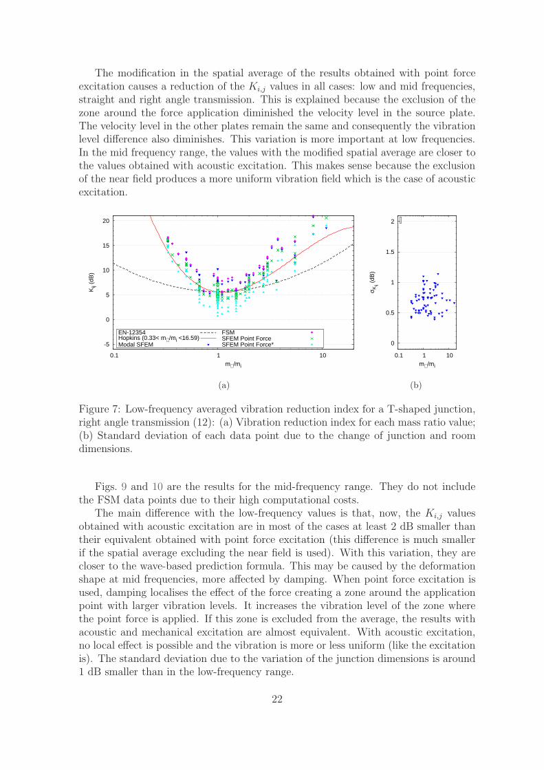
Figs. 9 and 10 are the results for the mid-frequency range. They do not includethe FSM data points due to their high computational costs.

The main difference with the low-frequency values is that, now, the Ki,j valuesobtained with acoustic excitation are in most of the cases at least 2 dB smaller thantheir equivalent obtained with point force excitation (this difference is much smallerif the spatial average excluding the near field is used). With this variation, they arecloser to the wave-based prediction formula. This may be caused by the deformationshape at mid frequencies, more affected by damping. When point force excitation isused, damping localises the effect of the force creating a zone around the applicationpoint with larger vibration levels. It increases the vibration level of the zone wherethe point force is applied. If this zone is excluded from the average, the results withacoustic and mechanical excitation are almost equivalent. With acoustic excitation,no local effect is possible and the vibration is more or less uniform (like the excitationis). The standard deviation due to the variation of the junction dimensions is around1 dB smaller than in the low-frequency range.

22

0

10

20

30

40

0.1 1 10

Kij

(dB

)

m⊥ /mi

EN-12354 Modal SFEM

FSM SFEM Point Force

SFEM Point Force*

(a)

0

0.5

1

1.5

2

0.1 1 10

σ Kij (

dB)

m⊥ /mi

(b)

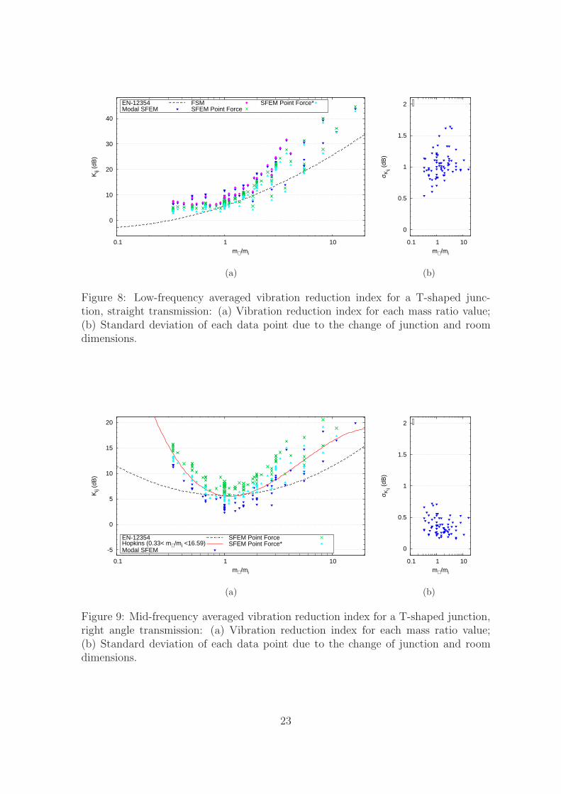
Figure 8: Low-frequency averaged vibration reduction index for a T-shaped junc-tion, straight transmission: (a) Vibration reduction index for each mass ratio value;(b) Standard deviation of each data point due to the change of junction and roomdimensions.

-5

0

5

10

15

20

0.1 1 10

Kij

(dB

)

m⊥ /mi

EN-12354 Hopkins (0.33< m⊥ /mi <16.59) Modal SFEM

SFEM Point Force SFEM Point Force*

(a)

0

0.5

1

1.5

2

0.1 1 10

σ Kij (

dB)

m⊥ /mi

(b)

Figure 9: Mid-frequency averaged vibration reduction index for a T-shaped junction,right angle transmission: (a) Vibration reduction index for each mass ratio value;(b) Standard deviation of each data point due to the change of junction and roomdimensions.

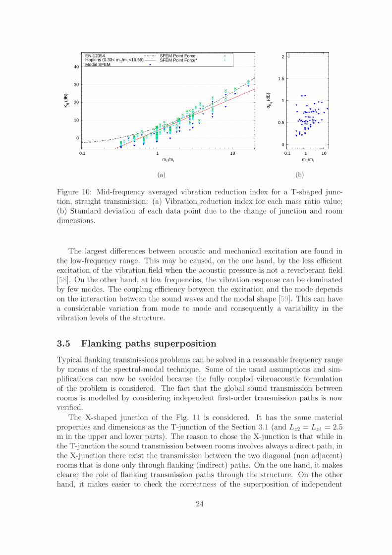
23

0

10

20

30

40

0.1 1 10

Kij

(dB

)

m⊥ /mi

EN-12354 Hopkins (0.33< m⊥ /mi <16.59) Modal SFEM

SFEM Point Force SFEM Point Force*

(a)

0

0.5

1

1.5

2

0.1 1 10

σ Kij (

dB)

m⊥ /mi

(b)

Figure 10: Mid-frequency averaged vibration reduction index for a T-shaped junc-tion, straight transmission: (a) Vibration reduction index for each mass ratio value;(b) Standard deviation of each data point due to the change of junction and roomdimensions.

The largest differences between acoustic and mechanical excitation are found inthe low-frequency range. This may be caused, on the one hand, by the less efficientexcitation of the vibration field when the acoustic pressure is not a reverberant field[58]. On the other hand, at low frequencies, the vibration response can be dominatedby few modes. The coupling efficiency between the excitation and the mode dependson the interaction between the sound waves and the modal shape [59]. This can havea considerable variation from mode to mode and consequently a variability in thevibration levels of the structure.

3.5 Flanking paths superposition

Typical flanking transmissions problems can be solved in a reasonable frequency rangeby means of the spectral-modal technique. Some of the usual assumptions and sim-plifications can now be avoided because the fully coupled vibroacoustic formulationof the problem is considered. The fact that the global sound transmission betweenrooms is modelled by considering independent first-order transmission paths is nowverified.

The X-shaped junction of the Fig. 11 is considered. It has the same materialproperties and dimensions as the T-junction of the Section 3.1 (and Lz2 = Lz4 = 2.5m in the upper and lower parts). The reason to chose the X-junction is that while inthe T-junction the sound transmission between rooms involves always a direct path, inthe X-junction there exist the transmission between the two diagonal (non adjacent)rooms that is done only through flanking (indirect) paths. On the one hand, it makesclearer the role of flanking transmission paths through the structure. On the otherhand, it makes easier to check the correctness of the superposition of independent

24

flanking paths.

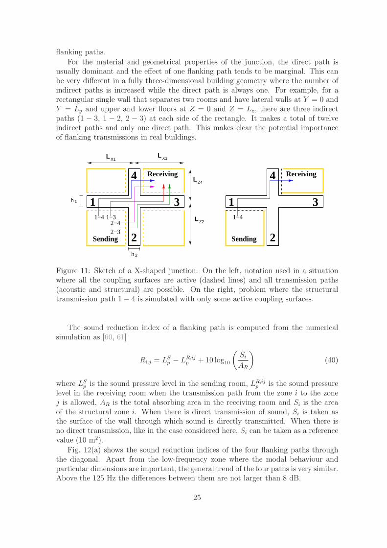
For the material and geometrical properties of the junction, the direct path isusually dominant and the effect of one flanking path tends to be marginal. This canbe very different in a fully three-dimensional building geometry where the number ofindirect paths is increased while the direct path is always one. For example, for arectangular single wall that separates two rooms and have lateral walls at Y = 0 andY = Ly and upper and lower floors at Z = 0 and Z = Lz, there are three indirectpaths (1 − 3, 1 − 2, 2 − 3) at each side of the rectangle. It makes a total of twelveindirect paths and only one direct path. This makes clear the potential importanceof flanking transmissions in real buildings.

LZ4

LZ2

h2

LX1LX3

h1

2

4

31

Receiving

1−4

Sending

1−32−4

2−32

4

31

Receiving

1−4

Sending

Figure 11: Sketch of a X-shaped junction. On the left, notation used in a situationwhere all the coupling surfaces are active (dashed lines) and all transmission paths(acoustic and structural) are possible. On the right, problem where the structuraltransmission path 1− 4 is simulated with only some active coupling surfaces.

The sound reduction index of a flanking path is computed from the numericalsimulation as [60, 61]

Ri,j = LSp − LR,ij

p + 10 log10

(Si

AR

)

(40)

where LSp is the sound pressure level in the sending room, LR,ij

p is the sound pressurelevel in the receiving room when the transmission path from the zone i to the zonej is allowed, AR is the total absorbing area in the receiving room and Si is the areaof the structural zone i. When there is direct transmission of sound, Si is taken asthe surface of the wall through which sound is directly transmitted. When there isno direct transmission, like in the case considered here, Si can be taken as a referencevalue (10 m2).

Fig. 12(a) shows the sound reduction indices of the four flanking paths throughthe diagonal. Apart from the low-frequency zone where the modal behaviour andparticular dimensions are important, the general trend of the four paths is very similar.Above the 125 Hz the differences between them are not larger than 8 dB.

25

35.0

40.0

45.0

50.0

55.0

60.0

65.0

50

63

80

100 125

160 200 250 315

400 500 630

800 1000

R (

dB)

f (Hz)

1->3 1->4 2->3 2->4

(a)

35.0

40.0

45.0

50.0

55.0

60.0

65.0

50

63

80

100 125

160 200 250 315

400 500 630

800 1000

R (

dB)

f (Hz)

Indep. Struct. All

(b)

Figure 12: Flanking transmissions through a X-shaped junction: (a)Sound reductionindex (R) of each flanking path through the junction ; (b) Comparison between theoverall sound reduction index considering that each indirect flanking path is indepen-dent (Indep.), the result when all the structural paths are active at the same time(Struct.), and when all paths (structural and acoustic) are active (All).

The global sound reduction index, taking into account the effect of all the flankingpaths is computed as

Rtotali,j = 10 log10

(N∑

i=1

Si

)

− 10 log10

(N∑

i=1

Si10−Ri,j/10

)

(41)

where N is the number of paths.Fig. 12(b) shows the global sound reduction index computed in three different

ways: i)‘Indep.’: by superposition according to Eq. (41) of all possible transmis-sion paths, each of them is the result of an individual simulation where the interfaceconditions between fluid and structure has been properly adapted (see Fig. 11 thatillustrates the flanking path 1−4 with only two coupling surfaces: sending room - zone1 and receiving room - zone 4); ii) ‘Struct.’: by considering active all possible flankingpaths through the X-junction at the same time but not the airborne paths throughcontiguous rooms (only the sending and receiving rooms are modelled); iii)‘All’: con-sidering the whole problem involving four rooms and all possible transmission paths(acoustic and structural).

A first aspect to be noted is that curves ‘Struct.’ and ‘All’ are quite similar.This means that flanking paths through the structure are dominant with respect tothe airborne paths between contiguous rooms in the sound transmission through thediagonal. This is not the case in the transmission between adjacent rooms (i.e. in aT-junction) where the airborne (direct) path is clearly dominant. But now, this is asecond order path because it needs to pass through two walls (left to right and bottomto top). It drastically penalises the airborne transmission between diagonal rooms.

26

Except for the low-frequency bands (below 160 Hz), the difference between the‘Struct.’ and ‘Indep’ curves are not very large but it still exists. It means that thesuperposition of paths is a quite good approximation but not exact. Some interactionbetween the paths should exist. This observation is based on a meaningful but singleexample. Most probably a systematic analysis would lead to a more solid conclusionregarding the path superposition.

4 Discussion

The results presented in Section 3 illustrate the potentialities and drawbacks of theproposed model. Section 3.1 shows that it is in practice equivalent to a more versatilemethod based on polynomial interpolation (i.e. FSM). This is a very positive aspect,which in fact was the main goal of the research. Some of the critical aspects as wellas possible improvements and future developments are discussed next.

4.1 Computational efficiency

The formulation of this alternative method makes sense only if the final implementa-tion is more efficient than standard approaches such as FEM or BEM, which is thecase. The advantages (in terms of computational cost reduction) of using a modalexpansion technique with respect to FEM were studied in [53](Section 5.3) for the caseof a single wall modelled with structural FEM elements that separates two cuboid-shaped acoustic domains described by means of a modal expansion, and in [31] for thecase of rooms connected through holes, slits or openings. In both cases the advantagesof using a modal expansion was clear and expressed in terms of memory requirements,number of degrees of freedom and number of operations. The modal expansion affectsto the acoustic part of the problem (rooms) and this advantage is inherited here.

What is improved here is the cost of discretisation of the structure (wall or junc-tion). In [53] it was done by means of finite elements. Even if the use of FEM for thestructure is a much smaller penalty than the use of FEM for the rooms, the cost ofstructural FEM can still be important. Especially if it is compared with the cost of aproperly optimised modal description of the rooms. Now, the structural part of theproblem is solved with almost marginal costs thanks to the use of spectral elements.For a single wall (one element) it represents eight unknowns (four per node) and for aT-shaped structure three spectral elements and 16 unknowns. And all these is beforethe elimination of the imposed or blocked displacements. So, it can be said that evenif the structural matrices are full in the SFEM the costs associated to the structuralpart of the problem become almost null.

The matrices lose any specific structure but are very small. The ones associatedwith the structural part and the coupling are full and those associated with the modalexpansion can be diagonal or banded (depending of the treatment of the surfaces withabsorption, see the details in [53]). For this reason, a direct solver for full matrices isused here.

The costs associated with the Y direction are equivalent to those described for theFSM in [49]. The convergence analyses presented there, are valid here because the Y

27

direction is also described by means of trigonometric functions. The most importantaspect is the use of the same functions for the structure and acoustic domains thatallows the solution of the problem by means of decoupled blocks. This is an importantissue from the computational point of view and also from the modelling side (as shownin Section 3.3).

4.2 Weak coupling

Another aspect to be considered is the improvement of the modal expansion usedfor the acoustic domains with some technique more oriented to the vibroacousticproblems. In the current form, the model is conceived for situations of weak couplingas it is the transmission of sound through walls separating air rooms. This limitationis mainly caused by the use of normal modes (in vacuo, see Eq. (23) afterwards) andthe lack of normal velocity in the acoustic field but not due to the solution procedure(which is fully coupled). However, this modal expansion is the simplest allowing ananalytical treatment of the coupling and has been largely used [62]. Their drawbackswhen used for coupled problems (heavy loaded structures or dense fluids) with non-null normal velocity at the fluid boundary are quite well know and some remedies havebeen proposed. A physical-oriented a priori criterion to select the most importantmodes is used in [52]. A pseudo-static correction of the large numerical errors causedby the truncation of the modal base in strongly coupled problems is proposed in [63].Another technique that combines a pre-selection of modes and double enrichment ofthe solutions with information from the coupling forces and final residuals is presentedin [64] where an interesting comparison with existing methods is done. The mitigationof truncation errors can also be done in the post-processing stages [65].

The ideas and formulation exposed here could be adapted to account for some ofthe techniques mentioned above. This could be useful to extend the spectral-modalmodel presented here to strongly coupled problems (i.e. with heavier fluids). In anyof the cases, normal modes are valid for a wide range of situations of interest.

5 Conclusions

The main conclusions of the research are summarised here below:

1. A spectral(structure) and modal (acoustic) model has been developed. The mainfeature of the formulation is the coupling between both methodologies. Theresults show a good agreement with the FSM. Moreover, the final model is moreefficient (than FSM or three-dimensional FEM) as a result of the combinationof more efficient techniques and simplifications of the geometry.

2. Poor quality of the numerical solution around some spurious frequencies is ob-served. The cause is the ill-conditioning of the matrix S. It is mainly importantwhen some spectral element contacts modal acoustic domains at both sides. Thisdrawback can be overcome by using a slightly different discretisation where thelength of the problematic spectral elements is changed.

28

3. A first application to the study of sound and vibration transmission through aT-junction is done. Some differences in the vibration reduction index computedwith point force excitation and with acoustic excitation are observed. Theyare more important at low frequencies where acoustic excitation systematicallyprovides larger Ki,j values. These differences are less important at mid frequen-cies especially if spatial average that excludes the zone around the point forceexcitation is considered.

4. The model has also been used to check the hypothesis of flanking path inde-pendence. The analysis of a X-shaped junction reveals that some differencesbetween individual path superposition and the global problem exist. They aremore important at low frequencies.

A SFEM matrices related with bending

S =

1 1 e−ik1lx e−ik2lx

−ik1 −ik2 ik1e−ik1lx ik2e

−ik2lx

e−ik1lx e−ik2lx 1 1−ik1e

−ik1lx −ik2e−ik2lx ik1 ik2

(42)

Be

D=

(γn + k21) ik1 (γn + k22) ik2 (−γn − k21) ik1e1 (−γn − k22) ik2e2γ′n + k21 γ′n + k22 (γ′n + k21) e1 (γ′n + k22) e2

−(γn + k21)ik1e1 −(γn + k22)ik2e2 (γn + k21)ik1 (γn + k22)ik2− (γ′n + k21) e1 − (γ′n + k22) e2 − (γ′n + k21) − (γ′n + k22)

(43)with γn = (2− ν)ξ2n, γ

′

n = νξ2n, e1 = e−ik1lx and e2 = e−ik2lx .

Acknowledgements

Free software has been used [66]. LaCaN research group is grateful for the sponsor-ship/funding received from Generalitat de Catalunya (Grant number 2014-SGR-1471).

References

[1] S. Schoenwald. Flanking sound transmission through lightweight framed doubleleaf walls–Prediction using statistical energy analysis. PhD thesis, 2008.

[2] EN-12354. Building Acoustics: Estimation of the acoustic performance of build-ings from the performance of elements. (Acoustique du batiment: Calcul de laperformance acustique des batiments a partir de la performance des elements).Technical Report 1–4, 1999-2000.

[3] E. Gerretsen. Calculation of the sound transmission between dwellings by parti-tions and flanking structures. Appl. Acoust., 12(6):413–433, 1979.

29

[4] E. Gerretsen. Calculation of airborne and impact sound insulation beteendwellings. Appl. Acoust., 19(4):245–264, 1986.

[5] Ch. Crispin, B. Ingelaere, M. Van Damme, and D. Wuyts. The vibration reduc-tion index Kij: Laboratory measurements for rigid junctions and for junctionswith flexible interlayers. J. Building Acoustics, 13(2):99–112, 2006.

[6] Ch. Crispin, M. Mertens, B. Blasco, B. Ingelaere, M. Van Damme, and D. Wuyts.The vibration reduction index Kij:laboratory measurements versus predictionsEN 12354-1 (2000). In The 33rd international congress and exposition on noisecontrol engineering, Prague, 2004.

[7] Ch. Crispin, L. De Geetere, and B. Ingelaere. Extensions of EN 12354 vibrationreduction index expressions by means of FEM calculations. In Inter-Noise andNoise-con Congress and Conference Proceedings, volume 249, pages 5859–5868.Institute of Noise Control Engineering, 2014.

[8] C Hopkins. Determination of vibration reduction indices using wave theory forjunctions in heavyweight buildings. Acta Acust. United Acust., 100(6):1056–1066,2014.

[9] J. Poblet-Puig and C. Guigou-Carter. Using spectral finite elements for para-metric analysis of the vibration reduction index of heavy junctions oriented toflanking transmissions and EN-12354 prediction method. Appl. Acoust., 99:8–23,2015.

[10] A. Dijckmans. Structure-borne sound transmission across junctions of finite singleand double walls. In INTER-NOISE and NOISE-CON Congress and ConferenceProceedings, volume 250, pages 2731–2742. Institute of Noise Control Engineer-ing, 2015.

[11] A. Dijckmans. Vibration transmission across junctions of double walls usingthe wave approach and statistical energy analysis. Acta Acust. United Acust.,102(3):488–502, 2016.

[12] J.F. Doyle. Wave propagation in structures: spectral analysis using fast discretefourier transforms. Springer, New York, 1997.

[13] S. Gopalakrishnan, A. Chakraborty, and D. R. Mahapatra. Spectral Finite El-ement Method: Wave Propagation, Diagnostics and Control in Anisotropic andInhomogeneous Structures. Springer, 2008.

[14] S. Gopalakrishnan, M. Ruzzene, and S. Hanagud. Spectral finite element method.In Computational Techniques for Structural Health Monitoring, pages 177–217.Springer London, 2011.

[15] A. Dijckmans. Modal expansion techniques for predicting sound transmission. InProceedings of Inter-Noise 2015, 2015.

30

[16] A. Neves e Sousa and B.M. Gibbs. Low frequency impact sound transmission indwellings through homogeneous concrete floors and floating floors. Appl. Acoust.,72(4):177–189, 2011.

[17] J.T. Du, W.L. Li, H.A. Xu, and Z.G. Liu. Vibro-acoustic analysis of a rectangularcavity bounded by a flexible panel with elastically restrained edges. J. Acoust.Soc. Am., 131(4):2799–2810, 2012.

[18] C. Hopkins, M. Filippoupolitis, and N. Ferreira. Prediction of low-frequencyradiation efficiencies using the normal mode approach and finite element methods.In ICSV22, Florence, Italy, 2015.

[19] R. Josse and C. Lamure. Transmission du son par une paroi simple. Acustica,14:266–280, 1964.

[20] A.C. Nilsson. Reduction index and boundary conditions for a wall betweentwo rectangular rooms. part i: Theoretical results. Acta Acust. United Acust.,26(1):1–18, 1972.

[21] R.W. Guy and M.C. Bhattacharya. The transmission of sound through a cavity-backed finite plate. J. Sound Vibr., 27(2):207IN7217–216IN8223, 1973.

[22] L. Gagliardini, J. Roland, and J.L. Guyader. The use of a functional basis tocalculate acoustic transmission between rooms. J. Sound Vibr., 145(3):457–478,1991.

[23] W. Kropp, A. Pietrzyk, and T. Kihlman. On the meaning of the sound reductionindex at low frequencies. Acta Acustica, 2:379–392, 1994.

[24] S. Ljunggren. Air-borne sound insulation of single walls at low frequencies: Adiscussion on the influence of boundary and mounting conditions. Building Acous-tics, 8(4):257–267, 2001.

[25] P. Jean and J.F. Rondeau. A simple decoupled modal calculation of sound trans-mission between volumes. Acta Acust. United Acust., 88(6):924–933, 2002.

[26] T. Bravo and S.J. Elliott. Variability of low frequency sound transmission mea-surements. J. Acoust. Soc. Am., 115(6):2986–2997, 2004.

[27] E. Reynders. Parametric uncertainty quantification of sound insulation values.J. Acoust. Soc. Am., 135(4):1907–1918, 2014.

[28] P. Davidsson, J. Brunskog, P. Wernberg, G. Sandberg, and P. Hammer. Analysisof sound transmission loss of double-leaf walls in the low-frequency range usingthe finite element method. J. Building Acoustics, 11(4):239–257, 2004.

[29] A. Dijckmans. Wave based modeling of structure-borne sound transmission infinite sized double walls. In Proceedings of Euronoise 2015, pages 2531–2536,2015.

31

[30] J. Brunskog. The influence of finite cavities on the sound insulation of double-plate structures. J. Acoust. Soc. Am., 117(6):3727–3739, 2005.

[31] J. Poblet-Puig and A. Rodrıguez-Ferran. Modal-based prediction of sound trans-mission through slits and openings between rooms. J. Sound Vibr., 332(5):1265–1287, 2013.

[32] J. Brunskog. Flanking transmission of continuous ground plates. In Proceedingof Inter–Noise, 2002.

[33] X. Yu, L. Cheng, and J.-L. Guyader. On the modeling of sound transmissionthrough a mixed separation of flexible structure with an aperture. J. Acoust.Soc. Am., 135(5):2785–2796, 2014.

[34] A. Osipov, P. Mees, and G. Vermeir. Low-frequency airborne sound transmissionthrough single partitions in buildings. Appl. Acoust., 52(3–4):273–288, 1997.

[35] A. Dijckmans, G. Vermeir, and W. Lauriks. Sound transmission through finitelightweight multilayered structures with thin air layers. J. Acoust. Soc. Am.,128(6):3513–3524, 2010.

[36] J. Brunskog and P. Davidsson. Sound transmission of structures. A finite elementapproach with simplified room description. Acta Acust. United Acust., 90(5):847–857, 2004.

[37] D.A. Bies and C. H. Hansen. Engineering noise control: theory and practice.CRC press, 2009.

[38] Y. Naka, A.A. Oberai, and B.G. Shinn-Cunningham. Acoustic eigenvaluesof rectangular rooms with arbitrary wall impedances using the interval New-ton/generalized bisection method. J. Acoust. Soc. Am., 118(6):3662–3671, 2005.

[39] B. Xu and S. D. Sommerfeldt. A hybrid modal analysis for enclosed sound fields.J. Acoust. Soc. Am., 128(5):2857–2867, 2010.

[40] R.S. Langley. Application of the dynamic stiffness method to the free and forcedvibrations of aircraft panels. J. Sound Vibr., 135(2):319–331, 1989.

[41] H. Xu, W.L. Li, and J. Du. Modal analysis of general plate structures. J. SoundVibr., 136(2):021002, 2014.

[42] M. Boscolo and J.R. Banerjee. Dynamic stiffness elements and their applicationsfor plates using first order shear deformation theory. Computers & structures,89(3):395–410, 2011.

[43] J.R. Banerjee, S.O. Papkov, X. Liu, and D. Kennedy. Dynamic stiffness matrixof a rectangular plate for the general case. J. Sound Vibr., 342:177–199, 2015.

[44] International Organization for Standardization. ISO 140: Acoustics – measure-ment of sound insulation in buildings and of building elements. Technical report.

32

[45] R.S. Langley. Analysis of power flow in beams and frameworks using the direct-dynamic stiffness method. J. Sound Vibr., 136(3):439–452, 1990.

[46] A.Y.T. Leung. Dynamic stiffness for structures with distributed deterministic orrandom loads. J. Sound Vibr., 242(3):377–395, 2001.

[47] F. Birgersson, N.S. Ferguson, and S. Finnveden. Application of the spectralfinite element method to turbulent boundary layer induced vibration of plates.J. Sound Vibr., 259(4):873–891, 2003.

[48] F. Birgersson, S. Finnveden, and G Robert. Modelling turbulence-induced vibra-tion of pipes with a spectral finite element method. J. Sound Vibr., 278(4):749–772, 2004.

[49] J. Poblet-Puig and A. Rodrıguez-Ferran. The finite strip method for acousticand vibroacoustic problems. Journal of Computational Acoustics, 19(04):353–378, 2011.

[50] P.M.C. Morse and K.U. Ingard. Theoretical Acoustics. Princeton UniversityPress, 1968.

[51] R.J.M. Craik. Damping of building structures. Appl. Acoust., 14(5):347–359,1981.

[52] S. Boily and F. Charron. The vibroacoustic response of a cylindrical shell struc-ture with viscoelastic and poroelastic materials. Appl. Acoust., 58(2):131–152,1999.

[53] J. Poblet-Puig. Numerical modelling of sound transmission in lightweight struc-tures. PhD thesis, 2008.

[54] B. Van Genechten, O. Atak, B. Bergen, E. Deckers, S. Jonckheere, J.S. Lee,A. Maressa, K. Vergote, B. Pluymers, D. Vandepitte, and W. Desmet. An efficientwave based method for solving Helmholtz problems in three-dimensional boundeddomains. Engineering Analysis with Boundary Elements, 36(1):63–75, 2012.

[55] A.H. Barnett and T. Betcke. Stability and convergence of the method of fun-damental solutions for Helmholtz problems on analytic domains. Journal ofComputational Physics, 227(14):7003–7026, 2008.

[56] R. Hospital-Bravo, J. Sarrate, and P. Dıez. Numerical modeling of underseaacoustics using a partition of unity method with plane waves enrichment. Com-putational Mechanics, 57(5):717–732, 2016.

[57] International Organization for Standardization. ISO 10848-1:2006 acoustics –laboratory measurement of the flanking transmission of airborne and impactsound between adjoining rooms – part 1: Frame document. Technical report.

[58] N. Garg and S. Maji. Vibration induced due to acoustic excitation in diffuse fieldconditions. Acoust. Aust, 41:219–224, 2013.

33

[59] D.C.G. Eaton. An overview of structural acoustics and related high-frequency-vibration activities. ESA BULLETIN-EUROPEAN SPACE AGENCY, (92):89–94, 1997.

[60] T.E. Vigran. Building acoustics. CRC Press, 2008.

[61] J. Mahn. Prediction of flanking noise transmission in lightweight buildingconstructions: A theoretical and experimental evaluation of the application ofEN12354-1. PhD thesis, University of Canterbury. Department of MechanicalEngineering, 2009.

[62] C.Q. Howard and B.S. Cazzolato. Acoustic analyses using Matlab R© and Ansys R©.CRC Press, 2014.

[63] M. Tournour and N. Atalla. Pseudostatic corrections for the forced vibroacousticresponse of a structure-cavity system. J. Acoust. Soc. Am., 107(5):2379–2386,2000.

[64] B. B. Smida, R. Majed, N. Bouhaddi, and M. Ouisse. Investigations for a modelreduction technique of fluid–structure coupled systems. Proceedings of the In-stitution of Mechanical Engineers, Part C: Journal of Mechanical EngineeringScience, page 0954406211411863, 2011.

[65] J. Gu, Z.-D. Ma, and G. M. Hulbert. Quasi-static data recovery for dynamic anal-yses of structural systems. Finite elements in analysis and design, 37(11):825–841, 2001.

[66] C. Geuzaine and J.-F. Remacle. Gmsh: a three-dimensional finite element meshgenerator with built-in pre- and post-processing facilities. Int. J. Numer. Meth.Engng., 11(79):1309–1331, 2009.

34