NBER WORKING PAPER SERIES

A MODEL-BASED EVALUATION OF THE DEBATE ON THE SIZE OF THE TAXMULTIPLIER

Ryan ChahrourStephanie Schmitt-Grohé

Martín Uribe

Working Paper 16169http://www.nber.org/papers/w16169

NATIONAL BUREAU OF ECONOMIC RESEARCH1050 Massachusetts Avenue

Cambridge, MA 02138July 2010

This paper grew out of Martin Uribe’s discussion of Favero and Giavazzi (2010) at the NBER’s TAPESconference held in Varenna, Italy in June 2010. The authors would like to thank for comments seminarparticipants at that conference, especially Carlo Favero, Roberto Perotti, Morten Ravn, and MartyEichenbaum. The views expressed herein are those of the authors and do not necessarily reflect theviews of the National Bureau of Economic Research.

NBER working papers are circulated for discussion and comment purposes. They have not been peer-reviewed or been subject to the review by the NBER Board of Directors that accompanies officialNBER publications.

© 2010 by Ryan Chahrour, Stephanie Schmitt-Grohé, and Martín Uribe. All rights reserved. Shortsections of text, not to exceed two paragraphs, may be quoted without explicit permission providedthat full credit, including © notice, is given to the source.

A Model-Based Evaluation of the Debate on the Size of the Tax MultiplierRyan Chahrour, Stephanie Schmitt-Grohé, and Martín UribeNBER Working Paper No. 16169July 2010JEL No. E32,E62,H20

ABSTRACT

The SVAR and narrative approaches to estimating tax multipliers deliver significantly different results.The former yields multipliers of about 1 percent, whereas the latter produces much larger multipliersof about 3 percent. The SVAR and narrative approaches differ along two important dimensions: theidentification scheme and the reduced-form transmission mechanism. This paper uses a DSGE-modelapproach to evaluate the hypothesis that the different tax multipliers stemming from the SVAR andnarrative approaches are due to differences in the assumed reduced-form transmission mechanisms.The main finding of the paper is that in the context of the DSGE model employed this hypothesis isrejected. Instead, the observed differences in estimated multipliers are due either to both models failingto identify the same tax shock, or to small-sample uncertainty.

Ryan ChahrourDepartment of EconomicsColumbia UniversityNew York, NY 10027rc2374@columbia.edu

Stephanie Schmitt-GrohéDepartment of EconomicsColumbia UniversityNew York, NY 10027and NBERstephanie.schmittgrohe@columbia.edu

Martín UribeDepartment of EconomicsColumbia UniversityInternational Affairs BuildingNew York, NY 10027and NBERmartin.uribe@columbia.edu

1 Introduction

The recent empirical literature has delivered two main approaches to estimating tax mul-

tipliers. The first one, pioneered by the work of Blanchard and Perotti (2002), is based

on a structural vector autoregression (SVAR) analysis. The second strand of the empirical

literature, initiated by the work of Romer and Romer (2007), estimates tax shocks using

a narrative approach and then regresses a measure of aggregate activity, such as GDP, on

current and lagged values of the identified tax shock.

The motivation of this paper is that the SVAR and narrative approaches deliver sig-

nificantly different estimates of the size of the tax multiplier. The former approach yields

relatively small values of less than 1 percent, whereas the latter delivers large values of about

3 percent. That is, a cut in taxes equivalent to 1 percent of output generates an increase in

output of less than 1 percent according to the SVAR approach but a 3 percent increase in

output according to the narrative approach.

The starting point of our analysis is the observation that the two approaches differ along

two dimensions. One dimension is the assumed reduced-form transmission mechanism. The

transmission mechanism invoked by the SVAR approach consists of a multi-equation, multi-

variate autoregressive system in which taxes evolve jointly with other endogenous variables.

By contrast, the transmission mechanism proposed by the narrative approach involves a

single equation expressing output as a linear function of current and past values of the

exogenous tax shock.

The second dimension along which the SVAR and narrative approaches differ is, of course,

the identification scheme. The SVAR approach imposes a number of restrictions to identify

the variance-covariance matrix of the vector of fundamental shocks (one of which is the tax

shock), given information on the variance-covariance matrix of the vector of estimated re-

duced form residuals. By contrast, the identification scheme in Romer and Romer (2007) uses

a narrative approach consisting in analyzing written historical records, including presiden-

tial speeches, executive-branch documents, and congressional reports, to identify exogenous

1

changes in tax liabilities.

A natural question that emerges from the above analysis is whether the significant differ-

ences in the size of tax multipliers stemming from the Blanchard-Perotti and Romer-Romer

empirical models are due to differences in their transmission mechanisms or to fundamen-

tal differences in the tax shocks they identify. The goal of the present investigation is to

evaluate the hypothesis that the differences in tax multipliers are due to the different trans-

mission mechanisms, taking as given the ability of both models to identify exogenous tax

shocks. To this end, we build an optimizing dynamic stochastic general equilibrium (DSGE)

model featuring a number of exogenous shocks and real rigidities that have been shown to

be important for fitting the U.S. postwar business cycle. We use the DSGE model as our

data-generating process to estimate the Blanchard-Perotti and Romer-Romer empirical mod-

els under the assumption that the econometrician successfully identifies the structural tax

shocks. Fulfillment of this assumption is impossible to guarantee in empirical studies, but

trivial to satisfy in our theoretical environment. This, in fact, is our main methodological

contribution to the fiscal-multiplier debate.

Our main finding is that the hypothesis posited above is rejected within our data gener-

ating process. Conditional on correctly identifying the exogenous tax shock, the Blanchard-

Perotti and Romer-Romer models deliver on average remarkably good approximations to

the true impulse response of output to an exogenous innovation in factor income tax rates.

Consequently, both models also deliver average tax multipliers that are in line with the

‘true’ one—i.e., the one implied by the DSGE model. This finding suggests that the sharp

difference in the size of the tax multiplier implied by the Blanchard-Perotti and Romer-

Romer models when estimated on actual data may be due to small sample uncertainty or

to the fact that their associated identification schemes uncover fundamentally different fiscal

shocks or both. We explore the role of small sample uncertainty conditional on the correct

identification of the underlying tax shock in the context of our data generating process. We

find that for samples of size similar to the length of the postwar period, small sample errors

2

are significant. In fact, short sample uncertainty can explain the totality of the observed

differences in estimated tax multipliers.

The remainder of the paper is organized in six sections. Section 2 develops the DSGE

model that serves as our data generating process. Section 3 contains the main result of the

paper. It estimates the Blanchard-Perotti and Romer-Romer models using artificial data

and compares the resulting tax multiplier to the true one stemming from the DSGE model.

Section 4 studies the effects of introducing anticipated shocks in the DSGE model on the

ability of the Blanchard-Perotti and Romer-Romer models to uncover the true tax multiplier.

Section 5 analyzes the consequences of finite samples on the variance of the estimated tax

multipliers. Section 6 studies the hybrid reduced-form model of Favero and Giavazzi (2010),

which combines elements of the VAR and narrative approaches. Section 7 concludes.

2 The Data Generating Process

The DSGE model that we use as our data generating process is an augmented version of

the one proposed by Mertens and Ravn (2009). The main difference with the Mertens-Ravn

model is that our framework includes a number of additional structural shocks customarily

used in the quantitative business-cycle literature. Specifically, our model is driven by four

shocks: income-tax shocks, government spending shocks, neutral productivity shocks, and

preference shocks. The model distinguishes between durable and nondurable consumption

and features four real rigidities: habit formation, adjustment costs in investment, adjustment

cost in durable consumption, and variable capacity utilization. This class of model has been

shown in several recent studies to fit well the postwar U.S. business cycle along a number

of dimensions, including output, consumption, investment, hours worked, and tax revenues

(see Mertens and Ravn, 2009; and Schmitt-Grohe and Uribe, 2010a, 2010b).

The economy is populated by a large number of identical households that seek to maxi-

3

mize the lifetime utility function

E0

∞∑

t=0

βtµt

[X1−σ

t − 1

1 − σ− ωn1+κ

t

1 + κZ1−σ

t

]

subject to the following sequential budget constraints

Xt = Cνt V 1−ν

t − bCνt−1V

1−νt−1 ,

Vt+1 = (1 − δv)Vt + Dt

[1 − Φv

(Dt

Dt−1

)],

Kt+1 = [1 − δk − Ψk(ut)] Kt + It

[1 − Φk

(It

It−1

)],

Ct + It + Dt + Gt = Wtnt(1 − τnt ) + rtutKt(1 − τk

t ) + τkt δτKτt + Ft,

and

Kτt+1 = (1 − δτ )Kτt + It,

where Xt is a composite good made of nondurable consumption and services derived from

a stock of durable consumption goods, Ct denotes consumption of nondurables, Vt denotes

the stock of durables, Dt denotes purchases of durable goods, nt denotes hours worked, Zt

is a deterministic log-linear trend growing at the (gross) rate γz, µt denotes a stochastic

preference shock, Kt is the capital stock, It denotes gross investment, ut denotes capital

capacity utilization, Wt denotes the real wage rate, rt denotes the rental rate of capital, Gt

denotes government spending, τnt and τk

t denote, respectively, labor and capital income tax

rates, Ft are lump-sum transfers received from the government, and Kτt denotes a measure

of the capital stock used by the fiscal authority to calculate the depreciation allowance.

Note that the depreciation rate used for tax purposes may not equal the economic rate of

depreciation (δτ 6= δk).

Firms purchase labor and capital services to produce a single perishable good, Yt, by

4

means of the production technology

Yt = at(utKt)α(Ztnt)

1−α.

Firms are assumed to be perfectly competitive in product and factor markets. They choose

input quantities to maximize profits, given by Yt −Wtnt − rtutKt, subject to the production

technology given above.

The government is assumed to hold no debts or assets at any time. Lump-sum transfers

are assumed to adjust endogenously each period to ensure budget balance. The government

budget constraint is therefore given by

Gt + Ft = τnt Wtnt + τk

t (rtutKt − δτKτt).

The laws of motion of the factor income tax rates are assumed to be of the form

τnt − τn = ρn

1 (τnt−1 − τn) + ρn

2 (τnt−2 − τn) + ετ

t

and

τkt − τk = ρk

1(τkt−1 − τk) + ρk

2(τkt−2 − τk) + ετ

t ,

where ετt is an i.i.d. innovation with mean zero and standard deviation στ , and τn and

τk denote, respectively, the deterministic-steady-state values of τnt and τk

t . Note that the

innovation ετt is common to both processes.

The laws of motion of the remaining three driving forces are as follows:

ln µt = ρµ ln µt−1 + εµt

ln(gt/g) = ρg ln(gt−1/g) + εgt ,

5

and

ln at = ρa ln at−1 + εat ,

where gt ≡ Gt/Zt denotes the detrended level of government spending, g denotes the

deterministic-steady-state of gt, and ρµ, ρg, ρa ∈ (0, 1) are parameters. The disturbances

εµt , εg

t and εat are i.i.d. with mean zero and standard deviations σµ, σg, and σa, respectively.

The time unit in the model is meant to be one quarter. The calibration of the model

follows closely Mertens and Ravn (2009), who estimate the structural parameters of the

model to match observed impulse responses of a number of macroeconomic variables to tax

shocks. For more details regarding the parameterization of the model, we refer the reader

to the work of Mertens and Ravn (2009). Our model requires the calibration of a number of

parameters that are not present in the Mertens-Ravn model, namely, the parameters defining

the stochastic processes of preference shocks, government spending shocks, and productivity

shocks, and the volatility of tax shocks. We set the serial correlations of preference and

government spending shocks at 0.9 and the serial correlation of the technology shock at 0.95,

which are values in the range used in business-cycle analysis. All of the results of this paper

are invariant to proportional changes in the standard deviations of all shocks. We therefore

arbitrarily normalize the standard deviation of the technology shock at one percent and set

the standard deviations of the remaining three shocks to ensure that the share of the variance

of output explained by tax shocks, government spending shocks, productivity shocks, and

preference shocks be, respectively, 20, 10, 35, and 35 percent. Table 1 summarizes the

calibration of the model.

6

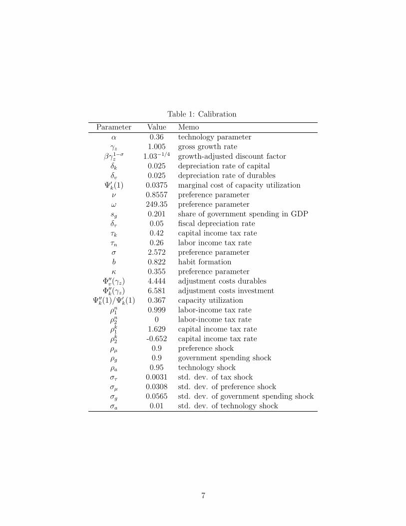
Table 1: Calibration

Parameter Value Memoα 0.36 technology parameterγz 1.005 gross growth rate

βγ1−σz 1.03−1/4 growth-adjusted discount factorδk 0.025 depreciation rate of capitalδv 0.025 depreciation rate of durables

Ψ′k(1) 0.0375 marginal cost of capacity utilizationν 0.8557 preference parameterω 249.35 preference parametersg 0.201 share of government spending in GDPδτ 0.05 fiscal depreciation rateτk 0.42 capital income tax rateτn 0.26 labor income tax rateσ 2.572 preference parameterb 0.822 habit formationκ 0.355 preference parameter

Φ′′v(γz) 4.444 adjustment costs durables

Φ′′k(γz) 6.581 adjustment costs investment

Ψ′′k(1)/Ψ′

k(1) 0.367 capacity utilizationρn

1 0.999 labor-income tax rateρn

2 0 labor-income tax rateρk

1 1.629 capital income tax rateρk

2 -0.652 capital income tax rateρµ 0.9 preference shockρg 0.9 government spending shockρa 0.95 technology shockστ 0.0031 std. dev. of tax shockσµ 0.0308 std. dev. of preference shockσg 0.0565 std. dev. of government spending shockσa 0.01 std. dev. of technology shock

7

3 A Model-Based Test of the Transmission-Mechanism

Hypothesis

We wish to evaluate the hypothesis that, assuming the correct identification of tax shocks,

the Blanchard-Perotti and Romer-Romer models identify different transmission mechanism

of tax shocks on output. Using the DSGE model of the previous section as the data generating

process, we estimate the transmission mechanisms associated with the Blanchard-Perotti and

Romer-Romer models. In so doing, we use our knowledge of the shocks driving the model

economy to leave completely aside the issue of identification.

3.1 Estimating the Blanchard-Perotti Transmission Mechanism

on Artificial Data

To estimate the Blanchard-Perotti reduced-form transmission mechanism, we draw a sample

of 1,000 quarters of the four disturbances of the model to produce time series for yt ≡ ln(yt/y),

τt ≡ ln(τt/τ), and gt ≡ ln(gt/g), denoting, respectively, the log-deviations from steady

state of detrended output, yt ≡ Yt/Zt, detrended tax revenues, τt ≡ Tt/Zt, and detrended

government spending, gt ≡ Gt/Zt. Tax revenues are given by Tt ≡ τnt Wtnt + τk

t (rtutKt −

δτKτt). The parameters y, τ , and g denote the steady-state values of yt, τt, and gt. We

keep only the last 250 observations of each artificial time series, which roughly corresponds

to the length of the postwar period, and discard the initial 750 observations. Our choice

of variables used for estimation is guided by the observation that in their empirical model

Blanchard and Perotti (2002) include output, tax revenues, and government spending.

The next step in our simulation exercise is to estimate the VAR system

Xt =

4∑

i=1

AiXt−i + ut,

8

where

Xt ≡

yt

τt

gt

.

Following Blanchard and Perotti (2002), we posit that the reduced form shock ut is related

to a vector of ‘fundamental’ shocks, εt, as

ut = Bεt,

where

εt ≡

ε1t

ε2t

ε3t

.

We note that because the DSGE model features four structural innovations and the size of

the VAR is three, the elements of εt cannot be interpreted as structural. Nevertheless, as

stated earlier, our exercise consists in taking for granted the identification of tax shocks and

examines instead the ability of the estimated VAR system to propagate that type of shock.

To this end, we identify ε1t with the tax shock and set the first column of the matrix B

equal to the impact effect of a unit increase in ετt on the vector Xt in the DSGE model. In

other words, the restriction we impose on the VAR system imply that the impulse responses

of output, tax revenues, and government spending implied by the DSGE and VAR models

are identical in the initial period. In subsequent periods, the true and estimated impulse

responses will in general be different.

We replicate this exercise 1,000 times and report the average impulse responses of tax

revenues and output to an innovation in ετt that raises tax revenues by one percent of steady-

state output on impact.

Figure 1 displays with blue solid lines the impulse responses of tax revenue and output

to a tax innovation implied by the DSGE model. The figure shows with red broken lines

9

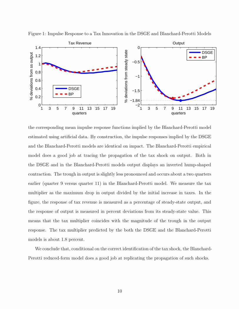
Figure 1: Impulse Response to a Tax Innovation in the DSGE and Blanchard-Perotti Models

1 3 5 7 9 11 13 15 17 190

0.2

0.4

0.6

0.8

1

1.2

1.4

quarters

% d

evia

tions

from

ss

outp

ut

Tax Revenue

DSGEBP

1 3 5 7 9 11 13 15 17 19−2

−1.84

−1.5

−1

−0.5

0

quarters

% d

evia

tions

from

ste

ady

stat

e

Output

DSGEBP

the corresponding mean impulse response functions implied by the Blanchard-Perotti model

estimated using artificial data. By construction, the impulse responses implied by the DSGE

and the Blanchard-Perotti models are identical on impact. The Blanchard-Perotti empirical

model does a good job at tracing the propagation of the tax shock on output. Both in

the DSGE and in the Blanchard-Perotti models output displays an inverted hump-shaped

contraction. The trough in output is slightly less pronounced and occurs about a two quarters

earlier (quarter 9 versus quarter 11) in the Blanchard-Perotti model. We measure the tax

multiplier as the maximum drop in output divided by the initial increase in taxes. In the

figure, the response of tax revenue is measured as a percentage of steady-state output, and

the response of output is measured in percent deviations from its steady-state value. This

means that the tax multiplier coincides with the magnitude of the trough in the output

response. The tax multiplier predicted by the both the DSGE and the Blanchard-Perotti

models is about 1.8 percent.

We conclude that, conditional on the correct identification of the tax shock, the Blanchard-

Perotti reduced-form model does a good job at replicating the propagation of such shocks.

10

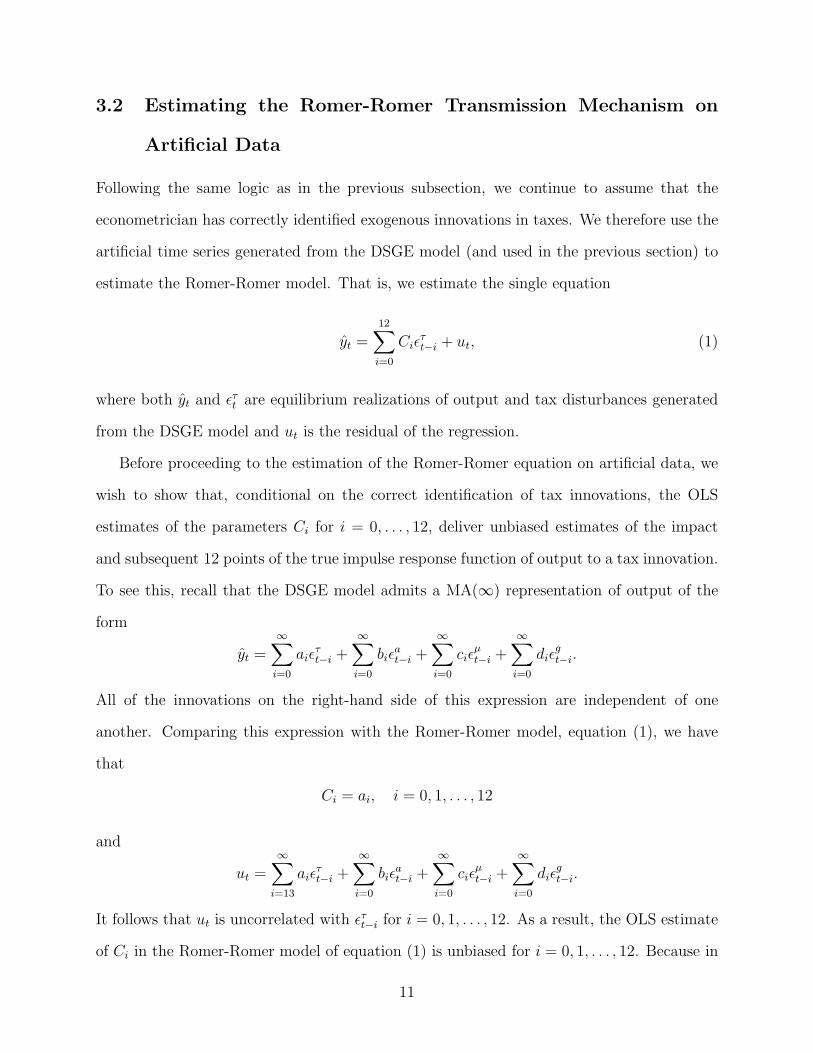
3.2 Estimating the Romer-Romer Transmission Mechanism on

Artificial Data

Following the same logic as in the previous subsection, we continue to assume that the

econometrician has correctly identified exogenous innovations in taxes. We therefore use the

artificial time series generated from the DSGE model (and used in the previous section) to

estimate the Romer-Romer model. That is, we estimate the single equation

yt =12∑

i=0

Ciετt−i + ut, (1)

where both yt and ετt are equilibrium realizations of output and tax disturbances generated

from the DSGE model and ut is the residual of the regression.

Before proceeding to the estimation of the Romer-Romer equation on artificial data, we

wish to show that, conditional on the correct identification of tax innovations, the OLS

estimates of the parameters Ci for i = 0, . . . , 12, deliver unbiased estimates of the impact

and subsequent 12 points of the true impulse response function of output to a tax innovation.

To see this, recall that the DSGE model admits a MA(∞) representation of output of the

form

yt =∞∑

i=0

aiετt−i +

∞∑

i=0

biεat−i +

∞∑

i=0

ciεµt−i +

∞∑

i=0

diεgt−i.

All of the innovations on the right-hand side of this expression are independent of one

another. Comparing this expression with the Romer-Romer model, equation (1), we have

that

Ci = ai, i = 0, 1, . . . , 12

and

ut =∞∑

i=13

aiετt−i +

∞∑

i=0

biεat−i +

∞∑

i=0

ciεµt−i +

∞∑

i=0

diεgt−i.

It follows that ut is uncorrelated with ετt−i for i = 0, 1, . . . , 12. As a result, the OLS estimate

of Ci in the Romer-Romer model of equation (1) is unbiased for i = 0, 1, . . . , 12. Because in

11

Figure 2: Impulse Response to a Tax Innovation in the DSGE and Romer-Romer Models

1 3 5 7 9 11 13 15 17 190

0.2

0.4

0.6

0.8

1

1.2

1.4

quarters

% d

evia

tions

from

ss

outp

ut

Tax Revenue

DSGERR

1 3 5 7 9 11 13 15 17 19−2

−1.84

−1.5

−1

−0.5

0

quarters

% d

evia

tions

from

ste

ady

stat

e

Output

DSGERR

our DSGE model the trough of the impulse response function of output to a tax innovation

occurs before period 12, it follows that the estimates of the Romer-Romer reduced-form

transmission mechanism of equation (1) deliver unbiased estimates of the tax multiplier.

The OLS estimate of Ci is, however, not efficient because the vector ut is serially correlated.

We explore this issue further in section 5.

Figure 2 displays the responses of tax revenues and output to an innovation in taxes

in the DSGE and Romer-Romer models. The Romer-Romer impulse responses correspond

to the average of 1,000 estimates of equation (1). The Romer-Romer reduced-form model

captures almost perfectly the true impulse response functions. In particular, it replicates the

true tax multiplier of 1.8 in period 11.

To preserve comparison with the Blanchard-Perotti model, we have estimated a version of

the Romer-Romer model in which the explained variable is the level of output. The original

Romer-Romer model, however, features the growth rate of output as the independent variable

in an equation of the form

∆yt =

12∑

i=0

Diετt−i + ut.

12

Figure 3: Impulse Response to a Tax Innovation in the DSGE and Difference-Romer-RomerModels

1 3 5 7 9 11 13 15 17 190

0.2

0.4

0.6

0.8

1

1.2

1.4

quarters

% d

evia

tions

from

ss

outp

ut

Tax Revenue

DSGERR−G

1 3 5 7 9 11 13 15 17 19−2

−1.84

−1.5

−1

−0.5

0

quarters%

dev

iatio

ns fr

om s

tead

y st

ate

Output

DSGERR−G

We note that our DSGE model implies that the growth rate of output possesses an MA(∞)

representation in the four structural shocks. Consequently, by the same argument given

in discussing the properties of the Romer-Romer model in levels, we have that an OLS

estimation of the Romer-Romer model in growth rates delivers unbiased estimates of the

coefficients Di for i = 0, 1, . . . , 12. As a corollary, the OLS estimator also delivers an unbiased

estimate of the tax multiplier at any horizon below 12 quarters.

Figure 3 displays the impulse responses of tax revenues and the level of output to a tax

innovation implied by the DSGE model and by the Romer-Romer model estimated using

output growth as the independent variable. The figure shows that the Romer-Romer model

in growth rates, like its counterpart in levels, captures nearly perfectly the transmission of

tax shocks to output. In particular, the Romer-Romer model estimated using the growth

rate of output uncovers the correct tax multiplier of 1.8 percent. For the remainder of the

paper, we focus on the Romer-Romer model featuring the level of output as the dependent

variable.

13

3.3 Evaluation of the Transmission-Mechanism Hypothesis

We have shown that, conditional on the correct identification of the exogenous tax distur-

bances, the average transmission mechanisms invoked by the Blanchard-Perotti and Romer-

Romer reduced-form models yield virtually identical tax multipliers, which, in turn, are in

line with the true multiplier associated with the DSGE data generating process. We take this

result as suggesting two alternative explanations for the fact that empirical estimates of the

Blanchard-Perotti and Romer-Romer models deliver significantly different tax multipliers.

One possible explanation is that actual estimated tax multipliers are different because of

small-sample undertainty. We explore this hypothesis in detail in section 5. A second possi-

ble explanation is that the Blanchard-Perotti and Romer-Romer regression models identify

fundamentally different tax disturbances.

4 Anticipation

We have established that conditional on the correct identification of tax innovations, both the

Blanchard-Perotti and Romer-Romer models satisfactorily capture the transmission mecha-

nism of tax disturbances. We now explore whether this continues to be the case when the

DSGE model is assumed to be driven by anticipated and unanticipated shocks. Schmitt-

Grohe and Uribe (2010a) argue that at least half of the variance of output and other macro-

economic aggregates are driven by anticipated shocks. Mertens and Ravn (2009) argue that

37 out of the 70 exogenous tax liability changes identified by Romer and Romer (2007)

are indeed anticipated, with a median anticipation horizon of six quarters. Anticipation

can potentially affect the ability of both the Blanchard-Perotti model and the Romer and

Romer model to capture the transmission mechanism of fiscal shocks. In the case of the

Blanchard-Perotti model, the VAR system is estimated using data driven by both antici-

pated and unanticipated shocks. In the case of the Romer-Romer model, the econometrician

regresses output onto a tax shock that is the sum of a purely unanticipated component and

14

a component that was announced in the past.

To introduce anticipation into the DSGE model, we assume the following specification

for the four structural disturbances:

εxt = νx0

t + νx6t−6,

for x = τ, µ, g, a. We assume that νx0t and νx6

t are distributed independently of each other and

across time with mean 0 and standard deviation σx0 and σx6, respectively. The innovation νx0t

is announced in period t and materializes in period t. That is, νx0t is a purely unanticipated

shock. The innovation νx6t is announced in period t and materializes in period t + 6. That

is, νx6t is a disturbance anticipated six quarters. We pick six quarters of anticipation for tax

shocks based on the finding of Mertens and Ravn (2009) referred to above. Schmitt-Grohe

and Uribe (2010b) present econometric evidence of anticipation in technology, government

spending, and preference shocks at horizons 4 and 8 quarters. For simplicity, we arbitrarily

assume anticipation horizons of six quarters for these three shocks.

The calibration of the model is as before. In particular, we assume that σ2a0 + σ2

a6 =

σ2a(= 0.012). We also assume that tax shocks, government spending shocks, and preference

shocks explain, respectively 20, 10, and 35 percent of the variance of output. Finally, we

assume that the variance of each shock is explained in equal parts by its anticipated and its

unanticipated components, that is, σ2x0 = σ2

x6 for x = τ, g, µ, a.

Figure 4 displays with solid lines the impulse responses to a surprise tax shock in the

DSGE model. Given that the model is approximated up to first order, these responses are

identical to those corresponding to the DSGE model featuring only unanticipated shocks.

The figure displays with broken lines the responses of the Blanchard-Perotti (top panels)

and Romer-Romer (bottom panels) models. As before, each model is estimated 1,000 times

on artificial data of length 250 quarter generated by the DSGE model, with 750 burn-in

periods.

15

Figure 4: Impulse Response to a Tax Innovation in the Blanchard-Perotti and Romer-RomerModels when the DSGE Model is Driven by Anticipated and Unanticipated Shocks

1 3 5 7 9 11 13 15 17 190

0.2

0.4

0.6

0.8

1

1.2

1.4

quarters

% d

evia

tions

from

ss

outp

ut

Tax Revenue

DSGEBP

1 3 5 7 9 11 13 15 17 19−2

−1.84

−1.5

−1

−0.5

0

quarters

% d

evia

tions

from

ste

ady

stat

e

Output

DSGEBP

1 3 5 7 9 11 13 15 17 190

0.2

0.4

0.6

0.8

1

1.2

1.4

quarters

% d

evia

tions

from

ss

outp

ut

Tax Revenue

DSGERR

1 3 5 7 9 11 13 15 17 19−2

−1.84

−1.5

−1

−0.5

0

quarters

% d

evia

tions

from

ste

ady

stat

e

Output

DSGERR

16

In the case of the Blanchard-Perotti model, we continue to assume that the econometri-

cian is able to identify the impact response of output and tax revenues to an unanticipated

tax shock. The coefficients of the VAR, however, are estimated using data from the DSGE

model driven by anticipated and unanticipated disturbances in taxes, preferences, technology,

and government spending. The figure shows that on average the Blanchard-Perotti model is

able to capture quite well the true impulse response functions. In particular, it delivers an

average tax multiplier of about 1.8, which is in line with its theoretical counterpart.

In the case of the Romer-Romer model, we run the following regression:

yt =12∑

i=0

Ci(ντ0t−i + ντ6

t−i−6) + ut.

Notice that ντ0t +ντ6

t−6 equals ετt , which is the total innovation in taxes materialized in period

t. This is the correct regression for the Romer-Romer model, because the econometrician is

not assumed to distinguish between anticipated and unanticipated tax disturbances. In spite

of the assumed inability of the econometrician to isolate the unanticipated tax innovation,

the regression recovers remarkably well the true impulse response to an unanticipated tax

shock. In particular, the estimated Romer-Romer model correctly predicts an average tax

multiplier of 1.8 percent.

We note that, unlike in the economy driven only by unanticipated shocks, in the economy

under study here, the Romer-Romer regression does not have a theoretical underpinning.

To see this, note that the MA(∞) representation of yt implied by the DSGE model with

anticipation is of the form

yt =∞∑

i=0

C0i ν

τ0t−i +

∞∑

i=0

C6i ντ6

t−i + rest,

where in this equation the term labeled ‘rest’ is orthogonal to the anticipated and unantici-

pated tax disturbances that appear on the right hand side.

By regressing yt onto ντ0t−i + ντ6

t−6−i, the Romer-Romer regression incorrectly imposes the

17

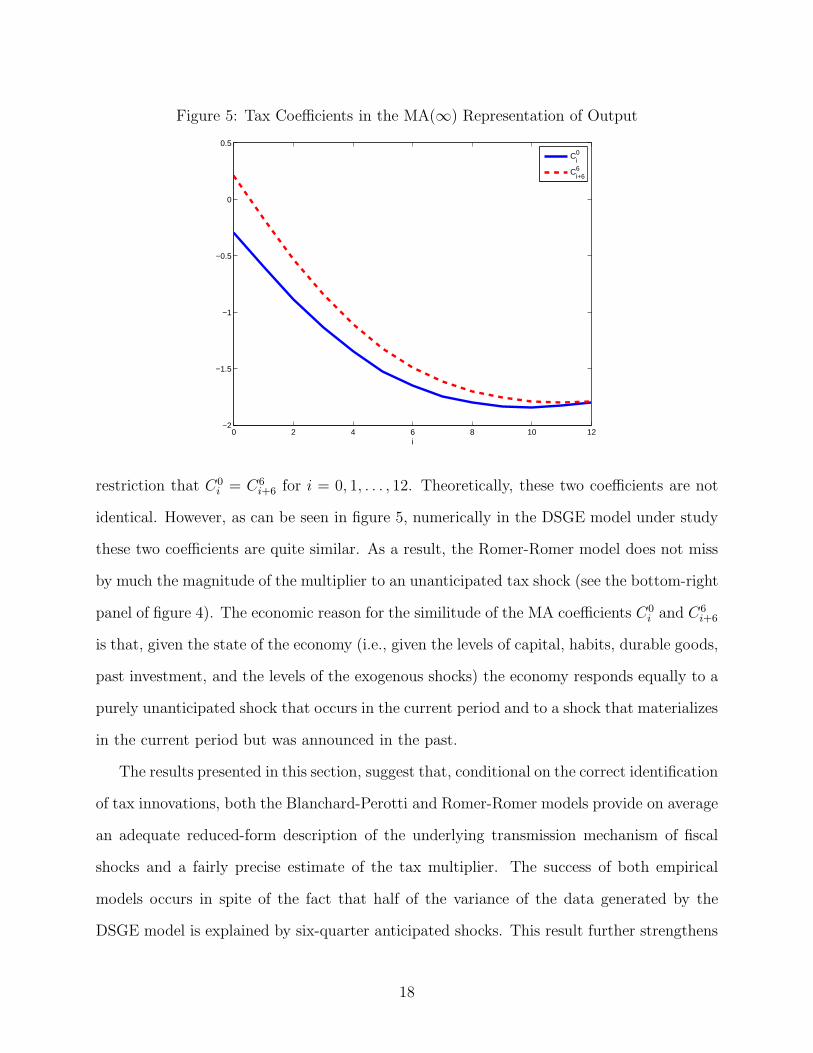
Figure 5: Tax Coefficients in the MA(∞) Representation of Output

0 2 4 6 8 10 12−2

−1.5

−1

−0.5

0

0.5

i

C0i

C6i+6

restriction that C0i = C6

i+6 for i = 0, 1, . . . , 12. Theoretically, these two coefficients are not

identical. However, as can be seen in figure 5, numerically in the DSGE model under study

these two coefficients are quite similar. As a result, the Romer-Romer model does not miss

by much the magnitude of the multiplier to an unanticipated tax shock (see the bottom-right

panel of figure 4). The economic reason for the similitude of the MA coefficients C0i and C6

i+6

is that, given the state of the economy (i.e., given the levels of capital, habits, durable goods,

past investment, and the levels of the exogenous shocks) the economy responds equally to a

purely unanticipated shock that occurs in the current period and to a shock that materializes

in the current period but was announced in the past.

The results presented in this section, suggest that, conditional on the correct identification

of tax innovations, both the Blanchard-Perotti and Romer-Romer models provide on average

an adequate reduced-form description of the underlying transmission mechanism of fiscal

shocks and a fairly precise estimate of the tax multiplier. The success of both empirical

models occurs in spite of the fact that half of the variance of the data generated by the

DSGE model is explained by six-quarter anticipated shocks. This result further strengthens

18

the main thesis of this paper, namely, that the differences in tax multipliers implied by

estimates of the Blanchard-Perotti and Romer-Romer models on actual data might be due

to factors other than the transmission mechanisms that these models invoke.

5 Small Sample Uncertainty and Tax Multipliers

Thus far we have concentrated attention on the average responses of the Blanchard-Perotti

and Romer-Romer models to tax shocks. These averages were taken over 1,000 samples of

artificial data, each 250 quarters long. As explained earlier, the sample size of 250 quarters is

meant to roughly capture the length of the postwar period. We now address the issue of small

sample uncertainty. This analysis will allow us to answer questions such as how likely it is to

observe within a finite sample of 250 quarters an estimate of the Romer-Romer tax multiplier

that exceeds the Blanchard-Perotti multiplier by two percentage points, conditional on the

correct identification of the tax shock. The difference of two percentage points reflects the

difference between the two multipliers when estimated on actual U.S. postwar data.

We characterize the distribution of tax multipliers at horizons 10, 11, and 12 quarters.

The tax multiplier at horizon 11, for instance, is defined as the percentage deviation of

output from steady state in period 11 triggered by an increase in tax revenues in period 1

equivalent to 1 percent of output. We focus on horizons 10, 11, and 12 quarters because in

our assumed data generating process the maximum contraction in output in response to an

exogenous unanticipated tax innovation occurs in quarter 11.

The top panel of table 2 displays summary statistics of tax multipliers obtained from 1000

samples of 250 quarters of artificial data generated using the DSGE model. As discussed

in previous sections, the mean of the tax multiplier implied by the Blanchard-Perotti and

Romer-Romer models is quite close to the true multiplier of 1.8. But, as the top panel of

the table shows, the short sample uncertainty surrounding both estimates is quite large,

as reflected in the standard deviation of the multiplier estimates over the 1,000 samples.

19

Table 2: Small Sample Properties of the Blanchard-Perotti and Romer-Romer Tax MultiplierConditional on the Correct Identification of Tax Shocks

Horizon mBP mRR Probability(qrt.) Mean Median Std.Dev. Mean Median Std.Dev. mRR > mBP mRR − mBP > 2

Sample Size 250 Quarters10 1.71 1.64 0.96 1.88 1.90 2.04 0.53 0.1711 1.69 1.62 0.97 1.90 1.94 2.04 0.54 0.1712 1.65 1.59 0.97 1.90 1.85 2.04 0.55 0.18

Sample Size 1000 Quarters10 1.80 1.79 0.47 1.82 1.74 0.95 0.48 0.0211 1.79 1.78 0.47 1.83 1.77 0.94 0.50 0.0112 1.77 1.75 0.47 1.83 1.75 0.94 0.50 0.02

Note: mBP and mRR stand for the tax multipliers implied by the Blanchard-Perotti and Romer-Romer models, respectively. All statistics are computed from 1000 samples of artificial datagenerated from the DSGE model.

The Romer-Romer multiplier estimate appears to be substantially more vulnerable to small-

sample uncertainty. Its associated standard deviation is twice as large as the one associated

with the Blanchard-Perotti estimate. This suggests that, conditional on the ability of both

models to correctly identify exogenous tax shocks, the Blanchard-Perotti model delivers a

more efficient estimate of the tax multiplier.

The penultimate column of table 2 shows that the estimated Romer-Romer tax multiplier

can be larger or smaller than the Blanchard-Perotti multiplier with almost equal probability.

The last column shows that the probability that in a sample of 250 quarters the Romer-

Romer multiplier is two percentage points larger than the Blanchard-Perotti multiplier (as

estimated in actual data) is 17 percent. This means that one cannot reject the hypothesis

that, conditional on correct identification, the observed differences in estimated tax multi-

pliers is due to small sample uncertainty.

The bottom panel of table 2 suggests that, conditional on the correct identification of

tax shocks, both the Blanchard-Perotti and Romer-Romer reduced-form models produce

consistent estimates of the tax multiplier. As the number of observations increases from 250

to 1000 quarters, the standard deviations of both estimates fall by half, and the probability

20

of observing a Romer-Romer multiplier that exceeds the Blanchard-Perotti multiplier by two

percentage points falls from 17 percent to 2 percent.

6 Hybrid Specifications

In a recent contribution, Favero and Giavazzi (2010) augment the Blanchard-Perotti model

by including the Romer-Romer shock as a regressor. They then compute the tax multiplier

induced by an innovation in the Romer-Romer shock. Favero and Giavazzi find that the size

of the multiplier is around unity, in line with the results of Blanchard and Perotti (2002).1

They argue that their combined model is the best approach to measure tax multipliers. The

key premise of their paper is that both the Blanchard-Perotti and the Romer-Romer models

correctly identify exogenous tax innovations. They interpret their findings, therefore, as

suggesting that the Romer-Romer single-equation model fails to capture the transmission of

tax shocks onto output.

We have shown that conditional on the correct identification of tax shocks, both the

Blanchard-Perotti and the Romer-Romer models produce the correct transmission mech-

anism and tax multipliers on average. We have also shown, again conditional on correct

identification, that the Blanchard-Perotti model yields more efficient estimates of the tax

multiplier than does the Romer-Romer model when small sample uncertainty is taken into

account. In light of these findings, we analyze the Favero-Giavazzi specification along two

dimensions, namely, bias and efficiency of the estimated tax multiplier.

We consider the following version of the Favero-Giavazzi model:

Xt =

4∑

i=1

AiXt−i + Cετt + ut,

1Mertens and Ravn (2009) also estimate a hybrid specification that combines a VAR system with theRomer-Romer tax shock as a regressor. In their specificaiton, these auhors distinguish between anticipatedand unanticipated Romer-Romer shocks. Unlike Favero and Giavazzi (2010), Mertens and Ravn estimate atax multiplier of around 2 percent. This difference deserves study.

21

Figure 6: Impulse Response to a Tax Innovation in the DSGE and Favero-Giavazzi Models

1 3 5 7 9 11 13 15 17 190

0.2

0.4

0.6

0.8

1

1.2

1.4

quarters

% d

evia

tions

from

ss

outp

ut

Tax Revenue

DSGEFG

1 3 5 7 9 11 13 15 17 19−2

−1.84

−1.5

−1

−0.5

0

quarters

% d

evia

tions

from

ste

ady

stat

e

Output

DSGEFG

where the notation is as in earlier sections. As in our previous Montecarlo exercises, we

estimate this version of the Favero-Giavazzi model 1,000 times. Each estimation uses a

sample of 250 quarters generated using the DSGE model. Figure 6 displays with solid lines

the response to a tax innovation implied by the DSGE model and with broken lines the

average response implied by the Favero-Giavazzi model. Like the Blanchard-Perotti and

Romer-Romer models, on average the Favero-Giavazzi model does a good job at uncovering

the transmission mechanism of tax innovations. We conclude that, conditional on the correct

identification of the tax shock, the Favero-Giavazzi model produces an unbiased estimate of

the tax multiplier. In this respect, therefore, the reduced-form transmission mechanisms

invoked by the Blanchard-Perotti, Romer-Romer, and Favero-Giavazzi models are on equal

footing.

But is the Favero-Giavazzi estimate of the tax multiplier more efficient than the one

produced by the Blanchard-Perotti or Romer-Romer models? We find that for a sample size

of 250 quarters, the estimate of the tax multiplier at a horizon of 11 quarters implied by

the Favero-Giavazzi model has a standard deviation across the 1,000 samples of 1.1. This

figure is slightly larger than the standard deviation of 0.97 found for the Blanchard-Perotti

estimate and significantly smaller than the standard deviation of the Romer-Romer estimate

22

(see table 2). We conclude that, conditional on the correct identification of the tax shock,

the Favero-Giavazzi model produces a more efficient estimate than the Romer-Romer model,

but offers no efficiency gains with respect to the Blanchard-Perotti model.

7 Conclusion

Since the revolutionary ideas of Keynes, governments have been fighting recessions with

spending increases and tax cuts. The justification of these policy measures often references

estimates offiscal multipliers. But the literature on the size of fiscal multipliers, be it tax

or government spending multipliers, does not speak with one voice. The VAR literature

delivers tax multipliers of about one percent, whereas the narrative literature produces tax

multipliers of about three percent. These differences are sizable enough to leave policymakers

without a clear guidance on the power of tax cuts to stimulate the economy.

The VAR and narrative approaches differ along two important dimensions. One is the

assumed transmission mechanism. The second is the methodology for identifying tax shocks.

This paper uses a micro-founded data-generating process to evaluate the hypothesis that

differences in estimated tax multipliers are due to differences in the assumed transmission

mechanism. In testing this hypothesis, it is assumed that both methodologies identify the

same tax shock. The main finding of this paper is that this hypothesis is rejected. Both

reduced-from models correctly uncover the size of the underlying tax multiplier.

Our results leave open two alternative explanations for the observed differences in es-

timated tax multipliers. One is small sample uncertainty. Accordingly, we explore the

small-sample properties of the estimated tax multipliers stemming from the VAR and nar-

rative models. We find that, conditional on both models identifying the same tax shock,

small sample uncertainty is large. In fact, small sample uncertainty accounts for all of the

observed differences in estimated tax multipliers according to our data generating process.

All of the results reported in this investigation are conditional on the assumption that

23

the VAR and narrative approaches successfully identify exogenous innovations in taxes. An

alternative explanation of the observed differences in estimates of tax multipliers is, of course,

that the two methodologies fail to identify the same tax shock. We believe that this alter-

native warrants future investigation.

24

References

Blanchard, Olivier and Roberto Perotti, “An Empirical Characterization of the Dynamic

Effects of Changes in Government Spending and Taxes on Output,” Quarterly Journal

of Economics 117, November 2002, 1329-1368.

Favero, Carlo, and Francesco Giavazzi, “VAR-BAsed and Narrative Measures of the Tax

Multiplier,” manuscript, Universita Bocconi, May 2010.

Mertens, Karel, and Morten O. Ravn, “Empirical Evidence on the Aggregate Effects of

Anticipated and Unanticipated U.S. Tax Policy Shocks,” Cornell University, 2009.

Romer, Christina, and David H. Romer, “The Macroeconomic Effects of Tax Changes:

Estimates Based on a New Measure of Fiscal Shocks,” NBER Working Paper No. 13264,

July 2007.

Schmitt-Grohe, Stephanie and Martın Uribe, “What’s News in Business Cycles,” Columbia

University, April 2010a.

Schmitt-Grohe, Stephanie and Martin Uribe, “Business Cycles With A Common Trend in

Neutral and Investment-Specific Productivity,” NBER Working Paper No. 16071, June

2010b.

25