A model for warehouse layoutKEES JAN ROODBERGEN1,∗ and IRIS F.A. VIS21 RSM Erasmus University, P.O. box 1738, 3000 DR Rotterdam, The Netherlands2 Vrije Universiteit Amsterdam, Faculty of Economics and Business Administration, De Boele-laan 1105, Room 3A-31, 1081 HV Amsterdam, The Netherlands

Please refer to this article as:Roodbergen, K.J. and Vis, I.F.A. (2006), A model for warehouse layout. IIE Transactions

38(10), 799-811.

AbstractThis paper describes an approach to determine a layout for the order picking area in warehouses,such that the average travel distance for the order pickers is minimized. We give analyticalformulas by which the average length of an order picking route can be calculated for two differentrouting policies. The optimal layout can be determined by using such formula as an objectivefunction in a non-linear programming model. The optimal number of aisles in an order pickingarea appears to depend strongly on the required storage space and the pick list size.

1 Introduction

Order picking is the process by which products are retrieved from storage to satisfy customerdemand. In its simplest form, an order arrives at the warehouse and an order picker is sentinto the picking area with the customer’s list to retrieve the requested items from storage.Much research has been done to find methods to retrieve products from storage as efficientlyas possible. The high efforts in this area are partly caused by the fact that order picking is anextremely expensive activity. Typically, the order picking contributes most to the operationalcosts of a warehouse (Tompkins et al., 2003). For the time required to pick an order, we canroughly distinguish three components: traveling between items, picking of items and remainingactivities. Picking the items consists of a series of actions ranging from positioning the vehicleto putting the picked items on a product carrier. The remaining activities include picking upan empty pick carrier, the acquisition of information, and dropping off the full pick carrier atsome point after picking is complete. Most efforts to improve the operational efficiency of orderpicking can be categorized into three groups of operating policies, namely routing, batching,and storage assignment. Each of these approaches generally focuses on reducing travel timessince these are easiest to influence. The time required for picking and remaining activities isinfluenced by aspects such as the chosen rack type and training of personnel.

Routing concerns the traveling of the order picker from location to location to retrieve prod-ucts. Usually, a large part of an order picker’s time is spent on traveling. Therefore this isan important aspect to consider. Research has focused on developing and comparing variousrouting methods. For example, Petersen (1997) gives a number of routing methods for ware-houses with a ladder-structure, i.e. a warehouse with a number of parallel aisles where orderpickers can change aisles in the front and rear cross aisle of the warehouse. Cross aisles are aislesperpendicular to the pick aisles and can be used to change from one aisle to the next. Rout-ing methods vary from simple heuristics to optimization schemes using dynamic programming.Two frequently used heuristics will be used in this paper and are explained below. A dynamic

∗Corresponding author

1

programming approach for routing in a warehouses with an added cross aisle in the middle isgiven in Roodbergen and De Koster (2001).

With batching several orders or partial orders are combined to create one or more pickingroutes. One form is to aggregate all available orders and to pick each product type individually.Another form is to combine several complete orders into one picking route. Numerous interme-diate forms exist. Much research is performed in this area, especially on methods that combinecomplete orders into a single route, see e.g. De Koster et al. (1999b) or Ruben and Jacobs(1999). If an order picker retrieves several orders at the same time, there are two possibilities:either the products are sorted by order while picking (sort-while-pick) or the order integrity isrestored after picking is completed (pick-and-sort). For sort-while-pick a special vehicle maybe required to separate the various orders. For pick-and-sort a manual or automated sortingsystem may be needed. A situation where multiple pickers work on the same order can be foundin areas with zoning, i.e. where each order picker only picks those products from an order thatare located in his assigned part of the warehouse.

Research concerning storage assignment focuses mainly on rules to assign products to loca-tions. Existing rules range from random, where new storage locations are assigned to productsrandomly, to full-turnover storage, where products with the highest pick frequency are assignedto the easiest accessible locations. Intermediate forms also exist, such as ABC-storage, wherethe A, B, and C categories are determined based on pick frequencies but storage within thecategories is random (see e.g. Petersen and Schmenner, 1999).

A common objective for order-picking systems is to maximize the service level subject toresource constraints such as labor, machines, and capital. The service level is composed of avariety of factors such as response time, order integrity, and accuracy. A crucial link betweenorder picking and service level is that the faster an order can be retrieved, the sooner it is availablefor shipping to the customer. If an order misses its shipping due time, it may have to wait untilthe next shipping period. Also, short order retrieval times imply high flexibility in handling latechanges in orders. Minimizing the order retrieval time (or picking time) is, therefore, a needfor any order-picking system. Possible improvements by changing the operating policies arerestricted by the physical layout of the area. That is, given a certain layout of the picking area,a good mix of operating policies can be chosen. In this paper, we will take the reverse approach.We propose a method that can find a layout that optimizes the order picking efficiency, givencertain operating policies. Such a method allows designers to take operational efficiency factorsinto account while designing the warehouse. Specifically, we formulate a non-linear programmingmodel to optimize the layout with respect to average travel distances.

In Section 2 we describe a model to find the best layout in a picking area consisting ofone block. In Section 3 estimates are developed for the average travel distance of two commonrouting policies. In Section 4 the location of the depot is discussed. In Section 5 the resultsfrom the travel distance estimates are compared with simulation and with existing estimatesfrom the literature. Section 6 describes some layout experiments. Layout differences resultingfrom the optimization with different routing policies are analyzed in Section 7. Conclusions aregiven in Section 8.

2 A model for layout optimization

We consider a manual order picking operation, where order pickers walk or drive through apicking area to retrieve products from storage. Picked items are placed on a vehicle, which theorder picker takes with him on his route. With some minor changes, we can also optimize otherpicking environments with this model, see Section 3.4. The picking area is rectangular with no

2

unused space and consists of a number of parallel aisles. At the front and rear of the pickingarea there is a cross aisle to enable aisle changes. An example of a layout of such a picking areais given in Fig. 1. Solid black squares in the figure indicate sections in the rack where itemshave to be picked.

Order pickers are assumed to be able to traverse an aisle in either direction and to changedirection within an aisle. Items are stored on both sides of the aisles. Item locations are deter-mined randomly according to a uniform distribution. We consider this storage assignment policybecause it can be considered as a base-line against which layouts with other storage assignmentpolicies can be compared. Furthermore, random storage is frequently used in practice. Thisoccurs, for example, in situations where the product assortment changes too fast to producereliable statistics about demand frequency (see e.g. De Koster et al., 1999a). Previous workon travel distance estimation for random storage is described in Hall (1993). Estimations in anactivity based storage environment are described in for example Caron et al. (1998) and Chewand Tang (1999). Each order consists of a number of items, which can and will be picked ina single route (such a "pick order" can be the result of a batching procedure, though). Pickedorders have to be deposited at the depot, where the picker also receives the instructions for thenext route. The depot is located in the front cross aisle.

We use two routing policies called the S-shape (or traversal) policy and the largest gap policy.These policies are widely used in practice (see Hall, 1993). With the S-shape policy, any aislecontaining at least one item is traversed through the entire length. Aisles where nothing has tobe picked are not entered. After picking the last item, the order picker returns to the front endof the aisle. With the largest gap policy, the picker enters the first aisle and traverses this aisleto the back of the warehouse. Each subsequent aisle is entered up to the ‘largest gap’ and leftfrom the same side as it was entered. A gap represents the distance between any two adjacentitems, or between a cross aisle and the nearest item. The last aisle is traversed entirely and thepicker returns to the depot along the front entering again each aisle up to the largest gap. Thus,the largest gap is the part of the aisle that is not traversed. Fig. 1 contains routes found byapplying the S-shape and largest gap policies to an example situation.

XXXXXXXXXXXXXXInsert figure 1XXXXXXXXXXXXXXTo find the layout that results in minimal average travel distances, we first have to find an

analytical expression that expresses the average travel distance as a function of a number oflayout arguments. We distinguish the following variables that influence average travel distance:

n the number of aisles (integer);

y the length of each of the aisles (real);

d the depot location, 1 ≤ d ≤ n (real).

The depot can be located anywhere in the front cross aisle between the left-most aisle (aisle 1)and the right-most aisle (aisle n). The position is indicated with a number. For example, d = 1indicates that the depot is located at the head of aisle 1; d = 3.5 indicates that the depot islocated between aisles 3 and 4.

Furthermore, we define the following parameters:

m the number of picks per route (integer);

3

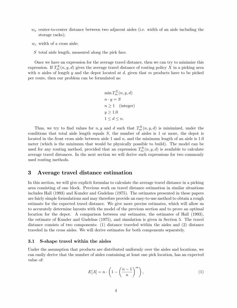
wa center-to-center distance between two adjacent aisles (i.e. width of an aisle including thestorage racks);

wc width of a cross aisle;

S total aisle length, measured along the pick face.

Once we have an expression for the average travel distance, then we can try to minimize thisexpression. If TX

m (n, y, d) gives the average travel distance of routing policy X in a picking areawith n aisles of length y and the depot located at d, given that m products have to be pickedper route, then our problem can be formulated as:

minTXm (n, y, d)

n · y = S

n ≥ 1 (integer)

y ≥ 1.01 ≤ d ≤ n.

Thus, we try to find values for n, y and d such that TXm (n, y, d) is minimized, under the

conditions that total aisle length equals S, the number of aisles is 1 or more, the depot islocated in the front cross aisle between aisle 1 and n, and the minimum length of an aisle is 1.0meter (which is the minimum that would be physically possible to build). The model can beused for any routing method, provided that an expression TX

m (n, y, d) is available to calculateaverage travel distances. In the next section we will derive such expressions for two commonlyused routing methods.

3 Average travel distance estimation

In this section, we will give explicit formulas to calculate the average travel distance in a pickingarea consisting of one block. Previous work on travel distance estimation in similar situationsincludes Hall (1993) and Kunder and Gudehus (1975). The estimates presented in these papersare fairly simple formulations and may therefore provide an easy-to-use method to obtain a roughestimate for the expected travel distance. We give more precise estimates, which will allow usto accurately determine layouts with the model of the previous section and to prove an optimallocation for the depot. A comparison between our estimates, the estimates of Hall (1993),the estimate of Kunder and Gudehus (1975), and simulation is given in Section 5. The traveldistance consists of two components: (1) distance traveled within the aisles and (2) distancetraveled in the cross aisles. We will derive estimates for both components separately.

3.1 S-shape travel within the aisles

Under the assumption that products are distributed uniformly over the aisles and locations, wecan easily derive that the number of aisles containing at least one pick location, has an expectedvalue of:

E[A] = n ·µ1−

µn− 1n

¶m¶, (1)

4

which is n times the probability that an aisle contains at least one pick. This is similar tothe formulations in Caron et al. (1998), Chew and Tang (1999), and Hall (1993). Actually thisis a good approximation of the expected number of aisles (see Kunder and Gudehus, 1975).

The expected value of the distance traveled inside the aisles for S-shape, DSy , can then be

stated as:

E[DSy ] = y0 ·E[A] + C (2)

where y0 = y+wc. That is, y0 is the length of an aisle plus two times the distance to go fromthe end of an aisle to the center of the cross aisle (two times 12wc). This distance is added sincewe assume that the order pickers walk through the middle of the cross aisles. C is a correctionterm that accounts for extra travel in the last aisle that is visited. This extra travel distanceoccurs if the number of aisles that has to be visited is an odd number. In this case the last aisleis both entered and exited from the front (see Fig. 1 for an example). In Hall (1993) and Kunderand Gudehus (1975) it is assumed that if the order picker has to turn in the last aisle, then thedistance traveled in this aisle is 2 · y0. That is, the last aisle first has to be traversed entirely tothe back of the warehouse before the order picker can return to the front. In manual pickingoperations, however, the order picker will generally return to the front directly after picking thelast item, instead of first going to the back of the warehouse. Caron et al. (1998) use a slightlydifferent routing policy. They assume that the order picker makes the turn in the aisle wherethe turn will be the shortest, instead of always turning in the last aisle. Furthermore, theyassume that the warehouse always has an even number of aisles. In practice, it will be difficultfor the order picker to know in which aisle to make the turn and the warehouse may have anodd number of aisles.

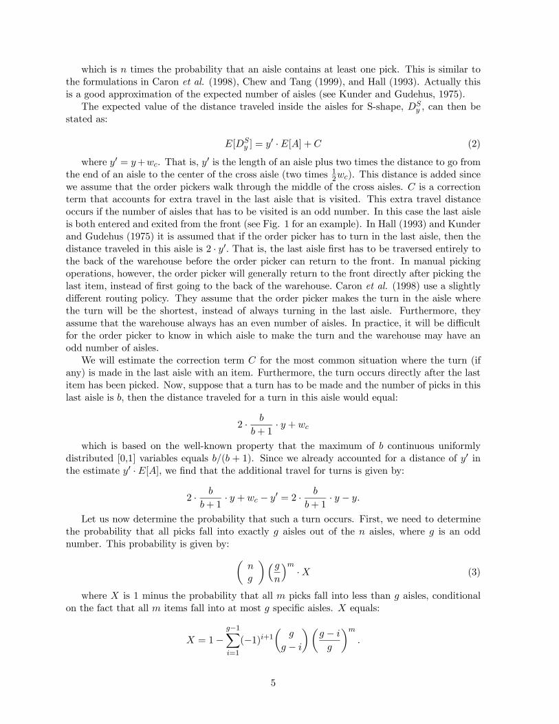
We will estimate the correction term C for the most common situation where the turn (ifany) is made in the last aisle with an item. Furthermore, the turn occurs directly after the lastitem has been picked. Now, suppose that a turn has to be made and the number of picks in thislast aisle is b, then the distance traveled for a turn in this aisle would equal:

2 · b

b+ 1· y + wc

which is based on the well-known property that the maximum of b continuous uniformlydistributed [0,1] variables equals b/(b + 1). Since we already accounted for a distance of y0 inthe estimate y0 ·E[A], we find that the additional travel for turns is given by:

2 · b

b+ 1· y + wc − y0 = 2 · b

b+ 1· y − y.

Let us now determine the probability that such a turn occurs. First, we need to determinethe probability that all picks fall into exactly g aisles out of the n aisles, where g is an oddnumber. This probability is given by: µ

ng

¶³ gn

´m ·X (3)

where X is 1 minus the probability that all m picks fall into less than g aisles, conditionalon the fact that all m items fall into at most g specific aisles. X equals:

X = 1−g−1Xi=1

(−1)i+1µ

g

g − i

¶µg − i

g

¶m

.

5

This result relies on the inclusion-exclusion rule. We start with a probability of 1 that allitems are in g aisles. We then subtract the probability that the items are in g − 1 or less aisles,which equals

¡ gg−1¢ ³g−1

g

´m. However, we have now subtracted the probability that all items

are in g − 2 or less aisles ¡ gg−1¢¡g−1

g−2¢times, but we should have only subtracted it

¡ gg−2¢times.

Therefore we have to add¡ gg−1¢¡g−1

g−2¢− ¡ g

g−2¢=¡ gg−2¢multiplied by

³g−2g

´m. However, now we

have added the probability that all items are in g − 3 aisles ¡ gg−3¢too often. And so on.

The correction term for the extra travel distance in the last aisle can be formulated as:

C =Xg∈G

"µng

¶³ gn

´m ·X ·Ã2 · y ·

mg

mg + 1

− y

!#where

G = {g | 1 ≤ g ≤ n, g ≤ m and g is odd} .

3.2 Largest gap travel within the aisles

In this section we will give an average travel distance estimate for another commonly used routingpolicy: largest gap. Based on results from Hall (1993) an estimate for the travel distance withinthe aisles with the largest gap policy can be obtained as:

n · y0 ·mXi=0

"µm

i

¶µ1

n

¶iµn− 1n

¶m−iDi

#(4)

where Di is a factor that denotes the expected travel distance on a line of length 1 if iitems are randomly distributed over this line. The values Di were obtained by simulation andtabulated in Hall (1993) for i = 1, ..., 10.

Formula 4 does not take into account that the first and last aisle are always entirely traversedwith largest gap routing. Furthermore, if all items are in one aisle, then the route should justconsist of entering and leaving that aisle from the front side. We will give a new estimate forlargest gap for which we distinguish between (1) the case where all items are in a single aisleand (2) the case where items are distributed over two or more aisles. For the second case weadd the additional time required to entirely traverse the first aisle and the last aisle with picks.

The probability that all items are in one aisle equals n · ¡ 1n¢m =¡1n

¢m−1and the average

distance traveled in that situation is simply 2y · mm+1 + wc. What remains to be estimated is

the distance traveled given that at least 2 aisles are to be visited. This event occurs with aprobability of 1 − ¡ 1n¢m−1 . Given that at least two aisles contain picks, we can estimate thenumber of aisles to visit by:

E[A | A ≥ 2] = E[A]− ¡ 1n¢m−11− ¡ 1n¢m−1

where E[A] is given by equation 1.To estimate the distance to be traveled in an aisle, we first obtain the probability:

P (i items in an aisle | i ≥ 1) = 1

1− ¡n−1n ¢mµmi¶µ

1

n

¶iµn− 1n

¶m−i.

6

Similar to Hall (1993) we can then multiply these probabilities by the related travel distanceto obtain an estimate for travel in the aisles if at least two aisles have to be visited:

1

1− ¡n−1n ¢m · (E[A | A ≥ 2]) ·mXi=1

µm

i

¶µ1

n

¶iµn− 1n

¶m−i(yDi +wcEi) (5)

where Di is identical to Hall (1993) and Ei (1 ≤ Ei ≤ 2) is a simulated estimate for the numberof times an aisles needs to be entered, given a certain number of picks in that aisle (the idea touse the estimate Ei is inspired by Ðukic and Oluic, 2001). The values for i = 1, ...50 are givenin Table 1.

Finally, we note that two of these aisles actually should be traversed entirely. We, therefore,subtract two aisles from equation 5 and add the distance of 2 full aisles, which is equal to2(y+wc), to the total estimate. This gives us as a total estimate for travel within the aisles withlargest gap routing:

E[DLGy ] =

µ1

n

¶m−1µ2y · m

m+ 1+wc

¶+

Ã1−

µ1

n

¶m−1!· 2(y + wc) +

1− ¡ 1n¢m−11− ¡n−1n ¢m · (E[A | A ≥ 2]− 2) ·

mXi=1

µm

i

¶µ1

n

¶iµn− 1n

¶m−i(yDi + wcEi) .

3.3 Travel within the cross aisles

The estimate for travel in the cross aisles is identical for S-shape and largest gap and consists ofthree components (1) travel from the depot to the left-most aisle with picks, (2) travel from aisleto aisle while picking items, and (3) travel from the right-most aisle with picks to the depot.See also Fig. 2 for a graphical illustration of the components.

XXXXXXXXXXXXXXInsert figure 2XXXXXXXXXXXXXXBoth Hall (1993) and Kunder and Gudehus (1975) assume that the depot is located in the

middle of the front cross aisle. Kunder and Gudehus (1975) determined the probability that allitems are distributed over a certain number, say f , aisles and estimated the distance traveled inthe cross aisles by 2·wa ·

³f−1f+1 · n− 1

´. That is, the distance in the cross aisles is estimated using

a property of f points distributed over a line according to a continuous uniform distribution.Hall (1993) uses the same property in a different way, estimating the distance in the cross aislesby 2 · wa · (n − 1) · m−1m+1 . Both approximations have the same two problems. First of all, adiscrete process is approximated using expected values for the continuous case. Secondly, it isassumed that for each route the depot is located between the left-most and right-most aisle withpicks. Situations in which all aisles with picks are on one side of the depot are neglected. As anexample of the possible impact of this deviation, consider a situation with d = 1 and m = 1. Inthis example, the actual expected travel distance in the cross aisles equals wa · (n − 1), whichis the distance from the depot to the middle of the warehouse and back. Both the formulationof Hall (1993) and Kunder and Gudehus (1975) will return an estimate of zero. This differencewill decrease if the number of picks m increases. Section 5 contains a comparison of the variousdistance estimates.

Firstly, we estimate the average distance from the depot to the right-most aisle containingitems. The probability that i is the right-most aisle to be visited is

¡in

¢m− ¡ i−1n ¢m which is the7

probability that all picks fall in aisles 1, ..., i minus the probability that all picks fall in aisles1, ..., i−1. The distance to be traveled is then the distance from depot location to the right-mostaisle. If aisle i would be the right-most aisle with items, then the distance to travel would bewa · |i− d|. Taking the sum over all values of i and multiplying by their probability of occurrencegives the expected distance to be traveled from the depot to the right-most aisle:

wa ·nXi=1

µ|i− d| ·

·µi

n

¶m

−µi− 1n

¶m¸¶. (6)

Similarly, we can find the distance from the depot to the left-most aisle to be:

wa ·nXi=1

µ|i− (n− d+ 1)| ·

·µi

n

¶m

−µi− 1n

¶m¸¶. (7)

Next we determine the estimate for the distance traveled in the cross aisles while pickingitems. We have n aisles numbered 1, ..., n from left to right. The estimated distance betweenthe left-most aisle containing picks and the right-most aisle containing picks is given by:

wa·nX<r

(r− )··µ

r − + 1

n

¶m

− 2µr −n

¶m

+

µr − − 1

n

¶m¸= wa·

Ã(n− 1)− 2 ·

n−1Xi=1

µi

n

¶m!

where the term between square brackets gives the probability that all m items fall in aisles, ..., r, at least one pick falls in and at least one pick falls in r.The expected value of the distance traveled in the cross aisles, Dx, can now be obtained by

adding all three components for cross aisle travel:

E[Dx] = wa ·Ãn− 1− 2 ·

n−1Xi=1

µi

n

¶m!

+wa ·nXi=1

µ(|i− d|+ |i− n+ d− 1|) ·

·µi

n

¶m

−µi− 1n

¶m¸¶.

3.4 Estimate for total average travel distance

Adding the two components (distance traveled in aisles and in cross aisles) gives the totalexpected travel distance in the picking area:

TXm (n, y, d) = E[DX

y ] +E[Dx].

This formulation has been developed for a manual picking operation. Therefore, we wereable to use the average travel distance as a performance criterion. If we analyzed, for example,an automated storage / retrieval system, then a better performance criterion would be averagetravel time, because travel speed in aisles and cross aisles is unequal in such an environment. Ifwe define ty as the travel speed in the aisles and tx as the travel speed in the cross aisles thenthe estimate for average travel time would be ty · E[Dy] + tx · E[Dx]. Furthermore, additionaltime may be required for each change of aisles to position the vehicle correctly, especially inan environment with a relatively large vehicle in narrow aisles. Since this extra time has to beadded each time the vehicle enters an aisle, we can just add tc ·E[A] to the travel time estimate

8

of S-shape, where tc is the time needed to enter an aisle. For largest gap we can easily build anappropriate expression using values of Ei from Table 1.

In practical situations it will often be the case that the pick list size is variable. The formulaswe developed are valid only for a fixed pick list size. However, they can easily be adapted forvariable pick list sizes. For example, assume that we know for every pick list size m thatit will occur with probability pm, then the estimate for average travel distance is given byP∞

m=1 pm · TXm (n, y, d).

Clearly, due to the nature of the approach we used (e.g. we assume that expected traveldistance in aisles and expected travel distance in cross aisles are independent), these formulationsgive approximations of actual average travel distances. We will test the performances of theformulas in Section 5.

4 Optimization of the depot location

Bassan et al. (1980) show that under the condition of random storage, the depot should belocated in the middle of the front cross aisle to minimize average travel distance. Their proofwas given in the context of a single command environment (i.e. each pick list contains only oneitem). We will show that it holds for any pick list size. Intuitively, a depot in the middle ofthe front cross aisle seems to be the best with respect to average travel time. In this way, theprobability seems to be highest that the depot is located between the left-most and right-mostaisle of a picking route, thus preventing extra travel time to go forth and back to this regionfrom a depot that is out of the middle. However, in the literature, as well as in practice, depotlocations vary. A depot located in the middle is used in Goetschalckx and Ratliff (1988), Hall(1993), Kunder and Gudehus (1975) and Petersen (1999). A depot located in a corner is usedin Chew and Tang (1999), De Koster et al. (1999b), Gibson and Sharp (1992), and Rosenwein(1996). Both middle and corner options are considered in Jarvis and McDowell (1991), Petersen(1997) and Petersen and Schmenner (1999).

TheoremThe depot location that minimizes average travel distance is the exact middle of the front crossaisle.

ProofThe depot location only influences average travel distance through the term (see equations 6and 7):

wa ·nXi=1

µ(|i− d|+ |i− n+ d− 1|) ·

·µi

n

¶m

−µi− 1n

¶m¸¶.

We distinguish 4 cases.Case 1: if i ≥ d and i+d ≥ n+1 then |i− d|+ |i− n+ d− 1| = i−d+ i−n+d−1 = 2i−n−1.Since 2i−n− 1 is independent of d there is no influence of the depot location on average traveldistance.Case 2: if i ≤ d and i+d ≥ n+1 then |i− d|+ |i− n+ d− 1| = d−i+i−n+d−1 = 2d−n−1.Travel distance is minimized by choosing d as small as possible under the condition that i ≤ dand i + d ≥ n + 1. Substituting i by d gives 2d ≥ n + 1 or d ≥ n+1

2 . This implies that traveldistance is minimized if d = n+1

2 , i.e. the depot is located in the middle of the front cross aisle.Case 3: if i ≥ d and i+d ≤ n+1 then |i− d|+|i− n+ d− 1| = i−d−i+n−d+1 = −2d+n+1.Travel distance is minimized by choosing d as large as possible under the condition that i ≥ d

9

and i + d ≤ n + 1. Substituting i by d gives 2d ≤ n + 1 or d ≤ n+12 . This implies that travel

distance is minimized if d = n+12 , i.e. the depot is located in the middle of the front cross aisle.

Case 4: if i ≤ d and i+d ≤ n+1 then |i− d|+|i− (n− d+ 1)| = d−i−i+n−d+1 = −2i+n+1.This is independent of the depot location.Thus, average travel distance is minimized by taking d = n+1

2 . ¥We have proven that the depot is to be located in the middle of the front cross aisle under

the conditions that random storage is used and that the depot location is restricted to the frontcross aisle. The proof holds for both S-shape routing and largest gap routing, since both havethe same amount of travel in the cross aisles. The above proof holds also for some other routingheuristics (for a description of other routing heuristics see e.g. Petersen, 1997) because theyhave exactly the same amount of cross aisle travel per route. An evaluation of the percentagedifference in average travel distance between a picking area with a depot located at the left anda picking area with a depot located in middle is included in the next section.

5 Model accuracy experiments

We compare the values calculated with the formulas from Section 3 with the results from sim-ulation. Furthermore, we will include the estimates of Hall (1993) and Kunder and Gudehus(1975) into our comparisons. For this comparison, we consider a manual picking operation in ashelf area, where several order pickers may be assigned to the same zone. The center-to-centerdistance between two neighboring aisles is 2.5 meters. Order pickers are assumed to travelthrough the exact middle of the aisles and cross aisles. Cross aisles are 2.5 meters wide. For thistype of picking areas we assume the following measures to be representative. Aisle length variesbetween 10 and 30 meters. Each order picker works in a zone consisting of 7 to 15 aisles. Weuse the extremes of these values for our comparison, which gives four different layouts. For eachlayout we consider three different values for the number of picks per route, namely 1, 10 and 30.Furthermore, for each situation we consider two depot locations: at the left (at the head of aisle1) and in the middle of the front cross aisle. For the simulation we generated 2000 orders for eachsituation. This number of replications is sufficient to obtain a 95% confidence interval with ahalf-width of less than 2% of the sample mean. Pick locations are distributed over the aisles andlocations according to a uniform distribution. No picks occur in the cross aisles. Tables 2 and 3give the results from the simulation, our formulas, and the existing formula(s) for respectivelyS-shape routing and largest gap routing. The percentage difference in Tables 2 and 3 betweensimulated and calculated values has been calculated before rounding of the route lengths.

From the results, we can see that the formulas of Hall (1993) and Kunder and Gudehus (1975)become less accurate if the number of picks decreases; deviations of more than 50% occur. Theresults from our formulas follow the behavior of the simulation closely. For each situation, theresults of our formulas are close to the simulation results. Therefore, average route length can bedetermined by straightforward calculations with our formulas instead of developing a simulationmodel for the order picking area. The quality of the estimates is especially important since wewish to use it to determine a layout. Errors in the distance estimates may result in an erroneousranking of the alternatives and, therefore, lead to the choice of a layout that is not as efficientas possible.

XXXXXXXXXXXXXXInsert tables 2 and 3XXXXXXXXXXXXXX

10

6 Some layout considerations for S-shape

We can use the model of Section 2 to determine the best layout for various values of the totalaisle length. Using formula 2, we determine average route length for 1, 2, 3, ... aisles whiledecreasing aisle length such that total aisle length is kept constant. The depot can be locatedin the middle of the front cross aisle, because we already showed in the previous section thatthe middle is the best location. Aisle length is determined by dividing total aisle length by thenumber of aisles and adding twice the distance needed to go from the end of the aisle to themiddle of the cross aisle (y0 = S/n+wc). By taking the number of aisles that give the minimumaverage route length, we obtain the best layout with respect to travel distance. Essentially, thismeans we suggest solving the layout model by complete enumeration. Even though enumerationis generally not the obvious approach, there is no strong need to search for a more efficientsolution method here. The solution space is very small, because the minimum aisle length is 1meter, and because the number of aisles is an integer value. Thus, for example, for a warehouselayout problem with S = 150, there are only 150 possible solutions, ranging from a layout with1 aisle of 150 meters to a layout with 150 aisles of 1 meter each. Calculation time for these 150possible layouts is less than 1 second on a 1.5 GHz personal computer.

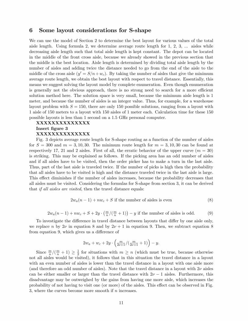
XXXXXXXXXXXXXXInsert figure 3XXXXXXXXXXXXXXFig. 3 depicts average route length for S-shape routing as a function of the number of aisles

for S = 300 and m = 3, 10, 30. The minimum route length for m = 3, 10, 30 can be found atrespectively 17, 21 and 2 aisles. First of all, the erratic behavior of the upper curve (m = 30)is striking. This may be explained as follows. If the picking area has an odd number of aislesand if all aisles have to be visited, then the order picker has to make a turn in the last aisle.Thus, part of the last aisle is traveled twice. If the number of picks is high then the probabilitythat all aisles have to be visited is high and the distance traveled twice in the last aisle is large.This effect diminishes if the number of aisles increases, because the probability decreases thatall aisles must be visited. Considering the formulas for S-shape from section 3, it can be derivedthat if all aisles are visited, then the travel distance equals:

2wa(n− 1) + nwc + S if the number of aisles is even (8)

2wa(n− 1) + nwc + S + 2y · ¡mn /(mn + 1)¢− y if the number of aisles is odd. (9)

To investigate the difference in travel distance between layouts that differ by one aisle only,we replace n by 2ν in equation 8 and by 2ν + 1 in equation 9. Then, we subtract equation 8from equation 9, which gives us a difference of

2wa + wc + 2y ·³

m2ν+1/(

m2ν+1 + 1)

´− y.

Since mn /(

mn + 1) ≥ 1

2 for situations with m ≥ n (which must be true, because otherwisenot all aisles would be visited), it follows that in this situation the travel distance in a layoutwith an even number of aisles is lower than the travel distance in a layout with one aisle more(and therefore an odd number of aisles). Note that the travel distance in a layout with 2ν aislescan be either smaller or larger than the travel distance with 2ν − 1 aisles. Furthermore, thisdisadvantage may be outweighed by the gains from having one more aisle, which increases theprobability of not having to visit one (or more) of the aisles. This effect can be observed in Fig.3, where the curves become more smooth if n increases.

11

From Fig. 3 we can also see that two aisles was the best option for the situation with a picklist size of n = 30. It would be interesting to know whether a higher pick density in generaltends to favor layouts with just 2 aisles. We evaluate the behavior of TS

m(n, y, d) if m approachesinfinity.

It is fairly straightforward to show that

limm→∞E[A] = n

limm→∞C =

½y if n is odd0 if n is even

limm→∞E[Dx] = wa(n− 1).

Because the probability that all aisles are visited approaches 1 if m→∞ it holds that thereis a shorter layout with an even number of aisles for each layout with an odd number of aisles.We, therefore, can restrict our search for a minimum to the situations for which n is even. Thus,

limm→∞TS

m(n, y, d) = limm→∞E[Dy] + lim

m→∞E[Dx]

= limm→∞((y + wc) ·E[A]) + lim

m→∞C + limm→∞E[Dx]

= (y + wc)n+ wa(n− 1) if n is even.

The minimum is obtained at n = 2 (there are no smaller even values). From a practical pointof view, it may be noted that a single picking area consisting of two aisles may not always beconvenient. Firstly, the shape may be difficult to fit into the overall warehouse design. Secondly,there is a risk of congestion, since all pickers would then be working in the same two aisles. Thiscould result in a zone-based approach for order picking, where each order picker is responsiblefor picking in two aisles. Obviously, this may require system changes, such as the inclusion of asorting area or the introduction of a method where picked items are passed from one picker tothe next ("pick-and-pass"). These changes would have to weighted against the benefits of traveltime reductions.

Finally, it is interesting to note from a practical point of view that curves appear to be quiteflat around the optimum (at least if the optimum is not equal to 2 aisles). That is, around theoptimum there are a large number of other layouts that have average travel distances whichare only a few percent higher. A designer may be able to use this flexibility to meet otherrequirements. Such requirements may include prevention of congestion, flexibility for redesignor stability with respect to changes in the pick list size. Instead of finding "the best" layout, adesigner may use the model to determine the k-best layouts and then choose from these layoutsbased on other considerations than travel time alone.

7 Influence of the routing policy on the layout

We have formulated a model to determine optimal layouts for a given routing policy. Further-more, we have derived two expressions for average travel distance, which can be used as objectivefunctions in the model. One objective function consists of a travel distance estimate for S-shaperouting and the other for largest gap routing. Given a certain choice for a specific routingmethod, it is now fairly straightforward to determine the best layout based on expected picklist size and the required storage space. In design practice, however, the layout is often chosen

12

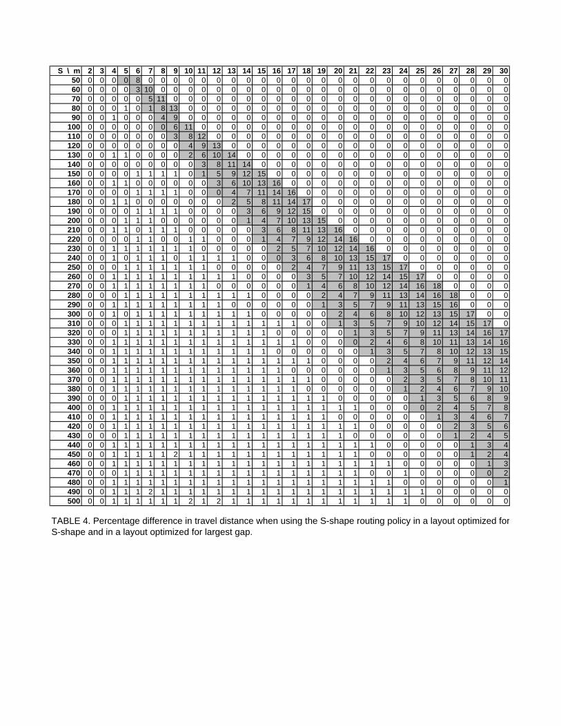
before the routing policy. It would, therefore, be interesting to know what the actual influenceof the routing policy is on the layout. Or, formulated differently, what is the loss in efficiencyif the layout is optimized with another routing policy than the policy that is actually going tobe used? We investigate this issue as follows. We take the same manual picking operation ina shelf area (i.e. wa = 2.5 and wc = 2.5) and determine the optimal layout for both routingpolicies for a range of sizes (S = 50, 60, 70, ..., 500) and pick list sizes (m = 2, 3, 4, ..., 30). Wethen calculate the expected travel distance when S-shape is used in the layout that has beenoptimized for S-shape and we calculate the expected travel distance when using S-shape in thelayout optimized for largest gap. The percentage difference between these two travel distancesis given in Table 4. A table for largest gap routing would be very similar.

XXXXXXXXXXXXXXInsert table 4XXXXXXXXXXXXXXAs can be seen from Table 4, there is only a small difference in travel distances for most

situations. The upper-right corner of the table contains only zeros because the optimal layout inthese situations consists of exactly 2 aisles regardless of the routing policy. The lower-left cornercontains situations where the optimal layout consists of strictly more than 2 aisles for bothrouting methods (though the exact number may differ). The grey area consists of situationswhere the optimal layout for S-shape consists of exactly 2 aisles and the optimal layout forlargest gap consists of strictly more than 2 aisles. As can be seen from the table, the onlysignificant differences occur in the last situation.

From the above experiment it can be seen that in many practical situations (namely thosewhere the majority of pick list sizes fall outside the grey area) there is no significant efficiencyloss if another routing method is used for the optimization than for the actual operation. Onthe other hand, large deviations (in our experiment up to 18%) may occur depending on therequired storage space and the pick list sizes. If the routing policy is undecided when the layouthas to be chosen, it may therefore be advisable to perform a sensitivity analysis on the variousrouting policies.

Another interesting point to consider is whether conditions can be identified when S-shapeor largest gap is to be preferred as a routing policy. From Hall (1993), it is known that S-shape ispreferred over largest gap if the number of picks per aisle exceeds 4. This rule, however, assumesthat the layout is already determined in advance. Using our model, we can compare routingpolicies together with their optimal layout. To illustrate the possibilities, we analyze an initialdesign for a shelf area (wa = 2.5; wc = 2.5) with 18 picks per route and 4 aisles of 75 meters each.Travel distance is then 324.4 meters for S-shape and 340.3 meters for largest gap. The optimallayout, however, consists of 23 aisles for S-shape and 20 aisles for largest gap. The resultingtravel distances are then 300.3 meters for S-shape and 246.6 meters for largest gap. Largest gapthus outperforms S-shape here. We have completed this experiment for S = 50, 60, 70, ..., 500and m = 2, 3, 4, ..., 30. For all these 1334 situations the largest gap policy gave travel distancesthat are equal to or shorter than the distances for the S-shape policy. The best layout - whenoptimized for largest gap - is for all situations such that the number of aisles equals 2 (i.e. largestgap and S-shape routing are the same) or the number of aisles is such that there are less than4 items per aisle. We repeated this experiment for pallet racks (wa = wc = 4) with the sameresults. It seems, therefore, that if layout still needs to be determined, then largest gap routingis generally to be preferred over S-shape routing.

13

8 Concluding remarks

In this paper we have evaluated the relation between the layout of the order picking area andthe average length of a picking route for areas consisting of one block. Analytical formulasare presented by which the average route length can be calculated for two different routingpolicies. The outcomes of the formulas depend on the number of aisles, the aisle length, thedepot location, the number of picks per route and some physical parameters of the racks. Theresults from the formulas are compared with simulation results. It appeared that the differencebetween simulated and calculated values was minor in all of our experiments. Therefore, weconsider the analytical formulas to be accurate enough to be used instead of simulation.

The analytical formulas can be used as objective function in the presented non-linear pro-gramming model to find an optimal layout for the order picking area in warehouses. We provedthat the best depot location is in the middle of the front cross aisle. The proof is valid forseveral routing heuristics under the condition that random storage is used. Given that S-shapewill be used for routing, we derived some general characteristics of "good" layouts. For highpicking densities, S-shape routing is best employed in a layout with an even number of aislesinstead of an odd number of aisles. From the viewpoint of strict travel distance minimization,a very high pick density is best dealt with in a picking area where each picking zone consists ofexactly two aisles. For practical implementations, other considerations than travel distance canbe taken into account easily too, since there are generally several layouts that have an averagetravel distance that is close to the optimum.

In a comparison of more than 2500 different layout problems, we found that largest gaprouting performed better than or equal to S-shape routing in all situations if the optimal layoutwas used for each routing method. The optimal layout is sensitive to the routing policy used inthe optimization. We found efficiency losses of up to 18% when optimizing the layout for anotherrouting policy than was used for the actual operation. It must also be noted that there are largeregions where the resulting travel distance is highly insensitive to the routing method used inthe optimization. Given these uncertain effects, it is advisable to perform the optimization formore than one routing method before deciding on the layout.

References

Bassan, Y., Roll, Y. and Rosenblatt, M.J. (1980) Internal layout design of a warehouse. AIIETransactions, 12(4), 317-322.

Caron, F., Marchet, G. and Perego, A. (1998) Routing policies and COI-based storage policiesin picker-to-part systems. International Journal of Production Research, 36(3), 713- 732.

Chew, E.P. and Tang, L.C. (1999) Travel time analysis for general item location assignmentin a rectangular warehouse. European Journal of Operational Research, 112(3), 582-597.

De Koster, R., Roodbergen, K.J. and Van Voorden, R. (1999a) Reduction of walking timein the distribution center of De Bijenkorf, in New Trends in Distribution Logistics, Speranza,M.G. and Stähly, P. (eds.), Springer, Berlin, pp. 215-234.

De Koster, M.B.M., Van der Poort, E.S. and Wolters, M. (1999b) Efficient orderbatchingmethods in warehouses. International Journal of Production Research, 37(7), 1479-1504.

Ðukic, G., and Oluic, C. (2001) Travel time models for order-picking, in Proceedings of the17th International Conference on CAD/CAM, Robotics and Factories of the Future, Janssens,W. (ed.), pp. 1087-1094.

Gibson, D.R. and Sharp, G.P. (1992) Order batching procedures. European Journal ofOperational Research, 58(1), 57-67.

14

Goetschalckx, M. and Ratliff, H.D. (1988) Order picking in an aisle. IIE Transactions, 20(1),53-62.

Hall, R.W. (1993) Distance approximations for routing manual pickers in a warehouse. IIETransactions, 25(4), 76-87.

Jarvis, J.M. and McDowell, E.D. (1991) Optimal product layout in an order picking ware-house. IIE Transactions, 23(1), 93-102.

Kunder, R. and Gudehus, T. (1975) Mittlere Wegzeiten beim eindimensionalen Kommission-ieren. Zeitschrift für Operations Research, 19, B53-B72 (in german).

Petersen, C.G. (1997) An evaluation of order picking routing policies. International Journalof Operations & Production Management, 17(11), 1098-1111.

Petersen, C.G. (1999) The impact of routing and storage policies on warehouse efficiency.International Journal of Operations & Production Management, 19(10), 1053-1064.

Petersen, C.G. and Schmenner, R.W. (1999) An evaluation of routing and volume-basedstorage policies in an order picking operation. Decision Sciences, 30(2), 481-501.

Roodbergen, K.J. and De Koster, R. (2001) Routing order pickers in a warehouse with amiddle aisle. European Journal of Operational Research, 133(1), 32-43.

Rosenwein, M.B. (1996) A comparison of heuristics for the problem of batching orders forwarehouse selection. International Journal of Production Research, 34(3), 657-664.

Ruben, R.A. and Jacobs, F.R. (1999) Batch construction heuristics and storage assignmentstrategies for walk/ride and pick systems. Management Science, 45(4), 575-596.

Tompkins, J.A., White, J.A., Bozer, Y.A. and Tanchoco, J.M.A. (2003) Facilities Planning,Wiley, New York, NY.

9 Captions

Fig. 1. Example of an order picking area, including example routes as found by the S-shapeheuristic (upper image) and the largest gap heuristic (lower image).

Fig. 2. Illustration of the three components for travel in the cross aisles.Fig. 3. Average route length in meters as a function of the number of aisles for three

different pick list sizes (indicated next to the curves). Total aisle length (S) equals 300 meters.Asterisks indicate the minimum for m = 3 and m = 10.

Table 1. Values of Di and Ei for i = 1, . . . , 50 (based on 1,000,000 replications).Table 2. Average route length in meters for picking an order with the S-shape routing

policy. For each of the formulas the percentage difference with the distance obtained from thesimulation is also given.

Table 3. Average route length in meters for picking an order with the largest gap routingpolicy. For each of the formulas the percentage difference with the distance obtained from thesimulation is also given.

Table 4. Percentage difference in travel distance when using the S-shape routing policy ina layout optimized for S-shape and in a layout optimized for largest gap.

10 Biographical sketches

Kees Jan Roodbergen is an Assistant Professor of Logistics and Operations Management atRSM Erasmus University, The Netherlands. He received his M.Sc. in Econometrics from theUniversity of Groningen, The Netherlands and his Ph.D. from the Erasmus University Rotter-

15

dam. His research interests include design and optimization of warehousing and cross dockingenvironments.

Iris F.A. Vis is an Associate Professor of Logistics at the Vrije Universiteit Amsterdam,The Netherlands. She holds an M.Sc. in Mathematics from the University of Leiden, TheNetherlands and a Ph.D. from the Erasmus University Rotterdam. She received the INFORMSTransportation Science Section Dissertation Award 2002. Her research interests are in designand optimization of container terminals, vehicle routing, and supply chain management.

16

i D i E i i D i E i1 0.500 1.000 26 1.712 1.9262 0.778 1.333 27 1.719 1.9293 0.958 1.500 28 1.727 1.9314 1.087 1.600 29 1.734 1.9335 1.183 1.667 30 1.740 1.9366 1.259 1.715 31 1.746 1.9377 1.321 1.750 32 1.752 1.9398 1.371 1.778 33 1.758 1.9419 1.414 1.800 34 1.763 1.943

10 1.451 1.818 35 1.768 1.94411 1.483 1.833 36 1.773 1.94612 1.511 1.846 37 1.777 1.94713 1.535 1.857 38 1.782 1.94914 1.558 1.867 39 1.786 1.95015 1.577 1.875 40 1.790 1.95116 1.595 1.883 41 1.794 1.95217 1.612 1.889 42 1.798 1.95418 1.627 1.895 43 1.801 1.95519 1.640 1.900 44 1.805 1.95620 1.653 1.905 45 1.808 1.95621 1.665 1.909 46 1.811 1.95722 1.675 1.913 47 1.814 1.95823 1.685 1.917 48 1.817 1.95924 1.695 1.920 49 1.820 1.96025 1.703 1.923 50 1.823 1.961

TABLE 1. Values of D i and E i for i = 1,…, 50 (based on 1,000,000 replications).

aisle number number depotlength of aisles of items location distance difference distance difference distance difference

10 7 1 left 27.0 15.0 -44.3% 18.8 -30.4% 27.5 2.0%10 7 1 middle 20.9 15.0 -28.3% 18.8 -10.3% 21.1 0.8%10 7 10 left 98.5 86.1 -12.6% 103.7 5.3% 99.0 0.5%10 7 10 middle 97.4 86.1 -11.6% 103.7 6.5% 97.7 0.4%10 7 30 left 121.8 100.8 -17.2% 125.6 3.2% 122.4 0.5%10 7 30 middle 121.7 100.8 -17.2% 125.6 3.2% 122.3 0.5%10 15 1 left 46.3 15.0 -67.6% 18.8 -59.5% 47.5 2.5%10 15 1 middle 30.9 15.0 -51.5% 18.8 -39.4% 31.2 0.7%10 15 10 left 159.1 127.9 -19.6% 161.1 1.2% 159.6 0.3%10 15 10 middle 154.4 127.9 -17.2% 161.1 4.3% 155.0 0.4%10 15 30 left 235.2 211.8 -9.9% 240.2 2.2% 235.1 0.0%10 15 30 middle 234.4 211.8 -9.7% 240.2 2.5% 234.4 0.0%30 7 1 left 46.8 55.0 17.5% 48.8 4.1% 47.5 1.5%30 7 1 middle 40.8 55.0 34.9% 48.8 19.5% 41.1 0.7%30 7 10 left 210.5 205.9 -2.2% 223.7 6.3% 212.0 0.7%30 7 10 middle 209.7 205.9 -1.8% 223.7 6.6% 210.7 0.5%30 7 30 left 270.8 258.1 -4.7% 274.3 1.3% 272.6 0.7%30 7 30 middle 270.6 258.1 -4.6% 274.3 1.3% 272.6 0.7%30 15 1 left 66.2 55.0 -16.9% 48.8 -26.4% 67.5 2.0%30 15 1 middle 50.8 55.0 8.2% 48.8 -4.1% 51.2 0.7%30 15 10 left 309.2 268.2 -13.3% 320.6 3.7% 310.6 0.5%30 15 10 middle 304.4 268.2 -11.9% 320.6 5.3% 306.0 0.5%30 15 30 left 501.0 483.9 -3.4% 512.4 2.3% 501.2 0.0%30 15 30 middle 500.2 483.9 -3.3% 512.4 2.4% 500.4 0.0%

TABLE 2. Average route length in meters for picking an order with the S-shape routing policy. For each of the formulas the percentage difference with the distance obtained from the simulation is also given.

S-shape

simulation Kunder & Gudehus Hall new formula

aisle number number depotlength of aisles of items location distance difference distance difference

10 7 1 left 27.0 6.2 -76.8% 27.5 2.0%10 7 1 middle 20.9 6.2 -70.1% 21.1 0.8%10 7 10 left 88.3 76.6 -13.3% 88.8 0.6%10 7 10 middle 87.0 76.6 -12.0% 87.6 0.7%10 7 30 left 125.8 125.4 -0.3% 127.0 0.9%10 7 30 middle 125.8 125.4 -0.3% 127.0 1.0%10 15 1 left 46.3 6.2 -86.5% 47.5 2.5%10 15 1 middle 30.9 6.2 -79.8% 31.2 0.7%10 15 10 left 137.1 116.3 -15.2% 137.7 0.4%10 15 10 middle 132.5 116.3 -12.2% 133.1 0.5%10 15 30 left 217.3 198.8 -8.5% 217.9 0.3%10 15 30 middle 216.6 198.8 -8.2% 217.2 0.3%30 7 1 left 46.8 16.2 -65.3% 47.5 1.5%30 7 1 middle 40.8 16.2 -60.2% 41.1 0.7%30 7 10 left 176.7 153.2 -13.3% 177.6 0.5%30 7 10 middle 175.4 153.2 -12.6% 176.4 0.6%30 7 30 left 271.6 273.8 0.8% 272.6 0.4%30 7 30 middle 271.5 273.8 0.8% 272.5 0.4%30 15 1 left 66.2 16.2 -75.5% 67.5 2.0%30 15 1 middle 50.8 16.2 -68.0% 51.2 0.7%30 15 10 left 240.9 204.2 -15.2% 242.1 0.5%30 15 10 middle 236.3 204.2 -13.6% 237.5 0.5%30 15 30 left 432.9 404.6 -6.5% 432.3 -0.1%30 15 30 middle 432.2 404.6 -6.4% 431.6 -0.1%

TABLE 3. Average route length in meters for picking an order with the largest gap routing policy. For each of the formulas the percentage difference with the distance obtained from the simulation is also given.

Largest Gap

simulation Hall new formula

S \ m 2 3 4 5 6 7 8 9 10 11 12 13 14 15 16 17 18 19 20 21 22 23 24 25 26 27 28 29 3050 0 0 0 0 8 0 0 0 0 0 0 0 0 0 0 0 0 0 0 0 0 0 0 0 0 0 0 0 060 0 0 0 0 3 10 0 0 0 0 0 0 0 0 0 0 0 0 0 0 0 0 0 0 0 0 0 0 070 0 0 0 0 0 5 11 0 0 0 0 0 0 0 0 0 0 0 0 0 0 0 0 0 0 0 0 0 080 0 0 0 1 0 1 8 13 0 0 0 0 0 0 0 0 0 0 0 0 0 0 0 0 0 0 0 0 090 0 0 1 0 0 0 4 9 0 0 0 0 0 0 0 0 0 0 0 0 0 0 0 0 0 0 0 0 0

100 0 0 0 0 0 0 0 6 11 0 0 0 0 0 0 0 0 0 0 0 0 0 0 0 0 0 0 0 0110 0 0 0 0 0 0 0 3 8 12 0 0 0 0 0 0 0 0 0 0 0 0 0 0 0 0 0 0 0120 0 0 0 0 0 0 0 0 4 9 13 0 0 0 0 0 0 0 0 0 0 0 0 0 0 0 0 0 0130 0 0 1 1 0 0 0 0 2 6 10 14 0 0 0 0 0 0 0 0 0 0 0 0 0 0 0 0 0140 0 0 0 0 0 0 0 0 0 3 8 11 14 0 0 0 0 0 0 0 0 0 0 0 0 0 0 0 0150 0 0 0 0 1 1 1 1 0 1 5 9 12 15 0 0 0 0 0 0 0 0 0 0 0 0 0 0 0160 0 0 1 1 0 0 0 0 0 0 3 6 10 13 16 0 0 0 0 0 0 0 0 0 0 0 0 0 0170 0 0 0 0 1 1 1 1 0 0 0 4 7 11 14 16 0 0 0 0 0 0 0 0 0 0 0 0 0180 0 0 1 1 0 0 0 0 0 0 0 2 5 8 11 14 17 0 0 0 0 0 0 0 0 0 0 0 0190 0 0 0 0 1 1 1 1 0 0 0 0 3 6 9 12 15 0 0 0 0 0 0 0 0 0 0 0 0200 0 0 0 1 1 1 0 0 0 0 0 0 1 4 7 10 13 15 0 0 0 0 0 0 0 0 0 0 0210 0 0 1 1 0 1 1 1 0 0 0 0 0 3 6 8 11 13 16 0 0 0 0 0 0 0 0 0 0220 0 0 0 0 1 1 0 0 1 1 0 0 0 1 4 7 9 12 14 16 0 0 0 0 0 0 0 0 0230 0 0 1 1 1 1 1 1 1 0 0 0 0 0 2 5 7 10 12 14 16 0 0 0 0 0 0 0 0240 0 0 1 0 1 1 1 0 1 1 1 1 0 0 0 3 6 8 10 13 15 17 0 0 0 0 0 0 0250 0 0 0 1 1 1 1 1 1 1 0 0 0 0 0 2 4 7 9 11 13 15 17 0 0 0 0 0 0260 0 0 1 1 1 1 1 1 1 1 1 1 0 0 0 0 3 5 7 10 12 14 15 17 0 0 0 0 0270 0 0 1 1 1 1 1 1 1 1 0 0 0 0 0 0 1 4 6 8 10 12 14 16 18 0 0 0 0280 0 0 0 1 1 1 1 1 1 1 1 1 1 0 0 0 0 2 4 7 9 11 13 14 16 18 0 0 0290 0 0 1 1 1 1 1 1 1 1 1 0 0 0 0 0 0 1 3 5 7 9 11 13 15 16 0 0 0300 0 0 1 0 1 1 1 1 1 1 1 1 1 0 0 0 0 0 2 4 6 8 10 12 13 15 17 0 0310 0 0 0 1 1 1 1 1 1 1 1 1 1 1 1 1 0 0 1 3 5 7 9 10 12 14 15 17 0320 0 0 0 1 1 1 1 1 1 1 1 1 1 1 0 0 0 0 0 1 3 5 7 9 11 13 14 16 17330 0 0 1 1 1 1 1 1 1 1 1 1 1 1 1 1 0 0 0 0 2 4 6 8 10 11 13 14 16340 0 0 1 1 1 1 1 1 1 1 1 1 1 1 0 0 0 0 0 0 1 3 5 7 8 10 12 13 15350 0 0 1 1 1 1 1 1 1 1 1 1 1 1 1 1 1 0 0 0 0 2 4 6 7 9 11 12 14360 0 0 1 1 1 1 1 1 1 1 1 1 1 1 1 0 0 0 0 0 0 1 3 5 6 8 9 11 12370 0 0 1 1 1 1 1 1 1 1 1 1 1 1 1 1 1 0 0 0 0 0 2 3 5 7 8 10 11380 0 0 1 1 1 1 1 1 1 1 1 1 1 1 1 1 0 0 0 0 0 0 1 2 4 6 7 9 10390 0 0 0 1 1 1 1 1 1 1 1 1 1 1 1 1 1 1 0 0 0 0 0 1 3 5 6 8 9400 0 0 1 1 1 1 1 1 1 1 1 1 1 1 1 1 1 1 1 1 0 0 0 0 2 4 5 7 8410 0 0 1 1 1 1 1 1 1 1 1 1 1 1 1 1 1 1 0 0 0 0 0 0 1 3 4 6 7420 0 0 1 1 1 1 1 1 1 1 1 1 1 1 1 1 1 1 1 1 0 0 0 0 0 2 3 5 6430 0 0 0 1 1 1 1 1 1 1 1 1 1 1 1 1 1 1 1 0 0 0 0 0 0 1 2 4 5440 0 0 1 1 1 1 1 1 1 1 1 1 1 1 1 1 1 1 1 1 1 0 0 0 0 0 1 3 4450 0 0 1 1 1 1 1 2 1 1 1 1 1 1 1 1 1 1 1 1 0 0 0 0 0 0 1 2 4460 0 0 1 1 1 1 1 1 1 1 1 1 1 1 1 1 1 1 1 1 1 1 0 0 0 0 0 1 3470 0 0 0 1 1 1 1 1 1 1 1 1 1 1 1 1 1 1 1 1 0 0 1 0 0 0 0 0 2480 0 0 1 1 1 1 1 1 1 1 1 1 1 1 1 1 1 1 1 1 1 1 0 0 0 0 0 0 1490 0 0 1 1 1 2 1 1 1 1 1 1 1 1 1 1 1 1 1 1 1 1 1 1 0 0 0 0 0500 0 0 1 1 1 1 1 1 2 1 2 1 1 1 1 1 1 1 1 1 1 1 1 0 0 0 0 0 0

TABLE 4. Percentage difference in travel distance when using the S-shape routing policy in a layout optimized forS-shape and in a layout optimized for largest gap.

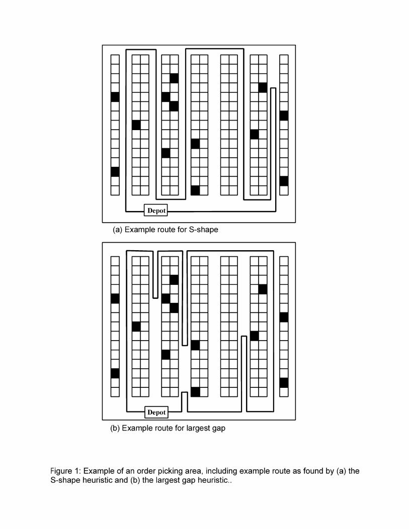
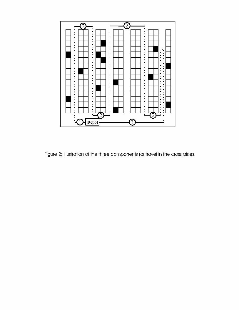
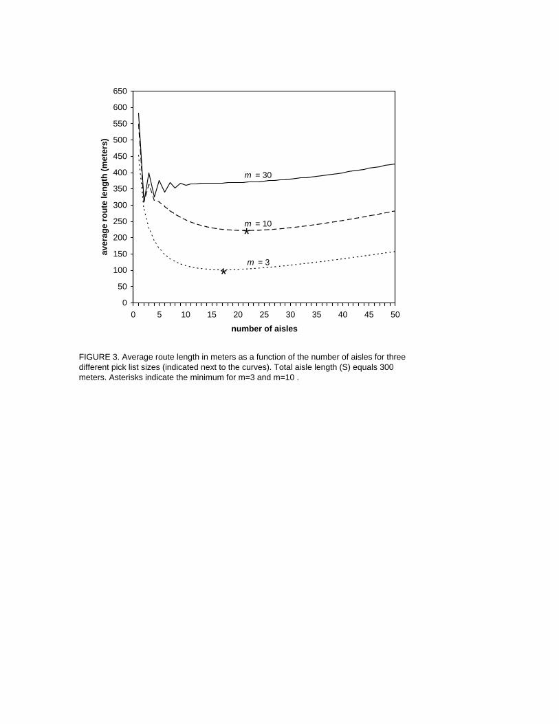
FIGURE 3. Average route length in meters as a function of the number of aisles for three different pick list sizes (indicated next to the curves). Total aisle length (S) equals 300 meters. Asterisks indicate the minimum for m=3 and m=10 .

0

50

100

150

200

250

300

350

400

450

500

550

600

650

0 5 10 15 20 25 30 35 40 45 50

number of aisles

aver

age

rout

e le

ngth

(met

ers)

m = 30

m = 10

m = 3

*

*