a model of complex behavior of interbank exchange...

Available online at www.sciencedirect.com

Physica A 337 (2004) 196–218www.elsevier.com/locate/physa

A model of complex behavior of interbankexchange markets

Tomoya Suzukia ;∗, Tohru Ikeguchib, Masuo SuzukiaaGraduate School of Science, Tokyo University of Science, 1-3 Kagurazaka, Shinjuku-ku,

162-8601 Tokyo, JapanbGraduate School of Science and Technology, Saitama University, 225 Shimo-Ohkubo, Sakura-ku,

338-8570 Saitama-city, Japan

Received 6 January 2004

Abstract

In the present paper, we analyze the complex interaction among three macroscopic variables,dealing time intervals, spreads between ask and bid prices and price movements, observed inactual interbank exchange markets. For this analysis, we propose a new model of interbankexchange dealings as a statistical system integrated by many dealers’ actions with the methodsof statistical physics. For evaluating the plausibility of our model, we compare outputs from theproposed model with the real data by reconstructing a state space with the above three variables,observing ensemble behavior in each day and estimating statistical properties. As a result, wecan con2rm that our model is plausible, and we perform the above analysis with our model fromthe viewpoint of statistical physics.c© 2004 Elsevier B.V. All rights reserved.

PACS: 02.50.Sk; 05.45.Tp; 05.90.+m

Keywords: Econophysics; Exchange market; Spreads; Dealing time intervals; Raster plot

1. Introduction

In recent years, several pioneering studies [1–3] have discussed complex behaviorof 2nancial phenomenon from the viewpoint of statistical physics. Before these stud-ies [1–3] have been published, 2nancial phenomena were not treated as physics, since2nancial phenomena were often considered to be disturbed by dealers’ mind and exter-

∗ Corresponding author. Tel: +81-3-3260-4272; fax: +81-3-3260-9020.E-mail address: [email protected] (T. Suzuki).

0378-4371/$ - see front matter c© 2004 Elsevier B.V. All rights reserved.doi:10.1016/j.physa.2004.01.036

mailto:[email protected]

T. Suzuki et al. / Physica A 337 (2004) 196–218 197

nal information. However, it has been clari2ed that global dealers’ minds and actionsfollow statistical and objective laws [1–3] in an open market even if many dealers tradefreely with sharing almost the same information. Namely, it is very useful to apply theconcepts and methods of statistical physics to 2nancial phenomena. Then, another inter-esting studies have been reported [4–12], which are often referred as Econophysics [13].However, the variety of discussing on 2nancial activities is not wide yet. In particular,

very few discussions have been made on the decision mechanism of bid and ask pricesof dealings in interbank exchange markets, even in the 2eld of economics [14]. Oneof its reasons is that the modeling of this mechanism depends on dealing processes,say in interbank exchange dealings and in stock dealings. While a dealer quotes askand bid price simultaneously in the former, ask and bid price are quoted by diGerentdealers in the latter.Thus if we try to 2nd a general model, which is able to treat both interbank exchange

markets and stock markets, we have to neglect such variables as ask and bid pricesin a model. However, if we focus on making only a model of an interbank exchangemarket, we may use the spread between bid and ask prices. Since these spreads provideimportant information of dealers’ mind of earnings and hedging risks, the movementof the spreads could be one of the essential factors for modeling price movements.In the present paper, we propose a model of interbank exchange dealing by using

not only price movements but also the spreads and the dealing time intervals. In ourprevious study [15], using real data of the interbank exchange market between theSwiss franc and the US dollar, we have already analyzed the interaction among theprice movements, the dealing time intervals and the spreads of real data, and we havediscovered that when the spread becomes larger, the dealing time interval becomesshorter and the movement of price becomes larger [15]. Since the expansion of thespread means that ask and bid prices are separated from the middle price, it is naturalto consider that the dealer tries to sell at higher prices and to buy at lower prices.Such a bull quotation is anticipated to lead to the situation that dealing time intervalsbecome longer when the spread becomes larger, since it is not so easy to 2nd a dealingpartner. However, our analyses [15] show a completely opposite tendency. One of themotivations of the present paper is to construct a novel model which could explainthis remarkable tendency from the viewpoint of statistical physics.The present paper is organized as follows. In Section 2.1, we model the process

of deciding bid and ask prices in the interbank exchange market. In our model, weconsider the distribution of possible future prices by introducing a geometric Brownianmotion [16,17]. Then, we extend it to the distribution from which each dealer expectsfuture prices. In addition, the variance of the distribution corresponds to a Iuctuationterm since dealers’ action is considered as behavior of particles. Next, we formulate thedeciding mechanism of the spread by each dealer. In economics, there is a fundamentalconcept that dealers always act most rationally. Namely, we can naturally consider thateach dealer decides the best spread so that an expected utility is maximized. However,research results of Refs. [1–13] have not used this concept, since it is not so easy totreat or describe such dealers’ mind in a quantitative way. Then, if we consider thereciprocal of the expected utility as a potential energy in physics, the most stable state,that is the best spread, is realized by maximizing the expected utility depending on past

198 T. Suzuki et al. / Physica A 337 (2004) 196–218

information. Thus, in our model, we treat dealers’ mind as a matter with a universalproperty by assuming the natural property that the dealers always act most rationally.In Section 2.2, we make a model for a process of dealing execution in order to decide

dealing time intervals. Here, all dealers are assumed to take part in the model marketwith the formulae proposed in Section 2.1 and 2nd a dealing partner randomly. Whena dealer succeeds in getting a deal with the dealing partner, a dealing time interval isdecided. In Section 2.3, we introduce Auto Regressive Conditional Heteroscedasticity(ARCH) process [18] in order to use it as surrogate data of the price movements.In Section 3, we estimate several statistical properties on the real data in order toshow that the outputs from the proposed model have similar stochastic properties. InSection 4, we show that the same property appears in the data obtained by the proposedmodel and we also discuss the reason why it appears in the proposed model and thereal data from the viewpoint of statistical physics.

2. Proposition of our model

We assume that dealers’ quotations of bid and ask prices are only determined by thepast information. However, in our model we try to consider only the past movementof middle prices between ask and bid prices. Namely, we neglect here the volume ofdealings, not only for the sake of simplicity but also for discussing an essential aspectof complex behavior of price movements.

2.1. Dealers’ action

In this section, we consider a model of the decision mechanism for the spread on thebasis of real dealing action by dealers. First, we formulate the possible future pricesby introducing a geometric Brownian motion [16,17]:

dP(n+ dn) = �(n)P(n) dn+ �(n)P(n) dW ; (1)

where n is a present temporal index, P(n) is a middle price, dW ∼ N (0; dn) andN (0; dn) is a standard normal distribution. Next, we de2ne two coeKcients �(n) and�(n) in Eq. (1) as follows. Let us assume to have the past information of middleprices, which are denoted by P(�), (� = 1; 2; : : : ; n). Here � is the temporal index,that is, � = 1 indicates that it is the 2rst term and P(1) is the 2rst information. Sincethe index n increases one by one whenever each dealing occurs, we consider thatdn = 1. Consequently we have dP(n + 1) = P(n + 1) − P(n). Then, we de2ne �(n)and �(n) by the mean and standard deviations of the movements dP(w)=P(w− 1) (forw= n−p+ 1; : : : ; n), which means the return rates of middle prices during the last pterms.Now, let us introduce two new variables MP and to modify Eq. (1) as

P(n+ 1) = MP(n+ 1) + (n+ 1) dW ; (2)


the movement of middle prices

the distribution A

the distribution B

deciding on

nn

nn

n

n

n

PDd

P

(n n), ( )

Fig. 1. As past information, we only utilize the movement of past middle prices P. The distribution A oGersa possibility of future prices at the (n+1)-th dealing as shown in Eq. (2). The distribution B is an expecteddistribution of a future price by a dealer Dd whose expected value of the future price is MPDd (n + 1) asshown in Eq. (7). The standard deviations of these distributions are described as (n + 1).

whereMP(n+ 1) = �(n)P(n) + P(n) = (�(n) + 1)P(n) ; (3)

which describes the eGect of preserving the trend of price movements, and

(n+ 1) = �(n)P(n) ; (4)

which describes the eGect of maintaining the intensity of price movements. Eq. (2)indicates that there exists a distribution of possible future prices as shown in Fig. 1.We call it the distribution A. The variable MP(n+1) is the mean value of the distributionA and (n+ 1) is the standard deviation of the distribution A.Dividing both hands sides by P(n), Eq. (1) is followed by

dP(n+ 1)P(n)

= �(n) + �(n) dW ; (5)

which means that the return rates follow a Brownian motion. Moreover, since

d logP(n+ 1) = log(P(n+ 1)P(n)

);

= log(P(n) + dP(n+ 1)

P(n)

);

= log(1 +

dP(n+ 1)P(n)

);

� dP(n+ 1)P(n)

; (6)


the return rate means the movement of logarithmic prices. It should be noted thatEq. (6) is the 2rst-order approximation of the Taylor series.Now, we generalize dealers’ actions to model the deciding mechanism of the spreads

between bid and ask prices. In Eq. (2), a best prediction value for the term n + 1surely exists and it is MP(n+1), because it takes the highest probability (of course it isunknown). However, there exists a wide variety of expected prediction values MPD(n+1),which depend on dealers, D={Di; i=1; 2; : : : ; I}, where Di denotes the ith dealer. Thus,in order to model the decision mechanism of prices, we consider these expected bestpredictions MPD(n+1) by the dealers D as follows. Since a future price will be decidedby the predicted price of a dealer who will be able to get a real deal, possible futureprices correspond to the predicted future prices by the dealers D. Thus, the distributionof MPD(n+1) should be the same as the distribution A (the elements of the distributionA are both possible future prices P(n + 1) and the future prices expected by otherdealers D).Now, let us consider dealing actions by dealers included in distribution A. From

Eq. (2), a distribution of future prices expected by the dth dealer (Dd), PDd(n+1), isdescribed by

PDd(n+ 1) = MPDd(n+ 1) + (n+ 1) dW ; (7)

where MPDd(n + 1) is the mean value of the distribution of prediction values by thedealer Dd and (n + 1) is the standard deviation of the distribution, which is a riskfor predicting future price and which is denoted as the same as Eq. (2) for simplicity.Namely, Eq. (7) explains the existence of the distribution B as shown in Fig. 1.

Next, in order to obtain an expected return of one step future at the term n, we tryto calculate expected values of the gain GDd(n + 1) and the loss LDd(n + 1) at theterm n+ 1. It should be noted that GDd(n+ 1) and LDd(n+ 1) depend on bid and askprices quoted by the dealer Dd. We consider K sample variables of the distribution Bof Eq. (7), xDd

k (n + 1) (k = 1; 2; : : : ; K). Since it is very natural for dealers to try tosell at higher prices and to buy at lower prices, we denote the ath “largest” variableof them as an ask price xDd

a (n + 1) and the bth “smallest” variable as a bid pricexDdb (n + 1). Here a = b, since the center of the distribution B is the predicted future“middle” price. Moreover, when the actual future price P(n+ 1) becomes xDd

k (n+ 1),xDda (n+ 1)− xDd

k (n+ 1) or xDdk (n+ 1)− xDd

b (n+ 1) are returns of the dealer Dd.Next, the dealer Dd considers that if P(n+1)= xDd

k (n+1), there exists a predictionerror of MPDd(n + 1) − xDd

k (n + 1) in the distribution B of Fig. 2. Since MPDd(n + 1)and MxDd(n+ 1) are the mean values of the same distribution, MPDd(n+ 1) = MxDd(n+ 1).Then, the prediction error is given by MxDd(n+1)−xDd

k (n+1). Moreover, the dealer Dd

considers that predicted future prices MPD′(n+ 1) by dealers other than the dealer Dd,

D′ = {Di; i= 1; : : : ; I; i �= d}, follows the distribution C shown in Fig. 2. The variableMPD

′(n+ 1) is described by

MPD′(n+ 1) = xDd

k (n+ 1) + (n+ 1) dW : (8)

The meaning of Eq. (8) is that the predicted future prices by dealers D′ distributearound the actual future price xDd

k (n + 1), or P(n + 1), which is a very natural


Fig. 2. A dealer Dd predicts a future price that drops in distribution B. The dealer Dd considers that ifP(n+1)= xDdk (n+1), there is a prediction error between the expected value of the future price MPDd (n+1)and the real future price P(n + 1). Then, the dealer also considers the expected values of the future priceMPD

′(n+ 1) by other dealers D′ (D′ = {Di; i = 1; : : : ; I; i �= d}), which are included in the distribution C as

shown in Eq. (8).

interpretation. Generally, the actual future price corresponds to the mean value of thefuture prices predicted by all dealers.The natural condition that the dealer Dd gets a bid deal or an ask deal with dealers

D′ is given by xDda (n+1)6 MPD

′(n+1) or xDd

b (n+1)¿ MPD′(n+1). That is, the region

where this condition is satis2ed is de2ned by fC(¿ xDda (n+ 1)) or fC(6 xDd

b (n+ 1)).Here, fC is a probability distribution function of the distribution C of Eq. (8). ThediGerence of the mean value between the distributions B and C corresponds to theprediction error of the dealer Dd, MxDd(n+1)− xDd

k (n+1). Then, fC(¿ xDda (n+1)) and

fC(6 xDdb (n+1)) are described by fB(¿ xDd

a (n+1)+ { MxDd(n+1)− xDdk (n+1)}) and

fB(6 xDdb (n+ 1) + { MxDd(n+ 1)− xDd

k (n+ 1)}), respectively. Then, an expected valueof the gain GDd(n+ 1) is calculated as follows:

GDd(n+ 1) =a∑

k=1

1K(xDda (n+ 1)− xDd

k (n+ 1))

×fB(¿ xDda (n+ 1) + { MxDd(n+ 1)− xDd

k (n+ 1)})

+K∑k=b

1K(xDdk (n+ 1)− xDd

b (n+ 1))

×fB(6 xDdb (n+ 1) + { MxDd(n+ 1)− xDd

k (n+ 1)}) ; (9)


where the 2rst term of Eq. (9) is the expected value that the dealer Dd can get anask dealing at a higher price than a real future price xDd

k (n+ 1), or P(n+ 1), and thesecond term of Eq. (9) is the expected value that the dealer Dd can get a bid dealingat a lower price than the real future price xDd

k (n + 1), or P(n + 1). By the symmetryof the distribution, Eq. (9) is reduced to

GDd(n+ 1) =2K

a∑k=1

(xDda (n+ 1)− xDd

k (n+ 1))


k (n+ 1)}) : (10)

In the same way as in Eq. (9), an expected value of the loss LDd(n + 1) iscalculated as

LDd(n+ 1) =K∑k=a

1K(xDdk (n+ 1)− xDd

a (n+ 1))


k (n+ 1)})

+b∑

k=1

1K(xDdb (n+ 1)− xDd

k (n+ 1))

×fB(6 xDdb (n+ 1) + { MxDd(n+ 1)− xDd

k (n+ 1)}) ; (11)

where the 2rst term is the expected value that the dealer Dd gets an ask dealing at alower price than a real future price xDd

k (n+1), or P(n+1), and the second term is theexpected value that the dealer Dd get a bid dealing at a higher price than a real futureprice xDd

k (n + 1), or P(n + 1). Eq. (11) is also reduced to the following equation bythe symmetry of the distribution:

LDd(n+ 1) =2K

K∑k=a

(xDdk (n+ 1)− xDd

a (n+ 1))

×fB(¿ xDd

a (n+ 1) + { MxDd(n+ 1)− xDdk (n+ 1)}

): (12)

Thus, an expected return EDd(n+ 1) at the term n+ 1 is calculated as

EDd(n+ 1)≡GDd(n+ 1)− LDd(n+ 1)

=2K

(K∑k=1

fB(¿ xDda (n+ 1) + { MxDd(n+ 1)− xDd

k (n+ 1)})xDda (n+ 1)

−K∑k=1


k (n+ 1)})xDdk (n+ 1)

)


=2K

K∑k=1


k (n+ 1)})

×(xDda (n+ 1)− xDd

k (n+ 1)) : (13)

It is very natural to assume that dealers will decide bid and ask prices by maximizingEDd(n+1). This maximization corresponds to the fact that it is most stable in potentialenergy where dealers act most rationally as introduced in Section 1. Then, we denote“decided ask prices” by xDd

a (n+1) and “decided bid prices” by xDdb (n+1), and also we

denote the maximized value of EDd(n+1) by EDd(n+1). Moreover, using xDda (n+1)

and xDdb (n+ 1), a decided spread is evaluated as

SDd(n+ 1) = xDda (n+ 1)− xDd

b (n+ 1) : (14)

In the above discussion, we have derived how the dealer Dd decides spreads. Evenif we use another dealer Di instead of Dd, we can discuss in the same way usingEqs. (7)–(14). Namely, EDd(n+1) and SDd(n+1) do not depend on Di (i=1; : : : ; d; : : : ; I)but they depend only on the temporal movement of the standard deviation (n + 1).Thus, we can denote them as E(n+ 1) and S(n+ 1). Then, dealer’s quotations of askand bid prices are

PDia (n+ 1) = MPDi(n+ 1) + S(n+ 1)=2 ; (15)

PDib (n+ 1) = MPDi(n+ 1)− S(n+ 1)=2 : (16)

In order to study the dependence of E(n+ 1) and S(n+ 1) on the standard deviation (n+1), we show the relations between (n+1) and E(n+1) in Fig. 3(a), and between (n+ 1) and S(n+ 1) in Fig. 3(b). For estimating the maximum value of EDd(n+ 1)of Eq. (13), we vary xDd

a by 0:0001 because real prices are rounded oG after the 2fthdecimal place. From Fig. 3, we can con2rm that when (n+1) increases, E(n+1) andS(n+1) increase. In Fig. 3(b), S(n+1) increases discretely by a round-oG eGect. Thiskind of nonlinearity aGects for dealing and dealing time intervals as we will show inSection 3.3.

2.2. The process of dealing execution

In the previous section, we propose a model which decides bid and ask pricesby maximizing EDd(n + 1) using the information on the past movement of middleprices. In this section, we model the process of dealing execution in order to decidedealing time intervals. As introduced in the previous section, the distribution of pos-sible future prices of Eq. (2) corresponds to the distribution of the predicted futureprices MPD(n+1) by dealers D, D= {Di; i=1; 2; : : : ; I}. Namely, the distribution A ofEq. (2) is rewritten by

MPD(n+ 1) = MP(n+ 1) + (n+ 1) dW : (17)

As the rule of interbank exchange markets, the quotation by a dealer, who quotes it toother dealers and can really get a deal, is only recorded as a next price. The quotation


Fig. 3. (a) The horizontal axis is the standard deviation of the expected distribution A. The vertical axisis the maximum of expected returns E. (b) The horizontal axis is the standard deviation of the expecteddistribution . The vertical axis is the decided spread S.

in fail dealing (rejected by a dealing partner) is not recorded. Namely, we can decidethe dealer by referring to a real record of P(n+1). If we denote this dealer by Dl, itspredicted future price satis2es MPDl(n+ 1) = P(n+ 1).From Eq. (7), an expected distribution (the distribution B′ in Fig. 4) of the dealer

Dl, who has P(n+ 1) as a predicted future price, is followed by

PDl(n+ 1) = P(n+ 1) + (n+ 1) dW : (18)

From Eqs. (15) and (16), ask and bid prices are decided by

PDla (n+ 1) = P(n+ 1) + S(n+ 1)=2 ; (19)

PDlb (n+ 1) = P(n+ 1)− S(n+ 1)=2 : (20)

Moreover, each dealing partner of the dealer Dl has a predicted future price in dis-tribution A of Eq. (17). Then, in order to decide a dealing partner of the dealer Dl,we randomly select a variable from the distribution A. If this selected value, which isthe predicted future price of a dealing partner, is larger than the ask price PDl

a or issmaller than the bid price PDl

b , a dealing really occurs with this dealing partner. Here,the probability of getting a deal F(n+ 1) at the term n+ 1 is calculated by

F(n+ 1) = fA(¿PDla (n+ 1)) + fA(6PDl

b (n+ 1)) ; (21)

where fA is the probability distribution function of the distribution A. We iterate thisrandom selection until a dealing really occurs. Once it occurs, we record the number


Fig. 4. We remind that the distribution A is the possibility of future prices and corresponds to the distributionof expected future prices of each dealer as shown in Eq. (17) since a future price is decided by the expectedprice of a dealer who can get a deal. Distribution B′ is the expected distribution of future prices by thedealer Dl who quotes an ask price PDla (n+1) and a bid price PDlb (n+1) to the other dealers and can reallyget a deal at the (n + 1)th term as shown in Eq. (18).

of iterations as the decided dealing time interval !(n+1). By the above processes, weare able to decide the spread S(n+ 1) and the dealing time interval !(n+ 1).

2.3. Approximation of the middle price by ARCH process

Since our aim is to decide dealing time intervals, in order to emphasize the plausi-bility of this deciding process, we take a best way to use the real data of middle pricesfor a next price in the previous section. However, it is also important to consider thecases that the real data of the middle prices are missing. Thus, in the present section,we also discuss the plausibility of our model in the case of using a stochastic processinstead of the real data.In conventional studies to model the price movement, stochastic processes have

often been applied, such as Auto Regressive Conditional Heteroscedasticity (ARCH)[18] and Generalized Auto Regressive Conditional Heteroscedasticity [19] processes.In this section, we apply ARCH process for discussing the case that we cannot usereal movements of middle prices for the proposed model. Thus, even if we do nothave real data, we can simulate the mechanism of producing complex behavior of realmarket data with the proposed model since we need no real data in deciding the dealerDl of the proposed model. 1

1 In the previous section, we discuss how the future spread S(n+1) and !(n+1) can be decided by usingthe real data of P(n + 1) as the future price.


Now, we approximate return rates of middle prices by ARCH process instead ofusing the real data of P(n+ 1) in our model. ARCH(1) is described as

�2(n+ 1) = "0 + "1x2(n) ; (22)

x(n+ 1) ∼ N (0; �2(n+ 1)) ; (23)

where x(n) corresponds to the return rate RP(n)=P(n − 1). If the variance and thekurtosis of return rates are denoted by �2 and #, respectively, "0 and "1 are solved bythe following equations [13]:

�2 ="0

1− "1; (24)

# = 3 +6"21

1− 3"21: (25)

These values are evaluated from the real data [20] as "0=0:8147×10−7 and "1=0:7010,and are used throughout the present paper. Then, the movement of middle prices issimulated by

P(n+ 1) = P(n)√�2(n+ 1)$+ P(n) ; (26)

where $ ∼ N (0; 1).

3. Comparing the model and the real data

3.1. The property of real data

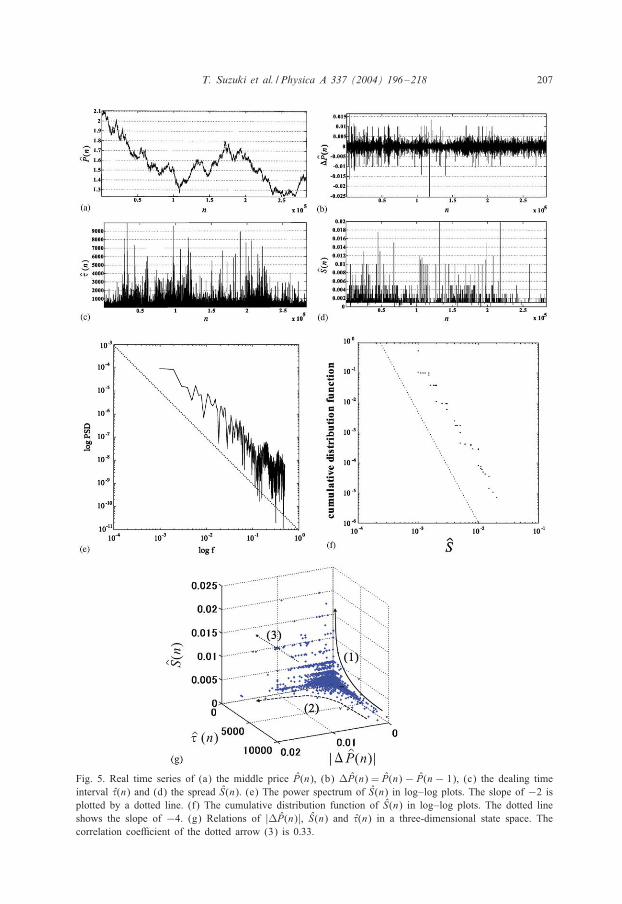
As the real data, we adopt the time series of tick data between the Swiss franc andthe US dollar observed in the interbank market [20]. Figs. 5(a)–(d) show the middleprices, the spread and the dealing time intervals, which are denoted by P (dollars),S (dollars) and ! (s), respectively. 2 The data series are recorded for 1322 days. InFig. 5, n indicates discrete time and it increases one by one with every occurrence ofdealings.In order to examine the temporal dependency of the real spread S(n), we estimate

a power spectrum shown in Fig. 5(e). From Fig. 5(e), we con2rm that the real spreadS(n) has a 1=f−2 type Iuctuation, which means that this temporal dependency is strong.When a probability density function has a power tail, it is well known that the cor-responding cumulative distribution function becomes a straight line in a log–log plot.Fig. 5(f) clearly shows that S(n) has such a characteristic power law.Fig. 5(g) shows the relation among the three variables shown below in a three-

dimensional state space. They denote absolute values of the diGerence of middle prices|RP(n)|, the time interval !(n), and the spread S(n). In Fig. 5(g), there exists therelation that !(n) becomes small when S(n) becomes larger (indicated by the solid

2 We use “∧” for describing real data. For illustration of the proposed model, we use the same variablesthat do not have any additional symbols.


Fig. 5. Real time series of (a) the middle price P(n), (b) RP(n) = P(n) − P(n − 1), (c) the dealing timeinterval !(n) and (d) the spread S(n). (e) The power spectrum of S(n) in log–log plots. The slope of −2 isplotted by a dotted line. (f) The cumulative distribution function of S(n) in log–log plots. The dotted lineshows the slope of −4. (g) Relations of |RP(n)|, S(n) and !(n) in a three-dimensional state space. Thecorrelation coeKcient of the dotted arrow (3) is 0:33.


the arrow (1)). Similarly, the dashed arrow (2) shows that !(n) becomes smaller as|RP(n)| becomes larger. Moreover, there exists a slight correlation between |RP(n)|and S(n) with the correlation coeKcient 0:33 (the relation is indicated by the arrow (3)in Fig. 5(g)). In the case of shuTing these variables randomly, the coeKcient becomesalmost 0, then the value of 0:33 is really signi2cant.

3.2. The property of the data produced from the proposed model

3.2.1. In the case of using the real middle priceFirst, we utilize the real middle price P for the proposed model and calculate the

dealing time interval !′ and the spread S′. 3 We calculate them for 200,000 points with

p = 10. However, since the movement of P(w) (w = n − p + 1; : : : ; n) beyond dailyborders is not suitable for our model, we omit such data from our simulation.We show the time series data obtained from computer simulations in Figs. 6(a) and

(b). Figs. 6(c) and (d) show that S′has the same statistical properties as the real data

S has. Moreover, Fig. 6(e) also shows that there is a similarity between the real dataand the produced data from the proposed model in a state space reconstruction. Thereexists some correlation between |RP(n)| and S ′(n) whose correlation coeKcient is 0:32(the relation is indicated by the arrow (3) in Fig. 6(e)).

3.2.2. In the case of using the middle price simulated by ARCH processNext, we make a simulated middle price P(n) by ARCH(1) in Fig. 7(a) with "0 =

0:8147 × 10−7 and "1 = 0:7010. We show the change RP(n) in Fig. 7(b). Then, weutilize P(n) for the proposed model by p = 10, and calculate the time series dataof !′(n) and S

′(n) that have total 200,000 points. We show these time series data

in Figs. 7(b) and (c) and show statistical properties of S′in Figs. 7(e) and (f). In

Figs. 7(e) and (f), we observe almost the same power law as shown in Figs. 5(e) and(f) and Figs. 6(c) and (d). Fig. 7(g) shows the relation among the three variables inthe three-dimensional state space. In the same way as in Figs. 5(g) and 6(e), we havevery similar results between the real data and our model, namely there is a sort ofdependency indicated by the arrows (1)–(3). Moreover, there exists some correlationbetween |RP(n)| and S ′(n) with the correlation coeKcient 0:28 (the relation is indicatedby the arrow (3) in Fig. 7(g)).

3.3. Discussion on the relation in the state space

In Fig. 5(g), we discover that there exists a sort of dynamical relation among |RP|,S and !. In this section, we discuss why such relations are observed in the results.

First, arrow (1), the relation between S(n) and !(n), is caused by the eGect that realprices, including spreads, are rounded oG after the 2fth decimal place. The reason is

3 We use an extra symbol “′” to each variable, which means that these variables describe the data producedfrom the proposed model.


Fig. 6. (a) The time series data of !′(n) and (b) S′(n) produced by the proposed model with the information

of real data. (c) The power spectrum of S′(n) in log–log plots. The slope of −2 is plotted by a dotted

line. (d) The cumulative distribution function of S′(n) in log–log plots. The dotted line shows the slope of

−4. (e) In the case of using |RP′(n)|, S′(n) and !′(n). The correlation coeKcient of the dotted arrow

(3) is 0:32.


Fig. 7. (a) The time series data of P(n) produced by ARCH(1). "0 = 0:8147 × 10−7 and "1 = 0:7010.(b) The time series data of RP(n). (c) The time series data of !′(n) and (d) S

′(n) produced by the

proposed model. (e) The power spectrum of S′(n) in log–log plots. The slope of −2 is plotted by a dotted

line. (f) The cumulative distribution function of S′(n) in log–log plots. The dotted line shows the slope of

−4. (g) In the case of using |RP′(n)|, S′(n) and !′(n). The correlation coeKcient between !′(n) and S′(n),

the dotted arrow (3), is 0:28.


Fig. 8. (a) The power spectrum of RP(n) in a log–log plot and (b) the power spectrum of |RP(n)| in alog–log plot.

as follows. In the present paper, we simulate S(n + 1) by 0.0001 like a real dealing(as is explained in Section 2.1). Let us denote the rounding error of S(n + 1) by±%(n + 1) and denote the continuous best spread by VS(n + 1). Then, Eqs. (19) and(20) are rewritten as

PDla (n+ 1) = P(n+ 1) + ( VS(n+ 1)± %(n+ 1))=2 ; (27)

PDlb (n+ 1) = P(n+ 1)− ( VS(n+ 1)± %(n+ 1))=2 : (28)

In calculating the occurrence probability of a dealing, F(n+1), in Eq. (21), the roundingerror strongly aGects on F(n + 1) when the standard deviation (n + 1) is small,because the distribution A is a normal one. Moreover F(n+1) increases by −%(n+1)or decreases by +%(n + 1). When VS(n + 1) is small, that is, the standard deviation (n+1) is small, the decrease of F(n+1) by +% is much aGected. Moreover, becausethe dealing time interval !(n + 1) is aGected by F(n + 1), the term +% leads to thereduction of !(n+1). To summarize, for the realization of large !(n+1), it is necessarythat the quantity S(n+ 1) (= VS(n+ 1)± %(n+ 1)) is small. That is, VS(n+ 1) is smallas well.Next, we explain the relation between |RP(n)| and !(n) indicated by arrow (2).

Because the power spectrum of RP(n) shows almost the same property as the whitenoise (Fig. 8(a)), �(n) � 0 and MP(n) � P(n − 1) in Eq. (3). By substituting theserelations into Eq. (17),

MPD(n) � P(n− 1) + (n) dW : (29)

Moreover, since the region RA (in which the probability of dealing realizations ofdistribution A increases) is larger than the region RB (in which the probability ofdealing realizations of distribution A decreases) as the movement of the middle price


Fig. 9. RA is a region in which the occurrence probability of a dealing increases. RB is a region in whichthe occurrence probability of a dealing decreases.

|RP(n)| Iuctuates, it is likely to realize a dealing in a shorter term with small !(n)(Fig. 9). Namely, it is suKcient to reduce !(n) that |RP(n)| becomes large.Finally, we discuss the relation between |RP(n)| and S(n) indicated by arrow (3).

First, recall that the spread S(n) depends on the middle prices in the last p terms{P(n−p); : : : ; P(n− 1)}. When the movement of middle prices in the last p terms islarge, S(n) becomes large as well. Since |RP(n)| has slightly a temporal dependenceas shown in Fig. 8(b), |RP(n)| could take large values too. Namely, there exists apositive correlation between |RP(n)| and S(n). In this reason, we can understand whythere exists the relation among |P(n)|, !(n) and S(n) as shown in Fig. 5(g).

4. Veri�cation of the anomaly with the interbank exchange model

In our previous study [15], we discovered a sort of anomaly from the real data asdiscussed in Section 1. In this section, we show 2rst that such an anomaly could alsoappear in the data produced by the proposed model. Next, we discuss the reason whysuch an anomaly occurs from the viewpoint of the proposed model.

4.1. Raster plot and PSTH of the data obtained by the proposed interbankexchange model

At the beginning, we brieIy review our previous results [15]. In Ref. [15], in orderto analyze interactions of the three variables (P(n); S(n) and !(n)), we use raster plotsand peri-stimulus time histograms (PSTH) [21–23]. These methods are utilized forevaluating the statistical property of neural spike timings in the 2eld of neurophysiologyand provide good schemes to represent spike timings visually.


For example, in order to analyze a response of neural spikes caused by externalstimuli, observed spikes by several trials are plotted along a horizontal axis. In thiscase, these spikes are aligned on each line with adjusting the timing of external stimuli.It is called a raster plot. If there exists a temporal tendency in spike timings, we canvisually recognize it by the raster plots. For further understanding of the ensemblebehavior of spike timings, PSTH can be calculated by transforming raster plots into ahistogram expression.Although the above methods are originally proposed in the 2eld of neurophysiology,

we can expect that both methods can be applied to analyze interbank exchange marketdata since there is a similar aspect between neural spikes and interbank exchangemarket data from the viewpoint that the timings of each occurrence might have essentialinformation. However, there is a signi2cant diGerence between them. For neural spikes,it is widely acknowledged that there is no information in intensities of each spike,because the intensities of spikes become the same due to all-or-nothing property whenthey propagate through axons. On the other hand, for interbank exchange market data,the intensities of each occurrence (spike) have essential information about the prices.Thus, we must analyze the ensemble behavior of the intensities of price movements aswell as timing. Considering the similarity and the diGerence between these two classesof spike information, we modify the methods to be suitable for analyzing interbankexchange market data.In drawing raster plots, we consider the occurrence of actual dealings as spikes, and

each day as a single trial. We also consider the time at which the spread becomes verylarge as time at which external stimuli are applied in order to investigate the responseof market from the movement of spread reIecting dealers’ mind. In addition, since theresponse might depend on a longer temporal eGect due to daily activity, we de2ne fourtemporal sections by dividing the daily dealing time from 9:00 a.m. to 5:00 p.m. (eachsection has 2 h long). Thus, we calculate raster plots and PSTHs by the following dataselection schemes, (i) and (ii), and investigate the existence of response from externalstimuli by comparing both of their results:

(i) In the case that external stimuli are not applied.We randomly select 15 dealing data, in which the actual dealings occur nearly at

the median of each section without any prior information. Here, at the times whenthese dealings occur, the movements of spreads are regular. Then, their dealingsare placed on the vertical line at t=0 on the horizontal axis in raster plots (thoughthe selected 15 dealings are not considered to be applied external stimuli). Here,t describes physical continuous time.

(ii) In the case that external stimuli are applied.We select top 15 dealing data series whose spreads become much larger in each

section. Namely, these dealings are treated as if external stimuli were applied tothem. Then, these dealings are placed as the same as in (i).

If the movement of spreads has no relation with the dealers’ action and does notstimulate the dealers’ action, there is not so large a diGerence between the results bythese two cases that external stimuli are (i) not applied and (ii) applied. However, by


the results of method (ii), we observe that the dealing time interval becomes shorter.In addition, the price movement also shows the diGerence that it has a peak in thetemporal bin at t=0, which means that the expansion of spreads makes the movementof middle prices large.It should be noted that if there exists any expansion of spreads, it indicates that

the ask and bid prices diGer from the middle price. Thus, dealers try to sell at higherprices and/or to buy at lower prices. It is very natural to consider that since it is hardfor such greedy dealers to 2nd a dealing partner, the dealing time interval becomeslonger. In spite of such bull quotations, the dealing time interval becomes shorter. Wecall it an anomaly. We also observe such tendency for the other temporal sections.Namely, it is shown that the expansion of spreads often makes the interval time ofdealings shorter and the movement of prices larger.Now, in order to show that such an anomaly could also appear from the data

obtained by the proposed model, we conduct the following two experiments I and II:

(I) We apply the middle prices of real data to the proposed model in order to obtaindealing time intervals and spreads.

(II) We apply the middle prices simulated by an ARCH process to the proposed modelin order to obtain dealing time intervals and spreads.

We set the temporal bin width as about 30 steps in order to 2t the average values ofPSTH in the previous study [15]. In the jth temporal bin (j = 1; : : : ; J ), dealings aredenoted by sj(m) (m= 1; : : : ; Mj) as shown in Fig. 10, and the average amount of thedaily dealing in each temporal bin is calculated by

Hj =Mj

D; (30)

where D is the number of selected dealing data series in methods (i) and (ii). Thus,we set D= 15. Moreover, in order to examine the average behavior of the movementof middle prices, the movement of the middle price RPsj(m) in the dealing sj(m) isused for calculating the following histogram:

hj =1Mj

Mj∑m=1

|RPsj(m)| ; (31)

where RPsj(m) = Psj(m) − Prj(m), Prj(m) is a one-step previous price of Psj(m) and rj(m)is a one previous dealing of sj(m) as shown in Fig. 10. In Fig. 10, since one previousdealing of sj(m+1) exists in the same bin, rj(m+1)= sj(m). However, if a previousdealing of sj(m) does not exist in the same bin, we set its previous value rj(m) in theprevious bin (the (j − 1)th bin). Then, rj(m) �= sj(m− 1).

4.2. Appearance of the anomaly

Fig. 11 shows the analysis results. In Figs. 11(a) and (b), we show the results inthe case of Experiment (I) (using real data). In Figs. 11(c) and (d), we show theresults in the case of Experiment (II) (using ARCH). With each case of applyingthe middle prices of real data (in Figs. 11(a) and (b)) and simulated data by ARCH


Fig. 10. A raster plot for calculating Eqs. (30) and (31). In the jth bin, the number of dealings is Mj . Then,all dealing timings are numbered from 1 to Mj with the method of raster scanning frequently used in imageprocessing. In the 2gure, rj(m) is one step previous dealing of sj(m). Here, each sequence of dealings isaligned horizontally. Since one step previous dealing of sj(m+1) exists in the same bin, rj(m+1)= sj(m).However, in the case that one step previous dealing of sj(m) does not exist in the same bin, we set itsprevious value rj(m) from the previous bin (the (j − 1)th bin). Then, rj(m) �= sj(m− 1).

process (in Figs. 11(c) and (d)), we can con2rm appearance of the anomaly that theexpansion of spreads makes the interval times short and the movements of middle priceslarge. In order to discuss the reason for the appearance of the anomaly, it is useful touse the discussion on the relation among P, S and ! indicated by arrows (1)–(3) inSection 3.3.First, to discuss the anomaly in hj, we reconsider the relation indicated by arrow

(3) in Figs. 5(g), 6(e) and 7(g). We should remember that the spread S(n) dependson the movement of the middle prices for the last p terms, {P(n− p); : : : ; P(n− 1)}.Therefore, by weak temporal dependence of |RP| shown in Fig. 8(b), there existspositive correlation between S(n) and |RP(n)|. However, when S(n) becomes larger,this anomaly appears. In the proposed model, only the last movement of |RP(n− 1)|makes S(n) larger. Thus, since the memory of the last price movement remains inthe temporal dependency of |RP|, when S(n) becomes larger, the peak showing theincrease of hj appears clearly.Next, we discuss the anomaly in Hj. The anomaly is easily explained by the same

discussion as we used for the relation between |RP(n)| and !(n) indicated by arrow(2). Since the dealing time interval !(n) becomes short when the price movementbecomes large, it is very clear that the dealing time interval becomes short from therelation shown by arrow (2).

4.3. Disappearance of an M type rhythm

In the previous study [15], when we use the 2rst scheme (i), the amount of the dailydealing shows a temporal rhythm whose peak is at about 9:00 a.m. and 3:00 p.m., whichresembles a letter “M” (price movements are almost Iat (no particular rhythms)). Onthe other hand, from the results obtained by method (ii), we have found that many


Fig. 11. The results (a) by method (i) and Experiment (I) (using real data), (b) by method (ii) andExperiment (I), (c) by method (i) and Experiment (II) (using ARCH process) and (d) by method (ii) andExperiment (II).


dealings appear in temporal bins near t = 0 and the large amount of dealings destroysthe rhythm of the shape “M.” Although we can explain why the anomaly occurs inreal data by our model, an M type rhythm cannot be observed in Fig. 11(a).We discuss the reason as follows. In real situations, the number of dealings depends

on the number of dealers who participate in the market. This number always Iuctuatesin the real market. For example, since there exists a diGerence between opening timeand closing time in each bank, the number of dealers who participate in the marketgradually increases in the early morning and it gradually decreases in the evening.Moreover, the number becomes very small at noon because of lunchtime. Namely,since the basic bias, the average number of real dealings in this case, Iuctuates, suchan M-type rhythm appears. However, in the proposed interbank exchange model, sincewe do not consider such a large temporal trend for simpli2cation, the M-type rhythmdoes not appear. However, as in our previous study [15], when the spread becomeslarge (t=0), we can con2rm the reduction of dealing time intervals and the expansionof the movement of prices. Figs. 11(c) and (d) show the results of Experiment (II).The same phenomenon can also appear in this case.

5. Conclusions

In the present paper, we have proposed a novel model of interbank exchange marketson the basis of the three important variables, namely, dealing time intervals, spreads andprice movements. To con2rm the proposed model, we have conducted numerical simu-lations on the real data and the ARCH process (as the movement of middle prices). Wehave shown that the outputs from the proposed model have almost the same statisticalproperties as the real data have. From the viewpoint of the reconstructed state space,raster plots and PSTHs, we have also shown that there exists a possible dynamical rela-tion among the simulated three variables, namely, the movement of prices, the dealingtime interval and the spread. The results shown in the present paper strongly suggestthe plausibility of the proposed model. Namely, this model can make us understandthe characteristic phenomena which are observed in actual interbank exchange marketsand it reproduces complex behavior of price movements. The present results are alsosupported by the fact that the statistical properties of three variables are preserved.Moreover, the other motivation of the present paper is to discuss the anomaly dis-

covered in our previous study [15]. Using the same discussion for the existence ofthe relation among these three variables, we have explained the anomaly on the basisof our proposed model. In addition, we have also shown that we can reproduce theanomaly that is often observed in the real interbank exchange markets, using our pro-posed model by producing the simulated time series of the interbank exchange markets.

Acknowledgements

The authors would like to thanks Prof. Y. Horio and Prof. M. Adachi of Tokyo DenkiUniversity and Prof. K. Jin’no of Nippon Institute of Technology for their valuablecomments and discussions.


The research of TI is partially supported by Grant-in-Aids for Scienti2c Research(C) (No.13831002) from Japan Society for the Promotion of Science, and for Scienti2cResearch on Priority Areas (No.14016002) from Ministry of Education, Culture, Sports,Science and Technology.

References

[1] R.N. Mantegna, H.E. Stanley, Scaling behaviour in the dynamics of an economics index, Nature 376(1995) 46–49.

[2] R.N. Mantegna, H.E. Stanley, Turbulence and 2nancial markets, Nature 383 (1996) 587–588.[3] S. Ghashghaie, W. Breymann, J. Peinke, P. Talkner, Y. Dodge, Turbulent cascades in foreign exchange

markets, Nature 381 (1996) 767–770.[4] H. Takayasu, A.-H. Sato, M. Takayasu, Stable in2nite Iuctuations in randomly ampli2ed Langevin

systems, Phys. Rev. Lett. 79 (1997) 966–969.[5] D. Sornette, Multiplicative processes and power laws, Phys. Rev. E 57 (1998) 4811–4813.[6] L. Kador, Microscopic analysis of currency and stock exchange markets, Phys. Rev. E 60 (1999)

1441–1449.[7] S. Galluccio, Y.-C. Zhang, Products of random matrices and strategies, Phys. Rev. E 54 (1996)

R4516–R4519.[8] L. Laloux, P. Cizeau, J.-P. Bouchaud, M. Potters, Noise dressing of 2nancial correlation matrices, Phys.

Rev. Lett. 83 (1999) 1467–1470.[9] V. Plerou, P. Gopikrishnan, B. Rosenow, L.A.N. Amaral, H.E. Stanley, Universal and nonuniversal

properties of cross correlations in 2nancial time series, Phys. Rev. Lett. 83 (1999) 1471–1474.[10] L.A.N. Amaral, S.V. Buldyrev, S. Havlin, M.A. Salinger, H.E. Stanley, Power law for a system of

interacting units with complex internal structure, Phys. Rev. Lett. 80 (1998) 1385–1388.[11] Y. Lee, L.A.N. Amaral, D. Canning, M. Meyer, H.E. Stanley, Universal features in the growth dynamics

of complex organizations, Phys. Rev. Lett. 81 (1998) 3275–3278.[12] V. Plerou, L.A.N. Amaral, P. Gopikrishnan, M. Meyer, H.E. Stanley, Similarities between the growth

dynamics of university research and of competitive economic activities, Nature 400 (1999) 433–437.[13] R.N. Mantegna, H.E. Stanley (Eds.), An Introduction of Econophysics: Correlations and Complexity in

Finance, Cambridge University Press, Cambridge, 2000.[14] K. Izumi, K. Ueda, Introduction to arti2cial market studies, J. Jpn. Soc. Artif. Intell. 15 (6) (2000)

941–950 (in Japanese).[15] T. Suzuki, T. Ikeguchi, M. Suzuki, Multivariable nonlinear analysis of foreign exchange rates, Phys. A

323 (2003) 591–600.[16] F. Black, M. Scholes, The pricing of options and corporate liabilities, J. Polit. Econ. 81 (1973)

637–654.[17] R.C. Merton, Theory of rational option pricing, Bell J. Econ. Manage. Sci. 4 (1973) 141–183.[18] R.F. Engle, Autoregressive conditional heteroscedasticity with estimates of the variance of U.K. inIation,

Econometrica 50 (1982) 987–1002.[19] T. Bollerslev, Generalized autoregressive conditional heteroskedasticity, J. Econometrics 31 (1986)

307–327.[20] A.S. Weigend, N.A. Gershenfeld (Eds.), Time Series Prediction, Addison-Wesley, Reading, MA, 1993.[21] G.L. Gerstein, M.J. Bloom, I.E. Espinosa, S. Evanczuk, M.R. Turner, Design of a laboratory for

multineuron studies, IEEE Trans. Syst. Man Cybern. 13 (1983) 668–676.[22] J. Krueger, Simultaneous individual recordings from many cerebral neurons: techniques and results,

Rev. Physiol. Biochem. Pharmac. 98 (1983) 177–233.[23] C.M. Gray, P. Koenig, A.K. Engel, W. Singer, Oscillatory responses in cat visual cortex exhibit

inter-columnar synchronization which reIects global stimulus properties, Nature 338 (1989) 334–337.

a model of complex behavior of interbank exchange...

Documents