A Model of Endogenous Extreme Events

Loran Chollete ∗

December 6, 2011

Abstract

Our paper addresses the question ”What determines susceptibility to extremes andduration of extreme episodes?” Extreme events play a large role in recent socioe-conomic life, and in economic models, such as those constructed by Barro (2006),Gabaix (2008), and Wachter (2011). It is therefore important to understand the ex-tent to which the likelihood of extremes depends on behavior of economic agents. Wemodel endogeneity in extremes using the concept of frictions due to congestion, as inthe transaction cost and public good literature. We construct a parsimonious modelof an economy with both financial congestion and positive externalities due to net-work effects. Our model delivers three main results. First, susceptibility to extremesdepends on differences in marginal substitution between net borrowers and lenders.Second, extreme episodes last until marginal substitution rates converge, or expectedcosts rise. Third, a government policy that taxes resource transfers may decrease orincrease the likelihood of extreme events.

Keywords: Endogenous Risk; Extreme Event; Financial Congestion; Network; Public Good

JEL Classification: D62, E44, E51, G01, H41

∗Email loran.g.chollete@uis.no. The author is grateful for support from the Research Council of Norway,Finansmarkedsfondet Grant #185339, and for comments from participants at UiS Business School, the 4thAnnual Conference on Extreme Events, Expectations and Decisions, Norwegian School of Economics andBusiness Administration, Norwegian Central Bank, and Ryerson University.

1 Introduction

’Financial markets...can be quite fragile and subject to crises of confidence. Unfor-tunately, theory gives little guidance on the exact timing or duration of these crises...’Reinhart and Rogoff (2009b), page xil.

The need to understand extreme events in markets has become compelling. This paper develops asimple model of endogenous extremes, based on positive and negative externalities. We address twosalient aspects of modern financial markets: dynamics and endogeneity in extremes. By dynamics,we refer to recurring episodes of ’surprise’ extreme events. By endogeneity, we refer to the effectof economic agents on the likelihood of extremes.1 The economic costs of extreme events can beprohibitive, including widespread risk of default, and an impaired trading process because pricesare uninformative. Extreme events also carry large social and psychological costs, such as the riskof spillovers and increased Knightian uncertainty in an unstable economy.2

Discussions of extreme economic events often model them as generated exogenously.3 But some-times the likelihood of extreme events is affected by behavior of economic agents. Dynamic, en-dogenous extremes occur in economics and in nature, including the effect of human activity on thelikelihood of extreme financial events, and on the natural environment.4 In this paper, we build onexisting literature to explore a possible explanation for endogenous extremes, based on interactionof congestion and network externality effects. Extreme events have externality features, since theyaffect many individuals in the national or global economic system, even though often precipitated bya small number of individuals. It is well known that externalities cause inefficiency of the price sys-tem.5 Consequently, if extreme events are due to externalities, society may not pay the appropriateprice for the extremes that it generates.

Congestion as a Comprehensive Umbrella. A number of researchers have analyzed financial ex-tremes and crises, resulting in a variety of different approaches. Rational approaches discuss bubbleexpectations, agency costs, multiple equilibria, and fire-sale externalities. The financial frictionsapproach emphasizes that liquidity needs at the investor, bank and individual level have aggregate

1Endogenous extremes may arise due to agents’ negligence, bounded rationality, excessive risk taking, orcorruption.

2See Harris (2003), chapter 9; Weitzman (2007); and Caballero and Krishnamurthy (2008). Phelps (2007)emphasizes that a modern economy features endogenous uncertainty due to unforecastability of innovation.For further discussion of financial innovation, see Rajan (2010).

3See Friedman and Laibson (1989); and Barro (2006).4For extremes in economics, see Fisher (1933); Minsky (1982); Grossman (1988); Gabaix et al. (2006);

Allen and Gale (2007); Brunnermeier and Pedersen (2009); and Krishnamurthy (2010). For extremes in na-ture, see Below et al. (2007); and Stern (2007).

5For textbook expositions of externalities, see Varian (1992), and Mas-Colell et al. (1995). For aggregateeffects of externalities, see Blanchard and Kiyotaki (1987); Harrison (2001); and Gabaix (2010a).

1

ramifications.6 Behavioral finance focuses on psychological biases and inefficiencies on the partof banks and individuals. And econophysics research posits that crashes are an emergent propertyof systems with interacting components.7 Several of these research frameworks are presented inTable 1. These multifarious approaches are non-nested and often develop independently of eachother. It is therefore difficult to test models of extreme events or develop policy aimed at mitigatingextremes, in a manner that is credible to economists from different persuasions.

On an empirical level, the various approaches yield mixed results. Figures 1 to 4 illustrate timeseries data on measures of liquidity and investor confidence in the period surrounding large crashesin the Dow Jones Industrial Average (DJIA). Let us focus on the lower panels, which representpercentage changes. We see in Figure 1 that the various measures all experienced concurrent spikeswith the 1987 stock market crash. However, in 1998 during the LTCM crisis there is no strongpattern, as depicted in Figure 2. In Figure 3 we examine the months around Lehman Brothers’bankruptcy in September 2008. Here the liquidity measures display concurrent spikes, but not theconfidence measure VIX.8 Finally, in Figure 4 all measures spike around the date of the flash crashin May 2010. However, the magnitude of changes in this figure (as in all other figures) is very muchlarger than the DJIA itself, which is somewhat puzzling. In order to explore the empirical relationa bit more formally, Table 2 presents rank correlations of the liquidity and confidence measureswith the DJIA. The results are not reassuring. Only the confidence measure VIX is significantlycorrelated with the DJIA. The liquidity measures are not correlated with the DJIA. While theseresults are simple, they underscore that focusing on liquidity (or any single factor) alone may notsuffice to capture the forces behind market crashes.

What can be done to remedy this situation? A possible approach is just to work within one frame-work (e.g. behavioral or frictions) at a time, and build slowly to more general results. Anotherapproach, which we find persuasive, is to look for common ground in all of the theories, that is, toanswer the question ”What, if anything, do the various theories of extreme events have in common?”

A Common Theme. From this perspective, at least one common element emerges: congestionin financial trades. All the above theories are based on the idea that extreme events arise when’too many’ individuals start doing the same activity. The activity is typically one of the following:withdrawing money from banks, selling assets that no longer seem valuable, refraining from buying

6For rational bubbles, agency costs and multiple equilibria, see Blanchard (1979), Bernanke and Gertler(1989), and Benhabib and Farmer (1999), respectively. For fire-sale externalities, see Allen and Gale (2007).For financial frictions and liquidity, see Brunnermeier and Pedersen (2009), Pedersen (2009), and Allen et al.(2011).

7In behavioral finance, Odean (1999) and Barber and Odean (2000b) provide evidence of excess tradingdue to overconfidence; Benartzi and Thaler (1995) discuss implications of myopia for the equity premium;herd behavior is examined by Froot et al. (1992); limits to arbitrage are examined by Shleifer and Vishny(1997). For econophysics research, see Montier (2002) and Sornette (2004).

8VIX is the implied volatility of an at-the-money 30-day option, which reflects investor confidence.

2

assets, demanding margins be repaid, holding on to liquid assets so that entrepreneurs cannot borrowto finance projects. However, if a small enough group of individuals did this action, it would notmatter. There has to be a critical mass for the system to become congested, which then causesmarkets to fail or crash.9 This congestion of the system is consistent with actions that arise becauseof rational beliefs, behavioral biases or any of the other proposed theories of extremes.

In addition to nesting existing theories, this formulation is important because it delivers an importantinsight: it clarifies that extreme events occur not just because agents are acting in a certain way, butalso highlights the importance of system capacity. Just as a large highway can handle more trafficthan a small road, a developed financial market can handle more people selling assets, becauseof another, countervailing effect, network externalities: the more people involved in the market,the greater likelihood of finding counterparties. So market participation brings manifold benefits,especially in the early or middle stages of economic development–entrepreneurs in need of fundingfor worthwhile projects are allowed to borrow and invest in welfare-enhancing innovations. Thislatter perspective is not emphasized in the literature of extreme events and crises. Therefore, thecongestion approach has two advantages. First, it is inclusive and respectful to major frameworksfor modeling extreme events. Second, it provides a way of modeling the important tension betweencosts and benefits of trading resources in financial markets.

How can we formally model congestion in financial markets? There is a mature public financeframework on congestion externalities (Baumol and Oates (1988); Cornes and Sandler (1996)), onwhich we build in the present paper. Consider an economy with I agents, indexed by i = 1, .., I.

As in the public finance literature we model each agent i as buying two types of good, a privateconsumption good yi and a congestible public good qi. In this case the congestible good is thelevel of resource transfers (borrowing, lending, investing or trading) by each agent. If the aggregateamount of the congestible public good is Q ≡

∑i qi, then the likelihood of congestion in the system

is represented by a function C(Q).

Relation to Existing Approaches. The congestion function has an immediate interpretation inexisting theories. In a rational setting, C(·) represents likelihood of experiencing high agency costsor ending up in an inefficient equilibrium. In a behavioral setting, C(·) captures the possibility thatoverconfidence or herd behavior is strong enough to generate excessive trading. And in the frictionsliterature, C(·) measures the likelihood of large, simultaneous liquidity needs in a significant portionof market participants. In sum, our approach attributes extreme events to any major economic factorthat affects the likelihood of congestion. Therefore, it accounts for endogenous extreme eventsregardless of the source–illiquidity, behavioral factors, or rational causes.

9Put differently, as long as the system has enough financial slack to absorb the effect of agents’ actions,financial markets can continue to function smoothly. It is when the actions cumulate to a large enough degree(relative to system capacity) that extreme events occur.

3

1.1 Congestion and Network Effects in Markets

As discussed above, a prominent characteristic of endogenous extremes is congestion: too manyinvestors try to perform the same strategy (e.g. selling an unattractive asset) at the same time, whichsubsequently prevents anyone from using the market. The importance of congested strategies hasbeen explicitly modelled in the literature on herding, liquidity, and information complementarities.10

However, the existence of many investors in a market also has a positive network effect, since itraises the likelihood of finding someone with whom to trade.11 This effect constitutes a socialbenefit of using the financial system to transfer risk and resources. We therefore consider bothcongestion and network effects that may arise due to the presence of market participants.

A Highway Metaphor. It is useful to think of markets as being like highways. In the case of a phys-ical highway, its use allows us to work, consume, invest and live in different places. Consequently,the highway enhances employment of resources for all of society, since it is easier for resourcesto go where they are most needed instead of being locally restricted. Nevertheless, over-use of thehighway also leads to congestion, pollution and other external effects. Highway use therefore con-fers both positive and negative social effects. In the case of markets, they are a virtual highwaywhose use enhances welfare when agents participate, but which is sometimes prone to financialcongestion. Use of this virtual highway, therefore, has both positive and negative social effects.Since congestion externalities have been studied extensively in public economics, we use a simplepublic good framework in our economic model.

As the recent financial crisis has demonstrated, markets can become congested with frighteningspeed and intensity, which precipitates extreme events. In anticipation of Section 2, we use C to de-note the likelihood of extreme events or ’tail risk’, which can affect both real and financial sectors.Previous research has typically modeled this tail risk as an exogenous probability (Barro (2006);Gabaix (2008); Wachter (2011)). It is evidently valuable for both academics and policymakers tounderstand more about determinants of tail risk. One approach (Shin (2009)) is to consider thelikelihood C of extreme events to depend on a reasonable economic variable x, such as excess bor-rowing: that is, the researcher assumes C = C(x), based on economic intuition. While appealing asa starting point, this approach runs the risk of allowing the researcher freedom to choose a tractablebut potentially inaccurate characterization of tail risk. As we show below (in Propositions 4 and 5

10For early references, see Fisher (1933) and Keynes (1936), Chapter 12. For herding research, seeCamerer (1989); Banerjee (1992); Bikhchandani et al. (1992); and Froot et al. (1992). For liquidity, seePedersen (2007); Brunnermeier and Pedersen (2009); Pedersen (2009); and Wagner (2011). For complemen-tarities, see Morris and Shin (1998); Cooper (1999); Vives (2008); and Veldkamp (2011).

11For network externalities, see Katz and Shapiro (1985); Shapiro and Varian (1998); andEasley and Kleinberg (2010).

4

and Corollaries 1 and 2), the optimal C(·) that arises from a micro-founded approach has surprisingproperties and policy implications, which might not be evident based on a priori reasoning.

Our analysis highlights public good features of financial markets. Negative public good aspectshave been examined by a number of authors.12 As discussed above, market participation also con-fers positive externalities. We therefore focus on a public good setting with congestion and networkeffects, to summarize both negative frictions and positive external effects present in modern finan-cial markets. This framework captures two relevant aspects of financial markets. First, during timesof crisis, many investors wish to perform the same type of resource transfer, such as selling badstocks or diversifying. This results in crowded trades, and what is individually rational becomesimpossible for anyone to do (Pedersen (2009); Duffie (2010)). Second, and perhaps more importantfor economic development, in normal times increased use of financial markets is welfare-enhancing,since it loosens intertemporal budget constraints and permits profitable projects to be undertaken.It is only when markets have too large demands placed on them (excess trading, complex securi-ties, etc.) that congestion effects dominate. We use the term financial congestion to denote suchsituations. As shown in Table 1, financial congestion springs from a variety of sources, includingliquidity and frictions, consumer sentiment, excess leverage, and uncertainty about complex securi-ties or new technology. The congestion-network mechanism is always in place, it just has a differenteffect depending on the quality of market use. Since the same forces are at work in normal and badtimes they may in principle be manipulated by public policy.

How does this formulation of endogenous extremes help us? It does so in three ways. First, itallows us to understand the origin of some extremes (the endogenous ones), thereby giving usinsight into which we can plausibly try to avert. Second, it gives banks and regulatory authorities anadditional set of tools from public economics–subsidies, property rights, and so on–that may helpto address extreme events before and during their occurrence. Finally, as noted by Allen and Gale(2007), modern economics does not always show a specific market failure that central banks andregulators can correct by their intervention.13 Our formulation provides a perspective on the role ofgovernment, since it identifies a clear market failure, namely the (positive and negative) externalitiesfrom agents’ neglect to consider their impact on the likelihood of extremes.

1.2 Anatomy of Financial Congestion

Financial congestion arises from various sources, including illiquidity, behavioral biases, excessborrowing and investor sentiment. Focusing on one source alone may not be enough to detect

12See Ibragimov et al. (2009); Acharya et al. (2010a); Acharya et al. (2010c); Shin (2010);Brunnermeier and Sannikov (2011); and Ibragimov et al. (2011).

13See Bernanke and Gertler (2001) for a related discussion.

5

imminent extreme events. In order to illustrate how financial congestion manifests itself and to fixideas, we briefly discuss two simple case studies of extreme events, in 1987 and 2007.

Crash of October 1987. The US stock market crash on October 19, 1987 is a very clear exampleof what financial markets behave like under congestion. Grossman (1988) demonstrated that excessuse of synthetic securities resulted in excess trading which precipitated such crashes. The crash isone of the most significant drops ever seen in stock markets. The size of the drop was tremendous,reflected in all major indices. The DJIA fell 508 points, or 22.6%. The S&P500 also lost more than20% and the Nasdaq fell around 15%. The effect was widespread and affected all types of stocks.Standard large companies like IBM lost around 25% of their value. At the same time, technologystocks like Apple and Intel dropped by around 20% each. Congestion was apparent in the shiftingdirections of aggregate buys and sells. In particular the following pattern was observed:14

• 9:30am. DJIA falls 200 points from 2246 to 2046, shortly after the opening bell.

• 10:00 am. DJIA rises to 2100. This pattern continues throughout the day...

• 2:30 pm. DJIA again at approximately 2100.

• 2:45 pm. Selloff begins, removing 300 more points.

• 4:00 pm. DJIA at approximately 1800 points.

The heavy trading volume was too difficult for computers at the NYSE to keep pace with, so it tookconsiderable time to cumulate all the losses. Eventually the total loss exceeded 500 points, nearlyone-quarter of the DJIA’s value. This and other important market crashes are summarized in Table3.15

2007 Subprime Scare. In the spring and summer of 2007, the aftershock from the subprime market,a relatively small part of US financial markets, reached over to touch hedge funds and internationalmarkets. In the US, credit spreads widened ominously, even for safer debt, and the housing marketreached record breaking levels. In Britain the interbank rate reached its highest level in 9 years.One of the more outstanding examples occurred in July and August of 2007, when hedge funds suf-fered such severe losses that Goldman Sachs, in a one-of-a-kind intervention, had to infuse US$3billion into one of its funds, Global Equity Opportunities. This fund lost 30 per cent of its value inthe week between August 3 and August 10, 2007. A major reason cited for the severe hedge fundlosses was that the extremes occurring in markets were ’25 standard deviation’ events (New York

14This account of the 1987 crash summarizes material in Sornette (2004).15We include only the USA and Hong Kong, because both countries have liberal capital markets, with few

restrictions on investing and transferring capital overseas. Thus the extreme events are not due to governmentintervention but to competitive market forces.

6

Times, August 13, 2007). The incidents are puzzling because hedge funds did not seem directlyexposed to heavy enough risk to warrant such drops in value. Moreover, most large investors haverisk management systems that are stress tested against extreme market events such as terrorism risk,banking crises, and interest rate changes. So what sort of event could surprise such respected in-vestors enough to lose as much as one-third of their value? A potential answer is that our approachto understanding surprise extreme events is incomplete. This incompleteness may stem from thefact that both information economics and current risk management are generally silent about endo-geneity in the likelihood of extremes.

In light of the preceding observations, we analyze extreme events that are dynamic and endogenous.It should be noted that a type of endogeneity is recognized in certain spheres of risk analysis. In-formation economics acknowledges that individual agents’ behavior can affect individual outcomesin settings such as insurance markets. However, this framework is usually restricted to individualagents or sectors, and typically requires asymmetric information between borrowers and lenders.16

In our model, we illustrate that endogenous risk effects can spill over to other sectors even in theabsence of asymmetric information. A graphical depiction of our approach is in Table 4, whichshows that our view of endogenous probability nests that of moral hazard. The difference is that weconsider broader settings, encompassing spillovers and general information structures.

1.3 Related Literature

Our research relates to existing work on extreme events, coordination externalities, liquidity, andsystemic risk. Regarding extreme events, Mandelbrot (1963) and Fama (1965) show that US stockreturns are not gaussian and have heavy tails. Fama (1965) also documents that stock crashes oc-cur more frequently than booms. Jansen and de Vries (1991) investigate the distribution of extremestock prices in S&P500 stocks, and document that the magnitude of 1987’s crash was somewhatexceptional, occurring once in 6 to 15 years. Susmel (2001) uses extreme value theory to investigateunivariate tail distributions for international stock returns. He documents that Latin American mar-kets have significantly heavier left tails than developed economies. Empirically, it has been shownthat investors and assets tend to behave similarly during extreme periods, which also motivatesthe congestion approach. In this regard, Longin and Solnik (2001) use a parametric multivariateapproach to derive a general distribution of extreme correlation. The authors examine equity in-dex data for G5 economies and document that correlations are significant in the left tail of returns.They also show that correlations increase during market downturns. Hartmann et al. (2003) doc-

16The 2007-2009 financial crisis, however, affected numerous sectors and regions. Moreover, for subprimemortgages it is difficult to apply standard information economics. To do so, one must argue that poor qualityof the subprime borrowers was ’hidden information’, and that lenders did not understand the potential fordefault when supplying loans to borrowers with poor credit history or no collateral.

7

ument that Latin American currencies have less extreme dependence than in east Asia, and thatdeveloping markets often have a smaller likelihood of joint extremes than do industrialized nations.Hartmann et al. (2004) report that stock markets crash together in one out of five to eight crashes,and that G5 markets are statistically dependent during crises. Poon et al. (2004) model multivariatetails of stock index returns from G5 markets. They document that in only 13 of 84 cases is thereevidence of asymptotic dependence. They argue that the probability of systemic risk may be over-estimated in financial literature. Chollete et al. (2009) use general dependence measures to modelportfolios of international stock returns from the G5 and Latin America. They find that an em-pirical model that allows for asymmetric dependence outperforms standard models, and improvesValue-at-Risk computations. In a comprehensive study of more than 800 years of financial crises,Reinhart and Rogoff (2009b) conclude that the biggest factors in crises are excessive debt and sud-den shifts of confidence. During booms, governments, banks or corporations increase borrowing,and underestimate aggregate risk. The authors emphasize a ”This time is different” mentality, wheremarket participants downplay the likelihood of extreme events during the boom period precedingcrises. Adrian and Brunnermeier (2010) construct a measure, CoVaR, that summarizes the con-ditional likelihood of an institution’s experiencing a tail event, given that other institutions are indistress. They estimate CoVaR for commercial banks, investment banks and hedge funds in the US,and document statistically significant spillover risk across institutions. Theoretical work on extremeevents also supports the idea of endogenous extremes due to congestion. In this regard, Montier(2002) discusses the notion that crashes and outliers are endogenous, perhaps due to a preponder-ance of sellers relative to buyers. Danielsson and Shin (2003) model a scenario where unanticipatedcoordination of agents’ behavior leads to an endogenous increase in risk. Liu et al. (2003) demon-strate in a jump diffusion setting that consideration of rare events discourages individual investorsfrom holding leveraged positions. Bazerman and Watkins (2004) suggests that certain ’surprise’events in modern society are predictable, since there may exist sufficient information to know thatthese events are imminent. Liu et al. (2005) develop an equilibrium model of asset prices withrare events. The authors document that aversion to rare events can ameliorate option mispricing.Gabaix et al. (2006) develop a theory of stock volatility, where the driving force is trading by largeinvestors, during illiquid markets. Barro (2006) builds a representative agent economy that incorpo-rates the risk of a rare disaster, modelled as a large drop in the economy’s wealth endowment. Whenthis model is calibrated to the global economy, it can explain the equity premium and low risk freerate puzzles, and helps account for stock market volatility. Weitzman (2007) constructs a Bayesianmodel of asset returns. He discovers that when agents consider the possibility of extremes, there isa reversal of all major asset pricing puzzles. Gabaix (2008), Gabaix (2010b), and Wachter (2011)generalize the Barro framework to account for dynamic probability of extreme events. These lattermodels can explain outstanding macroeconomic and finance puzzles as well as the behavior of stockvolatility. Bollerslev and Todorov (2011) use high frequency options data to construct an index of

8

implicit disaster fears among investors. The authors’ method helps to explain patterns in the eq-uity premium and stock market variance. These papers all underscore the importance of accountingfor extreme events in markets. None of the papers, however, analyzes the endogenous causes of dy-namic extreme events. This lack of research on endogenous extremes serves as a primary motivationfor our paper.

Regarding coordination externalities, Bikhchandani et al. (1992) and Banerjee (1992) build mod-els of how agents may coordinate and disregard their private information. Such herd behavior haseffects on the stock market, as examined by Froot et al. (1992). Allen and Gale (1998) constructa model of banking panics that are related to the business cycle. In this model depositors mayrationally fear low returns on their deposits after observing that leading economic indicators sug-gest a downturn, and therefore optimally withdraw all funds from banks. The authors show thatbank runs can be efficient, although this result does not hold when runs lower asset returns, nor inthe presence of a stock market. In their Theorem 5 and Corollary 5.1, the authors formalize theinefficiency of bank runs, which motivates central bank intervention. Aggregate consequences ofexternalities have also been modelled by Blanchard and Kiyotaki (1987); Cooper (1999); Harrison(2001); and Veldkamp and Van Nieuwerburgh (2010). A related literature on bubbles suggests ex-treme events can be caused by rational indeterminacy, behavioral factors, or new technology, asdiscussed by Blanchard (1979), Abreu and Brunnermeier (2003), and Hong et al. (2008), respec-tively. Allen and Gale (2007) show that bubbles may be precipitated by incentive and limited liabil-ity issues, which reduce the costs of individual risk taking. In chapter 7 of Allen and Gale (2007)the authors suggest there is not always a clear market failure for regulators to correct, in the caseof market instability. This latter point motivates our paper to develop a framework that formalizesmarket failures inherent in extreme events. We recently became aware of papers by Bianchi (2010),Bianchi (2011) and Bianchi and Mendoza (2011), who analyze dynamic equilibrium models whereexcess borrowing increases financial system fragility. The authors show that these negative external-ities raise the likelihood of extreme events, and entail significant welfare costs in terms of foregoneconsumption. Bianchi (2011) suggests that increased borrowing costs during tranquil periods maycorrect the externalities. The above papers do not consider the interplay between negative and pos-itive externalities from resource transfers, which motivates our paper.

Regarding liquidity, Brunnermeier and Pedersen (2009) demonstrate that liquidity needs at the mar-ket and funding level can be self-reinforcing. During bad times, such liquidity needs can precipitatefinancial crises. Pedersen (2009) describes a situation where major market players all require liq-uidity, which ends up causing a shutdown in markets. Similar frictions can arise in markets wherecapital is deployed in a sluggish manner, and when there is a discrepancy between sophisticatedand naive investors, see Duffie (2010) and Stein (2009). Wagner (2011) demonstrates that wheninvestors face liquidation risk in multiple assets, they hedge by selecting heterogeneous portfo-

9

lios with lower diversification benefits. These papers correctly emphasize the importance of trans-action costs and liquidity in market outcomes. However, as shown in Tables 1 and 5, extremeevents may occur because of other factors such as excessive government debt and confidence shifts(Reinhart and Rogoff (2009b), and Keynes (1936)) or over-borrowing in the financial sector (Fisher(1933)). Moreover, liquidity is notoriously very difficult to measure (Aitken and Comerton-Forde(2003); Sadka and Koracjczyk (2008); and Goyenko et al. (2009)). Finally, the results in Table 2show that liquidity does not always convincingly relate to stock market changes during extremeperiods. Thus, a focus on liquidity may ignore other important determinants of endogenous extremeevents. Expanding the focus of the liquidity literature (with respect to extreme events) provides afurther motivation for a general congestion approach.

Regarding systemic risk, Danielsson and Zigrand (2008) construct an equilibrium model where as-set prices are determined in the presence of systemic risk. The authors argue that while regulationcan reduce the likelihood of systemic risk, it carries costs, such as increased risk premia and volatil-ity, and the possibility of non-market clearing. Acharya et al. (2010a) describe the causes of thefinancial crisis of 2008, arguing that a key catalyst was excessive leverage, which created systemictail risk. Acharya et al. (2010b) construct a measure of systemic risk tendency, SES, based on co-movement of expected shortfall of individual institutions and the aggregate financial system. Theydemonstrate ex ante predictive power of SES for various companies during the period 2007-2009.Acharya et al. (2010c) develop an approach to regulating systemic risk based on SES. They proposethat financial firms be taxed proportionally to their expected loss in the event of a systemic crisis.On the theoretical side, Embrechts et al. (2002) and Ibragimov and Walden (2007) show that whenportfolio distributions are heavy-tailed with nonlinear dependence, they may result in limited diver-sification. Shin (2009) demonstrates a wedge between individual risk and systemic risk, based onthe tendency of agents to coordinate during extreme periods. A similar result based on heavy tails isproven by Ibragimov et al. (2009); and Ibragimov et al. (2011). Thus, there are aggregate economicramifications for heavy tailed assets, since individuals’ diversification decisions yield both individ-ual benefits and aggregate systemic costs. If systemic externality costs are severe, the economymay require intervention to improve resource allocation. Morris and Shin (2011) develop a modelwhere adverse selection is amplified across market participants when agents cannot compute maxi-mal expected losses. None of these papers examines endogeneity of tail risk where both positive andnegative externalities are accounted for. This provides a final important motivation for our paper.

1.4 Contribution of our Paper

Our paper contributes to the literature in several respects. First, unlike previous research, we charac-terize the endogenous probability of extreme events, using a micro-founded approach. Specifically,

10

we derive mathematical expressions to characterize the ’signature’ of dynamic, endogenous ex-tremes. Second, we account for both positive and negative externalities in financial markets, withinthe same model. Third, our model demonstrates the conditions where government intervention isand is not justified in the face of extreme events. More generally, our framework allows us to discussan economic approach to extreme events, using the lens of public economics. The remainder of thepaper is organized in the following manner. Section 2 constructs a simple model of endogeneity ofC, using a congestible public good framework. Section 3 develops this model to characterize dy-namic, endogenous extremes in a model of resource transfers between agents. Section 4 concludes.

2 Endogenous Extremes: Financial Congestion and Net-works

A larger network means a smaller worldDelta advertisement

We model endogeneity of extremes as arising due to congestion effects. Extreme probabilities canbe exogenous or endogenous, each with a different policy response.17 Exogenous extremes arrivefrom outside the economic system and are truly acts of nature, from the perspective of the domesticeconomy. For example, in a crop-based economy, the probability p of extreme changes in cropvalue could depend on exogenous swings in weather.18 Since weather is generally unpredictablebeyond a few days, and exogenous to an individual farmer, in this case the probability of extremesis essentially random. Endogenous extremes, by contrast, are generated and amplified within theeconomic system, by agents’ activity and interaction. This activity persists because extremes haveexternality-like attributes, and therefore agents ’over-produce’ the amount of extremes in the sys-tem. Several alternative approaches are presented in Table 5. For example, stock market crashesand banking panics may stem from excessive risk taking and borrowing of a segment of the econ-omy (Fisher (1933)), excessive credit creation (Allen and Gale (2000)), and excessive reliance oncomputer-based trading (Grossman (1988)).19 Since each agent has an incentive to borrow or risktoo much from the social point of view, competition leads to overproduction of extremes. As dis-cussed above, this congestion effect balances against a countervailing network effect, since market

17 In practice, there is a spectrum of extremes, with some being a mixture of exogenous and endogenous.The tools developed herein help us to assess the dominant influence on extremes.

18Other causes of exogenous extremes include foreign wars, natural catastrophes, and uncertainty aboutnew technology.

19The above authors consider some form of extreme event or crisis, but vary in their emphasis on endo-geneity. Our paper seems to be the first to use this framework explicitly in a general setting.

11

participation increases social welfare. Hence, the probability of extremes may no longer be random.We develop the relevant expression for endogenous extremes below.

While exogenous extremes are statistically unrelated to the economic environment, endogenousextremes (since they are generated by economic agents) should reflect optimizing or equilibriumbehavior of agents. We focus on a canonical form of economic interaction, namely transfer ofresources.20 The heart of the externality is as follows. A key feature of modern financial markets isthat they enhance agents’ ability to transfer resources, which involves either trading commoditiesand assets or moving assets across time. This transfer of resources can aid or harm other individualsnot party to the transfer. For example, massive stock sales by some investors can decrease the stockprice, thereby increasing market volatility and diminishing portfolio values of all other investorswho own that stock.21 In similar vein, excessive borrowing by a relatively small set of investorscan increase the likelihood of a systemwide market crash.22 On the positive side, increased marketparticipation makes it easier for investors and borrowers to find counterparties due to thick marketeffects. This is true domestically as well as internationally, since emerging economies with excesssavings can channel their surplus to developed countries and loosen their budget constraints. Hencethe behavior of individual agents inherently affects the wellbeing of others without being reflectedin a price–the definition of an externality. In sum, modern markets confer ability to transfer financialresources easily, but may bear hidden costs and benefits in the form of externalities.2324 Even thoughagents realize their collective behavior affects market thickness and the likelihood of extremes, theymay persist in myopic behavior, since they do not bear all costs and benefits.

2.1 A Model of Financial Congestion

We consider a stylized model where agents use financial markets to transfer idle resources to thepresent from the future, or from one resource-plenty agent to a resource-scarce agent. Agents partic-

20Resource transfers include such activities as borrowing funds, and trading assets. Resource transfers areessential functions of financial markets, see pp. 4-7, Goetzmann and Rouwenhorst (2005).

21See Gabaix et al. (2006).22Fisher (1933), Minsky (1982), Montier (2002), and Allen and Gale (2007) discuss the fact that large

asset price and output fluctuations for the entire economy may result from various forms of resource transferswithin specific sectors–increased trading, increased desire to liquidate assets, and increased borrowing.

23The externality costs of large resource transfers for an individual depend on the dominant social attitudetowards transfers at the particular time. Thus, there might be zero or even negative perceived costs of trans-ferring resources during the upswing in asset cycles. There is also evidence of different attitudes by the sameindividuals at different stages of their life cycles, see Agarwal et al. (2007). For related ideas, see Minsky(1982); Kiyotaki and Moore (1997); Baker and Wurgler (2007); and Bansal and Shaliastovich (2010). Forresearch on the leverage cycle, see Fostel and Geanakoplos (2008).

24We focus on the likelihood of extremes. For work on the structure of specific extreme events, seeAbreu and Brunnermeier (2003); Hong et al. (2008); and Reinhart and Rogoff (2009a). For work discussingrational individuals’ perception of extreme risk, see Weitzman (2007).

12

ipate in the financial market, which has elements of the commons, but also another aspect, individualcontribution: participating in the market generates more thickness and a better chance of matchingand diversification.25 Therefore an agent who participates in resource transfers faces 3 effects. Sheenhances her own utility; she contributes to decreased performance of the system whenever sheexcessively coordinates with others’ trading strategies (negative congestion externality); and shehelps improve functioning of the system by enlarging trade possibilities for others (positive networkexternality).

Hence at the aggregate level resource transfers result in a tension between enhancing thick marketsversus avoiding congestion. We therefore build a simple model of financial congestion, where someuse of financial intermediaries yields positive network effects but excess use results in reduction orremoval of ability to trade. To formalize our approach we build on the public economics literatureon congestion (Baumol and Oates (1988); Cornes and Sandler (1996); Myles (1995)) and use twodistribution functions: the congestion function C(·), which measures the distribution of congestedtrades in financial markets, and the network function N(·), which summarizes enhanced tradingopportunities due to thicker markets.

The Environment. The economy E is defined as a collection of goods (q, y), prices π and pref-erences U , that is, E = (q, y, π;U(·)). Specifically, U(·) is a utility function, y is a consumptiongood, q represents resource transfers; and π represents average prices. The environment comprisesI ≥ 2 identical individuals of whom we consider one representative individual. Each agent i buysa consumption good yi and also trades qi units of her resources. The total amount of trading is∑I

i=1 qi ≡ Q, which affects the likelihood of congestion or friction in financial markets. Thus Q is

a public good that negatively affects utility, since it raises the likelihood of socially harmful extremeevents. Each agent has an exogenous income W i, and takes as given the prices of y and q, namelyπy and πQ. We normalize the price of y to πy = 1.

Assumptions and Definitions. Agent’s preferences are represented by a neoclassical utility func-tion U as in Allen and Gale (2007). U(·) is therefore quasi-concave, increasing and continu-ously differentiable.26 U depends on goods, congestion C and network effects N , that is, U =

U(y, q, C(·), N(·)). As in the public economics literature (Baumol and Oates (1988); Cornes and Sandler(1996)) congestion depends on aggregate usage Q, that is, C = C(Q). Thus, the likelihood of con-gested trades depends on the level of resource transfers in the economy. Throughout, we restrictattention to interior optima for illustrative purposes. Derivatives are denoted with a subscript. Forexample, Uy ≡ ∂U

∂y , Uq ≡ ∂U∂q , and Uc ≡ ∂U

∂c . Similarly, CQ ≡ ∂C∂Q , and NQ ≡ ∂N

∂Q .

25For work on thin markets, see Rostek and Weretka (2010) and Rostek and Weretka (2011).26For definitions and implications of quasi-concavity, see Mas-Colell et al. (1995).

13

Assumption 1. The derivatives of the congestion and network functions satisfy NQ ≥ 0 and CQ ≥ 0.Thus, an increase in total resource transfers always (weakly) increases both the network effect andthe likelihood of congestion.

Assumption 2. The derivatives of the utility function satisfy UN ≥ 0 and Uc ≤ 0. Thus, an increasein market thickness weakly increases utility, while an increase in congestion weakly decreases util-ity.

Assumption 3. For congestion to occur, at least two agents must use the markets. Thus, in a two-person economy, C(0, ·) = C(·, 0) = 0. This rules out cases where an autocrat can shut downmarkets unilaterally.

Definition 1: An extreme event is a large drop in average prices π.

Definition 2: An exogenous extreme event occurs when a large fall in asset prices is unrelated toany economic variable v ∈ E.

Definition 3: An endogenous extreme event occurs when a large fall in asset prices is related tosome economic variable v ∈ E.

Since endogenous extremes arise because of congestion in our model, the likelihood of an endoge-nous extreme event is given by the derivative of the distribution function, that is, by CQ. Below, weconsider 2 cases in turn: markets exhibit only congestion effects, and markets have both congestionand positive network effects.

2.1.1 Financial Markets Exhibit Only Congestion Effects

In this setting, there is no aggregate benefit from market participation, there is only individual benefitto the agent. Thus, the market is just a facility like a recreation area that yields pleasure to eachindividual that uses it, but accords no systematic benefit for society as a whole. Moreover, there arenegative external effects–sometimes the market gets congested, which causes extreme events thatnegatively affect all society. The representative individual has a quasi-concave utility function

U i(·) = U i(yi, qi, C(Q)), (1)

14

where C(Q) is a congestion function with the properties CQ ≥ 0, and Uc ≤ 0. That is, the likelihoodof congestion increases as resource transfers increase; and the agent’s utility falls if congestionbecomes more prevalent.27

Private Optimum: The representative individual chooses her level of resource transfers, in a Nash-Cournot setting, where she takes Q =

∑j =i q

j as exogenously given. Her problem is

max(yi,qi)

U(yi, qi, C(Q+ qi))

subject toyi + πQq

i = W i.

The first order necessary conditions for interior optima imply U iq+U i

cCQ

Uy= πQ, which can be ex-

pressed in terms of the likelihood of congestion:

CQ =πQ−

U iq

U iy

U ic

U iy

. (2)

According to (2), the likelihood of congestion is proportional to the difference in the marginal costand benefit of an additional resource transfer. We now turn to the social optimum.

Social Optimum: If we consider a simple equal weighting of utilities, the corresponding socialproblem is

max(yi,qi)

∑i

U i(yi, qi, C(Q))

subject to ∑i

yi + πQ∑i

qi =∑i

W i,

The first-order necessary conditions are U iy − λ = 0 and U i

q +(∑

j UjC

)CQ − λπQ = 0. These

combine to yield U iq

U iy= πQ −

∑j

(UjC

U iy

)CQ, or

U iq + U i

CCQ

U iy

= πQ −∑j =i

(U jc

U iy

)CQ.

27This formulation of congestion is standard in public economics, see Baumol and Oates (1988); andCornes and Sandler (1996). q can be, for instance, the amount of public good related to trading in credittransfers by financial market participants.

15

The above expression is intuitive: at the optimum agent i’s marginal valuation of additional resourcetransfers q equals the marginal private cost πQ plus the social cost associated with increasing ex-treme congestion in the financial system. To focus on extremes, we rewrite the above expression as∑

j

(UjC

U iy

)CQ = πQ − U i

q

U iy

, which implies

CQ =πQ − U i

q

U iy∑

j

(UjC

U iy

) . (3)

Equation (3) says that at the social optimum, the marginal likelihood of congestion CQ equals themarginal private cost minus the marginal benefit agent i places on additional (congestion-causing)resource transfers.

When is the likelihood of congestion larger? By comparing (2) and (3), we see that the privatesolution CQ is larger. This is true because the denominator does not account for all economy-wide marginal rates of transformation. Intuitively, when she does not have to account for her extracongestion effects, each agent will over-use the financial system.28 Thus for a given level of re-sources, the likelihood of congestion is larger when agents act competitively and do not considercongestion externalities. This result provides an asset market counterpart to the banking result ofAllen and Gale (1998) (Corollary 5.1). We summarize it in the following Proposition.

Proposition 1. In an economy with congestion effects due to resource transfers, the likelihood ofcongestion in a competitive market is larger than in the social optimum.

Proof: By inspection of (2) and (3). �

2.1.2 Financial Markets Exhibit Congestion and Network Effects

We now consider a more realistic environment, which is the focus of our analysis in the paper. Theenvironment is one in which individual and social welfare are affected by both congestion and posi-tive externalities. The positive externalities reflect ease of finding counterparties and diversificationwhen markets are thicker, and also reflect the overall quality of the financial network N available(see Shapiro and Varian (1998); Easley and Kleinberg (2010)). The overall quality of markets de-pends on total trading activity Q, which is contributed to by each new participant that comes to themarketplace to conduct resource transfers. In order to capture this network effect we include a net-work function N(Q). The representative utility function may be written as U i(yi, qi, C(Q), N(Q)),

28Overuse involves excess trading, or any economic activity that generates excessively high informationaldemands on the system.

16

where the derivatives satisfy NQ ≥ 0, and UN ≥ 0. Thus, an increase in resource transfers increasesnetwork quality, and utility increases with network quality. We can now expand the above discus-sion of negative externalities to consider optimal social benefits that come from thicker markets,enhanced liquidity and trading opportunities, due to investors’ participation in the financial system.

Private Optimum: The representative individual takes Q =∑

j =i qj as exogenously given, so her

problem ismax(yi,qi)

U(yi, qi, C(Q+ qi), N(Q+ qi))

subject toyi + πQq

i = W i.

The first order conditions are U iy − λ = 0 and U i

q + U iCCQ + U i

NNQ − λπQ = 0, which combineto give

πpQ =

U iq + U i

NNQ

U iy

+U iC

U iy

CpQ, (4)

or

CpQ =

πpQ − U i

q+U iNNQ

U iy

U iC

U iy

, (5)

where the superscript p denotes a private solution. CpQ measures the likelihood of congestion-caused

extreme events in a competitive economy, and is an important quantity which we shall use in Section3 below.

Social Optimum: The corresponding social optimum solves the following program:

max(yi,qi)

∑i

U i(yi, qi, C(Q), N(Q))

subject to ∑i

yi + πQ∑i

qi =∑i

W i.

The necessary first order conditions are U iy −λ = 0 and U i

q +∑

j UjCCQ+

∑j U

jNNQ−λπQ = 0,

which together yield

πsQ =

U iq +

∑j U

jNNQ

U iy

+∑j

(U jC

U iy

)CsQ, (6)

or

CsQ =

πsQ − U i

q+∑

j UjNNQ

U iy∑

j

(UjC

U iy

) , (7)

17

where the superscript s denotes the social optimum. CsQ is the likelihood of congestion-caused

extreme events in an economy where social costs are considered. Importantly for both the social andcompetitive optimum, the likelihood of extremes is negatively related to network effects, becauseboth congestion and networks depend (in opposite ways) on aggregate resource transfers Q. Wesummarize this in the following Proposition.

Proposition 2. Consider an economy with external congestion and network effects due to resourcetransfers. At an interior optimum, the (private and social) likelihood of extreme events increases asthe marginal network effect falls. That is, CQ is inversely and monotonically related to the networkeffect NQ.

Proof: By inspection of (5) and (7). �

While the result in Proposition 2 follows directly from the calculus of networks and congestion,it is instructive because it explicitly relates the countervailing forces that have to be reckoned withwhen designing public policies aimed at increasing market thickness and liquidity, in order to reduceexposure to extremes. Focusing on the competitive equilibrium (5), we see that the relation betweencongestion Cp

q and networks NQ is nonlinear in general. Consequently, the probability of extremesdepends on the level of financial market participation in a monotone, but potentially nonlinear way.

When do private markets yield inefficiently high levels of endogenous extreme events? Comparisonof conditions (5) and (7) reveals that the private likelihood of congestion Cp

Q exceeds the socialoptimum Cs

Q if the following inequality holds:

πpQ

U iy

U ic

−U iq + U i

NNQ

U ic

> πsQ

∑j

(U iy

U jc

)−

U iq +

∑j U

jNNQ∑

j Ujc

.

Given the assumption of I identical individuals, superscripts can be removed to yield U i = U j = U,

and∑

j UjC = IUC . Therefore the above inequality can be rewritten as

πpQUy − Uq − UNNQ

UC>

πsQUy − Uq − IUNNQ

IUC,

orIπp

QUy − IUq − IUNNQ − πsQUy + Uq + IUNNQ

IUC> 0,

which simplifies toIπp

Q − πsQ

I − 1>

Uq

Uy.

18

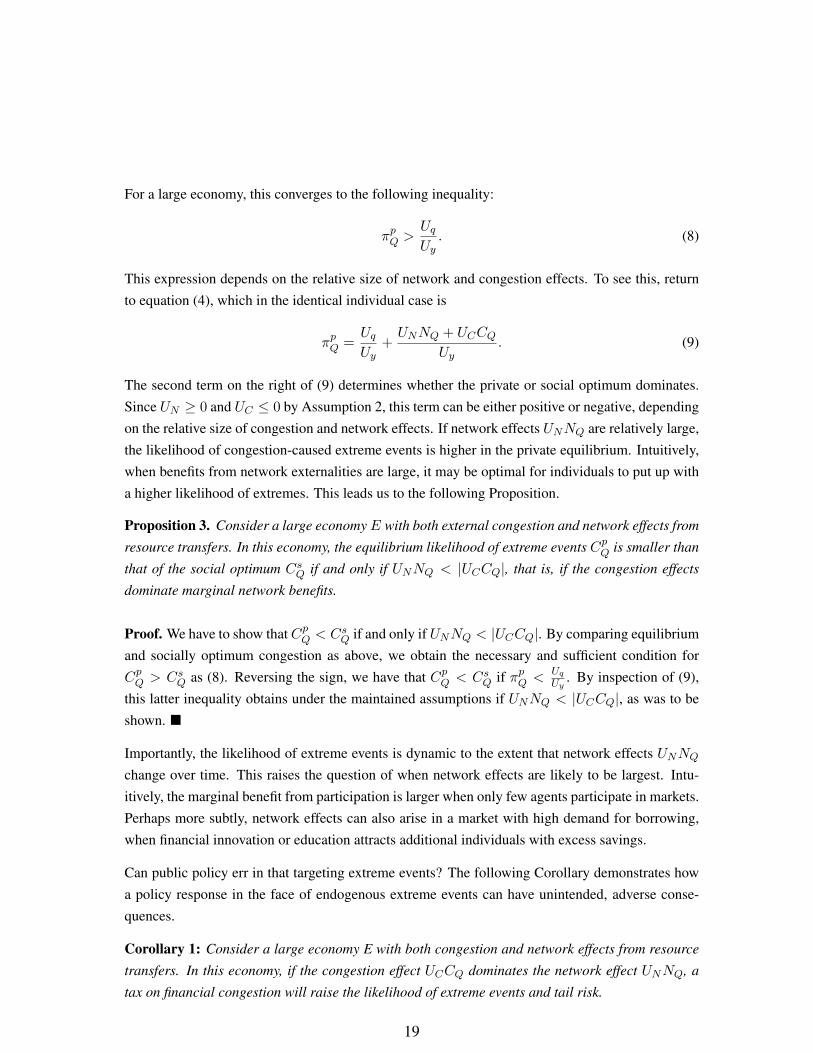
For a large economy, this converges to the following inequality:

πpQ >

Uq

Uy. (8)

This expression depends on the relative size of network and congestion effects. To see this, returnto equation (4), which in the identical individual case is

πpQ =

Uq

Uy+

UNNQ + UCCQ

Uy. (9)

The second term on the right of (9) determines whether the private or social optimum dominates.Since UN ≥ 0 and UC ≤ 0 by Assumption 2, this term can be either positive or negative, dependingon the relative size of congestion and network effects. If network effects UNNQ are relatively large,the likelihood of congestion-caused extreme events is higher in the private equilibrium. Intuitively,when benefits from network externalities are large, it may be optimal for individuals to put up witha higher likelihood of extremes. This leads us to the following Proposition.

Proposition 3. Consider a large economy E with both external congestion and network effects fromresource transfers. In this economy, the equilibrium likelihood of extreme events Cp

Q is smaller thanthat of the social optimum Cs

Q if and only if UNNQ < |UCCQ|, that is, if the congestion effectsdominate marginal network benefits.

Proof. We have to show that CpQ < Cs

Q if and only if UNNQ < |UCCQ|. By comparing equilibriumand socially optimum congestion as above, we obtain the necessary and sufficient condition forCpQ > Cs

Q as (8). Reversing the sign, we have that CpQ < Cs

Q if πpQ <

Uq

Uy. By inspection of (9),

this latter inequality obtains under the maintained assumptions if UNNQ < |UCCQ|, as was to beshown. �

Importantly, the likelihood of extreme events is dynamic to the extent that network effects UNNQ

change over time. This raises the question of when network effects are likely to be largest. Intu-itively, the marginal benefit from participation is larger when only few agents participate in markets.Perhaps more subtly, network effects can also arise in a market with high demand for borrowing,when financial innovation or education attracts additional individuals with excess savings.

Can public policy err in that targeting extreme events? The following Corollary demonstrates howa policy response in the face of endogenous extreme events can have unintended, adverse conse-quences.

Corollary 1: Consider a large economy E with both congestion and network effects from resourcetransfers. In this economy, if the congestion effect UCCQ dominates the network effect UNNQ, atax on financial congestion will raise the likelihood of extreme events and tail risk.

19

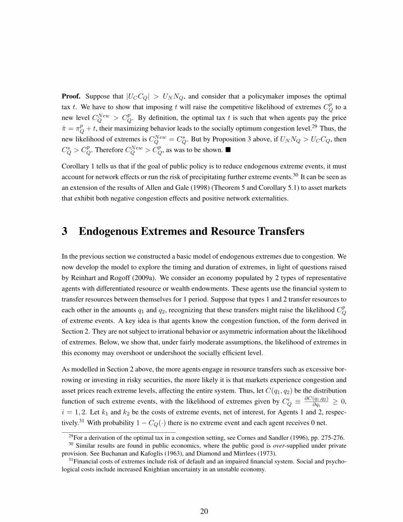
Proof. Suppose that |UCCQ| > UNNQ, and consider that a policymaker imposes the optimaltax t. We have to show that imposing t will raise the competitive likelihood of extremes Cp

Q to anew level CNew

Q > CpQ. By definition, the optimal tax t is such that when agents pay the price

π = πpQ + t, their maximizing behavior leads to the socially optimum congestion level.29 Thus, the

new likelihood of extremes is CNewQ = Cs

Q. But by Proposition 3 above, if UNNQ > UCCQ, thenCsQ > Cp

Q. Therefore CNewQ > Cp

Q, as was to be shown. �

Corollary 1 tells us that if the goal of public policy is to reduce endogenous extreme events, it mustaccount for network effects or run the risk of precipitating further extreme events.30 It can be seen asan extension of the results of Allen and Gale (1998) (Theorem 5 and Corollary 5.1) to asset marketsthat exhibit both negative congestion effects and positive network externalities.

3 Endogenous Extremes and Resource Transfers

In the previous section we constructed a basic model of endogenous extremes due to congestion. Wenow develop the model to explore the timing and duration of extremes, in light of questions raisedby Reinhart and Rogoff (2009a). We consider an economy populated by 2 types of representativeagents with differentiated resource or wealth endowments. These agents use the financial system totransfer resources between themselves for 1 period. Suppose that types 1 and 2 transfer resources toeach other in the amounts q1 and q2, recognizing that these transfers might raise the likelihood Cp

Q

of extreme events. A key idea is that agents know the congestion function, of the form derived inSection 2. They are not subject to irrational behavior or asymmetric information about the likelihoodof extremes. Below, we show that, under fairly moderate assumptions, the likelihood of extremes inthis economy may overshoot or undershoot the socially efficient level.

As modelled in Section 2 above, the more agents engage in resource transfers such as excessive bor-rowing or investing in risky securities, the more likely it is that markets experience congestion andasset prices reach extreme levels, affecting the entire system. Thus, let C(q1, q2) be the distributionfunction of such extreme events, with the likelihood of extremes given by Ci

Q ≡ ∂C(q1,q2)∂qi

≥ 0,i = 1, 2. Let k1 and k2 be the costs of extreme events, net of interest, for Agents 1 and 2, respec-tively.31 With probability 1− CQ(·) there is no extreme event and each agent receives 0 net.

29For a derivation of the optimal tax in a congestion setting, see Cornes and Sandler (1996), pp. 275-276.30 Similar results are found in public economics, where the public good is over-supplied under private

provision. See Buchanan and Kafoglis (1963), and Diamond and Mirrlees (1973).31Financial costs of extremes include risk of default and an impaired financial system. Social and psycho-

logical costs include increased Knightian uncertainty in an unstable economy.

20

For concreteness, the two main agents each conduct only one type of resource transfer–only sellingand buying. We call these agents sellers and buyers, respectively. The transfer of resources mayaffect other agents in the economy, including other buyers, sellers, banks and investors, domesticallyand internationally. We denote these other agents by O, for other. In the following analysis we usesubscripts 0, 1 and 2 to index variables pertaining to other, sellers and buyers, respectively.

We now develop this setting to incorporate time. Sellers and buyers are both in the market fortransferring resources. Effective supply of resources by sellers is q1 and demand for resources bybuyers is q2. The framework is a two-period economy, where the first period is t and the secondperiod is t + 1, in order to distinguish subscripts that refer to time from those that refer to agents.In the first period sellers and buyers interact and transfer resources. In the second period, sellersare repaid with interest q1,t · (1 + i), and buyers repay the resources, q2,t · (1 + i), where i is theprevailing interest rate. For simplicity, assume that agents receive all their wealth and make all theirrepayments in the second period.32 Thus, the seller’s and buyer’s wealth levels in the first periodcompletely derive from resource transfers: w1,t = −q1,t, and w2,t = q2,t, respectively. In the secondperiod t+ 1, the buyer and seller receive exogenous wealth endowments w1 and w2, respectively.

We focus on representative sellers and buyers with neoclassical utility functions u1 and u2, re-spectively, which depend on wealth: ui = ui(wi), where u′i(wi) > 0, i = 1, 2. To control forcontemporaneous costs, we consider utility to be net of current costs. Each agent knows there is apossibility of systemwide extreme events, captured by the probability CQ, whose functional formis common knowledge. There is no asymmetric information regarding the likelihood of extremes.33

As described in Section 2, the probability of future extreme events increases with the average levelof current resource transfers, Ct+1(·) = Ct+1(q1,t, q2,t), where Ci

Q,t+1 ≡ ∂Ct+1(·)∂qi,t

≥ 0, i = 1, 2.34

If an extreme event occurs in the future, agent i incurs a positive cost ki,t+1, i = 0, 1, 2. Our resultsdepend on properties of k, so we analyze two cases, finite k and potentially infinite k.

32This timing allows us to model the use of financial markets to transfer wealth over time.33Similar assumptions occur in many other economic contexts, such as price taking, competitive agents

in Arrow and Debreu (1954) and Debreu (1959), even though the demand of each agent will affect price tosome extent. Such myopic behavior can be found in other rational settings: investors with log utility decidetheir portfolios without reference to future investment opportunities, see Ingersoll (1987), chapter 11.

34 This summarizes the intuition that excessive resource transfers are destabilizing, without emphasizingthe particular channel of destabilization. Channels through which resource transfers lead to increased likeli-hood of extremes are explored by a number of authors, including Fisher (1933), Allen and Gale (2000), andKrishnamurthy (2010).

21

3.1 Large but Finite Costs k of Extreme Events

Suppose 0 < k1,t+1 < ∞ and consider the seller’s problem. Given an interest rate i, at period t

the seller decides how much resources to transfer this period by maximizing utility subject to thefollowing wealth constraint, which accounts for the possibility of costly extreme events:

w1,t+1 ≥ w1 + Ct+1(q1,t, q2,t)[q1,t · (1 + i)− k1,t+1] + [1− Ct+1(q1,t, q2,t)][q1,t · (1 + i)].

Given locally nonsatiated preferences, this constraint holds as an equality, which simplifies tow1,t+1 = w1 + q1,t · (1 + i) − Ct+1(q1,t, q2,t) · k1,t+1. Using β to denote the discount factor,the seller’s problem is:

maxq1 u1(w1,t) + βu1(w1,t+1), s.t.

w1,t = −q1,t

w1,t+1 = w1 + q1,t · (1 + i)− Ct+1(q1,t, q2,t) · k1,t+1.

After substituting the constraints into the utility arguments, first order conditions for an interiorsolution are −u′1(w1,t)+βu′1(w1,t+1)[(1+ i)− ∂Ct+1(q1,t,q2,t)

∂q1,t·k1,t+1] = 0, which can be rewritten

asC1Q,t+1 ≡

∂Ct+1(q1,t, q2,t)

∂q1,t= − u′1(w1,t)

βu′1(w1,t+1) · k1,t+1+

1 + i

k1,t+1. (10)

Equation (10) says that optimally the probability of extremes is related to the marginal rate ofsubstitution for transferring resources between periods t and t + 1, discounted by expected costs.Since the first term of the right hand side of (10) depends on q1,t via the budget constraint, it followsthat extreme probabilities respond to variables affecting the level of resource transfers.

Similarly, the buyer’s problem is

maxq2 u2(w2,t) + βu2(w2,t+1), s.t.

w2,t = q2,t

w2,t+1 = w2 − q2,t · (1 + i)− Ct+1(q1,t, q2,t) · k2,t+1,

which yields first order conditions that can be rewritten as

C2Q,t+1 ≡

∂Ct+1(q1,t, q2,t)

∂q2,t=

u′2(w2,t)

βu′2(w2,t+1) · k2,t+1− 1 + i

k2,t+1. (11)

As in equation (10), the above expression implies that the future probability of extremes is poten-tially dynamic, and depends on the current level of resource transfers.

22

Equilibrium: In equilibrium, the effective demand and effective supply of resource transfers willbe equal, q1 = q2 ≡ q. For illustrative purposes, consider a symmetric equilibrium where buyersand sellers have identical utility functions and costs, u1 = u2 = u, and k1 = k2 = k. Nowequate optimality conditions for the seller and buyer in (10) and (11): − u′(w1,t)

βu′(w1,t+1)·kt+1+ 1+i

kt+1=

u′(w2,t)βu′(w2,t+1)·kt+1

− 1+ikt+1

. This implies

1 + i =1

2β

[u′(w1,t)

u′(w1,t+1)+

u′(w2,t)

u′(w2,t+1)

].

Substituting this expression in equation (11) and simplifying, we obtain that in equilibrium, extremeprobabilities CQ,t+1 satisfy

CQ,t+1 ≡∂Ct+1

∂qt=

1

2βkt+1

[u′(w2,t)

u′(w2,t+1)− u′(w1,t)

u′(w1,t+1)

](12)

Equation (12) constitutes the signature of endogenous extremes. Somewhat surprisingly, the respon-siveness of extreme probability to resource transfers is proportional to the differential in marginalrates of substitution for agents in the corresponding market. When there is a big difference inmarginal rates of substitutions between borrowers and lenders, the susceptibility to extreme eventsis higher. As before, the extreme probability is dynamic: it depends directly on the expected costsof extremes, and indirectly (with indeterminate sign) on the equilibrium level of resource transfersvia the budget constraint. If extremes were truly exogenous, there would be no statistical relationbetween extreme probability and q, and ∂C(qt+1)

∂qt= 0. Thus, the distance of the right side of (12)

from zero gives a sense of the error from assuming extremes are exogenous, when they are in realityendogenous.

Importantly, there are 2 main countervailing effects. First is the kt+1 cost term in the denominator:the larger it is, the less likelihood of congestion since it negatively affects utility. Second is the dif-ference in marginal rates of substitution u′(w2,t)

u′(w2,t+1)− u′(w1,t)

u′(w1,t+1): the larger this is, the more attractive

for individuals to transfer. In addition, there is a latent effect of resource transfers qt, which operatethrough the budget constraint.

We summarize the results from (12) in the following Proposition.

Proposition 4. In an economy with symmetric preferences and nonzero social costs of extremes,the likelihood of extremes CQ is potentially dynamic. CQ depends indeterminately on equilibriumresource transfers; decreases with expected costs of extreme events kt+1; and increases with thedivergence between agents’ marginal rates of substitution.

Proof: By examination of (12). �

23

An immediate result of the above proposition is that the likelihood of extremes becomes arbitrarilylow when marginal rates of substitution are equated. This gives us information about timing andexpected duration of extreme events, as summarized in the following Corollary.

Corollary 2. In an economy with symmetric preferences and nonzero social costs of extremes,extreme episodes will persist until the marginal rates of substitution are equated, or if expectedcosts of extremes rise high enough .

Proof: By examination of (12). �

Social Optimum. We now consider optimality issues. To see that the likelihood of extremes isinefficient in competitive equilibrium, suppose the seller considers the effect of her selling on otheragents O, and therefore internalizes costs k0,t+1. Her problem is similar to that preceding equation(10), except that the second budget constraint becomes

w1,t+1 = w1 + q1,t · (1 + i)− Ct+1(q1,t, q2,t) · (k0,t+1 + k1,t+1).

Solving the first order conditions and rewriting as before, we obtain the counterpart of equation (10)for a socially optimal level of extremes:

∂Ct+1(q1,t, q2,t)

∂q1,t= − u′1(w1,t)

βu′1(w1,t+1) · (k0,t+1 + k1,t+1)+

1 + i

k0,t+1 + k1,t+1. (13)

The quantities in equations (10) and (13) will differ in general. Thus, when the resource seller takesinto account the future costs of other agents, optimizing behavior delivers a different likelihood ofextremes. It is in this sense that competitive markets may lead to endogenous, inefficient proba-bility of crashes.35 We are not just saying there is a link between excessive resource transfers andextremes. Instead, we are showing that even without asymmetric information or irrationality, ex-treme events may arise as an equilibrium phenomenon, to the extent that ∂Ct+1(q1,t,q2,t)

∂q1,t= 0. This

phenomenon occurs due to the failure of both resource sellers and buyers to internalize an importantexternality, the expected costs from congestion, which affect the probability of systemwide, futurefinancial extremes.

Importantly, as in Section 2, we cannot determine a priori whether the likelihood of extremes islarger in the competitive equilibrium or the social optimum. We summarize our results from equa-tions (10), and (13) in the following Proposition:

35Optimality will not necessarily entail complete elimination of extreme events. Rather, the extreme prob-ability is adjusted to the point where marginal benefit to sellers of an additional unit of the externality-generating activity, u′

1(q), equals marginal cost to other agents, −u′0(q).

24

Proposition 5. In an economy with symmetric preferences and nonzero social costs of extremes, theequilibrium level of extreme probability is in general not socially optimal. Moreover, the likelihoodof extremes may be smaller or larger in competitive markets.

Proof: By comparison of (10) and (13). �

3.2 Potentially Infinite Costs k of Extreme Events

Recent financial events have potentially catastrophic consequences that are difficult to quantify exante. These events include the costs of the Japan earthquake and nuclear meltdown in January 2011,the US debt default scare in early August 2011, the Greece debt crises of April 2010 and June 2011,and the financial crisis inception in September 2008. In order to capture such events, we considerthe possibility of infinite expected costs of extremes for each type of agent. Specifically, supposek1,t+1 = ∞ and consider the seller’s problem as in section 3.1 above. Once again, her maximizationprogram is

maxq1 u1(w1,t) + βu1(w1,t+1), s.t.

w1,t = −q1,t

w1,t+1 = w1 + q1,t · (1 + i)− Ct+1(q1,t, q2,t) · k1,t+1.

However, now the agent’s program involves optimizing over a quantity of infinite magnitude, whichoften leads to corner solutions. To see this, substitute the constraints into the maximand, whichbecomes

u1(−q1,t) + βu1 (w1 + q1,t · (1 + i)− Ct+1(q1,t, q2,t) · k1,t+1) (14)

Since the second term involves minus infinity, the only solution for a risk-averse individual is to setq1,t = 0, so that Ct+1(·) is as close to zero as possible. A similar logic applies to the seller. Weremove the subscript on k for simplicity and summarize this result in the following Proposition.

Proposition 6. Consider an economy where agents transfer resources, and in which there is com-mon knowledge about the likelihood of extreme events, captured by the function C(Q). If the ex-pected cost of extreme events k is infinite, then risk-averse agents will not transfer resources.

Proof. The agent’s problem involves choosing transfers q1 to maximize (14). If k = ∞ thenthe second term becomes −∞. This implies unbounded negative utility for a risk-averter, un-less Ct+1(·) = 0. The agent will therefore set q1 = 0, which according to Assumption 3 yieldsCt+1(·) = 0. q1 = 0 corresponds to non-transferral of resources. �

25

According to Proposition 6, if agents face extreme events with arbitrarily large consequences, theonly way they will trade is if they are risk neutral or risk-loving.36

3.3 Summary and Implications

The preceding results have implications for regulatory policy and risk management. Proposition4 cautions risk managers against the assumption that exposure to extreme events is constant overtime. Further, Proposition 4 suggests possible warning signals for regulators and risk managers–lowexpected costs and a large gap between agents’ desires to transfer resources over time.37 Proposi-tion 5 and Corollary 1 suggest, in principle, a role for regulators and central banks to interveneand prevent excessive financial extremes. However, these latter results also caution regulators thattheir intervention might inadvertently increase the likelihood of extremes, in a manner that has notpreviously been examined.38

More tentatively, the results may also have relevance for current financial issues in the US and Eurozone. Proposition 4 suggests that the increased likelihood of extremes in today’s markets have beenprecipitated by low expected costs previously (e.g. on the part of Greek debtors) and by a large gapbetween the marginal rates of substitution for borrowers and lenders of capital. After expected costsrise and marginal rates of substitution converge, then the elevated extremes will begin to play out.

4 Conclusions

Our paper develops a simple approach to endogenous extreme events. We suggest that the prob-ability of extremes may vary systematically over time, and be explained on the basis of financialcongestion and network effects. Moreover, we distinguish exogenous from endogenous extremes,the latter of which can be understood in a public good framework. This distinction has immedi-ate policy implications: for truly exogenous extremes, we must focus on ex post protection, whilefor endogenous extremes, we can in principle use economic incentives to entice agents to reduceextremes themselves. We have three main contributions. First, we develop the ’signature’ of en-

36If markets are thin, then even risk-loving agents will be unable to transfer resources.37More generally, Proposition 4 predicts that developments to enhance resource transfers will affect the

likelihood of extremes. These developments include may financial innovation and loose interest rates.38Theoretically, regulators could tax ’excessive’ transfers. However, this requires extensive monitoring of

investor positions. A more realistic approach involves combining regulation with enhanced education aboutcosts of extreme events, and the role of individuals and institutions in precipitating these costs. This approachis similar to recent education about other externalities such as effects of drunk driving, cigarette smoking,and human impact on the natural environment.

26

dogenous extremes, and provide insight on their incidence: According to Proposition 4, economiesare more susceptible to extremes if expected costs are low and there is a large discrepancy betweenmarginal rates of substitutions for resource borrowers and lenders. Second, extreme episodes lastuntil marginal rates of substitution converge, or expected costs rise. Third and perhaps most in-teresting, our approach (Corollary 1) suggests limits on the role for central bank and regulatoryintervention. In tackling issues related to economic instability, regulators can ameliorate the likeli-hood of extremes, but only if they account for countervailing network effects.

While our paper describes a method for understanding patterns in the likelihood of extremes, it doesnot aim to predict all possible extreme events. The aim is to show that, far from being random, theprobability of endogenous extremes may have similar patterns. We accomplished this aim using abroad congestion-network approach, which allows us to relate the likelihood of extremes to eco-nomic variables: resource transfers, expected costs and marginal rates of substitution. Our papermay be seen as a step towards incorporating dynamic, endogenous, extremes into standard economicanalysis. Acknowledgement of endogenous extremes may also be helpful for risk management.Important extensions include estimating financial congestion, identifying dynamic extremes in par-ticular markets, and exploring various channels of endogenous extremes encountered in practice.Such refinements present an exciting task for future research.

27

ReferencesAbreu, D., Brunnermeier, M., 2003. Bubbles and crashes. Econometrica 71 (1), 173–204.

Acharya, A., Cooley, T., Richardson, M., Walter, I., 2010a. Manufacturing tail risk: A perspectiveon the financial crisis of 2007-2008. Foundations and Trends in Finance 4 (4), 247–325.

Acharya, V., Brownlees, C., Engle, R., Farazmand, F., Richardson, M., 2010b. Measuring systemicrisk. In: Acharya, V., Cooley, T., Richardson, M., Walter, I. (Eds.), Regulating Wall Street: TheDodd-Frank Act and the New Architecture of Global Finance. John Wiley and Sons, New York,pp. 87–120.

Acharya, V., Pedersen, L., Philippon, T., Richardson, M., 2010c. A tax on systemic risk. In:Acharya, V., Cooley, T., Richardson, M., Walter, I. (Eds.), Regulating Wall Street: The Dodd-Frank Act and the New Architecture of Global Finance. John Wiley and Sons, New York, pp.121–142.

Adrian, T., Brunnermeier, M., 2010. Covar: A systemic risk contribution measure. Tech. rep.,Princeton University.

Agarwal, S., Driscoll, J., Gabaix, X., Laibson, D., 2007. The age of reason: Financial decisions overthe lifecycle. Tech. rep., Harvard.

Aitken, M., Comerton-Forde, C., 2003. How should liquidity be measured? Pacific-Basin FinanceJournal 11, 45–59.

Allen, F., Carletti, E., Krahnen, J., Tyrell, M., 2011. Liquidity and Crises. Oxford University Press,New York.

Allen, F., Gale, D., 1998. Optimal financial crises. Journal of Finance LIII (4), 1245–1284.

Allen, F., Gale, D., 2000. Comparing Financial Systems. MIT Press, MA.

Allen, F., Gale, D., 2007. Understanding Financial Crises. Clarendon Lectures in Finance. OxfordUniversity Press.

Amihud, Y., 2002. Illiquidity and stock returns: Cross-section and time-series effects. Journal ofFinancial Markets 5, 31–56.

Arrow, K., Debreu, G., 1954. Existence of an equilibrium for a competitive economy. Econometrica22, 265–290.

Baker, M., Wurgler, J., 2007. Investor sentiment in the stock market. Journal of Economic Perspec-tives 21 (2), 129 – 151.

Banerjee, A., 1992. A simple model of herd behavior. Quarterly Journal of Economics 107 (3),797–817.

Bansal, R., Shaliastovich, I., 2010. Confidence risk and asset prices. American Economic ReviewXXX (XXX), 1–5.

28

Barber, B., Odean, T., 2000a. Too many cooks spoil the profits: The performance of investmentclubs. Financial Analyst Journal January/February, 17–25.

Barber, B., Odean, T., 2000b. Trading is hazardous to your wealth: The common stock investmentperformance of individual investors. Journal of Finance LV (2), 773–806.

Barro, R., 2006. Rare disasters and asset markets in the twentieth century. Quarterly Journal ofEconomics 121 (3), 823–866.

Baumol, W., Oates, W., 1988. The Theory of Environmental Policy, Second Edition. Prentice Hall,New Jersey.

Bazerman, M., Watkins, D., 2004. Predictable Surprises. Harvard Business School Press.

Below, R., Guha-Sapir, D., Hoyois, P., Scheuren, J.-M., 2007. Annual Disaster Statistical Review:Numbers and Trends, 2006. Center for Research on the Epidemiology of Disasters (CRED).

Benartzi, S., Thaler, R., 1995. Myopic loss aversion and the equity premium puzzle. QuarterlyJournal of Economics 110 (1), 73–92.

Benhabib, J., Farmer, R., 1999. Indeterminacy and sunspots in macroeconomics. Handbook ofMacroeconomics 1A, 387–448.

Bernanke, B., Gertler, M., 1989. Agency costs, net worth, and business fluctuations. AmericanEconomic Review 79 (1), 14–31.

Bernanke, B., Gertler, M., 2001. Should central banks respond to movements in asset prices? Amer-ican Economic Review 91 (2), 253–257.

Bianchi, J., 2010. Credit externalities: Macroeconomic effects and policy implications. AmericanEconomic Review 100 (2), 398–402.

Bianchi, J., 2011. Overborrowing and systemic externalities in the business cycle. American Eco-nomic Review, forthcoming.

Bianchi, J., Mendoza, E., 2011. Overborrowing, financial crises and macroprudential policy. Tech.rep., University of Maryland.

Bikhchandani, S., Hirschliefer, D., Welch, I., 1992. A theory of fads, fashion, custom, and culturalchange as informational cascades. Journal of Political Economy 100, 992–1026.

Blanchard, O., 1979. Speculative bubbles, crashes and rational expectations. Economics Letters 3,387–389.

Blanchard, O., Kiyotaki, N., 1987. Monopolistic competition and the effects of aggregate demand.American Economic Review 77 (4), 647–666.

Bollerslev, T., Todorov, V., 2011. Tails, fears, and risk premia. Journal of Finance, forthcoming.

29

Brunnermeier, M., Pedersen, L., 2009. Market liquidity and funding liquidity. Review of FinancialStudies 22 (6), 2201–2238.

Brunnermeier, M., Sannikov, Y., 2011. A macroeconomic model with a financial sector. Tech. rep.,Princeton University.

Buchanan, J., Kafoglis, M., 1963. A note on public goods supply. American Economic Review 53,403–414.

Caballero, R., Krishnamurthy, A., 2008. Collective risk management in a flight to quality episode.Journal of Finance LXIII (5), 2195–2230.

Camerer, C., 1989. Bubbles and fads in asset prices. Journal of Economic Surveys 3 (1), 3–41.

Chollete, L., Heinen, A., Valdesogo, A., 2009. Modeling international financial returns with a mul-tivariate regime-switching copula. Journal of Financial Econometrics 7 (4), 437–480.

Cooper, R., 1999. Coordination Games: Complementarities and Macroeconomics. CambridgePress, New York.

Cornes, R., Sandler, T., 1996. The Theory of Externalities, Public Goods and Club Goods, SecondEdition. Cambridge University Press, New York.

Danielsson, J., Shin, H., 2003. Endogenous risk. Tech. rep., LSE.

Danielsson, J., Zigrand, J., 2008. Equilibrium asset pricing with systemic risk. Economic Theory35, 293–319.

Debreu, G., 1959. Theory of Value: An Axiomatic Analysis of Economic Equilibrium. Yale Uni-versity Press.

Diamond, P., Mirrlees, J., 1973. Aggregate production with consumption externalities. QuarterlyJournal of Economics 87, 1–24.

Duffie, D., 2010. Asset price dynamics with slow-moving capital. Journal of Finance 65, 1238–1268.

Easley, D., Kleinberg, J., 2010. Networks, Crowds and Markets: Reasoning about a Highly Con-nected World. Cambridge University Press, New York.

Embrechts, P., McNeil, A., Straumann, D., 2002. Correlation and dependence in risk managament:Properties and pitfalls. In: Dempster, M. (Ed.), Risk Management: Value at Risk and Beyond.Cambridge University Press, Cambridge, UK, pp. 176–223.

Fama, E., 1965. The behavior of stock market prices. Journal of Business 38, 34–105.

Fisher, I., 1933. The debt-deflation theory of great depressions. Econometrica 1 (4), 337–357.

Fostel, A., Geanakoplos, J., 2008. Leverage cycles and the anxious economy. American EconomicReview 98 (4), 1211–1244.

30

Friedman, B., Laibson, D., 1989. Economic implications of extraordinary movements in stockprices. Brookings Papers on Economic Activity, 137–172.

Froot, K., Scharfstein, D., Stein, J., 1992. Herd on the street: Informational inefficiencies in a marketwith short-term speculation. Journal of Finance 47 (4), 1461–1484.

Gabaix, X., 2008. Variable rare disasters: A tractable theory of ten puzzles in macro-finance. Amer-ican Economic Review: Papers and Proceedings 98 (2), 64–67.

Gabaix, X., 2010a. The granular origins of aggregate fluctuations. Econometrica, forthcoming.

Gabaix, X., 2010b. Variable rare disasters: An exactly solved framework for ten puzzles in macro-finance. Tech. rep., New York University.

Gabaix, X., Gopikrishnan, P., Plerou, V., Stanley, H., 2006. Institutional investors and stock marketvolatility. Quarterly Journal of Economics 121 (2), 461–504.

Goetzmann, W., Rouwenhorst, K., 2005. The Origins of Value: The Financial Innovations thatCreated Modern Capital Markets. Oxford University Press, New York.

Goyenko, R., Holden, C., Trzcinka, C., 2009. Do liquidity measures measure liquidity? Journal ofFinancial Economics 92, 153–181.

Grossman, S., 1988. An analysis of the implications for stock and futures price volatility of programtrading and dynamic hedging strategies. Journal of Business 61 (3), 275–298.

Harris, L., 2003. Trading and Exchanges. Market Microstructure for Practitioners. Oxford Univer-sity Press.

Harrison, S., 2001. Indeterminacy in a model with sector-specific externalities. Journal of EconomicDynamics and Control 25 (5), 747–764.

Hartmann, P., Straetmans, S., de Vries, C., 2003. A global perspective on extreme currency linkages.In: Hunter, W. C., Kaufman, G. G., Pomerleano, M. (Eds.), Asset Price Bubbles: Implicationsfor Monetary, Regulatory and International Policies. MIT Press, Cambridge, pp. 361–382.

Hartmann, P., Straetmans, S., de Vries, C., 2004. Asset market linkages in crisis periods. The Re-view of Economics and Statistics 86 (1), 313–326.

Hong, H., Scheinkman, J., Xiong, W., 2008. Advisors and asset prices: A model of the origins ofbubbles. Journal of Financial Economics 89, 268–287.

Ibragimov, R., Jaffee, D., Walden, J., 2009. Non-diversification traps in catastrophe insurance mar-kets. Review of Financial Studies 22 (3), 959–993.

Ibragimov, R., Jaffee, D., Walden, J., 2011. Diversification disasters. Journal of Financial Eco-nomics 99, 333–348.

Ibragimov, R., Walden, J., 2007. The limits of diversification when losses may be large. Journal ofBanking and Finance 31, 2551–2569.

31

Ingersoll, J., 1987. Theory of Financial Decision Making. Rowman and Littlefield Publishers, NewYork.

Jansen, D., de Vries, C., 1991. On the frequency of large stock returns: Putting booms and bustsinto perspective. The Review of Economics and Statistics 73 (1), 18–24.

Katz, M., Shapiro, C., 1985. Network externalities, competition and compatibility. American Eco-nomic Review 75 (3), 424–440.

Keynes, J., 1936. The General Theory of Employment, Interest and Money. Harcourt, Brace, andCompany, New York.

Kiyotaki, N., Moore, J., 1997. Credit cycles. Journal of Political Economy 105 (2), 211–248.

Krishnamurthy, A., 2010. Amplification mechanisms in liquidity crises. American EconomicJournal-Macroeconomics 2 (3), 1–30.

Liu, J., Longstaff, F., Pan, J., 2003. Dynamic asset allocation with event risk. Journal of FinanceLVIII (1), 231–259.

Liu, J., Longstaff, F., Pan, J., 2005. An equilibrium model of rare-event premia and its implicationfor option smirks. Review of Financial Studies 18 (1), 231–259.

Longin, F., Solnik, B., 2001. Extreme correlation of international equity markets. Journal of Finance56 (2), 649–76.

Mandelbrot, B., 1963. The variation of certain speculative prices. Journal of Business 36, 394–419.

Mas-Colell, A., Whinston, M., Green, J., 1995. Microeconomic Theory. Oxford Press.

Minsky, H., 1982. Can it Happen Again? Essays on Instability and Finance. M. E. Sharpe, NewYork.

Montier, J., 2002. Behavioural Finance: Insights into Irrational Minds and Markets. John Wiley andSons, Chichester, England.

Morris, S., Shin, H., 1998. Unique equilibrium in a model of self-fulfilling currency attacks. Amer-ican Economic Review 88 (3), 587–597.

Morris, S., Shin, H., 2011. Contagious adverse selection. American Economic Journal: Macroeco-nomics forthcoming.

Myles, G., 1995. Public Economics. Cambridge University Press, New York.

Odean, T., 1999. Do investors trade too much? American Economic Review 89, 1279–1298.

Pedersen, L., 2007. Slow-moving capital. American Economic Review 97 (2), 215–220.

Pedersen, L., 2009. When everyone runs for the exit. International Journal of Central Banking 5 (4),177–199.

32

Phelps, E., 2007. Macroeconomics for a modern economy. American Economic Review 97 (3),543–561.

Poon, S., Rockinger, M., Tawn, J., 2004. Extreme value dependence in financial markets: Diagnos-tics, models, and financial implications. Review of Financial Studies 17 (2), 581–610.

Rajan, R., 2010. Fault Lines: How Hidden Fractures Still Threaten the World Economy. PrincetonUniversity Press, New Jersey.

Reinhart, C., Rogoff, K., 2009a. The aftermath of financial crises. American Economic Review99 (2), 466–472.

Reinhart, C., Rogoff, K., 2009b. This Time is Different: 800 Years of Financial Folly. PrincetonPress.

Rostek, M., Weretka, M., 2010. Dynamic thin markets. Tech. rep., University of Wisconsin-Madison.

Rostek, M., Weretka, M., 2011. Price inference in small markets. Econometrica, forthcoming.

Sadka, R., Koracjczyk, R., 2008. Pricing the comonality across alternative measures of liquidity.Journal of Financial Economics 87, 45–72.

Shapiro, C., Varian, H., 1998. Information Rules: A Strategic Guide to the Network Economy.Harvard Business Press, MA.

Shin, H., 2009. Securitisation and system stability. Economic Journal 119, 309–322.

Shin, H., 2010. Risk and Liquidity. Oxford University Press, New York.

Shleifer, A., Vishny, R., 1997. The limits of arbitrage. Journal of Finance LII (I), 35–55.

Sornette, D., 2004. Why Stock Markets Crash: Critical Events in Complex Financial Systems.Princeton University Press.

Stein, J., 2009. Sophisticated investors and market efficiency. Journal of Finance LXIV (4), 1517–1548.

Stern, N., 2007. The Economics of Climate Change: The Stern Review. Cambridge Press.

Susmel, R., 2001. Extreme observations and diversification in latin american emerging equity mar-kets. Journal of International Money and Finance 20, 971–986.

Varian, H., 1992. Microeconomic Analysis. Norton and Company, New York.

Veldkamp, L., 2011. Information Choice in Macroeconomics and Finance. Princeton Press.

Veldkamp, L., Van Nieuwerburgh, S., 2010. Information acquisition and under-diversification. Re-view of Economic Studies 77 (2), 779–805.

33

Vives, X., 2008. Information and Learning in Markets: The Impact of Market Microstructure.Princeton Press.

Wachter, J., 2011. Can time-varying risk of rare disasters explain aggregate stock market volatility?Tech. rep., Wharton.

Wagner, W., 2011. Systemic liquidation risk and the diversity-diversification tradeoff. Journal ofFinance, forthcoming.

Weitzman, M., 2007. Subjective expectations and asset return puzzles. American Economic Review97 (4), 1102–1130.

34

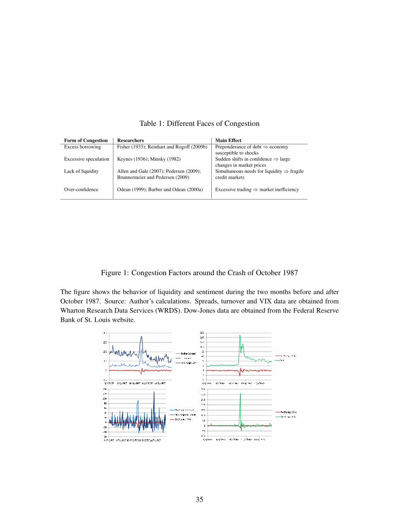
Table 1: Different Faces of Congestion

Form of Congestion Researchers Main EffectExcess borrowing Fisher (1933); Reinhart and Rogoff (2009b) Preponderance of debt ⇒ economy

susceptible to shocksExcessive speculation Keynes (1936); Minsky (1982) Sudden shifts in confidence ⇒ large

changes in market pricesLack of liquidity Allen and Gale (2007); Pedersen (2009); Simultaneous needs for liquidity ⇒ fragile

Brunnermeier and Pedersen (2009) credit markets

Over-confidence Odean (1999); Barber and Odean (2000a) Excessive trading ⇒ market inefficiency

Figure 1: Congestion Factors around the Crash of October 1987

The figure shows the behavior of liquidity and sentiment during the two months before and afterOctober 1987. Source: Author’s calculations. Spreads, turnover and VIX data are obtained fromWharton Research Data Services (WRDS). Dow-Jones data are obtained from the Federal ReserveBank of St. Louis website.

-50050100150200

8/3/1987 9/3/1987 10/3/1987 11/3/1987 12/3/1987Dollar SpreadTurnover% Change DJIA

-40-20020406080100120140160

8/3/1987 9/3/1987 10/3/1987 11/3/1987 12/3/1987% Change DJIAVIX

-60-40-20020406080100120140

8/3/1987 9/3/1987 10/3/1987 11/3/198712/3/1987% Change Spread% Change Turnover% Change DJIA

-100-50050100150200250300350

8/3/1987 9/3/1987 10/3/1987 11/3/1987 12/3/1987% Change DJIA% Change VIX

35

Figure 2: Congestion around the LTCM crisis of August 1998

The figure shows the behavior of liquidity and sentiment during the two months before and afterAugust 1998. Source: Author’s calculations. Spreads, turnover and VIX data are obtained fromWharton Research Data Services (WRDS). Dow-Jones data are obtained from the Federal ReserveBank of St. Louis website.

-20020406080100120140160180

6/1/1998 7/1/1998 8/1/1998 9/1/1998 10/1/1998Dollar SpreadTurnover% Change DJIA

-100102030405060

6/1/1998 7/1/1998 8/1/1998 9/1/1998 10/1/1998% Change DJIAVIX

-100-50050100150200

6/1/1998 7/1/1998 8/1/1998 9/1/1998 10/1/1998% Change Spread% Change Turnover% Change DJIA -20-15-10-505

1015202530

6/1/1998 7/1/1998 8/1/1998 9/1/1998 10/1/1998% Change DJIA% Change Vix

Figure 3: Congestion around the Lehman Brothers Bankruptcy of September 2008

The figure shows the behavior of liquidity and sentiment during the two months before and afterSeptember 2008. Source: Author’s calculations. Spreads, turnover and VIX data are obtained fromWharton Research Data Services (WRDS). Dow-Jones data are obtained from the Federal ReserveBank of St. Louis website.

-20020406080100

7/1/2008 9/1/2008 11/1/2008% Change DJIAVIX

-1000100200300400500600700800900

7/1/2008 9/1/2008 11/1/2008Dollar SpreadTurnover% Change DJIA

-100-50050100150200250300% Change Spread% Change Turnover% Change DJIA

-40-30-20-10010203040

7/1/2008 9/1/2008 11/1/2008% Change DJIA% Change VIX

36

Figure 4: Congestion around the Flash Crash of May 2010

The figure shows the behavior of liquidity and sentiment during the two months before and afterthe Flash Crash of May 2010. Source: Author’s calculations. Spreads, turnover and VIX data areobtained from Wharton Research Data Services (WRDS). Dow-Jones data are obtained from theFederal Reserve Bank of St. Louis website.

-1000100200300400500600700

3/1/2010 5/1/2010 7/1/2010Dollar SpreadTurnover% Change DJIA

-100-50050100150200

3/1/2010 5/1/2010 7/1/2010% Change Spread% Change Turnover% Change DJIA

-1001020304050

3/1/2010 5/1/2010 7/1/2010% Change DJIAVIX

-40-30-20-10010203040

3/1/2010 5/1/2010 7/1/2010% Change DJIA% Change VIX

37

Table 2: Rank Correlations for the Dow Jones, Liquidity and VIX

The table presents the Spearman (rank) correlations of the liquidity and confidence measures withthe Dow Jones Industrial Average. APLIQ denotes the market average of the Amihud (2002) liq-uidity measure. SPREAD and TURNOVER denote the average dollar bid-ask spread and turnover,respectively. VIX is the implied volatility of an at-the-money 30-day option, which reflects investorconfidence. All variables are in percentage changes relative to the previous trading day. The timeperiod for each extreme event comprises the four months surrounding the month of the event: forthe October 1987 crash, the sample period is August 1, 1987 to December 31, 1987. For the August1998 LTCM event, the sample period is June 1, 1998 to October 31, 1998. For the September 2008episode around the Lehman Brothers Bankruptcy, the sample period is July 1, 2008 to November30, 2008. And for the May 2010 flash crash the period is March 1, 2010 to July 31, 2010. P-valuesare in parentheses.

Panel A: Correlations around October 1987DJIA ALIQ SPREAD TURNOVER VIX

ALIQ -0.133 1.000(0.176)

SPREAD -0.037 -0.155 1.000(0.704) (0.112)

TURNOVER 0.143 -0.240 0.716 1.000(0.143) (0.013) (<.0001)

VIX -0.659 0.123 0.210 0.080 1.000(<.0001) (0.210) (0.031) (0.416)

Panel B: Correlations around August 1998DJIA ALIQ SPREAD TURNOVER VIX

ALIQ 0.108 1.000(0.268)

SPREAD -0.126 -0.145 1.000(0.199) (0.139)

TURNOVER 0.125 -0.215 0.197 1.000(0.203) (0.027) (0.043)

VIX -0.837 -0.135 0.229 -0.032 1.000(<.0001) (0.169) (0.018) (0.742)

Panel C: Correlations around September 2008DJIA ALIQ SPREAD TURNOVER VIX

ALIQ -0.004 1.000(0.966)

SPREAD -0.035 0.118 1.000(0.720) (0.228)

TURNOVER 0.155 -0.139 0.525 1.000(0.113) (0.156) (<.0001)

VIX -0.866 -0.015 0.088 -0.032 1.000(<.0001) (0.881) (0.369) (0.748)

Panel D: Correlations around the May 2010 Flash CrashDJIA ALIQ SPREAD TURNOVER VIX

ALIQ -0.060 1.000(0.536)

SPREAD -0.152 0.169 1.000(0.117) (0.081)

TURNOVER -0.201 0.071 0.560 1.000(0.038) (0.467) (<.0001)

VIX -0.802 -0.004 0.210 0.275 1.000(<.0001) (0.967) (0.030) (0.004)

38

Table 3: Snapshot of Extreme Events in Financial Markets

Event Context Peak Trough % changePanel A: US CrashesOctober 28, 1929 Smoot-Hawley Tariff debate 301.22 260.64 −13.47%October 19, 1987 Algorithmic Trading 2246.74 1738.74 −22.61%August 31, 1998 LTCM, Russian Default 8051.68 7539.06 −6.37%September 17, 2001 9/11 9605.51 8920.70 −7.13%September 29, 2008 Lehman Brothers bankruptcy 11143.13 10365,45 −6.98%October 15, 2008 Emergency Econ. Stability Act 9310.99 8577.91 −7.87%May 6, 2010 Flash Crash 10868.12 10520.32 −3.20%August 8, 2011 US Debt Downgrade 11444.61 10809.85 −5.55%

Panel B: Hong Kong CrashesOctober 19-26, 1987 US spillover 3362.4 2241.7 −33.3%February 4 - March 3, 1994 Bubble 12157.6 9802 −19.4%October 17-28, 1997 Bubble 13601 9059.9 −33.4%

Source for Panel A: author calculations, based on data from the Federal Reserve Bank of St. Louis.Source for Panel B: Sornette (2004). US data are for the Dow-Jones Industrial Average. Hong Kongdata are for the Hang Seng Index.

Table 4: Two Examples of Endogenous Probabilities

Effects felt in one Spillover effectsmarket or transaction in many markets

Asymmetric Information Moral Hazard

Symmetric or AsymmetricInformation Endogenous Extremes

Table 5: Excessive Resource Transfers and Extreme Events

Form of Resource Transfer AuthorOver-borrowing, leverage Fisher (1933); Minsky (1982)Excessive credit creation Allen and Gale (2000)

Large sales due to confidence shifts Reinhart and Rogoff (2009b); Keynes (1936)Increased Trading Montier (2002); Gabaix et al. (2006)

Fire-sale asset liquidation Allen and Gale (2007)

39

Table 6: Summary of Results

Result Explanation

Proposition 1 If only congestion effects are present, competitive markets yield higher CQ(·)

Proposition 2 If both congestion and network effects, equilibrium congestion inversely relatedto network effects.

Proposition 3 If marginal congestion dominates network effect, then competitive CQ(·) issmaller than social optimum

Corollary 1 If congestion dominates network effect, then tax policy can end up raisingtail risk

Proposition 4 In an economy with trade, likelihood of extremes increases with gap inMRS between buyers and sellers, decreases with expected cost of extremes

Corollary 2 In an economy with trade, sufficient conditions for the end of an extreme episodeare that MRS are equated, or expected costs of extremes rise high enough

Proposition 5 In an economy with trade, the likelihood of extremes may be larger or smallerin competitive markets

Proposition 6 If expected costs of extremes are infinite, there will be no trade, except for risk-loving investors

40