a modular model checking algorithm for cyclic feature
TRANSCRIPT

A Modular Model Checking Algorithm for Cyclic Feature Compositions
by
Xiaoning Wang
A Thesis
Submitted to the Faculty
of the
WORCESTER POLYTECHNIC INSTITUTE
In partial fulfillment of the requirements for the
Degree of Master of Science
in
Computer Science
by
Xiaoning Wang January 2005
APPROVED: Professor Kathi Fisler, Thesis Advisor Professor Dan Dougherty, Thesis Reader Dr. Michael A. Gennert, Head of Department

1
Abstract
Feature-oriented software architecture is a way of organizing code around the
features that the program provides instead of the program's objects and components. In
the development of a feature-oriented software system, the developers, supplied with a
set of features, select and organize features to construct the desired system. This
approach, by better aligning the implementation of a system with the external view of
users, is believed to have many potential benefits such as feature reuse and easy
maintenance. However, there are challenges in the formal verification of feature-oriented
systems: first, the product may grow very large and complicated. As a result, it's
intractable to apply the traditional formal verification techniques such as model checking
on such systems directly; second, since the number of feature-oriented products the
developers can build is exponential in the number of features available, there may be
redundant verification work if doing verification on each product. For example,
developers may have shared specifications on different products built from the same set
of features and hence doing verification on these features many times is really
unnecessary. All these drive the need for modular verifications for feature-oriented
architectures.
Assume-guarantee reasoning as a modular verification technique is believed to be an
effective solution. In this thesis, I compare two verification methods of this category on
feature-oriented systems and analyze the results. Based on their pros and cons, I propose

2
a new modular model checking method to accomplish verification for sequential feature
compositions with cyclic connections between the features. This method first builds an
abstract finite state machine, which summarizes the information related to checking the
property/specification from the concrete feature design, and then applies a revised CTL
model checker to decide whether the system design can preserve the property or not.
Proofs of the soundness of my method are also given in this thesis.
Keywords: verification, model checking, assume-guarantee reasoning, feature-oriented
software development, modular verification.

3
Acknowledgements
I would like to thank my advisor, Prof. Kathi Fisler, for her support, advice, and
encouragement throughout my graduate studies. It is lucky for me to find an advisor
giving me freedom and trust to come up and develop the idea. It’s also a great
opportunity to escalate my knowledge level.
My thanks also go to Prof. Dan Dougherty for being the reader of this thesis and
teaching me the knowledge of Automata Theory and Formal Logic.

4
Table of Contents
Chapter 1: Introduction......................................................................1
1.1 A formal model of features ............................................................................. 3
1.2 Challenges for feature-oriented software verification......................7 1.2.1 Model checking……..………………………………………………………. 8 1.2.2 Modular verification & assume-guarantee reasoning……..…………….10
Chapter 2: Comparison and analysis of two existing methods....... 14
2.1 Constraint-based open system verification for product Line ........ 15
2.2 Assumption generation for software component verification ........ 21
2.3 Analysis of the fundamental elements of the two methods............. 25 2.3.1 System models……………………………………………………………...25
2.3.1.1 Different definition of “open” systems………………………………26 2.3.1.2 State variables: support for persistence……………………………..27 2.3.1.3 Drawbacks of the two models………………………………………...28
2.3.2 Properties……………………………………………………………...........32
2.4 Unifying the inputs & outputs of the two methods………………..34 2.4.1 Unifying inputs of the two methods……………………………………….35
2.4.2 Unifying outputs…………………………………………………………….37
2.5 Summary of case studies……………………………………………42
Chapter 3: An abstraction-based modular verification method..... 44
3.1 Formal models of the abstract Finite State Machines (FSM) ........ 44
3.2 An abstraction-based model checker .............................................. 47
Chapter 4: Soundness Proof ............................................................. 57
Chapter 5: Summary and Future work ........................................... 69
Bibliography ...................................................................................... 72

5
Appendix A: Case studies and Problems found............................... 74
Appendix B: The outputs of the 14 examples by the two tools ....... 80

6
List of Figures Figure 1 - A feature-oriented system design example………………….........................2 Figure 2 - Feature example……………………………………………………………...3 Figure 3 - The base structure and its connection with other features………………..4 Figure 4 - How to build a product from features and the base……...………………..6 Figure 5 - How does CTL model checker work?..........................................................10 Figure 6 - Sequential composition VS. concurrent composition…………………….14 Figure 7 - An example system in Blundell's method…………………………………16 Figure 8 – Data environment under multiple paths………….....................................18 Figure 9 - Blundell's method can't handle circular feature composition…………...20 Figure 10 - A system in Giannakopoulou's method……………………......................23 Figure 11 - A property in Giannakopoulou's method………………………………...23 Figure 12 – The generated assumption automata in Giannakopoulou's method…..24 Figure 13 – A system to show the action priority problem…………………………..29 Figure 14 – A property to show the action priority problem………………………...30 Figure 15 - Composed automaton to show the action priority problem…………….31 Figure 16 - Unify the inputs of two methods………………………………………….36 Figure 17 – An email system example…………………………………………………38 Figure 18 - A property where all actions are external………………………………..38 Figure 19 - Composed automaton with all internal actions hidden…........................39 Figure 20 - Construction of a future FILTER………………………………………...41 Figure 21 - Example of my new method: system and property……………………...47 Figure 22 - An example of the constructed abstract FSM…………….......................53

1
Chapter 1
Introduction
In recent years, there is growing research for software products built from features
[8][10][11][12]. Features are functional units that implement some customer requirements.
For instance, encryption, auto-reply, forwarding are all features in an email system and
they all implement some customer requirements of the system. The size of a feature can
be arbitrary: it can be as small as a single class that’s sufficient for the implementation of
a requirement and can be as large as thousands of lines of programs across distributed
systems.
In contrast to the traditional object-oriented and component-based software
development, in the feature-oriented approach, developers implement the system core
infrastructure into a special component called the base. Each feature is implemented as a
separate module. Then the developers build up the composed system called a product in a
product line manner by plugging features chosen from the series of features available into
the base [9]. Figure 1 shows an example of feature-oriented email system development.
This email product is composed of the base and two features, compose and encryption.

2
Since features are extracted from the customers’ side, the feature-oriented software
architecture really aligns the software implementation with the external view of
customers instead of the traditional designs about objects and components from
programmers. Feature-oriented methodology is believed to have many potential benefits
such as feature reuse and easy maintenance [9]. For example, the encryption feature in
Figure 1 may be frequently used in the development of many systems such as Intrusion
Detection Systems, Web-based systems, and Network Management systems, etc.
Maintaining feature-oriented software by adding and removing features from a product is
also relatively easy.

3
1.1 A formal model of features
In this section, I will define a formal model of the feature-oriented architecture for
my thesis.
Although the design and the implementation of a feature could be arbitrary, I assume
that all features can be described by Finite State Machines (FSM). Such FSM can either
be given by the designers [15] or be extracted from code [16]. There are also other
restrictions on the structures of the FSM in this thesis.
Definition 1: A feature is a finite state machine that satisfies the following structural
conditions:
1. Each FSM has a unique initial state to start up the system
2. No terminal state in the FSM has a successor.
3. Each state in the FSM can reach some terminal state by some number of steps.
Figure 2 shows a legal FSM of a feature in my thesis:

4
The base is a special element in constructing a feature-oriented system that
implements the core functionalities (the basic email sending functionality in an email
system for example) of a system. The specialty of the base in my research comes from its
structure.
Definition 2: The base is a finite state machine that satisfies the following structural
conditions:
1. All structural requirements of the FSM of a feature
2. The initial state init is not reachable from any distinguished state init’ (to which
other features will have transitions), as shown in figure 3.
The purpose of the structural requirement in (2) is to avoid data leakage across
multiple runs of system, which will be discussed in Section 2.1.
5
The state variables in the FSM of both features and the base are propositions
capturing either data or control. A data proposition represents some attribute of an object
that can persist in multiple system states and a control proposition refers to an external
user input or decision that drives the feature. For example, in an email system, the truth of
a data proposition encrypted describes the state of an email after it gets encrypted; at
some point of the email system execution, the system may wait for the user decision to
choose the next path to be executed, the proposition used to represent the user decision is
a control proposition.
Given a set of features and the base, they are combined into a product. Since both
features and the base can be expressed by FSM, from the architectural level, a product is
built by adding edges between some states of these FSM. How the features and the base
are connected is defined as follows:
Definition 3: Feature connections are the connection relationships between features
and the base where
1) There may be connections from the terminal state of any Fi to the initial state of
any Fj;
2) There may be connections from some state s1 in the base to the initial state of any
feature and from the terminal state of any feature to some state s2 in the base, but
the initial state of the base is not reachable from s2.

6
Note that this definition allows all kinds of connections between features such as
linear chain, branches and cycles. More restrictively, this thesis requires that the features
and the base are hooked up by adding edges between the terminal states of a feature and
the initial states of its successors.
Definition 4: A product can be defined inductively as follows:
1. The base is a product
2. Connecting new features into the current product according to the rules in
Definition 3 also constructs a product.
Figure 4 gives an intuitive picture about how a product is constructed. The base is the
starting place and a set of features F1, F2…F5 are inserted into the product. F4, F5 and
the base are organized into a linear chain. F1 has two braches with one flowing into F2
and the other into F4. Circular connections are also possible, as reflected by the edges
between F2 and F4.

7
1.2 Challenges for feature-oriented software verification
Formal verification, which establishes properties of system designs using formal
logic, rather than just incomplete testing, is believed to be a good approach to prove the
software systems are free of certain defects and behave as expected. Unfortunately the
traditional verification algorithms cannot be applied into feature-oriented software
development directly for two reasons: first, the product may grow very large and have
such a huge amount of states to be checked that makes the verification work intractable;
second, verifying each product individually may cause redundant verification work.
Remember that there may be an exponential number of products built in the number of
features [3]. As a result, it’s highly possible for users to share specifications on different
products built from the same set of features and hence doing verification on these features
many times is really unnecessary.
In order to solve these problems, we want a verification technique that [3][4]
1. analyzes individual features in isolation
2. does minimum checks on the whole product at the composition time
3. requires little user interactions
This goal and the problem context suggest a modular model checking method to
conquer the verification problems for feature-oriented architectures. While there is a

8
preliminary approach that satisfies these goals [3], it doesn't support as rich a set of
feature-oriented designs as I would like.
1.2.1 Model checking
Model checking, as an efficient and practical verification method, has been used
widely [1]. This method can consume a finite state machine model and a temporal logic
formula and decide whether the formula is satisfied in the model. The temporal formula is
typically expressed in the logics CTL [1] or LTL [2].
The most popular model checker is based on CTL. In the CTL model checking
method, the system model is an FSM, in which each state s is originally labeled with a
state variable set to hold all propositions that are true at s. The property is written as a
CTL formula, which is the combination of atomic propositions, logical connectives and
temporal operators. The logical connectives refer to and, or and negation and the
temporal operators include AGf, AXf, AFf, A[f U f’], EGf, EXf, EFf, E[f U f’] where f and
f’ are both CTL formulas. The operators have the informal meanings described below; the
formal semantics appears in [1].
1. AGf means f should be true globally in all paths from the current state.
2. AXf means f should be true at all next states of the current state.
3. AFf means f should be true finally in all paths from the current state.
4. A[f U f’] means f should be true until f’ is true in all paths from the current state.

9
5. EGf means f should be true globally in one of the paths from the current state.
6. EXf means f should be true at one of the next states of the current state.
7. EFf means f should be true finally in one of the paths from the current state.
8. E[f U f’] means f should be true until f’ is true in one of the paths from the current
state.
Here, the true and false value of a formula f, both atomic and non-atomic, describes
some state of system executions. For example, a formula AG (composed-> AF encrypted
^ EF sent) states that whenever an email gets composed, it should always be finally
encrypted for data protection and there exists a path in the system to send the email out.
Figure 5 outlines how a CTL model checker works. It first calls a function, denoted
here as TMC(FSM, f’), to label the FSM with each sub-formula f’ of the property f. This
process actually calls another function, denoted as TMC_help(s, f’), to label each state s
at which f’ is a true with (f’, true). These pairs (f’, true) are kept in a state label set and all
missing sub-formulas of f are then false at s. A CTL model checker processes the
sub-formulas from smallest to largest based on the semantics of the logical and temporal
operators, so that all pieces of a sub-formula are labeled before the states are labeled with
the sub-formula. Eventually CTL model checker can determine whether f is true at this
FSM by checking if f is labeled at the initial state. Note that a formula holds on the FSM
if it labels the initial state.

10
1.2.2 Modular verification & assume-guarantee reasoning
Modular verification divides the software systems into small modules, proves
properties of each module then infers properties of the whole system from properties of
the modules. Depending on the interaction between the components, the traditional model
checking algorithm might not support modular verification. First, one module may not
contain sufficient information to reach an authoritative conclusion. For example, suppose
we want to verify a property "Whenever f1 is true, f2 is always true finally" (or AG (f1 ->
AF f2) in CTL) on a module labeled with f1 but not f2, we can't conclude this property is

11
true until we find "f2 is always true finally" (or AF f2 in CTL) is satisfied in the other
modules. Second, even if one individual module can satisfy the properties, the whole
system after composition may still have the chance to violate them because modules may
share variables. A straightforward example is "f should always be globally true" (or AG f)
on a module where f is globally true and this module is composed with another module
where f is globally false. Hence, verifying individual modules against properties is
inconclusive. We therefore need to develop methodologies for verifying properties on
modules that are open (contain only partial information) and reaching a system-wide
conclusion without costly composition.
Since the modules are open due to the lack of complete information to verify the
properties, instead of solidly returning true or false, it's natural to partially analyze the
properties on them and push all remaining inconclusive tasks to other modules. In other
words, we want to annotate modules with constraints or assumptions that can guarantee
the property holds on one module, and then push those constraints to other modules for
further checking. If these constraints or assumptions can be satisfied by some other
modules that'll be composed with the current one, the property holds on this module.
Here’s a standard formula expression of such assume-guarantee reasoning:
12
The notation Env |= f’ (read "Env satisfies f’") means that the property f’ is true of the
environment Env (such as determined by the model checker). Any property on the left
side of |= (as in Sys, f’ |= f) is taken as an assumption during the verification. The symbol
|| means parallel composition. Briefly, this formula says if the environment can satisfy a
formula f', and the system can satisfy f under the assumption of f', then the parallel
composition of the system and its environment can satisfy f. Put in the feature-oriented
context, the system would refer to the single feature under analysis, the environment is
made up of all other features in a product and the formula is the property to be verified.
Unfortunately, this formula doesn’t quite work for features because they are composed
sequentially.
The soundness of this formula has been proven [14] under parallel composition and
the key issue is how to find a proper f’. The problem of determining an f also exits in a
feature-based context. The majority of the current methods [5] [6] [7] expect the users to
supply an f’ and only a few [3][4] derive the assumptions automatically. The drawback of
relying on users for assumptions is fairly obvious: it’s hard for users to find such an f’ by
manual analysis and users are error-prone.
My thesis starts from investigating the current advances in modular verification
methods that generate assumptions automatically. Among the various methods available,
we are particularly interested in the constraint-based open system verification method
developed by Blundell, etc. [3] and the assumption generation method for software

13
component verification by Giannakopoulou, etc. [4] because they are the main two that
derive the assumptions automatically. The former is targeted at verifying sequentially
composed features, while the latter aims at verifying components that are composed in
parallel. Blundell's method is based on model checking algorithm on state-based
automata, while Giannakopoulou's method adopts the composition of Labeled Transition
Systems (LTS) automata, an action-based model. Both approaches have automated
process to derive assumptions on components/features for assume-guarantee reasoning. I
will also investigate these two methods for their suitability for verifying realistic
feature-oriented systems.
After that, I will analyze the pros and cons of both methods and develop a method
that handles a richer set of feature-oriented designs than current approaches, while
drawing on the strengths of each of these techniques. Besides, I will outline the proof of
the soundness of my method.
Therefore, this thesis is organized as follows: Chapter 2 presents my comparison and
analysis of the two methods; Chapter 3 presents my own methods with examples; Chapter
4 presents the soundness proof of my method; Chapter 5 summarizes my thesis results
and points out the future work.

14
Chapter 2
Comparison and analysis of two existing methods
In this chapter, I will run case studies to compare Blundell’s and Giannakopoulou’s
methods for generating assumptions on components that preserve specific properties and
the two methods work on totally different domains with Blundell’s method for sequential
compositions and Giannakopoulou’s for concurrent world. The comparison is meaningful
because "sequential" can be viewed as a special case of "concurrent".

15
Let’s consider the special case shown in Figure 6. Suppose we have a bunch of
components C1…Ci. They run in the following ways: C1 runs first and after termination,
it releases a signal to trigger C2 for execution. After that, C1 just waits for other
components to trigger it. So does C2…Ci-1. In this example, the sequentially composed
components run in a way that has the basic characteristic of concurrency.
Since "sequential" is a special case for "concurrent", I am interested in whether
Giannakopoulou's method gives us more functionalities than Blundell's and whether I can
uncover some new issues for verifying sequential systems from trying to reuse algorithms
from verifying parallel systems. Finding answers to them and proposing new ideas to
improve techniques for sequential cases motivate the case studies and analysis in this
chapter.
2.1 Constraint-Based Open System Verification for Product Line
Blundell’s method is designed specifically for feature-oriented software architectures.
His work in particular addresses the problem of reasoning about features when some of
the propositions needed for reasoning are defined in other features (this is the open
system issue referred to earlier).

16
The simple system in Figure 7 is such an example: after the email system starts up at
the base, an email gets composed in the second state of F1, then encrypted in the second
state of F2 and finally mailed out in the base and the system then halts. Obviously, F1 is
open in terms of the property (denoted as pty in later discussion), because encrypted is
unknown to it.
Blundell’s method also defines the feature connections. The difference between his
definition and my definition 3 is that his doesn’t allow cyclic feature connections but
mine does. His method also defines another term data environment that indicates the
up-to-date values of data propositions that occur inside a feature. A data environment is
constructed for each terminal state of a feature.
Blundell’s method aims at analyzing individual features and then composing all
partial information to get results on the product. The first phase of his method analyzes
individual features to build up data environments and generates sufficient constraints for
property preservation based on such data environments. These constraints, including both
propositions for the preceding features and temporal formula for the following features,
17
are parameterized over the information, i.e., those unknown propositions, that make
features open.
The data environment for the terminal state, denoted as st, of F1 in the Figure 7 is
{composed, true} and the constraints for the F1 again pty is (pty_st ^ (encrypted v
(!encrypted ^ (AF encrypted)_st))). The first part of the constraints comes from the
requirement that pty is expected to hold system-wide. The second part includes two
pieces: 1) encrypted and 2) !encrypted ^ AF encrypted. This comes from the fact that
encrypted is unknown to F1, so all of its possible valuations, together with corresponding
temporal formulas, are listed in the constraints. Here, the value of encrypted is the
propositional constraint for the preceding features and AF encrypted, when encrypted is
false, is the temporal constraint for the following features. The data environment for the
terminal state, denoted as st’, of F2 is {encrypted, true} and the constraint is (pty_st’),
because (AF encrypted) is true at st’ regardless the value of composed.
The second phase of Blundell’s method discharges the constraints upon composition
of features into a product to establish system-wide properties. At this phase, the set of
features and the order in which they are composed have been fixed. Then the values of
both kinds of constraints can be decided in this phase.
In order to discharge the propositional constraints, Blundell’s method first propagates
the data environments, in which a data environment of a feature will be integrated with
those data environments from the preceding features. If the current feature is not the first

18
one in the composition, it will take over the data environment from the feature(s) right
before it; otherwise, it will inherit a data environment with all data propositions set to be
false as initial values. This is because data propositions are used to describe attributes of
objects, their default values should be false. For example, the proposition encrypted
should be false by default unless the email gets explicitly encrypted.
The propagation of data environment could be very complicated when there are
multiple paths. Figure 8 lists five possible cases for composing data environment under
multiple paths. For simplicity, the examples in this figure only have two paths.
Let’s denote the state where multiple paths converge as s. In case (1), since s assigns
false to �
, then �
should be false at s because it’s the up-to-date value; in case (2),
both paths pass the same value true of �
to s, hence no matter which path gets executed,
� is always true at s; in case (3), the two paths pass different values of
� to s, so the
value of �
at s depends on which path will be executed and I use a special symbol � to

19
mean this value could be either true or false; in case (4) and (5), there exists a path in
which �
is not assigned any value. Hence, �
is regarded as false in that path.
Remember that although Figure 8 only talks about propagating propositions across
states, the same rules also work for propagation of data environment among features.
Assume we set F1 to be the first feature and F2 the second and the last in the
composition. Following these rules, the updated data environment for F1 is {(composed,
true), (encrypted, false)} and that for F2 is {(composed, true), (encrypted, true)}. At the
base, both composed and encrypted are also known to be true. As a result of propagating
data environments, all of the propositions that were unknown when the individual
features were analyzed now have known values. Thus the only remaining unknown ones
are temporal. The constraint for st in F1 becomes (pty_st ^ (AF encrypted)_st) and the
constraint for st’ in F2 remains unchanged.
Note that in Chapter 1, the definition of the base requires that its states where there
are edges coming from the features cannot transit to the initial state of the base. If this is
violated, then the data propositions that describe the attributes of the current object would
be propagated to the next run of the system to describe another object. That’s how data
leakage across multiple system runs happens. For example, if this problem happens and
the proposition encrypted is propagated to the initial state of the base, then when the
email system starts up again, an email would become encrypted before it actually gets

20
encrypted, which is obviously a mistake.
For the temporal constraints, since all information about the product is available,
Blundell’s method is able to completely discharge these constraints to reach a
system-wide conclusion. The constraint (pty_st’) for F2 becomes true since F2 is the last
feature in composition and it preserves the property. As a result, the constraint (pty_st ^
(AF encrypted)_st) for F1 will be discharged by the values of pty_st and (AF
encrypted)_st from the initial state of F2.
A major shortcoming of this method is that it can’t handle circular feature
compositions. For example, in Figure 9, pty is a property in the form of AGf that expects f
to hold globally on all paths from the initial state of F1. Obviously, the value of pty can’t
be decided by F1 individually and F1 expects to get the value of pty from F2, the
remaining feature of the product. But in order to decide the value of pty, F2 must also
look at F1. As a result, neither F1 nor F2 are able to get the desired value of pty to make
conclusion. That’s why Blundell’s method avoids this situation by not allowing cycles.

21
2.2 Assumption Generation for Software Component
Verification
Giannakopoulou's work is targeted at analyzing the behavioral properties of complex
systems at the architectural level. In this context, the software architecture of a system is
described by a set of components, the structure that interconnects these components and
the connectors that describe how components interact [4]. At the architectural level, the
components interact with one another via message communications and service
invocations. These messages and invocations are modeled as actions or events, and
component behavior, as well as the properties, is modeled in terms of these actions and
events.
Giannakopoulou’s method chooses Labeled Transition Systems (LTS) [4] to be the
description language for interactive components and the desired properties in a
concurrent system. The differences between LTS automata and Finite State Machines
come from the special characteristics of the former. In LTS automata:
1. Transitions occur on events (actions) and not on every step
2. Machines synchronize on common events
3. Each state in it is accepting
The actions in Giannakopoulou’s world are divided into external actions and internal
actions. External actions are those expected to drive the component from outside, such as

22
user inputs and the signals/messages from other components; internal actions are actions
that the component itself takes and they may or may not be observable by other
components. Giannakopoulou’s method allows users to specify external actions and
internal actions by a special hiding operator “\”.
Basically, Giannakopoulou’s method first builds an automaton in LTS semantics for
the property and traps all missing transitions into an error state, which means any
unspecified event trace violates this property. Then she synchronizes the behaviors of the
component automaton and the property automaton according to the pre-defined
transitions based on the automata alphabet. She then eliminates the internal actions and
minimizes the resulting automaton to generate an assumption automaton, if there’s any,
which describes exactly those environments in which the component satisfies its required
property. The final assumption automaton is also a property with both desired and
undesired traces defined for the environment to follow.
Figures 10-12 are an example to show how this method works. Basically, in this
email system (figure 10), users can start composing an email, input the address where the
email will be sent and then set the subject of the email. Compose1, inputAddr and
setSubject are actions to denote these three steps. (Note that Compose1 is used to avoid
conflict with Compose, a reserved keyword in LTSA.)

23
Figure 10: a system in Giannakopoulou's method where compose and setSubject are
internal and inputAddr external.
Figure 11: a property in Giannakopoulou's method where setSubject is internal and
inputAddr and mail external.

24
This property automaton in Figure 11 requires the composed email system to follow
the action trace inputAddr -> setSubject -> mail. According to that, the environment
finishes the inputAddr action, then the system asks users for an email subject to
accomplish the setSubject action, and finally the environment mails out the email. Any
trace other than this one will be regards as violation of the desired property.
Figure 12 shows the final assumption automata generated for this example.
In Figure 12, all internal actions are already eliminated and there are only external
actions left in the generated assumption automata, because Giannakopoulou's method
only generates assumptions for the external environment. As Figure 12 shows, this
method eventually defines the cycle inputAddr->mail-> inputAddr as the legal traces for
the environment to follow, which means the environment has to produce the two actions
25
with inputAddr before mail infinitely often to make the property hold on the composed
system. It’s worthwhile pointing out that this method, due to the use of automaton
determinization algorithm [2] in generating final assumption automata, has the potential
bottleneck of exponentially increasing complexity. Hence, this method may suffer from
the notorious “state explosion” problem.
2.3 Analysis of the fundamental elements of the two methods
Software verification is simply applying verification methods to check systems
against properties. There are three elements involved: systems, properties to be verified
and the methodologies adopted. We analyze and compare Blundell’s and
Giannakopoulou's methods from these three aspects to build up the foundation for
comparison.
2.3.1 System models
Giannakopoulou's system models are concurrent event-based automata (called
Labeled Transition Systems) while Blundell's are sequentially composed FSM.
2.3.1.1 Different definition of “open” systems
Giannakopoulou's definition is based on the alphabet of external and internal actions
from the system and the property. Users can specify a series of internal actions that will

26
be hidden and eliminated finally and every action that’s not specified is an external one.
Specifically, the external action set includes:
1) Each action in the system that doesn’t get hidden.
2) Each action in the property that the system doesn’t know about (it’s assumed that
all internal actions in the property should occur in the system).
The standard of deciding the “openness” of a system is if the external action set is not
empty. For a system with an empty set of external actions, the system is closed and her
method produces nothing for the environment.
As a comparison, Blundell’s definition is based on those propositions in the property
that are unknown to the system and the existence of future features. His method will take
the system as an ‘open’ one as long as at least one of the following holds:
1) There exists some proposition in the property that doesn’t show up in the current
feature.
2) The verification on the composed system is not finished and there are more
features to be checked after the current one. (Blundell’s method assumes the
system is composed of a series of features sequentially).
In Blundell’s method, users can specify whether the current feature is the last one in
the composed system. If it’s not, then it assumes there are other features to be composed
and hence Blundell’s method still takes the system as ‘open’, a different view with
Giannakopoulou’s.

27
2.3.1.2 State variables: support for persistence
In state-based automata like Blundell’s, each state is labeled with a set of variables or
propositions. Given an arbitrary proposition, Blundell’s method allows users to specify
whether it’s a control proposition or a data proposition. The values of data propositions
persist until they get assigned new values again but the values of control propositions do
not persist (they are true only in states that explicitly designate them as true). Blundell’s
method maintains an external control list for each feature and sets every element in the
list false because of the sequential composition: since at any time instance, only one
feature can be in its execution phase and as a result, all controls for other features must be
false.
In contrast, Giannakopoulou’s method uses actions/events to characterize
information about system transitions and whenever an action is set true, all other actions
become false automatically. So, no action is persistent in her method.
2.3.1.3 Drawbacks of the two models
I have stated some structural requirement of features and the base in their definitions
in Chapter 1. In addition, Blundell's method also restricts the connections between
features to form a directed acyclic graph (DAG) of features (i.e. no cycles), but such a
restriction is outside the scope of Giannakopoulou’s model.
There’s also a drawback in Giannakopoulou’s system model. Her method assumes

28
that an action can be released by either the system internally or the environment
externally but not both. Those actions that get specified as internal will be eventually
eliminated and those external actions will be left in the final assumption automaton, if
there’s any. However, this assumption is not practical and causes two problems.
First, in real software systems, both the system and its environment can release
actions based on their need for executions and they may be free to perform the same
actions. For example, if we want to verify the property (G (F mail)) on a system with two
branches, one of which has mail action in it, but the other not. In this case, we have to
specify mail action as internal and it won’t show up in the assumption automaton or we
may even get FALSE from Giannakopoulou’s tool. This is not correct. If the environment
after that branch without mail performs this action, the property still holds on the
composed system, but this cannot be captured by her method.
Second, since both the system and the environment can release actions based on their
executions, there may be conflicts arising: in the composed system, which action, from
the component or the environment, should the system accept and transit? Here’s an
example:

29
Figure 13: A system to show the action priority problem. The actions here are both internal.
The email system in Figure 13 only performs two simple tasks, represented by two
actions compose1 and send as the transition guards, that allow the users to compose an
email first and then send it out.
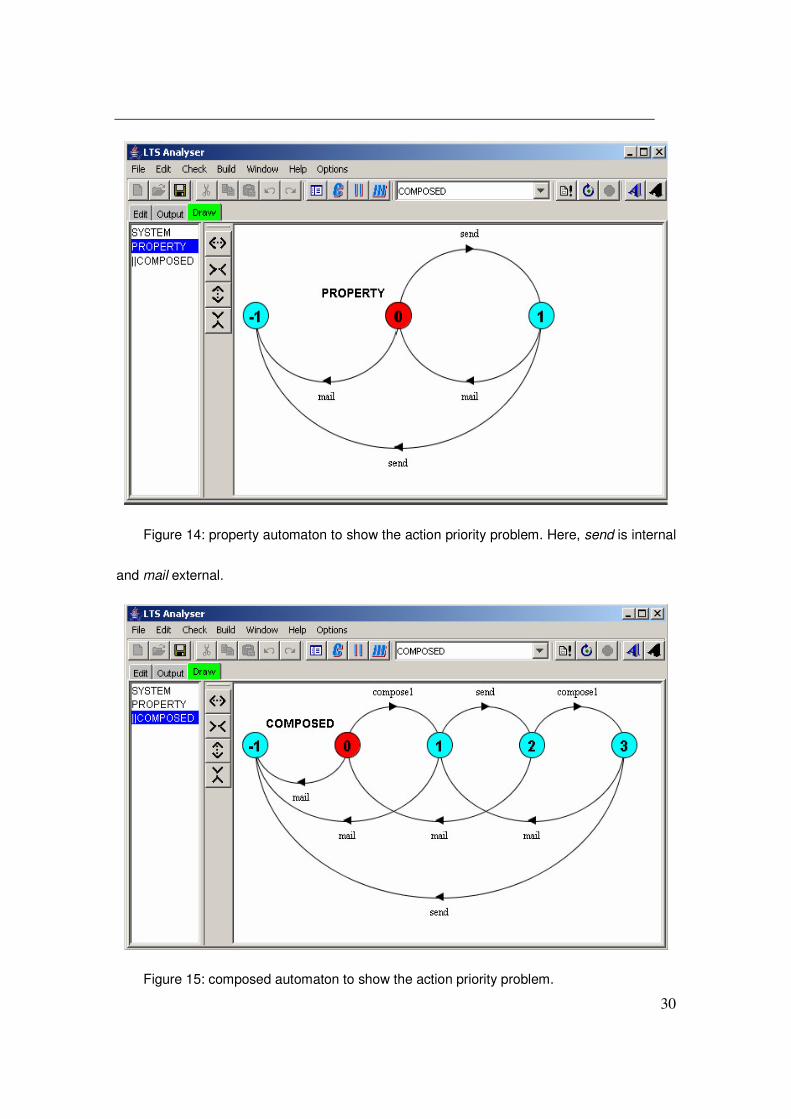
The property automaton in Figure 14 requires that the two actions send and mail
must be performed as an infinite sequence send->mail->send…….
30
Figure 14: property automaton to show the action priority problem. Here, send is internal
and mail external.
Figure 15: composed automaton to show the action priority problem.

31
The automaton in Figure 15 is the composition of the system and the property
without eliminating the internal actions compose1 and send. It defines both legal and
illegal traces.
In the next step, in order to remove the traces that can’t be prevented by the
environment from transitioning to the error state (the state labeled with -1),
Giannakopoulou’s method will propagate the error state to the state 3 in Figure 14 and
that’s where the conflicts happen. If we follow Giannakopoulou’s method faithfully, we
have to identify state 2 and state 3 as the error state and finally, we get nothing as
assumptions. But as a matter of fact, the environment can make the property true on the
system by performing the action mail after seeing send from the system. The problem
here is at these two states, both the component and the environment release some actions,
and then which one should the composed automaton take? We need some priority for
them. This is a nontrivial problem, especially for concurrent systems.
2.3.2 Properties
There’s huge difference between the properties that can be handled by the two
methods respectively. In general, Giannakopoulou’s method can process any property that
has a corresponding error LTS automaton, while Blundell's method handles full CTL; the
two are incomparable.

32
One major underlying assumption of Giannakopoulou’s method is that there exists an
error LTS automaton for the properties to be verified because her method relies on the
transitions to the error state. However, it is not always possible to do that for liveness
properties that require something expected must finally happen. A straightforward
example is (AG (AF f)) in CTL or (G (F f)) in LTL. There’s no way to build an error LTS
for it. This assumption limits Giannakopoulou’s method to handle mainly safety
properties and bounded liveness ones.
Secondly, all actions in Giannakopoulou’s method are exclusively true, i.e., only one
action can be true at any time instance and whenever an action is true, all others are set
false automatically. Since the properties in her method are expressed in terms of these
non-persistent actions, they are different with the common concept of properties from
other logics such as CTL, LTL, and CTL*. The differences we observed include:
1) Negation. There’s confusion arising if the property has negation of some action f
in it. The problem is when building the error LTS automaton, how to handle the
negation? One direct option is (!f = �-f) where � is the alphabet of the property
automaton, since the truth of any other action means the falsity of f. However
there may be some other actions from the system that are not in �. They can also
make f false, but are not known by the property automaton until composition.
There’s no way to take them into consideration in the error LTS automaton
construction.
2) And. Obviously, the exclusive characteristic of actions doesn’t allow the truth of
33
more than one action simultaneously. As a result, we can’t express properties like
(action1 ^ action2). This difference is important in that it dramatically narrows
the scope of properties that can be handled by Giannakopoulou’s method.
Giannakopoulou and Magee admit this non-persistent issue makes the task of
expressing properties often unmanageable and proposed an elegant and uniform solution
[1]. However, they haven’t integrated this solution into their assumption generation
research yet and that’s why I can’t analyze and evaluate it in my thesis.
Giannakopoulou’s method suffers from non-persistent actions, but a persistent world
like Blundell’s also suffer from another problem, that’s his persistent world can’t express
repetition. In a real system or protocol, it’s practical to expect something could happen
several times. For example, we may expect an email to be encrypted twice. This can be
easily expressed by the number of occurrence of some action in Giannakopoulou’s
method, but impossible by Blundell’s persistent world unless the proposition is explicitly
checked for false in between repetitions. Persistence, in Blundell’s world, comes from
data proposition. Obviously, as long as an email is encrypted, this attribute persists to be
true, even after it’s encrypted again, but there’s no way to express that something
persistent repeats in CTL.
2.4 Unifying the inputs & outputs of the two methods
34
In order to make a rigorous comparison, it’s ideal if we can
1) build equivalent systems
2) specify equivalent properties on the two systems
3) run the two methods
However, this is extremely hard, if possible. We can’t eliminate so many problems as
stated above especially in expressing properties. This is also partially because of the
current progress of Giannakopoulou’s method: she doesn’t have the solution to some
problems; for others, despite that she has some new progress, she hasn’t integrated them
yet. So, we can only do comparable case studies to learn these differences in the outputs
of the two methods. By “comparable”, I mean though we can’t ensure equivalent inputs
for the two methods, we can still build similar ones to discover the problems. But we
must make some important changes first.
2.4.1 Unifying inputs of the two methods
From previous sections, we know that Giannakopoulou’s and Blundell’s methods
adopt totally different automata to describe the input systems/features. Although the two
kinds of automata can be converted into each other, due to many subtleties such as the
characteristics of exclusive actions, finite and infinite executions and property
expressions as discussed before, we can’t use one model for both of them directly.
As a result, the first step for my comparison is to unify their input formats to
eliminate the gaps. Since “sequential” can be viewed as a special case of “concurrent” as

35
discussed at the beginning of this chapter, I tried to map Blundell’s inputs into
Giannakopoulou’s input format without affecting the actual executions.
Definition 4: FSM Input Conversion algorithm
Given a feature F1 expressed by a Moore Machine M that’s consumed by Blundell’s
method and another feature F2 to be executed after F1, we take the following steps:
1) Convert M into a Mealy Machine M’ [17], which is closer to the event-style
machine in Giannakopoulou’s method
2) Create a new state dummy
3) Add a transition from dummy to the starting state of M’ with startF1 as the
guard
4) Add a transition from each terminal state of M’ to dummy with startF2 as the
guard (terminal states refer to those states without any transitions going out.)
Figure 16 summarizes the input-unifying process:

36
Now we have an infinitely running system M’’ to input into Giannakopoulou’s
method for comparison. StartF1 and startF2 are indicators to start and terminate the
execution of M’. They don’t interfere with the actual execution of the automaton and
serve to make sure that at one time instance, no more than one feature is in its execution
phase. Besides, since they don’t provide useful information, they will be removed from
the final assumption automaton by being hidden as internal. startF1 and startF2 can also
have functionality: As we discussed in previous section about the drawbacks of actions,
Giannakopoulou’s method doesn’t work on a component if it has only internal actions.
The introduction of startF1 and startF2 can make her method handle more cases since
the two actions can serve as what the system uses for communication with the
environment.

37
2.4.2 Unifying outputs
Theoretically, Giannakopoulou’s method has the benefit of rendering us with
constraints for all possible cases, i.e., from components that run before, after and
concurrently with the current one, while Blundell’s temporal constraints are only for the
future features. Our experiments also support this. Figure 17-19 is such an example.
The system in Figure 17 fulfills three actions: getUserReq that gets user request,
compose1 that allows users to compose an email and inputAddr that asks users for
mailing address.
Figure 17: An email system where getUserReq is external and all others internal
38
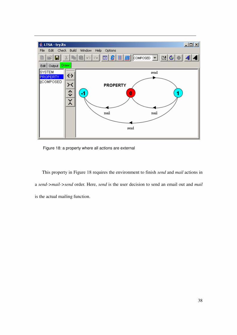
Figure 18: a property where all actions are external
This property in Figure 18 requires the environment to finish send and mail actions in
a send->mail->send order. Here, send is the user decision to send an email out and mail
is the actual mailing function.
39
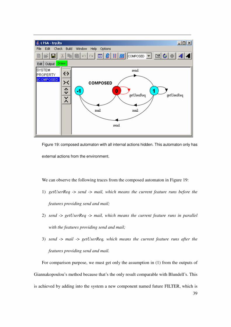
Figure 19: composed automaton with all internal actions hidden. This automaton only has
external actions from the environment.
We can observe the following traces from the composed automaton in Figure 19:
1) getUserReq -> send -> mail, which means the current feature runs before the
features providing send and mail;
2) send -> getUserReq -> mail, which means the current feature runs in parallel
with the features providing send and mail;
3) send -> mail -> getUserReq, which means the current feature runs after the
features providing send and mail.
For comparison purpose, we must get only the assumption in (1) from the outputs of
Giannakopoulou’s method because that’s the only result comparable with Blundell’s. This
is achieved by adding into the system a new component named future FILTER, which is

40
basically an error LTS automaton.
Definition 5: A future FILTER for a property is constructed as follows:
1) Given a property automaton, we can hide and eliminate all internal actions to get an
automaton P’ as Giannakopoulou’s method does
2) Create an automaton T with two states s1 and s2 where s1 transits to s2 on startf1
3) Compose the two automata, P’ and T, into a new one F in this way: first, add a
transition from s2 to the starting state of P’ with startf2 as the guard; second,
originally each terminal state of P’ has one or more transitions to the starting state, but
now change s1 to be the destination of all these transitions.
4) Make F complete by adding all missing transitions to a special error state.

41
Figure 20 is the graphical flow of constructing a future FILTER. Note that the special
error state is not shown here for simplicity.
We can also use startF1 and startF2 as delimiters. Any action that happens before
startF1 is supposed to be from the previous features and any action that happens after
startF2 is supposed to be from the future features. Since a future FILTER places all other
external actions after startf2 and startf2 and takes all other possible orders of external
actions as violations, composing a future FILTER with the system and the property
automatons in Giannakopoulou’s method will get the assumptions for the future features
out.
Note that though so far it’s not clear how to build a minimal future FILTER, I believe
the solutions are not necessary at all. This is because the intention here is trying to do the
comparison, the performance issue of the comparison algorithm is not important.
2.5 Summary of case studies
A number of examples that cover all possible FSM structures (including branches &
cycles) and 14 possible property structures (different positions for internal and external
actions) have been done to compare and analyze the two methods. The outputs and the
detailed analysis are in the appendix. In this section, a table summarizes the major points
of the case studies and the expectation of my own method:

42
Generating interfaces for components
Giannakopoulou’s method
Blundell’s method Expectation for my new method
My reasons
Interfaces for what purpose?
Verify property for concurrent systems
Verify property for sequential systems
Verify property for sequential systems
Our motivation
How are the interfaces used?
LTS automata composition (Env||Assumption)
Discharging by data environment
Doesn’t matter
What’s the problem domain?
Component -based SE (CBSE)
Feature-Oriented SE
Doesn’t matter, but it should also be a modular method
What’s the input?
LTS automata Propositional & CTL constraints
Propositional & CTL constraints
Automata determination may cause state explosions
What’s the output?
LTS automata Propositional & CTL constraints
Propositional & CTL constraints
Be uniform with the input, if no other benefits
What’s the composition assumption?
Concurrent Sequential Sequential My thesis motivation
What is the architecture assumption?
The system model is basically a cycle.
A terminal state has no direct descendent inside a feature and no cycles in feature composition.
Allow circular confections.
Obvious
What is the system model assumption?
State transitions are described by actions that are non-persistent, and only one of the system and the environment can release an action
Variables/propositions at each state.
Variables/propositions at each state.
They’re persistent. Each module is free to use a proposition that’s also used by others modules. They provide a better system model.
What is the property assumption?
Must has a corresponding error LTS automata
Can be expressed by CTL.
Can be expressed by CTL.
CTL matches well with the system model with state variables.

43
The fourth column describes briefly how my method looks like from a high perspective
and the fifth column gives justifications for my decision. Obviously, this table indicates
that I should choose Blundell’s method as the foundation of mine.

44
Chapter 3
An abstraction-based modular verification method
The basic idea of my method is to build abstract states for each feature and the base,
compose them into an abstract FSM based on the original state/feature connections, and
then apply a variant of the traditional CTL model checker on this abstract FSM to verify
the property.
3.1 Formal models of the abstract Finite State Machines (FSM)
Before showing the details of the abstraction-based modular model checking method,
I give the formal definitions of the fundamental elements in this method.
My method also works for feature-oriented sequential systems and I reuse some of
Blundell’s work. My definitions of features, the base, the product and the data
environment given in Chapter 1 are the same as Blundell’s, but I have a different
definition for feature connection relationships (refer to Definition 3 in Chapter 1) because
my method allows cyclic feature compositions. In addition, I also define the following
new terms.
Definition 6: A Label Set (LS) is a set of CTL formulas including both atomic

45
propositions and non-atomic formulas in the form of (fmla, val) where val is the value of
the formula fmla that may be one of the following three forms:
1. Boolean value
2. � that means either true or false
3. Non-atomic formula
Obviously, the major difference between my LS and the label set in the traditional
FSM comes from the possible value of fmla.
There will be one LS per abstract state, generated based on both the feature and the
property using the first phase of Blundell’s method that analyzes the property pty against
each feature by traversing from the starting state to each terminal state of a feature
separately. In this process, some sub-formula fmla of pty may be fully analyzed, i.e., their
values can be decided without information from neighboring features, while other
sub-formulas may be partially analyzed, i.e., only the value of some sub-formula f’ of f,
but not f itself, can be decided. For example, given f = (f’->EFsth) where f’ is true but sth
unknown in a path inside a feature, we get f’’ = EFsth as the partially analyzed result of f
on this path.
Definition 7: An Abstract State is a state annotated with a Label Set (LS).
Note that similar as the LS, abstract states are also built one per terminal state of the
feature. Abstract state and LS form corresponding pairs.
46
As a matter of fact, the only difference between an abstract state and a state in
traditional FSM comes from the state labels: the former uses the LS while the latter uses
propositions and fully analyzed formulas.
Definition 8: An Abstract Finite State Machine (FSM) is a finite state machine
constructed by connecting abstract states via directed edges.
An abstract FSM is almost the same as the traditional FSM expect the different state
labels at their states.
In Chapter 1, I defined the feature and the base separately as different concepts, but
in my verification method, their difference is irrelevant and I treat the base just as a
feature with special structures. Thus I define the splitting algorithm to split the base into
two features so that my method can process the base and the features in a uniform way.
Definition 9: The splitting algorithm works as follows:
Let s0 be the initial state of the base, sbt be the state where there are edges coming
from other features into the base and sb be the state where there are edges coming from
the base into other features. Although actually there may be more than one sb, I assume
it’s unique for simple discussion. Let’s also assume the base is connected with a series of
F0…Fi via (sbt, sb). The base is then split into the following two features (FSM):

47
1) F0: starting from s0 to sbt, put all reachable states, as well as their transitions, into
an FSM
2) Fi+1: starting from sb, put all reachable states, as well as their transitions, into an
FSM
3.2 An abstraction-based model checker
In this section, I will introduce my new model checking method on the abstract FSM
by going through an email system example. Figure 21 shows the system that I will use as
an example. The property to be verified is also indicated in this figure.
48
Phase 1: Partially analyze the property on each feature to construct the Label Sets
The first phase of my method is almost the same as the first phase in Blundell's,
which does a partial analysis on each feature and labels each terminal state of a feature
with constraints and a data environment (DE). Let’s denote this process as Gen-Cons(F,
pty) where F is a feature and pty the property. In Figure 21, the data environments are {(f1,
true), (f2, true)} and {(f1, true), (f2, false)} for the two terminal states of F1 respectively,
{(f2, true)} for the terminal state of F2 and {(f1, false)} for that of F3. The constraints for
fi are what the adjacent features must guarantee for the property to hold on fi. The results
of Blundell’s constraint generation, denoted as the Constraint Sets (CS), for the three
features are:
1) (EGf3^ pty) for the terminal state of F1 where both f1 and f2 are true and (EFf2^
EGf3^ pty) for the other terminal state of F1 where f1 is true and f2 false
2) (((f1 ^ EGf3) v (!f1)) ^ pty) for the terminal state of F2 where f2 is true
3) pty for the terminal state of F3 where f1 is false
My method also applies the splitting algorithm to divide the base into two features F0
and F4 and generates constraints for them:
4) (((f1 ^ f2 ^ EFf3) v (f1 ^ !f2 ^ EFf2 ^ EFf3) v (!f1)) ^ pty) for the state that is directly
connected with F2 in the base.
5) (((f1 ^ (f2 v (!f2 ^ EFf2)) v (!f1)) ^ pty) for the state, denoted as sb, that is directly
connected with F2 in the base.

49
The constraints in CS have both propositional parts for the preceding features, such as
f1 in the constraints for F2 and temporal parts like (EGf3^ pty) for the subsequent features.
My method put the pairs composed of the sub-formulas and their corresponding
constraints into the LS:
1) {(pty, (((f1 ^ f2 ^ EFf3) v (f1 ^ !f2 ^ EFf2 ^ EFf3) v (!f1)) ^ pty))} for the terminal
state in F0
2) {(pty, EGf3^ pty), (EFf2, true), (EGf3, EGf3)} and {(pty, EFf2^ EGf3^ pty), (EFf2,
EFf2), (EGf3, EGf3)} for the two terminal states of F1 respectively
3) {(pty, (f1 ^ (EGf3^ pty)) v (!f1 ^ pty)), (EFf2, true)} for the terminal state of F2
4) {(pty, pty)} for the terminal state of F3
5) {(pty, ((f1 ^ (f2 v (!f2 ^ EFf2)) v (!f1)) ^ pty)), (EGf3, true)) for sb of F4
Note that I only list some temporal sub-formulas here for simplicity. The non-atomic
sub-formulas with logical connectives as the outmost operators can be constructed from
these temporal ones fairly easily.
Phase 2: Propagating the data environment (DE) & removing the propositional
constraints in CS
The data propositions are expected to persist over multiple states but the above FSM
can't reflect that. So we need to propagate the data propositions from the DE of a

50
predecessor feature to the DE of all its successor features starting from F1. The following
defines how to do that:
1) It's possible for a feature or the base to have multiple DE coming from its
predecessor features. In that case, I combine all these DE first to get a new DE'.
If different DE set a proposition to be different values, I store (prop, �) into DE',
which mean prop may be either true or false at different time instances
depending on the specific program executions. At the end there's only one
predecessor DE' for each feature to use. For the starting feature F0, we also
count a special DE, where all data propositions are initiated to be false, as a
predecessor DE to capture the fact that all data propositions are initially false
and remain false unless assigned true explicitly.
2) Update the DE at each feature and the base. Specifically, for any data
proposition occurring in the DE' but not the DE of the current feature, put a
copy of this proposition and its value into the DE; for those occurring in the DE,
keep their up-to-date values. Finally, delete DE'.
Example:
Following the above rules, we have DE01{(f1, false), (f2, false), (f3, false)}, DE11{(f1,
true), (f2, true), (f3, false)}, DE12{(f1, true), (f2, false), (f3, false)}, DE21 {(f1, �), (f2,
true), (f3, false)}, DE31{(f1, false), (f2, true), (f3, false)} and DE41 {(f1, �), (f2, true), (f3,
true)}. Now, all data propositions are known at every feature, despite their values may

51
not be solid true or false. The fact that the value of a known proposition may be �
indicates that the value of such a data proposition at a state may be different if the system
is executed along different paths.
Remember that we generate temporal constraints based on the possible values of
those unknown propositions. Since in this propagation phase, the actual values of some
unknown propositions become known, we can also further analyze the constraints in the
LS according to what the actual values of the propositions are. Such constraints based on
true/false propositional assumptions after that has only temporal parts. For example, if we
have a constraint (f, (f ^ f’) v (!f ^ f)) and the propagated DE shows f is true, then the
constraint can be further analyzed as (f, f’).
In phase1, I listed the constraints for all features and keep them in the LS. At this
phase, they are updated as follows:
1) {(pty, pty)} for the terminal state in F0
2) {(pty, EGf3^ pty), (EFf2, true), (EGf3, EGf3)} and {(pty, EFf2^ EGf3^ pty), (EFf2,
EFf2), (EGf3, EGf3)} for the two terminal states of F1 respectively
3) {(pty, (f1 ^ (EGf3^ pty)) v (!f1 ^ pty)), (EFf2, true)} for the terminal state of F2
4) {(pty, pty)} for the terminal state of F3
5) {(pty, pty)), (EGf3, true)) for sb of F4
Phase 3: An abstract system model
The abstract system model is built as follows:

52
1) Create a graph with one node per terminal state of each feature.
2) Add edges between nodes capturing transitions between these terminal states
within a feature.
3) For any two features fi and fj that are directly connected by some transitions, add
edges between their corresponding nodes capturing these transitions.
4) Name each node as sij, where i refers to a feature and j refers to a terminal state of
the feature.
5) Set the LS of each sij to be the one of the terminal state correspondent to sij.
6) Insert all data propositions and their values in the starting state of fi into the LS of
each sij. Note that the value of such a data proposition may be �, which means it
may be either true or false depending on the actual program executions.
Example:
Figure 22 is the diagram of the abstract FSM of my example after this phase:
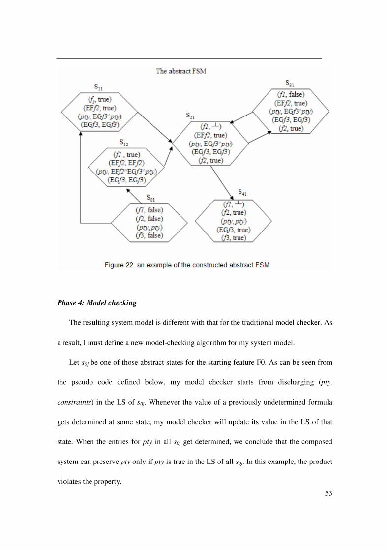
53
Phase 4: Model checking
The resulting system model is different with that for the traditional model checker. As
a result, I must define a new model-checking algorithm for my system model.
Let s0j be one of those abstract states for the starting feature F0. As can be seen from
the pseudo code defined below, my model checker starts from discharging (pty,
constraints) in the LS of s0j. Whenever the value of a previously undetermined formula
gets determined at some state, my model checker will update its value in the LS of that
state. When the entries for pty in all s0j get determined, we conclude that the composed
system can preserve pty only if pty is true in the LS of all s0j. In this example, the product
violates the property.

54
The major differences between my Abstraction-based Model Checker (AMC) and the
Traditional Model Checker (TMC) include:
1. TMC uses Boolean logic, but since AMC have the � value, I must have a
three-valued logic [18][19] and all evaluation of propositional formulas must be
able to handle �, as shown in the Truth Table for AMC below.
2. If the LS has a value for a formula, AMC does not check its sub-formula, unlike
TMC which checks all sub-formulas.
3. Instead of checking the state propositions and labels as TMC does, AMC checks
the LS at each abstract state.
Note that AMC uses the same logic and resembles TMC greatly in the processing of
the logical connectives and temporal operators, as shown in the pseudo code.
The rest of this section presents the truth tables that underlie three valued model
checking and present the pseudo code for the model checker. Truth table for AMC: OR True False � F’ True True True True True False True False � Val(f’) � True � � � OR Val(f’) f* True Val(f)* Val(f) OR � Val(f) OR Val(f’) *f means a non-atomic formula and Val(f) means the value of f after being fully analyzed. AND True False � F’ True True False � Val(f’) False False False False False � � False � � AND Val(f’) f* Val(f) False Val(f) AND � Val(f) AND Val(f’)

55
NOT True False False True � � f* NOT(Val(f))
Pseudo Code for AMC ;; consume a state s and a formula/proposition f to return the value of f in the LS of s. ;; if the formula/proposition has an entry in the LS, ;; the return value maybe true, false, � or some constraint; ;; else, the formula doesn’t have an entry in the LS and the function returns N/A function get-val(s, f) { return the value of f in the LS of s;} ;; consume a state and a formula, label this state with the value of the formula function AMC_help(s, f) { if get-val(s, f) returns a value val, return val; else {for each immediate sub-formula f ’ of f, AMC(sm, f’);} if the outmost operator of f is EX, EU, use the original TMC_help function to decide
the value of f based on the labels in the LS; if the outmost operator of f is EG, for all desc-state-s, the descendent states of s, check
TMC_help(desc-state-s, EGf), f is true at s only if at least one of these TMC_help(desc-state-s, EGf) functional calls returns true;
else if the outmost operator of f is ^, v, or !, use the Truth table for abs_TMC as defined later;
update the value of f in the LS; } ;; consume a finite state machine and a formula, label the formula ;; in the states of the FSM function AMC(sm, f) { for each s � sm, AMC_help(s, f)} ;; consume a state s and a formula in the LS of s to fully analyze it

56
function dischargeFmla(s, f) { temp = get-val(s, f); if temp is true or false or �, return temp; else // f is a formula(or constraint) AMC(s, temp);} ;; consume an abstract FSM in which each state is labeled with an LS, ;; fully discharge the LS of the abstract states of the starting feature. function MC_FSM ( aFSM) {
for each state s1i { val = dischargeFmla(s1i, pty);
if val == false, return false; else if val == �, return �;} return true;}

57
Chapter 4
Soundness Proof
In this section, outline of the proof about the soundness of my model checker is given.
First of all, I give definitions of some terms used in this chapter.
The outline depends on a machine called the propagated product Ppg that is a version
of product P with data proposition values propagated.
Definition 10: Given a product and a formula to be verified, let Apg be the abstract
FSM built in the third step of my method.
Note that Apg is built based on not only the product but also the property. In other
words, if the property is changed, Apg should also be changed correspondingly.
My goal is to prove the following Core Theorem, in which I use the traditional model
checker as the standard to show the soundness of my method.
Core Theorem:
Let the traditional model checker be TMC(Ppg, pty) where Ppg is a propagated

58
product and pty a formula. Then
1) TMC(Ppg, pty) returns true if MC_FSM( BuildAbsFSM(Ppg, pty)) returns true
2) TMC(Ppg, pty) returns false if MC_FSM( BuildAbsFSM(Ppg, pty)) returns false.
Here, function MC_FSM refers to my abstraction-based model checker and the
function BuildAbsFSM denotes the process of building an abstract FSM for a product
according to the desired property.
In order to prove the Core Theorem, I have to use the following two theorems from
Blundell.
Blundell’s Theorem 1:
Let F1 and F2 be features, s be a state in F1, and � a CTL formula. Let V be a data
environment coming into F1 and F1V be F1 augmented with V. Let c be the result of
CONSTRAIN(F1, f, s), the constraint generation function call. Let Cr be c with every
annotated formula fst replaced with the value of �(true, false, �) in the initial state of F2
with which st connects. Let � be the feature connection relationship that is sequential and
doesn’t permit cycles between features. Then
1) F1V � F2, s |= f if V satisfies Cr
2) F1V � F2, s |= !f if V doesn’t satisfy Cr
This theorem states that if the constraints can be satisfied by the incoming data

59
environment and the formulas from the following features, then f, the desired property,
holds in the system composed by F1, F2 and V.
Blundell’s theorem 2*(Soundness):
Let P be the product, and P' be P augmented with the empty data environment (all
data propositions of the product set to false). Let SUBS be the function from initial states
and sub-formulas of f to the set {true, false, �} that stores the results of checking each
constraint under the composed data environments and the verified subsequent features.
Let f be the property to be verified and f1 be a sub-formula of f. Let Fi be a feature in P,
and s0 an initial state of Fi. Let � be the feature connection relationship that is sequential
and doesn’t contain cycles. Then:
1) Fi � Fi+1 �... � B, s0 |= f1 in the data environment of B � F1 �... � Fi-1
if SUBS[s0, f1] = True
2) Fi � Fi+1 �... � B, s0 |= !f1 in the data environment of B � F1 �... � Fi-1
if SUBS[s0, f1] = False
*: this theorem has been simplified here by removing some irrelevant terms
Basically, this theorem states that whenever SUBS returns true/false in checking a
sub-formula f1 of f (the property to be verified), TMC(f1, s0) on Ppg also returns
true/false.

60
Since my method builds the abstract states with LS in isolation and connects these
states into a FSM, I must show that the values stored in the LS are still valid once features
are composed into a product.
Key Lemma:
If f is a fully analyzable formula in the LS of an abstract state, then its value at the
corresponding terminal state is still accurate after the features are composed into a
product.
Proof:
Let’s analyze all possible forms of such a fully analyzable formula f:
1) f is a Boolean proposition. In this case, obviously, the value of a proposition
won’t change after state composition.
2) f is a non-atomic formula with EX, EU or EG as the outmost operator. In this case,
since composing abstract states together doesn’t remove any existing edge, the
value of f won’t change.
3) f is a non-atomic formula with AX, AU or AG as the outmost operator. We know
that the architectural assumption of my method is all non-terminal states can
transit to a terminal state, denoted as st, by one or more steps and each terminal
state is the last state to be visited in all feature execution paths. This means f
doesn’t need the values of any non-atomic formulas at st, which doesn’t have any
61
descendent states inside a feature. So, if f doesn’t need st to be fully analyzed,
composing states together won’t change its value; otherwise, � needs the Boolean
propositions at st to be fully analyzed and composing states together by adding
edges won’t change the values of propositions at st.
Therefore, Key Lemma holds.
In the following, I provide sketches of the proofs for the Core Theorem. My proof
outline starts with proving Theorem 1 first.
Theorem 1:
Core theorem holds when the product is composed of a set of features, denoted as
F1…Fi-1, and the base, which is split into F0 and Fi, the first and the last feature to be
executed in Ppg respectively, as defined in the construction of abstract FSM, and these
features are connected sequentially without any cycle in it.
Proof sketch:
Sequential connection means only one feature can be in its execution phase at any
time instance and a feature Fj starts execution only after its preceding feature Fi
terminates executions. According to this, a terminal state of Fi may be connected with
more than one initial state of other features and after the execution of Fi is done, one of

62
these next features will be activated based on the execution of Fi. Hence there may exist
branches in feature connections.
I assume given a pty to be checked, its value in the LS of s0’, an abstract state of F0
in Afsm, is f. The argument is by induction on the structure of the formula.
Remember that from Key Lemma, we know that LS still accurately reflects the
values of fully analyzed formulas.
Bases cases:
1) If f is an atomic proposition, the TMC will check the state variables at the starting
state s0 of F0 and my MC_FSM will check the atomic propositions in the LS of
all starting states s0’ of Afsm. Theorem1 holds since the atomic proposition set in
each starting state of Afsm is exactly the same as that in all the starting state of
F1 by construction.
2) If f is a non-atomic formula and is fully analyzed at some starting state s0’ of
Afsm, then MC_FSM will fetch its value directly out of the LS of s0’. The
true/false value of each formula in s0’ is generated from F0 by Blundell’s
Gen-cons(F0, pty) method. Since this function just records the details within a
feature, whether there exits a cycle in feature connections is irrelevant to the
values of formulas it generates. There’s no distinction between the fully analyzed
formulas in Blundell’s method and the corresponding LS in mine. Based on

63
Blundell’s theorem2, Theorem 1 holds.
Induction step: Assume this theorem holds for all f ’, those immediate sub-formulas
of f. Let’s analyze the possible forms of such a formula f:
The basic idea of my proof here is:
1) Prove that if MC_TMC assigns a value to f at s0’, then f is assigned the same
value at st, the terminal state of F0 that corresponds to s0’ in Ppg.
2) In MC_TMC, the value of pty is f in the LS of s0’. So, MC_TMC concludes pty
holds in Ppg if f is true at s0’ and pty is falsified otherwise.
3) According to Blundell’s Theorem1, if f true, pty holds; otherwise, pty doesn’t
hold on Ppg.
4) According to Blundell’s Theorem2 (Soundness), if pty holds, TMC also decides
that pty holds in Ppg; otherwise, TMC decides Ppg violates pty.
This means when MC_TMC decides pty is true in Ppg, TMC gets the same result and
therefore Theorem 1 holds.
Now, I must prove (1), which is defined as the following theorem.
Subsidiary Theorem:
Let s0’ be an abstract state of F0 in Afsm and f be the value of pty in the LS of s0’. If

64
MC_TMC assigns true/false to f at s0’, then f is true/false at st, the terminal state of F0
that corresponds to s0’ in Ppg.
Proof sketch:
1) f is EXf’.
In this case, if MC_TMC assigns true to f, f ’ must be true at some next state si’. By
construction of Afsm, the transition from s0’ to si’ mimics a transition between st and si,
the starting state of Fi.
• If f ’ is an atomic proposition, then f ’ is a state variable at si that has the same value
as at si’ by construction;
• If f ’ is a fully-analyzed formula when the Afsm was constructed, it’s a state label at
si that has the same value as at si’ by construction;
• Otherwise, f ’ was not fully analyzed at the construction time and MC_TMC
updates its value. Since we assume this theorem holds for f ’, TMC would also take
f ’ as a state label for si with the same value as MC_TMC assigns.
Hence, f must be true at st in Ppg in all these cases. Therefore, Subsidiary Theorem
holds in this case.
2) f is EGf’.
In this case, if MC_TMC assigns true to f, f ’ must be true in all states in a path from
s0’ to si’. Obviously, si’ is either a state visited more than once (i.e. loops) or an abstract
state of the base where the product terminates. By construction of Afsm, the transitions
65
from s0’ to si’ compose a series of features into a linear chain. We know that f summarizes
details inside features into abstract states, so if f is true at sj’, then f ’ is globally true at all
states in some path inside Fj. (Refer to the pseudo codes about how to processing EG.)
Since f is true in all sj’ in this linear chain, there must exist a path in Ppg that passes
through all these features and makes f ’ globally true. So, f must be true at st in Ppg.
Therefore, Subsidiary Theorem holds in this case.
3) f is E[f1’ U f2’].
In this case, if MC_TMC assigns true to f, there must exist a path from s0’ to si’ in
Afsm in which f1’ is always true from s0’ until f2’ is true at si’. I must show that in Ppg, f
must be true at st. This is done by contradiction. From the construction of Afsm, we know
that in Ppg there exists a path of concrete states from st for s0’…si’. Let’s assume the
corresponding path violated f and starting from st, the first violating state in this path is sj
in Fj. Since sj falsifies both f1’ and f2’ false, this implies that f is false at the starting state
of Fj and MC_TMC would conclude f is false when reaching this starting state. This
contradicts with the assumption that f is undetermined at Fj (and si’) and a further
checking of following features (states) is necessary. So, f must be true at st in Ppg.
Therefore, Subsidiary Theorem holds in this case.
4) f is !EXf’, !EGf’ or !E[f1’ U f2’].
Due to the architectural assumptions, Key Lemma tells us that the values of the fully
analyzable formulas won’t change after abstract state compositions and we can only add
new edges/transitions by connecting a terminal state of the current feature with the

66
starting states of next features. Consequently, the proofs of these cases are similar with
the first three cases respectively. The difference is when deciding the value of f, both
TMC and MC_TMC check if the expected sub-formulas occur in ALL paths from st or
s0’. Subsidiary Theorem still holds in this case.
5) f is (f1’ ^ f2’) or (f1’ v f2’).
In these propositional cases, since we assume Theorem 1 holds for both f1’ and f2’,
it’s straightforward that Subsidiary Theorem holds in this case.
Therefore, Subsidiary Theorem and Theorem 1 hold.
Next, I outline the proof of the Theorem 2.
Theorem 2:
Core theorem holds when the product is composed of a set of features and the base,
which is split into F0 and Fi+1, the first and the last feature to be executed in Ppg
respectively, as defined in the construction of abstract FSM, and these features are
organized sequentially, denoted as F1…Fi, with cycles in it.
Proof sketch:
There can be only one type of cycles in the feature compositions: cycles that flow
from Fi to Fj where Fi is different with Fj. (Self-loop on a feature should be regarded as

67
internal details instead of external connections.)
The proof is also done by induction on the structure of the formula:
Base cases: the base cases are the same as those in Theorem1, because in such cases,
pty can be fully analyzed on a single feature F0. They both just deal with the details
inside a feature and are irrelevant to the external feature connections.
Inductive step: The core part is still to prove Subsidiary Theorem. I only analyze
how the cycle may impact the process of deciding the value of f here for simplicity and
all other parts of the proof are identical with those in the Inductive step in proving
Theorem1. The following are proofs for the Subsidiary Theorem for this theorem:
1) f is EXf’.
In this case, the circular connections pose no impact. Cycles only matter with paths,
so EX shouldn’t get affected. Hence, Subsidiary Theorem holds in this case.
2) f is EGf’ or E[f1’ U f2’].
In this case, the path that has a cycle in Afsm mimics a concrete path in Ppg that has
a cycle going from a feature Fj back to a previous visited feature Fi. MC_TMC halts on
this path when hitting the visited state again and decides the value of f in the same way
(refer to function abs_TMC_help(s, f) in the pseudo codes in previous sections) as TMC
handles the concrete path in Ppg. So, the two corresponding paths in two methods still

68
guarantee the same true/false results. Hence, Subsidiary Theorem holds in this case.
3) f is !EXf’, !EGf’ or !E[f1’ U f2’].
These cases are also based on the first three cases respectively. Due to the
architecture assumptions, based on Key Lemma, the only difference is still when deciding
the value of f, both TMC and MC_TMC check if the expected sub-formulas occur in ALL
path from st or s0’. Subsidiary Theorem still holds in this case.
4) f is f1’^ f2’ or f1’ v f2’.
The circular feature connections are irrelevant to this case, because both methods
only look at the current state (either an abstract state or a concrete one). By construction
of the LS, it’s straightforward that Subsidiary Theorem holds in this case
.
Therefore, both Subsidiary Theorem and Theorem 2 hold.
Finally, I prove Core Theorem based on Theorem 1 and Theorem 2.
The proof is immediate, since I have analyzed all possible forms of feature
connections and all possible structures of formulas. Core Theorem holds.
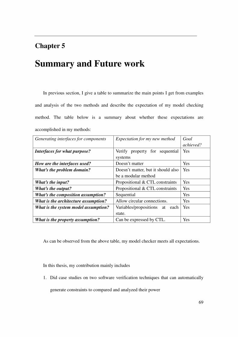
69
Chapter 5
Summary and Future work
In previous section, I give a table to summarize the main points I get from examples
and analysis of the two methods and describe the expectation of my model checking
method. The table below is a summary about whether these expectations are
accomplished in my methods:
Generating interfaces for components Expectation for my new method Goal achieved?
Interfaces for what purpose? Verify property for sequential systems
Yes
How are the interfaces used? Doesn’t matter Yes What’s the problem domain? Doesn’t matter, but it should also
be a modular method Yes
What’s the input? Propositional & CTL constraints Yes What’s the output? Propositional & CTL constraints Yes What’s the composition assumption? Sequential Yes What is the architecture assumption? Allow circular connections. Yes What is the system model assumption? Variables/propositions at each
state. Yes
What is the property assumption? Can be expressed by CTL. Yes
As can be observed from the above table, my model checker meets all expectations.
In this thesis, my contribution mainly includes
1. Did case studies on two software verification techniques that can automatically
generate constraints to compared and analyzed their power

70
2. Developed a new modular model checking method for cyclically composed open
features
3. Proved the soundness of my method
My method still assumes that a terminal state has no direct descendent state except
itself inside a feature. This inherits the assumption in Blundell’s constraint generation
method, which takes terminal states as terminating points for constraint generation and
hence his method doesn’t check states after the terminal ones. Both methods also assume
all non-terminal states can transit to a terminal state by one or more steps.
The performance of my abstraction-based approach relies on the costs both in
applying the first phase of Blundell’s method to partially analyze individual features and
in applying the revised abstraction-based model checker on the abstract FSM. The former
is a light weight process and so is the latter because the number of states in the abstract
FSM is not supposed to be large. Hence, my method is expected to be generally efficient.
Despite of not having validated my method in real software system designs, I have
done examples on small designs and property structures and I have confidence in my
method. Our future work includes
1. The implementation of my method.
2. Doing more case studies of my method using telecommunication feature designs

71
and systems [13].
3. Extend Blundell’s first phase to handle more system structures. This is the major
factor that limits the power of my method to handle more cases.

72
Bibliography [1] E.M.Clarke, E.A. Emerson, and A.P. Sistla. Automatic verification of finite-state concurrent systems using temporal logic specifications. ACM Transactions on Programming Languages and Systems, 8(2):244- 263, 1986. [2] M.Y. Vardi. An automata-theoretic approach to linear temporal logic. In F. Moller and G. Birtwistle, editors, Logics for Concurrency: Structure versus Automata, volume 1043 of Lecture Notes in Computer Science, pages 238-266. Springer-Verlag, Berlin, 1996. [3] Colin Blundell, Kathi Fisler, Shriram Krishnamurthi, and Pascal Van Hentenryck. Parameterized interfaces for open system verification of product lines. International Conference on Automated Software Engineering(ASE), 2004. [4] D. Giannakopoulou, C. Pasareanu, and H. Barringer. Assumption generation for software component verification. Proc. of the 17th IEEE International Conference on Automated Software Engineering (ASE 2002), 2002. [5] Ken McMillan. Circular compositional reasoning about liveness. IFIP Conference on Correct Hardware Design and Verification Methods, 342--354, 1999. [6] Martin Abadi and Leslie Lamport. Conjoining specifications. ACM Transactions on Programming Languages and Systems, 17(3):507--534, 1995. [7] David E. Long. Model-checking, Abstraction, and Compositional Verification. PhD thesis, Carnegie Mellon University, 1993. [8] Aspect oriented programming(article series). Communications of the ACM, 44(10), Oct. 2001. [9] Don Batory, Clay Johnson, Bob MacDonald, and Dale von Heeder. Achieving extensibility through product-lines and domain-specific languages: A case study. ACM TOSEM, April 2002. [10] C. Reid Turner, Alfonso Fuggetta, Luigi Lavazza, and Alexander L. Wolf. A conceptual basis for feature engineering. International Conference on Automated Software Engineering, 49(1):3--15, 1999. [11] D. Batory. Product-line architecture. In smalltalk and Java Conference, Oct. 1998.
73
[12] Christian Prehofer. Feature-oriented programming: A fresh look at object-oriented programming. In European Conference on Object-Oriented Programming, number 1231 in Lecture Notes in Computer Science, Springer-Verlag, 1997. [13] Pamela Zave. Calls considered harmful' and other observations: A tutorial on telephony. Services and Visualization: Towards User-Friendly Design, Lecture Notes in Computer Science 1385, Springer-Verlag, pages 8-27, 1998. [14] H. Peng, S. Tahar A Survey on Compositional Verification. Technical Report, Concordia University, Department of Electrical and Computer Engineering, December 1998. [15] Don Batory, Bernie Lofaso, and Yannis Smaragdakis, JTS: Tools for Implementing Domain-Specific Languages. 5th International Conference on Software Reuse, Victoria, Canada, June 1998. [16] John Hatcliff, Matthew B. Dwyer and Hongjun Zheng, Slicing Software for Model Construction, Journal of Higher-order and Symbolic Computation, 13(4), Dec. 2000. [17] Arto Salomaa, Theory of automata, Oxford, New York, Pergamon Press,1969 [18] M. Chechik, S. M. Easterbrook, and B. Devereux. Model checking with multivalued temporal logics. In Proceedings of the International Symposium on Multiple Valued Logics, 2001. [19] G. Bruns and P. Godefroid. Model checking partial state spaces with 3-valued temporal logics. In International Conference on Computer-Aided Verification, number 1633 in Lecture Notes in Computer Science, pages 274-287. Springer-Verlag, 1999.

74
Appendix A: Case study & Problems found In Section 2.4, I have done considerable amount of work to figure out how to make preparations for comparison. This appendix is devoted to running examples of Blundell’s and Giannakopoulou’s method to support my analysis. I documented the examples, results and problems found here. Please refer to the output comparison table for details about the examples and their outputs from the two methods. Part 1: Example selection I can’t guarantee the equivalence of the inputs to the two methods, for the problems discussed in Section 2.3. I can only define properties of the same structure and look at how the outputs differ. But the questions are 1. What kind of systems I should select as examples and 2. What kinds of properties I should select as examples. It’s pretty easy to find answers to question 1. My examples cover all possible system structures including linear chain, branches and cycles. The answer to question 2 is based on the interleaving of system actions and environment actions in the property. Let’s use S to denote actions from the system and E to denote actions from its environment. Giannakopoulou’s method uses S and E to describe the properties and the system. My selection of property examples is then based on the positions of the actions from S and E in the property. In the following, the examples are expressed by S and E. For example, SS means the property is composed of two actions from the system and ESE means the first and the last actions are from the environment and the action in the middle is from the system. Moreover, SS-c means there exists cycles in the example system and a name without “-c” refers to examples without cycles. Part 1: When purely S or there exists an S happening before all E in the property 1. SS PROBLEM FOUND: different definition of ‘open system’ ANALYSIS & REASON:

75
In Giannakopoulou’s method, this is really a “HOLD-FOR-ALL” case, which means the property holds on the component no matter what the environment does, and the final assumption is empty after hiding startF1 and startF2. In this example, the external action set is empty, hence the system is closed and her method generates nothing. But from Blundell’s method, we get (AG f)_st. The difference lies in the different definition of “open system”. Please refer to section2.1.1 for more explanation. 2. SE and SSE PROBELM FOUND: no problem found However, a further analysis of this example can help improve our understanding of the capability of the two methods in generating constraints for the future. 1. The constraints from Blundell’s method are the combination of the data environment,
which keeps all data proposition values of preceding features, and the partially analyzed constraints for the future features.
2. The final assumptions from Giannakopoulou’s method only include the trace for the future component.
ANALYSIS & REASON Blundell’s method utilizes the data environment to generate the partially analyzed constraints. Since he adopts persistent data propositions, the generation of these partially analyzed constraints is influenced: basically, Blundell’s method looks up the truth table of all the unknown propositions, find those valuations that can possibly make the property hold and generate corresponding temporal constraints. For example, (f1 -> AF f2) with f2 unknown will generate ( (!f2 ^ AF f2) v f2) as partially analyzed constraints. The value of f1 in previous features, despite not available at the first step, affects the generation of the temporal part. Giannakopoulou’s method can generate constraints from various environments freely. But for the introduction of FILTER, the final assumptions only include strictly those for the future. 3. SS-c PROBLEM FOUND: Giannakopoulou’s method generates wrong outputs For the different definitions of ‘open system’, Giannakopoulou’s method should have taken this example as a ‘closed system’ and a “FAIL-FOR-ALL” case, which means no matter what the environment does, the property fails on the component, but Blundell’s

76
should take this as an ‘open system’. 1. In the ‘closed system’ by Giannakopoulou’s method, we get some assumption trace,
which actually is what we need from the environment to drive the running of the branch that can preserve the property. Contradiction occurs here.
2. Blundell’s method succeeds in generating constraints based on what’s in each branches.
ANALYSIS & REASON: First of all, the final output of Giannakopoulou’s method is correct in terms of the property. But there’s some implicit point about the property. Without violating the truth of the property AG(S.busy -> AF S.fwd) or G(S.busy -> F S.fwd) in LTL, we can have as many busy actions as possible before the fwd action. But in order to construct an error LTS automaton, I assume the busy action can be release only once and after that we need to see fwd action eventually. Actually there are three branches totally in the system: one branch can preserve the property, one violates it and the last one vacuously preserves it. For the first branch, since no transitions to the error state happen in it, it will be left as the final assumption; For the second one, since in Giannakopoulou’s method the system is running infinitely, busy action will be released repeatedly and hence for the branch with busy but without fwd, it will definitely be trapped into the error state; The third one never sees busy and it can’t be synchronized with the property. However, I claim even if there was an error LTS automaton that could faithfully express the desired property, Giannakopoulou’s method would still fail. This is because, as stated in section 2.1.3, we have to specify fwd as an internal action so that the external environment can’t release it, then for the second branch, Giannakopoulou’s method takes it as violation since fwd can never be set true. Therefore, this is really an alphabet problem. Besides, we also need to remember that Giannakopoulou’s method aims at verifying property on open system, but the system in this example is closed with regards to the property. We are just doing some “extreme” case here. 4. SE-c and SSE-c PROBLEM FOUND: no However, it’s noteworthy to state that there’s difference between the outputs of SE and SE-c and SSE and SSE-c. Some constraints are missing in the complicated system design, due to the existence of cycles. Despite that these cycles don’t have data propositions in

77
them, they still can make the system fall into infinite loops and that’s why some valuations of the unknown propositions can’t serve as constraints. Part 2: When purely E or there exists an E happening before all S in the property This part is devoted to the cases when some proposition in the property is expected to happen before the current feature. When there exists some unknown proposition in the property that’s before all system actions, Blundell’s method would process all these cases in exactly the same way as processing SE/SSE. The temporal part in the partially analyzed constraints is also generated under assuming the possible valuations of the unknown proposition from preceding features based on their truth table. This is different with Giannakopoulou’s processing. Her outputs don’t refer to anything happening in the past, because the non-persistent actions don’t impact the current component. There may be questions arising since the constraints for the past have the same form as those for the future. Since the data environment is just a linear list to contain the up-to-date values of the data propositions, we may even suspect if this linear container is sufficient to keep the temporal relationships or not. These questions must be solved in the context of Blundell’s method: His method tries to work on individual features first to generate constraints. Whether a proposition in the property is known or unknown depends on which feature the method is working on. When there’s some unknown proposition happening in one feature f, this also means there must be some features preceding this one and take the unknown proposition as known. Hence, these preceding features take the responsibility of checking the temporal relationships between the unknown propositions in f and if there’s any violation of the property in some preceding feature f ’, f ’ will report false and failure of holding on any feature means the property can’t be preserved in the composed system. Therefore, we can safely push only the values of them into the data environment and pass it to the following features. 5. EE PROBLEMS FOUND: no ANALYSIS&REASON A property of EE structure means all propositions in the property are unknown to the current component/feature. So, they are either before or after the current component/feature.
1) For Blundell’s method. No matter whether both of the two propositions are supposed to be from the past or the future features or not, the constraints are the same. This comes from the persistent characteristic of the data propositions. If

78
they are from the past, their temporal relationship has been checked in preceding features and their valuations still impact the current feature; if they are from the future, their temporal relationships are also generated, as constraints for the following features, based on their valuation with false as default. The right values of the data propositions will be decided in the composition time.
2) For Giannakopoulou’s method. If we don’t use the future filter, the final assumptions have all possible cases, from the preceding, following and concurrent features. Adding a future FILTER will get the assumptions for the future out and similarly adding a past FILTER will get those for the past features out.
Comparing the two outputs, they provide the same information and both of them are correct in their context. 6. ES PROBLEM FOUND: no ANALYSIS & REASON: Compared with EE, this example will synchronize and eliminate the S action. Because of the structure of this property, when the S action happens, checking E action is not needed. Hence the outputs are about shifting the whole property to the following features because this is an AG property and the component is open. 7. ESE PROBLEM FOUND: no ANALYSIS & REASON: The S action gets synchronized with the component and eliminated. The two E actions are preserved in the same way as processing EE. 8. ESS PROBLEM FOUND: no ANALYSIS & REASON: Same as 6, the one for ES. 9. EE-c, ES-c, ESE-c, ESS-c PROBLEM FOUND: no ANALYSIS & REASON:

79
Compared with the examples of EE, ES, ESE and ESS, the FSM of these four have cycles. Cycles have the potential to make the system loop forever and affect the liveness property. We can observe that some possible valuations of the data propositions, together with their corresponding temporal constraints, are missing, compare with the examples without cycles. This is because they, if possible, will be trapped into the infinite loop so that something expected by the property won’t happen finally and the liveness can’t be satisfied.

80
Appendix B: The outputs of the 14 examples by the two tools
The following table defines 14 examples. Examples 8-14 are the complicated cases with
branches and cycles.

1
ID English Description CTL LTS NOTE & problems
CTL output LTS output File Name
1. 1) If the system is busy, then the incoming call should be forwarded finally and the busy signal should not come more than once.
2) Never forward if not busy.
3) Busy is turned on only once.
AG(busy -> AF fwd)
property P_CFBL = P0, P0 = (busy -> forward -> P0). (Implicit: Never forward if not busy && Busy is turned on only once)
A ‘HOLD-FOR-ALL’ case
AG(busy -> AF fwd)_st
Startf1->startf2->startf1 SS.lts
2 1) If an email is sign, then it’s finally mailed.
2) An email can be signed only once
3) An email can’t be mailed unless it’s signed.
AG(sign -> AF mail)
property P_SIGN = P0, P0 = (sign -> mail ->P0). (Implicit: An email can be signed only once && An email can’t be mailed unless it’s signed.)
(!mail ^ (AF mail)s3 ^ (AG (sign -> (AF mail)))s3 v ( mail ^ (AG (sign -> (AF mail)))s3 ) (depending on previous value of mail)
Startf1->startf2 ->mail->startf1
SE.lts

2
3 If an email is composed, then finally 1) It’s signed
and then eventually mailed.
2) An email can be signed only once.
3) An email can be composed only once.
4) Don’t sign until composed.
5) Don’t mail until signed.
AG(S.compose1 -> AF (S.sign -> AF E.mail))
property P_SIGN = P0, P0 = (compose -> sign -> mail -> P0). (Implicit: An email can be signed only once and can be composed only once)
(!mail ^ (AF mail)_s2 ^ (AG(compose -> AF (sign -> AF mail)))_s2 ) v (mail ^ (AG(compose -> AF (sign -> AF mail)))_s2 ) (Colin’s can generate redundancy in the constraints)
Startf1->startf2 ->mail->startf1
SSE.lts
4 1) If an email is signed or encrypted, it will be mailed finally.
2) An email can be signed/encrypted only once.
3) Never mail unless either encrypted or
AG((sign v encrypt) -> AF mail)
property P_TEST = P0, P0 = ({sign, encrypt}-> mail -> P0). (Implicit: An email can be signed/encrypted only once && Never mail unless either
1. The construction of the error LTS
and the negation of some action(s) bring so many implicit things.
2 EE can be before, after and
concurrent with the current feature. I
take the ‘after’ one
((sign v encrypt) ^ (mail v (!mail ^ (AFmail)_s2) ) ^ (AG f)_s2) v (!(sign v encrypt) ^ (AG f)_s2)
Startf1->startf2 ->{sign, encrypt} -> mail
EE.lts

3
signed encrypted or signed)
5 1) If an email is composed, it will be finally mailed.
2) Do not mail unless composed.
3) An mail is composed only once
AG( (compose -> AF mail))
property P_SIGN = P0, P0= (compose ->mail->P0 ). (Implicit: An mail is composed only once && Do not mail unless composed)
The same as 1. The difference is the first proposition is from Env
(AG(compose -> AF mail))_st
Compose->startf1->startf2->compose ES.lts
6 1) If an email is composed, it will finally be signed.
2) If 1) happens, the email will finally be mailed.
3) Don’t sign until composed.
4) Don’t mail until signed.
5) An email can be composed only once.
6) An email can be signed
AG( (compose -> AF (sign -> AF mail)))
property P_SIGN = P0, P0= (compose -> sign -> mail -> P0 ). (Implicit: 3-6 in the second column)
The construction of the error LTS and the negation of some action(s) bring so many implicit things.
(!compose ^ (AGf)_s7) v (compose ^ ((mail ^ (AFmail)_s7 ^ (AGf)_s7) v (!mail A (AGf)_s7)))
Compose -> startf1 ->startf2 -> mail -> compose
ESE.lts

4
only once.
7 The same as 6 AG( compose -> AF (sign -> AF mail ))
The same as 6 The difference is that both ‘compose’ and ‘mail’ are from Env.
AG( (compose -> AF sign) -> AF mail )_s4
Compose -> startf1 -> startf2 ESS.lts
8 The same as 1 The same as 1 The same as 1 Exception!! Expect “FAIL-For-All”, but get assumptions. Will also talk about branches.
((!busy ^ (( !fwd ^ (AF fwd)_s5) v fwd )) v(busy ^ ( (!fwd ^ (AF fwd)_s6 ^ (AF fwd)_s5) v fwd))) ^ (AG f)_s4 ^ (AG f)_s5 ^ (AG f)_s6)
startf1->startf2->startf1 (FAIL! Since the system is closed to Giannakopoulou’s and the property should be false on it.)
SS-c.lts
9 Same Results As 2 (sign ^ mail ^ (AG (sign -> AF mail))_s4) v (!sign ^ ( mail v (!mail ^ (AF mail)_s4)) ^ (AG (sign -> AF mail))_s4)
Startf1->startf2 ->mail->startf1
SE-c.lts
10 Same Results As 3 For the space limitation, I don’t write the complete constraints down
Startf1->startf2 ->mail->startf1
SSE-c.lts

5
here, but they are still based on all the possible valuations of the three prop, assuming they have values assigned in preceding features.
11 Same Results As 4(subset of 4) ((sign v encrypt) ^ mail ^ (AG f)_s2) v (!(sign v encrypt) ^ (AG f)_s2)
Startf1->startf2 ->{sign, encrypt} -> mail
EE-c.lts
12 Same Results As 5(subset of 5) (!compose ^ AG(compose -> AF mail)_s7 ) v (compose ^ mail ^ (!(!mail)_s7) ^AG(compose -> AF mail)_s7 )
Compose->startf1 ->startf2 ->compose
ES-c.lts
13 Same Results As 6(subset) (!compose ^ (AGf)_s7) v (compose ^ ((mail ^
Compose -> startf1 ->startf2 -> mail -> compose
ESE-c.lts

6
(AFmail)_s7 ^ (AGf)_s7))
14 Same Results As 7 (!compose v (compose ^ ( !sign v (sign ^ mail)))) ^ (AG( (compose -> AF sign) -> AF mail ))s8
Compose -> startf1 -> startf2 ESS-c.lts
Summary
Some of these properties are verified on the same feature. This is fine, since the feature provides them with the common case, the branches and the cycles

1