HAL Id: hal-01020451https://hal.inria.fr/hal-01020451

Submitted on 8 Jul 2014

HAL is a multi-disciplinary open accessarchive for the deposit and dissemination of sci-entific research documents, whether they are pub-lished or not. The documents may come fromteaching and research institutions in France orabroad, or from public or private research centers.

L’archive ouverte pluridisciplinaire HAL, estdestinée au dépôt et à la diffusion de documentsscientifiques de niveau recherche, publiés ou non,émanant des établissements d’enseignement et derecherche français ou étrangers, des laboratoirespublics ou privés.

A Modular SHM-Scheme for Engineering Structuresunder Changing Conditions: Application to an Offshore

Wind TurbineMoritz Häckell, Raimund Rolfes

To cite this version:Moritz Häckell, Raimund Rolfes. A Modular SHM-Scheme for Engineering Structures under Chang-ing Conditions: Application to an Offshore Wind Turbine. EWSHM - 7th European Workshop onStructural Health Monitoring, IFFSTTAR, Inria, Université de Nantes, Jul 2014, Nantes, France.�hal-01020451�

A MODULAR SHM-SCHEME FOR ENGINEERING STRUCTURES UNDERCHANGING CONDITIONS: APPLICATION TO AN OFFSHORE WIND

TURBINE

Moritz W. Hackell1, Raimund Rolfes1

1 Institute of Structural Analysis, Leibniz Universitat Hannover, Appelstraße 9A, 30169 Hannover

m.haeckell@isd.uni-hannover.de, r.rolfes@isd.uni-hannover.de

ABSTRACT

Many countries worldwide and in Europe still have the goal of a future cut of CO2 emis-sion in common. A shift from fossil to renewable energy source is the logical con-sequence. (Offshore) wind turbines ((O)WTs) play an important role in the so called”green” energy sector. An increasing number of remote offshore plants and an ageingfleet of onshore structures raise the demand of structural health monitoring (SHM) in thisfield. Guidelines still lack firm establishments and SHM is supposed to help assuring asafe operation and a possible extension of the lifetime.The work presented displays a modular SHM scheme applicable for engineering struc-tures under varying environmental and operational conditions (EOCs). The procedure isapplied to a 5MW OWT in the German bight, located in the test field alpha ventus. Theintegration into and application of the complete SHM scheme is presented through dif-ferent condition parameters (CPs), machine learning (data classification) and hypothesistesting.

KEYWORDS : Offshore Wind Turbine, Machine Learning, Condition Parameter,Control Charts, Affinity Propagation

INTRODUCTION

It is widely accepted that monitoring of large scale (civil engineering) structures’ necessitates ac-counting for the structures’ current state. In general, variations in the structures response are causedby variations in the environmental and operational conditions (EOCs). For (O)WT or bridges, thesecan be of diverse kinds as temperature (gradients), wind speed, turbulence intensity, traffic volume andtype and wave period and heights. All these influences may change the characteristics of the dynamicresponse and hence potentially the monitored condition parameter(s).

To achieve the task of monitoring a complex, large scale engineering structure, SHM faces dif-ferent difficulties. Not only two different states of the structure must be compared but all importantEOCs must be taken into account to represent all healthy conditions. Hence, for OWTs a learningphase is required to cover the differing behavior over yearly seasons. Next, type, location and extendof damage can vary strongly which leads to the intention that a single damage parameter might not besufficient for a good SHM performance. Last but not least, to be of use for owners and operators, themonitored parameters must be put into a probabilistic context and an intelligible layout. All of thesesteps are targeted here for the OWT.

In many cases, SHM is divided into four general, subsequent steps after Rytter [1]: Damage-detection, -localization, -quantification, and -prediction. While this is a general description of SHM-goals, their implementation remains open. To achieve the purposes of SHM, many different techniquesare available and clarification needs to be given on what purpose they are used for. Figure 1 shows themodular SHM-scheme applied. Four general (structure-independent) steps are displayed, which givethe tools to approach the (first two) SHM goals. Monitoring is divided into training and testing phase(dashed lines). Within the later one, a decision about the current system state is possible:

7th European Workshop on Structural Health MonitoringJuly 8-11, 2014. La Cité, Nantes, France

Copyright © Inria (2014) 796

Training

Testing

A

B

C

...

a

b

...

α

...

H0

H1

3. ConditionParameter

2. MachineLearning

1. DataAcquisition

4. Hypothesis Testing

non-ref-based

ref-basedProbabilistic

models

Healthy

Potentiallyunhealthy

Figure 1 : Modular SHM-scheme: Training and subsequently testing data sets are analyzed through a combina-tion of machine learning algorithm, damage parameter and probabilistic model to draw a decision.

• Training phase– Data acquisition, initial data base comprised of valid and sound data sets;– Machine learning (ML), to combine/train data of differing system states1;– Estimation of condition parameter(s) (CPs);– Development of probabilistic models for CPs with respect to ML;

• Testing phase– Data acquisition of new, incoming data sets (usually 10 min. blocks for OWTs);– Machine learning for data set assignment;– Calculation of CP(s) (if necessary, with respect to machine learning);– Hypothesis testing (HT) through evaluation of CP(s) within probabilistic model(s);

The following chapter will introduce the analyzed OWT structure including data acquisition and therecorded data base, followed by a chapter giving an overview of possible and implemented techniquesto realize the proposed SHM steps. The article proceeds with the presentation of a subset of resultsfrom the full size plant and closes with a conclusion section.

1. THE OFFSHORE WIND TURBINE

For scientific and commercial purposes a 5MW AREVA M5000–116 OWT was equipped with severalhundred sensors. The plant is located in the test field alpha ventus within the German Bight, erectedin a water depth of about 30 m in 2009. Here, data sets from March 1st 2010 till April 12th 2011 wereanalyzed. Figure 2 shows the investigated sensor locations and structural dimensions (1,500,000 kgtotal mass). A summary of structural dynamics and extracted modal properties can be found in [2]and [3]. Each data set consists of time series from 24 accelerometers over a period T of ten minutes,with a sampling rate fs of 50 Hz. For further investigations, 13 EOCs2 were chosen to build the database along with the system’s dynamic response. Accordingly, each data sets consists of 10 min meanvalues for the EOCs and 50 Hz acceleration signals. After a plausibility check, 19,135 of initially33,343 data sets remain in the data base for further analysis. To underline the need for machine

1This step is often also referred to as data normalization and might be applied subsequently to the estimation of conditionparameters, depending on the procedure chosen.

21.Rotor speed in RPM, 2.Wind speed in m/s, 3. Nacelle position (rel) in deg, 4. Temperature in ◦C, 5. Turbulenceintensity, 6. Wave Hs in m, 7. Wave mean Period in s, 8. Rel wind direction in deg, 9. Pressure in hPa (mbar), 10. Wavedirection in deg, 11. Temp difference 40-100 m in ◦C, 12. Wind direction in deg, 13. Generator speed in RPM

EWSHM 2014 - Nantes, France

797

45

m7

3 m

58

m

14 m

(a) Scematic (b) In situ

Figure 2 : 2(a) Tripod structure with acceleration sensor locations (blue rectangles), measurement directions foreach level (upper left) and footprint of tripod (lower left) and 2(b) OWT in operation [2].

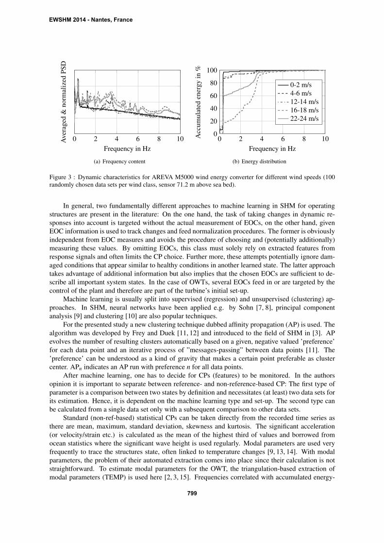
learning and hence accounting for EOC-variations in later SHM steps, Figure 3 shows power spectraldensities (PSD) Sxx(ω) (3(a)) and accumulated energy (AE) levels Exx(ω) (3(b)) for different systemstates using wind speed as a major system variable. Since wind speed drives excitation levels, rotorspeed and in higher regimes the pitch angle, differing frequency contents and energy distributionsappear. It is obvious, that many condition parameters will be influenced by this change in dynamicbehavior. Here, Sxx(ω) is the Fourier transform of the auto-correlated time signal Φxx(τ) for a singlesensor x as

Sxx(ω) = F{Φxx(τ)} (1)

and Exx(ω) as normalized sum of Sxx(ω), with

Exx(ωi) =i

∑n=1

Sxx(ωn) (2)

Exx(ωi) =100∗ Exx(ωi)

Exx(ωi =fs2 )

. (3)

The AE is an indicator for energy distribution within a signal, taking changes in the whole frequencyrange into account instead of tracking single peaks. It was used for instance for shape analysis [4] andto characterize earthquakes in time domain [5]. The mean frequency between 90 and 100% AE-levelsfor single sensors, is used as a CP later on.

2. SHM FOR LARGE SCALE STRUCTURES

Originating from a plausible data base, it is important to clearly distinguish between machine learningprocedures and CPs. Even though these two come closely linked in most cases and a combination ofboth will always be necessary, their task is different. The CP is the monitored value while machinelearning captures a dependency between CP and system states. The close relationship sometimes leadsto confusion. As an illustrating example, Fritzen et al. [6] use CPs from stochastic subspace identifica-tion (SSI) in a sophisticated SHM scheme as goal values not as machine learning technique. Machinelearning is done through a multi dimensional fuzzy classification of temperature measurements.

EWSHM 2014 - Nantes, France

798

0 2 4 6 8 10Frequency in Hz

Ave

rage

d&

norm

aliz

edPS

D

(a) Frequency content

0 2 4 6 8 100

20

40

60

80

100

Frequency in Hz

Acc

umul

ated

ener

gyin

%

0-2 m/s4-6 m/s12-14 m/s16-18 m/s22-24 m/s

(b) Energy distribution

Figure 3 : Dynamic characteristics for AREVA M5000 wind energy converter for different wind speeds (100randomly chosen data sets per wind class, sensor 71.2 m above sea bed).

In general, two fundamentally different approaches to machine learning in SHM for operatingstructures are present in the literature: On the one hand, the task of taking changes in dynamic re-sponses into account is targeted without the actual measurement of EOCs, on the other hand, givenEOC information is used to track changes and feed normalization procedures. The former is obviouslyindependent from EOC measures and avoids the procedure of choosing and (potentially additionally)measuring these values. By omitting EOCs, this class must solely rely on extracted features fromresponse signals and often limits the CP choice. Further more, these attempts potentially ignore dam-aged conditions that appear similar to healthy conditions in another learned state. The latter approachtakes advantage of additional information but also implies that the chosen EOCs are sufficient to de-scribe all important system states. In the case of OWTs, several EOCs feed in or are targeted by thecontrol of the plant and therefore are part of the turbine’s initial set-up.

Machine learning is usually split into supervised (regression) and unsupervised (clustering) ap-proaches. In SHM, neural networks have been applied e.g. by Sohn [7, 8], principal componentanalysis [9] and clustering [10] are also popular techniques.

For the presented study a new clustering technique dubbed affinity propagation (AP) is used. Thealgorithm was developed by Frey and Duek [11, 12] and introduced to the field of SHM in [3]. APevolves the number of resulting clusters automatically based on a given, negative valued ’preference’for each data point and an iterative process of ”messages-passing” between data points [11]. The’preference’ can be understood as a kind of gravity that makes a certain point preferable as clustercenter. APn indicates an AP run with preference n for all data points.

After machine learning, one has to decide for CPs (features) to be monitored. In the authorsopinion it is important to separate between reference- and non-reference-based CP: The first type ofparameter is a comparison between two states by definition and necessitates (at least) two data sets forits estimation. Hence, it is dependent on the machine learning type and set-up. The second type canbe calculated from a single data set only with a subsequent comparison to other data sets.

Standard (non-ref-based) statistical CPs can be taken directly from the recorded time series asthere are mean, maximum, standard deviation, skewness and kurtosis. The significant acceleration(or velocity/strain etc.) is calculated as the mean of the highest third of values and borrowed fromocean statistics where the significant wave height is used regularly. Modal parameters are used veryfrequently to trace the structures state, often linked to temperature changes [9, 13, 14]. With modalparameters, the problem of their automated extraction comes into place since their calculation is notstraightforward. To estimate modal parameters for the OWT, the triangulation-based extraction ofmodal parameters (TEMP) is used here [2, 3, 15]. Frequencies correlated with accumulated energy-

EWSHM 2014 - Nantes, France

799

levels as described in Equation (2) and (3) form new parameters. Complete frequency spectra can alsobe taken as multidimensional parameters [16,17]. Reference-based residues from stochastic subspaceidentification (SSI) [3, 6, 18] or vector autoregressive models (VAR) [3, 19] have also become popularCPs. A selection of these parameters is applied here.

A further important tool for hypothesis testing are so-called control charts where a control vari-able is plotted over time [20]. Upper- and lower control limit (UCL/LCL) indicate value regions for’normal’ behavior, the healthy state or H0-hypothesis in the present case. Kullaa uses different con-trol charts for SHM at a wooden bridge model and a vehicle crane [21]. Here, a standardized residualcontrol chart with varying LCL/UCL is introduced. In the previous steps, every incoming data set wasassigned to a cluster where a parameter distribution is present for each CP-type. These distributionsare not necessarily of known kind and might be non-symmetric. LCL and UCL are defined as 0.1 and99.9% percentiles, respectively. Which leads to the following definition of the control variable zX

i, j as

zXi, j =

CPX

i, j

|CPX , j,ck50 −CP

X , j,ck99.9 |

for CPXi, j > 0

CPXi, j

|CPX , j,ck50 −CP

X , j,ck0.1 |

for CPXi, j < 0

with CPXi, j =CPX

i, j−CPX ,i, j50 . (4)

Where CPX , j,ckn is the n% percentile for CP X in classification j and cluster ck and CPX

i, j is the CP Xestimated for the i-th incoming data set (with respect to classification j), see also Figure 4 and 5. Itshould be emphasized, that, according to the suggested SHM structure, every SHM–proceduresconsists of, and hence can be categorized in, three constituents (even if included passively orunintentionally): Machine Learning – Condition Parameter – Hypothesis Testing.

3. MONITORING THE OWT

The following chapter outlines the application of the introduced SHM scheme to the OWT. It is obvi-ous from Figure 1 that the number of resulting decisions in HT (e.g. through control charts) rapidlyincreases with machine learning types and CPs. Hence, major steps will be displayed through a spe-cific set-up for classification (as ML) in combination with two CPs, namely VAR-residues. Finally,different CPs and classification types are compared by means of false-positive alarms within the con-trol charts. As stated in Section 1., the initial data set is formed from 19,135 sets with 13 EOCsavailable for each set. In the first step, AP is chosen as machine learning algorithm and the data baseis split into a training- (set 1 to 17,119) and testing-phase (set 17,120 to 19,135).

3.1 Training phase

A subset of 2016 randomly chosen sets (2 weeks) is taken from the learning-phase to train the system.One manual classification by wind speed and four AP set-ups, named ’AP1’ to ’AP4’, are executed(see Table 1). The AP uses EOCs normalized to a range of [-1;0] each. All set-ups differ in number andtype of selected EOCs and resulting number of clusters. For classification ’AP2’ Figure 4(a) showsthe EOC distributions for each of the seven resulting clusters. Distributions for each cluster per EOCare combined. AP groups the data sets in this five-dimensional EOC-space very well and each clusterspans different EOC ranges. Each data set is assigned to a single cluster and hence reference-basedCPs can also be calculated.

Since the VAR-residue (CPR2) is a reference-based CP, each data set in a cluster is compared

to a mean reference matrix of the cluster, VAR-parameters in this case. The results can be seenin Figure 4(b) where −(CPR2 − 1) is plotted in logarithmic scale3 and grouped per cluster (1-7).

3CPR2 ∈ [−∞,1]; A value of 1 corresponds to good agreement between reference and current data set. The transformationis done to allow logarithmic scaling. Accordingly, large values indicate bad agreement between reference and actual dataset.

EWSHM 2014 - Nantes, France

800

0

0.5

1

Rot

orsp

d.

Windspd. Nacpos

Tem

p.

Turb

ulen

ce

Nor

mal

ized

EO

C 1234567

(a) EOC distributions in clusters

10−0.5

1 2 3 4 5 6 7

CP

R2in−(C

PR

2−

1)

CPCP50µCPn

(b) CP distributions in clusters

Figure 4 : 4(a) EOC distributions for cluster 1 to 7 in classification ”AP2”. Here, 5/95%, 25/75% and median aremarked by bars, ”+” and ”o”, respectively. 4(b) Corresponding distribution of VAR-residue sorted by clusters.CP given with mean (µ), median (CP50), and percentiles (CPn, n = 5,25,75,95). Distributions for non-clustereddata in very left section.

Clearly, the CPR2has a distinctively different distribution for the different clusters. The distributions

for non-clustered data are indicated in the very left section: The very left marks indicate a distributionwhere each data set is compared to its predecessor, with good results but the draw-back of omittingconsecutive degradation. The right marks in the very left section result from single training cluster.

All other CP are processed accordingly, resulting in CP distributions for each cluster in eachclassification. Note, that non-reference-based CPs are calculated only once, while reference basedCPs need to be re-calculated for each classification set-up since data set assignment to clusters andhence the reference matrices change. The CP-distributions per cluster can now be used to evaluatenew incoming data sets for the testing phase.

3.2 Testing phase

For testing, 2016 successive data sets were chosen from the testing–part of the data base and processed.For validity, the distribution of EOC values during testing was checked against the training phase:Distribution densities differ, but all testing EOC-ranges are covered in the training phase. The testingphase can be carried out for each classification type. In a first step, a new data set is assigned to acluster by minimum normalized EOCs-distances. Afterwards, the CP is calculated and compared tothe CP–distribution learned for the specific cluster (and classification). To draw a control chart asdescribed in 2., the CP is compared to median and 0.1 or 99.9%-percentile (see equation (4)) to rangebetween [-1,1] for acceptance of the H0-hypothesis.

Figure 5 displays such a normalized control chart for CPR2and CPMBox in ’AP2’ with lower and

upper control limits. The control variable is plotted chronologically for all 2016 data sets and out-of-control points (H1-hypothesis) can be detected in 3.22%/0.69% of the data sets. Considering thelimited training period, slightly differing EOCs and the fast return of CPR2

and CPMBox from out-of-control to in-control, the control chart leads to the conclusion, that, with respect to CPR2

and CPMBox,the system remains in a normal state during observation. Taking the percentage of out-of-controlpoints as a first quality index, one can compare the different classifications and CPs. Table 1 showsthe outlier percentage for all five classifications and 8 CPs. Here, standard statistical values (first threeCPs) result in moderate outlier percentages. For these CPs, average values are given for all 24 channelssince the CPs are calculated for each sensor. Further, tracking the first modal frequency results in largeroutlier percentages. Dividing the training data into more clusters to capture the dynamic behavior ineven more detail might resolve this problem. AE, SSI- and VAR-residues show good results for theAP classifications with few outliers. The manual classifications results in a large number of falsealarms. Classifications with more EOCs included tend to perform better. The two outlier percentagesbelonging to the control charts in Fig.5(b) are highlighted.

EWSHM 2014 - Nantes, France

801

0 500 1,000 1,500 2,000

−1

0

1

Outlier 3.22%/0.2%

Data set #

CP-

Nor

mal

ized

:

(a) Control chart: CPR2

0 500 1,000 1,500 2,000

−1

0

1

Outlier 0.69%/0.2%

Data set #

CP-

Nor

mal

ized

:

CP1

UCLLCL

(b) Control chart: CPMBox

Figure 5 : Normalized control charts over a period of two weeks (2016 10 min sets) for two VAR-residues:CPR2

(5(a)) and CPMBox(5(b)). Upper- and lower control limit (UCL/LCL) are marked with red lines.

Table 1 : Percentage of false positive alarms for different CPs and classificationsClassification set-up Manual AP1 AP2 AP3 AP4

Used EOCs2 [1,2] [1,2] [1−5] [1−7,11] [1−13]No. of Clusters 4 13 7 8 11

Skewness (for each channel) 2.2 2.3 1.4 1.6 1.2Kurtosis (for each channel) 2.3 2.9 1.9 1.8 1.5

Significant acceleration (for each channel) 6.3 3.5 1.5 2.1 1.82nd modal frequency 5.7 4.2 7.2 4.7 7.7

Accumulated Energy (90-100% energy level) 10.9 2.5 1.9 2.3 1.8Nullspace based SSI Residue 3.7 1.9 1.1 0.8 0.5

VAR-R2 Residue 77.4 5.7 3.2 2.0 1.1VAR-MBox Residue 23.0 1.8 0.7 1.3 0.8

CONCLUSIONS

It is concluded, that every SHM approach necessitates, consists of, and can be categorized in threemain steps: Condition parameter, machine learning, and hypothesis testing. This leads to a modu-lar SHM-scheme, which was presented and applied to an offshore wind turbine using 10 min datasets recorded over a period of more than one year. Response data from accelerometers along withmeasured environmental and operational conditions, serve as input for the SHM-scheme. Machinelearning, the calculation of condition parameters and hypothesis testing through the estimation ofprobabilistic models for those parameters lead to normalized control charts that can be easily evalu-ated and compared to provide observability. Giving the ability to include different machine learningalgorithms and condition parameters, the scheme is generally applicable to structures in civil and me-chanical engineering. Further, all applied combinations of machine learning and condition parametersresult in false positive alarms from the control charts, which allow a good comparison. The investi-gated 5 MW offshore wind turbine remained in healthy condition throughout training and testing. Dataclassification through Affinity Propagation was used as machine learning technique and different con-dition parameters were implemented. The known healthy conditions are in agreement with the drawncontrol charts, where, with smaller and larger numbers of outliers, the control variable remains withinthe limits without suffering from strong shifts. Other control charts, e.g. with rational subgroups, canbe introduced in future work as desired. Also, further EOC combinations and classification set-upsshould be tested along with additional condition parameters.

EWSHM 2014 - Nantes, France

802

REFERENCES

[1] A. Rytter. Vibration based inspection of civil engineering structures. PhD thesis, Aalborg University,Denmark, 1993.

[2] Moritz W. Hackell and Raimund Rolfes. Monitoring a 5MW offshore wind energy converter—Conditionparameters and triangulation based extraction of modal parameters. Mechanical Systems and SignalProcessing, 40(1):322–343, October 2013.

[3] Moritz W. Hackell and Raimund Rolfes. Long-term monitoring of modal parameters for SHM at a 5MW offshore wind turbine. In Proceedings of the 9th International Workshop on Structural HealthMonitoring, pages 1310–1317, Stanford, CA, USA, 2013. Chang, F.-K. (Ed.), DEStech Publications Inc.

[4] Luciano da Fontoura Da Costa and Roberto Marcondes Cesar. Shape analysis and classification: theoryand practice. Image processing series. CRC Press, Boca Raton, FL, 2001.

[5] Haruo Takizawa and Paul C. Jennings. Collapse of a model for ductile reinforced concrete frames underextreme earthquake motions. Earthquake Engineering & Structural Dynamics, 8(2):117–144, 1980.

[6] Claus-Peter Fritzen and Peter Kraemer. Vibration based damage detection for structures of offshore windenergy plants. In Proceedings of the 8th International Workshop on Structural Health Monitoring, pages1656–1663, Stanford, CA, USA, 2011. Chang, F.-K. (Ed.), DEStech Publications Inc.

[7] H. Sohn, K. Worden, and C. R. Farrar. Statistical damage classification under changing environmentaland operational conditions. Journal of Intelligent Material Systems and Structures, 13(9):561–574,September 2002.

[8] Hoon Sohn, Charles R. Farrar, Norman F. Hunter, and Keith Worden. Structural health monitoring usingstatistical pattern recognition techniques. Journal of Dynamic Systems, Measurement, and Control,123(4):706, 2001.

[9] A. Deraemaeker, E. Reynders, G. De Roeck, and J. Kullaa. Vibration-based structural health moni-toring using output-only measurements under changing environment. Mechanical Systems and SignalProcessing, 22(1):34–56, January 2008.

[10] K. Worden, H. Sohn, and C.R. Farrar. Novelty detection in a changing environment: Regression andinterpolation approaches. Journal of Sound and Vibration, 258(4):741–761, December 2002.

[11] B. J. Frey and D. Dueck. Clustering by passing messages between data points. Science, 315(5814):972–976, February 2007.

[12] Delbert Dueck. Affinity Propagation: Clustering Data by Passing Messages. PhD thesis, University ofToronto, Graduate Department of Electrical & Computer Engineering, 2009.

[13] Hoon Sohn, Mark Dzwonczyk, Erik G. Straser, Anne S. Kiremidjian, Kincho H. Law, and Teresa Meng.An experimental study of temperature effect on modal parameters of the alamosa canyon bridge. In ofthe Alamosa Canyon Bridge.” Earthquake Eng. and Structural Dynamics, page 879–897. John Wiley &Sons, 1999.

[14] Chengyin Liu and John T. DeWolf. Effect of temperature on modal variability of a curved concretebridge under ambient loads. Journal of Structural Engineering, 133(12):1742–1751, December 2007.

[15] Yilan Zhang, Moritz W. Hackell, Jerome Peter Lynch, and Raimund Rolfes. Automated modal pa-rameter extraction and statistical analysis of the new carquinez bridge response to ambient excitations.In Proceedings of the 32nd International Modal Analysis Conference (IMAC), Orlando, Florida, USA,2014.

[16] Spilios D. Fassois and John S. Sakellariou. Statistical time series methods for SHM. In Christian Boller,Fu-Kuo Chang, and Yozo Fujino, editors, Encyclopedia of Structural Health Monitoring. John Wiley &Sons, Ltd, Chichester, UK, September 2009.

[17] Cecilia Surace and Keith Worden. Novelty detection in a changing environment: A negative selectionapproach. Mechanical Systems and Signal Processing, 24(4):1114–1128, May 2010.

[18] Michael Dohler, Laurent Mevel, and Falk Hille. Subspace-based damage detection under changes in theambient excitation statistics. Mechanical Systems and Signal Processing, 45(1):207–224, March 2014.

[19] John Neter, William Wasserman, Michael H Kutner, et al. Applied linear statistical models, volume 4.Irwin Chicago, 1996.

[20] Douglas C Montgomery. Introduction to statistical quality control. Wiley, Hoboken, 5 edition, 2005.[21] Jyrki Kullaa. Distinguishing between sensor fault, structural damage, and environmental or operational

effects in structural health monitoring. Mechanical Systems and Signal Processing, 25(8):2976–2989,November 2011.

EWSHM 2014 - Nantes, France

803