a mosaic sampler - calvin collegerpruim/talks/rminis/mosaicsampler.pdfintro using formulas xtras...
TRANSCRIPT

Intro Using Formulas Xtras do()ing stuff Calculus Team
A mosaic Sampler
Randall Pruim, Calvin College
JMM 2013
Intro Using Formulas Xtras do()ing stuff Calculus Team
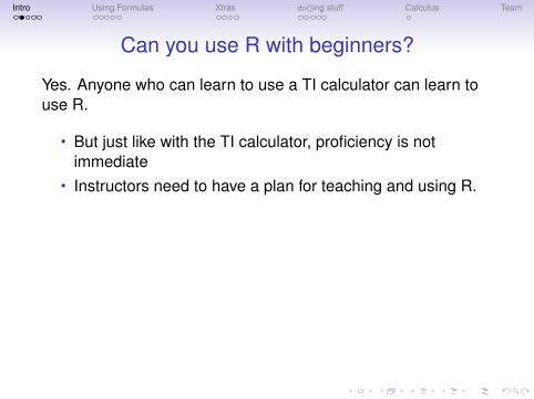
Can you use R with beginners?
Yes. Anyone who can learn to use a TI calculator can learn touse R.
• But just like with the TI calculator, proficiency is notimmediate
• Instructors need to have a plan for teaching and using R.
Students who have trouble with R usually have other problems.
• R reveals more problems than it causes.• Diagnostic (and teaching) questions:
• What do you want the computer to do?• What does it need to know to do that?
Intro Using Formulas Xtras do()ing stuff Calculus Team
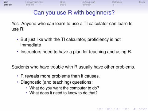
Can you use R with beginners?
Yes. Anyone who can learn to use a TI calculator can learn touse R.
• But just like with the TI calculator, proficiency is notimmediate
• Instructors need to have a plan for teaching and using R.
Students who have trouble with R usually have other problems.
• R reveals more problems than it causes.• Diagnostic (and teaching) questions:
• What do you want the computer to do?• What does it need to know to do that?

Intro Using Formulas Xtras do()ing stuff Calculus Team
Less Volume, More Creativity
“A lot of times you end up putting in a lot more volume,because you are teaching fundamentals and you areteaching concepts that you need to put in, but you maynot necessarily use because they are building blocksfor other concepts and variations that will come off ofthat . . . In the offsea- son you have a chance to takea step back and tailor it more specifically towards yourteam and towards your players.”
– Mike McCarthy, Head Coach, Green Bay Packers
“Perfection is achieved, not when there is nothingmore to add, but when there is nothing left to takeaway.”
– Antoine de Saint-Exupery
Intro Using Formulas Xtras do()ing stuff Calculus Team
Less Volume, More Creativity“A lot of times you end up putting in a lot more volume,because you are teaching fundamentals and you areteaching concepts that you need to put in, but you maynot necessarily use because they are building blocksfor other concepts and variations that will come off ofthat . . . In the offsea- son you have a chance to takea step back and tailor it more specifically towards yourteam and towards your players.”
– Mike McCarthy, Head Coach, Green Bay Packers
“Perfection is achieved, not when there is nothingmore to add, but when there is nothing left to takeaway.”
– Antoine de Saint-Exupery
Intro Using Formulas Xtras do()ing stuff Calculus Team
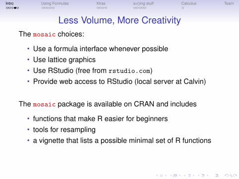
Less Volume, More CreativityThe mosaic choices:
• Use a formula interface whenever possible• Use lattice graphics• Use RStudio (free from rstudio.com)• Provide web access to RStudio (local server at Calvin)
The mosaic package is available on CRAN and includes
• functions that make R easier for beginners• tools for resampling• a vignette that lists a possible minimal set of R functions
Intro Using Formulas Xtras do()ing stuff Calculus Team
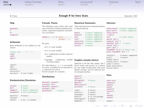
R. Pruim Enough R for Intro Stats September, 2012
Help
apropos()
?
??
example()
Arithmetic
Basic arithmetic is very similar to a cal-culator.
# basic ops: + - * / ^ ( )
log()
exp()
sqrt()
log10()
abs()
choose()
factorial()
uniroot() # root finder
Randomization/Simulation
rflip() # mosaic
do() # mosaic
sample() # mosaic augmented
resample() # with replacement
shuffle() # mosaic
rbinom()
rnorm() # etc, if needed
Formula Theme
The following syntax (often with someparts omitted) is used for graphical sum-maries, numerical summaries, and infer-ence procedures.
fname( y ~ x | z, data=...,
groups=... )
For plots
• y: is y-axis variable
• x: is x-axis variable
• z: conditioning variable (separatepanels)
• groups: conditioning variable(overlaid graphs)
For other things y ~ x | z can usuallybe read y is modeled by (or depends on)x separately for each z .See the sampler for examples.
Distributions
pbinom(); pnorm();
pchisq(); pt()
qbinom(); qnorm();
qchisq(); qt()
plotDist(); # mosaic
Numerical Summaries
These functions have a formula interfaceto match plotting.
mean() # mosaic augmented
median() # mosaic augmented
sd() # mosaic augmented
var() # mosaic augmented
quantile() # mosaic augmented
favstats() # mosaic
tally() # mosaic
Graphics (mostly lattice)
lattice is not the only option, but Ifind it works well because (a) it allowsfor easy multi-variable plots with gooddefault settings, and (b) lattice usesthe formula interface.
bwplot()
xyplot()
histogram() # mosaic
qqmath()
densityplot()
plotFun() # mosaic
ladd() # mosaic
dotPlot() # mosaic
bargraph() # mosaic
mosaic() # in vcd package
xhistogram() # mosaic
xqqmath() # mosaic
Inference
binom.test() # mosaic augmented
prop.test() # mosaic augmented
chisq.test()
t.test()
lm() # linear models
anova( lm() )
summary( lm() )
makeFun( lm() ) # mosaic
resid( lm() )
plot( lm() )
TukeyHSD( lm () ) # mosaic aug
plot( TukeyHSD( lm() ) )
confint() # mosaic augmented
pval() # mosaic
fisher.test()
xchisq.test() # mosaic
power.t.test()
power.prop.test()
wilcox.test()
Data
read.csv()
summary()
names()
head()
subset()
factor()
c()
cbind()
rbind()
merge()
Intro Using Formulas Xtras do()ing stuff Calculus Team
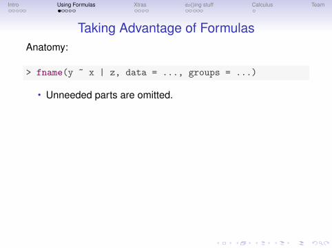
Taking Advantage of FormulasAnatomy:
> fname(y ~ x | z, data = ..., groups = ...)
• Unneeded parts are omitted.
Physiology: y depends on x, conditioned on z
• Plots:• y along vertical axis• x along horizontal axis• z divides plot into subplots (panels)• groups used to overlay subsets with different colors/shapes
• Numerical summaries augmented to handle formulas• Linear Models can generally be fit by replacing a plotting
function with lm().
Intro Using Formulas Xtras do()ing stuff Calculus Team
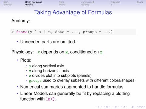
Taking Advantage of FormulasAnatomy:
> fname(y ~ x | z, data = ..., groups = ...)
• Unneeded parts are omitted.
Physiology: y depends on x, conditioned on z
• Plots:• y along vertical axis• x along horizontal axis• z divides plot into subplots (panels)• groups used to overlay subsets with different colors/shapes
• Numerical summaries augmented to handle formulas• Linear Models can generally be fit by replacing a plotting
function with lm().

Intro Using Formulas Xtras do()ing stuff Calculus Team
Taking Advantage of Formulas: tally()
> tally(substance ~ sex,
+ data=HELPrct)
sex
substance female male
alcohol 0.336 0.408
cocaine 0.383 0.321
heroin 0.280 0.272
Total 1.000 1.000
> tally(~ substance & sex,
+ data=HELPrct)
sex
substance female male Total
alcohol 36 141 177
cocaine 41 111 152
heroin 30 94 124
Total 107 346 453

Intro Using Formulas Xtras do()ing stuff Calculus Team
Taking Advantage of Formulas: Numerical Summaries
> mean(age ~ sex, data = HELPrct)
female male
36.3 35.5
> sd(age ~ sex | homeless, data = HELPrct)
female.homeless male.homeless female.housed
6.66 8.61 8.13
male.housed homeless housed
6.71 8.26 7.17
Also works for var(), median(), max(), min(), IQR(), sum(),prop(), count()
Intro Using Formulas Xtras do()ing stuff Calculus Team
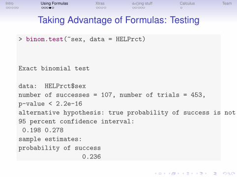
Taking Advantage of Formulas: Testing
> binom.test(~sex, data = HELPrct)
Exact binomial test
data: HELPrct$sex
number of successes = 107, number of trials = 453,
p-value < 2.2e-16
alternative hypothesis: true probability of success is not equal to 0.5
95 percent confidence interval:
0.198 0.278
sample estimates:
probability of success
0.236

Intro Using Formulas Xtras do()ing stuff Calculus Team
Just the Facts Ma’amR’s output can sometimes be overly verbose for beginners.
> interval(t.test(age ~ sex, data = HELPrct))
mean in group female mean in group male
36.25 35.47
lower upper
-0.88 2.45
level
0.95
> pval(t.test(age ~ sex, data = HELPrct))
p.value
0.354
(Remember this p-value for later.)
Intro Using Formulas Xtras do()ing stuff Calculus Team
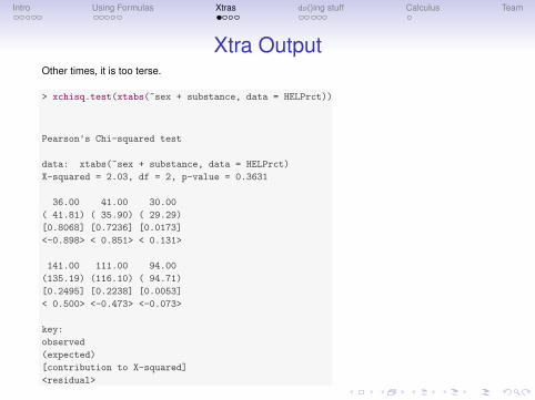
Xtra OutputOther times, it is too terse.
> xchisq.test(xtabs(~sex + substance, data = HELPrct))
Pearson's Chi-squared test
data: xtabs(~sex + substance, data = HELPrct)
X-squared = 2.03, df = 2, p-value = 0.3631
36.00 41.00 30.00
( 41.81) ( 35.90) ( 29.29)
[0.8068] [0.7236] [0.0173]
<-0.898> < 0.851> < 0.131>
141.00 111.00 94.00
(135.19) (116.10) ( 94.71)
[0.2495] [0.2238] [0.0053]
< 0.500> <-0.473> <-0.073>
key:
observed
(expected)
[contribution to X-squared]
<residual>

Intro Using Formulas Xtras do()ing stuff Calculus Team
Xtra Graphics
> xhistogram( ~age , data=HELPrct, fit='normal',+ width=5, groups = age > 30)
age
Den
sity
0.00
0.01
0.02
0.03
0.04
0.05
20 30 40 50 60
Other features:
• Easy horizontal and vertical reference lines.

Intro Using Formulas Xtras do()ing stuff Calculus Team
More Xtras> xpnorm(10, mean = 8, sd = 1.23)
If X ~ N(8,1.23), then
P(X <= 10) = P(Z <= 1.626) = 0.948
P(X > 10) = P(Z > 1.626) = 0.052
[1] 0.948
dens
ity
0.1
0.2
0.3
0.4
4 6 8 10 12
10(z=1.626)
0.948 0.052

Intro Using Formulas Xtras do()ing stuff Calculus Team
More Xtras> require(fastR)> model <- lm(time ~ sqrt(height), data = balldrop)> fit <- makeFun(model)> xyplot(time ~ height, data = balldrop)> plotFun(fit(height) ~ height, add = TRUE)
height
time
0.25
0.30
0.35
0.40
0.45
0.50
0.4 0.6 0.8 1.0 1.2
●●●●●
●●●●●
●●●●●
●●●●●
●●●●●
●●●●●
Intro Using Formulas Xtras do()ing stuff Calculus Team
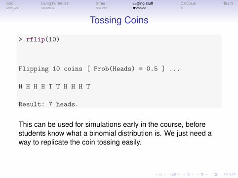
Tossing Coins
> rflip(10)
Flipping 10 coins [ Prob(Heads) = 0.5 ] ...
H H H H T T H H H T
Result: 7 heads.
This can be used for simulations early in the course, beforestudents know what a binomial distribution is. We just need away to replicate the coin tossing easily.
Intro Using Formulas Xtras do()ing stuff Calculus Team
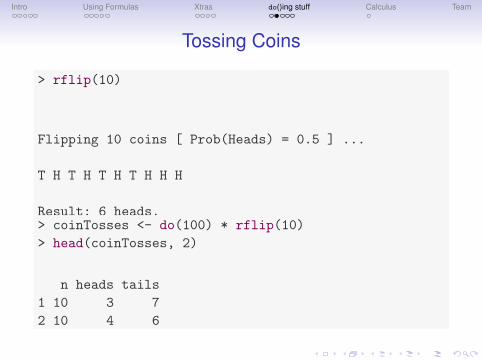
Tossing Coins
> rflip(10)
Flipping 10 coins [ Prob(Heads) = 0.5 ] ...
T H T H T H T H H H
Result: 6 heads.> coinTosses <- do(100) * rflip(10)
> head(coinTosses, 2)
n heads tails
1 10 3 7
2 10 4 6

Intro Using Formulas Xtras do()ing stuff Calculus Team
Additional Plots
> mybreaks <- 0.5 + (-1:10)> dotPlot(~heads, data = coinTosses, breaks = mybreaks)> freqpolygon(~heads, data = coinTosses, breaks = mybreaks)
heads
Cou
nt
0
5
10
15
20
25
0 2 4 6 8 10
●●●
●●●●●●●●●●●●
●●●●●●●●●●●●●●●●●●●●
●●●●●●●●●●●●●●●●●●●●●●●●●●●
●●●●●●●●●●●●●●●●●●●●●●
●●●●●●●●●●
●●●●
●●
heads
Per
cent
of T
otal
0
5
10
15
20
25
0 2 4 6 8 10
● ●● ●● ●●●●● ●● ● ●●● ●● ●● ●●●●●●● ●● ●●● ●●● ●● ●● ●● ●● ● ● ●●●● ● ●● ●● ●● ● ●● ●●● ● ●●● ●●● ●● ●● ●●● ●● ●● ●● ● ●●●● ●●●● ●●● ● ●●● ●●

Intro Using Formulas Xtras do()ing stuff Calculus Team
do()ing the mosiac shuffle()
> do(1) * lm(age ~ sex, HELPrct)
Intercept sexmale sigma r.squared1 36.3 -0.784 7.71 0.00187
> null.dist <- do(1000) * lm(age ~ shuffle(sex), HELPrct)> head(null.dist, 1)
Intercept sexmale sigma r.squared1 36 -0.405 7.72 0.000498
> with(null.dist, tally(abs(sexmale) >= 0.784), format = "prop")
TRUE FALSE Total342 658 1000
Intro Using Formulas Xtras do()ing stuff Calculus Team
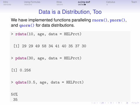
Data is a Distribution, TooWe have implemented functions paralleling rnorm(), pnorm(),and qnorm() for data distributions.
> rdata(10, age, data = HELPrct)
[1] 29 29 49 58 34 41 40 35 37 30
> pdata(30, age, data = HELPrct)
[1] 0.256
> qdata(0.5, age, data = HELPrct)
50%
35

Intro Using Formulas Xtras do()ing stuff Calculus Team
CalculusDifferentiation:
> f <- D(A * sin(x + B) ~ x, A = 1, B = 0)
> f(pi)
[1] -1
> f(pi, A = 3, B = pi)
[1] 3
> randx <- runif(4, -pi, pi)
> f(randx) - cos(randx)
[1] 0 0 0 0
Anti-differentiation:
> F <- antiD(dnorm(x) ~ x)> # F(0) == 0 by default> F(randx) - pnorm(randx)
[1] -0.5 -0.5 -0.5 -0.5
> # Using G(-Inf) == 0 gives pdf> G <- antiD(dnorm(x) ~ x, from = -Inf)
> G(randx) - pnorm(randx)
[1] -0.5 -0.5 -0.5 -0.5
> G(2)
[1] 0.477
Intro Using Formulas Xtras do()ing stuff Calculus Team
The mosaic team
R Pruim D Kaplan N Horton YouCalvin C Macalaster C Smith C
http://www.mosaic-web.org

Intro Using Formulas Xtras do()ing stuff Calculus Team
The mosaic team
R Pruim D Kaplan N Horton YouCalvin C Macalaster C Smith C
http://www.mosaic-web.org