a moving-barber-pole illusion - uci social...

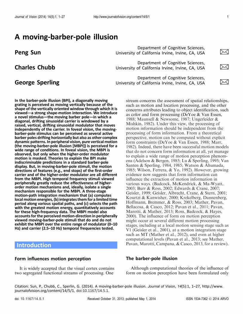
A moving-barber-pole illusion

Peng Sun $Department of Cognitive Sciences,

University of California Irvine, Irvine, CA, USA

Charles Chubb $Department of Cognitive Sciences,


George Sperling $Department of Cognitive Sciences,


In the barber-pole illusion (BPI), a diagonally movinggrating is perceived as moving vertically because of theshape of the vertically oriented window through which it isviewed—a strong shape-motion interaction. We introducea novel stimulus—the moving barber pole—in which adiagonal, drifting sinusoidal carrier is windowed by araised, vertical, drifting sinusoidal modulator that movesindependently of the carrier. In foveal vision, the moving-barber-pole stimulus can be perceived as several activebarber poles drifting horizontally but also as other complexdynamic patterns. In peripheral vision, pure verticalmotion(the moving-barber-pole illusion [MBPI]) is perceived for awide range of conditions. In foveal vision, the MBPI isobserved, but only when the higher-order modulatormotion is masked. Theories to explain the BPI makeindiscriminable predictions in a standard barber-poledisplay. But, in moving-barber-pole stimuli, the motiondirections of features (e.g., end stops) of the first-ordercarrier and of the higher-order modulator are all differentfrom the MBPI. High temporal frequency stimuli viewedperipherally greatly reduce the effectiveness of higher-order motion mechanisms and, ideally, isolate a singlemechanism responsible for the MBPI. A three-stagemotion-path integration mechanism that (a) computeslocalmotion energies, (b) integrates them fora limited timeperiod along various spatial paths, and (c) selects the pathwith the greatest motion energy, quantitatively accountsfor these high-frequency data. The MBPI model alsoaccounts for the perceivedmotion-direction in peripherallyviewed moving-barber-pole stimuli that do and do notexhibit the MBPI over the entire range of modulator (0–10Hz) and carrier (2.5–10 Hz) temporal frequencies tested.

Introduction

Form influences motion perception

It is widely accepted that the visual cortex containstwo segregated functional streams of processing. One

stream concerns the assessment of spatial relationships,such as motion and location processing, and the otherconcerns attributes leading to object identification, suchas color and form processing (DeYoe & Van Essen,1988; Maunsell & Newsome, 1987; Ungerleider &Mishkin, 1982). Under this view, the processing ofmotion information should be independent from theprocessing of form information. From a theoreticalperspective, motion can be computed without explicitform constraints (DeYoe & Van Essen, 1988; Marr,1982). Indeed, there have been successful motion modelsthat do not concern form information at all, yet manageto explain a wide range of motion perception phenom-ena (Adelson & Bergen, 1985; Lu & Sperling, 1995; VanSanten & Sperling, 1984, 1985; Watson & Ahumada,1985; Wilson, Ferrera, & Yo, 1992). However, growingevidence now suggests that form information caninfluence the extraction of motion information invarious ways. (Badcock, McKendrick, & Ma-Wyatt,2003; Burr & Ross, 2002; Edwards & Crane, 2007;Geisler, 1999; Geisler, Albrecht, Crane, & Stern, 2001;Kourtzi & Kanwisher, 2000; Krekelberg, Dannenberg,Hoffmann, Bremmer, & Ross, 2003; Mather, Pavan,Bellacosa, & Casco, 2012; Pavan et al., 2011; Pavan,Marotti, & Mather, 2013; Ross, Badcock, & Hayes,2000). The influence of form on motion perceptionmight occur at several different motion processingstages, including at a local motion sensing stage such asV1 (Geisler et al., 2001), at a motion integration stagesuch as MT (Mather et al., 2012), and even at highercomputational levels (Pavan et al., 2013; see Mather,Pavan, Marotti, Campana, & Casco, 2013, for a review).

The barber-pole illusion

Although computational theories of the influence ofform on motion perception have been formulated only

Citation: Sun, P., Chubb, C., Sperlin, G. (2014). A moving-barber-pole illusion. Journal of Vision, 14(5):1, 1–27, http://www.journalofvision.org/content/14/5/1, doi:10.1167/14.5.1.

Journal of Vision (2014) 14(5):1, 1–27 1http://www.journalofvision.org/content/14/5/1

doi: 10 .1167 /14 .5 .1 ISSN 1534-7362 � 2014 ARVOReceived October 31, 2013; published May 1, 2014

mailto:[email protected]






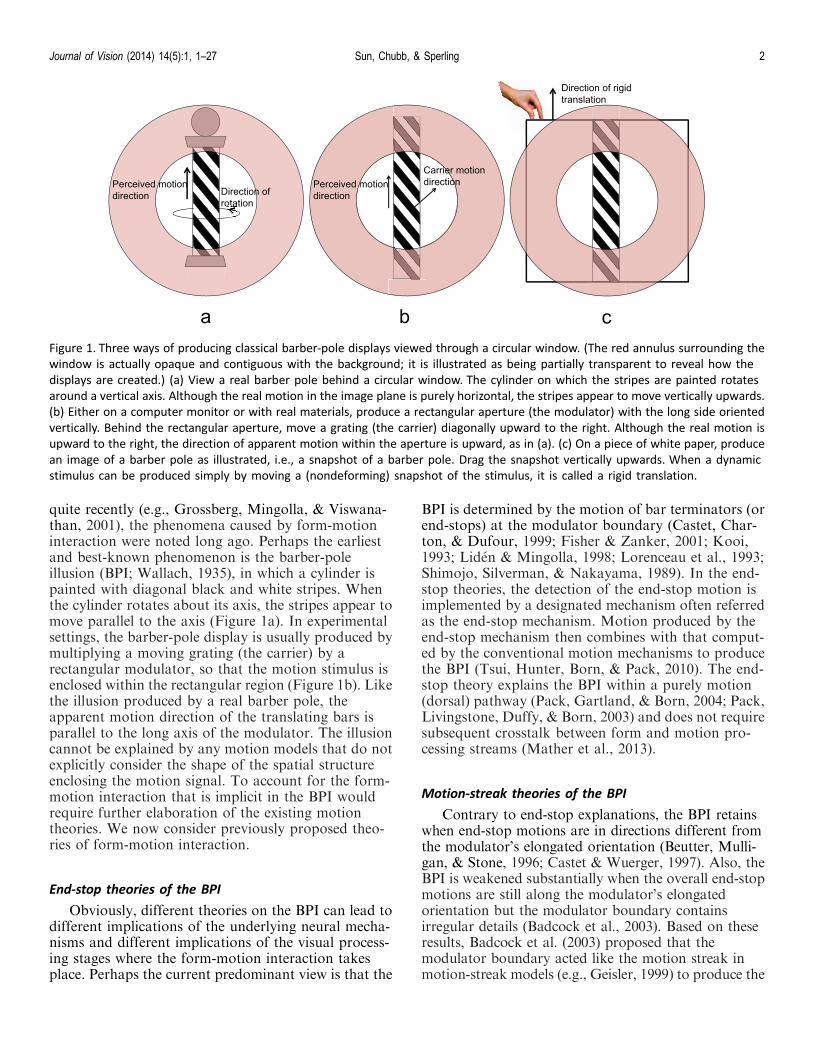
quite recently (e.g., Grossberg, Mingolla, & Viswana-than, 2001), the phenomena caused by form-motioninteraction were noted long ago. Perhaps the earliestand best-known phenomenon is the barber-poleillusion (BPI; Wallach, 1935), in which a cylinder ispainted with diagonal black and white stripes. Whenthe cylinder rotates about its axis, the stripes appear tomove parallel to the axis (Figure 1a). In experimentalsettings, the barber-pole display is usually produced bymultiplying a moving grating (the carrier) by arectangular modulator, so that the motion stimulus isenclosed within the rectangular region (Figure 1b). Likethe illusion produced by a real barber pole, theapparent motion direction of the translating bars isparallel to the long axis of the modulator. The illusioncannot be explained by any motion models that do notexplicitly consider the shape of the spatial structureenclosing the motion signal. To account for the form-motion interaction that is implicit in the BPI wouldrequire further elaboration of the existing motiontheories. We now consider previously proposed theo-ries of form-motion interaction.

End-stop theories of the BPI

Obviously, different theories on the BPI can lead todifferent implications of the underlying neural mecha-nisms and different implications of the visual process-ing stages where the form-motion interaction takesplace. Perhaps the current predominant view is that the

BPI is determined by the motion of bar terminators (orend-stops) at the modulator boundary (Castet, Char-ton, & Dufour, 1999; Fisher & Zanker, 2001; Kooi,1993; Liden & Mingolla, 1998; Lorenceau et al., 1993;Shimojo, Silverman, & Nakayama, 1989). In the end-stop theories, the detection of the end-stop motion isimplemented by a designated mechanism often referredas the end-stop mechanism. Motion produced by theend-stop mechanism then combines with that comput-ed by the conventional motion mechanisms to producethe BPI (Tsui, Hunter, Born, & Pack, 2010). The end-stop theory explains the BPI within a purely motion(dorsal) pathway (Pack, Gartland, & Born, 2004; Pack,Livingstone, Duffy, & Born, 2003) and does not requiresubsequent crosstalk between form and motion pro-cessing streams (Mather et al., 2013).

Motion-streak theories of the BPI

Contrary to end-stop explanations, the BPI retainswhen end-stop motions are in directions different fromthe modulator’s elongated orientation (Beutter, Mulli-gan, & Stone, 1996; Castet & Wuerger, 1997). Also, theBPI is weakened substantially when the overall end-stopmotions are still along the modulator’s elongatedorientation but the modulator boundary containsirregular details (Badcock et al., 2003). Based on theseresults, Badcock et al. (2003) proposed that themodulator boundary acted like the motion streak inmotion-streak models (e.g., Geisler, 1999) to produce the

Figure 1. Three ways of producing classical barber-pole displays viewed through a circular window. (The red annulus surrounding the

window is actually opaque and contiguous with the background; it is illustrated as being partially transparent to reveal how the

displays are created.) (a) View a real barber pole behind a circular window. The cylinder on which the stripes are painted rotates

around a vertical axis. Although the real motion in the image plane is purely horizontal, the stripes appear to move vertically upwards.

(b) Either on a computer monitor or with real materials, produce a rectangular aperture (the modulator) with the long side oriented

vertically. Behind the rectangular aperture, move a grating (the carrier) diagonally upward to the right. Although the real motion is

upward to the right, the direction of apparent motion within the aperture is upward, as in (a). (c) On a piece of white paper, produce

an image of a barber pole as illustrated, i.e., a snapshot of a barber pole. Drag the snapshot vertically upwards. When a dynamic

stimulus can be produced simply by moving a (nondeforming) snapshot of the stimulus, it is called a rigid translation.

Journal of Vision (2014) 14(5):1, 1–27 Sun, Chubb, & Sperling 2

BPI. Badcock et al.’s proposal implied late interactionsbetween the form and motion processing streams.Currently, this theory is heuristic, not computational.

Feature-tracking theories of the BPI

A relatively easy but often implicitly articulatedtheory of the BPI is a feature-tracking theory. Marshall(1990) explained the BPI in a way that is equivalent totracking the two-dimensional (2-D) spatial features—the bar segments—in Figure 1b. Computationally, thefeature-tracking theory is similar to the end-stop theoryinsofar as end-stops are considered as features.

BPI: An implicit computation of the direction of rigidtranslation?

The computation of rigid direction is anotherpossible candidate theory for the BPI. We define ‘‘rigiddirection’’ as follows. Consider a visual stimulus that ispainted or photographed on a sheet of paper; the sheetof paper is translated in a particular direction, thenviewed through a window. The direction in which thepaper moves is the rigid direction of the visual stimulus.A dynamic display has a rigid direction if and only if allits features move in precisely the same direction atprecisely the same speed. The common direction of all

the features is the rigid direction of the dynamic pattern.Obviously, only a tiny subset of dynamic patterns has aunique rigid direction. A barber-pole stimulus like theone shown in Figure 1b viewed through a circularwindow produces exactly the same dynamic stimulus asis produced by dragging a snapshot of the same stimulusupward behind the circular window (Figure 1c). That is,the rigid direction of a barber-pole stimulus is the sameas the modulator’s elongated orientation, as long as themodulator extends beyond the circular aperture.

A number of different algorithms have been pro-posed to extract the rigid direction of a moving image.Therefore, motion models with the components thatimplement these algorithms (Adelson & Movshon,1982; Heeger, 1987; Perrone, 2004, 2012; Simoncelli &Heeger, 1998) can potentially account for the BPI.These models do not require an end-stop processingmechanism or a feature-tracking mechanism.

The moving-barber-pole display

Is the BPI a result of computing a rigid-motiondirection? Or a computation involving tracking featuressuch as end-stops? Or a form-motion interaction thatrequires late crosstalk between the motion and formprocessing pathways? It is difficult to discriminatebetween these theories because for a typical barber-poledisplay, the feature direction, the rigid direction, andthe modulator’s elongated orientation are the same,and all are consistent with the direction of the BPI.

A cartoon illustration

Because the different theories of the BPI all makeidentical motion predictions in a simple barber-poledisplay, we propose a new diagnostic display: movingbarber poles. A typical barber-pole display contains astatic modulator window. In a moving-barber-poledisplay, the modulator moves in a direction and with aspeed that is independent of the carrier motion. Toillustrate this new display, consider three active barberpolesbeing carriedbya truck that is driving leftwardwhilethe barber poles it is carrying are just as active as theynormally are (Figure 2a). Figure 2b illustrates a counter-intuitive fact: When viewed through a circular window, aview identical to the view of the barber poles being carriedby the truck could have been produced by translating asnapshot of the barber poles in a particular direction (i.e.,the direction of rigid translation) that depends on therelative speed of the truck and of the barber-pole stripes.

Constructing the moving-barber-pole stimulus

Figure 2 illustrates the basis of the moving-barber-pole stimuli. In the experiments, the moving-barber-

Figure 2. Cartoon illustration of the moving-barber-pole display.

(a) A realistic scenario in which a moving truck carries three

active barber poles. The truck and the carrier gratings inside

each pole move independently. In this cartoon illustration, the

truck moves horizontally to the left (the modulator) and the

gratings within the barber poles (the carrier) translate

diagonally up to the right. Therefore, motion of the bar

terminators or end-stop motion is up to the left. Although the

stimuli in the experiments are generated as the product of a

modulator sinewave grating and a carrier sinewave grating

viewed through a Gaussian window, they appear very much as

the barber poles on moving truck would appear. (b) Remarkably,

a stimulus identical to (a) can be produced by moving a

snapshot of the barber poles in a particular direction, the

direction of rigid translation, which depends on the speed and

direction of the modulator and of the carrier.


pole display is generated by multiplying a movingsinusoidal grating (carrier) with a raised cosine function(modulator) that moves independently of the carrier.Figure 3a shows a snapshot of a moving-barber-polestimulus. In this example, the carrier moves diagonallyup to the right and the modulator moves horizontallyto the left. The rigid direction is not in line with themodulator’s elongated orientation. By definition, fea-tures move in the direction of rigid translation.Therefore, the direction of the feature motion (i.e., themotion of a bar segment as a whole, or end-stopmotion) is also different from the modulator’s elon-gated orientation. That the elongation motion directionand the rigid motion direction are quite different makesthe moving-barber-pole display highly diagnostic.

Figure 3b through f illustrate the construction of themoving-barber-pole stimulus. Let xc and xm be thespatial frequencies of the carrier and modulatorrespectively, let xtc and xtm be the temporal frequencies

of the carrier and modulator respectively, and let hc andhm be the angles of the two gratings relative to the

vertical, upward direction. Then a moving-barber-pole

stimulus is generated by the following equation:

Sðx; y; tÞ ¼ sinðxcðx cos hc � y sin hcÞ þ xtctÞð1þ cosðxmðx cos hm � y sin hmÞ þ xtmtÞÞ

¼ sinðxcðx cos hc � y sin hcÞ þ xtctÞ

þ 1

2sinðxðxc cos hc þ xm cos hmÞ

� yðxc sin hc þ xm sin hmÞþ ðxtc þ xtmÞtÞ

þ 1

2sinðxðxc cos hc � xm cos hmÞ

� yðxc sin hc � xm sin hmÞþ ðxtc � xtmÞtÞ

ð1Þ

Figure 3. Stimulus decomposition. (a) Snapshot of a moving-barber-pole stimulus. The direction of motion of 2-D spatial features such

as end-stops is, by definition, the same direction as the rigid motion of the image within the circular (Gaussian) window. This

particular stimulus was constructed by multiplying (b) a moving sinusoid carrier with (c) a moving raised cosine modulator. The

multiplication is equivalent to the addition of (d) the carrier grating (same as [b]) and the two side-band components (e). (f). The

length of the arrows is arbitrary; arrows merely indicate directions of motion.


Equation 1 shows that the stimulus can be decom-posed into three Fourier components: the originalcarrier component and two side-band components athalf of the carrier contrast. Knowing the Fouriercomponents allows one to examine the role of the first-order motion system, which is often assumed to computea weighted sum of all available Fourier components.

Introducing the modulator motion adds complica-tions. In particular, the movement of the modulatoritself is a higher-order motion signal. In an attempt toisolate a single or smaller number of mechanisms, theobservations in this study were primarily peripheral,because peripheral viewing involves fewer higher-ordermotion computations (Chubb & Sperling, 1989; Lu &Sperling, 1999).

We used multiple barber poles (versus a single barberpole) so that the center of gravity of all the visiblematerial in the viewing window would remain approx-imately constant and independent of temporal andspatial frequencies of the carrier and modulator.Preliminary observations indicated that some observerswere sensitive to the overall movement of a singlebarber pole. The lateral movement of a single barberpole apparently engages a motion mechanism differentfrom the mechanism that detects movement of thebarber-pole stripes (the carrier). The multiple barber-pole stimulus represents our attempt to reduce thenumber of motion mechanisms involved and thereby,hopefully, to isolate a single motion mechanism.

General methods, all experiments

Apparatus

The experiment was controlled by a Macintosh Intelcomputer running Matlab (MathWorks, Natick, MA)with the Psychtoolbox package (Brainard, 1997).Stimuli were displayed on a 15-in. Mitsubishi Diamand

Pro 710S VGA monitor (Mitsubishi Electric, Tokyo,Japan) with 1024 · 768 resolution running at 85 Hzrefresh rate. A lookup table containing 256 gray levelswas generated by a standard calibration procedure. Themean luminance of all the stimuli was set at 76.7 cd/m2.

Subjects

Three naive subjects and one author (S2), ages 22–29, participated in the experiments. Two of the naivesubjects (S1 and S4) were psychology undergraduatesunassociated with the lab and were kept naive to thepurpose of the experiment. A student from a differentdepartment was the other naive subject (S3). Allmethods were approved by the University of CaliforniaIrvine Institutional Review Board.

Procedure

Peripheral viewing

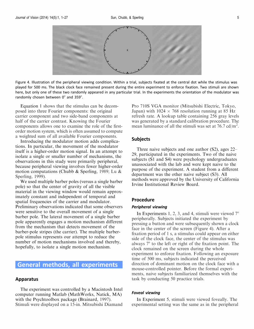
In Experiments 1, 2, 3, and 4, stimuli were viewed 78peripherally. Subjects initiated the experiment bypressing a button and were subsequently shown a clockface in the center of the screen (Figure 4). After afixation period of 1 s, a stimulus could appear on eitherside of the clock face, the center of the stimulus wasalways 78 to the left or right of the fixation point. Theclock remained on the screen during the wholeexperiment to enforce fixation. Following an exposuretime of 500 ms, subjects indicated the perceiveddirection of dominant motion on the clock face with amouse-controlled pointer. Before the formal experi-ments, naive subjects familiarized themselves with thetask by conducting 50 practice trials.

Foveal viewing

In Experiment 5, stimuli were viewed foveally. Theexperimental setting was the same as in the peripheral

Figure 4. Illustration of the peripheral viewing condition. Within a trial, subjects fixated at the central dot while the stimulus was

played for 500 ms. The black clock face remained present during the entire experiment to enforce fixation. Two stimuli are shown

here, but only one of these two randomly appeared in any particular trial. In the experiments the orientation of the modulator was

randomly chosen between 08 and 3598.


viewing condition except that the stimuli appeared inthe center of the monitor.

Experiment 1: Baseline peripheralconditions

The first experiment aimed to establish the baselineperformance for peripherally viewed moving barberpoles with different modulator temporal frequencies.The orientation of the aperture window remainedconstant. The carrier temporal frequency was fixed at10 Hz and the modulator varied. As it did, so did thefeature and rigid motion directions. Insofar as theperceived motion directions were in line with themodulator orientation (and remained so irrespective ofthe variation of the rigid direction with modulatorfrequency), then this form-motion interaction could notbe entirely due to the perceptual computation of therigid (or feature) motion directions.

Stimuli

Stimuli contained a 10 Hz moving sinusoidal grating(carrier) whose contrast was modulated by a raisedcosine function (modulator) that was either static ormoving at variable temporal frequencies. When theangle between the carrier’s and modulator’s motiondirections was greater than p/2, we say that they movedin opposite directions. This configuration resulted inmultiple stripes of moving barber poles. The carrier andmodulator had a spatial frequency of 1.0 and 0.5 c/drespectively. A Gaussian window with a standarddeviation of 1.48 of visual angle was imposed, makingthe visible area subtend 58 or so. The highest contrast inthe stimuli was fixed to 0.48. The direction of the carriermotion and the orientation of the modulator gratingsform an angle that we term the relative angle. Forinstance the snapshot used in Figure 3 has a relativeangle of –p/4. We tested three relative angles (�p/5,�p/4, �3p/10) and seven different modulator temporalfrequencies (�10, �5, �2.5, 0, 2.5, 5, 10 Hz) with thenegative sign representing the condition in which themodulator and carrier were moving in oppositedirections. For any combination of the factors above,we generated 30 repetitions in which the entire displaywas randomly rotated. The rotation angles were drawnwithout replacement from a set of 30 angles that werejittered around 30 evenly spaced angles around theentire clock. Thus in total there were 630 trials in a fullsession and 30 measurements for each testing condi-tion.

Results and discussion

For each rotated display, we subtracted from eachrecorded perceived motion direction (PMD) the corre-sponding rotation angles so that the resulting PMDswere made relative to the direction of a perfect barber-pole motion, i.e.., relative to the upward verticaldirection. Figure 5a shows the histograms of a naivesubject’s (S1) PMD for a stimulus with relative angle of–p/5 over all modulator temporal frequencies. Eachpanel corresponds to a particular modulator temporalfrequency. The barber-pole motion direction is at 08(the upward vertical direction) in all panels, whereasthe rigid direction changes as the modulator temporalfrequency changes. Circular Gaussian functions (Be-rens, 2009) were then fit to the PMDs for eachmodulator temporal frequency, and the mean values ofthose circular Gaussian functions were plotted asfunctions of temporal frequencies, as shown in Figure5b. Directions of the carrier motion (solid blue), rigidmotion (solid green), higher-order motion (dotted red),and barber-pole motion (dashed red at 08) areannotated to be compared against the mean PMDs(black). In the same format, we present the data for allsubjects under all testing conditions in Figure 6.

The term MBPI is used to refer to the phenomenonin which the perceived motion direction of a moving-barber-pole display is inline with the modulator’sorientation. For a range of modulator temporalfrequencies (variable across subjects), the PMD curvesin Figure 6 overlap the moving-barber-pole curve, i.e.,they exhibit the MBPI. One naive subject (S4) showedrelatively small ranges of MBPI. For all tested temporalfrequencies, PMDs always fell in between the rigiddirection and the MBPI direction. For most subjects,PMDs coincided with the rigid direction only at hightemporal frequencies of the modulator. The cleardeviation from rigidity shows that the MBPI requires acomputation other than tracking features such as end-stops or computing the rigid direction.

First-order carrier motion alone does not explain theresult. However, the carrier motion is not the onlyFourier component available to the first-order system(Figure 3d through f), although it should be thedominant one due to the fact that its contrast is twicethe contrasts of the two side-band components.

Sperling and Liu (2009) proposed a quantitativetheory of the first-order motion system processing thatapplied to Type 1 and Type 2 (Wilson et al., 1992),plaid stimuli with equal spatial frequencies. When onlythe first-order system was involved, perceived motiondirections of their foveally viewed plaid stimuli wereaccurately predicted by a linear summation of the twocomponents’ first-order motion-strength vectors.

The magnitudes of the two vectors were proportionalto the squared values of the component’s contrasts. The


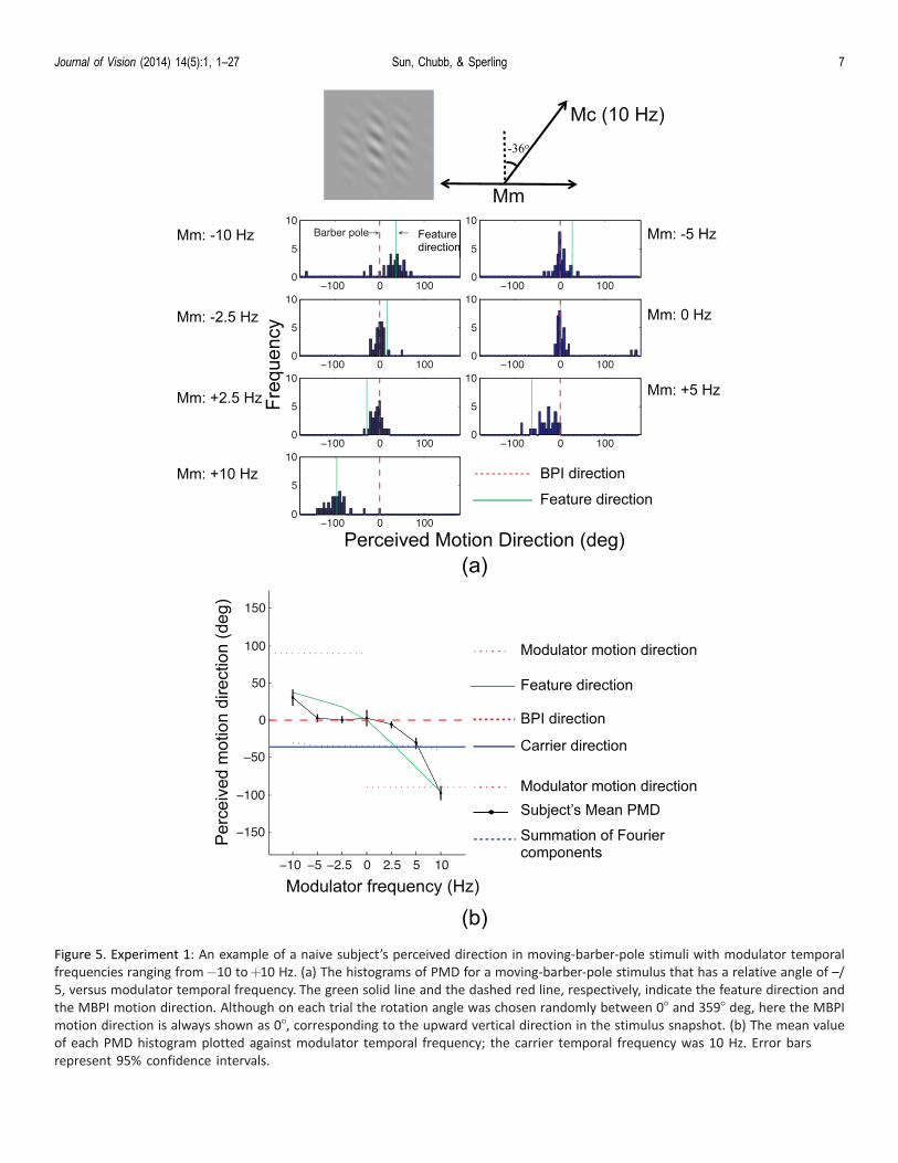
Figure 5. Experiment 1: An example of a naive subject’s perceived direction in moving-barber-pole stimuli with modulator temporal

frequencies ranging from�10 toþ10 Hz. (a) The histograms of PMD for a moving-barber-pole stimulus that has a relative angle of –/

5, versus modulator temporal frequency. The green solid line and the dashed red line, respectively, indicate the feature direction and

the MBPI motion direction. Although on each trial the rotation angle was chosen randomly between 08 and 3598 deg, here the MBPI

motion direction is always shown as 08, corresponding to the upward vertical direction in the stimulus snapshot. (b) The mean value

of each PMD histogram plotted against modulator temporal frequency; the carrier temporal frequency was 10 Hz. Error bars

represent 95% confidence intervals.


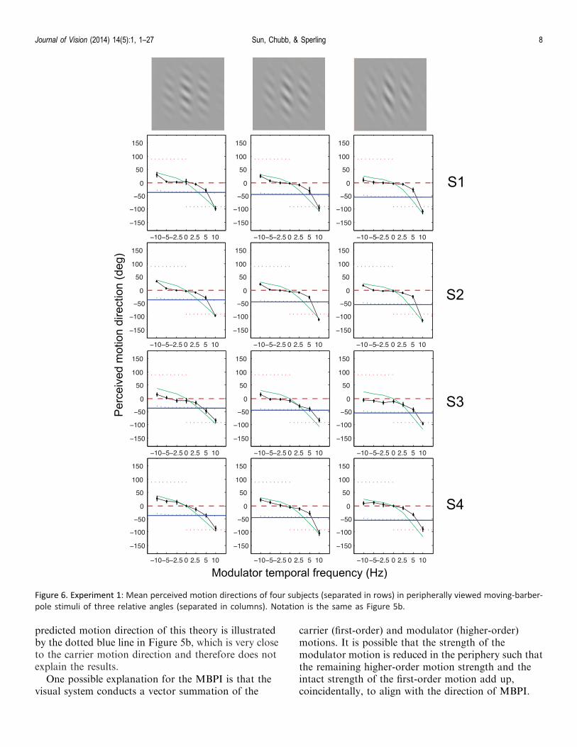
predicted motion direction of this theory is illustratedby the dotted blue line in Figure 5b, which is very closeto the carrier motion direction and therefore does notexplain the results.

One possible explanation for the MBPI is that thevisual system conducts a vector summation of the

carrier (first-order) and modulator (higher-order)motions. It is possible that the strength of themodulator motion is reduced in the periphery such thatthe remaining higher-order motion strength and theintact strength of the first-order motion add up,coincidentally, to align with the direction of MBPI.

Figure 6. Experiment 1: Mean perceived motion directions of four subjects (separated in rows) in peripherally viewed moving-barber-

pole stimuli of three relative angles (separated in columns). Notation is the same as Figure 5b.


Such a summation of first- and higher-order motionvectors has been proposed in other contexts (Tse &Hsieh, 2006; Wilson et al., 1992).

However, even the data in Experiment 1 aloneindicate that the combination of first- and higher-ordermotion is unlikely to explain MBPI. This is because theMBPI prevailed when the modulator was static. PMDwould have been close to pure first-order carrier motion(not MBPI) had it resulted from the combination offirst- and higher-order motions vectors. Also, when thecarrier and modulator moved in the same direction(i.e., when the modulator temporal frequencies werepositive in Figure 5b), PMDs did not fall between thecarrier and modulator motion direction as the combi-nation rule would have predicted. Instead, PMDs fellbetween the MBPI and the feature direction. TheMBPI requires another explanation.

Experiment 2: Carrier temporalfrequency

Experiment 1 tested the dependency of the MBPI onthe higher-order modulator temporal frequency, andfound that the MBPI obtained over a middle range ofmodulator frequencies.

Experiment 2 investigated the effect of varying thecarrier temporal frequency.

Stimuli

Stimuli remained the same except that the relativeangle of the carrier stripes was fixed at –p/4 and threemore carrier temporal frequencies (5, 2.5, 0 Hz) wereincluded. That is, the previous condition of 10 Hzcarrier temporal frequency was interleaved with threemore conditions of the carrier temporal frequency. Ofcourse, when the carrier temporal frequency was 0 Hz,the modulator was never 0 Hz.


Figure 7 shows mean PMDs as functions ofmodulator temporal frequencies at four carriertemporal frequencies. At the carrier temporal fre-quency of 10 Hz, PMDs are essentially identical tothose in Experiment 1. As carrier temporal frequencydecreases, so does the influence of the MBPI directionon the PMD—an indication that MBPI depends onthe carrier temporal frequency. When carrier tempo-ral frequency decreases to zero, PMD is entirely inthe feature direction. In fact, PMDs always lie

between the feature direction and the MBPI motiondirection.

As in Experiment 1, increasing modulator temporalfrequency tends to align PMDs with the featuredirection. Inspection of Figure 7 shows that, althoughcarrier motion and modulator motion both influencePMD, it cannot by simple addition of velocityvectors.

Experiment 3: Phase of adjacentbarber poles

Experiment 2 showed that the MBPI was affected bychanges in the carrier temporal frequency. The carriermotion in the three visible barber poles within acircular Gaussian window in the stimuli of Experiments1 and 2 was derived from the same fundamental sine-wave component (Figure 3d). This configuration maygenerate an implicit computation (or even a percept) ofa single, extended sine wave (rather than of several sinewaves restricted within each pole) moving behindvertical occluders (the zero-contrast regions), especiallyin the periphery. Experiment 3 investigated whetherhaving a single carrier sine-wave component fill allthree barber poles is critical for the MBPI.

Stimuli

The single sine-wave component was effectivelyremoved by reversing the carrier contrast in half of allthe barber poles (see the example in Figure 8). To dothis, the sign of the raised cosine modulator was flippedin every other spatial cycle. Within each pole, however,the carrier motion was perfectly retained despite thismanipulation.


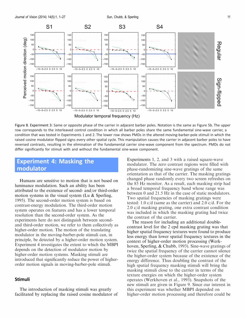
PMDs for the control condition and the contrast-reversed condition are shown in Figure 8. The MBPI isdominant in the control condition (left column) and ishardly affected even when the percept of a single carriermotion is not available (right column). This suggeststhat the computation of the MBPI does not need thecomputation of the single, extended carrier motion. Infact the whole pattern of the PMD curve seemsunaffected. If the computation giving rise to the PMDcurve does involve the computation of the carriermotion, then the carrier motion is probably computedlocally within each pole, rather than over the entirevisible area.


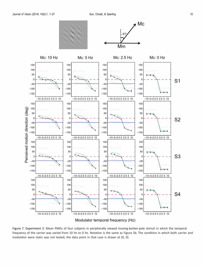
Figure 7. Experiment 2: Mean PMDs of four subjects in peripherally viewed moving-barber-pole stimuli in which the temporal

frequency of the carrier was varied from 10 Hz to 0 Hz. Notation is the same as Figure 5b. The condition in which both carrier and

modulator were static was not tested; the data point in that case is drawn at (0, 0).


Experiment 4: Masking themodulator

Humans are sensitive to motion that is not based onluminance modulation. Such an ability has beenattributed to the existence of second- and/or third-ordermotion systems in the visual system (Lu & Sperling,1995). The second-order motion system is based oncontrast-energy modulation. The third-order motionsystem operates on features and has a lower temporalresolution than the second-order system. As theexperiments here do not distinguish between second-and third-order motion, we refer to them collectively ashigher-order motion. The motion of the translatingmodulator in the moving-barber-pole stimuli can, inprinciple, be detected by a higher-order motion system.Experiment 4 investigates the extent to which the MBPIdepends on the detection of modulator motion byhigher-order motion systems. Masking stimuli areintroduced that significantly reduce the power of higher-order motion signals in moving-barber-pole stimuli.

Stimuli

The introduction of masking stimuli was greatlyfacilitated by replacing the raised cosine modulator of

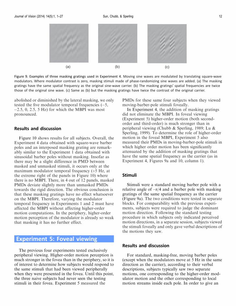
Experiments 1, 2, and 3 with a raised square-wavemodulator. The zero contrast regions were filled withphase-randomizing sine-wave gratings of the sameorientation as that of the carrier. The masking gratingschanged phase randomly every two screen refreshes onthe 85 Hz monitor. As a result, each masking strip hada broad temporal frequency band whose range wasbetween 0 and 21.5 Hz in the case of static modulators.Two spatial frequencies of masking gratings weretested: 1.0 c/d (same as the carrier) and 2.0 c/d. For the2.0 c/d masking grating, one extra contrast conditionwas included in which the masking grating had twicethe contrast of the carrier.

The reason for including an additional double-contrast level for the 2 cpd masking grating was thathigher spatial frequency textures were found to produceless energy than lower spatial frequency textures in thecontext of higher-order motion processing (Werk-hoven, Sperling, & Chubb, 1993). Sine-wave gratings oftwice the spatial frequency of the carrier cannot silencethe higher-order system because of the existence of theenergy difference. Thus doubling the contrast of thehigh spatial frequency masking stimuli will bring themasking stimuli close to the carrier in terms of thetexture energies on which the higher-order systemoperates (Werkhoven et al., 1993). Snapshots of thenew stimuli are given in Figure 9. Since our interest inthis experiment was whether MBPI depended onhigher-order motion processing and therefore could be

Figure 8. Experiment 3: Same or opposite phase of the carrier in adjacent barber poles. Notation is the same as Figure 5b. The upper

row corresponds to the interleaved control condition in which all barber poles share the same fundamental sine-wave carrier, a

condition that was tested in Experiments 1 and 2. The lower row shows PMDs in the altered moving-barber-pole stimuli in which the

raised cosine modulator flipped signs every other spatial cycle. This manipulation causes the carrier in adjacent barber poles to have

reversed contrasts, resulting in the elimination of the fundamental carrier sine-wave component from the spectrum. PMDs do not

differ significantly for stimuli with and without the fundamental sine-wave component.


abolished or diminished by the lateral masking, we onlytested the five modulator temporal frequencies (�5,�2.5, 0, 2.5, 5 Hz) for which the MBPI was mostpronounced.


Figure 10 shows results for all subjects. Overall, theExperiment 4 data obtained with square-wave barberpoles and an interposed masking grating are remark-ably similar to the Experiment 1 data obtained withsinusoidal barber poles without masking. Insofar asthere may be a slight difference in PMD betweenmasked and unmasked stimuli, it occurs only at themaximum modulator temporal frequency (þ5 Hz, atthe extreme right of the panels in Figure 10) wherethere is no MBPI. There, in 4 out of 12 panels, maskedPMDs deviate slightly more than unmasked PMDstowards the rigid direction. The obvious conclusion isthat these masking gratings have no effect whatsoeveron the MBPI. Therefore, varying the modulatortemporal frequency in Experiments 1 and 2 must haveaffected the MBPI without affecting higher-ordermotion computations. In the periphery, higher-ordermotion perception of the modulator is already so weakthat masking it has no further effect.

Experiment 5: Foveal viewing

The previous four experiments tested exclusivelyperipheral viewing. Higher-order motion perception ismuch stronger in the fovea than in the periphery, so it isof interest to determine how subjects would respond tothe same stimuli that had been viewed peripherallywhen they were presented in the fovea. Until this point,the three naive subjects had never seen the testingstimuli in their fovea. Experiment 5 measured the

PMDs for these same four subjects when they viewedmoving-barber-pole stimuli foveally.

In Experiment 4, the addition of masking gratingsdid not eliminate the MBPI. In foveal viewing(Experiment 5) higher-order motion (both second-order and third-order) is much stronger than inperipheral viewing (Chubb & Sperling, 1989; Lu &Sperling, 1999). To determine the role of higher-ordermotion in the foveal MBPI, Experiment 5 alsomeasured their PMDs in moving-barber-pole stimuli inwhich higher order motion has been significantlyattenuated by the addition of masking gratings thathave the same spatial frequency as the carrier (as inExperiment 4, Figures 9a and 10, column 1).

Stimuli

Stimuli were a standard moving barber pole with arelative angle of –p/4 and a barber pole with maskinggratings of the same spatial frequency as the carrier(Figure 9a). The two conditions were tested in separateblocks. For comparability with the previous experi-ments, subjects were required to judge the dominantmotion direction. Following the standard testingprocedure in which subjects only indicated perceivedmotion directions, in a separate session, subjects viewedthe stimuli foveally and only gave verbal descriptions ofthe motions they saw.


For standard, masking-free, moving barber poles(except when the modulators move at 5 Hz in the samedirection as the carrier), according to their verbaldescriptions, subjects typically saw two separatemotions, one corresponding to the higher-order mod-ulator motion and the other corresponding to localmotion streams inside each pole. In order to give an

Figure 9. Examples of three masking gratings used in Experiment 4. Moving sine waves are modulated by translating square-wave

modulators. Where modulator contrast is zero, masking stimuli made of phase-randomizing sine waves are added. (a) The masking

gratings have the same spatial frequency as the original sine-wave carrier. (b) The masking gratings’ spatial frequencies are twice

those of the original sine wave. (c) Same as (b) but the masking gratings have twice the contrast of the original carrier.


Figure 10. Experiment 4: Mean PMDs of four subjects in peripherally viewed moving-barber-pole stimuli with masking gratings that

reduce the influence of higher-order motion-perception mechanisms. Solid black lines connect the data points. The solid red line is

comparison data from Experiment 1 (Figure 6, middle column) obtained without masking gratings. Other notation is the same as

Figure 5b. Columns are arranged in the same order as in Figure 9.


estimate of only one dominant motion, they variouslyresponded to either one of the motions or theyresponded with an arbitrary compromise between thosemotions. When the modulator moved at 5 Hz in thesame direction as the carrier, they saw a single coherentmotion (the feature, i.e. rigid motion).

PMDs for standard moving barber poles are given inthe first row of Figure 11. No obvious MBPI is presentcompared to the same stimuli viewed peripherally(Figure 6). Interestingly, in some conditions, the meanPMDs are close to the higher-order modulator motiondirection, which never occurred in the peripheralviewing condition. Large error bars indicate that PMDsobtained in the fovea are diverse. When plotted ascircular histograms (Figure 12), PMDs are indeed verydiverse and sometimes show multi-modality patterns.In other words, when the higher-order modulatormotion is available to the motion system, it does nothelp form the MBPI motion but instead masks it. Onthe other hand, attenuating the higher-order modulatormotion with the masking gratings in foveal viewing(Figure 11, bottom row) or by peripheral viewing(Figure 6) greatly facilitates the MBPI.

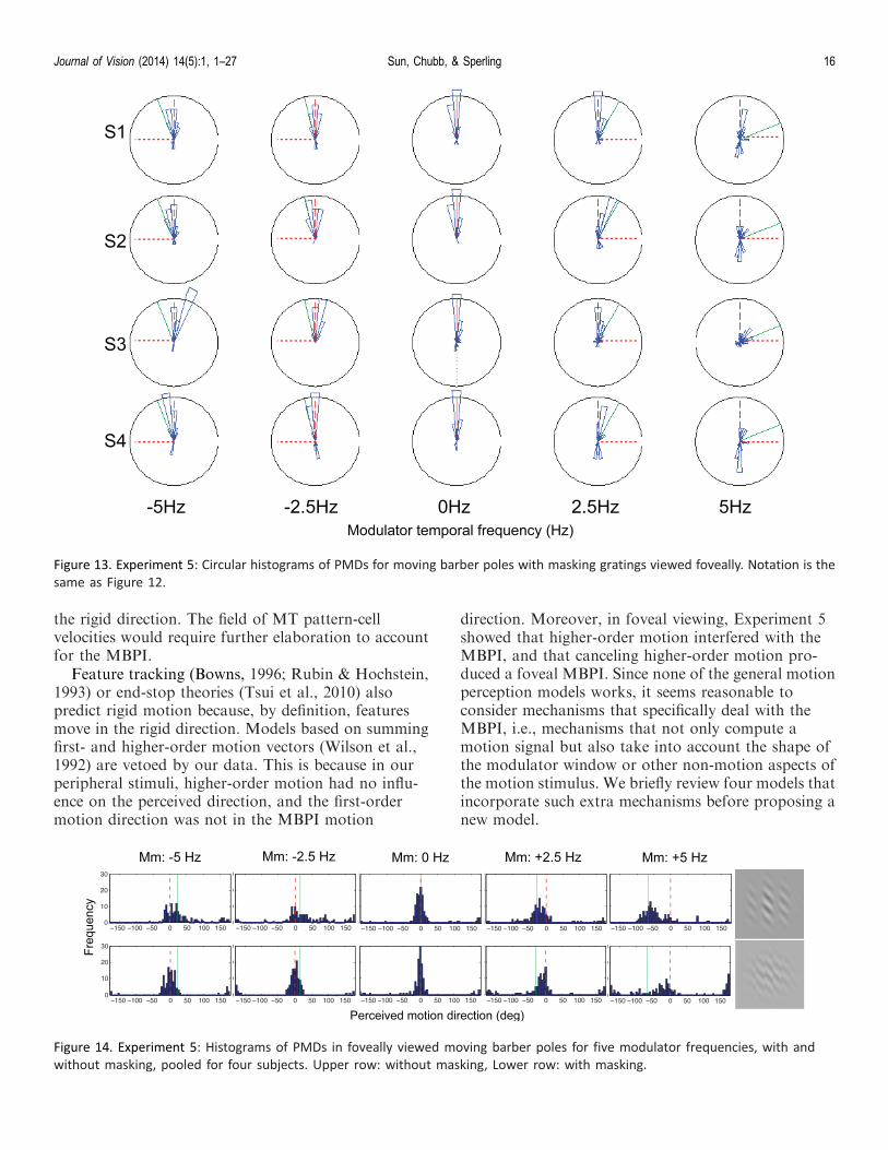
In contrast to the diverse histograms in foveallyviewed standard moving-barber-pole stimuli, with theaddition of masking gratings, the circular histograms ofPMDs become more compact and centered on theMBPI direction, as shown in Figure 13. This isespecially true when the modulator moves in theopposite direction of the carrier. Also notable in Figure13 is that sometimes PMD is in the reversed direction ofMBPI. In some cases this might be due to a confusion

of random motion components of the interleavedmasking gratings with the motion of the moving-barber-pole grating. However, the frequency of re-versed versus normal MBPI directions in several of thepanels of Figure 13 suggests the possibility of reversedMBPI.

Note that the mean PMDs for S4 in the lower rightpanel of Figure 11 are not in the same range as thosefor the other three subjects. But S4’s circular histo-grams under the two conditions (the rightmost twopanels in the bottom row in Figure 13) reveal that thissubject frequently perceived a reversed MBPI. Theaverage of MBPI and reverse MBPI gives an unusualangle. Apart from this one case, the other mean PMDsfor the masked moving barber poles clearly demon-strate the change of PMDs from an irregular, randompattern (first row) to a MBPI dominated pattern(second row). In other words, the addition of thebetween pole masking gratings restored MBPI in thefoveal view.

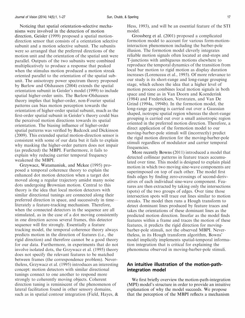
Figure 14 shows histograms of PMDs pooled for allsubjects. For regular moving-barber-pole stimuli (toprow), the component of MBPI is either swampedamidst the broad range of the responses (e.g., formodulator frequency�5 and�2.5 Hz) or is very weakcompared to the component of the rigid direction (e.g.,for modulator frequencyþ2.5 and þ5 Hz). Of coursefor 0 Hz, a stationary modulator, i.e., a classical barberpole, a normal BPI is observed. When the modulator ismasked (bottom row), PMDs clearly peak around theMBPI direction for almost all modulator temporalfrequencies. The exception is þ5 Hz modulator

Figure 11. Experiment 5: Mean PMDs for foveally viewed moving barber poles with masking gratings (bottom row) and without (top

row).


frequency, in which case there is a secondary peakaround the reversed MBPI direction.

Even in the case of a stationary modulator, themasking grating compresses the histogram of PMDs,i.e., it improves the classical BPI. This is contrary to theobservations of Lalanne (2006) who found that lateralmasking and adaptation impaired the BPI. This may bedue to the use of a much lower temporal frequency ofthe carrier (2.5 and 3.3 Hz) than the 10 Hz in thepresent study. Lower temporal frequencies makepossible the involvement of higher-order motionprocesses in the perception of carrier motion.

Review

In the moving-barber-pole stimulus, the directions ofrigid motion (same as feature motion), first-ordermotion, higher-order motion, MBPI motion are alldifferent. However, the fact that MBPI is consistentlyperceived over a wide range of parameters is notpredicted by any current model or theory. We consider

here what current motion perception models do predictas the direction of perceived motion in moving-barber-pole stimuli.

We begin with the most general motion-perceptionmodels.

For moving-barber-pole stimuli, models based onthe principle of computing the rigid direction (Heeger,1987; Schrater, Knill, & Simoncelli, 2000) predict therigid-motion direction, not the MBPI motion direction.We consider the predicted response to moving-barber-pole stimuli of two models of MT pattern cells(Perrone, 2004; Simoncelli & Heeger, 1998). A distinc-tive feature of MT pattern cells is that they are sensitiveto the direction of the corresponding rigid translationof a pattern, rather than directions of Fouriercomponent motions. These MT pattern cell models aresensitive to the rigid direction not the MBPI directionof the moving-barber-pole stimulus. Perrone (2012)used one of the MT pattern cell models (Perrone, 2004)to generate a field of local velocities (speeds anddirections), on which further processing could beoperated. For the moving-barber-pole stimulus, wewere able to show that these velocity vectors all point in

Figure 12. Experiment 5: Circular histograms of PMDs for moving barber poles without masking gratings viewed foveally. Rows

represent subjects, columns represent modulator temporal frequencies. Each bin is 108 wide. The boundary of the circle corresponds

to 10/30 trials. The dashed red lines represent the MBPI direction. The horizontal dashed red lines represent the modulator direction

except at 0 Hz when there is no modulator motion. The solid green lines represent the rigid (feature) direction.


the rigid direction. The field of MT pattern-cellvelocities would require further elaboration to accountfor the MBPI.

Feature tracking (Bowns, 1996; Rubin & Hochstein,1993) or end-stop theories (Tsui et al., 2010) alsopredict rigid motion because, by definition, featuresmove in the rigid direction. Models based on summingfirst- and higher-order motion vectors (Wilson et al.,1992) are vetoed by our data. This is because in ourperipheral stimuli, higher-order motion had no influ-ence on the perceived direction, and the first-ordermotion direction was not in the MBPI motion

direction. Moreover, in foveal viewing, Experiment 5showed that higher-order motion interfered with theMBPI, and that canceling higher-order motion pro-duced a foveal MBPI. Since none of the general motionperception models works, it seems reasonable toconsider mechanisms that specifically deal with theMBPI, i.e., mechanisms that not only compute amotion signal but also take into account the shape ofthe modulator window or other non-motion aspects ofthe motion stimulus. We briefly review four models thatincorporate such extra mechanisms before proposing anew model.

Figure 13. Experiment 5: Circular histograms of PMDs for moving barber poles with masking gratings viewed foveally. Notation is the

same as Figure 12.

Figure 14. Experiment 5: Histograms of PMDs in foveally viewed moving barber poles for five modulator frequencies, with and

without masking, pooled for four subjects. Upper row: without masking, Lower row: with masking.


Noticing that spatial orientation-selective mecha-nisms were involved in the detection of motiondirection, Geisler (1999) proposed a spatial motion-direction sensor that consists of a orientation selectivesubunit and a motion selective subunit. The subunitswere so arranged that the preferred directions of themotion unit and the orientation of the spatial unit wereparallel. Outputs of the two subunits were combinedmultiplicatively to produce a response that peakedwhen the stimulus motion produced a motion streakoriented parallel to the orientation of the spatial sub-unit. The anisotropy power spectrum theory proposedby Barlow and Olshausen (2004) extends the spatialorientation subunit in Geisler’s model (1999) to includespatial higher-order units. The Barlow-Olshausentheory implies that higher-order, non-Fourier spatialpatterns can bias motion perception towards theorientation of higher-order spatial subunit, much as thefirst-order spatial subunit in Geisler’s theory could biasthe perceived motion directions towards its spatialorientation. The biasing influence of higher-orderspatial patterns was verified by Badcock and Dickinson(2009). This extended spatial motion-direction sensor isconsistent with some of our data but it fails to explainwhy masking the higher-order pattern does not impair(as predicted) the MBPI. Furthermore, it fails toexplain why reducing carrier temporal frequencyweakened the MBPI.

Grzywacz, Watamaniuk, and Mckee (1995) pro-posed a temporal coherence theory to explain theenhanced dot motion detection when a target dotmoved along a regular trajectory amidst many noisedots undergoing Brownian motion. Central to thistheory is the idea that local motion detectors withsimilar directional tunings are connected along theirpreferred direction in space, and successively in time—literately a feature-tracking mechanism. Therefore,when the connected detectors in the sequence are allstimulated, as in the case of a dot moving consistentlyin one direction across several frames, this detectorsequence will fire strongly. Essentially a featuretracking model, the temporal coherence theory alwayspredicts motion in the direction of features (i.e., therigid direction) and therefore cannot be a good theoryfor our data. Furthermore, in experiments that do notinvolve isolated dots, the Grzywacz et al. (1995) theorydoes not specify the relevant features to be matchedbetween frames (the correspondence problem). Never-theless, Grzywacz et al. (1995) introduces an interestingconcept: motion detectors with similar directionaltunings connect to one another to respond morestrongly to coherently moving objects. Coherentdirection tuning is reminiscent of the phenomenon oflateral facilitation found in other sensory domains,such as in spatial contour integration (Field, Hayes, &

Hess, 1993), and will be an essential feature of the STImodel.

Grossberg et al. (2001) proposed a complicatedformotion model to account for various form-motion-interaction phenomenon including the barber-poleillusion. The formotion model cleverly integratesreliable motion signals often located at end-stops andT-junctions with ambiguous motions elsewhere toreproduce the temporal dynamics of the transition fromlocal bar motion to rigid motion as display durationincreases (Lorenceau et al., 1993). Of more relevance toour study is its short-range and long-range groupingstage, which echoes the idea that a higher level ofmotion process combines local motion signals in bothspace and time as in Van Doorn and Koenderink(1984) and Fredericksen, Verstraten, and Van DeGrind (1994a, 1994b). In the formotion model, thelong-range grouping is carried out over a Gaussianshaped, isotropic spatial region whereas the short-rangegrouping is carried out over a small anisotropic regionoriented in the preferred motion direction. Therefore, adirect application of the formotion model to ourmoving-barber-pole stimuli will (incorrectly) predictthe rigid motion direction for the moving-barber-polestimuli regardless of modulator and carrier temporalfrequencies.

More recently Bowns (2011) introduced a model thatdetected collinear patterns in feature traces accumu-lated over time. This model is designed to explain plaidmotion in which two moving sine-wave components aresuperimposed on top of each other. The model firstfinds edges by finding zero-crossings of second-deriv-atives of each individual sine-wave component. Fea-tures are then extracted by taking only the intersections(spots) of the two groups of edges. Over time thoseintersection spots will trace out lines similar to motionstreaks. The model then runs a Hough transform todetect dominant lines produced by feature traces andtakes the orientations of these dominant lines as thepredicted motion direction. Insofar as the model findsfeatures within a frame and traces the motion of thesefeatures, it predicts the rigid direction for moving-barber-pole stimuli, not the observed MBPI. Never-theless, in its Hough transform algorithm, Bowns’model implicitly implements spatial-temporal informa-tion integration that is critical for explaining thephenomena observed in moving-barber-pole stimuli.

An intuitive illustration of the motion-path-integration model

We first briefly overview the motion-path-integration(MPI) model’s structure in order to provide an intuitiveexplanation of why the model succeeds. We proposethat the perception of the MBPI reflects a mechanism


that operates over a relatively large spatial area andprolonged time period. In Bowns’ (2011) model, amoving feature leaves a trace. In the MPI model, thechanging location of local motion energy leaves a trace.Like feature traces, local motion energy traces for agiven image sequence are functions of both space andtime. Consider for example a moving barber-polestimulus, our standard stimulus, in which the modula-tor moves at a relatively slow temporal frequencyoppositely to the carrier (Figure 15a). To simplifyFigure 15, the sine-wave carrier and modulator areboth represented as square-waves. The feature extrac-tion process (described in detail below) produces thebright regions of the carrier square-wave (the brightregions in Figure 15). These features move in aconsistent direction (i.e., the feature direction) as aresult of the carrier’s and modulator’s cooperativemovement. Figure 15b shows the locations of those

features across four frames. Alternatively, Figure 15can be thought of as the 2-D projection (i.e., the 2-Dretinal image) of the three-dimensional (3-D) spatial-temporal feature function over four frames. In Figure15d through f, the local motion energy traces are shownbased on this 2-D projection of the 3-D featurefunctions.

In a 2-D motion signal, local motion energy at apoint exists in many directions. In Figure 15 we showmotion energies, represented as vectors, along threedirections: the barber-pole direction (Figure 15d), thefeature direction (Figure 15e) and the carrier motiondirection (Figure 15f). In each of Figure 15d, e, and f,dots (instead of vectors) represent points with zerolocal motion energy in the corresponding direction.Regions outside of the barber-pole windows (i.e., zerocontrast regions) contain mostly zero motion energiesin all directions. The solid arrows indicate the motion

Figure 15. Examples of local motion energy traces for a moving-barber-pole stimulus in which the modulator moves to the left at 2.5

Hz and the carrier moves up to the right at 10 Hz. The carrier and the modulator are represented as square-waves with the dark

regions set equal to the background. (a) Snapshot of a single frame. (b) Four consecutive frames shown together. For clarity, features

in frames 2, 3, and 4 are shown in lower contrast. Bars with the same number belong to the same frame in the image sequence. (c)

For clarity, the carrier is represented as square-waves. (d–f) Illustrations of local motion energies along the barber-pole direction, the

feature direction, and the carrier motion direction, respectively. In each figure, spots represent points where local motion energies

are zero. Solid arrows indicate motion energies between frames 1 and 2; dashed arrows indicate motion energies between frames 3

and 4.


energies computed between frames 1 and 2; the dashedarrows indicate the motion energies computed betweenframe 3 and 4. Motion energies between frame 2 and 3are similar but are not drawn to reduce clutter. Motionenergies for different frame pairs are labelled distinc-tively to reflect the fact that local motion energies varywith time. Although they are drawn in one figure panel,they actually appear in different frames in time. In thisexample, along the barber-pole direction (Figure 15e),both solid and dashed arrows connect to one another toform a consistent vertical pattern. Along the other twodirections (Figure 15e, f), the vector connections areinterrupted by zero motion energy regions. Therefore amechanism that integrates local motion energies overan elongated region and over limited time period (i.e.,one cycle of a 10 Hz stimulus) can potentially explainthe peripheral MBPI in this stimulus. It is worth notingthat the advantage of a vertical connection over otherconnections disappears when motion energies aretraced for longer time period. The time period includedin the integration is critical. If the time period includedin the feature trace were to increase significantly, thevertical direction of Figure 15d would lose itsadvantage to the feature tracking direction of Figure15e. The temporal coherence theory (Grzywacz et al.,1995) implicitly integrates over a large number offrames and therefore predicts that the feature (not theMBPI) direction would be perceived in this stimulus.

Model implementation

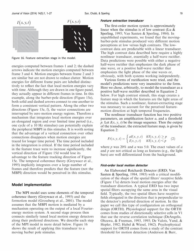
The MPI model uses some elements of the temporalcoherence theory (Grzywacz et al., 1995) and theformotion model (Grossberg et al., 2001). The modelassumes that the MBPI motion is mediated by amechanism operating on the output of a local Fourier-energy motion system. A second stage process thenconnects similarly tuned local motion energy detectorsalong their preferred directions. We describe each stepof the MPI model in more detail below. Figure 16shows the result of applying this transducer to amoving barber pole stimulus.

Feature extraction transducer

The first-order motion system is approximatelylinear when the stimulus is of low contrast (Lu &Sperling, 1995; Van Santen & Sperling, 1984). Inunpublished experiments, we found that the moving-barber-pole stimulus produced very different motionperceptions at low versus high contrasts. The low-contrast data are predictable with a linear transducer.The high contrast data described here require a highlynonlinear transducer, essentially a half-wave rectifier.Data predictions were possible with either a negativehalf-wave rectifier that emphasizes the dark phase ofsine wave, or a positive half-wave rectifier thatemphasizes the light phase of the sine waves or,obviously, with both systems working independently.

Various forms of rectification were tried, and themodel’s predictions were very insensitive to the form.Here we chose, arbitrarily, to model the transducer as apositive half-wave rectifier described in Equation 2below. For high contrast stimuli, this stage creates afeature map in which the features are the light areas ofthe stimulus. Such a nonlinear, feature-extracting stagewas necessary to account for the perceived feature-motion direction at high temporal frequencies.

The nonlinear transducer function has two positiveparameters, an amplification factor a, and a thresholdp. Let I(x, y, t) be the image sequence. Then the outputof the transducer, the extracted feature map, is given byEquation 2:

Ftðx; y; tÞ ¼ aIðx; y; tÞ ifIðx; y; tÞ � pIðx; y; tÞ ifIðx; y; tÞ, p

�ð2Þ

where p was 20% and a was 5.0. The exact values of aand p are not critical as long as features (e.g., the lightbars) are well differentiated from the background.

First-order local motion detector

An Elaborated Reichardt Detector (ERD; VanSanten & Sperling, 1984, 1985) with a critical modifi-cation of the shape of the spatial filters’ receptive fields(Figure 17a) detects local motion energies after thetransducer distortion. A typical ERD has two inputspatial filters occupying the same area in the visualfield. Typically, the two spatial filters have receptivefields elongated in the direction that is perpendicular tothe detector’s preferred direction of motion. In thispaper we call this type of configuration an orthogonaldesign (ORTH). Physiological support for the ORTHcomes from studies of directionally selective cells in V1that use the reverse correlation technique (DeAngelis,Ohzawa, & Freeman, 1993, 1995; De Valois, Yund, &Hepler, 1982; Hubel & Wiesel, 1962). Psychophysicalsupport for ORTH comes from a study of the contrastthreshold for motion detection (Anderson & Burr,

F x, y, t( )I x, y, t( )

Figure 16. Feature extraction stage in the model.


1991). However, evidence also exists for a differentreceptive field shape in which the spatial receptive fieldis elongated in the same direction as the motiondetector’s preferred direction (Fredericksen et al.,1994a, 1994b; Geisler et al., 2001; Jancke, 2000; VanDoorn & Koenderink, 1984). We call this type ofconfiguration an extended design (EXT). A recentstudy shows that EXT can help in detecting prolongedmotion such as motion streaks (as opposed to short-lived, brief motion; Pavan et al., 2011). The evidencesuggests that two quite different receptive field config-

urations both exist but may be differentially effectivedepending on stimulus contrast and other factors.1 Toaccount for our data, it was necessary to use a EXTdesign for our ERD’s spatial receptive field; based onFredericksen et al. (1994b) and Van Doorn andKoenderink (1984), we chose an aspect ratio of 10 : 1.Finally, the bandwidth of the spatial filter was fixed at 1octave. Defining the bandwidth in terms of octavesmeans that the configuration of the spatial filter scaleswith the filter’s optimal spatial frequency.

In addition to the spatial filters, the ERD has twotemporal filters. The first temporal filter (TF in Figure17b) reflects the low- and band-pass characteristic ofhuman observers’ temporal sensitivity (Robson, 1966;Watson & Ahumada, 1985). The impulse function isdepicted by the red curve in Figure 17b. The secondtemporal filter (TD in Figure 17b) is a first-order, low-pass filter with an impulse response defined by e�t/s for t� 0, and 0 for t , 0. TD delays its input and thisdelayed input is compared with the undelayed input inthe multiplier unit, ·. The impulse function of thetemporal filter combining the first and second temporalfilters is depicted by the green curve in Figure 17b. Thisconfiguration and the characteristics of the temporalfilters are largely consistent with conventional modelsof motion energy detectors (Adelson & Bergen, 1985;Van Santen & Sperling, 1985; Watson & Ahumada,1985).

The responses of the ERDs are normalized by thesize of their receptive fields (not shown in Figure 17) toensure that all ERDs, independent of their spatialfrequency tuning, respond with equal intensity whenpresented with their optimal stimulus. For a givendirection, the MPI model considers only the ERDoptimally tuned to the spatial frequency along thatgiven direction. To find the optimal spatial frequency inthe moving-barber-pole stimuli for every direction, wefirst calculated the optimal spatial frequencies analyt-ically. Then a computer simulation was conducted toensure that ERDs with those optimal spatial frequen-cies indeed produced the strongest response. Tocharacterize the first-stage operation, we define ERDhi

as the ERD that is tuned in the direction hi and thatcontains optimally tuned spatial filters in the directionhi. The output of the Local Motion Energy Detectorstage is a field of local motion energies Ei(x, y, t) in thedirection hi:

Eiðx; y; tÞ ¼ ERDhiðFtðx; y; tÞÞ ð3ÞThe MPI model assumes a second stage mechanism

that integrates the output from the Local MotionEnergy Detector over a relatively large area at a limitedtime interval. Each component unit of the second-stagemechanism has its own directional tuning property(Figure 18a). It aggregates half-rectified responses froman array of local ERDs that are tuned to the same

Figure 17. Diagrams of the local motion detector components of

the MPI model. (a) A typical ERD. Spatial filters are elongated

perpendicularly to the detector’s preferred motion direction

(Van Santen & Sperling, 1984, 1985). (b) The ERD used in the

MPI model has spatial filters extended in the detector’s

preferred direction (EXT). In (a) and (b), detector’s preferred

motion direction is horizontal, with positive outputs indicating

rightward motion. (c) The impulse response of the temporal

filter TF and the impulse response after passing through TD, TF

· TD. (d) Illustration of the range of directions to which ERDs

are tuned. The striped ovals indicate ERDs as illustrated in (b)

tuned to the directions of the arrows. The full range of motion

directions is assumed to be represented in every local area in

the region of interest.


direction as the second stage mechanism. This aggre-

gation is carried out over a limited time period r along

a spatial path that is in the common preferred direction

hi of the MPI model’s first- and second-stage mecha-

nisms. To improve the directional selectivity of the

second-stage mechanism, a lateral inhibition region

that flanks the spatial integration path is included.

Together, the integration and inhibition area form a

higher-order receptive field for the second stage

mechanism. We implemented the integration process by

applying a 3-D Gabor filter to the local motion energies

(Equation 3) computed by the previous stage. To

describe the second-state integration we need to define

the following:

First, let Gi(x, y, t) be a 3-D Gabor filter thataggregates local motion energies at a point x, y andtime t a long the direction hi

Giðx; y; tÞ ¼ expð� ðx cos hi þ y sin hiÞ2

2r2x

� ðy cos hi � x sin hiÞ2

2ðrx

a Þ2

Þcosð2p/ðx cos hi

þ y sin hiÞÞexpð� t2

2r2t

Þ

ð4ÞThe 3-D Gabor filter Gi(x, y, t) can be thought of as

a stack of spatial 2-D Gabor filters whose amplitudesare modulated by a temporal Gaussian functionexpð� t2

2r2tÞ.

Then let Li(x, y, t) be a weighed sum of the localmotion energies Ei(x, y, t) along the direction hi

Liðx; y; tÞ ¼RRR

Giðx� c; y� g; t� sÞEiðc; g; sÞdcdgds

ð5ÞThe response, RESi, of a second-stage mechanism

with a preferred direction of hi, is given by the variance,i.e., the power, of Li(x, y, t) that can be understood as ameasure of response amplitude of the higher-orderreceptive field. RESi gives the total power in thedirection hi over the whole stimulus for its entireduration.

RESi ¼ VarðLiðx; y; tÞÞ ð6ÞFinally the predicted motion direction PMD is given

by the mean of the responses RESi over all simulateddirections.

PMD ¼

Xni¼1

hiRESi

Xni¼1

RESi

ð7Þ

The full MPI model is outlined in Figure 19.Explanation of model parameters: The model has threefree parameters, all concerning the characteristic of thesecond-stage mechanism. The first free parameter a isthe aspect ratio of the 3-D Gabor filter that is used toimplement the spatial-temporal motion energy inte-gration. a controls the elongation of the higher-orderreceptive field. A more elongated higher-order receptivefield extends the spatial integration area, hencepromoting detection of barber-pole motion. Thesecond free parameter rt controls the temporalintegration window. Increasing rt increases the model’sfeature tracking capability.

The parameter u controls lateral inhibition. Lateralinhibition in motion integration is similar to the optimal

Figure 18. Diagrams for the second-stage mechanism. (a) A

directionally tuned, higher-order mechanism aggregates half-

wave-rectified responses of local motion energy detectors. The

aggregation is carried out along a path that is inline with the

higher-order mechanism’s preferred direction. Two weak

inhibitory regions are added flanking the aggregation region to

improve the mechanism’s directional selectivity. (b) Higher-

order mechanisms tuned to various directions.


integration area for shearing motion (Golomb, Ander-sen, Nakayama, MacLeod, & Wong, 1985). In a typicalshearing motion, the velocity of the moving elementsvaries as a function of positions along the axisperpendicular to the direction of motion. In oneexperiment in Golomb et al.’s (1985) study, the shearingmotion was made of a field of random dots movinghorizontally. The velocity within each row was constantbut varied vertically following a sinusoidal function ofvertical positions. Dots in different rows could move inopposite directions and some rows could be completelystatic. It was reported that the detectability of this kindof shearing motion varied with the spatial frequency ofthe vertical sinusoidal function, peaking at about 0.6–0.7 c/d. Modulations of lower spatial frequencyimpaired the detection of the vertical sinusoid modula-tion, indicating the existence of an optimal integrationarea being flanked by a lateral inhibition region.

Model prediction

To derive predictions of our data, we first consideronly the moving-barber-pole stimuli of 10 Hz carrier

temporal frequency with the seven different modulatorfrequencies. The two stage processes constitute acompound mechanism that is directionally tuned(Figure 18b). We applied the two-stage mechanismstuned to 36 different directions. Because of computa-tional limitations, a coarse grid search (seven days) wasused to find approximately optimal values for u, a, andrt. Interestingly, all parameters have great degrees oftolerance; when u varies between 0.8 c/d and 1.2 c/d, rt

varies between 40 ms and 80 ms and a varies between0.3 and 1.2, the accounted data variance only variesbetween 80% and 92%. The semi-optimal parameterrange is summarized in Table 1.

Figure 20a shows model responses RESi as functionsof the preferred direction hi, produced by a modelimplementation with a set to 0.5, rt set to 60ms and uset to 0.8 c/d. We deliberately choose to use the lowestpossible value for u to be consistent with the optimalintegration area found in Golomb et al. (1985). Figure20b shows the predicted motion direction (solid blackline) for each of the seven modulator temporalfrequencies. With the choice of these three values, themodel accounts for 90% of the variance in the data. The

Figure 19. Functional flowchart for the MPI model. In the initial nonlinear process, all input image intensities that exceed a certain

threshold are amplified. The resultant image sequence is processed by an ensemble of special motion channels tuned to a full range

of directions. Within each directionally tuned special channel, local motion energies are computed by a spatially distributed array of

ERDs whose spatial input units are elongated in the direction of the ERDs’ preferred motion direction. The output of each ERD is half-

wave rectified; thereby the output is positive only in the preferred and not the anti-preferred direction. The rectified output of an

array of similar ERDs is integrated along a spatial path that is parallel with the ERDs’ preferred direction, i.e., the outputs are passed

through a low-pass temporal filter and a 2-D spatial filter whose profile matches the spatial integration path. The motion-power of

each directionally tuned channel is normalized by the total power of all channels. A subsequent process (not shown) computes the

mean direction of the normalized vector of directional motion outputs.


model describes the essential features of these data:perception of the rigid motion direction when themodulator moves rapidly either with or opposed to thecarrier motion, and the barber-pole motion direction inbetween.

To find the optimal parameter set for other carriertemporal frequencies, in principle one should runsimulations with all possible parameters to each humandata set, which is very computationally intensive.However we find that the parameter set obtained forthe 10 Hz carrier temporal frequency conditionautomatically fits other carrier temporal frequencieswell. Figure 21 gives examples of the MPI modelpredictions for stimuli with carrier temporal frequencyof 10, 5, 2.5, and 0 Hz. The model predictionsuccessfully captures the transition of the MBPI motionto the rigid motion as the carrier temporal frequencydecreases. Using the same parameter values as men-tioned above, the total accounted variance for stimuliof four different carrier frequencies is 97%.

Discussion: Isolating a singlemechanism?

The novel moving-barber-pole stimulus allows us todiscriminate between various motion computationsbecause of the different predictions they make for theperceived direction of the stimulus motion. Bothperipheral viewing of the stimulus and high temporalfrequencies reduce the contributions of higher-ordermotion computations (Lu & Sperling, 1995, 1999) andof other possible complex mechanisms. Ideally, thisimpoverished stimulus isolates a single mechanism thatis responsible for the observed MBPI. The MPI modelwas developed to explain the computations of thismechanism. The MPI model successfully accounted forthe data from the full range of peripherally viewedstimuli, and also for foveally viewed stimuli whenhigher-order motion was cancelled. In the special caseof a stationary modulator, in the peripheral viewingconditions explored in this study, the MPI model alsoaccounted for the classic BPI. In central vision (Figure

11) and at low or intermediate temporal frequencies,other mechanisms came into play.

The MPI model proposes a regime in which locallydistributed, low-level motion sensitive neurons areconnected to a higher-level processing stage thataggregates motion energies in a particular directionwithin a defined time period. Somewhat similar neuralconnections to extract object contours from commonmotion signals were proposed by Ledgeway and Hess

Free parameters Values

/ 0.8;1.2 c/d

a 0.3;1.2

rt 40;60 ms

Table 1. Free parameters and their optimal values for themoving-barber-pole stimulus with carrier temporal frequency of10 Hz. Notes: The parameter / controls lateral inhibition. acontrols the elongation of the higher-order receptive field. rt

controls the temporal integration window.

Figure 20. Model predictions for moving-barber-pole stimuli of

seven modulator temporal frequencies. The carrier temporal

frequency is always 10 Hz. (a) A compound, directionally tuned

mechanism’s response as functions of the mechanisms’ tuned

direction. Each panel corresponds to a stimulus of a particular

modulator temporal frequency presented in the same format as

in Figure 5a. The green solid line indicates the rigid direction

and the dashed red line indicates the barber-pole direction. (b)

The predicted motion direction as a function of the modulator

temporal frequency. Each prediction value is obtained by

finding the mean of the response distribution curve in each

panel in (a). Asterisks represent the mean of the four subjects’

responses. Error bars represent 95% confidence intervals.

Predicted motion directions account for 90% of the data

variance.


(2002, 2006) and by Watamaniuk, McKee, andGrzywacz (1995) to extract extended motion paths.

Many higher-order motion computations such as thecomputation of heading direction and of 3-D structurefrom 2-D motion are based on initial low-level motioncomputations that critically involve velocity. The MPImodel specifically uses only directional motion energyand does not explicitly involve velocity.

Summary and conclusions

The moving-barber-pole display

The normal BPI is a phenomenon that reflects theinfluence of form (the window through which a gratingis perceived) on the perception of motion (the directionin which the grating appears to move). To betterunderstand the mechanism underlying the form-motioninteraction, the current study introduced a novelmoving-barber-pole display. The moving-barber-poledisplay has a translating, rather than a static, modu-lator window. Therefore, the rigid direction (i.e., thedirections of 2-D spatial features such as end-stops), isdifferent from the orientation of the modulatorwindow. The moving-barber-pole display effectivelydifferentiates three different motion directions: therigid motion direction (which includes the direction ofend stops and of other features), the motion directionof the main Fourier components, and motion in thedirection of an elongated modulator window.

The MBPI

Displays were viewed peripherally and at hightemporal frequencies in order to minimize the influenceof higher-order motion computations and thereby toisolate a single motion mechanism. In peripheralviewing, three of four subjects reported strong MBPI

(i.e., the perceived motion direction was in line with theorientation of the modulator window), the fourthsubject’s perceived direction was slightly deviated.When masking signals were added in between themodulator windows, the MBPI was retained by theother three. In the fovea, perceived motion was morecomplicated, due at least in part to concurrentperception of the higher-order modulator motion thatwas not visible in the periphery. Adding a maskingpattern to interfere with the higher-order modulatormotion produced a pure MBPI in the fovea. Thatreducing the subjects’ ability to perceive the modula-tor’s orientation strengthens the MBPI means that theMBPI does not utilize the perceived modulatororientation, which in turn means that motion-streakmodels do not apply to the MBPI. Based on theseobservations, we conclude that the BPI generated bythe moving-barber-pole stimuli was neither a result offeature tracking nor a combination of the first-ordercarrier motion with the higher-order modulator mo-tion, nor a combination of perceived orientation of themodulator with the carrier motion.

Two other results: In peripheral viewing, reducingthe carrier temporal frequency shifted the perceivedmotion direction away from the barber-pole directionand ultimately in the direction of the rigid motion. Howthe transition between the rigid motion direction(feature motion direction) and the MBPI depends oncarrier and modulator temporal frequencies is animportant feature of the experimental results thatpotentially can be used to discriminate betweentheories. Changing the phase of motion in adjacentbarber poles had no effect on the MBPI, showing that,at an early stage, the MBPI is computed within abarber pole, not between barber poles.

The MPI model

A three-stage MPI model was proposed. First, localmotion energies are computed by ERDs whose spatialinput units are elongated in the direction of the ERD’spreferred motion direction. Unlike typical motionmodels, the ERD’s motion receptive fields are elon-gated parallel with rather than perpendicular to themotion direction (EXT design). The EXT design iscritical for the predictions. Then, the local motionenergies are integrated along linear spatial paths (in alldirections) and over a time period of 40–60 ms. Theprecise length of the path was not critical in the model.Finally, the predicted motion direction is given by thevector mean of the responses over all directions. TheMPI model embodies entirely feed-forward computa-tions. It accounts for the large variety of observed BPIphenomena entirely within the motion system and does

Figure 21. Model predictions for the moving-barber-pole stimuli

in which the temporal frequency of the carrier varies from 10

Hz (the left-most column) to 0 Hz (the right-most column). The

model prediction accounts for 97% of the total data variance.


not require any information computed in shape or formsystems.

It was not technically feasible to estimate optimalparameters for the MPI model. Even with merely three‘‘good’’ parameters (temporal integration period, pathlength, and path spatial frequency), the model accountswith great accuracy for a variety of very different data,i.e., the change from MBPI to rigid (feature) motiondirection with carrier temporal frequency, the interac-tion of modulator and carrier temporal frequencies,and the dependence on local versus global stimulusfactors.

Keywords: 2D motion, form-motion-interaction, Bar-ber-Pole-Illusion, motion integration, motion model

Acknowledgements

This work was supported by NSF Award BCS-0843897. We thank the two anonymous reviewers fortheir suggestions that helped to greatly improve thequality of the manuscript.

Commercial relationships: none.Corresponding author: Peng Sun.Email: [email protected]: Department of Cognitive Sciences,University of California Irvine, Irvine, CA, USA.

Footnote

1Although this topic is beyond the scope of thecurrent study, we would like to point out that thereceptive field shape is found to vary as stimuluscontrast changes (Lombrozo et al., 2005). Thus thereceptive field shape derived from the contrast thresh-old of motion detection (e.g., Anderson & Burr, 1991)is not necessarily the shape of high-contrast receptivefields.

References

Adelson, E. H., & Bergen, J. R. (1985). Spatiotemporalenergy models for the perception of motion.Journal of the Optical Society of America A, 2(2),284–299.

Adelson, E. H., & Movshon, J. A. (1982). Phenomenalcoherence of moving visual patterns. Nature,300(5892), 523–525.

Anderson, S. J., & Burr, D. C. (1991). Spatialsummation properties of directionally selective

mechanisms in human vision. Journal of the OpticalSociety of America A, 8(8), 1330–1339.

Badcock, D. R., & Dickinson, J. E. (2009). Second-order orientation cues to the axis of motion. VisionResearch, 49(3), 407–415.

Badcock, D. R., McKendrick, A. M., & Ma-Wyatt, A.(2003). Pattern cues disambiguate perceived direc-tion in simple moving stimuli. Vision Research,43(22), 2291–2301.

Barlow, H. B., & Olshausen, B. A. (2004). Convergentevidence for the visual analysis of optic flowthrough anisotropic attenuation of high spatialfrequencies. Journal of Vision, 4(6):1, 415–426,http://www.journalofvision.org/content/4/6/1, doi:10.1167/4.6.1. [PubMed] [Article]

Berens, P. (2009). Circstat: A Matlab toolbox forcircular statistics. Journal of Statistical Software,31(10), 1–21.

Beutter, B. R., Mulligan, J. B., & Stone, L. S. (1996).The barberplaid illusion: Plaid motion is biased byelongated apertures. Vision Research, 36(19), 3061–3075.

Bowns, L. (1996). Evidence for a feature trackingexplanation of why type II plaids move in thevector sum direction at short durations. VisionResearch, 36(22), 3685–3694.

Bowns, L. (2011). Taking the energy out of spatio-temporal energy models of human motion pro-cessing: The component level feature model. VisionResearch, 51(23-24), 2425–2430.

Brainard, D. H. (1997). The Pscyhophysics Toolbox.Spatial Vision, 10(4), 433–436.

Burr, D. C., & Ross, J. (2002). Direct evidence thatspeedlines influence motion mechanisms. Journal ofNeuroscience, 22(19), 8661–8664.

Castet, E., Charton, V., & Dufour, A. (1999). Theextrinsic/intrinsic classification of two-dimensionalmotion signals with barber-pole stimuli. VisionResearch, 39(5), 915–932.

Castet, E., & Wuerger, S. (1997). Perception of movinglines: Interactions between local perpendicularsignals and 2D motion signals. Vision Research,37(6), 705–720.

Chubb, C., & Sperling, G. (1989). Two motionperception mechanisms revealed through distance-driven reversal of apparent motion. Proceedings ofthe National Academy of Sciences, 86(8), 2985–2989.

DeAngelis, G. C., Ohzawa, I., & Freeman, R. (1993).Spatiotemporal organization of simple-cell recep-tive fields in the cat’s striate cortex. I. Generalcharacteristics and postnatal development. Journalof Neurophysiology, 69(4), 1091–1117.

DeAngelis, G. C., Ohzawa, I., & Freeman, R. D.


http://www.ncbi.nlm.nih.gov/pubmed/15330709

http://www.journalofvision.org/content/4/6/1

(1995). Receptive-field dynamics in the centralvisual pathways. Trends in Neurosciences, 18(10),451–458.

De Valois, R. L., Yund, E. W., & Hepler, N. (1982).The orientation and direction selectivity of cells inmacaque visual cortex. Vision Research, 22(5), 531–544.

DeYoe, E. A., & Van Essen, D. C. (1988). Concurrentprocessing streams in monkey visual cortex. Trendsin Neurosciences, 11(5), 219–226.

Edwards, M., & Crane, M. F. (2007). Motion streaksimprove motion detection. Vision Research, 47(6),828–833.

Field, D. J., Hayes, A., & Hess, R. F. (1993). Contourintegration by the human visual system: Evidencefor a local association field. Vision Research, 33(2),173–193.

Fisher, N., & Zanker, J. M. (2001). The directionaltuning of the barber-pole illusion. Perception-London, 30(11), 1321–1336.

Fredericksen, R., Verstraten, F., & Van De Grind, W.(1994a). An analysis of the temporal integrationmechanism in human motion perception. VisionResearch, 34(23), 3153–3170.

Fredericksen, R., Verstraten, F., & Van De Grind, W.(1994b). Spatial summation and its interaction withthe temporal integration mechanism in humanmotion perception. Vision Research, 34(23), 3171–3188.

Geisler, W. S. (1999). Motion streaks provide a spatialcode for motion direction. Nature, 400(6739), 65–68.

Geisler, W. S., Albrecht, D. G., Crane, A. M., & Stern,L. (2001). Motion direction signals in the primaryvisual cortex of cat and monkey. Visual Neurosci-ence, 18(4), 501–516.

Golomb, B., Andersen, R., Nakayama, K., MacLeod,D., & Wong, A. (1985). Visual thresholds forshearing motion in monkey and man. VisionResearch, 25(6), 813–820.

Grossberg, S., Mingolla, E., & Viswanathan, L. (2001).Neural dynamics of motion integration and seg-mentation within and across apertures. VisionResearch, 41(19), 2521–2553.

Grzywacz, N. M., Watamaniuk, S. N., & Mckee, S. P.(1995). Temporal coherence theory for the detec-tion and measurement of visual motion. VisionResearch, 35(22), 3183–3203.

Heeger, D. J. (1987). Model for the extraction of imageflow. Journal of the Optical Society of America A,4(8), 1455–1471.

Hubel, D. H., & Wiesel, T. N. (1962). Receptive fields,binocular interaction and functional architecture in

the cat’s visual cortex. Journal of Physiology,160(1), 106–154.

Jancke, D. (2000). Orientation formed by a spot’strajectory: A two-dimensional population approachin primary visual cortex. Journal of Neuroscience,20(14), 1–6.

Kooi, F. L. (1993). Local direction of edge motioncauses and abolishes the barberpole illusion. VisionResearch, 33(16), 2347–2351.

Kourtzi, Z., & Kanwisher, N. (2000). Activation inhuman MT/MST by static images with impliedmotion. Journal of Cognitive Neuroscience, 12(1),48–55.

Krekelberg, B., Dannenberg, S., Hoffmann, K.-P.,Bremmer, F., & Ross, J. (2003). Neural correlatesof implied motion. Nature, 424(6949), 674–677.

Lalanne, C., & Lorenceau, J. (2006). Directional shiftsin the barber pole illusion: Effects of spatialfrequency, spatial adaptation, and lateral masking.Visual Neuroscience, 23(5), 729–739.

Ledgeway, T., & Hess, R. F. (2002). Rules forcombining the outputs of local motion detectors todefine simple contours. Vision Research, 42(5), 653–659.

Ledgeway, T., & Hess, R. F. (2006). The spatialfrequency and orientation selectivity of the mech-anisms that extract motion-defined contours. Vi-sion Research, 46(4), 568–578.

Liden, L., & Mingolla, E. (1998). Monocular occlusioncues alter the influence of terminator motion in thebarber pole phenomenon. Vision Research, 38(24),3883–3898.

Lombrozo, T., Judson, J., MacLeod, D. I., Lombrozo,T., Judson, J., & MacLeod, D. I. (2005). Flexibilityof spatial averaging in visual perception. Proceed-ings of the Royal Society B: Biological Sciences,272(1564), 725–732.

Lorenceau, J., Shiffrar, M., Wells, N., & Castet, E.(1993). Different motion sensitive units are in-volved in recovering the direction of moving lines.Vision Research, 33(9), 1207–1217.

Lu, Z.-L., & Sperling, G. (1995). The functionalarchitecture of human visual motion perception.Vision Research, 35(19), 2697–2722.

Lu, Z.-L., & Sperling, G. (1999). Second-order reversedphi. Perception & Psychophysics, 61(6), 1075–1088.

Marr, D. (1982). Vision: A computational investigationinto the human representation and processing ofvisual information. New York: Henry Holt and Co.

Marshall, J. A. (1990). Self-organizing neural networksfor perception of visual motion. Neural Networks,3(1), 45–74.

Mather, G., Pavan, A., Bellacosa, R. M., & Casco, C.


(2012). Psychophysical evidence for interactionsbetween visual motion and form processing at thelevel of motion integrating receptive fields. Neuro-psychologia, 50(1), 153–159.

Mather, G., Pavan, A., Marotti, R. B., Campana, G.,& Casco, C. (2013). Interactions between motionand form processing in the human visual system.Frontiers in Computational Neuroscience, 7(65), 1–6.

Maunsell, J. H., & Newsome, W. T. (1987). Visualprocessing in monkey extrastriate cortex. AnnualReview of Neuroscience, 10(1), 363–401.

Pack, C. C., Gartland, A. J., & Born, R. T. (2004).Integration of contour and terminator signals invisual area MT of alert macaque. Journal ofNeuroscience, 24(13), 3268–3280.

Pack, C. C., Livingstone, M. S., Duffy, K. R., & Born,R. T. (2003). End-stopping and the apertureproblem: Two-dimensional motion signals in ma-caque V1. Neuron, 39(4), 671–680.

Pavan, A., Casco, C., Mather, G., Bellacosa, R. M.,Cuturi, L. F., & Campana, G. (2011). The effect ofspatial orientation on detecting motion trajectoriesin noise. Vision Research, 51(18), 2077–2084.

Pavan, A., Marotti, R. B., & Mather, G. (2013).Motion-form interactions beyond the motion inte-gration level: Evidence for interactions betweenorientation and optic flow signals. Journal ofVision, 13(6):16, 1–13, http://www.journalofvision.org/content/13/6/16, doi:10.1167/13.6.16.[PubMed] [Article]

Perrone, J. A. (2012). A neural-based code forcomputing image velocity from small sets of middletemporal (MT/V5) neuron inputs. Journal ofVision, 12(8):1, 1–31, http://www.journalofvision.org/content/12/8/1, doi:10.1167/12.8.1. [PubMed][Article]

Perrone, J. A. (2004). A visual motion sensor based onthe properties of V1 and MT neurons. VisionResearch, 44(15), 1733–1755.

Robson, J. (1966). Spatial and temporal contrast-sensitivity functions of the visual system. Journal ofthe Optical Society of America A, 56(8), 1141–1142.

Ross, J., Badcock, D. R., & Hayes, A. (2000). Coherentglobal motion in the absence of coherent velocitysignals. Current Biology, 10(11), 679–682.

Rubin, N., & Hochstein, S. (1993). Isolating the effectof one-dimensional motion signals on the perceiveddirection of moving two-dimensional objects. Vi-sion Research, 33(10), 1385–1396.

Schrater, P. R., Knill, D. C., & Simoncelli, E. P. (2000).Mechanisms of visual motion detection. NatureNeuroscience, 3(1), 64–68.

Shimojo, S., Silverman, G. H., & Nakayama, K.

(1989). Occlusion and the solution to the apertureproblem for motion. Vision Research, 29(5), 619–626.

Simoncelli, E. P., & Heeger, D. J. (1998). A model ofneuronal responses in visual area MT. VisionResearch, 38(5), 743–761.

Sperling, G., & Liu, D. (2009). The vector sum ofmotion strengths describes the perceived motiondirection of first-order plaids [abstract]. Perception,38, 57.

Tse, P., & Hsieh, P.-J. (2006). The infinite regressillusion reveals faulty integration of local andglobal motion signals. Vision Research, 46(22),3881–3885.

Tsui, J. M., Hunter, J. N., Born, R. T., & Pack, C. C.(2010). The role of V1 surround suppression in MTmotion integration. Journal of Neurophysiology,103(6), 3123–3138.

Ungerleider, L., & Mishkin, M. (1982). Two corticalvisual systems. In D. Ingle, M. Goodale, & R.Mansfield (Eds.), Analysis of visual behavior anal-ysis of visual behavior. Cambridge, MA: MIT Press.

Van Doorn, A. J., & Koenderink, J. J. (1984).Spatiotemporal integration in the detection ofcoherent motion. Vision Research, 24(1), 47–53.

Van Santen, J. P., & Sperling, G. (1985). Elaboratedreichardt detectors. Journal of the Optical Society ofAmerica A, 2(2), 300–320.

Van Santen, J. P., & Sperling, G. (1984). Temporalcovariance model of human motion perception.Journal of the Optical Society of America A, 1(5),451–473.

Wallach, H. (1935). Uber visuell wahrgenommenebewegungsrichtung [Translation: On the visuallyperceived direction of motion]. PsychologischeForschung, 20(1), 325–380.

Watamaniuk, S. N., McKee, S. P., & Grzywacz, N. M.(1995). Detecting a trajectory embedded in ran-dom-direction motion noise. Vision Research, 35(1),65–77.

Watson, A. B., & Ahumada, A. J. (1985). Model ofhuman visual-motion sensing. Optical Society ofAmerica, Journal, A: Optics & Image Science, 2,322–342.

Werkhoven, P., Sperling, G., & Chubb, C. (1993). Thedimensionality of texture-defined motion: A singlechannel theory. Vision Research, 33(4), 463–485.

Wilson, H., Ferrera, V., & Yo, C. (1992). A psycho-physically motivated model for two dimensionalmotion perception. Visual Neuroscience, 9(1), 79–97.






a moving-barber-pole illusion - uci social...

Documents