a multi-scale wavelet- lqr controller for …nagaraja/j60.pdf · a multi-scale wavelet- lqr...

Accep

ted M

anus

cript

Not Cop

yedit

ed

A MULTI-SCALE WAVELET- LQR CONTROLLER FOR LINEAR TIME

VARYING SYSTEMS

Biswajit Basu1,2,*

M. ASCE and Satish Nagarajaiah3

M. ASCE

*Corresponding Author

1Associate Professor, Dept. Civil, Structural & Environmental Engineering, Trinity

College Dublin, Ireland; Email: [email protected]

2Formerly Visiting Prof., Dept. Civil & Environmental Engineering, Rice University,

Houston, TX;

3 Professor, Dept. of Civil & Environmental Engineering and Mechanical Engineering &

Material Science, Rice University, Houston, TX; Email: [email protected]

Journal of Engineering Mechanics. Submitted September 4, 2009; accepted March 11, 2010; posted ahead of print March 16, 2010. doi:10.1061/(ASCE)EM.1943-7889.0000162

Copyright 2010 by the American Society of Civil Engineers

Accep

ted M

anus

cript

Not Cop

yedit

ed

Abstract

This paper proposes a multi-resolution based wavelet controller for the control of linear

time varying systems consisting of a time invariant component and a component with

zero mean slowly time varying parameters. The real time discrete wavelet transform

(DWT) controller is based on a time interval from the initial until the current time and is

updated at regular time steps. By casting a modified optimal control problem in a linear

quadratic regulator (LQR) form constrained to a band of frequency in the wavelet

domain, frequency band dependent control gain matrices are obtained. The weighting

matrices are varied for different bands of frequencies depending on the emphasis to be

placed on the response energy or the control effort in minimizing the cost functional, for

the particular band of frequency leading to frequency dependent gains. The frequency

dependent control gain matrices of the developed controller are applied to multi

resolution analysis (MRA) based filtered time signals obtained until the current time. The

use of MRA ensures perfect decomposition to obtain filtered time signals over the finite

interval considered, with a fast numerical implementation for control application. The

proposed controller developed using the Daubechies wavelet is shown to work effectively

for the control of free and forced vibration (both under harmonic and random excitations)

responses of linear time varying single-degree-of-freedom (SDOF) and multi-degree-of-

freedom (MDOF) systems. Even for the cases where the conventional LQR or addition of

viscous damping fails to control the vibration response, the proposed controller

effectively suppresses the instabilities in the linear time varying systems.

Keywords: Wavelet, structural control, time-frequency analysis, transformation



Accep

ted M

anus

cript

Not Cop

yedit

ed

Introduction

Several civil and mechanical engineering systems possess time varying system

properties. These include disks mounted on vertical shafts with non-uniform elasticity,

rotating machineries with cracks or non-uniform flexibility, cable stayed structures,

offshore structures, variable speed wind turbines and helicopter blades to name a few.

Such systems often exhibit instabilities including parametric and internal resonances and

the associated dynamics have been dealt with in detail by Den Hartog (1956), Ibrahim

(1985) and Dimentberg (1988).

The class of systems which shows variability in elasticity or stiffness variation due to

opening and closing of cracks in civil engineering structures or cyclo-stationarity due to

rotating machineries/turbo generators may lead to instabilities in the dynamic response

(Den Hartog 1956). The nature of vibration of these systems inherently becomes non-

stationary due to the introduction of additional frequencies (unlike a linear system) with

the onset of the instabilities. While the dynamics of the stiffness/elasticity varying

systems have been studied in literature, the control of such vibrations using active or

semi-active control techniques will be the natural step to follow up based on the available

understanding of these systems.

There has been limited amount of research available in literature on the control of time

varying systems. Algebraic methods have been used by Kamen (1988) to control linear

time varying systems. Tsakalia and Ioannou (1993) have presented results for the



Accep

ted M

anus

cript

Not Cop

yedit

ed

adaptive control of time varying systems. A robust adaptive control structure derived

from the linear quadratic problem has been proposed by Sun and Ioannou (1992) and

robust adaptive control has been dealt with in general by Ioannou and Sun (1996).

Since the vibratory signals of the previously mentioned civil and mechanical systems

with variable stiffness are non-stationary in nature, a control law designed based on the

time-frequency characteristics of the vibration signals is expected to better control the

instabilities. To this end, a modified form of the conventional linear quadratic regulator

(LQR) with the control gain derived by the use of wavelet analysis of the states is

proposed in this paper. Wavelet analysis being a time-frequency technique is able to

incorporate the information of the local time varying frequency content of the vibration

signal. Hence, this can account for the instabilities which are known to be induced in

certain frequency bands. Therefore, the weightings for the conventional LQR controller

can be adjusted depending on the desired frequency bands required to be suppressed.

Being a time-frequency technique, the wavelet based controller suppresses the

frequencies locally in time. This wavelet-LQR controller works at different or multiple

time scales, finally leading to a time varying control gain, even though for each frequency

band width or scale the gains are time invariant. The control gain is formulated in the

wavelet domain to manipulate the effects in the time-frequency domain. Finally, to

compute the control in the time domain a multi-resolution analysis (MRA) based discrete

wavelet transform (DWT) is used, with the application of frequency band dependent

gains to different filtered signals at different frequency bands. The use of MRA based

DWT provides exact decomposition/reconstruction of signals and a fast algorithm for the



Accep

ted M

anus

cript

Not Cop

yedit

ed

purpose of control. The real time DWT controller is based on a window from the initial

time, t0, until the current time, tc, with updating at regular time intervals. The formulation

assumes that the parameters of system vary slowly in time.

Some examples of stiffness varying single-degree-of-freedom (SDOF) and 2 degree-of-

freedom (DOF) systems have been considered. The systems have been subjected to free

and forced vibrations with harmonic and random non-stationary excitations. The results

show that the proposed controller is effective in suppressing the instabilities and

controlling the vibrations. Comparison with the classical LQR shows that the proposed

controller is even effective in cases where the former is unsuccessful in controlling the

response.

Formulation

Let us consider a linear time varying system with a controller represented by state-space

matrix equations as follows

{ } [ ( )]{ } [ ]{ } { }x A t x B u F (1)

In Eq. (1), {x} is the (n×1) state vector, [A(t)] = [A0]+[ΔA(t)] is the (n × n) time varying

state matrix with [A0] and [ΔA(t)] as a time-invariant (nominal) and a slowly time

varying component respectively, [B] is the (n × m) control influence vector, {u} is the

(m×1) control vector and {F} is the (n×1) external excitation vector. On wavelet



Accep

ted M

anus

cript

Not Cop

yedit

ed

transforming and integrating by parts the ith

equation in wavelet domain is (for standard

results on wavelet analysis refer to Daubechies 1992)

1 1

( , ) ( )( , ) ( , ) ( , )n m

i ik k ik k i

k k

W x a b W A x a b B W u a b W F a bb

a R

(2)

where is the wavelet basis function and ( )( , )W a b is the wavelet transform of

with respect to the basis . For a particular value of „a‟, Eq. (2) leads to an ordinary

differential equation

1 1

( ) ( )( ) ( ) ( )n m

i ik k ik k ia a a a

k k

W x b W A x b B W u b W F b

(3)

where prime denotes differentiation with respect to the parameter „b‟ (the translational

parameter).

Consider the term ( )( )ik ka

W A x b in Eq. (3)

0

1( )( ) ( ) ( )

tc

ik k ik ka

t

t bW A x b A t x t dt

aa

; t0 b tc (4)

It may be noted that (( ) / )t b a is a fast decaying function localized around (t = b), by

the property of wavelet basis functions. If Aik(t) is a slowly varying function (with finite

or countably infinite discontinuitites e.g. sudden change in system parameters) as

compared to (( ) / )t b a , ( i.e. if ˆ| ( ) |a (hat denotes a Fourier transformed

quantity) is of higher frequency content) and/or xk(t) , then for the evaluation of the



Accep

ted M

anus

cript

Not Cop

yedit

ed

integral in Eq. (4), Aik(t) can be approximated to be a constant with a value equal to the

mean (nominal) value of A0ik. This leads to

0( )( ) ( )ik k ik ka a

W A x b A W x b (5)

Substituting Eq. (5), Eq. (3) for the ith

state becomes

0

1 1

( , ) ( ) ( ) ( )n m

i ik k ik k ia a a a

k k

W x a b A W x b B W u b W F b

(6)

In matrix form, Eq. (6) can be expressed as

0[ ] [ ]a a a a

W x A W x B W u W F a R (7)

Eq.(7) is analogous to Eq.(1) in the wavelet domain with the time parameter being

replaced by the translation parameter (around which temporal information is also

localized) in the wavelet domain. The other difference between the two equations being

that Eq. (7) is for a transformed process of the state i.e. a

W x and not the state {x}

itself. From the modulus of the Fourier transform of ( )ia

W x b , i.e.

ˆ ˆˆ( ) ( ) ( )i ia

W X a a X (8)

it can be inferred that ( )ia

W x b is narrow banded as ˆ ( )a is narrow banded with

localized frequency (by construction of wavelet basis), even though x(t) may not be

narrow banded. Hence, Eq. (1) has been transformed to a set of equations with states

having narrow banded frequency content.



Accep

ted M

anus

cript

Not Cop

yedit

ed

Wavelet Controller

The control action is expressed in wavelet domain as

aa aW u G W x (9)

where [G]a is the control gain matrix and is dependent on the dilation parameter „a‟ which

controls the frequency content of { }a

W u . Hence, the gain matrix [G]a can be chosen

depending upon the frequency bands over which the controller is desired to be acting (i.e.

with a requirement of higher demand on the control force or effort to control the

response) and can be varied for different frequency bands.

With the control equation given by Eq. (9), an alternative optimal control problem is

formulated to sought the minimization of the functional

0

{ } [ ] { } { } [ ] { }

tcT T

a a aa a a a

t

J W x Q W x W u R W u db (10)

Eq. (10) is a quadratic functional as in case of a classical LQR but valid for wavelet

transformed states at a frequency band with dilation parameter „a‟. The matrices [Q]a and

[R]a are the weighting matrices and are dependent on the parameter „a‟ corresponding to

a frequency band. Hence, this makes it possible to vary the weighting matrices for

different frequency bands if desired.



Accep

ted M

anus

cript

Not Cop

yedit

ed

Interpretation of the Minimizing Functional

To interpret the physical significance of the functional in Eq. (10), let us consider a single

term in the integrand of Eq. (10) arising out of the matrix multiplication

{ } [ ] { }T

aa a

W x Q W x i.e., i ik k

a a aW x Q W x . It can be shown that

2

0 0

1( , )

tc

i ij k i ka a a

t

C W x Q W x dbda T x xa

(11)

where ik

aQ is an element of [Q]a and T(xi,xk) is a functional of xi and xk. If [Q]a and [R]a

are assumed to be invariant with the frequency bands i.e.,

[ ] [ ]aQ Q (12)

and

[ ] [ ]aR R (13)

then, it follows that (Daubechies 1992)

0

( , ) ( ) ( )

tc

i k i ik k

t

T x x x t Q x t dt (14)

and

2

0 0

{ } [ ] { } { } [ ] { }

t tc cT T

a

t t

CJ da x Q x u R u db J

a

(15)



Accep

ted M

anus

cript

Not Cop

yedit

ed

which is the functional minimized for the classical LQR involving the combination of

cost of the response and the control. Hence, the proposed optimal control problem

formulation minimizing Ja in Eq. (10) minimizes the weighted combined cost of the

response and the control effort in the frequency band corresponding to the parameter „a‟.

Though this is not the global optimal, it is a local optimal solution constrained to the

frequency band concerned and thus is a constrained suboptimal problem.

Synthesis of the Control in Time Domain

To synthesize the control action in time domain at the time instant, t = tc, based on the

information available on the states in the time interval [t0, tc], the use of continuous

wavelet transform is not suitable. For exact decomposition/reconstruction of signals over

a finite interval [t0, tc] without any edge effects the use of DWT is essential. Hence,

DWT will be used to synthesize the control, as derived in this section. In fact, the filtered

signals (containing the information from wavelet coefficients) obtained from MRA based

DWT will be used for the formulation in this section, instead of the wavelet coefficients

directly. This also naturally eliminates the necessity of any integral calculations in

evaluating the wavelet co-efficients.

In order to compute the control action in real time, a relation between the continuous

wavelet transform based control algorithm (as discussed in the previous section) and the

DWT based control algorithm to be used for the proposed control scheme has to be



Accep

ted M

anus

cript

Not Cop

yedit

ed

established first. Hence, initially we consider the control in continuous time domain

obtained from the continuous wavelet transform using the inversion theorem

1

2

1{ ( )} { ( )}

a

t bu t C W u b dbda

aa

(16)

Using Eq. (16) in Eq. (9)

1 1

2 2

0 0 0

{ ( )} ( ) ( )

aa t tcc ULa c a c

ca a

t a tL

G Gt b t bu t C W x b dbda C W x b dbda

a aa a

1

2

0

( )

tca c

aa tU

G t bC W x b dbda

aa

(17)

where aL is the dilation parameter below which the signal can be represented by a low

frequency approximation and au is the parameter which corresponds to the band above

which are the frequency bands which could be ignored (i.e., these frequencies are not in

the space of the function considered). Thus, the third term on the right hand side of Eq.

(17) can be ignored. On sampling the dilation parameter „a‟ and discretizing we get a

sequence {0, a1,…, aL ,…, aj-1, aj, aj+1,…, au}. It is assumed that the different gain matrices

vary in different bands according to

[G]a = [G]L ; a<aL



Accep

ted M

anus

cript

Not Cop

yedit

ed

[G]a = [G]j ; aj < a < aj+1

[G]a = 0 ; otherwise (18)

where [G]a = [G]j ; aL < aj < au are matrices which are constant over the band of

frequencies for a particular scale aj . Using Eq. (18) in Eq. (17),

1

2

0 0

1{ ( )} ( )

a tcLc

c L at

t bu t G C W x b dbda

aa

111

2

0

1( )

atj cu

c

aj L a tj j

t bG C W x b dbda

aa

(19)

However, Eq.(19) will not be used for computation of control action. For the purpose of

synthesis of the control function by using the filtered signals (to be used in Eq. (19)) for

different frequency bands, DWT is used with perfect reconstruction capability. The

DWT also lends itself to a fast numerical algorithm based on MRA. The idea behind the

MRA using wavelets is very similar to sub-band decomposition where a signal is divided

into a set of signals each containing a frequency band. In MRA the input at each stage is

always split into two bands in time; the higher band becomes one of the outputs, while

the lower band again is further split into two bands. This procedure is continued until a

desired resolution is achieved.

Considering the state vector and using an appropriate wavelet with basis and scaling

function and respectively, the scale equations are used to generate the high and low



Accep

ted M

anus

cript

Not Cop

yedit

ed

pass filters. There are two digital filters g and h used in the process of MRA, which

determine the wavelet basis function (t) and the associated scaling function (t). For a

dyadic wavelet construction, these two functions are given by two-scale equations

_

( ) 2 ( ) (2 )l

t g l t l (20)

and

_

( ) 2 ( ) (2 )l

t h l t l (21)

where, for perfect reconstruction, the coefficients _

g and _

h respectively must satisfy the

relationship

_

( ) 1g l g p l (22)

_

( ) 1h l h p l (23)

In Eqs. (22) and (23), the delay p-1 is the filter order for the chosen filter, which is

related to the wavelet basis function.

These filters for a dyadic MRA with 2n data points in the state signal are subsequently

used to generate:

(a) a low frequency signal approximation (below frequencies corresponding to the

dilation aL) which in terms of continuous wavelet transform can be written as



Accep

ted M

anus

cript

Not Cop

yedit

ed

1

2

0 0

1{ } ( )

a tcL

La

t

t bx C W x b dbda

aa

(24)

and is computed using the scaling function as

0

{ } { ( )} ( )

tc

L L tn

t

x x t t dt (25)

(b) band limited signal components to give filtered signals in the frequency bands

covered between the range corresponding to the dilation parameters aj and aj+1 , as

1

1

2

0

1{ } ( )

aj tc

d j aa tj

t bx C W x b dbda

aa

(26)

and is computed by

0

{ } { ( )} ( )

tc

d jnj

t

x x t t dt (27)

with

2( ) 22

L

Ln L

tt n

; (28)

2

21

2 ( ) 1 22

i

n

j in

th l p

(29)

The components from (a) and (b) can be used to reconstruct the signal



Accep

ted M

anus

cript

Not Cop

yedit

ed

1

{ ( )} { ( )} { ( )}j

u

L d

j L

x t x t x t

(30)

When Eqs. (24) and (26) are used in Eq. (19), it produces the control in time domain

1

{ } [ ] { } [ ] { }j j

u

L L d d

j L

u G x G x

(31)

synthesized using frequency dependent gains for different frequency bands. It may be

noted that if the gain matrices in Eq. (31) are equal i.e.

[ ] [ ] [ ];jL dG G G , 1,..., 1j L L u (32)

then it leads to the classical control.

The proposed MRA wavelet controller by the use of frequency dependent gains applied

to the filtered time-frequency signals produces an equivalent gain with time varying

nature. The control input can thus be alternatively expressed as

{ } [ ( )]{ }eu G t x (33)

where the equivalent gain matrix is given by

1

1 1( ) [ ] { } { } ({ }{ } ) [ ] { } { } ({ }{ } )j j

uT T T T

e L L d d

j L

G t G x x x x G x x x x

(34)

However, Eq. (34) is not used for calculation or implementation of the controller. Instead

the control action is calculated in a more computationally simple way using Eq. (31). The

frequency band dependent gains used in Eq. (31) are computed offline using the nominal



Accep

ted M

anus

cript

Not Cop

yedit

ed

state matrix [A0] and [A(t)] is not required for the computation. The use of filtered time-

frequency signals in real time to compute the control input in Eq. (31) and the

multiplication of the time-frequency signals with the frequency dependent gains leading

to an equivalent time varying control gain inherently accounts for the evolutionary

frequency content of the response of the time varying system.

Determination of the Weighting Matrices

To obtain the gain matrices for different frequency bands, it is necessary to determine the

weighting matrices for different bands to solve the optimal control problem for that

frequency band. With the discretized bands, the weighting matrices will be [Q]L, [R]L and

[Q]j, [R]j; for L<j<u-1. The weighting matrices may be chosen to suppress the band of

frequencies in the response which induce instabilities in the time varying system or

undesired super-harmonic or sub-harmonic responses. For these bands, the weight on the

control effort may be relaxed to minimize the total cost functional as more control effort

to suppress the response in these preferential bands is desired without increasing the cost

by increased gain over all frequency bands.

The solution of the optimal problem in each frequency band would lead to a Ricatti

differential matrix equation as in the classical LQR problem in the respective frequency

bands with the frequency band dependent weighting matrices; finally leading to the

algebraic Ricatti equation under steady state for each of the frequency bands, based on

the assumption of a slowly varying system characteristic matrix [A(t)]. Solving for the



Accep

ted M

anus

cript

Not Cop

yedit

ed

Ricatti equation for the case of each frequency band produces the required frequency

dependent gain matrices to be used to synthesize the control in time domain using Eq.

(31).

Real Time Implementation of Control Algorithm

The real time control algorithm scheme is discussed for a linear time varying system with

a state matrix consisting of a time invariant (nominal) and a time varying component.

Step 1: Calculate [G]L and [G]j using frequency dependent weighting matrices [Q]L, [R]L

and [Q]j, [R]j ; L,j<u-1

Step 2: Set t0 =0, tinc =t and define tc=t0+ tinc

Step 3: Consider the interval [t0, tc]

Step 4: Record the response {x(t): t [t0, tc]}

Step 5: Decompose {x(t)} using MRA based DWT into {x(t)}L and {x(t)}dj; L<j<u-1

Step 6: Calculate control input u(tc) at t = tc using Eq. (31)

Step 7: Update tc = tc+tinc

Step 8: Repeat steps 3-7

Example Systems

First Example

To illustrate the application of the proposed wavelet based modified LQR control scheme

and its effectiveness, a system with known instabilities (given by Den Hartog 1956) has

been considered as an example, first of all. The system is a SDOF system with variable

stiffness and the free vibration displacement response x(t) (with the overdot denoting



Accep

ted M

anus

cript

Not Cop

yedit

ed

differentiation with respect to time) is represented by the mass normalized differential

equation

2 1 ( ) 0n

kx f t x

k

(35)

where n is the natural frequency, (k/k) is the maximum ratio of stiffness variability and

f(t) is a periodic function of the time representing the stiffness variation. In particular, for

the example system considered, the variation of stiffness is assumed to be periodic with

frequency k and is given by rectangular steps with binary values. This variation is

expressed as

f(t) = 1 , 2N < k t < (2N+1)

= -1, (2N+1) < k t < 2(N+1) (36)

N being an integer. The instabilities for this particular system for several parametric

values have been derived by Den Hartog (1956). Hence, it would be appropriate to see

how the controller is able to control the response for this system with instabilities known

to exist for certain parameters.

Second example

To show the effectiveness of the proposed controller in the general context of a multi-

degree-of-freedom (MDOF) system, a 2DOF time varying system is considered as a

second example (shown in Fig. 1). The general equations of motion for the viscously



Accep

ted M

anus

cript

Not Cop

yedit

ed

damped forced vibration of the system in a mass normalized form, with absolute

displacement response {x(t)}={x1(t) x2(t)}T

, are given by

2

1 1 1 2 1 1 1 2 11 1

2 ( ) 1 ( ) ( ) ( )n nx x x f t x x p t (37)

and

2 2

1 2 2 1 1 2 2 2 2 1 1 1 2 22 1 2 1

2 2 ( ) 1 ( ) 1 ( ) ( ) ( )n n n nx x x x f t x f t x x p t

(38)

In Eqs. (37) and (38), the damping parameters are,1

12 n = c1/m1 and 2 2

2 n = c2/m2; the

stiffness parameters are, 1 11

/n k m and 2 22

/n k m ; the maximum stiffness

variation ratio for the springs attached to the first and the second degree of freedom (i.e.,

x1 and x2 respectively) are 1 1 1/k k and 2 2 2/k k ; the functions, fj(t) (j=1,2)

denote the variation of the stiffness with time for the springs attached to the jth

degree of

freedom; pj(t) (j=1,2) are the excitation accelerations at the jth

degree of freedom and

(= m1/m2) is the mass ratio.

Results

SDOF system

For numerical simulation of the SDOF system, the parameters for the natural

frequency n , the ratio ( n / k ) and the maximum ratio of stiffness variability (k/k) are

assumed to be 2 rad/sec, 1.732 and 0.9 respectively. The response for the system is

simulated with an initial displacement of 0.01 m and is seen to diverge in Fig. 2(a). This

tallies with the analytical prediction by Den Hartog (1956) as the region with the chosen



Accep

ted M

anus

cript

Not Cop

yedit

ed

parameter combination is shown to be unstable (Den Hartog 1956). To investigate the

nature of the response and the frequencies induced in the response the Fourier amplitude

of the response is plotted in Fig. 2(b). The Fourier spectrum clearly shows that there is

considerable amount of energy in the low frequency range (below 4 rad/sec) which

contributes to the instability in the system. Also, there are additional frequencies

(superharmonic) around 10 rad/sec, however, relatively low in amplitude. These

observations form the basis for choosing the frequency bands for applying the frequency

dependent gains to the wavelet domain time-frequency signals of the states.

Implementation of the Control Numerical Algorithm

The orthogonal wavelet basis (db4 with two vanishing moments) proposed by

Daubechies is used to decompose the time signals for the different states in the different

approximation spaces to represent the signals containing frequencies of desired bands.

The Daubechies wavelets are localized in time and frequency to capture the effects of

local frequency content in a time signal and allows for fast decomposition and

reconstruction using MRA with perfect reconstructing capability. The vibration response

signals recorded in real time are decomposed into 7 levels with dyadic scales generating

seven detail signals corresponding to frequency bands with central frequencies ranging

from 3.23 rad/sec to 103.52 rad/sec and an approximation signal at level 7. The

approximation signal at level 7 contains frequencies from bands with central frequencies

less than 3.23 rad/sec. To put emphasis on the low frequency bands, which is a primary

reason for inducing the instability in this case, the LQR problem is first solved with

relaxed weightage on the control effort, i.e. with R=0.1 and Q=[I]. The gains obtained are



Accep

ted M

anus

cript

Not Cop

yedit

ed

applied to the filtered time signals for the states in the wavelet domain at the

approximation spaces with dyadic frequency bands having central frequencies less than

3.23 rad/sec (approximation space for level 7). The filtered signals in the wavelet domain

represent a band of frequencies. Since, by applying the dyadic Daubechies wavelet the

subsequent level of approximation corresponds to 6.5 rad/sec, it may be approximately

stated that the approximation spaces cover 0 rad/sec to about 4-5 rad/sec. This covers the

dominant frequencies introducing instability in the system. Next, to control the vibration

associated with the rest of the frequency bands, the LQR problem is again solved with the

equal weightings of R=1 and Q=[I] for the control effort and the response energy

respectively (as is usual in many cases when no special emphasis is desired to be placed

on the requirement of additional control effort). The gains obtained are applied to the

wavelet based filtered signals of the states for the complement of the approximation

space for level 7. The complement is obtained by subtracting the approximation signal at

level 7 from the recorded signal in the interval concerned. This covers all the frequency

bands with central frequencies higher than 3.23 rad/sec contained in the vibration signal.

The control input is constructed in time domain by a linear combination of the frequency

dependent gain weighted filtered signals derived from MRA . This procedure is carried

out progressively in time to calculate the control at the current time instant. The signals

for the states available up to the current time point is used for wavelet based

decomposition of the state signals and synthesis of the control. Since the frequency

dependent gains are calculated based on the nominal state matrix [A0], these are to be

calculated offline at the beginning and will subsequently be used for DWT based

computation of the control input in real time. As previously mentioned the MRA



Accep

ted M

anus

cript

Not Cop

yedit

ed

algorithm for wavelet decomposition and reconstruction is a very fast algorithm with time

complexity ~O(N), where N is the length of the data (faster than FFT for which the time

complexity is ~O(NlogN)) and hence, the synthesis of the control is efficient.

The controlled displacement response and the normalized control force (with respect to

the weight of the SDOF system) required are plotted in Figs. 2 (c) and 2 (d) respectively.

The effectiveness of the control strategy is apparent with the peak normalized control

force requirement of less than 2% to control the free vibration response. To compare the

performance of the proposed controller with a conventional LQR controller, the control

gains are computed with the weightings R=1 and Q=[I] and are applied to control the

vibration. It is clear that the classical LQR controller fails miserably to control the

vibration which is seen to diverge in Fig. 2(c) with a consequence of high building up of

the normalized control force requirement. To investigate further if the wavelet controlled

response is really stable (as there is a possibility for the response to grow if it close to the

stability margin) numerical simulation has been run for a longer duration of time of 60

sec and it has been found to be stable. The plots for the displacement response and the

control force are shown in Figs. 2 (e) and 2(f). In addition, the Fourier amplitude of the

control force is plotted in Fig. 2(g) showing the concentration of the energy in the low

frequency range to control the instability.

2DOF system

Free Vibration

The parameters considered for the simulation of the undamped free vibration of the

2DOF system considered are 1

n = 2 rad/sec, 2

n = 2.5 rad/sec, (1

n / k ) = 1.732 and



Accep

ted M

anus

cript

Not Cop

yedit

ed

=0.7. The maximum ratio of stiffness variability (k1/k1) and (k1 /k1) are assumed to

be 0.9 each. The responses for the system are simulated by assuming the initial

displacements of x1= 0.01 m and x2 = 0.02 m. The plots in Fig. 3(a) clearly show the

divergence of the responses and that the system is unstable for the combination of

parameters considered for the 2DOF linear time varying system. The plots of the Fourier

amplitudes of the responses in Fig. 3(b) confirms the conclusion from Fig. 3(a) and is

indicative of the instability with a concentration of the energy content in the range 0- 4

rad/sec. Hence, the weightings used to obtain the gains corresponding to bands of the

frequencies in the approximate range 0 - 4 rad/sec are R=0.1 and Q=[I], as was chosen in

the case of the SDOF system for preferred frequency bands (approximation level 7 with

dyadic scale). For the complementary space covering all the higher frequencies in the

signals, the weighting matrices are kept unaltered as in the case of the SDOF system. The

proposed controller is used to control the response of the 2DOF system with one

controller acting on the mass m1 and the gains are calculated appropriately for the 2DOF

system. The controlled displacement responses and the normalized control force (as a %

of the total weight of the 2DOF system) are plotted in Figs. 3(c) and 3(d) respectively.

The controller is able to control the displacement responses with a peak control force of

about 3.2%.

Forced Vibration

On being able to stabilize the free vibration response successfully, the effectiveness of the

controller in reducing forced vibration response is examined next. Two cases of forcing

are considered; harmonic excitation and simulated non-stationary random excitation.



Accep

ted M

anus

cript

Not Cop

yedit

ed

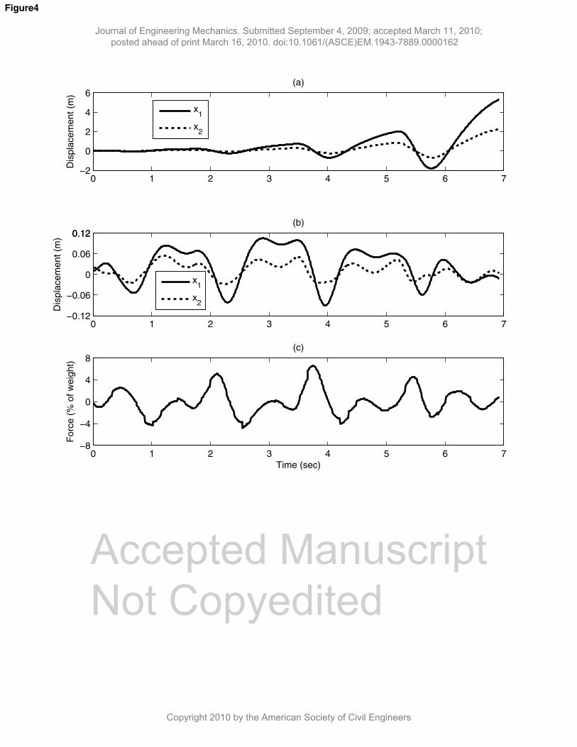
A harmonic base excitation of frequency 7.8 rad/sec (close to 2

n ) is applied to a

damped case of the 2DOF system considered previously for the free vibration study. The

damping parameters assumed are c1/m1 = c2/m2 =1. Fig. 4(a) shows that the responses of

the viscously damped 2DOF system diverge for the harmonic excitation considered. This

clearly happens due to the instability in the linear time-varying system which is

unexpected for linear viscously damped systems. The proposed controller is successful in

controlling the vibration within the first few seconds of the response (Fig. 4(b)) with

normalized control force requirement of less than 6.5% of the total weight (Fig. 4(c)).

The non-stationary random base acceleration is considered next. A band limited

excitation is simulated and modulated by a Shinozuka and Sato (1967) type of amplitude

modulating function (with parameters = 4, = 6.22 and = 3.11 leading to a peak of the

modulating function at around 4.99 s) to generate a transient, non-white, non-stationary

excitation. A plot of the simulated random excitation is shown in Fig. 5(a) with peak

acceleration close to 0.5g. To investigate the effect of damping and its effectiveness in

reducing the unstable response, the forced vibration responses of the 2DOF system with

damping coefficients c1/m1 = c2/m2 = 1 and c1/m1 = c2/m2 = 2 are studied and plotted in

Figs. 5(b) and 5(c) respectively. It is seen from Figs. 5(b) and 5(c) that even by doubling

the damping, the responses for both the states of the 2DOF system are uncontrollable.

Though for a higher viscous damping the build up of the responses are relatively delayed

as compared to the case with a lower damping, it is clearly unable to suppress the

instability (Fig. 5(c)).



Accep

ted M

anus

cript

Not Cop

yedit

ed

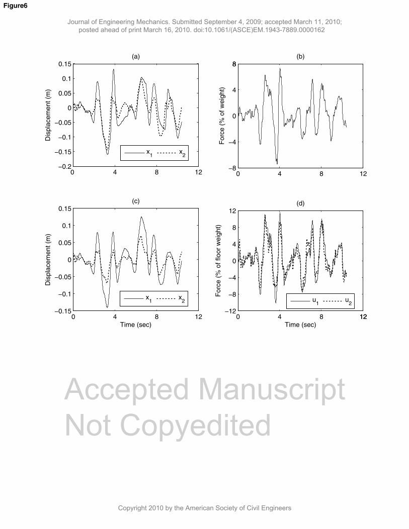
The proposed controller, with similar weights for the case of the previous controllers (R =

0.1, [Q]=[I] for frequency bands around 0 – 4 rad/sec; and R = 1, [Q]=[I] for the rest of

the frequencies), controls the responses as shown in Fig. 6(a) with peak control force

requirement of about 7.5% of the total weight (Fig. 6(b)).

In order to study the effect of multiple controllers in controlling response of the system,

two controllers located at the two degrees of freedom of the system are used instead of a

single controller applied to mass m1 as in the previous cases. The weighting matrices in

case of two controllers become R=0.1[I], [Q]=[I] for frequency bands around 0 – 4

rad/sec; and R=[I], [Q]=[I] for the rest of the frequency bands. The controlled

displacement responses and the control forces as a percentage of the weight of each floor

are plotted in Figs. 6(c) and 6(d) respectively. The controlled peak displacement

particularly for x2 (at the location where the second controller is placed) reduces

significantly by about 50% from about 0.15 m in the case of a single controller to about

0.07 m. Also, the peak control force for each of the controllers is much less than the peak

control force requirement for a single controller. The peak control forces for both the

controller are about 11.5% of the floor weight which amounts to about 4.7% of the total

weight in one controller and 6.7% of the total weight in the other (since mass ratio m1/m2

=0.7). However, it may be noted that the total energy consumed by the two controllers is

greater than that of a single controller, as the reduced controlled response and ease in

application with the avoidance of problems such as controller saturation comes at a price.



Accep

ted M

anus

cript

Not Cop

yedit

ed

Conclusions

A new type of controller for linear slowly time-varying systems which is based on the

multi-resolution capability of wavelet analysis to produce time-frequency signals is

proposed in this paper. The frequency dependent control gain matrices have been used

based on the desired emphasis to be placed on different frequency bands for controlling

the response of a system. An optimal control problem is formulated and is seen to follow

a LQR problem constrained to a band of frequency. The solution of this problem to

different frequency bands leads to a sub-optimal constrained solution. While the

flexibility of choosing frequency dependent weighting matrices provides versatility to the

control scheme, the synthesis of the control force in time domain by using linear

combination of filtered time-frequency signals weighted by frequency band dependent

gains accounts for evolutionary frequency content in a time varying system. The control

scheme uses filtered signals in time-frequency domain with the MRA based DWT aiding

the process through a fast numerical algorithm and hence is efficient for real-time

implementation.

The numerical studies carried out in this paper with the wavelet controller developed

using Daubechies wavelet have proved the efficiency of the controller. The proposed

controller has been shown to control response of linear time varying systems where the

conventional LQR controller has been unsuccessful. The application of the wavelet based

multi resolution controller to SDOF and MDOF linear time varying systems for both free

and forced vibrations (with harmonic and random excitations) has been successful in

efficiently suppressing instabilities even in cases where increased viscous damping has



Accep

ted M

anus

cript

Not Cop

yedit

ed

been ineffective. The developed controller in this paper holds promise for extension in

suppressing sub-harmonic and super-harmonic responses in non-linear systems and will

be addressed by the authors in forthcoming papers.

Acknowledgements

The financial support by Rice University and Trinity College Dublin for this research

work is gratefully acknowledged. This work was carried out during the visit of the first

author to Rice University.

The paper was submitted earlier to the date indicated, as the manuscript had to

be switched from the old system to the new online Editorial manager.



Accep

ted M

anus

cript

Not Cop

yedit

ed

References

Daubechies, I. (1992). Ten lectures on wavelets, Society of Industrial and Applied

Mathematics, Philadelphia.

Den Hartog, J.P. (1956). Mechanical vibrations, McGraw Hill, New York.

Dimentberg, M.F. (1988) Statistical dynamics of non-linear and linear time varying

systems, Wiley, New York.

Ibrahim, R.A. (1985) Parametric random vibration, Wiley, New York.

Ioannou P. and Sun, J. (1996).Robust Adaptive Control, Prentice Hall, New York (out of

print in 2003), electronic copy at

http://www-rcf.usc.edu/~ioannou/Robust_Adaptive_Control.htm

Kamen, E.W. (1988). “The poles and zeros of a linear time-varying system”, Linear

Algebra and Its Applications, 98, 263-289.

Shinozuka, M. and Sato, Y. (1967). “Simulation of nonstationary random processes”,

Journal of Engineering Mechanics, ASCE, 93(1), 11-40.

Sun, J. and Ioannou, P. (1992). “ Robust adaptive LQ control schemes”, IEEE Trans on

Automatic Control, 37(1), 100-106.

Tsakalis, K.S. and Ioannou, P. (1993). Linear time varying plants: Control and

adaptation, Prentice Hall, New York.



http://www-rcf.usc.edu/~ioannou/Robust_Adaptive_Control.htm

Accep

ted M

anus

cript

Not Cop

yedit

ed

List of Figures:

Fig. 1 2DOF system

Fig.2 (a) Uncontrolled response of SDOF system (b) Fourier amplitude of the

uncontrolled response (c) Comparison of controlled response for the LQR and the

wavelet controller (d) Control force for the LQR and the wavelet controller (e) Controlled

response for wavelet controller (longer duration) (f) Control force for wavelet controller

(longer duration) (g) Fourier amplitude of the control force for the wavelet controller

Fig. 3 (a) Free vibration response of 2DOF system (b) Fourier Amplitude of responses of

2DOF system (c) Controlled responses of 2DOF free vibration (d) Control force for

controlling free vibration

Fig. 4 Harmonic excitation of frequency 7.8 rad/sec with viscous damping (a)

Uncontrolled response (b) Controlled displacement responses (c) Control force for

harmonic excitation

Fig. 5 (a) Random nonstationary excitation simulated with amplitude modulation (b)

Responses of 2DOF damped system with c1/m1=c2/m2=1 (c) Responses of 2DOF damped

system with c1/m1= c2/m2 =2

Fig. 6(a) Controlled response with single controller (b) Control force with single

controller (c) Controlled response with two controllers (b) Control forces with two

controllers



c1 c2

m2 m1

x1(t) x2(t) k1(1+1)f1 k2(1+2)f2

Figure1

Accepted Manuscript Not Copyedited



0 5 10 15 2010

1

102

103

Frequency, ω (rad/s)

|X(ω

)|

(b)

0 2 4 6 8 10−15

−10

−5

0

5

Time (sec)

Dis

pla

ce

men

t (m

)

(a)

0 2 4 6 8 10−0.2

−0.1

0

0.1

0.2

Time (sec)

Dis

pla

ce

me

nt

(m)

(c)

0 2 4 6 8 10−8

−4

0

4

8

Time (sec)

Fo

rce

(%

of

we

igh

t)

(d)

LQR

wavelet

LQR

wavelet

Figure2a-d




0 5 10 15 20−0.01

−0.005

0

0.005

0.01

Time (sec)

Dis

pla

cem

ent

(m)

(e)

0 5 10 15 20−1

−0.5

0

0.5

1

1.5

2

Time (sec)

Forc

e (

% o

f w

eig

ht)

(f)

Figure2e-f




0 5 10 15 20 25 30 3510

−1

100

101

102


Fo

urie

r A

mp

litu

de

(g)

Figure2g




0 5 10 15 2010

1

102

103


Fourier

Am

plit

ude

(b)

0 2 4 6 8−2

0

2

4

6

Time (sec)

Dis

pla

cem

ent (m

)(a)

0 2 4 6 8−0.03

−0.02

−0.01

0

0.01

0.02

0.03

Time (sec)

Dis

pla

cm

ent (m

)

(c)

0 2 4 6 8−2

−1

0

1

2

3

4

Time (sec)

Forc

e (

% o

f w

eig

ht)

(d)

x1

x2

x1

x2

|X1(ω)|

|X2(ω)|

Figure3




0 1 2 3 4 5 6 7−2

0

2

4

6

Dis

pla

ce

me

nt

(m)

(a)

0 1 2 3 4 5 6 7−0.12

−0.06

0

0.06

0.120.12

Dis

pla

ce

me

nt

(m)

(b)

0 1 2 3 4 5 6 7−8

−4

0

4

8

Time (sec)

Fo

rce

(%

of

we

igh

t)

(c)

x1

x2

x1

x2

Figure4




0 2 4 6 8 10 12−5

0

5

Accele

ration (

m/s

2) (a)

0 2 4 6 8 10 12−30

−15

0

15

30

Dis

pla

cem

ent

(m) (b)

0 2 4 6 8 10 12−5

0

5

Time (sec)

Dis

pla

cem

ent

(m) (c)

x

1x

2

x1

x2

Figure5




0 4 8 12−0.2

−0.15

−0.1

−0.05

0

0.05

0.1

0.15

Dis

pla

cem

ent

(m)

(a)

0 4 8 12−8

−4

0

4

88

Forc

e (

% o

f w

eig

ht)

(b)

0 4 8 12−0.15

−0.1

−0.05

0

0.05

0.1

0.15

Time (sec)

Dis

pla

cem

ent

(m)

(c)

0 4 8 1212−12

−8

−4

0

4

8

12

Time (sec)

Forc

e (

% o

f floor

weig

ht)

(d)

x1

x2

x1

x2 u

1u

2

Figure6




a multi-scale wavelet- lqr controller for …nagaraja/j60.pdf · a multi-scale wavelet- lqr...

Documents