a multidimensional data model with...
TRANSCRIPT

A MULTIDIMENSIONAL DATA MODEL WITH SUBCATEGORIES
FOR EXPRESSING AND REPAIRING SUMMARIZABILITY
by
Sina Ariyan
A thesis submitted to
the Faculty of Graduate Studies and Research
in partial fulfillment of
the requirements for the degree of
DOCTOR OF PHILOSOPHY
School of Computer Science
at
CARLETON UNIVERSITY
Ottawa, Ontario
September, 2014
c⃝ Copyright by Sina Ariyan, 2014

Table of Contents
List of Figures v
Abstract vii
Acknowledgements viii
Chapter 1 Introduction 1
Chapter 2 Background and Literature Review 13
2.1 Multidimensional Databases . . . . . . . . . . . . . . . . . . . . . . . . . 13
2.2 MD Queries . . . . . . . . . . . . . . . . . . . . . . . . . . . . . . . . . . 14
2.2.1 MD Queries in SQL . . . . . . . . . . . . . . . . . . . . . . . . . 15
2.2.2 The MDX Query Language . . . . . . . . . . . . . . . . . . . . . 16
2.2.3 Datalog With Aggregation . . . . . . . . . . . . . . . . . . . . . . 17
2.3 Summarizability . . . . . . . . . . . . . . . . . . . . . . . . . . . . . . . . 18
2.4 Data Repairs of MDDBs . . . . . . . . . . . . . . . . . . . . . . . . . . . 20
2.5 Related Work: State of the Art . . . . . . . . . . . . . . . . . . . . . . . . 22
2.5.1 Multidimensional Data Models . . . . . . . . . . . . . . . . . . . 22
2.5.2 Summarizability . . . . . . . . . . . . . . . . . . . . . . . . . . . 24
2.5.3 Cube View Selection . . . . . . . . . . . . . . . . . . . . . . . . . 29
Chapter 3 Structural Repairs of Multidimensional Databases 31
3.1 Structural Repairs . . . . . . . . . . . . . . . . . . . . . . . . . . . . . . . 31
3.2 Properties of Structural Repairs . . . . . . . . . . . . . . . . . . . . . . . . 36
3.3 Virtual Repairs in MDX . . . . . . . . . . . . . . . . . . . . . . . . . . . . 40
3.4 Discussion . . . . . . . . . . . . . . . . . . . . . . . . . . . . . . . . . . . 42
Chapter 4 The Extended HM Model 45
4.1 The Multidimensional Model . . . . . . . . . . . . . . . . . . . . . . . . . 45
ii

4.2 Creating EHM Dimensions . . . . . . . . . . . . . . . . . . . . . . . . . . 48
4.2.1 The ADD-LINK Algorithm . . . . . . . . . . . . . . . . . . . . . 51
4.3 EHM and ROLAP schemas . . . . . . . . . . . . . . . . . . . . . . . . . . 54
Chapter 5 EHM and Summarizability 56
5.1 Flexible Summarizability for EHM . . . . . . . . . . . . . . . . . . . . . . 56
5.2 Computing Summarizability Sets in HM . . . . . . . . . . . . . . . . . . . 60
5.3 Computing Summarizability Sets in EHM . . . . . . . . . . . . . . . . . . 62
5.3.1 The COMPUTE-SUMSETS Algorithm . . . . . . . . . . . . . . . 64
5.4 EHM and Expressiveness . . . . . . . . . . . . . . . . . . . . . . . . . . . 68
Chapter 6 Query Answering 73
6.1 The Datalog Setting . . . . . . . . . . . . . . . . . . . . . . . . . . . . . . 73
6.2 MD Aggregate Queries . . . . . . . . . . . . . . . . . . . . . . . . . . . . 74
6.3 The Query Answering Problem . . . . . . . . . . . . . . . . . . . . . . . . 77
6.4 Query answering in EHM . . . . . . . . . . . . . . . . . . . . . . . . . . . 78
Chapter 7 Repairs of Non-Summarizable HM Dimensions 85
7.1 The EHM-based Repair Process . . . . . . . . . . . . . . . . . . . . . . . 85
7.2 Canonical Mapping: From HM to Compliant EHM Dimensions . . . . . . 86
7.2.1 The FIND-PCM Algorithm . . . . . . . . . . . . . . . . . . . . . 89
7.3 E-repairs . . . . . . . . . . . . . . . . . . . . . . . . . . . . . . . . . . . . 95
7.4 Discussion . . . . . . . . . . . . . . . . . . . . . . . . . . . . . . . . . . . 100
Chapter 8 Experiments 102
8.1 Introduction . . . . . . . . . . . . . . . . . . . . . . . . . . . . . . . . . . 102
8.2 Experimental Setting . . . . . . . . . . . . . . . . . . . . . . . . . . . . . 103
8.3 Creating HM Dimensions vs Finding Preferred Canonical Mappings . . . . 104
8.4 Query Answering Performance . . . . . . . . . . . . . . . . . . . . . . . . 107
Chapter 9 Conclusions and Future Work 115
9.1 Conclusions . . . . . . . . . . . . . . . . . . . . . . . . . . . . . . . . . . 115
iii

9.2 Future Work . . . . . . . . . . . . . . . . . . . . . . . . . . . . . . . . . . 117
Bibliography 119
iv

List of Figures
1.1 Sales database . . . . . . . . . . . . . . . . . . . . . . . . . . . . . 2
1.2 The Employee dimension: employees can have multiple parents . . 4
1.3 A summarizable yet not strictly-summarizable dimension . . . . . . 5
1.4 An EHM Location dimension . . . . . . . . . . . . . . . . . . . . 8
2.1 A minimal data repair for the Location dimension of Figure 1.1 . . 21
2.2 Data repairs of the Location dimension . . . . . . . . . . . . . . . 27
3.1 An SR for the Location dimension . . . . . . . . . . . . . . . . . 33
3.2 Another SR for the Location dimension . . . . . . . . . . . . . . . 33
3.3 Another minimal SR for the Location dimension . . . . . . . . . . 36
3.4 Structural repairs and non-strictness . . . . . . . . . . . . . . . . . 43
3.5 Combining structural repairs and data repairs . . . . . . . . . . . . . 44
4.1 Steps of the add link algorithm for creating the Location dimension 48
4.2 Star implementation of the Location EHM dimension . . . . . . . 55
5.1 An HM dimension with non-transitive summarizability sets . . . . . 61
6.1 The Location and Date EHM dimensions . . . . . . . . . . . . . . 75
7.1 Data vs EHM-based repairs (complexities are only in terms of in-
stance size) . . . . . . . . . . . . . . . . . . . . . . . . . . . . . . 86
7.2 A non-summarizable result of a canonical mapping for the Location
dimension . . . . . . . . . . . . . . . . . . . . . . . . . . . . . . . 87
7.3 A minimal e-repair for the compliant EHM instance of Figure 7.2 . . 96
8.1 Instance size vs dimension creation time (for small instances) . . . . 105
8.2 Instance size vs dimension creation time (for large instances) . . . . 106
8.3 The effect of adding categories on creation time . . . . . . . . . . . 108
8.4 HM schemas for dimensions Location, Date, Product and Employee109
v

8.5 Query answering time for selected queries . . . . . . . . . . . . . . 113
8.6 The impact of fact table size on query answering time . . . . . . . . 114
vi

Abstract
In multidimensional (MD) databases summarizability is a key property for obtaining in-
teractive response times. With summarizable dimensions, pre-computed and materialized
aggregate query results at lower levels of the dimension hierarchy can be used to correctly
compute results at higher levels of the same hierarchy, improving efficiency. Being summa-
rizability such a desirable property, we argue that established MD models cannot properly
model the summarizability condition, and this is a consequence of the limited expressive
power of the modeling languages. In addition, because of limitations in existing MD mod-
els, algorithms for deciding summarizability and cube view selection are not efficient or
practical.
We propose an extension to the Hurtado-Meldelzon (HM) MD model, the EHM model,
that includes subcategories and explore its properties specially in addressing issues related
to summarizability. We investigate the extended model as a way to directly model MD-
DBs, with some clear advantages over HM models. Most importantly, EHM is -in a precise
technical sense- more expressive than HM for modeling MDDBs that are subject to sum-
marizability conditions. Moreover, given an MD aggregate query in an EHM database, we
can determine in a practical way (that only requires processing the dimension schema as
opposed to the instance), from which minimal subset of pre-computed cube views it can be
correctly computed.
Our extended model allows for a repair approach that transforms non-summarizable
HM dimensions into summarizable EHM dimensions. We propose and formalize a two-
step process that involves modifying both the schema and the instance of a non-summarizable
HM dimension.
vii

Acknowledgements
First, I offer my sincerest gratitude to my supervisor, Professor Leopoldo Bertossi, for his
guidance throughout this research. He has supported and encouraged me with his knowl-
edge and patience. He has a been a true professional. The work presented in this thesis
would not have been possible without his advice and support.
I would like to thank members of my PhD proposal and thesis committees Dr. Illuju
Kiringa and Dr. Douglas Howe, and members of my comprehensive examination commit-
tee, Dr. Carlisle Adams and Dr. Jean-Pierre Corriveau.
I dedicate this thesis to my mother. Making you happy and proud has always been my
motivation. You have always supported me and never asked for anything in return. From
the deepest part of my heart, I love you and I will always miss you.
viii

Chapter 1
Introduction
On-Line Analytical Processing (OLAP) was a notion introduced by Codd [24] to character-
ize a set of requirements for consolidating, viewing and analyzing data organized according
to the multidimensional data model (MDM). In recent years, OLAP has become one of the
central issues in database research, and OLAP technologies have become important appli-
cations in the database industry.
A multidimensional database (MDDB) is an implementation of a multidimensional data
model. It combines data from different sources, for analysis and decision support. MDDBs
represent data in terms of dimensions and fact tables. Dimensions themselves are usually
graphs, and their structure defines the levels of detail at which data can be summarized for
visualization and manipulation.
In an MDM, a dimension is modeled by two hierarchies: a dimension schema and a
dimension instance. A dimension schema is a hierarchy composed of a number of levels
or categories, each of which represents a different level of granularity. Instantiating the di-
mension schema by values at each level forms the dimension instance and creates another
hierarchy parallel to the category hierarchy. A row in the fact table corresponds to a mea-
surement that is taken at the intersection of the categories at the bottom of the dimensions:
a quantity that is given context through base dimension values.
This MD organization allows users to aggregate data at different levels of granularity,
corresponding to different levels of categories in the hierarchies. Aggregation is the most
important operation in OLAP applications. OLAP queries are complex, may involve mas-
sive data, and also aggregation. Therefore, fast query answering is a crucial task in OLAP
[46].
Some models of MDDBs have been proposed in the literature [3, 17, 31, 45, 47, 59,
60, 71], ranging from simple cube models that view data as n-dimensional cubes, to hi-
erarchical models that explicitly capture the structural relationship between categories in
1

2
(a) Location schema (b) Location instance (c) Fact table
Figure 1.1: Sales database
the dimensions. We have adopted as basis for our research the Hurtado-Mendelzon (HM)
model of MDDBs [37, 41]. It is an established and extensively investigated model, and it
provides solid and clear foundations for further investigation on MDDBs.
Example 1 We represent data about a company sales for different times and locations in
Figure 1.1. We illustrate there only the Location dimension, represented as a hierarchy
of places where the company has branches. The Location dimension schema is in Figure
1.1a, and a possible instance for it is shown in Figure 1.1b.
In this schema, City, State, etc., are categories. Country is a parent of categories
State and Province; and an ancestor of category City. Category City is a base category,
i.e. it has no children. At the instance level, element LA of City rolls up to USA, as an
ancestor element in category Country. LA and Vancouver are base elements. As we can
see, both the schema and the instance are endowed each with compatible partial orders
(lattices) that are directed from the bottom to the top.
Figure 1.1c shows the fact table containing data about sales for cities (of the base cat-
egory) at different times. Here, Sales is the single measure attribute of the fact table.
�
The hierarchical structure of a dimension schema allows us to derive the results of
aggregate queries posed on non-base (i.e. higher level) categories directly from the fact
table. However, due to the possibly very large volumes of data in MDDBs, computation
from scratch of aggregate queries should be avoided whenever possible. Ideally, aggregate
query results at lower levels (i.e. more detailed, pre-computed views of data) should be
used to correctly calculate results at higher levels of the hierarchy (i.e. less detailed views

3
of data). As an example, for the instance in Figure 1.1b, it is always possible to compute
sales values for different continents directly from the fact table. However, if possible, it
is more practical to derive the results by aggregating over pre-computed sales values for
one (or a combination) of categories from a level higher than City (in this case one of
categories Country, State or Province or a combination of these categories). For this
derivation to happen correctly, every base element that rolls up to some element in the
parent category must pass through one and only one element from the ancestor categories
[41]. If this is the case for all higher level categories, we say that the dimension instance is
summarizable.
Summarizability can be defined as the ability of an aggregate query to correctly com-
pute a cube view from another cube view where both cube views are defined in a single
dimension. This notion can be applied to an instance in local terms: if a parent category
and a set of its descendant categories allow for this correct derivation, we say that the parent
is (locally) summarizable from those descendants. As an example, category All is sum-
marizable from Continent, but Country is not summarizable from Province: the base
elements LA and London do not pass through any element from Province when rolling up
to Country. Also, category Continent is not summarizable from Country because ele-
ment London rolls up to element Europe from more than one path (once through England
and once through UK). In the absence of summarizability, a multidimensional database will
either return incorrect query results when using pre-computed views, or lose efficiency by
having to compute the answers from scratch [42, 53].
It is worth noting that in our Location dimension example, the issue of multiple par-
ents could have been avoided in the ETL phase of data warehouse design. However, in
some cases we actually need multiple parents (or ancestors) for an element in a single up-
per level dimension. The Employee dimension of Figure 1.2 is such an example. Some
employees (shown in red) are supervised by more than one manager. Therefore, having
multiple parents should be allowed and cannot be avoided even in the ETL phase.
Global summarizability (i.e. summarizability of a dimension) can be defined in one
of two ways: relative to all the descendants of a category or only to a subclass of them.
Accordingly, we say that a dimension is strictly-summarizable if every category is (locally)
summarizable from each one of its descendant categories. This is the concept that has been

4
Figure 1.2: The Employee dimension: employees can have multiple parents
the focus of previous research in the literature [13, 15, 20, 21, 41, 72]. In particular, it
has been established that for a dimension to be strictly-summarizable, it must satisfy three
conditions [42, 72]:
1. The dimension schema must have a single base category, which contains all the
elements that have no children.
2. The dimension instance must be strict, i.e. each element in a category must have at
most one parent in each upper category.
3. The instance has to be homogeneous (aka. covering), i.e. each element in a category
has at least one parent element in each parent category.
The last two conditions can be seen as semantic constraints on a dimension instance. Di-
mensions that do not satisfy strictness or homogeneity (or both) are said to be inconsistent.
The Location dimension instance in Figure 1.1 has a single base category, City, but it is
inconsistent. The instance violates strictness: London rolls up to the two different elements
in Country: England and UK. It is also non-homogeneous, i.e. heterogeneous: London
does not roll up to any element in State or Province. Dimensions may become incon-
sistent for several reasons, in particular, as the result of a poor design or a series of update
operations [44].
Notice above that for dimensions with multiple base categories, homogeneity and strict-
ness does not necessarily guaranty summarizability. Dimensions with multiple base cate-
gories can be useful when/if a single column of the fact table needs to refer to elements
of multiple different categories (e.g. a case where employees and managers can both sell
products). However this is not very common in practice.

5
Figure 1.3: A summarizable yet not strictly-summarizable dimension
We refer to the combination of these three conditions as the strict-summarizability con-
ditions. We argue that the strict-summarizability conditions are too restrictive, and impos-
ing them will filter out a wide range of useful models and instances. This includes any
dimension that has multiple base categories. However, there are other cases. As another
example, the instance in Figure 1.3 shows that aggregate results for category Country can-
not be derived from State, nor from Province. Therefore, the dimension is not strictly-
summarizable. However, Country is summarizable from the combination of State and
Province. Therefore, we can still take advantage of pre-computed cube views at the level
of State and Province to compute aggregate results for Country. We will redefine the
notion of summarizability for a dimension instance to take multi-child aggregation into
consideration.
The restrictions imposed by strict-summarizability are not the whole problem. It is not
only that an instance at hand fails to be summarizable. Actually, there are many commonly
used dimensions for which the HM metamodel (i.e. the framework that supports the cre-
ation of specific HM models) fails to accommodate an MD model, including instances, that
satisfies summarizability. This is because any HM model that captures the external reality
will be bound, already by the sheer MD schema used, to have instances that do not satisfy
the summarizability conditions expressed above. An example is given by Figure 1.3: when
capturing in an HM model a real-world assumption, such as having State and Province,
at the same level, as immediate and partitioning ancestors of City, there is no HM model
that can capture this domain in a summarizable way. Every reasonable instance (e.g. with
non-empty categories) will not be summarizable.

6
One way to approach the problem of modeling such domains consists in making changes
to the dimension schema and/or the dimension instance to restore strictness and homo-
geneity. In accordance with the area of repairs and consistent query answering (CQA) in
relational databases [7, 11, 12], a resulting dimension instance could be called a repair
of the original one. A minimal repair is one that minimally differs (in some prescribed
sense of minimality) from the original dimension and satisfies strictness and homogeneity
[9, 13, 72]. As expected, minimality can be defined and characterized in different ways
[11].
Previous work on repairing MDDBs has focused mainly on changing the dimension in-
stance by modifying data elements or links between them [13, 15, 20, 19, 72]. Repairs ob-
tained in this way are called data repairs. These repairs have been proposed to deal mainly
with non-strictness, and usually assuming homogeneity [13, 19]. When both non-strictness
and heterogeneity are addressed [15, 20, 72], the latter has been confronted through the
insertion of null values [40, 65, 72]. There exist real world domains, such as the one in
Example 1, where this approach may produce an unnatural solution, e.g. for the instance
in Figure 1.1b), one that connects London to California in State, and to BC or a null
in Province. The process leads to an unnatural repair, that does not quite conform to the
external reality. Of course, additional restrictions could be imposed on the repair process,
like not allowing such links, but in some cases there might be no repair then.
In some cases, inconsistency may be caused by a problematic dimension schema. There-
fore, changing the dimension instance may be only a temporary solution. Future update
operations will probably produce new inconsistencies. So, exploring and considering struc-
tural changes, i.e. changes in the schema, is a natural way to go. This is an idea that has
been suggested in [40], to overcome heterogeneity. In [9], we introduced and investigated
the notion of structural repair, as an alternative to data repair. They modify the schema of
an inconsistent dimension, to restore strictness and homogeneity.
Structural repairs restrict changes to dimension instances by allowing changes that af-
fect only the category lattice and the distribution of the data elements in different categories.
In particular, there are no “data changes” (as in data repairs), in the sense that the data el-
ements and also the edges between them remain. In the case of a ROLAP data warehouse

7
(with relational schemas, like star or snow flake) fewer data changes on a dimension in-
stance directly results in fewer changes on records in the underlying database.
With data repairs, a single change on a dimension instance directly results in several
changes on records in the underlying relational database (the number of changes depends
on the underlying ROLAP schema, and is usually larger when changes are made at higher
levels of the instance [72]). With structural repairs this is not the case, which is advanta-
geous for users who do not want their records changed. On the other hand, with structural
repairs, some sort of query reformulation becomes necessary since old queries may refer
to categories of the old schema that may have changed or disappeared (with consequent
changes on the relational schemas).
In this thesis, as an alternative to repairs for confronting the modeling problem men-
tioned above, we introduce and investigate an extension of the HM metamodel (Section
4.1). This extension allows us to produce extended HM (EHM) models. The main ingredi-
ent of this extension is the addition of subcategories. Figure 1.4 shows an EHM model of
the Location dimension. Subcategories are shown as rectangles inside a category (when
a subcategory coincides with its containing category, we omit the inner rectangle). The
idea, that we develop in this work, is that, by introducing subcategories Country1 and
Country2, category Continent now becomes summarizable from its direct lower level, in
this case from subcategory Country1. We did not have summarizability in any HM model
of this dimension.
We investigate the extended model as a way to directly model MDDBs, with some clear
advantages over HM models. Most importantly, EHM is -in a precise technical sense- more
expressive than HM for modeling MDDBs subject to summarizability conditions. In partic-
ular, it follows that a summarizable HM model is still a summarizable EHM model, without
any changes. Also, there are common real-world examples for which no summarizable HM
model exists, but can be modeled using a summarizable EHM model.
Compared to arbitrary HM models, EHM models have a positive computational feature:
Given a category, one can decide whether it is (locally) summarizable from an arbitrary
subset of its descendants without having to process the dimension instance (which is usually
very large). Furthermore, this decision algorithm can be extended in order to compute the
class of all subsets of descendants from which the category is summarizable. EHM models

8
Figure 1.4: An EHM Location dimension
enjoy this feature because subcategories reflect the exact structure of the dimension instance
(but at a much higher level or granularity, which reduces size). As expected, this behavior
comes at the expense of imposing additional semantic constraints on dimension instances.
This will have an impact on the population and maintenance of the dimension instance.
However, this cost is more than offset by the benefits for OLAP query answering. More
precisely, when confronted with an aggregate query Q, it will be possible to determine (at
a preprocessing step) the most appropriate set of pre-computed aggregate views at lower
levels that can be used to efficiently answer Q.
Notice that, for an arbitrary, non-extended HM model, a decision procedure and an al-
gorithm for computing “summarizable classes of children” as for EHM models will also
depend on the dimension instance, which is usually very large. Therefore, a similar prepro-
cessing step becomes impractical for aggregate query answering in HM models. It should
be noted that although the EHM metamodel is an extension of the HM metamodel, not
necessarily an HM dimension (including the schema and instance) is an EHM dimension,
because the latter are subject to additional conditions, namely roll-up relations between
pairs of subcategories must be total functions. As a consequence, the algorithms for the
EHM model just described do not necessarily apply to HM models, as expected.
The semantic conditions on subcategories of EHM dimension instances (i.e. the con-
dition of roll-up relations being total functions) have to be enforced and maintained. We
provide an algorithm for populating a EHM dimension instance. It is based on first speci-
fying the categories, and then adding data links one by one. In some cases that seem to be
rare in practice, this may require updating the subcategory schema. More precisely, split-
ting a subcategory in two (within the same category), and creating a new link to the upper

9
subcategories. Actually, this approach opens the possibility of creating EHM models from
scratch which we also investigate in Section 4.2.
We show that the extended HM model does not produce complications with the im-
plementation of MDDBs as/on relational databases (ROLAP) [48]. Actually, our extended
HM models can be captured by the well-known and familiar ROLAP schemas, like star or
snowflake, with minor modifications.
We address query answering in a multidimensional setting with EHM models. Intu-
itively, the query answering problem is, given an MD database, an aggregate query and a
set of pre-computed cube views, to find another query (i.e. a rewriting) that produces the
same results using the pre-computed cube views.
The subcategory structure of a set of EHM dimensions provides an important feature
which is to specialize a cube view to selected subcategories. This feature allows us to derive
the result of an aggregate query by combining a subset of cube views that are specialized
to selected subcategories. We show that finding such a selection of specialized cube views
can be done efficiently for EHM dimensions (without processing dimension instances).
The EHM model allows for a repair approach that transforms non-summarizable HM
dimensions into summarizable EHM dimensions. We propose a two-step process that in-
volves modifying both the schema and the instance of an inconsistent HM dimension.
First, by the addition of subcategories, an inconsistent HM instance is transformed into
an EHM instance through a process called canonical mapping (CM). A CM result contains
the same set of categories, and the same elements and links in the dimension instance,
but adds new subcategories and links between them in the schema. A preferred canonical
mapping (PCM) is one that minimizes the redistribution of elements in new subcategories.
We will show that such minimization helps avoid potential future joins within queries for
recombining elements of a category, thus improving query answering performance.
We provide an algorithm that, given an inconsistent HM instance, produces one of the
possible PCMs. In theory, exponentially many PCMs may exist for an HM instance. Our
algorithm chooses only one of those candidates in polynomial time with regards to the HM
instance size. We can decide in polynomial time whether a compliant EHM instance is a
PCM of an inconsistent HM instance. In most cases, the PCM that is the result of the first
step is summarizable. If this is not the case, another set of (instance-based) changes need

10
to be applied to enforce summarizability.
In the second step of the repair process, changes are applied to links in the dimension
instance of a chosen PCM to enforce summarizability, resulting in a so-called e-repair. As
before, we tend to minimize link changes within the dimension instance, the result being
a minimal e-repair. We will show that all minimal e-repairs of a PCM (or more generally,
of a compliant EHM instance) can be found without the need to process the dimension
instance.
Comparing the EHM-based repair process described above with the usual data repair
approach presented in [13, 15, 20, 19], the former incurs in lower computational cost for
restoring summarizability of an inconsistent HM instance. In [20], it is shown that the
problem of computing a minimal data repair is NP-hard(as opposed to the EHM-repair
process which is P-TIME) with regard to instance size. In addition, we show that the result
of the EHM-based repair process is more natural compared to the data and structural repair
approaches.
The main focus of our research has been on creating summarizable dimensions either
from scratch or by modifying existing non-summarizable HM models. Consequently, we
can take advantage of the benefits of summarizability with regards to query answering. The
contributions of this dissertation can be summarized as follows:
1. We explore and investigate structural repairs as an alternative to data repairs. They
modify the schema of an inconsistent dimension, to restore strictness and homogene-
ity. We establish that under certain conditions, a structural repair reduces the cost
wrt changing the dimension instance. We also show how query-scoped calculated
members in MDX can be used to create virtual repairs that simulate structural re-
pairs. Investigating the properties of this schema-based repair approach becomes a
basis for the development of our extended model (Chapter 3).
2. We introduce and formalize the Extended HM models (EHM models) for MDDBs.
Categories and links are still the user-defined ingredients of an EHM schema. How-
ever, subcategories are an additional ingredient that, if structured properly within
categories of an EHM schema, enforce summarizability and provide the subsequent
benefits. We also specify when an HM model can be considered as a particular kind
of EHM model (Chapter 4).

11
3. We show how EHM dimension instances can be populated from scratch (Section 4.2).
We propose the ADD-LINK algorithm that takes categories (but not subcategories)
as user-defined inputs. Data elements can then be added one by one opening the
possibility of incrementally creating EHM models from scratch.
4. We show that EHM models can be implemented with the usual ROLAP schemas,
with minor modifications. Additional tables will be added corresponding to cate-
gories that contain more than one subcategory (Section 4.3).
5. We propose a new, less restrictive notion of summarizability that applies to both HM
and EHM dimensions (Section 5.1). We show that: (a) Summarizable HM models
are still summarizable as EHM models. (b) There are sensible real-world examples
for which no summarizable HM model exists, but that can be modeled using a sum-
marizable EHM model, showing a difference in expressive power, between the HM
and EHM models.
6. We propose the COMPUTE-SUMSETS algorithm to determine from which pre-
computed cube views a cube view (i.e. aggregate query) can be correctly computed.
We show that this problem can be solved for EHM models with less computational
cost compared to arbitrary HM models (Section 5.3).
7. We provide a formal characterization of expressiveness for classes of dimension
models. We establish that the class of summarizable HM dimensions is less ex-
pressive than that of summarizable EHM dimensions (Section 5.4).
8. We formalize the problem of query answering using pre-computed cube views in an
MD setting. We show that, given a set of materialized pre-computed cube views in
an EHM setting, we can effectively rewrite new queries in terms of available views
and obtain query answers with better performance (Chapter 6).
9. We introduce and investigate an EHM-based repair approach that transforms non-
summarizable HM dimensions into summarizable EHM dimensions. We provide
the FIND-PCM algorithm that, given an arbitrary HM instance, generates an EHM
instance with the same set of categories and the same set of elements and links in
the dimension instance. We also show how summarizability can be guarantied by

12
modifying links in the dimension instance. We also analyze the complexity of this
approach and compare it to that of the traditional data repair approach on HM in-
stances (Chapter 7).
10. Finally, we show results of our experiments. Specifically, we have investigated,
through experiments, how much time it takes to create an MD database comprised of
EHM dimensions in comparison with that of a database containing HM dimensions.
We have experimented with a wide range of dimension sizes as well as different fact
table sizes. In addition, our experiments will show how query answering perfor-
mance is affected by the introduction of subcategories in EHM dimensions (Chapter
8).
It is worth noting that in the life cycle of a data warehouse, the extended model will ap-
pear in the design phase. However, the changes will not be manual, in the sense that the
users will not need to provide additional information to create and maintain subcategories.
Instead, the subcategory structure can be maintained automatically using our creation al-
gorithms. Of course, the performance improvements of these design changes will appear
in the query answering phase.

Chapter 2
Background and Literature Review
2.1 Multidimensional Databases
A multidimensional database (MDDB) is a data repository that provides an integrated en-
vironment for decision support queries that require complex aggregations on huge amounts
of data [10]. A model representing an MDDB is composed of logical cubes, facts and
dimensions.
A data cube is a data structure that allows fast analysis of data. It can also be defined as
the capability of manipulating and analyzing data from multiple perspectives. The arrange-
ment of data into cubes in MDMs overcomes some limitations of relational databases. A
data cube consists of numeric facts called measures which are categorized by dimensions.
Facts are measures assigned to instances of dimensions. They are typically numeric and
additive. Measures populate cells of a logical cube with the facts collected about business
operations.
In order to measure the facts at different granularity levels, a dimension is usually repre-
sented as a hierarchy of categories. The hierarchical structure allows the user to study facts
at different levels of detail. They provide structured labeling information to, otherwise
unordered, numeric measures.
Various MD models have been proposed and investigated in the literature [27, 30, 31,
48, 3, 18, 28, 43, 47, 51, 59, 66, 71]. Each model imposes different structural and semantic
conditions on the hierarchy of categories. In the simplest case, the hierarchy has a linear
form, i.e. every category is connected to at most one parent category and at most one child
category. More advanced models represent the hierarchy of categories using complex graph
structures such as lattices. We adopt as basis for our research the Hurtado-Mendelzon (HM)
model of MDDBs [37, 41] (for an overview of other MD models see Section 2.5.1).
In the HM model, a dimension schema S is a tuple of the form ⟨U, C,↗⟩, where U is
a possibly infinite set (the underlying data domain), C is a finite set of categories (or better,
13
14
category names), ⟨C,↗⟩ is a directed acyclic graph. Notice that ↗ is a binary relation
between categories. Its transitive and reflexive closure is denoted by↗∗.
Every dimension schema has a distinguished top category, All, which is reachable from
every other category: For every category c ∈ C, c ↗∗ All holds. Categories that have no
descendants are called base categories.
Given a dimension schema S, a dimension instance for the schema S is a tuple D =
⟨M, δ, <⟩, where M is the finite subset of U , δ : M → C is a total function (assigning
data elements to categories), and < is a binary relation onM that parallels relation↗ on
categories: e1 < e2 iff δ(e1) ↗ δ(e2). Element all ∈ M is the only element of category
All.
The transitive and reflexive closure of < is denoted with <∗, and can be used to define
the roll-up relations for any pair of categories ci, cj:
Rcjci (D) = {(ei, ej) | ei ∈ ci, ej ∈ cj, and ei <
∗ ej}.A fact table consists of a granularity and a measure. Measures are formalized by a set of
variables. Each variable has its specific domain of values. A base fact table (usually for
simplicity referred to as fact table) is the one, in which all of the categories in the granularity
are base categories of their corresponding dimension schema.
2.2 MD Queries
The most common aggregate queries in DWHs are those that perform grouping by the
values of a set of categories from different dimension schemas (known as a granularity),
and return a single aggregate value per group. These aggregate queries are known as cube
views [38]. The aggregation is achieved by upward navigation from base categories through
a path in the dimension schema, which is captured by roll-up relations.
Cube views are defined using distributive aggregate functions [32], with SUM, MAX
and MIN being the most common cases. We will use Ψf [c1, ..., cn] to denote a cube view at
granularity {c1, ..., cn} where f is the distributive aggregate function, and each ci is a cat-
egory (name) from a dimension schema Si. When we concentrate on a single dimension,
the cube view will be of the form Ψf [c], with c a category of a dimension schema S.
Lets assume D1, ..., Dn are a set of HM dimensions with schemas S1, ..., Sn and base
categories b1, ..., bn, respectively. Cube view Ψf [c1, ..., cn], where ck is a category from

15
schema Sk, can be defined as follows:
Πc1,...,cn,f(m)(Rc1b1(D1) ◃▹ ... ◃▹ Rcn
bn(Dn) ◃▹ F ) (2.1)
where m is a measure from fact table F .
Example 2 For an MD schema comprised of Location and Date dimensions, cube view
ΨSUM [State, Year] is defined as follows:
ΠState,Year,SUM(Sales)(RStateCity (Loc) ◃▹ RYear
Day (Dn) ◃▹ F ) (2.2)
where fact table F associates measure Sales to cities by day. �
2.2.1 MD Queries in SQL
MD queries can be expressed using SQL aggregate queries of the following form:
SELECT cj , . . . , cn, f(a) FROM T, Ri, . . . , Rm
WHERE conditions GROUP BY cj , . . . , cn
Here cj , . . . , cn are attributes (categories) of the roll-up relations Ri, . . . , Rm (treated as
tables), and f is one of min, max, count, sum, avg, applied to fact measure a.
This form of aggregation using SQL assumes a relational representation of the database
in which MDDBs are usually represented as a star or snowflake database [48], although
other relational representations have also been investigated [72].
Example 3 Assuming we have the following star representation of the Sales database
(with the dimension table of Location on the left, the fact table on the right and skipping
the representation of the dimension table for Date):
(LocationStar) (FactTable)
City State Province Country Continent All
LA California null US NA all
Vancouver null BC Canada NA all
Ottawa null ON Canada NA all
London null null England Europe all
London null null UK Europe all
City Date Sales
Ottawa Jan 1,14 6000
Vancouver Jan 1,14 4500
LA Jan 1,14 10000
Ottawa Jan 2,14 5500
Vancouver Jan 3,14 1400
Ottawa Jan 3,14 3000
The following SQL query returns total sales for different countries:

16
SELECT R.Country, SUM(F.Sales)
FROM FactTable F, RCountryCity R
WHERE F.City = R.City
GROUP BY R.Country
Notice that in the case of star schema,RCountryCity can simply be replaced by LocationStar
in the query. however, in the case of snowflake schema, it should be computed (as an inner
query) with a join operation over dimension tables. �
2.2.2 The MDX Query Language
MultiDimensional Expressions (MDX) [61, 69] is a declarative query language for multidi-
mensional databases designed by Microsoft. Results of MDX queries come back to client
programs as data structures that need to be further processed to look like a spreadsheet.
This is similar to how SQL works with relational databases.
Example 4 (example 3 continued) The following MDX query returns total sales for dif-
ferent countries:
SELECT [Measures].[Sales] ON COLUMNS,
[Location].[Country].CHILDREN ON ROWS
FROM [Sales]
Here, Sales represents the base cube view (i.e. fact table). �
An MDX query consists of axis specifications and a cube specification. It may also
contain an optional slicer specification that is used to define the slice of the cube to be
viewed. A simple MDX statement has the following form:
SELECT <axis specification> [,<axis specification>,...]
FROM <cube_specification>
WHERE <slicer_specification>
We can break this query down into pieces:

17
1. The SELECT clause defines the axes for the MDX query structure by identifying
data elements to include on each axis. MDX has several ways to do this. The basic
possibilities are to identify data elements either by choosing members of a category
or by specifying their parent element.
2. The FROM clause names the cube from which the data is being queried. This is
similar to the FROM clause of SQL that specifies the tables from which data is being
queried
3. The WHERE clause provides a place to specify members for other cube dimensions
that do not appear in the axes and filters data based on the conditions that are pro-
vided. The use of WHERE is optional. It is used when measures are not queried in
axis specifications (For simplicity, in the remaining sections we will skip the WHERE
clause and include measures in our axis specifications).
Example 5 We can write a simple MDX query that returns dollar and unit sales for quarters
of 2014 as follows:
SELECT {[Measures].[Dollar Sales],[Measures].[Unit Sales]}
ON COLUMNS,
{[Time].[2014].CHILDREN}ON ROWS
FROM [Sales]
Dollar Sales Unit Sales
Q1,2014 1,213,380.0 2,725
Q2,2014 855,600.0 2,100
Q3,2014 1,160,419.0 2,518
Q4,2014 1,638,560.0 3,122
2.2.3 Datalog With Aggregation
Datalog is a declarative logic programming language that is often used as a query language
for deductive databases. It has a simple uniform syntax to express relational queries and
to extend relational calculus with recursion. Datalog’s simplicity in expressing complex
queries has made it a viable choice for the formal representation of problems related to
data management and query processing.
A datalog rule is an expression of the form R1(u1) ← R2(u2), . . . , Rn(un) where
n ≥ 1, R1, . . . , Rn are relation names and u1, . . . , un are free tuples of appropriate

18
arities. Each variable occurring in u1 must occur in at least one of u2, . . . , un. A datalog
program is a finite set of datalog rules [1].
A datalog program defines the relations that occur in heads of rules based on other re-
lations. The definition is recursive, so defined relations can also occur in bodies of rules.
Thus a datalog program is interpreted as a mapping from instances over the relations oc-
curring in the bodies only, to instances over the relations occurring in the heads [1].
Different extensions of Datalog have been proposed to support aggregate rules [2, 4,
25, 29]. In [25], aggregate rules take the form P (a, x, Agg(u)) ← B(y), where P is
the answer collecting predicate, the body B(y) represents a conjunction of literals all of
whose variables are among those in y, a is a list of constants, x ∪ u ⊆ y, and Agg is an
aggregate operator such as Count or Sum. The variables x are the group-by variables.
That is, for each fixed value b for x, aggregation is performed over all tuples that make
B xb, the instantiation of B on b for x, true. Count(u) counts the number of distinct values
of u, while Sum(u) sums over all u, whether distinct or not. In Chapter 6, based on
the semantics proposed in [25] for Datalog with aggregation, we will formalize the query
answering problem in EHM.
Example 6 (example 3 continued) The following Datalog with aggregation query com-
putes total sales for different countries:
Q(ctr, Sum(sales)) ← F (cty, day, sales),RCountryCity (cty, ctr)
Here, F is a relation that represents the fact table. �
2.3 Summarizability
A common technique for speeding up OLAP query processing is to pre-compute some cube
views and use them for the derivation (or answering) of other cube views. This approach to
query answering is correct under the summarizability property, which ensures that higher-
level cube views (from the base categories and fact tables) can be correctly computed using
cube-views at lower level as if they were fact tables [43]. As shown in Example 7, the
reuse of pre-computed cube views has a great impact on query answering performance.
Therefore, maximizing summarizability between categories is a crucial optimization task
for MDDBs [46].

19
Example 7 Lets assume the Sales database of Figure 1.1 belongs to a worldwide corpo-
ration. The managers of this corporation need to compute its aggregate sales information
for every continent between the years 2003 and 2012.
Computing this query directly (i.e. without taking advantage of summarizability) re-
quires a join between three relations: RContinentCity , RYear
Day and the fact table. Assuming the
fact table contains daily values for 3000 cities over this period of time, these relations will
contain more than 3000, 3600 and 107 tuples respectively. Obviously this will be a time
consuming query.
On the other hand, if we were to compute the same query using a pre-computed cube
view, for example Ψsum[Country, Year], relations that were involved in the new join would
be RContinentCountry , RYear
Month and Ψsum[Country, Year] with at most 200, 120 and 24000 tuples
respectively. Hence, great improvement in query processing time would be obtained.
This performance improvement would be much more significant in real world examples
involving more than two dimensions (e.g. by adding a product dimension) and more de-
tailed base categories (e.g. a Location dimension with Branch as the base category rather
than City). �
As stated earlier, Reusing cube views is one the important features of multidimensional
databases. The following query (Lets call it CV c1,...,cn) shows a template for writing cube
views in MDX (for simplicity, some features of MDX that are irrelevant to our discussions
have been dropped in this template):
SELECT [Measures].MEMBERS ON AXIS(0),
{[c1].MEMBERS | [c1].[e1].CHILDREN} ON AXIS(1),...
{[cn].MEMBERS | [cn].[en].CHILDREN} ON AXIS(n)
FROM [base_cube]
Here, c1, ..., cn are categories (possibly from different dimensions), [ck].MEMBERS re-
trieves all elements that belong to category ck ([Measures].MEMBERS retrieves fact
measures), [ck].[ek].CHILDREN retrieves children of element ek from category ck,
and base cube is a cube generated by selecting base categories of different dimensions
(i.e. the fact table).

20
The following query template can be used to derive cube view CV c′1,...,c′n from another
pre-computed cube view CV c1,...,cn in MDX:
SELECT [Measures].MEMBERS ON AXIS(0),
{[c’1].MEMBERS | [c’1].[e1].CHILDREN} ON AXIS(1),...
{[c’n].MEMBERS | [c’n].[en].CHILDREN} ON AXIS(n)
FROM [CVc1,...,cn]
where c1, ..., cn, c′1, ..., c′n are categories from different dimensions and every c′i is an ances-
tor of ci.
An HM instance is considered to be summarizable if a cube view on any category c
can be computed a from pre-computed cube view for each one of its descendant categories
c′ (as if the cube view for c′ were a fact table) [13, 15, 20, 21, 41, 72]. We will refer to
this notion of summarizability (i.e. the one used in the literature) as strict-summarizability,
as we indicated in Chapter 1. The reason for this is that in Section 5.1 we will relax this
notion, providing a less restrictive definition of summarizability.
Definition 1 [72] An HM instance D is (a) Strict iff for all categories ci,cj , the roll-up
relation Rcjci (D) is a (possibly partial) function. (b) Homogeneous iff for all categories
ci,cj , the roll-up relation Rcjci (D) is total. (c) Consistent iff it satisfies the two previous
conditions; and inconsistent otherwise. �
Theorem 1 [41] An HM instance with a single base category is strictly-summarizable iff
it is consistent. �
2.4 Data Repairs of MDDBs
Data repairs have been introduced and studied in [13, 15, 19, 20, 72], and in some sense,
but not as repairs, in [40, 65]. In this case, changes are made to the instance (as opposed
to the schema) of an inconsistent dimension to restore consistency. In the following defini-
tion, dist(D,D′) denotes the symmetric difference between the sets of links in instances of
dimensions D and D′, i.e. dist(D,D′) = (<D \ <D′) ∪ (<D′ \ <D).

21
Figure 2.1: A minimal data repair for the Location dimension of Figure 1.1
Definition 2 [20] Given an HM instance D = ⟨M, δ, <⟩ over a schema S: (a) a data
repair of D is an HM instance D′ = ⟨M′, δ′, <′⟩ over S such thatM =M′, δ = δ′ and
D′ is consistent. (b) a minimal data repair of D is a data repair D′ such that |dist(D,D′)|is minimal among all the repairs of D. �
Notice that data repairs (as defined above) have the same elements as the original dimen-
sion. They do not remove elements, otherwise a repair could contain less elements in the
bottom category, and therefore, data from the fact tables would be lost in the aggregations.
Also, they do not introduce new elements into a category. These new elements would have
no clear meaning, and would not be useful when posing aggregate queries over the cate-
gories that contain them. For example, it is not clear what is the meaning of a new element
in a category Month.
Example 8 Figure 2.1 shows a minimal data repair for the Location dimension of Figure
1.1. The schema remains the same as before. Three links have been removed, and six
have been added to restore consistency. Notice that we could have obtained a different data
repair by keeping the link between California and US and instead removing the links
between BC, ON and Canada plus adding a link from BC, ON to US. However, that would
result in more changes in the set of links, therefore it would not be minimal. �
In [20], it has been shown there always exists at least one data repair (and minimal
data repair) for any inconsistent HM instance, provided that the dimension has at least one
element in each category. Also, there might exist more than one minimal data repair for an
inconsistent HM instance.

22
Theorem 2 [20] Let D be an HM dimension and k be an integer. The problem of deciding
whether there exists a data repair D′ of D such that |dist(D,D′)| ≤ k is NP-complete. �
It follows form the above theorem that the problem of computing a minimal data repair for
an inconsistent HM instance is NP-hard. Thus, finding such a repair can be a computation-
ally impractical task.
Another possible drawback of the data repair approach is, that for some real world
domains, such as the one in Example 1, it may produce an unnatural solution, e.g. the data
repair of Figure 2.1. Notice that connecting California to Canada is not an acceptable
change in real applications.
2.5 Related Work: State of the Art
2.5.1 Multidimensional Data Models
Traditional data models, such as the ER model, are not well suited for OLAP applications.
Therefore, new models that provide a multidimensional view of data have been created.
They often categorize data as either measurable business facts, which are numeric in nature,
or dimensions, which are mostly textual and characterize the facts. Various MD models
have been proposed and investigated in the literature. These models can be divided into
two general categories: simple cube models or hierarchical models.
The simple cube models [27, 30, 31, 48] view data as n-dimensional cubes. Each di-
mension has a number of attributes (or categories), which can be used for selection and
grouping. For example, a Location dimension will have attributes such as City, State,
Country, etc. These models remain as close to the standard relational model as possible,
hence the theory and techniques developed for the relational model will be applicable. On
the other hand, the hierarchy between the attributes is not captured explicitly by the schema
of the simple cubes. So, from the schema, it cannot be learned for example that City rolls
up to State and State to Country.
Hierarchical models [3, 18, 28, 43, 47, 51, 59, 66, 71] explicitly capture the structural
relationship between categories in the dimensions. The hierarchies are useful for navigating
data cubes and also query optimization. They are usually captured by merging functions

23
[3], lattices [18, 43, 66, 71], measure graphs [28], directed acyclic graphs [47], tree struc-
tures [51], or multidimensional extensions of the ER model [59].
Although extensive efforts have been made to propose MD models that fulfil OLAP re-
quirements, many common issues have not been properly addressed:
Explicit and expressive hierarchies: As stated earlier simple cube models do not explic-
itly capture the hierarchy between categories. Hierarchical models provide explicit support,
however in many cases this is just partial support because of the restrictions imposed by
the chosen structures. Some models [18, 43, 51, 71] assume a single bottom-level attribute
that is related to facts (usually through fact tables) which is a restricting assumption since
many real-world scenarios require otherwise (e.g. in a Location dimension we may have
different types of City, namely those with or without State, as multiple bottom-level cat-
egories). Some of the hierarchical models [3, 28, 51, 59] do not provide flexible classifica-
tion structures to support unbalanced hierarchies (i.e. hierarchies with varying path-length
from the generic top level categories to the bottom-level category (or categories)).
Non-strict dimensions: Most MD models [18, 28, 31, 47, 48, 51, 71] require hierarchies
to be strict. This means that there should be no many-to-many relationship between the dif-
ferent levels in a dimension. This is despite the fact in real-world scenarios many-to-many
relationships happen often. For example, in employee hierarchy, an employee may work
under the supervision of more than one manager.
Heterogeneous dimensions: Most MD models have limited [43, 66] or no support [3, 18,
28, 31, 48, 51, 59, 71] for heterogeneous dimensions in which some elements have no par-
ent in specific categories of the hierarchy.
Support for selecting pre-aggregated cube views: An important issue in improving query
answering performance for MD databases is to choose a set of cube views for materializa-
tion when it is too expensive to materialize all cube views [33]. Later, when another aggre-
gate query needs to be computed, we need to be able to decide whether this new query can
be computed using the set of materialized pre-computed cube views (and if so, which ones).

24
We will refer to this problem as the pre-aggregated cube view selection. Most existing MD
models make the restrictive assumption of having strict and homogeneous dimensions with
a single bottom-level attribute and as a result avoid having to deal with this problem (be-
cause with this highly restrictive assumption every cube view can be derived from any other
pre-computed cube view). Some efforts have been made to tackle this problem [33, 63] but
because of the lack of support in the modeling layer, the resulting solutions are not efficient.
2.5.2 Summarizability
A common technique for speeding up OLAP query processing is pre-computing some cube
views and use them for the derivation (or answering) of other cube views. This approach to
query answering is correct under the summarizability property, which ensures that higher-
level cube views (from the base categories and fact tables) can be correctly computed using
cube-views at lower level as if they were fact tables [43]. The reuse of pre-computed
cube views has a great impact on query answering performance. Therefore, maximizing
summarizability between categories is a crucial optimization task for MDDBs [46].
Summarizability has been defined in slightly different ways in the literature [35, 43, 53].
More importantly, there have been efforts to characterize the concept by providing semantic
conditions that are required for or/and guaranty summarizability [50, 52, 53]. Also, several
techniques for deciding, enforcing or restoring these conditions have been investigated
[35, 38]. We will briefly give an overview of some of these works.
Definition and Characterization of Summarizability
In [53], the authors define summarizability as the guaranteed correctness of aggregation
results. They discuss the importance of this property for MD queries and argue that any
MD schema should be set up in a way that summarizability is obtained to the highest
possible degree. Furthermore, if this property is violated along certain aggregation paths,
the schema should clearly express the restriction to avoid incorrect aggregation results.
Authors of [53] provide necessary conditions for summarizability that can be regarded
as a first step towards quality of data warehouse schemata. In particular, they argue that
elements of each level in a dimension instance must be complete (i.e. cover all elements of

25
the bottom level) and disjoint, i.e. partitioning.
The authors of [43] define summarizability as the ability of an aggregate query to cor-
rectly compute a cube view from another cube view where both cube views are defined in
a single dimension. They formally characterize (local) summarizability of category c from
a set of its descendants S as follows: every base member (i.e., a member in a bottom cate-
gory) that rolls up to c, rolls up to c passing through one and only one of the categories in
S. This is actually expressed in formal terms by a constraint language defined in [43]. It is
also shown that the lattice-based schema of the HM model itself is not expressive enough
to support summarizability reasoning (i.e. determining the summarizability of categories
from descendants) in the presence of heterogeneity. In order to overcome this limitation, a
class of integrity constraints have been defined as part of the schema (known as dimension
constraints).
In [35], summarizability is (informally) defined as the property of whether performing
an aggregate operation will result in an accurate result. Potential summarization problems
are categorized into schema level problems (including multiple path, non-strict and het-
erogeneous hierarchies), data level problems (including imprecise, biased and inconsistent
measurements), and computational problems (including unit differences and sample size
issues).
In [62], the authors identify three parts of an aggregate query as: the aggregation oper-
ation, the measure that is to be aggregated, and either an aggregation level or a member for
each dimension. They argue that a query can only produce meaningful results if: (1) The
aggregation operation is appropriate for the measure, and (2) The measure is appropriate for
the aggregation levels in the cube’s dimensions. The selected data is called summarizable
with respect to the aggregation operation if both conditions hold.
Deciding and Enforcing Summarizability
In [38], it has been shown that testing summarizability in the HM model (i.e., deciding
whether a category is summarizable from a set of categories in a dimension schema) is
coNP-complete. Also, given a category, determining whether it is summarizable from any
subset of a given set of descendants is NP-hard.
The authors of [52] define generalized multidimensional normal forms (GMNF) that

26
allow to perform schema design for data warehouses, in the spirit of classical database
design. A schema in GMNF ensures summarizability in a context-sensitive manner and
supports an efficient physical database design by avoiding inapplicable null values. More
specifically, GMNF addresses the following issues: First, the occurrence of inapplicable
null values indicates a conceptual flaw in the schema design, and such null values should
be avoided. Second, the presence of inapplicable null values may lead to the formulation
of contradictory queries.
The authors of [50] argue that the normal forms proposed in [52] are too restrictive be-
cause they rule out certain desirable fact schemata, and at the same time allow undesirable
schemata. They propose three MD normal forms in increasing order of restrictiveness that
satisfy different objectives. 1MNF captures three orthogonal design objectives, namely
faithfulness, completeness, and freedom of redundancies. 2MNF strengthens 1MNF by
taking care of optional dimension levels in order to guarantee summarizability in a context-
sensitive manner. Finally, 3MNF places further restrictions that are sufficient to construct a
class hierarchy concerning dimension levels, which is implicitly contained in a fact schema,
in terms of relation schemata that avoid null values.
Restoring Summarizability
The authors of [35] try to address situations where systems are not optimally structured
or conceptual models are not consulted and argue that it is important to make the impact
of structural violations apparent at query time. They propose to run scripts at query time
to identify summarization issues. For example, in the case of a non-strict hierarchy, they
propose to run scripts at query time to identify the number times measures are counted in
the summary and identify the total value of any duplicated values.
A more common approach towards restoring summarizability is to make changes to
the dimension schema and/or the dimension instance to restore strictness and homogeneity.
In accordance with the area of consistent query answering (CQA) in relational databases
[7, 11, 12], a resulting dimension instance could be called a repair of the original one. A
minimal repair (we usually and simply call it a “repair”) is one that minimally differs (in
some prescribed sense of minimality) from the original dimension and satisfies strictness
and homogeneity [9, 13].

27
(a) Data repair by changing links (b) Data repair by adding nulls
Figure 2.2: Data repairs of the Location dimension
In [19], preliminary work on the effect of non-strictness on aggregate queries from ho-
mogeneous dimensions was carried out. The focus is on finding ways to retrieve consistent
answers even when the MDDB is inconsistent. To restore consistency, links and elements
in the dimension instance are deleted in a minimal way.
The notion of (data) repair of an MDDB was introduced in [13]. Data repairs are
generated by adding and removing links between data elements, for restoring strictness on
already homogeneous dimensions. Inspired by [8], consistent answers to aggregate queries
on non-strict dimensions are characterized in terms of a smallest range that contain the
usual (numerical) answers obtained from the minimal data repairs.
In [15], repairs of heterogeneous or non-strict dimensions (or both) are obtained by in-
sertions and deletions of links between elements. Adding a link in the instance to remove
heterogeneity may cause non-strictness in parts of the instance that did not have any prob-
lems before. Therefore, this has to be done in an iterative manner until everything is fixed
(usually after many changes). Logic programs with stable model semantics were proposed
to represent and compute minimal dimension repairs. In [20], the authors present a com-
plexity analysis of the problem of computing a minimal repair, and show that in general
the problem is NP-hard. However, they show a specific case in which this can be done in
polynomial time. They also prove that repairs always exist.
In [21], a similar data repair approach is studied with the assumption that non-strictness
is caused by updating links in the dimension instance and the repair should not be allowed
to undo the link update. Hence, only minimal data repairs that restore strictness without
changing specific links are considered (these are called r-repairs).

28
In [65], methodologies and algorithms are given for transforming inconsistent dimen-
sions into strict and homogeneous ones. The dimension instance is changed (as opposed to
the schema). Problems caused by inconsistent dimensions are fixed by introducing NULL
members as new data elements. In [40], the authors study the implications of relaxing
the homogeneity condition on MDDBs. They also argue that the addition of NULL values
(elements) and changes to the schema provide a solution to structural heterogeneity.
In [72], as part of our research (but not of this thesis), we address non-summarizability
through a new relational representation of MDDBs (i.e. the Path Relational Schema). We
start by representing our original MDDB as a relational database, through an MD2R map-
ping that translates the multidimensional data model (MDM) into an adequate relational
model. The latter includes a schema that allows for the representation of the MDDB condi-
tions of strictness and homogeneity as relational integrity constraints (ICs). The translation
is such that the original MDDB is inconsistent, iff the resulting database is inconsistent
wrt the created ICs. Next, the resulting inconsistent relational instance is repaired as a re-
lational database, using existing techniques [12]. As a result, we obtain a set of minimal
relational repairs.
Data repairs have been the main focus of previous work on repairing MDDBs. However,
these repairs aren’t usually the ideal solution. One drawback of data repairs is that they
manipulate the dimension instance, i.e. the data. In case the MDDB is implemented on a
relational DB, this results in changes in records, which users may find undesirable.
Another problem with data repairs is that resolving heterogeneity may require intro-
ducing redundant NULL data values in the dimension instance. Those values have to be
proliferated along the path of ancestor categories. The alternative approach for removing
heterogeneity that is based on insertions of new links has the problem of possibly introduc-
ing new sources of non-strictness, which have to be resolved. This may introduce multiple
changes in the dimension instance.
In addition, there exist real world domains, such as the Location dimension of Figure
1.1, where this approach may produce an unnatural solution, e.g. one that connects London
to California in State (as shown in Figure 2.2a), or a null in State (as with Figure
2.2b). Of course, additional restrictions could be imposed on the repair process, like not

29
allowing such links, but in some cases there might be no repair then.
2.5.3 Cube View Selection
In a multi-dimensional database, query response can be significantly improved by an appro-
priate selection of cube views to be pre-computed for reuse. Cube view selection involves
two major decisions:
1. A decision has to be made about which cube views to pre-compute and materialize.
Obviously, materialization of all cube views is unfeasible, both because of their size,
and of the time required to update them when the fact table is updated.
2. Having a query and a set of materialized cube views, we need to choose a cube view
(or a set of cube views) from which the query result can be correctly derived.
In [10], the authors address the problem of cube view materialization assuming a set of
user-specified relevant queries is available. The indication of relevant queries is exploited
to drive the set of candidate views that, if materialized, may yield a reduction of the total
cost. A formal characterization of cost and total materialization cost is also provided.
In [63], the problem of cube view materialization in data warehouses is treated as a
variant of the basic problem of space constrained optimization. The authors explore the
use of greedy and randomized techniques for this problem.
In [5], the clustering technique of data mining is exploited to address the problem of
materialized cube view selection. In addition, the authors propose a view merging algo-
rithm that builds a set of candidate views, as well as a greedy process for selecting a set of
views to materialize.
The works mentioned above, among others [57, 68], focus on one of the problems in
cube view selection, i.e. deciding which cube views to materialize (as opposed to finding
query results using available views). However, in [54] the authors consider the problem of
finding a rewriting of a conjunctive query using available materialized views. They describe
algorithms for solving different forms of the problem including finding minimal rewritings,
and finding complete rewritings (i.e. rewritings that only use the views). Particularly,
it is shown that all the possible rewritings can be obtained by considering containment
mappings from views to the query. In [54], queries and views do not contain aggregation.

30
In the case of MDDBs, we can restrict our focus to aggregate queries (as opposed to
conjunctive queries that are investigated in [54]). In Chapter 6, we will address the second
problem mentioned above for MD aggregate queries. Our approach to query answering us-
ing views can be considered a complement for previous work in cube view materialization.

Chapter 3
Structural Repairs of Multidimensional Databases
3.1 Structural Repairs
To restore consistency (i.e. homogeneity and strictness) for an HM dimension, changes
have to be made to the dimension schema and/or the dimension instance. Previous work on
repairing MDDBs has focused mainly on changing the dimension instance by modifying
data elements or links between them (see Section 2.4). However, inconsistency may be
caused by a problematic dimension schema. Therefore, changing the dimension instance
may be only a temporary solution. Future update operations will probably produce new in-
consistencies. So, exploring and considering structural changes, i.e. changes in the schema,
is a natural way to go. In [9], we introduce and investigate the notion of structural repair,
as an alternative to data repair. They modify the schema of an inconsistent dimension, to
restore strictness and homogeneity. To the best of our knowledge, this is the first formal
treatment of schema-based repairs.
Structural repairs restrict changes to dimension instances by allowing changes that af-
fect only the category lattice and the distribution of the data elements in different categories.
In particular, there are no “data changes” (as in data repairs), in the sense that the data el-
ements and also the edges between them remain. In the case of a ROLAP data warehouse
(with relational schemas, like star or snow flake) fewer data changes on a dimension in-
stance directly results in fewer changes on records in the underlying database.
Definition 3 A structural repair for an inconsistent HM instance D = ⟨M, δ, <⟩ over
schema S = ⟨U, C,↗⟩ is a pair ⟨D′, g⟩, with D′ = ⟨M, δ′, <⟩ another HM instance over
schema S′ = ⟨U, C ′,↗′⟩, with the following properties:
(a) D′ is strict and homogeneous, i.e. consistent.
(b) Elements cannot be moved between categories that exist both in D and D′: For all
e, c1, c2, if δ(e) = c1, δ′(e) = c2, c1 = c2, then {c1, c2} * (C ∩ C ′).
31

32
(a) Location schema (b) Location instance
(c) Any new category in D′ must have at least one data element.
(d) g : C → 2C′ , the schema mapping, is a total function that maps each category of D to a
set of categories in C ′ (which is finite in D′).
(e) If c′ ∈ g(c), then c and c′ share at least one data element. �
The role of g is to establish a relationship between the schemas of D and D′. For each
category c, the set of its “elements”, i.e. {e | δ(e) = c}, may be ⊆-incomparable with
{e | δ(e) = c′ and c′ ∈ g(c)}).Condition (b) in Definition 3 ensures that in a structural repair, data elements move
from one category to another only as a result of changes made to the dimension schema
(splitting or merging categories of D).1
Figures 3.1 and 3.2 show two of the possible structural repairs for the inconsistent
Location dimension of Figure 3.1. They show that strictness forces us to put elements
England and UK in different categories. On the other hand, homogeneity forces us to either
merge categories State and Province or isolate element LA in a new category.
Proposition 1 Every inconsistent dimension has a structural repair.
Proof: This proposition can be proved by using a simple structural repair that creates a
new one-element category for each element in the dimension instance, and also links be-
tween the newly created categories whenever their single elements are connected in the
original instance. In the schema of this structural repair there exists one category for every
data element and one link for each data link in the dimension instance that connects the1Isomorphic structural repairs, i.e. that differ only in the names of active categories, will be treated as
being the same repair.

33
Figure 3.1: An SR for the Location dimension
corresponding categories. It can easily be shown that this new dimension is strict and ho-
mogeneous. First of all, every category in the new dimension contains exactly one element,
and therefore this dimension is obviously strict. On the other hand, we know that links in
the dimension schema have been added according to the links that exist between corre-
sponding elements in the dimension instance. Therefore, whenever a category c1 rolls up
to category c2, the single data element that belongs to c1 also rolls up to the single element
that belongs to c2 which proves homogeneity. �
Example 9 The following mapping is a schema mapping between the Location dimen-
sion of Figure 1.1 and the structural repair of Figure 3.1:
g : City 7→ {City1, City2}, State 7→ {StateProv},
Province 7→ {StateProv}, Country 7→ {Country1, Country2},
Continent 7→ {Continent}, All 7→ {All}.
Figure 3.2: Another SR for the Location dimension

34
Notice in this example the satisfaction of condition (b) from Definition 3: elements have
moved from old categories (e.g. State) to new categories (e.g. StateProv). However, no
element has moved from a category that exists in both the dimension and its SR (e.g. no
element has moved from Continent to any other category). �
Next, we define minimal structural repairs (MSRs), as preferred repairs among the struc-
tural repairs. This requires comparing structural repairs. The data movement set, defined
next, has useful properties for this comparison (cf. Section 3.2).
Definition 4 Let ⟨D′, g⟩ be an SR for dimension instance D, and c be a category of D.
(a) The data movement set of category c is defined by:
DMSetg(c) = {e | δ(e) = c} △∪
c′∈g(c)
{e | δ(e) = c′},
where△ denotes the symmetric difference of two sets.
(b) The overall data movement set between D and D′ is defined by
DMSetg(D,D′) :=∪c∈C
DMSetg(c).
�Categories of a dimension and its SR will be mapped by a schema mapping. The data
movement set of a category contains the difference between elements that belong to that
category in the original dimension and the ones that belong to its set of mapped categories
in the SR.
Example 10 (example 9 cont.) For the schema mapping in the example:
DMSetg(City) = {LA, Ottawa, Toronto, London} △ {LA, Ottawa, Toronto, London}
= ∅,
DMSetg(State) = {California} △ {California, BC, ON} = {BC, ON},
DMSetg(Province) = {BC, ON} △ {California, BC, ON} = {California},
DMSetg(Country) = {US, Canada, England, UK} △ {US, Canada, England, UK} = ∅,
DMSetg(Continent) = {NA, Europe} △ {NA, Europe} = ∅,
DMSetg(All) = {All} △ {All} = ∅.

35
Intuitively, an MSR is a new dimension that is obtained by applying a minimal set of
changes to the schema of an inconsistent dimension. Inspired by the notion of prioritized
minimization [56], we propose to minimize both data movement and the changes in the set
of categories, but assigning higher priority to minimizing the former.
Definition 5 For a dimension D and two SRs ⟨D′1, g1⟩ and ⟨D′
2, g2⟩:
⟨D′1, g1⟩ ≤D ⟨D′
2, g2⟩ iff DMSetg1(D,D′1) ⊆ DMSetg2(D,D′
2) and
DMSetg1(D,D′1) = DMSetg2(D,D′
2)⇒ (CD △ CD′1) ⊆ (CD △ CD′
2).
Here, CD, CD′1 and CD′
2 denote the finite sets of categories for dimensions D, D′1 and D′
2,
respectively. �
Definition 6 ⟨D′1, g1⟩ is a minimal structural repair (MSR) of dimension D iff it is an SR
of D and there is no other SR ⟨D′2, g2⟩ for D, such that ⟨D′
2, g2⟩ <D ⟨D′1, g1⟩. (Here, as
expected, u <D v means u ≤D v, but not v ≤D u.) �
Example 11 It can be shown that the structural repair of Figure 3.2 is an MSR for the
inconsistent Location dimension of Figure 1.1, with the following schema mapping:
g1 : City 7→ {City1, City2, City3}, State 7→ {State},
Province 7→ {Province}, Country 7→ {Country1, Country2},
Continent 7→ {Continent}, All 7→ {All}.
On the other hand, the structural repair of Figure 3.1 is not an MSR for any possible
schema mapping. This is because for categories State and Province in the original
dimension, there is no category (or set of categories) in this repair that contains exactly
the data elements that belong to those two categories. Therefore, for any mapping g2,
DMSetg2(State) = ∅ and DMSetg2(Province) = ∅. As a result, DMSetg2(State) $DMSetg1(State). According to the definition of MSR, g2 cannot be minimal. �
Proposition 2 An inconsistent dimension always has a minimal structural repair.
Proof: This can be readily obtained from Proposition 1. In the worst case, a simple struc-
tural repair exists that essentially creates a new one-element category for each element in

36
Figure 3.3: Another minimal SR for the Location dimension
the dimension instance, and also links between the newly created categories whenever their
single elements are connected in the original instance. In the schema of this structural re-
pair there exists one category for every data element and one link for each data link in the
dimension instance that connects the corresponding categories. �
The following example shows that an inconsistent dimension may have multiple MSRs.
Example 12 The structural repair of Figure 3.3, that is obtained by swapping the data
elements England and UK in the structural repair of Figure 3.2, shows another minimal
structural repair for the inconsistent dimension of Figure 1.1. These two minimal repairs
are not isomorphic. �
If the notion of MSR is applied to a consistent dimension D, then ⟨D, id⟩ is one of its
MSRs, with id : c 7→ {c}, but not necessarily the only one. This is because we can have
categories with no members in a consistent dimension, and changing the links that are
attached to them results in different minimal repairs. To ensure that a consistent dimension
is its only MSR, we have to add an extra condition in the definition of minimal repair, that
would ensure that if two SRs have an empty data movement set, the one that has fewer
category and link changes will be preferred. Otherwise, even a consistent dimension would
possibly have multiple MSRs (including itself).
3.2 Properties of Structural Repairs
An OLAP system is usually modeled by a three level architecture consisting of a data ware-
house server, a query client and a data cube engine [22]. The performance of an OLAP

37
system is based on how it performs at each level. Any repair is expected to remove incon-
sistencies of a dimension, while maintaining good properties at each of the three levels.
From this point of view, an ideal repair should satisfy the following requirements:
1. Limited changes to the underlying database: Changes to the underlying database
forced by the transition from the original dimension to the repair should be as few as pos-
sible. By definition, structural repairs restrict changes to data so that elements and links
in the dimension instance do not change at all. Therefore, the first requirement is strictly
satisfied by the use of structural repairs.
2. Rewritability of cube views: Queries imposed on the original (inconsistent) HM di-
mension refer to categories that may not exist in the SR anymore. These queries should be
rewritten in terms of new categories and the new queries should return equivalent outputs
in terms of selected data elements and their respective aggregate values.
Next, we will formally define the notion of rewritability (Definition 7) and characterize the
necessary conditions that make a query rewritable in an SR.
Definition 7 A cube view Ψ on categories of dimensions D1, ...,Dn is rewritable on a set
of SRs ⟨D′1, g1⟩, ..., ⟨D′
n, gn⟩ if there exists a cube view Ψ′ on categories of the SRs, such
that Ψ and Ψ′ are equivalent (i.e. produce the same answer for instances of given schemas).
Ψ′ is called a rewriting of Ψ over the set of SRs. �
The rewritability of a cube view depends on the expressive power of the query language
being used. We will assume next that cube views are defined using a relationally complete
language [23, 55].
Theorem 3 shows that to have rewritability for a cube view over a set of dimension
schemas, the data movement set for all the categories involved in the cube view should be
an empty set. Intuitively, an empty data movement set ensures that any category (from the
original schema) and the set of categories (from the SR) replacing that specific category
contain exactly the same elements and therefore a query and its rewriting will produce the
same result.
Theorem 3 A cube view Ψf [c1, ..., cn] on categories of dimensionsD1, ...,Dn is rewritable
on a set of SRs ⟨D′1, g1⟩, ..., ⟨D′
n, gn⟩, if:

38
DMSetg1(c1) = . . . = DMSetgn(cn) = ∅In particular, cube views are always rewritable over MSRs.
Proof: It suffices to show that every category in the initial set of dimensions can be re-
generated by an operator on (elements of) categories of the structural repairs. if this can
be done, we can rewrite cube view Ψf [c1, ..., cn] by simply replacing every occurrence of
any ci with the statement that regenerates its elements. Consider c′i as a new category,
with scope of a query, that contains {e|δ(e) = c′i} as its member elements and serves as a
new category that replaces ci. Since DMSetg(ci) = 0, it readily follows from Definition
4 that c′i will have the exact same members as ci. Therefore, cube view Ψf [c1, ..., cn] can
be rewritten in any query language that allows the union operation on data elements (and
more specifically, in any relationally complete language). �
Notice that in the theorem the inverse implication may not hold: Even for repairs with
non-empty data movement set, some queries may be rewritable. This case happens when
the query imposed on a category such as c from the original schema involves conditions
that filters out any element from DMSetg(c) and therefore the rewriting will automatically
discard those problematic elements (that would have made the queries non-equivalent).
Example 13 Consider the Location dimension of Figure 1.1 and a cube view (a) below
for this dimension. Assume that Facts is the fact table, and Sales is a fact measure. This
cube view is not rewritable on the structural repair of Figure 3.1, and DMSetg(Province)
= ∅. On the other hand, for the structural repair of Figure 3.2 (that has empty data move-
ment set for all categories), the cube view in (b) below is a rewriting. It is obtained by
replacingRProvinceCity byRProvince
City2 .
(a) SELECT Province, SUM(Sales)
FROM Facts, RProvinceCity
GROUP BY Province
(b) SELECT Province, SUM(Sales)
FROM Facts, RProvinceCity2
GROUP BY Province
�
3. Preservation of summarizability: If the original dimension allows summarizations
over existing cube views, to compute new cube views, similar summarizations should also
be possible in the repaired dimension.

39
Example 14 Consider the Location dimension of Figure 1.1 and a pre-computed cube
view Ψsum[Country] in (a) below for category Country. Also, consider cube view (b)
below that uses Ψsum[Country] to derive aggregate values for category All:(a) SELECT Country, SUM(Sales) AS S
FROM Facts, RCountryCity
GROUP BY Country
(b) SELECT All, SUM(S)
FROM Ψsum[Country],RAllCountry
GROUP BY All
This derivation will produce correct results, only if category All is summarizable from cat-
egory Country. In the original inconsistent dimension of Figure 1.1, this summarizability
property does not hold. This is because in the instance of this dimension, element London
will be considered twice as a descendant of all (via England and UK). �
Cube view Ψ1 depends on cube view Ψ2 iff the former can be answered using the result
of the latter [33]. For this to hold, each ci in Ψ1 must be summarizable from a subset of
categories in Ψ2 (See Section 2.3 for A formal definition of category summarizability).
Definition 8 An SR ⟨D′, g⟩ for dimension D preserves summarizability of category c over
categories {c1, ..., cn} (all in D) iff every c′ ∈ g(c) is summarizable from∪n
k=1 g(ck) in D′.
�
Intuitively, when an SR preserves summarizability of a category c over a set of its descen-
dants, it means that cube views over the categories that replace c are still derivable from the
ones that replace its descendants in the SR.
Theorem 4 An SR ⟨D′, g⟩ for dimension D preserves summarizability of category c over
categories {c1, ..., cn} if DMSetg(c) = DMSetg(c1) = · · · = DMSetg(cn) = ∅. In partic-
ular, minimal structural repairs preserve all the summarizability properties.
Proof: The necessary and sufficient condition for category c to be summarizable from
categories {c1, ..., cn} is that all elements of bottom categories that roll up to some element
in c, also roll up to exactly one element that belongs to {c1, ..., cn} (disjointness and com-
pleteness) [41]. We want to prove that every c′ ∈ g(c) is summarizable from∪n
k=1 g(ck)
in D′. Let’s assume ebase is an element from a bottom category that rolls up to some ele-
ment in c′ ∈ g(c) (let’s call it eanc). Clearly, in the original dimension eanc belongs to c

40
since DMSetg(c) = ∅. We already know that c is summarizable from {c1, ..., cn}, there-
fore ebase rolls up to exactly one element in {c1, ..., cn} (let’s call it emid). Again, since
DMSetg(c1) = ... = DMSetg(cn) = ∅, emid has to belong to one of the categories in∪nk=1 g(ck). To prove emid is the only element in
∪nk=1 g(ck) that has this property, let’s
assume ebase rolls up to eother = emid and eother belongs to∪n
k=1 g(ck) and rolls up to
some element in c′. Because of the empty data movement set of categories {c1, ..., cn}and c, eother should also belong to {c1, ..., cn} and roll up to some element in c which is
impossible since c is summarizable from {c1, ..., cn}. Therefore, c′ is summarizable from∪nk=1 g(ck). �
Example 15 For the inconsistent dimension of Figure 1.1, consider the structural repair of
Figure 3.2, with the schema mapping
g1 : City 7→ {City1, City2, City3}, State 7→ {State},
Province 7→ {Province}, Country 7→ {Country1, Country2},
Continent 7→ {Continent}, All 7→ {All}.
Since g has an empty data movement set for every category, we expect it to preserve sum-
marizability properties that hold in the original dimension. For example, Province is sum-
marizable from City in the dimension in Figure 1.1. In the MSR in Figure 3.2, Province
is summarizable from {City1, City2, City3}. �
Notice in the previous example that, in addition to the preservation of existing summariz-
ability properties, the structural repair is also adding extra summarizibility properties. For
instance, category All was not summarizable from City through category Country in the
original dimension, but it is now summarizable from {City1, City2, City3} through cat-
egory Country1. This is achieved through the newly imposed strictness and homogeneity
conditions.
3.3 Virtual Repairs in MDX
An important problem that needs to be addressed is how to implement structural repairs
in a way that is transparent to users of MDDBs. As discussed in previous sections, one

41
advantage of using structural repairs instead of data repairs is that the former remove in-
consistencies without having to change the underlying database.
In the case of a ROLAP data warehouse, we can apply schema modifications by gen-
erating database views on top of the existing data structures. Having access to a relational
data source, one can create and store database views to model structural repairs. Although
this protects data from being modified, it still involves accessing the underlying database
to create views (an administrative privilege that may not be assigned to every user).
One of the interesting features of the MDX query language is the ability to define query-
scoped calculated members. A query-scoped calculated member is a virtual object defined
in terms of other existing objects by means of a query. For example, a new category (or
data element) in terms of other existing categories (data elements, resp.), etc. They are
generated using the WITH construct in MDX:
WITH {MEMBER|SET} MemberIdentifier AS ’member-formula’
SELECT ...
This template creates a new calculated member (or set of members) that is defined by
the MDX expression ’member-formula’. {MEMBER|SET} indicates if the newly created
object is an element or a category, resp.
Using this feature, structural repairs can be virtually created, without any need for ma-
terializing new data or accessing the database in order to generate database views. This is
specially useful if the structural repair of choice is going to be materialized at some point,
after some exploratory analysis. As mentioned earlier, multiple SRs may exist for a single
inconsistent HM dimension. All of which can be virtually created.
A query that is imposed on the original instance (whether computing results from
scratch, i.e. the fact table or using existing pre-computed cube views at lower levels) will
be rewritable for MSRs and the rewriting (in all MSRs) will produce the same result as the
original query. This is a different behaviour compared to data repairs investigated in [13]
where queries on different repairs could possibly produce different results which in turn
leads to obtaining consistent query answers (answers that are shared between all repairs).
In the case of structural repairs, it is good enough to obtain a single MSR and use that for
the derivation of correct query results.

42
Example 16 The following MDX query creates a query-scoped calculated category
StateProv, as the union of categories State and Province. It then selects the sum-
marized value of measure Sales for the members in this new category. Here, SalesCube
is the base cube (or fact table):
WITH SET [StateProv] AS
’[State].MEMBERS + [Province].MEMBERS’
SELECT [Measures].[Sales] ON AXIS(0),
[StateProv] ON AXIS(1)
FROM [SalesCube] �
Structural repairs (or portions of them) can be generated using this form of view definitions,
as virtual repairs. In them, new categories are defined as calculated members. Virtual
repairs can be used to test how structural changes will affect existing queries before making
the transition to the new MD model.
Example 17 (example 16 cont.) Consider the structural repair of Figure 3.2. The given
MDX query defines StateProv, the new category in the structural repair of Figure 3.1. It
contains the elements in the union of categories State and Province. �
3.4 Discussion
Fixing non-strictness via structural repairs has good properties in terms of the number of
changes when the parent elements in a same category involved in a violation of strictness
(i.e. they have a descendant in common) do not have descendants in many different cat-
egories. In the opposite case, changing the parent category may have to be propagated to
categories belonging to its lower subgraph, causing several additional changes, as shown
in the next example.
Example 18 Consider the non-strict dimension of Figure 3.4a, where element e2 rolls up
to two different elements, e7 and e8, in category C4. Here, e7 and e8 have descendants
from three different categories in their subgraph. As shown in Figure 3.4b, a structural
repair forces many changes in the dimension schema. Using a data repair or a combination
of a data and a structural repair may result in fewer overall changes. �

43
(a) A non-strict dimension (b) SR causing multiple changes
Figure 3.4: Structural repairs and non-strictness
In cases where resolving non-strictness (at higher levels of the dimension) using structural
repairs causes addition of numerous new categories (e.g. resolving non-strictness using
SRs in Example 18), data repairs usually produce better results i.e. results that are closer
to the original dimension (and cause fewer changes).
An important drawback of structural repairs is that categories of the old schema change
or disappear. As a result, they require the rewriting of queries posed to the original MD
model into queries in terms of new categories (which may not represent real-world con-
cepts that users are familiar with). For example, the disappearance of categories City and
Country from the SRs shown in Figures 3.1 and 3.2 will not only make existing queries
on the original inconsistent dimension syntactically invalid, but also new categories (e.g.
Country1) will not necessarily represent sensible real-world concepts.
Inconsistencies can be resolved by combining (the ideas behind) structural and data
repairs. In some cases, taking advantage of both approaches for resolving different local
inconsistencies may produce better results in terms of number of changes. This is illustrated
in the next example.
Example 19 Figure 3.5a shows an inconsistent dimension. Restriction to pure data repairs
will require applying multiple data and link changes. One way is to add at least five new
and different NULL elements and ten new links, to resolve heterogeneity; and also remove
the link between e3 and e10, to resolve non-strictness. On the other hand, using a pure
structural repair requires introducing at least four new categories. As can be seen in Figure
3.5b, a combination of structural and data changes provides a solution that involves fewer
changes (adding two categories in the dimension schema and removing a single link in the
dimension instance). �

44
(a) An inconsistent dimension (b) A repair that changes the schema and instance
Figure 3.5: Combining structural repairs and data repairs
To resolve heterogeneity, we can add multiple (different) NULL values as new constants
within existing categories. Each element that is missing a parent due to heterogeneity, will
be connected to a new NULL. These NULL elements themselves have to be connected to ex-
isting elements in parent categories or to other NULL elements depending on the dimension
structure. The impact is that the instance will be populated with many NULL elements that
have no real-world meaning but will appear in query results (notice that if they are excluded
from query results, then those queries cannot be reused for deriving other queries).

Chapter 4
The Extended HM Model
4.1 The Multidimensional Model
An EHM dimension schema S is a tuple of the form ⟨U, C,S,↗, θ⟩, where U is a possibly
infinite set (the underlying data domain), C is a finite set of categories (or better, category
names), S is a finite set of subcategories (or names therefor), ⟨S,↗⟩ is a directed acyclic
graph, and θ : S → C is a total and onto (surjective) function. C and S are disjoint, but
when a category has a single subcategory (as determined by θ), we will sometimes identify
them. Notice that↗ is a binary relation between subcategories. Its transitive and reflexive
closure is denoted by↗∗. We make the additional assumption that any two subcategories
assigned to a same category are↗∗-incomparable.
Every dimension schema has a distinguished top category, All, with a single subcat-
egory, also denoted by All, which is reachable from every other subcategory: For every
subcategory s ∈ S, s↗∗All holds. For a subcategory s, a subcategory s′ for which s′ ↗ s
(s′ ↗∗ s) holds is called a child (resp. descendant) of s. Subcategories that have no descen-
dants are called base subcategories. The graph structure on S induces a graph structure on
C, which we also denote with↗ (and↗∗): For c, c′ ∈ C, c ↗ c′ holds iff there are s, s′
with θ(s) = c, θ(s′) = c′, and s ↗ s′. Accordingly, we can talk about categories that are
children or descendants of a category. Finally, we also assume that every schema contains
a unique base category, i.e. a category with no children. However, this base category may
contain one or more base subcategories.
Given a dimension schema S, a dimension instance for the schema S is a tuple D =
⟨M, δ, <⟩, where M is the finite subset of U , δ : M → S is a total function (assigning
data elements to subcategories), and < is a binary relation onM that parallels relation↗on subcategories: e1 < e2 iff δ(e1)↗ δ(e2). If θ(δ(e)) = c, then we also say by extension
that e ∈ c. Element all ∈M is the only element of subcategory All.
The transitive and reflexive closure of < is denoted with <∗, and can be used to define
45

46
the roll-up relations for any pair of categories ci, cj: Rcjci (D) = {(ei, ej) | ei ∈ ci, ej ∈
cj, and ei <∗ ej}. Similarly, roll-up relations can be associated to pairs of subcategories
or pairs formed by a category and a subcategory (usually of some other category), We
also define RTs (D), where T is a set of subcategories and s is a single subcategory, to be∪
s′∈T Rs′s (D). Notice that in any case where it is not the case that ci <∗ cj , then Rcj
ci (D)is the empty relation. When ci = cj , it is the identity relation, with elements from the set
{(e, e) | δ(e) ∈ S and θ(δ(e)) = ci}.
Definition 9 An instance D for a schema S is compliant if, for a pair of subcategories
si, sj ∈ S ,Rsjsi (D) is a total function. �
The condition above will make sure that the subcategory hierarchy will reflect the structure
of the instance. Notice that the requirement on the roll-up relations is not imposed on pairs
of categories.
Example 20 The Location dimension in Figure 1.4 can be modeled through the following
schema S:
CLoc = {City, State, Province, Country, Continent, All}.
SLoc = {City1, City2, City3, State, Province, Country1, Country2, Continent,
All}.
↗ = {(City1, State), (City2, Province), (City3, Country1),
(City3, Country2), (State, Country1), (Province, Country1),
(Country1, Continent), (Country2, Continent), (Continent, All)}.
For example, here, θ(City1) = θ(City2) = City ∈ CLoc. Now, for the corresponding
dimension instance D, we have:
MLoc = {LA, Vancouver, Ottawa, London, California, BC, ON, USA, Canada,
England, UK, NA, Europe, all}.
< = {(Vancouver, BC), (Ottawa, ON), (LA, California), (London, England),
(London, UK), (BC, Canada), (ON, Canada), (California, USA),
(Canada, NA), (USA, NA), (England, Europe), (UK, Europe),
(NA, all), (Europe, all)}.

47
Here, for example, δ(LA) = City1. Now, the ancestors in categories Province and
Country of all base elements can be obtained via the following roll-up relations:
RProvinceCity (D) = {(Vancouver, BC), (Ottawa, ON)}.
RCountryCity (D) = {(Ottawa, Canada), (Vancouver, Canada), (LA, USA),
(London, England), (London, UK)}.
The second one is not a function. However, the subcategory roll-ups are total functions.
For example:
RCountry1City2 (D) = {(Ottawa, Canada), (Vancouver, Canada)}.
is a total function from (the extension of) subcategory City2 to subcategory Country1. �
Definition 10 An HM dimension schema is an EHM dimension schema S = ⟨U, C,S,↗, θ⟩, where θ is a bijective function. An HM instance for an HM schema S is an instance
in the sense of EHM. �
This definition establishes the connection with the (old) HM models [37, 41]. Basically,
in an HM dimension, each category has a single subcategory. Notice that an HM instance
for its HM schema may not be compliant. However, a compliant HM dimension according
to this definition is (isomorphic to) an HM dimension in the sense of [37, 41] that satisfies
strictness and homogeneity (as also defined in [37, 41]).
Definition 11 A multidimensional database schema MS is a pair ⟨DS,FS⟩ where DS =
{S1, ...,Sn} is a set of EHM dimension schemas and FS is a fact table schema of the form
⟨c1, ..., cn,m1, ...,mr⟩ where every ck is a base category from schema Sk and every mr is
a numerical measure. Moreover, a multidimensional database instance MI over schema
MS is a pair ⟨DI, FI⟩ with DI = {D1, ...,Dn} where each Di is a dimension instance
over schema Si and FI , the fact table instance, is a partial function that maps elements
(e1, ..., en) with ek ∈ ck to elements in dom(m1)× ...× dom(mr). �
In this thesis, we will be using the terms instance and dimension indistinctly.

48
(a) (b) (c)
(d) (e) (f)
Figure 4.1: Steps of the add link algorithm for creating the Location dimension
4.2 Creating EHM Dimensions
EHM dimensions can be created in one of two ways: either from scratch by inserting links
and elements in the dimension schema (discussed next) or from an already existing HM
dimension using a repair process (Chapter 7).
In the process of creating an EHM dimension, say a DWH, the user defines and specifies
categories (not subcategories). Also, when posing queries, the user thinks in terms of
categories. For this reason, subcategories will be defined and maintained by the underlying
DWH management system, to keep track of the exact structure of data elements. The
existence of subcategories can be transparent to the user.
We propose an incremental algorithm for inserting data links (with already defined par-
ent elements) into a compliant EHM instance. The algorithm guarantees that the instance
will remain compliant after the insertion. This will also make it possible to create com-
pliant EHM dimensions from scratch. For this purpose, initially the dimension instance
will contain only one element all that belongs to subcategory All. The instance will be
populated incrementally by adding links one by one. The algorithm works as described
below.
We start with a predefined set of categories in the dimension schema (defined by the
DWH user), and with only one subcategory per category. For inserting a link such as
(e1, e2), the parent element (in this case e2) should already exist in the instance (this is not

49
necessarily the case for the child element). If e1 (i.e. the child side of the link) is a new
element, the category should be specified as part of the input. One of the following two
scenarios will happen:
1. If the new link matches the structure of the subcategory hierarchy (i.e. there is a
subcategory s within the category of e1 such that if we put e1 in s, the instance will
remain compliant), then we simply add the link and set its subcategory to be s. We
will call this a compliant addition.
2. If we cannot find such a subcategory, then the subcategory hierarchy must be restruc-
tured by adding new subcategories. First, a new subcategory will be added to the
category of e1. If, by the new addition, the functionality of the subcategory roll-up
relations becomes violated, we will also have to add a new subcategory to the cate-
gory of e2 (i.e. the parent). The new subcategory will contain e2 as its sole element
(notice that we also had the option of moving along with e2 any combination of its
siblings except the one causing the non-functionality, hence multiple EHM models
can be created, but our algorithm chooses only one). In some special cases, multiple
categories can be affected. This kind of link addition is called restructuring addition.
A compliant addition is more frequent and less time consuming. But, when we start pop-
ulating a dimension instance, restructuring additions may occur until the subcategory hier-
archy finds its final form (one that matches the external reality). We will first demonstrate
these steps with an example.
Example 21 Consider the process of creating the EHM instance of Figure 1.4 from scratch.
We can assume the initial schema shown in Figure 4.1a has been provided as input (by the
DWH user, with an instance containing only element, all).
Inserting (NA, all), (USA, NA), (Canada, NA) and (California, USA) is consistent with
the initial subcategory hierarchy. Therefore, these are compliant additions and no change
in the schema is required. The result of inserting these links is shown in Figure 4.1a. Now,
when adding link (LA, California), LA will have no parent in subcategory Province and
there is no subcategory in category City that matches this element. Therefore, we will have
to create a new subcategory, City1, in category City. Notice we may optionally remove

50
the old subcategory City from category City, because it has no elements (but we do not
have to). The result of this step is shown in Figure 4.1b.
Next, we may add links (England, Europe), (UK, Europe), (BC, Canada) and (ON,
Canada), all consistent with the subcategory hierarchy. So, without any change in the
schema, the resulting instance is shown in Figure 4.1c.
The insertion of links (Vancouver, BC) and (Ottawa, ON) will require another restruc-
turing of the subcategory hierarchy. In this case, as shown in Figure 4.1d, another subcate-
gory, City2, must be added to category City that will reflect the structure of new elements
being added. Similarly, adding link (London, England) is a restructuring addition because
no subcategory of City is connected only to Country (and not to Province or State). As
shown in Figure 4.1e, City3 will be added to category City.
Finally, when adding link (London, UK), the roll-up relation between subcategories
City3 and Country becomes a non-function, and as a result, we must split category
Country into two subcategories, i.e. Country1 and Country2, so that the instance be-
comes compliant again. The final result is shown in Figure 4.1f. �
Algorithm 0 is the precise specification of the add link algorithm described above. We
are making the following assumptions in the algorithm:
1. The number of categories, subcategories and links in a dimension schema is very
small compared to the size of the dimension instance and can be considered as con-
stant size. Although, theoretically this can be countered, in practice this is a valid
assumption.
2. Subcategory s is a matching subcategory for element e, iff for every element e′, e < e′
implies s↗ δD(e′). We assume that finding or creating a matching subcategory for
a given element can be done in constant time compared to the size of the dimension
instance.
3. Subcategory s is a first common ancestor (or FCA) of subcategories s1 and s2, if
s1↗∗s and s2↗∗s and for no other FCA of s1 and s2 such as s′, s↗∗s′. Similarly,
subcategory s is a first common descendant (or FCD) of subcategories s1 and s2, if
s↗∗s1 and s↗∗s2 and for no other FCD of s1 and s2 such as s′, s′↗∗s. In Figure 1.4,

51
subcategory Continent is an FCA and City3 is an FCD for subcategories Country1
and Country2. Whenever a link is being added between subcategories s1 and s2, the
algorithm must check if the roll-ups between these subcategories and their FCAs
and FCDs are still functional. If not, the parent side of the non-functional roll-up
is going to be split into two subcategories to make it functional (this is done in the
Shift-Elements algorithm).
4. The top-conditioned roll-up Rsj [E]si , where s1 and s2 are subcategories with s1↗∗s2,
and E is a set of elements belonging to subcategory s2, is the set of all elements from
s1 that roll up to some element from E. More formally, Rsj [E]si = {ei | δD(ei) = si
and there exists ej ∈ E with δD(ej) = sj and ei <∗ ej}. Similarly, the base-
conditioned roll-up Rsjsi[E] is the set {ej | δD(ej) = sj and there exists ei ∈ E with
δD(ei) = si and ei <∗ ej}. In Section 4.3, we present a simple ROLAP implemen-
tation of the EHM model and show that computing roll-up relations and conditioned
roll-ups can be done using simple relational queries.
5. We assume that moving a set of elements altogether from one subcategory to another
can be efficiently done. With our ROLAP implementation of EHM in Section 4.3,
this operation can be performed using a batch column update.
4.2.1 The ADD-LINK Algorithm
The ADD-LINK algorithm takes as input a new data link (e, ep) where the child element
e can be a new or existing data element, but the parent element ep already exists in the
dimension instance. If e is a new data element, adding the link cannot violate semantic
constraints, i.e. subcategory roll-ups will remain total functions if this was the case before
adding the data link. In this case, the new link will simply be added and the element e will
be added to a matching subcategory.
If e is an already existing element, adding a link can possibly violate functionality.
This can be the case when either e already has a link to some element other than ep in the
subcategory of ep, or when e and ep have an FCA or FCD. In both cases, we have to find an-
cestor elements in the same subcategory that have a shared descendant (this is the source of

52
Algorithm 1 Creating an EHM dimension from scratch1: function ADD-LINK(e, c, ep,D)
2: Input: (e, ep) is the new link to be added to EHM dimension D, element e either
already exists in category c or will be added by the algorithm, parent element ep already
exists.
3: Description: Adds (e, ep) to the dimension instance of D while keeping EHM model
semantic constraints satisfied.
4: if e /∈MD then
5: MD ←MD ∪ {e}6: <D ← <D ∪ {(e, ep)}7: δD(e)← find or create a subcategory in c with only one link to parent δD(ep)
8: else
9: if already δD(e)↗ δD(ep) then
10: s′p ← duplicate subcategory δD(ep) with all its parent links
11: Shift-Elements({ep}, δD(ep), s′p,D)
12: end if
13: <D ← <D ∪ {(e, ep)}14: se ← find or create matching subcategory of e in category c
15: Shift-Elements({e}, δD(e), se,D)
16: for all FCD sd of subcategories δD(e) and δD(ep) do
17: E1←RδD(e)[{e}]sd
18: E2←RδD(ep)
sd[E1]
19: if E2 − {ep} is non-empty then
20: s′d ← duplicate sd within the same category with all parent links
21: Shift-Elements({ep}, sd, s′d,D)
22: end if
23: end for
24: for all FCA sa of subcategories δD(e) and δD(ep) do
25: E1←RsaδD(e)[{e}]
26: E2←RsaδD(e)[{ep}]

53
27: if E1 − E2 is non-empty then
28: s′a ← duplicate sa within the same category with all parent links
29: Shift-Elements(E2, sa, s′a,D)
30: end if
31: end for
32: end if
33: end function
34: function SHIFT-ELEMENTS(E, s, s′,D)
35: Input: E is a set of elements in source subcategory s, s′ is the destination subcategory,
D is the EHM dimension.
36: Description: Shifts all elements in E from subcategory s to subcategory s′ and makes
necessary adjustments in descendant subcategories to keep EHM model semantic con-
straints satisfied.
37: Move elements in E from s to s′ altogether
38: for all subcategory sc with sc ↗ s do
39: ifRs′[E]sc is non-empty then
40: s′c ← duplicate subcategory sc with all its parent links
41: ↗D ←↗D ∪ {(s′c, s′)}42: Shift-Elements(Rs′[E]
sc , sc, s′c)
43: ↗D ←↗D − {(s′c, s′)}44: end if
45: end for
46: if subcategory s is empty then
47: dispose of s
48: end if
49: end function

54
non-functionality). The subcategory of these ancestor elements must be split into two sub-
categories and the ancestors should be split between the two to resolve non-functionality.
This split operation is done in the Shift-Elements algorithm. When a subcategory is split,
we may have to split its child subcategories as well to have subcategory roll-ups that are
total functions.
Proposition 3 The execution time of the ADD-LINK algorithm is O(k × n) time where
k is the size of the dimension schema (i.e. number of categories) and n is the size of the
dimension instance (i.e. number of data elements).
Proof: For compliant additions (which are the most common case) the new link will sim-
ply be added with O(1). For restructuring additions, the two for loops between lines 16-31
form the most time consuming part of the algorithm. This is because, in the worst case, the
Shift-Elements function can be recursively called for all child subcategories of the source
subcategory. The Shift-Elements function, in the worst case, may loop through all elements
of each of the child subcategories. Now the Shift-Elements function can be called for all
FCDs (usually just one subcategory) and FCAs (again, usually just one subcategory) which
in the worst case be k subcategories. Hence, resulting in the worst case execution time of
O(k × n) for restructuring additions. �
4.3 EHM and ROLAP schemas
Multidimensional databases are commonly represented using the star or snowflake rela-
tional schemas. In the case of star, a fact table consisting of numerical measurements is
directly joined to a set of dimension tables that contain descriptive attributes. On the other
hand, the snowflake schema provides a hierarchical relational representation which is the
normalized version of star [48].
The EHM model can be implemented by extending these ROLAP schemas and adding
tables corresponding to categories that contain more than one subcategory (one column per
subcategory). Figure 4.2a shows the representation of the Location dimension as a rela-
tional database instance for a star schema. Figure 4.2b shows tables that have been added

55
(a) Star representation of Location (b) Storing EHM subcategories
Figure 4.2: Star implementation of the Location EHM dimension
to store subcategory information for categories City and Country. A similar extension
can be applied to the snowflake schema.
With these relational extensions, the computation of roll-up relations between subcat-
egories (e.g. RCountry1City1 ) is straightforward and requires only conditional joins with new
tables. In addition, adding or deleting subcategories can be performed by simple add col-
umn or drop column operations. Data elements can be moved between subcategories using
batch column updates.

Chapter 5
EHM and Summarizability
5.1 Flexible Summarizability for EHM
The definition of strict-summarizability specified in Section 2.3 can be applied to EHM
dimensions as well as HM dimensions. However, in this section, we are going to define a
new notion that is more flexible and will cover a wider range of useful models and instances.
In the following, except when otherwise stated, we will consider single EHM dimen-
sions. That is, we consider a dimension schema S = ⟨U, C,S,↗, θ⟩, and a compliant
instance D = ⟨M, δ, <⟩. Now we give a definition of summarizability for the extended
HM metamodel. However, the new notion of summarizability can be applied to HM di-
mensions as well as EHM dimensions that may or may not be compliant. Cube views for
EHM dimensions can be defined as in Section 2.3.
Definition 12 (a) Category c isK-summarizable with regard to distributive aggregate func-
tion f , where K = {c1, ..., cn} contains descendants of c, iff every cube view on c can be
computed by applying f to pre-computed cube views on {c1, ..., cn} (and by means of roll-
up relations between categories and subcategories).
(b)K is a minimal summarizability set for c iff c isK-summarizable, and there is noK′ $ Ksuch that c is K′-summarizable.
(c) For any dimension D, the summarizability sets of a category c, denoted SumSetsD(c),
is a set containing all minimal summarizability sets of c.
(d) Dimension D is summarizable iff every category c in C is K-summarizable for some
subset K of its child categories. More precisely, for every category c there exists a set
K ∈ SumSetsD(c), such that K ⊆ {c′| c′ ↗ c}. �
Notice that in Definition 12, we are not making any reference to subcategories. How-
ever, in a compliant EHM dimension, subcategories (and more specifically their roll-ups)
56

57
will help in the computation of cube views from lower level precomputed cube views. This
is demonstrated by the following example.
Example 22 We will demonstrate the effect of subcategories by comparing the HM dimen-
sion of Figure 1.1 with the EHM dimension of Figure 1.4. Notice that in the HM dimension,
a cube view on category Continent cannot be computed using a precomputed cube view
on Country (because element London will be counted twice once through England and
another time through UK).
Now, in the case of the EHM dimension of Figure 1.4, a cube view on category Continent
can be derived from a precomputed cube view on Country by simply joining with the roll-
up from subcategory Country1 as follows:
Ψf (Continent) = Ψf (Country) ◃▹ RContinentCountry1 . �
For any dimension, having access to the summarizability sets of categories can be very
useful. Suppose, we are given an aggregate query on category c and we want to compute
the result using available pre-computed cube views on descendants of c. The class of
summarizability sets of c is exactly what we need in order to choose the right set of pre-
computed cube views to answer the original query. Therefore, being able to compute and
generate these sets can have a great impact on improving query answering performance (as
long as the process of generating the summarizability sets does not become more complex
than answering the query). Once summarizability sets have been computed, they can be
used for different queries until some updates on the dimension instance affect and change
the summarizability sets.
Example 23 Consider the Sales database of Figure 1.1 plus a Date dimension with cate-
gories Day, Month and Year. In this setting, category Country is summarizable from the
set of categories {City, State, Province} but the latter is not a minimal summarizability
set for Country because Country is also summarizable from {City}.

58
The summarizability sets for categories of the Location dimension are as follows:
SumSetsLoc(All) = {{Continent}, {Country}, {City}},
SumSetsLoc(Continent) = {{City}},
SumSetsLoc(Country) = {{City}},
SumSetsLoc(State) = {{City}},
SumSetsLoc(Province) = {{City}}.
Category Continent has only one child, Country, from which it is not summarizable,
and therefore, the Location dimension is not summarizable. Actually, we can show that
Ψsum[Continent, Day] cannot be computed by aggregating over the values of cube view
Ψsum[Country, Day]. In fact, using the fact table of Figure 1.1c, we obtain the following
answers for cube view Ψsum[Country, Day]:
(USA, 1/1/12) 7→ 0, (Canada, 1/1/12) 7→ 10500,
(England, 1/1/12) 7→ 10000, (UK, 1/1/12) 7→ 10000,
(USA, 1/2/12) 7→ 3000, (Canada, 1/2/12) 7→ 5500,
(England, 1/2/12) 7→ 1400, (UK, 1/2/12) 7→ 1400.
Combining these results withRContinentCountry , we will obtain cube view Ψsum[Continent, Date]
as:
(NA, 1/1/12) 7→ 10500, (Europe, 1/1/12) 7→ 20000,
(NA, 1/2/12) 7→ 8500, (Europe, 1/2/12) 7→ 2800,
which is not correct since sales for London have been counted twice for Europe. �
Example 24 For the EHM Location dimension of Figure 1.4, the summarizability sets
are as follows:
SumSetsLoc(All) = {{Continent}, {Country}, {City}},
SumSetsLoc(Continent) = {{Country}, {City}},
SumSetsLoc(Country) = {{City}},
SumSetsLoc(State) = {{City}},
SumSetsLoc(Province) = {{City}}.

59
As shown above, the summarizability sets of each category contain at least one set that is
fully composed of its direct children. Therefore, this dimension is summarizable. �
In Proposition 4 below, we characterize the notion of summarizability in terms of roll-
up relations (i.e. in purely algebraic terms). As shown by Example 22, in a compliant
EHM dimension we can take advantage of subcategory roll-ups to summarize over existing
cube views and compute values for higher level cube views. This justifies the presence of
subcategories in the following proposition.
Proposition 4 An EHM instanceD (compliant or non-compliant) with schema S = ⟨U, C,S,↗, θ⟩ is summarizable iff, for every subcategory s ∈ S there exists a set of subcategories
T = {s1, ..., sn} with si ↗ s, such that for every base subcategory b ∈ S:
1. dom(Rsb(D)) ⊆ dom(RT
b (D)), and
2. The relation {(eb, es) | eb ∈ dom(Rcb(D)) and (eb, es) ∈
∪s∈TRs
b(D)} is a function.
Proof: In [41], the authors show that, for a category c to be summarizable from a set of
categories K, every base element that rolls up to some element in c has to pass through
one and only one element from categories in K. We can easily modify this condition for
the case of EHM models to a subcategory and a set S of subcategories (instead of set Kof categories). Let’s refer to S as the child selection of s. To prove summarizability of a
dimension, it is sufficient to find a child selection for every subcategory of that dimension.
We can show that the set of subcategories T as described by Proposition 4 is a child
selection for s. The first item in Proposition 4 makes sure that every base element that rolls
up to an element in subcategory s, rolls up also to an element in one of the subcategories
in T . The second condition guaranties that each base element eb ∈ b that rolls up to an
element es ∈ s does that through only one element from subcategories that belong to T ,
otherwiseRTb (D) would not have been a function. �
Remark 1 Proposition 4 can be applied without change to an HM instance. As before, we
assume that every category in the schema has a single subcategory. �

60
Example 25 Consider the HM Location dimension of Figure 1.1. For subcategory s =
Continent and base subcategory b = City, we have only one option as the set of child
subcategories of Continent, namely T = {Country}. Now, we have:
Rsb(Loc) = {(LA, NA), (Vancouver, NA), (Ottawa, NA), (London, Europe)}
RTb (Loc) = {(LA, USA), (Vancouver, Canada), (Ottawa, Canada),
(London, England), (London, UK)}.
As a result, dom(Rcb(Loc)) ⊆ dom(RT
b (Loc)) and the first condition of Proposition 4 is
satisfied.
As for the second condition in Proposition 4, we can see that the relation {(LA, USA),
(Vancouver, Canada), (Ottawa, Canada), (London, England), (London, UK)} is not a
function, therefore this condition is not satisfied. �
5.2 Computing Summarizability Sets in HM
To efficiently answer an aggregate query using pre-computed cube views, we need to be
able to decide which cube views produce correct results for the given query. This decision
requires the computation of the summarizability sets for categories involved in the aggre-
gate query. In this section, we will show that, unlike HM models, summarizability sets can
be efficiently computed for compliant EHM models.
To compute and generate summarizability sets for arbitrary HM models, both the di-
mension schema and instance have to be processed. This is because, with the HM model,
we cannot say much about properties of the summarizability sets. This is due to the fact
that in HM, the schema may not reflect the hierarchy of the dimension instance.
Example 26 Summarizability sets in HM do not necessarily have the property of tran-
sitivity. This is illustrated with the dimension shown in Figure 5.1. Here, {D,E} ∈SumSets(B) and {B,C} ∈ SumSets(A) but it is not the case that {D,E,C} ∈ SumSets(A).
�
Actually, to generate the summarizability sets for an arbitrary HM model, we need
to process the dimension instance. One way to do this is by checking the conditions of

61
Figure 5.1: An HM dimension with non-transitive summarizability sets
Proposition 4 for every subcategory and every subset of its children (let’s call this the naive
algorithm).
Proposition 5 The naive algorithm for computing summarizability sets of an HM instance
takes O(k × 2k × n lg n) time where k is the size of the dimension schema (i.e. number of
categories) and n is the size of the dimension instance (i.e. number of data elements).
Proof: The naive algorithm checks the two conditions of Proposition 4 for every category
and (in conjunction with) every subset of its children. Now, for the first condition, each
roll-up relation can contain up to O(n) elements (these elements can be obtained using a
query to the underlying ROLAP implementation). Checking condition 1 in this case can
be performed in O(n lg n). As for the second condition, the relation can contain O(n) el-
ements. Checking if the relation is a function can be done in O(n lg n). The number of
categories is k, the number of combinations for subsets of children is O(2k), therefore, the
combined complexity is O(k × 2k × n lg n). �
The dimension instance is usually very large in size and as a result such a computation
becomes impractical. We do not have a practical way to decide whether an aggregation
over pre-computed cube views for child categories will produce correct aggregate results
for a cube view on a parent category (unless all dimensions are known to be summarizable
and remain summarizable after any future updates which is usually not the case).

62
5.3 Computing Summarizability Sets in EHM
As stated earlier, the hierarchy of subcategories in a compliant EHM dimension reflects the
hierarchy of the dimension instance. As a result, we can use this structure (which is smaller
in size) to generate the summarizability sets. In the following, we will provide an algorithm
that computes summarizability sets for a compliant EHM dimension by only processing its
dimension schema (and not the instance itself).
We will first provide a characterization of local summarizability solely expressed in
terms of elements of the dimension schema (Proposition 6). This characterization will be
based on the notion of base-containment vectors defined next.
Definition 13 Let D be a compliant EHM instance with schema S = ⟨U, C,S,↗, θ⟩ and
base subcategories s1, ..., sm. The base-containment vector, bcv : S ∪ C → {0, 1}m, is
a total function that assigns every subcategory s ∈ S (and every category c ∈ C) to an
m-ary boolean relation (v1, ..., vm) where vk is 1, iff sk↗∗s (or in the case of a category, iff
θ(sk)↗∗c), otherwise vk is 0. �
Example 27 Consider the EHM dimension of Figure 1.4. The base-containment vector
of category Continent is (1, 1, 1) because all base subcategories (i.e. City1, City2 and
City3) roll up to the Continent subcategory which in turn belongs to the Continent
category. Also, for subcategories Country1 and Country2 the bcv value is (1, 1, 1) and
(0, 0, 1), respectively. �
We can define the following operators for base-containment vectors of the same arity:
1. Operator + is the usual add operation for two relations of the same arity. Note that
the operands and the result have the same arity, but they are not necessarily boolean
(i.e. they can contain items greater than 1). As usual, the extension of + for more
than two operands will be denoted by∑
.
2. Operator ⊕ is the boolean add operation for two boolean relations of the same arity.
The result will also be a boolean relation. We denote the extension of ⊕ for more
than two operands by∑
⊕.

63
3. Operator≤ compares two relations of the same arity and succeeds only if all elements
of the first relation are smaller or equal to all elements of the second relation.
In addition, we will use (1, ..., 1)m to denote an m-ary relation where all items are 1.
The following characterization of summarizability is a result of Proposition 4 for com-
pliant EHM dimensions.
Proposition 6 Let D be a compliant EHM instance with schema ⟨U, C,S,↗, θ⟩. Any
category c ∈ C is K-summarizable where K = {c1, ..., cn} ⊆ CD, iff there exists a set
of subcategories T = {s1, ..., sm} with θ(si) ∈ K such that for every subcategory s of c,
bcv(s) =∑
si∈Tsbcv(si) where Ts = {sj ∈ T | sj ↗∗ s}.
Proof: A value of 1 in the k-th item of a subcategory’s bcv vector shows that the sub-
category is reachable from the k-th base subcategory. Therefore, the inequality condition
above, i.e. bcv(s) =∑si∈T
bcv(si), guaranties that every base subcategory that rolls up to
a subcategory in c also rolls up to some subcategory in T . We can extend this result to
elements of these subcategories because of the fact that subcategory roll ups are total func-
tions in a compliant EHM model. Hence, every base element that rolls up to an element
in s, also rolls up to at least one element in T , proving that dom(Rsb(D)) ⊆ dom(RT
b (D))(which is the first condition in Proposition 4).
We also know by definition of a bcv vector that for any subcategory s, bcv(s) ≤(1, ..., 1)1×m, which guaranties that
∑si∈T
bcv(si) ≤ (1, ..., 1)1×m. This is equivalent
to the second condition in Proposition 4. The result of the summation operation is a vector
in which the k-th item counts the number of subcategories within T that are reachable from
the k-th base subcategory. For the roll-up relationRTb (D) of Proposition 4 to be a function,
it is necessary and sufficient that all items in the aforementioned summation result be less
than or equal to 1.
To summarize, Proposition 6 above guaranties the two conditions of Proposition 4 for
all subcategories of a category c and is a necessary and sufficient condition for c to be K-
summarizable. �

64
Example 28 (example 27 continued) The Continent category is summarizable from Country
in the EHM dimension of Figure 1.4. This is because if we choose T = {Country1},for subcategory Continent, we have bcv(Continent) = (1, 1, 1) and bcv(Country1) =
(1, 1, 1) therefore bcv(Continent) = bcv(Country1). �
5.3.1 The COMPUTE-SUMSETS Algorithm
Our algorithm for computing summarizability sets is composed of three simple steps:
1. First, it computes bcv values for base subcategories themselves. Notice that this is
straightforward since every base subcategory has only one non-zero item in its bcv.
2. Then, in a bottom-up order, bcv values for other subcategories will be computed.
Notice that we can compute the bcv for any subcategory, having already computed
bcv values for its child subcategories (which explains the bottom-up order).
3. Finally, having all base-containment vectors, we can check Proposition 6 for any
category c and all combinations of its lower level categories, to see if the respective
lower level categories belong to the summarizability set of c.
We will first demonstrate these steps with an example.
Example 29 Consider again the EHM dimension of Figure 1.4.
Step 1: We have three base subcategories for which the bcv values are as follows:
bcv(City1) = (1, 0, 0), bcv(City2) = (0, 1, 0),
bcv(City3) = (0, 0, 1).
Step 2: For all other subcategories the bcv will be initialized to all 0 elements. In a loop
(until every subcategory is processed), we will choose parents of already processed sub-
categories and add (boolean add) to their bcv, the bcv value of the child subcategory. For
example, we will choose base subcategory City1 as an already processed subcategory,
and find all its direct parents (in this case only subcategory State), and add bcv(City1)
to bcv(State), therefore bcv(State) becomes (0, 0, 0) ⊕ (1, 0, 0) = (1, 0, 0). Notice that
for a subcategory that has more than one child, such as Country1, the bcv values of all

65
the children will be added gradually in the loop to finally obtain the correct value for
bcv(Country1) which is (1, 1, 1). At the end of this loop, the bcv values for all subcat-
egories have been computed.
Step 3: Finally, for any category such as Country, we find the set of categories that roll
up to Country, in this case {State, Province, City} and let L be the set of all possible
subsets. In this case, L will contain 7 subsets including {City}, {State, Province} and
{City, State, Province}. Now, for each subset K ⊆ L, we must try all combinations
of subcategories from categories in K and check if the condition in Proposition 6 is satis-
fied. If so, the corresponding set of categories will be added to the summarizability set of
Country.
For example, K = {City} is a subset of L. To guaranty satisfaction of requirements
in Proposition 6, we must find a subset T of subcategories from K such that for every
subcategory s of Country, bcv(s) =∑
si∈Ts
bcv(si) where Ts will be any subcategory of
T that rolls up to s. For Country1 with bcv(Country1) = (1, 1, 1), if we choose the
subset T = {City1, City2, City3} of subcategories from City, we have bcv(City1)
+ bcv(City2) + bcv(City3) = (1, 1, 1) which satisfies the condition. For Country2
with bcv(Country2) = (0, 0, 1), only City3 from T rolls up to Country2 and we have
bcv(City3) = (0, 0, 1) which again satisfies the condition. So, we can add category City
to the summarizability set of Country.
On the other hand, if we had chosen K = {State, Province}, then no subset of
subcategories would have satisfied the equality of Proposition 6 for subcategory Country1,
for example bcv(State) + bcv(Province) = (1, 1, 0) which is not equal to bcv(Country1)
= (1, 1, 1). Also, notice that K = {City, State, Province} will not be added to the
summarizability set of Country regardless of the condition, because some subset of this
(in this case {City}) has already been added to the summarizability set of Country. �
Proposition 7 Algorithm Compute-SumSets for computing summarizability sets for all
categories of a compliant EHM dimension takes O(k × 2k) time where k is the size of the
dimension schema (i.e. number of subcategories). �

66
Algorithm 2 Computing summarizability sets for a compliant EHM dimension1: function COMPUTE-SUMSETS(S)
2: Input: S = ⟨U, C,S,↗, θ⟩, the schema of compliant EHM dimension D.
3: Output: SumSetsD, the summarizability sets of D.
4:
5: q ← empty queue
6: ◃ Step 1 Compute bcv for base subcategories ▹7: for all base subcategory si do
8: bcv1k(si) =
1 if k = i
0 otherwise9: Push si into q
10: end for
11:
12: ◃ Step 2 Compute bcv for other subcategories from bottom up ▹13: for all non-base subcategory s do
14: initialize bcv(s) to [0, ..., 0]1×m
15: end for
16: repeat
17: Pop s from q
18: if s is not already processed then
19: for all sp such that s↗ sp do
20: bcv(sp) = bcv(sp)⊕ bcv(s)
21: Push sp into q
22: end for
23: end if
24: until q is empty

67
25: ◃ Step 3 Check satisfaction of Proposition 6 for every combination of a category
26: and its descendants ▹27: for all category c ∈ C do
28: SumSetsD(c)← ∅29: L← {c′ | c′ ↗ c}30: for all K ⊆ L in ascending order of subset size do
31: if no subset of K is already in SumSetsD(c) then
32: for all subset T of subcategories from categories in K do
33: for all subcategory s with θ(s) = c do
34: Ts = {sj ∈ T | sj ↗∗ s}35: if bcv(s) =
∑sk∈Ts
bcv(sk) then
36: ◃ Proposition 6 not satisfied for s ▹37: Continue for loop at 34 and try next subset T
38: end if
39: end for
40: end for
41: ◃ Proposition 6 satisfied for K with T ▹42: Add K to SumSetsD(c)
43: end if
44: end for
45: end for
46: return SumSetsD
47: end function

68
Proof: Step 1 and the first for loop of step 2 iterate over base subcategories and non-
base subcategories (respectively) and initialize their bcv in O(1). Therefore, overall these
operations can be done in O(k). The repeat loop of step 2 takes subcategories out of a
queue and iterates over all parents of a subcategory and updates the parent’s bcv value (so
worst case O(k) × O(1) for each subcategory taken out of the queue). Any subcategory
will be processed once coming out of the queue (and then it will be marked as processed).
Therefore, overall the repeat loop can be done in O(k2).
The most time consuming step of the Compute-SumSets algorithm is step 3 and specifi-
cally statements at lines 34-38 that check the satisfaction of the equality condition in propo-
sition 6. These statements each take O(k) time and are surrounded by 4 for loops. We know
that, regardless of the for loops, these statements will be executed only once per any com-
bination of parent subcategory and subset of descendant subcategories. Since we have k
subcategories and 2k possible combinations of descendants for each one, we can obtain the
overall time complexity of O(k2 × 2k). �
Corollary 1 Checking if a compliant EHM instance is summarizable can be done in O(k2×2k) time where k is the size of the dimension schema (i.e. number of subcategories).
Proof: This is a direct result from Proposition 7. We can check summarizability by first
computing summarizability sets. Then, for each category c, we can check if the summariz-
ability sets of c contains at least one set composed of only direct children of c, and since the
size of any summarizability set is smaller than 2k, the combined complexity is O(k2× 2k).
�
5.4 EHM and Expressiveness
A natural question to ask is whether every HM dimension can be replaced by an equivalent
compliant EHM dimension, i.e. one with the same elements and links in the dimension
instance. We argue that the dimension instance is the representative (or model) of the
outside reality being modeled. Therefore, expressiveness can be measured by the range of
dimension instances a metamodel (such as HM or EHM) can capture. This is formalized

69
by Definition 14. We first formalize what it means for two dimensions to be isomorphic.
Notice that we do not bring the schema into the picture. So, the two dimensions can have
different schemas (even more, one schema can be modeled using HM and the other using
EHM).
In this section, we will be using the term dimension in a general sense to refer to HM
dimensions as well as EHM dimensions that may or may not be compliant. We define
the notion of expressiveness for classes of dimensions. For example, we refer to all the
dimension instances that can be modeled using a compliant EHM dimension, as the class
of compliant EHM dimensions.
Definition 14 (a) EHM dimension instances D1 = ⟨M1, δ1, <1⟩ and D2 = ⟨M2, δ2, <1⟩(that may or may not be compliant) are isomorphically equivalent, iff there exists bijective
function f : M1 → M2 such that for arbitrary data elements ei, ej ∈ M1, it holds that
ei<1 ej iff f(ei) <2 f(ej).
(b) A class of dimensions, H1, expressively covers H2, denoted H1 ≫ H2, iff for any
D ∈ H2, there exists D′ ∈ H1 such that D and D′ are isomorphically equivalent.
(c)H1 andH2 are expressively equivalent, iffH1 ≫ H2 andH2 ≫ H1.
(e)H2 is more expressive thanH1, iffH2 ≫ H1 but notH1 ≫ H2. �
One can propose having one subcategory per category of an arbitrary HM dimension
to produce such a complaint EHM dimension (with the same instance). Unfortunately,
the result will not necessarily be a compliant instance. However, in [9] we show that
by splitting categories in a correct fashion, we can make roll-up relations become total
functions (a process that may result in multiple different base categories). A similar split
process can be applied to subcategories of an EHM dimension (instead of categories) to
make the instance compliant. The result is that every HM dimension can be replaced by a
compliant EHM dimension without changing the dimension instance. This is expressed in
Proposition 8.
Proposition 8 The class of compliant EHM dimensions is expressively equivalent to the
class of HM dimensions.
Proof: We can show that (in the worst possible scenario), we can always build an EHM
model that is isomorphically equivalent to a given HM model, by using the exact same

70
dimension instance, the same set of categories, and with a subcategory hierarchy that is
the exact mirror of its dimension instance (i.e. in the subcategory hierarchy of this new
EHM model, there exists one subcategory for every data element and one link for each data
link in the dimension instance that connects the corresponding categories). It can easily
be shown that this new dimension is a compliant instance (i.e. subcategory roll-ups are
total functions). First of all, every subcategory in the new dimension contains exactly one
element, and therefore subcategory roll-ups are obviously total. On the other hand, we
know that links in the subcategory hierarchy have been added according to the links that
exist between corresponding elements in the dimension instance. Therefore, whenever a
subcategory s1 rolls up to subcategory s2, the single data element that belongs to s1 also
rolls up to the single element that belongs to s2 which proves that subcategory roll-ups are
functions. �
As discussed before, elements in the summarizability sets of any dimension are key
for speeding up OLAP queries. Another natural question is whether all these items are
preserved after replacing an HM dimension with its EHM counterpart.
Definition 15 LetD andD′ be isomorphically equivalent instances with schemas ⟨U, C,S,↗, θ⟩ and ⟨U ′, C, S ′,↗′, θ′⟩ (i.e. with the same set of categories). We say that D′ covers
summarizability items of D, denoted D′ ≥sum D, iff for every category c ∈ C, hav-
ing {c1, ..., cn} ∈ SumSetsD(c) implies that there exists K ∈ SumSetsD′(c) such that
K ⊆ {c1, ..., cn}. �
Intuitively, if D′ covers summarizability items of D it implies that for any category in Dthat is summarizable from a set of its descendants, the isomorphic image of that category
in D′ is summarizable from the set of isomorphic images of the descendants.
We can show that not only summarizability items of HM dimensions can be preserved
when replacing them by compliant EHM dimensions, but also in many cases we can add
more items in the summarizability sets that did not exist before. This is captured in Propo-
sition 9.
Proposition 9 Let DHM be an arbitrary HM dimension with schema S = ⟨U, C,S,↗, θ⟩.There exists an isomorphically equivalent compliant EHM dimension DEHM with schema
S′ = ⟨U ′, C, S ′,↗′, θ′⟩ such that DEHM ≥sum DHM .
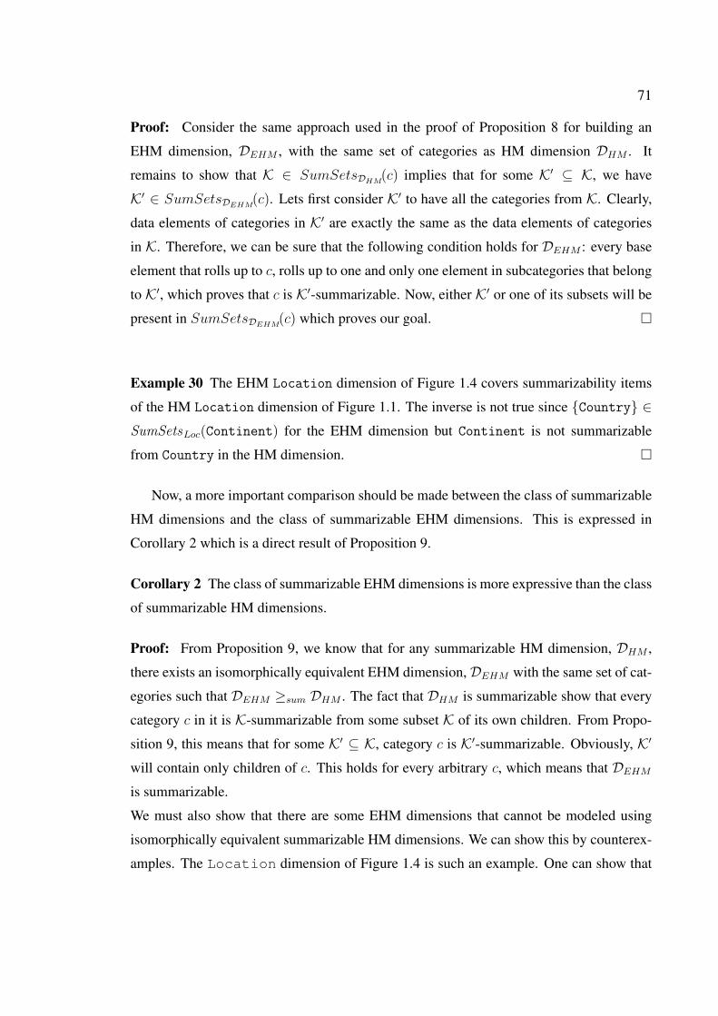
71
Proof: Consider the same approach used in the proof of Proposition 8 for building an
EHM dimension, DEHM , with the same set of categories as HM dimension DHM . It
remains to show that K ∈ SumSetsDHM(c) implies that for some K′ ⊆ K, we have
K′ ∈ SumSetsDEHM(c). Lets first consider K′ to have all the categories from K. Clearly,
data elements of categories in K′ are exactly the same as the data elements of categories
in K. Therefore, we can be sure that the following condition holds for DEHM : every base
element that rolls up to c, rolls up to one and only one element in subcategories that belong
to K′, which proves that c is K′-summarizable. Now, either K′ or one of its subsets will be
present in SumSetsDEHM(c) which proves our goal. �
Example 30 The EHM Location dimension of Figure 1.4 covers summarizability items
of the HM Location dimension of Figure 1.1. The inverse is not true since {Country} ∈SumSetsLoc(Continent) for the EHM dimension but Continent is not summarizable
from Country in the HM dimension. �
Now, a more important comparison should be made between the class of summarizable
HM dimensions and the class of summarizable EHM dimensions. This is expressed in
Corollary 2 which is a direct result of Proposition 9.
Corollary 2 The class of summarizable EHM dimensions is more expressive than the class
of summarizable HM dimensions.
Proof: From Proposition 9, we know that for any summarizable HM dimension, DHM ,
there exists an isomorphically equivalent EHM dimension,DEHM with the same set of cat-
egories such that DEHM ≥sum DHM . The fact that DHM is summarizable show that every
category c in it is K-summarizable from some subset K of its own children. From Propo-
sition 9, this means that for some K′ ⊆ K, category c is K′-summarizable. Obviously, K′
will contain only children of c. This holds for every arbitrary c, which means that DEHM
is summarizable.
We must also show that there are some EHM dimensions that cannot be modeled using
isomorphically equivalent summarizable HM dimensions. We can show this by counterex-
amples. The Location dimension of Figure 1.4 is such an example. One can show that

72
for no HM dimension with the same instance and a base category (that contains all the data
elements that have no children) the HM Location dimension becomes summarizable. �

Chapter 6
Query Answering
6.1 The Datalog Setting
With multiple dimensions, effective use of pre-computed cube views becomes a key task for
improving query answering performance. As we will show in this section, the subcategory
structure of the EHM model allows us to rewrite queries in terms of a preferred subset of
cube views and find the answer in a more efficient manner.
We will use Datalog with aggregation (see Section 2.2.3) to represent MD aggregate
queries. Datalog is a formal language with clear semantics and at the same time it is simple
and more readable than other languages such as relational algebra, SQL and MDX. For
any MD database schema, our datalog representation will include the following sets of
predicates:
• Category predicates of the form C(e) (one predicate per category identifying ele-
ments of that category),
• Subcategory predicates of the form S(e) (one predicate per subcategory identifying
elements of that subcategory),
• Parent-child predicates of the form <(e1, e2) (one predicate per dimension indicating
links in the dimension instance) and predicates the transitive closure <⋆ (e1, e2) (also
one predicate per dimension),
• Fact predicates of the form F (b1, ..., bn, z) (one predicate per fact table) where b1, ..., bnare base elements and z is a measure attribute. Without loss of generality, we will
assume that each fact table contains only one measure attribute,
• For any pair of categories c1 and c2, we will define a roll-up predicate asRc2c1(e1, e2)←
C1(e1), C2(e2), <⋆ (e1, e2),
73

74
• We will also consider a set of built-in predicates such as =, < (not to be confused
with the binary parent-child predicate), etc.
Moreover, cube views (and queries) are represented by intensional predicate symbols de-
fined using rules of datalog with aggregation. We will refer to these intentional predicates
as view predicates.
6.2 MD Aggregate Queries
Intuitively, the query answering problem can be described as follows: Given an MD ag-
gregate query q = Ψf [c1, ..., cn] where cis are categories from different dimensions, and set
of pre-computed cube views V = {v1, ..., vm}, find another query q′ that uses one or more
cube views in V and is equivalent to q (i.e. q and q′ produce the same answer for any given
database).
In a general setting, views are used to answer conjunctive queries [54]. In the case of
MDDBs, we can restrict our focus to MD aggregate queries of the form specified next.
Definition 16 Let ⟨DS,F ⟩ be an MD database schema where DS = {S1, ...,Sn} is a set
of EHM dimension schemas and F is a fact table schema. An MD aggregate query over
categories {c1, ..., cn} is a rule of the form
Q(e, Agg(z))← F (eb1 , ..., ebn , z),Rc1b1(eb1 , e1), ...,Rcn
bn(ebn , en), D(eD) (6.1)
where e, eD ⊆ {e1, ..., en}, and for any 1 ≤ i ≤ n, bi is the base category of dimension
schema Si. Also, D(eD) is a conjunction of literals non of which is a fact predicate or view
predicate. We make the additional assumption that D(eD) is not a contradiction (in which
case the query would become trivial). �
Example 31 Consider the Location and Date EHM dimensions depicted by Figure 6.1,
the fact table of Figure 1.1c. An MD aggregate query to obtain sale values in different
continents for years after 2005 can be represented as follows:
Q(cnt, year, Sum(sales)) ← F (cty, day, sales),RContinentCity (cty, cnt),
RYearDay (day, year), year > 2005
�

75
Figure 6.1: The Location and Date EHM dimensions
As stated earlier, we are looking for rewritings that are equivalent to a given aggregate
query, but instead of computing results from scratch (i.e. by aggregating over the fact table
instance), a rewriting computes results using pre-computed cube views.
Definition 17 Let V = {v1, ..., vm} be a set of pre-computed cube views and Q be an MD
aggregate query over categories {c1, ..., cn} as in Equation (6.1). Query Q′V is a rewriting
for Q over V if:
• Q and Q′V are equivalent (i.e. produce the same answer for any given database),
• Q′V is obtained through a set of rules of the following form:
P (e1, Agg(z)) ← V1(e′1, z), D1(eD1) (6.2)...
P (em, Agg(z)) ← Vm(e′m, z), Dm(eDm) (6.3)
Q′V (e, Agg(z)) ← P (e, z), D(eD) (6.4)
where for any 1 ≤ r ≤ m, Vr is a view predicate corresponding to view vr ∈ V ,
and Dr(eDr) is a conjunction of literals all of whose variables are among those in
er ∪ e′r and Dr does not contain any view predicate or fact predicate. We will refer
to rules that define predicate P (all rules above except the last one) as the core of the
rewriting. We will make the assumption that none of the rules in the core is redundant
(i.e. such that removing it would produce an equivalent query for all instances).
�

76
Notice that a rewriting as defined above, is a disjunction of aggregate queries (or a single
aggregate query if it uses only one view).
Example 32 (example 31 continued) Consider again the Location and Date EHM di-
mensions, the fact table of Figure 1.1c, query Q from Example 31 and the following set of
pre-computed cube views:
V = {v1 = Ψsum(State, Month), v2 = Ψsum(Province, Year),
v3 = Ψsum(City, Month), v4 = Ψsum(Country, Day)}.
Query Q′1 below defines a rewriting for query Q over V ′
1 = {v1, v2, v3}:
P (cnt, year, Sum(sales)) ← V1(stt,mnt, sales),RContinentState (stt, cnt),
RYearMonth(mnt, year)
P (cnt, year, Sum(sales)) ← V2(prv, year, sales),RContinentProvince (prv, cnt)
P (cnt, year, Sum(sales)) ← V3(cty,mnt, sales),RContinentCity (cty, cnt),
RYearMonth(mnt, year), City3(cty)
Q′1(cnt, year, Sum(sales)) ← P (cnt, year, sales), year > 2005
Notice in the third rule above, the use of subcategory predicate City3 to specialize view
v3 and avoid double counting of elements from subcategories City1 and City2 that have
a state or province (and therefore are already accounted for in the first two rules). We can
define another rewriting Q′2 for Q over V ′
2 = {v4} as follows:
Q′2(cnt, year, Sum(sales)) ← V4(ctr, day, sales),RContinent
Country (ctr, cnt),
RYearDay (day, year), Country1(ctr)
�
In general, the predicate in the head of the rules defining a query (or a rewriting) may select
only a subset of variables included in the view predicate (or the fact predicate) in the body.
However, in the rest of this thesis, without loss of generality we will assume that the arity
of predicates in the head is the same as the arity of view predicates (or fact predicates) in
the body. For example, instead of posing a query that asks for sales for different continents
(which omits the attribute referring to the date dimension), we can ask for sales for different
continents and category All of the date dimension.

77
6.3 The Query Answering Problem
Given an MD database schema S and a set of cube views V , we focus on the computational
problem of finding a rewriting for an MD aggregate query Q:
MDQA(Q) := {(S, V,Q′V ) | for any instance I of S , and
tuple t : I |= Q[t]⇔ I |= Q′V [t]} (6.5)
Here, the query is a fixed parameter of the problem, and the variable inputs of the compu-
tational problem are the MD database schema S (with d dimension schemas and at most k
categories and subcategories overall) and set V of m cube views. The output of the problem
is a rewriting Q′V for Q over V .
As demonstrated by Example 32, we might have multiple options (in the form of rewrit-
ings) to answer a given query. Clearly, we would like to find rewritings that are cheaper to
evaluate. The cost of evaluation depends on many factors that differ from one application
to another [54].
In this thesis, we consider rewritings that reduce the number of relation tuples involved
in the evaluation of the rewritten query. Deriving the final result of a query involves join
operations between cube views and respective roll-up relations (see Definition 17). To
lower the cost of this derivation, we would like to choose a rewriting that is connected to
cube views with fewer tuples (therefore reducing the cost of join to derive the query result).
In theory, the number of cube views reused within a rewriting can be as big as the
total number of available views. However, with a large number of re-used views in a
single rewriting, the query length becomes unreasonably large. Hence, it is natural to set
a constant limit on the number of reused views in a rewriting. In the following definition,
this limit is captured by constant C.
Definition 18 Let V be a set of pre-computed cube views and Q be an MD aggregate query.
A preferred rewriting of core size C is a rewriting of Q over V ′ ⊆ V such that |V ′| ≤ C
and for any rewriting Q′′ of Q over V ′′ ⊆ V with |V ′′| ≤ C:∑v∈V ′
size(v) ≤∑v∈V ′′
size(v)
where size(v) represents the number of tuples in cube view v. �

78
Example 33 (example 32 continued) Lets assume I is an MD database instance containing
sales values for 2000 cities spread across 50 states, 10 provinces and 20 countries over a
period of 2 years. We can compare rewritings Q′1 and Q′
2 from Example 32 as follows:∑v∈V ′
1
size(v) = size(v1) + size(v2) + size(v3)
= (50× 24) + (10× 2) + (2000× 24) = 49220∑v∈V ′
2
size(v) = size(v4) = 20× 2× 365 = 14600
Therefore, Q′2 is preferred over Q′
1. �
6.4 Query answering in EHM
We will show that with EHM dimensions (unlike HM dimensions), we can find rewrit-
ings for a query by only processing the dimension schema (as opposed to the dimension
instance). The subcategory structure of a set of compliant EHM dimensions provides an
important feature which is to specialize a cube view vi to selected subcategories chosen
from categories of vi. As an example, considering a cube view that contains sales values
of countries in different months for the EHM dimensions of Figure 6.1, we can specialize
this cube view to subcategory Country1. This way, tuples that involve element UK will
disappear from the result.
Definition 19 Let Q be an MD aggregate query (see Definition 16) over categories {c′1, ..., c′n}and v = Ψf [c1, ..., cn] be a cube view.
(a) A sub-granularity g of cube view v is a total mapping that assigns a category ci (with
1 ≤ i ≤ n) to itself or one of its subcategories (i.e. g(ci) = x implies that either x = ci or
x is a subcategory with θ(x) = ci).
(b) The specialization of cube view v to sub-granularity g for query Q, denoted vQ(g), is
defined as:
P (e′1, ..., e′n, f(z)) ← V (e1, ..., en, z),Rc′1
c1(e1, e
′1), ...,Rc′n
cn(en, e′n), S(eS) (6.6)
where S(eS) is a conjunction of subcategory predicates. The conjunction includes Si(ei)
iff (ci, si) ∈ g. �

79
Notice that, Equation (6.6) is basically a roll up from categories of view v to categories of
query Q with the exception that S(eS) filters only those elements that are part of subcate-
gories of granularity g.
Example 34 (example 31 continued) Consider the Location and Date EHM dimensions
depicted by Figure 6.1, the fact table of Figure 1.1c and a pre-computed cube view v =
Ψsum[Country, Month] containing tuples
{(Canada, Jan, 16000), (England, Jan, 11400), (US, Jan, 3000), (UK,Jan, 11400)}
In this setting:
(a) g1 = {Country → Country1, Month → Month} is a sub-granularity of v (category
Country is assigned to subcategory Country1 and category Month is assigned to itself).
g2 = {Country→ Country, Month→ Month} is another sub-granularity of v where each
category is assigned to itself (there is no filtering).
(b) The specialization of v to g1 for query Q (from Example 31) is defined by the following
rule:
P (cnt, year, Sum(sales)) ← V (ctr,mnt, sales),RContinentCountry (ctr, cnt), ...,
RYearMonth(mnt, year), Country1(ctr)
Here, subcategory predicate Country1 filters and selects tuples of view predicate V that
belong to subcategory Country1. �
Definition 20 Let ⟨DS,F ⟩ be an MD database schema where DS = {S1, ...,Sn} and each
Sk is an EHM dimension schema with mk base subcategories, namely bk1, ..., bkmk
. Also, let
v = Ψf [c1, ..., cn] be a cube view and g be a sub-granularity of v.
The base containment tensor of sub-granularity g, denoted bct(g), is an n-th rank tensor
T = (ti1...in)m1×...×mn with 1 ≤ ik ≤ mk such that:
ti1...in =n∏
j=1
f(bjij , g(cj)) (6.7)
where f(b, x) assigns a 1 or 0 to base subcategory b and subcategory x depending on
whether x is reachable from b. If x is a category (as opposed to a subcategory), then
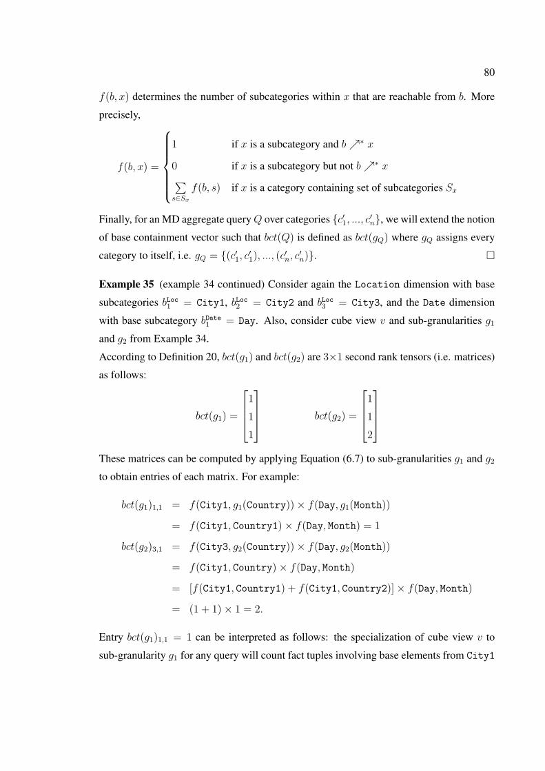
80
f(b, x) determines the number of subcategories within x that are reachable from b. More
precisely,
f(b, x) =
1 if x is a subcategory and b↗∗ x
0 if x is a subcategory but not b↗∗ x∑s∈Sx
f(b, s) if x is a category containing set of subcategories Sx
Finally, for an MD aggregate query Q over categories {c′1, ..., c′n}, we will extend the notion
of base containment vector such that bct(Q) is defined as bct(gQ) where gQ assigns every
category to itself, i.e. gQ = {(c′1, c′1), ..., (c′n, c′n)}. �
Example 35 (example 34 continued) Consider again the Location dimension with base
subcategories bLoc1 = City1, bLoc2 = City2 and bLoc3 = City3, and the Date dimension
with base subcategory bDate1 = Day. Also, consider cube view v and sub-granularities g1
and g2 from Example 34.
According to Definition 20, bct(g1) and bct(g2) are 3×1 second rank tensors (i.e. matrices)
as follows:
bct(g1) =
1
1
1
bct(g2) =
1
1
2
These matrices can be computed by applying Equation (6.7) to sub-granularities g1 and g2
to obtain entries of each matrix. For example:
bct(g1)1,1 = f(City1, g1(Country))× f(Day, g1(Month))
= f(City1, Country1)× f(Day, Month) = 1
bct(g2)3,1 = f(City3, g2(Country))× f(Day, g2(Month))
= f(City1, Country)× f(Day, Month)
= [f(City1, Country1) + f(City1, Country2)]× f(Day, Month)
= (1 + 1)× 1 = 2.
Entry bct(g1)1,1 = 1 can be interpreted as follows: the specialization of cube view v to
sub-granularity g1 for any query will count fact tuples involving base elements from City1

81
and Day only once.
On the other hand, entry bct(g2)3,1 = 2 is interpreted as follows: the specialization of
cube view v to sub-granularity g2 for any query will count fact tuples involving base ele-
ments from City3 and Day twice. This is because there are two different paths from base
subcategory City3 to category Country. �
Proposition 10 Let Q be an MD aggregate query over categories {c1, ..., cn} and V =
{v1, ..., vm} be a set of pre-computed cube views. There exists a rewriting Q′V for Q over
V , iff there exists a set {g1, ..., gm} where every gk is a sub-granularity of vk such that:
1. c1, ..., cn are all reachable from respective subcategories/categories in the range of gkfor any 1 ≤ k ≤ m, and
2. for every coordinate i1...in, (a) 0 ≤ bct(gk)i1...in ≤ 1 and (b) if bct(Q)i1...in > 0 then
bct(gk)i1...in = 1.
Furthermore, if the two conditions above are satisfied, then the set {vQ1 (g1), ..., vQm(gm)} of
specializations will be the core of a rewriting for Q.
Proof: Lets assume query Q is defined as follows:
Q(e1, ..., en, Agg(z))← F (eb1 , ..., ebn , z),Rc1b1(eb1 , e1), ...,Rcn
bn(ebn , en), D(eD)
First, we will show that for any set G = {g1, ..., gn} where gi = {ci1 → si1, ..., cin → sin}is a sub-granularity of vi and G satisfies the two conditions of Proposition 10, the following
set of rules is a rewriting of Q (notice that {vQ1 (g1), ..., vQm(gm)} is the core of the rewriting):
P (e1, ..., en, Agg(z)) ← V1(e11, ..., e1n, z),Rc1c11
(e11, e1), ...,Rcnc1n
(e1n, en),
S11(e11), ..., S1n(e1n)...
P (e1, ..., en, Agg(z)) ← Vm(em1, ..., emn, z),Rc1cm1(em1, e1), ...,Rcn
cmn(emn, en),
Sm1(em1), ..., Smn(emn)
Q′V (e, Agg(z)) ← P (e, z), D(eD)

82
We have to show that any tuple (e, m) that is in the result of Q is also in the result of Q′V
and vice-versa. Lets assume (eQ, zQ) is in the result of Q before applying D(eD). This
means that there is a set of tuples FQ = {(e1F , z1F ), ..., (erF , zrF )} from the fact table such
that every erF rolls up to eQ andr∑
i=1
ziF = zQ. Now, the core of Q′V is selecting all and
only tuples VG = {(e1G, z1G), ..., (esG, zsG)} that are members of the sub-granularities in
G. Condition 2 in Proposition 10 guaranties that if (eF , zF ) ∈ FQ then e will roll up to
exactly one tuple eG from VG (i.e. with (eG, zG) ∈ VG for some zG). Therefore, all tuples
from the fact table that are aggregated to generate (eQ, zQ) will be accounted for exactly
once within VG.
Now, the roll-up predicates in the core of Q′V perform an aggregation from tuples in
VG to respective ancestors in categories of query Q. This roll-up is possible only because
of condition 1 from Proposition 10 which guaranties that there exists an upward path to
perform such an aggregation. We have shown up to now that any tuple from the fact table
that is accounted for in the result of Q before applying D(eD) will also be accounted for
exactly once in VG (which is the extension of P in the rewriting). Hence, if we aggregate
over P and apply D(eD) to the result, we will obtain a result that is equivalent to the result
of Q.
Next, we have to prove the other side of Proposition 10, i.e. that a rewriting exists
only if there is a set {g1, ..., gn} of sub-granularities that satisfies the two conditions of
Proposition 10. Lets consider the form of a rewriting as in Definition 17. The core must
define the extension of predicate P such that any tuple from the fact table that rolls up to
some tuple from the result of Q also rolls up to the extension of P . Otherwise the last rule
(the aggregation rule that defines Q′V from P ) will not yield correct results. For this to
happen, D1(eD1), ..., Dm(eDm) have to be formed as a conjunction of literals that produce
the desired extension of P (lets refer to this extension as TargetP ). More precisely, the m
rules in the core of a rewriting, generate m partial extensions for P , namely P1, ..., Pm such
that for any i, j, Pi ∩ Pj = ∅ and∪m
k=1 Pk = TargetP .
Clearly, the literals in D1(eD1), ..., Dm(eDm) have to be expressed in terms of cate-
gories/subcategories in the schema as opposed to specific elements in dimension instances,
because the rewriting must be equivalent to Q for all possible instances of the schema. This
means that, to produce each Pi from view vi we must find a selection of category/subcategory

83
predicates that in conjunction with view predicate Vi will filter and produce Pi. This is ex-
actly what is expressed by condition 1 of Proposition 10. In addition, using links in the
schema we have to be able to propagate the results up to the level of categories in query Q
which is condition 1 of Proposition 10. �
Example 36 (example 35 continued) Consider query Q from Example 31 and sub-granularities
g1 and g2 from Example 35. g1 satisfies the two conditions of Proposition 10 because:
1. Continent and Year are reachable from Country1 and Month, and
2. bct(Q) =
1
1
2
and bct(g1) =
1
1
1
, therefore part (a) and (b) of condition 2 are both
satisfied for all coordinates of the two matrices.
As a result, specialization vQ(g1) defined below is the core of a rewriting for Q:
P (cnt, year, Sum(sales)) ← V (ctr,mnt, sales),RContinentCountry (ctr, cnt),
RYearMonth(mnt, year), Country1(ctr)
However, in the case of sub-granularity g2, bct(g2)3,1 = 2, therefore part (a) of condition 2
is not satisfied for g2.
The following theorem shows that preferred rewriting can be obtained for an MD
database comprised of compliant EHM dimensions without the need to process dimension
instances (which are usually very large).
Theorem 5 Let ⟨DS,F ⟩ be an MD database schema with overall k subcategories, q be
an aggregate query, V be a set of m pre-computed cube views and C be a constant. The
computational problem of finding a preferred rewriting of core size C for Q is O(mC ×2k(C+1)).
Proof: To obtain a preferred rewriting of core size C for Q, we can simply try every
combination of sub-granularities over all possible subsets of V with size at most equal
to C, and for each one check if it satisfies conditions of Proposition 10. Then, between

84
all candidates we can compute the sum of cube view cardinalities and select the preferred
candidate.
Lets assume DS contains d dimension schemas {S1, ...,Sd} and each dimension schema
Si has ki subcategories. There are O(mC) possible subsets of V that have a size less than
C. For each view there are less than k1× ...× kd possible sub-granularities (this is because
if we have a cube view over categories c1, ..., cn, then in a sub-granularity each ci can be
assigned to either one of the subcategories of ci or to ci itself, and we know that ci has
at most ki − 1 subcategories even in the worst case where it contains all subcategories of
the schema except All). So, overall there are O(mC × (k1 × ... × kd)C) possible sub-
granularities.
Now, for each sub-granularity we need to check the two conditions of Proposition 10.
The first condition can be checked in constant time (assuming we have identified and stored
in a data structure, the lower level subcategories that categories of each view are reach-
able from). As for the second condition, for each sub-granularity we need to compute
(k1 × ... × kd) entries of the base containment tensor. With at most C sub-granularities,
the overall complexity becomes O(mC × (k1 × ... × kd)C × C × (k1 × ... × kd)) =
O(mC × 2(C+1)lg(k1×...×kd)) = O(mC × 2(C+1)(lg(k1)+...+lg(kd))) < O(mC × 2k(C+1)). �

Chapter 7
Repairs of Non-Summarizable HM Dimensions
7.1 The EHM-based Repair Process
Summarizability allows for the correct reuse of materialized aggregate views. As discussed
in Section 2.3, it is a key property for the efficiency of OLAP systems. Therefore, it is im-
portant to address the non-summarizability issue. We do this for the HM model through
the EHM models. That is, we define EHM-based repairs of HM instances that are non-
summarizable. In other words, the EHM model allows for a repair approach that trans-
forms non-summarizable HM dimensions into summarizable EHM dimensions. This is an
alternative approach to others that directly define and compute repairs for HM instances,
e.g. those in [13, 15, 19, 20].
Figure 7.1 sketches the new approach. First, for comparison, with data repairs (left),
inconsistency of an HM model is resolved by changing links in the dimension instance
without modifying the schema (see Section 2.4). With the EHM-based repairs, we first
apply, through what we call canonical mapping, schema-based changes to transform a
possibly inconsistent HM instance into a compliant EHM instance (see Section 7.2). As
depicted in Figure 7.1, multiple compliant EHM instances may be preferred candidates
of this process, one of which will be chosen by a non-deterministic algorithm. Next, if
necessary, we apply changes to links in the dimension instance to enforce summarizability,
through a process called e-repair (see Section 7.3). We can show that, all e-repairs that
cause minimal link changes, i.e. minimal e-repairs, can be found without the need to
process the dimension instance for a given compliant EHM dimension.
As we will discuss later, our process will result in more natural solutions for the non-
summarizability problem, and will incur in less computational cost than with data re-
pairs. Notice that, if we start with a non-summarizable EHM model, as opposed to a
non-summarizable HM model, we can still apply the same process (with slight modifica-
tions to the first step, and excluding it if the input is already compliant) and obtain repairs
85

86
Figure 7.1: Data vs EHM-based repairs (complexities are only in terms of instance size)
of the EHM models.
7.2 Canonical Mapping: From HM to Compliant EHM Dimensions
Starting from an inconsistent HM instance, we can find an EHM instance which is com-
pliant, has the same set of elements and links in the dimension instance and preserves
all categories in the schema (so that users can refer to those categories in their queries).
As discussed in previous sections, a compliant EHM instance has positive computational
features compared to an HM instance. Namely, we can check summarizability, compute
summarizability sets (Section 5.3) and address the query answering problem (Chapter 6)
without processing the dimension instance. In addition, as we will show in Section 7.3,
a process similar to the data repair approach can be applied to compliant EHM instances
that, compared to data repairs for HM dimensions, results in more natural solutions to the
problem and is computationally more practical.
Definition 21 Let D = ⟨M, δ, <⟩ be an (inconsistent) HM instance over source schema
S = ⟨U, C,S,↗, θ⟩. A canonical mapping (CM) forD is a mapping fromD to a compliant
EHM instance D′ = ⟨M′, δ′, <′⟩ over target schema S′ = ⟨U, C ′,S ′,↗′, θ′⟩ with the
following properties: (a) M = M′, <=<′, C = C ′. (b) For every element e ∈ M:
θ(δ(e)) = θ′(δ′(e)) (i.e. any element belongs to the same category in the source and target
schemas). �
Example 37 Figures 1.4 and 7.2 show two different canonical mappings for the Location
dimension of Figure 1.1. Notice that, links and elements in the dimension instance and

87
Figure 7.2: A non-summarizable result of a canonical mapping for the Location dimen-sion
categories in the schema remain the same, but new subcategories are introduces (in different
ways) to make the EHM instances compliant. �
Now, with multiple options for target canonical mapping results, we would like to obtain
the ones that redistribute groups of elements as little as possible. For example, the fact that
elements Vancouver and Ottawa have been placed in different subcategories in the CM
result of Figure 7.2 will usually force queries posed on the City category to require a join
to regroup these two elements. This is why in a CM, we will try to limit redistribution of
elements as much as as possible.
Definition 22 Let D = ⟨M, δ, <⟩ be an HM instance and D′ = ⟨M, δ′, <⟩ be a canonical
transformation of D. The redistribution factor of D and D′ is defined by:
Π(D,D′) = {(e1, e2) | e1, e2 ∈M, δ(e1) = δ(e2) and δ′(e1) = δ′(e2)}
�
Intuitively, the redistribution factor is a set containing pairs of elements that were grouped
together within the same subcategory in the source HM dimension, but are grouped in
different subcategories in the result of the canonical mapping.
Example 38 Let D be the inconsistent HM dimension of Figure 1.1, D1 and D2 be results
of the canonical mappings of Figures 1.4 and 7.2, respectively. The redistribution factors

88
are as follows:
Π (D,D1 ) = {(LA, Vancouver), (LA, Ottawa), (LA, London), (Ottawa, London),
(Vancouver, London), (UK, England), (UK, Canada), (UK, US)}
Π (D,D2 ) = {(LA, Vancouver), (LA, Ottawa), (LA, London), (Ottawa, London),
(Vancouver, London), (Vancouver, Ottawa), (UK, England),
(UK, Canada), (US, Canada), (US, England)}.
�
Definition 23 A preferred canonical mapping (PCM) of (inconsistent) HM instance D is
a canonical mapping from D to D′ such that Π(D,D′) is minimal among all canonical
mapping results of D. �
Example 39 The EHM instance of Figure 1.4 is a PCM of the inconsistent HM instance
of Figure 1.1. However, the one in Figure 7.2 is not preferred, because by putting elements
Vancouver and Ottawa in the same subcategory we can obtain another CM result for
which the redistribution factor is a subset of the former CM. �
Proposition 11 There always exists at least one PCM for any HM instance D. If D is
already summarizable, it will be the only PCM of itself.
Proof: Lets consider a compliant EHM instance D′ that is isomorphically equivalent with
D. From Proposition 9, we know that such a dimension exists. Obviously, D′ is the re-
sult of a canonical mapping for D because it has the same set of elements and links in
the dimension instance, and the same categories. Also, every element belongs to the same
category in both dimensions. Now, either D′ is itself a PCM for D or there exists another
CM that has smaller redistribution factor. In either case, D has a PCM. �
By definition, there might exist more than one possible PCMs for an inconsistent HM
dimension. In theory, there might be exponentially many such PCMs. In each PCM, ele-
ments of the dimension instance are grouped in a different way in subcategories (while still
minimizing the redistribution factor).

89
7.2.1 The FIND-PCM Algorithm
Algorithm 3, called the FIND-PCM algorithm, computes one of the possible PCMs for a
given HM instance. The algorithm is composed of three steps:
1. First, for each element e, we will find ancestors of e within any category. For each
element, the result will be a mapping from category to set of elements. Any set in the
resulting map that contains more than one element indicates a source of inconsistency
(because they are different ancestors within a category for one descendant element).
So, elements within the set must be put inside separate subcategories in the final
result.
2. In the next step, using the result of step one, for each element e we will split other
elements of the same category into two disjoint sets: the consistency set β(e) and
the inconsistency set ϖ(e). β(e) will contain all elements that can potentially be in
the same subcategory as e. ϖ(e) will contain elements that have at least one shared
descendant with e, therefore can never be in the same subcategory as e.
3. Next, in a top-down order, we will start creating subcategories within each category.
Category All will have only one subcategory. Moving down in the category hierar-
chy, when we reach category c, we will take an element from that category, assign it
a new subcategory se and in a greedy fashion, one by one choose e′ ∈ β(e) and add
it to se only if it rolls up to the same subcategories as e (keeping the subcategory roll
up a total function). Now that e and e′ are assigned to the same subcategory, their
inconsistency sets must be merged, so remove any e′′ ∈ ϖ(e′) from β(e) and add it
to ϖ(e). After the iteration is done and no more element remains in β(e) to add to se,
subcategory se is finalized. Choose an element from ϖ(e), create a new subcategory
and perform a similar iteration with greedy assignment of elements until no more
element remains with unassigned subcategory.
We will demonstrate these steps with an example.
Example 40 Consider the HM instance of Figure 1.1.
Step 1: Element London will have no parent in categories State and Province, set
{England, UK} of parents in category Country, set {Europe} of parents in category Continent

90
and set {all} of parents in category All. We can find parents of other elements in each
category in a similar way.
Step 2: Having the result of step 1, we can compute the consistency set and inconsistency
set for each element. For example, elements of the {Country} category have the following
consistency and inconsistency sets:
β(USA) = {Canada, England, UK}, ϖ(USA) = ∅,
β(Canada) = {USA, England, UK}, ϖ(Canada) = ∅,
β(England) = {USA, Canada}, ϖ(England) = {UK},
β(UK) = {USA, Canada}, ϖ(UK) = {England}.
Step 3: The final step starts with creating a single subcategory within category All that
contains element all. Then, in a top-down order, we will move to the next category which
is Continent. We will (non-deterministically) take an element from this category, e.g.
NA and assign it to a new subcategory, lets call it ContinentS1. Now since β(NA) con-
tains Europe we can simply add Europe to subcategory ContinentS1. No element in
Continent remains unassigned, so we can move to category Country.
Again, we will start by choosing an element, e.g. USA and creating a subcategory for it,
lets call it CountryS1. From β(USA) we can choose an element, say England, and since
it has the same roll up structure (i.e. it rolls up to the same set of subcategories) add it to
CountryS1. Then we have to unify β(USA) and β(England) causing UK to be removed
from β(USA). Only one element remains in β(USA), namely Canada, which has the same
roll up structure and will be added to CountryS1. Next, since no element remains in
β(USA), we will extract an element from ϖ(USA), which is UK, and create a new subcategory
CountryS2 for it. Now, every element of category Country has a subcategory, so we can
move to the next category.
Creating subcategories for categories State and Province will be straightforward and
will result in one subcategory for each. In case of the City category, as before we will
start by choosing an element, say LA and creating a subcategory CityS1 for it. Then, we
will choose Vancouver from β(LA). However, Vancouver cannot be added to CityS1
since it has a different roll up structure, so it will be moved to ϖ(LA) to be processed
later. A similar scenario will occur for Ottawa and London. Hence, LA will be the only

91
element of subcategory CityS1. Element Vancouver will be chosen next from ϖ(LA) and
we will create a new subcategory for it, namely CityS2. Element Ottawa can be added to
this same subcategory, however element London will again require a separate subcategory,
namely CityS3 since its roll up structure does not match the one for Vancouver either. No
category remains, which indicates the termination of this algorithm. �
It is natural to expect the number of ancestors for any element at a single higher level
category to be less than a constant upper limit. For example, we can obviously expect
each city to roll-up to no more than one continent, or any employee to work under the
supervision of no more than two or three managers. In the following proposition, constant
A represents such an upper bound.
Proposition 12 LetD be an inconsistent HM instance, k be the number of categories, n be
the number of elements in the dimension instance and A be a maximum limit on the number
of ancestors for any element within a single higher level category. The time complexity of
the FIND-PCM algorithm is O(A2kn+ n3).
Proof: The for loop surrounding lines 13-20 will be executed for every element and each
of its ancestors, therefore at most O(A× k×n) times overall (because each element has at
most A × k ancestors). The inner for loop surrounding lines 24-26 will also run once per
each ancestor, however the cost of computing the statement at line 25 is each time O(A),
because P may contain up to A elements. Therefore, overall the statement at line 25 will
cost O(A2× k×n) in time complexity. Hence, the overall cost of the for loop surrounding
lines 8-29 is O(A2 × k × n).
The for loop surrounding lines 40-47 will be executed only once for each element in the
dimension instance. The for loop itself at worst can iterate no more than n times and each
iteration can cost O(n) (for removing an element from Ec). So, the overall time complexity
of the for loop surrounding lines 30-49 is O(n3) in the worst case. �
Proposition 13 Let D be an inconsistent HM instance and D′ be a compliant EHM in-
stance. The problem of deciding whether D′ is a PCM of D is P-TIME in the size of the
dimension instance.
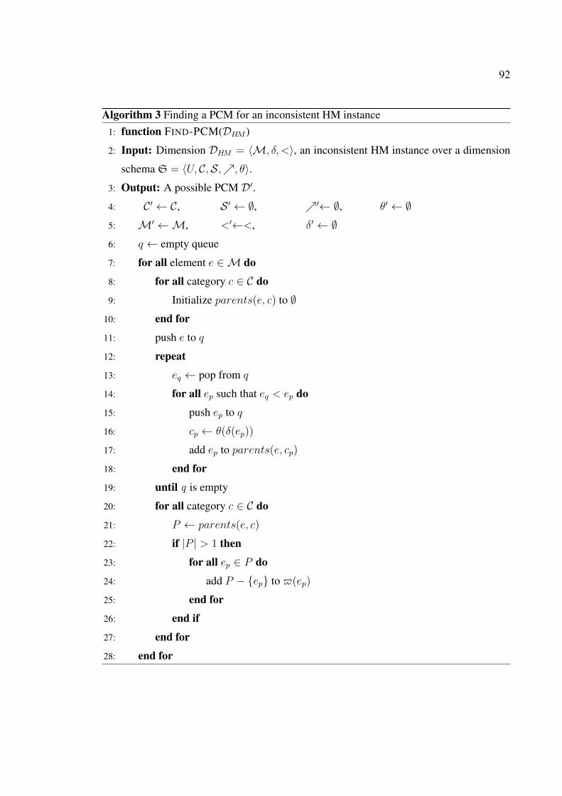
92
Algorithm 3 Finding a PCM for an inconsistent HM instance1: function FIND-PCM(DHM )
2: Input: Dimension DHM = ⟨M, δ, <⟩, an inconsistent HM instance over a dimension
schema S = ⟨U, C,S,↗, θ⟩.3: Output: A possible PCM D′.
4: C ′ ← C, S ′ ← ∅, ↗′← ∅, θ′ ← ∅5: M′ ←M, <′←<, δ′ ← ∅6: q ← empty queue
7: for all element e ∈M do
8: for all category c ∈ C do
9: Initialize parents(e, c) to ∅10: end for
11: push e to q
12: repeat
13: eq ← pop from q
14: for all ep such that eq < ep do
15: push ep to q
16: cp ← θ(δ(ep))
17: add ep to parents(e, cp)
18: end for
19: until q is empty
20: for all category c ∈ C do
21: P ← parents(e, c)
22: if |P | > 1 then
23: for all ep ∈ P do
24: add P − {ep} to ϖ(ep)
25: end for
26: end if
27: end for
28: end for
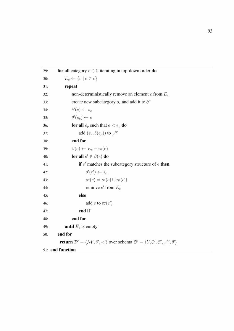
93
29: for all category c ∈ C iterating in top-down order do
30: Ec ← {e | e ∈ c}31: repeat
32: non-deterministically remove an element e from Ec
33: create new subcategory se and add it to S ′
34: δ′(e)← se
35: θ′(se)← c
36: for all ep such that e < ep do
37: add (se, δ(ep)) to↗′
38: end for
39: β(e)← Ec −ϖ(e)
40: for all e′ ∈ β(e) do
41: if e′ matches the subcategory structure of e then
42: δ′(e′)← se
43: ϖ(e) = ϖ(e) ∪ϖ(e′)
44: remove e′ from Ec
45: else
46: add e to ϖ(e′)
47: end if
48: end for
49: until Ec is empty
50: end for
return D′ = ⟨M′, δ′, <′⟩ over schema S′ = ⟨U, C ′,S ′,↗′, θ′⟩51: end function

94
Proof: First, we have to check if D and D′ have the same elements, links and categories
which can obviously be done in P-TIME. In addition, we need to check if Π(D,D′) is
minimal. If Π(D,D′) is not minimal, then there have to be at least two subcategories that
can be merged together causing Π(D,D′) to be a subset of its current value, without break-
ing the compliance condition. To check if this can happen, we can simply try all pairs of
subcategories and check if they can be merged (without violating compliance). Two sub-
categories s and s′ can be merged if they roll up to the same parent subcategories (which
can be checked in linear time wrt the schema size) and for all pairs of elements e ∈ s and
e′ ∈ s′, we have e ∈ β(e′) (meaning that combining the two elements will not cause any
non-functionality in subcategory roll ups). Using Algorithm 3, we can compute all con-
sistency sets β with P-TIME complexity in the size of the instance. Therefore, overall the
decision algorithm takes P-TIME in the size of the dimension instance. �
PCMs (and CMs) are compliant but not necessarily summarizable (although in many
cases such as the PCM of Figure 1.4 they are summarizable as well). The following propo-
sition provides a characterization of non-summarizable CMs by expressing a necessary (but
not sufficient) condition for a CM result to be non-summarizable.
Proposition 14 In any non-summarizable compliant EHM instance there exists at least one
pair of subcategories s1 and s2 such that:
1. the two subcategories have a shared parent (i.e. s1 ↗ p and s2 ↗ p for some
subcategory p),
2. they have a shared descendant base subcategory (i.e. b ↗ s1 and b ↗ s2 for some
base subcategory b), and
3. each has at least one descendant base subcategory that is not shared with the other
(i.e. there exist base subcategories b1 and b2 such that b1 ↗∗ s1 and b2 ↗∗ s2 but
neither b1 ↗∗ s2 nor b2 ↗∗ s1).
Proof: Lets consider a compliant EHM instance D. We will show that either the equal-
ity condition of Proposition 6 holds for D implying that it is summarizable or the three
conditions above altogether hold for at least one pair of subcategories.

95
For every category c of D first select all of the subcategories at the lower level as a
potential set T that satisfies the equality condition of Proposition 6. Obviously, for ev-
ery subcategory s of c, bcv(s) ≤∑
si∈Tsbcv(si). Now, if there is a subcategory s′ in c for
which the right hand side of the formula is strictly greater than the left hand side (i.e.
bcv(s′) �∑
si∈Ts′bcv(si)) this means that at least two subcategories d1, d2 ∈ Ts′ have a
shared descendant base subcategory. Now, if d1 and d2 both have other descendant base
subcategories as well, then the three conditions of the above Proposition hold for d1 and d2.
Otherwise, we can remove the one that does not have any other descendant base subcate-
gory from our initial selection of T without violating the condition bcv(s) ≤∑
si∈Tsbcv(si)
for any subcategory s of c and handle other pairs like d1 and d2 in the same way, until no
more pair remains. �
Corollary 3 Any compliant EHM instance with less than three base subcategories is sum-
marizable.
Proof: This is a direct result from Proposition 14. For the three conditions in the propo-
sition to hold, the non-summarizable EHM instance must have at least three different base
subcategories. �
To enforce summarizability, we will apply an instance-based repair approach (Section
7.3) on results of preferred canonical mappings and show that this combined approach will
produce more natural solutions with less computational cost (compared to the data repair
approach).
7.3 E-repairs
In the canonical mapping process for an inconsistent HM instance, subcategories in the
schema are adjusted so far to represent a correct model of the instance. In most cases, the
resulting compliant instance is summarizable. There are exceptional cases where the result
is still not summarizable (e.g. the canonical mapping of Figure 7.2). In the latter case, we
propose to add/remove links between subcategories, and remove links between elements

96
Figure 7.3: A minimal e-repair for the compliant EHM instance of Figure 7.2
of those subcategories accordingly, to enforce summarizability. The result is called an e-
repair. As before, dist(D,D′) denotes the symmetric difference between the sets of links
in instances of dimensions D and D′, i.e. dist(D,D′) = (<D \ <D′) ∪ (<D′ \ <D).
Definition 24 Given a compliant EHM instance D = ⟨M, δ, <⟩ over a schema S =
⟨U, C,S,↗, θ⟩: (a) an e-repair of D is a compliant EHM instance D′ = ⟨M, δ, <′⟩ over
schema S′ = ⟨U, C,S,↗′, θ⟩ such that:
1. D′ is summarizable (as characterized by Proposition 4), and
2. A new link (s, s′) in the subcategory schema of D′ can only be added if D contains
(s, s′′) for some subcategory s′′ with θ(s′) = θ(s′′) (this means that in an e-repair,
arbitrary assignment of links between subcategories from disconnected categories in
the original dimension is prohibited).
(b) a minimal e-repair of D is an e-repair D′ such that |dist(D,D′)| is minimal among all
the e-repairs of D. �
Example 41 Figure 7.3 shows a minimal e-repair for the compliant (but non-summarizable)
EHM instance of Figure 7.2 which is obtained by removing the link from London to UK in
the dimension instance and the link between corresponding subcategories. �
Proposition 15 There always exists at least one e-repair for any compliant EHM instance
D. If D is already summarizable, it will be the minimal e-repair of itself.

97
Proof: We can always construct an e-repair D′ as follows: First, for each category c we
choose a specific element ec ∈ c (it does not matter which element) and let <D′= ∅, also let
↗D′= ∅. Then, for all categories ci and cj such that ci ↗D cj and for every a ∈ ci, we add
(a, ecj) to <D′ and we add (δ(a), δ(ecj)) to↗D′ (if not previously added). The dimension
obtained is an e-repair since, by construction, satisfies the two condition of Proposition 4
for a category c and any category c′ that is a child of c by choosing T to be {δ(ec′)}. The
first condition is satisfied because dom(Rcb(D)) contains all elements in base subcategory
b and dom(RTb (D)) also contains all those elements because they all roll up to both ec and
ec′ . The second condition is satisfied and relation RT
b (D) is a function because the second
element of every tuple in that relation is ec′ . �
Example 42 The EHM instance of Figure 1.4 is already summarizable. Therefore, it is the
only minimal e-repair of itself. �
Proposition 16 There might exist exponential number of e-repairs for a compliant EHM
instance.
Proof: An e-repair can be obtained by only adding/removing links between subcategories
and links between corresponding elements (see Definition 24). To find all possible e-repairs
we can simply try all possible combinations of links between subcategories. Assuming
there are k subcategories in the schema, each link may or may not be present between any
child subcategory and a subcategory at the upper level. However, we can easily show that
for any two subcategories sc and sp, if sc ↗ sp then these subcategories can never have
a shared parent (i.e. there is no sa such that sc ↗ sa and sp ↗ sa). This means that
the hierarchy of subcategories does not have any clique of size more than two. Therefore,
according to Turan’s theorem, the number of edges between subcategories in the case were
all possible links are added (lets call this the fully connected schema) is k2
4. Therefore,
we can possibly 2k2
4 potential e-repairs (choosing possible subsets of links from the fully
connected schema). �
When a query is posed to different e-repairs (regardless of whether it is computing results
from scratch or through a pre-computed cube view at a lower level), the same query may

98
produce different results based on the chosen e-repair. This is because e-repairs add/remove
links from the dimension instance which in turn causes changes in the roll-up relations (and
hence the query results). This opens the room for the notion of consistent query answers,
i.e. answers that are shared between all minimal repairs [13]. If instead of choosing certain
answers, we focus on a specific minimal e-repair, then query answers may vary depending
on the specific repair that is chosen.
Starting from an inconsistent HM instance D, we can obtain a summarizable EHM
instance with the same categories and elements and with minimal link changes in the di-
mension instance through the following EHM-based repair process:
1. Find a preferred canonical mapping from D to D1.
2. Remove links between elements and subcategory of D1 to obtain a minimal e-repair
D2.
The first step above may produce multiple choices. The FIND-PCM algorithm only
produces one of the PCMs in polynomial time (producing all e-repairs results in higher
complexity). Also, multiple minimal e-repairs can be obtained from the PCM chosen in
the first step. However, as discussed later, all minimal e-repairs can be obtained only by
processing the dimension schema (rather than the instance which is usually very large).
Consider the initial inconsistent HM instance of Figure 1.1, and the summarizable in-
stances of Figures 1.4 and 7.3 which are results of the above process. A comparison be-
tween these results and the data repair of Figure 2.1 shows that through the data repair
process we were forced to apply much more link changes. Hence, the e-repair process
produces a more natural solution. This claim is formally expressed in the following propo-
sition:
Proposition 17 Let D be an (inconsistent) HM instance and D1 be a minimal data repair
of D. There always exists an e-repair D2 for D such that dist(D,D2) ⊆ dist(D,D1).
Proof: Consider a dimension DCM with same dimension instance as D but with one
subcategory per element and with links connecting any two subcategories that have linked
elements. DCM is clearly a CM for D because all subcategory roll ups are relations with
only one pair, and therefore they are total functions.

99
Now, data repairD1 is obtained by removing set of links Lr from instanceD and adding
set of links La to it. We can create an e-repair as follows: remove all links (e1, e2) ∈ Lr
from DCM and remove link (δ(e1), δ(e2)) from the schema of DCM . Also, add all links in
(e1, e2) ∈ La to DCM and add link (δ(e1), δ(e2)) to the schema.
We can show that in the resulting dimension, let’s call it D2, any category c is sum-
marizable from each c′ that is a child of c. This is because, we know c is summarizable
from c′ in D1. Clearly, D2 has the same elements and links in its instance as D1 (but with
more subcategories). Therefore, any base element that rolls up to c inD2, does that through
one and only one element from c′ (since we know this is the case for D1). Hence, D2 is
summarizable. �
Proposition 17 establishes a connection between data repairs and e-repairs. That is, for
every data repair of an inconsistent HM instance, there exists an e-repair obtained by apply-
ing fewer (or equal) link changes compared to link changes of the data repair. Furthermore,
we can apply the EHM-based repair process with less computational cost compared to the
cost of finding a minimal data repair. This is expressed next.
Theorem 6 Finding all e-repairs for a compliant EHM instance takes O(k2×2k(k+4)
4 ) time
where k is the size of the dimension schema (i.e. number of subcategories).
Proof: An e-repair can be obtained by only adding/removing links between subcategories
and links between corresponding elements (see Definition 24). To find all possible e-repairs
we can simply try all possible combinations of links between subcategories. Assuming
there are k subcategories in the schema, each link may or may not be present between any
child subcategory and a subcategory at the upper level. However, we can easily show that
for any two subcategories sc and sp, if sc ↗ sp then these subcategories can never have
a shared parent (i.e. there is no sa such that sc ↗ sa and sp ↗ sa). This means that
the hierarchy of subcategories does not have any clique of size more than two. Therefore,
according to Turan’s theorem, the number of edges between subcategories in the case were
all possible links are added (lets call this the fully connected schema) is k2
4. Therefore,
we have to try 2k2
4 potential e-repairs (choosing possible subsets of links from the fully
connected schema).

100
For each possible option, we have to check if it is actually an e-repair, i.e. whether it
is summarizable. According to Corollary 1, this can be done in O(k2 × 2k), leading to a
combined complexity of O(k2 × 2k × 2k2
4 ) = O(k2 × 2k(k+4)
4 ). To check if an option is
minimal, we only need to compute the total number of instance links that are associated to
the subcategory links being removed. Notice that obtaining this number only requires meta
data (in the form of a single integer) stored for each link in the schema (the total can be
obtained by summation) and does not require processing the instance (However, if we were
to generate rather than find the e-repairs, then an additional cost of iteration over instance
links would be added). Hence, the overall computational complexity is still O(k2×2k(k+4)
4 ).
�
7.4 Discussion
The purpose of the EHM-based repair process is to improve query answering performance.
To summarize the implications of each step of the process for query answering, lets as-
sume DHM is an arbitrary (i.e. not necessarily summarizable) HM dimension, DEHM is a
compliant EHM dimension obtained through canonical mapping for DHM and Derep is a
summarizable e-repair obtained for DEHM .
With an arbitrary HM dimension DHM , given an MD aggregate query Q, we can al-
ways compute correct answers to Q directly from the fact table (even if DHM is non-
summarizable). The problem is that the fact table is usually very large and such a com-
putation from scratch will be impractical and takes considerable amount of time.
The alternative approach to answering Q would be to derive the result from pre-computed
cube views that are considerably smaller than the fact table. However, there is no guaranty
that the derived result would be correct, i.e. equal to the result computed from scratch. In
addition, there is no practical way to determine beforehand, whether the results would be
equal (more precisely, the query answering problem defined in Section 6 is undecidable for
arbitrary HM dimensions).
With a compliant EHM dimension DEHM obtained through canonical mapping for
DHM , as before, any query Q can be computed from the fact table. Furthermore, Q will
yield the exact same results whether it is posed onDHM orDEHM because both dimensions

101
have the exact same elements and links in their dimension instances. Also, there is no need
for any syntactic modifications on Q since DEHM contains the exact same set of categories
as DHM in its schema. Moreover, the query answering problem is decidable for DEHM and
as long as the schema is of reasonable size, it will be practical to find a rewriting for Q over
a set of pre-computed cube views (assuming such a rewriting exists) and answer the query
with better performance.
However, DEHM may be non-summarizable in exceptional cases. So, even if we have
a complete set of pre-computed cube views over children of categories in Q, there is the
possibility that no rewriting exists for Q, in which case we would have compute the query
result from scratch.
With a summarizable dimension Derep, obtained through the EHM repair process, not
only the query answering problem is decidable, but also given a complete set of pre-
computed cube views, it is guarantied that a rewriting will exist for Q. A drawback of
Derep is that if we pose the same query Q to both DHM and Derep, we may not obtain the
exact same results (unlike DEHM that would produce the same results). This is because,
the instance of Derep has been slightly modified by adding/removing links in its dimension
instance (this same drawback will be magnified with data repairs, since they cause much
more changes in the dimension instance).

Chapter 8
Experiments
8.1 Introduction
Like most software, OLAP tools are validated through testing. However, unlike many other
software tools, testing OLAP systems needs large data sets with special characteristics.
For example, evaluating the performance of multidimensional models requires a variety of
large data sets with (summarizable or non-summarizable) dimensions that have different
graph structures and statistical properties. At the same time, due to privacy and proprietary
concerns, structurally rich data sets from real industrial applications are hard to come by
[64].
Efforts have been made to develop powerful and expressive data set generators [6, 14,
16, 34, 36, 58, 67]. However, most of these synthesizers can only generate simple tree-
shaped dimensions, but not more complicated DAG structures (as in the dimension model
of HM).
In [70], a model-based approach to synthesizing structures based on DAG for system-
atic testing and evaluation of decision support software has been proposed. The authors
present a framework that provides a small, expressive language for specifying such models.
Unfortunately, the language only supports categories as first-class elements of a schema.
As a result, it is not capable of declaring subcategories required for expressing HM models.
We have developed a Java-based framework for our experimental evaluations on HM
and EHM models. The framework allows us to create dimensions with complicated struc-
tures and instances that may contain different types of inconsistencies. The framework also
enables us to run our creation and repair algorithms and evaluate the cost of generating
EHM instances versus the benefits they provide for improving query answering perfor-
mance.
102

103
8.2 Experimental Setting
All of our experiments are executed on a system with Intel Core 2 Duo 2.10GHz proces-
sor and 4GB of RAM. The underlying implementation of the multidimensional databases
are ROLAP schemas created and instantiated using MySQL Workbench version 6.1.6 and
queried through our Java-based framework using JDBC.
To declare HM models, our framework takes as input a description of categories and
links in the schema. This input is provided in the form of simple Java entities or optionally
as XML input and contains for each category, its name plus the parent categories it is
connected to.
Furthermore, for the description of an HM instance, our framework receives the shape
(i.e. a set of statistical constraints on the distribution properties) and the size of the desired
instance. Based on the specified description, the framework creates ROLAP schemas in the
form of star tables 1 for the declared HM dimensions and populates them with records that
correspond to the specification of the dimension instance.
We have included in our framework the implementation of the FIND-PCM algorithm
(see Section 7.2.1). Provided the description of an HM dimension, the framework automat-
ically finds a preferred canonical mapping (and creates the corresponding compliant EHM
dimension). This includes creating ROLAP schemas for newly introduced subcategories
as well as the population of subcategory tables with records that indicate membership of
elements to their subcategories (as in Section 4.3).
Our experiments evaluate the cost of creating HM dimensions versus converting them
to compliant EHM dimensions. In addition, we will compare the resulting (HM and EHM)
models in terms of query answering performance using different types of queries. There
are a set of factors that can act as constant or variable settings of each experiment including:
• The number of instances: Dimension instances (and dimension tables in a ROLAP
implementation) are usually much smaller than fact tables in terms of the number of
records. But they can still vary greatly in size and range from small instances with
tens or hundreds of records, to very large instances with hundreds of thousands of
1In our implementation of star, each base element corresponds to one row of the star table, and if it hasmultiple parents in some upper level category, this is handled by a simulation of multi-valued cells usingdelimiters

104
elements. Obviously, the dimension instance size is the most important factor in the
time complexity of creation and repair algorithms as well as query answering.
• The distribution of elements within categories: Another factor that can impact the
experiment results is the relative distribution of elements within different levels (or
categories) of the schema. In the process of populating an instance, our framework
allows us to determine this factor by assigning to each category a distribution measure
relative to the base category. A distribution measure of m for category c indicates
that on average every m base elements roll up to one element from category c.
• The number of inconsistencies (and inconsistency types): The number of base
elements that cause some sort of inconsistency (in the form of heterogeneity or non-
strictness) through their upward path in the dimension instance can potentially im-
pact the costs of creating and specially repairing HM dimensions. We can define
new inconsistencies in our framework by specifying the type of inconsistency (non-
strictness or heterogeneity), the categories at which the inconsistency occurs and the
number (or rate) of base elements that encounter the inconsistency through their up-
ward path.
8.3 Creating HM Dimensions vs Finding Preferred Canonical Mappings
Our first set of experiments demonstrate the effect of dimension instance size on the time it
takes to create HM instances and the time it takes to transform them into compliant EHM
instances using the FIND-PCM algorithm. We have chosen the running example of the
Location HM dimension from Figure 1.1a for this purpose and tried multiple dimension
instance sizes.
For the first set of experiments we will keep the distribution and inconsistency rates (see
Section 8.2) constant and modify the instance size to see the effects. More specifically, we
have experimented with the creation of small to large instances ranging from 200 elements
to 200000 elements per instance. The rate of inconsistency for all the different instances of
this set of experiments is fixed at 5% including both non-strictness and heterogeneity. In
other words, at random, for every 100 base elements (cities) the data generator creates on
average 5 elements that cause either non-strictness or heterogeneity in their upward path

105
Figure 8.1: Instance size vs dimension creation time (for small instances)
through the dimension instance. In addition, the distribution of elements within categories
is fixed: for every 150 cities, we have populated the instance with 30 provinces, 50 states, 5
countries and 1 continent (as expected, regardless of instance size, there is only one element
assigned to category All).
The results are shown in Figures 8.1 (for smaller instances) and 8.2 (for larger in-
stances). The horizontal axis captures the number of instances and the vertical axis shows
time in seconds. The dashed graph represents the time it takes to create star schema for the
HM dimension schema of Location. Our framework automatically generates the follow-
ing query from the input description of the dimension schema to create the Location star
table:
CREATE TABLE T_Location (
C_City varchar(20), Primary Key (C_City),
C_Province varchar(20),
C_State varchar(20),
C_Country varchar(20),
C_Continent varchar(20),
C_All varchar(20)
);

106
Figure 8.2: Instance size vs dimension creation time (for large instances)
The solid graph in black shows the time it takes to create (populate) HM instances and the
solid gray graph depicts the time to transform the resulting instance into a compliant EHM
instance using the FIND-PCM algorithm. A simple analysis of these graphs shows that the
cost in terms of time of both creating HM instances and transforming them into compliant
EHM instances (using FIND-PCM) linearly grows as the number of instances increases.
This is regardless of whether the instance is small or very large. Also, our implementation
of the FIND-PCM algorithm for creating compliant EHM instances takes about twice as
much time as the time required for creating an HM instance.
Our next set of experiments demonstrate the effect of the schema size (number of cat-
egories) on the creation of HM instances and on running the FIND-PCM algorithm. More
specifically, we will vary the number of categories in the Location HM schema from 3
categories (City, Country and All) to 9, by adding categories one by one to lower levels
of the schema (Figure 8.3a) and then starting over and adding categories at higher levels
of the schema (Figure 8.3b). As expected, if new categories are added to lower levels (e.g.
adding a Branch category below City), the effect on the running time of FIND-PCM will
be significantly higher compared to the case where categories are added at higher levels
(e.g. adding a new category above Country). This is because an inconsistency at the level
of a category c can potentially cause the introduction of new subcategories at the level of
categories below c but not at the level of higher categories. In this set of experiments, the
instance size is fixed at 10000 elements, and as before the rate of inconsistency is fixed at
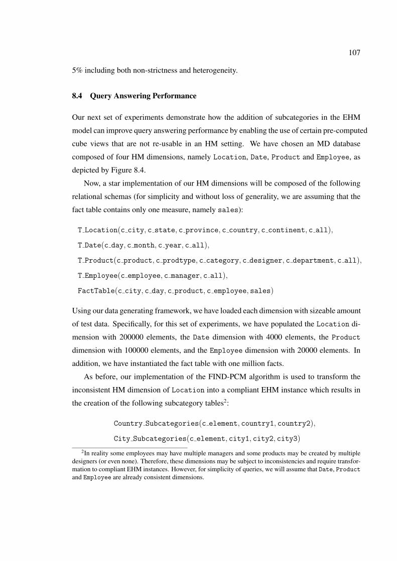
107
5% including both non-strictness and heterogeneity.
8.4 Query Answering Performance
Our next set of experiments demonstrate how the addition of subcategories in the EHM
model can improve query answering performance by enabling the use of certain pre-computed
cube views that are not re-usable in an HM setting. We have chosen an MD database
composed of four HM dimensions, namely Location, Date, Product and Employee, as
depicted by Figure 8.4.
Now, a star implementation of our HM dimensions will be composed of the following
relational schemas (for simplicity and without loss of generality, we are assuming that the
fact table contains only one measure, namely sales):
T Location(c city, c state, c province, c country, c continent, c all),
T Date(c day, c month, c year, c all),
T Product(c product, c prodtype, c category, c designer, c department, c all),
T Employee(c employee, c manager, c all),
FactTable(c city, c day, c product, c employee, sales)
Using our data generating framework, we have loaded each dimension with sizeable amount
of test data. Specifically, for this set of experiments, we have populated the Location di-
mension with 200000 elements, the Date dimension with 4000 elements, the Product
dimension with 100000 elements, and the Employee dimension with 20000 elements. In
addition, we have instantiated the fact table with one million facts.
As before, our implementation of the FIND-PCM algorithm is used to transform the
inconsistent HM dimension of Location into a compliant EHM instance which results in
the creation of the following subcategory tables2:
Country Subcategories(c element, country1, country2),
City Subcategories(c element, city1, city2, city3)
2In reality some employees may have multiple managers and some products may be created by multipledesigners (or even none). Therefore, these dimensions may be subject to inconsistencies and require transfor-mation to compliant EHM instances. However, for simplicity of queries, we will assume that Date, Productand Employee are already consistent dimensions.

108
(a) Adding categories at lower levels
(b) Adding categories at higher levels
Figure 8.3: The effect of adding categories on creation time

109
Figure 8.4: HM schemas for dimensions Location, Date, Product and Employee
Our next experiment is conducted as follows: We have materialized View cou mon emp pty =
ΨSUM [Country, Month, ProdType, Employee], a pre-computed cube view containing monthly
sales made by each employee for every product type in each country. Having this material-
ized view, we have compared the time required for answering the following set of queries
in HM and EHM (notice that in HM, because of the inconsistency of Location, category
Continent is not summarizable from category Country, therefore any query involving
Continent must be computed from scratch):
1. ΨSUM [Continent] is a one-dimensional query that computes total sales values for
different continents. In HM, this query is expressed as:
SELECT l.c_continent, sum(sales)
FROM FactTable f, T_Location l
WHERE f.c_city = l.c_city
GROUP BY l.c_continent
In the EHM setting, we can reuse the materalized view as follows:
SELECT l.c_continent, sum(sales)
FROM View_cou_mon_emp_pty v, T_Location l,
Country_Subcategories subs
WHERE v.c_country = l.c_country
AND subs.c_element = l.c_country AND subs.country1 = 1
GROUP BY l.c_continent

110
notice the addition of the subcategory table to filter elements of subcategory Country1
2. ΨSUM [Continent, Year] is a two-dimensional query that computes annual sales for
different continents. In HM, this query is expressed as:
SELECT l.c_continent, d.c_year, sum(sales)
FROM FactTable f, T_Location l, T_Date d
WHERE f.c_city = l.c_city AND f.c_day = d.c_day
GROUP BY l.c_continent, d.c_year
In the EHM setting, the query is expressed as follows:
SELECT l.c_continent, d.c_year, sum(sales)
FROM View_cou_mon_emp_pty v, T_Location l,
T_Date d, Country_Subcategories subs
WHERE v.c_country = l.c_country AND v.c_month = d.c_month
AND subs.c_element = l.c_country AND subs.country1 = 1
GROUP BY l.c_continent, d.c_year
3. ΨSUM [Continent, Year, ProductType] is a three-dimensional query that computes
annual sales values for different continents by product type. In HM, this query is
expressed as:
SELECT l.c_continent, d.c_year,
p.c_prodtype, sum(sales)
FROM FactTable f, T_Location l, T_Date d
WHERE f.c_city = l.c_city AND f.c_day = d.c_day
AND f.c_product = p.c_product
GROUP BY l.c_continent, d.c_year, p.c_prodtype
In the EHM setting, we can reuse the materalized view as follows:
SELECT l.c_continent, d.c_year,
p.c_prodtype, sum(sales)
FROM View_cou_mon_emp_pty v, T_Location l, T_Date d,
T_Product p, Country_Subcategories subs

111
WHERE v.c_country = l.c_country AND v.c_month = d.c_month
AND v.c_prodtype = p.c_prodtype
AND subs.c_element = l.c_country AND subs.country1 = 1
GROUP BY l.c_continent, d.c_year, p.c_prodtype
4. ΨSUM [Continent, Year, Employee] is another three-dimensional query that com-
putes annual sales values for different continents by each employee. In HM, this
query is expressed as:
SELECT l.c_continent, d.c_year
e.c_employee, sum(sales)
FROM FactTable f, T_Location l,
T_Date d, T_Employee e
WHERE f.c_city = l.c_city AND f.c_day = d.c_day
AND f.c_employee = e.c_employee
GROUP BY l.c_continent, d.c_year, e.c_employee
In the EHM setting, the query is expressed as follows:
SELECT l.c_continent, d.c_year
e.c_employee, sum(sales)
FROM View_cou_mon_emp_pty v, T_Location l, T_Date d,
T_Employee e, Country_Subcategories subs
WHERE v.c_country = l.c_country AND v.c_month = d.c_month
AND e.c_employee = v.c_employee
AND subs.c_element = l.c_country AND subs.country1 = 1
GROUP BY l.c_continent, d.c_year, e.c_employee
5. Similarly, ΨSUM [Year, ProductType, Employee] is expressed as:
SELECT d.c_year, p.c_prodtype,
e.c_employee, sum(sales)
FROM FactTable f, T_Date d,
T_Product p, T_Employee e
WHERE f.c_day = d.c_day AND f.c_product = p.c_product

112
AND f.c_employee = e.c_employee
GROUP BY d.c_year, p.c_prodtype, e.c_employee
And in the EHM setting it is expressed as follows:
SELECT d.c_year, p.c_prodtype,
e.c_employee, sum(sales)
FROM View_cou_mon_emp_pty v, T_Date d,
T_Product p, T_Employee e, Country_Subcategories subs
WHERE v.c_month = d.c_month
AND v.c_prodtype = p.c_prodtype
AND e.c_employee = v.c_employee
AND subs.c_element = l.c_country AND subs.country1 = 1
GROUP BY d.c_year, p.c_prodtype, e.c_employee
6. Finally, ΨSUM [Continent, Year, ProductType, Employee] computes annual sales
values made by each employee for different product types in different continents. In
HM, this query is expressed as:
SELECT l.c_continent, d.c_year, p.c_prodtype,
e.c_employee, sum(sales)
FROM FactTable f, T_Location l, T_Date d,
T_Product p, T_Employee e
WHERE f.c_city = l.c_city AND f.c_day = d.c_day
AND f.c_product = p.c_product
AND f.c_employee = e.c_employee
GROUP BY l.c_continent, d.c_year, p.c_prodtype, e.c_employee
In the EHM setting, we can reuse the materalized view as follows:
SELECT l.c_continent, d.c_year, p.c_prodtype,
e.c_employee, sum(sales)
FROM View_cou_mon_emp_pty v, T_Location l, T_Date d,
T_Product p, T_Employee e, Country_Subcategories subs
WHERE v.c_country = l.c_country AND v.c_month = d.c_month

113
Figure 8.5: Query answering time for selected queries
AND v.c_prodtype = p.c_prodtype
AND e.c_employee = v.c_employee
AND subs.c_element = l.c_country AND subs.country1 = 1
GROUP BY l.c_continent, d.c_year, p.c_prodtype, e.c_employee
Figure 8.5 shows the results of running the above queries in the aforementioned mul-
tidimensional setting. The immediate result of is that, as expected, the improvement in
query answering performance provided by the addition of subcategories in EHM (and con-
sequently the ability to reuse additional pre-computed cube views) is significant. This is
specially the case when dealing with relatively large fact tables.
A closer look at the results of Figure 8.5 also shows that the inclusion of larger dimen-
sion such as Location and Product generally has a bigger impact on query answering
compared to smaller dimensions such as Time and Employee.
Our final set of experiments demonstrate the impact of fact table size on query an-
swering time for our selected queries over HM and EHM. Specifically, we have computed
the result of ΨSUM [Continent, Year, Employee] over different fact table sizes ranging
from 20000 to 1000000 records. The result is shown in Figure 8.6. Notice that, in the

114
Figure 8.6: The impact of fact table size on query answering time
case of EHM dimensions, results have been computed through materialized cube view
View cou mon emp pty and that the view size grows in slower rate compared to the growth
rate of the fact table. Our results clearly show that with larger fact tables, the improvement
in query answering time provided by the use of EHM models is much more significant.

Chapter 9
Conclusions and Future Work
9.1 Conclusions
In this thesis, we have focused on creating MD models subject to summarizability. Pre-
vious research has mainly focused on restoring summarizability through changes made to
elements of dimension instances or the relationships/links between those elements. In-
spired by the shortcomings of previous approaches, we proposed a new MD model, as an
extension of the HM model, that is more expressive in capturing dimensions subject to
summarizability. Subcategories are the main ingredient of this extension. With the intro-
duction of subcategories, we can capture the exact structure of the dimension instance in
a much higher granularity than the granularity of the dimension instance which reduces
size of the structure. This in turn enables us to enforce summarizability conditions without
having to modify user-defined categories and with limited or no changes in the dimension
instance.
We formalized a new notion of summarizability that applies to both HM and EHM di-
mensions. Summarizable HM dimensions are still summarizable in EHM without change.
However, the inverse is not true. There exist real-world domains for which summarizable
EHM dimensions exist, however they cannot be modelled in a summarizable way using
HM.
The ADD-LINK algorithm provided in Section 4.2.1 produces EHM dimensions from
scratch by gradually adding links including endpoints. In the exceptional case where the
new link does not obey the structure of the subcategory hierarchy, new subcategories are
added accordingly.
We have provided a formal characterization of expressiveness for classes of dimension
models. We have established that the class of summarizable HM dimensions is less ex-
pressive than that of summarizable EHM dimensions. There are many commonly used
115

116
dimensions for which the HM metamodel fails to accommodate an MD model, includ-
ing instances, that satisfies summarizability. At the same time they can be modelled in a
summarizable by adding subcategories in the schema.
One of the important issues in improving query answering performance for MD databases
is to choose a set of cube views for materialization when it is too expensive to materialize
all cube views [33]. Later, when another aggregate query needs to be computed, we need
to be able to decide whether this new query can be computed using the set of materialized
pre-computed cube views. To make this latter decision, we need an efficient algorithm that
given a cube view can determine from which pre-computed cube views it can be computed.
With the HM model such an algorithm will have to process the dimension instance which is
usually very large and makes the computation impractical. With the help of the constraints
that exist in the EHM model, we have designed such an algorithm for compliant EHM
dimensions that runs in constant time with regard to the instance size.
We formally characterized the problem of query answering using views in an MD set-
ting. We express MD aggregate queries and their rewritings using the formalism of Datalog
with aggregation. We have shown that given a set of materialized pre-computed cube views
in an EHM setting, we can effectively rewrite new queries in terms of available views and
obtain query answers with better performance.
We proposed a repair approach based on the EHM model that starting from a non-
summarizable HM dimension, introduces subcategories into the schema in to produce a
compliant EHM dimension without any modification to the dimension instance or cate-
gories in the schema. Then, in exceptional case where the result is not summarizable, links
in the dimension instance are modified to enforce summarizability. In comparison with
the existing data repair approaches, our approach incurs in lower computational cost. In
addition, we have shown that the result of the EHM-based repair process is more natural
compared to existing repair approaches.
As demonstrated by our experiments, the EHM model performs well when the schema
size is relatively small. Specially in the case of computing summarizability sets and query
answering using pre-computed cube views, since the execution time of our algorithms grow
exponentially with schema size, having a very large number of categories and subcategories
will make these algorithms impractical. In these cases we may need to take advantage of

117
approximation algorithms or partial computation of outputs.
9.2 Future Work
We conclude this thesis with a list of problems for further research:
• Our COMPUTE-SUMSETS algorithm from Section 5.3 can be modified to compute
summarizability sets for a subset of categories as opposed to all of them. This will
result in lower complexity since the execution time of this algorithm grows expo-
nentially with the size of subcategories. A (manual or automated) analysis of the
history of queries imposed on the schema can direct the partial evaluation (to de-
termine which categories reused more often and select them for the computation of
summarizability sets).
• An alternative to computing summarizability sets from scratch would be to compute
them once and then check after any update, to see if the sets require modification.
Specially, in the case of HM dimensions where computing summarizability sets be-
fore queries is not efficient, this might be a viable solution that requires further in-
vestigation.
• It would be interesting to research the possible use of ontologies for designing EHM
dimensions. Semantic constraints on the subcategory category (as well as the cate-
gory hierarchy) can be checked using ontological constraints. The use of ontologies
can also aid the automation of the EHM repair process.
• Extensive research has been done in the area of cube view selection, i.e. deciding
which views to materialize [63, 5, 57, 68]. The subcategory hierarchy of a compliant
EHM dimension contains all the information required to determine a complete set of
pre-computed cube views, i.e. a set of cube views that (if materialized) is sufficient
for deriving query results at any level. There could exist multiple such sets of views.
We can combine results and methods in the literature with the additional information
provided by subcategories to better address the problem of cube view selection and
materialization.
118
• A canonical mapping in the EHM repair process may produce multiple valid op-
tions that differ in the organization of subcategories. Our FIND-PCM algorithm
non-deterministically chooses one of the options. The data warehouse users can be
involved in the decision making so that a deterministic choice can be made.
• Our relational schema extension for implementing ROLAP schemas can be formal-
ized with the notion of schema evolution [26]. This can be done by providing a
language of schema modification operators to concisely express schema changes. As
a result the DBA will be allowed to evaluate the effects of such schema changes.

Bibliography
[1] S. Abiteboul, R. Hull and V. Vianu. Foundations of Databases. Addison-Wesley, 1995.
[2] F. Afrati and R. Chirkova. Selecting and using views to compute aggregate queries.Journal Computer System Sciences, 77(6), 2011, pp. 1079-1107.
[3] R. Agrawal, A. Gupta and S. Sarawagi. Modeling Multidimensional Databases. Proc.13th International Conference on Data Engineering, 1997, pp. 232-243.
[4] M. Alviano, G. Greco and N. Leone. Dynamic Magic Sets for Programs with Mono-tone Recursive Aggregates. LPNMR 2011, pp. 148-160.
[5] K. Aouiche, P. Jouve and J. Darmont. Clustering-Based Materialized View Selectionin Data Warehouses. Advances in Databases and Information Systems 2006, pp. 81-95.
[6] A. Arasu, R. Kaushik and J. Li. Data Generation Using Declarative Constraints.SIGMOD, 2011, pp. 685-696.
[7] M. Arenas, L. Bertossi and J. Chomicki. Consistent Query Answers in InconsistentDatabases. Proc. ACM PODS’99, 1999, pp. 68-79.
[8] M. Arenas, L. Bertossi, J. Chomicki, X. He, V. Raghavan and J. Spinrad. ScalarAggregation in Inconsistent Databases. Theoretical Computer Science, 2003, 296(3),pp. 405-434.
[9] S. Ariyan and L. Bertossi. Structural Repairs of Multidimensional Databases.Proc. Alberto Mendelzon International WS of Foundations of Data Management(AMW’11), CEUR Workshop Proceedings, Vol. 749, 2011.
[10] E. Baralis, S. Paraboschi, and E. Teniente. Materialized Views Selection in a Multidi-mensional Database. Proc. 23rd International Conference on Very Large Data Bases,1997, pp. 156-165.
[11] L. Bertossi. Consistent Query Answering in Databases. ACM SIGMOD Record, June2006, 35(2):68-76.
[12] L. Bertossi. Database Repairing and Consistent Query Answering, Morgan & Clay-pool, Synthesis Lectures on Data Management, 2011.
[13] L. Bertossi, L. Bravo and M. Caniupan. Consistent Query Answering in Data Ware-houses. In Proc. Alberto Mendelzon International Workshop on Foundations of DataManagement (AMW’09), CEUR Workshop Proceedings, Vol. 450, 2009.
119

120
[14] C. Binnig, D. Kossmann, E. Lo, and M. Tamer zsu. QAGen: Generating Query-AwareTest Databases. In SIGMOD Conference, 2007, pp. 341-352.
[15] L. Bravo, M. Caniupan and C. Hurtado. Logic Programs for Repairing InconsistentDimensions in Data Warehouses. Proc. of the 4th Alberto Mendelzon InternationalWorkshop on Foundations of Data Management (AMW’10), CEUR Workshop Pro-ceedings, Vol. 619, 2010.
[16] N. Bruno and S. Chaudhuri. Flexible database generators. Proc. 31st InternationalConference on Very Large Data Bases, 2005, pp. 10971107.
[17] L. Cabibbo and R. Torlone. Querying Multidimensional Databases. Proc. DBLP’97,Springer LNCS 1369, 1997, pp. 319-335.
[18] L. Cabibbo and R. Torlone. A Logical Approach to Multidimensional Databases.Advances in Databases Technology (EDTB 1998), LNCS, volume 1337, 1998, pp.183-197.
[19] M. Caniupan. Handling Inconsistencies in Data Warehouses. In Current Trends inDatabase Technology, Springer LNCS 3268, 2004, pp. 160-176.
[20] M. Caniupan, L. Bravo, and C. Hurtado. Repairing Inconsistent Dimensions in DataWarehouses. Data & Knowledge Engineering, 2012, 79(80), pp. 17-39.
[21] M. Caniupan and A. Vaisman. Repairing Dimension Hierarchies under InconsistentReclassification. In Advances in Conceptual Modeling. Recent Developments andNew Directions, ER Workshops FP-UML, MoRE-BI, Onto-CoM, SeCoGIS, Vari-ability@ER, WISM, Brussels, Belgium, 2011, pp. 75-85.
[22] D. Cheung, B. Zhou, B. Kao, H. Lu, T. Lam and H.F. Ting. Requirement-Based DataCube Schema Design. In Proc. CIKM’99, 1999, pp. 162-169.
[23] E. Codd. Relational completeness of database sublanguage. In Database Systems(Rustin, Ed.), Prentice Hall, 1972, pp. 65-98.
[24] E. Codd, S. Codd and C. Salley. Providing OLAP (On-line Analytical Processing) touser analysis: An IT mandate. White Paper, Arbor Software, 1993.
[25] S. Cohen, W. Nutt and A. Serebrenik. Rewriting Aggregate Queries Using Views.PODS’99, 1999, pp. 155-166.
[26] C. Curino, H. J. Moon and C. Zaniolo. Graceful Database Schema Evolution: ThePrism Workbench. PVLDB, 2008, 1(1):761-772.
[27] A. Datta and H. Thomas. A Conceptual Model and Algebra for On-Line AnalyticalProcessing in Decision Support Databases. Proc. 7th Annual Workshop on Informa-tion Technologies and Systems, 1997.

121
[28] C. E. Dyreson. Information Retrieval from an Incomplete Data Cube. Proc. 22ndConference on Very Large Databases, 1996, pp. 532-543.
[29] W. Faber, G. Pfeifer and N. Leone. Semantics and complexity of recursive aggregatesin answer set programming. Artificial Intelligence, 2011, 175(1), pp. 278-298.
[30] J. Gray, S. Chaudhuri, A. Bosworth, A. Layman, D. Reichart, M. Venkatrao, F. Pel-low, and H. Pirahesh. Data Cube: A Relational Aggregation Operator GeneralizingGroup-By, Cross-Tab and Sub-Totals. Data Mining and Knowledge Discovery, 1997,1(1), pp. 29-54.
[31] M. Gyssens and L. V. S. Lakshmanan. A Foundation for Multi-DimensionalDatabases. Proc. 23rd Conference on Very Large Databases, 1997, pp. 106-115.
[32] J. Han and M. Kamber. Data Mining: Concepts and Techniques. Morgan KaufmannPublishers Inc., San Francisco, CA, 2000.
[33] V. Harinarayan, A. Rajaraman and J. Ullman. Implementing Data Cubes Efficiently.Proc. SIGMOD, 1996, pp. 205-216.
[34] J. Hoag and C. Thompson. A Parallel General-Purpose Synthetic Data Generator.SIGMOD Record, 2007, 36(1):19-24.
[35] J. Horner and I. Song. A Taxonomy of Inaccurate Summaries and Their Managementin OLAP Systems. In Conceptual Modeling - ER 2005, volume 3716 of Lecture Notesin Computer Science, 2005, pp. 433-448.
[36] K. Houkjr, K. Torp and R. Wind. Simple and Realistic Data Generation. Proc. 32ndInternational Conference on Very Large Databases, VLDB 2006, pp. 12431246.
[37] C. Hurtado. Structurally Heterogeneous OLAP Dimensions. PhD Thesis, ComputerScience Department, University of Toronto, 2002.
[38] C. Hurtado and C. Gutierrez. Computing Cube View Dependences in OLAP Dat-acubes. Proc. International Conference on Scientific and Statistical Database Man-agement, IEEE CS Press, 2003, pp. 33-42.
[39] C. Hurtado and C. Gutierrez. Equivalence of Olap Dimension Schemas. In Data Ware-houses and OLAP: Concepts, Architectures and Solutions, Wilhelminenburg Castle,Austria, 2004, pp. 176-195.
[40] C. Hurtado and C. Gutierrez. Handling Structural Heterogeneity in OLAP. In DataWarehouses and OLAP: Concepts, Architectures and Solutions, R. Wrembler and C.Koncilia (eds.), Idea Group, Inc. 2006.
[41] C. Hurtado, C. Gutierrez and A. Mendelzon. Capturing Summarizability WithIntegrity Constraints in OLAP. ACM Transactions on Database Systems, 2005,30(3):854-886.

122
[42] C. Hurtado and A. Mendelzon. Reasoning about Summarizability in HeterogeneousMultidimensional Schemas. Proc. 8th International Conference on Database Theory,2001, pp. 375-389.
[43] C. Hurtado and A. Mendelzon. OLAP Dimension Constraints. Proc. PODS’02, 2002,pp. 169-179.
[44] C. Hurtado, A. Mendelzon, and A. Vaisman. Updating OLAP Dimensions. Proc. In-ternational Workshop on Data Warehousing and OLAP (DOLAP), ACM Press, 1999,pp.60-66.
[45] C. Hurtado, A. Mendelzon and A. Vaisman. Maintaining Data Cubes under Dimen-sion Updates. Proc. ICDE’99, IEEE CS Press, 1999, pp. 346-355.
[46] W. Inmon. Building the Data Warehouse. 4th Edition, Wiley, 2005.
[47] H. V. Jagadish, L. V. S. Lakshmanan, and D. Srivastava. What Can Hierarchies Do forDataWarehouses? . Proc. 25th International Conference on Very Large Data Bases,1999, pp. 530-541.
[48] R. Kimball and M. Ross. The Data Warehouse Toolkit: the Complete Guide to Di-mensional Modeling. Wiley, 2nd edition, April 2002.
[49] L. V. S. Lakshmanan, A. Russakovsky and V. Sashikanth. What-if OLAP Queries withChanging Dimensions. Proc. ICDE’08, IEEE CS Press, 2008, pp. 1334-1336.
[50] J. Lechtenbrger and G. Vossen. Multidimensional normal forms for data warehousedesign. Information Systems, 28(5), 2003, pp. 415-434.
[51] W. Lehner. Modeling Large Scale OLAP Scenarios. Proc. 6th International Confer-ence on Extending Database Technology, 1998, pp. 153-167.
[52] W. Lehner, J. Albrecht, H. Wedekind. Normal Forms for MultidimensionalDatabases. Proc. 10th International Conference on Scientific and Statistical DatabaseManagement, 1998, pp. 63-72.
[53] H. Lenz and A. Shoshani. Summarizability in OLAP and Statistical Data Bases.Proc. International Conference on Scientific and Statistical Database Management,IEEE CS Press, 1997, pp. 132-143.
[54] A. Levy, A. Mendelzon, Y. Sagiv and D. Srivastava. Answering Queries Using Views.Proc. PODS, 1995, pp. 95-104.
[55] L. Libkin. Expressive Power of SQL. Proc. 8th International Conference on DatabaseTheory, 2001, pp. 1-21.
[56] V. Lifschitz. Circumscription. In Handbook of Logic in AI and Logic Programming,Vol. 3, Oxford University Press, 1994, pp. 298-352.

123
[57] W. Lin, I. Kuo. A Genetic Selection Algorithm for OLAP Data Cubes. Knowledge &Information Systems, 2004, 6(1), pp. 83-102.
[58] E. Lo, N. Cheng and W. Hon. Generating Databases for Query Workloads. Proc.36th International Conference on Very Large Databases, VLDB 2010, pp. 848859.
[59] E. Malinowski , E. Zimnyi. Hierarchies in a Multidimensional Model: From Con-ceptual Modeling to Logical Representation. Data & Knowledge Engineering, 2006,59(2), pp. 348-377.
[60] S. Mansmann, and M. Scholl. Empowering the OLAP Technology to Support ComplexDimension Hierarchies. International Journal of Data Warehousing and Mining, 2007,3(4), pp. 31-50.
[61] Microsoft Corporation. Multidimensional Expressions (MDX) Reference. Availableat http://msdn.microsoft.com/enus/library/ms145506.aspx, 2008.
[62] T. Niemi, M. Niinimaki, P. Thanisch, and J. Nummenmaa. Detecting summarizabilityin OLAP. Data & Knowledge Engineering, 2014, Volume 89, pp. 1-20.
[63] T. Palpanas, N. Koudas, and A. Mendelzon. On Space Constrained Set SelectionProblems. Data & Knowledge Engineering, 2008, 67(1), pp. 200-218.
[64] T. B. Pedersen, J. Gu, A. Shoshani and C. S. Jensen. Object-Extended OLAP Query-ing. Data & Knowledge Engineering, 2009, 68(5), pp. 453-480.
[65] T. B. Pedersen, C. S. Jensen, and C. E. Dyreson. Extending Practical Pre-Aggregationin On-Line Analytical Processing. Proc. VLDB’99. Morgan Kaufmann, 1999, pp.663-674.
[66] T. Pedersen, T. Jensen, and C. Dyreson. A Foundation for Capturing and QueryingComplex Multidimensional Data. Information Systems (IS), 2001, 26(5), pp. 383-423.
[67] T. Rabl, M. Frank, H.M. Sergieh and H. Kosch. A Data Generator for Cloud-ScaleBenchmarking. Proc. 2nd TPC technology conference on Performance evaluation,measurement and characterization of complex systems, 2010, pp. 41-56.
[68] A. Shukla, P. Deshpande and J. Naughton. Materialized View Selection for Multi-cubeData Models. Proc. EDBT’00, 2000, pp. 269-284.
[69] G. Spofford, S. Harinath, C. Webb, D.H. Huang, F. Civardi. MDX Solutions: WithMicrosoft SQL Server Analysis Services 2005 and Hyperion Essbase. Wiley, 2006.
[70] E. Torlak. Scalable test data generation from multidimensional models. Proc. theACM SIGSOFT 20th International Symposium on the Foundations of Software En-gineering, 2012.

124
[71] P. Vassiliadis. Modeling Multidimensional Databases, Cubes, and Cube Operations.Proc. 10th International Conference on Statistical and Scientific Database Manage-ment, 1998, pp. 53-62.
[72] M. Yaghmaie, L. Bertossi, and S. Ariyan. Repair-Oriented Relational Schemas forMultidimensional Databases. Proc. EDBT’12, 2012, pp. 408-419.