IFPRI Discussion Paper 01110

August 2011

A Multiregion General Equilibrium Analysis of Fiscal Consolidation in South Africa

Margaret Chitiga

Ismael Fofana

Ramos Mabugu

West and Central Africa Office

INTERNATIONAL FOOD POLICY RESEARCH INSTITUTE

The International Food Policy Research Institute (IFPRI) was established in 1975. IFPRI is one of 15 agricultural research centers that receive principal funding from governments, private foundations, and international and regional organizations, most of which are members of the Consultative Group on International Agricultural Research (CGIAR).

PARTNERS AND CONTRIBUTORS IFPRI gratefully acknowledges the generous unrestricted funding from Australia, Canada, China, Denmark, Finland, France, Germany, India, Ireland, Italy, Japan, the Netherlands, Norway, the Philippines, South Africa, Sweden, Switzerland, the United Kingdom, the United States, and the World Bank.

AUTHORS Margaret Chitiga, Human Sciences Research Council Executive Director, Economic Performance and Development Ismael Fofana, International Food Policy Research Institute Postdoctoral Fellow, West and Central Africa Office i.fofana@cgiar.org Ramos Mabugu, Financial and Fiscal Commission Head, Research and Recommendations Programme

Notices IFPRI Discussion Papers contain preliminary material and research results. They have been peer reviewed, but have not been subject to a formal external review via IFPRI’s Publications Review Committee. They are circulated in order to stimulate discussion and critical comment; any opinions expressed are those of the author(s) and do not necessarily reflect the policies or opinions of IFPRI.

Copyright 2011 International Food Policy Research Institute. All rights reserved. Sections of this material may be reproduced for personal and not-for-profit use without the express written permission of but with acknowledgment to IFPRI. To reproduce the material contained herein for profit or commercial use requires express written permission. To obtain permission, contact the Communications Division at ifpri-copyright@cgiar.org.

iii

Contents

Abstract v

Acknowledgements vi

1. Introduction 1

2. The Model 3

3. The Data 9

4. Simulation Scenarios 11

5. Simulation Results 13

6. Conclusion 17

Appendix: Supplementary Tables and Figure 18

References 20

iv

List of Tables

5.1—Percent change in EV of initial consumption expenses: Low scenario 14

5.2—Percent change in EV of initial consumption expenses: High scenario 14

5.3—Percent change in revenue: Low scenario 16

5.4—Percent change in revenues: High scenario 16

A.1—Dimension of the regional Social Accounting Matrix 18

A.2—Income elasticity of consumption products 18

A.3—Armington elasticities 19

List of Figures

2.1—Schematic representation of the Integrated Multi-region Applied General Equilibrium (IMAGE) model 3

2.2—Structure of interregional trade in goods and services 5

2.3—Interregional mobility of factors 6

4.1—National government spending-to-income ratio by region (%) 11

5.1—Equivalent variation of initial consumption expenses (%) 13

5.2—Variation in Theil indices (%) 13

5.3—Change in gross domestic product (%) 15

A.1—Unemployment rates by province (%) 19

v

ABSTRACT

A multiregion applied general equilibrium model is used to examine the financial interactions among spheres of government in the context of fiscal consolidation. The framework combines nine regional submodels interacting through the trading of goods and services and the mobility of labor and capital. The model integrates intergovernmental fiscal transfers, which play an important role in reducing the disparity in living standards between regions. The analysis demonstrates that the current intergovernmental revenue transfer system has significant inter- and intraregional equity effects, although its nationwide impact is less important. Reducing intergovernmental transfers leads to a reduction in welfare in the four regions where the net transfers were initially positive (Limpopo, Eastern Cape, KwaZulu-Natal, and North West Province). In contrast, welfare increases in the five other regions (Northern Cape, Mpumalanga, Free State, Gauteng, and the Western Cape). When transfer revenues fall and, consequently, regional and local government revenues drop, poor households are the most affected, as they depend more on public services that are essentially financed by governments. When the government’s fiscal position improves, it is also poor households that benefit more from additional government expenses.

Keywords: intergovernmental transfer, multiregion applied general equilibrium, consolidation, welfare

vi

ACKNOWLEDGEMENTS

We gratefully acknowledge the financial contribution of the Financial and Fiscal Commission (FFC) and thank participants in seminars held at the FFC as well as conference participants at the Economic Research Southern Africa Conference on Public Economics hosted by the University of Pretoria in 2010. Bernard Decaluwé and John Cockburn are gratefully acknowledged for development of models and data approaches used in this paper. The views expressed in this paper are those of the authors and do not necessarily represent those of the institutions that they are involved with.

1

1. INTRODUCTION

Many complex responses that arise from the interaction of the various spheres of government require appropriate techniques to effectively capture them. Applied general equilibrium (AGE) models are among the methods and tools used to better understand the interactions between national and subnational government spheres. These models are able to trace the changes in property prices, changes in opportunities for households, and migration between regions following reforms to arrangements of distributing available revenue. In addition they are able to shed light on the extent to which subnational government participates in fiscal consolidation and hence macroeconomic adjustment.

Financial interactions between spheres of government and fiscal consolidation take on an added dimension of complexity in countries with multiple government spheres. Most of the literature on the relationship between different spheres of government and their interaction on the financial side has focused on the optimal assignment of public service provision and its financing between different levels of government.1 The literature on macroeconomic management in multi-tiered governments, though less well developed, emphasizes that the increasing tendency toward decentralization and fiscal federalism raises the issue of how to maintain sustainable public finances. A key issue discussed concerns incentives faced by multi-tiered fiscal authorities, for example, the problem of soft budget constraints faced by subnational governments tasked with providing an essential service such as healthcare. This has led many countries to adopt fiscal coordination mechanisms to address the problem.2

This paper uses a multiregion AGE model to analyze the effects of government expenditures, taxation, and intergovernmental grants on equity and efficiency goals when used as an instrument of fiscal consolidation. The model is applied to South Africa, which is a unitary-state country with three spheres of government (local, provincial, and national) and a federal-like constitution. General government expenditure constitutes roughly 33 percent of gross domestic product (GDP). The portion raised nationally is approximately 29 percent, while locally raised revenue is approximately 4 percent. Provincially raised revenue is insignificant and rarely constitutes more than 2 percent of provincial revenue. The global economic crisis in 2008 and 2009 has brought to the fore a mismatch between revenues and expenditures for the country. The consequent slowdown in economic activity has reduced tax revenues. With government expenditures rising as a countermeasure to the recession as well as for capitalization of public enterprises, the government budget balance has deteriorated from a surplus of 0.9 percent of GDP in fiscal year 2008 to a projected deficit of 7.3 percent in fiscal year 2010. Gross loan debt is projected to reach 43.1 percent of GDP in fiscal year 2013, which is a significant rise from its level of 27 percent in 2009 (South Africa, National Treasury 2010). The outlook becomes even gloomier if sustainability indicators incorporate projected future events such as changes in the age structure of the population and the HIV/AIDS disease burden. Unless modified, current fiscal policy is thus likely to pass huge tax bills on to future generations.

The government has already commenced fiscal consolidation efforts, realizing that deficits of this magnitude not only lead to large public debts that may themselves become unsustainable but can destabilize the economy through rising inflation and interest rates. In this regard, the 2010/11 budget provides for a 1 percentage point reduction in the expenditure-to-GDP ratio from fiscal year 2011 to fiscal year 2013, a measure that can be viewed as a first direct signal of the government’s intent with regard to fiscal consolidation.

With fiscal consolidation a high-priority policy issue in South Africa today, it becomes important to arrive at a better understanding of how the gains and losses from deficit reduction are distributed. The cut in grants to the regions necessary to effect the 1 percentage point reduction in the expenditure-to-GDP

1 This is the classical fiscal federalism literature. Studies have looked at how different levels of government react to changes

in the balance between central government grants and local revenues, for example, the flypaper effect. See Oates (1999) for an extensive review of this literature.

2 These range from formal subnational fiscal rules (for example, expenditure and borrowing ceilings) to informal coordination mechanisms.

2

ratio can be viewed as a series of events, rather than fiscal consolidation per se, which allows us to assess the extent to which subnational governments adjust expenditures and use their own fiscal powers (where these are significant) to offset the cuts in their grant allocations.

The following section gives the structure and specificities of the multiregion AGE model used in this study. In the third section, we discuss the data requirements. The fourth section discusses the simulation and results, while the fifth section concludes the paper.

3

2. THE MODEL

This section reports the main features of the Integrated Multi-region Applied General Equilibrium (IMAGE) model built for South Africa and used to assess the equity and efficiency of the current South African intergovernmental revenue transfers (IGRT). The model combines nine submodels (Figure 2.1) that replicate the economies of the nine regions that constitute South Africa using an AGE framework.3

Figure 2.1—Schematic representation of the Integrated Multi-region Applied General Equilibrium (IMAGE) model

Rest of the world

Res

t of t

he w

orld

Res

t of t

he w

orld

Rest of the world Source: Authors. Note: AGE = applied general equilibrium; IGRT = intergovernmental revenue transfers; RSA = rest of South Africa.

An AGE model is a multimarket and multiagent system of equations that simulates the working of a market economy using real-world data. The use of AGE models in policy analysis permits the integration of both direct and indirect interactions throughout the economy; that is, if something changes in one part of the economy due to government policy, the model automatically computes the effects in the other parts.

3 Regions are synonymous with provinces in South Africa.

Linking variablesCommodity trade

Factor mobilityPrivate transfers

IGRT

Eastern CapeAGE Model

Free StateAGE Model

GautengAGE Model

KwaZulu-Natal AGE

Model

Limpopo AGE Model

Mpumalanga AGE Model

Northern CapeAGE Model

North West Province

AGE Model

CapeAGE Model

National economy

National economy

4

The neoclassical general equilibrium theory is at the core of the IMAGE model, which seeks to explain production, consumption, and prices in an economy in which producers and consumers respond to relative prices as a result of profit-maximizing and utility-maximizing behaviors, respectively. Markets simultaneously adjust relative prices in order to reconcile supply and demand decisions, and thus determine levels of production and consumption.

As noted by Partridge and Rickman (2010), although regional AGE models follow country model archetypes, they present some additional complexities, including the following:

• Regions trade not only with foreign countries, but also with other regions; therefore, the openness of the regional economy is greater than that of the country economy.

• Labor mobility is greater among regions of a country than among countries; furthermore, there is a mismatch between the place of factor employment and the place of expenditure of factor income.

• Regional saving is less likely to influence regional investment. • The intergovernmental fiscal transfers play an important role in reducing the disparity in

living standards between regions. The IMAGE model establishes the relationships among regions at four levels: (1) commodity

trade, (2) factor mobility, (3) IGRT, and (4) private transfers. These relationships are discussed separately in the following sections.

Commodity Trade Interregional trade is specified according to the information provided by the regional Social Accounting Matrixes (SAMs). Data on imported and exported commodities (and other interregional linking variables) are available in one aggregate account: the rest of South Africa (RSA). That is, the nine regional SAMs do not feature information on the region of origin and the region of destination for the traded products. The model presented here is shaped according to this information.

The first difference between the standard country model and the regional model is the number of trading partners. Specifically, the IMAGE model features three trading partners instead of the two usually encountered by standard AGE models. The availability of a given product in one region, or absorption, is met by an aggregation of products from the region, from other South African regions, and from the rest of the world. A nested constant elasticity of substitution specifies an imperfect substitution relationship among demands from the three regions. The derivative demands of the product from the region r, the RSA, and the rest of the world are closely related to the price of the product in the region, the average price of the product from the RSA, and the converted world price of the imported product.

As in standard AGE models, the region r prices of goods and services are determined through the neoclassical market-clearing price system (perfect competition hypothesis). That is, producers and consumers take as given the relative prices that equalize the quantities demanded and produced for each commodity. Therefore, simultaneously determined producer and consumer prices vary only by given tax or subsidy and margins rates.

The treatment of world prices is also similar to that in the standard AGE framework. That is, fixed international prices of imported commodities are assumed, in other words, there is no constraint on the availability or the supply of foreign goods (small country hypothesis). However, the converted prices of foreign goods, which are defined by international fixed prices, the exchange rate, and government fiscal interventions, determine the allocation of demand between national and international products.

The second feature of the IMAGE model is the interregional trade of goods and services and the treatment of export demand. In general, standard AGE models assume a fixed export demand for internationally traded commodities. However, an increasing number of models integrate a downward sloping export demand system that links export demand to the ratio of the fixed world price to the export free on board (f.o.b.) price. In the IMAGE model, the export demand addressed to a region is determined by the demand for imports from other regions of the country.

5

Interregional trade is governed by the following rule: for a given commodity, the nationwide export demand is equal to the aggregation of the nine regions’ imports (Figure 2.2). Then, the export demand addressed to a specific region follows a cost minimization rule. A constant elasticity of substitution is used to determine the export demand for the region from the nationwide export demand. Regional export prices determine the allocation of export demand among regions. Regional prices thus clear export supply and demand in the regions. Thus, the average price of imported commodities from the RSA is the average price of exported commodities by the RSA. The latter is the weighted average export price in all regions in South Africa.

Figure 2.2—Structure of interregional trade in goods and services

Impo

rt

Region 1 global demand

Region r global demand

Region 1 import ROW

Region 1 national demand

Region r national demand

Region r import ROW

Region 1 local demand

Region 1 import RSA

... Region r import RSA

Region r local demand

Imports/ exports demand South Africa

Equ

ilibr

ium

Region 1 export demand RSA

...

Region r export demand RSA

Region 1 export supply RSA

...

Region r export supply RSA

Exp

ort s

uppl

y

Region 1 local supply

Region r local supply

Region 1 export supply ROW

Region 1 national supply

Region r national supply

Region r export supply ROW

Global supply region 1

Global supply region r

Source: Authors. Note: ROW = rest of world; RSA = rest of South Africa

6

An imperfect transformation among the regional market, the RSA market, and the international market is specified for regional production. Therefore, export supplies of a product to the region, the RSA, and the rest of the world are closely linked to the price of the product in the region, the average price of the product from the RSA, and the f.o.b. price of the internationally exported product.

Adjustments in export f.o.b. prices balance export demand from and export supply to the rest of the world. Export demand from the rest of the world follows the standard specification, that is, it is downward sloping. Consequently, export demand depends on world prices and domestic f.o.b. prices.

Factor Mobility An adaption of the Harris and Todaro (1970) model of migration is used to explain the interregional mobility of factors, that is, labor and capital. The Harris and Todaro model assumes that the migration decision is based on the differentials between the expected wage in the urban sector and the wage rate in the rural sector. This implies that as long as the expected wage from migrating to the urban area is greater than the wage in the rural area, rural–urban migration occurs.

The IMAGE model considers a natural interregional flow of labor and capital explained by many factors, including the price differentials between regions. We assume that the relative changes in labor or capital flows (compared to their initial levels given by the regional SAMs) are closely linked to the changes in the ratio of national to regional prices. When the ratio is greater than 1, there is an increase in the flow of labor or capital from the region toward the rest of the country.

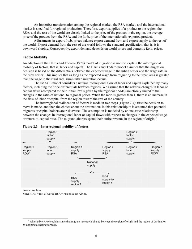
The interregional reallocation of factors is made in two steps (Figure 2.3): first the decision to move is made, and then the choice about the destination. In this relationship, it is assumed that potential migrants or capital holders are risk averse. The assumption is modeled by an inelastic relationship between the changes in interregional labor or capital flows with respect to changes in the expected wage or return-to-capital ratio. The migrant laborers spend their entire revenue in the region of origin.4

Figure 2.3—Interregional mobility of factors

Region 1 factor supply

Region r factor supply

Region 1 supply ROW

Region 1 local supply

Region 1 supply RSA

... Region r supply RSA

Region r local supply

Region r supply ROW

National

supply

RSA supply region 1

...

RSA supply to region r

Source: Authors. Note: ROW = rest of world; RSA = rest of South Africa.

4 Alternatively, we could assume that migrant revenue is shared between the region of origin and the region of destination

by defining a sharing formula.

7

Labor The change in labor supply to the RSA compared to its initial level depends on the ratio of the expected wage rate in the region and the nationwide average expected wage rate. The expected wage rates are equal to the gross wage rates adjusted by the unemployment rates. The nationwide average wage and unemployment rates are equal to the regional wage rates weighted by the regional supply and demand of labor, respectively.

The total supply of labor to the RSA is an aggregate of the regional supplies (see Figure 2.3). It is then distributed among regions according to an imperfect transformation relationship. The supply of labor from the RSA to one region is closely related to the ratio of its expected wage rates in the region and the nationwide average wage rate.

Capital The change in the supply of capital to the RSA compared to its initial level also depends on the ratio ofthe return to capital in the region and the RSA. The nationwide return to capital is an average of the regions’ returns weighted by their demand for capital.

The aggregate supply of capital is distributed among regions through a constant elasticity of transformation. The supply of capital from the RSA to the region is also related to the region’s return to capital and the nationwide average return to capital.

Intergovernmental Fiscal Transfers The IMAGE model accounts for three spheres of government: national, regional, and local. Each of these spheres of government is assigned certain powers, functions, and financial resources, each of which in turn may be exclusive, concurrent, or shared. Although the national government raises the vast majority of aggregate revenues, its expenditure responsibilities are much lower. There is thus a mismatch between revenues raised and expenditure responsibilities. A converse mismatch exists at the provincial level. This mismatch is known as vertical fiscal imbalance. Horizontal fiscal imbalance exists among regions, and also among localities within regions where different regions have different abilities to raise funds. Thus, there are massive relative differences among regions’ expenditure responsibilities and existing (as well as potential) revenue sources.

Each government sphere spends on providing public services, subsidizing the national economy (activities and products), and transferring revenues to other governments and institutions. The IGRT are modeled in a standard fashion, that is, they are assumed fixed in real terms. Government fiscal policies also follow the standard specification; the national government expenses in a given region are exogenous. While national government fiscal balance is endogenously determined in all regions, its overall balance is exogenous. Therefore, a revenue-neutral hypothesis is assumed for the national government, and its revenue loss, if any, is compensated by an endogenous uniform tax on household gross incomes across all regions. Rigidity in expenses and revenue-neutral assumptions are also assumed for regional and local governments. Compensatory taxes at endogenous uniform rates are applied to households’ gross incomes.

Interregional Private Transfers and Other Specificities The study uses a standard formulation in modeling private transfers, that is, they are fixed among regions as well as between a given region and the rest of the world. The assumptions associated with the rest of the model are discussed below.

Regional Supply and Demand Producers maximize their profit under a given technology and prices. Industry-specific producers are modeled as representative producers that are assumed to have a nested constant elasticity of substitution (CES) production technology. In addition, there is a separation between production activities and

8

commodities. A fixed proportional relationship between activity output and the domestic supply of commodities permits any activity to produce one or multiple commodities and any commodity to be produced by one or multiple activities.

Consumers’ behavior is rational, which implies that in the presence of complete markets, there is a separation between their production and consumption decisions. With the fixed factor endowments assumption, their incomes are closely related to the return to these factors. Consumers maximize their utility under limited budgets and given market prices. In addition, households are modeled as representative agents that are assumed to have Stone-Geary types of preferences.

Institutional Constraints AGE models differ primarily in the choices of closure rules that equilibrate commodity, factor, and foreign exchange markets. These models also differ in the rules specified to reconcile the government budget constraint and in the mechanism used to equilibrate savings and investment levels in the economy.

The labor market is assumed to be fully segmented. Each category of labor is assumed to be perfectly mobile across industries. Skilled workers are fully employed in the economy, although low rates of frictional unemployment5 are observed. The skilled labor market is assumed to be perfectly competitive, so that the prevailing wage rates equalize exogenous supply and endogenous demand for high-skilled workers. In contrast, there is imperfect competition in the unskilled labor markets, where the total demand does not equal the total supply. There is an excess supply of labor, which remains unemployed. The wage rate paid to unskilled workers is closely related to the unemployment rates through a wage curve specification.

Institutional units are endowed with one type of capital, which is mobile among industries with one return to capital in the economy. The analysis is performed in a static comparative, which does not imply capital accumulation and investment rules. As a consequence, we assume exogenous investment and capital supply. Therefore, saving is investment driven. Savings are generated by exogenous constant rates for households and by residual savings for firms. Savings of the national, provincial, and local governments are exogenous, as are savings of the RSA and the rest of the world.

Although every region exchanges directly with the rest of the world through the trade of goods and services and other transfers, the external current account balance is specified at the national level. The nationwide balance of the external current account is exogenous. Thus, an endogenous exchange rate or the relative price of goods and services traded with the rest of the world clears the external current account.

However, regional submodels also feature external current accounts with the RSA. To avoid free lunches among regions, the balances of the external current accounts with the RSA are fixed; they are balanced through adjustments in region-specific exchange rates. The latter, defined as the relative price of goods and services traded with the RSA, are set as numeraires.

5 Frictional unemployment exists because both jobs and workers are heterogeneous. A mismatch related to skills, payment,

working time, location, attitude, and tastes can result between the supply of and demand for labor.

9

3. THE DATA

The IMAGE model is operationalized through the calibration procedure, which consists of finding parameters that permit equations to exactly reproduce the benchmark situation given by nine region-level SAMs.6 The structure and analysis of the regional SAMs are presented next.

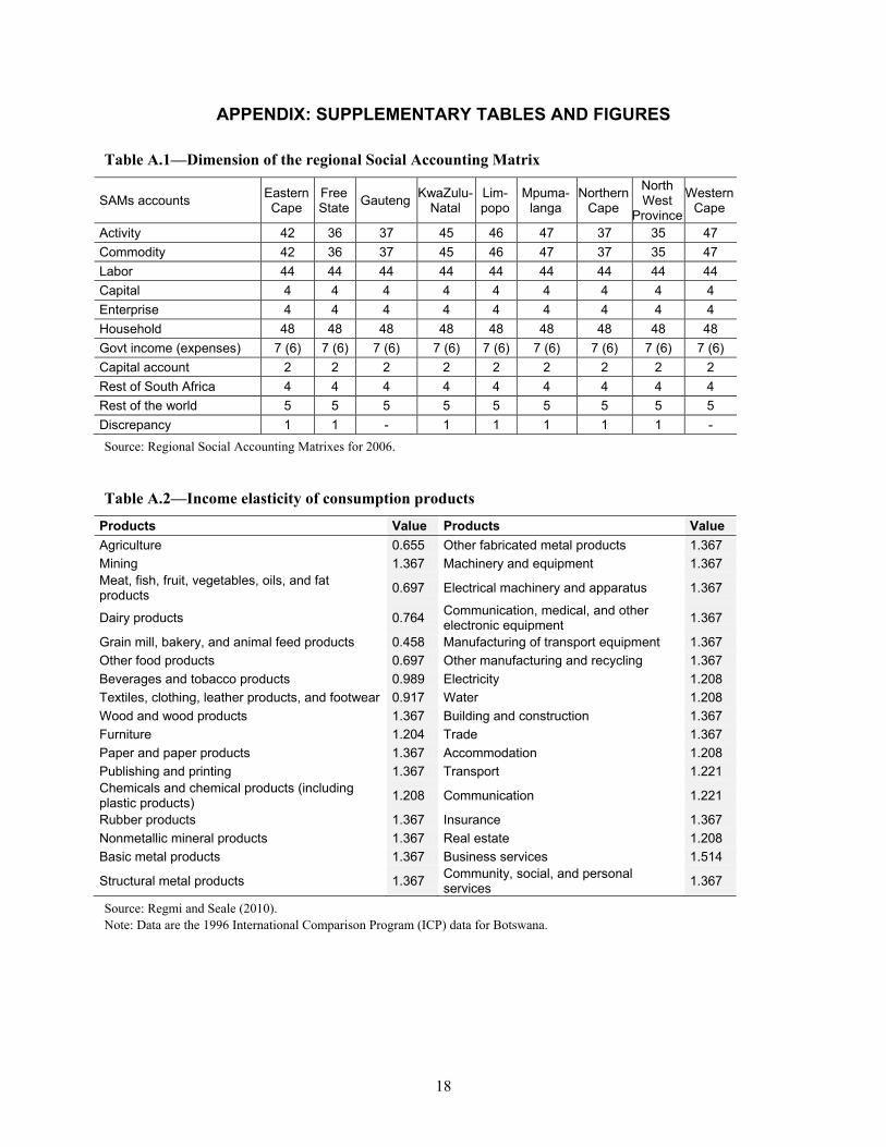
Regional Social Accounting Matrixes Regional SAMs are available for the nine regions that constitute South Africa. All SAMs are for the year 2006 and are structured to include the following (see Table A.1 in the appendix):

• 35 to 47 accounts for activities/commodities • 44 accounts for labor payments divided into 4 population groups and 11 occupations • 4 accounts for capital payments or the gross operating surplus (GOS) • 4 accounts for enterprises • 48 accounts for households, disaggregated into 4 population groups and 12 consumption deciles • 7 accounts for government income sources and 6 accounts for its expenditure items • 2 accounts for government capital accumulation and corporation and household capital

accumulation • 4 accounts for the rest of South Africa • 5 accounts for the rest of the world • 1 account for residuals and discrepancies

The adjustment procedure aims to set up a common framework for the nine regional SAMs, as well as being consistent with the standard structure of AGE models:

• Activities and products are aggregated into a suitable number of accounts according to the mapping made among the 9 regional SAMs in order to generate a uniform framework with 35 industries/commodities, detailed as follows: 1 agriculture, 1 mining, 4 food, 1 beverage, 19 manufacturing, and 9 services.

• The 44 accounts for labor payments are aggregated into the 11 occupational groups. • The 4 accounts for enterprises are grouped into 2 categories: “Public Enterprise” and “Private

Business Enterprise,” the latter including “Combi-Taxi Enterprise” and “Informal Enterprise.” • The 48 accounts for households are aggregated according to the 12 consumption deciles. • Income and expense accounts of the three levels of government—national, provincial, and

local—are adjusted to match receipts (row) and spending (column). • The 4 accounts for the rest of South Africa are aggregated into one account. • The 5 accounts for the rest of the world are also aggregated into one account. • Institutional accumulation accounts are aggregated into one account. • The allowance for depreciation or payments of capital recorded directly in the capital account is

first transferred to institutional units and then channeled to the capital account; the model follows the principle that saving is made by institutional units, either resident or nonresident.

• Residual accounts are cancelled out by combining them into the change in inventories featured in the accumulation account.

6 The SAMs are provided by the South African Department of Trade and Industry and were constructed by Coningharth

Economists in 2008.

10

Other Data Alongside the SAM data, the calibration procedure of the IMAGE model requires additional information—essentially the elasticities, the Frisch parameter, and the unemployment rates. With the exception of unemployment rates, which are different from one region to another (Figure A.1 in the appendix), the value of parameters chosen for regional submodels are identical.

The values of the income elasticity of demand are drawn from the work done by the Economic Research Service of the U.S. Department of Agriculture for 114 countries (Table A.2 in the appendix).7 The elasticity of wage rates with respect to the unemployment rate is set at -0.1, according to estimates by Kingdon and Knight (2005). The value of -3.34 is chosen for the Frisch parameter, an estimate for middle-income countries by Hertel, McDougall, and Dimaranun (1997). The elasticity of substitution between capital and labor is fixed at 2.5, the highest value surveyed by Annabi, Decaluwé and Cockburn (2006). The trade elasticities are estimated by Gibson (2003) for the Armington elasticities (Table A.3 in the appendix), and by Behar and Edwards (2004) for the export elasticities. The latter take the values of 1.3 for the transformation elasticity and 6.0 for the export demand elasticity.

The next set of parameters related to the interregional relationship is (1) the import and export elasticities, (2) the elasticity of factor mobility among regions with respect to prices, and (3) the transformation elasticity of factors among regions. As long as we do not have estimates for these parameters and the results of this analysis are likely to be influenced by their values, then the main simulation is carried out under two scenarios: low and high interregional relationships. These are discussed in depth in the following section.

7 The data are available at www.ers.usda.gov/data/internationalfooddemand. The values estimated for Botswana are used for

South Africa because this database does not cover the latter country. South Africa and Botswana are comparable countries according to the Human Development Indexes annually computed by the United Nations Development Programme (UNDP).

11

4. SIMULATION SCENARIOS

The IMAGE model developed for South Africa is used to assess the effectiveness of the current IGRT. The degree to which the national government’s equity goal is achieved through the current IGRT is quantified. Our simulation is based on the vertical imbalance of national government revenues and expenses among regions.

We first present the revenues and expenses of the national government in each region to better understand the simulation performed later. Figure 4.1 shows the disparities between collected revenues and expenses by the national government in all regions.

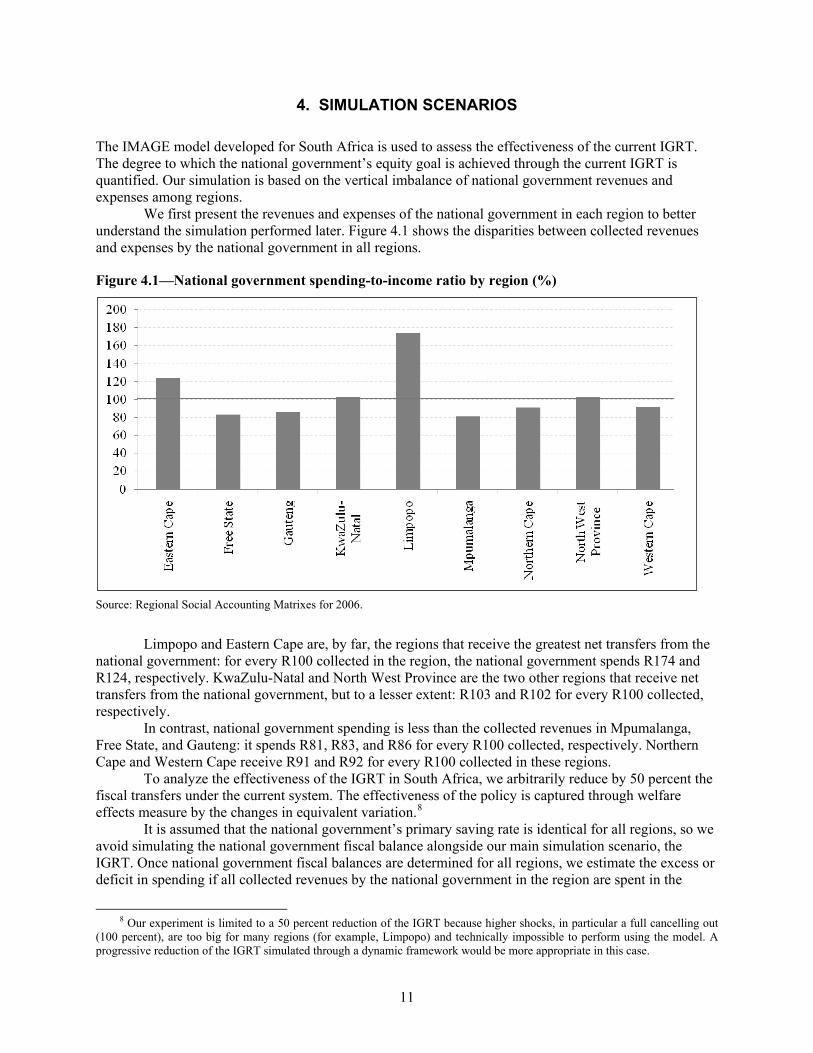
Figure 4.1—National government spending-to-income ratio by region (%)

Source: Regional Social Accounting Matrixes for 2006.

Limpopo and Eastern Cape are, by far, the regions that receive the greatest net transfers from the national government: for every R100 collected in the region, the national government spends R174 and R124, respectively. KwaZulu-Natal and North West Province are the two other regions that receive net transfers from the national government, but to a lesser extent: R103 and R102 for every R100 collected, respectively.

In contrast, national government spending is less than the collected revenues in Mpumalanga, Free State, and Gauteng: it spends R81, R83, and R86 for every R100 collected, respectively. Northern Cape and Western Cape receive R91 and R92 for every R100 collected in these regions.

To analyze the effectiveness of the IGRT in South Africa, we arbitrarily reduce by 50 percent the fiscal transfers under the current system. The effectiveness of the policy is captured through welfare effects measure by the changes in equivalent variation.8

It is assumed that the national government’s primary saving rate is identical for all regions, so we avoid simulating the national government fiscal balance alongside our main simulation scenario, the IGRT. Once national government fiscal balances are determined for all regions, we estimate the excess or deficit in spending if all collected revenues by the national government in the region are spent in the

8 Our experiment is limited to a 50 percent reduction of the IGRT because higher shocks, in particular a full cancelling out

(100 percent), are too big for many regions (for example, Limpopo) and technically impossible to perform using the model. A progressive reduction of the IGRT simulated through a dynamic framework would be more appropriate in this case.

12

region. The excess/deficit in spending is then calculated in proportion to the initial national government spending in terms of transferred revenues to the region. In the baseline scenario, this excess/deficit in spending is nil. In the simulation scenario, it is assumed that 50 percent of the excess in spending is cancelled out for some regions and 50 percent of the deficit in spending is transferred back to other regions.

Limpopo, Eastern Cape, KwaZulu-Natal, and North West Province receive less transfer revenues when 50 percent of the IGRT is cancelled out, and consequently national government spending falls in these regions. In contrast, Northern Cape, Western Cape, Free State, Mpumalanga, and Gauteng have additional fiscal spare, that is, national government spending increases in these regions.

National government fiscal policy is not affected by the changes in transfer revenues, as it is retransferring revenues among regions. However, regional government fiscal policy is directly affected by the changes in transfer revenues. We adopt a revenue-neutral hypothesis for regional governments so that with fixed regional expenses and savings, the regional government budget is balanced through a compensatory tax or subsidy on households’ gross income.

The 50 percent reductions of grants are performed under two scenarios: low and high interregional trade and factor mobility. The low interregional relationship scenario assumes that interregional trade elasticities are identical to international trade elasticities. Assuming no changes in regions’ ownership of factors and consequently temporary mobility of labor, we assume an inelastic interregional supply of labor and capital with respect to the changes in their relative regional prices. While the elasticity value of 0.1 is set for labor, a relatively more flexible value of 0.3 is chosen for capital. An identical elasticity value for labor mobility and the transformation elasticity is assumed, that is, after the decision to supply more or less labor to the other regions is made, the choice of the destination is still limited because of the hypothesis of temporary mobility of labor. However, it is assumed that the choice of the destination (the transformation elasticity) of capital is twice as flexible as the supply elasticity. As long as the openness of the regional economy is greater than that of the country economy, results drawn from the low scenario should be interpreted as lower bound results. Therefore, the high interregional relationship scenario measures the sensitivity of the results to higher economic interaction among regions. In this regard, the elasticities are set at values three times higher than their counterpart in the low scenario. The next section presents the results of the simulation under the two scenarios of interregional economic interactions.

13

5. SIMULATION RESULTS

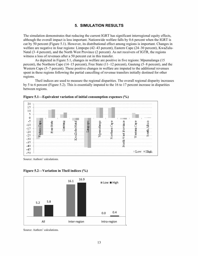
The simulation demonstrates that reducing the current IGRT has significant interregional equity effects, although the overall impact is less important. Nationwide welfare falls by 0.6 percent when the IGRT is cut by 50 percent (Figure 5.1). However, its distributional effect among regions is important. Changes in welfare are negative in four regions: Limpopo (42–43 percent), Eastern Cape (24–30 percent), KwaZulu-Natal (3–4 percent), and the North West Province (2 percent). As net receivers of IGTR, the regions witness a loss of revenues after a 50 percent cut in this transfer.

As depicted in Figure 5.1, changes in welfare are positive in five regions: Mpumalanga (15 percent), the Northern Cape (14–15 percent), Free State (11–12 percent), Gauteng (5–8 percent), and the Western Cape (5–7 percent). These positive changes in welfare are imputed to the additional revenues spent in these regions following the partial cancelling of revenue transfers initially destined for other regions.

Theil indices are used to measure the regional disparities. The overall regional disparity increases by 5 to 6 percent (Figure 5.2). This is essentially imputed to the 16 to 17 percent increase in disparities between regions.

Figure 5.1—Equivalent variation of initial consumption expenses (%)

Source: Authors’ calculations.

Figure 5.2—Variation in Theil indices (%)

. Source: Authors’ calculations.

5.2

16.1

0.0

5.8

16.9

0.4

All Inter-region Intra-region

Low High

14

Although the overall intra-regional disparities remain unchanged (Figure 5.2), the inter-regional disparities are important and vary from one region to another. Disparities between top and bottom income categories increase in Limpopo and the Eastern Cape, regions initially receiving net positive IGRT (Tables 5.1 and 5.2). The reduction in revenue transferred to other regions—consequently, an increase in national government spending in the region—benefits the bottom income groups in the Northern Cape, Mpumalanga, and Free State.

Table 5.1—Percent change in EV of initial consumption expenses: Low scenario

Source: Authors’ calculations. Note: EV = equivalent variation.

Table 5.2—Percent change in EV of initial consumption expenses: High scenario

Household category

Eastern Cape

Free State Gauteng

KwaZulu- Natal

Lim-popo

Mpuma-langa

Northern Cape

North West Province

Western Cape

P1 -22.1 10.4 8.0 -2.7 -40.8 15.0 13.2 -1.9 5.0 P2 -20.3 10.4 7.0 -2.9 -37.9 12.4 11.4 -2.2 4.4 P3 -20.8 10.5 6.8 -2.9 -38.4 12.4 11.3 -2.0 4.6 P4 -20.7 10.5 6.6 -2.9 -38.8 12.7 10.2 -2.0 4.7 P5 -20.9 10.5 6.8 -3.0 -38.3 12.7 9.8 -2.1 4.6 P6 -21.4 10.7 6.7 -3.0 -39.3 13.1 9.2 -2.0 4.6 P7 -22.3 10.7 6.9 -3.0 -40.6 12.6 9.5 -2.2 4.6 P8 -22.8 10.8 6.8 -3.1 -41.0 13.1 15.8 -2.1 4.7 P9 -23.0 11.0 6.7 -3.0 -42.6 13.8 15.1 -2.0 4.9 P10 -28.9 12.3 7.6 -3.3 -52.1 17.5 13.2 -1.9 5.1 P11 -33.7 13.1 9.3 -3.3 -50.1 17.4 17.7 -2.3 5.3 P12 -25.0 14.4 8.1 -3.1 -43.0 15.0 58.7 -2.0 5.5 ALL -24.2 11.9 7.6 -3.1 -42.6 14.5 15.1 -2.1 5.2 Source: Authors’ calculations. Note: EV = equivalent variation.

Therefore, halving the IGRT in South Africa would lead to an increase of regional disparities. Regions such as Limpopo and Eastern Cape witness significant welfare losses compared to other regions. In the same vein, low-income households are heavily hit compared to the middle- and high-income households within these regions. Regions that were initially transferring revenue witness welfare gains, and their income disparities fall when the IGRT is reduced by 50 percent.

Household category

Eastern Cape

Free State

Gauteng KwaZulu-Natal

Lim-popo

Mpuma-langa

Northern Cape

North West Province

Western Cape

P1 -27.2 9.8 5.9 -3.4 -39.8 14.4 10.8 -2.3 6.3 P2 -26.0 9.8 5.6 -3.8 -36.6 12.5 8.7 -2.5 6.0 P3 -26.6 9.9 5.2 -3.7 -37.3 12.9 8.4 -2.2 6.3 P4 -26.3 9.9 4.8 -3.6 -37.8 13.1 9.3 -2.2 6.6 P5 -26.5 9.8 5.1 -3.7 -36.8 12.9 9.0 -2.3 6.4 P6 -26.7 10.0 4.8 -3.6 -38.2 13.4 9.9 -2.2 6.3 P7 -27.8 10.0 5.3 -3.4 -39.4 12.7 10.9 -2.3 6.2 P8 -27.9 10.1 4.8 -3.5 -40.0 13.1 16.2 -2.3 6.5 P9 -28.1 10.4 4.4 -3.4 -41.6 14.2 15.1 -1.9 6.9 P10 -35.4 11.6 4.5 -3.7 -51.7 17.9 13.8 -1.8 7.0 P11 -41.9 12.4 6.9 -3.9 -49.8 17.3 18.5 -2.5 7.2 P12 -31.5 13.9 5.2 -3.7 -42.2 15.4 54.8 -1.9 7.4 ALL -30.4 11.3 5.1 -3.7 -41.7 14.8 14.3 -2.1 7.0

15

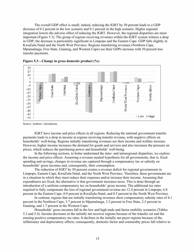
The overall GDP effect is small; indeed, reducing the IGRT by 50 percent leads to a GDP decrease of 0.2 percent in the low scenario and 0.1 percent in the high scenario. Higher regional integration lowers the adverse effect of reducing the IGRT. However, the regional disparities are more important (Figure 5.3). The group of regions receiving revenues within the IGRT system witness a drop in GDP; the decrease is particularly significant in Limpopo and the Eastern Cape. GDP falls slightly in KwaZulu-Natal and the North West Province. Regions transferring revenues (Northern Cape, Mpumalanga, Free State, Gauteng, and Western Cape) see their GDPs increase with 50 percent less transfer payments.

Figure 5.3—Change in gross domestic product (%)

Source: Authors’ calculations.

IGRT have income and price effects in all regions. Reducing the national government transfer payments leads to a drop in income in regions receiving transfer revenue, with negative effects on households’ well-being. Regions initially transferring revenues see their income and welfare increase. However, higher income increases the demand for goods and services and also increases the pressure on prices, which reduces the purchasing power and households’ well-being.

In the following sections, to better understand the inter- and intraregional disparities, we explore the income and price effects. Assuming a revenue-neutral hypothesis for all governments, that is, fixed spending and savings, changes in revenue are captured through a compensatory tax or subsidy on households’ gross incomes and, consequently, their consumption.

The reduction of IGRT by 50 percent creates a revenue deficit for regional governments in Limpopo, Eastern Cape, KwaZulu-Natal, and the North West Province. Therefore, these governments are in a situation in which they must reduce their expenses and/or increase their income. Assuming that expenditures are fixed, the alternative is that government increases taxes. This is done through an introduction of a uniform compensatory tax on households’ gross income. The additional tax rates required to fully compensate the loss of regional government revenue are 12.4 percent in Limpopo, 6.8 percent in the Eastern Cape, 0.9 percent in KwaZulu-Natal, and 0.5 percent in the North West Province.

In contrast, regions that are initially transferring revenues show compensatory subsidy rates of 4.1 percent in the Northern Cape, 3.7 percent in Mpumalanga, 3.2 percent in Free State, 2.5 percent in Gauteng, and 1.7 percent in the Western Cape.

Households’ gross incomes fall in the low and high trade and factor mobility scenarios (Tables 5.3 and 5.4). Income decreases in the initially net receiver regions because of the transfer cut and the ensuing positive compensatory tax rates. It declines in the initially net payer regions because of the inflationary and depreciatory effects; consequently, domestic factor and commodity prices fall relative to

16

external prices. Consumer price indexes also fall, and, consequently, real consumption increases for the net payers and decreases for the net receivers.

Because of the regressive nature of the compensatory tax, and eventually public expenses when government must cut its expenses instead of increasing taxes, poor households are hit hard in regions where its rate increases. In contrast, poor households benefit more in regions where the compensatory tax rate falls.

Table 5.3—Percent change in revenue: Low scenario

Eastern Cape

Free State Gauteng

KwaZulu- Natal

Lim-popo

Mpuma-langa

Northern Cape

North West Province

Western Cape

Gross income -4.3 -3.6 -2.9 -3.7 -3.2 -3.7 -3.1 -3.6 -3.5 Compensatory tax rate 6.8 -3.2 -2.5 0.9 12.4 -3.7 -4.1 0.5 -1.7 Disposable income -12.3 -0.2 -0.2 -4.8 -16.6 0.3 2.5 -4.4 -1.6 Consumer price index -4.5 -3.3 -1.6 -3.7 -3.9 -3.8 -1.7 -3.6 -3.5 Real consumption -8.3 4.0 1.4 -1.1 -13.2 4.4 16.0 -0.8 2.1

Source: Simulation results.

Table 5.4—Percent change in revenues: High scenario

Eastern Cape

Free State Gauteng

KwaZulu- Natal

Lim-popo

Mpuma-langa

Northern Cape

North West Province

Western Cape

Gross income -1.3 -0.8 -0.6 -1.0 -0.7 -1.3 -1.2 -1.2 -0.9 Compensatory tax rate 6.2 -3.2 -2.4 0.8 11.9 -4.0 -4.4 0.4 -1.3 Disposal income -8.6 2.8 2.1 -1.9 -13.8 3.2 5.2 -1.7 0.6 Consumer price index -1.4 -0.8 -0.2 -1.0 -1.2 -1.1 0.6 -1.0 -0.9 Real consumption -7.5 4.3 2.4 -0.9 -12.9 4.5 17.8 -0.6 1.6

Source: Authors’ calculations.

17

6. CONCLUSION

Previous studies of fiscal consolidation attempts have tended to focus solely on general government; this paper, in contrast, has established an important role for subnational government in fiscal consolidation. Using a multiregion AGE model, we have provided a picture of how efficiency and equity goals are affected. Although the results that emerge from our empirical analysis are varied, it is worth highlighting two general points.

First, we demonstrate that cuts in grants have significant interregional equity effects although the overall impact is less important. Reducing the current intergovernmental transfers leads to a decrease in welfare in regions initially receiving revenues, that is, Limpopo, Eastern Cape, KwaZulu-Natal, and the North West Province. However, welfare increases in regions that were initially transferring revenues, that is, Northern Cape, Mpumalanga, Free State, Gauteng, and the Western Cape. The change in GDP is also negative for the former group of regions, while it is positive for the latter ones.

Second, cuts in grants also have significant intraregional equity effects, although the economywide effect is small. When transfer revenues fall and, consequently, regional and local government revenues decrease, poor households are the most affected, as they depend more on public services, which are essentially financed by governments. When the government fiscal position improves, it is also poor households that benefit more from additional government expenses. Cuts in grants can be compensated by increases in taxation. However, the effect of an increase in subnational taxation is that households’ incomes drop and income disparity widens. Because of the regressive nature of the integrated compensatory tax—and eventually public expenses when the government has to cut its expenses instead of increasing taxes—poor households are hit hard in regions where the tax rate increases. In contrast, poor households benefit more in regions where the compensatory tax rate falls.

This analysis represents a modest first step toward more complete empirical assessment of fiscal consolidation in economies with multispherical governments. A number of extensions can be performed with the current model. Intergovernmental fiscal transfers may also have dynamic efficiency gains in the sense that if higher spending on services such as education, health, transportation, water, sanitation, and public housing increase the stock of human capital, then this might increase the rate of economic growth and per capita incomes. It is essential to extend the model to capture these dynamic interactions. The work can also be extended to explore many other issues, such as the impact of the equitable formula on national and subnational performance; the effects of varying the equitable formula to regions, that is, a move from population-based to needs-based formula using the poverty status of regions; the effects of matching grants versus block grants; the effects of conditional grants, considering the conditional grants by sector or by classification; the effects of targeted use of transfers versus nontargeted use; the effects of revenue raising at the provincial level, that is, reducing the national income tax and using that fiscal space for provincial personal income taxes; the effects of changing the component shares of conditional grants per province; and the effects of various funding possibilities for raising revenue for regional public goods, revenue-neutral financing, redistributive taxes, and uniform tax deductions. Despite all these deficiencies, we find the results to be quite thought-provoking, as it is clear that the design of fiscal consolidation programs requires a careful balance between intergovernmental and interregional fairness.

18

APPENDIX: SUPPLEMENTARY TABLES AND FIGURES

Table A.1—Dimension of the regional Social Accounting Matrix

SAMs accounts Eastern Cape

Free State Gauteng KwaZulu-

Natal Lim-popo

Mpuma-langa

Northern Cape

North West

Province

Western Cape

Activity 42 36 37 45 46 47 37 35 47 Commodity 42 36 37 45 46 47 37 35 47 Labor 44 44 44 44 44 44 44 44 44 Capital 4 4 4 4 4 4 4 4 4 Enterprise 4 4 4 4 4 4 4 4 4 Household 48 48 48 48 48 48 48 48 48 Govt income (expenses) 7 (6) 7 (6) 7 (6) 7 (6) 7 (6) 7 (6) 7 (6) 7 (6) 7 (6) Capital account 2 2 2 2 2 2 2 2 2 Rest of South Africa 4 4 4 4 4 4 4 4 4 Rest of the world 5 5 5 5 5 5 5 5 5 Discrepancy 1 1 - 1 1 1 1 1 - Source: Regional Social Accounting Matrixes for 2006.

Table A.2—Income elasticity of consumption products

Products Value Products Value Agriculture 0.655 Other fabricated metal products 1.367 Mining 1.367 Machinery and equipment 1.367 Meat, fish, fruit, vegetables, oils, and fat products 0.697 Electrical machinery and apparatus 1.367

Dairy products 0.764 Communication, medical, and other electronic equipment 1.367

Grain mill, bakery, and animal feed products 0.458 Manufacturing of transport equipment 1.367 Other food products 0.697 Other manufacturing and recycling 1.367 Beverages and tobacco products 0.989 Electricity 1.208 Textiles, clothing, leather products, and footwear 0.917 Water 1.208 Wood and wood products 1.367 Building and construction 1.367 Furniture 1.204 Trade 1.367 Paper and paper products 1.367 Accommodation 1.208 Publishing and printing 1.367 Transport 1.221 Chemicals and chemical products (including plastic products) 1.208 Communication 1.221

Rubber products 1.367 Insurance 1.367 Nonmetallic mineral products 1.367 Real estate 1.208 Basic metal products 1.367 Business services 1.514

Structural metal products 1.367 Community, social, and personal services 1.367

Source: Regmi and Seale (2010). Note: Data are the 1996 International Comparison Program (ICP) data for Botswana.

19

Table A.3—Armington elasticities

Products Value Products Value Agriculture 1.273 Other fabricated metal products 0.747 Mining 2.771 Machinery and equipment 0.490 Meat, fish, fruit, vegetables, oils, and fat products 0.937 Electrical machinery and apparatus 0.944

Dairy products 0.937 Communication, medical, and other electronic equipment 0.505

Grain mill, bakery, and animal feed products 0.937 Manufacturing of transport equipment 0.786 Other food products 0.937 Other manufacturing and recycling 0.417 Beverages and tobacco products 1.570 Electricity 1.437 Textiles, clothing, leather products, and footwear 2.040 Water 1.437 Wood and wood products 1.205 Building and construction 1.280 Furniture 1.075 Trade 0.603 Paper and paper products 0.789 Accommodation 0.420 Publishing and printing 0.200 Transport 0.861 Chemicals and chemical products (including plastic products) 0.730 Communication 0.568 Rubber products 1.135 Insurance 0.616 Nonmetallic mineral products 0.942 Real estate 1.066 Basic metal products 0.447 Business services 1.066

Structural metal products 0.747 Community, social, and personal services 1.065

Source: Gibson (2003).

Figure A.1—Unemployment rates by province (%)

Source: Statistics South Africa (2009).

20

REFERENCES

Annabi, N., B. Decaluwé, and J. Cockburn. 2006. Functional Forms and Parameterization of CGE Models. MPIA Working Paper 2006-04. Dakar, Senegal: Poverty and Economic Policy Research Network.

Behar, A., and L. Edwards. 2004. Estimating Elasticities of Demand and Supply for South African Manufactured Exports Using a Vector Error Correction Model. Working Paper 204. Oxford, UK: Centre for the Study of African Economies.

Gibson, K. L. 2003. Armington Elasticities for South Africa: Long- and Short-Run Industry Level Estimates. Working Paper 12-2003. Pretoria, South Africa: Trade and Industrial Policy Strategies.

Harris, J., and M. Todaro. 1970. “Migration, Unemployment and Development: A Two-Sector Analysis.” American Economic Review 60 (1): 126–142.

Hertel, T., R. McDougall, and B. Dimaranan. 1997. “Behavioral Parameters.” In Global Trade Analysis: Modeling and Applications, edited by T. Hertel. Cambridge, UK: Cambridge University Press.

Kingdon, G., and J. Knight. 2005. How Flexible Are Wages in Response to Unemployment in South Africa? GPRG Working Paper. Oxford, UK: Global Poverty Research Group.

Oates, W. E. 1999. “An Essay on Fiscal Federalism.” Journal of Economic Literature 37:1120–1149.

Partridge, M and Rickman, D. 2010. “CGE modelling for regional economic development analysis”. Regional Studies, 44 (10), 1311–1328.

Regmi, A., and J. L. Seale Jr. 2010. Cross-Price Elasticities of Demand Across 114 Countries. ERS TB-1925. Washington, DC: United States Department of Agriculture, Economic Research Service.

South Africa, National Treasury. 2010. Budget Review 2010. Pretoria, South Africa: National Treasury.

Statistics South Africa. 2009. Quarterly Labour Force Survey, Quarter 4. Available at www.statssa.gov.za/publications/statsdownload.asp?PPN=P0211&SCH=4579.

RECENT IFPRI DISCUSSION PAPERS

For earlier discussion papers, please go to http://www.ifpri.org/publications/results/taxonomy%3A468. All discussion papers can be downloaded free of charge.

1109. How far do shocks move across borders?:examining volatility transmission in major agricultural futures markets. Manuel A. Hernandez, Raul Ibarra, and Danilo R. Trupkin, 2011.

1108. Prenatal seasonality, child growth, and schooling investments: Evidence from rural Indonesia. Futoshi Yamauchi, 2011.

1107. Collective Reputation, Social Norms, and Participation. Alexander Saak, 2011.

1106. Food security without food transfers?: A CGE analysis for Ethiopia of the different food security impacts of fertilizer subsidies and locally sourced food transfers. A. Stefano Caria, Seneshaw Tamru, and Gera Bizuneh, 2011.

1105. How do programs work to improve child nutrition?: Program impact pathways of three nongovernmental organization intervention projects in the Peruvian highlands. Sunny S. Kim, Jean-Pierre Habicht, Purnima Menon, and Rebecca J. Stoltzfus, 2011.

1104. Do marketing margins change with food scares?: Examining the effects of food recalls and disease outbreaks in the US red meat industry. Manuel Hernandez, Sergio Colin-Castillo, and Oral Capps Jr., 2011.

1103. The seed and agricultural biotechnology industries in India: An analysis of industry structure, competition, and policy options. David J. Spielman, Deepthi Kolady, Anthony Cavalieri, and N. Chandrasekhara Rao, 2011.

1102. The price and trade effects of strict information requirements for genetically modified commodities under the Cartagena Protocol on Biosafety. Antoine Bouët, Guillaume Gruère, and Laetitia Leroy, 2011

1101. Beyond fatalism: An empirical exploration of self-efficacy and aspirations failure in Ethiopia. Tanguy Bernard, Stefan Dercon, and Alemayehu Seyoum Taffesse, 2011.

1100. Potential collusion and trust: Evidence from a field experiment in Vietnam. Maximo Torero and Angelino Viceisza, 2011.

1099. Trading in turbulent times: Smallholder maize marketing in the Southern Highlands, Tanzania. Bjorn Van Campenhout, Els Lecoutere, and Ben D’Exelle, 2011.

1098. Agricultural management for climate change adaptation, greenhouse gas mitigation, and agricultural productivity: Insights from Kenya. Elizabeth Bryan, Claudia Ringler, Barrack Okoba, Jawoo Koo, Mario Herrero, and Silvia Silvestri, 2011.

1097. Estimating yield of food crops grown by smallholder farmers: A review in the Uganda context. Anneke Fermont and Todd Benson, 2011.

1096. Do men and women accumulate assets in different ways?: Evidence from rural Bangladesh. Agnes R. Quisumbing, 2011.

1095. Simulating the impact of climate change and adaptation strategies on farm productivity and income: A bioeconomic analysis. Ismaël Fofana, 2011.

1094. Agricultural extension services and gender equality: An institutional analysis of four districts in Ethiopia. Marc J. Cohen and Mamusha Lemma, 2011.

1093. Gendered impacts of the 2007–08 food price crisis: Evidence using panel data from rural Ethiopia. Neha Kumar and Agnes R. Quisumbing, 2011

1092. Flexible insurance for heterogeneous farmers: Results from a small-scale pilot in Ethiopia. Ruth Vargas Hill and Miguel Robles, 2011.

1091. Global and local economic impacts of climate change in Syria and options for adaptation. Clemens Breisinger, Tingju Zhu, Perrihan Al Riffai, Gerald Nelson, Richard Robertson, Jose Funes, and Dorte Verner, 2011.

1090. Insurance motives to remit evidence from a matched sample of Ethiopian internal migrants. Alan de Brauw, Valerie Mueller, and Tassew Woldehanna, 2011.

1089. Heterogeneous treatment effects of integrated soil fertility management on crop productivity: Evidence from Nigeria. Edward Kato, Ephraim Nkonya, and Frank M. Place, 2011.

1088. Adoption of weather index insurance: Learning from willingness to pay among a panel of households in rural Ethiopia. Ruth Vargas Hill, John Hoddinott, and Neha Kumar, 2011.

INTERNATIONAL FOOD POLICY RESEARCH INSTITUTE

www.ifpri.org

IFPRI HEADQUARTERS

2033 K Street, NW Washington, DC 20006-1002 USA Tel.: +1-202-862-5600 Fax: +1-202-467-4439 Email: ifpri@cgiar.org

IFPRI DAKAR OFFICE

Titre 3396, Lot #2 BP 24063 Dakar Almadies Senegal +221-33-869-9800 ifpri-dakar@cgiar.org