a multiscale study of the mechanisms controlling shear...

Aa

N

n

GEOPHYSICS, VOL. 71, NO. 5 �SEPTEMBER-OCTOBER 2006�; P. F131–F146, 15 FIGS.10.1190/1.2231107

multiscale study of the mechanisms controlling shear velocitynisotropy in the San Andreas Fault Observatory at Depth

aomi L. Boness1 and Mark D. Zoback2

wmtttabaC�a1teo�

fitifgtccTapgwstm

t receivy Comp

ord, Ca

ABSTRACT

We present an analysis of shear velocity anisotropy usingdata in and near the San Andreas Fault Observatory at Depth�SAFOD� to investigate the physical mechanisms controllingvelocity anisotropy and the effects of frequency and scale.We analyze data from borehole dipole sonic logs and presentthe results from a shear-wave-splitting analysis performed onwaveforms from microearthquakes recorded on a downholeseismic array. We show how seismic anisotropy is linked ei-ther to structures such as sedimentary bedding planes or tothe state of stress, depending on the physical properties of theformation. For an arbitrarily oriented wellbore, we model theapparent fast direction that is measured with dipole sonic logsif the shear waves are polarized by arbitrarily dipping trans-versely isotropic �TI� structural planes �bedding/fractures�.Our results indicate that the contemporary state of stress isthe dominant mechanism governing shear velocity anisotro-py in both highly fractured granitic rocks and well-bedded ar-kosic sandstones. In contrast, within the finely laminatedshales, anisotropy is a result of the structural alignment ofclays along the sedimentary bedding planes. By analyzingshear velocity anisotropy at sonic wavelengths over scales ofmeters and at seismic frequencies over scales of several kilo-meters, we show that the polarization of the shear waves andthe amount of anisotropy recorded are strongly dependent onthe frequency and scale of investigation. The shear anisotro-py data provide constraints on the orientation of the maxi-mum horizontal compressive stress SHmax and suggest that, ata distance of only 200 m from the San Andreas fault �SAF�,SHmax is at an angle of approximately 70° to the strike of thefault. This observation is consistent with the hypothesis thatthe SAF is a weak fault slipping at low levels of shear stress.

Manuscript received by the Editor September 26, 2005; revised manuscrip1Formerly of Stanford University. Currently Chevron Energy Technolog

[email protected] University, Department of Geophysics, Mitchell Building, Stanf© 2006 Society of Exploration Geophysicists.All rights reserved.

F131

INTRODUCTION

Shear-wave velocity anisotropy is commonly referred to as shear-ave splitting because a shear wave traveling into an anisotropicedium separates into two quasi-shear waves. At a given receiver

he fast and slow quasi-shear waves are characterized by their or-hogonal polarization directions �Figure 1a� and by a delay betweenheir arrival times. Numerous examples of documented shear-wavenisotropy in the upper crust exist, and various mechanisms haveeen proposed to explain these observations, including lithologiclignment of minerals/grains �e.g., Sayers, 1994; Johnston andhristensen, 1995; Hornby, 1998�; sedimentary bedding planes

e.g., Alford, 1986; Lynn and Thomsen, 1986; Willis et al., 1986�;ligned macroscopic fractures �e.g., Mueller, 1991, 1992; Liu et al.,993; Meadows and Winterstein, 1994�; extensive dilatancy aniso-ropy of microcracks �e.g., Crampin and Lovell, 1991�; and the pref-rential closure of fractures in rock with a quasi-random distributionf macroscopic fractures resulting from an anisotropic stress fieldBoness and Zoback, 2004�.

These mechanisms can be divided into two major categories. Therst category is stress-induced anisotropy in response to an aniso-

ropic tectonic stress state �Figure 1b�. This could arise in a mediumn which there are aligned microcracks or the preferential closure ofractures in a randomly fractured crust. In this case, vertically propa-ating seismic waves are polarized with a fast direction parallel tohe open microcracks �Crampin, 1986�, or perpendicular to thelosed macroscopic fractures �Boness and Zoback, 2004�, in bothases parallel to the maximum horizontal compressive stress SHmax.he second category is structural anisotropy attributable to thelignment of parallel planar features such as macroscopic fractures,arallel sedimentary bedding planes, or the alignment of minerals/rains �Figure 1c�. In this case the vertically propagating shearaves exhibit a fast polarization direction parallel to the strike of the

tructural fabric. In geophysical exploration, shear velocity aniso-ropy is commonly modeled with a transversely isotropic �TI� sym-

etry �Figure 1a�, whereby the shear waves are polarized parallel

ed February 5, 2006; published onlineAugust 28, 2006.any, 6001 Bollinger Canyon Road, San Ramon, California 94583. E-mail:

lifornia 94305. E-mail: [email protected].

aa

dsab2Sdoooonam

nsfil

FdTrcsp

FdaNtlss

F132 Boness and Zoback

nd perpendicular to the planes normal to the formation symmetryxis �Thomsen, 1986�.

Data from the San Andreas Fault Observatory at Depth �SAFOD�rilling project in Parkfield, California, provide the opportunity totudy shear velocity anisotropy in the context of physical propertiesnd stress conditions at a variety of scales. SAFOD consists of twooreholes: �1� a vertical pilot hole drilled in 2002 to a depth of200 m at a distance of 1.8 km southwest of the surface trace of theAF and �2� a main borehole �immediately adjacent to the pilot hole�rilled during 2004 and 2005. At the surface, the main borehole isnly 7 m from the pilot hole. It remains essentially vertical to a depthf approximately 1500 m before deviating from vertical at an anglef 54°–60° to the northeast toward the SAF to a total vertical depthf 3000 m �Figure 2�. A seismic array consisting of 32 three-compo-ent �3-C� seismometers was installed in the pilot hole between 800nd 2000 m, and microearthquakes were recorded on 25 of the seis-ometers fromAugust 2002 toAugust 2004.The structural fabric in the Parkfield region is dominated by the

orthwest-southeast trend of the right lateral strike-slip SAF and as-ociated subparallel strike-slip and reverse faults �Figure 3�. Park-eld is located on the transition zone between the 300-km-long

ocked portion of the fault to the southeast that ruptured during the

igure 2. Scaled drawing in the southwest-northeast plane �perpen-icular to the SAFOD trajectory�, with the SAFOD main boreholend pilot-hole array superimposed on the simplified geology of theorth American and Pacific plates separated by the SAF, showing

he section of the main borehole where logs were acquired �boldine�. The southwest extent of the sediments corresponds with a mea-ured depth in SAFOD of 1920 m, but the depth extent of the loweredimentary sequence is unconstrained.

igure 1. �a� Transverse isotropy associated with subhorizontal bed-ing for vertically and horizontally propagating shear waves. �b�ransverse isotropy in the context of stress-induced anisotropy as aesult of the preferential closure of fractures in a randomly fracturedrust. �c� Structural anisotropy as a result of aligned planar featuresuch as the fabric within a major fault zone, sedimentary beddinglanes, or aligned minerals/grains.

gTl�i

�2aesha1insamfi

mn�s�cfiamp

srfica

ibsiaiaasct

idS4S

smurNrgt

7ouepkwplp3fi2

dijahF

Ftsbnlbn

Shear anisotropy near the SanAndreas fault F133

reat earthquake of 1857 and the creeping section to the northwest.he Parkfield segment of the SAF in central California is of particu-

ar interest because of seven historical magnitude-six earthquakesBakun and McEvilly, 1984; Roeloffs and Langbein, 1994�, includ-ng the event that occurred in September 2004.

Regional in-situ measurements of SHmax at a high angle to the SAFMount and Suppe, 1987; Zoback et al., 1987; Townend and Zoback,001, 2004� and the absence of a frictionally generated heat-flownomaly �Brune et al., 1969; Lachenbruch and Sass, 1980; Williamst al., 2004� indicate that the SAF is a weak fault slipping at lowhear stress. Measurements of stress orientation in the SAFOD pilotole indicate SHmax rotates with depth to become nearly fault normalt depth �Hickman and Zoback, 2004�. However, the pilot hole is.8 km from the SAF, and the orientation of SHmax close to the fault isnherently difficult to measure with techniques such as focal mecha-ism inversion; so it remains somewhat unclear whether far-fieldtress observations are representative of the physical conditionslong the fault plane. We suggest that stress-induced anisotropyeasured in SAFOD may provide further constraints on the stresseld close to the SAF where other techniques have limitations.Parkfield is a good natural laboratory for studying the physicalechanisms controlling seismic velocity anisotropy because the

ortheast orientation of SHmax is at a high angle to the structural fabricFigure 3�, thus allowing us to distinguish between structural andtress-induced anisotropy in a manner similar to Zinke and Zoback2000�. However, whereas Zinke and Zoback were restricted to mi-roearthquake data recorded at single 3-C seismometers at the sur-ace, we present observations of stress-induced seismic velocity an-sotropy recorded in SAFOD at depth. These data are in the immedi-te proximity of the SAF and supplement previous stress measure-ents from borehole breakouts and focal mechanism inversions,

roviding further data on the strength of the SAF.We are also interested in how observations of anisotropy at both

onic and seismic frequencies at different scales of investigation cor-elate with physical properties, lithology, and the state of stress in-erred from borehole measurements and regional geophysical stud-es. In particular, the frequency dependence of shear anisotropy mayontain useful information regarding the scale of the heterogeneitiesffecting the shear waves.

To investigate the fine-scale controls on shear-wave velocity an-sotropy, we present an integrated analysis of dipole sonic logs inoth boreholes from 600–3000 m depth. We correlate the sonic ob-ervations with a comprehensive suite of geophysical logs, includ-ng sonic-velocity, resistivity, gamma-ray, and porosity logs; annalysis of macroscopic fractures using the electrical conductivitymage logs; and geologic analyses of cuttings/core. The sonic logsre investigating the anisotropy of the rocks at a scale of a few metersround the borehole, but we also present shear-wave-splitting mea-urements at seismic wavelengths for nine microearthquakes re-orded on the pilot-hole array that sample a volume of the crust onhe order of about 8 km3.

LITHOLOGY AND PHYSICAL PROPERTIES

In this section we present an integrated analysis of data acquiredn the SAFOD pilot hole and phase one of the main borehole to aepth of 3050 m to determine the formations intersected by theAFOD boreholes. The data set includes petrophysical logs �Figure�, electrical conductivity formation microimager �FMI�, used bychlumberger image logs �Figures 5 and 6�, and thin-section analy-

is of rock cuttings collected every 3 m during drilling. Real-time gaseasurements �T. Wiersberg, personal communication, 2005� were

sed to identify hydraulically conductive intervals that possibly cor-espond to faults/fractures or more permeable sedimentary units.ote that all depths are measured depths along the borehole trajecto-

y and are referenced to the main hole’s kelly bushing at 10 m aboveround level �measurements in the pilot hole are also corrected tohis depth reference�.

Tertiary and Quaternary sediments were encountered to a depth of80 m above granite and granodiorite, the expected basement rockf the Salinian terrane west of the SAF. The vertical pilot hole �Fig-re 2� then remained in Salinian granite to a depth of 2200 m. How-ver, after kicking off toward the SAF �Figure 2�, the main boreholeenetrated a major fault zone at 1920 m �230 m northeast of theickoff from vertical�, below which a sequence of sedimentary rocksas encountered. The sedimentary sequence mostly consisted ofackets of alternating sandstone and siltstone with intervals of finelyaminated shale, some with conglomeritic clasts. A 12-m core sam-le was obtained at the bottom of phase one between 3055 and067 m depth, composed of well-cemented arkosic sandstones andne siltstones with numerous fractures and faults �Almeida et al.,005�.

The petrophysical logs �sonic velocity, resistivity, gamma ray,ensity, and neutron porosity� were used to characterize the litholog-c units penetrated by the main borehole. In the pilot hole, three ma-or shear zones at 800, 1400, 1920, and 2550 m were identified withnomalous physical properties: low sonic velocity, low resistivity,igh gamma ray, changes in porosity, increased fracturing on theMI log, and increased gas emissions �Boness and Zoback, 2004�.

igure 3. Location of SAFOD, 1.8 km southwest of the SAF in cen-ral California. The orientation of the maximum horizontal compres-ive stress SHmax from focal mechanism inversion �circles� and well-ores �bowties� �data from World Stress Map� is at a high angle to theorthwest-southeast trend of the structural fabric. In the SAFOD pi-ot hole, shallow and deep measurements of SHmax �Hickman and Zo-ack, 2004� indicate a clockwise rotation with depth to more fault-ormal compression.

Hcp

ibsdlgcc1tf

dtfic

idttscsat

Fwtsp2t


owever, within the lower suite of sedimentary rocks, it was diffi-ult to distinguish between shale units and shear zones using the geo-hysical logs because they have very similar physical properties.

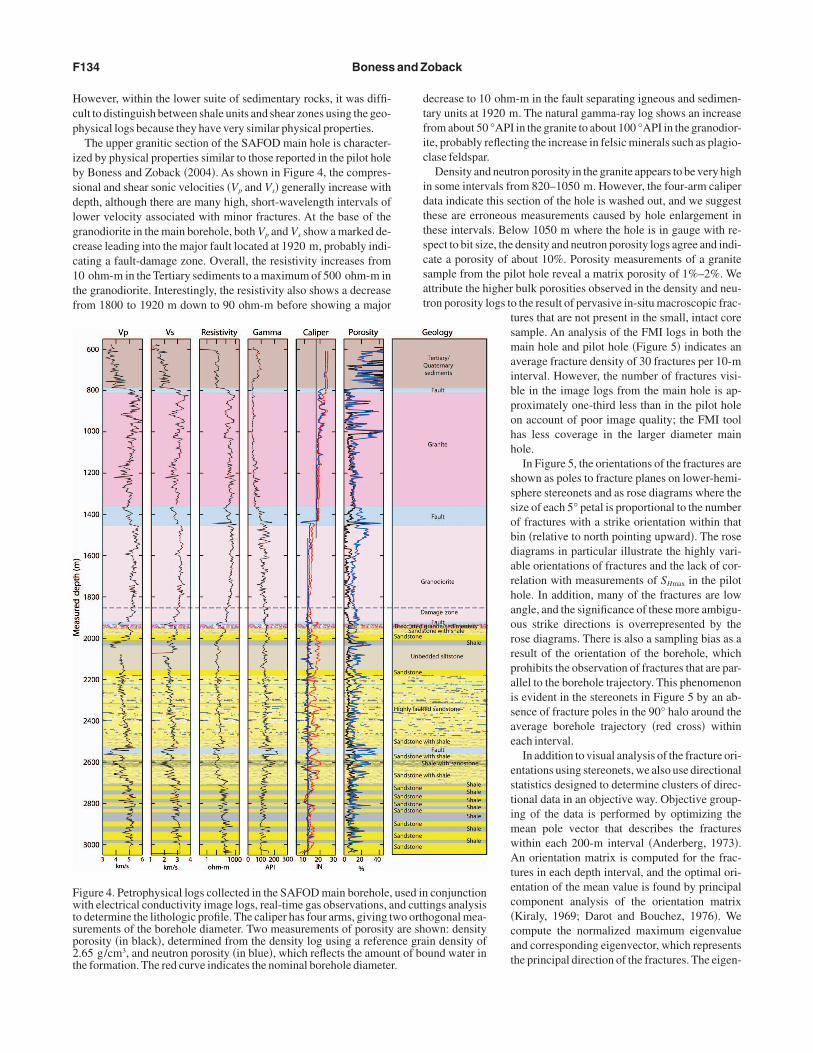
The upper granitic section of the SAFOD main hole is character-zed by physical properties similar to those reported in the pilot holey Boness and Zoback �2004�. As shown in Figure 4, the compres-ional and shear sonic velocities �Vp and Vs� generally increase withepth, although there are many high, short-wavelength intervals ofower velocity associated with minor fractures. At the base of theranodiorite in the main borehole, both Vp and Vs show a marked de-rease leading into the major fault located at 1920 m, probably indi-ating a fault-damage zone. Overall, the resistivity increases from0 ohm-m in the Tertiary sediments to a maximum of 500 ohm-m inhe granodiorite. Interestingly, the resistivity also shows a decreaserom 1800 to 1920 m down to 90 ohm-m before showing a major

igure 4. Petrophysical logs collected in the SAFOD main borehole,ith electrical conductivity image logs, real-time gas observations, a

o determine the lithologic profile. The caliper has four arms, giving turements of the borehole diameter. Two measurements of porosityorosity �in black�, determined from the density log using a refere.65 g/cm3, and neutron porosity �in blue�, which reflects the amouhe formation. The red curve indicates the nominal borehole diamete

ecrease to 10 ohm-m in the fault separating igneous and sedimen-ary units at 1920 m. The natural gamma-ray log shows an increaserom about 50 °API in the granite to about 100 °API in the granodior-te, probably reflecting the increase in felsic minerals such as plagio-lase feldspar.

Density and neutron porosity in the granite appears to be very highn some intervals from 820–1050 m. However, the four-arm caliperata indicate this section of the hole is washed out, and we suggesthese are erroneous measurements caused by hole enlargement inhese intervals. Below 1050 m where the hole is in gauge with re-pect to bit size, the density and neutron porosity logs agree and indi-ate a porosity of about 10%. Porosity measurements of a graniteample from the pilot hole reveal a matrix porosity of 1%–2%. Wettribute the higher bulk porosities observed in the density and neu-ron porosity logs to the result of pervasive in-situ macroscopic frac-

tures that are not present in the small, intact coresample. An analysis of the FMI logs in both themain hole and pilot hole �Figure 5� indicates anaverage fracture density of 30 fractures per 10-minterval. However, the number of fractures visi-ble in the image logs from the main hole is ap-proximately one-third less than in the pilot holeon account of poor image quality; the FMI toolhas less coverage in the larger diameter mainhole.

In Figure 5, the orientations of the fractures areshown as poles to fracture planes on lower-hemi-sphere stereonets and as rose diagrams where thesize of each 5° petal is proportional to the numberof fractures with a strike orientation within thatbin �relative to north pointing upward�. The rosediagrams in particular illustrate the highly vari-able orientations of fractures and the lack of cor-relation with measurements of SHmax in the pilothole. In addition, many of the fractures are lowangle, and the significance of these more ambigu-ous strike directions is overrepresented by therose diagrams. There is also a sampling bias as aresult of the orientation of the borehole, whichprohibits the observation of fractures that are par-allel to the borehole trajectory. This phenomenonis evident in the stereonets in Figure 5 by an ab-sence of fracture poles in the 90° halo around theaverage borehole trajectory �red cross� withineach interval.

In addition to visual analysis of the fracture ori-entations using stereonets, we also use directionalstatistics designed to determine clusters of direc-tional data in an objective way. Objective group-ing of the data is performed by optimizing themean pole vector that describes the fractureswithin each 200-m interval �Anderberg, 1973�.An orientation matrix is computed for the frac-tures in each depth interval, and the optimal ori-entation of the mean value is found by principalcomponent analysis of the orientation matrix�Kiraly, 1969; Darot and Bouchez, 1976�. Wecompute the normalized maximum eigenvalueand corresponding eigenvector, which representsthe principal direction of the fractures. The eigen-

conjunctionings analysisogonal mea-

own: densityin density ofund water in

used innd cuttwo orthare sh

nce grant of bor.

vprniteo

inhsjhgssspbt

twfosb

ecstw4sic

vossc2prsfrr

ftliai4

oqu

snsstntdp

iacv


ectors are described by a strike and dip, which characterizes theroperties of the fracture clusters within the interval. Eigenvaluesange from 0–1, where zero indicates complete statistical random-ess of fracture orientations and one indicates that all fractures with-n the interval have exactly the same orientation. For the fractures in-ersected by the SAFOD boreholes, the maximum eigenvalues forach interval are 0.2–0.56, indicating limited preferential directionf the macroscopic fractures.

The depth range with the most preferential orientation of fracturess 1600–2000 m in the main hole, with a fairly consistent north-orthwest strike direction. However, the same interval in the pilotole is only a lateral distance of less than 400 m away and does nothow the same consistent pattern. Below 1500 m the borehole tra-ectory is highly deviated, and the lack of consistency between main-ole orientations and the highly variable pilot-hole orientations sug-ests a sampling bias caused by the differing hole deviations. Theedimentary section was first intersected by the main hole at a mea-ured depth of 1920 m; we postulate that between 1800 and 2000 m,ome of the linear features in the FMI log inter-reted to be fractures are actually sedimentaryedding planes, explaining the degree of correla-ion in the strike direction.

The orientation of SHmax in the pilot hole as de-ermined by Hickman and Zoback �2004� usingellbore breakouts and drilling-induced tensile

ractures is also shown for reference on the stere-nets. Little correlation between the fractures andtress orientation is observed �Boness and Zo-ack, 2004�.

Below the granodiorite, the SAFOD main holencountered a sedimentary sequence of rocks,onsisting primarily of arkosic sandstones,hales, and siltstones. In general, the sonic veloci-ies are only slightly lower than those measuredithin the granite above, with Vp from.2–5.4 km/s and Vs from 2.2–3.2 km/s; bothhow an overall increasing trend with depth. Sim-larly, the resistivity in the sedimentary rocks in-reases with depth.

The gamma-ray log in the sedimentary units isery similar to the measurements within the gran-diorite and remains fairly high, which makesense, given the arkosic composition of the sand-tones that are rich in potassium feldspar and thelay-rich shales. Within some fault zones �e.g.,550 m� the gamma-ray log exhibits a local high,erhaps from an increase in clay content and en-ichment of mobile radioactive elements �potas-ium, uranium, thorium�. However, the majorault that juxtaposes granite and sedimentaryocks at 1920 m does not have a distinct gamma-ay signature.

Porosity derived from density measurements isairly consistent throughout the sedimentary sec-ion at about 10%. However, the neutron porosityog, which is sensitive to hydrous mineral phasesn addition to free water, is much more variablend increases from a background level of approx-mately 10% to a maximum of approximately0%.Although there are clear overall trends in all

Figure 5. Lowgrams of fractnitic section opilot hole andrepresent dipsare shown fortween the borfractures per 1

f the physical properties with depth throughout the sedimentary se-uence, we have identified a number of discrete sandstone and shalenits characterized by obvious deviations from average properties.

The sandstone units are characterized by higher velocities and re-istivity, low gamma-ray readings, and slightly lower density andeutron porosity values than the other sedimentary units. An analy-is of the cuttings samples in thin section reveals that these are arko-ic sandstone units, composed of angular grains of granitic originhat have been well-cemented together �D. Moore, personal commu-ication, 2005�. We discriminate bedding planes from fractures onhe FMI log by looking for intervals of very consistently striking andipping planes that are regularly spaced. The orientation of beddinglanes is shown in Figure 6.

Within the sandstones, bedding planes are observed on the FMImage log at regularly spaced intervals of 0.5–2 m. In contrast, therere many shale intervals associated with decreased velocity, de-reased resistivity, and increased gamma-ray and neutron porosityalues. In these intervals, thin-section analyses �D. Moore, personal

isphere stereographic projections of poles to fractures, and rose dia-ke determined from the electrical conductivity image logs in the gra-he pilot hole and main hole at 200-m intervals. The trajectories of theole are shown as red crosses on the stereonets, and the dashed circlesand 60° for reference. The measurements of SHmax in the pilot holece as black triangles on the rose diagrams. The lateral distance be-at each depth is also shown. The histogram depicts the number ofserved in the SAFOD main hole.

er-hemure strif both tmain hof 30°refereneholes0 m ob

c�ciccFsb

tsgisLb

2amv

td

stcbeictst

sMDw

Fsvsopa


ommunication, 2005� and X-ray diffraction analysis of the cuttingsJ. Solum, personal communication, 2005� indicate an increase inlay minerals and sheared grains relative to the sandstones. The FMImage log reveals that these intervals are also characterized by a veryonductive granular fabric with the presence of small resistivelasts. The bedding in these intervals is difficult to discern on theMI image log amid the conductive matrix; but where it is visible, ithows a much tighter spacing than the sandstone units and may beetter described as finely laminated �Figure 6�.

We interpret these intervals to be conglomeritic shale similar tohe three Cretaceous debris flow deposits found in the Great Valleyequence in the general vicinity of Parkfield. The Juniper Ridge con-lomerate is the uppermost of these channel levee units and is foundn outcrop slightly west of Coalinga, interbedded with thick-beddedandstones, mudstones, and shales �Hickson, 1999; Hickson andowe, 2002�. However, as noted above, we cannot rule out the possi-ility that some of these shale layers may be faults.

One other unit of interest is the siltstone found at approximately000 m. This siltstone is characterized by intermediate velocitiesnd resistivity but is known from drilling to contain oxidized ironinerals, causing it to be very red. The bedding in this interval, when

isible in the FMI image log, is finely laminated and reminiscent of

igure 6. Bedding planes in the sedimentary sequence between 2000ected by the main hole from electrical conductivity image log analysals. Stereonets show the poles to planes of all planar features, and roize the strike of the beds. The trajectory of SAFOD is shown with a renets, and the strike of the SAF is shown on the rose diagrams for rlot is overlain on the sedimentary lithology with a point indicating

he thin, fine-grained muddy turbidites deposited in the Great Valleyuring periods of low sediment influx �Lowe, 1972�.

In all of the units, the bedding planes strike nearly parallel to theurface trace of the SAF, and the majority dip away from the SAF tohe southwest with an average dip of 39° �Figure 6�, although in-reasingly more beds dip to the northeast near the bottom of theorehole. The opposite sense of dip �to both the southwest and north-ast� within different intervals of the sedimentary sequence mayndicate folds associated with the transpressional �simultaneous oc-urrence of strike-slip faulting and compression� nature of this tec-onic region or faults separating distinct blocks. Most of the ob-erved bedding planes are essentially perpendicular to the boreholerajectory of SAFOD.

SHEAR ANISOTROPY MEASUREDWITH DIPOLE SONIC LOGS

Data from open-hole dipole sonic shear logs are used to assesshear-wave velocity anisotropy at sonic frequencies �Kimball and

arzetta, 1984; Chen, 1988; Harrison et al., 1990�. In the pilot hole aipole Sonic Shear Imager �DSI as named by Schlumberger� logas acquired in 2002, and in the main borehole a Sonic Scanner log

�Schlumberger tool� was obtained in 2004. Thesonic scanner and DSI are multireceiver toolswith a linear array of 13 and 8 receiver stations,respectively, spaced at 6-inch intervals �Schlum-berger, 1995�. On the sonic scanner each receiverstation consists of eight azimuthal receivers; theDSI has four receivers, resulting in 104 and 32waveforms, respectively, for each dipole firingwith which to compute shear velocity anisotropy.The transmitter on these dipole sonic tools is alow-frequency dipole source operating from0.8–5 kHz frequency �Schlumberger, 1995�. Adispersive flexural wave propagates along theborehole wall with a velocity that is a function ofthe formation shear modulus. At low frequenciesthe flexural-wave velocity approximates theshear-wave velocity and in the case of SAFODhas a depth of investigation of approximately1.5 m into the formation. The flexural mode is re-corded subsequently on the array of receivers.

We define the amount of velocity anisotropy as100�Vs1–Vs2�/Vs, where Vs1 is the fast shear veloc-ity, Vs2 is the slow velocity, and Vs is the meanshear velocity. We use three quality control �QC�measures to ensure the dipole shear-wave data arereliable: �1� velocity anisotropy greater than 2%,�2� a difference of more than 50% between theminimum and maximum of the crossline energies�Esmersoy et al., 1994�, and �3� a minimumcrossline energy of less than 15% after rotatingthe waveforms into the fast and slow directions�Alford, 1986�.

Stress concentrations attributable to the pres-ence of the borehole are expected to exist aroundthe wellbore to distances of up to approximatelythree borehole radii �Jaeger and Cook, 1979�. Thedispersive nature of the flexural wave �Figure 7�is used to filter out the high frequencies corre-

000 m, inter-200-m inter-rams empha-s on the stere-ce. A tadpolep of each bed

and 3is overse diagd croseferenthe di

nd the tail pointing in the dip direction.

ssslwt

sSaohalmititcb

aacda

iopvrsdmgmw

wt�occi

traptiti1

h1fbmg

fobspme�idatcl1

Ftc


ponding to short wavelengths that sample the rocks subjected to thetress concentration around the borehole �Sinha et al., 1994�. The ob-ervations presented here are the shear velocities that correlate withow frequencies �usually less than about 2 kHz� and therefore longavelengths that penetrate deep into the formation beyond the al-

ered zone around the wellbore.In addition, borehole ovality biases the results of a shear-wave-

plitting analysis with dipole sonic logs �Leslie and Randall, 1990;inha and Kostek, 1996�. The dispersion curves of the rotated fastnd slow waveforms indicate apparent anisotropy from boreholevality when the shear-wave velocity shows no separation at eitherigh or low frequencies but demonstrates a significant split into fastnd slow velocities at midrange frequencies �Figure 7�. In theory, theack of separation between the shear velocities at low frequencies

eans that anisotropy as a result of borehole ovality would automat-cally be removed in the QC procedure described above. However, inhe main hole there are numerous examples where the caliper datandicate an enlarged hole and the shear waves do not always showypical behavior at low frequencies. By analyzing the dispersionurves at every depth interval, we could remove all cases whereorehole ovality affects anisotropy.

Also, studies show that the fast and slow dispersion curves exhibitcrossover in the presence of stress-induced anisotropy �Winkler etl., 1998�, which would provide valuable information regarding theause of the anisotropy. However, the overall quality of the SAFOData set is insufficient to assess the crossover phenomenon with anyccuracy.

DIPOLE SHEAR ANISOTROPY IN SAFOD

After applying the QC measures to the dipole sonic data collectedn the SAFOD boreholes, we project the fast polarization directionsbserved in the deviated section of the borehole onto a horizontallane so they may be compared directly with fast directions in theertical section of the borehole. We then compute the mean fast di-ection of the shear waves over 3-m intervals. We choose Binghamtatistics �Fisher et al., 1987� to compute the mean because the fastirections are of unit amplitude �i.e., they are not vectors�. The nor-alized eigenvalues �computed in the same way as for fractures�

ive a measure of the relative concentration of orientations about theean, and we discard any mean fast direction over a 3-m intervalith a normalized eigenvalue of less than 0.9.The upper vertical section of the main hole essentially overlaps

ith the pilot hole, and we choose to use the seismic velocity aniso-ropy results from the pilot hole within this depth interval700–1500 m� because the borehole is smaller and has fewer wash-uts, so the sonic tool is better centered within the hole. However, aomparison of both logs indicates a high level of repeatability. Theombined dipole sonic anisotropy results from both holes are shownn Figure 8.

Within the granite, from 760–1920 m, the fast polarization direc-ion of the shear waves is approximately north-south and exhibits aotation to a more northeasterly direction with depth. The amount ofnisotropy decreases from about 10% at the top of the granite to ap-roximately 3% at the bottom of the granodiorite. Three distinct in-ervals exist within the granite, where the amount of anisotropys observed to increase by up to 10% above the overall trend in bothhe pilot hole and the main borehole. The depths of these intervalsn the pilot hole are reported by Boness and Zoback �2004� as150–1200 m, 1310–1420 m, and 1835–1880 m. In the main bore-

ole we observe increases in the amount of anisotropy at 1050–100 m, at 1360–1455 m, and at the granodiorite-sediment inter-ace at 1920 m. It is relevant that in both the pilot hole and mainorehole, the fast polarization direction within these intervals re-ains consistent with the fast direction throughout the rest of the

ranite, even though the amount of anisotropy increases.Above a depth of 1920 m, in both the pilot hole and main hole, the

aults and fractures observed on the image logs show no preferentialrientation �Figure 5�. However, the direction of SHmax from a well-ore failure analysis in the pilot hole �Hickman and Zoback, 2004� ashown in Figure 8 illustrates the remarkable correlation between fastolarization direction and stress within the granitic section. The seis-ic anisotropy is interpreted to be stress induced, caused by the pref-

rential closure of fractures in response to an anisotropic stress stateBoness and Zoback, 2004�. Further evidence for stress-induced an-sotropy is that the amount of velocity anisotropy decreases withepth in the granite section of the borehole from approximately 10%t 780 m, to 3% at 1920 m �Figure 8�. We interpret this decrease to behe result of increased confining pressure with depth, which tends tolose fractures in all orientations and thus makes velocity anisotropyess stress sensitive at higher pressure �e.g., Nur and Simmons,969�.

The zones in the granite where the amount of anisotropy in the

igure 7. Example of dispersion curves for rotated waveforms usedo distinguish between �a� formation anisotropy and �b� anisotropyaused by borehole ovality.

swlitwewfzme

sistbwi

aswf

FcpfliSTgoantpg

Fhbih


onic log increases by up to 10% above the overall trend correlateith intervals of anomalous physical properties �e.g., low sonic ve-

ocity, low resistivity, high gamma-ray readings, increased fractur-ng�. As discussed in detail by Boness and Zoback �2004�, these in-ervals are intensely fractured but do not exhibit borehole breakouts,hich is curious, considering that the low velocity would imply low-

r rock strength. These intervals are interpreted to be shear zonesith low shear stress, probably resulting from past slip events on

aults. The high amounts of velocity anisotropy within the shearones are inferred to be the result of the increased sensitivity of seis-ic velocity at low mean stress �e.g., Nur and Simmons, 1969� or of

nhanced microcracking �Moos and Zoback, 1983�.The fact that the fast shear waves are polarized parallel to the

tress in the shear zones leads us to believe this is not structural an-sotropy but instead is related directly to perturbations in the stresstate. It is well known that fault zones are often associated with a ro-ation of SHmax and a localized absence of breakouts �Shamir and Zo-ack, 1992; Barton and Zoback, 1994�. Interestingly, we observeesterly rotations in the fast direction of the shear waves over depth

ntervals of approximately 100 m just below the major shear zones

igure 8. Observations of shear velocity anisotropy from the dipole sole �700–1500 m� and main hole �1500–3050 m�. The directionedding planes �red dashed line� is the mean strike determined in the ety image. The black bars in the middle plot indicate the orientationole.

t 800, 1400, and 1920 m. The rotation in fast directions is below thehear zones, whereas the gradual change in physical properties thate interpret to be a damage zone appears to lead into the shear zones

rom above.At the transition from granite to sedimentary lithology at 1920 m,

igure 8 illustrates that the amount of velocity anisotropy signifi-antly increases to an average value of about 6%, which remains ap-roximately constant to the bottom of the hole but has a number ofuctuations on the order of ±2%. The change in lithology from gran-

te to sedimentary rocks occurs just below the depth at which theAFOD borehole begins deviating toward the San Andreas fault.his presents an obvious challenge for separating out the effects ofeology and well slope on the anisotropy and is one of the objectivesf this paper. Within the sedimentary section �1920–3000 m�, therere two trends in the fast polarization directions of the shear waves: aorthwest orientation �red dots on Figure 8� and a northeast orienta-ion �blue dots� consistent with the fast directions in the granitic up-er section. We correlate the fast polarization directions with litholo-y and petrophysical properties and model the observations of shear

anisotropy, taking into account the borehole devi-ation and the orientation of the formation beddingplanes. In many places, the orientation of the bed-ding planes is nearly orthogonal to the wellbore;however, if the bedding planes were exactly per-pendicular, then no structural anisotropy wouldbe detectable. Thus, even though the amount ofanisotropy may be diminished with this geome-try, if any anisotropy is observed, the fast azimuthof the shear waves still contains useful informa-tion about the formation. We propose that bothstress and lithologic structure are dominant con-trols on the anisotropy we observe.

To further our understanding of the structuralanisotropy within the sedimentary section, weconsider the FMI log from 2000–3000 m in dis-crete intervals of 10 m and compute the mean bedorientation �dip direction and strike� using Fishervector distribution statistics �Fisher et al., 1987�.We discard all intervals with less than four beds orwith a normalized mean eigenvalue of less than0.9. After computing the mean bed orientations,we use the theoretical formulation in Appendix Ato compute the apparent fast direction for eachdiscrete 10 m interval that would be observed inthe SAFOD borehole if the shear waves were be-ing polarized with a fast direction parallel to thebedding planes. Between 2000 and 3000 m, theborehole has an average azimuth and deviationfrom vertical of 35° and 54°, but a gyroscopic sur-vey is used to input the exact borehole azimuthand inclination at each depth interval. In Figure 9we show the number of bedding planes used tocompute the mean orientation and compare thetheoretical apparent fast direction with the fast di-rection observed on the dipole sonic tool.

Figure 9 shows that within the well-cemented�high seismic velocity�, massively bedded sand-stones �2170–2500 m�, the sonic log exhibits anortheast fast polarization direction, consistentwith observations in the granite at shallower

gs in the pilotsedimentary

al conductiv-ax in the pilot

onic loof thelectricof SHm

difitlpsmlstsws

ssgs1ft1i

c5oacemododovlSvls

tlrehpacoTet7

cvacfgBt2fi

nZosirpbtat


epths but which do not correlate with the theoretical fast directionsf bedding planes were polarizing the shear waves. However, in thenely laminated, clay-rich shale and siltstone units below 2550 m,

he northwest fast direction of the sonic shear waves generally corre-ates well with the theoretical fast directions for structural anisotro-y. We interpret the seismic anisotropy within these finely beddedtratigraphic layers to be controlled by the alignment of clay andica platelets in the strike direction of the bedding planes. The FMI

og indicates that the bedding within most of the sandstone units ispaced at much larger intervals — about �0.5–2 m�. The spacing ofhese bedding planes is comparable to the 1.5 m wavelength of theonic waves at the low frequencies of interest, which explains whye only observe structural anisotropy within the shale despite the

ubparallel bedding planes present within all sedimentary units.The lack of correlation between the theoretical predictions for

tructural anisotropy and the observations in the well-cementedandstones suggests stress-induced anisotropy in these units. Theeometry of the borehole relative to the maximum compressivetress will dictate the amount of anisotropy observed �Sinha et al.,994�. The fast direction is found by rotating the sonic-log wave-orms until the maximum and minimum energy levels are found athe time of the shear wave’s arrival �Alford, 1986; Esmersoy et al.,994�, so the accuracy of the measurement is diminished when theres less anisotropy.

Assuming the observed anisotropy occurs be-ause SHmax preferentially closes fractures, the4° inclination of SAFOD will reduce the amountf stress-induced anisotropy observed by up topproximately 50% �Sinha et al., 1994�. Ofourse, this depends on the magnitudes of the oth-r two principal stresses. However, in the sedi-entary section of SAFOD, the observed amount

f anisotropy exceeds 4%, so we believe the fastirection is a robust measurement. We cannot ruleut that some of the anisotropy observed in theeviated section of the borehole is partly a resultf fractures being closed preferentially by theertical stress Sv. However, the plane perpendicu-ar to the borehole is at approximately 45° to bothHmax and Sv. But because this is a strike-slip/re-erse stress regime, SHmax is larger, and it is un-ikely that Sv is a dominant stress polarizing thehear waves.

PILOT-HOLE ARRAY

In 2002, an array of 32 3-C, 15-Hz seismome-ers was installed in the granitic portion of the pi-ot hole between 850 and 2050 m depth �Chavar-ia et al., 2004�. Data from this array are well suit-d for a shear-wave-splitting analysis because theigh sampling frequency �2 kHz� allows us toick the onset of the shear waves accurately. Wenalyze seismograms from nine local mi-roearthquakes at the 25 seismometers that wereperational in the pilot hole during the events.he earthquakes analyzed in this study are locat-d on the SAF approximately 1.5 km laterally tohe northeast and between depths of 2.7 and.3 km �Figure 10�. The events were chosen be-

Figure 9. Histcompute the mfast directionsbe observed athe lithology.

ause they had particularly well-constrained relocations �J. A. Cha-arria, personal communication, 2005�, were distributed laterallylong a limited 4-km along-strike section of the SAF, and had espe-ially high S/N ratios with impulsive shear-wave arrivals. The wave-orms used in this study arrived at the array receivers at incidence an-les of less than 40° within the shear-wave window �Nuttli, 1961;ooth and Crampin, 1985�, minimizing the likelihood of contamina-

ion from converted phases. The shear-wave energy peaked at0 Hz, so we filtered the seismograms using a Butterworth bandpasslter with 5–35-Hz limits.The shear-wave-splitting analysis was conducted using a tech-

ique that combines the methods of Silver and Chan �1991� andhang and Schwartz �1994�. We used a grid search to find the valuesf fast polarization direction and the time delay between the splithear waves that best corrected the seismograms for the effects of an-sotropy. The recorded seismograms were rotated into an earthquakeeference frame, the particle motion of the SH and SV waveforms waslotted on a hodogram, and the shear-wave arrival was determinedy looking for an abrupt change from linear to elliptical particle mo-ion. The seismograms were windowed around the shear-wave arriv-l with 0.2 s before the shear-wave arrival and 0.5 s after. For or-hogonal shear-wave displacement vectors u1 and u2 �usually direc-

showing the number of bedding planes per 10-m interval used toed orientation using Fisher statistics, and comparison of observedhe sonic logs with the theoretical apparent fast direction that wouldg the fast direction is oriented along the bedding planes, overlain on

ogramean bfrom t

ssumin

tt

wsotn=epm1

Wtopwtg�s

cem

ftatmcat

slawodaasatrt1vid

Fw


ions 1 and 2 refer to north-south and east-west�, the covariance ma-rix of the particle motion is computed by

cij��,�t� = �−�

�

ui��t�uj

��t − �t�dt i, j = 1,2, �1�

here ul� indicates a horizontal rotation of ul by � degrees. We

earched over values of � in 1° increments from −90° to 90° andver delay times �t between 0 and 50 ms in increments of the dataime sampling interval of 0.05 ms. If anisotropy existed, cij had twoonzero eigenvalues �1 and �2, where �1 was the largest �unless �n�/2 for n = 1,2...�. The fast direction and delay time that best lin-

arized the particle motion were determined by minimizing �2 of thearticle motion covariance matrix. To quantify the accuracy of theeasurement, we computed the degree of rectilinearity �Jurkevics,

988� as

r = 1 − ��1

�2� . �2�

e only reported measurements with a degree of linearity greaterhan 0.8 �1 being perfectly linear�. Once rotated into a fast-slow co-rdinate system, the fast and slow waveforms should have similarulse shapes. Following the method of Zhang and Schwartz �1994�,e confirmed the fast polarization direction and more accurately de-

ermined the delay time by crosscorrelating the windowed seismo-rams at each rotation step over lags of ±0.2 s. Silver and Chan1991� point out that maximizing the crosscorrelation coefficient isimilar to minimizing the determinant, so we used the maximum

igure 10. Diagram drawn to scale, showing the pilot-hole array and tith approximated linear raypaths to �a� lower and �b� upper receiver

rosscorrelation coefficient to confirm the seismograms were rotat-d into the fast and slow polarization directions. We discarded anyeasurement that had a crosscorrelation coefficient of less than 0.7.To ensure the highest level of confidence, we only reported the

ast polarization direction from the covariance matrix decomposi-ion if the maximum crosscorrelation coefficient were for a rotationzimuth within ±10° of this measurement. The maximum uncertain-y on the fast polarization directions was therefore estimated to be a

aximum of ±10°. The time delay we documented was from therosscorrelation procedure and was normalized by the distancelong a linear raypath from the source to the receiver.An example ofhe shear-wave-splitting analysis procedure is shown in Figure 11.

The results of this study using data from the pilot-hole array arehown in Figure 12, plotted at the depth of each receiver. The fast po-arization directions are north-northeast in the upper receivers on therray; but below a depth of 1400 m, the fast direction of the shearaves rotates to a northwest orientation. The northeast fast directionbserved on the upper receivers corresponds with delay times thatecrease with depth from 8 ms/km at the top of the array to 4 ms/kmt 1400 m. The fast directions determined on the upper receiverslso correlate with the direction of SHmax determined in the pilot-holetress analysis �Hickman and Zoback, 2004�. The decrease in themount anisotropy is consistent with stress-induced anisotropy ashe confining pressure increases with depth. The northwest fast di-ection observed on the lower receivers is associated with delayimes that show an apparent increase with depth from 4 ms/km at400 m up to about 10 ms/km at 2000 m. The observations of shearelocity anisotropy on the lower receivers of the pilot-hole array arenconsistent with stress-induced anisotropy, but the fast polarizationirections correlate with the fabric of the sedimentary bedding. The

deeper on the array a receiver is, the more relativetime the seismic waves spend being polarized bythe fault fabric, which accounts for the increasingdelay time with depth.

We contend that on these lower receivers, weare observing structural anisotropy. However, itis not intuitive how shear waves generated by asingle earthquake can display both stress-inducedanisotropy and structural anisotropy at differentreceivers in the same vertical array. To explainthis apparent paradox, we show simplified �i.e.,linear� raypaths from the nine earthquakes ana-lyzed to both an upper and a lower receiver in Fig-ure 10. Raypaths to the lower receivers are mostlythrough the northwest-striking sedimentary bed-ding, explaining the presence of structural aniso-tropy observed on the lower receivers. Of course,the depth extent of the sedimentary package is un-constrained, so it is very possible that the lower-most raypaths are also entirely in the sediments.However, it is well known that the amount of an-isotropy is cumulative along the raypath but thatthe polarization direction is controlled by the lastanisotropic medium encountered by the wave�e.g., Crampin, 1991�. Thus, the lower raypaths,which are in the sediments immediately beforebeing recorded, are polarized by the bedding.

The raypaths to the upper receivers also gothrough the sedimentary sequence, but the lastportion of the raypaths is through the fractured

earthquakesarray.

he nines in the

Ss

tsWato

s�Sds7ftir

eS1fnotmaps

iiasvotr2sbl

Ftsicar

Fcss


alinian granite above the sedimentary section, giving rise to the ob-erved stress-induced anisotropy.

DISCUSSION

The separation of stress-induced and structural anisotropy usinghe formulation in Appendix A allows us to supplement existingtress data in the crust surrounding the SAF in Parkfield, California.

ithin the sandstone units, where we have modeled stress-inducednisotropy, the fast polarization directions in the sonic logs indicatehat SHmax is 0°–45° �north to northeast� within a few hundred metersf the active fault plane. This correlates well with observations of

igure 11. Example of the shear-wave-splitting procedure for one ofhe nine earthquakes to one of the receivers, showing �a� the originaleismograms rotated into an earthquake reference frame, �b� the hor-zontal waveforms rotated into the fast and slow directions with theorresponding elliptical particle motion plot indicating anisotropy,nd �c� the fast and slow seismograms and particle motion plot cor-ected for anisotropy.

tress from borehole breakouts and tensile cracks in the pilot holeHickman and Zoback, 2004�, which show a clockwise rotation ofHmax with depth, indicating increasing fault-normal compressioneeper in the crust adjacent to the SAF. The results from this analysisupport that interpretation, with SHmax estimated to be at an angle of0° to the strike of the SAF at a vertical depth of 2500 m. We there-ore infer the continuation of fault-normal compression to the bot-om of the borehole within 200 m lateral distance of the SAF. Thismplies that the SAF is indeed a weak fault that slips at low levels ofesolved shear stress.

Models to explain the weakness of the SAF are abundant in the lit-rature �e.g., Sibson, 1973, 1992; Byerlee, 1990, 1993; Rice, 1992;leep and Blanpied, 1992; Brune et al., 1993; Sleep, 1995; Miller,996; Melosh, 1996� and include frictionally weak materials in theault core, high pore pressure that reduces the normal stress, and dy-amic weakening mechanisms. However, the significance of manyf the models cannot be evaluated because of the uncertainty abouthe physical properties of the fault zone and the absence of direct

easurements of the state of stress, porosity, and permeability. Wenticipate that data collected in SAFOD across the fault zone inhase two of drilling will significantly improve our current under-tanding of the faulting mechanics and strength of the SAF.

Our observations of shear velocity anisotropy at multiple scalesllustrate the effect of frequency and scale. Seismic waves are polar-zed only if the smallest wavelength is much larger than the individu-l layer thicknesses �Backus, 1962; Berryman, 1979�. The dipoleonic logs acquired within SAFOD correspond to wavelengths of in-estigation on the order of 1.5 m and are subsequently polarizednly by the sedimentary bedding in the finely laminated shale whenhe bedding planes are closely spaced. In contrast, the seismogramsecorded on the pilot-hole array from earthquakes approximately–4 km away exhibit structural anisotropy for raypaths through theedimentary sequence, since both the shale and the sandstones haveedding planes at a much closer spacing than the seismic wave-engths of approximately 30 m.

igure 12. Results from shear-wave-splitting analysis of nine mi-roearthquakes recorded on the pilot-hole array. The strike of theedimentary bedding planes and the orientation of SHmax are alsohown for reference.

ttiattfivwppl

il1cpfvstoo

sfwrststttsf

sadabtwahstr

tecvt

ifdrisdtlbaefim

sfspsweiebvaslssh

strrstc

abpcaAtmmqs

dtfr


The frequency dependence of anisotropy has important implica-ions for the scale length of heterogeneities and in establishing rela-ionships between fractures and permeability anisotropy. Interest-ngly, the frequency of investigation has a significant effect on themount of velocity anisotropy. In the sonic log the amount of veloci-y anisotropy ranges from 2%–10%, whereas at seismic frequencieshe amount of anisotropy is 1%–5%. This is in direct contrast to thendings of Liu et al. �2003�, who observe a decrease in the amount ofelocity anisotropy as the frequency increases for identical shear-ave paths. However, the sonic and seismic waves in this study sam-le very different volumes of the crust, and the geometry of the ray-aths with respect to the formation symmetry axes differ significant-y for our sonic and seismic experiments.

Within the sedimentary sequence the lithologic effect on the an-sotropy is important at the two different scales. The amount of ve-ocity anisotropy is usually 1%–4% for most rocks below a depth of–2 km �Crampin, 1994�. However, shales, clays, and mudstonesan induce a lithologically controlled anisotropy of several tens ofercent. The reason we observe an increase in anisotropy at higherrequencies may be because the sonic waves are traveling over smallolumes of highly anisotropic rock associated with the clay-richedimentary layers and/or shear zones. The lower amount of aniso-ropy at seismic frequencies recorded on the pilot hole reflects a lossf resolution because the larger wavelengths average the propertiesf the anisotropic layers over tens of meters.

In the Parkfield region, the crust is anisotropic as a result of bothtress and structure, which act as competing mechanisms.At seismicrequencies, the shear waves are affected by structural anisotropyithin the sedimentary sequence, but the polarity of the time delay is

eversed because the waves also travel through the granite/sand-tones where stress-induced anisotropy is dominant. The integratedime delays from all anisotropic layers along the raypath are muchmaller than one would expect if the waves had traveled onlyhrough anisotropic layers with the same sense of delay. In contrast,he sonic logs show increased amounts of anisotropy in the sedimen-ary sequence, but the sonic waves are traveling through a muchmaller volume �with homogeneous anisotropy� and thus retain theull anisotropic signature of each lithologic unit.

In addition, the geometry of investigation plays a key role. Theeismic raypaths from the earthquakes to the pilot-hole receivers arelmost vertical and thus at an oblique angle to the sedimentary bed-ing, so the horizontal components recorded at the surface are not inprincipal direction. In contrast, the sonic logs were acquired in aorehole-formation geometry, so the recorded fast direction is closeo the true fast direction of the formation, except in the rare case inhich the borehole is exactly perpendicular to the bedding planes

nd no anisotropy is observed. In other words, the seismic studyas lower resolution because of the larger scale of investigation inuch a heterogeneous crust, and the geometry of the formation rela-ive to the raypath dictates the maximum anisotropy measured at theeceiver.

CONCLUSIONS

We have analyzed shear velocity anisotropy in the crust adjacento the SAF in Parkfield, California, using dipole sonic shear logs andarthquakes recorded on a vertical 3-C seismic array. In the graniteountry rock, the fast polarization direction of the shear waves in theertical section of the pilot hole and main hole is parallel to the direc-ion of the maximum horizontal compressive stress. We suggest this

s stress-induced anisotropy caused by the preferential closure ofractures in response to an anisotropic stress state. Our model pre-icts the fast direction observed for any arbitrary geometry of fast di-ection resulting from structure and borehole trajectory. For stress-nduced anisotropy we show that the apparent fast direction has theame azimuth as the maximum compressive stress, although the dipepends on the orientation of the borehole. In the vertical sections ofhe pilot hole and main hole, the fast direction observed in the sonicog correlates remarkably well with measurements of SHmax fromorehole breakouts, indicating stress-induced anisotropy. Themount of anisotropy in the granite decreases with depth, as expect-d for stress-induced anisotropy, because the overall increase of con-ning pressure with depth closes fractures in all orientations andakes the shear velocity of the rock less sensitive to stress.In the sedimentary sequence penetrated at depth by SAFOD, the

onic log exhibits two distinct fast shear polarizations: a northeastast direction in the sandstones and a northwest fast direction in theiltstone and shale units characterized by finely laminated, clay-richlanes. We use our model to show that in the clay-rich shale and silt-tone units, the observed fast direction is a result of the sonic shearaves being polarized along the bedding planes. In the well-cement-

d sandstones �which have physical properties similar to the gran-te�, we observe stress-induced anisotropy. Our theory allows us toxamine the importance of the geometry of the borehole relative tooth the structural �i.e., bedding� and stress-induced directions ofelocity anisotropy when interpreting sonic logs. The observation ofnortheast-southwest fast direction is in good agreement with other

tress measurements in the region �Townend and Zoback, 2004� andocally at the SAFOD site �Hickman and Zoback, 2004�. Our resultsupport the theory of a weak SAF with nearly fault-normal compres-ion at a vertical depth of 2.5 km and at a distance of only severalundred meters to the southwest of the fault.

An analysis of earthquakes recorded on the pilot-hole array ateismic frequencies reveals stress-induced anisotropy at receivers inhe top of the array and structural velocity anisotropy for raypaths toeceivers in the lower half of the array. We contend this is becauseaypaths to the upper receivers pass back through the granite, wheretress-induced anisotropy dominates and the fast polarization direc-ion observed is highly dependent on the last anisotropic medium en-ountered.

Structural anisotropy is a stronger mechanism than stress-inducednisotropy at depth, and we observe an increase in delay times atoth sonic and seismic frequencies for structural mechanisms. Inarticular, within clay-rich intervals the intrinsic anisotropy of thelay platelets gives rise to an extremely high anisotropy �up to 10%�t sonic frequencies. This may prove useful as a lithologic indicator.t seismic frequencies the amount of anisotropy is 1%–4% because

he longer seismic wavelengths average out the anisotropic effect ofany layers. In conclusion, both structural and stress-inducedechanisms control the velocity anisotropy at sonic and seismic fre-

uencies, but our observations have a strong dependence on thecale and geometry of investigation.

ACKNOWLEDGMENTS

We thank Tom Plona and Jeff Alford at Schlumberger for helpfuliscussions and comments on sonic-log acquisition and interpreta-ion. We also thank the many members of the SAFOD science teamor thought-provoking discussions. We are grateful to anonymouseviewers for their helpful comments and suggestions. This work

w0

tddsh�tmhepet

wThaottbph�m�

toida

abtipb

maptbpifblfegt

Fcoo

Ftcpoosd


as supported by National Science Foundation grant EAR-323938-001 and the Stanford Rock Physics and Borehole project.

APPENDIX A

MODELING SHEAR ANISOTROPY IN ANARBITRARILY ORIENTED BOREHOLE

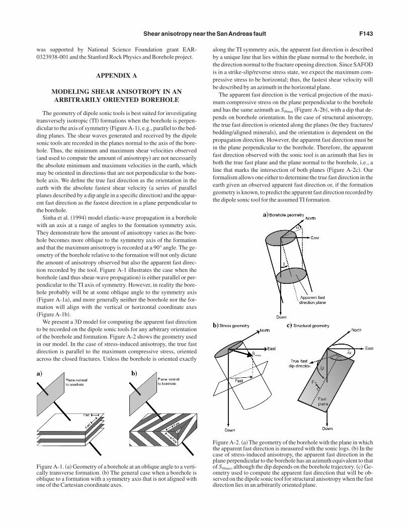
The geometry of dipole sonic tools is best suited for investigatingransversely isotropic �TI� formations when the borehole is perpen-icular to the axis of symmetry �Figure A-1�, e.g., parallel to the bed-ing planes. The shear waves generated and received by the dipoleonic tools are recorded in the planes normal to the axis of the bore-ole. Thus, the minimum and maximum shear velocities observedand used to compute the amount of anisotropy� are not necessarilyhe absolute minimum and maximum velocities in the earth, which

ay be oriented in directions that are not perpendicular to the bore-ole axis. We define the true fast direction as the orientation in thearth with the absolute fastest shear velocity �a series of parallellanes described by a dip angle in a specific direction� and the appar-nt fast direction as the fastest direction in a plane perpendicular tohe borehole.

Sinha et al. �1994� model elastic-wave propagation in a boreholeith an axis at a range of angles to the formation symmetry axis.hey demonstrate how the amount of anisotropy varies as the bore-ole becomes more oblique to the symmetry axis of the formationnd that the maximum anisotropy is recorded at a 90° angle. The ge-metry of the borehole relative to the formation will not only dictatehe amount of anisotropy observed but also the apparent fast direc-ion recorded by the tool. Figure A-1 illustrates the case when theorehole �and thus shear-wave propagation� is either parallel or per-endicular to the TI axis of symmetry. However, in reality the bore-ole probably will be at some oblique angle to the symmetry axisFigure A-1a�, and more generally neither the borehole nor the for-ation will align with the vertical or horizontal coordinate axes

Figure A-1b�.We present a 3D model for computing the apparent fast direction

o be recorded on the dipole sonic tools for any arbitrary orientationf the borehole and formation. Figure A-2 shows the geometry usedn our model. In the case of stress-induced anisotropy, the true fastirection is parallel to the maximum compressive stress, orientedcross the closed fractures. Unless the borehole is oriented exactly

igure A-1. �a� Geometry of a borehole at an oblique angle to a verti-ally transverse formation. �b� The general case when a borehole isblique to a formation with a symmetry axis that is not aligned withne of the Cartesian coordinate axes.

long the TI symmetry axis, the apparent fast direction is describedy a unique line that lies within the plane normal to the borehole, inhe direction normal to the fracture opening direction. Since SAFODs in a strike-slip/reverse stress state, we expect the maximum com-ressive stress to be horizontal; thus, the fastest shear velocity wille described by an azimuth in the horizontal plane.

The apparent fast direction is the vertical projection of the maxi-um compressive stress on the plane perpendicular to the borehole

nd has the same azimuth as SHmax �Figure A-2b�, with a dip that de-ends on borehole orientation. In the case of structural anisotropy,he true fast direction is oriented along the planes �be they fractures/edding/aligned minerals�, and the orientation is dependent on theropagation direction. However, the apparent fast direction must ben the plane perpendicular to the borehole. Therefore, the apparentast direction observed with the sonic tool is an azimuth that lies inoth the true fast plane and the plane normal to the borehole, i.e., aine that marks the intersection of both planes �Figure A-2c�. Ourormalism allows one either to determine the true fast direction in thearth given an observed apparent fast direction or, if the formationeometry is known, to predict the apparent fast direction recorded byhe dipole sonic tool for the assumed TI formation.

igure A-2. �a� The geometry of the borehole with the plane in whichhe apparent fast direction is measured with the sonic logs. �b� In thease of stress-induced anisotropy, the apparent fast direction in thelane perpendicular to the borehole has an azimuth equivalent to thatf SHmax, although the dip depends on the borehole trajectory. �c� Ge-metry used to compute the apparent fast direction that will be ob-erved on the dipole sonic tool for structural anisotropy when the fastirection lies in an arbitrarily oriented plane.

�

a

woth=

bwdpcrah

A

A

A

Fc9 t circle


As shown in Figure A-2a, for a borehole with azimuth from northand inclination from the vertical I, the vector bn, which defines the

xis of the borehole from an arbitrary origin, is given by

bn = �sin��1 + �sin��

2− I��2

�cos��1 + �sin��

2− I��2

− sin��

2− I�� ,

�A-1�

here all angles are in radians. Given the dip fd and dip direction f�

f the true fast plane, we compute three discrete points f1, f2, and f3 inhe fast plane that has a corner at the origin used to define the bore-ole. The normal to the fast plane, fn, may now be computed using af − f and b = f − f , thus giving f = a � b. The vector fa that

igure A-3. Model results for the arbitrary case of a borehole with alined at 45° �shown as a triangle on the stereonets� for four true fast0°, 180°, and 270° at a full range of dips from 0°–90° �shown as grea

1 2 2 3 n

describes the apparent fast direction fad �defined

to be in the dip direction� and the apparent fast dipfa

� from the origin are then found by computingthe line perpendicular to the borehole and to thenormal to the fast plane �i.e., in the fast plane�such that fa = bn � fn.

Figure A-3 shows the results of this computa-tion for the arbitrary case of a well with an azi-muth of 45° �i.e., northeast� and an inclination of45°. We show the apparent fast direction and dipthat will be measured in the borehole for true fastdirections dipping to the north, east, south, andwest �i.e., 0°, 90°, 180°, and 270°� over a range oftrue fast dip angles from horizontal to vertical�i.e., 0°–90°�. Typically the azimuth of the fast di-rection is reported �as a direction between −90°west and 90° east�, but the dip of the fast directionis omitted because only vertical TI symmetry isconsidered. However, given the orientation of theborehole, the dip of the apparent fast direction canbe computed easily because the observed azimuthlies in a plane normal to the borehole. For com-pleteness we present both the azimuth �as an an-gle between 180° and 180° in the direction of dip�and the dip of the apparent fast direction. We alsoshow that the dip of the fast azimuth providesvaluable information about the true orientation ofthe fast direction within the formation.

Figure A-3 illustrates the strong dependencethat the relative geometry of the borehole and truefast direction �shown here as a bedding plane�have on the apparent fast direction. In this exam-ple with a northeast-trending borehole, one cansee that if the beds dip to the north, the apparentfast direction will be southwest. However, if thebeds dip to the east, the apparent fast direction issoutheast. When the bedding planes are eitherclose to horizontal or vertical, the true fast direc-tion is hard to determine from the apparent fast di-rection. Otherwise, the results from this modelingindicate that the true fast directions will give riseto a unique apparent fast direction in the borehole.

For this borehole trajectory, the dip of the true fast direction �oredding planes� has the biggest effect on the apparent fast directionhen the beds are dipping to the south and west, i.e., away from theirection of penetration. The true fast direction is most closely ap-roximated by the apparent fast direction when the formation axis islose to being perpendicular to the borehole. This corresponds to theesults of Sinha et al. �1994�, showing the amount of anisotropy willlso be at a maximum when the formation axis is normal to the bore-ole.

REFERENCES

lford, R. M., 1986, Shear data in the presence of azimuthal anisotropy: 56thAnnual International Meeting, SEG, ExpandedAbstracts, 476–479.

lmeida, R., J. Chester, T. J. Waller, and D. Kirschner, 2005, Lithology andstructure of SAFOD Phase I core samples: EOS, Transactions of theAmer-ican Geophysical Union, 86, T21A–0454

nderberg, M. R., 1973, Cluster analysis for applications: Academic Press,Inc.

uth of 45° in-ections of 0°,s�.

n azimdip dir

B

B

B

B

B

B

B

B

B

—

C

C

C

—

—

C

D

E

F

H

H

H

H

H

J

J

J

K

K

L

L

L

L

L

L

M

M

M

M

M

M

—

N

N

R

R

S

S

S

S

—

S

S

S

S

S

TT

—

W

W


ackus, M., 1962, Long-wave elastic anisotropy produced by horizontal lay-ering: Journal of Geophysical Research, 67, 4427–4440.

akun, W. H., and T. V. McEvilly, 1984, Recurrence models and Parkfield,California earthquakes: Journal of Geophysical Research, 89, 3051–3058.

arton, C. A., and M. D. Zoback, 1994, Stress perturbations associated withactive faults penetrated by boreholes: Possible evidence for near-completestress drop and a new technique for stress magnitude measurement: Jour-nal of Geophysical Research, 99, 9373–9390.

erryman, J. G., 1979, Long-wave elastic anisotropy in transversely isotro-pic media: Geophysics, 44, 897–917.

oness, N. L., and M. D. Zoback, 2004, Stress-induced seismic velocity an-isotropy and physical properties in the SAFOD pilot hole in Parkfield, CA:Geophysical Research Letters, 31, L15S17.

ooth, D. C., and S. Crampin, 1985, Shear-wave polarizations on a curvedwavefront at an isotropic free-surface: Geophysical Journal of the RoyalAstronomical Society, 83, 31–45.

rune, J. N., T. L. Henyey, and R. F. Roy, 1969, Heat flow, stress, and rate ofslip along the San Andreas fault, California: Journal of Geophysical Re-search, 74, 3821–3827.

rune, J. N., S. Brown, and P. A. Johnson, 1993, Rupture mechanism and in-terface separation in foam rubber models of earthquakes: A possible solu-tion to the heat flow paradox and the paradox of large overthrusts: Tectono-physics, 218, 59–67.

yerlee, J., 1990, Friction, overpressure and fault normal compression: Geo-physical Research Letters, 17, 2109–2112.—–, 1993, Model for episodic flow of high-pressure water in fault zonesbefore earthquakes: Geology, 21, 303–306.

havarria, J. A., P. E. Malin, and E. Shalev, 2004, The SAFOD pilot holeseismic array: Wave propagation effects as a function of sensor depth andsource location: Geophysical Research Letters, 31, L12S07.

hen, S. T., 1988, Shear-wave logging with dipole sources: Geophysics, 53,659–667.

rampin, S., 1986, Anisotropy and transverse isotropy: Geophysical Pros-pecting, 34, 94–99.—–, 1991, Wave propagation through fluid-filled inclusions of variousshapes: Interpretation of extensive dilatancy anisotropy: GeophysicalJournal International, 107, 611–623.—–, 1994, The fracture criticality of crustal rocks: Geophysical Journal In-ternational, 118, 428–438.

rampin, S., and J. H. Lovell, 1991, A decade of shear-wave splitting in theearth’s crust, What does it mean? What use can we make of it? And whatshould we do next?: Geophysical Journal International, 107, 387–407.

arot, M., and J. L. Bouchez, 1976, Study of directional data distributionsfrom principal preferred orientation axes: Journal of Geology, 84,239–247.

smersoy, C., K. Koster, M. Williams, A. Boyd, and M. Kane, 1994, Dipoleshear anisotropy logging: 64th Annual International Meeting, SEG, Ex-pandedAbstracts, 1139–1142.

isher, N. I., T. Lewis, and B. J. J. Embleton, 1987, Statistical analysis ofspherical data: Cambridge University Press.

arrison, A. R., C. J. Randall, J. B. Aron, C. F. Morris, A. H. Wignall, and R.A. Dworak, 1990, Acquisition and analysis of sonic waveforms from aborehole monopole and dipole source for the determination of compres-sional and shear speeds and their relation to rock mechanical propertiesand surface seismic data: Annual Technical Conference and Exhibition,Society of Petroleum Engineers, Paper 20557.

ickman, S., and M. D. Zoback, 2004, Stress orientations and magnitudes inthe SAFOD pilot hole from observations of borehole failure: GeophysicalResearch Letters, 31, L15S12.

ickson, T. A., 1999, A study of deep-water deposition: Constraints on thesedimentation mechanics of slurry flows and high-concentration turbiditycurrents, and the facies architecture of a conglomeratic channel-overbanksystem: Ph.D. dissertation, Stanford University.

ickson, T. A., and D. R. Lowe, 2002, Facies architecture of a submarine fanchannel-levee complex: Juniper Ridge conglomerate, Coalinga, Califor-nia: Sedimentology, 49, 335–362.

ornby, B. E., 1998, Experimental laboratory determination of the dynamicelastic properties of wet, drained shales: Journal of Geophysical Research,103, 29945–29964.

aeger, J., and N. G. W. Cook, 1979, Fundamentals of rock mechanics, 3rded.: Chapman & Hall.

ohnston, J. E., and N. I. Christensen, 1995, Seismic anisotropy of shales:Journal of Geophysical Research, 100, 5991–6003.

urkevics, A., 1988, Polarization analysis of three-component array data:Bulletin of the Seismological Society ofAmerica, 78, 1725–1743.

imball, C. V., and T. M. Marzetta, 1984, Semblance processing of boreholeacoustic array data: Geophysics, 49, 264–281.

iraly, L., 1969, Statistical analysis �orientation and density�: GeologischeRundshau, 59, 125–151.

achenbruch, A. H., and J. H. Sass, 1980, Heat flow and energetics of the SanAndreas fault zone: Journal of Geophysical Research, 85, 6185–6223.

eslie, H. D., and C. J. Randall, 1990, Eccentric dipole sources in fluid-filledboreholes: Experimental and numerical results: Journal of the AcousticalSociety ofAmerica, 87, 2405–2421.

iu, E., S. Crampin, J. H. Queen, and W. D. Rizer, 1993, Behavior of shearwaves in rocks with two sets of parallel cracks: Geophysical Journal Inter-national, 113, 509–517.

iu, E., J. H. Queen, X.-Y. Li, M. Chapman, H. B. Lynn, and E. M. Chesnok-ov, 2003, Analysis of frequency-dependent seismic anisotropy from amulticomponent VSPat Bluebell-Altamont field, Utah: Journal ofAppliedGeophysics, 54, 319–333.

owe, D. R., 1972, Implications of three submarine mass-movement depos-its, Cretaceous, Sacramento Valley, California: Journal of SedimentaryPetrology, 42, 89–101.

ynn, H. B., and L. A. Thomsen, 1986, Shear-wave exploration along theprincipal axes: 56th Annual International Meeting, SEG, Expanded Ab-stracts, 473–476.eadows, M., and D. Winterstein, 1994, Seismic detection of a hydraulicfracture from shear-wave VSP data at Lost Hills field, California: Geo-physics, 57, 11–26.elosh, H. J., 1996, Dynamical weakening of faults by acoustic fluidization:Nature, 379, 601–606.iller, S. A., 1996, Fluid-mediated influence of adjacent thrusting on seis-mic cycle at Parkfield: Nature, 382, 799–802.oos, D., and M. D. Zoback, 1983, In-situ studies of velocity in fracturedcrystalline rocks: Journal of Geophysical Research, 88, 2345–2358.ount, V. S., and J. Suppe, 1987, State of stress near the San Andreas fault:Implications for wrench tectonics: Geology, 15, 1143–1146.ueller, M. C., 1991, Prediction of lateral variability in fracture intensity us-ing multicomponent shear-wave seismic as a precursor to horizontal drill-ing: Geophysical Journal International, 107, 409–415.—–, 1992, Using shear waves to predict lateral variability in vertical frac-ture intensity: The Leading Edge, 33, 29–35.

ur, A., and G. Simmons, 1969, Stress induced velocity anisotropy in rock:An experimental study: Journal of Geophysical Research, 74, 6667–6674.

uttli, O., 1961, The effect of the earth’s surface on the S wave particle mo-tion: Bulletin of the Seismological Society ofAmerica, 44, 237–246.

ice, J. R., 1992, Fault stress states, pore pressure distributions, and theweakness of the San Andreas fault, in B. Evans and T. Wong, eds., Faultmechanics and transport properties of rocks: Academic Press, Inc.,475–503.

oeloffs, E., and J. Langbein, 1994, The earthquake prediction experiment atParkfield, California: Reviews of Geophysics, 32, 315–336.

ayers, C. M., 1994, The elastic anisotropy of shales: Journal of GeophysicalResearch, 99, 767–774.

chlumberger, 1995, DSI* Dipole Shear Sonic Image: Oilfield MarketingServices, Schlumberger.

hamir, G., and M. D. Zoback, 1992, Stress orientation profile to 3.5 kmdepth near the SanAndreas fault at Cajon Pass, California: Journal of Geo-physical Research, 97, 5059–5080.

ibson, R. H., 1973, Interactions between temperature and pore-fluid pres-sure during earthquake faulting and a mechanism for partial or total stressrelief: Nature, 243, 66–68.—–, 1992, Implications of fault-valve behavior for rupture nucleation andrecurrence: Tectonophysics, 211, 283–293.

ilver, P. G., and W. W. Chan, 1991, Shear wave splitting and subcontinentalmantle deformation: Journal of Geophysical Research, 96, 16429–16454.

inha, B. K., and S. Kostek, 1996, Stress-induced azimuthal anisotropy inborehole flexural waves: Geophysics, 61, 1899–1907.

inha, B. K., A. N. Norris, and S.-K. Chang, 1994, Borehole flexural modesin anisotropic formations: Geophysics, 59, 1037–1052.

leep, N. H., 1995, Ductile creep, compaction, and rate and state dependentfriction within major fault zones: Journal of Geophysical Research, 100,13065–13080.

leep, N. H., and M. L. Blanpied, 1992, Creep, compaction and the weak rhe-ology of major faults: Nature, 359, 687–692.

homsen, L., 1986, Weak elastic anisotropy: Geophysics, 51, 1954–1966.ownend, J., and M. D. Zoback, 2001, Implications of earthquake focalmechanisms for the frictional strength of the San Andreas fault system, inR. E. Holdsworth, R. A. Strachan, J. F. Magloughlin, and R. J. Knipe, eds,The nature and significance of fault zone weakening: Geological Societyof London Special Publication, 186, 13–21.—–, 2004, Regional tectonic stress near the San Andreas fault in centraland southern California: Geophysical Research Letters, 31, L15S11.illiams, C. F., F. V. Grubb, and S. P. Galanis, Jr., 2004, Heat flow in theSAFOD pilot hole and implications for the strength of the San Andreasfault: Geophysical Research Letters, 31, L15S14.illis, H., G. Rethford, and E. Bielanski, 1986, Azimuthal anisotropy, Oc-currence and effect on shear wave data quality: 56th Annual InternationalMeeting, SEG, ExpandedAbstracts, 479–481.

W

Z

Z

Z


inkler, K. W., B. K. Sinha, and T. J. Plona, 1998, Effects of borehole stressconcentrations on dipole anisotropy measurements: Geophysics, 63, 11–17.

hang, Z., and S. Y. Schwartz, 1994, Seismic anisotropy in the shallow crustof the Loma Prieta segment of the San Andreas fault system: Journal ofGeophysical Research, 99, 9651–9661.

inke, J. C., and M. D. Zoback, 2000, Structure-related and stress-induced

shear wave velocity anisotropy: Observations from microearthquakesnear the Calaveras fault in central California: Bulletin of the SeismologicalSociety ofAmerica, 90, 1305–1312.

oback, M. D., M. L. Zoback, V. S. Mount, J. Suppe, J. P. Eaton, J. H. Healy,D. Oppenheimer, P. Reasenberg, L. Jones, C. B. Raleigh et al., 1987, Newevidence on the state of stress of the San Andreas fault system: Science,
238, 1105–1111.

a multiscale study of the mechanisms controlling shear...

Documents