A Neural-Network-Based Differential Evolution Approach for Face Recognition

Cheng-Jian Lin Department of Computer Science and Information Engineering

National Chin-Yi University of Technology, Taiwan

Chun-Cheng Peng Integrated IT Work, Taiwan

1 Introduction

Computer-vision-based intelligent systems and their applications, such as the digital surveillance sys-tems, automatic vehicle license plate recognition systems and the retina scan, have become more im-portant and attracted high attentions in recent years. Among these applications, being one of the extreme-ly difficult problems, face recognition (FR) plays a critical role, for the sakes of effected by a substantial variation in light direction, different face poses, and diversified facial expressions. As a result, FR is more challenging than face localization in which it is assumed that the image contains only one face.

In general, most of the FR approaches have focused on the use of two dimensional images. Since FR is still an unsolved problem under the different conditions, such as the pose, illumination or database size, we present an innovative method that combines two-dimensional (2D) texture and three-dimensional (3D) images surface feature vectors in this chapter.

Recently, the statistics-based methods, such as the principle component analysis (PCA) (Sun et al., 2007; Yang et al., 2007), and the independent component analysis (ICA) (Luo et al., 2008), linear dis-criminate analysis (LDA) (Guru & Vikram, 2008) and common vector method (CVM) (Zhaoa & Zoua, 2006), have been advocated for the FR problem. In these approaches, researchers utilized the pixel inten-sity or intensity-derived features and the characteristic classifier has its own representation of basis vec-tors from a high-dimensional face vector space for obtaining the corresponding features of face images. However, these methods can only analyze 2D gray images; it is not sufficient for 3D characteristic imag-es with changes by different facial expressions and poses. In order to improve the above-mentioned methods, some researchers proposed to use the depth information to detect 3D modality for the FR prob-lem.

It is known that the depth information is the explicit expression of shape and is invariant under dif-ferent lighting and facial pose conditions. Hence, it can be effective to curtail computational complexity and to decrease relative costs of image-capturing devices, such as laser range scanners and structured light scanners. There are some approaches, such as using nose information (Pan et al., 2005), mapped depth images (Lu & Jain, 2006) and shape of facial curves (Chafik & Anuj, 2006), have been proposed for the 3D FR problem. However, since the depth information is invariant under both different lighting and pose conditions, there are some to-be-tackled issues of expressional variations. Therefore, we com-bined texture- and depth- information and propose a novel method to improve identification performance for the 3D FR problem.

The Gabor wavelets are applied to extract invariant features, under conditions with different facial expressions or varying viewpoint angles, i.e., from only one stored prototype face (frontal view with neu-tral expression) per person of face feature, and to derive an augmented feature vector for FR. In the litera-ture, there are many researchers (Yuen et al., 2004; Lin & Chin, 2004; Chaari et al., 2008) applied the similar process. The efficiency of the Gabor wavelets lie under the fact that they exhibit similarity to the 2D receptive field profiles of the man visual neurons, offering spatial locality, spatial frequency and ori-entation selectivity. As the result, the Gabor-wavelet representation of facial images could be robust to illumination and facial expression variations. In this chapter, only the Gabor-wavelet filter is used to re-veal the local features. Facial textures and surface feature vectors are obtained by the PCA method, while both relative defects were compensated by combining gray and depth feature vectors.

After these above-mentioned procedures are completed for data preprocessing, in the following identification stage a specific classifier is required to further construct our intelligent FR system. Except the some special structures, most often used classifiers include fuzzy inference systems (Lin & Chin, 2004), artificial neural networks (ANNs) (Lin & Chin, 2004; Obaidat & Macchiarolo, 1994; Lacher et al., 1992; Chacon & Rivas-Perea, 2007) and fuzzy neural networks (Lin & Chin, 2004; Lin and Xu, 2007), here we adopt ANNs to perform FR.

Since ANNs can efficiently learn facial feature vectors and effectively implement rapid classifica-tion tasks via various training algorithms, we focus on this approach in this chapter. Once the neural ar-chitecture is determined, another important issue is to apply some effective and efficient algorithm to complete the given learning task, while the backpropagation (BP) algorithm (Lacher et al., 1992) is one of the most popular supervised methods, in which the error curve may converge very quickly. Unfortu-nately, the BP’s optimization process may fall into the local minimum. In order to tackle this drawback, another popular optimization algorithm, called differential evolution (DE) (Liu et al., 2007; Brest et al., 2006; Storn & Price, 1995; Storn & Price, 1997; Storn & Price, 1996), was proposed in the literature, which generally outperforms the BP algorithm. The DE method has been proven to be a promising can-didate for optimizing real-valued multi-modal objective functions. Besides its great convergence proper-ties the DE method is very simple for both understanding and implementing, as well as that its nature of being particularly easy to work with, by having only few control variables which remain fixed throughout the entire optimization procedure. As the result, in this chapter, our proposed approach consists of an ANN classifier with the DE optimization to tackle the difficult FR problem.

The rest of this chapter is organized as follows. After the data preprocessing procedures, i.e., the Gabor wavelet, wavelet transform, and PCA, are described in section 2, our proposed approach is pre-sented in section 3. Section 4 exhibits experimental results and relative discussions, while section 5 con-cludes this chapter.

2 Data Preprocessing

In this work, the InSpeck's 3D scanner is used to obtain the original facial images, while this digital 3D image camera is illustrated as in Figure 1.

Figure 1: The digital 3D image camera. Figure 2: Landmark points on a facial image.

By using the specific landmark points the facial areas from captured images can be extracted, as shown in Figure 2. These points, i.e., from L1 to L10, are chosen based on their significances to represent the characteristics of a specific face. The meaningful characteristics of these points are summarized as in Table 1.

Table 1: Landmarintsusedin3Dfaces.

After the facial areas were extracted the corresponding formed datasets are required to be normal-ized, in order to provide a generally common basis for comparison of gray and depth images, make sure that only the facial areas (i.e., above the chin regions and below the forehead regions) in captured images are collected, and reduce the relative effect of data variations. As displayed in Figure 3, a new facial sur-face is granted by removed those parts out of the range defined by the given landmark points, as shown as in Figure 3(a). Then the normalization of facial images can be carried out by its size proportional to the distance between the landmark points L1, L4, L5, L10, i.e., d1=|L4 –L5|, d2=|L1–L10|, in which the size is set to 100 pixels with both directions in this work. Since the RGB formatted colorful images are directly obtained from the capturing device, images are liable to vary under the change of color or reflec-tance properties. In order to solve this problem, the most common way is to convert the colorful images to gray ones, see Figure 3(b) as an example. The gray level then represents the brightness of images, while the brightness (Y) can be calculated by Y = 0.299R + 0.587G + 0.114B generally.

(a) (b)

Figure 3: Image pre-process procedure (a) example of a captured colourful face, and (b) re-sult after gray-level normalization.

Landmark point Name L1 Forehead L2, L3 Temple L4, L5 Cheekbone L6, L7, L8, L9 Mandible L10 Chin

2.1 Gabor Wavelets

Gabor wavelets are widely used in image processing applications (Chaari & Cabestaing, 2008). Since these wavelets achieve a good compromise between frequency and spatial resolution, they are very effi-cient for encoding image features and detecting specific image components such as edges.

In this chapter, the Gabor wavelets are applied to analyze the frequency characteristics, while the goal is to gather information from captured images in both the space and frequency domains. By apply-ing the Gabor wavelets the representative features of a specific face image can be described and an aug-mented Gabor feature vector is derived for the FR problem as well. Then the Gabor filters are used to convolve the image for capturing five scales and eight orientations in the whole frequency domains, as shown as in Figure 4(a). The corresponding outputs reveal that the powerful characteristics can produce salient local features, such as eyes, nose and mouth, when we concatenate all these features of the face image in order to derive a feature vector as in Figure 4(b). In addition, as the dimension of the Gabor fea-ture vector is relatively large, the wavelet transform (Yuen et al., 2004; Lin & Chin, 2004) is applied to decompose an image in order to reduce the dataset dimension dramatically. The Gabor wavelet is able to be stated as,

ψ u,v(z) =kumv

2

σ 2 e− ku ,v2 z 2 2σ 2

eik zu ,v − eσ2 2( ), (1)

where, σ = 2π, u represents the orientation, ν the scale and ||．|| the norm operator. The wave vector ku,v is defined as:

ku,v = kveiφu , (2)

where φu = πµ / 8 and the frequency value kv is expressed as

kv = kmax / fv, (3)

kmax the maximum frequency and f is the spanning factor between kernels in the frequency domain, with the settings of kmax = π 2 and f v = 2 .

The above-mentioned operation is of the Gabor wavelet filter, while there are five different scales and eight orientations in total for the FR problem. The Gabor kernels shown in Figure 4(a) are expressed as following, i.e.,

Ou,v(z) = I(z)*ψ u,v(z), (4)

where z = (x, y) and notation * denotes the convolution operator. By consisting of different local illumi-nations and orientation features, the outputs of the Gabor kernels can effectively represent the powerful characteristics and produce salient local features, such as eyes, nose and mouth of a given facial image. In other words, when we concatenate all these traits of a face image to derive a specific feature vector, it can be defined as that S ={Ou,v(z) || u = 0 , 1 , …, 7, v = 0 , 1 , …, 4}, and the convolution outputs are pre-sented as in Figure 4(b).

Note that, by applying the imaginary variable i stated in Eq. (1), both the real and imaginary parts can be processed. In other words, not only the similar feature districts can be found, but also the differ-ence in outside parts are able to be detected. Figure 4(c) exhibits the enhanced results.

(a) (b)

(c)

Figure 4: Combining process for both the real and imaginary parts. (a) Gaobr Wavelets of Gabor kernels at five scales and eight orientations, (b) real part of the convolution outputs in face image, and (c) resulted feature vector consisting of (a) and (b) by the Gabor transform.

2.2 Wavelet Transform

The wavelet transform (WT) has been a very popular tool for image analysis in recent years (Lin & Chin, 2004). Due to its merits the WT is easily applied to the tasks of compressing, transferring and analyzing. In the proposed approach, the WT is used to decompose an image which will be reduced dramatically into a relatively lower resolution. Precisely speaking, by applying the WT to a compressed image the decomposed sub-image can effectively reduce the corresponding computational complexity and provide the local information in both space and frequency domains, while the Fourier decomposition only sup-ports global information in frequency domain.

As exhibited in Figure 5, by wavelet decomposition an original image is divided into four sub-bands. The band LL is a coarser approximation to the original image and the bands LH and HL are re-spectively changed along horizontal and vertical directions, while the HH band indicates a higher fre-quency component of the image. In other words, this is the first-level decomposition and the whole pro-cess can be further carried out for the LL sub-band recursively. After applying a two-level wavelet trans-form, an original image is disintegrated into many sub-bands in different frequency.

Figure 5: Schematic diagram of the wavelet decomposition.

In addition, the above-mentioned process is for the general WT; while in this chapter our proposed approach is applied the HAAR-WT. Figure 6 provides an example with a 4×4 matrix and exhibits the relative result.

Figure 6: A matrix division of the high and low frequency results.

2.3 Principal Component Analysis

The principal component analysis (PCA) method (Puyat & Walairacht, 2008; Sun et al., 2007; Yang et al., 2007) is a well-known powerful technique for deriving a set of orthogonal eigenvectors, i.e., principle components, from the covariance matrix of facial images. A larger eigenvalue represents that the corre-sponding eigenvector would have better discrimination ability. Since the PCA method is a very useful feature generation and reduction tool, it has been applied extensively into both the fields of face represen-tation and face recognition.

The basic approach of the PCA is to compute the eigenvectors of the covariance matrix of the original data, and approximate them by a linear combination of the leading eigenvectors. By using the PCA procedure, the test image can be identified by firstly projecting the image onto the eigen-face space to obtain the corresponding set of weights, and then, comparing with the set of weights of the faces in the training set. The distance measurement used for the matching purpose can be a simple Euclidean ap-proach. In summary, the detailed description of the PCA can be stated as follows.

Step 1: Let (X1, X2, …, Xm) represents the N2 × m data matrix, where each Xi is one of the concatenat-ed face images from the N × N space, N2 denotes the dimension of the pixel numbers, and m the number of face images in the training set.

Step 2: Computing the mean value of all given images by,

Y =

1m

Xii=1

m

∑ . (5)

Step 3: Proceeding the projection to compute the zero mean as,

Xi = Xi −Υ, (6)

where Y is the N × N feature matrix and N the dimension of the feature vector.

Step 4: Producing the correlation matrix by

Σ = X i X i

T

i=1

N

∑ . (7)

Step 5: Doing factorization to evaluate the eigenvector by

Σφi = λφi , (8)

where φ is an orthogonal eigenvector matrix and λ a diagonal eigenvalue matrix with diago-nal elements in decreasing order (λ0 >λ1 …> λN

2-1 and λ0 = λMAX). In order to derive the ei-genvector matrix form with feature space Φ,

Φ = φ1 |φ2 | ...... |φn⎡⎣ ⎤⎦ , (9)

where 1 ≤ n≤ N2.

Step 6: Let X be a test sample whose image in the feature space is Φ.

.Tn iy X=Φ (10)

Finally, we utilize the Euclidean distance among samples as the leaning sample of the neural-network classifier. In other words, the input vector in an N2-dimensional space is reduced to a feature vector in an n-dimensional subspace.

3 Our Proposed Approach

3.1 Neural Network Classifiers

With the property of rapid processing capability and many other advantages, neural network approaches have been applied to numerous classification problems (Lin & Chin, 2004; Obaidat & Macchiarolo, 1994; Lacher et al., 1992; Fuang, 2004; Mendes et al., 2002; Goh & Tan, 1994). In this chapter, the proposed algorithm for applying neural networks in the FR problem consists of the following two steps. The first step is the PCA preprocessing, i.e., to extract feature vectors from the input facial images by the PCA method, while the PCA-extracted projection coefficients are used as symbolized features of reduced di-mensions. The second step is the proposed DE learning process for neural networks to enhance the FR performance.

As illustrated in Figure 7, a simple three-layer neural network for the 3D FR problem is applied, including m, g and n processing elements (PEs) in the input, hidden and output layers, respectively.

Figure 7: Architecture of a three-layer feed-forward neural network.

Given an input pattern x, a PE j in the hidden layer receives a net input of:

net j = hjixii=1

m

∑ . (11)

And produces an output as

z j = a(net j ) = a hjixii=1

m

∑⎛⎝⎜⎞⎠⎟. (12)

The net input for a PE i in the output layer can be then expressed as

netl = wljz jj=1

g

∑ = wljj=1

g

∑ a hjixii=1

m

∑⎛⎝⎜⎞⎠⎟, (13)

while the network output is

yl = a netI( ) = a wIjz jj=1

g

∑⎛

⎝⎜⎞

⎠⎟= a wlj

j=1

g

∑ a hjixii=1

m

∑⎛⎝⎜⎞⎠⎟

⎛

⎝⎜⎞

⎠⎟. (14)

Note that the symbol a in Eqs (12)-(14) represents a transfer function and the most general non-linear transfer function for neural networks is the sigmoid one, i.e.,

a = f (x) = 11+ e− x

. (15)

In summary, within the 3-layer neural network the number of input nodes is determined by the size of the PCA-extracted features. As the fully-connected neural architecture is chosen, one can build the neural network illustrated in Figure 7 by the mentioned definitions of Eqs. (11) – (15).

3.2 Review of the Differential Evolution Method

The DE method (Liu et al., 2007; Brest et al., 2006; Storn & Price, 1995; Storn & Price, 1996; Storn & Price, 1997) is known as a robust approach, while the initial vector populations are randomly chosen and should be able to cover the entire individuals within the given parameter space. Therefore, the DE meth-od can find the global best solution by utilizing both the distance and direction information, according to the differentiations among population.

Precisely speaking, as exhibited in Figure 8, a set of optimization parameters is called an individu-al. It is represented by a jth-dimensional parameter vector. A population consists of NP parameter vectors Xi,j, 1,2, , ,i NP= K and j denotes one generation. In other words, for each generation there will be one population only.

According to the works of Storn and Price (Storn & Price, 1995; Storn & Price, 1996), we propose a novel DE algorithm with the following four operations, i.e., mutation, crossover, evaluation, and selec-tion. It is worthy-mentioned that the DE approach is a scheme for generating trial parameter vectors. In this fashion, operations of mutation and crossover are used to generate new vectors (trial vectors), and the selection procedure then determines which of the vectors will survive into the next generation. Mutation: For each target vector, a mutant vector ν is generated according to:

vi, j+1 = Xi, j + F Xr1, j − Xr 2, j( ). (16)

where r1, r2∈{1 , 2 ,…, NP}(r1≠ r2 ≠ i) are randomly chosen and mutually different, and also different from the current index i. The constant F∈[0 , 1] is a scaling factor used to control the amplification of the differential variation (Xr1,j – Xr2,j), and NP should be set to at least 4 so that the mutation can be applied. The target vector Xi,j is the continuous member among the population.

Figure 8: Schematic diagram of the DE algorithm with NP parameter vectors.

Crossover: The target vector is mixed with the mutated vector, by using the following scheme, to yield the trial vector, i.e.,

Ui, j+1 = U1, j+1,U2, j+1,…,U D , j+1( ),

where

Ui, j+1 =

vi, j+1 if r(k) ≤ CR

Xi, j if r(k) > CR

⎧⎨⎪

⎩⎪ (17)

for k = 1 , 2 ,…, D; r(k)∈[0,1] is the jth evaluation of a uniform random generator number and CR de-notes the predefined crossover constant within the range of [0,1]. Evaluation: The mean-square-error (MSE) is used to represent the fitness values and to evaluate the per-formance of each individual, which can be defined as,

MSE = 1

NP * nOut

(Ti, j −Yi, j )2

j=1

nOut

∑ .i=1

NP

∑ (18)

Selection: A greedy selection scheme is applied, where

Xi, j+1 =

Ui, j+1, if MSE(Ui, j+1) < MSE( Xi, j );

Xi, j+1, otherwise.

⎧⎨⎪

⎩⎪ (19)

If, and only if, the trial vector Ui,j+1 yields a better cost function value than Xi,j, then Xi,j+1 is set to Ui,j+1;

otherwise, the old value Xi,j is retained.

4 Experimental Results

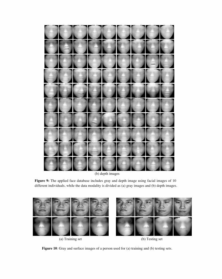
The facial image database used in this work includes 2D texture and 3D surface feature vectors, which were captured and collected from 10 different individuals by the above-mentioned InSpeck Scanner. In other words, the constructed database consists of images with gray and depth data. In the conducted ex-periments the 3D model is formed with gray and surface images. Data of each person consists of 20 faci-al images with varied poses and expressions, such as opened or closed eyes, smiling or not smiling, and normalized images with a predefined size 100*100, as exhibited in Figure 9. In addition, ten images were used for training, while the rest ten were for testing. There are two sets of experiments were conducted in this work in order to explore the effectiveness of the different variant DE methods by different input numbers of feature vectors, i.e., between 5000 and 30000 generations. Note that all the presented experi-mental results are averaged from five data-exclusive trails.

The first set of experiments for the FR problem is based on the DE algorithm described in Section 2.5, in order to evaluate the performances of the varied DE methods and the proposed approach, while Table 2 presents the numerical results and Figure 10 displays the recognition results. By increasing the number of applied eigenvectors, it is expected to have better recognition rates. Unfortunately, the compu-tational cost is growing quickly at the same time. As indicated in Table 2, individual modality under the 5000 generation is not necessarily to produce the best results. Our proposed DE method outperformed the other DE methods, i.e., standard DE/rand/1 and Variant DE/best/1. Figures 11 and 12 respectively show the results in MSEs and recognition rates, which also provide strong evidence that our proposed scheme can effectively process the FR problem with considerably great performances.

Generation = 5000

Item Standard DE/rand/1

(Storn & Price, 1995; Storn & Price, 1997)

Variant DE/best/1 (Liu et al., 2007)

Our Proposed DE/Xi,j/1

Hid Input

10 20 10 20 10 20

20 25 31 51 65 78 84 30 25 28 52 63 71 72 40 22 23 52 70 76 74 50 27 32 46 58 71 72 60 22 22 49 60 65 68

Table 2: Comparison of recognition performances for the 3D facial database (in percentage).

5 Conclusions

In this chapter, aiming at one of the difficult problems for face recognition a neural-network-based dif-ferential evolution approach is proposed. Experimental results show that by combining two modality da-ta, i.e., shape and texture facial information, our proposed approach outperforms other compared methods, in terms of better performances and higher recognition rates. Precisely speaking, when the facial angle and pose in an image are slightly changed, the adapted Gabor wavelet filter can be effectively augmented the featured representative facial images. By applying the PCA method, dimensions of feature vectors can be reduced but the recognition rate can be retained. Although it is known that the feature vectors are highly influenced by different facial poses and diversified facial expressions, our proposed approach can achieve better and much stable performance, compared to other methods. In summary, by combining both the texture and surface information, experimental results show that our proposed approach can ef-fectively enhance the FR performance, with less computational complexity.

(a) gray images

(b) depth images

Figure 9: The applied face database includes gray and depth image using facial images of 10 different individuals, while the data modality is divided as (a) gray images and (b) depth images.

(a) Training set (b) Testing set

Figure 10: Gray and surface images of a person used for (a) training and (b) testing sets.

(a) 20 features (b) 30 features

(c) 40 features (d) 50 features

(e) 60 features

Figure 11: MSE results for the 3D facial database with 10 hidden neurons and using (a) 20, (b) 30, (c) 40, (d) 50 and (e) 60 features.

(a) 20 hidden nodes (b) 30 hidden nodes

(c) 40 hidden nodes

Figure 12: Performance comparison of various DE methods by applying (a) 20, (b) 30, and (c) 40 hidden nodes.

References

Brest, J., Greiner, S., Boskovic, B., Mernik, M. & Zumer, V. (2006). Self-Adapting Control Parameters in Differential Evolution: A Comparative Study on Numerical Benchmark Problems. IEEE Transactions on Evolutionary Compu-tation, 10, 646-657.

Chaari, A., Cabestaing, F. & Sellami-Masmoudit, D. (2008). A New Approach to Face Image Coding using Gabor Wave-let Networks. In First Workshops on Image Processing Theory, Tools and Applications (pp.1-5).

Chacon, M. I. & Rivas-Perea, P. (2007). Performance analysis of the feedforward and SOM neural networks in the FR problem. In IEEE Symposium on Computational Intelligence in Image and Signal Processing (pp.313-318).

Chafik, S., Anuj, S. & Mohamed, D. (2006). Three-Dimensional FR using shapes of facial curves. IEEE Transactions on Pattern Analysis and Machine Intelligence, 28(11), 1858-1863.

Goh Y. S. & Tan, E. C. (1994). A multilayer neural network system for computer access security. In IEEE Region Ninth Annual International Conference, (pp.801-804).

Guru, D.S. & Vikram, T.N. (2007). 2D Pairwise FLD: A robust methodology for FR. In IEEE Workshop on Automatic Identification Advanced Technologies, (pp.99-102).

He, Y., Zhaoa, L. & Zoua, C. (2006). FR using common faces method. Pattern Recognition, 39(11), 2218-2222.

Huang, Y. T., Lin, C. J. & Lee, C. Y. (2007). FR Using a Modified PSO-Based Multilayer Neural Network. In 12th Con-ference on Artificial Intelligence and Applications, (pp. 168).

Juang, C. F. (2004). A hybrid of genetic algorithm and particle swarm optimization for recurrent network design. IEEE Transactions on System, Man and Cybernetics, 34(2), 997-1006.

Lacher, R.C., Hruska, S. I. & Kuncickly, D. C. (1992). Back-propagation learning in expert networks. IEEE Transactions on Neural Networks, 3(1), 62-72.

Lin, C. J. & Chin, C. C. (2004). Prediction and identification using Wavelet-based recognition fuzzy neural networks. IEEE Transactions on Systems, Man, and Cybernetics, Part B, 34(5), 2144-2154.

Lin, C. J. & Xu, Y. J. (2006). A novel genetic reinforcement learning for nonlinear fuzzy control problems. Neurocompu-ting, 69(16-18), 2078-2089.

Lin, C. J. & Xu, Y. J. (2006). The design of TSK-type fuzzy controllers using a new hybrid learning approach. Interna-tional Journal of Adaptive Control and Signal Processing, 20(1), 1-25.

Lin, C. J. & Xu, Y. J. (2007) A self-constructing neural fuzzy network with dynamic-form symbiotic evolution. Interna-tional Journal of Intelligent Automation and Soft Computing, 13(2), 123-137.

Lin, C. J., Houng, Y. T. & Lee, C. Y. (2007). A PSO-Based Modified Multilayer Neural Networks for FR. Journal of Chaoyang University of Technology, 12, 417-436.

Liu, B., Ma, H., Zhang, X. & Zhou, Y. (2007). A Memetic Co-evolutionary Differential Evolution Algorithm for Con-strained Optimization. In IEEE Congress on Evolutionary Computation, (pp. 2996-3002).

Lu, X. & Jain, A. K. (2006). Automatic feature extraction for multiview 3D FR. In 7th International Conference on Auto-matic Face and Gesture Recognition, (pp. 585-590).

Luo, B., Hao, Y., Zhang, W. & Liu, Z. (2008). Comparison Of PCA And ICA In FR. In International Conference on Ap-perceiving Computing and Intelligence Analysis, (pp. 241- 243).

Mendes, R., Cortez, P., Rocha, M. & Neves, J. (2002). Particle swarms for feedforward neural network training. In 2002 International Joint Conference on Neural Networks, (pp. 1895-1899).

Obaidat, M. S. & Macchiarolo, D. T. (1994). A multilayer neural network system for computer access security. IEEE Transactions on Systems, Man, and Cybernetics, 24(5), 806-813.

Pan, G., Han, S., Wu, Z. & Wang, Y. (2005). 3D FR using Mapped Depth Images. In 2005 IEEE Computer Society Con-ference on Computer Vision and Pattern Recognition, (pp. 175).

Puyati, W. & Walairacht, A. (2008). Efficiency Improvement for Unconstrained FR by Weightening Probability Values of Modular PCA and Wavelet PCA. In 10th International Conference on Advanced Communication Technology, (pp. 1449-1453)

Storn, R. & Price, K. (1995). Differential evolution - a simple and efficient adaptive scheme for global optimization over continuous spaces. Technical Report TR-95-012, ICSI, 1995.

Storn, R. & Price, K. (1996). Minimizing the Real Function of the ICEC’96 Contest by Differential Evolution”, In IEEE Conference on Evolutionary Computation, (pp. 842-844).

Storn, R. & Price, K. (1997). Differential evolution: a simple and efficient heuristic for global optimization over continu-ous spaces. Journal of Global Optimization, 11, 341-359.

Sun, T., Chen, M., Lo, S. & Tien, F. (2007). FR using 2D and disparity eigen-face. Expert Systems with Applications, 33(2), 265-273.

Yang, J., Zhang, D. & Yang, J. (2007). Constructing PCA Baseline Algorithms to Re-evaluate ICA-Based Face-Recognition Performance. IEEE Transactions on Systems, Man, and Cybernetics, Part B: Cybernetics, 37, 1015-1021.

Yuen, P., Dai, D. & Feng, G. (2004). FR by applying wavelet sub-band representation and kernel associative memory. IEEE Transactions on Neural Networks, 15, 166-177.

Zheng, Z., Yang, J. & Yang, L. (2005). A robust method for eye features extraction on color image. Pattern Recognition Letters, 26, 2252-2261.