a new algorithm for learning in piecewise-linear neural ...alumnus.caltech.edu/~amir/pwl.pdf ·...

A new algorithm for learning in piecewise-linear neural networks

E.F. Gada,* , A.F. Atiyab, S. Shaheenc, A. El-Dessoukid

aDepartment of Electrical Engineering, Carleton University, 1125 Colonel By Drive, Ottawa, Ont., Canada K15 5B6bDepartment of Electrical Engineering, Caltech 136-93 Pasadena, CA 91125, USA

cDepartment of Computer Engineering, Cairo University, Giza, EgyptdInformatics Research Institute, MCSRTA, Alexandria, Egypt

Received 27 June 1997; revised 15 March 2000; accepted 15 March 2000

Abstract

Piecewise-linear (PWL) neural networks are widely known for their amenability to digital implementation. This paper presents a newalgorithm for learning in PWL networks consisting of a single hidden layer. The approach adopted is based upon constructing a continuousPWL error function and developing an efficient algorithm to minimize it. The algorithm consists of two basic stages in searching the weightspace. The first stage of the optimization algorithm is used to locate a point in the weight space representing the intersection ofN linearlyindependent hyperplanes, withN being the number of weights in the network. The second stage is then called to use this point as a startingpoint in order to continue searching by moving along the single-dimension boundaries between the different linear regions of the errorfunction, hopping from one point (representing the intersection ofN hyperplanes) to another. The proposed algorithm exhibits significantlyaccelerated convergence, as compared to standard algorithms such as back-propagation and improved versions of it, such as the conjugategradient algorithm. In addition, it has the distinct advantage that there are no parameters to adjust, and therefore there is no time-consumingparameters tuning step. The new algorithm is expected to find applications in function approximation, time series prediction and binaryclassification problems.q 2000 Elsevier Science Ltd. All rights reserved.

Keywords: Neural networks; Convergence; Function approximation

1. Introduction

Neural network (NN) science has been a scene of greatactivity in recent years as its applications have flooded manydomains. In addition, there have been many advances in thehardware implementation of NN, where the digital andanalog techniques represent the main two components inthis terrain (Haykin, 1994). Continuing reduction in theworld of digital VLSI coupled with limitations in the area-reduction of analog VLSI have tempted many researchers tofocus their attention on digitally implementable NN. Inaddition to that, there are basic advantages for digital imple-mentation over that of the analog (Hammerstrom, 1992).

The sigmoidal nature of networks that make use of theerror back-propagation (BP) algorithm (Bishop, 1995)presents some difficulties for digital implementation. Theessential requirement needed for the implementation ofBP is that the backward path from the network output tothe internal nodes must be differentiable (Pao, 1989). As a

consequence, the nonlinear element, such as the sigmoid,must be continuous and that makes it difficult for digitalimplementation (Batruni, 1991). Nonetheless, digital imple-mentation of networks with nonlinear segments can becarried out by approximating the sigmoid with linearsegments and storing its derivative in a lookup table in thememory. Care should be taken to sample the region of tran-sition from linear to saturation more heavily. Naturally thismakes the memory requirement nontrivial. Although thememory requirement does not represent an acute problemas it did a decade ago, the accurate implementation of theBP requires a very large sampling. On the other hand, theanalog NN that adopt the tanh sigmoidal as their nonlinearelement also face some problems due to the crude shape ofthe “tanh” produced by the analog VLSI semiconductors,which can result in a discrepancy between the off-linetrained weights and the network on-line performance.

One way to spare us these potential troubles is to use apiecewise-linear (PWL) activity function that possesses thesmallest possible number of linear segments as the activa-tion function of the hidden neurons. However, the nondif-ferentiability of the proposed PWL NN will deprive analgorithm such as the BP of a vital requirement for proper

Neural Networks 13 (2000) 485–505PERGAMON

NeuralNetworks

0893-6080/00/$ - see front matterq 2000 Elsevier Science Ltd. All rights reserved.PII: S0893-6080(00)00024-1

www.elsevier.com/locate/neunet

* Corresponding author.E-mail addresses:[email protected] (E.F. Gad), amir@work.

caltech.edu (A.F. Atiya), [email protected] (S. Shaheen).

functioning (Pao, 1989). Approximating the derivative ofthe activation function by piecewise constant segmentswill not work easily with a BP-type scheme, since the mini-mum always occurs at the discontinuities (we have failed toachieve good results in several exploratory simulationsusing this approach). Hence, learning in PWL NN mandatessome sort of “tailored” algorithms. For example, the algorithmpresented in Lin and Unbehauen (1995) is used to trainnetworks with a single hidden layer employing the absolutevalue as the activation function of the hidden neuron. Thisalgorithm was further generalized to multilayer networks withcascaded structures in Batruni (1991). In Staley (1995), thealgorithm used adopts the incremental-type approach (orconstructive approach) for constructing a network with twohidden layers, where the hidden neurons possess a PWL func-tion in the range [0–1]. This means that one starts with aminimal network configuration and then adds more units ina prescribed manner to minimize the error. Hush and Horne(1998) proposed another incremental-type approach that usesquadratic programming to adjust the weights.

One drawback of the incremental approach is that it is notcommitted to an upper bound in the number of the networkparameters (connection weights) and can end up with largenetworks, and that generally leads to questionable general-ization performance. The intimate relationship between thenumber of the weights in the network and the generalizationperformance has been revealed in different places (see, forexample, Abu-Mostafa, 1989; Baum & Haussler, 1989;Moody, 1992).

In this paper, we studied and developed an algorithm for aclass of networks consisting of a single hidden layer and asingle output neuron. The activation function of the hiddenneurons is a PWL of the saturation type with outputs in[21,1] (see Fig. 1), whereas the output neuron possesses apure linear function. This hidden unit function has been usedin some types of Hopfield networks (Michel, Si & Yen,1991) and is called saturation nonlinearity. The proposedlearning algorithm for this class approaches the learningtask by constructing a PWL objective function for thetotal error and then seeks to minimize it. The algorithmdeveloped is a new algorithm for optimizing general PWLfunctions, and is therefore a contribution to the generaloptimization field as this path has been very scarcely trod-

den in the literature. For example, we could locate only oneidentical task, in Benchekroun and Falk (1991), where theadopted algorithm is based on the Branch and Boundscheme and defines subproblems that can be solved usinglinear programming. Our approach for PWL optimization,on the other hand, depends on utilizing the boundariesbetween the linear regions of the PWL function as thesearch directions. One of the main advantages of theproposed algorithm over BP is that it does not need anyparameters (such as the learning rate in BP)—and thereforethere is no time-consuming parameter tuning step—nordoes it use any derivative information of the error surfaceand thus can be very promising as an accelerated learningalgorithm (see Battiti, 1992). Another advantage of theproposed algorithm is that, due to the discrete nature ofthe problem, it converges in a finite number of steps, unlikeBP where the minimum is approached only asymptotically.

The proposed algorithm can be considered to belong to abroad category of algorithms called basis exchange algo-rithms, which is based on exchanging one variable withanother in a basis set. An example of a basis exchangealgorithm is the simplex algorithm for linear programming.Basis exchange algorithms have also been applied in the NNfield, for example Bobrowski and Niemiro (1984) for traininglinear classifier networks and Bobrowski (1991) for trainingmultilayer classifiers with hard-threshold neurons (thoughthese algorithms are quite different in concept from theproposed algorithm, for example Bobrowski’s 1991 algorithmis based on adding hidden nodes that are trained to maximallyseparate between one class and the remaining classes).

Besides being specifically suited for PWL NN, theproposed algorithm provides another fundamental advan-tage over gradient-type algorithms for smooth error func-tions. It is well known that if a gradient descent is used tominimize a functionQ(x), the rate of convergence becomesgoverned by the relation (Battiti & Tecchiolli, 1994;Golden, 1996):

uQ�xk11�2 Q�xp�u <hmax 2 hmin

hmax 1 hmin

� �·uQ�xk�2 Q�xp�u;

wherexp is the actual minimum,xk11 andxk are the vectorsof the independent variables at iterations�k 1 1� and k,respectively, andhmax andhmin are the largest and smallest

E.F. Gad et al. / Neural Networks 13 (2000) 485–505486

Fig. 1. The activity function of the hidden neutrons.

eigenvalues of the Hessian matrix ofQ(x). It is clear that ifthe two eigenvalues are very different (i.e. the Hessianmatrix is very ill conditioned), the distance from the mini-mum is multiplied each iteration by a number that is veryclose to 1. The problem with the NN learning is that theHessian matrix of the error function is usually ill condi-tioned. The analysis in Saarinen, Bramley and Cybenko(1993) shows why this ill conditioning is very commonwith NN learning. Our algorithm, on the other hand, is notof a gradient type and as a result is not prone to suchproblems and does not suffer from the slow rate of conver-gence as could be demonstrated by the results.

The organization of this paper is as follows. Firstly,Section 2 presents a formal terminology for describingany general PWL function. Section 3 is involved in demon-strating the basic features of the neural model considered inthis paper. The mathematical derivations of the algorithmare presented in Section 4, which consists basically of threesubsections that handle the main stages of the algorithm.Simulation results are given in Section 5 and finally Section6 presents a brief summary and conclusion.

2. Piecewise-linear functions and their representation

A complicated mapping functionf : D! RM (with D acompact subset ofRN) can be approximated through piecesof functions. A PWL function can be formally defined asfollows (Lin and Unbehauen, 1995; see also Lin andUnbehauen, 1990):

Definition 1 (PWL function). A PWL functionf : D!RM with D, a compact subset inRN, is defined from twoaspects:

1. The partition of the domainD into a set of polyhedracalled regions

�RU �Rp , Dn �� [P

p�1

�Rp � D; �Rp > �Rp0 � f; p ± p0; p;p0

[ {1 ; 2;…;P} jg1 (1)

by a set of boundaries of�N 2 1�-dimensional hyper-planesH U { Hq , D; q� 1;…;Q} ; where

Hq U { x [ Dukaq; xl 1 bq � 0} ; �2�whereaq [ RN

; bq [ R; k,l denotes the inner productoperation of two vectors andf is the empty set.

2. Local (linear) functions

f p�x� U Jpx 1 wp �3�with f �x� � fp�x� for any x [ Rp where Rp [ �R; Jp [RM×N andwp [ RM

: There have been several approaches

for describing a PWL function in a closed form (Keve-naar & Leenaerts, 1992).

Consider the caseM � 1; i.e. f : D! R: We define thefollowing:

Definition 2. A local minimum off is a connected set,�L;of points such that

f �x� � f min for x [ �L

and

f �x� . fmin for x [ �V \ �L

where �V is some open neighborhood of�L:

As a special case, an isolated local minimum is a pointx,where f �x 0� . f �x� for x 0 [ �V 2 x; where �V is an openneighborhood aroundx.

The following is a generalization of a result proved byGauss for the case of the minimization of the least absolutedeviation functionf �x� � PK

i�1 ukai ; xl 1 bi u:

Theorem 1. Let f be a PWL function defined as in Eqs. (1)and (2). If �L is a connected set of local minima off, and �L isbounded, then there is anx0 [ �L such thatx0 is the inter-section of at least N hyperplanes.

Proof. Consider the pointx0 [ �L that is the intersection ofthe largest number,K, of hyperplane boundaries, i.e.

ka1; xl 1 b1 � 0

..

.

kaK ; xl 1 bK � 0

…�x [ �L� �4�

The functionf evaluated at pointsx close tox0 that satisfyEq. (4) is linear, since there is no other hyperplane inter-secting with theK hyperplanes at pointx0 and creating adiscontinuity.

Let

x � x0 1 lx 0

wherex 0 [ :�A�;

A �

a1

a2

..

.

aK

266666664

377777775and:(A) denotes the null space ofA. If we assumeK , N;

then x 0 will be nonzero, and we can takel as large aspossible untilx hits the boundary of�L; which is anotherhyperplane. This will makex at the intersection ofK 1 1hyperplanes, which contradicts the definition ofK. Hence,the assumptionK , N is invalid, and there must be a point

E.F. Gad et al. / Neural Networks 13 (2000) 485–505 487

1 The over-bar notation denotes the closure of the set.

in �L that is at the intersection of at leastN hyperplaneboundaries. A

Corollary. An isolated local minimum is at the inter-section of at least N hyperplane boundaries (N is the dimen-sion ofx).

The above theorem is helpful in guiding the optimizationprocedure. We note that typically the minimum is at the inter-section ofN hyperplanes. It is at the intersection of more thanN hyperplanes only in case of degeneracy, such as when morethanN hyperplanes have nonempty intersection.

3. The piecewise-linear neural model

For mathematical convenience, we adopted an NN with asingle hidden layer and a single output neuron. Fig. 2 showsa schematic layout for the model. Every neuron in thehidden layer exhibits the transfer function (see Fig. 1)

fh�6� �21 6 , 21

6 1 $ 6 $ 21

1 6 . 1

8>><>>: �5�

On the other hand, the output neuron exhibits the lineartransfer function:

fo�6� � 6 �6�The output of the net,yo�m�; under the presentation of atraining examplem, drawn from a training set of sizeM,will thus be given by:

yo�m� � fo vo 1XHj�1

vj fhXI

i�1

wji ui�m�1 wjo

!0@ 1A �7�

whereui�m� is the input of examplem at the input sourcenode i, H is the number of the hidden neurons,I is thedimensionality of the input training examples,wji is theweight connecting the input nodei to the hidden neuronjandvj is the weight from the hidden neuronj to the outputneuron. Alternatively, by making use of the PWL nature ofthe hidden neuron and Eq. (6), we can write

yo�m� � vo 1X

j[SLm

XI

i�1

wji ui�m�1 wjo

!·vj 1

Xj[S1

m

vj 2X

j[S2m

vj ;

�8�whereSL

m is the set of hidden neurons activated in the linear


Fig. 2. A schematic layout for the NN model.

region upon the presentation of the examplem, i.e.

SLm U j [ {1 ;2;…;H}f j2 1 ,

XI

i�1

wji ui�m�1 wjo , 1g �9�

S1m andS2

m are the sets of hidden neurons activated in thepositive and negative saturation regions, respectively, i.e.

S1m U j [ {1 ;2;…;H}f j

XI

i�1

wji ui�m�1 wjo $ 1g �10�

S2m U j [ {1 ;2;…;H}f j

XI

i�1

wji ui�m�1 wjo # 21g �11�

From Eqs. (9)–(11), we can see thatS2m > SL

m > S1m � f and

uS2m < SL

m < S1mu � H; where u �Au denotes the cardinality of

the set �A: Taking the sum of the absolute deviations as ourcost function,E, then

E �XMm�1

uyo�m�2 T�m�u �12�

whereT(m) is the desired output for the examplem. Substi-tuting Eq. (8) into Eq. (12) we get:

E �XMm�1

sm

"vo 1

Xj[SL

m

XI

i�1

wji ui�m�1 wjo

!·vj

1Xj[s1

m

vj 2X

j[S2m

vj 2 T�m�#

�13�

wheresm is the sign of themth term between the squarebrackets. Definingw0ji � wji ·vj ; Eq. (13) can be written as

E �XMm�1

sm

"vo 1

Xj[SL

m

XI

i�1

w0ji ui�m�1 w0jo

!

1X

j[S1m

vj 2X

j[S2m

vj 2 T�m�#

�14�

It might appear that the above formulation introduces apotential problem when the optimization procedureproducesvj � 0 while w0ji ± 0: However, this problem canbe avoided by imposing the constraints:vj . e; (e is a verysmall positive constant) and thus restricting the searchregion to positivevj’s, assuming thatvj . 0 initially (anyfunction using a network with unrestrictedvj’s can also beshown to be implemented with nonnegativevj’s). Practicallyspeaking, however, these constraints turned out to degradethe efficiency of the algorithm. On the other hand, we havenot encountered any case in which such a situation hasdisturbed the algorithm, hence such constraints have notbeen enforced.

Now we can see thatE is a PWL function. Using thenotation of the previous section, we haveE : D , RN ! Rwhere everyx [ D is the vector form constituted from all

the variables appearing in Eq. (14), i.e.

xTU �w01o;…;w01I ; w02o;…;

w02I ;… …;w0Ho; …;w0HI ; vo; v1;…; vH�; (15)

and N is the total number of the weights in the network,given byN � �I 1 2�H 1 1: Thus, if we were to seek a goodminimum forE, as would stipulate any learning task in theNNs, we may search the space whose coordinates are theset of variables�w01o;…;w01I ; w02o;… ;w02I ;… …;w0Ho; …;

w0HI ; vo; v1;…; vH� instead of searching the original weightspace. Equivalently, we may refer to the variable space of(15) as the weight space. We also assume that we can definethe boundary configuration forE; � �HE� rigorously. Intui-tively, the boundary configuration�HE should have threeoutstanding types of boundaries or hyperplanes: the firsttwo types are closely similar to each other and are locatedat the two breakpoints of the activity function of each one ofthe hidden neurons, or mathematically speaking, they arelocated wherever

XI

i�1

wji ui�m�1 wjo � ^1 �16�

whereby multiplying both sides of Eq. (16) byvj enables usto formulate this boundary equation in terms of the same setof variables expressing the error functionE:

XI

i�1

w0ji ui�m�1 w0jo 2 vj � 0

m� 1;2;…;M; j � 1; 2;…;H

�17�

XI

i�1

w0ji ui�m�1 w0jo 1 vj � 0

m� 1;2;…;M; j � 1; 2;…;H

�18�

We shall refer to the boundaries in Eq. (17) as type ‘Ia’hyperplanes, denoting them byHIa

j;m; and to that of Eq.(18) as type ‘Ib’ hyperplanes (orHIb

j;m�: It is interesting tonote that the setsSL

m; S1m and S2

m exchange their membersacross these boundaries. The third type of hyperplanes orboundaries can be found wheneveryo�m� � T�m� for allm� 1;2;…;M; i.e. when themth term of Eq. (14) changesits sign:

vo 1X

j[SLm

XI

i�1

w0ji ui�m�1 w0jo

!1

Xj[S1

m

vj 2X

j[S2m

vj 2 T�m�

� 0 (19)

We shall refer to the boundaries given by Eq. (19) as type‘II’ hyperplanes orHII

m: Thus the whole set of the boundary


configuration, �HE; can be written as:

�HE U {{ HIaj;m; j [ {1 ;2;…;H} ; m

[ {1 ;2;…;M}} < { HIbj;m; j [ {1 ;2;…;H} ; m

[ {1 ;2;…;M}} < { HIIm; m [ {1 ;2;…;M}}} �20�

Evidently, it can be seen thatE is continuous across�HE;

sinceE is composed of the sum of continuous functions (theabsolute value functions).

A crucial issue regarding the type II hyperplanes shouldbe stressed here. Closer inspection of Eq. (19) reveals that ahyperplane of type II is not a strictly linear hyperplane,because by varying the weightswji, a hidden neuron canmove from the linear to the saturation region. It may berather conceived as a zigzag hyperplane with its linearsegments occurring between the types Ia and Ib hyper-planes. To illustrate better such a subtle point, consider asimple network configuration consisting of only two hiddenneurons. If a training example, sayp, is activating both ofthe hidden neurons in the linear region, i.e.SL

p �{1 ;2} ; S1

p � S2p � f; then a hyperplane of type II for the

examplep, HIIp ; would take the form

vo 1 u1�p�w011 1 u2�p�w012 1 w01o 1 u1�p�w021

1 u2�p�w0221w02o 2 T�p� � 0 (21)

Now imagine that we move in the weight space on thehyperplane of Eq. (21) until we happen to cross the bound-ary of the hyperplaneHIa

1; p ; this in fact implies that theexamplep will change its activation region of the hiddenneuron 1 to the positive saturation region. ThusHII

p becomes

vo 1 v1 1 u1�p�w021 1 u2�p�w022 1 w01o 2 T�p� � 0 �22�Now, we can see that Eq. (22) provides a different form forHII

p : The previous argument then suggests the followingstatement: a boundary associated with type II and examplem, HII

m; written as in Eq. (19) is not strictly a hyperplane. It israther zigzaggingwith its turning points occurring at itscrossings with hyperplanes of types Ia and Ib. Fig. 3 depictsa graphical illustration of this statement.

Note that the main concept of the proposed algorithm willwork as well for any PWL objective function, so for exam-ple one can add to the L1 error a penalty function such as thesum of absolute values of the weights.

4. Derivation of the algorithm

4.1. Overview of the algorithm

The algorithm consists basically of two stages: Stage-Aand Stage-B. Given a randomly chosen starting point in theweight space, the role of Stage-A is to find an intersectionpoint betweenN linearly independent hyperplane bound-aries of the error functionE. The set of these hyperplanes

will be referred to throughout the algorithm description by�H where �H , �HE: This is done by a sequence ofN steps ofsuccessive projection of the gradient direction onN hyper-planes. In each step of Stage-A, a new point is obtained,where this new point is at the intersection of one morehyperplane than the point of the previous step. Stage-A isthus terminated after exactlyN steps with the desired pointas output, which in turn serves as the starting point forStage-B.

Stage-B carries out the bulk of the optimization process.It does so by generating a sequence of points that representthe intersection ofN linearly independent hyperplaneboundaries. This is done by moving along single-dimen-sional search directions lying at the intersection of�N 21� hyperplane boundaries. The details of computing thesedirections will be explained in Section 4.3. Furthermore,Stage-B ensures that each point thus generated reduces theerror functionE. The termination point of Stage-B (and ofthe algorithm) is reached when all the available searchdirections at any one point fail to produce a point withlower error E. A theorem is also given to show that thetermination point of Stage-B is a local minimum ofE. Inaddition to that, restricting Stage-B to generate only pointsthat represent the intersection ofN hyperplane boundaries ofthe error functionE is useful according to theorem (1),because it keeps the search process more focused on thelocal minimum candidate points in the weight space.

However, the PWL nature of type II hyperplanesdescribed in the previous section could introduce some diffi-culties during Stage-B. More specifically, it is quite possiblethat Stage-B generates a point representing the intersectionof p hyperplanes wherep , N: Clearly, this situationrequires detection and/or correction. This is done by aroutine (we name it “Restore”) that is called from withinthe Stage-B procedure. This routine is based on the idea ofhypothetical hyperplanes, which is explained in Section 4.4.

4.2. Stage-A

In this stage we start randomly and then move in thedirection of the gradient descent until we hit the nearestdiscontinuity of the set�HE: The search direction is thentaken along the projection of the gradient on this hyper-plane. We continue moving in this new direction until wehit another new hyperplane belonging to the set�HE: Thusfar, we would be standing by the intersection of two hyper-planes in anN-dimensional space, or equivalently a hyper-plane of dimensionalityN 2 2; assuming that the twohyperplanes are linearly independent. We then project thedirection of the gradient on the above lesser dimensionhyperplane and move along it until we hit anothernew hyperplane. The new point obtained from the lastmovement thus represents the intersection of three hyper-planes, or in other words a hyperplane of dimensionalityN 2 3: Proceeding in the same manner, we continue untilwe reach the end of Stage-A, where the final point


represents the intersection ofN hyperplanes. Suppose that,before we reach the end of Stage-A, we happened to bestanding by the intersection ofk hyperplanes, so thatkai ; xl 1 bi � 0 (for i � 1;2;…; k� wherex is given as inEq. (15);a i andb i are a vector and a constant, respectively,that depend on the type of theith hyperplane. Or simply, inmatrix form we can write: Ax � b where, A ��a1;…; ak�T; ai � aT

i ; b � �b1;…;bk�T; bi � 2bi : Let grepresent the gradient of the error functionE, i.e.

gTU

"2E2w01o

;…;2E2w01I

;2E2w02o

;…;2E2w02I

;… …;

2E2w0Ho

;…;2E2w0HI

;2E2vo

;2E2v1

;…;2E2vH

#�23�

which can be obtained easily by checking the setsSLm; S1

m;

andS2m; and it is of course a constant vector that depends on

the region we are in. The projection of the gradient on thehyperplaneAx � b is given by

Pg � �I 2 AT�AAT�21A�g �24�hence, as discussed above, our movement fromxold to xnew

would be given according to

xnew� xold 2 hminPg �25�or assumingh � 2Pg :

w01o;new

..

.

w0HI ;new

vo;new

v1;new

..

.

vH;new

266666666666666666664

377777777777777777775

�

w01o;old

..

.

w0HI ;old

vo;old

v1;old

..

.

vH;old

266666666666666666664

377777777777777777775

1 hmin

h1

..

.

hH�I11�

hH�I11�11

hH�I11�12

..

.

hN

26666666666666666664

37777777777777777775

�26�

wherehmin is the step required to reach thenearesthyper-plane�H1a

j;m; H1bj;m; or HII

m� andhi is the ith component of thevectorh. Also note that the presence of the minus sign in thesecond term of Eq. (25) is to account for the descentdirection. To computehmin, imagine that we move

along the directionh until we hit the hyperplaneHIaj;m:

Clearly this implies that at the new point we shouldhave, using Eq. (17)

w 0j;T

newu�m�2 vj;new� 0 �27�

where w 0j;T

new� �w0jo;new;w0j1;new;…;w0jI ;new� and u�m� �

�1;u1�m�;…;uI �m��T: Substituting Eq. (27) into Eq. (26),we can obtain the step sizehIa

j;m required to reachHIaj;m;

hIaj;m U 2

�w 0j;Tu�m�2 vj�XI

i�0

ui�m�hj�I11�2I1i 2 hH�I11�111j

�uo�m� � 1�

�28�Note that in the above equation we dispensed withsubscript “old”, assuming that it is implicitly understoodthat the step size will be computed in terms of the currentvalues (the old ones). Similarly, using Eq. (18) we canobtain the step size required to reach anyHIb

j;m; along thepositive direction ofh,

hIbj;m U 2

�w 0j;Tu�m�1 vj�XI

i�0

ui�m�hj�I11�2I1i 1 hH�I11�111j

�uo�m� � 1�

�29�To determine the step size required to reach any hyper-

plane of type II for any examplem, we follow the aboveargument, where moving to a point on the hyperplaneHII

m

implies that, using Eq. (19),

vo;new 1X

j[SLm

XI

i�1

w0ji ;newui�m�1 w0jo;new

!

1X

j[S1m

vj;new2X

j[S2m

vj;new 2 T�m� � 0 �30�

Substituting from Eq. (30) in Eq. (26)

yo;old�m�1 hIIm

( Xj[SL

m

XI

i�0

ui�m�hj�I11�2I1i 1X

j[S1m

hH�I11�111j

2X

j[S2m

hH�I11�111j 1 hH�I11�11

)2 T�m� � 0

�31�whereyo,old(m) is the old output of the network for the exam-ple m before stepping ontoHII

m; hIIm is the step size alongh

that would carry us toHIIm: By ignoring the subscript “old”,

then

wheree�m� is the deviation error of the examplem

e�m� � yo�m�2 T�m� �33�

Eqs. (28), (29) and (32) define the step sizes needed to reach


hIIm U 2

e�m�Xj[SL

m

XI

i�0

ui�m�hj�I11�2I1i 1X

j[S1m

hH�I11�111j 2X

j[S2m

hH�I11�111j 1 hH�I11�11

�uo�m� � 1� �32�

any hyperplaneH [ �HE in terms of the current values of theweights. Thus, the step size that carries the search, along thepositive direction ofh, to the nearest discontinuity of the set�HE is obtained from:

hmin

� min{ minj;m

{hIaj;m . 0} < min

j;m{hIb

j;m . 0} < minm

{hIIm . 0}}

�34�

After hitting a new hyperplaneHk; this hyperplane isinserted as the newest member of the setH of satisfiedconstraints. We augment the matrixA with the row expres-sing this new hyperplane, and also augment the vectorb.Naturally, the hyperplane equationska; xl 1 b � 0 dependon its type. For hyperplanes of types Ia, Ib and II,a is given,respectively, as

aIaj;muith component

U

uk�m� i � j�I 1 1�2 I 1 k for all k � 0;…; I

21 i � H�I 1 1�1 j 1 1

0 otherwise

8>><>>:�35�

aIbj;muith component

U

uk�m� i � j�I 1 1�2 I 1 k for all k � 0;…; I

1 i � H�I 1 1�1 j 1 1

0 otherwise

8>><>>:�36�

aIImuith component

U

uk�m� i � j�I 1 1�2 I 1 k for all k � 0;…; I and allj [ SLm

21 i � H�I 1 1�1 j 1 1 for all j [ S1m

1 i � H�I 1 1�1 j 1 1 for all j [ S2m

1 i � H�I 1 1�1 1

0 otherwise

8>>>>>>>><>>>>>>>>:�37�

The constantb is given by:bIaj;m � bIb

j;m � 0; bIIm � 2T�m�.

Stage-A is terminated after exactlyN steps, or, in otherwords, when the number of the intersecting hyperplanes (thecardinality of the set�H) is equal toN. See Appendix B for adetailed pseudo code description of Stage-A. We note thatthe projection operation (Eq. (24)) need not be computedfrom scratch each new step. There are recursive algorithmsfor updating the projection matrix when adding a matrixrow. However, we will not go into these details, as wewill present a more efficient method later in the paper toeffectively perform the equivalent of Stage-A steps (seeSection 4.4).

4.3. Stage-B

After terminating Stage-A at a point representing theintersection ofN-hyperplanes, Stage-B is then initiated.We assume for now that the equations of the hyperplanesare linearly independent. At the start of Stage-B, we canwrite the following equation

a1

..

.

aN

2666437775·x �

b1

..

.

bN

2666437775 �38�

or in matrix form:Ax � b keeping in mind thatA is nowanN × N matrix; ai � aT

i ; bi � 2bi : If we let bk � bk 1 y


Fig. 3. A graphical representation for the comportment of type II hyperplanes for the examplep.

and henceb Ty � �b1…�bk 1 y�…bN� where y is a small

constant, then the new point,xy , computed fromxy �A21·by is a point representing the intersection of the follow-ing set of hyperplanes

kai ; xl 1 bi � 0 i � 1; 2;…;N i ± k �39a�

kai ; xl 1 bi � y i � k �39b�In fact, the hyperplane (39b) is not a legitimate member ofthe boundary configuration�HE; but the real gain in theabove step is that a new search direction can now beobtained using the two pointsx andxy :

h � �xy 2 x�=ixy 2 xi �40�Furthermore, the search directionh is a hyperplane of singledegree of freedom that represents the intersection of the setof N 2 1 hyperplanes of Eq. (39a). Thus, we can use thisnew search direction to resume the search process as inStage-A, where the nearest hyperplane encountered alongthe positive direction ofh, (sayH 0k; whereH 0k [ �HE; H 0k U{ x [ Duka 0k; xl 1 b 0k � 0}�; becomes the new member ofthe family of theN intersecting hyperplanes, while the oldmemberHk is dismissed. If we leta0 Tk � a 0k andb0k � 2b 0k;then the new point satisfies the system of equationsAk·x �bk; where the matrixAk is the same asA except that itskthrow isa0k instead ofak. It should be noted that the directionhis not necessarily committed to decrease the errorE, but itremains up to us to backtrack and reject this search directionif it increases it; for example we can try another searchdirection by perturbing another component of the vectorb(e.g. k 1 1� and proceeding as described above. The totalnumber of search directions we explore is 2N, correspond-ing to N positive perturbations (corresponding to positiveyin Eq. (39b)) andN negative perturbations (corresponding tonegativey in Eq. (39b)) of the components of the vectorb. Ifa decrease in the error has occurred in one search direction,we move to the new point and continue the search by creat-ing a new search direction starting from this new point (seeFig. 4 for an illustration). Fortunately, creating a new searchdirection will be less expensive, from a computational pointof view, since it requires the inversion of the matrixAk,

which differs in only one row from the matrixA whoseinverse is already available from the previous step, andconsequently we shall not be obliged to computeA 21

k

from scratch (see Appendix A for a recursive matrix inver-sion algorithm by row exchange).

Now, there is still left a subtle problem that we have toface. Consider the following scenario: suppose that a hyper-plane of type II is an element of the set�H: Thus we haveaII

prepresented as some row in the matrixA. However, referringto Eq. (37), we find that the specification of the vectoraII

p isdependent upon the configuration of the setsS2

p ; SLp ; andS1

p :

Hence, any change to their configurations due to a crossingfrom one region to another during the course of movingfrom one point to another in Stage-B necessitates a changein that row corresponding to the new configuration of thesetsS2

p ; SLp ; and S1

p : Even the 2N search directions mightcorrespond to differentA matrices (see Fig. 4 for an illus-tration). So it is important to track any changes in the regionconfigurations, and adjust the rows of the matrixA accord-ingly. It should be stressed that this situation can neveroccur in Stage-A, since the procedure there does not pene-trate the hyperplanes as does Stage-B; it merely contentswith “hugging” them.

We propose two ways to examine the 2N directions anddetermine which one will decrease the error.

Procedure 1:In the first method we simply examine thechange in the error function if a move has been taken in agiven direction. Let us describe the available 2N directionsmore compactly in the form:

hi � ^eA21ei i � 1;…;N �41�wheree is a sufficiently small positive constant andei is theith unity vector. Thus the procedure needed to examine eachone of the directions in turn is:

a. Let xi;new� xold 1 hminhi

b. If E�xi;new� , E�xold� then Let xold � xi;new;

otherwise Let i � i 1 1 and goto (a).

Procedure 2:In the second method we think of the 2Ndirections as like “transformed coordinate axes” (the


Fig. 4. An illustration of Stage-B iterations on a two-dimensional example.

positive and the negative sides of the axes). We think ofeach region flanked by theN axes like a “quadrant”. Assumethe matrixA and the gradientg are readily available for saythe region flanked by the positive coordinate axes (corre-sponding to positivey perturbations of the components ofthe vectorb as in Eqs. (39a) and (39b). Then, as mentionedabove the 2N directions areh i � ^eA21ei : If the dotproduct gThi , 0 then hi is a descent direction. We cantherefore explore theN directions in one shot by calculatinggT�h1h2…hN� which is equal togTA21 (because�e1…eN�turns out to be the identity matrix). We pick one of thenegative components of this row vector, since this indicatesa negative dot product between the gradient and the corre-spondinghi vector, hence indicating a descent direction.

As for the remainingN coordinate axes (search direc-tions), we calculate the matrixA 0 and the gradient vectorg0 corresponding to the region flanked by these coordinateaxes. By moving from the positive quadrant to the nega-tive quadrant, we would “officially” be operating ondifferent sides of all theN constraints, thus changingthe configuration of the setsS2

p ; SLp ; and S1

p : This mightaffect any type II constraints in matrixA, as we discussedbefore, creating a new matrixA 0. The sign of the elementsof the row vectorg0TA 021 determines the possible descentdirections.

We note that the inverse of the new matrixA 0 need not becalculated from scratch, but can be obtained fromA21 in astraightforward manner, thus saving computational load.The reason is as follows. AssumeA consists of a constraintof type II, represented as a row vectoraII

m: Moreover,assume thatA has k rows aI

1;aI2;…;aI

k corresponding toconstraints of type I for examplem. For the new matrix,the change in regions will affect onlyaII

m: Let the new rowvector beaII

m0: By observing Eqs. (35)–(37), we can see that

aIIm0 � aII

m 1Xki�1

�^1�aIi �42�

where the sign in ( 1) depends on the direction of theregion change. If we were considered on the linear side ofthe hyperplaneaI

i ; and we moved onto one of the saturationregions, then the sign would be21, otherwise it is11.Thus, considering the matrix inversion equation (Y beingthe inverse ofA 0):

A 0Y � I �43�and performing some row addition and subtraction opera-tions, we get

A 021 ; Y � A21D �44�whereD is the matrix whose rowdi equals the unity vectorfor the a I rows, and a vector of 1s for the rowsa II, toaccount for the relation (42).

Appendix B shows a pseudo code for Stage-B (using thefirst method of examining the search directions). Both

described procedures lead to a descent in the error function.In other words, we get the following result:

Claim. The error function is nonincreasing along thetrajectories, when using either Procedure 1 or Procedure 2.

The proof of this result is given in Appendix C.Exploring the 2N directions, either using the first method

and observing the change in the error or using the secondmethod and observing the signs of the row vectorsgTA21

and g0TA 021; will determine a descent direction. In fact,

exploring the 2N directions is sufficient to determinewhether we have reached a local minimum. In otherwords, if the error increases along the 2N directionsh1;…;h2N; then we have reached a local minimum. Thisis given by the following theorem:

Theorem 2. Assume the matrixA is nonsingular. IfE�x0 1 ehj� . E�x0� for all j � 1;…;2N and e is a suffi-ciently small constant, thenx0 is a local minimum of E, inthe sense that E�x0 1 eh� . E�x0� for any vectorh.

The proof is given in Appendix D.However, in the above discussions we have overlooked

the possibility that the new row,a0k; entering the matrixA islinearly dependent on theN 2 1 rowsai, i � 1;2;…;N; i ±k: In this case the new matrixAk will be singular and, conse-quently, it will not be possible to compute its inverseA21

k

for generating new search directions in the subsequent steps.However, sinceA will have a rank equal toN 2 1; we areeffectively in Stage-A. In that case, we updatex by movingin the direction of the null space (or the projection of thegradient onto the null space) of matrixA, and thus theupdate would be similar to Stage-A. If we later reachStage-B with more thanN satisfied constraints (morethan N hyperplanes intersecting at a point, indicatinga degeneracy), then more than 2N single-dimensionaldirections have to be explored. This will slow downthe algorithm a little.

Another method, that is suboptimal, but produces betterresults in terms of convergence speed, is to avoid the stepthat will carry us into a situation whereA becomes singular.As discussed before, in Stage-B we compute the minimumstep sizehmin required to carry us along the positivedirection ofh to the nearest hyperplane, but in contrast toStage-A, the procedure of Stage-B is granted the choice ofrepudiating any step that causes the increase in the errorfunction. Hence, in the proposed method anacceptedmove-ment in the weight space should satisfy the following twoconditions: (1) it should be associated with a reduction inthe error functionE; and (2) it should not be ending on ahyperplane whose constant vector�aIa

j;m; aIbj;m; or aII

m� is line-arly dependent on the remaining vectorsai, i � 1;…;N �i ±k�: Next, upon a successful step, i.e. one that satisfies theabove two conditions, the nearest hyperplane replacesthe kth hyperplane,Hk; in the set �H; which entails the


replacement of its corresponding constant vector�aIa

j;m; aIbj;m; or aII

m� in the kth row of matrix A. On theother hand, if the step taken would violateany of theabove-two conditions, we just ignore it and consider anew search direction through the perturbation of the�k 1 1�th component of vectorb. In the next subsection,we provide two techniques that deal with or eliminatethe possibility that the matrixA is handed over fromStage-A to Stage-B as a singular matrix.

Another point to consider is the following situation.Assume that we are at pointx and that we have exploredthe 2N directions and have found no directions that lead to adecrease in the error, but rather we have found some direc-tions that lead to no change in the error. In such a situationwe choose one of the directions that lead to no change in theerror, and move along this direction, in the hope that adescent direction will ultimately be found at a later step.However, we have to pay attention to the fact that therecould be a flat area in the error surface, and that by followingthis procedure we could be caught in a never-ending cyclemoving from one point to the next along a constant-errorarea. To avoid this situation, we perform the following.Whenever we take a direction that leads to no change inthe error, we save the currently visited point in a list. Aslong as the error does not change in the upcoming moves,we always check the list before actually taking a move. Ifthe point of destination is on the list, then we ignore thismove and choose a new search direction. This mechanismwill effectively prevent cycling.

An interesting feature of the algorithm, given by the theo-rem below, is that because of its discrete nature it convergesin a finite number of iterations, unlike gradient-type algo-rithms for smooth functions where the minimum isapproached asymptotically but usually never reachedexactly in a finite number of iterations.

Theorem 3. The proposed algorithm converges to thelocal minimum in a finite number of iterations. The proofis described in Appendix E.

4.4. Hypothetical hyperplanes

We have pointed out that the very nature of type II hyper-planes needs careful manipulation during Stage-B proce-dure. The reason for that was that these hyperplanes takea PWL form that required additional computational proce-dures to follow the search directions more closely as they“bend” from one point to the next. We develop in thissubsection a technique that has been shown to providesome computational advantages, besides being more homo-geneous with Stage-B. In addition to that, this routineprovides an excellent alternative to Stage-A, as will bedemonstrated later.

In this technique, as we move from one region to the nextsome of the type II constraints in matrixA might changedirection. Instead of bending these directions, we simply

drop these constraints in the hope that we will recoupthese lost constraints in the next few steps.

As we lose some constraints, we are effectively in Stage-A, since there are fewer thanN satisfied constraints.However, switching back to Stage-A is computationallyexpensive since Stage-A involves the projection of thegradient on a set of hyperplanes. Although the computationcost of the gradient direction in our algorithm is very trivialas compared to the BP algorithm, the computation of theprojection is quite cumbersome. This is clearly observed inEq. (24) since there is a matrix inversion followed by anumber of matrix multiplication operations, i.e. thecomplexity involved in this procedure is at least of orderO�n3� where n , N: In addition to that, it is generallyrecommended to avoid the use of the gradient in theadvanced stages of the search process (Battiti & Tecchiolli,1994). In order to avoid the potential troubles arising fromthis problem Stage-B switches to a slightly modified versionof itself (called “Restore”) instead of switching back toStage-A. The proposed procedure is based on what will bereferred to, from now on, ashypothetical hyperplanes. Tounderstand the basis behind this notion, consider Fig. 5a. Inthis figure, assume that the current point in the weight spaceis pointa, where pointa is at the brink of breaking a type IIhyperplaneHII

m: Suppose that a successful step in Stage-B isexecuted whereupon the current point becomes now thepoint b. It is clear that pointb Ó HII

m any more, but insteadit lies on an obsolete form of it (its extension beyond pointa). We may say thatb is now on ahypotheticalhyperplanethat does not have existence in the boundary configuration�HE: The role of switching to the “Restore” is to redress thissituation by taking pointb to the nearest real hyperplane (ora solid line in Fig. 5a). This situation is firstly detected instep (14) of Stage-B (See Appendix B), by comparing thecontents of the setsS2

m; SLm; andS1

m; before and after any stepis taken. This is done for all training examplesp that have ahyperplane HII

m as a member of the set�H: If therehappened to be a difference, this means that one ormore of the constraintskaII

m; xl 1 bIIm � 0 has been lost

during the last movement, and that the current point isnot an intersection ofN legitimate hyperplanes of theboundary configuration�HE: Step (15) then groups theindices of the lost constraints (or their row numbers inthe matrix A) into the setG and then passes it to the“Restore” procedure. Upon entering the Restore proce-dure (see Appendix B), the algorithm cycles through thehypothetical hyperplanes trying to replace them withtheir real counterparts.

Note that the cycling is indexed by the elements of the setG . Also note that it was not necessary to compute both of thedirectionh1 andh2 sinceh 1 � 2h2

: So it is sufficient tocompute thesmallest positiveand the largest negativestep sizes to determine the nearest hyperplanes along thedirection h1 and h2, respectively. The smallest positiveand the largest negative steps are denoted byh1

min andh2

min; respectively. The accepted step size is then selected


from {h1min; h

2min} as the one that further reduces the value

of E.It is worth stressing that the algorithm may quit the

Restoreprocedure without restoring all the hypotheticalhyperplanes. This would happen during the cycling throughthe elements ofG , if one of the entering rows does notsatisfy the nonsingularity condition. However, there isno harm if the Stage-B procedure is resumed withhypothetical hyperplanes in�H: Any later calling toRestore can remedy the lingering hypothetical hyper-planes from the previous call when some of the rowsin the matrix A are renewed.

The notion of hypothetical hyperplanes can even beborrowed to Stage-A procedure by starting with an identitymatrix �A � I � and assuming that the vectorb is equal to theinitial random point. In this case, the starting hypotheticalhyperplanes are given by hyperplanes parallel to the coor-dinate axes. We might resort to this technique in imple-menting Stage-A to avoid any possibility of ending upwith a singular matrixA at the end of this stage. On theother hand, using this technique may result in handingover the matrix A to Stage-B with one or morehypothetical hyperplanes. However, the basic advantageof this technique is that it replaces the computation ofthe projection of the gradient whose cost isO�N 3� witha recursive matrix inversion whose cost isO�N2� (seeAppendix A for details).

Another heuristic measure has also been developed toavoid the problem of singularA at the end of Stage-Aprocedure. As has been practically observed, the main

reason for the emergence of a singular matrix inA is theaccumulation of more than 3 or 4 hyperplanes of typeHIa

j;m

(or HIbj;m�; for the samej, during Stage-A. This situation occurs

regularly if we happened to havew0j0 � ^vj ; while w0ji � 0for i � 1;…; I or whenw0ji < vj < 0: At this point of theweight space there will beM hyperplanes (of typesHIa

j;m orHIb

j;m� queuing in front of Stage-A, which will wallow inblindly stuffing the matrixA with their constant vectors(aIa

j;m andaIbj;m�; and eventually produce a singular matrix to

the machine precision. To eliminate this situation, thenetwork weights are initialized so that all the training exam-ples span the three different regions of each hidden neuron.

5. Simulation results

The new algorithm has been tested on a number ofproblems. Several other algorithms applied to sigmoidal-type networks have also been tested on the same problemsto obtain a comparative idea on the speed of the developedalgorithm. The algorithms used in the comparisons were theBP algorithm (using both of its update modes, the sequentialor pattern update mode and the batch update mode), theBold-Driver (BD) (Battiti & Tecchiolli, 1994; Vogl,Mangis, Rigler, Zink & Alkon, 1988) and the conjugategradient algorithm (CG). In the test comparisons, we usedthe abbreviation PWLO (piecewise-linear optimization) tostand for the new algorithm. In each test, the PWLO is runfirst (starting from 10 randomly chosen different points)until it converges to a local minimum. The final error


Fig. 5. (a) A typical situation occurring in Stage-B. (b) Analogy to one-dimensional function.

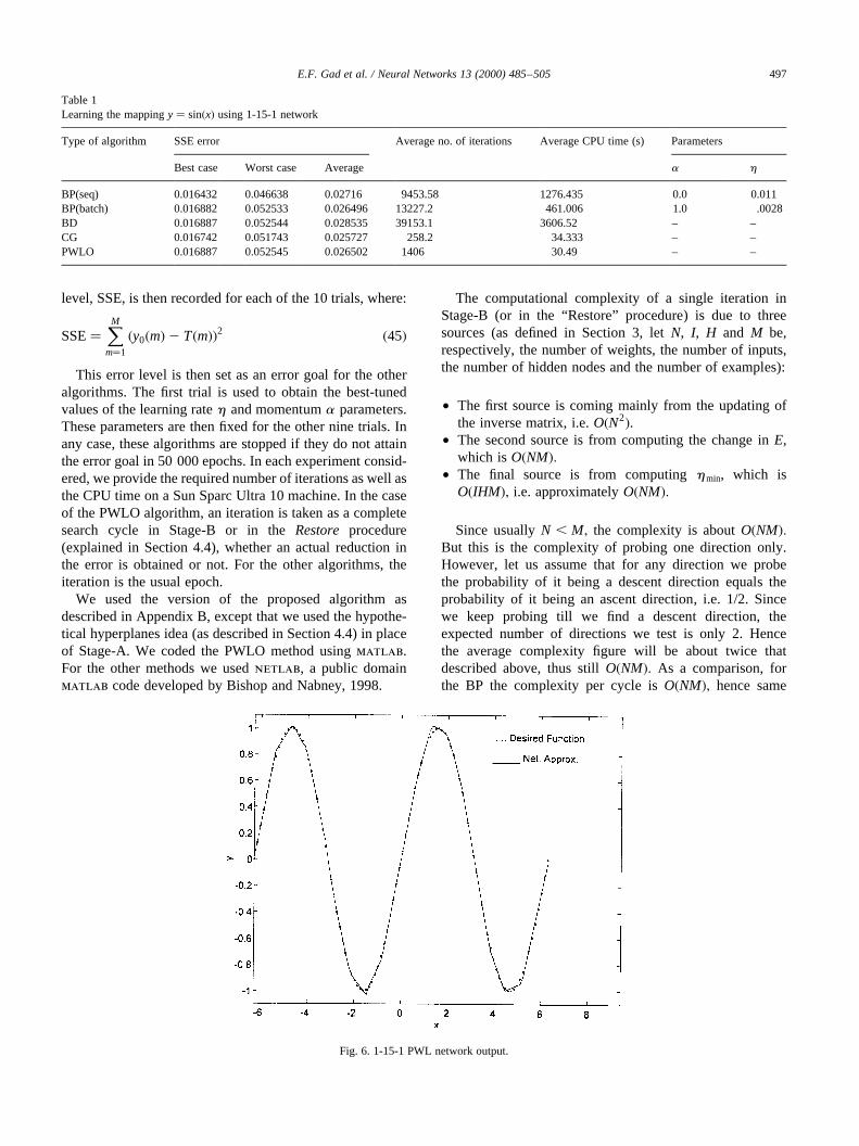
level, SSE, is then recorded for each of the 10 trials, where:

SSE�XMm�1

�y0�m�2 T�m��2 �45�

This error level is then set as an error goal for the otheralgorithms. The first trial is used to obtain the best-tunedvalues of the learning rateh and momentuma parameters.These parameters are then fixed for the other nine trials. Inany case, these algorithms are stopped if they do not attainthe error goal in 50 000 epochs. In each experiment consid-ered, we provide the required number of iterations as well asthe CPU time on a Sun Sparc Ultra 10 machine. In the caseof the PWLO algorithm, an iteration is taken as a completesearch cycle in Stage-B or in theRestore procedure(explained in Section 4.4), whether an actual reduction inthe error is obtained or not. For the other algorithms, theiteration is the usual epoch.

We used the version of the proposed algorithm asdescribed in Appendix B, except that we used the hypothe-tical hyperplanes idea (as described in Section 4.4) in placeof Stage-A. We coded the PWLO method usingmatlab.For the other methods we usednetlab, a public domainmatlab code developed by Bishop and Nabney, 1998.

The computational complexity of a single iteration inStage-B (or in the “Restore” procedure) is due to threesources (as defined in Section 3, letN, I, H and M be,respectively, the number of weights, the number of inputs,the number of hidden nodes and the number of examples):

• The first source is coming mainly from the updating ofthe inverse matrix, i.e.O�N2�.

• The second source is from computing the change inE,which isO�NM�:

• The final source is from computinghmin, which isO�IHM�; i.e. approximatelyO�NM�:

Since usuallyN , M; the complexity is aboutO�NM�:But this is the complexity of probing one direction only.However, let us assume that for any direction we probethe probability of it being a descent direction equals theprobability of it being an ascent direction, i.e. 1/2. Sincewe keep probing till we find a descent direction, theexpected number of directions we test is only 2. Hencethe average complexity figure will be about twice thatdescribed above, thus stillO�NM�: As a comparison, forthe BP the complexity per cycle isO�NM�; hence same


Table 1Learning the mappingy� sin�x� using 1-15-1 network

Type of algorithm SSE error Average no. of iterations Average CPU time (s) Parameters

Best case Worst case Average a h

BP(seq) 0.016432 0.046638 0.02716 9453.58 1276.435 0.0 0.011BP(batch) 0.016882 0.052533 0.026496 13227.2 461.006 1.0 .0028BD 0.016887 0.052544 0.028535 39153.1 3606.52 – –CG 0.016742 0.051743 0.025727 258.2 34.333 – –PWLO 0.016887 0.052545 0.026502 1406 30.49 – –

Fig. 6. 1-15-1 PWL network output.

order as our proposed method. Note also that because we areusingmatlab, some methods benefit more than others fromthe matlab speed advantage when using predominantlymatrix–vector operations. For example, the BP batch updatemethod is significantly faster than the BP sequential update(in terms of CPU time per iteration), because the gradient isevaluated using one big matrix involving all examples.

5.1. Single-dimension function approximation

Table 1 shows the results of applying the differentalgorithms to learn a network consisting of 15 hiddenneurons. The training set consists of 60 input–outputsamples drawn from the functiony� sin�x� in the

range from22p to 2p. Fig. 6 shows the PWL networkoutput after training.

5.2. Multi-dimension function approximation

The used mapping function in this example is

y� x1x2 1 x3x4 1 x5x6 1 x7x8

400�46�

wherexi is drawn at random from [0–10]. Similar mappingfunctions have been used in Barmann and Biegler-Konig(1992). Fifty examples have been used to train a networkof size 8-4-1. Table 2 shows the comparison results for an 8-4-1 network.


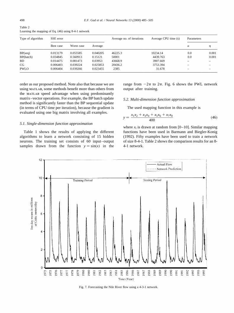
Table 2Learning the mapping of Eq. (46) using 8-4-1 network



BP(seq) 0.013179 0.055585 0.040205 46225.3 10234.14 0.0 0.001BP(batch) 0.034845 0.560913 0.15121 50001 4439.763 0.0 0.001BD 0.014475 0.081473 0.03953 43668.9 3907.669 – –CG 0.006403 0.039224 0.025853 20436.2 3753.394 – –PWLO 0.006404 0.039266 0.023455 2385 31.678 – –

Fig. 7. Forecasting the Nile River flow using a 4-3-1 network.

5.3. Time series prediction: forecasting river flow

In this experiment, the used time series consists of 650points, where each point represents the 10-day mean of theNile River flow measured at Dongola Station in northernSudan in millions of cubic meters. The data extends from1975 to 1993. These data points (used in Atiya, El-Shoura,Shaheen & El-Sherif, 1999) have been divided into two setsof 325 points each. The first set, which covers a 9-yearperiod (1975–1984) has been used as a training set for anetwork consisting of three hidden neurons. An input exam-ple consists of three previous measurements and an addi-tional measurement for the same period in the precedingyear. The second set has been used to test the networkprediction as shown in Fig. 7. Table 3 displays a summaryof the 10 trials. Fig. 8 presents a graphical comparisonbetween the learning speed of the BD and the PWLO algo-rithms. From Fig. 8, it can be observed that PWLO shows atangible slow performance in the first stages of the algo-rithm in comparison to the BD. This may be referred tothe relatively large number of training examples in this

test, which resulted in stuffing the weight space with ahuge number of hyperplanes that subsequently causemany stoppages, even along very steep descent directions.However, the BD suffers too much in the vicinity of theminimum, while the PWLO encounters no substantial trou-bles to find its way to the minimum.

The average normalized root mean square error, NRMSE,of the PWLO algorithm is 0.202 for the training phase and0.231 for the testing phase, where

NRMSE��XMm�1

�y0�m�2 T�m��2=XMm�1

�T�m��2vuut �47�

For comparison, the BP(batch), BP(seq), BD and CGachieved an NRMSE of, respectively, 0.285, 0.296, 0.293and 0.194 in the training set, and an NRMSE of, respec-tively, 0.377, 0.348, 0.338 and 0.258 in the testing set. Inthis example and the other examples we have noticed thatthe training error performance, to a large extent, carried overto the generalization error performance. This means that


Table 3Results of learning to forecast the Nile River flow using a 4-3-1 network



BP(seq) 173.2549 472.3864 226.6544 50000 70349.95 0.3 0.01BP(batch) 179.5864 426.9391 230.5609 50000 2524.3 0.3 0.001BD 177.808 307.3966 214.2032 50000 2825.285 – –CG 74.17225 94.20655 82.24458 36767 7768.794PWLO 64.15788 94.23526 76.41261 4873 187.558 – –

Fig. 8. Learning speeds of BD and PWLO for the Nile River forecast problem.

whatever method beat the others in terms of training errortended to do well compared to the others in generalizationerror performance.

5.4. Binary classification problems: bankruptcy prediction

Bankruptcy prediction is a good example for binary clas-sification problems. The data set of this experiment has beenused in Odom and Sharda (1990) in their work to apply NNsin bankruptcy prediction. In this test, the inputs reflect a setof indicators defining the financial status of a given firm,while the desired output assumes a binary value to indicate apotential bankruptcy. The PWLO algorithm has beenslightly modified to binary classification problems. Thefirst modification is effected by using the binary thresholdfunction f �x� on the output of the network where:

f �x� �1 x . 0:95

x 0:05 # x $ 0:95

0 x , 0:05

8>><>>: �48�

instead of using a linear output node. The second modifica-

tion is realized by taking the SSE as the criterion to accept orreject the weight update in Stage-B or in theRestoreproce-dure instead of the least absolute deviations. The number ofexamples is 88, and we used a 5-4-1 network. Table 4summarizes the results of the 10 trials and Fig. 9 showsthe learning curves for PWLO, BD and CG.

6. Summary and conclusions

This paper has been essentially aimed at developing anovel optimization method. One advantage that this optimi-zation method offers is that it is more suitable in trainingsingle-hidden-layer digitally implemented NNs. It requiresonly the storage of anN × N matrix, whereN is the totalnumber of weights in the network. This is in contrast to theindefinite memory requirements that the BP schemes mayneed to approximate the derivatives of the sigmoidal func-tion, in addition to the potential troubles that may erupt as aresult of such an approximation.

However, the fact that this optimization method provideda radically different approach to avoid the inherent ill


Table 4Bankruptcy prediction using a 5-4-1 network



BP(seq) 0.005187 24.70495 10.89279 48152 3177.248 0.3 0.1BP(batch) 0.033912 29.2197 11.74011 37036 2376.906 0.5 0.005BD 0.000043 27.37903 9.6168 43888 3117.431 – –CG 1.0× 1029 3.609034 1.0413 2404 326.24 – –PWLO 0.0 3.963935 1.0797 1523 18.678 – –

Fig. 9. Learning speeds of BD, CG and PWLO for the bankruptcy prediction problem.

conditioning associated with the gradient optimizationmethod used by the BP algorithms is by far another moreimportant advantage. This can be clearly observed in theobtained results in the form of a significantly acceleratedlearning process as compared to existing techniques. Wecould see, for example, how accurate and fast the algorithmhad been in the binary problem of the bankruptcy predictionas compared to the other algorithms.

Future research efforts could to be exerted to developefficient heuristics to avoid unnecessary stoppages alongvery steep descent directions. For example, one can use ahybrid technique by starting with BP training in the firststages and switching to the PWLO algorithm when the BPbecomes very slow. Another issue that we plan to consideris to improve the performance for very large sets of trainingdata (thousands or tens of thousands of examples). For sucha case the number of hyperplane boundaries increasessignificantly, and the algorithm loses part of its advantageover the other algorithms. The global optimization is alsoanother candidate issue that needs to be tackled.

Acknowledgements

A.A. would like to acknowledge the support of NSF’sEngineering Research Center at Caltech. The authorswould like to thank Prof. M. Odom for supplying the bank-ruptcy data.

Appendix A. Recursive matrix inversion

Suppose we have a nonsingular matrixA [ RN×Nandsuppose thatA21 is already known. We now wish tocomputeA21

b , whereAb is obtained fromA by exchangingtherth row with a vectorb [ R1×N

: Firstly, let us writeb asa linear combination of the rows ofA:

b �XNi�1

yiai ; yi [ R �A1�

in matrix form

y � �AT�21bT � �A21�TbT �A2�from Eq. (A1) we have

ar � 1yr

b 2XNi�1i±r

yi

yrai

or in matrix form

ar � hT�Ab� �A3�where,

hT � 2y1

yr;…;2

yr21

yr;

1yr

; 2yr21

yr;…;2

yN

yr

� ��A4�

Using Eq. (A3), we can write

A � EAb �A5�

where the matrixE [ RN×Nis obtained from the identitymatrix by exchanging therth row with hT

: MultiplyingEq. (A5) byA21 andA21

b from both sides we get

A21b � A21E �A6�

By inspecting Eq. (A3), we can deduce the necessary condi-tion for the existence ofA21

b ; i.e.yr ± 0: Thus to inspect thesingularity condition ofAb, we can obtainyr by multiplyingthe rth row of �A21�T (or the rth column ofA21) by thevectorb.

procedure Recursive_Inverse_by_Row_Exchange(C, b, r)commentGiven the inverseC of some matrix, sayA, this algorithmcomputes the inverse of the matrixAb, where Ab isobtained fromA by replacing therth row, ar , with therow vector b. The procedure uses the matrixD as atemporary storage forA21

b : Note that this algorithmpresumes that the new matrixAb will be nonsingular.Hence, the calling procedure has to check the existenceof A21

b :

beginDefine the matrixD [ RN×N

y � CbT

hT � 2y1

yr;…;2

yr21

yr;

1yr

; 2yr21

yr;…;2

yN

yr

� �

for i � 1 to N {for j � 1 to N {

if j � r thendij � hjcir

elsedij � hjcir 1 cij

}}return (D)

end

Appendix B. Pseudo code procedure

Procedure Initializationcommentak is thekth row of the matrixA;ck is thekth column of the matrixC � A21;

The indicesm, j, i are understood to scan the ranges�m�1;…;M�; �j � 1;…;H� and�i � 0;1;…; I � wherever theyappear.


begin(1) Start by assigning random values to wji ; vj :

(2) Determine the members of the sets S2m; SL

m; andS1m:

Use Eqs. (9)–(11)(3) Compute w0ji � wji ·vj

(4) Define the vectors: w 0jT U �w0jo;w0j1;…;w0jI �; xTU

�w01o;…;w01I ;w02o;…;w02I ;… …;w0Ho;…;

w0HI ; vo; v1;…; vH�(5) Define the vectorsaIa

j;m andaIbj;m Use Eqs. (35) and

(36)(6) Define the constantsbIa

j;m � bIbj;m � 0; bII

m � 2T�m�(7) Define the hyperplanes HIaj;m U { kaIa

j;m; xl 1 bIaj;m �

0; HIbj;m U { kaIb

j;m; xl 1 bIbj;m � 0}

(8) Initialize the set �H to the empty setf(9) Define the matrixA [ RN×N and the vectorb [ RN

(10) let k� 1(11) Call-Procedure Stage_A

end

ProcedureStage-Abeginwhile k # N

begin(1) compute yo�m�, e�m� : Use Eqs. (8) and (33)(2) Define the vectorsaII

m: Use Eq. (37)(3) Define the hyperplanes HIIm : HII

m U { kaIIm; xl 1

bIIm � 0}

(4) Compute the gradient vectorg(5) Compute the search directionh

if k � 1 thenh � 2g

elseUse Eq. (24)

(6) Compute the values ofhIaj;m; h

Ibj;m andhII

m : UseEqs. (28), (29) and (32)(7) Determine the indices�jp1;mp

1�; �jp2;mp2�; mp such

that:

hIajp1;m

p1� min

j;m{hIa

j;muhIaj;m . 0} ;

hIbjp2;m

p2� min

j;m{hIb

j;muhIbj;m . 0} ;

hIImp � min

m{hII

muhIIm . 0}

(8) Compute the minimum step sizehmin; hmin �min�hIa

jp1;mp1;hIb

jp2;mp2;hII

mp �(9) Denote the nearest hyperplane asHk �{ ka ; xl 1 b � 0} ; then insert it as the kth memberin �H:

(10) Update the matrix A and the vector bcorrespondingly.

ak � a ; bk � 2b ; �H � �H < { Hk}

(11) Update the weights

w0ji � w0ji 1 hminhj�I11�2I1i ;

vj � vj 1 hminhH�I11�111j ; x � x 1 hmin·h

;(12) Compute wji : wji � w0ji =vj

(13)Compute the sets S2m; SL

m; andS1m: Use Eqs. (9)–

(11)

(14) Increment k� k 1 1end(15) Call-Procedure Stage_B

end

ProcedureStage-BbeginSet: SINGULAR_Flag � FALSE

LOCAL_MIN_Flag � FALSELOCAL_MIN_Ind � 0

y � 0:5; C � A 21; [� 10E 2 6;

Compute the error E using Eq. (14).while E . Emin and LOCAL_MIN_Flag � FALSE

begin(1) compute yo�m�, e�m� : Use Eqs. (8) and (33)(2) Define the vectorsaII

m: Use Eq. (37)(3) Define the hyperplanes HIIm asHII

m U { kaIIm; xl 1

bIIm � 0}

(4) Create a new search direction

by � b 1 y ek; xy � C·by;

h � �xy 2 x�=ixy 2 xi

(5) Repeat steps (6) through (9) of Stage_A to findand identify the nearest hyperplane.(6) Will matrix A become singular if the vectorabecomes its kth row? Test for singularity using themethod developed in Appendix A.

if uka ; cklu ,[ thenSINGULAR_Flag � TRUE

elseSINGULAR_Flag � FALSE

w0ji ;new� w0ji 1 hminhj�I11�2I1i ;

vj;new� vj 1 hminhH�I11�111j ;

xnew� x 1 hminh

(7) Compute the new value of the error function:Enew� E�w0ji ;new; vj;new�

if Enew . E or SINGULAR_Flag � TRUE then


{k � k 1 1if �k . N� then {

k � 1;y � 2y;

}LOCAL_MIN_Ind � LOCAL_MIN_Ind 1 1if LOCAL_MIN_Ind � 2N then

LOCAL_MIN_Flag � TRUE}else

begin(8) An accepted step. Update as in Step (10)and (11) of Stage_A.(9) Update the matrix C�Recursive_Inverse_by_Row_Exchange�C; ak; k�(10)Remove the kth member of the set�H andinsert the nearest hyperplane as the newmember.(11) Store the previous configuration of thesets S2m; SL

m; andS1m

S2m � S2

m; SLm � SL

m; S1m � S1

m

(12) Compute wji : wji � w0ji =vj :

(13) Compute the new configuration of thesets S2m; SL

m andS1m

(14) Detect the emergence of any corruptedtype II hyperplanes in�H

T U { p [ {1 ;2;…M} uHIIp , �H}

V U { p [ TuS2p ± S2

p or SLp ± SL

p or S1p ± S1

p

(15) If there are any corrupted type II hyper-planes then call Restore procedure:

if V ± f then {

G � { r [ {1 ; 2;…;N} uar � aIIp for all p [ V}

Call-Procedure Restore(G )}

(16) Reset the local Minimum Indicator tozero: LOCAL_MIN_Ind � 0

end/* end ofif –elsestatement*/end/* end ofwhile statement*/end/* end of the Stage-Bprocedure*/

ProcedureRestore(G )beginSINGULAR_Flag � FALSEfor r � 1 to uG u

begin(1) Let k� G�r�then Repeat steps (1) through (6) of

Stage_A(2) Computeh1

min, the minimum step size required toreach the nearest hyperplane along the “positive”direction ofh:

(a) find the indices�jp1;mp1�; �jp2;mp

2�; mp such that

hIajp1;m

p1� min

j;m{hIa

j;muhIaj;m . 0} ;

hIbjp2;m

p2� min

j;m{hIb

j;muhIbj;m . 0} ;

hIImp � min

m{hII

muhIIm . 0}

(b) h1min� min�hIa

jp1;mp1;hIb

jp2;mp2;hII

mp�(3) Computeh2

min, the minimum step size required toreach the nearest hyperplane along the “negative”direction ofh:

(a) find �jp1;mp1�; �jp2;mp

2�; mp such that

hIajp1;m

p1� max

j;m{hIa

j;muhIaj;m , 0} ;

hIbjp2;m

p2� max

j;m{hIb

j;muhIbj;m , 0} ;

hIImp � max

m{hII

muhIIm , 0

(b) h2min� max�hIa

jp1;mp1;hIb

jp2;mp2;hII

mp�

(4) Select the accepted step size{h1min or h2

min} asthe one that would further reduce E; denote it byhmin:

(5) Denote the hyperplane associated withhmin asHk � {

a ; x

�1 b � 0}

(6) Repeat steps (6) and (7) of Stage_B to test for thesingularity of the matrixA if a becomes the kth rowand to compute Enew; respectively.if SINGULAR_Flag � FALSE then

(7) Repeat steps (8) through (10) of Stage_B. toupdate.

endend

Appendix C. The error is nonincreasing along thetrajectories

For Procedure 1 it is clear since in Step B we take a steponly if the new error is less than the old error.

For Procedure 2, we take a step ifgThi , 0: Since in thequadrant (region) the considered the error function is linear,the new error is given by

E�xnew� � E�xold�1 gT�xnew 2 xold� � E�xold�1 hgThi

, E�xold�since as mentionedgThi , 0:


Appendix D. Local minimum for piecewise-linearfunctions

Assume we are at an intersection ofN hyperplanes, atpoint x0; given by

Ax0 � b �D1�(see Eq. (38)). Assume that we have explored the 2N direc-tions:

hi � A21i b�i� 2 x0 �D2�

where

b�i� � �b1;…; �bi 1 y�;…;bN�T

for i � 1;…;N and

b�i� � �b1;…; �bi2N 2 y�;…;bN�T

for i � N 1 1;…;2N: The indexi in A i reflects the fact thatin the different regions aroundx0, theaII rows of A mighthave changed, as discussed in Section 4.3. Using Eqs. (D1)and (D2), we can write

hi � yA 21i ei i � 1;…;N

hi � 2yA 21i ei2N i � N 1 1;…;2N

�D3�

Let x 0 be a point in the neighbourhood ofx0. Let us expressx 0 2 x0 as a linear combination ofN of the hi’s:

x 0 � x0 1XNj�1

ljhij �D4�

under the condition thathi and hi1N cannot be togetherrepresented in the expansion. Such an expansion is possible,sinceA i is nonsingular, and hence any choice ofN hi j will belinearly independent (because of relation (D3)).

Next we show that there is a set ofN hi j ’s such thatexpansion (D4) results in nonnegativelj : Let us arrangethe hi j ’s as columns in a matrixH, and let us arrange thelj ’s as a column vectorl. Then

x 0 2 x0 � Hl: �D5�From Eq. (D3) we get

H � yA 21E �D6�whereE is a diagonal matrix withejj � 11 or 21 depend-ing on the choice ofhij ; and A is the constraint matrixassociated with the region flanked by thehi j vectors.Then, from Eqs. (D5) and (D6), we get

l � 1y

EA�x 0 2 x0� �D7�

where we used the fact thatE21 � E:. We will show herethat if l has negative components, then it is possible tochange the basis vector combination, in order to achievenonnegativelj : Consider thelj ’s corresponding to type Iconstraints. They will be equal to�1=y�ejja

Ikj�x 0 2 x0�: If

they are negative, then replace the corresponding basisvector hi j by 2h 0i j ; and this will change the sign ofejj ;

hence the newlj will be positive. After changing thebasis vectors associated with type I constraints, the rowsof the A matrix associated with type II constraints willhave changed, creating a new matrixA 0 and a new vectorl 0: Then we observe thel 0j ’s associated with type IIconstraints. If they are negative, then again we replace thecorresponding basis vectorhi j by 2h 0i j : This replacementwill not tamper further with theA matrix, and hence thisnew basis results in nonnegativelj :

Since in the region spanned by anyN basis vectorshij ; theerror function is linear (no discontinuities), then by usingEq. (D4) we get

E�x 0� � E�x0�1XNj�1

ljE�hi j � �D8�

Using Eq. (D2) and the theorem assumption that all the 2Ndirections lead to a higher error we haveE�hi j � . 0; andhenceE�x 0� . E�x0�:

Appendix E. Convergence in a finite number ofiterations

The number of points that could possibly be visited isfinite, and equals the number of intersections ofN hyper-plane boundaries (or more thanN in case of degeneracies).Along a descent trajectory no point is visited more thanonce. This is also true along the trajectories of constantE,because of the mechanism described to prevent cycling.Also, no move will carry us to infinity. If the move is adescent move, then an infinite-sized move will result inEgoing to minus infinity, which is impossible becauseEcannot be negative. If the move is a constant-E move,then if we encounter a move that will go to infinity, thenwe can simply ignore this move and choose another searchdirection.

To summarize, there is a finite number of points, everypoint is visited at most once, and every move leads fromonepoint to another(unless we are at a local minimum). Hencethe number of iterations is finite.

References

Abu-Mostafa, Y. (1989). The Vapnik-Chernovenkis dimension: informa-tion versus complexity in learning.Neural Computation, 1, 312–317.

Atiya, A., El-Shoura, S., Shaheen, S., & El-Sherif, M. (1999). A compar-ison between neural network forecasting techniques: case study: riverflow forecasting.IEEE Transactions on Neural Networks, 10 (2), 402–409.

Barmann, F., & Biegler-Konig, F. (1992). On a class of efficient learningalgorithms for neural networks.Neural Networks, 2, 75–90.

Batruni, R. (1991). A multilayer neural network with piecewise-linearstructure and backpropagation learning.IEEE Transactions on NeuralNetworks, 2, 395–403.


Battiti, R. (1992). 1st order and 2nd order methods for learning betweensteepest descent and Newton method.Neural Computation, 4, 141–166.

Battiti, R., & Tecchiolli, G. (1994). Learning with first second and noderivatives: a case study in high energy physics.Neurocomputing, 6,181–206.

Baum, E., & Haussler, D. (1989). What net size gives valid generalization?Neural Computation, 1, 151–160.

Benchekroun, B., & Falk, J. (1991). A nonconvex piecewise-linear optimi-zation problem.Computers in Mathematical Applications, 21, 77–85.

Bishop, C. (1995).Neural network for pattern recognition. Oxford: OxfordUniversity Press.

Bishop, C., Nabney, I. (1998).netlab. Neural Network Simulator, http://www.ncrg.aston.ac.uk/netlab/index.html.

Bobrowski, L. (1991). Design of piecewise linear classifiers from formalneurons by a basis exchange technique.Pattern Recognition, 24, 863–870.

Bobrowski, L., & Niemiro, W. (1984). A method of synthesis of lineardiscriminant functions in the case of nonseparability.Pattern Recogni-tion, 17, 205–210.

Golden, R. (1996).Mathematical methods for neural network analysis anddesign. Cambridge, MA: MIT Press.

Hammerstrom, D. (1992). Electronic neural network implementation,Tutorial. International Joint Conference on Neural Networks.Balti-more, MD.

Haykin, S. (1994). VLSI implementation of neural networks.Neuralnetworks: a comprehensive foundation. New York: IEEE Press (chap.15).

Hush, D., & Horne, B. (1998). Efficient algorithms for function approxima-tion with piecewise linear sigmoidal networks.IEEE Transactions onNeural Networks, 9 (6), 1129–1141.

Kevenaar, T., & Leenaerts, D. M. W. (1992). A comparison of piecewise-linear model descriptions.IEEE Transactions on Circuits and Systems,39, 996–1004.

Lin, J.-N., & Unbehauen, R. (1990). Adaptive nonlinear digital filter withcanonical piecewise-linear structure.IEEE Transactions on on CircuitSystems, 37, 347–353.

Lin, J.-N., & Unbehauen, R. (1995). Canonical piecewise-linear neuralnetworks.IEEE Transactions on Neural Networks, 6, 43–50.

Michel, A., Si, J., & Yen, G. (1991). Analysis and synthesis of a class ofdiscrete-time neural networks described in hypercubes.IEEE Transac-tions on Neural Networks, 2 (1), 32–46.

Moody, J. (1992). The Effective number of parameters: an analysis ofgeneralization and regularization in nonlinear learning system. In J.Moody, S. Hansen & R. Lippmann (Eds.),Advances in Neural Informa-tion Processing Systems(pp. 847–854), 1992,4.

Odom, M., & Sharda, R. (1990). A neural network model for bankruptcyprediction. InProceedings of the IEEE International Conference onNeural Networks(pp. 163–168).

Pao, Y. H. (1989).Adaptive pattern recognition and neural networks. Read-ing, MA: Addison-Wesley.

Saarinen, S., Bramely, R., & Cybenko, G. (1993). Ill-conditioning in neuralnetwork training problems.SIAM Journal of Scientific Computing, 14(3), 693–714.

Staley, M. (1995). Learning with piecewise-linear neural networks.Inter-national Journal of Neural Systems, 6, 43–59.

Vogl, T., Mangis, J., Rigler, A., Zink, W., & Alkon, D. (1988). Acceleratingthe convergence of the back-propagation method.Biological Cyber-netics, 59, 257–263.


a new algorithm for learning in piecewise-linear neural ...alumnus.caltech.edu/~amir/pwl.pdf ·...

Documents