A NEW ANT COLONY OPTIMIZATION APPROACH FOR THE

SINGLE MACHINE TOTAL WEIGHTED TARDINESS SCHEDULING

PROBLEM

Davide Anghinolfi, Massimo Paolucci

Department of Communication, Computer and System Sciences

University of Genova

Via Opera Pia 13

16145 Genova, Italy

{anghinolfi, paolucci}@dist.unige.it

Fax: +39-010-3532948, Phone: +39-010-3532996

Abstract

In this paper the NP-hard single machine total weighted tardiness scheduling problem in presence of sequence-

dependent setup times is faced with a new Ant Colony Optimization (ACO) approach. The proposed ACO

algorithm is based on a new global pheromone update mechanism, which makes the pheromone trails

asymptotically range between two bounds arbitrarily fixed and the ACO learning mechanism independent of the

values of the objective function of the considered problem. Other features of the algorithm include a

diversification mechanism for the solution construction phase based on a local pheromone update rule whose

effects are restricted to the single iterations, and a cumulative option for the global pheromone update rule. An

experimental campaign, carried out on a benchmark available from the literature, was executed to evaluate the

proposed ACO and the effectiveness of its optional features. In particular, the obtained results were compared

with the ones of a recently proposed ACO algorithm for the same problem by Liao and Juan (2005). The analysis

of the outcomes showed the competitiveness of the new ACO approach, which was able to improve about 72%

of the best known results for the benchmark. Finally, a further investigation on a different benchmark set of

instances without setup times showed the robustness of the proposed ACO algorithm.

Keywords: Ant Colony Optimization, Metaheuristics, Scheduling, Total Weighted Tardiness.

1. Introduction

Ant Colony Optimization (ACO) is a recent metaheuristic approach which aims at exploiting the successful

behaviour of real ants in cooperating to find shortest paths to food for solving combinatorial problems (Dorigo

and Stützle, 2002), (Dorigo and Blum, 2005). In most of the real species ants have an effective indirect way to

communicate each other which is the most promising trail, and finally the optimal one, towards food: ants

produce a natural essence, called pheromone, which they leave on the followed path to food in order to mark it.

The pheromone trail evaporates over time and it disappears on the paths abandoned by the ants. On the other

hand, the pheromone trail can be reinforced by the passage of further ants: thus, effective (i.e., shortest) paths

leading to food are finally characterized by a strong pheromone trail, and they are followed by most of ants. The

ACO metaheuristic was first introduced by Dorigo, Maniezzo and Colorni (1991, 1996) and Dorigo (1992), and

since then it has been the subject of both theoretical studies and applications. ACO combines both Reinforcement

Learning (RL) (Sutton and Barto, 1998) and Swarm Intelligence (SI) (Kennedy and Eberhart, 2001) concepts:

each single agent (an ant) takes decisions and receives a reward from the environment, so that the agent’s

policy aims at maximizing the cumulative reward received (RL);

the agents exchange information to share experiences and the performance of the overall system (the ant

colony) emerges from the collection of the simple agents’ interactions and actions (SI).

ACO metaheuristic has been successfully applied to several combinatorial optimization problems, from the

first travelling salesman problem applications (Dorigo, Maniezzo and Colorni, 1991 and 1996), to vehicle

routing problems (Bullnheimer, Hartl and Strauss, 1999), (Reinmann, Doerner and Hartl, 2004), and to single

machine and flow shop scheduling problems (den Besten, Stützle and Dorigo, 2000), (Gagné, Price and Gravel,

2002), (Ying and Liao, 2004).

This paper proposes a new Ant Colony Optimization (ACO) approach to face one among the most

important scheduling problems, i.e., the single machine total weighted tardiness scheduling with sequence-

dependent setup times (STWTSDS) problem. The choice of the STWTSDS problem as reference application for

the proposed ACO approach is motivated by the relevance of the considered problem for manufacturing

industries. The importance of performance criteria involving due dates, such as (weighted) total tardiness or total

earliness and tardiness (E-T), as well as the explicit consideration of sequence-dependent setups, has been widely

recognized in many real industrial contexts. Both in the survey on US manufacturing practise by Wisner and

Siferd (1995) and in the one by Panwalkar, Dudek and Smith (1973) meeting the due dates is identified as the

most important scheduling objective. Criteria weighting both the early and the tardy completion of jobs with

respect to their due dates, the so-called non-regular objectives (Baker and Scudder, 1990), have been considered

to encompass the just-in-time (JIT) philosophy aiming at reducing the level of inventories. Among the regular

objectives based on due dates, the minimization of the total weighted tardiness is the subject of a very large

amount of literature on scheduling; however, the coverage of the problem including an explicit consideration of

sequence-dependent setups is not so extended. Setup operations are necessary to prepare production resources

(e.g., machines) for the job to be executed next, and whenever they depend on the (type of) preceding job just

completed they are called sequence-dependent setups. In the survey by Panwalkar, Dudek and Smith (1973) the

presence of sequence-dependent setups has been observed in a relevant number of industrial scheduling contexts.

Nevertheless, it is often assumed the setup times independent of the sequence of jobs on the machine, including

them into processing times; alternatively, setup times are simply disregarded and eventually inserted in the so

found solutions. In a review on machine scheduling problems involving setups, Allahverdi, Gupta, and

Aldowaisan (1999) provided a number of industrial examples including sequence-dependent setups and they

indicated the importance of taking into account setup times separately from job processing times. In addition, it

was underlined in Rubin and Ragatz (1995) how the difficulty of total tardiness scheduling on a single machine

is increased by the presence of sequence-dependent setups, since dominance conditions used for simple tardiness

problems do not hold true. In addition, although in general weighted tardiness problems with sequence-

dependent setups may originate from single or multi-machine contexts, it was observed that the solution of single

machine problems is often required even in more complex environments (Pinedo, 1995).

The work presented in this paper aims at analysing the behaviour of an ACO approach which mainly differs

from previous ones in the literature for a new pheromone trail model based on an original global pheromone

update (GPU) rule. In particular, (a) pheromone values are independent of the problem cost (or quality) function

and they are bounded within an arbitrarily chosen and fixed interval; (b) the new GPU rule implements the ant

colony learning system by exploiting the solution quality as a sort of signal driving the reward mechanism, and

updating the pheromone values accordingly; in addition, this GPU rule makes the pheromone values

asymptotically increase (decrease) towards the upper (lower) bound without requiring any explicit cut-off,

differently from the Max-Min Ant System (MMAS) (Stützle and Hoos, 2000), where upper and lower bounds for

pheromone values are used as well; finally, (c) a diversification strategy is adopted which is based on a

temporary perturbation of the pheromone values performed by a local pheromone update (LPU) rule within any

single iteration.

The rest of the paper is organized as follows: Section 2 introduces a formal definition of the STWTSDS

problem and reviews the relevant literature for this problem and for previous related ACO approaches. Section 3

illustrates the basic aspects of the ACO approach, discussing how it can be applied to the STWTSDS problem

and highlighting the new features introduced. Section 4 shows the extended experimental campaign performed

on the benchmark set generated by Cicirello (2003), whose best known results have been very recently updated

both in Cicirello (2006) and in Lin and Ying (2006), and it compares the proposed ACO with the one presented

in Liao and Juan (2005); in addition, the results obtained to test the robustness of the proposed ACO on a single

machine total weighted tardiness scheduling problem benchmark available from ORLIB are presented. Finally,

Section 5 draws some conclusions.

2. Problem definition and literature review

Formally, the STWTSDS problem requires the scheduling of a set of n independent jobs, which are all ready for

processing at time zero, on a single machine which is continuously available and can process only one job at a

time. For each job j=1,..., n, the following quantities are given: a processing time pj, a due date dj and a weight

wj. A sequence-dependent setup time sij should be waited before starting the processing of job j immediately

sequenced after job i. The job tardiness is defined as Tj=max(0, Cj-dj), being Cj the completion time of job j, and

the job is said tardy if Tj>0. A schedule corresponds to a feasible sequencing of the jobs on the machine: due to

the regularity of the problem objective (Baker and Scudder, 1990), having fixed a feasible sequencing, each job

must complete at its earliest completion time. The scheduling objective is the minimization of the total weighted

tardiness, i.e.,

∑==

n

jjjTwZ

1min (1)

This problem, which is denoted as 1/sij/ΣwjTj , is strongly NP-hard since it is a special case of the 1//ΣwjTj

that has been proved to be strongly NP-hard by Lawler (1997); the complexity of the considered problem,

confirmed by the fact that the special case without setups and with unitary weights is still NP-hard (Du and

Leung, 1990), justifies the research of heuristic approaches for its solution in practical cases. Nevertheless, exact

algorithms based on branch and bound (B&B) or dynamic programming approaches have been proposed, but

they are able to tackle instances of reduced dimensions. For example, an early B&B algorithm for the

STWTSDS problem was proposed in Rinnooy Kan, Lageweg and Lenstra (1975); Abdul-Razaq, Potts and van

Wassenhove (1990) faced the single machine total tardiness scheduling with sequence-dependent setups

(STTSDS) problem, whereas the algorithm in Potts and van Wassenhove (1985) was able to solve up to 40-job

instances for the sequence-independent problem; Luo and Chu (2006) recently devised a B&B algorithm for the

STTSDS solving up to 30-job instances with reduced computational times. Most of the recent research on total

tardiness scheduling with sequence-dependent setups is focused on the development of heuristics: in particular,

constructive heuristics, generally corresponding to dispatching rules, improvement heuristics and metaheuristics.

The well-known apparent tardiness cost with setups (ATCS) heuristic, proposed by Lee, Bhaskaran and Pinedo

(1997), appears to be the best constructive approach for the STWTSDS problem; such heuristic extends to the

case of sequence-dependent setups the time-dependent apparent tardiness cost (ATC) rule defined a decade

before by Vepsalainen and Morton (1987). Constructive heuristics usually require a small computational effort

(for this reason they may be preferred in industrial applications), but they are outperformed by improvement

approaches, as well as metaheuristics, which, in turn, are usually much more computational time demanding.

Improvement approaches consist of local search algorithms that, starting from an initial solution produced by a

simple constructive rule, explore a succession of neighbouring solutions until no further improvement is

possible. As noted in the paper by Cicirello and Smith (2005), which includes a survey of heuristic approaches

for the STWTSDS problem, also Lee, Bhaskaran and Pinedo, (1997) proposed a local search procedure based on

a reduced set of swap and insert moves to improve the solution generated by the ATCS rule. The dominance of

improvement approaches over constructive ones is witnessed, for example, in Potts and van Wassenhove (1991),

where the effectiveness of simple pair-wise interchange methods against dispatching rules for the single machine

total weighted tardiness problem was shown; more recently, constructive heuristics were compared to a memetic

algorithm in França, Mendes and Moscato (2001), or also in Anghinolfi and Paolucci (2006), where a hybrid

metaheuristic was proposed for a similar parallel machine case. Cicirello and Smith (2005) analysed the

behaviour of several stochastic search procedures for the STWTSDS, showing the effectiveness of introducing

randomization. In particular, the authors developed several algorithms, a value-biased stochastic sampling

(VBSS), a VBSS with hill-climbing (VBSS-HC) and a simulated annealing (SA), that were compared to limited

discrepancy search (LDS) and heuristic-biased stochastic sampling (HBSS) for a 120 benchmark problem

instances defined by Cicirello (2003) and available on the web. Several metaheuristic approaches have been

proposed for the STTSDS problem: genetic algorithms (GA) in Rubin and Ragatz (1995) and in Armentano and

Mazzini (2000); a memetic algorithm combining GA with local search in França, Mendes and Moscato (2001); a

SA approach (Tan and Narasimhan, 1997); a greedy randomized adaptive search procedure (GRASP) in Feo,

Sarathy and McGahan (1996). Tan et al. (2000) compared four implementations of B&B, GA, random-start pair-

wise interchange (RSPWI) and SA proposed for the STTSDS in previous works by the same authors, concluding

that SA and RSPWI are suitable approaches to face larger instances, whereas the GA shows the worst

performance. In recent times, the Cicirello’s best known results were independently improved in Lin and Ying

(2006) and in Cicirello (2006). Lin and Ying (2006) developed three approaches for the STWTSDS, i.e., a SA, a

GA and a tabu search (TS), whose best results over 10 runs were compared against the Cicirello’s (2005) best

known ones; the results reported by the authors show that all the three algorithms were able to improve the

previous best known results for more than 71% of the instances with an average computation time for each

single run of 27s. Cicirello (2006) presented a GA approach for the STWTSDS problem based on a new non-

wrapping order crossover (NWOX) operator, derived from the well-known order crossover (OX) operator,

whose purpose is to propagate to the offspring not only the jobs’ order but also their absolute positions in the

sequences; this new NWOX operator appeared well-suited for the STWTSDS problem, and the GA presented in

Cicirello (2006) was able to improve 49 of the 120 best known results of the Cicirello’s (2003) benchmark.

In recent years, several ACO approaches have been proposed to face total tardiness scheduling problems

which may include or not sequence-dependent setups. A first implementation was studied in Bauer et al. (1999),

where the authors adapted the Ant Colony System (ACS) (Dorigo and Gambardella, 1997) to the single machine

total tardiness problem, showing that their algorithm outperforms a set of leading heuristics for this problem. An

analysis of the combination of different local search strategies with an ACS algorithm for the total weighted

tardiness problem was proposed by den Besten, Stützle and Dorigo (2000), who highlighted as dominant strategy

the use of solution neighbourhoods based on the concatenation of simple moves; the ACO algorithm in den

Besten, Stützle and Dorigo (2000) tested over the ORLIB benchmark (www.ms.ic.ac.uk/info.html) found always

the best known solution even for the largest instances (100 jobs) with 6.99s as average CPU time. Merkle and

Middendorf (2000, 2003) defined a new approach of evaluating pheromone values, called Pheromone

Summation (PS) rule, in an ACO algorithm that extends to total weighted tardiness scheduling problems the ACS

proposed for traveling salesman problem (TSP) in Dorigo and Gambardella (1997). Since for standard ACO

approaches the probability p(h, j) of a job j of being scheduled in a sequence place h depends on single

pheromone value associated with the pair (j, h), the aim of the PS rule is to avoid a too much delayed scheduling

of jobs which fail to be sequenced in their most favourite place. Similarly, Merkle and Middendorf (2001)

pointed out that for permutation scheduling problems the sequential solution construction procedure usually

adopted in ACO algorithms can be based on a probability p(h, j) that should take into account the previous

decisions for the places preceding h; hence the authors devised an ACO approach which alternates iterations

where “random” ants consider the sequence places in random order to iterations where “sequential” ants assign

the jobs in the sequence order but including also a suitable heuristic information in the selection probability. In

Merkle and Middendorf (2002) it was remarked the need of methods like the PS rule for permutation problems

where good solutions show a so-called “similarity property”, i.e., they usually differ for a small number of

places; in alternative to the PS rule the authors defined a new Relative Pheromone Evaluation (RPE) method,

based on a normalization of pheromone values, that for a single machine total earliness with multiple due dates

scheduling problem outperformed both standard and PS rule pheromone evaluation approaches. Gagné, Price

and Gravel (2002) showed the effectiveness of an ACO algorithm for the STTSDS problem which includes a

lookahead information, obtained from a lower bound described in Tan et al. (2000), in the heuristic component

of the transition rule used to select the next job to be included in a partial schedule. Quite recently, the ACO

algorithm by Gagné, Price, and Gravel (2002), together with B&B and other metaheuristic approaches, has been

outperformed by different variants of GRASP for the STTSDS proposed by Armentano and Bassi de Araujo

(2006) and by Gupta and Smith (2006). An ACO algorithm for the STWTSDS has been proposed in Liao and

Juan (2005), where the authors showed the appropriateness of their approach by improving about 86% of the

best results obtained with the set of improvement heuristics in Cicirello (2003) for the 120 benchmark problem

instances; also this algorithm is based on ACS, but it imposes a minimum pheromone value similarly to the

MMAS (Stützle and Hoos, 2000), and adopts a new parameter for the pheromone initialization and a different

timing for local search execution. Two final remarks may emerge from the literature review of ACO approaches

to scheduling. Firstly it can be observed that the presence of sequence-dependent setups has been mainly

considered into the heuristic information exploited by the ACO algorithms: for example, in Gajpal, Rajendran

and Ziegler (2006) sequence-dependent setups influence the heuristic used to generate a starting solution that,

after a local search enhancement, is used to initialize the pheromone trails. Secondly, the role of the local search

appears basic to improve the behaviour of ACO algorithms.

3. The proposed ACO approach

This section presents the characteristics of the new ACO approach proposed for the STWTSDS problem. For this

purpose, some notation must be introduced. In general a solution x of a single machine scheduling problem of a

set of n independent jobs is represented by a sequence σ(x)=(x[1],..., x[n]), where σ(x[h]) or simply [h],

h=1,..., n, denotes the index of the job that in solution x is sequenced in the h-th position on the machine, e.g.,

j=σ(x[h])=[h], with j=1,..., n. In addition, the position-job pairs (h, j), h, j=1,..., n, determined by a sequence σ(x)

are denoted as solution components of x.

The core of the approach proposed in this paper for ACO (denoted in the following with ACOAP) is mainly

based on the Ant Colony System (ACS) (Dorigo and Gambardella, 1997), and it includes concepts inspired to

the MMAS (Stützle and Hoos, 2000) and to the approaches in Merkle and Middendorf (2000, 2003); however,

how it will be detailed in the following, in the ACOAP algorithm such concepts are encapsulated in a new

pheromone model and exploited in a real different manner. In addition, the developed algorithm may be also

compared to the one in Liao and Juan (2005) (denoted hereinafter as ACOLJ), whose results have been taken as

main reference to evaluate the ACOAP effectiveness.

3.1 The overall ACOAP algorithm description

Figure 1 reports the very high level structure of the ACOAP algorithm.

<Figure 1 near here>

A set A of m artificial ants is considered. At each iteration k, every ant a identifies a solution kax building a

sequence )( kaxσ of the n jobs, whose objective value )( k

axZ is then simply computed by assigning to each job

its feasible (i.e., taking into account both processing times and setups) earliest start time for that sequence. Every

ant a builds the sequence )( kaxσ by iterating n selection stages: first, the set of not sequenced jobs for ant a,

0aU , is initialized as },...,1{0 nUa = ; then, at stage h=1,..., n, the ant a selects one job j from the set 1−h

aU to be

inserted in the position h of the partial sequence, and updates }{\1 jUU ha

ha

−= ; at stage h=n all the jobs are

sequenced and ∅=naU . The job selection at each stage h of the construction procedure at iteration k is based on

a rule that is influenced by the pheromone trail ),( jhkτ associated with the possible solution components (h, j),

where j∈ 1−haU .

A characteristic that distinguishes the proposed algorithm from all the previous approaches is that the

pheromone values assigned to ),( jhkτ are independent of the objective or quality function values associated

with previously explored solutions including the component (h, j). Pheromone trails here represent a sort of

measure of the utility of including a component during the construction of “good” solutions that is progressively

learned from the solution space exploration. In addition, an arbitrary range ],[ MaxMin ττ is adopted for the

pheromone values, which is independent of the specific problem or instance considered. Also in MMAS lower

and upper bounds are imposed for ),( jhkτ , but they must be appropriately selected and dynamically updated

each time a new best solution is found, taking into account the objective function values. Differently, in the

ACOAP algorithm such bounds are independent of the objective function and arbitrarily selected, since any pair

of values, such that MaxMin ττ < , can be chosen. Note that in this way Maxτ and Minτ are removed from the set

of parameters needed by the algorithm. In addition, the variation of ],[),( MaxMink jh τττ ∈ during the

exploration process, i.e., the ant colony learning mechanism, is controlled by a new GPU rule (described in the

following) that imposes a smooth variation of ),( jhkτ within these bounds such that both extremes are

asymptotically reached. Note that such a characteristic is different from MMAS, where the lower and upper

bounds are used as cut-off thresholds. The new pheromone-based learning mechanism of the ACOAP algorithm

relies on three features: (a) the new kind of asymptotic pheromone trails previously described; (b) a local

pheromone update (LPU) rule that induces a pheromone perturbation to favour a stronger intra-iteration

diversification mechanism than in standard ACS, but it keeps the scope of such perturbation restricted to each

single iteration; (c) a new unbiased global pheromone update rule. The features (b) and (c) will be detailed in the

following where, in order to make simpler and more readable the expressions, a relative pheromone value

Minkk jhjh τττ −= ),(),(' , such that ]',0[),(' Maxk jh ττ ∈ , where MinMaxMax τττ −=' , is used. The ACOAP

algorithm in Figure 1 can now be detailed.

Initialization. For each solution component (h, j), h, j=1,..., n, an initial value of the pheromone trail is assigned

by fixing 2/)(),(0 MinMaxjh τττ += ; in addition, the best current solution x* is initialized as an empty solution

and the associated objective value Z(x*) is fixed to infinity.

Job selection rule. At a selection stage h of iteration k, an ant a determines which job j∈ 1−haU is inserted in the

h-th position of the sequence as follows. First, similarly to the ACS, it is chosen which job selection rule must be

used between exploitation and exploration: a random number q is extracted from the uniform distribution U[0, 1]

and if q≤q0 the exploitation rule is used, otherwise the exploration one. The parameter q0 (fixed such that

0≤q0≤1) directs the ants’ behaviour towards either the exploration of new paths or the exploitation of the best

paths previously emerged. The exploitation rule selects the job j in a deterministic way as

[ ] }),(),('{maxarg1

kkhaUu

jhjhj βητ ⋅=−∈

(2)

whereas the exploration rule according to a selection probability ),( jhp computed as

[ ][ ]∑ ⋅

⋅=

−∈ 1),(),('

),(),('),(

haUu

kk

kk

jhjhjhjhjhp β

β

ητ

ητ (3)

The quantity ),( jhη , associated with the solution component (h, j), is an heuristic value which is computed, as

done in Liao and Juan (2005), equal to the priority ),( jhIt of assigning job j in position h at time t according to

the ATCS rule (Lee, Bhaskaran and Pinedo, 1997)

⎥⎦

⎤⎢⎣

⎡−⎥

⎦

⎤⎢⎣

⎡ −−== −

sks

pktpd

pw

jhIjh jhjj

j

jt

2

]1[

1exp

)0,max(exp),(),(η (4)

where

jhh

iiii spst ]1[

1

1][]][1[ )( −

−

=− +∑ += (5)

p and s are respectively the average processing time and the average setup time, and k1 and k2 are the

lookahead parameters fixed as originally suggested in Lee, Bhaskaran and Pinedo (1997). Therefore, similarly to

the ACO approaches previously reviewed, even in the ACOAP algorithm the influence of the sequence-dependent

setups is encapsulated in the heuristic values used in the job selection rule. The parameter βk in (2) and (3) is the

relative importance of the heuristic value with respect to the pheromone trail one at iteration k; the initial value

β0 of such parameter is updated at each iteration with the following exponential rule

kk βϕβ ⋅=+1 (6)

where ϕ is a factor fixed in [0, 1]. The progressive reduction of parameter βk was not included in previous

approaches to the STWTSDS problem, but, to the best authors’ knowledge, it has been first introduced in the

ACO algorithm proposed by Merkle, Middendorf, and Schmeck (2002) for resource constrained scheduling

problems; in this way, the influence of the heuristic values ),( jhη on the ants’ decisions diminishes iteration

after iteration, leaving to the pheromone trails the leading role of driving the solution construction process.

Finally, note that for this reason the choice of the heuristic to compute the η(h, j) values could appear less

critical, but still necessary in the initial iterations when the pheromone is equally distributed over all the possible

solution components.

Local pheromone update (intra-iteration diversification). As often done in previous ACO approaches to avoid

premature convergence of the algorithm, a LPU is performed after any single ant a completed the construction of

a solution xa in order to make more unlike the selection of the same sequence by the following ants. In the

ACOAP the local pheromone update rule adopted is

])[(;,...,1),(')1(),(' hxjnhjhjh akk στρτ ==∀⋅−= (7)

where ρ is a parameter fixed in [0, 1]. A new characteristic introduced for the ACOAP is to consider such kind of

update strictly local, i.e., to use it to favour the diversification of the sequences produced by the ants within the

same iteration. Note that rule (7) imposes a perturbation on the (relative) pheromone values which is stronger

than the one in the standard ACS approach, since it drives pheromone values towards Minτ instead of 0τ .

Therefore, here rule (7) is used to temporarily modify the pheromone values only in the single iteration scope,

since such changes are deleted before executing the global pheromone update phase and starting the next

iteration. This feature, said reset of the local pheromone update (RLPU), appears consistent with the

interpretation of the pheromone values as learned utility, as it assigns only to the GPU the crucial task of

modifying the pheromone trails according to the colony exploration experience.

Local search phase. After all the ants have completed the solution construction procedure at an iteration, an

intensification phase may be performed, which consists of one or more local search (LS) explorations starting

from a subset XLS of the solutions found in the iteration. In particular, two rules (said LS timing rules) can be

used to determine the set XLS and, depending on its cardinality, how many LS explorations must be executed:

• Best in Iteration (BI) rule: XLS always includes a single starting solution corresponding to the best solution

found in the current iteration, i.e., )(minarg,...,1

ka

makb xZx

== . Then, according to this rule a single LS is always

executed in each iteration.

• Improved Solution Without LS (ISWLS): let *WLSx be the best solution found by any ant in the previous

iterations without using the LS; then, XLS may include one or more solutions found in the current iteration k

improving *WLSx , i.e. },...,1),()(:{ * maxZxZxX WLS

ka

kaLS =<= . With the ISWLS the number of LSs

executed in one iteration can vary from zero to m, even if this latter appears a very unlikely case.

In general, any LS algorithm can be used for the intensification phase in ACOAP. In particular, an LS

algorithm similar to one in Tasgetiren, Sevkli, Liang and Gencyilmaz (2004), which in turn is based on a variant

of the variable neighbourhood search (Mladenovic and Hansen, 1997), has been adopted. The LS algorithm,

summarized in Figure 2, performs a random neighbourhood exploration allowing both an alternation of random

insert and swap moves; in addition the algorithm executes a limited number of random restarts as in the iterated

local search. Note that a similar neighbourhood structure is used in Liao and Juan (2005). Random moves consist

of picking at random two sequence positions in the current solution and inserting (swapping) the job in the first

position after (with) the job in the second one. The algorithm executes an exploration sequence first made of a

succession of random insert moves until no improvement is found, and then made of a succession of swap

moves: whenever a swap move is not able to find an improved solution, then a new sequence of random insert

moves is started and the exploration counter is incremented. After n⋅(n-1) explorations have been completed, the

algorithm executes a random restart from the current best solution. The maximum number of allowed random

restarts is bounded by n/5, thus the overall complexity of the LS algorithm is O(n3). As a result of the LS phase,

the best current solution x* is possibly updated.

<Figure 2 near here>

Global pheromone update. Two main peculiarities of the ACOAP algorithm, which differentiate it from the

previous approaches, are in the meaning given to the pheromone trail values and consequently in the way such

values are updated after the completion of an iteration. It has been already pointed out that the (relative)

pheromone values ),(' jhkτ adopted in the ACOAP range in ]',0[ Maxτ ; such values are changed in the GPU

phase with a rule, called Unbiased Pheromone Update (UPU) since it neither uses any cost nor quality function,

but it performs a smooth update of the pheromone trails associated with a set of quality solution components. Let

*kΩ be the set of the best solution components (said, the best component set) determined after the completion of

iteration k; then, the UPU rule consists of the three following steps:

1. pheromone evaporation for the solution components not included in *kΩ

*1 ),(),(')1(),(' kkk jhjhjh Ω∉∀⋅−=+ τατ (8)

where 0 ≤α ≤1 is a parameter establishing the evaporation rate;

2. computation of the maximum pheromone reinforcement ),(' jhkτΔ for the solution components in *kΩ

*),(),(''),(' kkMaxk jhjhjh Ω∈∀−=Δ τττ (9)

3. update of the pheromone trails to be used in the next iteration for the solution components in *kΩ

*1 ),(),('),('),(' kkkk jhjhjhjh Ω∈∀Δ⋅+=+ ταττ (10)

The UPU rule guarantees that ]',0[),(' Maxk jh ττ ∈ and ),(' jhkτ converges towards the bounds asymptotically

( ),(' jhkτΔ is progressively reduced as much as ),(' jhkτ approaches to Max'τ , as well as the decrease of

),(' jhkτ towards 0 in (8)) with a law similar to the most frequently used cooling schedule for the SA

metaheuristic (Kirkpatrick, Gelatt and Vecci, 1983). An example of the trend due to the UPU rule is depicted in

Figure 3. This figure shows, for a fixed solution component (h, j)=(H, J), the effect of the evaporation step (8),

with α=0.1, on the associated pheromone ),( JHkτ from its initial value τ0 at iteration k=0, to a value close to

τMin at iteration k=40; then, assuming that the component (H, J) is included in *kΩ for k=41,..., 100, the figure

shows the consequent asymptotical increase of ),( JHkτ towards τMax due to steps (9) and (10); finally,

),( JHkτ is again subject to the evaporation (8), having assumed *),( kJH Ω∉ for k>100.

<Figure 3 near here>

Two possibilities are available for defining the best component set *kΩ :

• Best-so-far (BS) solution component set: *kΩ includes only the solution components associated with x*, i.e.,

{ }])[(;,...,1:),( ** hxjnhjhk σ===Ω (11)

• Cumulative BS (CBS) solution component set: if a component (h, j) is present in x*, that is, h appeared a

“good” sequence position for job j, hence, taking into account that a tardiness cost must be minimized, it

should be sensible to consider j even more urgent for successive sequence positions if job j misses to be

sequenced as h-th; according to this rationale, the set *kΩ is defined as

{ }])[(;,...,1;,...,:),( ** hxjnhnhljlk σ====Ω (12)

An example of the effects of the UPU rule with the two different options for defining the best component set is

provided in Figure 4. Both diagrams in this figure represent the pheromone values ),( Jhkτ , h=1,...,10,

associated with a specific job j=J, after 60 iterations (having fixed α=0.05); in particular, it is assumed that for

k=1,...,20, *),6( kJ Ω∈ , for k=21,...,40, *),4( kJ Ω∈ and finally for k=41,...,60, *),5( kJ Ω∈ . Therefore, it is

reasonable to assume that the algorithm has learned that the “good” position for job J should be around h=5.

However, using a BS solution component set, the pheromone values depicted in diagram (a) of Figure 4

highlight the possibility that such knowledge could be almost completely disregarded: if, for example, the

application of the exploration rule (3) fails to sequence J in position 5, this job could be dramatically delayed

since its pheromone values for the subsequent positions could be much smaller than the one of competitor jobs.

On the other hand, the CBS, incrementing also the pheromone values of the positions following the one of job J

in the best so far solution x*, produces the pheromone values shown in diagram (b) of Figure 4 that make very

unlikely the delayed sequencing of J previously described. Note that a rationale similar to the CBS was used in

the PS rule described in Merkle and Middendorf (2000, 2003) and in the RPE method in Merkle and Middendorf

(2002); however, in the ACOAP the CBS is an option of the UPU rule that alters the learning mechanism forcing

the increase of pheromone values, whereas the mentioned previous methods are used to modify the evaluation of

pheromone trails in the solution construction process.

<Figure 4 near here>

Termination conditions. The algorithm is stopped when a maximum number of iterations, or a maximum number

of iterations without improvements, is reached.

4. Experimental analysis of the proposed ACO approach

The ACOAP algorithm was coded in C++ and an experimental campaign was executed on a Pentium IV, 2.8

GHz, 512 Mb PC, in order to analyze its performances. The adopted benchmark was the set of 120 problem

instances with 60 jobs provided by Cicirello (2003), available at http://www.ozone.ri.cmu.edu/. Note that the

same benchmark was used for testing the ACOLJ in Liao and Juan (2005). The benchmark was produced by

generating 10 instances for each combination of three different factors usually referenced in the literature (for a

definition and discussion see, e.g., Pinedo (1995)): the due date tightness δ, the due date range R, and the setup

time severity ξ, selected as follows: δ∈{0.3, 0.6, 0.9}, R∈{0.25, 0.75}, ξ∈{0.25, 0.75}. For each test two

possible reference results were considered: the best known solutions available from Cicirello (2006) (denoted in

the following with BKC) and the best solutions provided by the ACOLJ algorithm in Liao and Juan (2005). In

addition, the best results obtained by the ACOAP were finally compared to the up-to-date best known results

among the ones presented in Cicirello (2005, 2006), the ones produced by ACOLJ and by the SA, GA and TS

algorithms proposed in Lin and Ying (2006), presenting a new set of best known results for this benchmark.

In order to make the comparison between the ACOAP and ACOLJ results more sound, a set of m=30 ants

was considered and the same pair of termination criteria used in Liao and Juan (2005) were adopted, i.e., the

maximum number of iterations = 1000, and the maximum number of non improving iterations = 50. In addition,

some preliminary experiments were conducted on a subset of instances to determine suitable values for the other

parameters needed by the ACOAP. In particular, they were set as follows: α=0.1, β0=1, ρ=0.05, q0=0.7, and

ϕ=0.9; such values were respectively selected from the following sets, α∈{0.05, 0.1, 0.3}, β0∈{0.5, 1, 1.5, 3},

ρ∈{0.05, 0.08, 0.1}, q0∈{0.5, 0.7, 0.9}, and always setting ϕ = 1-α. The selection of these parameter values may

affect the algorithm performance, but the tests conducted denoted a low sensitivity to their changes, showing an

average relative cost variation not greater than 2%. It should be mentioned for the sake of completeness that the

upper bound of the relative pheromone value was fixed in the ACOAP code as 100' =Maxτ , so that an initial

pheromone value 50),('0 =jhτ was associated with any solution component; however, it must be remarked

once again that any positive value can be assigned to Max'τ since this choice does not affect the algorithm

behaviour.

The experimental campaign performed consisted of five tests described in the rest of this section.

4.1 Determination of the ACOAP best configuration (Test 1)

The purpose of this test is to evaluate which of the following ACOAP features can improve the algorithm

performance for the considered benchmark:

• progressive decrease of the importance of the heuristic value (βdec);

• use of the cumulative BS solution components in the global pheromone update (CBS);

• reset of the LPU at the end of each iteration (RLPU).

The ISWLS timing rule was used for the LS, and, in order to compare the results from this test with the

ones of ACOLJ, the same experimental scheme in Liao and Juan (2005) was adopted, i.e., 10 algorithm runs were

executed taking for each benchmark instance the best result. Table 1 reports in the first three columns the type of

ACOAP configuration for the three features (βdec, CBS, RLPU) tested, denoting with a binary value the presence

(“1”) or absence (“0”) of the relevant feature. The produced results for each configuration are compared with the

reference ones in Liao and Juan (2005) both reporting the average percentage deviation (Avg % Deviation)

(computed as 100⋅(result - reference)/reference) with both reference and result greater than zero) and the

average percentage number of instances whose best result found by ACOLJ was improved by the ACOAP

algorithm (Avg % Number of Improved Instances); note that the latter column also reports in brackets

respectively the average percentage number of instances for which the ACOAP got worse and equal results than

ACOLJ. From Table 1 it should be apparent that only the feature corresponding to the reset of the LPU after the

completion of any iteration is actually important for producing improved performance with the considered

benchmark. This fact is confirmed by the diagram in Figure 5, showing the average percentage deviations with

their 95% confidence intervals: in this diagram all the intervals of the configurations with the RLPU are not

overlapping and lower than the ones without it. A further analysis was conducted in order to evaluate if the

comparisons with the ACOLJ results can be considered appropriate or they are biased by the presence of outliers:

in fact, since the objective values in the benchmark (see Table 7) differ for several orders of magnitude, such a

correction would mitigate the possible influence of quite reduced absolute differences in the objectives for

instances with small reference values. Thus, Table 2 shows the results obtained after a correction eliminating

from the computation of the averages the instances with a percentage deviation not in the interval (-40%, 40%);

in this table the Avg % Number of Improved Instances, as well as the worse and equal ones in brackets, are

computed with respect to the remaining number of instances after having eliminated the outliers. The values in

Table 2 are quite similar to the ones in Table 1 (note that in the two tables the average % number of instances

with result equal to the ACOLJ one is mainly due to zero cost solutions); in addition, Figure 6 confirms also in

this case the relevance of the RLPU feature. Thus, Test 1 underlined that it is fundamental to associate this

feature with the used LPU in the new pheromone model adopted in the ACOAP algorithm. The average CPU time

required for this test was 4.30s (with a minimum of 0.59s and a maximum of 19.70s), which is comparable with

the computation time indicated in Liao and Juan (2005). Then, Test 1 seems to highlight the good quality of

ACOAP with respect to ACOLJ, since the ACOAP configurations with the RLPU feature improved on the average

the best known results of ACOLJ; in addition, note that with such configurations ACOAP was also able to find one

zero cost solution more than ACOLJ.

<Table 1 near here>

<Figure 5 near here>

<Table 2 near here>

<Figure 6 near here>

4.2 Evaluation of the ACOAP average results (Test 2)

In spite of the encouraging results from Test 1, it was considered sensible analysing the ACOAP performance

with a different experimental scheme. In fact, according to Birattari and Dorigo (2005), it seems questionable to

evaluate the performance of a stochastic algorithm on the basis of its best result over M runs, but an average

result is instead considered a more appropriate performance index. As pointed out in Birattari and Dorigo (2005),

taking the best result over M runs corresponds to a sort of trivial “null-metaheuristic” which is based on the

random restart of the algorithm; in addition, the actual computation time of such null-metaheuristic is M times

greater than the computed average CPU time for a single run. Test 2 was then designed in order to evaluate the

average performance over 10 runs of the proposed algorithm with a different LS timing rule, the BI one, which

usually showed longer computation times. This choice seemed appropriate because the resulting CPU times were

approximately M times greater than the ones for Test 1. On the other hand, the use of the LS with BI rule

appeared a suitable way to exploit the extended time that in this test becomes available for each run, making the

average results comparable with the best ACOLJ ones. Test 2 was performed for only one ACOAP configuration

selected on the basis of the outcome of Test 1, i.e., (βdec, CBS, RLPU) = (1, 1, 1). The results obtained are

shown in Table 3, which reports in the columns the average percentage deviation and the average number of

improved (worse and equal) instances of both the average and the worst ACOAP results over 10 runs with respect

to BKC, ACOLJ, and ACOLJ without the (-40%, 40%) outliers. Again, the comparison with ACOLJ puts into

evidence the quality of the proposed algorithm; the relevant role of the outliers (in this case favouring ACOAP)

can be observed considering the difference in the comparison with ACOLJ including or excluding them in the

computation of the averages. In addition, even for this test the ACOAP was able to find one zero cost solution

more than ACOLJ. It seems quite important to underline the robustness of the proposed algorithm with the BI

timing rule by observing that even the ACOAP worst results over 10 runs outperformed on the average the BKC

and ACOLJ best known ones; this suggests that the results obtained in each single run in Test 2 were quite stable

and the average ACOAP performance could be considered a representative index of the algorithm behaviour in

each run. The observed average CPU time for Test 2 was 65.90s (with a minimum of 1.00s and a maximum of

265.59s). Such a greater computation time is due to the different behaviour of the BI timing rule, which executes

one LS per iteration, compared to the ISWLS one. To better understand the difference between the two LS

timing rules, both the best and average results obtained for the (βdec, CBS, RLPU) = (1, 1, 1) configuration with

the ISWLS rule and with the BI one were compared, as well as the relevant computation times. It was first

observed that the best and average results with the ISWLS rule were respectively 9.84% and 40.25% worse than

the ones produced with the BI rule; on the other hand, the superiority of the BI rule seems compensated by the

longer average CPU time, 65.90s, compared to 4.30s of the ISWLS. The reason of such a large difference can be

understood by observing that the ratio between the number of LSs and the number of iterations executed by the

ACOAP with the BI rule is obviously 100%, whereas with the ISWLS is on the average only 8.2% (note that in

the worst, but very unlikely, case the ISWLS could execute a LS for all the ants in every iteration). Besides, in

Test 2 with the BI rule the average percentage of the total CPU time spent by the ACOAP algorithm in executing

LSs was 92.8% with an average number of LSs equal to 127.4, whereas in Test 1 with the ISWLS rule it was

53.6% with an average of 9.5 LSs. However, in accordance with the mentioned observation of Birattari and

Dorigo (2005), the fair average CPU time for the algorithm with the ISWLS rule should be about 43.0s since its

best results were obtained with 10 restarts; this fact reduces the gap between the average times to the same order

of magnitude, so that the BI rule can be again considered superior.

<Table 3 near here>

4.3 Evaluation of the importance of the LS algorithm (Test 3)

Test 1 and Test 2 could raise the doubt about how much the role of the LS is critical. Test 3 and the successive

Test 4 try to make this aspect clearer. Test 3 was not performed using the LS described in Figure 2, but with an

alternative LS algorithm similar to the one adopted in Liao and Juan (2005) with the ISWLS timing rule; in

addition, as for Test 2, only the (βdec, CBS, RLPU) = (1, 1, 1) configuration was analysed for the ACOAP and, as

for Test 1, the best result over 10 runs was taken. Hence, the purpose of this test was to evaluate if the goodness

of ACOAP compared to the ACOLJ results was only due to a better effectiveness of the LS algorithm utilized in

the previous tests. The outcomes from Test 3 are presented in Table 4 that reports the average percentage

deviations and the average number of improved (worse and equal) instances with respect to the BKC, ACOLJ,

and ACOLJ without the (-40%, 40%) outliers, including for the two latter cases in square brackets the associated

results previously shown for Test 1. The required average CPU time for this test was 16.16s (with a minimum of

0.59s and a maximum of 38.95s), whose 62.9% was devoted to LS explorations with an average number of LS

executions equal to 75.7. Table 4 underlines the good behaviour of the ACOAP algorithm even with a simpler LS

procedure; in particular, the column excluding the outliers puts into evidence the overall robustness of the

ACOAP results for the considered benchmark. Finally, note that in this test, based on the best result over 10 runs,

the ACOAP produced an average percentage deviation from the ACOLJ better than the corresponding one in Test

1 and was also able to find two zero cost solutions more than ACOLJ: this fact seems to suggest further the

appropriateness of an average performance index for stochastic algorithm, as this better percentage deviation was

due to particularly good results in some of the runs for a few instances which belong also to the outliers.

<Table 4 near here>

4.4 Evaluation of the importance of the ACO learning mechanism (Test 4)

As a counterpart of the previous Test 3, Test 4 aims at evaluating how important is the ACO core algorithm

implemented in the ACOAP, i.e., the pheromone trail based learning mechanism. Thus, a no-learning

configuration was forced for the ACOAP, imposing no pheromone update (α = ρ = 0) and (βdec, CBS, RLPU) =

(0, 0, 0). On the other hand, as for Test 2, the more powerful LS with the BI rule was used, and the average result

over 10 runs was considered. The percentages in Table 5 clearly show a worsening with respect to the previous

results for Test 2, which are here reported in square brackets. As for Test 1 and Test 2, even in this case the

algorithm was able to find one zero cost solution more than ACOLJ. The average CPU time for this test was

41.74s (with a minimum of 0.98s and a maximum of 135.43s), devoted for 91.5% to LS executions whose

average number, corresponding to the average number of iterations, was 79.5.

<Table 5 near here>

4.5 Statistical significance of the results (Test 5)

A final analysis was executed whose purpose was twofold: to verify the statistical consistency of the results

obtained (i.e., to determine if the differences in the ACOAP results with respect to the ACOLJ ones were produced

by chance or if they are sufficient to consider the ACOAP better on the average than the ACOLJ for the considered

benchmark); to deeply analyse the performance of the ACOAP for the different classes of problem instances

included in the benchmark set. The results previously obtained for Test 2, detailed in Table 4, were here

considered representative of behaviour of the ACOAP (note that, for not reducing too much the number of

available samples, no outlier was removed); then, two well-known non parametric statistical tests, the

Friedman’s test and the Wilcoxon ranksum test (Devore, 1991), were used to compare the best ACOLJ results

with the average ACOAP ones. Both statistical tests produced the same responses, which are reported in Table 7

in the Statistical significance column: here, “yes” denotes that the results from ACOAP and ACOLJ are

significantly different (i.e., the null hypothesis that the differences in the outcomes of the two algorithms are

caused by randomness can be rejected), “no” otherwise. The column Avg % deviation from ACOLJ reports, as in

the previous tables, the average percentage deviations from ACOLJ. The Global row shows that the whole result

of Table 2 is actually representative of a better behaviour of the ACOAP. The other rows in Table 7 are grouped

according to the due date tightness δ, due date range R, and setup time severity ξ factors. According to the results

in Table 7, the R and ξ parameters do not seem to greatly affect the improved effectiveness of the proposed

algorithm when it is compare with ACOLJ. However, the improvement provided by the ACOAP algorithm

increases as the factor δ decreases. It can be observed that the ACOAP produced better average results than

ACOLJ, which are also significantly different, for all the sub-classes of benchmark instances but one: for δ=0.9,

when the due dates are the tightest, the ACOAP was not able to improve the results of the ACOLJ, but for this case

the two algorithms showed a comparable behaviour.

<Table 6 near here>

4.6 An updated set of best known result for the Cicirello’s benchmark

A final complete report of the best known results produced by the ACOAP during the whole experimental

campaign on the Cicirello’s benchmark is shown in Table 7, where such results are compared with the up-to-date

best known results available from the literature. In detail, Table 7 reports the best known results from the

proposed algorithm in the column ACOAP best, whereas the previous up-to-date best known results in the

column Previous BK. In addition, the type of algorithm that produced the previous best known result is reported

in the Previous best algorithm column; in such column the superscript to the algorithm acronym denotes the

reference where the associated result was presented, i.e., (1) (Cicirello, 2005), (2) (Liao and Juan, 2005), (3) (Lin

and Ying, 2006), and (4) (Cicirello, 2006). Note that in that column “ALL” is used to denote the zero cost

instances for which all the referred algorithms produced the same zero cost result. The results reported in bold

are a new set of best known results for the Cicirello’s benchmark. From Table 7 it can be observed that the best

results provided by the ACOAP are able to improve the previous best known ones for 72.50% of the instances,

whereas they are worse for 8.33% and equal for 19.17% of the instances.

<Table 7 near here>

4.7 A comparison with the ORLIB benchmark

To further evaluate its effectiveness and robustness, the ACOAP algorithm was tested on a slightly modified

problem disregarding the setup times, i.e., the single machine total weighted tardiness (STWT) scheduling. A

benchmark for the STWT problem available via ORLIB (http://www.ms.ic.ac.uk/info.html), consisting of three

sets of 125 randomly generated instances with 40, 50, and 100 jobs, has been considered. This benchmark was

used to analyse the performance of the ACS algorithm proposed for the STWT problem by den Besten, Stützle

and Dorigo (2000). Optimal solutions are known for the 40 and 50 job instances, whereas for the 100 job

instances only the best known ones are available; note that these latter best known solutions have been presented

in Crauwels, Potts and Van Wassenhove (1998) and in Congram, Potts and van de Velde (2002) and not

modified anymore since then. This final test was performed by executing 10 runs of the ACOAP algorithm with

the same setting used for Test 2 (i.e., α=0.1, β0=1, ρ=0.05, q0=0.7, ϕ=0.9, and with the configuration (βdec,

CBS, RLPU) = (1, 1, 1)), without performing any kind of tuning specific for this different benchmark and

considering only the most challenging set of 100 job instances. The results obtained showed that the ACOAP

algorithm was able to find the best known solutions for all the 100 job instances on every run of the algorithm in

acceptable computation times (9.60s on the average, with 0.046s minimum and 112.70s maximum) that could be

considered comparable with the ones reported in den Besten, Stützle and Dorigo (2000).

5. Conclusions

In this paper the NP-hard single machine total weighted tardiness scheduling problem with sequence-dependent

setups has been faced by means of a new ACO approach. This problem is particularly relevant since it aims at

minimizing the costs caused by violations of due dates and it takes into account the time possibly wasted for

changing the type of production, which are both important aspects in modern manufacturing. Therefore, such

problem represents also a challenging combinatorial optimization problem to experiment the effectiveness of the

proposed ACO approach.

The algorithm presented in the paper includes several new features: the most relevant one corresponds to

the pheromone learning model based on a new type of asymptotic pheromone trails and a new global pheromone

update mechanism (UPU).

The main novelties in ACOAP algorithm are to make the pheromone trails, which can be thought of as a sort

of proxy attributes measuring the utility of including a component in high quality solutions, independent of the

objective (or quality) function of the specific problem or instance considered, and the introduction of a new UPU

rule for the global pheromone update step, which makes the pheromone trails smoothly range between a lower

and an upper bound only asymptotically reached. Differently from previous GPU rules, the UPU one does not

increase the pheromone values of components on the basis of the absolute or relative objective function values

associated with the (best) explored solutions, but on the basis of the persistence, iteration after iteration, of such

components in the best solutions. In addition, ACOAP includes an intra-iteration diversification mechanism based

on a stronger LPU rule than in standard ACS approaches, and a RLPU feature allowing to reset the perturbation

in pheromone trails induced by the LPU. Other ACOAP additional features that seemed sensible to experiment in

order to face the STWTSDS problem were (a) the progressive decrease of the importance of the heuristic value β

already introduced in Merkle, Middendorf, and Schmeck (2002) to reduce a possible bias in the system learning

mechanism, and (b) the use of the UPU rule with a CBS component solution set, since in a weighted tardiness

scheduling context, if the algorithm learns that a certain sequence position could be the right one for a job (due to

its urgency), it appears appropriate to reinforce its attitude to consider that job even more urgent for successive

positions.

The effectiveness of the new ACO approach has been analysed through an extended experimental

campaign on the benchmark instance set generated by Cicirello (2003), and it has been highlighted by the

comparison with the recent ACO algorithm presented in Liao and Juan (2005) as well as the set of up-to-date

best known results. In addition, the robustness of the proposed algorithm has been verified even testing it on a

different STWT problem benchmark available from ORLIB. However, the results collected showed that the

RLPU feature appears fundamental, whereas the progressive reduction of β as well as the use of CBS component

solution set did not appreciably affect the algorithm performance for the considered benchmark. Particular

attention has been paid to the importance of the algorithm intensification phase, implemented by a LS procedure,

with respect to the ACO learning mechanism. A comparison of the results produced in Test 4 with the ones of

Test 2, even taking into account the outcomes of Test 3, can suggest some remarks. LS or iterated LS algorithms

certainly have an important role as intensification mechanisms in metaheuristics like ACO for combinatorial

optimization, but they must be considered only a component of these ones. From an opposite standpoint,

learning mechanisms, as the one present in ACO, can drive powerful LS algorithms to deeply explore particular

promising areas in the solution space. The cooperation between learning and intensification finally appears a

decisive factor to design algorithms able to provide high quality results in an acceptable computation time. The

improvement of such cooperation, as well as the study of more effective pheromone models to reduce the need

of extended intensification phases, should represent possible future theoretical developments of the proposed

approach.

References

1. Abdul-Razaq, T.S., Potts, C.N. and van Wassenhove, L.N. (1990). A survey of algorithms for the single

machine total weighted tardiness scheduling problems. Discrete Applied Mathematics, 26: 235–253.

2. Allahverdi, A., Gupta, J.N.D. and T. Aldowaisan. (1999). A Review of Scheduling Research Involving

Setup Considerations, OMEGA, 27: 219–239.

3. Anghinolfi, D. and Paolucci, M. (2006) Parallel machine total tardiness scheduling with a new hybrid

metaheuristic approach. Computers & Operations Research, in press (available online).

4. Armentano, V.A. and Bassi de Araujo, O.C. (2006). Grasp with memory-based mechanisms for minimizing

total tardiness in single machine scheduling with setup times. Journal of Heuristics, 12: 427–446.

5. Armentano, V.A. and Mazzini, R. (2000). A genetic algorithm for scheduling on a single machine set-up

times and due dates. Production Planning and Control, 11: 713–720.

6. Baker, K.R. and Scudder, G.D. (1990). Sequencing with earliness and tardiness penalties: a review.

Operations Research, 38: 22–35.

7. Bauer, A., Bullnheimer, B., Hartl, R.F. and Strauss, C. (1999). An ant colony optimization approach for the

single machine total tardiness problem. Proceeding of the 1999 Conference on Evolutionary Computation

(CEC’99): 1445–1450.

8. Birattari, M. and Dorigo, M. (2005). How to assess and report the performance of a stochastic algorithm on

a benchmark problem: Mean or best result on a number of runs? IRIDIA – Technical Report Series

No.TR/IRIDIA/2005-007.

9. Bullnheimer, B., Hartl, R.F. and Strauss, C. (1999). An improved ant system algorithm for the vehicle

routing problem. Annals of Operations Research, 89: 319-328.

10. Cicirello, V.A. (2003). Weighted tardiness scheduling with sequence-dependent setups: a benchmark

library. Technical Report, Intelligent Coordination and Logistics Laboratory, Robotics Institute, Carnegie

Mellon University, USA.

11. Cicirello, V.A. (2006). Non-Wrapping Order Crossover: An Order Preserving Crossover Operator that

Respects Absolute Position. Proceeding of GECCO’06 Conference, Seattle, Washington, USA, 1125-1131.

12. Cicirello, V.A. and Smith S.F. (2005). Enhancing stochastic search performance by value-based

randomization of heuristics. Journal of Heuristics, 11: 5–34.

13. Congram, R.K., Potts, C.N. and van de Velde, S.L. (2002). An iterated dynasearch algorithm for the single-

machine total weighted tardiness scheduling problem. INFORMS Journal on Computing, 14: 52–67.

14. Crauwels, H.A.J., Potts, C.N. and Van Wassenhove L.N. (1998). Local search heuristics for the single

machine total weighted tardiness scheduling problem. INFORMS Journal on Computing, 10: 341-350.

15. den Besten, M., Stützle, T. and Dorigo, M. (2000). Ant colony optimization for the total weighted tardiness

problem. Proceeding PPSN VI, Sixth International Conference Parallel Problem Solving from Nature,

Lecture Notes in Computer Science, Berlin, Springer, 1917: 611–20.

16. Devore, J. L. (1991). Probability and Statistics for Engineering and the Sciences, Third Edition, Brooks/Cole

Publishing Company, Pacifc Grove, California.

17. Dorigo, M. (1992). Optimization, learning and natural algorithms (in Italian). PhD Thesis, Dipartimento di

Elettronica, Politecnico di Milano, Italy.

18. Dorigo, M. and Blum, C. (2005). Ant colony optimization theory: A survey. Theoretical Computer Science,

344: 243-278.

19. Dorigo, M. and Gambardella, L.M. (1997). Ant colony system: a cooperative learning approach to the

traveling salesman problem. IEEE Transactions on Evolutionary Computation, 1: 53–66.

20. Dorigo, M. and Stützle, T. (2002). The ant colony optimization metaheuristics: algorithms, applications and

advances. In Handbooks of metaheuristics (Ed.: Glover, F. and Kochenberger, G). Int. Series in Operations

Research & Management Science, Kluver, Dordrech, 57: 252-285.

21. Dorigo, M., Maniezzo, V. and Colorni, A. (1991). Positive feedback as a search strategy. Tech Report 91-

016. Dipartimento di Elettronica, Politecnico di Milano, Italy.

22. Dorigo, M., Maniezzo, V. and Colorni, A. (1996). Ant system: optimization by a colony of cooperating

agents. IEEE Trans. Systems, Man, Cybernet.-Part B, 26: 29-41.

23. Du, J. and Leung, J.Y-T. (1990). Minimizing total tardiness on one machine is NP-hard. Mathematics of

Operations Research, 15: 483–495.

24. Feo, T.A., Sarathy, K. and McGahan, J. (1996). A grasp for single machine scheduling with sequence

dependent setup costs and linear delay penalties. Computers & Operations Research, 23: 881–895.

25. França, P.M., Mendes, A. and Moscato, P. (2001). A memetic algorithm for the total tardiness single

machine scheduling problem. European Journal of Operational Research, 132: 224-242.

26. Gagné, C., Price, W.L. and Gravel, M. (2002). Comparing an ACO algorithm with other heuristics for the

single machine scheduling problem with sequence-dependent setup times. Journal of the Operational

Research Society, 53: 895–906.

27. Gajpal, Y., Rajendran, C. and Ziegler H. (2006). An ant colony algorithm for scheduling in flowshops with

sequence-dependent setup times of jobs. The International Journal of Advanced Manufacturing Technology,

30: 416–424.

28. Gupta, S.R. and Smith, J.S. (2006). Algorithms for single machine total tardiness scheduling with sequence

dependent setups. European Journal of Operational Research, 175: 722–739.

29. Kennedy, J. and Eberhart, R.C. (2001). Swarm Intelligence. Morgan Kaufmann Publishers.

30. Kirkpatrick, S., Gelatt, Jr. C.D. and Vecci, M.P. (1983). Optimization by simulated annealing. Science, 220:

671–80.

31. Lawler, E.L. (1997). A ‘pseudopolynomial’ algorithm for sequencing jobs to minimize total tardiness.

Annals of Discrete Mathematics, 1: 331–342.

32. Lee, Y.H., Bhaskaran, K. and Pinedo, M. (1997). A heuristic to minimize the total weighted tardiness with

sequence-dependent setups. IIE Transaction, 29: 45-52.

33. Liao, C.-J. and Juan, H.C. (2005). An ant colony optimization for single-machine tardiness scheduling with

sequence-dependent setups. Computers & Operations Research, in press (available online).

34. Lin, S-W. and Ying, K-C. (2006). Solving single-machine total weighted tardiness problems with sequence-

dependent setup times by meta-heuristics. The International Journal of Advanced Manufacturing

Technology, Available online (www.springerlink.com).

35. Luo, X. and Chu, F. (2006). A branch and bound algorithm of the single machine schedule with sequence

dependent setup times for minimizing total tardiness. Applied Mathematics and Computation, to appear,

available online.

36. Merkle, D. and Middendorf, M. (2000). An ant algorithm with a new pheromone evaluation rule for total

tardiness problems. Proceedings of the EvoWorkshops 2000, Springer Verlag LNCS 1803: 287–296.

37. Merkle, D. and Middendorf, M. (2001). A New Approach to Solve Permutation Scheduling Problems with

Ant Colony Optimization. Proceedings of the EvoWorkshops 2001, Lake Como, Italy, Springer Verlag

LNCS 2037: 484-494.

38. Merkle, D. and Middendorf, M. (2002) Ant Colony Optimization with the Relative Pheromone Evaluation

Method. in Proceedings of the EvoWorkshops 2002, Springer Verlag, LNCS 2279: 325-333.

39. Merkle, D. and Middendorf, M. (2003). Ant Colony Optimization with Global Pheromone Evaluation for

Scheduling a Single Machine. Applied Intelligence, 18: 105–111.

40. Merkle, D., Middendorf, M. and Schmeck, H. (2002). Ant Colony Optimization for Resource-Constrained

Project Scheduling. IEEE Transaction on Evolutionary Computation, 6: 333-346.

41. Mladenovic, N. and Hansen, P. (1997). Variable Neighbourhood Search. Computers & Operations

Research, 24: 1097-1100.

42. Panwalkar, S., Dudek, R. and Smith, M. (1973). Sequencing research and the industrial scheduling problem,

in: M. Beckmann, P. Goos, H. Zurich (Eds.), Symposium on the Theory of Scheduling and Its Applications,

Springer-Verlag, New York, 29–38.

43. Pinedo, M. (1995). Scheduling: Theory, Algorithms, and Systems. Prentice Hall, Englewood Cliffs, NJ.

44. Potts, C.N. and van Wassenhove, L.N. (1991). Single machine tardiness sequencing heuristics. IIE

Transactions, 23: 346–354.

45. Reinmann, M., Doerner, K. and Hartl, R.F. (2004). D-ants: savings based ants divide and conquer the

vehicle routing problems. Computers & Operations Research, 31(4): 563-591.

46. Rinnooy Kan, A.H.G., Lageweg, B.J. and Lenstra, J.K. (1975). Minimizing total costs in one machine

scheduling. Operations Research 23: 908–927.

47. Rubin, P.A. and Ragatz, G.L. (1995). Scheduling in a sequence dependent setup environment with genetic

search. Computers & Operations Research, 22: 85–99.

48. Stützle, T. and Hoos, H.H. (2000). Max-min ant system. Future Generation Computer System, 16: 889–914.

49. Sutton, R.S. and Barto, A.G. (1998). Reinforcement Learning: An Introduction. MIT Press, Cambridge.

50. Tan, K.C. and Narasimhan, R. (1997). Minimizing tardiness on a single processor with sequence-dependent

setup times: a simulated annealing approach. Omega, 25: 619–634.

51. Tan, K.C., Narasimhan, R., Rubin, P.A. and Ragatz, G.L. (2000). A comparison of four methods for

minimizing total tardiness on a single processor with sequence dependent setup times. Omega, 28: 313–326.

52. Tasgetiren, M.F., Sevkli, M., Liang, Y.-C. and Gencyilmaz, G. (2004). Particle swarm optimization

algorithm for single machine total weighted tardiness problem. Proceedings of the 2004 Congress on

Evolutionary Computation (CEC’04), Portland, Oregon, pp.1412–1419.

53. Vepsalainen, A.P.J. and Morton, T.E. (1987). Priority rules for job shops with weighted tardiness cost.

Management Science, 33: 1035–1047.

54. Wisner, J.D., Siferd S.P. (1995). A survey of US manufacturing practices in make-to-order machine shops.

Production and Inventory Management Journal, 1: 1–7.

55. Ying, G.C. and Liao, C.J. (2004). Ant colony system for permutation flow-shop sequencing. Computers &

Operations Research, 31: 791–801.

Figure captions

Figure 1: The overall ACOAP algorithm

Figure 2: The LS algorithm

Figure 3: An example of the asymptotical variation of the pheromone value between its lower and upper bounds

due to the UPU rule

Figure 4: An example of the effect on the UPU rule of the two different options for defining *kΩ

Figure 5: The average percentage deviations of the different configurations in Table 1 with the 95% confidence

intervals

Figure 6: The average percentage deviations of the different configurations in Table 2 with the 95% confidence

intervals

Table captions

Table 1: Comparison of the different configurations of the ACOAP tested (Test 1)

Table 2: Comparison of the different configurations of the ACOAP tested without the (-40%, 40%) outliers (Test

1)

Table 3: Comparison of the results of ACOAP over 10 runs (Test 2)

Table 4: The performance of ACOAP with the ACOLJ LS algorithm (Test 3)

Table 5: The performance of ACOAP without learning mechanism (Test 4)

Table 6: Analysis of the statistical significance of the results of Test 2 (Test 5)

Table 7: The best-know results for the Cicirello’s (2003) benchmark including the new ACOAP ones

Table 1: Comparison of the different configurations of the ACOAP tested (Test 1)

Configuration Comparison with ACOLJ

βdec CBS RLPU Avg % Deviation

Avg % Number of Improved Instances

1 1 1 -3.75% 67.5% (19.2%, 13.3%)

0 1 1 -3.54% 70.0% (16.7%, 13.3%)

0 0 1 -3.50% 65.8% (20.8%, 13.3%)

1 0 1 -3.34% 63.3% (23.3%, 13.3%)

1 0 0 2.51% 28.3% (58.3%, 13.3%)

0 1 0 2.71% 34.2% (52.5%, 13.3%)

0 0 0 3.52% 26.7% (59.2%, 14.2%)

1 1 0 3.74% 34.2% (52.5%, 13.3%)

Table 2: Comparison of the different configurations of the ACOAP tested without the (-40%, 40%) outliers (Test

1)

Configuration Comparison with ACOLJ

βdec CBS RLPU Avg % Deviation

Avg % Number of Improved Instances

1 1 1 -3.57% 63.3% (23.3%, 13.3%)

0 0 1 -3.55% 61.7% (25.0%, 13.3%)

0 1 1 -3.44% 65.8% (20.8%, 13.3%)

1 0 1 -2.67% 58.3% (28.3%, 13.3%)

0 1 0 0.75% 31.7% (55.0%, 13.3%)

1 1 0 1.06% 31.7% (55.0%, 13.3%)

0 0 0 1.20% 24.2% (61.7%, 14.2%)

1 0 0 1.31% 25.8% (60.8%, 13.3%)

Table 3: Comparison of the results of ACOAP over 10 runs (Test 2)

Comparison with

BKC ACOLJ

ACOLJ without outliers

Average results

over 10 runs

Avg % Deviation -7.01% -6.58% -3.65%

Avg % Number of Improved Instances

74.2% (11.7%, 14.2%)

65.0% (21.7%, 13.3%)

63.2% (22.8%, 14.0%)

Worst results over

10 runs

Avg % Deviation -2.80% -2.15% -1.64%

Avg % Number of Improved Instances

48.3% (35.5%, 14.2%)

45.0% (41.7%, 13.3%)

42.1% (43.9%, 14.0%)

Table 4: The performance of ACOAP with the ACOLJ LS algorithm (Test 3)

Comparison with

BKC ACOLJ ACOLJ

without outliers

Avg % Deviation -4.96% -4.16% [-3.75%] -3.14% [-3.57%]

Avg % Number of Improved Instances

65.0% (20.0%, 15.0%)

62.5% [67.5%] (24.2%, 13.3%)

61.9% [63.3%] (24.6%, 13.6%)

Table 5: The performance of ACOAP without learning mechanism (Test 4)

Comparison with

BKC ACOLJ ACOLJ

without outliers

Avg % Deviation 0.76% [-7.01%] 1.28% [-6.58%] 0.60% [-3.65%]

Avg % Number of Improved Instances

38.3% [74.2%] (45.5%, 14.2%)

35.0% [65.0%] (51.7%, 13.3%)

35.0% [63.2%] (51.3%, 13.7%)

Table 6: Analysis of the statistical significance of the results of Test 2 (Test 5)

Avg % deviation

from ACOLJ

Statistical significance

δ 0.3 -14.73% yes

0.6 -5.38% yes

0.9 0.18% no

R 0.75 -6.25% yes

0.25 -6.90% yes

ξ 0.25 -5.55% yes

0.75 -7.58% yes

Global -6.58% yes

Table 7: The best-know results for the Cicirello’s (2003) benchmark including the new ACOAP ones

Inst. ACOAP Best

Previous BK

Previous best

algorithm Inst. ACOAP

Best Previous

BK

Previous best

algorithm Inst. ACOAP

Best Previous

BK

Previous best

algorithm Inst. ACOAP

Best Previous

BK

Previous best

algorithm 1 513 684 GA3 31 0 0 ALL 61 75916 76396 SA3 91 340030 344988 TS3 2 5082 5082 TS3 32 0 0 ALL 62 44869 44769 TS3 92 361407 365129 GA3 3 1769 1792 SA3 33 0 0 ALL 63 75317 75317 SA3 93 408560 410462 VBSS1

4 6286 6526 GA3 34 0 0 ALL 64 92572 92572 SA3 94 333047 335550 ACOLJ2

5 4263 4662 GA3 35 0 0 ALL 65 126696 127912 SA3 95 517170 521512 GA3 6 7027 5788 ACOLJ

2 36 0 0 ALL 66 59685 59832 SA3 96 461479 461484 ACOLJ2

7 3598 3693 GA3 37 400 755 SA3 67 29390 29390 GA3 97 411291 413109 TS3 8 129 142 GA3 38 0 0 ALL 68 22120 22148 TS3 98 526856 532519 VBSS1

9 6094 6349 GA3 39 0 0 ALL 69 71118 64632 ACOLJ2 99 368415 370080 ACOLJ

2 10 1931 2021 SA3 40 0 0 ALL 70 75102 75102 GA3 100 436933 439944 GA3

11 3853 3867 GA3 41 70253 71186 TS3 71 145825 150709 GA3 101 352990 353408 TS3 12 0 0 ALL 42 57847 58199 TS3 72 45810 46903 TS3 102 493936 493889 TS3 13 4597 5685 GA3 43 146697 147211 SA3 73 28909 29408 SA3 103 378602 379913 ACOLJ

2 14 2901 3045 GA3 44 35331 35648 SA3 74 32406 33375 TS3 104 358033 358222 TS3 15 1245 1458 GA3 45 58935 59307 GA3 75 22728 21863 TS3 105 450806 450808 SA3 16 4482 4940 GA3 46 35317 35320 TS3 76 55296 55055 SA3 106 455093 455849 GA3 17 128 204 SA3 47 73787 73984 SA3 77 32742 34732 SA3 107 353368 353371 SA3 18 1237 1610 GA3 48 65261 65164 SA3 78 20520 21493 TS3 108 461452 462737 TS3 19 0 208 GA3 49 78424 79055 TS3 79 117908 121118 GA3 109 413408 413205 SA3 20 2545 2967 GA3 50 31826 32797 TS3 80 18826 20335 GA3 110 418769 419481 TS3 21 0 0 ALL 51 50770 52639 GA3 81 383485 384996 GA3 111 346763 347233 ACOLJ

2 22 0 0 ALL 52 95951 99200 GA3 82 409982 410979 SA3 112 373140 373238 ACOLJ

2 23 0 0 ALL 53 87317 91302 SA3 83 458879 460978 TS3 113 260400 261239 GA3 24 1047 1063 GA3 54 120782 123558 VBSS1 84 329670 330384 SA3 114 464734 470327 ACOLJ

2 25 0 0 ALL 55 68843 69776 GA3 85 554766 555106 SA3 115 457782 459194 ACOLJ

2 26 0 0 ALL 56 76503 78960 GA3 86 361685 364381 SA3 116 532840 527459 ACOLJ

2 27 0 0 SA3,GA3,TS3 57 66534 67447 ACOLJ

2 87 398670 399439 GA3 117 506724 512286 ACOLJ2

28 0 0 GA4,SA3, GA3,TS3 58 47038 48081 TS3 88 434410 434948 GA3 118 355922 352118 ACOLJ

2

29 0 0 ALL 59 54037 55396 SA3 89 410102 410966 SA3 119 573910 579462 TS3 30 130 165 SA3 60 62828 68851 GA3 90 401959 402233 GA3 120 397520 398590 ACOLJ

2

Initialization; k=1; While <termination condition not met> { For each ant a∈A { Construction of solution xak; Local pheromone update; } Local Search phase; Global pheromone update; k=k+1; }

Figure 1: The overall ACOAP algorithm

x=x0; restart_counter=0; repeat { x1=random_insert_move(x); exploration_counter=0; repeat { neighbourhood_counter=1; while neighbourhood_counter≤2 { if neighbourhood_counter=1 x2=random_insert_move(x1); else x2=random_swap_move(x1); if Z(x2)<Z(x1) x1=x2; else neighbourhood_counter++; } exploration_counter++; } until (exploration_counter<n*(n-1)) restart_counter++; } until (restart_counter<n/5)

Figure 2: The LS algorithm

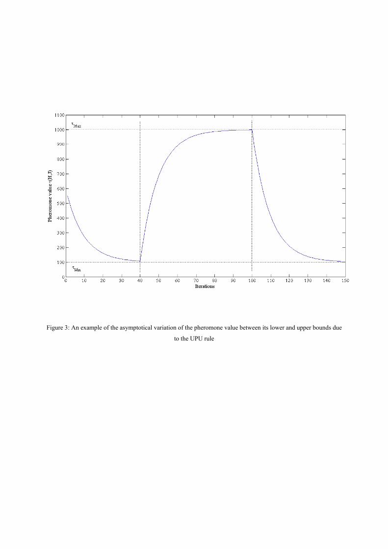
Figure 3: An example of the asymptotical variation of the pheromone value between its lower and upper bounds due

to the UPU rule

(a)

(b)

Figure 4: An example of the effect on the UPU rule of the two different options for defining *kΩ

-8

-6

-4

-2

0

2

4

6

8

111 011 001 101 100 010 000 110

Figure 5: The average percentage deviations of the different configurations in Table 1 with the 95% confidence

intervals

-6

-5

-4

-3

-2

-1

0

1

2

3

111 001 011 101 010 110 000 100

Figure 6: The average percentage deviations of the different configurations in Table 2 with the 95% confidence

intervals