a new approach for estimating the seismic soil...
TRANSCRIPT

Transaction A: Civil EngineeringVol. 17, No. 4, pp. 273{284c Sharif University of Technology, August 2010
A New Approach for Estimating theSeismic Soil Pressure on Retaining Walls
S. Maleki1;� and S. Mahjoubi1
Abstract. In this paper, a simple �nite element model for seismic analysis of retaining walls isintroduced. The model incorporates nonlinearity in the behavior of near wall soil, wall exibility andelastic free �eld soil response. This model can be employed in nonlinear modeling of retaining walls andbridge abutments. The advantages of this model are simplicity and exibility in addition to acceptableprecision. Using this �nite element model, an analytical study is conducted on several soil-wall systemsusing nonlinear time-history analysis by applying real earthquake records. Based on the results of theseanalyses, new seismic soil pressure distributions are proposed for di�erent soil and boundary conditions.These distributions are shown to be more accurate than the popular Mononobe-Okabe equations.
Keywords: Seismic analysis; Retaining walls; Soil pressure; Soil-structure interaction; Mononobe-Okabe; Finite element analysis.
INTRODUCTION
Seismic behavior of retaining walls has been widelyinvestigated by researchers since the 1920's. Threepioneer researchers in this �eld have been Mononobe,Matsuo and Okabe [1,2]. They proposed a pseudostatic method to calculate the seismically inducedactive and passive earth pressures using the Coulombtheory in a wedge of soil behind the wall. The method,herein called the M-O method, gives two relationshipsfor seismic active and passive earth pressures withlinear distribution along the wall height. Owing toits simplicity, this method has been widely used bypracticing engineers. Seed and Whitman [3] modi�edthe M-O method and suggested new relationships forthe seismic soil thrust in terms of unit weight of soil andpeak ground acceleration. They also suggested 0:6H asthe resultant force point of action where H is the heightof the retaining wall. Anderson et al. [4], by a series ofcentrifuge tests, found that the location of equivalentdynamic soil pressure forces varies, but recommendeda value of 0:5 H for its approximate location. Sherif etal. [5] and Wood [6] proposed a value of 0:45 H abovethe base for the seismic earth thrust point of action.
1. Department of Civil Engineering, Sharif University of Tech-nology, Tehran, P.O. Box 11155-9313, Tehran, Iran.
*. Corresponding author. E-mail: [email protected]
Received 14 September 2009; received in revised form 3 March2010; accepted 17 July 2010
Experimental studies since the 1970's have provedthat the M-O method and the modi�ed version (Seedand Whitman method) are satisfactory in calculatingthe total seismic soil thrust [4,5,7,8].
Another prevalent method used by engineers isthe subgrade modulus method. In this method, thesoil behind the wall is modeled as a series of parallelmassless springs. Using this concept, Scott [9] studiedthe soil-wall interaction. He modeled the free �eld soilas a vertical shear beam with mass and the interfacingsoil as massless linear springs with constant sti�ness.Veletsos and Younan [10] improved Scott's method byapplying semi-in�nite horizontal bars with constantmass per length connected to the wall by masslesslinear springs. Richards et al. [11], retrospectingScott and Veletsos and Younan studies, represented amethod of dynamic analysis for retaining walls using a2D model containing a semi-in�nite nonlinear layer ofcohesionless soil, free at the top and rigidly restrainedat the bottom. The retaining wall is connected tothe free �eld soil by means of elastic constant sti�nesssprings. They studied the model in four modes ofdisplacement: rotation about base, rotation abouttop, rigid translation and �xed base. Veletsos andYounan [12], using Lagrange's equation, analyzed alinear model and investigated the e�ects of manyvariables, such as base �xity and nonuniformity of thesoil shear modulus, on the soil thrust. They concludedthat for realistic wall exibilities, the total wall force is
274 S. Maleki and S. Mahjoubi
one half or less of that obtained for a �xed base, rigidwall. They also found the elastic method to be of goodprecision.
Recently, with great progress in computer soft-ware and hardware, nonlinear models have been usedby several researchers to investigate many aspects ofsoil-wall interaction and wall behavior during earth-quakes [13-15]. Green and Ebling [16] employed anelasto-plastic constitutive model for the soil in con-junction with the Mohr-Coulomb failure criterion. Thewall is modeled with elastic beam elements using acracked second moment of inertia. Interface elementswere used to model the wall-soil interface. Cheng [17]proposed relationships for calculating seismic lateralearth pressure coe�cients for cohesive soils using theslip line method. He found iterative analysis tobe useful for obtaining passive earth pressure butunimportant for active earth pressure. He also foundthat active earth pressure is much more in uencedby the PGA of an earthquake than passive pressure.Psarropoulos et al. [18] used a �nite-element model tostudy the dynamic earth pressures developed on rigidor exible nonsliding retaining walls modeling the soilas a viscoelastic continuum. Results showed a crudeconvergence between the M-O and elasticity-basedsolutions for structurally or rotationally exible walls.
More recently, Choudhury and Chatterjee [19], asan extension of the Veletsos and Younan study, used amass-spring-dashpot dynamic model with two degreesof freedom to arrive at the total active earth pressureunder earthquake time history loading. They suggestedthe use of an in uence zone of 10 times the wall heightfor the soil media behind the wall for dynamic models.They also presented non dimensional design charts forrapid calculation of active earth pressures. Choudhuryand Subba Rao, in two di�erent studies, obtained anestimate for the seismic passive earth pressure againstretaining walls by using logarithmic spiral and com-posite curve failure surface assumptions and a pseudostatic method [20,21]. E�ects of cohesion, surcharge,own weight, wall batter angle, ground surface slope, soilfriction angle and seismic accelerations were consideredin the analysis.
Although, nowadays, many commercial computerprograms with the ability to perform nonlinear anal-ysis of continua are available, these programs areexpensive and time-consuming in nonlinear stepwiseanalyses. Uncertainty regarding the input for soil pa-rameters is also a drawback. Programs like FLAC [22],SHAKE [23] and SASSI [24] are simpler than thegeneral purpose �nite element software, but each hasits own limitations.
The objective of this paper is to obtain a simpli-�ed seismic soil pressure distribution against retainingwalls with di�erent boundary and sti�ness conditions,such as rigid walls, exible walls, bridge abutments and
propped bridge abutments. Nonlinear �nite elementdynamic time history analyses of soil-wall systems areemployed for veri�cation. It is shown that the sug-gested equations more accurately predict the seismicsoil pressure behind retaining walls than the well-known M-O relationships, and are simple to use.
SOIL-WALL MODEL
In this section, the theoretical background for con-struction of an accurate �nite element soil-wall analysismodel is described. Past research has been selectivelyput together to obtain a simple but yet accuratemodel that ignores nonlinearity in the far �eld soil butcaptures it in the near �eld soil adjacent to the wallwhere it most a�ects the wall pressure.
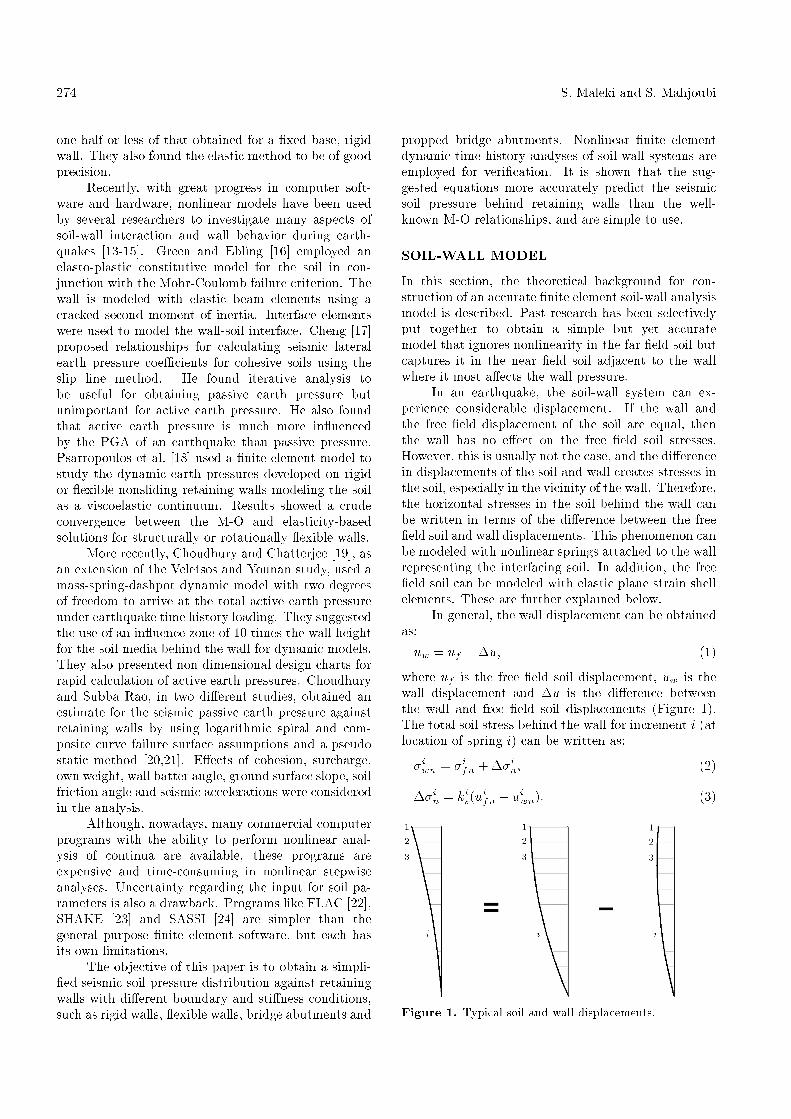
In an earthquake, the soil-wall system can ex-perience considerable displacement. If the wall andthe free �eld displacement of the soil are equal, thenthe wall has no e�ect on the free �eld soil stresses.However, this is usually not the case, and the di�erencein displacements of the soil and wall creates stresses inthe soil, especially in the vicinity of the wall. Therefore,the horizontal stresses in the soil behind the wall canbe written in terms of the di�erence between the free�eld soil and wall displacements. This phenomenon canbe modeled with nonlinear springs attached to the wallrepresenting the interfacing soil. In addition, the free�eld soil can be modeled with elastic plane strain shellelements. These are further explained below.
In general, the wall displacement can be obtainedas:uw = uf ��u; (1)
where uf is the free �eld soil displacement, uw is thewall displacement and �u is the di�erence betweenthe wall and free �eld soil displacements (Figure 1).The total soil stress behind the wall for increment i (atlocation of spring i) can be written as:
�iwn = �ifn + ��in; (2)
��in = kis(uifn � uiwn): (3)
Figure 1. Typical soil and wall displacements.

Seismic Soil Pressure on Retaining Walls 275
�iwn = total soil normal stress against the wall atincrement i (at location of spring i).
�ifn = normal soil stress in free �eld atincrement i.
��in = variation of soil stress because of thedi�erence between the free �eld soil andwall displacements at increment i.
kis = soil subgrade modulus at increment i.
The total horizontal force behind the wall is:
Pnt =Z H
0�wndz; (4)
and the overturning moment is:
Mnt =Z H
0�wnzdz: (5)
Therefore, the point of application of the resultanthorizontal force is obtained as:
h0 =Mnt
Pnt: (6)
For cohesionless soils, the modulus of elasticity (E) andthe shear modulus (G) vary increasingly with depth.Two common assumptions for this variation are linearand parabolic. Here, the parabolic assumption is usedfor the shear modulus as follows [11]:
Gz = GH :pz=H; (7)
whereGz andGH are the elastic shear moduli at depthsz and H, respectively.
The soil behind the wall is divided into layers andthe above equation is used to estimate G in the middleof each layer. The equivalent springs representing thesoil adjacent to the wall are modeled using nonlinearlink elements. The sti�ness of each spring, de�ned asthe subgrade modulus, is derived as follows [9]:
ks = Cz:GzH; (8)
where Cz is a constant representing the geometricproperties of the model. The value of Cz is assumed
to be 1.35 based on the suggestion of Huang [11,25].Soil pressure is considered bounded by the active andpassive soil pressures as follows:
Ka: :z � �z � Kp: :z; (9)
where:
Ka =1� sin�1 + sin�
; Kp =1 + sin�1� sin�
: (10)
Therefore, the springs between the free �eld soil andretaining wall are modeled as a bilinear elastic perfectlyplastic type. The initial elastic linear part sti�nessis calculated from Equation 8 by substituting Gz foreach spring from Equation 7. The plastic portion has amaximum/minimum force of Pp=Pa. These are springforces equivalent to passive and active soil pressures,respectively, and are calculated by multiplying passiveor active soil pressures and the spring correspondingarea for each spring. A typical force-displacement plotfor soil springs between the retaining wall and the free�eld soil is shown in Figure 2.
Figure 3 shows the structural model of the soil-wall system. The wall is modeled by using shellelements of concrete. The width of the wall and soilshell elements, perpendicular to the paper in Figure 3,is considered to be 1 meter.
The free �eld soil modeling in this study consistsof an in�nite half-space elastic layer of dense cohesion-less soil with unit weight of . This half-space layer
Figure 2. Typical force-displacement plot for soil springsbehind a retaining wall.
Figure 3. Soil-wall �nite element model.
276 S. Maleki and S. Mahjoubi
is free at the top and considered �xed at the bottomwhere similar soil acceleration is applied to the soil andwall during an earthquake. Free �eld soil is assumed tohave a �nite length equal to 4 to 5 times its thickness.Choudhury and Chatterjee suggested an in uence zoneof 10 times the wall height for the soil media behindthe wall [19]. However, in their study, soil media atthe end is not restrained against vertical displacement,which is the case in this study (Figure 3). The authorsfound that restraining the end of the soil media againstvertical displacement decreases the in uence zone andmakes the model smaller and more e�cient.
The height of the retaining wall and the soilbehind it are assumed to be the same and equal to H.The free �eld soil layer is modeled using plane strainelements. Soil layers have di�erent elastic properties;however, they are assumed to be constant within eachsoil layer. Shear modulus is calculated by substitutingthe average depth of the layer as z in Equation 7.Poisson's ratio for all soil layers is assumed to be 0.3.
Four di�erent cases of rigid retaining wall, exiblecantilever retaining wall, bridge abutment and proppedbridge abutment are considered, each with 4 m, 6 mand 8 m wall heights. In the case of a rigid retainingwall, it is assumed that the wall has unlimited sti�nessand so shows no deformation. Although in reality thisis impossible, the case of a buttressed wall comes veryclose to this assumption.
The exible wall case is the case of a cantileverretaining wall with variable thickness. It is assumedthat the thickness varies from 0.3 m at the top to 0:1 Hat the bottom. In the case of a 4 m exible wall, it isnot practical to vary the wall thickness from 0.3 m to0.4 m. Therefore, the wall thickness is considered to beconstant and equal to 0.4 m.
In the case of bridge abutments, the wall thicknessis considered to be constant throughout the height.The thickness is assumed to be equal to 1 m for 6 m and8 m height walls and 0.8 m for a 4 m height wall. Thecase of a propped bridge abutment is a special case ofbridge abutment in which the superstructure restrainsthe abutment horizontally at the top. Although inreality this restraining is limited, the case is valuableas an extreme boundary condition case.
In all cases considered for analyses, the wall isfully restrained at the bottom (rotations and displace-ments). However, the e�ect of foundation rotationalsti�ness is investigated separately for a 6 m high bridgeabutment and the propped bridge abutment models.In these models, the restraint against rotation at thebottom of the wall is removed and a rotational spring issubstituted to model the foundation and soil rotationalsti�ness.
In bridge structures, the superstructure connec-tion to the abutment can be categorized into twomain groups: free and restrained. If the super-
structure is not restrained to the abutment, the gapbetween the backwall and the superstructure is usuallyclosed by the superstructure movements and, mostof the time, the collision of the superstructure intothe backwall is unavoidable in severe earthquakes.This collision produces a considerable concentratedforce at the top of the bridge abutment. In thesecond case where the superstructure is restrainedto the abutment, the superstructure inertial force istransferred to the abutment through the restraintas a concentrated force at the abutment seat level.Therefore, abutments have to resist a considerableconcentrated force at their top during earthquakes inboth cases. However, the e�ect of a superstructurehorizontal force on top of the abutment is usuallyignored in bridge abutment design. To evaluatethe e�ect of this force and determine the part ofthis force taken by the soil behind the abutment, aconcentrated force with variable value is consideredto push the wall against the soil at the assumedsuperstructure center of mass, as is the case duringearthquakes.
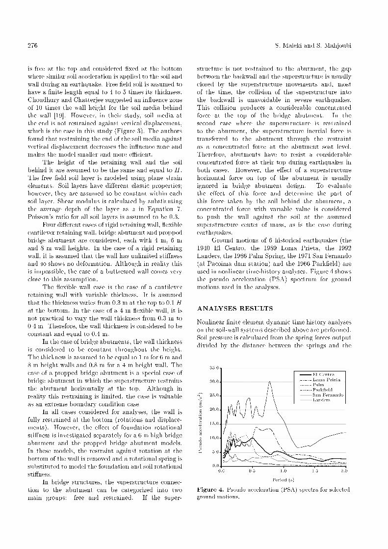
Ground motions of 6 historical earthquakes (the1940 El Centro, the 1989 Loma Prieta, the 1992Landers, the 1986 Palm Spring, the 1971 San Fernando(at Pacoima dam station) and the 1966 Park�eld) areused in nonlinear time-history analyses. Figure 4 showsthe pseudo acceleration (PSA) spectrum for groundmotions used in the analyses.
ANALYSES RESULTS
Nonlinear �nite element dynamic time history analyseson the soil-wall systems described above are performed.Soil pressure is calculated from the spring forces outputdivided by the distance between the springs and the
Figure 4. Pseudo acceleration (PSA) spectra for selectedground motions.
Seismic Soil Pressure on Retaining Walls 277
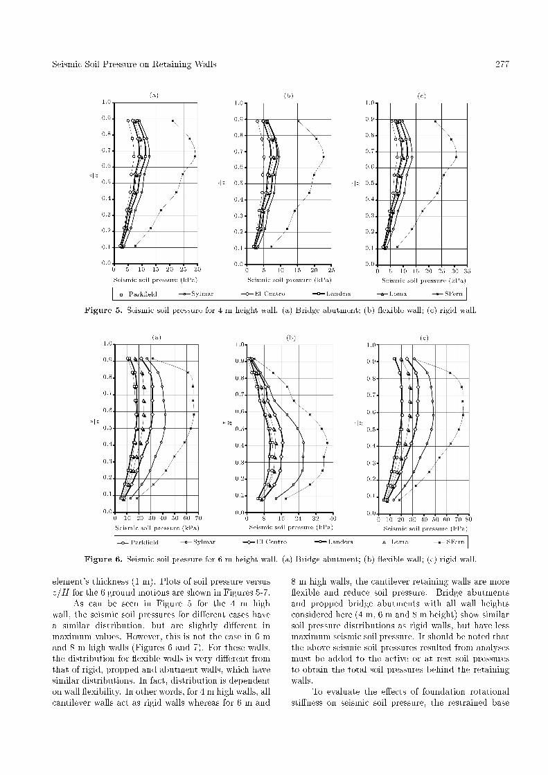
Figure 5. Seismic soil pressure for 4 m height wall. (a) Bridge abutment; (b) exible wall; (c) rigid wall.
Figure 6. Seismic soil pressure for 6 m height wall. (a) Bridge abutment; (b) exible wall; (c) rigid wall.
element's thickness (1 m). Plots of soil pressure versusz=H for the 6 ground motions are shown in Figures 5-7.
As can be seen in Figure 5 for the 4 m highwall, the seismic soil pressures for di�erent cases havea similar distribution, but are slightly di�erent inmaximum values. However, this is not the case in 6 mand 8 m high walls (Figures 6 and 7). For these walls,the distribution for exible walls is very di�erent fromthat of rigid, propped and abutment walls, which havesimilar distributions. In fact, distribution is dependenton wall exibility. In other words, for 4 m high walls, allcantilever walls act as rigid walls whereas for 6 m and
8 m high walls, the cantilever retaining walls are more exible and reduce soil pressure. Bridge abutmentsand propped bridge abutments with all wall heightsconsidered here (4 m, 6 m and 8 m height) show similarsoil pressure distributions as rigid walls, but have lessmaximum seismic soil pressure. It should be noted thatthe above seismic soil pressures resulted from analysesmust be added to the active or at rest soil pressuresto obtain the total soil pressures behind the retainingwalls.
To evaluate the e�ects of foundation rotationalsti�ness on seismic soil pressure, the restrained base
278 S. Maleki and S. Mahjoubi
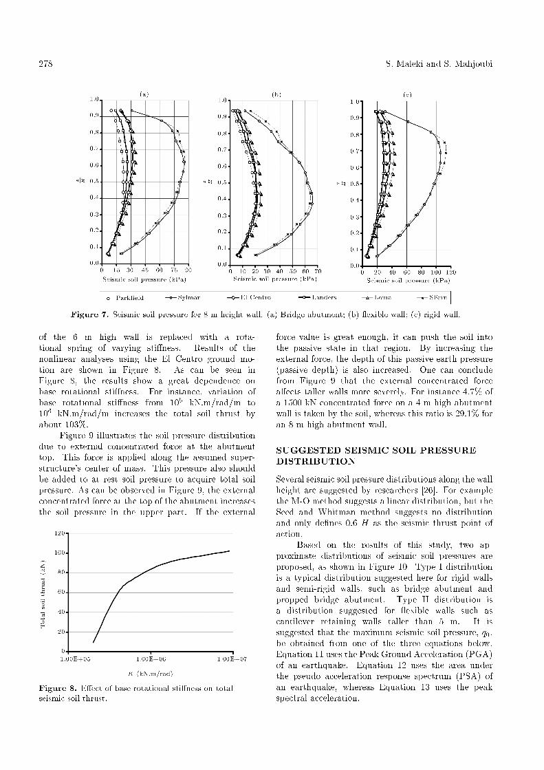
Figure 7. Seismic soil pressure for 8 m height wall. (a) Bridge abutment; (b) exible wall; (c) rigid wall.
of the 6 m high wall is replaced with a rota-tional spring of varying sti�ness. Results of thenonlinear analyses using the El Centro ground mo-tion are shown in Figure 8. As can be seen inFigure 8, the results show a great dependence onbase rotational sti�ness. For instance, variation ofbase rotational sti�ness from 105 kN.m/rad/m to106 kN.m/rad/m increases the total soil thrust byabout 103%.
Figure 9 illustrates the soil pressure distributiondue to external concentrated force at the abutmenttop. This force is applied along the assumed super-structure's center of mass. This pressure also shouldbe added to at rest soil pressure to acquire total soilpressure. As can be observed in Figure 9, the externalconcentrated force at the top of the abutment increasesthe soil pressure in the upper part. If the external
Figure 8. E�ect of base rotational sti�ness on totalseismic soil thrust.
force value is great enough, it can push the soil intothe passive state in that region. By increasing theexternal force, the depth of this passive earth pressure(passive depth) is also increased. One can concludefrom Figure 9 that the external concentrated forcea�ects taller walls more severely. For instance 4.7% ofa 1500 kN concentrated force on a 4 m high abutmentwall is taken by the soil, whereas this ratio is 29.1% foran 8 m high abutment wall.
SUGGESTED SEISMIC SOIL PRESSUREDISTRIBUTION
Several seismic soil pressure distributions along the wallheight are suggested by researchers [26]. For examplethe M-O method suggests a linear distribution, but theSeed and Whitman method suggests no distributionand only de�nes 0:6 H as the seismic thrust point ofaction.
Based on the results of this study, two ap-proximate distributions of seismic soil pressures areproposed, as shown in Figure 10. Type I distributionis a typical distribution suggested here for rigid wallsand semi-rigid walls, such as bridge abutment andpropped bridge abutment. Type II distribution isa distribution suggested for exible walls such ascantilever retaining walls taller than 5 m. It issuggested that the maximum seismic soil pressure, q0,be obtained from one of the three equations below.Equation 11 uses the Peak Ground Acceleration (PGA)of an earthquake. Equation 12 uses the area underthe pseudo acceleration response spectrum (PSA) ofan earthquake, whereas Equation 13 uses the peakspectral acceleration.

Seismic Soil Pressure on Retaining Walls 279
Figure 9. Force-induced soil pressure. (a) 4 m bridge abutment; (b) 6 m bridge abutment; (c) 8 m bridge abutment.
Figure 10. Suggested approximate seismic soil pressuredistributions. (a) Type I; (b) Type II.
q0 = �:kh: :H; (11)
q0 = �1:A0: :H; (12)
q0 = �2:S: :H; (13)
where:
q0 = maximum seismic soil pressure.kh = seismic horizontal acceleration coe�cient.A0 = the area under the PSA spectrum between
0:2T and 1:5T in which T is the period of the�rst mode of vibration (the spectrummust be in units of m/s2).
S = Spectral acceleration in units of m/s2
obtained from the PSA spectrum of anearthquake at the period of vibration forthe �rst mode of the soil-wall system.
�, �1 and �2 are coe�cients from Tables 1 to 3,
Table 1. Coe�cient � and distribution type in � method.
Case Distribution �
Bridge abutment (H < 5 m) I 0.31
Bridge abutment (H � 5 m) I 0.55
Rigid and propped wall (H < 5 m) I 0.32
Rigid and propped wall (H � 5 m) I 0.64
RC retaining wall (H < 5 m) I 0.25
RC retaining wall (H � 5 m) II 0.44
Table 2. Coe�cient �1 and distribution type in �1
method.Case Distribution �1
Bridge abutment, rigid wall, and
propped wall (independent of height)
& RC retaining wall (H < 5 m)
I 0.13
RC retaining wall (H � 5 m) II 0.07
Table 3. Coe�cient �2 and distribution type in �2
method.Case Distribution �2
Bridge abutment (H < 5 m) I 0.018
Bridge abutment (H � 5 m) I 0.03
Rigid and propped Wall (H<5 m) I 0.019
Rigid and propped Wall (H�5 m) I 0.035
RC retaining wall (H < 5 m) I 0.015
RC retaining wall (H � 5 m) II 0.020

280 S. Maleki and S. Mahjoubi
adjusting the pressure for wall height and boundarycondition.
Distribution type (I or II) shown in Figure 10 isalso de�ned in Tables 1 to 3 for each case with di�erentwall heights and boundary conditions.
Seismic soil pressure distributions introducedabove are based on the results of analyses on �xedbased models for two reasons. Firstly, to simplifydistributions and their corresponding relationships, sothat they are independent of soil sti�ness, foundationsti�ness and foundation width which could complicatethe relationships and make them undesirable for de-sign. Secondly, to arrive at a conservative estimatefor pressure distributions suitable for design purposes.A �xed-based wall absorbs much more seismic soilpressure than a wall with �nite base rotational sti�ness.It should be noted that the base rotational �xity isnot unreal. For example, the case of pile foundations(usually used in bridge abutments) is very close to baserotational �xity.
Many earthquake records with di�erent intensitiesand frequency contents and di�erent soil types maybe used along with the proposed method suggestedin this paper. However, this is deemed unnecessarybecause the suggested method shows good accordancewith other reliable studies in most cases.
The q0 obtained from Equation 11, which is calledthe � method herein, is less accurate in comparisonwith the other two relationships (Equations 12 and 13).This is because the PGA is the simplest and mostavailable parameter of an earthquake and ignores theother characteristics of ground motion. Equations 12and 13, herein called the �1 and the �2 methods, givemore accurate results but require the PSA spectrumof the input ground motion. In using the � methods,one needs the period of the �rst mode of vibration(T ) for a soil-wall system. Based on the results ofmodal analyses of several soil-wall systems, the authorssuggest Equation 14 or Figure 11 to rapidly obtain Twithout analysis:
T = 0:0029H2 � 0:0062H + 0:142; (14)
where H is the wall height and is restricted between 3to 10 meters.
Note that for design purposes, the design responsespectrum and the PGA of any local seismic designcodes can be used as input in � and � methods,respectively.
Total seismic soil thrust against a retaining wall(PST ) for proposed distributions can be obtained as:
Distribution I:
PST =23q0H: (15)
Figure 11. Period of the �rst mode of vibration (T ) forsoil-wall systems.
Distribution II:
PST =35q0H: (16)
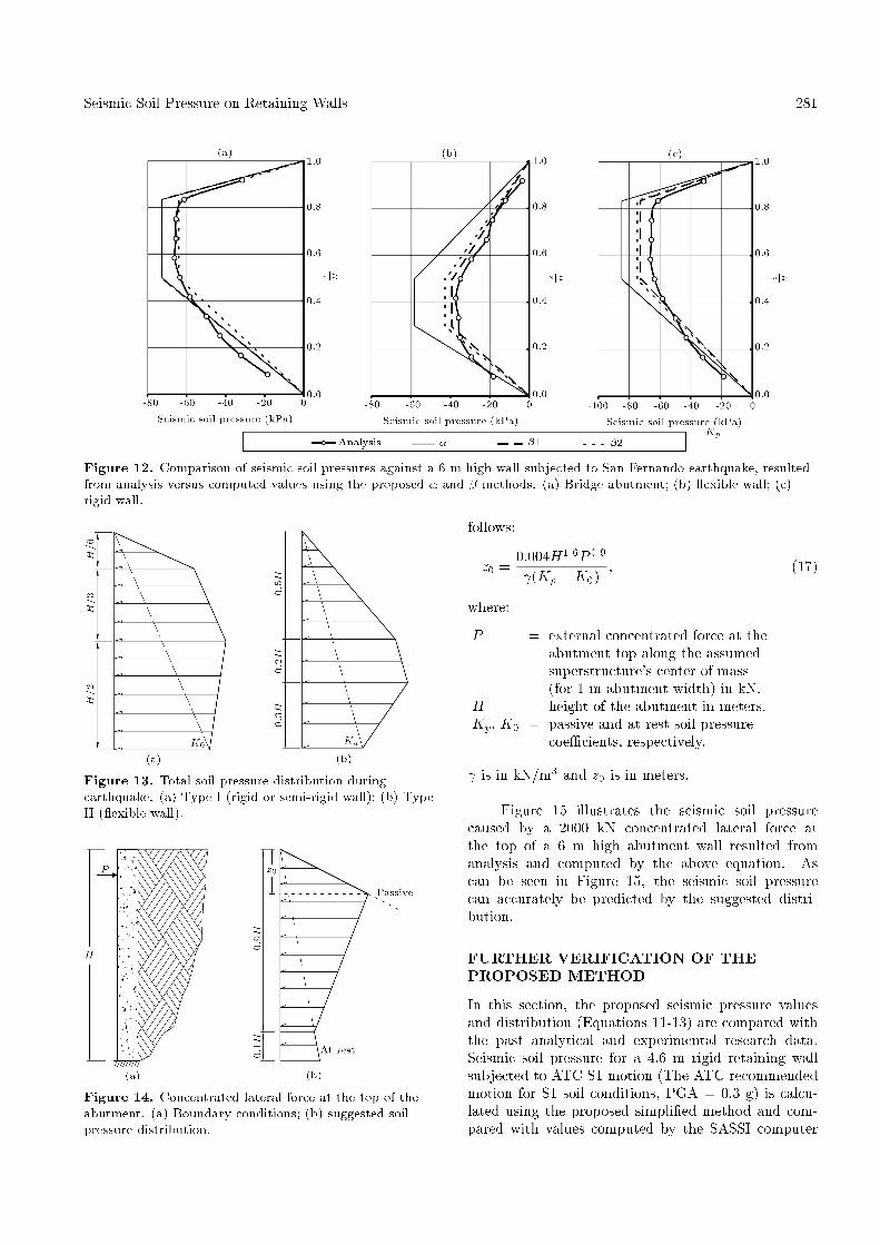
Figure 12 shows the seismic soil pressures against a 6 mhigh wall subjected to the San Fernando earthquake,resulted from analyses in di�erent cases. Suggesteddistributions for seismic soil pressure using the � and� methods are also shown for comparison. As canbe seen in Figure 12, the seismic soil pressure is bestpredicted by the �1 method. The � method, althoughshowing more dispersion, gives acceptable results fordesign purposes. It can also be observed that thesuggested distributions are in good agreement withthe distributions of seismic soil pressure results fromtime history analyses of di�erent cases under di�erentearthquakes.
The seismic soil pressures introduced aboveshould be added to the active or at rest soil pressures toacquire the total soil pressure. For rigid and semi-rigidwalls (such as bridge abutment and propped bridgeabutment), at rest soil pressure is more appropriate,whereas for exible walls, such as cantilever retainingwalls higher than 5 m, active soil pressure should beadded to suggested distributions. Figure 13 showstypical total soil pressure distributions for the two casesdiscussed.
For the case of concentrated lateral force at thetop of the abutment (Figure 14a), which usually occursin bridges during earthquakes, a new distribution forsoil pressure is herein introduced and is illustrated inFigure 14b. This distribution has only one parameter,z0, which is the passive depth de�ned above. Thedistribution in depths less than z0 follows the passivesoil pressure and at depths more than 0:9 H followsthe at rest soil pressure. Between depths z0 and 0:9H,soil pressure linearly decreases from passive to at restsoil pressure. The depth ratio, z0, can be obtained as
Seismic Soil Pressure on Retaining Walls 281
Figure 12. Comparison of seismic soil pressures against a 6 m high wall subjected to San Fernando earthquake, resultedfrom analysis versus computed values using the proposed � and � methods. (a) Bridge abutment; (b) exible wall; (c)rigid wall.
Figure 13. Total soil pressure distribution duringearthquake. (a) Type I (rigid or semi-rigid wall); (b) TypeII ( exible wall).
Figure 14. Concentrated lateral force at the top of theabutment. (a) Boundary conditions; (b) suggested soilpressure distribution.
follows:
z0 =0:004H1:6P 0:9
(Kp �K0); (17)
where:
P = external concentrated force at theabutment top along the assumedsuperstructure's center of mass(for 1 m abutment width) in kN.
H = height of the abutment in meters.Kp, K0 = passive and at rest soil pressure
coe�cients, respectively.
is in kN/m3 and z0 is in meters.
Figure 15 illustrates the seismic soil pressurecaused by a 2000 kN concentrated lateral force atthe top of a 6 m high abutment wall resulted fromanalysis and computed by the above equation. Ascan be seen in Figure 15, the seismic soil pressurecan accurately be predicted by the suggested distri-bution.
FURTHER VERIFICATION OF THEPROPOSED METHOD
In this section, the proposed seismic pressure valuesand distribution (Equations 11-13) are compared withthe past analytical and experimental research data.Seismic soil pressure for a 4.6 m rigid retaining wallsubjected to ATC S1 motion (The ATC recommendedmotion for S1 soil conditions, PGA = 0.3 g) is calcu-lated using the proposed simpli�ed method and com-pared with values computed by the SASSI computer

282 S. Maleki and S. Mahjoubi
Figure 15. Seismic soil pressure caused by a 2000 kNconcentrated lateral force at the top of a 6 m highabutment wall, resulted from analyses and computed byproposed method.
program [24], M-O active earth pressure (using kh =0:3, kv = 0) and the Ostadan proposed method [27].The results are shown in Figure 16a. As can be seenin Figure 16a, seismic soil pressure values computedby the proposed method are in good accordance withthe two other seismic pressure values and are less thanthe M-O active earth pressure at depths of more than0:6H.
In addition, to verify the proposed seismic soilpressure distribution, normalized seismic soil pressure(soil pressure normalized to 1 at the bottom of the wallfor pressure distribution type I) is plotted in Figure 16bagainst z=H (normalized depth) and compared withthe normalized seismic soil pressures presented by theM-O, Wood [6], Ostadan [27], Veletsos and Younan(rigid wall) [12] methods, and also results from theshaking table tests performed by Ohara and Maehara(rigid wall- case compound displacement II) [28] andrecently performed centrifuge tests by Nakamura (rigidwall- case 21) [29]. Figure 16b shows that the proposedseismic soil pressure distribution is in good agreementwith analytical methods and experimental data pre-sented in the literature.
SUMMARY AND CONCLUSIONS
In this paper, a method for modeling retaining wall sys-tems was proposed. The model includes free �eld soil,a retaining wall and springs modeling the interfacingsoil. The method is exible enough to be used underdi�erent soil and wall conditions and has satisfactoryprecision. The popular M-O method's assumptions,such as a rigid gravity wall and a rigid wedge of soil
Figure 16. (a) Comparison of proposed seismic soilpressure and computed values with SASSI program andOstadan method for a 4.6 m wall, ' = 30�, ATC motion.(b) Comparison of proposed seismic soil pressuredistribution with analytical and experimentaldistributions [6,12,27-29].
sliding on a linear failure surface, can be criticized,in most cases. This paper's modeling technique isapplicable to rigid and exible walls with di�erentend conditions. Using this model, nonlinear dynamic�nite element time history analyses were performedon several soil-wall systems to arrive at the followingconclusions:
1. Comparing the results of analyses with the modi�edM-O [3] method shows that the M-O method isnot accurate in every case, but, on average, givesacceptable results for practical purposes.
Seismic Soil Pressure on Retaining Walls 283
2. The notion that the seismic soil pressure increaseswith increasing PGA of an earthquake is not truein every case. It is found that seismic soil pressureis more closely related to the area under the PSAspectrum than the peak ground acceleration of anearthquake.
3. For cantilever walls, seismic soil pressure is greatlyin uenced by the value of the base rotationalsti�ness. Maximum soil pressure happens for rigid�xed-base walls.
4. Bridge abutments and propped bridge abutmentsshow similar soil pressure distributions as of rigidwalls, but the peak seismic soil pressure is less.
5. Three di�erent methods were proposed for seismicsoil pressure distribution against retaining walls(Equations 11-13). These methods are simple touse and show good agreement with nonlinear �niteelement analyses results, and also past analyticaland experimental research data.
6. For the case of a concentrated load applied at thetop of an abutment, a simple pressure distributionwas also presented (Equation 17).
7. An equation for estimating the �rst mode periodof vibration for the soil-wall system was introduced(Equation 14).
REFERENCES
1. Mononobe, N. and Matsuo, H. \On the determinationof earth pressures during earthquakes", Proc. WorldEngrg. Conf., 9, paper No. 388, pp. 177-185 (1929).
2. Okabe, S. \General theory of earth pressure", J.Japanese Soc. of Civ. Engrs., 12(1) (1926).
3. Seed, H.B. and Whitman, R.V. \Design of earthretaining structures for dynamic loads", The SpecialtyConference on Lateral Stresses in the Ground andDesign of Earth Retaining Structures, ASCE, pp. 103-147 (1970).
4. Andersen, G.R., Whitman, R.V. and Geremaine, J.T.\Tilting response of centrifuge-modeled gravity retain-ing wall to seismic shaking", Report 87-14, Depart-ment of Civil Engineering, M.I.T. Cambridge, MA(1987).
5. Sherif, M.A., Ishibashi, I. and Lee, C.D. \Earthpressures against rigid retaining walls", J. Geotech.Engrg. Div., ASCE, 108(5), pp. 679-695 (1982).
6. Wood, J.H. \Earthquake induced soil pressures onstructures", Doctoral Dissertation, EERL 73-05, Cali-fornia Institute of Technology, Pasadena, CA (1973).
7. Ishibashi, I. and Fang, Y.S. \Dynamic earth pressureswith di�erent wall movement modes, soils and founda-tions", Japanese Soc. of Soil Mech. and Found. Engrg.,27(4), pp. 11-22 (1987).
8. Finn, W.D., Yodendrakumar, M., Otsu, H. and Steed-man, R.S. \Seismic response of a cantilever retainingwall", 4th Int. Conf. on Soil Dyn. and EarthquakeEngrg., Southampton, pp. 331-431 (1989).
9. Scott, R.F. \Earthquake-induced pressures on retain-ing walls", 5th World Conf. on Earthquake Engrg. Int.Assn. of Earthquake Engrg., 2, Tokyo, Japan, pp.1611-1620 (1973).
10. Veletsos, A.S. and Younan, A.H. \Dynamic modelingand response of soil-wall systems", J. Geotech. Engrg.,ASCE, 120(12), pp. 2155-2179 (1994).
11. Richards, R.J., Huang, C. and Fishman, K.L. \Seismicearth pressure on retaining structures", J. Geotech.Engrg., ASCE, 125(9), pp. 771-778 (1999).
12. Veletsos, A.S. and Younan, A.H. \Dynamic response ofcantilever retaining walls", J. Geotech and GeoenvironEngng, ASCE, 123, pp. 161-172 (1997).
13. El-Emam, M.M., Bathurst, R.J. and Hatami, K.\Numerical modeling of reinforced soil retaining wallssubjected to base acceleration", Proc. 13th WorldConference on Earthquake Engineering, Vancouver,BC, paper No. 2621 (2004).
14. Green, R.A. and Ebeling, R.M. \Seismic analysis ofcantilever retaining walls", Phase I, ERDC/ITL TR-02-3. Information Technology Laboratory, US ArmyCorps of Engineers, Engineer Research and Develop-ment Center, Vicksburg, MS, USA (2002).
15. Puri, V.K., Prakas, S. and Widanarti, R. \Retainingwalls under seismic loading", Fifth International Con-ference on Case Histories in Geotechnical Engineering,New York, NY, USA (2004).
16. Green, R.A. and Ebeling, R.M. \Modeling the dy-namic response of cantilever earth-retaining walls usingFLAC", 3rd International Symposium on FLAC: Nu-merical Modeling in Geomechanics, Sudbury, Canada(2003).
17. Cheng, Y.M. \Seismic lateral earth pressure coe�-cients for c � ' soils by slip line method", Computersand Geotechnics, 30(8), pp. 661-670 (2003).
18. Psarropoulos, P.N., Klonaris, G. and Gazetas, G.\Seismic earth pressures on rigid and exible retainingwalls", Soil Dyn. and Earthquake Engng., 25, pp. 795-809 (2004).
19. Choudhury, D. and Chatterjee, S. \Dynamic activeearth pressure on retaining structures", Sadhana,Academy Proceedings in Engineering Sciences, 31(6),pp. 721-730 (2006).
20. Choudhury, D. and Subba Rao, K.S. \Seismic passiveresistance in soils for negative wall friction", CanadianGeotechnical Journal, 39(4), pp. 971-981 (2002).
21. Subba Rao, K.S. and Choudhury, D. \Seismic passiveearth pressures in soils", Journal of Geotechnical andGeoenvironmental Engineering, ASCE, 131(1), pp.131-135 (2005).
22. Itasca Consulting Group, Inc. \FLAC (Fast La-grangian Analysis of Continua) user's manuals", Min-neapolis, MN, USA (2000).

284 S. Maleki and S. Mahjoubi
23. Schnabel, P.B., Lysmer, J. and Seed, H.B. \SHAKE-A computer program for earthquake response analysisof horizontally layered sites", Earthquake EngineeringResearch Center, University of California, Berkeley,California, USA (1972).
24. Lysmer, J., Ostadan, F. and Chen, C.C. \SASSI2000-A system for analysis of soil-structure interaction",University of California, Department of Civil Engineer-ing, Berkeley, California, USA (1999).
25. Huang, C. \Plastic analysis for seismic stress anddeformation �elds", PhD dissertation, Dept. of CivilEngrg., SUNY at Bu�alo, Bu�alo, NY, USA (1996).
26. Gazetas, G., Psarropoulos, P.N., Anastasopoulos, I.and Gerolymos, N. \Seismic behavior of exible retain-ing systems subjected to short-duration moderatelystrong excitation", Soil Dyn. and Earthquake Engng.,24, pp. 537-550 (2004).
27. Ostadan, F. \Seismic soil pressure for building walls:An updated approach", Soil Dynamics and EarthquakeEngineering, 25, pp. 785-793 (2005).
28. Ohara, S. and Maehara, H. \Experimental studiesof active earth pressure", Memoirs of the Faculty ofEngineering, Yamaguchi University, 20(1), pp. 51-64(1969).
29. Nakamura, S. \Reexamination of Mononobe-Okabetheory of gravity retaining walls using centrifuge modeltests", Soils and Foundations, 46(2), pp. 135-146(2006).
BIOGRAPHIES
Shervin Maleki obtained his BS and MS degreesfrom the University of Texas at Arlington with honors.
He then pursued his PhD degree in New MexicoState University at Las Cruces and �nished it in1988. He has many years of experience in structuraldesign, both in the US and Iran. He has beena faculty member at Bradley University in Illinoisand Sharif University of Technology in Iran. Hehas authored and/or coauthored over forty technicalpapers and has authored two books and a chapterin the Handbook of International Bridge Engineer-ing to be published in 2011. His research area ismainly focused on the Seismic Design of Bridges andBuildings. He has also patented a seismic damper inIran.
Saeed Mahjoubi started his university studies in2000 at Sharif University of Technology (SUT) in Iranin the �eld of Civil Engineering. Having �nishedhis undergraduate studies in 2004, he continued as agraduate student at SUT in Structural Engineering.He successfully defended his thesis entitled \SeismicBehavior of Integral Abutment Bridges" to obtain hisMS degree in 2006. He was accepted as a PhD studentat SUT in 2008. During his graduate studies heattended several international conferences to presenthis research which is mainly focused on Bridge SeismicAnalysis and Retro�t (Structural Engineering WorldCongress, Bangalore, 2007; 3rd International BridgeConference, Tehran, 2008, and 2 articles presented atthe 8th International Congress on Civil Engineering,Shiraz, 2009).