Journal of Applied Geophysics 136 (2017) 455–461

Contents lists available at ScienceDirect

Journal of Applied Geophysics

j ourna l homepage: www.e lsev ie r .com/ locate / j appgeo

A new approach for the interpretation of self-potential data by 2-Dinclined plate

Khalid S. Essa, Mahmoud Elhussein ⁎Geophysics Department, Faculty of Science, Cairo University, Giza, P.O. 12613, Egypt

⁎ Corresponding author.E-mail address: mahmoudelnouishy@yahoo.com (M. E

http://dx.doi.org/10.1016/j.jappgeo.2016.11.0190926-9851/© 2016 Elsevier B.V. All rights reserved.

a b s t r a c t

a r t i c l e i n f o

Article history:Received 25 April 2016Received in revised form 17 November 2016Accepted 19 November 2016Available online 21 November 2016

A new accurate technique has been developed to interpret self-potential (SP) data (d) measured along a profileby a two-dimensional (2-D) inclined plate-like body. The technique solves for the depth (z) to top and half-width(w) of the body, and is based on the second horizontal gradient (SHG) that is calculated at a number of windowlengths. Using points symmetrically distributed about the origin point of the SP profile, the scheme derives andevaluates a function F at various window lengths from the measured SP anomaly profile. At a fixed windowlength (s), the depth corresponding to an assumed half-width is determined by solving a nonlinear equation inthe formφ (d, s,w, z)=0. The depths corresponding to all consideredwindows are then obtained at the assumedwidth. The standard deviation of these depths is calculated for this width. This process is repeated for variouswidths. The final solution (the depth and half-width) of the interpretive buried structure is that which achievesthe least standard deviation. The validity and accuracy of the new scheme has been demonstrated on theoreticalnoise free and noisy SP data. It has been successfully applied to two real data, and it is found that the parametersestimated from the schemedescribed here are in good agreementwith those reported in the published literature.

© 2016 Elsevier B.V. All rights reserved.

Keywords:Self-potential data interpretationSecond horizontal gradient2-D inclined plateMineral exploration

1. Introduction

Self-potential (SP)method has a considerable importance inmineralexploration (Sundararajan et al., 1998; Essa et al., 2008; Mehanee,2014), engineering and environmental applications (Jardani et al.,2007; Hunter and Powers, 2008; Maineult, 2016), cave detection(Vichabian and Morgan, 2002), geothermal exploration (Zlotnicki andNishida, 2003; Minsley et al., 2008), archeological investigations(Wynn and Sherwood, 1984; Drahor et al., 1996; Cammarano et al.,1997; Drahor, 2004), and tracing paleo-shear zones within the conti-nental crust (Mehanee, 2015). The two-dimensional (2-D) inclinedsheet model is one of the most commonly used models to interpret SPanomalies generated by ore deposits (Roy and Chowdhury, 1959;Meiser, 1962; Paul, 1965; Rao et al., 1982; Rao and Babu, 1983; Murtyand Haricharan, 1985; Eppelbaum et al., 2004; Mehanee et al., 2011).

Several methods have been developed for the interpretation of SPanomalies caused by 2-D inclined plates. These methods can be classi-fied into two categories. Methods of Category I interpret the measuredSP data by some geometrically simple body (El-Araby, 2004; Pekşenet al., 2011; Biswas and Sharma, 2014; Mehanee, 2014, 2015) forwhich the direct (forward modeling) solution is defined by a closedform formula. The rationale is that some geologic settings have an iso-lated SP anomaly that can be interpreted by a single polarized body.Therefore, rapid interpretation techniques based on geometrically

lhussein).

simple shapes can be used and are useful in this context. Methods ofCategory II focus on 2- and three-dimensional (3-D) SP inversions forgeologic structures with arbitrary shape (Minsley et al., 2007;Mendonça, 2008). Rigorous 2- and 3-D SP inverse problem solving de-mands full forward modeling solution, high computational time and apriori information for the model parameters inverted for (Mehaneeet al., 2011). Furthermore, to the best of our knowledge all rigorous 2-and 3-D SP inversions (Minsley et al., 2007; Mendonça, 2008) thathave been published in the literature invert for the subsurface sourcecurrent distribution, not for the resistivity distribution (Minsley et al.,2007). These iterative inversions essentially demand knowing the sub-surface resistivity distribution in their forward modeling calculations.Hence, in order for these inversions to produce meaningful geologicalresults, these inversions must be supplemented with accurate a prioriinformation about the subsurface resistivity distribution that could beobtained from solving other inverse problems (e.g., using direct currentresistivity or electromagnetic data). The research presented in thispaper belongs to category I, and does not require large computationalresources nor a priori information about the subsurface resistivity distri-butions, which is essential in the 2- and 3-D SP source currentinversions.

Various approaches have been developed in the published literatureto interpret the SP anomalies caused by a 2-D inclined plate type anom-alous body. For example, graphical methods (Babu and Rao, 1988;Murty and Haricharan, 1985), logarithmic curve matching (Meiser,1962;Murty and Haricharan, 1984), and the use of characteristic points,distances and curves (Paul, 1965; Rao et al., 1970; Rao and Babu, 1983).

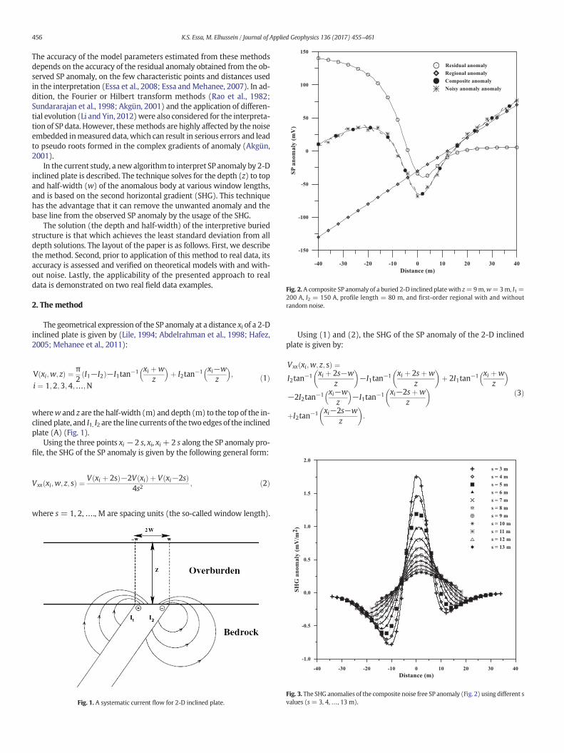
Fig. 2.A composite SP anomaly of a buried 2-D inclined plate with z=9m,w=3m, I1=200 A, I2 = 150 A, profile length = 80 m, and first-order regional with and withoutrandom noise.

456 K.S. Essa, M. Elhussein / Journal of Applied Geophysics 136 (2017) 455–461

The accuracy of the model parameters estimated from these methodsdepends on the accuracy of the residual anomaly obtained from the ob-served SP anomaly, on the few characteristic points and distances usedin the interpretation (Essa et al., 2008; Essa and Mehanee, 2007). In ad-dition, the Fourier or Hilbert transform methods (Rao et al., 1982;Sundararajan et al., 1998; Akgün, 2001) and the application of differen-tial evolution (Li and Yin, 2012)were also considered for the interpreta-tion of SP data. However, thesemethods are highly affected by the noiseembedded inmeasured data, which can result in serious errors and leadto pseudo roots formed in the complex gradients of anomaly (Akgün,2001).

In the current study, a new algorithm to interpret SP anomaly by 2-Dinclined plate is described. The technique solves for the depth (z) to topand half-width (w) of the anomalous body at various window lengths,and is based on the second horizontal gradient (SHG). This techniquehas the advantage that it can remove the unwanted anomaly and thebase line from the observed SP anomaly by the usage of the SHG.

The solution (the depth and half-width) of the interpretive buriedstructure is that which achieves the least standard deviation from alldepth solutions. The layout of the paper is as follows. First, we describethe method. Second, prior to application of this method to real data, itsaccuracy is assessed and verified on theoretical models with and with-out noise. Lastly, the applicability of the presented approach to realdata is demonstrated on two real field data examples.

2. The method

The geometrical expression of the SP anomaly at a distance xi of a 2-Dinclined plate is given by (Lile, 1994; Abdelrahman et al., 1998; Hafez,2005; Mehanee et al., 2011):

V xi;w; zð Þ ¼ π2

I1−I2ð Þ−I1tan−1 xi þwz

� �þ I2tan−1 xi−w

z

� �;

i ¼ 1;2;3;4;…;Nð1Þ

wherew and z are the half-width (m) and depth (m) to the top of the in-clined plate, and I1, I2 are the line currents of the two edges of the inclinedplate (A) (Fig. 1).

Using the three points xi − 2 s, xi, xi +2 s along the SP anomaly pro-file, the SHG of the SP anomaly is given by the following general form:

Vxx xi;w; z; sð Þ ¼ V xi þ 2sð Þ−2V xið Þ þ V xi−2sð Þ4s2

; ð2Þ

where s= 1, 2,…., M are spacing units (the so-called window length).

Fig. 1. A systematic current flow for 2-D inclined plate.

Using (1) and (2), the SHG of the SP anomaly of the 2-D inclinedplate is given by:

Vxx xi;w; z; sð Þ ¼I2tan−1 xi þ 2s−w

z

� �−I1tan−1 xi þ 2sþw

z

� �þ 2I1tan−1 xi þw

z

� �

−2I2tan−1 xi−wz

� �−I1tan−1 xi−2sþw

z

� �

þI2tan−1 xi−2s−wz

� �:

ð3Þ

Fig. 3. The SHG anomalies of the composite noise free SP anomaly (Fig. 2) using different svalues (s = 3, 4,…, 13 m).

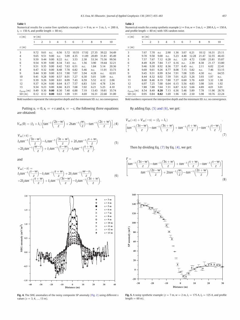
Table 1Numerical results for a noise free synthetic example (z = 9 m, w = 3 m, I1 = 200 A,I2 = 150 A, and profile length = 80 m).

s (m) w (m)

1 2 3 4 5 6 7 8 9 10

z (m)

3 9.72 9.61 n.c. 6.56 5.72 10.55 17.92 27.35 39.22 54.494 9.65 9.51 9.00 n.c. 5.09 4.35 11.89 20.89 31.81 45.495 9.59 9.44 9.00 8.22 n.c. 3.53 2.38 53.34 73.36 99.566 9.54 9.39 9.00 8.34 7.43 n.c. 1.56 3.90 19.44 32.217 9.51 9.35 9.00 8.42 7.63 6.51 n.c. 1.84 5.14 20.368 9.47 9.32 9.00 8.48 7.78 6.82 5.46 n.c. 11.91 33.739 9.44 9.30 9.00 8.53 7.90 7.07 5.94 4.28 n.c. 62.0110 9.41 9.28 9.00 8.57 8.01 7.27 6.30 5.01 3.09 n.c.11 9.39 9.26 9.00 8.61 8.09 7.43 6.59 5.52 4.12 2.0612 9.37 9.24 9.00 8.64 8.17 7.57 6.83 5.91 4.78 3.3413 9.34 9.23 9.00 8.66 8.23 7.68 7.02 6.21 5.25 4.10zaverg (m) 9.49 9.36 9.00 8.30 7.40 6.88 7.19 13.43 19.81 35.74SD (m) 0.12 0.12 0.00 0.63 1.09 1.91 4.69 16.31 22.68 31.00

Bold numbers represent the interpretive depth and theminimumSD. n.c. no convergence.

Table 2Numerical results for a noisy synthetic example (z=9m,w=3m, I1=200A, I2=150A,and profile length = 80 m) with 10% random noise.

s (m) w (m)

1 2 3 4 5 6 7 8 9 10

z (m)

3 7.67 7.70 n.c 2.90 1.36 3.67 6.21 10.12 16.31 25.114 9.70 9.58 9.00 n.c. 5.23 4.48 12.28 21.47 32.55 46.435 7.57 7.67 7.12 6.28 n.c. 1.29 4.72 13.89 23.81 35.876 8.49 8.29 7.84 7.17 6.16 n.c. 2.39 8.38 21.17 33.807 9.46 9.30 8.92 8.36 7.57 6.45 n.c. 2.11 6.02 22.418 9.69 9.61 9.26 8.77 8.08 7.15 5.82 n.c. 7.46 53.159 9.45 9.31 8.99 8.54 7.91 7.08 5.95 4.30 n.c. 64.5510 8.44 8.32 8.02 7.59 7.01 6.25 5.26 3.93 1.97 n.c.11 8.60 8.46 8.19 7.80 7.27 6.60 5.76 4.69 3.32 1.3812 6.97 7.25 7.00 6.64 6.15 5.56 4.83 3.98 3.01 1.9213 7.88 7.88 7.64 7.31 6.87 6.32 5.66 4.89 4.01 3.01zaverg (m) 8.54 8.49 8.20 7.13 6.36 5.48 5.89 7.78 11.96 28.76SD (m) 0.95 0.84 0.82 1.69 1.96 1.85 2.50 5.98 10.76 22.24

Bold numbers represent the interpretive depth and theminimumSD. n.c. no convergence.

457K.S. Essa, M. Elhussein / Journal of Applied Geophysics 136 (2017) 455–461

Putting xi = 0, xi = +s and xi = −s, the following three equationsare obtained:

Vxx 0ð Þ ¼ I2 þ I1ð Þ tan−1 2s−wz

� �þ 2tan−1 w

z

� �−tan−1 2sþw

z

� �� �;ð4Þ

Vxx þsð Þ ¼I2tan−1 3s−w

z

� �−I1tan−1 3sþw

z

� �þ 2I1tan−1 sþw

z

� �

þ2I2tan−1 w−sz

� �þ I1tan−1 s−w

z

� �−I2tan−1 sþw

z

� �;

ð5Þ

and

Vxx −sð Þ ¼I2tan−1 s−w

z

� �−I1tan−1 sþw

z

� �þ 2I1tan−1 w−s

z

� �

þ2I2tan−1 sþwz

� �þ I1tan−1 3s−w

z

� �−I2tan−1 3sþw

z

� �:

ð6Þ

Fig. 4. The SHG anomalies of the noisy composite SP anomaly (Fig. 2) using different svalues (s = 3, 4,…, 13 m).

By adding Eqs. (5) and (6), we get:

Vxx þsð Þ þ Vxx −sð Þ ¼ I2 þ I1ð Þ

tan−1 3s−wz

� �−tan−1 3sþw

z

� �þ tan−1 sþw

z

� �−tan−1 s−w

z

� �� �:

ð7Þ

Then by dividing Eq. (7) by Eq. (4), we get:

F ¼tan−1 3s−w

z

� �−tan−1 3sþw

z

� �þ tan−1 sþw

z

� �−tan−1 s−w

z

� �

tan−1 2s−wz

� �þ 2tan−1 w

z

� �−tan−1 2sþw

z

� �2664

3775

ð8Þ

Fig. 5. A noisy synthetic example (z = 7 m, w = 2 m, I1 = 175 A, I2 = 125 A, and profilelength = 60 m).

458 K.S. Essa, M. Elhussein / Journal of Applied Geophysics 136 (2017) 455–461

where

F ¼ Vxx þsð Þ þ Vxx −sð ÞVxx 0ð Þ : ð9Þ

The depth (z) to the top of the inclined plate is solved using theNewton-Raphson iteration method (Press et al., 1986), which takesthe following form:

z f ¼ zi−F zð ÞF 0 zð Þ ; ð10Þ

where

(a)

(b)

(c)

Fig. 6. The window curves solutions due to (a) Abdelrahman et al. (1998) me

FðzÞ ¼ Fðtan−1ð2s−wz Þ þ 2tan−1ðwz Þ−tan−1ð2sþw

z ÞÞ−tan−1ð3s−wz Þ

−tan−1ð3sþwz Þ þ tan−1ðsþw

z Þ−tan−1ðs−wz Þ;

F 0 zð Þ ¼δF zð Þδz

¼ F w−2sð Þz2 þ 2s−wð Þ2

−2Fw

z2 þw2 þF 2sþwð Þ

z2 þ 2sþwð Þ2þ 3s−w

z2 þ 3s−wð Þ2

−3sþw

z2 þ 3sþwð Þ2þ sþw

z2 þ sþwð Þ2−

s−w

z2 þ s−wð Þ2;

zi is the initial depth and zf is the depth. Note that the method does notconverge when s = w.

Note that the technique described here requires knowing the originpoint of the SP profile, for example from some a priori geophysical and/or geological data.

thod, (b) Hafez (2005) method, and (c) Mehanee et al. (2011) method.

Table 3Numerical results for a noisy synthetic example (z=7m,w=2m, I1=175A, I2=125A,and profile length= 60m) with 10% random noise showing the stability and comparisonwith the other methods.

Method s (m) w (m)

1 2 3 4 5 6

z (m)

Abdelrahman et al. (1998)method

3 6.13 4.97 n.c. 8.53 17.24 41.974 6.21 5.44 2.53 n.c. 4.91 8.655 7.46 6.85 5.42 1.26 n.c. 3.246 8.14 7.90 6.86 4.97 0.19 n.c.7 7.69 7.34 6.55 5.28 3.22 0.31zaverg (m) 7.13 6.50 5.34 5.01 6.39 13.54SD (m) 0.91 1.25 1.97 2.98 7.49 19.27

Hafez (2005) method 3 7.04 6.97 6.77 6.42 5.91 5.254 6.92 6.73 6.36 5.77 4.86 3.465 7.18 7.13 6.84 6.30 5.44 4.096 7.30 7.29 7.03 6.53 5.73 4.487 7.20 7.16 6.91 6.44 5.70 4.58zaverg (m) 7.13 7.05 6.78 6.29 5.53 4.37SD (m) 0.15 0.22 0.26 0.31 0.41 0.66

Mehanee et al. (2011)method

3 6.94 6.22 4.23 n.c. n.c. n.c.4 6.25 5.69 4.50 n.c. n.c. n.c.5 7.37 6.95 6.13 n.c. n.c. n.c.6 7.53 7.18 6.52 n.c. n.c. n.c.7 7.70 7.39 6.84 n.c. n.c. n.c.zaverg (m) 7.16 6.69 5.64 n.c. n.c. n.c.SD (m) 0.58 0.71 1.20 n.c. n.c. n.c.

Our method 3 7.38 7.01 n.c. 1.35 0.95 3.484 7.42 7.14 6.46 n.c. 1.36 28.005 7.43 7.19 6.63 5.75 n.c. 3.616 7.05 7.18 6.28 5.52 4.32 n.c.7 7.47 7.30 6.87 6.24 5.32 3.90zaverg (m) 7.35 7.16 6.56 4.72 2.99 9.75SD (m) 0.17 0.11 0.25 2.26 2.16 12.17

Bold numbers represent the interpretive depth and theminimumSD. n.c. no convergence.

Fig. 8. The SHG anomalies of the SP data presented in Fig. 7.

459K.S. Essa, M. Elhussein / Journal of Applied Geophysics 136 (2017) 455–461

The procedures of applying our inversion technique are:

1. Digitize the SP anomaly profile at equally spaced points around theorigin xi = 0.

2. Apply the SHG separation technique to the digitized values usingEq. (2).

Fig. 7. An observed SP anomaly over a sulfide deposit in the Surda area of Rakha mines,India.

3. Apply Eq. (10) to find z values for a given value of w at different s.Note that s ≠ w.

4. Take the average value of z calculated at each w for different s. Thencalculate the standard deviation (SD) for z's. The minimum SD is con-sidered as a criterion for estimating the interpretive depth and half-width as will be demonstrated below.

3. Theoretical examples

3.1. Noise free data

To test the performance of our method, the SP anomaly of a 2-D in-clined plate with z=9m,w=3m, I1 = 200 A, I2 = 150 A and a stationseparation of 1m is computed using Eq. (1). A first–order regional anom-aly was added to the residual response to generate the composite SPanomaly (Fig. 2). The analysis has started by applying the SHG separationtechnique (Eq. (2)) to the composite SP anomaly using different windowlengths (s's) (Fig. 3).

The regional trend and the effect of topography were removed fromthe observed data. The parameter z is estimated at variousw for each s,from which the average depth and the SD of all retrieved depths arecalculated.

Table 1 tabulates all the corresponding numerical results. The pa-rameters z and w yielded from the developed scheme at various win-dow lengths are in good agreement with the true one. Note that the

Table 4Numerical results for the Surda area of Rakha mines field example, Singhbhum copperbelt, Bihar, India.

s (m) w (m)

3.64 4.55 5.46 6.37 7.28 8.19 9.1 10.01 10.92

z (m)

7.28 17.45 17.16 16.62 15.95 n.c. 13.65 12.84 10.74 7.808.19 16.94 16.58 16.08 15.46 14.70 n.c. 12.07 11.20 8.799.10 16.46 16.09 15.63 15.05 14.34 13.47 n.c. 10.48 9.4810.01 15.98 15.62 15.18 14.63 13.97 13.16 12.17 n.c. 8.6810.92 15.49 15.14 14.72 14.20 13.56 12.80 11.88 10.74 n.c.11.83 15.51 15.18 14.78 14.28 13.69 12.98 12.13 11.10 9.82zaverg (m) 16.30 15.96 15.50 14.93 14.05 13.21 12.22 10.85 8.91SD (m) 0.79 0.81 0.75 0.69 0.47 0.35 0.37 0.29 0.78

Bold numbers represent the interpretive depth and theminimumSD. n.c. no convergence.

Table 5Numerical comparison results for the Surda area of Rakha mines field example, Singhbhum copper belt, Bihar, India.

Parameters Paul method(1965)

Rao et al. (1970)method

Jagannadha et al.(1993) method

Sundararajan et al.(1998) method

Radhakrishna Murthy et al.(2005) method

Mehanee et al.(2011) method

Presentmethod

zaverg (m) 21 30.48 29.88 27.65 26.52 9.5 10.85w (m) NA NA NA NA NA 9.8 10.01

Bold numbers represent the interpretive depth and the minimum SD.

460 K.S. Essa, M. Elhussein / Journal of Applied Geophysics 136 (2017) 455–461

method did not converge (n.c.) at s = w, as indicated above. As can beseen, the method developed here has successfully recovered the true zand w, with a SD of 0.

3.2. Noisy data

The noise is a considerable factor in interpreting real data. In light ofthat, the aforementioned noise free data has been contaminated with10% noise prior to interpretation. The developed scheme was appliedto the noisy data (Fig. 2) fromwhich the SHG responses were calculated(Fig. 4).

Table 2 presents the obtained results, depths and half-widths at var-ious window lengths. Themethod yielded an approximative solution of8.2 and 3 m for the depth and half-width, which corresponds to a min-imumSD of 0.82m. The error in depth is 8.9%. From this analysis, we canconclude that the developedmethod can produce accurate resultswhenapplied to data corrupted with random noise.

3.3. Comparison study

In order to further assess the approach developed here, we compareit against methods from the published literature. These methods are ofAbdelrahman et al. (1998), Hafez (2005) and Mehanee et al. (2011),which respectively are based on the first horizontal derivative, first-order moving average operator, and the second-order moving averageoperator.

A syntheticmodelwith z=7m,w=2m, I1= 175 A, and I2= 125 A.The SP data generated have been corrupted with 10% noisebefore carrying out the analysis (Fig. 5). Fig. 6 shows the resultsobtained from the aforementioned three methods. As can be seen, thesemethods can converge to a zone rather than a point, and therefore can

Fig. 9. Observed SP anomaly over polymetallic vein, Caucasus.

approximately estimate the model parameters. The method developedin this paper generated a w of 2 m and a z of 7.16 m at the minimumSD (0.11 m). Table 3 tabulates the results discussed above and the perti-nent comparison.

4. Field examples

To test the stability and applicability of our method, the followingtwo field examples are presented.

4.1. Surda area self-potential anomaly

A SP anomaly of profile E − 19 + 100 (Fig. 7) was acquired in theSurda area of Rakha mines, Singhbhum copper belt, Bihar, India(Murty and Haricharan, 1984; Sundararajan et al., 1998). The profilelength is 73 m and sampled at intervals of 0.91 m, with origin pointused from Sundararajan et al. (1998). The SHG anomalies are shownin Fig. 8.

Six successive windows (s = 7.28, 8.19, 9.10, 10.01, 10.92, and11.83m)were applied to this profile to determine the body parameters(z andw). The depth (z) and half-width (w) computed from the devel-opedmethod are 10.85 and 10.01m (Table 4), which occurs at themin-imum SD. The obtained model parameters, especially z, are in goodagreement with those obtained from methods published in the litera-ture (Table 5).

4.2. Polymetallic vein self-potential anomaly

Fig. 9 shows the SP anomalymeasured over a polymetallic vein, Cau-casus (Eppelbaum and Khesin, 2012; their Fig. 3.28). The profile length

Fig. 10. The SHG anomalies of the SP data presented in Fig. 9.

Table 6Numerical results for the polymetallic vein field example, Caucasus.

s (m) w (m)

0.64 1.29 1.93 2.57 3.21 3.86 4.50 5.14 5.78 6.43

z (m)

17.99 30.48 36.62 40.29 41.35 41.35 41.25 41.14 41.01 40.86 40.6820.56 30.91 37.30 40.95 41.89 41.88 41.79 41.68 41.56 41.42 41.2623.13 30.77 36.49 39.15 39.57 39.51 39.43 39.32 39.21 39.07 38.9225.7 30.32 35.02 36.62 36.73 36.66 36.58 36.48 36.36 36.23 36.0928.27 30.08 34.14 35.23 35.25 35.19 35.11 35.01 34.90 34.78 34.6430.84 30.59 35.05 36.29 36.33 36.26 36.19 36.10 36.00 35.88 35.7533.41 31.73 37.50 39.55 39.71 39.66 39.59 39.51 39.42 39.31 39.19zaverg(m)

30.70 36.02 38.30 38.69 38.64 38.56 38.46 38.35 38.22 38.08

SD(m)

0.53 1.28 2.22 2.60 2.62 2.61 2.61 2.60 2.59 2.58

Bold numbers represent the interpretive depth and the minimum SD.

461K.S. Essa, M. Elhussein / Journal of Applied Geophysics 136 (2017) 455–461

is 206 m, which was digitized at 2.57 m sampling interval. The SHGanomalies are shown in Fig. 10.

Seven successive windows (s = 17.99, 20.56, 23.13, 25.7, 28.27,30.84 and 33.41 m) were used to calculate the depth and half-width.Table 6 shows the results of our inversion technique. The minimumSD occurs at z=30.7 andw=0.64m. The obtained results are coherentwith those obtained by Eppelbaum and Khesin (2012).

5. Conclusions

We have developed a new approach for the interpretation of self-potential data to estimate the depth and width of the buried body. It isbased on the second horizontal gradient and approximates the buriedanomalous body by a two-dimensional inclined plate. This approach iseasy to use, semi-automatic and does not require any graphical aids.Furthermore, it is independent of the base line of the calculation asthe application of the SHG to the observed SP data can remove thebase line effect.

The accuracy and efficiency of our method have been compared totheoretical data with and without random noise. The results showedthat this inversion algorithm can determine the width and depth ofthe 2-D inclined plate with high accuracy even if the observed dataare contaminated with random noise. The algorithm has also been ap-plied to and successfully illustrated on two field examples. Our methodwas successfully compared against other published approaches. Thiscomparison has shown that the new method developed here can beuseful in exploration geophysics.

Acknowledgments

The authors thank Prof. Klaus Holliger, Editor-in-Chief, and the capa-ble reviewer for their keen interest, excellent suggestions and thoroughreview that improved our manuscript. Also, we would like to thank Dr.Ahmed E. Kamel, Ph.D. in linguistics and translation for proofreading.

References

Abdelrahman, E.M., Hassaneen, A.G.H., Hafez, M.A., 1998. Interpretation of self-potentialanomalies over two-dimensional plates by gradient analysis. Pure Appl. Geophys.152, 773–780.

Akgün, M., 2001. Estimation of some bodies parameters from the self potential methodusing Hilbert transform. J. Balk. Geo. Soc. 4, 29–44.

Babu, H.V.R., Rao, D.A., 1988. A rapid graphical method for the interpretation of the self-potential anomaly over a two-dimensional inclined sheet of finite depth extent. Geo-physics 53, 1126–1128.

Biswas, A., Sharma, S.P., 2014. Optimization of self-potential interpretation of 2-D inclinedsheet-type structures based on very fast simulated annealing and analysis of ambigu-ity. J. Appl. Geophys. 105, 235–247.

Cammarano, F., Mauriello, P., Patella, D., Piro, S., 1997. Geophysical methods for archaeo-logical prospecting: a review. Sci. Technol. Cult. Herit. 6, 151–173.

Drahor, M.G., 2004. Application of the self-potential method to archaeologicalprospection: some case histories. Archaeol. Prospect. 11, 77–105.

Drahor, M.G., Akyol, A.L., Dilaver, N., 1996. An application of the self-potential (SP)method in archaeogeophysical prospection. Archaeol. Prospect. 3, 141–158.

El-Araby, H.M., 2004. A new method for complete quantitative interpretation of self-potential anomalies. J. Appl. Geophys. 55, 211–224.

Eppelbaum, L., Khesin, B., 2012. Methodological specificities of geophysical studies in thecomplex environments of the Caucasus. In: Eppelbaum, L., Khesin, B. (Eds.), Geophys-ical Studies in the Caucasus. Springer-Verlag, Berlin Heidelberg, pp. 39–138.

Eppelbaum, L., Khesin, B., Itkis, S., Ben-Avraham, Z., 2004. Advanced analysis of self-potential data in ore deposits and archaeological sites. Near Surface Geoscience,10th European Meeting of Environmental and Engineering Geophysics, pp. 1–4(Utrecht, The Netherlands).

Essa, K., Mehanee, S., 2007. A rapid algorithm for self-potential data inversion with appli-cation to mineral exploration. ASEG Extended Abstracts 2007 (1), 1–6.

Essa, K., Mehanee, S., Smith, P.D., 2008. A new inversion algorithm for estimating the bestfitting parameters of some geometrically simple body to measured self-potentialanomalies. Explor. Geophys. 39, 155–163.

Hafez, M.A., 2005. Interpretation of the self-potential anomaly over a 2D inclined plateusing a moving average window curves method. J. Geophys. Eng. 2, 97–102.

Hunter, L.E., Powers, M.H., 2008. Geophysical Investigations of Earthen Dams: An Over-view. 21st EEGS Symposium on the Application of Geophysics to Engineering and En-vironmental Problems. Poster Overviews II. pp. 1083–1096.

Jagannadha, R.S., Rama, R.P., Radhakrishna Murthy, I.V., 1993. Automatic inversion of self-potential anomalies of sheet-like bodies. Comput. Geosci. 19, 61–73.

Jardani, A., Revil, A., Bolève, A., Crespy, A., Dupont, J.P., Barrash, W., 2007. Tomography ofthe Darcy velocity from self-potential measurements. Geophys. Res. Lett. 34, 1–6.

Li, X., Yin, M., 2012. Application of differential evolution algorithm on self-potential data.PLoS One 7, 1–12.

Lile, O.B., 1994. Modeling Self-potential Anomalies from Electric Conductors. EAGE 56thMeeting and Technical Exhibition (Vienna, Austria).

Maineult, A., 2016. Estimation of the electrical potential distribution alongmetallic casingfrom surface self-potential profile. J. Appl. Geophys. 129, 66–78.

Mehanee, S., 2014. An efficient regularized inversion approach for self-potential data in-terpretation of ore exploration using a mix of logarithmic and non-logarithmicmodel parameters. Ore Geol. Rev. 57, 87–115.

Mehanee, S., 2015. Tracing of paleo-shear zones by self-potential data inversion: casestudies from the KTB, Rittsteig, and Grossensees graphite-bearing fault planes.Earth Planets Space 67, 1–33.

Mehanee, S., Essa, K.S., Smith, P.D., 2011. A rapid technique for estimating the depth andwidth of a two-dimensional plate from self-potential data. J. Geophys. Eng. 8,447–456.

Meiser, P., 1962. A method of quantitative interpretation of self-potential measurements.Geophys. Prospect. 10, 203–218.

Mendonça, C.A., 2008. Forward and inverse self-potential modeling in mineral explora-tion. Geophysics 73, F33–F43.

Minsley, B.J., Sogade, J., Morgan, F.D., 2007. Three-dimensional source inversion of self-potential data. J. Geophys. Res. 112, 1–13.

Minsley, B.J., Coles, D.A., Vichabian, Y., Morgan, F.D., 2008. Minimization of self-potentialsurvey mis-ties acquired with multiple reference locations. Geophysics 73, F71–F81.

Murty, B.V.S., Haricharan, P., 1984. SP anomaly over doable line of poles-interpretationthrough log curves. J. Earth Syst. Sci. 93, 437–445.

Murty, B.V.S., Haricharan, P., 1985. Nomogram for the spontaneous potential profile oversheet-like and cylindrical two-dimensional sources. Geophysics 50, 1127–1135.

Paul, M.K., 1965. Direct interpretation of self-potential anomalies caused by inclinedsheets of infinite horizontal extensions. Geophysics 30, 418–423.

Pekşen, E., Yas, T., Kayman, Y.A., Őzkan, C., 2011. Application of particle swarm optimiza-tion on self-potential data. J. Appl. Geophys. 75, 305–318.

Press, W.H., Flannery, B.P., Teukolsky, S.A., Vetterling, W.T., 1986. Numerical Recipes, TheArt of Scientific Computing. Cambridge University Press, Cambridge, p. 817.

Radhakrishna Murthy, I.V., Sudhakar, K.S., Rama Rao, P., 2005. A new method ofinterpreting self-potential anomalies of two-dimensional inclined sheets. Comput.Geosci. 31, 661–665.

Rao, A.D., Babu, R.H.V., 1983. Quantitative interpretation of self-potential anomalies dueto two-dimensional sheet-like bodies. Geophysics 48, 1659–1664.

Rao, B.S.R., Radhakrishna Murthy, I.V., Jeevananda Reddy, S., 1970. Interpretation of self-potential anomalies of some simple geometric bodies. Pure Appl. Geophys. 78, 66–77.

Rao, A.D., Babu, R.H.V., Sivakumar Sinha, G.D.J., 1982. A fourier transform method for theinterpretation of self-potential anomalies due to two-dimensional inclined sheets offinite depth extent. Pure Appl. Geophys. 120, 365–374.

Roy, A., Chowdhury, D.K., 1959. Interpretation of self-potential data for tabular bodies.J. Sci. Eng. Res. 3, 35–54.

Sundararajan, N., Srinivasa Rao, P., Sunitha, V., 1998. An analytical method to interpretself-potential anomalies caused by 2D inclined sheets. Geophysics 63, 1551–1555.

Vichabian, Y., Morgan, F.D., 2002. Self potentials in cave detection. Lead. Edge 21,866–871.

Wynn, J.C., Sherwood, S.I., 1984. The self-potential (SP) method: an inexpensive recon-naissance and archaeological mapping tool. J. Field Archaeol. 11, 195–204.

Zlotnicki, J., Nishida, Y., 2003. Review on morphological insights of self-potential anoma-lies on volcanoes. Surv. Geophys. 24, 291–338.