A New Asymptotic Theory for Heteroskedasticity-AutocorrelationRobust Tests

Nicholas M. Kiefer and Timothy J. Vogelsang∗

Departments of Economics and Statistical Science, Cornell University

April 2002, Revised August 7, 2003

Abstract

A new first order asymptotic theory for heteroskedasticity-autocorrelation (HAC) robusttests based on nonparametric covariance matrix estimators is developed. The bandwidth of thecovariance matrix estimator is modeled as a fixed proportion of the sample size. This leadsto a distribution theory for HAC robust tests that explicitly captures the choice of bandwidthand kernel. This contrasts with the traditional asymptotics (where the bandwidth increasesslower than the sample size) where the asymptotic distributions of HAC robust tests do notdepend on the bandwidth or kernel. Finite sample simulations show that the new approach ismore accurate than the traditional asymptotics. The impact of bandwidth and kernel choiceon size and power of t-tests is analyzed. Smaller bandwidths lead to tests with higher powerbut greater size distortions and large bandwidths lead to tests with lower power but less sizedistortions. Size distortions across bandwidths increase as the serial correlation in the databecomes stronger. Overall, the results clearly indicate that for bandwidth and kernel choicethere is a trade-off between size distortions and power. Finite sample performance using thenew asymptotics is comparable to the bootstrap which suggests the asymptotic theory in thispaper could be useful in understanding the theoretical properties of the bootstrap when appliedto HAC robust tests.

Keywords: Covariance matrix estimator, inference, autocorrelation, truncation lag, prewhiten-ing, generalized method of moments, functional central limit theorem, bootstrap.

∗Helpful comments provided by Cliff Hurvich, Andy Levin, Jeff Simonoff and seminar participants at NYU (Statis-tics), U. Texas Austin, NBER/NSF Time Series Conference and 2003 Winter Meetings of the Econometrics Societyare gratefully acknowledge. We thank Joel Horowitz and three referees for thoughtful comments that helped usimprove the paper. We gratefully acknowledge financial support from the National Science Foundation through grantSES-0095211. We thank the Center for Analytic Economics at Cornell University. Corresponding Author: TimVogelsang, Department of Economics, Uris Hall, Cornell University, Ithaca, NY 14853-7601, Phone: 607-255-5108,Fax: 607-255-2818, email: tjv2@cornell.edu

1 Introduction

We provide a new and improved approach to the asymptotics of hypothesis testing in time series

models with “arbitrary,” i.e. unspecified, serial correlation and heteroskedasticity. Our results

are general enough to apply to stationary generalized of method of moments (GMM) models.

Heteroskedasticity and autocorrelation consistent (HAC) estimation and testing in these models

involves calculating an estimate of the spectral density at zero frequency of the estimating equations

or moment conditions defining the estimator. We focus on the class of nonparametric spectral den-

sity estimators1 which were originally proposed and analyzed in the time series statistics literature.

See Priestley (1981) for the standard textbook treatment. Important contributions to the develop-

ment of these estimators for covariance matrix estimation in econometrics include White (1984),

Newey and West (1987), Gallant (1987), Gallant and White (1988), Andrews (1991), Andrews and

Monahan (1992), Hansen (1992), Robinson (1998) and de Jong and Davidson (2000).

We stress at the outset that we are not proposing new estimators or test statistics; rather we

focus on improving the asymptotic distribution theory for existing techniques. Our results, however,

do provide some guidance on the choice of HAC estimator.

Conventional asymptotic theory for HAC estimators is well established and has proved useful

in providing practical formulas for estimating asymptotic variances. The ingenious “trick” is the

assumption that the variance estimator depends on a fraction of sample autocovariances, with

the number of sample autocovariances going to infinity, but the fraction going to zero as the

sample size grows. Under this condition it has been shown that well-known HAC estimators of the

asymptotic variance are consistent. Then, the asymptotic distribution of estimated coefficients can

essentially be derived assuming the variance is known. That is, sampling bias and variance of the

variance estimator does not appear in the first order asymptotic distribution theory of test statistics

regarding parameters of interest. While this is an extremely productive simplifying assumption that

leads to standard asymptotic distribution theory for tests, the accuracy of the resulting asymptotic

theory is often less than satisfactory. In particular there is a tendency for HAC robust tests to over

reject (sometimes substantially) under the null hypothesis in finite samples; see Andrews (1991),

Andrews andMonahan (1992), and the July 1996 special issue of Journal of Business and Economic

Statistics for evidence.

There are two main sources of finite sample distortions. The first source is inaccuracy via the

central limit theorem approximation to the sampling distribution of parameters of interest. This

becomes a serious problem for data that has strong or persistent serial correlation. The second

1An alternative to the nonparametric approach has been advocated by den Haan and Levin (1997,1998). FollowingBerk (1974) and others in the time series statistics literature, they propose estimating the zero frequency spectraldensity parametrically using vector autoregression (VAR) models. They show that this parametric approach canachieve essentially the same generality as the nonparametric approach if the VAR lag length increases with thesample size at a suitable rate.

1

source is the bias and sampling variability of the HAC estimate of the asymptotic variance. This

second source is the focus of this paper. Simply appealing to a consistency result for the asymptotic

variance estimator as is done under the standard approach does not capture these important small

sample properties.

The assumption that the fraction of the sample autocovariances used in calculating the asymp-

totic variance goes to zero as the sample size goes to infinity is a clever technical assumption that

substantially simplifies asymptotic calculations. However, in practice there is a given sample size

and some fraction of sample autocovariances is used to estimate the asymptotic variance. Even if a

practitioner chooses the fraction based on a rule such that the fraction goes to zero as the sample

size grows, it does not change the fact that a positive fraction is being used for a particular data

set. The implications of this simple observation have been eloquently summarized by Neave (1970,

p.70) in the context of spectral density estimation:

“When proving results on the asymptotic behavior of estimates of the spectrum of a

stationary time series, it is invariably assumed that as the sample size T tends to infinity,

so does the truncation point M , but at a slower rate, so that M/T tends to zero. This

is a convenient assumption mathematically in that, in particular, it ensures consistency

of the estimates, but it is unrealistic when such results are used as approximations to

the finite case where the value of M/T cannot be zero”.

Based on this observation, Neave (1970) derived an asymptotic approximation for the sampling

variance of spectral density estimates under the assumption that M/T is a constant and showed

that his approximation was more accurate than the standard approximation.

In this paper, we effectively generalize the approach of Neave (1970) for zero frequency nonpara-

metric spectral density estimators (HAC estimators). We derive the entire asymptotic distribution

(rather than just the variance) of these estimators under the assumption that M = bT where

b ∈ (0, 1] is a constant2. We label asymptotics obtained under this nesting of the bandwidth,“fixed-b asymptotics”. In contrast, under the standard asymptotics b goes to zero as T increases.

Therefore, we refer to the standard asymptotics as “small-b asymptotics”. We show that under

fixed-b asymptotics, the HAC robust variance estimators converge to a limiting random matrix that

is proportional to the unknown asymptotic variance and has a limiting distribution that depends

on the kernel and b. Under the fixed-b asymptotics, HAC robust test statistics computed in the

usual way are shown to have limiting distributions that are pivotal but depend on the kernel and

b. This contrasts with small-b asymptotics where the effects of the kernel and bandwidth are not

captured.2The approach we adopt here is a natural generalization of ideas explored by Kiefer, Vogelsang and Bunzel (2000),

Bunzel, Kiefer and Vogelsang (2001), Kiefer and Vogelsang (2002)a, Kiefer and Vogelsang (2002)b and Vogelsang(2000). These papers analyze HAC robust tests for the case of b = 1.

2

While the assumption that the proportion of sample autocovariances remains fixed as the sample

size grows is a better reflection of practice in reality, that alone does not justify the new asymptotic

theory. In fact, our asymptotic theory leads to two important innovations for HAC robust testing.

First, because the fixed-b asymptotics explicitly captures the choice of bandwidth and kernel a

more accurate first order asymptotic approximation is obtained for HAC robust tests. Finite sample

simulations reported here and in the working paper, Kiefer and Vogelsang (2002)c, show that in

many situations the fixed-b asymptotics provide a more accurate approximation than the standard

small-b asymptotics. There is also theoretical evidence by Jansson (2002) showing that fixed-b

asymptotics is more accurate than small-b asymptotics in Gaussian location models in the special

case of the Bartlett kernel with b = 1. Jansson (2002) proves that fixed-b asymptotics delivers an

error in rejection probability that is O(T−1). This contrasts with small-b asymptotics where theerror in rejection probability is no smaller than O(T−1/2) (see Velasco and Robinson (2001)).

Second, fixed-b asymptotic theory permits a local asymptotic power analysis for HAC robust

tests that depends on the kernel and bandwidth. We can theoretically analyze how the choices of

kernel and bandwidth affect the power of HAC robust tests. Such an analysis is not possible under

the standard small-b asymptotics because local asymptotic power does not depend on the choice of

kernel or bandwidth. Because of this fact, the existing HAC robust testing literature has focused

instead on minimizing the asymptotic truncated MSE of the asymptotic variance estimators when

choosing the kernel and bandwidth. For the analysis of HAC robust tests, this is not a completely

satisfying situation as noted by Andrews (1991, p.828)3.

An obvious alternative to asymptotic approximations is the bootstrap. Recently it has been

shown by Hall and Horowitz (1996), Gotze and Kunsch (1996) and Inoue and Shintani (2001) and

others that higher order refinements to the small-b asymptotics are feasible when bootstrapping

the distribution of HAC robust tests using blocking. Using finite sample simulations we compare

fixed-b asymptotics with the block bootstrap. Our results suggest some interesting properties of the

bootstrap and indicate that fixed-b asymptotics may be a useful analytical tool for understanding

variation in bootstrap performance across bandwidths. One result that the bootstrap without

blocking performs almost as well as the fixed-b asymptotics even when the data are dependent (in

contrast the small-b asymptotics performs relatively poorly). When blocking is used, the bootstrap

can perform slightly better or slightly worse than fixed-b asymptotics depending on the choice of

block length. It may be the case that the block bootstrap delivers an asymptotic refinement over

the fixed-b first-order asymptotics if the block length is chosen in a suitable way. A higher order

fixed-b asymptotic theory needs to be developed before such a result can be obtained.

Because we are approaching the distribution theory of HAC robust testing using a perspec-

tive that differs from the conventional approach, we think it is important to stress here that an

3Additional discussion of this point is given by Cushing and McGarvey (1999, p. 80).

3

important purpose of asymptotic theory is to provide approximations to sampling distributions.

While sampling distributions can be obtained exactly under precise distributional assumptions by

a change of variables, this approach often requires difficult if not impossible calculations that may

be required on a case by case basis. A unifying approach, giving results applicable in a wide variety

of settings, must involve approximations. The usual approach is to consider asymptotic approxima-

tions. Whether these are useful in any particular setting is a matter of how well the approximation

mimics the exact sampling distribution. Although exact comparisons can be made is simple cases,

typically, this approximation is most efficiently assessed by finite sample Monte Carlo experiments,

and that is our approach here. This point is emphasized by Barndorff-Nielsen and Cox (1989, p.

ix)

“The approximate arguments are developed by supposing that some defining quan-

tity, often a sample size but more generally an amount of information, becomes large:

it must be stressed that this is a technical device for generating approximations whose

adequacy always needs assessing, rather than a ’physical’ limiting notion.”

The remainder of the paper is organized as follows. Section 2 lays out the GMM framework and

reviews standard results. Section 3 reports some small sample simulation results that illustrate the

inaccuracies that can occur when using the small-b asymptotic approximation. Section 4 introduces

the new fixed-b asymptotic theory. Section 5 analyzes the performance of the new asymptotic theory

in terms of size distortions. The impact of the choice of bandwidth and kernel is analyzed and

comparisons are made with the traditional small-b asymptotics and the block bootstrap. Section 6

discusses how the kernel and bandwidth affect local asymptotic power. Section 7 gives concluding

comments. Proofs and some formulas are provided in two appendices.

The following notation is used throughout the paper. The symbol⇒ denotes weak convergence,

Bj(r) denotes a j vector of standard Brownian motions (Wiener processes) defined on r ∈ [0, 1],eBj(r) = Bj(r) − rBj(1) denotes a j vector of standard Brownian bridges, and [rT ] denotes theinteger part of rT for r ∈ [0, 1].

2 Inference in GMM Models: The Standard Approach

We present our results in the GMM framework noting that this covers estimating equation methods

(Heyde, 1997). Since the influential work of Hansen (1982), GMM is widely used in virtually every

field of economics. Heteroskedasticity or autocorrelation of unknown form is often an important

specification issue especially in macroeconomics and financial applications. Typically the form of

the correlation structure is not of direct interest (if it is, it should be modeled directly). What

is desired is an inference procedure that is robust to the form of the heteroskedasticity and serial

correlation. HAC covariance matrix estimators were developed for exactly this setting.

4

Consider the p × 1 vector of parameters, θ ∈ Θ ⊂ Rp. Let θ0 denote the true value of θ, andassume θ0 is an interior point Θ. Let vt denote a vector of observed data and assume that q moment

conditions hold that can be written as

E[f(vt, θ0)] = 0, t = 1, 2, ..., T, (1)

where f(·) is a q × 1 vector of functions with q ≥ p and rank(E [∂f/∂θ0]) = p. The expectation

is taken over the endogenous variables in vt, and may be conditional on exogenous elements of vt.

There is no need in what follows to make this conditioning explicit in the notation. Define

gt(θ) = T−1

tXj=1

f(vj , θ),

where gT (θ) = T−1PTt=1 f(vt, θ) is the sample analog to (1). The GMM estimator is defined as

bθT = argminθ∈Θ

gT (θ)0WT gT (θ) (2)

where WT is a q× q positive definite weighting matrix. Alternatively, bθT can also be defined as anestimating equations estimator, the solution to the p first order conditions associated with (2)

GT (bθT )0WT gT (bθT ) = 0, (3)

where Gt(θ) = T−1Ptj=1 ∂f(vj, θ)/∂θ

0. Of course, when the model is exactly identified and q = p,an exact solution to gT (bθT ) = 0 is attainable and the weighting matrixWT is irrelevant. Application

of the mean value theorem implies that

gt(bθT ) = gt(θ0) +Gt(bθT , θ0,λT )(bθT − θ0) (4)

where Gt(bθT , θ0,λT ) denotes the q × p matrix whose ith row is the corresponding row of Gt(θ(i)T )where θ

(i)T = λi,T θ0+(1−λi,T )bθT for some 0 ≤ λi,T ≤ 1 and λT is the q× 1 vector with ith element

λi,T .

In order to focus on the new asymptotic theory for tests, we avoid listing primitive assumptions

and make rather high-level assumptions on the GMM estimator bθT . Lists of sufficient conditions forthese to hold can be found in Hansen (1982) and Newey and McFadden (1994). Our assumptions

are:

Assumption 1 p lim bθT = θ0.

Assumption 2 T−1/2P[rT ]t=1 f(vt, θ0) = T 1/2g[rT ](θ0) ⇒ ΛBq(r) where ΛΛ0 = Ω =

P∞j=−∞ Γj ,

Γj = E[f(vt, θ0), f(vt−j, θ0)0].

5

Assumption 3 p limG[rT ](bθT ) = rG0 and p limG[rT ](bθT , θ0,λT ) = rG0 uniformly in r ∈ [0, 1]where G0 = E[∂f(vt, θ0)/∂θ0].

Assumption 4 WT is positive semi-definite and p limWT = W∞ where W∞ is a matrix of con-

stants.

These assumptions hold in wide generality for the models seen in economics, and with the exception

of Assumption 2 they are fairly standard. Assumption 2 requires that a functional central limit

theorem hold for T 1/2gt(θ0). This is stronger than the central limit theorem for T 1/2gT (θ0) that is

required for asymptotic normality of bθT . However, consistent estimation of the asymptotic varianceof bθT requires an estimate of Ω. Conditions for consistent estimation of Ω are typically stronger thanAssumption 2 and often imply Assumption 2. For example, Andrews (1991) requires that f(vt, θ0)

is a mean zero fourth order stationary process that is α −mixing. Phillips and Durlauf (1986)show that Assumption 2 holds under the weaker assumption that f(vt, θ0) is a mean zero, 2 + δ

order stationary process (for some δ > 0) that is α −mixing. Thus our assumptions are slightlyweaker than those usually given for asymptotic testing in HAC-estimated GMM models.

Under our assumptions bθT is asymptotically normally distributed, as recorded in the followinglemma which is proved in the appendix.

Lemma 1 Under Assumptions 1 - 4, as T →∞,

T 1/2(bθT − θ0)⇒−(G00W∞G0)−1Λ∗Bp(1) ∼ N(0, V ),

where Λ∗Λ∗0 = G00W∞ΛΛ0W∞G0 and V = (G00W∞G0)−1Λ∗Λ∗0(G00W∞G0)−1.

Under the standard approach, a consistent estimator of V is required for inference. Let bΩ denotean estimator of Ω. Then V can be estimated by

bV = [GT (bθT )0WTGT (bθT )]−1GT (bθT )0WTbΩWTGT (bθT )[GT (bθT )0WTGT (bθT )]−1. (5)

The HAC literature builds on the spectral density estimation literature to suggest feasible

estimators of Ω and to find conditions under which such estimators are consistent. The widely used

class of nonparametric estimators of Ω take the form

bΩ = T−1Xj=−(T−1)

k(j/M)bΓj (6)

with

bΓj = T−1 TXt=j+1

f(vt, bθT )f(vt−j , bθT )0 for j ≥ 0, bΓj = bΓ0−j for j < 0,6

where k(x) is a kernel function k : R → R satisfying k(x) = k(−x), k(0) = 1, |k(x)| ≤ 1, k(x)

continuous at x = 0 andR∞−∞ k

2(x)dx < ∞. Often k(x) = 0 for |x| > 1 so M “trims” the sample

autocovariances and acts as a truncation lag. Some popular kernel functions do not truncate, and

M is often called a bandwidth parameter in those cases. For kernels that truncate, the cutoff

at |x| = 1 is arbitrary and is essentially a normalization. For kernels that do not truncate, a

normalization must be made since the weights generated by the kernel k(x) and bandwidth, M are

the same as those generated by kernel k(ax) with bandwidth aM . Therefore, there is an interaction

between bandwidth and kernel choice. We focus on kernels that yield positive definite bΩ for theobvious practical reasons although many of our theoretical results hold without this restriction.

Standard asymptotic analysis proceeds under the assumption that M → ∞ and M/T → 0

as T → ∞ in which case bΩ is a consistent estimator. Thus, b → 0 as T → ∞ and hence the

label, small-b asymptotics. Because in practical settings b is strictly positive, the assumption that

b shrinks to zero has little to do with econometric practice; rather it is an ingenious technical

assumption allowing an estimable asymptotic approximation to the asymptotic distribution of bθTto be calculated. The difficulty in practice is that any choice ofM for a given sample size, T , can be

made consistent with the above rate requirement. Although the rate requirement can been refined

if one is interested in minimizing the MSE of bΩ (e.g. M must increase at rate T 1/3 for the Bartlett

kernel), these refinements do not deliver specific choices for M . This fact has long been recognized

in the spectral density and HAC literatures and data dependent methods for choosing M have

been proposed. See Andrews (1991) and Newey and West (1994). These papers suggest choosing

M to minimize the truncated MSE of bΩ. However, because the MSE of bΩ depends on the serialcorrelation structure of f(vt, θ0), the practitioner must estimate the serial correlation structure

of f(vt, θ0) either nonparametrically or with an “approximate” parametric model. While data

dependent methods are a significant improvement over the basic case for empirical implementation,

the practitioner is still faced with either a choice of approximating parametric model or the choice

of bandwidth in a preliminary nonparametric estimation problem. Even these bandwidth rules do

not yield unique bandwidth choices in practice because, for example, if a bandwidth, MA satisfies

the optimality criterion of Andrews (1991), then the bandwidth,MA+d where d is a finite constant

is also optimal. See den Haan and Levin (1997) for details and additional practical challenges.

As the previous discussion makes clear, the standard approach addresses the choice of bandwidth

by determining the rate by which M must grow to deliver a consistent variance estimator so that

the usual standard normal approximation can be justified. In contrast, for a given data set and

sample size, we take the choice of M as given and provide an asymptotic theory that reflects to

some extent how that choice of M affects the sampling distribution of the HAC robust test.

7

3 Motivation: Finite Sample Performance of Standard Asymptotics

While the poor finite sample performance of HAC robust test in the presence of strong serial

correlation is well documented, it will be useful for later comparisons to illustrate some of these

problems briefly in a simple environment. Consider the most basic univariate time series model

with ARMA(1,1) errors,

yt = µ+ ut, (7)

ut = ρut−1 + εt + ϕεt−1,

εt ∼ iidN(0, 1),u0 = ε0 = 0.

Define the HAC robust t-statistic for µ as

t =

√T (bµ− µ)pbΩ ,

where bµ = y = 1T

PTt=1 yt and bΩ is computed using f(yt, bµ) = yt − bµ. We set µ = 0 and generated

data according to (7) for a wide variety of parameter values and computed empirical rejection

probabilities of the t-statistic for testing the null hypothesis that µ ≤ 0 against the alternative

that µ > 0. We report results for the sample size T = 50 and 5,000 replications were used in all

cases. To illustrate how well the standard normal approximation works as the bandwidth varies

in this finite sample, we computed rejection probabilities for the t-statistic implemented using

M = 1, 2, 3, ..., 49, 50. We set the asymptotic significance level to 0.05 and used the usual standard

normal critical value of 1.96 for all values of M . To conserve on space, we report results for six

error configurations: iid errors (ρ = ϕ = 0), AR(1) errors with ρ = 0.7, 0.9, MA(1) errors with

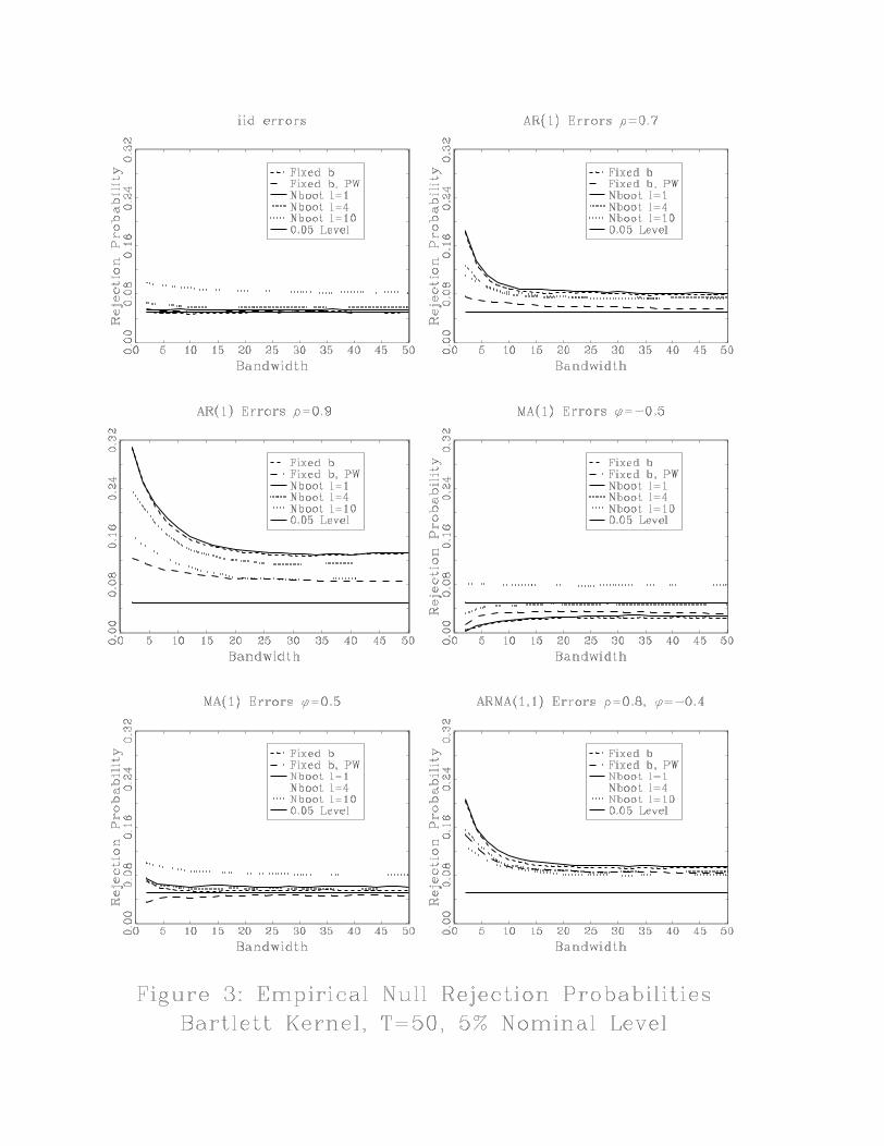
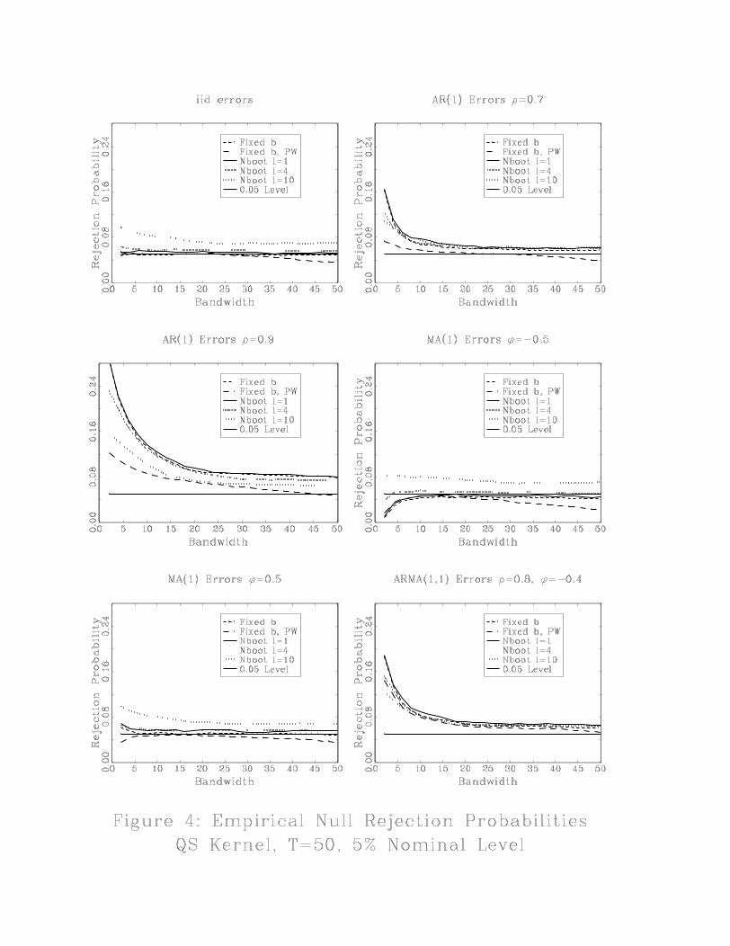
ϕ = −0.5, 0.5 and ARMA(1,1) errors with ρ = 0.8,ϕ = −0.4. We also give results where bΩ isimplemented with AR(1) prewhitening. We report results for the popular Bartlett and quadratic

spectral (QS) kernels. Results for other kernels are similar.

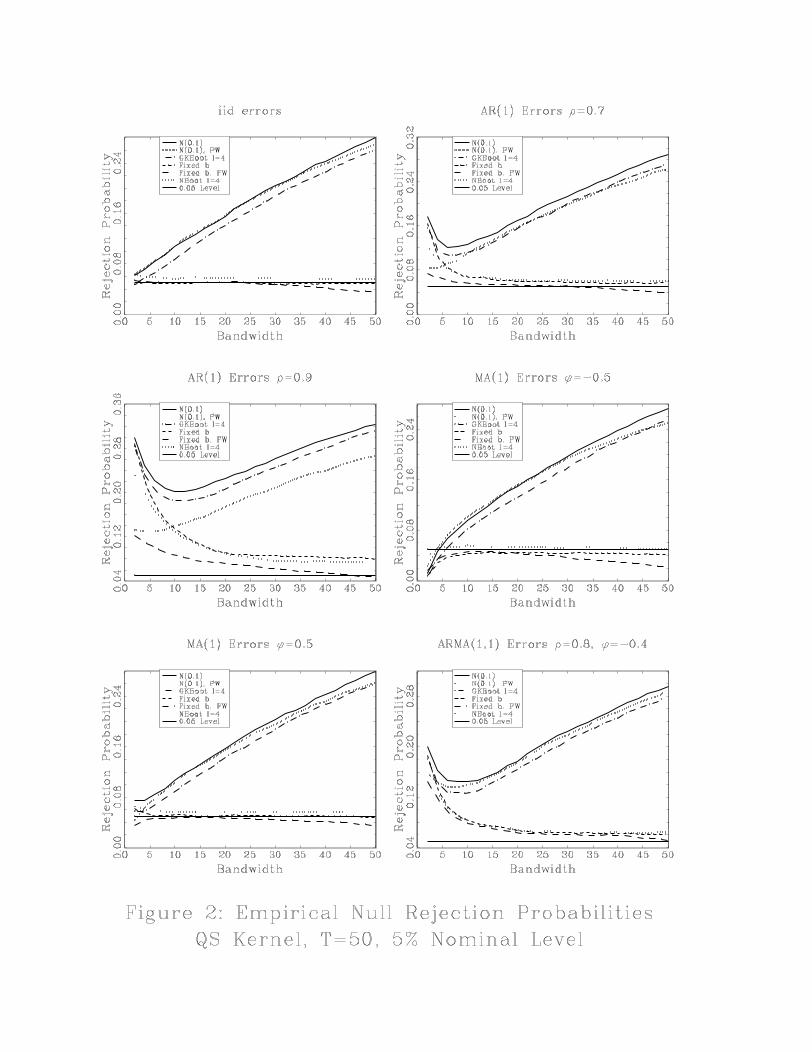
The results are depicted in Figures 1 and 2. In each figure, the line with the label, N(0,1), plots

rejection probabilities when the critical value 1.96 is used and there is no prewhitening. In the case

of prewhitening, the label is N(0,1), PW. The figures also depict plots of rejection probabilities

using the fixed−b asymptotic critical values but for now we only focus on the results using the

standard small-b asymptotics.

Consider first the case of iid errors. When M is small rejection probabilities are only slightly

above 0.05 as one might expect for iid data. However, as M increases, rejection probabilities

steadily rise. WhenM = T, rejection probabilities are nearly 0.2 for the Bartlett kernel and exceed

0.25 for the QS kernel. Similar, although different, patterns occur for AR(1) errors. When M is

8

small, there are nontrivial over-rejection problems. When prewhitening is not used, the rejections

fall asM increases but then rise again asM increases further. When prewhitening is used, rejection

probabilities essential increase as M increases. Prewhitening reduces the extent of over-rejection

but not remove it. The patterns for MA(1) errors are similar to the iid case and the patterns for

ARMA(1,1) errors are combination of the AR(1) and MA(1) cases.

These plots clearly illustrate a fundamental finite sample property of HAC robust tests: the

choice ofM in a given sample matters and can greatly affect the extent of size distortion depending

on the serial correlation structure of the data. And, when M is not very small, the choice of

kernel also matters for the over-rejection problem. Given that the sampling distribution of the

test depends on the bandwidth and kernel, it would seem to be a minimal requirement that the

asymptotic approximation reflect this dependence. Whereas the standard small-b asymptotics is too

crude for this purpose, our results in the next section show that the fixed-b asymptotics naturally

captures the dependence on the bandwidth and kernel and captures the dependence in a simple

and elegant manner4.

Before moving on, it is useful to discuss in some detail the reason that rejection probabilities have

the nonmonotonic pattern for AR(1) errors. When M is small, bΩ is biased but has relatively smallvariance. Because the bias is downward, that leads to over-rejection. As M initially increases, bias

falls and variance rises. The bias effect is more important for over-rejection (see Simonoff (1993))

and the extent of over-rejection decreases. According to the conventional, but wrong, wisdom,

the story would be that as M increases further bias continues to fall but variance increases so

much that over-rejections become worse5. This is not what is happening. In fact, as M increases

further, bias eventually starts to increase and variance begins to fall. It is the increase in bias the

leads to the large over-rejections when M is large. The reason that bias increases and variance

shrinks as M gets large is easy to explain. WhenM is large, high weights are being placed on high

order sample autocovariances. In the extreme case where full weight is placed on all of the sample

autocovariances, it is well known that bΩ is identically equal to zero, and this occurs because bΩ is4An alternative approach to the fixed-b asymptotics is to consider higher order asymptotic approximations in the

small-b framework. For example, one could take the Edgeworth expansions from the recent work by Velasco andRobinson (2001) and obtain a second order asymptotic approximation for HAC robust tests that depends on thebandwidth and kernels. While this is a potentially fruitful approach, it is complicated by the need to estimate thesecond derivative of the spectral density. This estimate would introduce additional sampling variability that couldoffset gains in accuracy from using a higher order approximation. In contrast, the fixed-b asymptotic frameworkrequires no additional estimates.

5This common misperception is an unfortunate result of a folk-lore in the econometrics literature that states that“as M increases, bias in bΩ decreases but variance increases.” This folk-lore is quite misleading although the sourceis easy to pinpoint. A careful reader of Priestley (1981) will repeatedly see the phrase “as M increases, bias in bΩdecreases but variance increases”. This phrase is completely correct if, as in Priestley (1981), one is discussing theproperties of spectral density estimators at non-zero frequencies or, in the case of known mean zero data, at the zerofrequency. However, this phrase does not apply to zero frequency estimators computed using demeaned data as is thecase in GMM models. This fact is well known and has been nicely illustrated by Figure 2 in Ng and Perron (1996)where plots of the exact bias and variance of bΩ are given for AR(1) processes.

9

computed using residuals that have a sample average of zero. Obviously, bΩ = 0 it is an estimatorwith large bias and zero variance. Thus, as M increases, bΩ is pushed closer to the full weight case.4 A New Asymptotic Theory

4.1 Distribution of bΩ in the Fixed-b Asymptotic FrameworkWe now develop a distribution theory for bΩ in the fixed-b asymptotic framework. We proceed underthe asymptotic nesting that M = bT where b ∈ (0, 1] is fixed. The limiting distribution of bΩ in thefixed-b asymptotic framework can be written in terms of Qi(b), an i× i random matrix that takes

on one of three forms depending on the second derivative of the kernel. The following definition

gives the forms of Qi(b).

Definition 1 Let the i× i random matrix, Qi(b) be defined as follows. Case (i): if k(x) is twice

continuously differentiable everywhere,

Qi(b) = −Z 1

0

Z 1

0

1

b2k00(r − sb) eBi(r) eBi(s)0drds.

Case (ii): if k(x) is continuous, k(x) = 0 for |x| ≥ 1, and k(x) is twice continuously differentiableeverywhere except for |x| = 1,

Qi(b) = −ZZ

|r−s|<b1

b2k00(r − sb) eBi(r) eBi(s)0drds

+k0−(1)b

Z 1−b

0

³ eBi(r + b) eBi(r)0 + eBi(r) eBi(r + b)0´dr.where k0−(1) = limh−→0 [(k(1)− k(1− h)) /h], i.e. k0−(1) is the derivative of k(x) from the left at

x = 1. Case (iii): if k(x) is the Bartlett kernel (see the formula appendix)

Qi(b) =2

b

Z 1

0

eBi(r) eBi(r)0dr − 1b

Z 1−b

0

³ eBi(r + b) eBi(r)0 + eBi(r) eBi(r + b)0´dr.The moments of Qi(1) have been derived by Phillips, Sun and Jin (2003) for the case of positive

definite kernels. Hashimzade, Kiefer and Vogelsang (2003) have generalized those results for Qi(b)

while also relaxing the positive definite requirement. The moments are

E (Qi(b)) = Ii

µ1−

ZZk

µr − sb

¶drds

¶,

var (vec (Qi(b))) = ν(b) (Ii2 + κii) ,

ν(b) =

·ZZk

µr − sb

¶drds

¸2− 2

ZZZk

µr − sb

¶k

µr − qb

¶drdsdq +

ZZk

µr − sb

¶2drds,

10

where κii is the standard commutation matrix6 and the range of all integrals is 0 to 1. Using these

moment results, Hashimzade et al. (2003) prove that limb→0E (Qi(b)) = Ii and limb→0 var (vec (Qi(b))) =0. As an illustrative example, consider the Bartlett kernel where

E (Qi(b)) = Ii

µ1− b+ 1

3b2¶,

ν(b) =2

3b− 7

6b2 +

7

15b3 +

1

9b4 for b ≤ 1

2.

We first consider the asymptotic distribution of bΩ for the case of exactly identified models.Theorem 1 (Exactly Identified Models) Suppose that q = p. Let M = bT where b ∈ (0, 1] is fixed.Let Qp(b) be given by Definition 1 for i = p. Then, under Assumptions 1-4, as T →∞,

bΩ⇒ ΛQp(b)Λ0.Several useful observations can be made regarding this theorem. Under fixed-b asymptotics, bΩconverges to a matrix of random variables (rather than constants) that is proportional to Ω through

Λ and Λ0. This contrasts with the small-b asymptotic approximation where bΩ is approximated bythe constant Ω. As b→ 0, it follows from Lemma 1 that p limb→0ΛQp(b)Λ0 = Ω. Thus, the fixed-basymptotics coincides with the standard small-b asymptotics as b goes to zero. The advantage of

the fixed-b asymptotic result is that limit of bΩ depends on the kernel through k00(x) and k0−(1) andon the bandwidth through b but are otherwise nuisance parameter free. Therefore, it is possible to

obtain a first order asymptotic distribution theory that explicitly captures the choice of kernel and

bandwidth. Under fixed-b asymptotics, any choice of bandwidth leads to asymptotically pivotal

tests of hypotheses regarding θ0 when using bΩ to construct standard errors (details are given below).Note that Theorem 1 generalizes results obtained by Kiefer and Vogelsang (2002)a and Kiefer and

Vogelsang (2002)b where the focus was b = 1.

When q > p and the model is overidentified, the limiting expressions for bΩ are more complicatedand asymptotic proportionality to Ω no longer holds. This was established for the special case of

b = 1 by Vogelsang (2000). This does not mean, however, that valid testing is not possible

when using bΩ in overidentified models because the required asymptotic proportionality does holdfor GT (bθT )0WT

bΩWTGT (bθT ), the middle term in bV . The following theorem provides the relevant

result.

Theorem 2 (Over-identified Models) Suppose that q > p. Let M = bT where b ∈ (0, 1] is fixed.Let Qp(b) be given by Definition 1 for i = p. Define Λ∗ = G00W∞Λ. Under Assumptions 1-4, as

6The standard notation for the commutation matrix is usually Kii (see Magnus and Neudecker (1999, p.46). Weare using alternative notation because Kij is used for a different matrix in our proofs.

11

T →∞,

GT (bθT )0WTbΩWTGT (bθT )⇒ Λ∗Qp(b)Λ∗0.

This theorem shows that GT (bθT )0WTbΩWTGT (bθT ) is asymptotically proportional to Λ∗Λ∗0 and

otherwise only depends on the random matrix Qp(b). It directly follows that bV is asymptotically

proportional to V , and asymptotically pivotal tests can be obtained.

4.2 Inference

We now examine the limiting null distributions of tests regarding θ0 under fixed-b asymptotics.

Consider the hypotheses

H0 : r(θ0) = 0

H1 : r(θ0) 6= 0

where r(θ) is an m× 1 vector (m ≤ p) of continuously differentiable functions with first derivativematrix, R(θ) = ∂r(θ)/∂θ0. Applying the delta method to Lemma 1 we obtain

T 1/2r(bθT )⇒ −R(θ0)V 1/2Bp(1) ≡ N(0, VR), (8)

where VR = R(θ0)V R(θ0)0. Using (8) one can construct the standard HAC robust Wald test of thenull hypothesis or a t-test in the case of m = 1. To remain consistent with earlier work, we consider

the F-test version of the Wald statistic defined as

F = Tr(bθT )0 ³R(bθT )bV R(bθT )0´−1 r(bθT )/m,When m = 1 the usual t-statistic can be computed as

t =T 1/2r(bθT )q

R(bθT )bVM=bTR(bθT )0 .Often, the significance of individual statistics are of interest which leads to t-statistics of the form

t =bθiT

se(bθiT ) ,where se(bθi) = p

T−1 bV ii and bV ii is the ith diagonal element of the bV matrix. To avoid any

confusion, please note that these statistics are being computed in exactly the same way as under

the standard approach. Only the asymptotic approximation to the sampling distribution is different.

Note that some kernels, including the Tukey-Hanning, allow negative variance estimates. In this

case some convention must be adopted in calculating the denominator of the test statistics. Equally

12

arbitrary conventions include reflection of negative values through the origin or setting negatives to

a small positive value. Although our results apply to kernels that are not positive definite, we see

no merit in using a kernel allowing negative estimated variances absent a compelling argument in

a specific case. Nevertheless, we have experimented with the Tukey-Hanning and trapezoid kernels

and results not reported here do not support their consideration over a kernel guaranteeing positive

variance estimates.

The following theorem provides the asymptotic null distributions of F and t.

Theorem 3 Let b ∈ (0, 1] be a constant and suppose M = bT . Let Qi(b) be given by Definition 1

for i = m. Then, under Assumptions 1-4 and H0, as T →∞,

F ⇒ Bm(1)0Qm(b)−1Bm(1)/m,

t⇒ B1(1)pQ1(b)

.

Theorem 3 shows that under fixed-b asymptotics, asymptotically pivotal tests are obtained and the

asymptotic distributions reflect the choices of kernel and bandwidth. This contrasts asymptotic

results under the standard approach where F would have a limiting χ2m/m distribution and t a

limiting N(0, 1) distribution regardless of the choice ofM and k(x). It is natural to expect that the

fixed-b asymptotics provide a more accurate approximation in finite samples than the traditional

asymptotics. As shown by the corollary to Theorem 2, as b→ 0, p limQm(b) = Im and the fixed-b

asymptotics reduces to the standard small-b asymptotics. Therefore, if a traditional bandwidth rule

is used in conjunction with the fixed-b asymptotics, in large samples the two asymptotic theories

will coincide. However, because the value of b is strictly greater than zero in practice, it is natural

to expect the fixed-b asymptotics to deliver a more accurate approximation. The simulations results

reported in Section 5 and in the working paper, Kiefer and Vogelsang (2002)c, indicate that this is

true in some simple Gaussian models.

A theoretical comparison of the accuracy of the fixed-b asymptotics with the small-b asymptotics

is not currently available because existing methods in higher order asymptotic expansions, such as

Edgeworth expansions, do not directly apply to the fixed-b asymptotic nesting because of the

nonstandard nature of the distribution theory. Obtaining such theoretical results appears very

difficult although it may be possible to obtain bounds on the rates at which the error in rejection

probability shrinks using the lines of argument in Jansson (2002). Jansson (2002) showed that for

a Gaussian location model the error in rejection probability of F is O(T−1) when M = T (b = 1)

and the Bartlett kernel is used. While it remains an open question whether this results holds more

generally, our simulations are consistent with this possibility. Obviously, this is an area of current

research.

13

4.3 Asymptotic Critical Values

The limiting distributions given by Theorem 3 are nonstandard. Analytical forms of the densities

are not available with the exception of t for the case of the Bartlett kernel with b = 1 (see Abadir and

Paruolo, 2002 and Kiefer and Vogelsang, 2002b). However, because the limiting distributions are

simple functions of standard Brownian motions, critical values are easily obtained using simulations.

In the working paper we provide critical values for the t statistic for a selection of popular kernels

(see the formula appendix for formulas for the kernels). Additional critical values for the F test

will be made available in a follow-up paper.

To make the use of the fixed-b asymptotics easy for practitioners we provide critical value

functions for the t statistic using the cubic equation

cv(b) = a0 + a1b+ a2b2 + a3b

3.

For a selection of well known kernels, we computed the cv(b) function for the percentage points

90%, 95%, 97.5% and 99%. Critical values for the left tail follow by symmetry around zero.

The ai coefficients are given in Table 1. They were obtained as follows. For each kernel and

the grid b = 0.02, 0.04, ...0.98, 1.0 critical values were calculated via simulation methods using

50,000 replications. Normalized partial sums of 1,000 i.i.d. N(0, 1) random deviates were used to

approximate the standard Brownian motions in the respective distributions given by Theorem 3.

For each percentage point, the simulated critical values were used to fit the cv(b) function by OLS.

The intercept was constrained to yield the standard normal critical value so that cv(0) coincides

with the standard asymptotics. Table 1 also reports the R2 from the regressions and the fits are

excellent in all cases (R2 ranging from 0.9825 to 0.9996).

5 Choice of Kernel and Bandwidth: Performance

In this section we analyze the choice of kernel and bandwidth on the performance of HAC robust

tests. We focus on accuracy of the asymptotic approximation under the null and on local asymptotic

power. As far as we know, our analysis is the first to explore theoretically the effects of kernel and

bandwidth choice on power of HAC robust tests.

5.1 Accuracy of the Asymptotic Approximation under the Null and Comparison withthe Bootstrap

The way to evaluate the accuracy of an asymptotic approximation to a null distribution, or indeed

any approximation, is to compare the approximate distribution to the exact distribution. Sometimes

this can be done analytically; more commonly the comparison can be made by simulation. We

argued above that our approximation to the distribution of HAC robust tests was likely to be

14

better than the usual approximation, since ours takes into account the randomness in the estimated

variance. However, as noted, that argument is unconvincing in the absence of evidence on the

approximation’s performance. We provide results for two popular positive definite kernels: Bartlett

and QS. Results for the Parzen, Bohman and Daniell kernel are similar and are not reported here.

The working paper, Kiefer and Vogelsang (2002)c, contains additional finite sample simulation

results that are similar to what is reported here.

The simulations were based on the simple location model (7) with same design as described

previously. Figures 1 and 2 provide plots of empirical rejection probabilities using the fixed-b

asymptotics. Compared to the standard small-b asymptotics, the results are striking. In nearly all

cases, the tendency to over-reject is substantially reduced. The exceptions are for small values ofM

where the fixed-b asymptotics show only small improvements. But, this is to be expected given that

the two asymptotic theories coincide as b goes to 0. In the case of MA errors, fixed-b asymptotics

gives tests with rejection probabilities close to 0.05. In the case of AR errors, over-rejections

decrease as M increases. This pattern is consistent with Hashimzade and Vogelsang (2003) who

found in finite sample simulations that the fixed-b asymptotic approximation for bΩ improves asM increases. Intuitively, the fixed-b asymptotics is capturing the downward bias in bΩ that can besubstantial when M is large. As M increases, the tendency to over-reject falls. The QS kernel

delivers tests with less size distortions than the Bartlett kernel especially when M is large.

The results in Figures 1 and 2 strongly suggest that the use of fixed-b asymptotic critical values

greatly improves the performance of HAC robust t-tests.

The improvement of the asymptotic approximation using fixed-b asymptotics occurs because

fixed-b asymptotics captures much of the bias and sampling variability induced by the kernel and

bandwidth. In the case of iid errors, the fixed-b asymptotics is remarkably accurate. As serial

correlation in the errors becomes stronger, the tendency to over-reject appears. The reason is

that the functional central limit theorem approximation begins to erode. Therefore, there may be

potential for the bootstrap to provide further refinements in accuracy. The fixed-b asymptotics

suggests that the bootstrap could work because the HAC robust tests are asymptotically pivotal

for any kernel and bandwidth.

Ideally, one would like to establish theoretically whether or not the bootstrap provides an

asymptotic refinement. Such a theoretical exercise is well beyond the scope of this paper because

higher order expansions for fixed-b asymptotics have not been developed. Obtaining such expansions

is an important topic that deserves attention.

To show the potential of the bootstrap for HAC robust tests, we expanded our simulation

study to include the block bootstrap. We implemented the block bootstrap following Gotze and

Kunsch (1996) as follows. The original data, y1, y2, ..., yT is divided into T − l + 1 overlappingblocks of length, l. For simplicity, we report results for l = 1, 4, 10 all of which factor into T = 50.

15

T/l blocks are drawn randomly with replacement to form a bootstrap sample labeled y∗1, y∗2, ..., y∗T .The bootstrap t statistic is computed in two ways. The first statistic, labelled the naive bootstrap

test, is defined as

t∗Naive =√T (bµ∗ − y)pbΩ∗ ,

where bµ∗ = y∗ = T−1PTt=1 y

∗t and bΩ∗ is computed using formula (6) with f(y∗t , bµ∗) = bu∗t = y∗t − bµ∗.

The second statistic, labelled the Gotze-Kunsch (GK) bootstrap test, is defined as

t∗GK =√T¡bµ∗ − y¢peΩ∗ , where

y = (T − l + 1)−1T−lXj=0

Ãl−1

lXi=1

yj+i

!, eΩ∗ = T−1 T/lX

j=1

ÃlXi=1

bu∗l∗(j−1)+i!2.

The centering and standardization of the GK test is required for the bootstrap to attain second

order accuracy under small-b asymptotics.

Empirical rejection probabilities using the bootstrap critical values are reported in Figures 1,

2, 3 and 4. The label NBoot refers to the naive bootstrap and the label GKBoot refers to the GK

bootstrap. In Figures 1 and 2 the block length is 4. In figures 3 and 4 results are reported for the

naive bootstrap for block lengths 1, 4 and 10.

There are some very compelling patterns in the Figures. In figures 1 and 2 it is obvious that the

GK bootstrap provides a more accurate approximation than the standard normal approximation

although for AR(1) errors the prewhitened standard normal approximation outperforms the GK

bootstrap. On the other hand, the GK bootstrap is inferior to the fixed-b asymptotic approximation

except when b is very close to zero (M = 1, 2) in which case differences are small. These simulation

results suggest that while the GK bootstrap provides the expected asymptotic refinement over

the standard normal approximation, it does not approach the accuracy of the fixed-b asymptotics

when M is not very small. This is not that surprising given that the theoretical results for the

GK bootstrap were obtained under the small-b asymptotic nesting. It is well known that the GK

bootstrap does not attain second order correctness when the Bartlett kernel is used. Yet, the

simulations suggest that GK bootstrap appears to provide refinements when the Bartlett kernel is

used.

Contrary to theoretical results by Davison and Hall (1993) in the bootstrap literature, the naive

bootstrap performs quite well and yields rejection probabilities that are very similar to the fixed-b

asymptotics. It appears that the naive bootstrap may provide a higher order refinement over the

fixed-b asymptotics although in the case of AR(1) errors, prewhitening and fixed-b asymptotics is

more accurate than the naive bootstrap.

16

Regardless of the data generating process or kernel, it is striking how the naive bootstrap closely

follows the fixed-b asymptotics while the GK bootstrap closely follows the standard small-b asymp-

totics. Clearly, there are some very interesting properties of the bootstrap that warrant additional

research. It appears that fixed-b asymptotics could play an important role in understanding the

strong performance of the naive bootstrap in spite of the negative theoretical results obtained in

the literature. Our conjecture is that while the GK bootstrap nails the second order term of the

small-b Edgeworth expansion, the Edgeworth expansion itself does not provide a very accurate

approximation when the bandwidth isn’t small. On the other hand, we conjecture that the naive

bootstrap may capture a second order term in the fixed-b asymptotics. We hope these interesting

puzzles will stimulate new theoretical work in the bootstrap literature.

Finally, we report some results in Figures 3 and 4 illustrating the sensitivity of the naive

bootstrap to the choice of block length. For AR(1) processes, a block length of 10 does fairly well,

almost as well as the prewhitened test with fixed-b critical values. In contrast for MA(1) errors, a

large block length can cause the bootstrap to perform more poorly than the fixed-b asymptotics.

6 Local Asymptotic Power

Whereas the existing HAC literature has almost exclusively focused on the MSE of the HAC

estimator to guide the choice of kernel and bandwidth, a more relevant metric is to focus on the

power of the resulting tests. In this section we compare power of HAC robust t-tests using a

local asymptotic power analysis within the fixed-b asymptotic framework. Our analysis permits

comparison of power across bandwidths and across kernels. Such a comparison is not possible

using the traditional first order small-b asymptotics because local asymptotic power is the same for

all bandwidths and kernels.

For clarity, we restrict attention to linear regression models. Given the results in Theorem 1,

the derivations in this section are very simple extensions of results given by Kiefer and Vogelsang

(2002)a. Therefore, details are kept to a minimum. Consider the regression model

yt = x0tθ0 + ut (9)

with θ0 and xt p × 1 vectors. In terms of the general model we have f(vt, θ0) = xt (yt − x0tθ0).Without loss of generality, we focus on θi0, one element of θ, and consider null and alternative

hypotheses

H0 : θi0 ≤ 0H1 : θi0 = cT

−1/2

where c > 0 is a constant. If the regression model satisfies Assumptions 1 through 4, then we can

use the results of Theorem 1 and results from Kiefer and Vogelsang (2002)a to easily establish that

17

under the local alternative, H1, as T →∞,

t∗b ⇒δ +B1(1)pQ1(b)

, (10)

where δ = c/√V ii, V ii is the ith diagonal element of V, and Q1(b) is given by Definition 1 for i = 1.

Asymptotic power curves can be computed for given bandwidths and kernels by simulating the

asymptotic distribution of t∗b based on (10) for a range of values for δ and computing rejectionprobabilities with respect to the relevant null critical value. Using the same simulation methods as

for the asymptotic critical values, local asymptotic power was computed for δ = 0, 0.2, 0.4, ..., 4.8, 5.0

using 5% asymptotic null critical values.

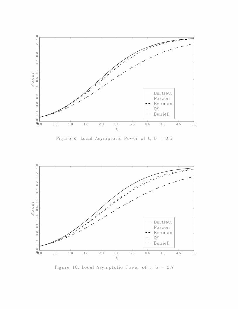
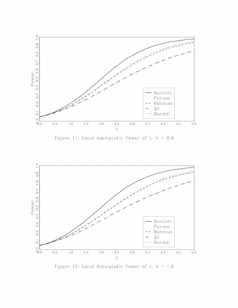
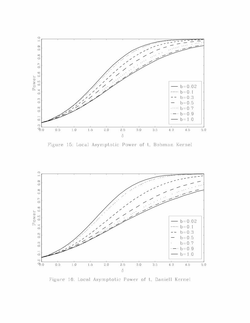
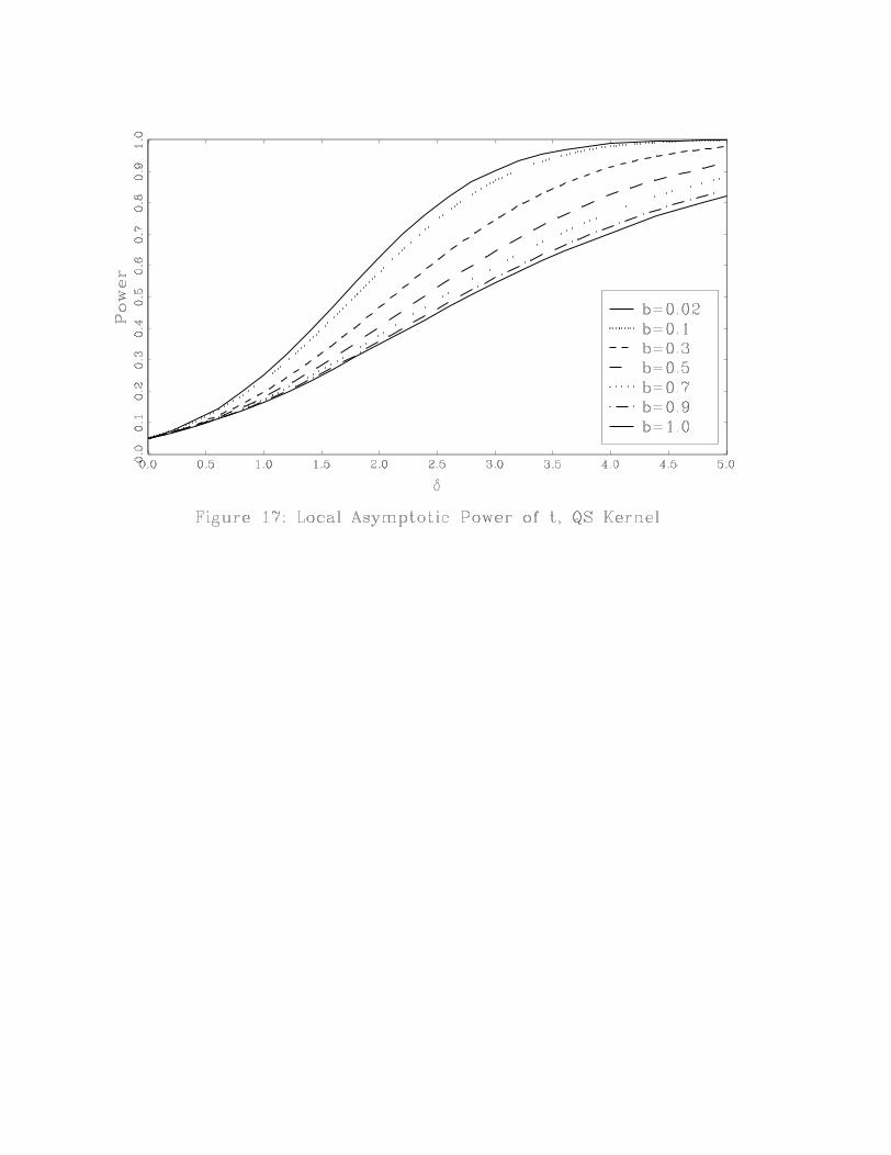
The power results are reported in two ways. Figures 5-12 plot power across the kernels for a

given value of b. Figures 13-17 plot power across values of b for a given kernel. Figures 5-12 show

that for small bandwidths, power is essentially the same across kernels. As b increases, it becomes

clear that the Bartlett kernel has the highest power while the QS and Daniell kernels have the

lowest power. If power is the criterion used to choose a test, then the Bartlett kernel is the best

choice within this set of five kernels. If we compare the Bartlett and QS kernels, we see that the

power ranking of these kernels is the reverse of their ranking based on accuracy of the asymptotic

approximation under the null.

Figures 13-17 show how the choice of bandwidth affects power. Regardless of the kernel, power

is highest for small bandwidths and lowest for large bandwidths and power is decreasing in b. These

figures also show that power of the Bartlett kernel is least sensitive to b whereas power of the

QS and Daniell kernels is the most sensitive to b. Again, power rankings of b are the opposite of

rankings of b based on accuracy of the asymptotic approximation under the null.

7 Conclusions

We have provided a new approach to the asymptotic theory of HAC robust testing. We consider

tests based on the popular kernel based nonparametric estimates of the standard errors. We are not

proposing new tests but rather we propose a new asymptotic theory for these well known tests. Our

results are general enough to apply to stationary models estimated by GMM. In our approach, b,

the ratio of bandwidth to sample size is held constant when deriving the asymptotic behavior of the

relevant covariance matrix estimator (i.e. zero frequency spectral density estimator). Thus we label

our asymptotic framework “fixed-b” asymptotics. In standard asymptotics, b is sent to zero and

can be viewed as a “small-b” asymptotic framework. Fixed-b asymptotics improves upon two well

known problems with the standard approach. First, as has been well documented in the literature,

the standard asymptotic approximation of the sampling behavior of tests is often poor. Second, the

kernel and bandwidth choice do not appear in the approximate distribution, leaving the standard

18

theory silent on the choice of kernel and bandwidth with respect to properties of the tests. Our

theory leads to approximate distributions that explicitly depend on the kernel and bandwidth. The

new approximation performs much better and gives insight into the choice of kernel and bandwidth

with respect to test behavior. Fixed-b asymptotics should be useful in explaining the performance

of the naive bootstrap when applied to HAC robust tests.

The new approximations should be used for HAC robust test statistics for any choice of kernel

and bandwidth. Our approximation is an unambiguous improvement over the standard approxi-

mation in most cases considered. We show that size distortions are reduced when large bandwidths

are used, but so is asymptotic power. Generally there is a trade-off in bandwidth and kernel choice

between size (the accuracy of the approximation) and power. Among a group of popular kernels,

the QS kernel leads to the least size distortion, while the Bartlett kernel leads to tests with highest

power (and generally acceptable size distortion when large bandwidths are used).

8 Appendix: Proofs

We first define some relevant functions and derive preliminary results before proving the lemma

and theorems. Define the functions

k∗ (x) = k³xb

´,

Kij = k

µi− jbT

¶= k∗

µi− jT

¶,

∆2Kij = (Kij −Ki,j+1)− (Ki+1,j −Ki+1,j+1) ,

D∗T (r) = T2

·µk∗µ[rT ] + 1

T

¶− k∗

µ[rT ]

T

¶¶−µk∗µ[rT ]

T

¶− k∗

µ[rT ]− 1T

¶¶¸.

Notice that

T 2∆2Kij = −D∗Tµi− jT

¶.

Because k(r) is an even function around r = 0,D∗T (−r) = D∗T (r). If k∗00(r) exists then limT→∞D∗T (r) =k∗00(r) by the definition of the second derivative. If k∗00(r) is continuous, then D∗T (r) converges tok∗00(r) uniformly in r. Define the stochastic process

XT (r) = GT (bθT )0WTT1/2g[rT ](θ0).

It directly follows from Assumptions 2, 3 and 4 that

XT (r)⇒ G00W∞ΛBq(r) ≡ Λ∗Bp(r). (11)

19

Proof of Lemma 1: Setting t = T , multiplying both sides of (4) by GT (bθT )0WT , and using the

first order condition GT (bθT )0WT gT (bθT ) = 0 gives0 = GT (bθT )0WT gT (θ0) +GT (bθT )0WTGT (bθT , θ0,λT )(bθT − θ0). (12)

Solving (12) for (bθT − θ0) and scaling by T 1/2 gives

T 1/2(bθT − θ0) = −[G0T (bθT )WTGT (bθT , θ0,λT )]−1G0T (bθT )WTT1/2gT (θ0)

= −[GT (bθT )0WTGT (bθT , θ0,λT )]−1XT (1). (13)

Because p limGT (bθT )0WTGT (bθT , θ0,λT ) = G00W∞G0 by Assumptions 3 and 4, it follows from (11)

that

T 1/2(bθT − θ0)⇒ −¡G00W∞G0

¢−1Λ∗Bp(r).

The proof of Theorem 1 follows the same arguments as the proof for Theorem 2 and is omitted.

Proof of Theorem 2: Define the random process

eXT (r) = GT (bθT )0WTT1/2g[rT ](bθT ).

Plugging in for g[rT ](bθT ) using (4) giveseXT (r) = XT (r) +GT (bθT )0WTG[rT ](bθT , θ0,λT )T 1/2(bθT − θ0)

= XT (r)−GT (bθT )0WTG[rT ](bθT , θ0,λT ) hGT (bθT )0WTGT (bθT , θ0,λT )i−1XT (1),using (13). It directly follows from Assumptions 3 and 4 and (11) that

eXT (r)⇒ Λ∗Bp(r)− rG00W∞G0 ¡G00W∞G0¢−1 Λ∗Bp(1)= Λ∗ (Bp(r)− rBp(1)) ≡ Λ∗ eBp(r). (14)

Straightforward algebra gives

bΩ = T−1Xj=−(T−1)

k

µj

bT

¶ bΓj = T−1 TXi=1

TXj=1

f(vi, bθT )Kijf(vj , bθT )0.Using algebraic arguments similar to those used by Kiefer and Vogelsang (2002)a, it is straightfor-

ward to show that

bΩ = T−1 T−1Xi=1

T−1Xj=1

∆2KijTgi(bθT )Tgj(bθT )0+ gT (bθT ) T−1X

i=1

(KTi −KT,i+1)Tgi(bθT )0 + TXj=1

f(vj , bθT )KjT gT (bθT )0. (15)

20

Using (15) it directly follows that

GT (bθT )0WTbΩWTGT (bθT )

= T−1T−1Xi=1

T−1Xj=1

∆2KijGT (bθT )0WTTgi(bθT )Tgj(bθT )0WTGT (bθT )= T−2

T−1Xi=1

T−1Xj=1

T 2∆2KijGT (bθT )0WTT1/2gi(bθT )T 1/2gj(bθT )0WTGT (bθT )

= T−2T−1Xi=1

T−1Xj=1

−D∗Tµi− jT

¶GT (bθT )0WTT

1/2gi(bθT )T 1/2gj(bθT )0WTGT (bθT ) (16)

where the second and third terms of (15) vanish because from (3) we have

GT (bθT )0WTTgT (bθT ) = 0,TgT (bθT )0WTGT (bθT ) = 0.

The rest of proof is divided into three cases.

Case 1: k(x) is twice continuously differentiable. Using (16) it follows that

GT (bθT )0WTbΩWTGT (bθT )

= −Z 1

0

Z 1

0D∗T (r − s)GT (bθT )0WTT

1/2g[rT ](bθT )T 1/2g[sT ](bθT )0WTGT (bθT )drds= −

Z 1

0

Z 1

0D∗T (r − s) eXT (r) eXT (s)0drds

⇒−Λ∗Z 1

0

Z 1

0k∗00(r − s) eBp(r) eBp(s)0drdsΛ∗0,

using the continuous mapping theorem. The final expression is obtained using k∗00(x) = 1b2k

00(xb ).

Case 2: k(x) is continuous, k(x) = 0 for |x| ≥ 1, and k(x) is twice continuously differentiable

everywhere except for |x| = 1. Let 1(•) denote the indicator function. Noting that ∆2Kij = 0 for|i− j| > [bT ] and ∆2Kij = −k∗

¡b− 1

T

¢for |i− j| = [bT ], break up the double sum in the second

line of the expression for GT (bθT )0WTbΩWTGT (bθT ) into three pieces corresponding to |i− j| < [bT ],

|i− j| = [bT ], and |i− j| > [bT ] to obtain

GT (bθT )0WTbΩWTGT (bθT ) =

21

T−2T−1Xi=1

T−1Xj=1

1 (|i− j| < [bT ])T 2∆2KijGT (bθT )0WTT1/2gi(bθT )T 1/2gj(bθT )0WTGT (bθT )

− Tk∗µb− 1

T

¶T−1

T−[bT ]−1Xi=1

GT (bθT )0WTT1/2gi+[bT ](bθT )T 1/2gi(bθT )0WTGT (bθT )

− Tk∗µb− 1

T

¶T−1

T−[bT ]−1Xj=1

GT (bθT )0WTT1/2gj(bθT )T 1/2gj+[bT ](bθT )0WTGT (bθT ).

It directly follows that

GT (bθT )0WTbΩWTGT (bθT ) =

−ZZ

|r−s|<bD∗T (r − s) eXT (r) eXT (s)0drds− Tk∗µb− 1

T

¶Z 1−b

0

³ eXT (r + b) eXT (r)0 + eXT (r) eXT (r + b)0´dr.Let k∗0_(b) denote the first derivative of k∗(x) from the left at x = b. By definition

k0−(1)b

= k∗0_(b) = limT→∞

·−Tk∗

µb− 1

T

¶¸.

Therefore, by the continuous mapping theorem

GT (bθT )0WTbΩWTGT (bθT )dr⇒

Λ∗"−ZZ

|r−s|<bk∗00(r − s) eBp(r) eBp(s)0drds+ k∗0_(b)Z 1−b

0

³ eBp(r + b) eBp(r)0 + eBp(r) eBp(r + b)0´dr#Λ∗0.Case 3: k(x) is the Bartlett kernel. It is easy to calculate that for the Bartlett kernel, ∆2Kij = 2

bT

for |i− j| = 0, ∆2Kij = − 1bT for |i− j| = [bT ] and ∆2Kij = 0 otherwise. Therefore we have

GT (bθT )0WTbΩWTGT (bθT ) =

2

bT

T−1Xi=1

GT (bθT )0WTT1/2gi(bθT )T 1/2gi(bθT )0WTGT (bθT )

− 1

bT

T−[bT ]−1Xi=1

GT (bθT )0WTT1/2gi+[bT ](bθT )T 1/2gi(bθT )0WTGT (bθT )

− 1

bT

T−[bT ]−1Xj=1

GT (bθT )0WTT1/2gj(bθT )T 1/2gj+[bT ](bθT )0WTGT (bθT )

22

=2

b

Z 1

0

eXT (r) eXT (r)0dr − 1b

Z 1−b

0

³ eXT (r + b) eXT (r)0 + eXT (r) eXT (r + b)0´dr⇒ Λ∗

·2

b

Z 1

0

eBp(r) eBp(r)0dr − 1b

Z 1−b

0

³ eBp(r + b) eBp(r)0 + eBp(r) eBp(r + b)0´dr¸Λ∗0.Proof of Theorem 3: We only give the proof for F ∗ as the proof for t∗ follows using similararguments. Applying the delta method to the result in Lemma 1 and using the fact that Bq(1) is

a vector of independent standard normal random variables gives

T 1/2r(bθT )⇒−R(θ0) ¡G00W∞G0¢−1G00W∞ΛBq(1)≡ −R(θ0)

¡G00W∞G0

¢−1Λ∗Bp(1)

≡ Λ∗∗Bm(1), (17)

where Λ∗∗ is the matrix square root of R(θ0) (G00W∞G0)−1 Λ∗Λ∗0 (G00W∞G0)

−1R(θ0)0. Using theresults in Theorem 2, it directly follows that

R(bθT )bVM=bTR(bθT )0 = R(bθT ) hGT (bθT )0WTGT (bθT , θ0,λT )i−1GT (bθT )0WTbΩM=TWTGT (bθT )

×hGT (bθT )0WTGT (bθT , θ0,λT )i−1R(bθT )0

⇒ R(θ0)¡G00W∞G0

¢−1Λ∗Qp(b)Λ∗0

¡G00W∞G0

¢−1R(θ0)

0

≡ Λ∗∗Qm(b)Λ∗∗0, (18)

where we use the fact that

R(θ0)¡G00W∞G0

¢−1Λ∗ eBp(r) = R(θ0) ¡G00W∞G0¢−1Λ∗ (Bp(r)− rBp(1))

≡ Λ∗∗ (Bm(r)− rBm(1))= Λ∗∗ eBm(r).

Using (17) and (18) it directly follows that

F ∗ = Tr(bθT )0 ³R(bθT )bVM=bTR(bθT )0´−1 r(bθT )/m= T 1/2r(bθT )0 ³R(bθT )bVM=TR(bθT )0´−1 T 1/2r(bθT )/m⇒ (Λ∗∗Bm(1))0

¡Λ∗∗Qm(b)Λ∗∗0

¢−1(Λ∗∗Bm(1)) /m

≡ Bm(1)0Qm(b)−1Bm(1)/m,

which completes the proof.

23

9 Appendix: Kernel Formulas

The formulas for the kernels analyzed in this paper are

Bartlett k(x) =

½1− |x| for |x| ≤ 1,0 otherwise,

Parzen k(x) =

1− 6x2 + 6|x|3 for |x| ≤ 1

2 ,2(1− |x|)3 for 1

2 ≤ |x| ≤ 10 otherwise,

Bohman k(x) =

½(1− |x|) cos(πx) + sin(π |x|)/π for |x| ≤ 1,

0 otherwise,

Quadratic Spectral (QS) k(x) =25

12π2x2

µsin(6πx/5)

6πx/5− cos(6πx/5)

¶,

Daniell k(x) =sin(πx)

πx.

24

References

Abadir, K. M. and Paruolo, P. (2002), Simple Robust Testing of Regression Hypotheses: a Com-

ment, Econometrica 70, 2097—2099.

Andrews, D. W. K. (1991), Heteroskedasticity and Autocorrelation Consistent Covariance Matrix

Estimation, Econometrica 59, 817—854.

Andrews, D. W. K. and Monahan, J. C. (1992), An Improved Heteroskedasticity and Autocorrela-

tion Consistent Covariance Matrix Estimator, Econometrica 60, 953—966.

Barndorff-Nielsen, O. and Cox, D. (1989), Asymptotic Techniques for Use in Statistics, Chapman

and Hall, London.

Berk, K. N. (1974), Consistent Autoregressive Spectral Estimates, The Annals of Statistics 2, 489—

502.

Bunzel, H., Kiefer, N. M. and Vogelsang, T. J. (2001), Simple Robust Testing of Hypotheses in

Non-linear Models, Journal of American Statistical Association 96, 1088—1098.

Cushing, M. J. and McGarvey, M. G. (1999), Covariance Matrix Estimation, in L. Matyas (ed.),

Generalized Method of Moments Estimation, Cambridge University Press, New York.

Davison, A. C. and Hall, P. (1993), On Studentizing and Blocking Methods for Implementing the

Bootstrap with Dependent Data, Australian Journal of Statistics 35, 215—224.

de Jong, R. M. and Davidson, J. (2000), Consistency of Kernel Estimators of Heteroskedastic and

Autocorrelated Covariance Matrices, Econometrica 68, 407—424.

den Haan, W. J. and Levin, A. (1997), A Practictioner’s Guide to Robust Covariance Matrix

Estimation, inG. Maddala and C. Rao (eds), Handbook of Statistics: Robust Inference, Volume

15, Elsevier, New York, pp. 291—341.

den Haan, W. J. and Levin, A. (1998), Vector Autoregressive Covariance Matrix Estimation, work-

ing paper, International Finance Division, FED Board of Governors.

Gallant, A. (1987), Nonlinear Statistical Models, Wiley, New York.

Gallant, A. and White, H. (1988), A Unified Theory of Estimation and Inference for Nonlinear

Dynamic Models, Basil Blackwell, New York.

Gotze, F. and Kunsch, H. R. (1996), Second-Order Correctness of the Blockwise Bootstrap for

Stationary Observations, Annals of Statistics 24, 1914—1933.

25

Hall, P. and Horowitz, J. L. (1996), Bootstrap Critical Values for Tests Based on Generalized

Method of Moments Estimators, Econometrica 64, 891—916.

Hansen, B. E. (1992), Consistent Covariance Matrix Estimation for Dependent Heterogenous Pro-

cesses, Econometrica 60, 967—972.

Hansen, L. P. (1982), Large Sample Properties of Generalized Method of Moments Estimators,

Econometrica 50, 1029—1054.

Hashimzade, N. and Vogelsang, T. J. (2003), A New Asymptotic Approximation for the Sampling

Behavior of Spectral Density Estimators, Working Paper, Department of Economics, Cornell

University.

Hashimzade, N., Kiefer, N. M. and Vogelsang, T. J. (2003), Moments of HAC Robust Covariance

Matrix Estimators Under Fixed-b Asymptotics, Working Paper, Department of Economics,

Cornell University.

Heyde, C. (1997), Quasi-Likelihood and its Application. A General Approach to Optimal Parameter

Estimation, Springer, New York.

Inoue, A. and Shintani, M. (2001), Bootstrapping GMM Estimators for Time Series, Working

paper, Department of Agriculture and Resource Economics, NC State.

Jansson, M. (2002), Autocorrelation Robust Tests with Good Size and Power, Working Paper,

Department of Economics, U.C. Berkeley.

Kiefer, N. M. and Vogelsang, T. J. (2002)a, Heteroskedasticity-Autocorrelation Robust Testing

Using Bandwidth Equal to Sample Size, Econometric Theory 18, 1350—1366.

Kiefer, N. M. and Vogelsang, T. J. (2002)b, Heteroskedasticity-Autocorrelation Robust Standard

Errors Using the Bartlett Kernel Without Truncation, Econometrica 70, 2093—2095.

Kiefer, N. M. and Vogelsang, T. J. (2002)c, A New Asymptotic Theory for Heteroskedasiticy-

Autocorrelation Robust Tests, Working Paper, Center for Analytic Economics, Cornell Uni-

versity.

Kiefer, N. M., Vogelsang, T. J. and Bunzel, H. (2000), Simple Robust Testing of Regression Hy-

potheses, Econometrica 68, 695—714.

Magnus, J. R. and Neudecker, H. (1999),Matrix Differential Calculus with Applications in Statistics

and Econometrics, Wiley, New York.

26

Neave, H. R. (1970), An Improved Formula for the Asymptotic Variance of Spectrum Estimates,

Annals of Mathematical Statistics 41, 70—77.

Newey, W. K. and McFadden, D. L. (1994), Large Sample Estimation and Hypothesis Testing,

in R. Engle and D. L. McFadden (eds), Handbook of Econometrics, Vol. 4, Elsevier Science

Publishers, Amseterdam, The Netherlands, pp. 2113—2247.

Newey, W. K. and West, K. D. (1987), A Simple, Positive Semi-Definite, Heteroskedasticity and

Autocorrelation Consistent Covariance Matrix, Econometrica 55, 703—708.

Newey, W. K. and West, K. D. (1994), Automatic Lag Selection in Covariance Estimation, Review

of Economic Studies 61, 631—654.

Ng, S. and Perron, P. (1996), The Exact Error in Estimating the Spectral Density at the Origin,

Journal of Time Series Analysis 17, 379—408.

Phillips, P. C. B. and Durlauf, S. N. (1986), Multiple Regression with Integrated Processes, Review

of Economic Studies 53, 473—496.

Phillips, P. C. B., Sun, Y. and Jin, S. (2003), Consistent HAC Estimation and Robust Regres-

sion Testing Using Sharp Origin Kernels with No Truncation, Working Paper, Department of

Economics, Yale University.

Priestley, M. B. (1981), Spectral Analysis and Time Series, Vol. 1, Academic Press, New York.

Robinson, P. (1998), Inference-Without Smoothing in the Presence of Nonparametric Autocorrela-

tion, Econometrica 66, 1163—1182.

Simonoff, J. (1993), The Relative Importance of Bias and Variability in the Estimation of the

Variance of a Statistic, The Statistician 42, 3—7.

Velasco, C. and Robinson, P. M. (2001), Edgeworth Expansions for Spectral Density Estimates and

Studentized Sample Mean, Econometric Theory 17, 497—539.

Vogelsang, T. J. (2000), Testing in GMM Models Without Truncation, Center for Analytic Eco-

nomics, Working Paper 01-12, Cornell University, forthcoming in Advances in Econometrics

Volume 17.

White, H. (1984), Asymptotic Theory for Econometricians, Academic Press, New York.

27

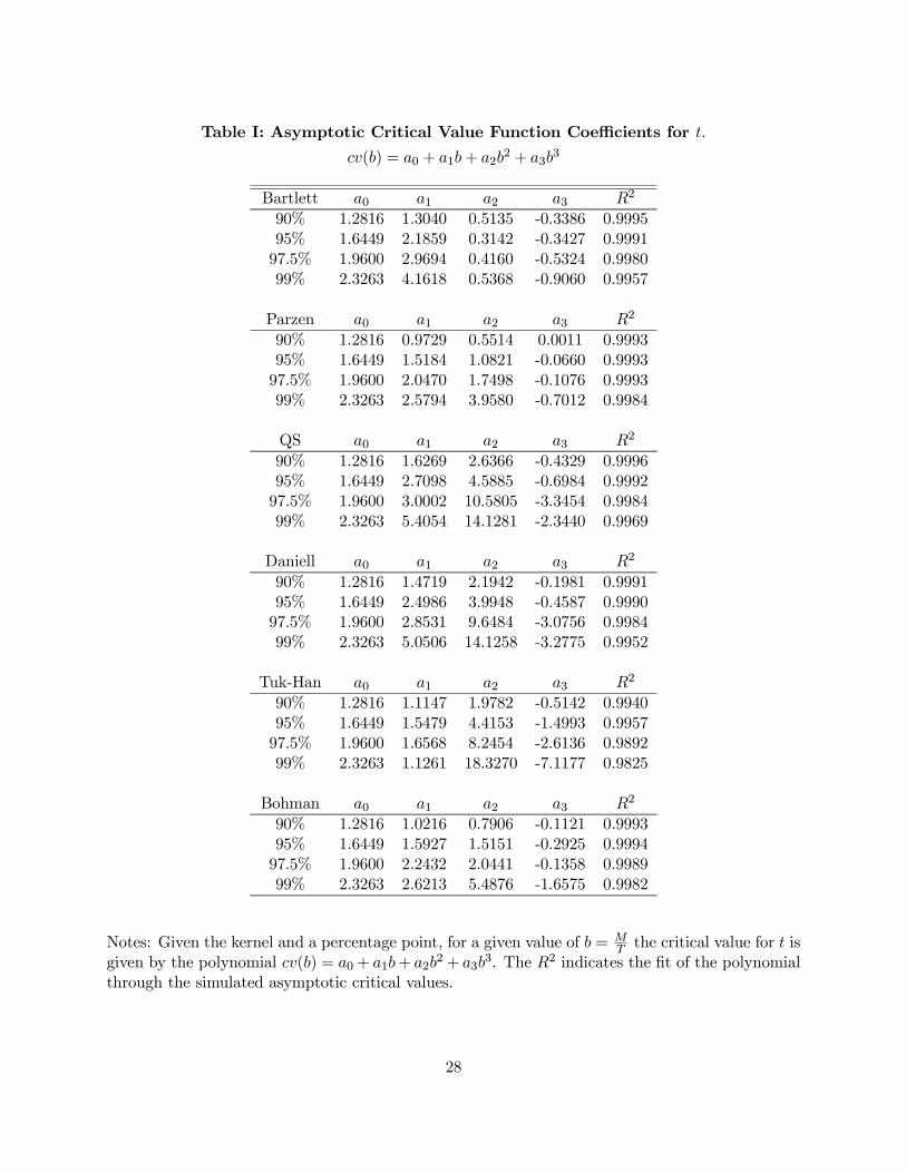
Table I: Asymptotic Critical Value Function Coefficients for t.

cv(b) = a0 + a1b+ a2b2 + a3b

3

Bartlett a0 a1 a2 a3 R2

90% 1.2816 1.3040 0.5135 -0.3386 0.999595% 1.6449 2.1859 0.3142 -0.3427 0.999197.5% 1.9600 2.9694 0.4160 -0.5324 0.998099% 2.3263 4.1618 0.5368 -0.9060 0.9957

Parzen a0 a1 a2 a3 R2

90% 1.2816 0.9729 0.5514 0.0011 0.999395% 1.6449 1.5184 1.0821 -0.0660 0.999397.5% 1.9600 2.0470 1.7498 -0.1076 0.999399% 2.3263 2.5794 3.9580 -0.7012 0.9984

QS a0 a1 a2 a3 R2

90% 1.2816 1.6269 2.6366 -0.4329 0.999695% 1.6449 2.7098 4.5885 -0.6984 0.999297.5% 1.9600 3.0002 10.5805 -3.3454 0.998499% 2.3263 5.4054 14.1281 -2.3440 0.9969

Daniell a0 a1 a2 a3 R2

90% 1.2816 1.4719 2.1942 -0.1981 0.999195% 1.6449 2.4986 3.9948 -0.4587 0.999097.5% 1.9600 2.8531 9.6484 -3.0756 0.998499% 2.3263 5.0506 14.1258 -3.2775 0.9952

Tuk-Han a0 a1 a2 a3 R2

90% 1.2816 1.1147 1.9782 -0.5142 0.994095% 1.6449 1.5479 4.4153 -1.4993 0.995797.5% 1.9600 1.6568 8.2454 -2.6136 0.989299% 2.3263 1.1261 18.3270 -7.1177 0.9825

Bohman a0 a1 a2 a3 R2

90% 1.2816 1.0216 0.7906 -0.1121 0.999395% 1.6449 1.5927 1.5151 -0.2925 0.999497.5% 1.9600 2.2432 2.0441 -0.1358 0.998999% 2.3263 2.6213 5.4876 -1.6575 0.9982

Notes: Given the kernel and a percentage point, for a given value of b = MT the critical value for t is

given by the polynomial cv(b) = a0+ a1b+ a2b2+ a3b3. The R2 indicates the fit of the polynomialthrough the simulated asymptotic critical values.

28