a new equation of state for better liquid density
TRANSCRIPT
The Pennsylvania State University
The Graduate School
College of Energy and Mineral Engineering
A NEW EQUATION OF STATE FOR BETTER LIQUID DENSITY PREDICTION OF
NATURAL GAS SYSTEMS
A Dissertation in Petroleum and Mineral Engineering
by
Princess C. Nwankwo
© Princess C. Nwankwo 2014
Submitted in Partial Fulfillment
of the Requirements
for the Degree of
Doctor of Philosophy
December 2014
ii
The dissertation of Princess C. Nwankwo was reviewed and approved* by the following:
Michael A. Adewumi
Professor of Petroleum and Natural Gas Engineering
Co-Dissertation Advisor
Co-Chair of Committee
Turgay Ertekin
Professor of Petroleum and Natural Gas Engineering
And Head of Department of Energy and Mineral Engineering
Mku Thadeus Ityokumbul
Associate Professor of Mineral Processing and
Geo-Environmental Engineering
Co-Dissertation Advisor
Co-Chair of Committee
Zhibiao Zhao
Associate Professor of Statistics
Luis F. Ayala H.
Associate Professor of Petroleum and Natural Gas Engineering
& Associate Department Head for Graduate education
*Signatures are on file in the Graduate School.

iii
ABSTRACT
Equations of state formulations, modifications and applications have remained active
research areas since the success of van der Waal’s equation in 1873. The need for better reservoir
fluid modeling and characterization is of great importance to petroleum engineers who deal with
thermodynamic related properties of petroleum fluids at every stage of the petroleum “life span”
from its drilling, to production through the wellbore, to transportation, metering and storage.
Equations of state methods are far less expensive (in terms of material cost and time) than
laboratory or experimental forages and the results are interestingly not too far removed from the
limits of acceptable accuracy. In most cases, the degree of accuracy obtained, by using various
EOS’s, though not appreciable, have been acceptable when considering the gain in time.
The possibility of obtaining an equation of state which though simple in form and in use,
could have the potential of further narrowing the present existing bias between experimentally
determined and popular EOS estimated results spurred the interest that resulted in this study.
This research study had as its chief objective, to develop a new equation of state that would more
efficiently capture the thermodynamic properties of gas condensate fluids, especially the liquid
phase density, which is the major weakness of other established and popular cubic equations of
state.
The set objective was satisfied by a new semi analytical cubic three parameter equation
of state, derived by the modification of the attraction term contribution to pressure of the van der
Waal EOS without compromising either structural simplicity or accuracy of estimating other
vapor liquid equilibria properties. The application of new EOS to single and multi-component
light hydrocarbon fluids recorded far lower error values than does the popular two parameter,
Peng-Robinson’s (PR) and three parameter Patel-Teja’s (PT) equations of state. Furthermore,
this research was able to extend the application of the generalized cubic equation of Coats (1985)
to three parameter cubic equations of state, a feat, not yet recorded by any author in literature.
iv
TABLE OF CONTENTS
List of Figures ………………………………… ix
List of Tables ………………………………… xiii
Nomenclature ……………………………….. xviii
Acknowledgement …………………………………. xix
1.0 Introduction and Problem Statement ……………… 1
1.0.1 Natural Gas Reservoirs ……………… 3
1.0.1(a) Dry Gas Reservoir ………..……… 3
1.0.1(b) Wet Gas Reservoirs ………………. 4
1.0.1(c) Retrograde Gas Condensate Reservoirs …………. 5
1.1 Obtaining Phase Behavior Data …………. 9
1.2 Theoretical Background Information ……………… 10
1.2.1 Equation of State (EOS) ………………. 10
1.2.1.1 Uses of Equations of State ……………… 10
1.2.2 Perfect Gases ……………… 11
1.2.3 Real Gases ……………….. 13
1.2.3.1 Factors Responsible for Non-Ideality of Fluids …….. 13
1.2.3.2 Compressibility Factor ………………… 14
1.2.4 van der Waals Equation of State (vdW) (1873) ………………… 18
1.2.4.1 Modifications of vdW Repulsive Term ………………. 19
1.2.4.2 Modifications of vdW Attraction Term ……………. 21
1.2.4.3 Modifications of Both Attraction and Repulsion Terms …… 22

v
1.3 Classification and Interrelationship between Different EOSs ….. 23
1.3.1 Non-Analytic (or Empirical) Equation of State …………… 24
1.3.2 The Virial-Type Equations of State ………………….. 24
1.3.3 Semi-Theoretical (or Semi-Empirical) EOSs ………….. 28
1.4 Solution Methods for Cubic Equations of State …………… 30
1.4.1 Analytical scheme ……………. 30
1.4.2 Numerical Scheme ………….. 33
1.4.3 Semi-Analytical Scheme …………… 35
1.4.4 Graphical Scheme …………… 36
1.5 Some Shortcomings of Cubic Equations of State …………… 37
1.6 Scope of Work ………………………….. 38
1.7 Objective of Study ……………………………. 39
2.0 PERTINENT LITERATURE REVIEW ….…………………………… 40
2.1 Theoretical Background ……………………… 40
2.2 Cubic Equations of State ……………………… 40
2.2.1 Popular CEOSs in Reservoir Engineering Calculations ………. 40
2.2.1(a) Two-Parameter Cubic EOSs …………………. 41
2.2.1(a).1 van der Waals EOS ………………. 41
2.2.1(a)1.1 The Theorem of Corresponding States ………….… 50
2.2.1(a).2 Redlich-Kwong (RK) EOS ………….. 52
2.2.1(a).3 Soave-Redlich-Kwong(SRK) EOS …………. 54
2.2.1(a).4 Peng-Robinson’s (PR) EOS ……………… 56
2.2.1(b) Three-Parameter Cubic EOSs ………………… 58

vi
2.2.1(b).1 Schmidt-Wenzel’s (SW) EOS ………… 59
2.2.1(b).2 Patel-Teja’s (PT) EOS …………….. 61
2.3 Extension to Mixtures with Mixing Rules ……………….. 64
2.4 Summary of Cubic EOSs Based on vdW’s Attraction Term Modification ….… 65
2.5 Computation of Attraction Term Parameter for Cubic EOSs ……… 67
2.6 Vapor-Liquid Equilibria …………………. 69
2.6.1 Equilibrium Constant ………………………….. 73
2.6.1(a) Successive Substitution Method ………………. 75
2.6.1(b) Accelerated Successive Substitution Method ……..…….. 76
3.0 Methodology ………………… 78
3.1 Development and Formulation of New EOS …………….. 78
3.2 Reasons for Choice of Cubic EOS ………………… 82
3.3 Derivation of New Cubic EOS …………………… 83
3.4 Determination of m-Parameter for New EOS …………………. 84
3.4.1 Alternating Conditional Expectation (ACE) …………… 84
3.4.1.1 The ACE Algorithm ……………………… 86
3.4.1.2 Back-Fitting Algorithm …………………………. 87
3.4.2 Final Optimized m-Value …………………. 88
3.5 Generalized Forms of CEOSs and Adaptations of New EOS to these Forms …… 89
3.5.1 EOSs Expressed with the a(T) denominator in the Form: 𝑣2 + 𝑢𝑣 + 𝑤2 ….. 89
3.5.2 EOSs Expressed with the a(T) denominator in the Form: 𝑣2 + 𝑢𝑏𝑣 + 𝑤𝑏2 … 91
3.5.3 Coats Generalized Equation of State ……………… 92
3.6 Expressing Cubic EOSs in Terms of Virial Coefficients ……………… 95
3.7 Analysis of gas Condensates with Heptane Plus Fractions ………… 97

vii
3.7.1 Correlations for Estimating Critical Properties of Heptane Plus
Fractions Where Gas Composition is Available ………. 97
3.7.2 Correlations for Estimating Critical Properties of Heptane Plus Fractions Where
Gas Composition is Unavailable …..…………. 102
3.8 Analysis of gas Condensates Containing acid gases ……………… 104
4.0 Results and Discussion of Results ……………………………. 106
4.1 Application to Single Component Systems ……………… 107
4.1(a) Ethane ………………… 107
4.1(b) Propane ………………….. 109
4.1(c) Iso-Butane …………………. 112
4.1(d) Normal-Butane ………………… 113
4.2 Application to Two-Component (Binary) Systems ……………. 116
4.2a Ethane-Propane at 60𝑜𝐹 …………………….. 117
4.2b Propane-Iso-Butane at 60𝑜𝐹 ……………………. 120
4.2c Propane-Iso-Butane at 130𝑜𝐹 ………………….. 122
4.2d Propane-n-Butane at 60𝑜𝐹 ………………….. 123
4.2e Propane-n-Butane at 130𝑜𝐹 ………………… 125
4.2f Iso-Butane-n-Butane at 60𝑜𝐹 ………………… 126
4.2g Iso-Butane-n-Butane at 130𝑜𝐹 ………………… 128
4.2h Methane-Ethane at −265.0𝑜𝐹 ………………… 130
4.2i Methane-Propane at −265.0𝑜𝐹 ………………… 132

viii
4.2j Methane-n-Butane at −265.0𝑜𝐹 ………………….. 134
4.3 Application to Three-Component (Ternary) Hydrocarbon Mixtures ………… 137
4.4 Application to Four Component (Quaternary) Hydrocarbon Mixtures ……… 140
4.5 Application to Multi-Component Systems …………………………. 146
4.5a Application to Light Multi-Component Natural Gas
Systems without Heavy Fractions …………………… 146
4.5b Application to Gas Condensate Systems Containing Heptane Plus
Fractions and Acid Gases ………….………… 151
4.6 Performance of Riazi-Daubert Correlation for Predicting Critical Pressure
for Heptane Plus Fractions ………………….. 161
4.7 Statistical Methods used For Error Analysis ………………… 163
5.0 Conclusions and Recommendations …………… 164
5.1 Conclusions …………………… 164
5.2 Recommendations …………………….. 165
REFERENCES ………………….. 166
APPENDICES: A: Physical Properties for Pure Compounds …………. 171
B: Flow Chart for Calculating Z-Factor …………. 172
ix
LIST OF FIGURES
Figure: Title Page
1.1 A Typical Phase Diagram for Pure Substances ………………… 2
1.2 Phase Diagram of a Typical Dry Gas Reservoir Fluid ………….. 4
1.3 Phase Diagram of a Typical Wet Gas Reservoir Fluid …………… 5
1.4 Typical Phase Diagram of a Typical Retrograde Gas Condensate System ... 7
1.5 Standing and Katz Simple Fluid Compressibility Chart ……….. 16
1.6 Cartoon of the Perturbation Scheme for the Formation of a Molecule within
the SAFT Formalism ……….. 29
1.7 Classification of Various Types of Equations of State ………….. 29
1.8 Graphical method of finding roots of cubic polynomials …………….. 36
2.1 Typical Pressure-Volume Relationship for a Pure Component System ……. 44
2.2(a) Isotherms Predicted by vdW’s Cubic Equations of State ……… 47
2.2(b) Characteristics of the vdW EOS below the critical isotherm ………. 47
2.3 Experimental Data and Generalized Z-Factor Chart ……………… 51
2.4 Flash Vaporization at a given Temperature and Pressure …………… 70
4.1 Plot of Liquid Density versus Temperature for Ethane at Various Pressures … 109
4.2 Column Chart Showing Average Absolute Deviation (AAD) for Liquid Density
Prediction of Propane with PR, PT and NEW Equations of State ............. 111
4.3 Bar Chart for Root Mean Square Error (RMS) for Liquid Density Prediction for Propane
Using PR, PT and NEW EOS. ………………..… 111

x
4.4 Calculated liquid densities with EOSs relative to the Experimental Liquid
Densities for iso-Butane ……………………………… 113
4.5 Bar Chart Representation for Root Mean Square Error (RMS) for Liquid
Density Prediction Using PR, PT and NEW EOS for All Single Component
Systems Analyzed. ………………..… 115
4.6 Column Chart Showing Average Absolute Deviation (AAD) for Liquid Density
Prediction with PR, PT and NEW Equations of State for All Single Component
Systems Analyzed ………….............. 115
4.7 Relative Positions of Liquid Densities Predicted by PR EOS, PT EOS and NEW EOS
Relative to the Experimental liquid Density Trend ……………… 119
4.8 Column Chart Showing Average Absolute Deviation (AAD) for Liquid Density
Prediction for Propane-iso-Butane Binary Mixture at 60𝑜𝐹 Using PR, PT and NEW
Equations of State ……………… 121
4.9 Calculated liquid densities with PR, PT and New EOSs relative to the Experimental
Liquid densities for Propane-n-Butane at 60𝑜𝐹 ……………………. 124
4.10 Column Chart Showing Average Absolute Deviation (AAD) Measured for Liquid
Density Prediction for iso-Butane-n-Butane Binary Mixture at 60𝑜𝐹 Using
PR, PT and NEW Equations of State ……………… 128
4.11 Bar Chart Representation for Root Mean Square Error (RMS) for Liquid Density
Prediction for iso-Butane-n-Butane Binary Mixture at 60𝑜𝐹 Using PR,
PT and NEW EOS ……………..… 130
4.12 Liquid densities Calculated with PR, PT and New EOSs relative to the Experimental
Liquid densities for Methane-Ethane at −265.0𝑜𝐹 ……………… 132

xi
4.13 Calculated liquid densities with PR, PT and New EOSs relative to the Experimental
Liquid densities for Methane-Propane at −265.0𝑜𝐹 ……………………. 134
4.14 Column Chart Showing Average Absolute Deviation (AAD) Measured for
Liquid Density for All Binary Systems Considered …………………. 136
4.15 Bar Chart Representation for Root Mean Square Error (RMS) for Liquid Density
Prediction for All Binary Mixtures Considered Using PR, PT and NEW EOS ..… 136
4.16 Bar Chart Representation for Root Mean Square Error (RMS) for Liquid Density
Prediction for Ternary Mixture of Methane-Ethane-Propane Using PR,
PT and NEW Equations of state ………………..… 139
4.17 Column Chart Comparing PT and New EOS Values of Average Absolute Deviations
(AAD) Obtained for Liquid Density Predictions for Ternary Mixtures of
Methane, Ethane and Propane ……………………….. 139
4.18 Column Chart Showing Average Absolute Deviation (AAD) Measured for Liquid
Density Prediction for Quaternary Simulated Hydrocarbon System Using
PR, PT and NEW Equations of State ……………… 142
4.19 Bar Chart Representation for Root Mean Square Error (RMS) for Quaternary
Simulated Hydrocarbon System Using PR, PT and NEW EOS ……….. 143
4.20 Column Chart Showing Average Absolute Deviation (AAD) Measured for
Compressibility Factor Prediction for Quaternary Simulated Hydrocarbon
System Using PR, PT and NEW EOS …………………………. 145
4.21 Column Chart for Average Absolute Deviation (AAD) Measured for Liquid
Density Prediction for Multi-Component Simulated Natural Gas Mixture
Using PR, PT and NEW EOS at 𝑇 = 77.0𝑜𝐹 …………………………. 150

xii
4.22 Bar Chart Representation for Root Mean Square Error (RMS) for Gas Compressibility
Factor Predictions for Lean and Sweet Gas Condensate with Heptane Plus Fractions
Using PR, PT and New EOSs …………………… 153
4.23 Column Chart for Average Absolute Deviation (AAD) for Gas Compressibility Factor
Prediction for Lean and Sweet Gas Condensate Using PR, PT and NEW EOS ……. 155
4.24 Column Chart for Average Absolute Deviation (AAD) for Gas Compressibility Factor
Prediction for Poor and Sweet Gas Condensate Using PR, PT and NEW EOS ….. 158

xiii
LIST OF TABLES
TABLE Title Page
1.0 Guidelines for Determining Fluid Type from Field Data ……….. 8
1.1 Values of Universal Gas Constant ………………. 12
1.2 van der Waals Coefficients for selected substances ……………….. 18
1.3 Modifications of vdW Repulsive Term ……………….. 20
1.4 Modifications of vdW Attraction Term ………………. 21
1.5 Second and Third Virial Coefficients at 298.15𝐾 ………………… 26
1.6 Second Virial Coefficients 𝐵(10−6𝑚3𝑚𝑜𝑙−1) at Various temperatures ……… 27
2.1 Structural Forms of Popular Cubic Equations of State and the EOS Parameters .... 65
2.2 Values of 𝐶𝑐 as a Function of 𝑇𝑟 ………………… 67
2.3 Selected Models for the Temperature Dependence
of the Attractive Term, 𝛼(𝑇𝑟) in CEOS ………….. 68
3.1 Features of Some Cubic EOSs with a(T) denominator of the Form: 𝑣2 + 𝑢𝑣 − 𝑤2…. 90
3.2 Features of Some Cubic EOSs with a(T) denominator of the Form: 𝑣2 + 𝑢𝑏𝑣 + 𝑤𝑏2 91
3.3 Two and Three Parameter EOSs Expressed in Forms for Use with Coat’s
Generalized EOS. ……………… 93
3.4 Virial Coefficients from Cubic Equations of State ………………… 96
3.5 Values of 𝛼𝑖 𝑎𝑛𝑑 𝛽𝑖 for Piper et al. (1993) Correlation …………. 100
3.6 Riazi and Daubert’s Coefficients ………… 101
xiv
4.1a(i) Experimental and Calculated Liquid Densities of Ethane …………. 107
4.1a(ii) Error Analysis for Liquid Density Predictions for Ethane ……………. 108
4.1b(i) Experimental and Calculated Liquid Densities of Propane …………. 110
4.1b(ii) Error Analysis for Liquid Density Predictions for Propane ……………. 110
4.1c(i) Experimental and Calculated Liquid Densities of Iso-Butane …………. 112
4.1c(ii) Error Analysis for Liquid Density Predictions for Iso-Butane ……………. 112
4.1d(i) Experimental and Calculated Liquid Densities of n-Butane …………. 113
4.1d(ii) Error Analysis for Liquid Density Predictions for n-Butane ……………. 114
4.1e Summarized Results for Liquid Densities Prediction for All Single
Component Hydrocarbon Systems Considered ………… 114
4.2 Binary Mixtures Used for New Equation of State Validation …….. 116
4.2a(i) Experimental and Calculated Liquid Densities of Ethane-Propane at 60𝑜𝐹 ……. 117
4.1a(ii) Error Analysis for Liquid Density Predictions for Ethane-Propane at 60𝑜𝐹 …. 118
4.2b(i) Experimental and Calculated Liquid Densities of Propane-iso-Butane at 60𝑜𝐹 … 120
4.2b(ii) Error Analysis for Liquid Density Predictions for Propane-iso-Butane at 60𝑜𝐹 …. 121
4.2c(i) Experimental and Calculated Liquid Densities of Propane-iso-Butane at 130𝑜𝐹 ….. 122
4.2c(ii) Error Analysis for Liquid Density Predictions for Propane-iso-Butane at 130𝑜𝐹 …. 123
4.2d(i) Experimental and Calculated Liquid Densities of Propane-n-Butane at 60𝑜𝐹 … 123
4.2d(ii) Error Analysis for Liquid Density Predictions for Propane-n-Butane at 60𝑜𝐹 …. 124
4.2e(i) Experimental and Calculated Liquid Densities of Propane-n-Butane at 130𝑜𝐹 … 125
4.2e(ii) Error Analysis for Liquid Density Predictions for Propane-n-Butane at 130𝑜𝐹 …. 126

xv
4.2f(i) Experimental and Calculated Liquid Densities for iso-Butane-n-Butane at 60𝑜𝐹 … 127
4.2f(ii) Error Analysis for Liquid Density Predictions for iso-Butane-n-Butane at 60𝑜𝐹 …. 127
4.2g(i) Experimental and Calculated Liquid Densities for iso-Butane-n-Butane at 130𝑜𝐹 … 129
4.2g(ii) Error Analysis for Liquid Density Predictions for iso-Butane-n-Butane at 130𝑜𝐹 … 129
4.2h(i) Experimental and Calculated Liquid Densities for Methane-Ethane at −265𝑜𝐹 … 131
4.2h(ii) Error Analysis for Liquid Density Predictions for Methane-Ethane at −265𝑜𝐹 …. 131
4.2i(i) Experimental and Calculated Liquid Densities for Methane-Propane at −265𝑜𝐹 … 133
4.2i(ii) Error Analysis for Liquid Density Predictions for Methane-Propane at −265𝑜𝐹 …. 133
4.2j(i) Experimental and Calculated Liquid Densities for Methane-n-Butane at −265𝑜𝐹 … 135
4.2k Summary of Error Analysis for Liquid Density Predictions for All Binary
Hydrocarbon Mixtures Considered ……………….. 135
4.3a Composition of Three Component (Ternary) Hydrocarbon Mixtures ……… 137
4.3b(i) Experimental and Calculated Liquid Densities for Ternary Hydrocarbon
Mixture at −265𝑜𝐹 …………………………. 137
4.3b(ii) Error Analysis for Liquid Density Predictions for Ternary Hydrocarbon
Mixture at −265𝑜𝐹 ……………………….. 138
4.4a Composition of Four Component (Quaternary) Hydrocarbon Mixtures ….. 140
4.4b(i) Experimental and Calculated Liquid Densities of Quaternary Simulated
Natural Gas Mixture at 𝑇 = 77.0018𝑜𝐹 ……………………… 141
4.4b(ii) Error Analysis for Liquid Density Predictions for Quaternary Simulated
Natural Gas at 𝑇 = 77.0018𝑜𝐹 ………………………….. 141
xvi
4.4c(i) Experimental and Calculated Compressibility Factors of Quaternary Simulated
Natural Gas Mixture at 𝑇 = 77.0018𝑜𝐹 ……………………… 144
4.4c(ii) Error Analysis for Compressibility Factors Predictions for Quaternary Simulated
Natural Gas at 𝑇 = 77.0018𝑜𝐹 ……………………… 145
4.5a(i) Composition of Simulated Multi-Component Natural Gas Mixtures ……. 146
4.5a(ii) Experimental and Calculated Liquid Densities of Simulated Multi-Component
Natural Gas Mixtures at 𝑇 = 77.0𝑜𝐹 …………………….. 147
4.5a(iii) Error Analysis for Liquid Densities of Simulated Multi-Component
Natural Gas Mixtures at 𝑇 = 77.0𝑜𝐹 …………………… 148
4.5a(iv) Experimental and Calculated Compressibility Factors of Simulated Multi-Component
Natural Gas Mixtures at 𝑇 = 77.0𝑜𝐹 …………………….. 149
4.5a(v) Error Analysis for Compressibility Factors of Simulated Multi-Component
Natural Gas Mixtures at 𝑇 = 77.0𝑜𝐹 …………………… 149
4.5b(i) Composition of Lean and Sweet Gas Condensate Systems and Gas
Compressibility Factor Prediction results …………………… 152
4.5b(ii) Error Analysis for Compressibility Factors Prediction for Lean and Sweet
Gas Condensate Systems ………………….. 153
4.5b(iii) Composition of Carbon-Dioxide-Rich and Sour Gas Condensate
and Gas Compressibility Factors Predictions Result ……………………. 154
4.5b(iv) Error Analysis for Compressibility Factors Prediction for Carbon Dioxide-
Rich and Sour Gas Condensate Systems ……………………………. 155

xvii
4.5b(v) Composition of Poor and Sweet Gas Condensate Systems with PR,
PT and New Eos Predicted Z-Factors …………………………… 156
4.5b(vi) Error Analysis for Predicted Z-Factors for Poor and Sweet Gas Condensate …. 157
4.5b(vii) Composition of Highly Sour Gas Condensate and PR, PT and New
Predicted Z-Factors ……… 159
4.5b(viii) Error Analysis for Z-Factors prediction for Poor and Sweet Gas Condensate … 160
4.5b(ix) Summary of Errors Analyzed for Gas Condensate Systems with
Heptane Plus Fractions and Acid Gases ……………………. 160
4.6 (a) Comparison of Riazi-Daubert (RD) and New Correlation Performances for
Predicting Critical Pressures of Heptane Plus Fractions Over the Specific Gravity
Interval: 0.770 < 𝑆𝐺𝐶7+< 0.850 ……………….. 162
4.6(b) Error Analysis on Critical Pressure predictions for heptane Plus Fractions ….. 163

xviii
NOMENCLATURE
SYMBOL DEFINITION
a Attraction parameter term of Equations of State
A Dimensionless constant (𝑎𝑃
𝑅2𝑇2)
b van der Waals co-volume, repulsive term parameter
B Dimensionless constant (𝑏𝑃
𝑅𝑇)
c Third parameter for three parameter EOSs which
makes 𝑍𝑐 substance dependent
C Dimensionless constant (𝑐𝑃
𝑅𝑇)
𝑃 Pressure in 𝑃𝑠𝑖𝑎
𝑅 Universal gas constant
𝑇 Absolute temperature in degree Rankine
𝜔 Acentric factor
𝑃𝑐𝑖 Critical pressure of component 𝑖 in psia
𝑇𝑐𝑖 Critical temperature of component 𝑖 in 𝐹𝑜
𝑍𝑐 Gas compressibility factor at the critical point
BACK Boublick-Alder-Chen-Kreglewski
PHSC Perturbed Hard Sphere Chain
SAFT Statistical Associating Fluid Theory
ACKNOWLEDGEMENT
I am profoundly grateful to my sponsors, Schlumberger’s Foundation Faculty for the
Future (FFTF) award, and the Nigerian Government’s, Petroleum Technology Development
Fund (PTDF) who made this once far-fetched dream, become a reality.
xix
I am indebted in numerous thanks to my very determined and purposeful advisors, Dr
Michael A. Adewumi (Penn State University), Dr Mku Thaddeus Ityokumbul (Penn State
University) and Professor Gabriel K. Falade (University of Ibadan, Nigeria), whose guidance and
scholarly reprimands sustained my focus throughout the period of this research.
I owe, and hereby by this, give sincere appreciation to all Faculty Members of the
Department of Energy and Mineral Engineering, Penn State University. The fatherly affection of
Professor Turgay Ertekin, the great sense of humor of Dr Luis F. Ayala H., the warm friendship
of Dr Zulaiman karpyn, the encouraging smiles of Dr John Wang, to mention but a few, all went
a long way in helping me gain better and broader appreciation of Petroleum Engineering, and
contributed immensely in the confident professional I believe I have become.
I am grateful to my family and friends for every support given me and prayers said on my
behalf. In particular, I am grateful to my husband who endured the many months and years of
separation and absence from our home occasioned by the pursuit of this noble cause.
Dear God, it is said that, ‘everything that has a beginning does have an end’, but it is
YOU who determines that a man lives to see both. Thank you for according me that privilege.

1
CHAPTER ONE
1.0 INTRODUCTION AND PROBLEM STATEMENT
Petroleum fluids are naturally occurring complex mixtures of mostly organic, usually
saturated hydrocarbons with minimal unsaturated hydrocarbons and smaller amounts of
inorganic compounds) of varying molecular sizes and structures. Petroleum fluids can be divided
into seven classes namely, natural gas, near-critical gas-condensate (or condensate for short),
light crude, intermediate crude, heavy oil, tar sand and oil shale. Natural gas engineering deals
with the study of, characterization and understanding of phase behavior, production,
transportation and perhaps storage of the first two fluid types. While the gas phase properties of
natural gas mixtures, to a large extent, result from the presence of methane, the chief constituent
(often greater than 70% mole fraction 𝐶1), the equilibrium properties are affected by the presence
of heavier hydrocarbons, 𝐶2 and greater, as well as non-hydrocarbon constituents such as
hydrogen sulfide (𝐻2𝑆), carbon dioxide (𝐶𝑂2), water vapor (𝐻2𝑂) and nitrogen (𝑁2).
The term ‘condensate’ is used to refer to liquid condensed from a gas phase upon changes
in temperature and/or pressure. Condensates are, in general, low-density, high API gravity (50 –
120o), light colored or colorless hydrocarbons from petroleum extraction operations. Chemical
composition consists of large part of low molecular weight especially methane and condensable
ethane plus fraction, including about 4.0 to 12.5% heptane-plus.
The states of matter of interest for which natural gas and gas condensates are handled in
the industry are the liquid and gas phases only, shown at the right side of Figure 1.0 below:

2
Figure 1.1 A Typical Phase Diagram for Pure Substances.
Hydrocarbon fluid phase behavior has numerous implications in natural gas and petroleum
engineering. It is often predictable from pressure, volume, and temperature (PVT) relations.
Some applications of knowledge of hydrocarbon phase behavior include, but are not limited to
the following:
1. wellbore multi‐phase flow and pipeline modeling,
2. design and operation of surface facilities
3. reserves evaluation
4. production forecasting,
5. designing production facilities , and
6. designing gathering and transportation systems.
Triple
Point
Critical point
GAS
LIQUID
SOLID
Temperature
Pressure
Super-
Critical
Region
C
T
Condensation line
Sublimation line
Melting line

3
1.0.1 Natural Gas Reservoirs
All reservoir types contain a degree of natural gas within it, existing either with oil in oil
reservoirs (Associated Gas) or wholly as gas in the reservoir at initial reservoir conditions (Non-
Associated Gas). Oil reservoirs contain natural gas either completely dissolved in it (solution
gas), or with some excess gas suspended over it after the oil is fully saturated with the gas at that
temperature and pressure (gas-cap gas). These gas when produced to the surface with the oil, are
recovered by passing the produced reservoir fluid through separators. Separation is helped by the
decreased surface or separator conditions of temperature and pressure. Natural gas reservoirs at
initial reservoir conditions of temperature and pressure contain gas as the only reservoir fluid.
Natural gas reservoirs include dry gas reservoirs, wet gas reservoirs and gas condensate
reservoirs.
1.0.1(a) Dry Gas Reservoirs:
Dry gas reservoirs furnish gas of essentially methane (> 90% 𝐶𝐻4) in composition, with
very little or no higher molecular weight hydrocarbons capable of forming liquids (gas
condensates) at surface separator conditions. When dry gas reservoirs are exploited, the pressure
in the reservoir falls due to production, but owing to the absence of a good proportion of high
molecular weight components in the reservoir fluid, no condensation occurs in the reservoir.
Also, since the fluid lacks condensable high molecular weight fractions, no condensation of gas
to liquid occur at separator conditions also, in spite of the decreased pressure and temperature
conditions, path A-S in Figure 1.2 below:

4
Figure 1.2: Phase diagram of a typical Dry Gas
(Isothermal reduction of reservoir pressure is shown as line AB and production to surface separator
conditions as line AS).
1.0.1(b) Wet Gas Reservoirs:
Wet gas reservoirs contain wholly gas in the initial reservoir of temperature and pressure.
As production progresses, the fluid remaining in the reservoir remains as gas as pressure fall at
constant temperature, but the fluid produced to the surface buckles under the decreasing
temperature and pressure conditions giving rise to some heavy hydrocarbon components
condensing to liquid at the separator. A simple typical phase diagram for a wet gas is shown
below as Figure 1.3.
C
0 0
25 75
Liquid
Gas
Temperature
Pressure
Separator
A
B
Isothermal Depletion
of Reservoir Pressure
% liquid
S
5
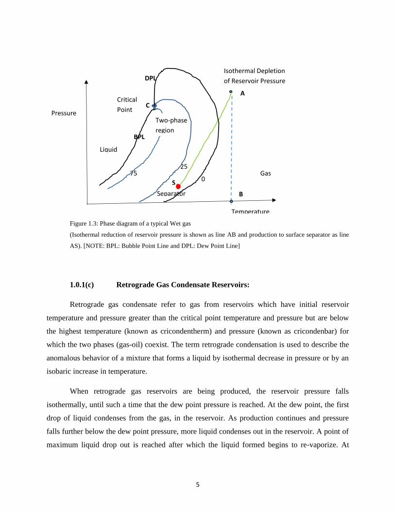
Figure 1.3: Phase diagram of a typical Wet gas
(Isothermal reduction of reservoir pressure is shown as line AB and production to surface separator as line
AS). [NOTE: BPL: Bubble Point Line and DPL: Dew Point Line]
1.0.1(c) Retrograde Gas Condensate Reservoirs:
Retrograde gas condensate refer to gas from reservoirs which have initial reservoir
temperature and pressure greater than the critical point temperature and pressure but are below
the highest temperature (known as cricondentherm) and pressure (known as cricondenbar) for
which the two phases (gas-oil) coexist. The term retrograde condensation is used to describe the
anomalous behavior of a mixture that forms a liquid by isothermal decrease in pressure or by an
isobaric increase in temperature.
When retrograde gas reservoirs are being produced, the reservoir pressure falls
isothermally, until such a time that the dew point pressure is reached. At the dew point, the first
drop of liquid condenses from the gas, in the reservoir. As production continues and pressure
falls further below the dew point pressure, more liquid condenses out in the reservoir. A point of
maximum liquid drop out is reached after which the liquid formed begins to re-vaporize. At
0
25 75 Gas
Separator
S
Pressure
Temperature
C
Liquid
A
Isothermal Depletion
of Reservoir Pressure
B
BPL
DPL
Critical
Point
Two-phase
region

6
abandonment pressure, all the liquid initially condensed in the reservoir do not re-vaporize and
get produced to the surface a situation, which can lead to loss of the condensed reservoir fluid.
This is not a welcome phenomenon because, not only is the trapped condensed oil lost in
the reservoir since it cannot be produced, the liquid droplets formed also creates blockages for
free flow of gas by reducing relative permeability to gas. The condensed oil is economically
more expensive and preferred to the gas and thus, it is best to produce most of it at the surface
where condensation would occur at the reduced separator temperature and pressure conditions.
One way of sustaining the reservoir pressure above the dew point pressure and thus
preventing the loss of condensates by its formation in the reservoir is by continuously circulating
light hydrocarbon inert gas into the reservoir. This has the ability of lightening the fluid and
improving recovery of high molecular weight hydrocarbons to the surface. At the surface, the
mixed fluid is passed through separators. The rich condensate is separated for sale and the light
gas may be recycled into the reservoir until such a time as most of the higher molecular weight
hydrocarbons which form condensates at the surface have been produced. This cyclic process is
referred to as gas cycling.
Generally speaking, gas condensates refer to any liquid condensed from a gas phase at
conditions of declining pressure at constant temperature, or simultaneous declining pressure and
temperature conditions. As such, three basic sources from which condensates can be produced
are recognized as: oil well gas plants, wet gas reservoirs and gas condensate reservoirs.
Normally, the greatest harvest of condensate is from retrograde gas condensate reservoirs
operated with cycling plants. A typical phase diagram for a gas condensate reservoir is shown
below as Figure 1.4.

7
Figure 1.4: Phase diagram of a typical Gas Condensate
(Isothermal reduction of reservoir pressure due to production is shown as line AB and production to surface
separator conditions is as shown by line AS. [NOTE: BPL: Bubble Point Line and DPL: Dew Point Line]
At temperatures and pressures in the vicinity of the critical points, marked 𝐶, in
Figure 1.2 through 1.4, the gas and liquid phases are exceedingly compressible and
possess large thermal expansions. Slight changes in pressure and/or temperature lead to
rapid changes in fluid properties. As the critical state is approached through the two
phase region there occurs a marked decrease in the viscosity of the liquid phase and a
corresponding increase in that of the gas phase, with a decrease in the interfacial tension.
The two phases become indistinguishable as the interfacial tension becomes zero and the
viscosities of the gas and liquid phases assume the same value.
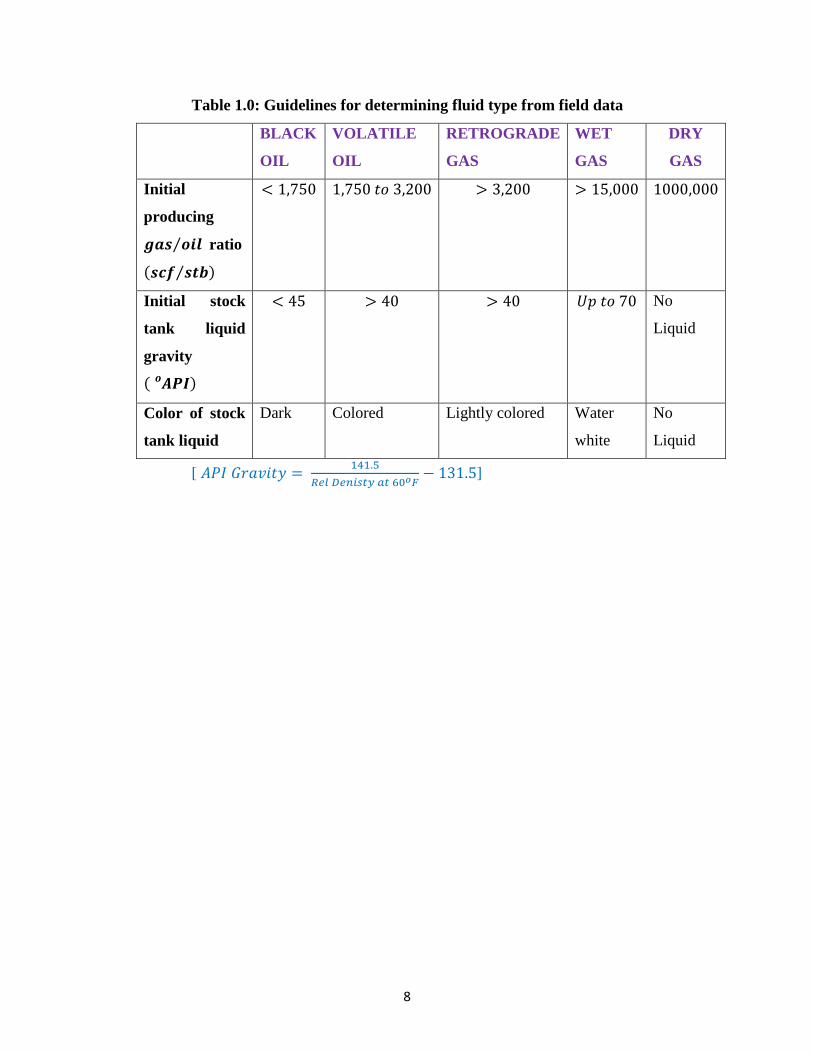
McCain (1994) provided a summary of guidelines for determining fluid type from
field data as shown below:
Pressure
Temperature
BPL
C
A
B
Two-Phase
Region
10
20 Gas
Cricondentherm
Critical
Point
Point
DPL
S
Reservoir pressure path
8
Table 1.0: Guidelines for determining fluid type from field data
BLACK
OIL
VOLATILE
OIL
RETROGRADE
GAS
WET
GAS
DRY
GAS
Initial
producing
𝒈𝒂𝒔 𝒐𝒊𝒍⁄ ratio
(𝒔𝒄𝒇 𝒔𝒕𝒃⁄ )
< 1,750 1,750 𝑡𝑜 3,200 > 3,200 > 15,000 1000,000
Initial stock
tank liquid
gravity
( 𝑨𝑷𝑰𝒐 )
< 45 > 40 > 40 𝑈𝑝 𝑡𝑜 70 No
Liquid
Color of stock
tank liquid
Dark Colored Lightly colored Water
white
No
Liquid
[ 𝐴𝑃𝐼 𝐺𝑟𝑎𝑣𝑖𝑡𝑦 = 141.5
𝑅𝑒𝑙 𝐷𝑒𝑛𝑖𝑠𝑡𝑦 𝑎𝑡 60𝑜𝐹− 131.5]
9
1.1 Obtaining Phase Behavior Data
Phase behavior data can be obtained from laboratory pressure-volume-
temperature (PVT) measurements or estimated from correlations such as equations of
state. Data from laboratory measurements are often more accurate but are associated with
such disadvantages as: susceptibility to human and precision errors, expensive in terms of
equipment and human hours invested, and concern for laboratory safety practices. Data
obtained theoretically by use of Equations of state (EOS) are tolerably accurate, faster
and less expensive to duplicate. The advent of high speed computers further simplifies
the application of equations of state to complex problems.
An equation of state (EOS) is defined simply as, a thermodynamic relationship
describing the state of matter under a given set of physical conditions, such as pressure,
volume and temperature (PVT). Cubic equations of state, (CEOSs) are expressed in terms
of molar volume or compressibility factor by polynomials of order three and are very
popular in the natural gas and chemical industry because they enjoy simplicity of form
and yet provide tolerable error limits. However, the prediction of liquid state densities
using the most popular Cubic equation of state results in considerable errors when
compared with experimentally determined values. Owing to this frustration, Valderrama
(2003) concluded that “the three parameters in cubic equations of state are inadequate in
capturing the intermolecular dynamics at the condensed state of liquids.”
This study has as its primary goal, to present a simple efficient three parameter
equation of state which would improve liquid density prediction in particular, and other
thermodynamic properties predictable by EOSs beyond that afforded by popular CEOS
such as Peng-Robinson’s and Patel-Teja’s EOSs without compromising on the simplicity
for which cubic EOSs are popular.
10
1.2Theoretical Background Information:
1.2.1 Equations of State (EOS):
Regardless of the aspect of petroleum extraction process, whether it be - drilling, reserve
estimation, reservoir performance analysis, reservoir simulation, tubing flow hydraulics,
gathering design, gas-liquid separation, oil and gas transmission, oil and gas metering or quality
control – a good predictive knowledge of phase behavior is required (Adewumi, 2014). The
behavior of fluids can be approximately represented by equations of state which are, simple
analytical expressions often relating pressure and volume to temperature or other thermodynamic
properties. These (EOSs) are constitutive equations which provide a mathematical relationship
between two or more state functions associated with the matter, such as its temperature, pressure,
volume, or internal energy.
1.2.1.1 USES OF EOSs: Equations of state are used:
1. for predicting the state of matter under a given set of physical conditions and for
describing transitions between states;
2. to predict phase equilibrium based on the equilibrium criterion:
𝑓𝑣 = 𝑓𝑙 = 𝑓𝑠;
3. for evaluation of gas injection processes (miscible and immiscible);
4. for evaluation off properties of a reservoir oil existing with a gas cap;
5. to estimate desired properties for extrapolating or interpolating PVT data when
attempting to model the behavior of reservoir fluids at various operating conditions of
temperature and pressure, particularly, for cases where there is no reservoir fluid data;
6. to correlate and predict thermodynamic and physical properties of fluids (pure
components and mixtures), supercritical phases and solids at a tiny fraction of the time
and cost required to obtain same information from laboratory measurements;
7. to correlate densities of gases and liquids to temperatures and pressures;
8. to simulate volatile and gas condensate production through constant volume depletion
evaluations;
11
9. to predict the phase behavior and volumetric properties of multi‐component systems,
these models can be used in reservoir, wellbore multi‐phase flow and pipeline modeling,
as well as design and operation of surface facilities;
10. For recombination tests using separator oil and gas streams;
11. In general, EOS models are employed to determine the properties and the amount of
equilibrated phases
1.2.2 Perfect Gases:
The simplest known equation of state is the perfect gas law, which is used for calculations of
thermodynamic properties for ideal gases, (also called perfect gases) or for real gases at normal
conditions such as standard temperature and pressure (temperatures, 𝑇 of about 60𝑜𝐹 =
520𝑜𝑅 = 288.72𝐾 and pressures, 𝑃 = 14.7 𝑝𝑠𝑖𝑎 = 101.325 𝐾𝑃𝑎), at which they
approximate ideal gas behavior. The Perfect gas is in fact, an idealization of real gases as no gas
is truly ideal. It is the simplest type of gas.
A perfect gas is by definition, one in which
(i) the volume occupied by the molecules is quite small and insignificant when compared
to the total gas volume, or the mean free path between two collisions.
(ii) the particles move in continuous straight lines and change of particle direction may
only result from localized collisions between particles. The collision events are
always two-body processes, and are perfectly elastic, that is, no energy is lost upon
collision, and
(iii) inter-molecular interactions (attractive or repulsive forces) do not exist.
The analytical expression of the PVT behavior of the hypothetical perfect gas behavior is
written as:
𝑃𝑉 = 𝑛𝑅𝑇 (1.0)
Where, 𝑛 is number of moles of gas, P is the pressure of the fluid; R is the universal gas constant,
and T is the absolute temperature. V is the molar volume of the container containing the fluid.
12
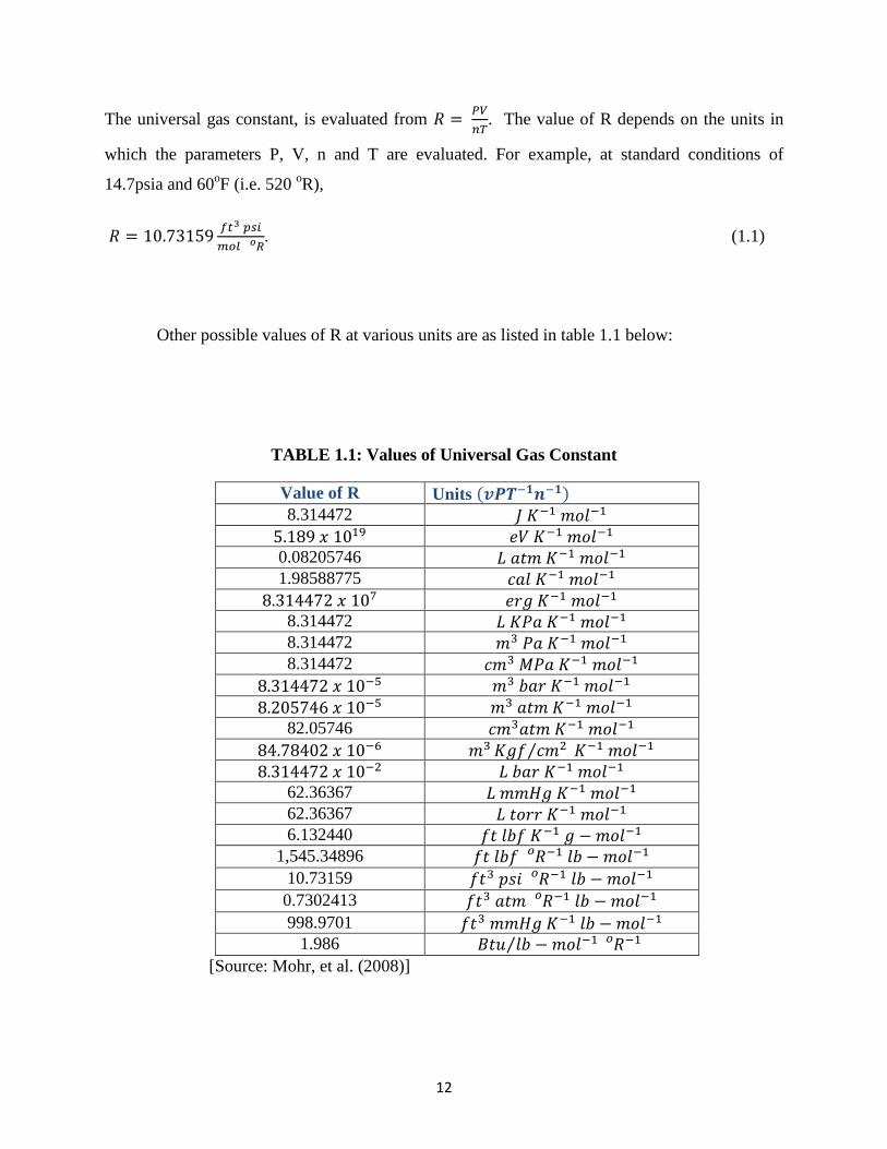
The universal gas constant, is evaluated from 𝑅 = 𝑃𝑉
𝑛𝑇. The value of R depends on the units in
which the parameters P, V, n and T are evaluated. For example, at standard conditions of
14.7psia and 60oF (i.e. 520
oR),
𝑅 = 10.73159𝑓𝑡3 𝑝𝑠𝑖
𝑚𝑜𝑙 𝑅𝑜 . (1.1)
Other possible values of R at various units are as listed in table 1.1 below:
TABLE 1.1: Values of Universal Gas Constant
Value of R Units (𝒗𝑷𝑻−𝟏𝒏−𝟏)
8.314472 𝐽 𝐾−1 𝑚𝑜𝑙−1
5.189 𝑥 1019 𝑒𝑉 𝐾−1 𝑚𝑜𝑙−1
0.08205746 𝐿 𝑎𝑡𝑚 𝐾−1 𝑚𝑜𝑙−1
1.98588775 𝑐𝑎𝑙 𝐾−1 𝑚𝑜𝑙−1
8.314472 𝑥 107 𝑒𝑟𝑔 𝐾−1 𝑚𝑜𝑙−1
8.314472 𝐿 𝐾𝑃𝑎 𝐾−1 𝑚𝑜𝑙−1
8.314472 𝑚3 𝑃𝑎 𝐾−1 𝑚𝑜𝑙−1
8.314472 𝑐𝑚3 𝑀𝑃𝑎 𝐾−1 𝑚𝑜𝑙−1
8.314472 𝑥 10−5 𝑚3 𝑏𝑎𝑟 𝐾−1 𝑚𝑜𝑙−1
8.205746 𝑥 10−5 𝑚3 𝑎𝑡𝑚 𝐾−1 𝑚𝑜𝑙−1
82.05746 𝑐𝑚3𝑎𝑡𝑚 𝐾−1 𝑚𝑜𝑙−1
84.78402 𝑥 10−6 𝑚3 𝐾𝑔𝑓 𝑐𝑚2⁄ 𝐾−1 𝑚𝑜𝑙−1
8.314472 𝑥 10−2 𝐿 𝑏𝑎𝑟 𝐾−1 𝑚𝑜𝑙−1
62.36367 𝐿 𝑚𝑚𝐻𝑔 𝐾−1 𝑚𝑜𝑙−1
62.36367 𝐿 𝑡𝑜𝑟𝑟 𝐾−1 𝑚𝑜𝑙−1
6.132440 𝑓𝑡 𝑙𝑏𝑓 𝐾−1 𝑔 − 𝑚𝑜𝑙−1
1,545.34896 𝑓𝑡 𝑙𝑏𝑓 𝑅𝑜 −1 𝑙𝑏 − 𝑚𝑜𝑙−1
10.73159 𝑓𝑡3 𝑝𝑠𝑖 𝑅𝑜 −1 𝑙𝑏 − 𝑚𝑜𝑙−1
0.7302413 𝑓𝑡3 𝑎𝑡𝑚 𝑅𝑜 −1 𝑙𝑏 − 𝑚𝑜𝑙−1
998.9701 𝑓𝑡3 𝑚𝑚𝐻𝑔 𝐾−1 𝑙𝑏 − 𝑚𝑜𝑙−1
1.986 𝐵𝑡𝑢 𝑙𝑏 − 𝑚𝑜𝑙−1⁄ 𝑅𝑜 −1 [Source: Mohr, et al. (2008)]
13
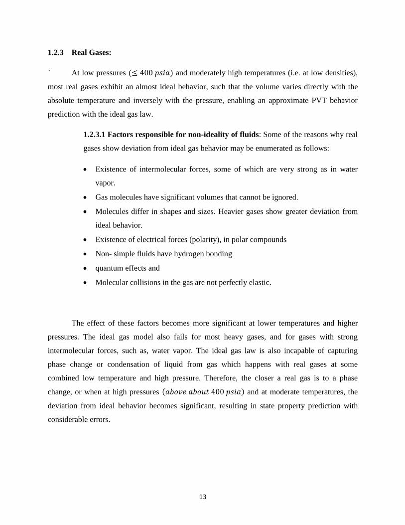
1.2.3 Real Gases:
` At low pressures (≤ 400 𝑝𝑠𝑖𝑎) and moderately high temperatures (i.e. at low densities),
most real gases exhibit an almost ideal behavior, such that the volume varies directly with the
absolute temperature and inversely with the pressure, enabling an approximate PVT behavior
prediction with the ideal gas law.
1.2.3.1 Factors responsible for non-ideality of fluids: Some of the reasons why real
gases show deviation from ideal gas behavior may be enumerated as follows:
Existence of intermolecular forces, some of which are very strong as in water
vapor.
Gas molecules have significant volumes that cannot be ignored.
Molecules differ in shapes and sizes. Heavier gases show greater deviation from
ideal behavior.
Existence of electrical forces (polarity), in polar compounds
Non- simple fluids have hydrogen bonding
quantum effects and
Molecular collisions in the gas are not perfectly elastic.
The effect of these factors becomes more significant at lower temperatures and higher
pressures. The ideal gas model also fails for most heavy gases, and for gases with strong
intermolecular forces, such as, water vapor. The ideal gas law is also incapable of capturing
phase change or condensation of liquid from gas which happens with real gases at some
combined low temperature and high pressure. Therefore, the closer a real gas is to a phase
change, or when at high pressures (𝑎𝑏𝑜𝑣𝑒 𝑎𝑏𝑜𝑢𝑡 400 𝑝𝑠𝑖𝑎) and at moderate temperatures, the
deviation from ideal behavior becomes significant, resulting in state property prediction with
considerable errors.

14
1.2.3.2 Compressibility Factor:
The deviation of a real gas from ideality can be quantified using the
compressibility factor denoted by ‘𝑧’. Gas compressibility factor, also known as gas
deviation factor or simply, z-factor is, by definition, the ratio of the molar volume of a
gas to the molar volume of an ideal gas at the same temperature and pressure.
By definition, z-factor is the ratio of the actual volume occupied by a mass of gas
at some pressure and temperature to the volume the gas would occupy if it behaved
ideally. This is written mathematically as:
𝑍 =𝑉𝑎𝑐𝑡𝑢𝑎𝑙
𝑉𝑖𝑑𝑒𝑎𝑙 or 𝑉𝑎𝑐𝑡𝑢𝑎𝑙 = 𝑍𝑉𝑖𝑑𝑒𝑎𝑙 (1.2)
The equation of state is 𝑃𝑉𝑖𝑑𝑒𝑎𝑙 = 𝑛𝑅𝑇
Or 𝑃𝑉𝑎𝑐𝑡𝑢𝑎𝑙
𝑍= 𝑛𝑅𝑇 (1.3)
Therefore, the equation of state for any gas is
𝑃𝑉 = 𝑍𝑛𝑅𝑇 (1.4)
And for one mole of gas, that is, for molar volume,
𝑃𝑉 = 𝑍𝑅𝑇 (1.5)
Where, for an ideal gas, 𝑧 = 1.0. A real gas with a 𝑧 𝑓𝑎𝑐𝑡𝑜𝑟 of 1.0 will behave in the
same way as an ideal gas would. Most gases compress more than an ideal gas at low
pressures, whereas the opposite is true at high pressures. The value of the correction
factor, 𝑍, generally increases with pressure and decreases with temperature. Therefore,
𝑧 𝑓𝑎𝑐𝑡𝑜𝑟 values can be positive or negative. At high pressures molecules are colliding
more often. This allows repulsive forces between molecules to have a noticeable
effect, making the molar volume of the real gas (𝑉𝑚)𝑟𝑒𝑎𝑙 𝑔𝑎𝑠 to be greater than the
molar volume of the corresponding ideal gas (𝑉𝑚)𝑖𝑑𝑒𝑎𝑙 𝑔𝑎𝑠, which causes 𝑍 to exceed
the value, 1.0 (Boublik, 1981). When pressures are lower, the molecules are free to
15
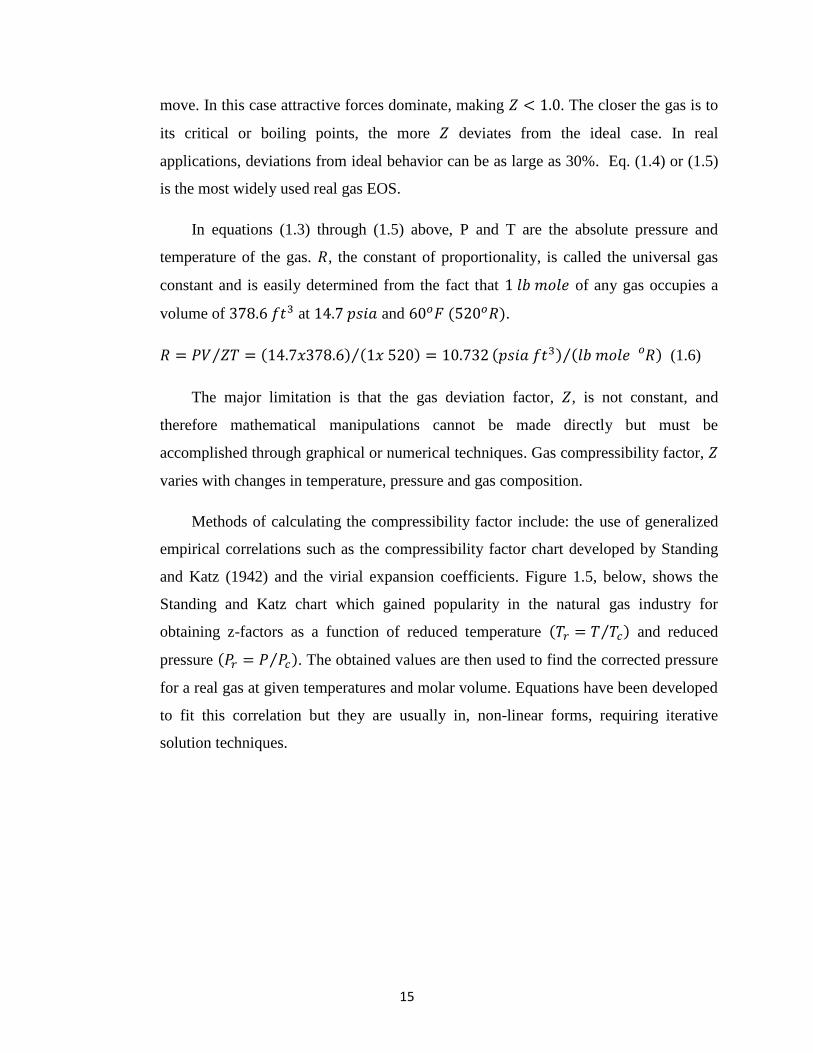
move. In this case attractive forces dominate, making 𝑍 < 1.0. The closer the gas is to
its critical or boiling points, the more 𝑍 deviates from the ideal case. In real
applications, deviations from ideal behavior can be as large as 30%. Eq. (1.4) or (1.5)
is the most widely used real gas EOS.
In equations (1.3) through (1.5) above, P and T are the absolute pressure and
temperature of the gas. 𝑅, the constant of proportionality, is called the universal gas
constant and is easily determined from the fact that 1 𝑙𝑏 𝑚𝑜𝑙𝑒 of any gas occupies a
volume of 378.6 𝑓𝑡3 at 14.7 𝑝𝑠𝑖𝑎 and 60𝑜𝐹 (520𝑜𝑅).
𝑅 = 𝑃𝑉 𝑍𝑇⁄ = (14.7𝑥378.6) (1𝑥 520) = 10.732 (𝑝𝑠𝑖𝑎 𝑓𝑡3) (𝑙𝑏 𝑚𝑜𝑙𝑒 𝑅𝑜 )⁄⁄ (1.6)
The major limitation is that the gas deviation factor, 𝑍, is not constant, and
therefore mathematical manipulations cannot be made directly but must be
accomplished through graphical or numerical techniques. Gas compressibility factor, 𝑍
varies with changes in temperature, pressure and gas composition.
Methods of calculating the compressibility factor include: the use of generalized
empirical correlations such as the compressibility factor chart developed by Standing
and Katz (1942) and the virial expansion coefficients. Figure 1.5, below, shows the
Standing and Katz chart which gained popularity in the natural gas industry for
obtaining z-factors as a function of reduced temperature (𝑇𝑟 = 𝑇 𝑇𝑐⁄ ) and reduced
pressure (𝑃𝑟 = 𝑃 𝑃𝑐⁄ ). The obtained values are then used to find the corrected pressure
for a real gas at given temperatures and molar volume. Equations have been developed
to fit this correlation but they are usually in, non-linear forms, requiring iterative
solution techniques.

16
Figure 1.5: Standing and Katz Simple Fluid Compressibility Chart
[Source: Standing and Katz, 1942)
17
Compressibility factor graphs are prone to considerable errors when dealing with
strongly polar gases for which the positive and negative charge do not coincide.
Estimated errors for such cases may be as high as 15 to 20 percent. Inaccurate z-factors
can lead to serious consequences such as gas metering errors, inaccurate reserve
estimates reporting and a faulty premise for serious management decision taking.
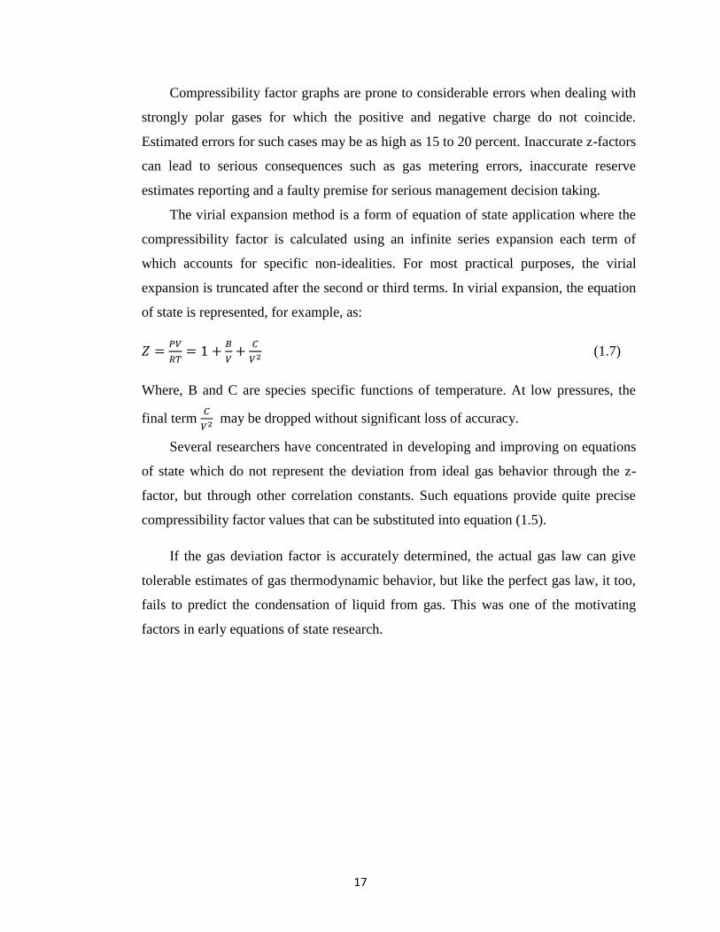
The virial expansion method is a form of equation of state application where the
compressibility factor is calculated using an infinite series expansion each term of
which accounts for specific non-idealities. For most practical purposes, the virial
expansion is truncated after the second or third terms. In virial expansion, the equation
of state is represented, for example, as:
𝑍 =𝑃𝑉
𝑅𝑇= 1 +
𝐵
𝑉+
𝐶
𝑉2 (1.7)
Where, B and C are species specific functions of temperature. At low pressures, the
final term 𝐶
𝑉2 may be dropped without significant loss of accuracy.
Several researchers have concentrated in developing and improving on equations
of state which do not represent the deviation from ideal gas behavior through the z-
factor, but through other correlation constants. Such equations provide quite precise
compressibility factor values that can be substituted into equation (1.5).
If the gas deviation factor is accurately determined, the actual gas law can give
tolerable estimates of gas thermodynamic behavior, but like the perfect gas law, it too,
fails to predict the condensation of liquid from gas. This was one of the motivating
factors in early equations of state research.

18
1.2.4 van der Waal’s Equation of State (vdW) (1873):
The earliest attempt to correct for the departure of real gases from ideal gas behavior and
extend the use of the ideal gas EOS to account for vapor-liquid co-existence was made by
Johannes Diderick van der Waals in 1873. In defending his PhD dissertation at the University of
Leiden, Netherlands, in 1873, van der Waals presented an improved solution to the capillary
problem and a new equation of state, based on general assumptions, Clausius’ virial theorem,
and the kinetic theory of gases. Van der Waals findings revolutionized the study of equations of
state and earned him a Nobel Prize in 1910. Van der Waals’ equation of state has the form:
(𝑃 +𝑎
𝑉2) (𝑉 − 𝑏) = 𝑅(1+∝ 𝑡) (1.8)
Where, 𝑃 is the external pressure, 𝑉 is the molar volume, ∝ is a constant related to the kinetic
energy of the molecule, 𝑎 is the “specific attraction” and 𝑏 is a multiple of the molecular volume.
Eq. (1.8) later became what is today known as the van der Waal’s equation of state (vdW):
𝑃 =𝑅𝑇
(𝑉−𝑏)−
𝑎
𝑉2 (1.9)
The constants 𝑎 and 𝑏 have positive values and are characteristic of the individual gases shown
in table below:
TABLE 1.2 : van der Waals’ Coefficients for Selected Substances
Gas Formula 𝑎(𝑎𝑡𝑚 𝐿2 𝑚𝑜𝑙−2) 𝑏(10−2 𝐿 𝑚𝑜𝑙−1)
Helium 𝐻𝑒 0.0341 2.380
Argon 𝐴𝑟 1.363 3.219
Nitrogen 𝑁2 1.408 3.913
Carbon dioxide 𝐶𝑂2 3.640 4.267
Methanol 𝐶𝐻3𝑂𝐻 9.23 6.510
Hydrogen 𝐻2 0.244 2.66
Ethane 𝐶2𝐻6 5.49 6.38
Water 𝐻2𝑂 5.46 3.05
Ammonia 𝑁𝐻3 4.17 3.71

19
The vdW coefficients are found by fitting the calculated curves to the experimental
curves. They are characteristic of each gas but independent of temperature.The equation of state
of van der Waals gives a qualitative description of the vapor and liquid phases and phase
transitions but it is rarely sufficiently accurate for critical properties and phase equilibria
calculations. A simple example is that for all fluids, the critical compressibility factor predicted
by Eq. (1.9) is 𝑍𝑐 =𝑃𝑐𝑉𝑐
𝑅𝑇𝑐=
3
8= 0.375. This does not agree with the experimental observations or
results which show that each chemical species has its own value of 𝑍𝑐with values that vary from
0.24 to 0.29.
After van der Waals’ pioneering work, equations of state have and continue to enjoy a
large amount of research interests. Several authors have sought to improve accuracy and have
indeed achieved a level of improvement by modifying either the repulsive term or the attractive
term of the original vdW’s EOS.
1.2.4.1 Modifications of vdW’s Repulsive Term:
The first significant modification of the vdW’s repulsive term was developed by Thiele
(1963). His modification has the form:
𝑃ℎ𝑠 =𝑅𝑇
(𝑉𝑚−𝑏)=
𝑅𝑇
𝑉𝑚(
1
1−𝑏
𝑉𝑚
) =𝑅𝑇
𝑉𝑚(
1−𝜂3
(1−𝜂)4) (1.10)
Where, 𝑃ℎ𝑠 represents a hard sphere equation of state and
𝜂 =𝑏
4𝑉𝑚 . (1.11)
Carnahan and Starling (1969) improved Thiele’s (1963) expression Eq. (1.10) to a form
(Eq. (1.12)) which became very popular and tends to give very good approximations for the
repulsive term.
𝑃ℎ𝑠 =𝑅𝑇
𝑉𝑚(
1+𝜂+𝜂2−𝜂3
[1−𝜂]3 ) (1.12)
20
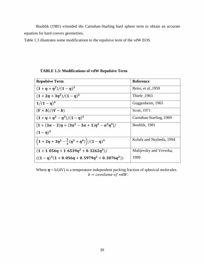
Boublik (1981) extended the Carnahan-Starling hard sphere term to obtain an accurate
equation for hard convex geometries.
Table 1.3 illustrates some modifications to the repulsive term of the vdW EOS.
TABLE 1.3: Modifications of vdW Repulsive Term
Repulsive Term Reference
(𝟏 + 𝜼 + 𝜼𝟐)/(𝟏 − 𝜼)𝟑 Reiss, et al.,1959
(𝟏 + 𝟐𝜼 + 𝟑𝜼𝟐)/(𝟏 − 𝜼)𝟐 Thiele ,1963
𝟏 (𝟏 − 𝜼)𝟒⁄ Guggenheim, 1965
(𝑽 + 𝒃) (𝑽 − 𝒃)⁄ Scott, 1971
(𝟏 + 𝜼 + 𝜼𝟐 − 𝜼𝟑)/(𝟏 − 𝜼)𝟑 Carnahan-Starling, 1969
[𝟏 + (𝟑𝜶 − 𝟐)𝜼 + (𝟑𝜶𝟐 − 𝟑𝜶 + 𝟏)𝜼𝟐 − 𝜶𝟐𝜼𝟑]/
(𝟏 − 𝜼)𝟑
Boublik, 1981
(𝟏 + 𝟐𝜼 + 𝟑𝜼𝟐 −𝟐
𝟑(𝜼𝟑 + 𝜼𝟒)) /(𝟏 − 𝜼)𝟑 Kolafa and Nezbeda, 1994
(𝟏 + 𝟏. 𝟎𝟓𝟔𝜼 + 𝟏. 𝟔𝟓𝟑𝟗𝜼𝟐 + 𝟎. 𝟑𝟐𝟔𝟐𝜼𝟑)/
((𝟏 − 𝜼)𝟑(𝟏 + 𝟎. 𝟎𝟓𝟔𝜼 + 𝟎. 𝟓𝟗𝟕𝟗𝜼𝟐 + 𝟎. 𝟑𝟎𝟕𝟔𝜼𝟑))
Malijevsky and Veverka,
1999
Where 𝜼 = b/(4V) is a temperature independent packing fraction of spherical molecules.
𝑏 = 𝑐𝑜𝑣𝑜𝑙𝑢𝑚𝑒 𝑜𝑓 𝑣𝑑𝑊.

21
1.2.4.2 Modifications of vdW’s Attraction Term:
Since the 1980s there has been a trend to introduce temperature-dependent functions into
cubic equations, and most of the functions were determined from trial-and-error experiences, not
from strict or sound theories (Yun et al., 1998). More research is however concentrated on the
attractive term modification in recent years. Table 1.4 illustrates modifications to the attractive
term of the original vdW’s EOS.
TABLE 1.4: Modifications on vdW Attraction Term
Attractive Term Equation , Date
𝑎 𝑇0.5𝑉(𝑉 + 𝑏)⁄ Redlich-Kwong, 1949
𝑎(𝑇) 𝑉(𝑉 + 𝑏)⁄ Soave-Redlich-Kwong, 1972
𝑎(𝑇) 𝑉(𝑉 + 𝑏) + 𝑏(𝑉 − 𝑏)⁄ Peng-Robinson, 1976
𝑎(𝑇) 𝑉(𝑉 + 𝑐𝑏)⁄ Fuller, 1976
𝑎(𝑇) [𝑉2 + 𝑢𝑏𝑉 + 𝑤𝑏2]⁄ Schmidt-Wenzel, 1980
𝑎(𝑇) [𝑉2 + 𝑐𝑏𝑉 − (𝑐 − 1)𝑏2]⁄ Harmens-Knapp, 1980
𝑎(𝑇) [𝑉(𝑉 + 𝑏) + 𝑐(𝑉 − 𝑏)]⁄ Patel –Teja,1982
𝑎(𝑇) (𝑉 + 𝑐)2⁄ Kubic, 1982
𝑎(𝑇) [(𝑉 − 𝑏2)(𝑉 + 𝑏3)]⁄ Adachi, et al., 1983
𝑎(𝑇) [𝑉2 + 2𝑏𝑉 − 𝑏2]⁄ Stryjek-Vera, 1986
𝑎(𝑇) [𝑉(𝑉 + 𝑐) + 𝑏(3𝑉 + 𝑐)]⁄ Yu and Lu, 1987
𝑎(𝑇) [(𝑉 + 𝑐)(𝑉 + 2𝑐 + 𝑏]⁄ Trebble and Bishnoi, 1987
22
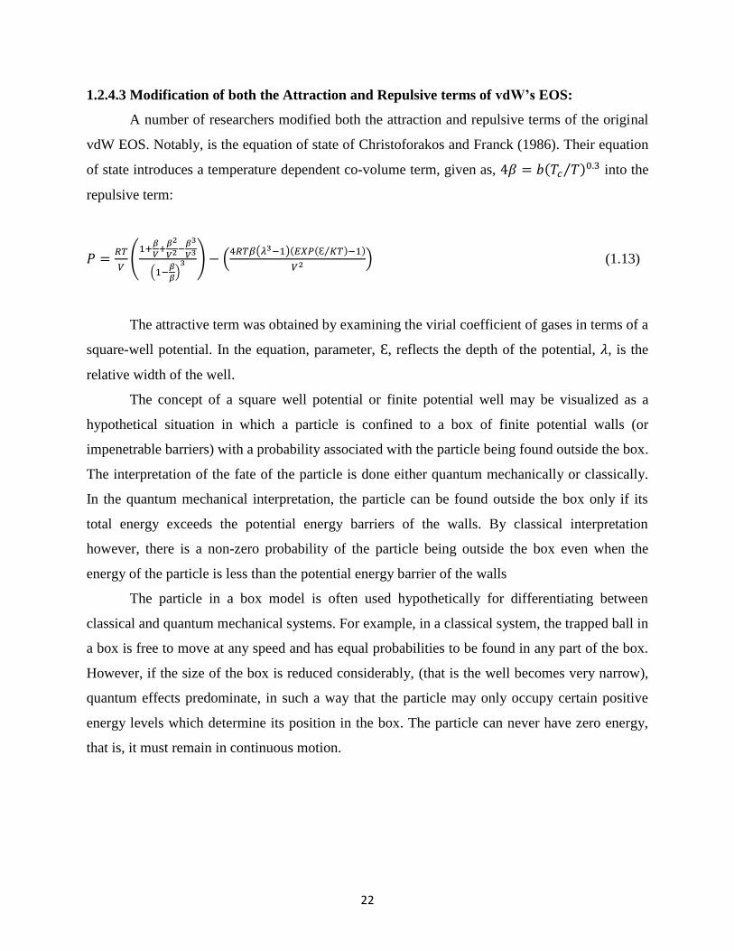
1.2.4.3 Modification of both the Attraction and Repulsive terms of vdW’s EOS:
A number of researchers modified both the attraction and repulsive terms of the original
vdW EOS. Notably, is the equation of state of Christoforakos and Franck (1986). Their equation
of state introduces a temperature dependent co-volume term, given as, 4𝛽 = 𝑏(𝑇𝑐 𝑇⁄ )0.3 into the
repulsive term:
𝑃 =𝑅𝑇
𝑉(
1+𝛽
𝑉+
𝛽2
𝑉2−𝛽3
𝑉3
(1−𝛽
𝛽)
3 ) − (4𝑅𝑇𝛽(𝜆3−1)(𝐸𝑋𝑃(Ԑ 𝐾𝑇⁄ )−1)
𝑉2 ) (1.13)
The attractive term was obtained by examining the virial coefficient of gases in terms of a
square-well potential. In the equation, parameter, Ԑ, reflects the depth of the potential, 𝜆, is the
relative width of the well.
The concept of a square well potential or finite potential well may be visualized as a
hypothetical situation in which a particle is confined to a box of finite potential walls (or
impenetrable barriers) with a probability associated with the particle being found outside the box.
The interpretation of the fate of the particle is done either quantum mechanically or classically.
In the quantum mechanical interpretation, the particle can be found outside the box only if its
total energy exceeds the potential energy barriers of the walls. By classical interpretation
however, there is a non-zero probability of the particle being outside the box even when the
energy of the particle is less than the potential energy barrier of the walls
The particle in a box model is often used hypothetically for differentiating between
classical and quantum mechanical systems. For example, in a classical system, the trapped ball in
a box is free to move at any speed and has equal probabilities to be found in any part of the box.
However, if the size of the box is reduced considerably, (that is the well becomes very narrow),
quantum effects predominate, in such a way that the particle may only occupy certain positive
energy levels which determine its position in the box. The particle can never have zero energy,
that is, it must remain in continuous motion.
23
1.3 Classification and Interrelationship between Different EOSs:
Since the work of van der Waals (1873), interest in the field of equation of state
development and/or modification has remained active, giving rise to many equations differing in
form and complexities. The complex EOS’s give good predictions of both phase equilibriums
and volumetric properties but require large number of experimental data. Firoozabadi (1989)
noted that, non-cubic equations of state, as they are sometimes called, when compared to the
popular cubic EOSs, give better descriptions of the volumetric behavior of pure substances but
may not be suitable for complex hydrocarbon mixtures The application of multi parameter EOSs
such as the Bennedict-Webb-Rubin’s (BWR) type equations demands a high computational time
and effort, due to their high powers in volume and large number of parameters, hence, unsuitable
for reservoir fluid studies where many sequential equilibrium calculations are required.
The cubic equations of state have become more popular over the years because of their
structural simplicity and acceptable accuracy. In general, they require only a few parameters for
implementation and little computer resources and give good phase equilibrium correlations and
saturated phase volumes and densities. This guarantees a comparatively lower computational
overhead of the cubic EOS’s when compared to the other two categories.
The relentless effort of researchers to improve accuracy has extended the traditional two
parameters associated with the van der Waals cubic EOS to three and even four parameter type
EOS’s. Therefore, cubic EOS’s can now be broadly classified according to the number of
independent parameters characterizing the molecular properties of the individual components.
A substantial inter-relationship between various different equations of state exist since
new equations of state are proposed as modifications of existing ones, or successful components
of one or more equations of state are reused to form a new equation. This component reuse is
common to both empirical and theoretical equations of state. Invariably, equations of state are
formed by combining separate contributions from repulsive and attractive terms interactions. It is
very rare for an equation of state to be developed entirely from scratch. EOS classification can be
varied depending on basis of interest.
Based on formulation and functionality, equations of state can be broadly categorized
into three: non-analytic (or empirical), virial and semi-theoretical (or semi-empirical).

24
1.3.1 Non-Analytic (or Empirical) Equations of State
This group of equations of state usually contains high order polynomials or large number
of substance-specific parameters (multi-parameters) that require fitting to large amount of
experimental data of several properties. These parameters have physical meanings. Such
equations (also called reference equations) are typically designed for one or at most a few
compounds.
Empirical Equations of States can be categorized into two major classes. One uses a two-
point tensor that transforms as a second rank tensor under transformation of spatial coordinates
and transforms as a scalar under transformation of the material coordinates (also called Eulerian
strain) or Interatomic potential EOSs and refines their parameters in order to find a better fit to
experiments. The interatomic potential describes the interaction between a pair of atoms or the
interaction of an atom with a group of atoms in a condensed phase. The potential must have both
an attractive and a repulsive component if binding is to occur.
The other approach seeks to find mathematical function or relationships which give the
best fit to the experiments. The accuracy of empirical equations of state is often limited to their
target fluids and within the range of thermodynamic conditions for which their parameters were
fitted. The resulting equation cannot often be used to extrapolate with confidence outside the
interpolation region. They are however, applicable over much broader ranges of P and T than are
the analytic equations. Most empirical equations of state may fail to represent the properties of
pure fluids within the critical region since reliable experimental data closer to the critical point
are often lacking.
1.3.2 The Virial-Type Equations of State
This group of equations characteristically, requires a large number of experimental data
for parameterization and often consists of multi-parameters. They are generally, good volume
predictors but give poor representations of phase equilibriums. This group of equations of state,
also called theoretical equations of state and based on the theory of statistical mechanics, was
first proposed for real gases in 1901 by Heike kamerlingh-Onnes, a Dutch physicist and Nobel
Laureate. Karmerlingh-Onnes, winner of the Nobel Prize in physics in 1913 had in 1901,
developed the original equation of van der Waals in series using the following arguments.
25
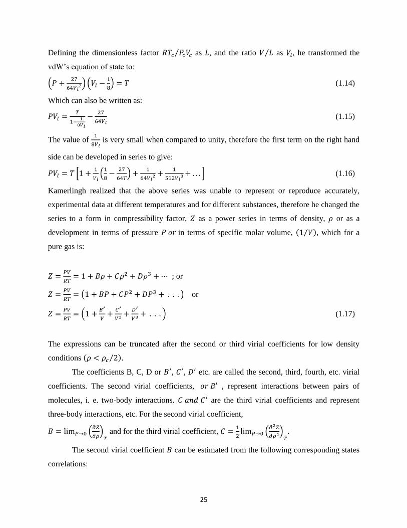
Defining the dimensionless factor 𝑅𝑇𝑐 𝑃𝑐𝑉𝑐⁄ as 𝐿, and the ratio 𝑉 𝐿⁄ as 𝑉𝑙, he transformed the
vdW’s equation of state to:
(𝑃 +27
64𝑉𝑙2) (𝑉𝑙 −
1
8) = 𝑇 (1.14)
Which can also be written as:
𝑃𝑉𝑙 =𝑇
1−1
8𝑉𝑙
−27
64𝑉𝑙 (1.15)
The value of 1
8𝑉𝑙 is very small when compared to unity, therefore the first term on the right hand
side can be developed in series to give:
𝑃𝑉𝑙 = 𝑇 [1 +1
𝑉𝑙(
1
8−
27
64𝑇) +
1
64𝑉𝑙2 +
1
512𝑉𝑙3 + . . . ] (1.16)
Kamerlingh realized that the above series was unable to represent or reproduce accurately,
experimental data at different temperatures and for different substances, therefore he changed the
series to a form in compressibility factor, 𝑍 as a power series in terms of density, 𝜌 or as a
development in terms of pressure 𝑃 𝑜𝑟 in terms of specific molar volume, (1 𝑉⁄ ), which for a
pure gas is:
𝑍 =𝑃𝑉
𝑅𝑇= 1 + 𝐵𝜌 + 𝐶𝜌2 + 𝐷𝜌3 + ⋯ ; or
𝑍 =𝑃𝑉
𝑅𝑇= (1 + 𝐵𝑃 + 𝐶𝑃2 + 𝐷𝑃3 + . . . ) or
𝑍 =𝑃𝑉
𝑅𝑇= (1 +
𝐵′
𝑉+
𝐶′
𝑉2 +𝐷′
𝑉3 + . . . ) (1.17)
The expressions can be truncated after the second or third virial coefficients for low density
conditions (𝜌 < 𝜌𝑐 2⁄ ).
The coefficients B, C, D or 𝐵′, 𝐶′, 𝐷′ etc. are called the second, third, fourth, etc. virial
coefficients. The second virial coefficients, 𝑜𝑟 𝐵′ , represent interactions between pairs of
molecules, i. e. two-body interactions. 𝐶 𝑎𝑛𝑑 𝐶′ are the third virial coefficients and represent
three-body interactions, etc. For the second virial coefficient,
𝐵 = lim𝑃→0 (𝜕𝑍
𝜕𝜌)
𝑇 and for the third virial coefficient, 𝐶 =
1
2lim𝑃→0 (
𝜕2𝑍
𝜕𝜌2)𝑇.
The second virial coefficient 𝐵 can be estimated from the following corresponding states
correlations:

26
𝐵0 = 0.083 −0.422
𝑇𝑟1.6 (1.18)
𝐵1 = 0.139 −0.172
𝑇𝑟4.2 (1.19)
𝐵 =𝑅𝑇𝑐
𝑃𝑐(𝐵0 + 𝜔𝐵1) (1.20)
Where, 𝜔 is the acentric factor.
Virial coefficients are substance and temperature dependent. This means they will be
functions of temperature and have specific parameters for different fluid molecules as seen in the
table below:
TABLE 1.5: Second and Third Virial Coefficients at 𝟐𝟗𝟖. 𝟏𝟓𝑲
𝑮𝑨𝑺 𝑩(𝟏𝟎−𝟔𝒎𝟑𝒎𝒐𝒍−𝟏) 𝑪(𝟏𝟎−𝟏𝟐𝒎𝟔𝒎𝒐𝒍−𝟐)
𝐻2 14.1 350
𝐻𝑒 11.8 121
𝑁2 −4.5 1100
𝑂2 −16.1 1200
𝐴𝑟 −15.8 1160
𝐶𝑂 −8.6 1550
At low temperatures, the second virial coefficient is negative since the long range
attractive molecular forces are dominant. This tends to reduce the pressure of the fluid below that
of an ideal gas. As the temperature increases, the second virial coefficient becomes less negative
as molecular interactions become more energetic, increasing the contribution of short range
repulsive forces and thereby increasing pressure. The higher order virial coefficients are very
difficult to determine empirically due to lack of sufficient experimental data. They may,
however, be theoretically derived from molecular theory, but such computations are also, very
difficult. For these reasons, the equation is generally truncated at the second coefficient, which
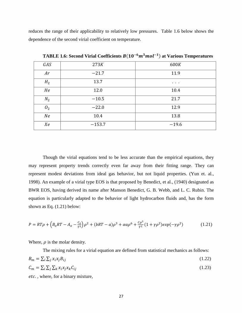
27
reduces the range of their applicability to relatively low pressures. Table 1.6 below shows the
dependence of the second virial coefficient on temperature.
TABLE 1.6: Second Virial Coefficients 𝑩(𝟏𝟎−𝟔𝒎𝟑𝒎𝒐𝒍−𝟏) at Various Temperatures
𝐺𝐴𝑆 273𝐾 600𝐾
𝐴𝑟 −21.7 11.9
𝐻2 13.7 . . .
𝐻𝑒 12.0 10.4
𝑁2 −10.5 21.7
𝑂2 −22.0 12.9
𝑁𝑒 10.4 13.8
𝑋𝑒 −153.7 −19.6
Though the virial equations tend to be less accurate than the empirical equations, they
may represent property trends correctly even far away from their fitting range. They can
represent modest deviations from ideal gas behavior, but not liquid properties. (Yun et. al.,
1998). An example of a virial type EOS is that proposed by Benedict, et al., (1940) designated as
BWR EOS, having derived its name after Manson Benedict, G. B. Webb, and L. C. Rubin. The
equation is particularly adapted to the behavior of light hydrocarbon fluids and, has the form
shown as Eq. (1.21) below:
𝑃 = 𝑅𝑇𝜌 + (𝐵𝑜𝑅𝑇 − 𝐴𝑜 −𝐶𝑜
𝑇2) 𝜌2 + (𝑏𝑅𝑇 − 𝑎)𝜌3 + 𝛼𝑎𝜌6 +𝐶𝜌3
𝑇2(1 + 𝛾𝜌2)𝑒𝑥𝑝(−𝛾𝜌2) (1.21)
Where, 𝜌 is the molar density.
The mixing rules for a virial equation are defined from statistical mechanics as follows:
𝐵𝑚 = ∑ ∑ 𝑥𝑖𝑥𝑗𝐵𝑖𝑗𝑗𝑖 (1.22)
𝐶𝑚 = ∑ ∑ ∑ 𝑥𝑖𝑥𝑗𝑥𝑘𝐶𝑖𝑗𝑘𝑗𝑖 (1.23)
𝑒𝑡𝑐. , where, for a binary mixture,

28
𝐵𝑚 = 𝑥12𝐵11 + 𝑥1𝑥2(𝐵12 + 𝐵21) + 𝑥2
2𝐵221 (1.24)
𝐶𝑚 = 𝑥13𝐶111 + 𝑥1
2𝑥2(𝐶112 + 𝐶121 + +𝐶211) + 𝑥1𝑥22(𝐶122 + 𝐶212 + +𝐶221) + 𝑥2
3𝐶222
(1.25)
1.3.3 Semi-Theoretical (or Semi-Empirical) EOSs
This group of equations of state combines features of theoretical and empirical equations.
That is, molecular parameters in a theoretically derived equation of state are fitted to
experimental data. They are often cubic or quadric in volume, which guarantees that the volumes
can be calculated analytically from specified temperatures and pressures. This group of equations
can represent both liquid and vapor behavior over limited ranges of temperature and pressure for
many but not all substances. Their predictive abilities often depend on the quality of the
theoretical basis used.
The molecular based EOSs consisting of such sub-groups as the perturbation models,
chemical theory equations for strongly associating species, and crossover relations are generally
semi-empirically derived. This group of EOSs assumes that there are three major contributions to
the total intermolecular potential of a given molecule: the repulsion-dispersion contribution
typical of individual segments, the contribution due to the fact that these segments can form a
chain, and the contribution due to the possibility that some segment- (s) form association
complexes with other molecules. Within the framework of the Statistical Associating Fluid
theory, (SAFT), the residual Helmholtz energy, defined as the difference between the total molar
Helmholtz energy and that of an ideal gas at the same temperature T and molar density 𝜌 is given
by:
𝑎𝑟(𝑇, 𝜌) = 𝑎(𝑇, 𝜌) − 𝑎𝑖𝑑𝑒𝑎𝑙 𝑔𝑎𝑠(𝑇, 𝜌) (1.26)
and 𝑎𝑟 = 𝑎𝑠𝑒𝑔 + 𝑎𝑐ℎ𝑎𝑖𝑛 + 𝑎𝑎𝑠𝑠𝑜𝑐 (1.27)
Where, the superscripts ‘seg’, ‘chain’, and ‘assoc’ refer to the contributions from the
“monomeric” segments, from the formation of chains, and from the existence of association
sites, respectively.
29
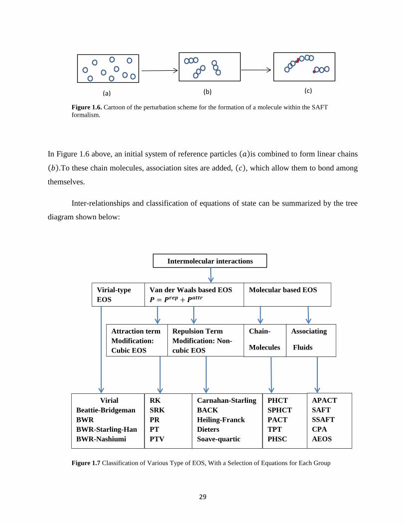
Figure 1.6. Cartoon of the perturbation scheme for the formation of a molecule within the SAFT
formalism.
In Figure 1.6 above, an initial system of reference particles (𝑎)is combined to form linear chains
(𝑏).To these chain molecules, association sites are added, (𝑐), which allow them to bond among
themselves.
Inter-relationships and classification of equations of state can be summarized by the tree
diagram shown below:
Figure 1.7 Classification of Various Type of EOS, With a Selection of Equations for Each Group
Intermolecular interactions
Virial-type
EOS
Van der Waals based EOS
𝑷 = 𝑷𝒓𝒆𝒑 + 𝑷𝒂𝒕𝒕𝒓
Molecular based EOS
Virial
Beattie-Bridgeman
BWR
BWR-Starling-Han
BWR-Nashiumi
Attraction term
Modification:
Cubic EOS
Repulsion Term
Modification: Non-
cubic EOS
Chain-
Molecules
Associating
Fluids
RK
SRK
PR
PT
PTV
Carnahan-Starling
BACK
Heiling-Franck
Dieters
Soave-quartic
PHCT
SPHCT
PACT
TPT
PHSC
APACT
SAFT
SSAFT
CPA
AEOS
(a) (b) (c)
30
1.4 Solution Methods for Cubic Equations of State
Different methods exist for the solution of cubic equations of state. The methods are
classified boldly into analytical, semi-analytic, numerical, graphical and use of software
schemes. Some of the very popular methods are summarized below. It is important to note and
remind here, that for any cubic expression of the form:
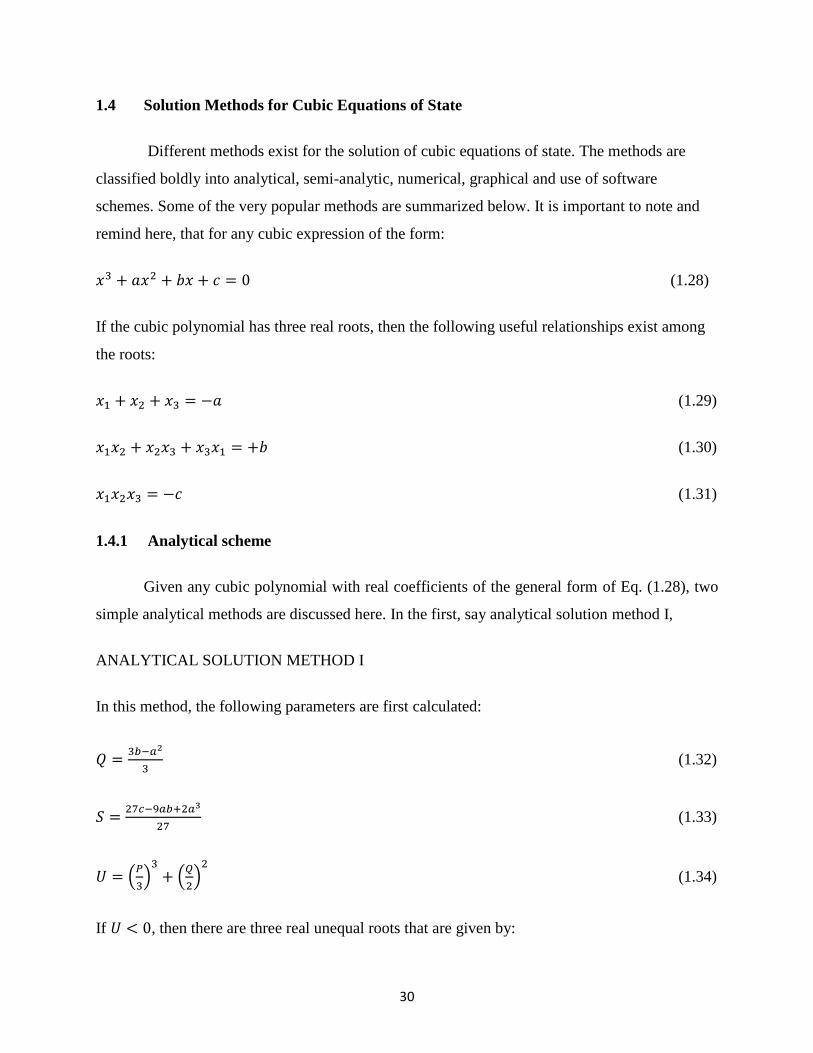
𝑥3 + 𝑎𝑥2 + 𝑏𝑥 + 𝑐 = 0 (1.28)
If the cubic polynomial has three real roots, then the following useful relationships exist among
the roots:
𝑥1 + 𝑥2 + 𝑥3 = −𝑎 (1.29)
𝑥1𝑥2 + 𝑥2𝑥3 + 𝑥3𝑥1 = +𝑏 (1.30)
𝑥1𝑥2𝑥3 = −𝑐 (1.31)
1.4.1 Analytical scheme
Given any cubic polynomial with real coefficients of the general form of Eq. (1.28), two
simple analytical methods are discussed here. In the first, say analytical solution method I,
ANALYTICAL SOLUTION METHOD I
In this method, the following parameters are first calculated:
𝑄 =3𝑏−𝑎2
3 (1.32)
𝑆 =27𝑐−9𝑎𝑏+2𝑎3
27 (1.33)
𝑈 = (𝑃
3)
3
+ (𝑄
2)
2
(1.34)
If 𝑈 < 0, then there are three real unequal roots that are given by:

31
𝑥𝑛 = (−2 ∗ 𝑠𝑖𝑔𝑛(𝑆)√−𝑄
3) 𝑐𝑜𝑠 (
∅
3+ 120 ∗ 𝑛) −
𝑎
3 (1.35)
𝑛 = 1,2,3 (1.36)
∅ = 𝑐𝑜𝑠−1 (√(𝑆 2⁄ )2
−(𝑄 3⁄ )3), (1.37)
𝑠𝑖𝑔𝑛(𝑆) = (+1), 𝑖𝑓 𝑆 > 0(−1), 𝑖𝑓 𝑆 < 0
(1.38)
Where, the angle ∅ is in degrees.
ANALYTICAL SOLUTION METHOD II
Another easily applicable analytical solution method is one for which the first step is to calculate
the parameters:
𝑄 ≡𝑎2−3𝑏
9 (1.39)
and
𝑁 ≡2𝑎3−9𝑎𝑏+27𝑐
54 (1.40)
The value
M = N2 – Q
3 (1.41)
is let to be the discriminant. The following possible cases are then considered:
a. If M < 0 (i. e., N2 < Q
3), the polynomial has three real roots. For this case, compute
𝜃 = 𝑎𝑟𝑐𝑐𝑜𝑠 (𝑁
√𝑄3) (1.42)

32
in radians and the three distinct real roots are calculated using:
𝑥1 = − (2√𝑄𝑐𝑜𝑠𝜃
3) −
𝑎
3 (1.43)
𝑥2 = − (2√𝑄𝑐𝑜𝑠𝜃+2𝜋
3) −
𝑎
3 (1.44)
𝑥3 = − (2√𝑄𝑐𝑜𝑠𝜃−2𝜋
3) −
𝑎
3 (1.45)
where, 𝑥1, 𝑥2, 𝑥3 are not given in any special order.
b. If M > 0 (i. e., N2 > Q
3), the polynomial has only one real root. Compute:
𝑆 = √−𝑁 + √𝑀3
(1.46)
𝑈 = √−𝑁 − √𝑀3
(1.47)
and calculate the real root as follows:
𝑥1 = 𝑆 + 𝑈 −𝑎
3 (1.48)
Sometimes, the equations for S and U listed above cause problems while programming.
This usually happens whenever the computer/calculator performs the cubic root of a negative
quantity. If you want to avoid such a situation, you may compute S’ and U’ instead:
𝑆′ = −𝑠𝑖𝑔𝑛(𝑁)√𝑎𝑏𝑠(𝑁) + √𝑀3
(1.49)
𝑈′ =𝑄
𝑆′ (making 𝑈′ = 0 𝑤ℎ𝑒𝑛 𝑆′ = 0) (1.50)
Where, 𝑎𝑏𝑠(𝑁) = Absolute value of 𝑁 and
𝑠𝑖𝑔𝑛(𝑁) = (+1), 𝑖𝑓 𝑁 𝑖𝑠 𝑝𝑜𝑠𝑖𝑡𝑖𝑣𝑒(−1), 𝑖𝑓 𝑁 𝑖𝑠 𝑛𝑒𝑔𝑎𝑡𝑖𝑣𝑒
(1.51)
𝑠𝑖𝑔𝑛(𝑁) may be defined as:

33
𝑠𝑖𝑔𝑛(𝑁) =𝑁
𝐴𝐵𝑆(𝑁) (1.52)
and then the real root is:
𝑥1 = 𝑆′ + 𝑈′ −𝑎
3 (1.53)
1.4.2 Numerical Scheme
NUMERICAL METHOD I
In this method which is iterative, the equation may be expressed in terms of volume, so that the
generalized form of cubic equations takes the form:
𝐴𝑉3 + 𝐵𝑉2 + 𝐶𝑉 + 𝐷 = 0 (1.54)
An initial guess is made for the volume. An educated guess would be the ideal gas volume at the
temperature and pressure of interest. Using this as 𝑉𝑜𝑙𝑑, then evaluate:
𝑉𝑛𝑒𝑤 = −(1 𝐶⁄ )(𝐴𝑉𝑜𝑙𝑑3 + 𝐵𝑉𝑜𝑙𝑑
2 + 𝐷) (1.55)
Check if [𝑉𝑛𝑒𝑤 − 𝑉𝑜𝑙𝑑] is within some tolerance, such as 0.001. If so, 𝑉𝑛𝑒𝑤 is the required
volume, else, it is used as assigned to 𝑉𝑜𝑙𝑑, and used for the next iteration to calculate another
𝑉𝑛𝑒𝑤 value. That is,
𝑉𝑖+1 = −(1 𝐶⁄ )(𝐴𝑉𝑖3 + 𝐵𝑉𝑖
2 + 𝐷) (1.56)
Iteration continues in this mode until convergence is achieved, such that
(𝑉𝑖+1
𝑉𝑖) ≅ 0.99 𝑡𝑜 1.01. (1.57)
34
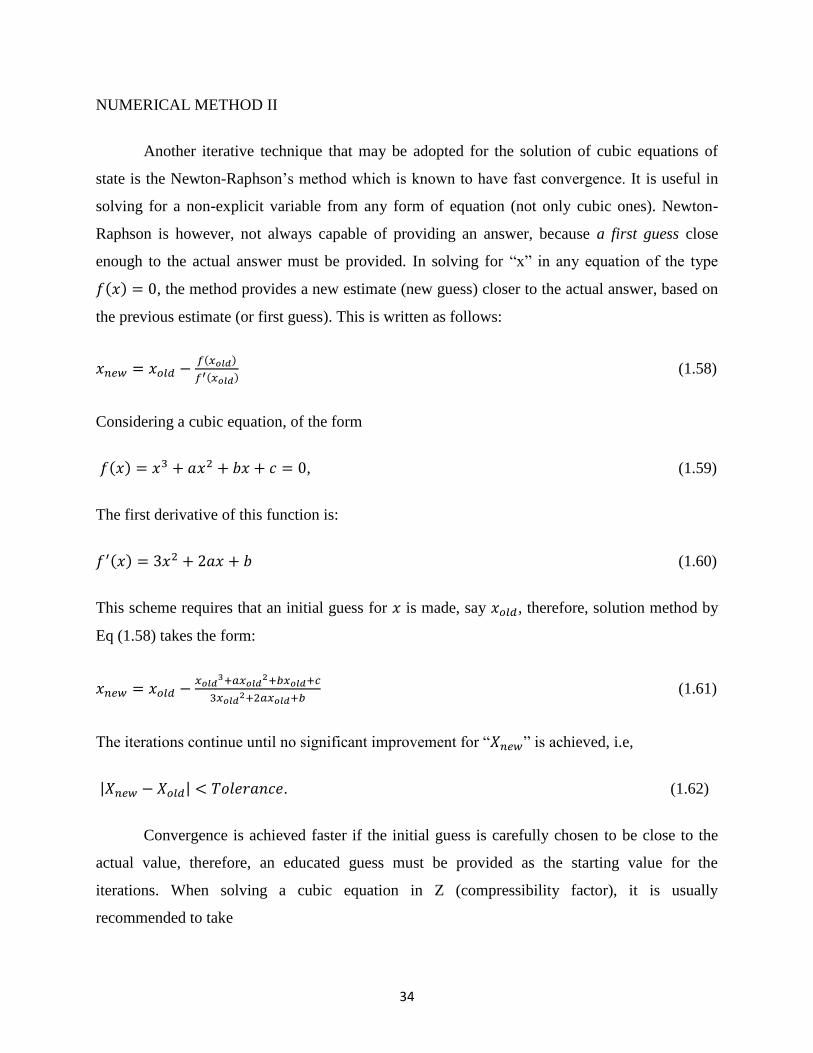
NUMERICAL METHOD II
Another iterative technique that may be adopted for the solution of cubic equations of
state is the Newton-Raphson’s method which is known to have fast convergence. It is useful in
solving for a non-explicit variable from any form of equation (not only cubic ones). Newton-
Raphson is however, not always capable of providing an answer, because a first guess close
enough to the actual answer must be provided. In solving for “x” in any equation of the type
𝑓(𝑥) = 0, the method provides a new estimate (new guess) closer to the actual answer, based on
the previous estimate (or first guess). This is written as follows:
𝑥𝑛𝑒𝑤 = 𝑥𝑜𝑙𝑑 −𝑓(𝑥𝑜𝑙𝑑)
𝑓′(𝑥𝑜𝑙𝑑) (1.58)
Considering a cubic equation, of the form
𝑓(𝑥) = 𝑥3 + 𝑎𝑥2 + 𝑏𝑥 + 𝑐 = 0, (1.59)
The first derivative of this function is:
𝑓′(𝑥) = 3𝑥2 + 2𝑎𝑥 + 𝑏 (1.60)
This scheme requires that an initial guess for 𝑥 is made, say 𝑥𝑜𝑙𝑑, therefore, solution method by
Eq (1.58) takes the form:
𝑥𝑛𝑒𝑤 = 𝑥𝑜𝑙𝑑 −𝑥𝑜𝑙𝑑
3+𝑎𝑥𝑜𝑙𝑑2+𝑏𝑥𝑜𝑙𝑑+𝑐
3𝑥𝑜𝑙𝑑2+2𝑎𝑥𝑜𝑙𝑑+𝑏
(1.61)
The iterations continue until no significant improvement for “𝑋𝑛𝑒𝑤” is achieved, i.e,
|𝑋𝑛𝑒𝑤 − 𝑋𝑜𝑙𝑑| < 𝑇𝑜𝑙𝑒𝑟𝑎𝑛𝑐𝑒. (1.62)
Convergence is achieved faster if the initial guess is carefully chosen to be close to the
actual value, therefore, an educated guess must be provided as the starting value for the
iterations. When solving a cubic equation in Z (compressibility factor), it is usually
recommended to take
35
𝑍 = 𝑏𝑃 𝑅𝑇⁄ (1.63)
as the starting guess for the compressibility of the liquid phase and
𝑍 = 1 (1.64)
for the vapor root.
1.4.3 Semi-Analytical Scheme
In this method one root of the cubic equation is obtained by the numerical method
discussed earlier. The other two real roots, if they exist, can then be obtained by the semi-
analytical scheme. By using the relationships given before, with the value ‘𝑥1’ as the root already
known, the other two roots are calculated by solving the system of equations:
𝑥2 + 𝑥3 = −𝑎 − 𝑥1 (1.65)
𝑥2𝑥3 = − 𝑐 𝑥1⁄ (1.66)
which leads to a quadratic expression.
This procedure can be reduced to the following steps:
1. Let 𝑥3 + 𝑎𝑥2 + 𝑏𝑥 + 𝑐 = 0 be the original cubic polynomial and “𝑊” the root which is
already known (𝑥1 − 𝑊).
Then, we may factorize such a cubic expression as:
(𝑥1 − 𝑊)(𝑥2 + 𝐹𝑥 + 𝐺) = 0 (1.67)
where:
𝐹 = 𝑎 + 𝑊 (1.68)

36
𝐺 = − 𝑐 𝑊⁄ (1.69)
2. Solve for x2, x3 by using the quadratic expression formulae,
𝑥1 = 𝑊 (1.70)
𝑥2 =−𝐹+√𝐹2−4𝐺
2 (1.71)
𝑥3 =−𝐹−√𝐹2−4𝐺
2 (1.72)
1.4.4 Graphical Scheme
By using graph sheets, sophisticated calculators which can make plots or spreadsheets in
computers, make a plot of the relation using a wide range of possible 𝑥 values to solve the
relation 𝑓(𝑥) = 𝑥3 + 𝑎𝑥2 + 𝑏𝑥 + 𝑐 = 0. The plot would have a semblance to what is shown in
the figure below cutting the horizontal, (𝑥 = 0) axis in three places. The points where the curve
intersects the horizontal axis are the roots of the relation:
Figure 1.8 Graphical method of finding roots of cubic polynomials
𝑓(𝑥)
(𝑥)
0
37
1.5 Some Shortcomings of Cubic Equations of State
While cubic equations of state are useful, they have some shortcomings. The most
prominent of these shortcomings are listed below:
i. They require accurate description of all the components in a mixture for best predictions
of PVT properties.
ii. They are computationally expensive for mixtures with large number of constituents.
iii. Most are biased to a fluid property, i.e. either gas or liquid property are better described
and not both.
iv. Flexibility at all regions of the phase diagram is lacking, so all cubic EOSs fail in the
immediate neighborhood of the critical point.
v. They have very weak, almost inexistent theoretical backgrounds. Hence the
understanding of the physics of fluid properties from a macroscopic perspective is not
well defined.

38
1.6 Scope of Work
In scope, this work thoroughly reviews the two parameter van der Waals, Redlich-Kwong’s,
Soave-Redlich Kwong’s and Peng-Robinson’s two-parameter and the Patel-Teja’s three
parameter Cubic equations of State (CEOS). A New three parameter Cubic Equation of state is
then developed and validated using experimental data from literature. The performance of the
New equation in predicting gas compressibility factors for the gas phase and liquid densities for
the liquid phase is compared to prediction performances by the Peng-Robinson and Patel-Teja’s
equations of state. Prediction of liquid density values are of interest because it’s prediction is the
major known weakness of most cubic equations of state.

39
1.7 OBJECTIVES OF STUDY
Despite the extensive and painstaking research that has been spent on equation of state
development and modifications, the best in the industry today, (Patel-Teja’s EOS) still falls short
from the high performance required to narrow the gap between predicted and experimental
results for the parameters of interest. This informs the need for a new EOS that would
significantly improve accuracy without compromising on the simplicity for which cubic EOSs
are famous.
The main goal sought with the new equation, is to provide a simple equation of state model,
which is versatile, flexible, and more accurate over a wider range of liquid density than does the
existing ones. Other design objectives are:
1. Ability to estimate thermodynamic properties within limits of experimental uncertainty
without need for arbitrary corrections.
2. The parameters should be expressible in terms of the critical properties and the acentric
factor.
3. The mixing rules should not employ more than a single binary interaction parameter,
which should be independent of pressure, temperature and composition.
4. The equation of state must obey the Maxwell criterion of equal Gibbs energies for
saturated liquid and saturated vapor.
5. The equation should provide reasonable accuracy near the critical point, particularly for
calculations of liquid density.
6. Most importantly, the resultant equation must significantly reduce the bias between
experimentally determined thermodynamic data and that obtained by other popular (PR
and PT) equations of state.
40
CHAPTER TWO
2.0 REVIEW OF PERTINENT LITERATURE
2.1 Theoretical Background: Van der Waal’s (vdW) (1873) was the first equation capable
of predicting vapor-liquid coexistence. This break-through hinges on the then, novel assumption
that, molecules themselves, occupy a finite volume (co-volume) of the total volume occupied by
the fluid.
The vdW EOS formed the basic foundation over which most other researchers built their
framework by either modifying the attractive, repulsive or both terms of the original van der
Waals contributors to pressure. The Redlich-Kwong Equation of state (RK), (1949) improved the
accuracy of the van der Waals EOS by introducing temperature-dependence for the attractive
term. Soave (1972) and Peng and Robinson (1976) proposed additional modifications to more
accurately predict the vapor pressure, liquid density, and equilibria ratios.
2.2 Cubic Equations of State (CEOS)
Equations based on the attraction term modification of the original vdW EOS are referred
to as the van der Waals family of EOS. They can be shown to be cubic polynomials when
expressed in terms of volume or compressibility factors and are therefore often called cubic
equations of state (CEOS). They are sufficiently accurate for simple fluids (i. e. molecules for
which the most important intermolecular forces are repulsion and dispersion (van der Waals
attractions), together with weak electrostatic forces due to dipoles, quadrupoles, etc.).A few of
the popular cubic equations of state (CEOS) are discussed hereunder starting with van der Waals
EOS:
2.2.1 Popular CEOS in Reservoir Engineering Calculations:
Quite a number of cubic equations of state are popular with reservoir engineering
calculations. There are two-, three and even four parameter cubic equations of state. This
discussion focusses on just the two- and three-parameter CEOSs.

41
2.2.1(a) Two-Parameter Cubic Equations of State:
Two parameter equations of state have just the original two (𝑎 and 𝑏) parameters of the
vdW original EOS. Their derivation is essentially empirical-neither direct nor rigorous. The
driving factor was in reproducing the experimental compressibility factor which for pure
substances ranges from about 0.24 to 0.31 or the value of parameter 𝑏 in such a way that
0.24𝑉𝑐 ≤ 𝑏 ≤ 0.28𝑉𝑐. The functional form of a with respect to the critical temperature and
pressure is generally empirically chosen to give the best fit at moderate pressures for most
relatively non-polar gasses. (Reif-Acherman, 2008).
2.2.1(a).1 van der Waal’s (vdW) EOS (1873):
The existence of a simple, closed, analytic equation describing the state of a material is
limited to an ideal gas. Various interactions, each modeled separately through different theories,
whose validity is confined to specific temperature, pressure or density conditions is required for
phase behavior modeling outside the realm for which ideal gases exist. The equation of state
presented by Johannes Diderick van der Waals is credited as the first successful attempt in real
gas behavior modeling. In its simple form, the van der Waals (vdW) EOS is stated as follows:
(𝑃 +𝑎
𝑉2) (𝑉 − 𝑏) = 𝑅𝑇 (2.1)
Where, P is the pressure of the fluid, V is the molar volume of the container containing the fluid,
(𝑓𝑡3 𝑚𝑜𝑙𝑒)⁄ , (𝑎 and 𝑏) are substance specific constants. In Equation (2.1) a, is the attraction
parameter which measures the attractive forces between the molecules, and 𝑏 called co-volume,
is a parameter which represents the volume occupied by the molecules. It is a measure of the size
of the molecules and its value is the volume of one mole of the atoms or molecules. Since there
are only two parameters, ‘𝑎 𝑎𝑛𝑑 𝑏′, in the vdW EOS, it is classified as a two-parameter EOS.
Expressed in pressure explicit form, the vdW EOS is written as:
𝑃 = 𝑅𝑇
(𝑉−𝑏) −
𝑎
𝑉2 (2.2)

42
In the pressure explicit form of van der Waals equation, shown as Eq. (2.2), the first term
makes the compressibility factor larger than the ideal gas value to account for repulsive forces
among molecules. The second term makes the compressibility factor smaller due to forces of
attraction. In effect, the two forces compete in their effects on the compressibility factor and
depending on state conditions of pressure and density, one term would dominate. In the low
density limit, the van der Waals equation collapses to the ideal gas law, while it approximates the
hard sphere equation of state in the high temperature limit.
The vdW equation is regarded as the ideal gas law improved due to two independent reasons:
i. The molecules have volume which is significant enough to be accounted for when
compared to gas volume. So, 𝑉 cannot be too little, less than some constant, ′𝑏′ , called
co-volume, which represents the volume of the molecules. So instead of 𝑉 in the ideal
gas law, (𝑉 − 𝑏) is used instead.
ii. Unlike with ideal gases, real gas molecules attract others within a distance of several
molecules’ radii. Though this makes no effect inside the material, it causes surface
materials to be attracted into the material, diminishing the pressure on the outer shell
(which is used in the ideal gas law). Therefore, the actual pressure is less than the ideal
gas pressure by some constant which vdW expressed as 𝑎
𝑉2.
The van der Waals equation of state approaches the ideal gas law 𝑃𝑉 = 𝑛𝑅𝑇 as the
values of the constants (𝑎 𝑎𝑛𝑑 𝑏) approach zero.
Considering the vdW’s EOS expressed in pressure-explicit form, Eq. (2.2), the repulsive term is
𝑅𝑇
(𝑉−𝑏) and the attractive term is
𝑎
𝑉2. Sadus (1994) was the first to point out that pressure is a sum
of two components, pressure due to attraction and pressure due to repulsion, which is the hard
sphere term; that is
𝑃 = 𝑃𝑟𝑒𝑝𝑢𝑙𝑠𝑖𝑜𝑛 + 𝑃𝑎𝑡𝑡𝑟𝑎𝑐𝑡𝑖𝑜𝑛 (2.3)
The following can be inferred from Eq. (2.2):
1. At low pressures and large volumes, the co-volume, 𝑏 becomes very insignificant in
comparison to the molar volume of the container, 𝑉, that is, 𝑉 ≫ 𝑏 such that 𝑉 − 𝑏 ≅ 𝑉.

43
Consequently, the attraction forces term becomes insignificant or negligible, causing the
van der Waal’s equation, Eq. (2.2) to revert to the ideal gas equation: 𝑃 = 𝑅𝑇 𝑉⁄ .
2. At infinitely high pressures, that is, as 𝑃 → ∞, the molar volume V becomes very small
asymptotically approaching the value 𝑏 , which is the actual molecular volume, but never
diminishing to zero.
When dealing with hydrocarbon systems, the practice of expressing pressure as the sum of
two terms (repulsive and attractive) has gained wide popularity since its introduction in 1873 by
van der Waals. All equations of state that can be expressed in two-terms in pressure explicit form
(𝑖. 𝑒. 𝑃 = 𝑃𝑎𝑡𝑡𝑟 + 𝑃𝑟𝑒𝑝) are referred to as van der Waal-type EOSs.
Expressed in molar volume, vdW is:
𝑉3 − (𝑏 +𝑅𝑇
𝑃) 𝑉2 + (
𝑎
𝑃) 𝑉 − (
𝑎𝑏
𝑃) = 0 (2.4)
At the critical point, the three roots of the cubic equation are identical. Thus, if 𝑉𝑐 represents the
critical volume, then at the critical point:
(𝑉 − 𝑉𝑐)3 = 𝑉3 − 3𝑉𝑐𝑉2 + 3𝑉𝑐2𝑉 − 𝑉𝑐
3 = 0 (2.5)
By comparing equations (2.4) and (2.5), it can be shown that:
𝑎 = 3𝑃𝑐𝑉𝑐3 (2.6)
𝑏 = 𝑉𝑐 3⁄ (2.7)
𝑎𝑛𝑑 𝑅 =8𝑃𝑐𝑉𝑐
3𝑇𝑐 (2.8)
𝑉𝑐 is the molar volume at the critical point.
In terms of the compressibility factor, the van der Waals EOS is written as:
𝑍3 − (1 +𝑏𝑃
𝑅𝑇) 𝑍2 +
𝑎𝑃
(𝑅𝑇)2 𝑍 −𝑎𝑏𝑃2
(𝑅𝑇)3 = 0 (2.9)
or in terms of reduced quantities (compressibility factor form):
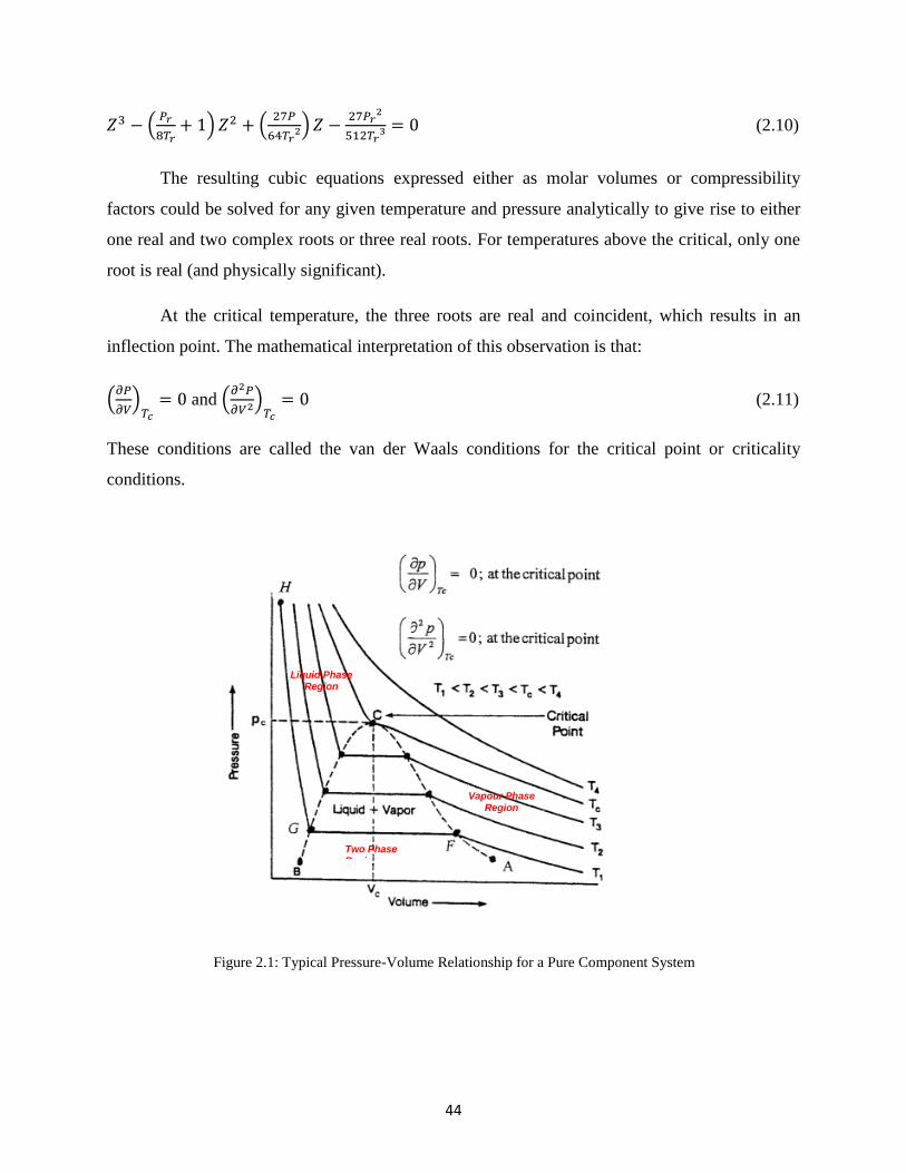
44
𝑍3 − (𝑃𝑟
8𝑇𝑟+ 1) 𝑍2 + (
27𝑃
64𝑇𝑟2) 𝑍 −
27𝑃𝑟2
512𝑇𝑟3 = 0 (2.10)
The resulting cubic equations expressed either as molar volumes or compressibility
factors could be solved for any given temperature and pressure analytically to give rise to either
one real and two complex roots or three real roots. For temperatures above the critical, only one
root is real (and physically significant).
At the critical temperature, the three roots are real and coincident, which results in an
inflection point. The mathematical interpretation of this observation is that:
(𝜕𝑃
𝜕𝑉)
𝑇𝑐
= 0 and (𝜕2𝑃
𝜕𝑉2)𝑇𝑐
= 0 (2.11)
These conditions are called the van der Waals conditions for the critical point or criticality
conditions.
Figure 2.1: Typical Pressure-Volume Relationship for a Pure Component System
Two Phase Region
Liquid Phase Region
Vapour Phase Region

45
vdW (1873) showed that an EOS can represent the phase behavior of the fluid, both in
the two-phase envelope (i.e., inside the binodal curve), and outside the binodal curve. For
temperatures greater than the critical temperature, (i.e. 𝑇 > 𝑇𝑐), the pressure versus volume
isotherms do not look much different from that of the ideal gas. However, at the critical
temperature, 𝑇 = 𝑇𝑐, the isotherm develops an inflection point at 𝑃𝑐 =𝑎
27𝑏2, and 𝑉𝑐 = 3𝑏. The
points 𝑃𝑐, 𝑇𝑐 and 𝑉𝑐 define the critical point of the gas liquid transition. Usually, the pressure,
temperature and volume at the critical point, are known and by applying Eq.(2.11) to Eq.(2.2) it
is possible to calculate the empirical constants a and b:
Differentiating Eq. (2.2) with respect to the volume at the critical point results in:
[𝜕𝑃
𝜕𝑉]
𝑇𝑐
= −𝑅𝑇𝑐
(𝑉−𝑏)2 +2𝑎
𝑉𝑐3 = 0 (2.12)
[𝜕2𝑃
𝜕𝑉2]𝑇𝑐
=2𝑅𝑇𝑐
(𝑉𝑐−𝑏)3 −6𝑎
𝑉𝑐4 = 0 (2.13)
These two equations can be solved simultaneously to give the parameters 𝑎 and 𝑏 as follows:
𝑎 =27𝑅2𝑇𝑐
2
64𝑃𝑐 (2.14)
𝑏 =𝑅𝑇𝑐
8𝑃𝑐 (2.15)
By applying Eq.(2.2) at the critical point, that is, by setting T = Tc , P = Pc and V = Vc,
and substituting for a and b from Eqs. (2.14) and (2.15), respectively, gives:
𝑃𝑐 =3𝑅𝑇𝑐
8𝑉𝑐 (2.16)
The Z-factor at the critical state for a van der Waal gas is given as:
Zc =𝑃𝑐𝑉𝑐
𝑅𝑇𝑐=
3
8= 0.375 (2.17)
For generality and ease of comparison with other EOSs, Eqs. (2.14) and (2.15) are written in the
form:
𝑎 = Ω𝑎𝑅2𝑇𝑐
2
𝑃𝑐 (2.18)
and 𝑏 = Ω𝑏𝑅𝑇𝑐
𝑃𝑐. (2.19)
which for vdW’s EOS, has the following values for Ω𝑎 and Ω𝑏:
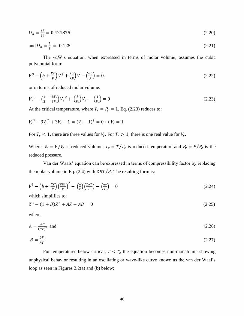
46
Ω𝑎 =27
64= 0.421875 (2.20)
and Ω𝑏 =1
8 = 0.125 (2.21)
The vdW’s equation, when expressed in terms of molar volume, assumes the cubic
polynomial form:
𝑉3 − (𝑏 +𝑅𝑇
𝑃) 𝑉2 + (
𝑎
𝑃) 𝑉 − (
𝑎𝑏
𝑃) = 0. (2.22)
or in terms of reduced molar volume:
𝑉𝑟3 − (
1
3+
8𝑇𝑟
3𝑃𝑟) 𝑉𝑟
2 + (3
𝑃𝑟) 𝑉𝑟 − (
1
𝑃𝑟) = 0 (2.23)
At the critical temperature, where 𝑇𝑟 = 𝑃𝑟 = 1, Eq. (2.23) reduces to:
𝑉𝑟3 − 3𝑉𝑟
2 + 3𝑉𝑟 − 1 = (𝑉𝑟 − 1)3 = 0 ↔ 𝑉𝑟 = 1
For 𝑇𝑟 < 1, there are three values for 𝑉𝑟. For 𝑇𝑟 > 1, there is one real value for 𝑉𝑟.
Where, 𝑉𝑟 = 𝑉 𝑉𝑐⁄ is reduced volume; 𝑇𝑟 = 𝑇 𝑇𝑐⁄ is reduced temperature and 𝑃𝑟 = 𝑃 𝑃𝑐⁄ is the
reduced pressure.
Van der Waals’ equation can be expressed in terms of compressibility factor by replacing
the molar volume in Eq. (2.4) with 𝑍𝑅𝑇 𝑃⁄ . The resulting form is:
𝑉3 − (𝑏 + 𝑅𝑇
𝑃) (
𝑍𝑅𝑇
𝑃)
2+ (
𝑎
𝑃) (
𝑍𝑅𝑇
𝑃) − (
𝑎𝑏
𝑃) = 0 (2.24)
which simplifies to:
𝑍3 − (1 + 𝐵)𝑍2 + 𝐴𝑍 − 𝐴𝐵 = 0 (2.25)
where,
𝐴 =𝑎𝑃
(𝑅𝑇)2 and (2.26)
𝐵 =𝑏𝑃
𝑅𝑇 (2.27)
For temperatures below critical, 𝑇 < 𝑇𝑐 the equation becomes non-monatomic showing
unphysical behavior resulting in an oscillating or wave-like curve known as the van der Waal’s
loop as seen in Figures 2.2(a) and (b) below:
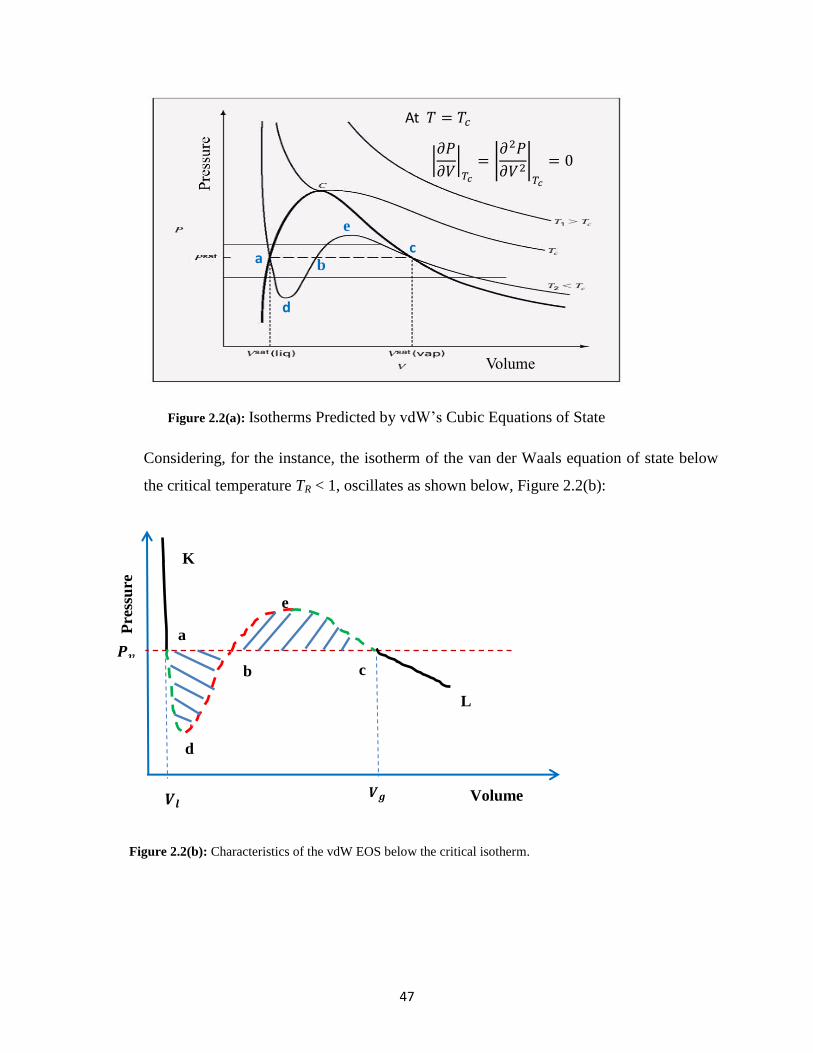
47
Figure 2.2(a): Isotherms Predicted by vdW’s Cubic Equations of State
Considering, for the instance, the isotherm of the van der Waals equation of state below
the critical temperature TR < 1, oscillates as shown below, Figure 2.2(b):
Figure 2.2(b): Characteristics of the vdW EOS below the critical isotherm.
a
b
a
c
a
e
c
a
d
𝑽𝒍 𝑽𝒈
Pre
ssu
re
Volume
𝑷𝒗
K
L
At 𝑇 = 𝑇𝑐
|𝜕𝑃
𝜕𝑉|
𝑇𝑐
= |𝜕2𝑃
𝜕𝑉2|
𝑇𝑐
= 0
a b c
d
e
Volume

48
The pressure-volume plot of Figures 2.2(a) and 2.2(b) above, show that below the critical
isotherm, the vdW EOS gives rise to three possible roots for any given pressure at volumes
corresponding to points 𝑎, 𝑏 and 𝑐. The intermediate root (𝑏) is discarded as having no
theoretical significance whereas the lowest (𝑎) and highest (𝑐) values are assigned to the liquid
and vapor phases respectively (Danesh, 1998).
From Figure 2.2b, along the dashed portion, shown in red, of the isotherm the curve is
linearly unstable since (𝜕𝑃 𝜕𝑉⁄ )𝑇,𝑁 > 0. (𝑁 is the number of particles). The van der Waals
equation fails to describe real substances in this region. This is because the equation always
assumes that the fluid is uniform while between a and c on the isotherm it becomes more stable
to be a coexistence of two different phases, a denser phase (normally called liquid) and a sparser
phase (normally called gas).
The loops between 𝑎 𝑎𝑛𝑑 𝑐 may be eliminated using the Maxwell construction, named
after the founder, James Clerk Maxwell (1875). In this construction, the oscillating portion is
replaced by a horizontal line (isobar) positioned so that the areas of the two hatched regions
above and below the line (which contribute to ∮ 𝑉𝑑𝑃 with opposite signs) are equal. This is
known as the Maxwell’s equal areas rule. The flat line portion of the isotherm now connects the
liquid and vapor phases that coexist at equilibrium. Thus, the physical P-V curve is given by
(𝐾 − 𝑎 − 𝑐 − 𝐿).
The portions a–d and c–e are interpreted as metastable states of super-heated liquid and
super-cooled vapor respectively. As a function of the extensive variable, V, there is a region
(𝑏𝑒𝑡𝑤𝑒𝑒𝑛 𝑉𝑙 𝑎𝑛𝑑 𝑉𝑔) of phase coexistence. The densities of the extensive variables of the two
phases in equilibrium are discontinuous across the transition. According to thermodynamic
principles, for two systems in contact to be in equilibrium, there must be mechanical, thermal
and chemical equilibrium, such that;
𝑃𝑔 = 𝑃𝑙 , 𝑇𝑔 = 𝑇𝑙 𝑎𝑛𝑑 𝜇𝑔 = 𝜇𝑙, respectively. (2.28)
The chemical potential equality of Eq. (2.28) was proposed by Maxwell (1875).
Chemical potential is a function of pressure and temperature such that at two phase

49
coexistence:𝜇𝑔(𝑇, 𝑃) = 𝜇𝑙(𝑇, 𝑃). This provides a single constraint on the two variables
temperature, 𝑇 and pressure, 𝑃, i.e., two phase coexistence occurs along a line in the 𝑇, 𝑃 plane.
The equal area rule can be expressed as:
𝑃𝑣(𝑉𝑔 − 𝑉𝑙) = ∫ 𝑃𝑑𝑉𝑉𝑔
𝑉𝑙 (2.29)
Where, 𝑉𝑙 and 𝑉𝑔 are the volumes of the pure liquid and pure gas phases respectively, marked as
𝑎 and 𝑐, respectively, in Figures, 2.2(a) and 2.2(b). The sum of these volumes equals the total
volume.
On the isotherm shown in Figure 2.2b, points 𝑎 and 𝑐 are the only pair of points which
satisfy the three equilibrium conditions of Eq. (2.28). It follows that systems with volumes
intermediate between these two points will consist of a mixture of the pure liquid and gas with
specific volumes equal to the pure liquid and gas phases at points 𝑎 and 𝑐.
In spite of the remarkable contributions of the van der Waals equation of state and its
superior performance over the ideal gas equation, the agreement with experimental data is
limited to conditions where the liquid forms. As Nasrifar, et al. (2006) established, it performs
poorly with respect to the liquid phase and thus, cannot be used to accurately calculate vapor-
liquid equilibria. One of its principal drawbacks is that the maximum pressure for which the
equation is applicable is still far below the normal range of reservoir pressures. (Valderrama,
2003).
Eq. (2.17) suggests that the vdW EOS predicts a common critical compressibility factor,
Zc value of 0.375 irrespective of the substance. This is larger than the typical 0.22~0.30 range
obtained by experimental studies. As a consequence, if the critical pressure and the temperature
are used to calculate the parameters, the critical volume would be over-predicted by the vdW
EOS to a tune of roughly 30%. The major criticism of the vdW EOS is that no account is taken
of the possibility that parameters a and /or b can depend on temperature.
50
2.2.1(a).1 The Theorem of Corresponding States
van der Waals (1873) established the relationship between the reduced temperature, 𝑇𝑟,
the reduced pressure, 𝑃𝑟, and the compressibility factor.
𝑍 = 𝑍(𝑃𝑟 , 𝑇𝑟) (2.30)
Fig. 2.2 shows Z as a function of 𝑃𝑟 for 10 substances with 𝑇𝑟 as the parameter. Excellent
quantitative agreement is achieved. This unique relationship, in the behavior of all pure
compounds, known as the law of corresponding states is applicable to a homologous series of
compound. A brief statement of this law is “the ratio of the value of any intensive property to the
value of that property at the critical state is related to the ratios of the prevailing absolute
temperature and pressure to the critical temperature and pressure by the same function for all
similar substances.” Validity of this relationship would make it necessary to only investigate in
detail the behavior of a single substance of a homologous series, and then determine the
volumetric properties of each of the other members from knowledge of its critical pressure,
temperature and specific volume. The ratio of the value of an intensive property at a given state
to its value at the critical state is called the reduced value of the property.
The three critical constants 𝑃𝑐 , 𝑉𝑐 𝑎𝑛𝑑 𝑇𝑐 can be expressed in terms of the one universal
and two specific constants of van der Waals equation, 𝑅, 𝑎 𝑎𝑛𝑑 𝑏. By introducing the ratios
𝜋 = 𝑃 𝑃𝑐⁄ , 𝜑 = 𝑉 𝑉𝑐⁄ and 𝜏 = 𝑇 𝑇𝑐⁄ van der Waals equation can be expressed in the universal
form:
(𝜋 +3
𝜑2) (3𝜑 − 1) = 8𝜏 (2.31)

51
Figure 2.3: Experimental Data and Generalized z-factor Chart
(Source: Moran and Shapiro, 2000)
The two-parameter corresponding states principle, though sufficient for simple fluid
calculations fails when applied to complex gases. It is not sufficient by itself for dealing with
gases in which the molecules have strong dipolar moments and/or non-spherical force fields. In
these cases a third parameter is introduced to give three parameter corresponding principles. Two
approaches have been followed to choose the third parameter. In the first, the critical
compressibility factor has been added, so that the resulting three parameter corresponding
principle is:
𝑍 = 𝑍(𝑃𝑟 , 𝑇𝑟 , 𝑍𝑐) (2.32)
This approach provides significant improvement in accuracy, since now the critical
compressibility factor can be accurately adjusted in a three-parameter EOS.
The second approach adds the acentric factor, 𝜔 which gives an indication of the deviation from
spherical symmetry in a molecule.
52
2.2.1(a).2 Redlich Kwong (RK) EOS (1949):
The empirical, algebraic equation, of Redlich and Kwong (1949) proved to be generally
more accurate than the van der Waal’s Eos and the ideal gas equation at temperatures above the
critical temperature. Redlich and Kwong demonstrated that, by replacing the attraction term of
the vdW EOS with a generalized temperature dependent term, the resulting EOS could
considerably improve the prediction of the volumetric and physical properties of the vapor phase.
The functional form of 𝑎 with respect to the critical temperature and pressure is empirically
chosen to give the best fit at moderate pressures for most relatively non-polar gases. (Reif-
Acherman, 2008). However, it performs poorly with respect to the liquid phase and therefore,
cannot be used to accurately calculate vapor–liquid equilibria.
Redlich and Kwong’s EOS has the following form:
𝑃 = 𝑅𝑇
𝑉−𝑏−
𝑎
𝑉 (𝑉+𝑏)𝑇0.5 (2.33)
where, as is the case with the vdW EOS, 𝑎 is a constant that corrects for attractive potential of
molecules and 𝑏 is a constant that corrects for volume. These constants can be calculated from
the critical point data of the gas:
𝑎 = 0.42747𝑅2𝑇𝑐
2.5
𝑃𝑐 (2.34)
𝑏 = 0.08664 𝑅𝑇𝑐
𝑃𝑐 (2.35)
Where, 𝑇𝑐 and 𝑃𝑐 are the critical temperature pressure, respectively.
The RK EOS is adequate for calculation of gas phase properties when the ratio of the
pressure to the critical pressure (reduced pressure) is less than about one-half of the ratio of the
temperature to the critical temperature (reduced temperature).
𝑃
𝑃𝑐<
𝑇
2𝑇𝑐 (2.36)
𝑜𝑟 𝑃𝑟 <1
2𝑇𝑟 (2.37)
When expressed in terms of compressibility factor, the RK EOS is written as:
𝑍3 − 𝑍2 + (𝐴 − 𝐵 − 𝐵2)𝑍 − 𝐴𝐵 = 0 (2.38)
53
With:
𝐴 = 𝑎𝑃
𝑅2𝑇2.5 (2.39)
𝐵 = 𝑏𝑃
𝑅𝑇 (2.40)
The Redlich-Kwong equation of state did not have a strong theoretical background but
was quite successful for the calculation of the properties of gas mixtures. It should also be
mentioned that, when Redlich and Kwong proposed their equation of state, they were interested
in developing a good equation for gases only. The original paper by Redlich and Kwong did not
contain any application of the developed EOS to liquids. Therefore, it was still not adequate for
the modeling of both gas and liquid phases.
The fugacity coefficient of a gas can be estimated using thee the RK EOS as:
ln ∅ = ∫𝑧−1
𝑃
𝑃
0𝑑𝑝 = 𝑧 − 1 − 𝑙𝑛(𝑧 − 𝐵𝑃) −
𝐴2
𝐵𝑙𝑛 (1 +
𝐵𝑃
𝑧) (2.41)
[Source: http://energy.sdsu.edu/testhome/Test/solve/basics/tables/tablesRG/zLK.html]
The RK EOS unarguably, does a much better job than the original van der Waals EOS,
but still predicts a slightly high compressibility factor at the critical state of Z=1/3. The critical
compressibility factor, 𝑍𝑐 of 0.333, suggests an improvement over the vdW’s EOS which had a
𝑍𝑐 = 0.375. In reality, the critical compressibility factor is not constant for different fluids and is
generally smaller than 0.3. For example, water has a critical compressibility of about 0.23, and
that of carbon dioxide is 0.27. The value ranges between about 0.24𝑉𝑐 and 0.29𝑉𝑐. [Redlich
(1975)].
The poor match of the van der Waals EOS at the critical point explains why the RK EOS
is not as popular toady. Moreover, the accuracy of the RK EOS in liquid volume and hence,
density predictions, are unreasonable.

54
2.2.1(a).3 Soave-Redlich-Kwong (SRK) EOS (1972): In 1972, Soave improved on the RK
EOS by replacing the 1
√𝑇 term of the Redlich Kwong EOS with a more general temperature
dependent term, 𝑎(𝑇). The resulting EOS, called Soave-Redlich-Kwong (SRK) EOS, which has
the form of Eq. (2.39) below, enabled representation of vapor pressure of a wide class of
substances.
𝑃 = 𝑅𝑇
𝑉−𝑏−
𝑎(𝑇)
𝑉(𝑉+𝑏) (2.42)
Where, 𝑏 = 0.08664 𝑅𝑇𝑐
𝑃𝑐 (2.43)
and 𝑎(𝑇) = 0.42747𝑅2𝑇𝑐
2
𝑃𝑐 𝛼(𝑇) (2.44)
Soave proposed a simple form for 𝛼 as a function of reduced temperature, 𝑇𝑟 and acentric
factor, 𝜔, shown as Eq. (2.42) below. The acentric factor is a conceptual number introduced by
Kenneth Pitzer in 1955. Originally, Pitzer’s acentric factor, 𝜔, represents a measure of the
acentricity or nonsphericity of a molecule; for spherical molecules, 𝜔 = 0. It is used, now, for
the complexity of a molecule with respect to both the geometry and polarity.
𝛼(𝑇) = 1 + 𝑚 [1 − (𝑇
𝑇𝑐)
0.5
]2
(2.45)
𝑚 = 0.48508 + 1.55171𝜔 − 0.1561𝜔2 (2.46)
𝜔 is the acentric factor.
Expressed in terms of molar volume, the SRK EOS has the form:
𝑉3 − [ 𝑅𝑇
𝑃] 𝑉2 + [
𝑎𝛼
𝑃−
𝑏𝑅𝑇
𝑃− 𝑏2
] 𝑉 − [(𝑎𝛼)𝑏
𝑃] = 0 (2.47)
At the critical point,
(𝑣 − 𝑣𝑐)3 = 0 (2.48)
Expanding,
𝑣3 − 3𝑣𝑐𝑣2 + 3𝑣𝑐2𝑣 − 𝑣𝑐
3 = 0 (2.49)
55
By imposing the condition that:
(𝑍 − 𝑍𝑐)3 = 0 (2.50)
and by expanding:
𝑍3 − 3𝑍𝑐𝑍2 + 3𝑍𝑐2𝑍 − 𝑍𝑐
3 = 0 (2.51)
The SRK EOS (Eq. (2.43)) can be expressed in terms of compressibility factor by
replacing the molar volume, V, by (ZRT/P) and rearranging to give:
𝑍3 − 𝑍2 + (𝐴 − 𝐵 − 𝐵2)𝑍 − 𝐴𝐵 = 0 (2.52)
With
𝐴 = (𝑎𝛼)𝑃
(𝑅𝑇)2 (2.53)
and 𝐵 = 𝑏𝑃
𝑅𝑇 (2.54)
By comparing coefficients between Eqs. (2.51) and (2.52):
−3𝑍𝑐 = −1 : Coefficient of 𝑍2 terms, implying that
𝑍𝑐 =1
3= 0.333 (2.55)
The SRK EOS is quite capable of predicting vapor-liquid equilibria, but it does not
provide reliable liquid density (Danesh, 1998).
56
2.2.1(a).4 Peng Robinsons (PR) EOS (1976):
With a goal to improve ability of the Equation of state to predict liquid densities and other
reservoir fluid properties, particularly in the vicinity of the critical region, as a basis, they first
proposed the form:
𝑃 =𝑅𝑇
𝑉−𝑏−
𝑎𝛼
(𝑉+𝑏)2−𝑐𝑏2 (2.56)
where a, b and 𝛼 have the same significance as they have in the SRK model, and the parameter c
is a whole number optimized by analyzing the values of the terms 𝑍𝑐 and 𝑏 𝑉𝑐⁄ as obtained from
the equation. It is generally accepted that 𝑍𝑐 should be close to 0.28 and 𝑏 𝑉𝑐⁄ should be
approximately 0.26. An optimized value of 𝑐 = 2 gives the final form of the PR EOS as:
𝑃 =𝑅𝑇
(𝑉−𝑏)−
𝑎𝑐𝛼(𝑇𝑟,𝜔)
𝑉(𝑉+𝑏)+𝑏(𝑉−𝑏) (2.57)
or
𝑍 =𝑉
𝑉−𝑏−
𝑎𝑐𝛼(𝑇𝑟,𝜔)𝑉
𝑅𝑇[𝑉(𝑉+𝑏)+𝑉(𝑉−𝑏)] (2.58)
where,
𝑎𝑐 = 0.45724𝑅𝑇𝑐
2.5
𝑃𝑐 (2.59)
𝑏 = 0.07780𝑅𝑇𝑐
𝑃𝑐 (2.60)
𝛼(𝑇𝑟 , 𝜔) = [1 + 𝑚(1 − 𝑇𝑟0.5)]
2 (2.61)
𝑚 = 0.37464 − 1.54226𝜔 − 0.26992𝜔2 (2.62)
The correlation was later modified to improve predictions for heavier components 𝑓𝑜𝑟 𝜔 >
0.49:
𝑚 = 0.3796 + 1.485𝜔 − 0.1644𝜔2 + 0.01667𝜔3 (2.63)

57
Expressed in terms of compressibility factor, the PR EOS is:
𝑍3 + (𝐵 − 1)𝑍2 + (𝐴 − 3𝐵2 − 2𝐵)𝑍 + (𝐵2 + 𝐵3 − 𝐴𝐵) = 0 (2.64)
where,
𝐴 = (𝑎𝛼)𝑃
(𝑅𝑇)2 (2.65)
𝐵 = 𝑏𝑃
𝑅𝑇 (2.66)
At the critical point,
(𝑍 − 𝑍𝑐)3 = 𝑍3 − 3𝑍𝑐𝑍2 + 3𝑍𝑐2𝑍 − 𝑍𝑐
3 = 0 (2.67)
By comparing coefficients:
−3𝑍𝑐 = −(1 − 𝐵) (2.68)
or 𝑍𝑐 =1−𝐵
3 (2.69)
But 𝐵 =𝑏𝑃
𝑅𝑇 and 𝑏 = 0.07780
𝑅𝑇𝑐
𝑃𝑐. Substituting this above (in Eq. (2.69)) gives:
𝑧𝑐 =0.07780
𝑅𝑇𝑐𝑃𝑐
𝑃
𝑅𝑇 (2.70)
At the critical point, 𝑃 = 𝑃𝑐 𝑎𝑛𝑑 𝑇 = 𝑇𝑐, therefore, simplifying Eq. (2.70) gives:
𝑧𝑐 =1−0.0778
3= 0.307. (2.71)
This is bound to give better prediction than the SRK because it has a value of 𝑧𝑐 which is closer
to the experimental values.
The Peng-Robinson (PR) equation of state slightly improves the prediction of liquid
volumes and predicts a critical compressibility factor of 𝑍𝑐 = 0.307. For Peng and Robinson’s
EOS 𝑏 𝑉𝑐⁄ = 0.253. For the most part, the performance of the Peng–Robinson EOS is similar to
SRK EOS, however, it is generally superior in predicting the liquid densities of many materials,
especially nonpolar ones and other compounds with intermediate values of the acentric factor.
Sengers et al (2000) however, showed that, it is worse than the Soave-Redlich-Kwong EOS for
compounds with small acentric factors.

58
In spite of the improvements in the prediction of vapor pressure properties and
equilibrium ratios of mixtures made possible by the modifications introduced by Peng and
Robinson, the EOS, like others before it, still performs poorly in the estimation of saturated
liquid volumes and hence, densities. Liquid density prediction by equations of state has therefore
become a solid test of EOS performance.
2.2.1(b) Three-Parameter Cubic Equations of State
All two-parameter EOS predict the same critical compressibility factor, 𝑧𝑐, for all
substances, i.e. 0.307, 0.333 and 0.375 by PR, SRK and vdW respectively, whereas 𝑧𝑐 varies for
pure hydrocarbons over the range of 0.24 to 0.30. Consequently, the predicted values for
saturated liquid density differ considerably from their experimental values. Although the
inaccuracy of predicted volume at the critical point does not necessarily translate to unreliable
volumetric data predictions at all conditions, it however, demonstrates the rigidity of two-
parameter EOS for matching both the vapor pressure and volume.
Patel and Teja (1982) established that the use of true critical compressibility factor will
result in the overall loss of accuracy in predicted density. When a third parameter is introduced
into the usual two-parameter cubic EOS, the critical compressibility factor becomes substance-
dependent. Although a three parameter equation of state can be forced to predict the correct
critical compressibility factor, the isotherms at low and high pressures are then distorted much
more than can be tolerated for the purposes of modeling PVT relations. Better overall results are
usually obtained when the apparent (calculated) compressibility factor is greater than the real
one.
Beyond improved two-parameter equations of state, a number of three parameter
equations have been developed, often with the third parameter depending on either Zc, the
compressibility factor at the critical point, or ω, the acentric factor.
59
2.2.1(b).1 Schmidt-Wenzel (SW) EOS (1980):
Liquid density prediction at reduced temperature, 𝑇𝑟 = 0.7 by the two parameter PR and
SRK EOSs for pure substances is associated with noticeable deviation from reliable values.
Generally, the SRK EOS is more reliable for substances with small acentric factors, whereas PR
EOS gives reliable data for compounds with acentric factors around (1/3). Based on the above
observation, Schmidt and Wenzel incorporated the acentric factor as the third parameter in the
attractive term. The inclusion of the acentric factor in the SW EOS, as the third parameter,
resulted in a variable calculated critical compressibility, according to the value of acentric factor.
The equation of state of Schmidt and Wenzel is of the form:
𝑃 =𝑅𝑇
𝑣−𝑏−
𝑎(𝑇)
𝑣2−(1+3𝜔)𝑏𝑣−3𝜔𝑏2 (2.72)
where,
𝑎(𝑇) = 𝑎𝑐𝛼 (2.73)
𝑎𝑐 = 𝛺𝑎𝑅2𝑇𝑐
2
𝑃𝑐 (2.74)
𝑏 = 𝛺𝑏𝑅𝑇𝑐
𝑃𝑐 (2.75)
Ω𝑎 = [1 − 𝜉𝑐(1 − 𝛽𝑐)]3 (2.76)
and Ω𝑏 = 𝛽𝑐𝜉𝑐 (2.77)
where 𝛽𝑐 is given by the smallest root of the equation:
(6𝜔 + 1)𝛽𝑐3 + 3𝛽𝑐
2 + 3𝛽𝑐 − 1 = 0 (2.78)
and 𝜉𝑐 = 1 [3(1 + 𝛽𝑐𝜔)]⁄ (2.79)
The value of 𝛽𝑐 can be approximated from:
𝛽𝑐 = 0.25989 − 0.0217𝜔 + 0.00375𝜔2 (2.80)
Schmidt and Wenzel selected the same 𝛼 as proposed by Soave:
𝛼 = [1 + 𝑚(1 − 𝑇𝑟0.5)]
2 (2.81)

60
but proposed the following expressions for the slope, 𝑚:
𝑓𝑜𝑟 𝜔 ≤ 0.4, 𝑚 = 𝑚1 (2.82)
and 𝑓𝑜𝑟 𝜔 ≥ 0.55, 𝑚 = 𝑚2. (2.83)
For intermediate range,
i.e. 𝑓𝑜𝑟 𝜔 < 0.4 < 0.55, 𝑚 = (𝜔 − 0.4)/0.15𝑚2 + (0.55 − 𝜔)/0.15𝑚1 (2.84)
With 𝑚1 = 𝑚0 + (1 70⁄ )(5𝑇𝑟 − 3𝑚0 − 1)2 (2.85)
𝑚2 = 𝑚0 + 0.71(𝑇𝑟 − 0.779)2 (2.86)
𝑚0 = 0.465 + 1.347𝜔 − 0.528𝜔2 (for 𝜔 ≤ 0.3671); (2.87)
and 𝑚0 = 0.5361 + 0.9593𝜔 (for 𝜔 > 0.3671). (2.88)
where, 𝜔 is the acentric factor.
The apparent critical compressibility was found to be a linear function of the acentric factor.
For supercritical compounds, the temperature dependence of the alpha parameter is also
dependent on the acentric factor, 𝜔:
The Schmidt and Wenzel EOS is given as:
𝑃 =𝑅𝑇
(𝑉−𝑏)−
𝑎(𝑇)
𝑉2+𝑉𝑐𝑏−(𝑐−1)𝑏2 (2.89)
𝛼 = 1 − (0.4774 + 1.328𝜔)𝑙𝑛 𝑇𝑟, (2.90)
for 𝑇𝑟 > 1.
For mixtures, Schmidt and Wenzel used the classical van der Waal mixing rule for
parameters 𝑎𝑚 𝑎𝑛𝑑 𝑏𝑚 but for the acentric factor adopted the following expression:
=[∑ (𝜔𝑖𝑍𝑖𝑏𝑖
0.7)𝑖 ]
[∑ (𝑍𝑖𝑏𝑖0.7)𝑖 ]
. (2.91)

61
Substituting acentric values, 𝜔, of zero and 1 3⁄ in the SW EOS will reduce it to SRK
and PR respectively. The SW EOS can therefore be considered as a general form of the SRK and
PR EOS. Predicted volumes from the SW EOS were far improved over those from the two
parameter, (PR and SRK) equations of state but were about 15% higher than the true values. This
was known by the authors, but was accepted as the price for an overall accuracy in predicted
volumes. (Danesh, 1998).
2.2.1(b).2 Patel-Teja (PT) EOS (1982):
A three parameter cubic EOS, was presented by Patel and Teja (1982). The equation of
state allows for adjustment of the critical compressibility factor instead of predicting a fixed
value. The authors treated the apparent compressibility factor as an adjustable parameter, which
is temperature dependent for 0.9 < 𝑇𝑟 < 1.0. This added flexibility improves the predictions of
saturated properties for polar fluids while maintaining a simple form that doesn’t require a large
amount of mixture experimental data for accuracy. The functional form of the PT EOS is:
𝑃 =𝑅𝑇
𝑣−𝑏−
𝑎(𝑇)
𝑣(𝑣+𝑏)+𝑐(𝑣−𝑏) (2.92)
where, 𝑎, 𝑏 𝑎𝑛𝑑 𝑐 are given by:
𝑎 = Ω𝑎𝑅2𝑇𝑐
2
𝑃𝑐 (2.93)
𝑏 = Ω𝑏𝑅𝑇𝑐
𝑃𝑐 (2.94)
𝑐 = Ω𝑐𝑅𝑇𝑐
𝑃𝑐 (2.95)
where, Ω𝑐 = 1 − 3𝜉𝑐 (2.96)
Ω𝑎 = 3𝜉𝑐2 + 3(1 − 2𝜉𝑐)Ω𝑏 + Ω𝑏
2 + (1 − 𝜉𝑐) (2.97)
and Ω𝑏 is the smallest positive root of the following equation:
Ω𝑏3 + (2 − 3𝜉𝑐)Ω𝑏
2 + 3𝜉𝑐2Ω𝑏 − 𝜉𝑐
3 = 0 (2.98)

62
The above equation can be solved by using the Newton-Raphson iteration method with an initial
value for Ω𝑏 as given by
Ω𝑏 = 0.32429𝑍𝑐 − 0.002005 (2.99)
An approximate value of Ω𝑏 is given by:
Ω𝑏 = 0.32429𝜉𝑐 − 0.022005 . (2.100)
The value of 𝛼 is obtained as:
𝛼 = [1 + 𝐹(1 − 𝑇𝑟0.5)]
2 (2.101)
The Patel Teja (PT) EOS was constrained to satisfy the following conditions:
𝜕𝑃
𝜕𝑉𝑇𝑐
= 0 (2.102)
𝜕2𝑃
𝜕𝑉2𝑇𝑐
= 0 (2.103)
𝑃𝑐𝑉𝑐
𝑅𝑇𝑐= 𝜉𝑐 (2.104)
Patel and Teja pointed out that the third parameter c in the equation allows the empirical
parameter 𝜉𝑐 to be chosen freely. The authors found that the use of true critical compressibility
factor will result in the overall loss of accuracy in predicted density, a conclusion also reached by
Schmidt and Wenzel. The authors further pointed out that 𝜉𝑐 can be obtained from one or more
liquid density data points and can be expressed in terms of acentric factor as:
𝜉𝑐 = 0.329032 − 0.0767992𝜔 + 0.0211947𝜔2 (2.105)
In general,
𝜉𝑐 = 1 [3(1 + 𝑞𝜔)]⁄ (2.106)
and 𝑞, defined as 𝑏 𝑉𝑐⁄ , is given as:
𝑞 = 0.25989 − 0.0217𝜔 + 0.00375𝜔2 (2.107)
For nonpolar fluids, the parameter, 𝐹, is related to the acentric factor by the relationship:
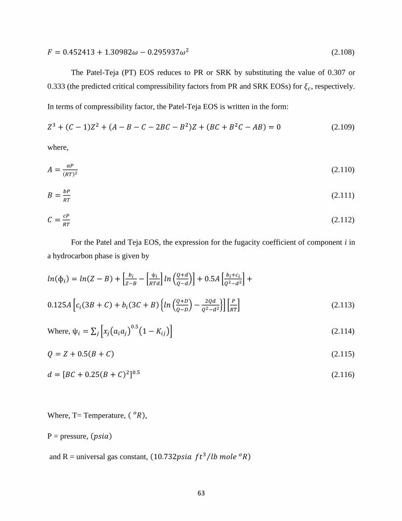
63
𝐹 = 0.452413 + 1.30982𝜔 − 0.295937𝜔2 (2.108)
The Patel-Teja (PT) EOS reduces to PR or SRK by substituting the value of 0.307 or
0.333 (the predicted critical compressibility factors from PR and SRK EOSs) for 𝜉𝑐, respectively.
In terms of compressibility factor, the Patel-Teja EOS is written in the form:
𝑍3 + (𝐶 − 1)𝑍2 + (𝐴 − 𝐵 − 𝐶 − 2𝐵𝐶 − 𝐵2)𝑍 + (𝐵𝐶 + 𝐵2𝐶 − 𝐴𝐵) = 0 (2.109)
where,
𝐴 =𝑎𝑃
(𝑅𝑇)2 (2.110)
𝐵 =𝑏𝑃
𝑅𝑇 (2.111)
𝐶 =𝑐𝑃
𝑅𝑇 (2.112)
For the Patel and Teja EOS, the expression for the fugacity coefficient of component i in
a hydrocarbon phase is given by
𝑙𝑛(ɸ𝑖) = 𝑙𝑛(𝑍 − 𝐵) + [𝑏𝑖
𝑍−𝐵− [
ѱ𝑖
𝑅𝑇𝑑] 𝑙𝑛 (
𝑄+𝑑
𝑄−𝑑)] + 0.5𝐴 [
𝑏𝑖+𝑐𝑖
𝑄2−𝑑2] +
0.125𝐴 [𝑐𝑖(3𝐵 + 𝐶) + 𝑏𝑖(3𝐶 + 𝐵) 𝑙𝑛 (𝑄+𝐷
𝑄−𝐷) −
2𝑄𝑑
𝑄2−𝑑2] [𝑃
𝑅𝑇] (2.113)
Where, ѱ𝑖 = ∑ [𝑥𝑗(𝑎𝑖𝑎𝑗)0.5
(1 − 𝐾𝑖𝑗)]𝑗 (2.114)
𝑄 = 𝑍 + 0.5(𝐵 + 𝐶) (2.115)
𝑑 = [𝐵𝐶 + 0.25(𝐵 + 𝐶)2]0.5 (2.116)
Where, T= Temperature, ( 𝑅𝑜 ),
P = pressure, (𝑝𝑠𝑖𝑎)
and R = universal gas constant, (10.732𝑝𝑠𝑖𝑎 𝑓𝑡3 𝑙𝑏 𝑚𝑜𝑙𝑒 𝑜𝑅⁄ )
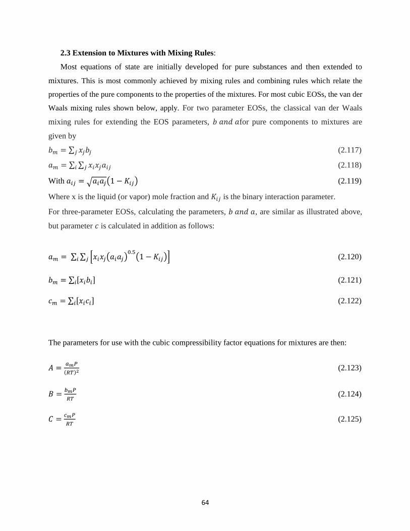
64
2.3 Extension to Mixtures with Mixing Rules:
Most equations of state are initially developed for pure substances and then extended to
mixtures. This is most commonly achieved by mixing rules and combining rules which relate the
properties of the pure components to the properties of the mixtures. For most cubic EOSs, the van der
Waals mixing rules shown below, apply. For two parameter EOSs, the classical van der Waals
mixing rules for extending the EOS parameters, 𝑏 𝑎𝑛𝑑 𝑎for pure components to mixtures are
given by
𝑏𝑚 = ∑ 𝑥𝑗𝑏𝑗𝑗 (2.117)
𝑎𝑚 = ∑ ∑ 𝑥𝑖𝑥𝑗𝑎𝑖𝑗𝑗𝑖 (2.118)
With 𝑎𝑖𝑗 = √𝑎𝑖𝑎𝑗(1 − 𝐾𝑖𝑗) (2.119)
Where x is the liquid (or vapor) mole fraction and 𝐾𝑖𝑗 is the binary interaction parameter.
For three-parameter EOSs, calculating the parameters, 𝑏 𝑎𝑛𝑑 𝑎, are similar as illustrated above,
but parameter 𝑐 is calculated in addition as follows:
𝑎𝑚 = ∑ ∑ [𝑥𝑖𝑥𝑗(𝑎𝑖𝑎𝑗)0.5
(1 − 𝐾𝑖𝑗)]𝑗𝑖 (2.120)
𝑏𝑚 = ∑ [𝑥𝑖𝑏𝑖]𝑖 (2.121)
𝑐𝑚 = ∑ [𝑥𝑖𝑐𝑖]𝑖 (2.122)
The parameters for use with the cubic compressibility factor equations for mixtures are then:
𝐴 =𝑎𝑚𝑃
(𝑅𝑇)2 (2.123)
𝐵 =𝑏𝑚𝑃
𝑅𝑇 (2.124)
𝐶 =𝑐𝑚𝑃
𝑅𝑇 (2.125)

65
2.4 Summary of Cubic Equations of State based on vdW’s Attractive Term Modification
Literature abounds with several cubic equations of state which have resulted from modifications
of the attraction term of vdW’s original equation of state. Table 2.1 shows the original form of
the vdW equation and other popular modifications of it. Also shown in Table 2.1 are the methods
of calculation of equation of state parameters ′𝑎 𝑎𝑛𝑑 𝑏′ for two-parameter EOSs and
′𝑎, 𝑏 𝑎𝑛𝑑 𝑐′ for three parameter EOSs.
TABLE 2.1: Structural Forms of Popular Cubic Equations of State and the EOS Parameters
REFERENCE EQUATION OF STATE
EOS Parameters
Van der Waal’s
(vdW),
1873
𝑃 =𝑅𝑇
𝑉 − 𝑏−
𝑎
𝑉2
𝑎 = (27𝑅2𝑇𝑐2) 64𝑃𝑐⁄ , 𝑏 = 𝑅𝑇𝑐 6𝑃𝑐⁄
Redlich-
Kwong
(RK),
1949
𝑃 =𝑅𝑇
𝑉 − 𝑏−
𝑎
𝑉(𝑉 + 𝑏)𝑇0.5
𝑎 = (0.4275𝑅2𝑇𝑐2.5) 𝑃𝑐⁄ , 𝑏 =
(0.08664𝑅𝑇𝑐) 𝑃𝑐⁄
Soave-Redlich-
Kwong
(SRK), 1972
𝑃 =𝑅𝑇
𝑉 − 𝑏−
𝑎𝑐𝛼(𝑇)
𝑉(𝑉 + 𝑏)
𝑎𝑐 = (0.42748𝑅2𝑇𝑐2) 𝑃𝑐⁄ , 𝑏 =
(0.08664𝑅𝑇𝑐) 𝑃𝑐⁄
Peng-Robinson
(PR),
1976
𝑃
=𝑅𝑇
𝑉 − 𝑏
−𝑎𝑐𝛼(𝑇)
𝑉(𝑉 + 𝑏) + 𝑏(𝑉 − 𝑏)
𝑎𝑐 = (0.45723𝑅2𝑇𝑐2) 𝑃𝑐⁄ , 𝑏 =
(0.07780𝑅𝑇𝑐) 𝑃𝑐⁄
Patel-Teja
(PT),
1982
𝑃
=𝑅𝑇
𝑉 − 𝑏
−𝑎𝑐𝛼(𝑇)
𝑉(𝑉 + 𝑏) + 𝑐(𝑉 − 𝑏)
𝑎𝑐 = Ω𝑎 𝑅2𝑇𝑐2 𝑃𝑐⁄ , 𝑏 = Ω𝑏 𝑅𝑇𝑐 𝑃𝑐⁄ and
𝑐 = Ω𝑐 𝑅𝑇𝑐 𝑃𝑐⁄ ,
Where Ω𝑏 is smallest root of the equation:
Ω𝑏3 + (2 − 3𝜉𝑐)Ω𝑏
2 + 3𝜉𝑐2Ω𝑏 − 𝜉𝑐
3 =0, Ω𝑐 = 1 − 3𝜉𝑐 and
Ω𝑎 = 3𝜉𝑐2 + 3(1 − 2𝜉𝑐)Ω𝑏 + Ω𝑏
2 +(1 − 3𝜉𝑐)
𝜉𝑐 = 0.329032 − 0.0767992𝜔+ 0.0211947𝜔2
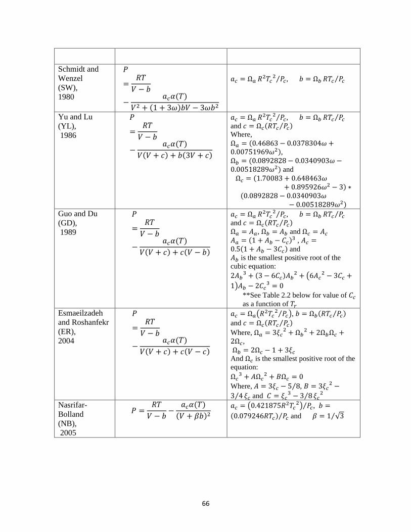
66
Schmidt and
Wenzel
(SW),
1980
𝑃
=𝑅𝑇
𝑉 − 𝑏
−𝑎𝑐𝛼(𝑇)
𝑉2 + (1 + 3𝜔)𝑏𝑉 − 3𝜔𝑏2
𝑎𝑐 = Ω𝑎 𝑅2𝑇𝑐2 𝑃𝑐⁄ , 𝑏 = Ω𝑏 𝑅𝑇𝑐 𝑃𝑐⁄
Yu and Lu
(YL),
1986
𝑃
=𝑅𝑇
𝑉 − 𝑏
−𝑎𝑐𝛼(𝑇)
𝑉(𝑉 + 𝑐) + 𝑏(3𝑉 + 𝑐)
𝑎𝑐 = Ω𝑎 𝑅2𝑇𝑐2 𝑃𝑐⁄ , 𝑏 = Ω𝑏 𝑅𝑇𝑐 𝑃𝑐⁄
and 𝑐 = Ω𝑐(𝑅𝑇𝑐 𝑃𝑐⁄ )
Where,
Ω𝑎 = (0.46863 − 0.0378304𝜔 +0.00751969𝜔2),
Ω𝑏 = (0.0892828 − 0.0340903𝜔 −0.00518289𝜔2) and
Ω𝑐 = (1.70083 + 0.648463𝜔+ 0.895926𝜔2 − 3) ∗
(0.0892828 − 0.0340903𝜔− 0.00518289𝜔2)
Guo and Du
(GD),
1989
𝑃
=𝑅𝑇
𝑉 − 𝑏
−𝑎𝑐𝛼(𝑇)
𝑉(𝑉 + 𝑐) + 𝑐(𝑉 − 𝑏)
𝑎𝑐 = Ω𝑎 𝑅2𝑇𝑐2 𝑃𝑐⁄ , 𝑏 = Ω𝑏 𝑅𝑇𝑐 𝑃𝑐⁄
and 𝑐 = Ω𝑐(𝑅𝑇𝑐 𝑃𝑐⁄ )
Ω𝑎 = 𝐴𝑎, Ω𝑏 = 𝐴𝑏 and Ω𝑐 = 𝐴𝑐
𝐴𝑎 = (1 + 𝐴𝑏 − 𝐶𝑐)3 , 𝐴𝑐 =0.5(1 + 𝐴𝑏 − 3𝐶𝑐) and
𝐴𝑏 is the smallest positive root of the
cubic equation:
2𝐴𝑏3 + (3 − 6𝐶𝑐)𝐴𝑏
2 + (6𝐴𝑐2 − 3𝐶𝑐 +
1)𝐴𝑏 − 2𝐶𝑐3 = 0
**See Table 2.2 below for value of 𝐶𝑐
as a function of 𝑇𝑟
Esmaeilzadeh
and Roshanfekr
(ER),
2004
𝑃
=𝑅𝑇
𝑉 − 𝑏
−𝑎𝑐𝛼(𝑇)
𝑉(𝑉 + 𝑐) + 𝑐(𝑉 − 𝑐)
𝑎𝑐 = Ω𝑎(𝑅2𝑇𝑐2 𝑃𝑐⁄ ), 𝑏 = Ω𝑏(𝑅𝑇𝑐 𝑃𝑐⁄ )
and 𝑐 = Ω𝑐(𝑅𝑇𝑐 𝑃𝑐⁄ )
Where, Ω𝑎 = 3𝜉𝑐2 + Ω𝑏
2 + 2Ω𝑏Ω𝑐 +2Ω𝑐,
Ω𝑏 = 2Ω𝑐 − 1 + 3𝜉𝑐
And Ω𝑐 is the smallest positive root of the
equation:
Ω𝑐3 + 𝐴Ω𝑐
2 + 𝐵Ω𝑐 = 0
Where, 𝐴 = 3𝜉𝑐 − 5 8⁄ , 𝐵 = 3𝜉𝑐2 −
3 4⁄ 𝜉𝑐 and 𝐶 = 𝜉𝑐3 − 3 8⁄ 𝜉𝑐
2
Nasrifar-
Bolland
(NB),
2005
𝑃 =𝑅𝑇
𝑉 − 𝑏−
𝑎𝑐𝛼(𝑇)
(𝑉 + 𝛽𝑏)2
𝑎𝑐 = (0.421875𝑅2𝑇𝑐2) 𝑃𝑐⁄ , 𝑏 =
(0.079246𝑅𝑇𝑐) 𝑃𝑐⁄ and 𝛽 = 1 √3⁄

67
TABLE 2.2: Value of 𝑪𝒄 as a Function of 𝑻𝒓
[See Guo and Du, 1989 EOS]
𝑻𝒓 𝑪𝒄
𝑇𝑟 < 0.8 0.308785
0.8 < 𝑇𝑟 < 1 0.308785 − 0.64(0.8 − 𝑇𝑟)2
1. 0 < 𝑇𝑟 < 1.2 0.308785 − 0.64(𝑇𝑟 − 1.2)2
𝑇𝑟 > 0.8 0.308785
2.5 Computation of Attraction Term Parameter for Cubic EOSs:
In most EOSs, the term ‘a’ is constant. With the exception of VDW, the term 𝑎𝛼(𝑇, 𝜔) is
temperature (T) and acentric (𝜔) factor dependent. A large variety of alpha functions have been
proposed through the years. Van der Waals (1873) originally took the alpha function, [𝛼(𝑇𝑟)] as
a constant. He realized later, and mentioned it in his Nobel lecture, that temperature dependence
was required in order to improve EOS performance. Soave (1972) is credited as being one of the
early successful contributors to this field. He showed that the alpha-function could be fitted to
vapor pressure data of each pure fluid. Soave’s alpha function is very popular with several EOS
and has the form:
𝛼(𝑇𝑟) = [1 + 𝑚(1 − 𝑇𝑟0.5)]
2 (2.126)
At the critical point, 𝑎𝛼(𝑇, 𝜔) = 1. (2.127)
Where, 𝑎𝑐 and 𝑚 are characteristic constants of substance.
Among EOSs that use the alpha function form proposed by Soave are Peng-Robinson’s (PR),
Soave-Redlich-Kwong’s (SRK), Pate-Teja’s (PT) and Schmidt-Wenzel’s (SW), to mention but
the popular ones. However, the slope 𝑚 has different values calculated for different equations of
state. A few, however, have different 𝛼-functions as seen in table 2.3 below:

68
TABLE 2.3: Selected Models for the Temperature Dependence of
the Attractive Term, 𝜶(𝑻𝒓) in CEOS
Equation of
State Expression for 𝜶(𝑻𝒓) 𝒎
Redlich and
Kwong
1 √𝑇𝑟⁄ Not applicable
Wilson (1964)
𝑇𝑟[1 + 𝑚(𝑇𝑟
−1 − 1)] 𝑚 = (1.57 + 1.62𝜔)
SRK 𝛼 = [1 + 𝑚(1 − 𝑇𝑟0.5)]
2 𝑚 = 0.48508 + 1.55171𝜔 − 0.15613𝜔2
PR 𝛼 = [1 + 𝑚(1 − 𝑇𝑟0.5)]
2 0.37464 + 1.54226𝜔𝑖 − 0.26992𝜔𝑖
2 , 𝑖𝑓 𝜔𝑖 ≤ 0.49
0.379642 + 1.48503𝜔𝑖 − 0.164423𝜔𝑖2 +
0.016666𝜔𝑖3 , 𝑖𝑓 𝜔𝑖 > 0.49
PT 𝛼 = [1 + 𝑚(1 − 𝑇𝑟0.5)]
2 𝑚 = 0.452413 + 1.30982𝜔 −
0.295937𝜔2
SW 𝛼 = [1 + 𝑚(1 − 𝑇𝑟0.5)]
2 For 𝜔 ≤ 0.4, 𝑚 = 𝑚1
For 𝜔 ≥ 0.55, 𝑚 = 𝑚2
0.4 < 𝜔 < 0.55, 𝑚 =[(𝜔 − 0.4) 0.15⁄ ]𝑚2 +[(0.55 − 𝜔) 0.15⁄ ]𝑚1 With
𝑚1 = 𝑚0 + (1 70⁄ )(5𝑇𝑟 − 3𝑚0 − 1)2,
𝑚2 = 𝑚0 + 0.71(𝑇𝑟 − 0.779)2,
𝑚0 = 0.465 + 1.347𝜔 − 0.528𝜔2, for
𝜔 ≤ 0.3671 and
𝑚0 = 0.5361 + 0.9593𝜔 for 𝜔 > 0.3671
GD 𝛼 = [1 + 𝑚(1 − 𝑇𝑟0.5)]
2 If 𝑇𝑟 ≤ 1.0, 𝑚 = 𝑚1(1.177631 −
0.553155𝑇𝑟 + 0.405622𝑇𝑟2)
where, 𝑚1 = 0.407290 + 1.461495𝜔 −0.233747𝜔2
If 𝑇𝑟 > 1.0, 𝑚 = 0.491987 + 1.285305𝜔 −0.685388𝜔2
69
2.6 Vapor-Liquid Equilibrium:
Thermodynamic equilibrium occurs when all net driving forces between a system and its
surroundings or between different parts of a system are zero, that is, all forces are in balance
across the system boundaries or between parts of the system, and there is no significant external
driving force. The difference between thermodynamic equilibrium and steady state systems is
that the net flow of matter or of energy is not just constant, as with steady state systems, but zero.
Macroscopic properties do not change with time nor with macroscopic position within a uniform
portion of the system which is at equilibrium state, O’Connell and Haile, 2005. Thus when a
system is in thermodynamic equilibrium, there will not be a spontaneous change in its
macroscopic properties. Disturbances of small interactions are often resisted by equilibrium state
systems which adjust to neutralize the interaction. This is called Le Chatelier’s principle, named
after Henry Loius Le Chatelier, who discovered it. A statement of the principle is, “When a
system at equilibrium is subjected to change in concentration, volume, temperature or pressure,
then the system readjusts itself to (partially) counteract the effect of the applied change and a
new equilibrium is established”.
Thermodynamic equilibrium encompasses thermal, mechanical, and chemical equilibrium.
Chemical equilibrium in turn, includes both diffusional and reaction equilibrium. For two phases,
say, 𝛼 𝑎𝑛𝑑 𝛽, in thermodynamic equilibrium, therefore, the following exist:
Thermal equilibrium: 𝑇𝛼 = 𝑇𝛽 (2.128)
Mechanical equilibrium: 𝑃𝛼 = 𝑃𝛽 (2.129)
Chemical equilibrium 𝜇𝑖𝛼 = 𝜇𝑖
𝛽 (2.130)
or diffusional equilibrium 𝑓𝑖𝛼 = 𝑓𝑖
𝛽 (2.131)
Equation (2.131) is a consequence of Eq. (2.130). Since fugacity is a measure of the potential for
transfer of a component between two phases, equal fugacities of a component in both phases
results in zero net transfer.

70
In thermodynamic equilibrium, all kinds of equilibrium hold at once and indefinitely, until
disturbed by a thermodynamic operation. Gas and liquid co-existence is common to several
petroleum and natural gas applications, particularly, in the reservoir, pipeline, separators, oil and
LNG tankers, storage tanks, wellbore, LNG and NGL processing. Vapor-liquid equilibria
problems in the industry include determination of phase boundaries which involves calculations
of bubble point and dew point temperatures and pressures, and flash calculations which involve
relative phase quantity and quality determinations. Phase quantity determination entails
calculation of molar fractions of gas and liquid phases while the phase quality determination
involves determination of gas and liquid phase compositions at equilibrium.
Flash calculations can be simplified by considering for example, that “𝐹” moles of feed with
a composition, 𝑧𝑖, having 𝑛𝑐 number of components enter an equilibrium cell at a given
temperature and pressure, figure 2.3. Flash vaporization occurs resulting in ‘𝑉’ moles of vapor
of composition, ‘𝑦𝑖’ and ‘𝐿’ moles of liquid of composition, ‘𝑥𝑖’.
Figure 2.4: Flash Vaporization at a given Temperature and Pressure
Assuming steady state, an overall balance is taken as:
𝐹 = 𝑉 + 𝐿 (2.132)
𝐶𝑜𝑚𝑝𝑜𝑠𝑖𝑡𝑖𝑜𝑛 = 𝑧𝑖
𝑖 = 1,2, . . . , 𝑛𝑐
F Moles, Feed
𝐶𝑜𝑚𝑝𝑜𝑠𝑖𝑡𝑖𝑜𝑛 = 𝑦𝑖
V moles, vapor
𝐶𝑜𝑚𝑝𝑜𝑠𝑖𝑡𝑖𝑜𝑛 = 𝑥𝑖
L moles, liquid
𝛼𝑔 =𝑉
𝐹
𝛼𝑙 =𝐿
𝐹
71
Defining the fractions of gas as:
𝛼𝑔 =𝑉
𝐹 (2.133)
and the fraction of liquid as:
𝛼𝑙 =𝐿
𝐹 (2.134)
so that, 𝛼𝑔 + 𝛼𝑙 = 1 (2.135)
The steady state assumption and conservation of every component in the system gives:
𝑦𝑖𝛼𝑔 + 𝑥𝑖𝛼𝑙 = 𝑧𝑖 (2.136)
where, 𝑖 = 1,2, . . . , 𝑛𝑐 (2.137)
This can be re-written as:
𝑦𝑖𝛼𝑔 + 𝑥𝑖(1 − 𝛼𝑔) = 𝑧𝑖 (2.138)
And noting that equilibrium constant is defined as:
𝐾𝑖 =𝑦𝑖
𝑥𝑖, (2.139)
Equation (2.138) is written in terms of eq. (2.139) as:
𝑦𝑖𝛼𝑔 +𝑦𝑖
𝐾𝑖(1 − 𝛼𝑔) = 𝑧𝑖 (2.140)
Solving for 𝑦𝑖, gives the vapor phase composition:
𝑦𝑖 =𝑧𝑖𝐾𝑖
1+𝛼𝑔(𝐾𝑖−1) (2.141)
It can be shown that, the liquid phase composition is:
𝑥𝑖 =𝑧𝑖
1+𝛼𝑔(𝐾𝑖−1) (2.142)
Given the constraint that all molar fractions must sum to unity, i.e.

72
∑ 𝑦𝑖 = 1𝑛𝑐𝑖=1 , (2.143)
this can be substituted into above equation to give the objective function:
∑𝑧𝑖𝐾𝑖
1+𝛼𝑔(𝐾𝑖−1)= 1
𝑛𝑐𝑖=1 (2.144)
So that 𝐹𝑦(𝛼𝑔) = ∑𝑧𝑖𝐾𝑖
1+𝛼𝑔(𝐾𝑖−1)− 1 = 0
𝑛𝑐𝑖=1 (2.145)
And 𝐹𝑥(𝛼𝑔) = ∑𝑧𝑖
1+𝛼𝑔(𝐾𝑖−1)− 1 = 0
𝑛𝑐𝑖=1 (2.146)
By letting 𝐹(𝛼𝑔) = 𝐹𝑦(𝛼𝑔) − 𝐹𝑥(𝛼𝑔), (2.147)
a new objective function is obtained as
𝐹(𝛼𝑔) = ∑𝑧𝑖(𝐾𝑖−1)
1+𝛼𝑔(𝐾𝑖−1)− 1 = 0
𝑛𝑐𝑖=1 (2.148)
This new objective function is known in literature as the Rachford-Rice objective
function, named after the authors, Rachford, H. H. and Rice, J. D. who first derived it in 1952. It
is a non-linear equation in one variable and is solved using the Newton-Raphson iterative
technique. The method, which has a fast convergence rate, calculates a new estimate, 𝛼𝑔𝑛𝑒𝑤,
which is closer to the answer than the initial guess, or previous value, 𝛼𝑔𝑜𝑙𝑑 as follows:
𝛼𝑔𝑛𝑒𝑤 = 𝛼𝑔
𝑜𝑙𝑑 −𝐹(𝛼𝑔
𝑜𝑙𝑑)
𝐹′(𝛼𝑔𝑜𝑙𝑑)
(2.149)
Where 𝐹′(𝛼𝑔𝑜𝑙𝑑) is the first derivative of the Rachford-Rice objective function and has the
value:
∑𝑧𝑖(𝐾𝑖−1)2
[1+𝛼𝑔(𝐾𝑖−1)]2 − 1 = 0𝑛𝑐𝑖=1 . (2.150)
Equation (2.149) is therefore written out as:
𝛼𝑔𝑛𝑒𝑤 = 𝛼𝑔
𝑜𝑙𝑑 +∑
𝑧𝑖(𝐾𝑖−1)
1+𝛼𝑔(𝐾𝑖−1)
𝑛𝑐𝑖=1
∑𝑧𝑖(𝐾𝑖−1)2
[1+𝛼𝑔(𝐾𝑖−1)]2𝑛𝑐𝑖=1
(2.151)

73
𝐾𝑖′𝑠 are calculated using Wilson’s empirical correlation:
𝐾𝑖 =1
𝑃𝑟𝑖
𝐸𝑋𝑃 [5.37(1 + 𝜔𝑖) (1 −1
𝑇𝑟𝑖
)] (2.152)
Usually, convergence is achieved when the absolute value of
|𝛼𝑔𝑛𝑒𝑤 − 𝛼𝑔
𝑜𝑙𝑑| = 휀 (2.153)
Where, 휀 is a small number (휀 = 1.0 ∗ 10−9 is usually adequate).
Once the fraction of gas in the mixture, 𝛼𝑔, has been obtained, the fraction of liquid is calculated
from
𝛼𝑙 = 1 − 𝛼𝑔 (2.154)
2.6.1 Equilibrium Constant
Equilibrium constants are defined as the ratio of mole fractions of components in the vapor
phase to the mole fraction of the same components in the liquid phase, (Eq.(2.139)). The
equilibrium ratios or 𝐾𝑖 values are required to solve the Rachford-rice objective function. A first
approximation of these values is obtained from Wilson’s correlation, Eq. (2.152). However,
Wilson’s correlation yields only approximate values for equilibrium ratios. More reliable
predictions of 𝐾𝑖 values is obtained by applying the thermodynamic equilibrium considerations
of chemical potential equality, and updating values of 𝐾𝑖 by the so-called Successive Substitution
Method.
Recall Eq. (2.131): 𝑓𝑖𝛼 = 𝑓𝑖
𝛽
For a vapor-liquid equilibrium as with hydrocarbons, the equality of fugacity equation is more
specifically expressed as:
𝑓𝑖𝑔 = 𝑓𝑖
𝑙 (2.155)
74
Where, 𝑓𝑖𝑔
is the fugacity of the i-th component in the gas phase and 𝑓𝑖𝑙 is the fugacity of the i-th
component in the liquid phase. The fugacity coefficient is defined as the ratio of the fugacity of
substance to its partial pressure. For a vapor-liquid system consisting of 𝑛𝑐 components, the
fugacity coefficients of component 𝑖 in the vapor and liquid phases, respectively, is written as:
∅𝑖𝑔 =
𝑓𝑖𝑔
𝑦𝑖𝑃 (2.156)
∅𝑖𝑙 =
𝑓𝑖𝑙
𝑥𝑖𝑃 (2.157)
𝑖 = 1, 2, 3, … , 𝑛𝑐
It can be shown that equilibrium constants are related to fugacity coefficients as follows:
𝐾𝑖 =∅𝑖
𝑙
∅𝑖𝑔 =
𝑓𝑖𝑙 𝑥𝑖𝑃⁄
𝑓𝑖𝑔 𝑦𝑖𝑃⁄
=𝑦𝑖
𝑥𝑖(
𝑓𝑖𝑙
𝑓𝑖𝑔) (2.158)
For the representation of van-der Waals type equations of state in the generalized form
as:
22 wuvv
Ta
bV
RTP
(2.159)
The fugacity coefficient of component 𝑖 in the vapor and liquid phases can be calculated from
the generalized forms:
𝑙𝑛∅𝑖𝑙 = (𝑍𝑙 − 1) − 𝑙𝑛(𝑍𝑙 − 𝐵) +
𝐴
√𝑈2+4𝑊2𝑙𝑛
2𝑍𝑙+𝑈−√𝑈2+4𝑊2
2𝑍𝑙+𝑈+√𝑈2+4𝑊2 (2.160)
𝑙𝑛∅𝑖𝑔 = (𝑍𝑔 − 1) − 𝑙𝑛(𝑍𝑔 − 𝐵) +
𝐴
√𝑈2+4𝑊2𝑙𝑛
2𝑍𝑔+𝑈−√𝑈2+4𝑊2
2𝑍𝑔+𝑈+√𝑈2+4𝑊2 (2.161)
The compositions of the vapor and liquid phases calculated by Eqs. (2.141) and (2.142),
respectively, are used for calculating compressibility factors for vapor (𝑍𝑔) and liquid (𝑍𝑙) phases
to be used in Eqs. (2.160) and (2.161) above.

75
2.6.1(a) Successive Substitution Method (SSM)
The starting point is by use of the Wilson’s correlation to calculate initial 𝐾𝑖′𝑠. This is
used with the Rachford-Rice equation to obtain fraction of gas, 𝛼𝑔, 𝑎𝑛𝑑 𝑡ℎ𝑢𝑠, 𝑦𝑖 𝑎𝑛𝑑 𝑥𝑖 . Using,
𝑦𝑖 𝑎𝑛𝑑 𝑥𝑖, values of 𝑍𝑔 𝑎𝑛𝑑 𝑍𝑙, respectively are calculated. Then, using Eqs. (2.160) and (2.161),
the fugacity coefficients for both phases are calculated. Fugacities of liquid and vapor phases are,
respectively calculated from the fugacity coefficients as:
𝑓𝑖𝑙 = ∅𝑖
𝑙 ∗ 𝑥𝑖𝑃 (2.162)
And
𝑓𝑖𝑔 = ∅𝑖
𝑔 ∗ 𝑦𝑖𝑃 (2.163)
Convergence is achieved when
∑ (𝑓𝑖
𝑙
𝑓𝑖𝑔 − 1)
2
< 10−14𝑛𝑐𝑖=1 (2.164)
At convergence, the resulting 𝐾𝑖 values are the final accurate equilibrium ratios. If the
convergence criterion is not met, the 𝐾𝑖 values are updated. The correction step to find 𝐾𝑖 in
SSM is written as:
𝐾𝑖𝑛+1 = (
𝑦𝑖
𝑥𝑖)
𝑛
(𝑓𝑖
𝑙
𝑓𝑖𝑔)
𝑛
𝐾𝑖𝑛+1 = 𝐾𝑖
𝑛 (𝑓𝑖
𝑙
𝑓𝑖𝑔)
𝑛
(2.165)

76
2.6.1(b) Accelerated Successive Substitution Method (ASSM)
Fugacities are strongly dependent on the compositions at conditions close to the critical
which often results in a slowing down of convergence. Rinses et al. (1981) presented a method
which would overcome the slow convergence problem. This method, called the accelerated
successive Substitution Method (ASSM) has the following steps:
1. The SSM technique is used to initiate the updating of the Ki-values the first time.
2. All of the following criteria are checked at every step during iterations using the SSM:
(i) ∑ (𝑅𝑟𝑖
𝑛𝑒𝑤−1)2𝑛𝑐
𝑖=1
∑ (𝑅𝑟𝑖𝑜𝑙𝑑−1)
2𝑛𝑐𝑖=1
≥ 0.8 (2.166)
(ii) |𝛼𝑔𝑛𝑒𝑤 − 𝛼𝑔
𝑜𝑙𝑑| ≤ 0.1 (2.167)
(iii) 10−5 ≤ ∑ (𝑅𝑟𝑖
𝑛𝑒𝑤 − 1)2
≤ 10−3𝑛𝑐𝑖=1 (2.168)
(iv) 0 ≤ 𝛼𝑔𝑛𝑒𝑤 ≤ 1 (2.169)
These criteria assure that sufficient proximity to the conditions which ensure efficiency of
the method exsist. 𝑅𝑟𝑖 is the ratio of liquid fugacity to gas fugacity of the i-th component:
i.e. 𝑅𝑟𝑖=
𝑓𝑖𝑙
𝑓𝑖𝑣 (2.170)
and ‘𝛼𝑔’ is molar gas fraction of the two-phase system.
If the system satisfies ALL the above criteria, the iteration technique is then switched
from the SSM to the ASSM. Otherwise, SSM is used for the update of the Ki-values The
ASSM technique for updating 𝐾𝑖 is
𝐾𝑖𝑛𝑒𝑤 = 𝐾𝑖
𝑜𝑙𝑑𝑅𝑟𝑖
𝜆𝑖
(2.171)
Where, 𝜆𝑖 = [(𝑅𝑟𝑖
𝑜𝑙𝑑−1)
(𝑅𝑟𝑖𝑜𝑙𝑑−𝑅𝑟𝑖
𝑛𝑒𝑤)] (2.172)
3. In some cases, using a constant acceleration value of 𝜆𝑖 = 2 is good enough.

77
4. Once all the criteria in step (2) are satisfied, skip step (2) for the subsequent iterations and
use the ASSM technique to update Ki-values until convergence is attained, unless it does
not give acceptable new estimates (as stated next).
5. When ASSM is used, it must always be tested to show that it leads to an improved
solution (i.e., that it brings fugacity ratios closer to unity). If not, it must be rejected and
switched back to SSM.
Fugacity ratios are checked to be sure that they approach unity; otherwise SSM is preferred in
place of ASSM. (Mehra et. al (1983)).

78
CHAPTER THREE
3.0 METHODOLOGY
The new equation was developed by semi-empirical methods. These are methods based
partly on analytical and partly empirical (that is, derived from experimental data) derivations.
3.1 Development and Formulation Considerations for New EOS
Certain research on EOS formulations have suggested that the van der Waal-type equations
of state are more accurate in the attractive term than in the repulsive term (Jacobson et al., 2000)
and that accurate repulsive terms are crucial in equations of state since repulsive molecular
forces are dominant at high densities. This suggestion is partly responsible for the modifications
based on the repulsive term. Modifications based on the attraction term are also popular amongst
researchers based on the simplicity of resulting EOS and established ease of solution by
analytical techniques. In most cases, new equations were formed by matching volumetric or
vapor-pressure parameters to experimentally measured data (i.e. by empirical means). In recent
times, major formulation considerations are dependent on the findings of Adachi et al., 1983 and
Zhi, et. Al., 2000:
(i) The representation of the liquid compressibility factor is mainly controlled by the
repulsive term.
(ii) Rigorous or complex repulsive terms provide no real advantage over the van der
Waals type repulsive term, which was considered the most suitable one.
(iii) The attraction is a function of temperature (previously known) and volume.
(previously unknown or un-asserted)
(iv) Improvements in the attractive term are influenced by the number of terms present
when the EOS is expressed in terms of a 𝜋(𝑉) function and the relationship between
the numerators of the various terms.
The 𝜋(𝑉) function is derived by first noting that all vdW type EOSs can be represented in the
form:
𝑃 =𝑅𝑇
𝑉−𝑏−
𝑎𝑤
𝜋(𝑉)𝑉2 (3.1)
79
Where b and a, are constants with their usual meanings and subscript 𝑤 means ‘associated with
the vdW EOS.’
This was derived by noting that the van der Waals EOS can be written in the form:
𝑃 =𝑅𝑇
𝑉−𝑏−
𝑎𝑤
𝑉2 (3.2)
The first improvement over the vdW’s EOS to be reckoned with was by Redlich and
kwong (1949) which though written as:
𝑃 =𝑅𝑇
𝑉−𝑏−
𝑎(√𝑇)−1
𝑉(𝑉+𝑏) (3.3)
can be expressed in 𝜋(𝑉) function as:
𝑃 =𝑅𝑇
𝑉−𝑏−
𝑎𝑅𝐾𝑆
𝑉(𝑉+𝑏) (3.4)
Where 𝑎𝑅𝐾𝑆 is dependent on temperature.
Assuming that 𝑎𝑤 is not a constant, and making Eq.(3.4) equal to Eq.(3.2), i.e.
𝑎𝑤
𝑉2 =𝑎𝑅𝐾𝑆
𝑉(𝑉+𝑏) (3.5)
Then, after rearranging, the 𝑎𝑤 can be calculated as
𝑎𝑤 =𝑎𝑅𝐾𝑆
1+𝑏 𝑉⁄=
𝑎𝑅𝐾𝑆
𝜋𝑅𝐾𝑆(𝑉) (3.6)
Where 𝜋(𝑉) is a new function which expresses the influence of volume on the attractive
parameter, 𝑎𝑤.
In like manner, for the Peng Robinson’s (PR) EOS (1976)
𝑃 =𝑅𝑇
𝑉−𝑏−
𝑎𝑃𝑅
𝑉(𝑉+𝑏)+𝑏(𝑉−𝑏) (3.7)
With the 𝑎𝑤 expressed similarly as:
𝑎𝑤 =𝑎𝑃𝑅
1+(2𝑏 𝑉)⁄ −(𝑏2 𝑉2)⁄=
𝑎𝑃𝑅
𝜋𝑃𝑅(𝑉) (3.8)
80
Similarly, for Martin’s EOS (1979), which has the form,
𝑃 =𝑅𝑇
𝑉−𝑏−
𝑎𝑀
(𝑉+𝑐)2 (3.9)
𝑎𝑤 =𝑎𝑀
1+(2𝑐 𝑉)+(𝑐2 𝑉2)⁄⁄=
𝑎𝑀
𝜋𝑀(𝑉) (3.10)
Also, for the Patel Teja (PT) (1982) EOS:
𝑃 =𝑅𝑇
𝑉−𝑏−
𝑎𝑃𝑇
𝑉(𝑉+𝑏)+𝑐(𝑉−𝑏) (3.11)
𝑎𝑤 =𝑎𝑃𝑇
1+((𝑏+𝑐) 𝑉)−(𝑐𝑏 𝑉2)⁄⁄=
𝑎𝑃𝑇
𝜋𝑃𝑇(𝑉) (3.12)
For the Adachi-Lu-Sugie (ALS) EOS (1983)
𝑃 =𝑅𝑇
𝑉−𝑏1−
𝑎𝐴𝐿𝑆
(𝑉−𝑏2)(𝑉+𝑏3) (3.13)
𝑎𝑤 =𝑎𝐴𝐿𝑆
1+((𝑏3−𝑏2) 𝑉)−(𝑏2𝑏3 𝑉2)⁄⁄=
𝑎𝐴𝐿𝑆
𝜋𝐴𝐿𝑆(𝑉) (3.14)
The major conclusions drawn by the authors from these expressions are:
First, that the form of the 𝜋(𝑉) function for the various vdW type EOS’s account for the
differences in their predictive capabilities. An improvement in the attractive term is influenced
by the number of terms present when the EOS is expressed in terms of a 𝜋(𝑉) function. The
𝜋(𝑉) function which in general, has the form:
𝜋(𝑉) = 1 +𝑘
𝑉+
𝑙
𝑉2+ ⋯ (3.15)
is a major determinant of EOS accuracy. The more the numbers of terms present in the 𝜋(𝑉)
function, the better the accuracy of the corresponding EOS.
For example, the forms of 𝑎(𝑇) in PR and RKS EOSs are the same:
𝑎 = 𝑎𝑐𝛼(𝑇𝑟) (3.16)
𝛼(𝑇𝑟)0.5 = 1 + 𝑚(1 − 𝑇𝑟0.5) (3.17)

81
where, 𝑎𝑐 and 𝑚 are characteristic constants of substances. In spite of this seeming similarity, the
PR EOS gives better accuracy than the RKS EOS in liquid volume and density predictions. This
is due mainly to the form of the 𝜋(𝑉) functions, which for PR is:
𝜋𝑃𝑅(𝑉) = 1 +2𝑏
𝑉−
𝑏2
𝑉2 (3.18)
This is superior in terms of expressing the influence of volume based on the number of terms
involving volume in the denominator, which is more in comparison to the 𝜋(𝑉) of the RKS
which is:
𝜋𝑅𝐾𝑆(𝑉) = 1 +𝑏
𝑉 (3.19)
The 𝜋𝑅𝐾𝑆(𝑉) has only two terms only one of which has a v dependence, which gives it less
competition in terms of accuracy when compared to other vdW type EOSs with more (e.g. three)
terms.
The form of the 𝜋(𝑉) function for the martin EOS is similar to that of the PR EOS, so
both have almost identical degrees of accuracy. In similar reasoning, the PT EOS and the ALS
EOS are better than the accuracies of the RKS and PR EOSs because of their 𝜋(𝑉) functions
given as:
𝜋𝑃𝑇(𝑉) = 1 +(𝑏+𝑐)
𝑉−
𝑐𝑏
𝑉2 (3.20)
𝜋𝐴𝐿𝑆(𝑉) = 1 +(𝑏3−𝑏2)
𝑉−
𝑏2𝑏3
𝑉2 (3.21)
When compared to the 𝜋(𝑉) forms of the RKS and PR (Eq. 3.19 and 3.18), the PT and
ALS EOS, Eq. (3.20) and Eq. (3.21) are more elastic, powerful and so more competent for the
regression of data. They therefore give better accuracy when compared to the accuracies of the
PR and RKS EOSs.
Also, the relations between the parameter 𝑘, 𝑙, … in Eq.(3.15) also influence the capability
of an EOS in predicting vapor-liquid thermodynamic properties. The stronger the relation
between 𝑘 𝑎𝑛𝑑 𝑙, the poorer the predictive ability of the EOS and vice versa. For example, the
82
relation between the parameters 𝑘 𝑎𝑛𝑑 𝑙 in 𝜋𝑃𝑅(𝑉) and 𝜋𝑀(𝑉) are very strong which therefore,
limit the capabilities of PR and Martin EOSs, while the parameters 𝑘 𝑎𝑛𝑑 𝑙 in 𝜋𝑃𝑇(𝑉) and
𝜋𝐴𝐿𝑆(𝑉) are relatively weak, guaranteeing better performance for these than the PR, Martin, RKS
and other EOSs for the calculation of various properties of fluids.(Baker and Diamond, 2000)
Finally, the author predicted that by improving 𝜋(𝑉) function, it would be possible to
develop a better vdW type EOS. Building on this theory, a structural form which builds upon the
strength of the PT EOS and stretches it’s 𝜋(𝑉) 𝑓𝑢𝑛𝑐𝑡𝑖𝑜𝑛 is proposed. The resulting form is
made to improve upon the prediction performance guaranteed by the PT EOS by ensuring that
the additional parameter is more dependent on the critical compressibility factor term reflected
by the ‘c’ term.
3.2 Reasons for Choice of Cubic EOS
The following are some reasons why the new equation proposed is based on the van der
Waal type cubic equations of state model.
i. Cubic equations of state are popular in the petroleum industry for modeling phase
equilibria and thermodynamic properties of hydrocarbon mixtures for decades now
because of their simplicity and reasonable degree of accuracy.
ii. Several well studied and understood analytical algorithms abound in the field of
Mathematics and Engineering which can be applied to solve the resulting cubic in
volume or compressibility factor equations
iii. Cubic equations of state present correct limiting behavior such that, as 𝑃 → ∞, 𝑉 →
𝑏, where 𝑏 is co-volume or molecular volume.
iv. Whilst cubic equations are derived, first for pure components, their extension to
mixtures is relatively easy by use of mixing rules which result in reasonable
accuracies.
v. For most applications cubic EOSs can be tuned to improve the accuracy in estimation
of volumetric or thermodynamic properties.

83
3.3 Derivation of New Cubic EOS
Yun et al. (2000), in their conclusion, noted that improved performance may be
guaranteed by improving either the number of terms on the 𝜋(𝑉) function or minimizing the
strength of the interaction between the numerator terms, i. e. the k, l, m, etc. terms. The former if
implemented beyond a power of two, would result in a higher than three order of polynomial,
which is not simple. Therefore, the one choice left is to reduce the strength of either the k or l
terms. Essentially, the alternative resulting forms must further satisfy the condition that it results
in unbiased results of measured properties, by minimizing the error in the prediction of vapor
pressure and liquid density data when referenced to 172 experimental data values (obtained from
literature) for various pure components over a wide range of temperature and pressure. The
starting model was intuitively reasoned to be one that would give prominence to the critical point
effects, captured by the critical compressibility factor parameter, 𝑐, shown to be the source of
weakness of several other existing EOSs.
About 153 structural forms which satisfy these conditions were developed and each one
tested with empirical data to ascertain their performance. The only form which minimized error
considerably, between predicted and experimentally determined values has a final form shown
below as Eq. (3.22). The resultant form which gave optimal error minimization in measurement
of both fluid compressibility factors and liquid densities has the structural form:
𝑃 =𝑅𝑇
𝑉−𝑏−
𝑎𝑐𝛼(𝑇)
𝑉(𝑉+𝑏)+𝑐(𝑉−𝑏)+𝑐(𝑐−𝑏) (3.22)
The New EOS, Eq.(3.22) has a 𝜋(𝑉) function which not only satisfies the Yun et
al.(2000) suggested requirements for improved performance when compared to the PT EOS but
actually does. The 𝜋(𝑉) function is:
𝜋𝑁𝐸𝑊(𝑉) = 1 +(𝑏+𝑐)
𝑉−
(2𝑏𝑐−𝑐2)
𝑉2 (3.23)
The NEW EOS expressed in terms of compressibility factor is:
𝑍3 + (𝐶 − 1)𝑍2 + (𝐴 − 𝐵 − 𝐶 − 3𝐵𝐶 − 𝐵2 + 𝐶2)𝑍 + (2𝐵𝐶 + 2𝐵2𝐶 − 𝐵𝐶2 − 𝐶2 − 𝐴𝐵) = 0 (3.24)
Where, the terms 𝐴, 𝐵 𝑎𝑛𝑑 𝐶 have the usual meanings as in other three-parameter EOS such as PT EOS,
for example.
84
𝐴 =𝑎𝑃
(𝑅𝑇)2 (3.25)
𝐵 =𝑏𝑃
𝑅𝑇 (3.26)
𝐶 =𝑐𝑃
𝑅𝑇 (3.27)
3.4 Determination of m-Parameter in Alpha-Function [𝜶(𝑻𝒓)] for New EOS
The eventual value of 𝑚, which is unique for most structural forms, is a very relevant parameter
for EOS tuning to achieve enhanced performance. The alpha function of Soave, (Eq. 2.137),
which is adopted for several modern equations of state is also used for the new equation of state.
However, the m-parameter, which is critical in tuning EOSs to improve accuracy in
thermodynamic properties’ estimation, was derived statistically. The form of the m-parameter is
such that it corresponds to format which are determined statistically using regression methods.
There are several modern regression methods, such as Additive and Variance Stabilizing
Transformation (AVAS), Alternating Conditional Expectations (ACE), Least Trimmed Squares
Regression (LTSREG), Progression Pursuit Regression (PPREG) and Fit Linear Regression
(FLR).
3.4.1 Alternating Conditional Expectation (ACE)
The alternating conditional expectation (ACE) algorithm of Breiman and Friedman
(1985) was used because, in regression analysis, where the effect of one or more independent
variables (predictors or covariates) on a dependent variable (response) is sought, use of ACE has
shown tremendous ability to identify the correct functional forms, reveal more accurate
relationships, and to considerably improve the model fit. The algorithm for the ACE is also easy
to comprehend.
The general form of a multiple linear regression model for 𝑁 independent variables
(predictors), say𝑋1, 𝑋2,...,𝑋𝑁 , and a response variable 𝑌 is given by:
𝑌 = 𝛽0 + ∑ 𝛽𝑖𝑋𝑖 + 𝜖𝑁𝑖=1 (3.28)

85
Where, 𝛽0, 𝛽1, 𝛽2, ….𝛽𝑁 are the regression coefficients to be estimated, and 𝜖 is an error term.
The above equation suggests that the response variable, 𝑌 is a combination of linear effects of
𝑋1, 𝑋2,..., 𝑋𝑁 and a random error component 𝜖.
Conditions are that the expectation,
𝐸[∈] = 0, (3.29)
𝑉𝑎𝑟[∈] = 𝜎2 (3.30)
and 𝜖 is independent of 𝑥1, 𝑥2, … , 𝑥𝑛. (3.31)
The simplest Additive Model (AM) has the form:
𝐸[𝑌𝑖] = 𝛽0 + ∑ 𝑓𝑗(𝑥𝑖𝑗)𝑁𝑗=1 (3.32)
Where the 𝑓𝑖′𝑠 are unknown smooth functions fit from the data of interest. Since the fj are
estimated from the data, one avoids the traditional assumption of linearity in the
explanatory variables; however, AM retains the assumption that explanatory variable
effects are additive. Therefore, the response is modeled as the sum of arbitrary smooth
univariate functions of the explanatory variables, but not as the sum of multivariate
functions of the explanatory variables.
One needs a reasonably large sample size to estimate each fj , though the sample
size requirement grows only linearly in the number 𝑁.
The basic assumptions are as before except that in addition, 𝐸[𝑓𝑗(𝑥𝑖𝑗)] = 0 in order to
prevent identifiability problems. The parameters in the additive model are
𝑓𝑗, 𝛽0 𝑎𝑛𝑑 𝜎2.
The alternating conditional expectations (ACE) algorithm, developed by Breiman and
Friedman (1985), fits the model
𝐸[𝑔(𝑌𝑖)] = 𝛽0 + ∑ 𝑓𝑗(𝑋𝑖𝑗)𝑁𝑗=1 (3.33)
Where, all conditions are as given for the AM, except g is an unspecified function, scaled
to satisfy the technically necessary constraint that var[g(Y )] = 1 (otherwise, the zero
transformation would be trivially perfect).
Given variables 𝑌𝑖 and 𝑿𝒊, one wants 𝑔 and 𝑓1, … . 𝑓𝑁 such that
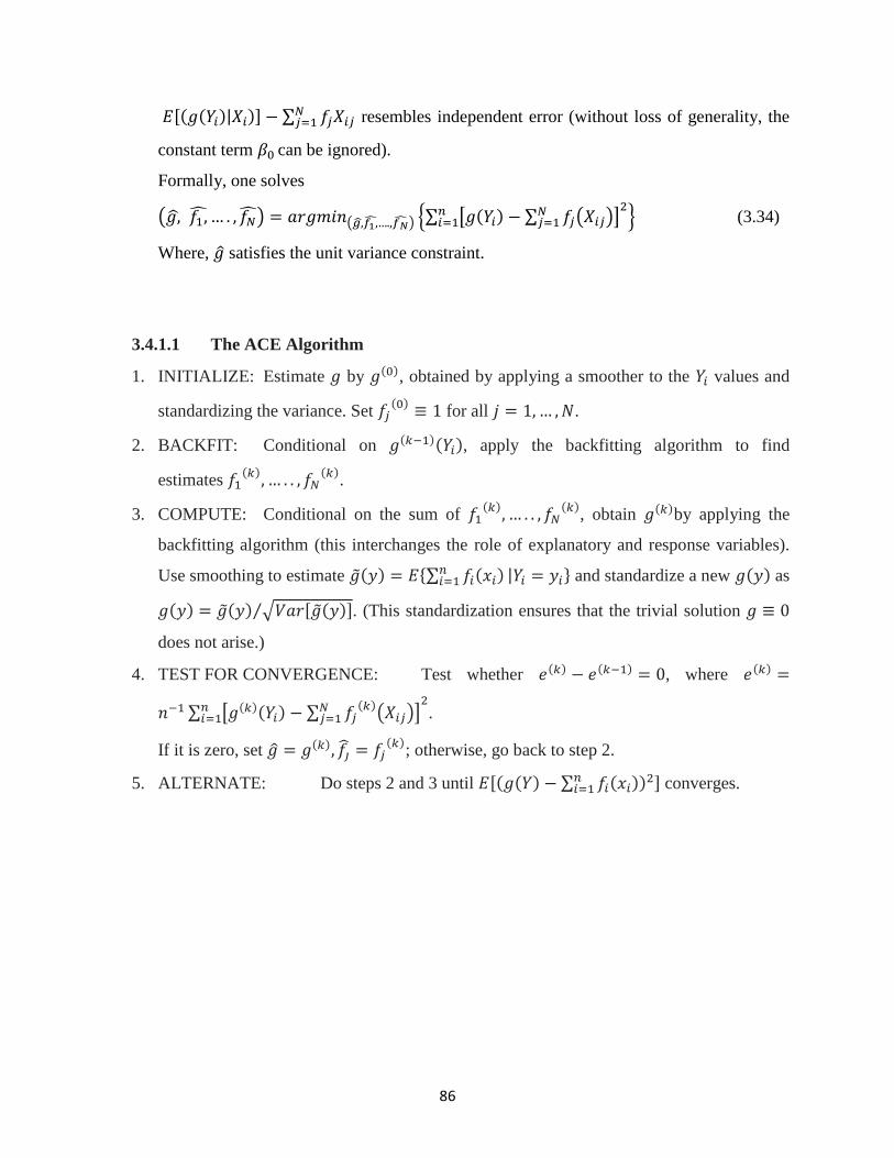
86
𝐸[(𝑔(𝑌𝑖)|𝑋𝑖)] − ∑ 𝑓𝑗𝑋𝑖𝑗𝑁𝑗=1 resembles independent error (without loss of generality, the
constant term 𝛽0 can be ignored).
Formally, one solves
(𝑔, 𝑓1 , … . , 𝑓) = 𝑎𝑟𝑔𝑚𝑖𝑛(𝑔,𝑓1 ,….,𝑓) ∑ [𝑔(𝑌𝑖) − ∑ 𝑓𝑗(𝑋𝑖𝑗)𝑁𝑗=1 ]
2𝑛𝑖=1 (3.34)
Where, satisfies the unit variance constraint.
3.4.1.1 The ACE Algorithm
1. INITIALIZE: Estimate 𝑔 by 𝑔(0), obtained by applying a smoother to the 𝑌𝑖 values and
standardizing the variance. Set 𝑓𝑗(0)
≡ 1 for all 𝑗 = 1, … , 𝑁.
2. BACKFIT: Conditional on 𝑔(𝑘−1)(𝑌𝑖), apply the backfitting algorithm to find
estimates 𝑓1(𝑘)
, … . . , 𝑓𝑁(𝑘)
.
3. COMPUTE: Conditional on the sum of 𝑓1(𝑘)
, … . . , 𝑓𝑁(𝑘)
, obtain 𝑔(𝑘)by applying the
backfitting algorithm (this interchanges the role of explanatory and response variables).
Use smoothing to estimate (𝑦) = 𝐸∑ 𝑓𝑖(𝑥𝑖)𝑛𝑖=1 |𝑌𝑖 = 𝑦𝑖 and standardize a new 𝑔(𝑦) as
𝑔(𝑦) = (𝑦) √𝑉𝑎𝑟[(𝑦)]⁄ . (This standardization ensures that the trivial solution 𝑔 ≡ 0
does not arise.)
4. TEST FOR CONVERGENCE: Test whether 𝑒(𝑘) − 𝑒(𝑘−1) = 0, where 𝑒(𝑘) =
𝑛−1 ∑ [𝑔(𝑘)(𝑌𝑖) − ∑ 𝑓𝑗(𝑘)
(𝑋𝑖𝑗)𝑁𝑗=1 ]
2𝑛𝑖=1 .
If it is zero, set = 𝑔(𝑘), 𝑓 = 𝑓𝑗(𝑘)
; otherwise, go back to step 2.
5. ALTERNATE: Do steps 2 and 3 until 𝐸[(𝑔(𝑌) − ∑ 𝑓𝑖(𝑥𝑖)𝑛𝑖=1 )2] converges.

87
3.4.1.2 Backfitting Algorithm
The backfitting algorithm is used to fit additive models. It allows one to use an arbitrary
smoother (e.g., spline, Loess, kernel) to estimate the 𝑓𝑖. Hastie and Tibshirani (1990),
developed a simple back fitting algorithm which is guaranteed to find the best fit between a
given model and the data. Operationally, the backfitting algorithm proceeds as follows:
1. At the initialization step, define functions 𝑓𝑗(0)
= 1 and set 𝛽0 = .
2. At the 𝑖𝑡ℎ iteration, estimate 𝑓𝑗(𝑖+1)
by 𝑓𝑗(𝑖+1)
= 𝑆𝑚 (𝑌 − 𝛽0 − ∑ 𝑓𝑘(𝑖)
𝑘≠𝑗 |𝑋1𝑗,…,𝑋𝑛𝑗) for
𝑗 = 1, … , 𝑁.
3. Check whether |𝑓𝑗(𝑖+1)
− 𝑓𝑗(𝑖)
| < 𝛿 for all 𝑗 = 1, … , 𝑁, where 𝛿 is the convergence
tolerance. If the convergence criteria is met, 𝑓𝑗(𝑖)
is used as the additive functions, 𝑓𝑗 in
the model, otherwise, return to step 2.
This algorithm requires a smoothing operation (such as kernel smoothing or nearest neighbor
averaging), indicated by 𝑆𝑚(. |. ). For large classes of smoothing functions, the backfitting
algorithm converses to a unique solution.
As motivation, suppose that the additive model is exactly correct. Then for all 𝑖 =
1,2, … , 𝑛, the conditional expectation,
𝐸𝑌 − 𝛽0 − ∑ 𝑓𝑖(𝑥𝑖)𝑖≠𝑗 |𝑥𝑗 = 𝑓𝑗(𝑥𝑗) (3.34)
The n estimating equations are solved iteratively by the backfitting algorithm, replacing the
conditional expectation of the partial residuals (i.e. 𝑌 − 𝛽0 − ∑ 𝑓𝑖(𝑥𝑖)𝑖≠𝑗 ) with a univariate
smooth at each stage.
ACE seeks transformations, 𝑓1, 𝑓2, . . . . , 𝑓𝑛 and 𝑔 of the 𝑛 explanatory variables and the
response variable 𝑌 that maximize the correlation between 𝑔(𝑌) and ∑ 𝑓𝑖(𝑥𝑖)𝑛𝑖=1 . This is
equivalent to minimizing the conditional expectations:
𝐸 [(𝑔(𝑌) − ∑ 𝑓𝑖(𝑥𝑖)𝑛𝑖=1 )2] 𝐸[𝑔2(𝑌)]⁄ , where the expectations are taken with respect to (𝑌𝑖, 𝑋𝑖).
88
3.4.2 Result of Final Optimized m-Value
Using the ACE analysis, a set of functions for which the linear correlation of the
transformed response variable and the sum of the transformed explanatory variables are
maximized was obtained for the NEW EOS. The resulting m-model is:
𝑚(𝐼) = 0.359 + 0.288 ∗ 𝜔(𝐼) + 1.846𝜔(𝐼)2 (3.35)

89
3.5 Generalized Forms of CEOS and Adaptation of New EOS to These Forms
Quite a good number of researchers, for example, Martin (1979), and Coats (1985) have
shown that all cubic EOS’s can be represented by single general formulations. Some of the
very popular forms are discussed below and the new EOS adapted to the general form.
3.5.1 EOSs Expressed with the a(T) denominator in the Form: 𝒗𝟐 + 𝒖𝒗 + 𝒘𝟐
A popular form of expressing cubic EOSs of the vdW family in a generalized
form is:
22 wuvv
Ta
bV
RTP
(3.36)
The values of ‘u’ and ‘w’ are for any equation of state, selected by expressing the EOS in
the form of Eq. (3.38) and by comparing coefficients of the numerator terms. Table 3.1 below,
was so derived:
Equation (3.36), when expressed in terms of compressibility factor has the form:
01 22223 WBWABZWUBUAZUBZ (3.37)
The general form for the fugacity coefficient for Eq. (3.36) is:
22
22
22 42
42ln
4ln1ln
WUUZ
WUUZ
WU
ABZZ
(3.38)
Where, 2RT
aPA , (3.39)
RT
bPB , (3.40)
RT
cPC , (3.41)

90
RT
uPU , (3.42)
RT
wPW , (3.43)
c
ca
P
TRa
22 , (3.44)
c
cb
P
RTb
, (3.45)
and c
cc
P
RTc
. (3.46)
TABLE 3.1: Features of some Cubic EOSs with a(T) denominator of the Form:
𝒗𝟐 + 𝒖𝒗 − 𝒘𝟐
EOS Year Attractive Term 𝒖 𝑤
Van der Waals
(VDW)
1883 𝑎
𝑉2 0 0
Soave-Redlich-
Kwong (SRK)
1972 𝑎(𝑇)
𝑉(𝑉 + 𝑏)
1 0
Peng-Robinson (PR) 1976 𝑎(𝑇)
𝑉(𝑉 + 𝑏) + 𝑏(𝑉 − 𝑏)
2𝑏 𝑏
Schmidt-Wenzel
(SW)
1980 𝑎(𝑇)
𝑉2 + (1 + 3𝜔)𝑏𝑉 − 3𝜔𝑏2
(1 + 3𝜔)𝑏 𝑏√3𝜔
Hermens-Knapp
(HK)
1980 𝑎(𝑇)
𝑉2 + 𝑐𝑏𝑉 − (𝑐 − 1)𝑏2
𝑐𝑏 𝑏√(𝑐 − 1)
Patel-Teja (PT) 1982 𝑎(𝑇)
𝑉(𝑉 + 𝑏) + 𝑐(𝑉 − 𝑏)
(𝑏 + 𝑐) √𝑏𝑐
Adachi-Lu-Sugie
(ALS)
1983 𝑎(𝑇)
(𝑉 − 𝑏1)(𝑉 + 𝑏2)
(𝑏2 − 𝑏1) √𝑏2𝑏1
Modified-Nasrifar-
Moshfeghian
(MNM)
1988 𝑎(𝑇)
𝑉2 + 2𝑏𝑉 − 2𝑏2
2𝑏 𝑏√2
New EOS 2014 𝑎𝑐𝛼(𝑇)
𝑉(𝑉 + 𝑏) + 𝑐(𝑉 − 𝑏) + 𝑐(𝑐 − 𝑏)
(𝑏 + 𝑐) √(2𝑏𝑐 − 𝑐2)
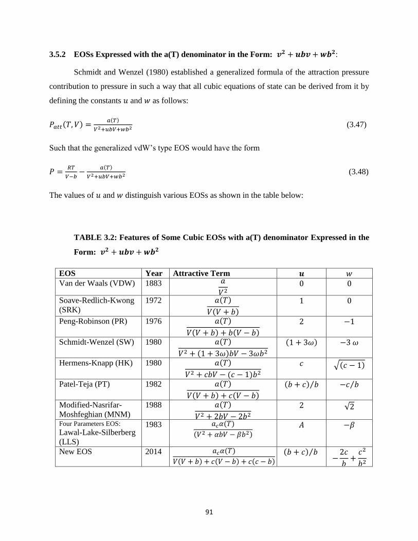
91
3.5.2 EOSs Expressed with the a(T) denominator in the Form: 𝒗𝟐 + 𝒖𝒃𝒗 + 𝒘𝒃𝟐:
Schmidt and Wenzel (1980) established a generalized formula of the attraction pressure
contribution to pressure in such a way that all cubic equations of state can be derived from it by
defining the constants 𝑢 and 𝑤 as follows:
𝑃𝑎𝑡𝑡(𝑇, 𝑉) =𝑎(𝑇)
𝑉2+𝑢𝑏𝑉+𝑤𝑏2 (3.47)
Such that the generalized vdW’s type EOS would have the form
𝑃 =𝑅𝑇
𝑉−𝑏−
𝑎(𝑇)
𝑉2+𝑢𝑏𝑉+𝑤𝑏2 (3.48)
The values of 𝑢 and 𝑤 distinguish various EOSs as shown in the table below:
TABLE 3.2: Features of Some Cubic EOSs with a(T) denominator Expressed in the
Form: 𝒗𝟐 + 𝒖𝒃𝒗 + 𝒘𝒃𝟐
EOS Year Attractive Term 𝒖 𝑤
Van der Waals (VDW) 1883 𝑎
𝑉2 0 0
Soave-Redlich-Kwong
(SRK)
1972 𝑎(𝑇)
𝑉(𝑉 + 𝑏)
1 0
Peng-Robinson (PR) 1976 𝑎(𝑇)
𝑉(𝑉 + 𝑏) + 𝑏(𝑉 − 𝑏)
2 −1
Schmidt-Wenzel (SW) 1980 𝑎(𝑇)
𝑉2 + (1 + 3𝜔)𝑏𝑉 − 3𝜔𝑏2
(1 + 3𝜔) −3 𝜔
Hermens-Knapp (HK) 1980 𝑎(𝑇)
𝑉2 + 𝑐𝑏𝑉 − (𝑐 − 1)𝑏2
𝑐 √(𝑐 − 1)
Patel-Teja (PT) 1982 𝑎(𝑇)
𝑉(𝑉 + 𝑏) + 𝑐(𝑉 − 𝑏)
(𝑏 + 𝑐) 𝑏⁄ −𝑐 𝑏⁄
Modified-Nasrifar-
Moshfeghian (MNM)
1988 𝑎(𝑇)
𝑉2 + 2𝑏𝑉 − 2𝑏2
2 √2
Four Parameters EOS:
Lawal-Lake-Silberberg
(LLS)
1983 𝑎𝑐𝛼(𝑇)
(𝑉2 + 𝛼𝑏𝑉 − 𝛽𝑏2)
𝐴 −𝛽
New EOS 2014 𝑎𝑐𝛼(𝑇)
𝑉(𝑉 + 𝑏) + 𝑐(𝑉 − 𝑏) + 𝑐(𝑐 − 𝑏)
(𝑏 + 𝑐) 𝑏⁄ −
2𝑐
𝑏+
𝑐2
𝑏2
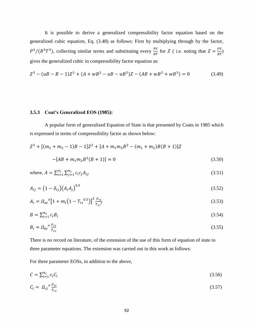
92
It is possible to derive a generalized compressibility factor equation based on the
generalized cubic equation, Eq. (3.48) as follows: First by multiplying through by the factor,
𝑃3 (𝑅3𝑇3)⁄ , collecting similar terms and substituting every 𝑃𝑉
𝑅𝑇 for 𝑍 ( i.e. noting that 𝑍 =
𝑃𝑉
𝑅𝑇)
gives the generalized cubic in compressibility factor equation as:
𝑍3 − (𝑢𝐵 − 𝐵 − 1)𝑍2 + (𝐴 + 𝑤𝐵2 − 𝑢𝐵 − 𝑢𝐵2)𝑍 − (𝐴𝐵 + 𝑤𝐵2 + 𝑤𝐵3) = 0 (3.49)
3.5.3 Coat’s Generalized EOS (1985):
A popular form of generalized Equation of State is that presented by Coats in 1985 which
is expressed in terms of compressibility factor as shown below:
𝑍3 + [(𝑚1 + 𝑚2 − 1)𝐵 − 1]𝑍2 + [𝐴 + 𝑚1𝑚2𝐵2 − (𝑚1 + 𝑚2)𝐵(𝐵 + 1)]𝑍
−[𝐴𝐵 + 𝑚1𝑚2𝐵2(𝐵 + 1)] = 0 (3.50)
where, 𝐴 = ∑ ∑ 𝑐𝑖𝑐𝑗𝐴𝑖𝑗𝑛𝑐𝑗=1
𝑛𝑐𝑖=1 (3.51)
𝐴𝑖𝑗 = (1 − 𝛿𝑖𝑗)(𝐴𝑖𝐴𝑗)0.5
(3.52)
𝐴𝑖 = 𝛺𝑎𝑖𝑜[1 + 𝑚𝑖(1 − 𝑇𝑟𝑖
0.5)]2 𝑃𝑟𝑖
𝑇𝑟𝑖2 (3.53)
𝐵 = ∑ 𝑐𝑖𝐵𝑖𝑛𝑐𝑖=1 (3.54)
𝐵𝑖 = 𝛺𝑏𝑖𝑜 𝑃𝑟𝑖
𝑇𝑟𝑖 (3.55)
There is no record on literature, of the extension of the use of this form of equation of state to
three parameter equations. The extension was carried out in this work as follows:
For three parameter EOSs, in addition to the above,
𝐶 = ∑ 𝑐𝑖𝐶𝑖𝑛𝑐𝑖=1 (3.56)
𝐶𝑖 = 𝛺𝑐𝑖𝑜 𝑃𝑟𝑖
𝑇𝑟𝑖 (3.57)

93
𝑃𝑟𝑖 = 𝑃 𝑃𝑐𝑖⁄ (3.58)
𝑇𝑟𝑖 = 𝑇 𝑇𝑐𝑖⁄ (3.59)
𝛿𝑖𝑗 = 𝑏𝑖𝑛𝑎𝑟𝑦 𝑖𝑛𝑡𝑒𝑟𝑟𝑎𝑐𝑡𝑖𝑜𝑛 𝑐𝑜𝑒𝑓𝑓𝑖𝑐𝑖𝑒𝑛𝑡 𝑜𝑓 𝑡ℎ𝑒 𝑖 − 𝑡ℎ 𝑎𝑛𝑑 𝑗 − 𝑡ℎ 𝑐𝑜𝑚𝑝𝑜𝑛𝑒𝑛𝑡𝑠
Whenever needed, the different equations of state are obtained by substituting the proper
definitions of ′𝑚1′, ′𝑚2′, ′𝛺𝑎𝑖′, 𝛺𝑏𝑖
and ′𝛺𝑐𝑖′, as appropriate for the particular EOS. (Ayala,
2006)
A solution technique requires determining the values of 𝑚1𝑎𝑛𝑑 𝑚2, in particular for each
EOS. This is presented below as Table 3.3 below for some popular EOSs.
TABLE 3.3: Two and Three Parameter EOS Expressed in Form for Use with Coats
(1985) Generalized EOS
EOS 𝒎𝟏 𝒎𝟐 𝜴𝒂𝒊 𝜴𝒃𝒊
𝜴𝒄𝒊
vdW 0 0 0.421875 0.125 ∗
RK 0 1 0.4274802 0.08664035 ∗
SRK 0 1 0.4274802 0.08664035 ∗
PR 1 + √2 1 − √2 0.457235529 0.077796074 ∗
PT (𝑏 + 𝑐
2𝑏)
+1
𝑏√𝑏𝑐 + (
𝑏 + 𝑐
2)
2
(𝑏 + 𝑐
2𝑏)
−1
𝑏√𝑏𝑐 + (
𝑏 + 𝑐
2)
2
∗∗ ∗∗ ∗∗
NEW (𝑏 + 𝑐
2𝑏)
+1
𝑏√2𝑏𝑐 − 𝑐2 + (
𝑏 + 𝑐
2)
2
(𝑏 + 𝑐
2𝑏)
−1
𝑏√2𝑏𝑐 − 𝑐2 + (
𝑏 + 𝑐
2)
2
∗∗ ∗∗ ∗∗
∗ These values do not exist for the associated equations of state.
∗∗ For the EOS parameters marked with these, Ω𝑎, Ω𝑏and Ω𝑐 are calculated as follows:

94
Ω𝑏is smallest root of the equation:
Ω𝑏3 + (2 − 3𝜉𝑐)Ω𝑏
2 + 3𝜉𝑐2Ω𝑏 − 𝜉𝑐
3 = 0. (3.60)
Ω𝑐 = 1 − 3𝜉𝑐 and (3.61)
Ω𝑎 = 3𝜉𝑐2 + 3(1 − 2𝜉𝑐)Ω𝑏 + Ω𝑏
2 + (1 − 3𝜉𝑐) (3.62)
𝜉𝑐 = 0.329032 − 0.0767992𝜔 + 0.0211947𝜔2 (3.63)
In terms of fugacity coefficient, Equation (3.50) can be written as:
ln 𝜙𝑖 = −𝑙𝑛(𝑍 − 𝐵) +𝐴
(𝑚1−𝑚2)𝐵[
2 ∑ 𝐴𝑖𝑗𝑐𝑗𝑛𝑐𝑗=1
𝐴−
𝐵𝑖
𝐵] 𝑙𝑛 [
𝑍+𝑚2𝐵
𝑍+𝑚1𝐵] +
𝐵𝑖
𝐵(𝑍 − 1) (3.64)
Where : 𝜙𝑖 = 𝑓𝑢𝑔𝑎𝑐𝑖𝑡𝑦 𝑐𝑜𝑒𝑓𝑓𝑖𝑐𝑖𝑒𝑛𝑡 𝑜𝑓 𝑡ℎ𝑒 𝑖 − 𝑡ℎ 𝑐𝑜𝑚𝑝𝑜𝑛𝑒𝑛𝑡 (𝑑𝑖𝑚𝑒𝑛𝑠𝑖𝑜𝑛𝑙𝑒𝑠𝑠)
For the liquid phase, eqn. (3.64) is adaptable to the form:
𝜙𝑙𝑖= 𝐴𝐿𝑂𝐺 [−𝑙𝑛(𝑍𝑙 − 𝐵) +
𝐴
(𝑚1−𝑚2)𝐵[
2 ∑ 𝐴𝑖𝑗𝑥𝑖𝑛𝑐𝑖=1
𝐴−
𝐵𝑖
𝐵] 𝑙𝑛 [
𝑍𝑙+𝑚2𝐵
𝑍𝑙+𝑚1𝐵] +
𝐵𝑖
𝐵(𝑍𝑙 − 1)] (3.65)
and for the gas phase,
𝜙𝑔𝑖= 𝐴𝐿𝑂𝐺 [−𝑙𝑛(𝑍𝑔 − 𝐵) +
𝐴
(𝑚1−𝑚2)𝐵[
2 ∑ 𝐴𝑖𝑗𝑦𝑖𝑛𝑐𝑖=1
𝐴−
𝐵𝑖
𝐵] 𝑙𝑛 [
𝑍𝑔+𝑚2𝐵
𝑍𝑔+𝑚1𝐵] +
𝐵𝑖
𝐵(𝑍𝑔 − 1)] (3.66)
When expressed in the form of Coats (1985) generalized equation of state, the New
EOS has the form:
𝑍3 + (𝐶 − 1)𝑍2 + (𝐴 − 𝐵 − 𝐶 − 3𝐵𝐶 − 𝐵2 + 𝐶2)𝑍 + (2𝐵𝐶 + 2𝐵2𝐶 − 𝐵𝐶2 − 𝐶2 − 𝐴𝐵) = 0 (3.67)
3.6 Expressing Cubic Equations of State (CEOSs) in Terms of Virial Coefficients

95
The repulsion part of any van der Waal type equation of state has the same form of the
repulsion term which can be written as:
𝑅𝑇
𝑉−𝑏=
𝑅𝑇
𝑉(
1
1−𝑏 𝑉⁄) =
𝑅𝑇
𝑉[1 +
𝑏
𝑉+
𝑏2
𝑉2 +𝑏3
𝑉3 +. . . ] (3.68)
The second (attraction) term may be written as:
𝑎
𝑉2+𝑢𝑏𝑉+𝑤𝑏2=
𝑎
𝑉[
1
𝑉+𝑢𝑏+(𝑤𝑏2 𝑉⁄ )] =
𝑎
𝑉[
1
𝑉−
𝑢𝑏
𝑉2+
(𝑢2−𝑤)𝑏2
𝑉3+ . . . ] (3.69)
Therefore, the generalized EOS may be written in terms of Eqs. (3.68) and (3.69) as:
𝑃 =𝑅𝑇
𝑉[1 +
𝑏
𝑉+
𝑏2
𝑉2 +𝑏3
𝑉3 +. . . ] −𝑎
𝑉[
1
𝑉−
𝑢𝑏
𝑉2 +(𝑢2−𝑤)𝑏2
𝑉3 + . . . ] (3.70)
Noting that, 𝑍 =𝑃𝑉
𝑅𝑇, multiplying Eq. (3.70) through by
𝑉
𝑅𝑇 and collecting like terms gives the following:
𝑍 = 1 + [𝑏 −𝑎
𝑅𝑇]
1
𝑉+ [𝑏2 +
𝑢𝑎𝑏
𝑅𝑇]
1
𝑉2 + [𝑏3 +(𝑤−𝑢2)𝑎𝑏2
𝑅𝑇]
1
𝑉3 + . . . (3.71)
It is important to note that virial equations of state express the compressibility coefficient
by expansion in a power series in terms of density, 𝜌 or as a development in terms of pressure:
𝑍 =𝑃𝑉
𝑅𝑇= 1 + 𝐵𝜌 + 𝐶𝜌2 + 𝐷𝜌3 + ⋯ = 1 + 𝐵′𝑃 + 𝐶′𝑃2 + 𝐷′𝑃3 + ⋯ (3.72a)
Or 𝑍 =𝑃𝑉
𝑅𝑇= 1 +
𝐵
𝑉+
𝐶
𝑉2 +𝐷
𝑉3 + ⋯ (3.72b)
Where, coefficients 𝐵, 𝐶, 𝐷 𝑜𝑟 𝐵′, 𝐶′, 𝐷′, 𝑒𝑡𝑐., are called the 𝑠𝑒𝑐𝑜𝑛𝑑, 𝑡ℎ𝑖𝑟𝑑, 𝑓𝑜𝑢𝑟𝑡ℎ, 𝑒𝑡𝑐. virial
coefficients respectively. 𝐵 corresponds to interactions between pairs of molecules, 𝐶 to triplets,
𝐷 to four molecular interactions and so on. Accuracy can be increased indefinitely by
considering higher orders, however, they can be truncated at the second virial coefficient at
moderate to low pressures without significantly impacting accuracy. Virial coefficients are
functions of temperature only.
By comparing Eq. (3.71) to Eq. (3.72b), the virial coefficients could be obtained by
comparing coefficients, such that,
The second virial coefficient would be, 𝐵 = 𝑏 −𝑎
𝑅𝑇 (3.73)
The third virial coefficient would be, 𝐶 = 𝑏2 +𝑢𝑎𝑏
𝑅𝑇 (3.74)
The fourth virial coefficient would be,
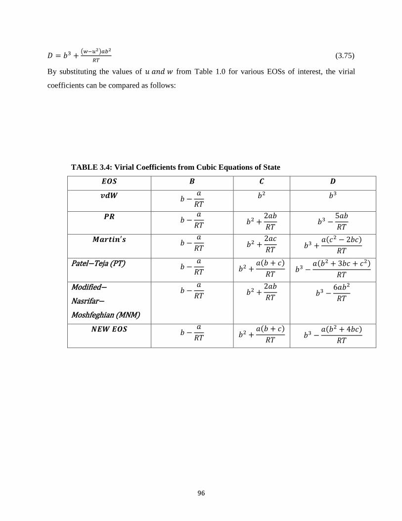
96
𝐷 = 𝑏3 +(𝑤−𝑢2)𝑎𝑏2
𝑅𝑇 (3.75)
By substituting the values of 𝑢 𝑎𝑛𝑑 𝑤 from Table 1.0 for various EOSs of interest, the virial
coefficients can be compared as follows:
TABLE 3.4: Virial Coefficients from Cubic Equations of State
𝑬𝑶𝑺 𝑩 𝑪 𝑫
𝒗𝒅𝑾 𝑏 −𝑎
𝑅𝑇 𝑏2 𝑏3
𝑷𝑹 𝑏 −𝑎
𝑅𝑇 𝑏2 +
2𝑎𝑏
𝑅𝑇 𝑏3 −
5𝑎𝑏
𝑅𝑇
𝑴𝒂𝒓𝒕𝒊𝒏′𝒔 𝑏 −𝑎
𝑅𝑇 𝑏2 +
2𝑎𝑐
𝑅𝑇 𝑏3 +
𝑎(𝑐2 − 2𝑏𝑐)
𝑅𝑇
Patel−Teja (PT) 𝑏 −𝑎
𝑅𝑇 𝑏2 +
𝑎(𝑏 + 𝑐)
𝑅𝑇 𝑏3 −
𝑎(𝑏2 + 3𝑏𝑐 + 𝑐2)
𝑅𝑇
Modified−
Nasrifar−
Moshfeghian (MNM)
𝑏 −𝑎
𝑅𝑇 𝑏2 +
2𝑎𝑏
𝑅𝑇 𝑏3 −
6𝑎𝑏2
𝑅𝑇
𝑵𝑬𝑾 𝑬𝑶𝑺 𝑏 −𝑎
𝑅𝑇 𝑏2 +
𝑎(𝑏 + 𝑐)
𝑅𝑇 𝑏3 −
𝑎(𝑏2 + 4𝑏𝑐)
𝑅𝑇
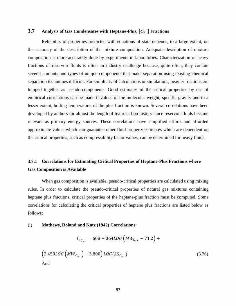
97
3.7 Analysis of Gas Condensates with Heptane-Plus, [𝑪𝟕+] Fractions
Reliability of properties predicted with equations of state depends, to a large extent, on
the accuracy of the description of the mixture composition. Adequate description of mixture
composition is more accurately done by experiments in laboratories. Characterization of heavy
fractions of reservoir fluids is often an industry challenge because, quite often, they contain
several amounts and types of unique components that make separation using existing chemical
separation techniques difficult. For simplicity of calculations or simulations, heavier fractions are
lumped together as pseudo-components. Good estimates of the critical properties by use of
empirical correlations can be made if values of the molecular weight, specific gravity and to a
lesser extent, boiling temperature, of the plus fraction is known. Several correlations have been
developed by authors for almost the length of hydrocarbon history since reservoir fluids became
relevant as primary energy sources. These correlations have simplified efforts and afforded
approximate values which can guarantee other fluid property estimates which are dependent on
the critical properties, such as compressibility factor values, can be determined for heavy fluids.
3.7.1 Correlations for Estimating Critical Properties of Heptane-Plus Fractions where
Gas Composition is Available
When gas composition is available, pseudo-critical properties are calculated using mixing
rules. In order to calculate the pseudo-critical properties of natural gas mixtures containing
heptane plus fractions, critical properties of the heptane-plus fraction must be computed. Some
correlations for calculating the critical properties of heptane plus fractions are listed below as
follows:
(i) Mathews, Roland and Katz (1942) Correlations:
𝑇𝑐𝐶7+
= 608 + 364𝐿𝑂𝐺 (𝑀𝑊𝐶7+ − 71.2) +
(2,450𝐿𝑂𝐺 (𝑀𝑊𝐶7+ ) − 3,800) 𝐿𝑂𝐺(𝑆𝐺𝐶
7+ ) (3.76)
And

98
𝑃𝑐𝐶7+
= 1,188 − 431𝐿𝑂𝐺 (𝑀𝑊𝐶7+ − 61.1) + [2,319 − 852𝐿𝑂𝐺 (𝑀𝑊𝐶
7+ −
53.7)] (𝑆𝐺𝐶7+ − 0.8) (3.77)
(ii) Standing’s (1981) representation of the graphical correlation of Mathews et al. (1942):
𝑇𝑐𝐶7+
= 338 + 202 ∗ 𝐿𝑂𝐺 (𝑀𝑊𝐶7+ − 71.2) + (1361 ∗ 𝐿𝑂𝐺 (𝑀𝑊𝐶
7+) − 2111) ∗
𝐿𝑂𝐺(𝑆𝐺𝐶7+) (3.78)
𝑃𝑐𝐶7+
= 8.191 − 2.97 ∗ 𝐿𝑂𝐺 (𝑀𝑊𝐶7+ − 61.1) + (𝑆𝐺𝐶
7+ − 0.8) ∗ [15.99 − 5.87 ∗
𝐿𝑂𝐺 (𝑀𝑊𝐶7+ − 53.7)] (3.79)
Where, 𝑇𝑐 and 𝑃𝑐 are in 𝐾𝑒𝑙𝑣𝑖𝑛 [𝐾] and 𝑀𝑃𝑎, respectively.
(iii) Kesler-Lee Correlation: Kesler and Lee (1976) developed the following correlation:
𝑇𝑐𝐶7+
= 341.7 + 811.1 ∗ 𝑆𝐺𝐶7+ + (0.4244 + 0.1174 ∗ 𝑆𝐺𝐶
7+) ∗ 𝑇𝑏 + (0.4669 − 3.26238 ∗
𝑆𝐺𝐶7+ ) ∗
105
𝑇𝑏 (3.80)
𝑙𝑛 (𝑃𝑐𝐶7+
) = 8.3634 −0.0566
𝑆𝐺𝐶7+
− (0.24444 +2.2898
𝑆𝐺𝐶7+
+0.11857
(𝑆𝐺𝐶7+ )
2) ∗ 10−3 ∗ 𝑇𝑏 + (1.4685 +
3.648
𝑆𝐺𝐶7+
+0.47227
(𝑆𝐺𝐶7+)
2) ∗ 10−7 ∗ (𝑇𝑏)2 − (0.42019 +1.6977
(𝑆𝐺𝐶7+ )
2) ∗ 10−10 ∗ (𝑇𝑏)3 (3.81)
The Kesler-lee method correlates critical properties as functions of boiling point and specific
gravity. The boiling point parameter,(𝑇𝑏) , can be estimated from Whitson’s correlation:
𝑇𝑏 = (4.5579 ∗ (𝑀𝑊𝐶7+ )
0.15178
∗ (𝑆𝐺𝐶7+)
0.15427
)3
(3.82)
99
(iv) Winn-Sim-Daubert Correlation (1980): This correlation has the forms:
𝑇𝑐𝐶7+ = 𝐸𝑋𝑃 [3.994718 ∗ 𝑇𝑏
0.08615 ∗ (𝑆𝐺𝐶7+ )
0.04614
] (3.83)
𝑃𝑐𝐶7+
= 3.48242 ∗ 109 ∗ 𝑇𝑏−2.3177 ∗ (𝑆𝐺𝐶
7+ )2.4853
(3.84)
𝑊ℎ𝑒𝑟𝑒, 𝑇𝑏𝑖𝑠 𝑡ℎ𝑒 𝑏𝑜𝑖𝑙𝑖𝑛𝑔 𝑝𝑜𝑖𝑛𝑡 𝑖𝑛 𝑅𝑜
(v) Piper et al. correlation (1993):
Piper et al.(1993) developed two separate equations depending on whether the composition or
the specific gravity is known. Where the gas compositions are known, the following equations
are used:
𝐽 = 𝛼0 + ∑ 𝛼𝑖 (𝑦𝑖𝑇𝑐𝑖
𝑃𝑐𝑖) + 𝛼4 ∑ 𝑦𝑗 (
𝑇𝑐𝑗
𝑃𝑐𝑗) + 𝛼6𝑦𝐶7+
𝑀𝐶7+
6𝑗=1 + 𝛼7(𝑦𝐶7+
𝑀𝐶7+)
23𝑖=1 (3.85)
𝐾 = 𝛽0 + ∑ 𝛽𝑖 (𝑦𝑖𝑇𝑐𝑖
√𝑃𝑐𝑖)3
𝑖=1 + 𝛽4 ∑ 𝑦𝑗6𝑗=1 (
𝑇𝑐𝑗
√𝑃𝑐𝑗) + 𝛽6𝑦𝐶7+
𝑀𝐶7++ 𝛽7(𝑦𝐶7+
𝑀𝐶7+)
2 (3.86)
Where, 𝑦𝑖 are the contaminant compositions 𝑦𝐻2𝑆, 𝑦𝐶𝑂2, 𝑦𝑁2
, and 𝑦𝑗 are the hydrocarbon
compositions 𝑦𝐶1, 𝑦𝐶2
, 𝑦𝐶3, 𝑦𝐶4
, 𝑦𝐶5, 𝑦𝐶6
.
Then the final pseudo reduced properties (𝑃𝑟𝑎𝑛𝑑 𝑇𝑟) are calculates as follows:
𝑃𝑟 =𝑃
𝑃𝑝𝑐′ and 𝑇𝑟 =
𝑇
𝑇𝑝𝑐′.
𝛼 𝑎𝑛𝑑 𝛽 are as given in table below.

100
TABLE 3.5. VALUES OF 𝜶𝒊 𝒂𝒏𝒅 𝜷𝒊 for Piper et al. (1993) Correlation
𝑖 𝛼𝑖 𝛽𝑖
0 0.052073 -0.39741
1 1.0160 1.0503
2 0.86961 0.96592
3 0.72646 0.78569
4 0.85101 0.98211
5 0.0 0.0
6 0.020818 0.45536
7 -0.0001506 -0.0037684
(vi) Watansiri-Owens-Starling Correlation (1985): The correlation of Watansiri, Owens
and Starling is as shown below:
𝑙𝑛 (𝑇𝑐𝐶7+
) = −0.0650504 − 0.0005217 ∗ 𝑇𝑏 + 0.03905 ∗ 𝑙𝑛 (𝑀𝑊𝐶7+ ) +
1.11067 ∗ 𝑙𝑛(𝑇𝑏) ∗ (𝑀𝑊𝐶7+ ) ∗ [0.078154 ∗ (𝑆𝐺𝐶
7+ )1 2⁄
− 0.061061 ∗
(𝑆𝐺𝐶7+ )
1 3⁄
− 0.016943 ∗ 𝑆𝐺𝐶7+ ] (3.87)
𝑙𝑛 (𝑃𝑐𝐶7+
) = 6.6418853 + 0.01617283 ∗ (𝑇𝑐𝐶
7+
𝑉𝑐𝐶7+
)
0.8
− 8.712 ∗ (𝑀𝑊𝐶
7+
𝑇𝑐𝐶7+
) −
0.08843889 ∗ (𝑇𝑏
𝑀𝑊𝐶7+
) (3.88)
Where, 𝑙𝑛 (𝑉𝑐𝐶7+
) = 76.313887 − 129.8038 ∗ 𝑆𝐺𝐶7+ + 63.175 ∗ (𝑆𝐺𝐶
7+ )2
−
13.175 ∗ (𝑆𝐺𝐶7+ )
3
+ 1.10108 ∗ 𝑙𝑛 (𝑀𝑊𝐶7+ ) + 42.1958 ∗ 𝑙𝑛 (𝑆𝐺𝐶
7+ ) (3.89)
(vii) Riazi-Daubert Correlation (1987): Riazi and Daubert established and presented the
following correlations for critical properties and boiling temperature in 1987:
𝜃 = 𝑎 ∗ 𝑀𝑊𝑏 ∗ 𝑆𝐺𝑐 ∗ 𝐸𝑋𝑃[𝑑 ∗ 𝑀𝑊 + 𝑒 ∗ 𝑆𝐺 + 𝑓 ∗ (𝑀𝑊 ∗ 𝑆𝐺)]
Where, 𝜃 = some physical property
𝑎 − 𝑓 = coefficients for each physical property (See Table below).

101
TABLE 3.6: Riazi and Daubert’s Coefficients
𝜃 𝑇𝑐 𝑃𝑐 𝑇𝑏
𝑎 544.4 45203 6.77857
𝑏 0.2998 -0.8063 0.401673
𝑐 1.0555 1.6015 -1.58262
𝑑 -0.00013478 -0.0018078 0.00377409
𝑒 -0.61641 -0.3084 2.984036
𝑓 0.000000 0.000000 -0.00425288
A comparative study of these various correlations showed that the Riazi-Daubert
correlation is simple to apply, results need no further conversions to field units and are accurate
over a wider range of gas gravities than others studied. However, its performance, especially for
critical pressure estimation, is compromised in the range: 0.770 ≤ 𝑆𝐺𝐶7+ ≤ 0.850 .
A new correlation to use in this specific gravity range to ameliorate the shortcomings is
presented as:
𝑃𝑐𝐶7+
= 251.6 + 0.135 ∗ 𝐿𝑂𝐺 (𝑀𝑊𝐶7+ ) + 0.101 ∗ 𝑆𝐺𝐶
7+ + 0.976 ∗ 𝑀𝑊𝐶7+ ∗ (𝑆𝐺𝐶
7+)0.0125
(3.90)

102
3.7.2 Correlations for Estimating Critical Properties of Heptane Plus Fractions where
Gas Composition is Unavailable
When gas composition is not available, critical property correlations are often based on
gas gravities and molecular weights and in some cases on boiling point temperatures in addition.
Some correlations which fall into this category as listed below:
(i) Standing’s correlation (1981):
Standing, based on work on light molecular weight California natural gases presented
two sets of correlations: one for
Dry hydrocarbon gases (𝜸𝒈 < 𝟎. 𝟕𝟓):
𝑇𝑝𝑐 = 168 + 325𝛾𝑔 − 12.5𝛾𝑔2 (3.91)
and 𝑃𝑝𝑐 = 667 + 15.0𝛾𝑔 − 37.5𝛾𝑔2 (3.92)
and one for wet gas mixtures (𝜸𝒈 ≥ 𝟎. 𝟕𝟓):
𝑇𝑝𝑐 = 187 + 330𝛾𝑔 − 71.5𝛾𝑔2 (3.93)
And 𝑃𝑝𝑐 = 706 − 51.7𝛾𝑔 − 11.1𝛾𝑔2 (3.94)
Standing indicated that his correlation works only when there is no non-hydrocarbon gases
present in the natural gas mixture.
(ii) Sutton’s (1985) Correlation:
Sutton, working with PVT reports of high molecular weight, mainly sweet gases rich in
Heptane-plus fractions, developed the following correlations:
𝑃𝑝𝑐 = 756.8 − 131.07𝛾𝑔 − 3.6𝛾𝑔2 (3.95)
and 𝑇𝑝𝑐 = 169.2 + 349.5𝛾𝑔 − 74.0𝛾𝑔2 (3.96)

103
Sutton developed his correlation using gases which had minor amounts of carbon dioxide
and nitrogen with no hydrogen sulfide. The range of the gas gravities were 0.57 < 𝛾𝑔 < 1.68.
Thomas et al. (1970), recommended the use of these equations in allowable limits of up to
3% 𝐻2𝑆 , 5% 𝑁2, or a total impurity (non-hydrocarbon) content of 7%, beyond which errors in
critical pressures exceed 6%.
(iii) Elsharkawy et al.’s (2004) Correlation:
Elsharkawy et al.(2004) developed a correlation for critical properties using a large data
bank of retrograde gas condensates with minor amounts of hydrogen sulfide. The correlation has
the form:
𝑃𝑝𝑐 = 787.06 − 147.34𝛾𝑔 − 7.916𝛾𝑔2 (3.97)
and 𝑇𝑝𝑐 = 149.18 + 358.14𝛾𝑔 − 66.976𝛾𝑔2 (3.98)
(iv) Piper et al. (1993 ) Correlation:
If the composition of the hydrocarbons is not known but the specific gravity and the non-
hydrocarbon compositions are known, the following equations for 𝐽 𝑎𝑛𝑑 𝐾 were developed
by Piper et al., on the basis of 1,482 data points:
𝐽 = 0.11582 − 0.4582𝑦𝐻2𝑆 (𝑇𝑐
𝑃𝑐)
𝐻2𝑆− 0.90348𝑦𝐶𝑂2
(𝑇𝑐
𝑃𝑐)
𝐶𝑂2
− 0.66026 (𝑇𝑐
𝑃𝑐)
𝑁2
+
0.70729𝛾𝑔 − 0.099397𝛾𝑔2 (3.99)
𝐾 = 3.8216 − 0.06534𝑦𝐻2𝑆 (𝑇𝑐
√𝑃𝑐
)
𝐻2𝑆
− 0.42113𝑦𝐶𝑂2(
𝑇𝑐
√𝑃𝑐
)
𝐶𝑂2
−0.91249𝑦𝑁2(
𝑇𝑐
√𝑃𝑐)
𝑁2
+ 17.438𝛾𝑔 − 3.2191𝛾𝑔2 (3.100)
Then, the pseudocritical properties can be calculated from:
104
𝑇𝑝𝑐 =𝐾2
𝐽 (3.101)
and 𝑃𝑝𝑐 =𝑇𝑝𝑐
𝐽 (3.102)
3.8 Analysis of Gas Condensates Containing Acid Gases
Wichert and Aziz (1972) Correlation: The presence of acid gases in gas mixtures often
distorts accuracy as most models were developed for strictly hydrocarbon fractions. Wichert and
Aziz (1972) developed a correlation to account for inaccuracies due to the presence of acid gases
(carbon dioxide, (𝐶𝑂2) and hydrogen sulfide, (𝐻2𝑆). The Wichert and Aziz correlation first
calculates a deviation parameter, 휀, given by:
휀 = 120 ∗ (𝐴0.9 − 𝐴1.6) + 15 ∗ (𝐵0.5 − 𝐵4) (3.103)
Where, 𝐴 = the sum of the mole fractions of 𝐶𝑂2 and 𝐻2𝑆 in the gas mixture and 𝐵 = the mole
fraction of 𝐻2𝑆 alone, in the gas mixture. The value of 휀 is used to modify the values of the
pseudo critical temperature and pressure as follows:
𝑇𝑝𝑐′ = 𝑇𝑝𝑐 − 휀 (3.104)
And
𝑃𝑝𝑐′ =
𝑃𝑝𝑐𝑇𝑝𝑐′
𝑇𝑝𝑐−𝐵(1−𝐵)𝜀 . (3.105)
If only gas gravity and non-hydrocarbon content are known, the hydrocarbon specific gravity is
first calculated from:
𝛾𝑔𝐻𝐶=
𝛾𝑔−(𝑦𝑁2𝑀𝑊𝑁2+𝑦𝐶𝑂2𝑀𝑊𝐶𝑂2+𝑦𝐻2𝑆𝑀𝑊𝐻2𝑆) 𝑀𝑊𝑎𝑖𝑟⁄
1−𝑦𝑁2−𝑦𝐶𝑂2−𝑦𝐻2𝑆 (3.106)
Hydrocarbon pseudo-critical properties are then calculated from Sutton’s correlation and
adjusted for non-hydrocarbon content on the basis of Kay’s mixing rule:

105
𝑃𝑝𝑐∗ = (1 − 𝑦𝑁2
− 𝑦𝐶𝑂2− 𝑦𝐻2𝑆)𝑃𝑝𝑐𝐻𝐶
+ 𝑦𝑁2𝑃𝑐𝑁2
+ 𝑦𝐶𝑂2𝑃𝑐𝐶𝑂2
+ 𝑦𝐻2𝑆𝑃𝑐𝐻2𝑆 (3.107)
And 𝑇𝑝𝑐∗ = (1 − 𝑦𝑁2
− 𝑦𝐶𝑂2− 𝑦𝐻2𝑆)𝑇𝑝𝑐𝐻𝐶
+ 𝑦𝑁2𝑇𝑐𝑁2
+ 𝑦𝐶𝑂2𝑇𝑐𝐶𝑂2
+ 𝑦𝐻2𝑆𝑇𝑐𝐻2𝑆 (3.108)
𝑃𝑝𝑐∗ and 𝑇𝑝𝑐
∗ are used in the Wichert-Aziz equations with hydrogen sulfide and carbon dioxide
mole fractions to obtain mixture 𝑃𝑝𝑐 and 𝑇𝑝𝑐, respectively.
The correlations are valid for concentrations of 𝐶𝑂2 < 54.4 𝑚𝑜𝑙% and 𝐻2𝑆 < 73.8%.
𝑇𝑝𝑐′, 𝑇𝑝𝑐 𝑎𝑛𝑑 휀 have units of Rankine while 𝑃𝑝𝑐
′ and 𝑃𝑝𝑐 are in pounds per square inch absolute,
𝑝𝑠𝑖𝑎.
The final pseudo reduced properties (𝑃𝑟𝑎𝑛𝑑 𝑇𝑟) are calculates as follows:
𝑃𝑟 =𝑃
𝑃𝑝𝑐′ (3.109)
and 𝑇𝑟 =𝑇
𝑇𝑝𝑐′. (3.110)

106
CHAPTER FOUR
4.0 RESULTS AND DISCUSSION OF RESULTS
This chapter is primarily devoted to comparing the performance of the New equation of
state with that of the industry popular two parameter Peng-Robinson’s and three parameter
Patel-Teja’s equations of state using experimentally measured thermodynamic properties data
from literature. The comparisons were carried out for predictions of thermodynamic properties of
gas and liquid phase single component and multi-component systems. The multicomponent
systems compositions varied in terms of number of components in the mixture as well as in
amounts of constituents of the mixtures.
The development of a quintessential equation of state, for which minimal error is incurred
in its use for predicting thermodynamic properties when compared to experimentally measured
values, would be of immense importance to Petroleum and Chemical engineers who constantly
involved in fluid properties estimations and use on an almost daily basis. Bearing this in mind, it
can be said that every effort that minimizes existing gap between equation of state-derived and
experimentally-calculated properties is a welcome and laudable contribution to the field of fluid
engineering. The new equation of state presented, is promising enough in that it consistently
excels in the minimization of bias, on the average, for equation of state calculated
thermodynamic properties in comparison to experimentally derived measurements of similar
properties. The performance of the New equation of state is compared to those of two popular
equations of state in the industry, namely, the two parameter Peng-Robinson’s equation of state
and the three parameter Patel-Teja’s equation of state. The results of these comparisons are
discussed below.
4.1 Application to Single Component Systems
Most equations of state give fairly accurate predictions of vapor molar volumes but fail
significantly in predicting liquid densities to a good degree of accuracy. Liquid densities have
therefore; become an acid test for measuring equation of state capabilities. Tables 4.1 below
show performances of the new equation of state in predicting liquid densities for pure substances
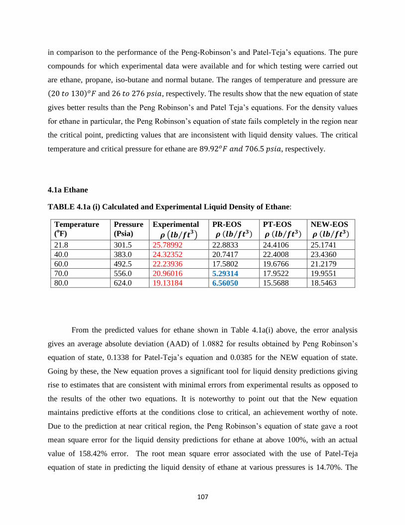
107
in comparison to the performance of the Peng-Robinson’s and Patel-Teja’s equations. The pure
compounds for which experimental data were available and for which testing were carried out
are ethane, propane, iso-butane and normal butane. The ranges of temperature and pressure are
(20 𝑡𝑜 130)𝑜𝐹 and 26 𝑡𝑜 276 𝑝𝑠𝑖𝑎, respectively. The results show that the new equation of state
gives better results than the Peng Robinson’s and Patel Teja’s equations. For the density values
for ethane in particular, the Peng Robinson’s equation of state fails completely in the region near
the critical point, predicting values that are inconsistent with liquid density values. The critical
temperature and critical pressure for ethane are 89.92𝑜𝐹 𝑎𝑛𝑑 706.5 𝑝𝑠𝑖𝑎, respectively.
4.1a Ethane
TABLE 4.1a (i) Calculated and Experimental Liquid Density of Ethane:
Temperature
(oF)
Pressure
(Psia)
Experimental
𝝆 (𝒍𝒃 𝒇𝒕𝟑⁄ )
PR-EOS
𝝆 (𝒍𝒃 𝒇𝒕𝟑⁄ )
PT-EOS
𝝆 (𝒍𝒃 𝒇𝒕𝟑⁄ )
NEW-EOS
𝝆 (𝒍𝒃 𝒇𝒕𝟑⁄ )
21.8 301.5 25.78992 22.8833 24.4106 25.1741
40.0 383.0 24.32352 20.7417 22.4008 23.4360
60.0 492.5 22.23936 17.5802 19.6766 21.2179
70.0 556.0 20.96016 5.29314 17.9522 19.9551
80.0 624.0 19.13184 6.56050 15.5688 18.5463
From the predicted values for ethane shown in Table 4.1a(i) above, the error analysis
gives an average absolute deviation (AAD) of 1.0882 for results obtained by Peng Robinson’s
equation of state, 0.1338 for Patel-Teja’s equation and 0.0385 for the NEW equation of state.
Going by these, the New equation proves a significant tool for liquid density predictions giving
rise to estimates that are consistent with minimal errors from experimental results as opposed to
the results of the other two equations. It is noteworthy to point out that the New equation
maintains predictive efforts at the conditions close to critical, an achievement worthy of note.
Due to the prediction at near critical region, the Peng Robinson’s equation of state gave a root
mean square error for the liquid density predictions for ethane at above 100%, with an actual
value of 158.42% error. The root mean square error associated with the use of Patel-Teja
equation of state in predicting the liquid density of ethane at various pressures is 14.70%. The
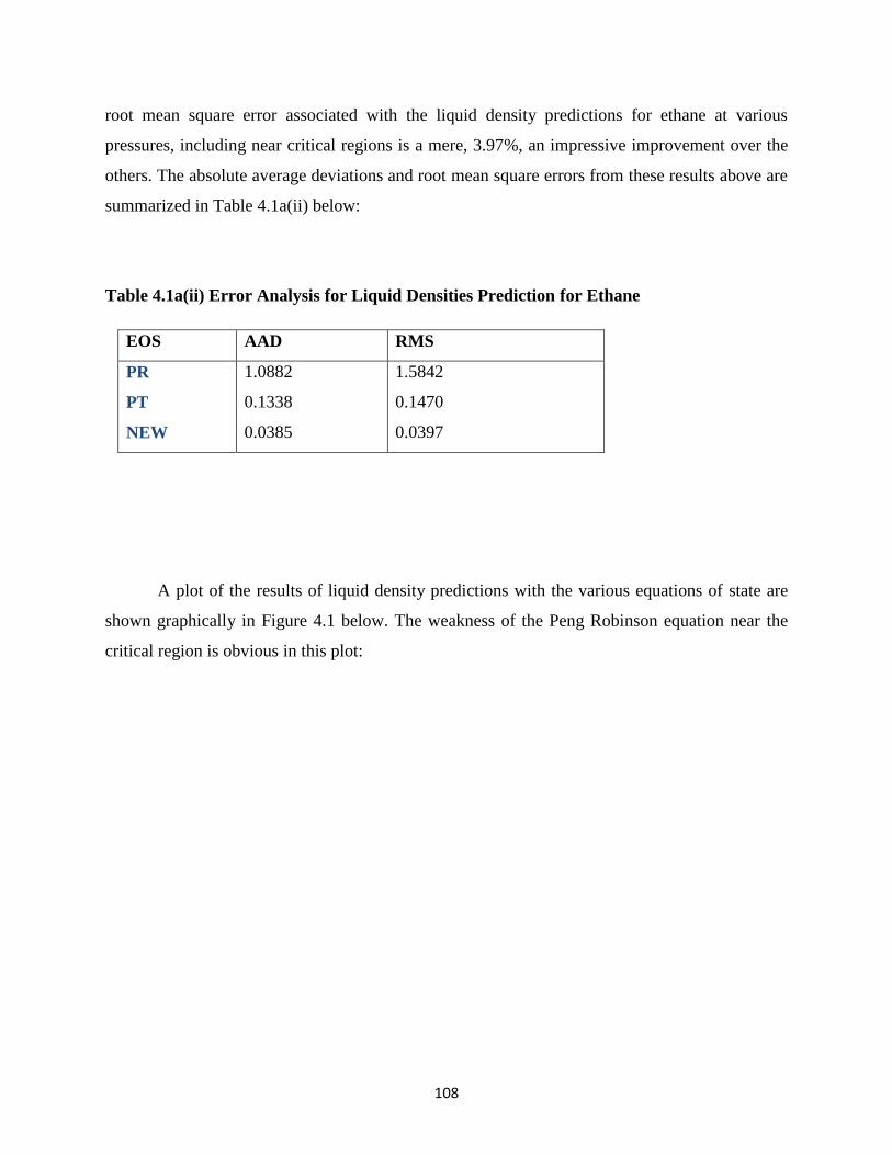
108
root mean square error associated with the liquid density predictions for ethane at various
pressures, including near critical regions is a mere, 3.97%, an impressive improvement over the
others. The absolute average deviations and root mean square errors from these results above are
summarized in Table 4.1a(ii) below:
Table 4.1a(ii) Error Analysis for Liquid Densities Prediction for Ethane
EOS AAD RMS
PR
PT
NEW
1.0882
0.1338
0.0385
1.5842
0.1470
0.0397
A plot of the results of liquid density predictions with the various equations of state are
shown graphically in Figure 4.1 below. The weakness of the Peng Robinson equation near the
critical region is obvious in this plot:
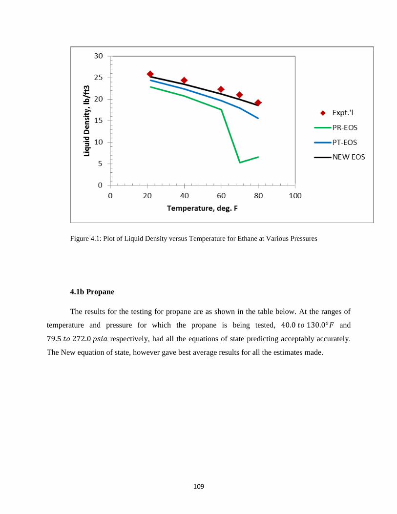
109
Figure 4.1: Plot of Liquid Density versus Temperature for Ethane at Various Pressures
4.1b Propane
The results for the testing for propane are as shown in the table below. At the ranges of
temperature and pressure for which the propane is being tested, 40.0 𝑡𝑜 130.0𝑜𝐹 and
79.5 𝑡𝑜 272.0 𝑝𝑠𝑖𝑎 respectively, had all the equations of state predicting acceptably accurately.
The New equation of state, however gave best average results for all the estimates made.
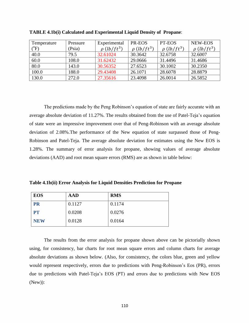
110
TABLE 4.1b(i) Calculated and Experimental Liquid Density of Propane:
Temperature
(oF)
Pressure
(Psia)
Experimental
𝜌 (𝑙𝑏 𝑓𝑡3⁄ )
PR-EOS
𝜌 (𝑙𝑏 𝑓𝑡3⁄ )
PT-EOS
𝜌 (𝑙𝑏 𝑓𝑡3⁄ )
NEW-EOS
𝜌 (𝑙𝑏 𝑓𝑡3⁄ )
40.0 79.5 32.61024 30.3642 32.6758 32.6007
60.0 108.0 31.62432 29.0666 31.4496 31.4686
80.0 143.0 30.56352 27.6523 30.1002 30.2350
100.0 188.0 29.43408 26.1071 28.6078 28.8879
130.0 272.0 27.35616 23.4098 26.0014 26.5852
The predictions made by the Peng Robinson’s equation of state are fairly accurate with an
average absolute deviation of 11.27%. The results obtained from the use of Patel-Teja’s equation
of state were an impressive improvement over that of Peng-Robinson with an average absolute
deviation of 2.08%.The performance of the New equation of state surpassed those of Peng-
Robinson and Patel-Teja. The average absolute deviation for estimates using the New EOS is
1.28%. The summary of error analysis for propane, showing values of average absolute
deviations (AAD) and root mean square errors (RMS) are as shown in table below:
Table 4.1b(ii) Error Analysis for Liquid Densities Prediction for Propane
EOS AAD RMS
PR
PT
NEW
0.1127
0.0208
0.0128
0.1174
0.0276
0.0164
The results from the error analysis for propane shown above can be pictorially shown
using, for consistency, bar charts for root mean square errors and column charts for average
absolute deviations as shown below. (Also, for consistency, the colors blue, green and yellow
would represent respectively, errors due to predictions with Peng-Robinson’s Eos (PR), errors
due to predictions with Patel-Teja’s EOS (PT) and errors due to predictions with New EOS
(New)):
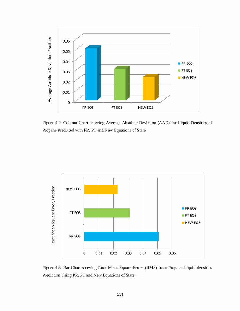
111
Figure 4.2: Column Chart showing Average Absolute Deviation (AAD) for Liquid Densities of
Propane Predicted with PR, PT and New Equations of State.
Figure 4.3: Bar Chart showing Root Mean Square Errors (RMS) from Propane Liquid densities
Prediction Using PR, PT and New Equations of State.
0
0.01
0.02
0.03
0.04
0.05
0.06
PR EOS PT EOS NEW EOS
PR EOS
PT EOS
NEW EOS
0 0.01 0.02 0.03 0.04 0.05 0.06
PR EOS
PT EOS
NEW EOS
PR EOS
PT EOS
NEW EOS
Ro
ot
Mea
n S
qu
are
Erro
r, F
ract
ion
A
vera
ge A
bso
lute
Dev
iati
on
, Fra
ctio
n

112
4.1c Iso-Butane
For the liquid density prediction of iso-butane, the fluid temperatures ranged from
40.0𝑜𝐹 𝑡𝑜 130.0𝑜𝐹 and pressures ranged from 27.0 𝑡𝑜 110.0 𝑝𝑠𝑖𝑎. The predicted and
experimental liquid densities over these temperature and pressure ranges are as shown in the
table below:
TABLE 4.1c(i) Calculated and Experimental Liquid Density of Iso-Butane:
Temperature
(oF)
Pressure
(Psia)
Experimental
𝜌 (𝑙𝑏 𝑓𝑡3⁄ )
PR-EOS
𝜌 (𝑙𝑏 𝑓𝑡3⁄ )
PT-EOS
𝜌 (𝑙𝑏 𝑓𝑡3⁄ )
NEW-EOS
𝜌 (𝑙𝑏 𝑓𝑡3⁄ )
40.0 27.0 35.9112 33.8447 36.6524 36.1064
60.0 38.0 35.11248 32.8196 35.7135 35.2102
80.0 52.5 34.23888 31.7305 34.7013 34.2526
100.0 71.5 33.34032 30.5702 33.6070 33.2264
130.0 110.0 31.83024 28.6689 31.7832 31.5366
Over these ranges of temperatures and pressures, the Peng-Robinson’s equation of state
gave an average absolute deviation (AAD) of 8.23% and a root mean square (RMS) error of
8.39%. patel and Teja’s predictions were better than those by Peng Robinson with average
absolute deviation of 1.19% and root mean square error of 1.36%. The AAD and RMS calculated
for the New equation of state are 0.004% and 0.005% respectively. These results are quite
impressive for showing minimal error when compared to Peng Robinson and Patel-Teja’s
predictions. The minimum absolute deviation was obtained as 4.01𝐸 − 04 and this was obtained
for predictions with the New equation of state. The maximum absolute deviation for these results
of table 4.1c(i) is 11.03% and this was obtained with the PR equation of state predictions. The
summary of errors from these values is as shown in the table below:
Table 4.1c(ii) Error Analysis for Liquid Densities Prediction for Iso-Butane
EOS AAD RMS
PR
PT
NEW
0.0823
0.0119
0.0043
0.0839
0.0137
0.0052
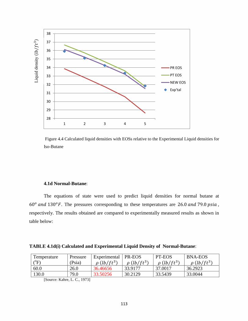
113
Figure 4.4 Calculated liquid densities with EOSs relative to the Experimental Liquid densities for
Iso-Butane
4.1d Normal-Butane:
The equations of state were used to predict liquid densities for normal butane at
60𝑜 𝑎𝑛𝑑 130𝑜𝐹. The pressures corresponding to these temperatures are 26.0 𝑎𝑛𝑑 79.0 𝑝𝑠𝑖𝑎 ,
respectively. The results obtained are compared to experimentally measured results as shown in
table below:
TABLE 4.1d(i) Calculated and Experimental Liquid Density of Normal-Butane:
Temperature
(oF)
Pressure
(Psia)
Experimental
𝜌 (𝑙𝑏 𝑓𝑡3⁄ )
PR-EOS
𝜌 (𝑙𝑏 𝑓𝑡3⁄ )
PT-EOS
𝜌 (𝑙𝑏 𝑓𝑡3⁄ )
BNA-EOS
𝜌 (𝑙𝑏 𝑓𝑡3⁄ )
60.0 26.0 36.46656 33.9177 37.0017 36.2923
130.0 79.0 33.50256 30.2129 33.5439 33.0044 [Source: Kahre, L. C., 1973]
28
29
30
31
32
33
34
35
36
37
38
1 2 3 4 5
PR EOS
PT EOS
NEW EOS
Exp'tal
Liq
uid
den
sity
(𝑙𝑏
𝑓𝑡3
⁄)

114
Analyzing the error from the predictions from the various equations of state reveals that
the average absolute deviations for PR, PT and New equations of state are, respectively, 9.20%,
0.79% and 0.995%. The root mean square error, (RMS) is for PR EOS, 9.36%, for PT EOS,
1.03% and for New EOS, 1.12%. The error is seen at a glance in the table below:
Table 4.1d(ii) Error Analysis for Liquid Densities Prediction for n-Butane
EOS AAD RMS
PR
PT
NEW
0.09202
0.00787
0.00995
0.0936
0.0103
0.0112
All the results of tables 4.1(a) through 4.1(d) are summarized in table 4.1(e) below. These
summarized result of error analyzed for all the single component systems considered reveals that
the New equation of state has the smallest average absolute error (1.75% ) and smallest root
mean square error (2.38%). The Peng Robinson equation of state had the highest average
absolute error of 38.82% and highest root mean square error of 86.33%. The extremely high
error values measured for the Peng-Robinson’s equation of state are due to the effect of the near
critical point predictions for which the Peng Robinson’s equation shows immense weakness. The
AAD and RMS are 4.99% and 8.15% for the Patel-Teja’s equation of state. Plots of the errors
(AAD and RMS) are shown for comparison of equations of state performances.
TABLE 4.1e: Summarized Results for Liquid Densities Prediction for All Single
Component Hydrocarbon Systems Considered
EOS 𝐍𝐃𝐏∗ AAD RMS
PR
PT
NEW
17
17
17
0.3882
0.0499
0.0175
0.8633
0.0815
0.0238
NDP∗ ≡ Number of Data Points

115
Figure 4.5 Bar Chart Representation of Root Mean Square Errors (RMS) for Liquid Density Predictions
Using: PR, PT and NEW EOSs for all Single Component Systems Analyzed
Figure 4.6: Column Chart showing Average Absolute Deviation (AAD) for PR, PT and New Equations of
State for all Single Component Systems Analyzed.
0 0.2 0.4 0.6 0.8 1
PR EOS
PT EOS
NEW EOS
PR EOS
PT EOS
NEW EOS
0
0.1
0.2
0.3
0.4
0.5
0.6
0.7
0.8
0.9
PR EOS PT EOS NEW EOS
PR EOS
PT EOS
NEW EOS
Ave
rage
Ab
solu
te D
evia
tio
n, F
ract
ion
Ro
ot
Mea
n s
qu
are
Erro
r, F
ract
ion
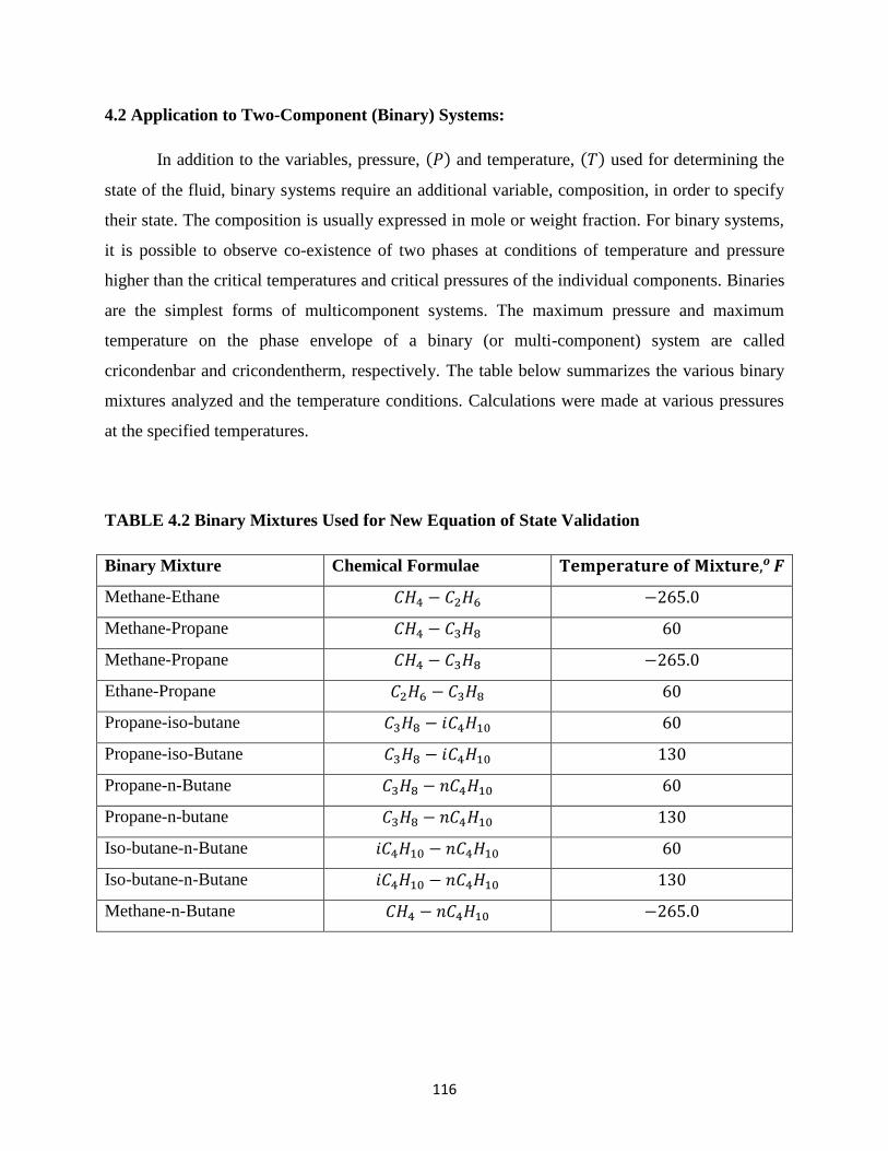
116
4.2 Application to Two-Component (Binary) Systems:
In addition to the variables, pressure, (𝑃) and temperature, (𝑇) used for determining the
state of the fluid, binary systems require an additional variable, composition, in order to specify
their state. The composition is usually expressed in mole or weight fraction. For binary systems,
it is possible to observe co-existence of two phases at conditions of temperature and pressure
higher than the critical temperatures and critical pressures of the individual components. Binaries
are the simplest forms of multicomponent systems. The maximum pressure and maximum
temperature on the phase envelope of a binary (or multi-component) system are called
cricondenbar and cricondentherm, respectively. The table below summarizes the various binary
mixtures analyzed and the temperature conditions. Calculations were made at various pressures
at the specified temperatures.
TABLE 4.2 Binary Mixtures Used for New Equation of State Validation
Binary Mixture Chemical Formulae 𝐓𝐞𝐦𝐩𝐞𝐫𝐚𝐭𝐮𝐫𝐞 𝐨𝐟 𝐌𝐢𝐱𝐭𝐮𝐫𝐞,𝒐 𝑭
Methane-Ethane 𝐶𝐻4 − 𝐶2𝐻6 −265.0
Methane-Propane 𝐶𝐻4 − 𝐶3𝐻8 60
Methane-Propane 𝐶𝐻4 − 𝐶3𝐻8 −265.0
Ethane-Propane 𝐶2𝐻6 − 𝐶3𝐻8 60
Propane-iso-butane 𝐶3𝐻8 − 𝑖𝐶4𝐻10 60
Propane-iso-Butane 𝐶3𝐻8 − 𝑖𝐶4𝐻10 130
Propane-n-Butane 𝐶3𝐻8 − 𝑛𝐶4𝐻10 60
Propane-n-butane 𝐶3𝐻8 − 𝑛𝐶4𝐻10 130
Iso-butane-n-Butane 𝑖𝐶4𝐻10 − 𝑛𝐶4𝐻10 60
Iso-butane-n-Butane 𝑖𝐶4𝐻10 − 𝑛𝐶4𝐻10 130
Methane-n-Butane 𝐶𝐻4 − 𝑛𝐶4𝐻10 −265.0
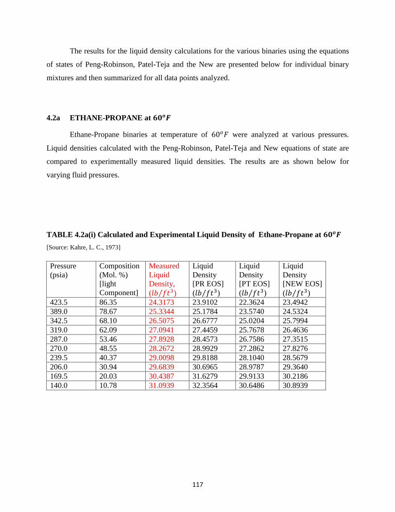
117
The results for the liquid density calculations for the various binaries using the equations
of states of Peng-Robinson, Patel-Teja and the New are presented below for individual binary
mixtures and then summarized for all data points analyzed.
4.2a ETHANE-PROPANE at 𝟔𝟎𝒐𝑭
Ethane-Propane binaries at temperature of 60𝑜𝐹 were analyzed at various pressures.
Liquid densities calculated with the Peng-Robinson, Patel-Teja and New equations of state are
compared to experimentally measured liquid densities. The results are as shown below for
varying fluid pressures.
TABLE 4.2a(i) Calculated and Experimental Liquid Density of Ethane-Propane at 𝟔𝟎𝒐𝑭
[Source: Kahre, L. C., 1973]
Pressure
(psia)
Composition
(Mol. %)
[light
Component]
Measured
Liquid
Density,
(𝑙𝑏 𝑓𝑡3⁄ )
Liquid
Density
[PR EOS]
(𝑙𝑏 𝑓𝑡3⁄ )
Liquid
Density
[PT EOS]
(𝑙𝑏 𝑓𝑡3⁄ )
Liquid
Density
[NEW EOS]
(𝑙𝑏 𝑓𝑡3⁄ )
423.5 86.35 24.3173 23.9102 22.3624 23.4942
389.0 78.67 25.3344 25.1784 23.5740 24.5324
342.5 68.10 26.5075 26.6777 25.0204 25.7994
319.0 62.09 27.0941 27.4459 25.7678 26.4636
287.0 53.46 27.8928 28.4573 26.7586 27.3515
270.0 48.55 28.2672 28.9929 27.2862 27.8276
239.5 40.37 29.0098 29.8188 28.1040 28.5679
206.0 30.94 29.6839 30.6965 28.9787 29.3640
169.5 20.03 30.4387 31.6279 29.9133 30.2186
140.0 10.78 31.0939 32.3564 30.6486 30.8939
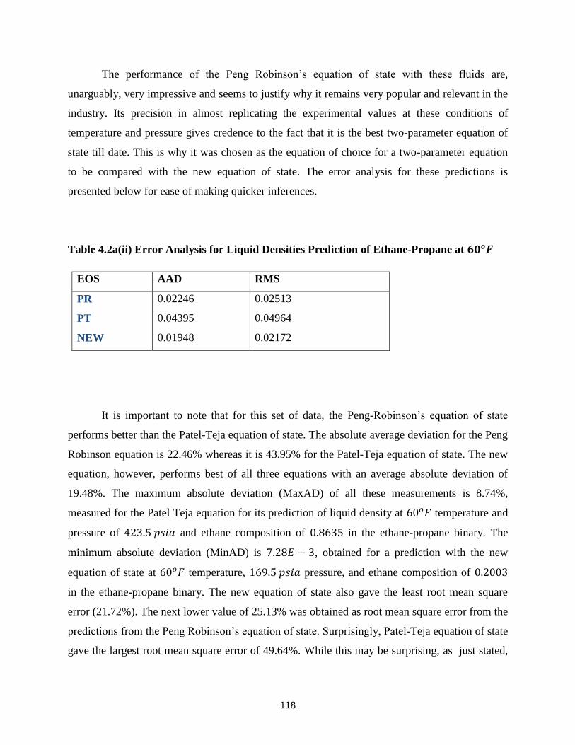
118
The performance of the Peng Robinson’s equation of state with these fluids are,
unarguably, very impressive and seems to justify why it remains very popular and relevant in the
industry. Its precision in almost replicating the experimental values at these conditions of
temperature and pressure gives credence to the fact that it is the best two-parameter equation of
state till date. This is why it was chosen as the equation of choice for a two-parameter equation
to be compared with the new equation of state. The error analysis for these predictions is
presented below for ease of making quicker inferences.
Table 4.2a(ii) Error Analysis for Liquid Densities Prediction of Ethane-Propane at 𝟔𝟎𝒐𝑭
EOS AAD RMS
PR
PT
NEW
0.02246
0.04395
0.01948
0.02513
0.04964
0.02172
It is important to note that for this set of data, the Peng-Robinson’s equation of state
performs better than the Patel-Teja equation of state. The absolute average deviation for the Peng
Robinson equation is 22.46% whereas it is 43.95% for the Patel-Teja equation of state. The new
equation, however, performs best of all three equations with an average absolute deviation of
19.48%. The maximum absolute deviation (MaxAD) of all these measurements is 8.74%,
measured for the Patel Teja equation for its prediction of liquid density at 60𝑜𝐹 temperature and
pressure of 423.5 𝑝𝑠𝑖𝑎 and ethane composition of 0.8635 in the ethane-propane binary. The
minimum absolute deviation (MinAD) is 7.28𝐸 − 3, obtained for a prediction with the new
equation of state at 60𝑜𝐹 temperature, 169.5 𝑝𝑠𝑖𝑎 pressure, and ethane composition of 0.2003
in the ethane-propane binary. The new equation of state also gave the least root mean square
error (21.72%). The next lower value of 25.13% was obtained as root mean square error from the
predictions from the Peng Robinson’s equation of state. Surprisingly, Patel-Teja equation of state
gave the largest root mean square error of 49.64%. While this may be surprising, as just stated,

119
the average overall performance of the Peng-Robinson’s equation for a large data set of various
binaries at different thermodynamic conditions do not always follow this trend.
The relative positioning of these predictions from the various equations of state relative
to the experimental results could be viewed at a glance from figure 4.7 below:
Figure 4.7 Relative Positions of liquid densities predicted by PR EOS, PT EOS and New EOS relative to
Experimental density trend.
It can be deduced from the plot of figure 4.7 that, at higher molar composition of the light
hydrocarbon fraction (Ethane), the PR EOS better predicts its liquid densities whereas at lower
light hydrocarbon fraction composition, the New equation of state predicts its liquid densities
better at various pressures. Also at low light hydrocarbon fraction composition (high ethane
fraction), the Patel-Teja’s equation of state predictions improve over that of Peng-Robinson’s
equation of state predictions.
22
24
26
28
30
32
1 2 3 4 5 6 7 8 9 10
PR EOS
PT EOS
NEW EOS
EXPTAL
Liq
uid
Den
siti
es in
𝑙𝑏
𝑓𝑡3
⁄

120
4.2b Propane-Isobutane at 𝟔𝟎𝒐𝑭
The liquid densities of binary mixtures of propane- isobutane (𝐶3𝐻8 − 𝑖 − 𝐶4𝐻10) at varying
pressures and at a temperature of 60𝑜𝐹, were calculated using the Peng-Robinson’s, Patel-
Teja’s and New equations of state. The calculated and experimentally derived results are as
shown below:
TABLE 4.2b(i) Calculated and Experimental Liquid Density of Propane-Iso-Butane at
𝟔𝟎𝒐𝑭
Pressure
(psia)
Composition
(Mol. %)
[light
Component]
Measured
Liquid
Density,
(𝑙𝑏 𝑓𝑡3⁄ )
Liquid
Density
[PR EOS]
(𝑙𝑏 𝑓𝑡3⁄ )
Liquid
Density
[PT EOS]
(𝑙𝑏 𝑓𝑡3⁄ )
Liquid
Density
[NEW EOS]
(𝑙𝑏 𝑓𝑡3⁄ )
96.0 84.64 32.29824 33.8922 32.2291 32.3041
85.0 70.38 32.86608 34.5367 32.9055 32.8917
70.0 49.32 33.61488 35.4153 33.8314 33.7037
57.5 30.21 34.2264 36.1456 34.6051 34.3885
47.5 14.15 34.70688 36.7159 35.2114 34.9290
The average absolute deviations of the predictions with Peng-Robinson’s, Patel-Teja’s
and the New equations of state are 5.08%, 0.70% and 0.29%, respectively. The improvement by
the New equation is quite significant, reducing the error by more than fifty percent. The root
mean square error from the predictions with PR EOS is 5.09%. The root mean square error due
to predictions with the Patel-Teja equation is 0.863%, an improvement over the Peng Robinson’s
effort. The New equation gave a root mean square error of 3.75%, the least recorded. The errors
due to these predictions are as summarized in the table below:
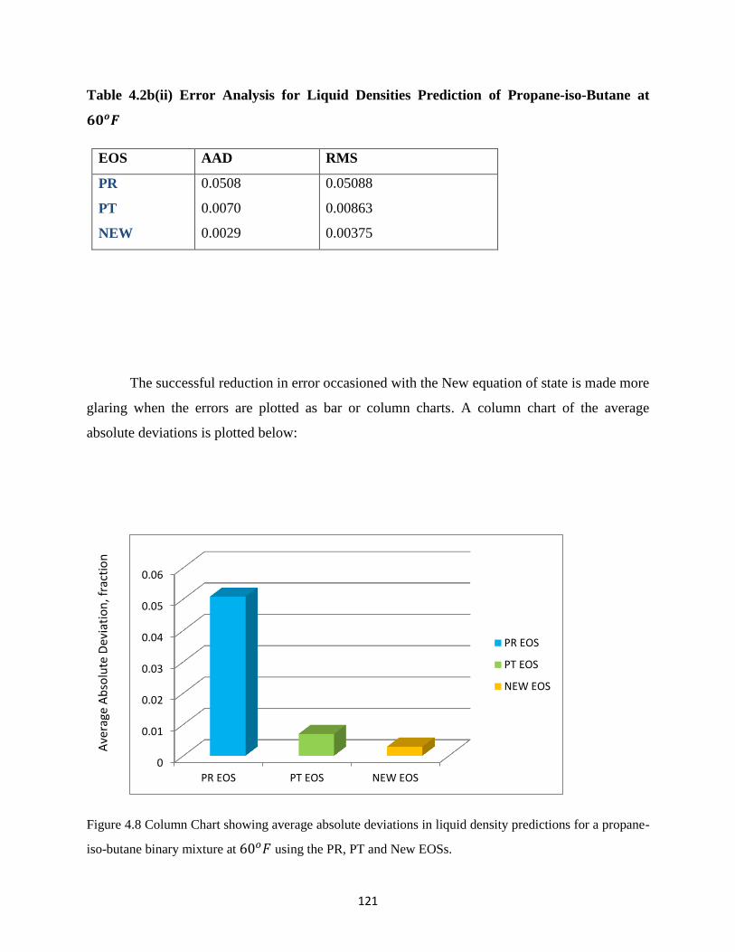
121
Table 4.2b(ii) Error Analysis for Liquid Densities Prediction of Propane-iso-Butane at
𝟔𝟎𝒐𝑭
EOS AAD RMS
PR
PT
NEW
0.0508
0.0070
0.0029
0.05088
0.00863
0.00375
The successful reduction in error occasioned with the New equation of state is made more
glaring when the errors are plotted as bar or column charts. A column chart of the average
absolute deviations is plotted below:
Figure 4.8 Column Chart showing average absolute deviations in liquid density predictions for a propane-
iso-butane binary mixture at 60𝑜𝐹 using the PR, PT and New EOSs.
0
0.01
0.02
0.03
0.04
0.05
0.06
PR EOS PT EOS NEW EOS
PR EOS
PT EOS
NEW EOS
Ave
rage
Ab
solu
te D
evia
tio
n, f
ract
ion
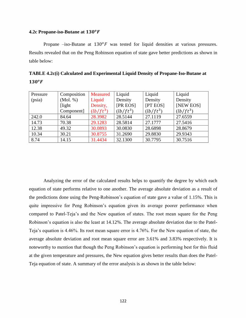
122
4.2c Propane-iso-Butane at 𝟏𝟑𝟎𝒐𝑭
Propane –iso-Butane at 130𝑜𝐹 was tested for liquid densities at various pressures.
Results revealed that on the Peng Robinson equation of state gave better predictions as shown in
table below:
TABLE 4.2c(i) Calculated and Experimental Liquid Density of Propane-Iso-Butane at
𝟏𝟑𝟎𝒐𝑭
Pressure
(psia)
Composition
(Mol. %)
[light
Component]
Measured
Liquid
Density,
(𝑙𝑏 𝑓𝑡3⁄ )
Liquid
Density
[PR EOS]
(𝑙𝑏 𝑓𝑡3⁄ )
Liquid
Density
[PT EOS]
(𝑙𝑏 𝑓𝑡3⁄ )
Liquid
Density
[NEW EOS]
(𝑙𝑏 𝑓𝑡3⁄ )
242.0 84.64 28.3982 28.5144 27.1119 27.6559
14.73 70.38 29.1283 28.5814 27.1777 27.5416
12.38 49.32 30.0893 30.0830 28.6898 28.8679
10.34 30.21 30.8755 31.2690 29.8830 29.9343
8.74 14.15 31.4434 32.1300 30.7795 30.7516
Analyzing the error of the calculated results helps to quantify the degree by which each
equation of state performs relative to one another. The average absolute deviation as a result of
the predictions done using the Peng-Robinson’s equation of state gave a value of 1.15%. This is
quite impressive for Peng Robinson’s equation given its average poorer performance when
compared to Patel-Teja’s and the New equation of states. The root mean square for the Peng
Robinson’s equation is also the least at 14.12%. The average absolute deviation due to the Patel-
Teja’s equation is 4.46%. Its root mean square error is 4.76%. For the New equation of state, the
average absolute deviation and root mean square error are 3.61% and 3.83% respectively. It is
noteworthy to mention that though the Peng Robinson’s equation is performing best for this fluid
at the given temperature and pressures, the New equation gives better results than does the Patel-
Teja equation of state. A summary of the error analysis is as shown in the table below:
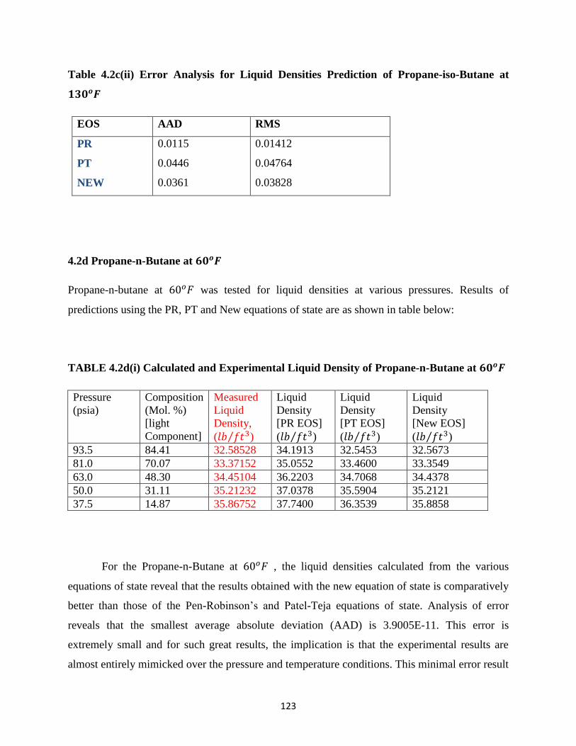
123
Table 4.2c(ii) Error Analysis for Liquid Densities Prediction of Propane-iso-Butane at
𝟏𝟑𝟎𝒐𝑭
EOS AAD RMS
PR
PT
NEW
0.0115
0.0446
0.0361
0.01412
0.04764
0.03828
4.2d Propane-n-Butane at 𝟔𝟎𝒐𝑭
Propane-n-butane at 60𝑜𝐹 was tested for liquid densities at various pressures. Results of
predictions using the PR, PT and New equations of state are as shown in table below:
TABLE 4.2d(i) Calculated and Experimental Liquid Density of Propane-n-Butane at 𝟔𝟎𝒐𝑭
Pressure
(psia)
Composition
(Mol. %)
[light
Component]
Measured
Liquid
Density,
(𝑙𝑏 𝑓𝑡3⁄ )
Liquid
Density
[PR EOS]
(𝑙𝑏 𝑓𝑡3⁄ )
Liquid
Density
[PT EOS]
(𝑙𝑏 𝑓𝑡3⁄ )
Liquid
Density
[New EOS]
(𝑙𝑏 𝑓𝑡3⁄ )
93.5 84.41 32.58528 34.1913 32.5453 32.5673
81.0 70.07 33.37152 35.0552 33.4600 33.3549
63.0 48.30 34.45104 36.2203 34.7068 34.4378
50.0 31.11 35.21232 37.0378 35.5904 35.2121
37.5 14.87 35.86752 37.7400 36.3539 35.8858
For the Propane-n-Butane at 60𝑜𝐹 , the liquid densities calculated from the various
equations of state reveal that the results obtained with the new equation of state is comparatively
better than those of the Pen-Robinson’s and Patel-Teja equations of state. Analysis of error
reveals that the smallest average absolute deviation (AAD) is 3.9005E-11. This error is
extremely small and for such great results, the implication is that the experimental results are
almost entirely mimicked over the pressure and temperature conditions. This minimal error result
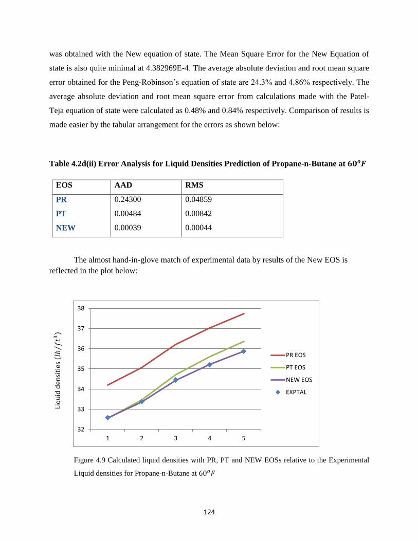
124
was obtained with the New equation of state. The Mean Square Error for the New Equation of
state is also quite minimal at 4.382969E-4. The average absolute deviation and root mean square
error obtained for the Peng-Robinson’s equation of state are 24.3% and 4.86% respectively. The
average absolute deviation and root mean square error from calculations made with the Patel-
Teja equation of state were calculated as 0.48% and 0.84% respectively. Comparison of results is
made easier by the tabular arrangement for the errors as shown below:
Table 4.2d(ii) Error Analysis for Liquid Densities Prediction of Propane-n-Butane at 𝟔𝟎𝒐𝑭
EOS AAD RMS
PR
PT
NEW
0.24300
0.00484
0.00039
0.04859
0.00842
0.00044
The almost hand-in-glove match of experimental data by results of the New EOS is
reflected in the plot below:
Figure 4.9 Calculated liquid densities with PR, PT and NEW EOSs relative to the Experimental
Liquid densities for Propane-n-Butane at 60𝑜𝐹
32
33
34
35
36
37
38
1 2 3 4 5
PR EOS
PT EOS
NEW EOS
EXPTAL
Liq
uid
den
siti
es (
𝑙𝑏𝑓
𝑡3⁄
)

125
4.2e Propane-n-Butane at 𝟏𝟑𝟎𝒐𝑭
The binary fluid, Propane-n-butane was subjected to various pressures at 130𝑜𝐹 and its liquid
densities at these conditions measured. The experimental results, obtained in literature, were
compared with results calculated using the Peng Robinson’s, Patel-Teja’s and New equations of
state. The results obtained are as tabulated below:
TABLE 4.2e(i) Calculated and Experimental Liquid Density of Propane-n-Butane at
𝟏𝟑𝟎𝒐𝑭
Pressure (psia) Composition
(Mol. %)
[light
Component]
Measured
Liquid
Density,
(𝑙𝑏 𝑓𝑡3⁄ )
Liquid
Density
[PR EOS]
(𝑙𝑏 𝑓𝑡3⁄ )
Liquid
Density
[PT EOS]
(𝑙𝑏 𝑓𝑡3⁄ )
Liquid
Density
[NEW EOS]
(𝑙𝑏 𝑓𝑡3⁄ )
236.0 84.41 28.7726 29.0071 27.6028 28.0569
205.0 70.07 29.7960 30.2739 28.8804 29.1342
163.0 48.30 31.1376 31.9231 30.5668 30.5788
131.0 31.11 32.0736 33.0424 31.7263 31.5836
103.5 14.87 32.8411 33.9890 32.7161 32.4489
A quick and general look at the results in the table reveals that the new equation of state
is giving better predictions than do the Peng-Robinson’s and Patel-Teja’s equations of state. By
statistically analyzing the above data, a more conclusive inference can be drawn on the
performance patterns of the various equations of state. The results of analyzing the error due to
the predictions by these various equations of state are as tabulated below:
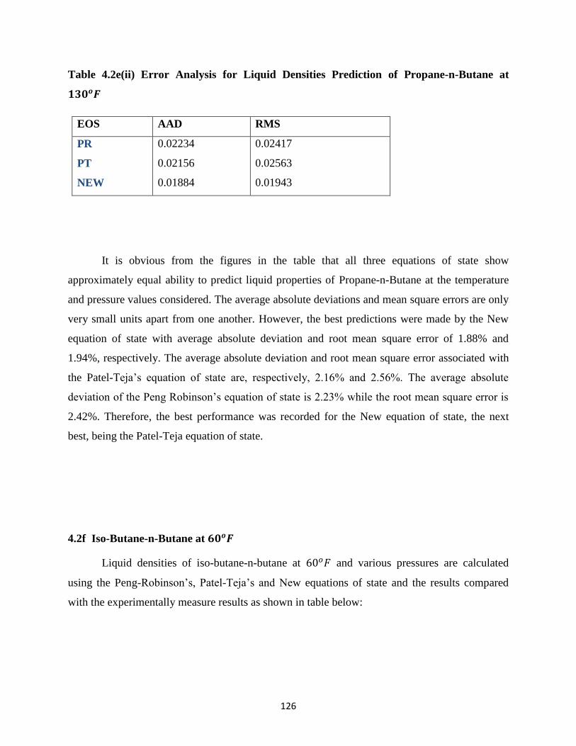
126
Table 4.2e(ii) Error Analysis for Liquid Densities Prediction of Propane-n-Butane at
𝟏𝟑𝟎𝒐𝑭
EOS AAD RMS
PR
PT
NEW
0.02234
0.02156
0.01884
0.02417
0.02563
0.01943
It is obvious from the figures in the table that all three equations of state show
approximately equal ability to predict liquid properties of Propane-n-Butane at the temperature
and pressure values considered. The average absolute deviations and mean square errors are only
very small units apart from one another. However, the best predictions were made by the New
equation of state with average absolute deviation and root mean square error of 1.88% and
1.94%, respectively. The average absolute deviation and root mean square error associated with
the Patel-Teja’s equation of state are, respectively, 2.16% and 2.56%. The average absolute
deviation of the Peng Robinson’s equation of state is 2.23% while the root mean square error is
2.42%. Therefore, the best performance was recorded for the New equation of state, the next
best, being the Patel-Teja equation of state.
4.2f Iso-Butane-n-Butane at 𝟔𝟎𝒐𝑭
Liquid densities of iso-butane-n-butane at 60𝑜𝐹 and various pressures are calculated
using the Peng-Robinson’s, Patel-Teja’s and New equations of state and the results compared
with the experimentally measure results as shown in table below:
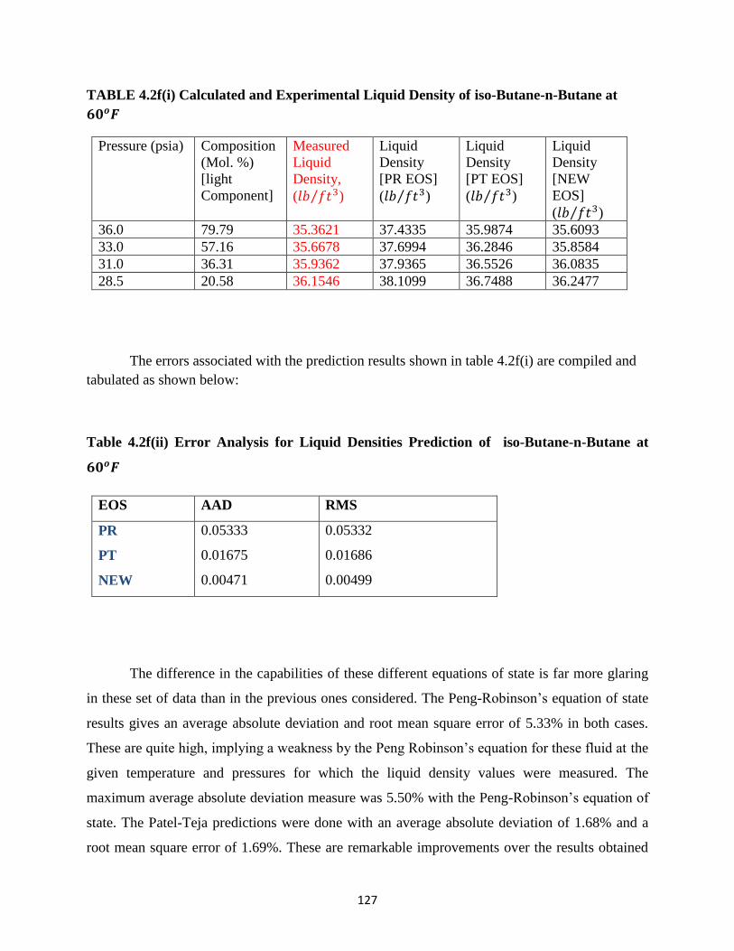
127
TABLE 4.2f(i) Calculated and Experimental Liquid Density of iso-Butane-n-Butane at
𝟔𝟎𝒐𝑭
Pressure (psia) Composition
(Mol. %)
[light
Component]
Measured
Liquid
Density,
(𝑙𝑏 𝑓𝑡3⁄ )
Liquid
Density
[PR EOS]
(𝑙𝑏 𝑓𝑡3⁄ )
Liquid
Density
[PT EOS]
(𝑙𝑏 𝑓𝑡3⁄ )
Liquid
Density
[NEW
EOS]
(𝑙𝑏 𝑓𝑡3⁄ )
36.0 79.79 35.3621 37.4335 35.9874 35.6093
33.0 57.16 35.6678 37.6994 36.2846 35.8584
31.0 36.31 35.9362 37.9365 36.5526 36.0835
28.5 20.58 36.1546 38.1099 36.7488 36.2477
The errors associated with the prediction results shown in table 4.2f(i) are compiled and
tabulated as shown below:
Table 4.2f(ii) Error Analysis for Liquid Densities Prediction of iso-Butane-n-Butane at
𝟔𝟎𝒐𝑭
EOS AAD RMS
PR
PT
NEW
0.05333
0.01675
0.00471
0.05332
0.01686
0.00499
The difference in the capabilities of these different equations of state is far more glaring
in these set of data than in the previous ones considered. The Peng-Robinson’s equation of state
results gives an average absolute deviation and root mean square error of 5.33% in both cases.
These are quite high, implying a weakness by the Peng Robinson’s equation for these fluid at the
given temperature and pressures for which the liquid density values were measured. The
maximum average absolute deviation measure was 5.50% with the Peng-Robinson’s equation of
state. The Patel-Teja predictions were done with an average absolute deviation of 1.68% and a
root mean square error of 1.69%. These are remarkable improvements over the results obtained
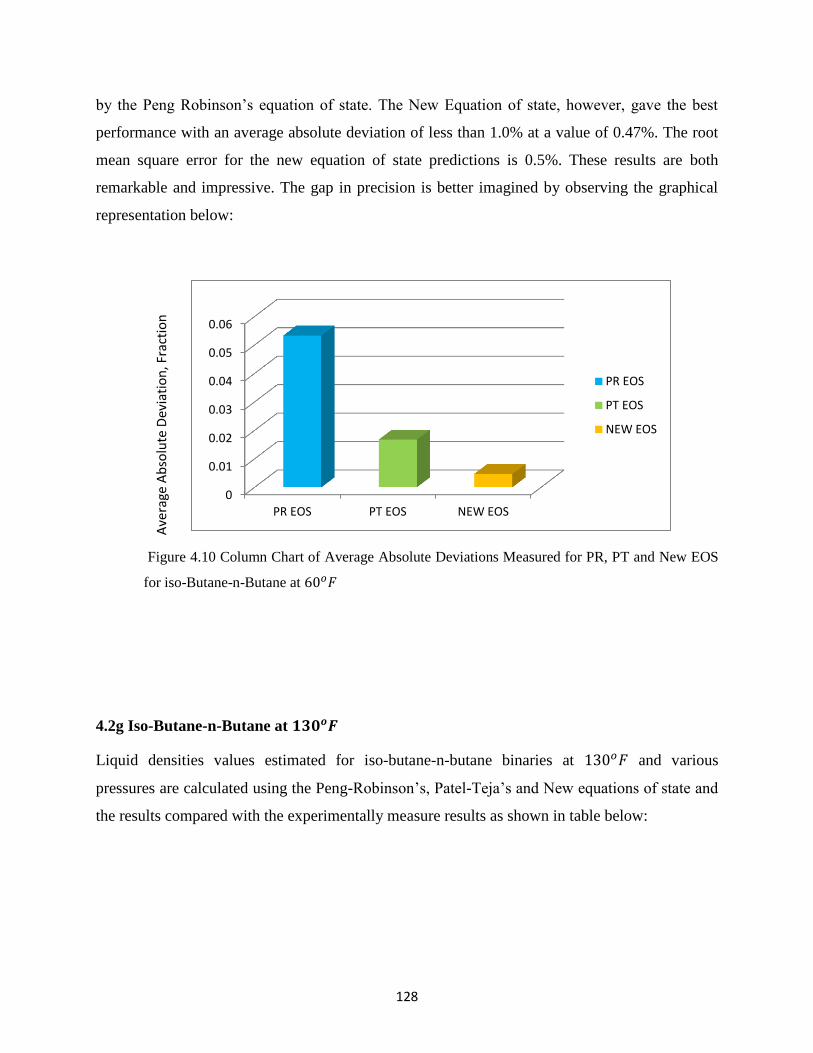
128
by the Peng Robinson’s equation of state. The New Equation of state, however, gave the best
performance with an average absolute deviation of less than 1.0% at a value of 0.47%. The root
mean square error for the new equation of state predictions is 0.5%. These results are both
remarkable and impressive. The gap in precision is better imagined by observing the graphical
representation below:
Figure 4.10 Column Chart of Average Absolute Deviations Measured for PR, PT and New EOS
for iso-Butane-n-Butane at 60𝑜𝐹
4.2g Iso-Butane-n-Butane at 𝟏𝟑𝟎𝒐𝑭
Liquid densities values estimated for iso-butane-n-butane binaries at 130𝑜𝐹 and various
pressures are calculated using the Peng-Robinson’s, Patel-Teja’s and New equations of state and
the results compared with the experimentally measure results as shown in table below:
0
0.01
0.02
0.03
0.04
0.05
0.06
PR EOS PT EOS NEW EOS
PR EOS
PT EOS
NEW EOS
Ave
rage
Ab
solu
te D
evia
tio
n, F
ract
ion
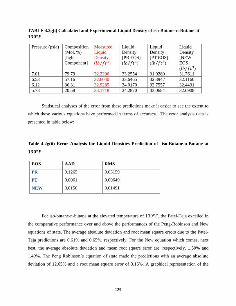
129
TABLE 4.2g(i) Calculated and Experimental Liquid Density of iso-Butane-n-Butane at
𝟏𝟑𝟎𝒐𝑭
Pressure (psia) Composition
(Mol. %)
[light
Component]
Measured
Liquid
Density,
(𝑙𝑏 𝑓𝑡3⁄ )
Liquid
Density
[PR EOS]
(𝑙𝑏 𝑓𝑡3⁄ )
Liquid
Density
[PT EOS]
(𝑙𝑏 𝑓𝑡3⁄ )
Liquid
Density
[NEW
EOS]
(𝑙𝑏 𝑓𝑡3⁄ )
7.01 79.79 32.2296 33.2554 31.9280 31.7611
6.53 57.16 32.6040 33.6465 32.3947 32.1160
6.12 36.31 32.9285 34.0170 32.7557 32.4431
5.78 20.58 33.1718 34.2870 33.0684 32.6908
Statistical analyses of the error from these predictions make it easier to see the extent to
which these various equations have performed in terms of accuracy. The error analysis data is
presented in table below:
Table 4.2g(ii) Error Analysis for Liquid Densities Prediction of iso-Butane-n-Butane at
𝟏𝟑𝟎𝒐𝑭
EOS AAD RMS
PR
PT
NEW
0.1265
0.0061
0.0150
0.03159
0.00649
0.01491
For iso-butane-n-butane at the elevated temperature of 130𝑜𝐹, the Patel-Teja excelled in
the comparative performance over and above the performances of the Peng-Robinson and New
equations of state. The average absolute deviation and root mean square errors due to the Patel-
Teja predictions are 0.61% and 0.65%, respectively. For the New equation which comes, next
best, the average absolute deviation and mean root square error are, respectively, 1.50% and
1.49%. The Peng Robinson’s equation of state made the predictions with an average absolute
deviation of 12.65% and a root mean square error of 3.16%. A graphical representation of the

130
root mean square errors from the liquid density predictions with PR, PT and New EOS of iso-
butane-n-butane binaries at 130𝑜𝐹 is shown below with a bar chart.
Figure 4.11 Bar Chart of Root Mean square Errors Measured for PR, PT and New EOS for iso-
Butane-n-Butane at 130𝑜𝐹
4.2h Methane-Ethane at −𝟐𝟔𝟓. 𝟎𝒐𝑭
The next set of binary data considered, (4.2h through 4.2j) are taken from the work of
Shana’a and Canfield (1968). The liquid densities from experimental measurements are
compared with the results obtained from calculating the liquid densities of methane-ethane
0 0.005 0.01 0.015 0.02 0.025 0.03 0.035
PR EOS
PT EOS
NEW EOS
PR EOS
PT EOS
NEW EOS
Ro
ot
Mea
n S
qu
are
Erro
r (F
ract
ion
)

131
binaries at −265.0𝑜𝐹, and various pressures. The results obtained are tabulated in table 4.2h
below:
TABLE 4.2h(i) Calculated and Experimental Liquid Density of Methane-Ethane at
−𝟐𝟔𝟓. 𝟎𝒐𝑭
Pressure (psia) Composition
(Mol.)
[light
Component]
Measured
Liquid
Density,
(𝑙𝑏 𝑓𝑡3⁄ )
Liquid
Density
[PR EOS]
(𝑙𝑏 𝑓𝑡3⁄ )
Liquid
Density
[PT EOS]
(𝑙𝑏 𝑓𝑡3⁄ )
Liquid
Density
[NEW
EOS]
(𝑙𝑏 𝑓𝑡3⁄ )
2.9008 0.1902 37.6796 40.5714 37.8657 37.7558
4.6412 0.3426 36.0909 39.1313 36.3865 36.3028
6.0916 0.5454 33.7086 36.9067 34.1051 34.0651
7.8320 0.6767 31.9781 35.2454 32.4078 32.3955
9.4275 0.8668 29.0321 32.4036 29.5546 29.6003
11.0229 1.0000 26.6905 30.0164 27.1970 27.3025
The superior performance of the New equation of state for the temperature and pressure
values shown in Table 4.2h(i), is shown by the error analysis shown below:
Table 4.2h(ii) Error Analysis for Liquid Densities Prediction of Methane-Ethane at
−𝟐𝟔𝟓. 𝟎𝒐𝑭
EOS AAD RMS
PR
PT
NEW
0.0898
0.0125
0.0121
0.09177
0.01330
0.01405
The average absolute deviations from the Peng-Robinson’s equation of state calculations
are the highest with a value of 8.98%. The root mean square error from the Peng Robinson’s
equation is 9.18%. The best estimated values of methane-ethane liquid densities at -265 degree
Fahrenheit temperature and various pressures was obtained with an average absolute deviation of
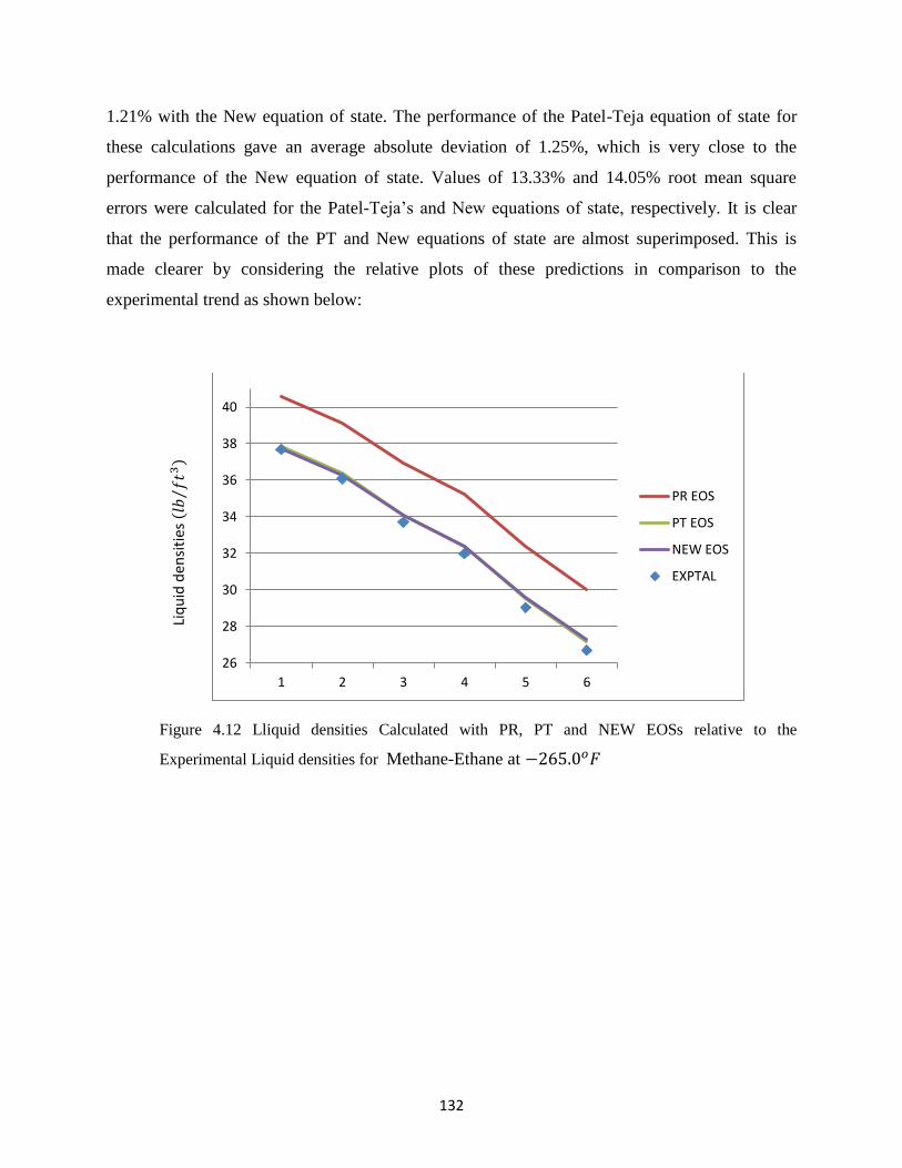
132
1.21% with the New equation of state. The performance of the Patel-Teja equation of state for
these calculations gave an average absolute deviation of 1.25%, which is very close to the
performance of the New equation of state. Values of 13.33% and 14.05% root mean square
errors were calculated for the Patel-Teja’s and New equations of state, respectively. It is clear
that the performance of the PT and New equations of state are almost superimposed. This is
made clearer by considering the relative plots of these predictions in comparison to the
experimental trend as shown below:
Figure 4.12 Lliquid densities Calculated with PR, PT and NEW EOSs relative to the
Experimental Liquid densities for Methane-Ethane at −265.0𝑜𝐹
26
28
30
32
34
36
38
40
1 2 3 4 5 6
PR EOS
PT EOS
NEW EOS
EXPTAL
Liq
uid
den
siti
es (
𝑙𝑏𝑓
𝑡3⁄
)

133
4.2i Methane-Propane at −𝟐𝟔𝟓. 𝟎𝒐𝑭
The prediction results using the various equations to calculate the liquid densities of
methane-propane binaries at -265.0 degree Fahrenheit temperature are as tabulated below:
TABLE 4.2i(i) Calculated and Experimental Liquid Density of Methane-Propane at
−𝟐𝟔𝟓. 𝟎𝒐𝑭
Pressure (psia) Composition
(Mol.)
[light
Component]
Measured
Liquid
Density,
(𝑙𝑏 𝑓𝑡3⁄ )
Liquid
Density
[PR EOS]
(𝑙𝑏 𝑓𝑡3⁄ )
Liquid
Density
[PT EOS]
(𝑙𝑏 𝑓𝑡3⁄ )
Liquid
Density
[NEW EOS]
(𝑙𝑏 𝑓𝑡3⁄ )
4.6412 0.2575 41.6020 43.4996 41.2288 40.9971
6.0916 0.4068 39.6792 41.8954 39.4986 39.2952
7.5420 0.5504 37.4568 40.0090 37.4844 37.3195
8.7023 0.6924 34.7874 37.6902 35.0378 34.9283
10.0076 0.8484 31.1759 34.3916 31.6182 31.5918
Statistical error analysis of the results of table 4.2i(i) show that the Patel-Teja equation of
state gives better results for these set of data analyzed at the given temperature and pressures
considered. The minimum absolute deviation of 7.36E-04 was obtained with the Patel-Teja’s
equation of state. The Peng Robinson’s equation of state gave the maximum absolute deviation
of 6.4E-02 and an average absolute deviation of 6.64%. The root mean square error due to the
predictions of with the Peng Robinson’s equation of state is 6.85%. The average absolute
deviations of the Patel Teja and the New equations of state are, 0.71% and 0.91%, respectively.
The root mean square errors measured for these various equations are tabulated below.
Table 4.2i(ii) Error Analysis for Liquid Densities Prediction of Methane-Propane at
−𝟐𝟔𝟓. 𝟎𝒐𝑭
EOS AAD RMS
PR
PT
NEW
0.0664
0.0071
0.0091
0.06852
0.00837
0.01018

134
Though the Patel-Teja equation performs better than the New equation for these data set,
the difference is not significant as shown by the plot of liquid density profiles in comparison with
the experimentally derived liquid density profile.
Figure 4.13 Calculated liquid densities with PR, PT and NEW EOSs relative to the Experimental
Liquid densities for Methane-Propane at −265.0𝑜𝐹
4.2j Methane-n-Butane at −𝟐𝟔𝟓. 𝟎𝒐𝑭
Liquid densities for a binary mixture of methane-n-Butane at −265.00𝑜𝐹 temperature and
10.8778 psia pressure were calculated using the Peng Robinson’s, Patel-Teja’s and New
equations of state. The results obtained, shown below shows a narrow improvement by the New
equation over the Patel-Teja’s prediction. Results are shown in table below:
31
33
35
37
39
41
43
1 2 3 4 5
PR EOS
PT EOS
NEW EOS
EXPTAL
Liq
uid
den
sity
(𝑙𝑏
𝑓𝑡3
⁄)

135
TABLE 4.2j(i) Calculated and Experimental Liquid Density of Methane-n-Butane at
−𝟐𝟔𝟓. 𝟎𝒐𝑭
Pressure (psi) Composition
(Mol.)
[light
Component]
Measured
Liquid
Density
(𝑙𝑏 𝑓𝑡3⁄ )
Liquid
Density
[PR EOS]
(𝑙𝑏 𝑓𝑡3⁄ )
Liquid
Density
[PT EOS]
(𝑙𝑏 𝑓𝑡3⁄ )
Liquid
Density
[NEW EOS]
(𝑙𝑏 𝑓𝑡3⁄ )
10.8778 0.8843 31.5973 34.6560 31.9637 31.8905
The average absolute deviation for the predictions with PR, PT and New equations of
state are, 8.80%, 1.15% and 0.92% respectively, making the new equation a better predictor of
liquid density at the specified conditions of temperature and pressure.
The entire results for all the binary systems analyzed are summarized in the table below. The
lowest average absolute deviation for all the fifty data points considered was calculated for the
New equation of state as 1.60%. The next lowest value of 2.24% was obtained for the Patel-Teja
equation and the highest value of 4.53% was obtained for the Peng-Robinson’s equation of state.
TABLE 4.2k: Summary of Error Analysis for Liquid Density Prediction for All Binary
Hydrocarbon Mixtures Considered
EOS NDP AAD RMS
PR
PT
NEW
50
50
50
0.0453
0.0224
0.0160
0.0507
0.0310
0.0228
The results are better appreciated by observing the error margins on the column plot
below for first, the average absolute deviations and then the mean square errors obtained for the
various equations of state.
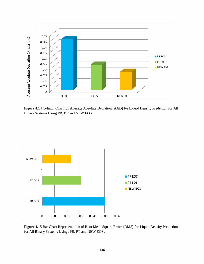
136
Figure 4.14 Column Chart for Average Absolute Deviation (AAD) for Liquid Density Prediction for All
Binary Systems Using PR, PT and NEW EOS.
Figure 4.15 Bar Chart Representation of Root Mean Square Errors (RMS) for Liquid Density Predictions
for All Binary Systems Using: PR, PT and NEW EOSs
0 0.01 0.02 0.03 0.04 0.05 0.06
PR EOS
PT EOS
NEW EOS
PR EOS
PT EOS
NEW EOS
Ave
rage
Ab
solu
te D
evia
tio
n (
𝐹𝑟𝑎
𝑐𝑡𝑖𝑜
𝑛)
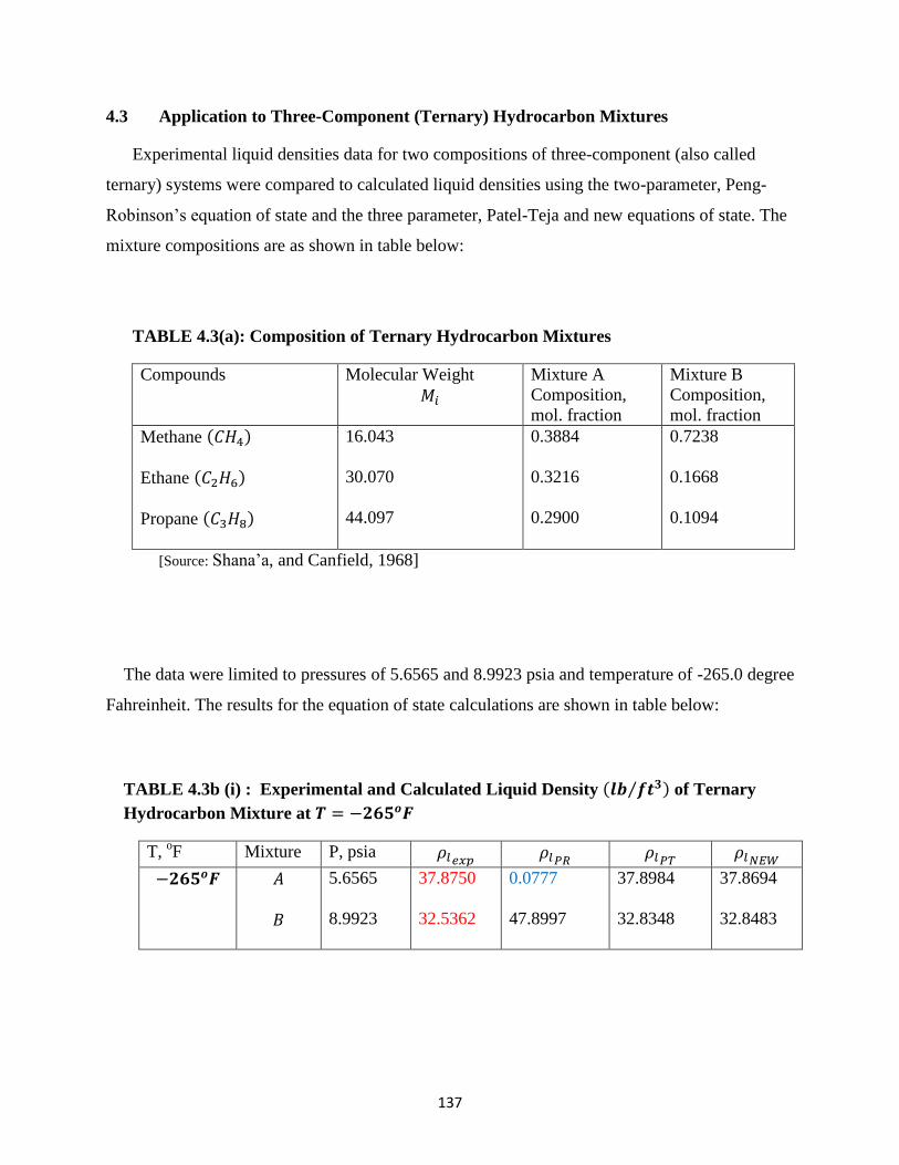
137
4.3 Application to Three-Component (Ternary) Hydrocarbon Mixtures
Experimental liquid densities data for two compositions of three-component (also called
ternary) systems were compared to calculated liquid densities using the two-parameter, Peng-
Robinson’s equation of state and the three parameter, Patel-Teja and new equations of state. The
mixture compositions are as shown in table below:
TABLE 4.3(a): Composition of Ternary Hydrocarbon Mixtures
Compounds Molecular Weight
𝑀𝑖
Mixture A
Composition,
mol. fraction
Mixture B
Composition,
mol. fraction
Methane (𝐶𝐻4)
Ethane (𝐶2𝐻6)
Propane (𝐶3𝐻8)
16.043
30.070
44.097
0.3884
0.3216
0.2900
0.7238
0.1668
0.1094
[Source: Shana’a, and Canfield, 1968]
The data were limited to pressures of 5.6565 and 8.9923 psia and temperature of -265.0 degree
Fahreinheit. The results for the equation of state calculations are shown in table below:
TABLE 4.3b (i) : Experimental and Calculated Liquid Density (𝒍𝒃 𝒇𝒕𝟑⁄ ) of Ternary
Hydrocarbon Mixture at 𝑻 = −𝟐𝟔𝟓𝒐𝑭
T, oF Mixture P, psia 𝜌𝑙𝑒𝑥𝑝
𝜌𝑙𝑃𝑅 𝜌𝑙𝑃𝑇
𝜌𝑙𝑁𝐸𝑊
−𝟐𝟔𝟓𝒐𝑭 𝐴
𝐵
5.6565
8.9923
37.8750
32.5362
0.0777
47.8997
37.8984
32.8348
37.8694
32.8483
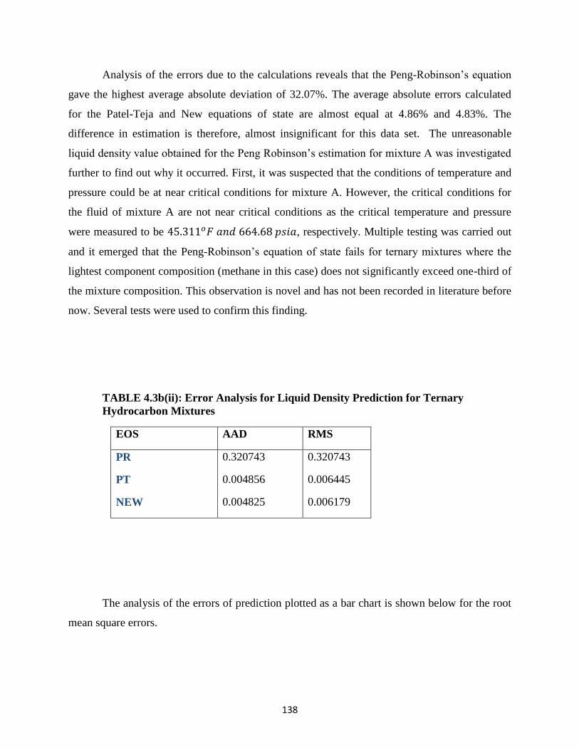
138
Analysis of the errors due to the calculations reveals that the Peng-Robinson’s equation
gave the highest average absolute deviation of 32.07%. The average absolute errors calculated
for the Patel-Teja and New equations of state are almost equal at 4.86% and 4.83%. The
difference in estimation is therefore, almost insignificant for this data set. The unreasonable
liquid density value obtained for the Peng Robinson’s estimation for mixture A was investigated
further to find out why it occurred. First, it was suspected that the conditions of temperature and
pressure could be at near critical conditions for mixture A. However, the critical conditions for
the fluid of mixture A are not near critical conditions as the critical temperature and pressure
were measured to be 45.311𝑜𝐹 𝑎𝑛𝑑 664.68 𝑝𝑠𝑖𝑎, respectively. Multiple testing was carried out
and it emerged that the Peng-Robinson’s equation of state fails for ternary mixtures where the
lightest component composition (methane in this case) does not significantly exceed one-third of
the mixture composition. This observation is novel and has not been recorded in literature before
now. Several tests were used to confirm this finding.
TABLE 4.3b(ii): Error Analysis for Liquid Density Prediction for Ternary
Hydrocarbon Mixtures
EOS AAD RMS
PR
PT
NEW
0.320743
0.004856
0.004825
0.320743
0.006445
0.006179
The analysis of the errors of prediction plotted as a bar chart is shown below for the root
mean square errors.
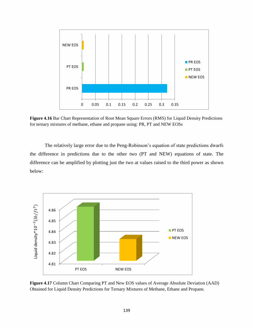
139
Figure 4.16 Bar Chart Representation of Root Mean Square Errors (RMS) for Liquid Density Predictions
for ternary mixtures of methane, ethane and propane using: PR, PT and NEW EOSs
The relatively large error due to the Peng-Robinson’s equation of state predictions dwarfs
the difference in predictions due to the other two (PT and NEW) equations of state. The
difference can be amplified by plotting just the two at values raised to the third power as shown
below:
Figure 4.17 Column Chart Comparing PT and New EOS values of Average Absolute Deviation (AAD)
Obtained for Liquid Density Predictions for Ternary Mixtures of Methane, Ethane and Propane.
0 0.05 0.1 0.15 0.2 0.25 0.3 0.35
PR EOS
PT EOS
NEW EOS
PR EOS
PT EOS
NEW EOS
4.81
4.82
4.83
4.84
4.85
4.86
PT EOS NEW EOS
PT EOS
NEW EOS
Liq
uid
den
sity
*10
−3
( 𝑙𝑏
𝑓𝑡3
⁄)

140
4.4: Application to Four Component (Quaternary) Hydrocarbon Mixtures
The equations of Peng Robinson and Patel-Teja and the New equation of state were used
to calculate densities of the liquid phase and compressibility factors of the vapor or gas phase for
a four component (quaternary) hydrocarbon system. The results are compared with
experimentally measured values for the parameters calculated. The composition of the
quaternary mixture is presented below:
TABLE 4.4a: Composition of Quaternary Simulated Natural gas Mixture
[Source: Biswas, et al., 1990]
Compounds Molecular Weight
𝑀𝑖
Composition, mol. %
Methane
Ethane
Propane
Butane
16.043
30.070
44.097
58.123
80.078
11.641
6.530
1.750
The comparison of the equation of state calculated and experimentally obtained liquid density
results are presented as Table 4.4b(i) below:
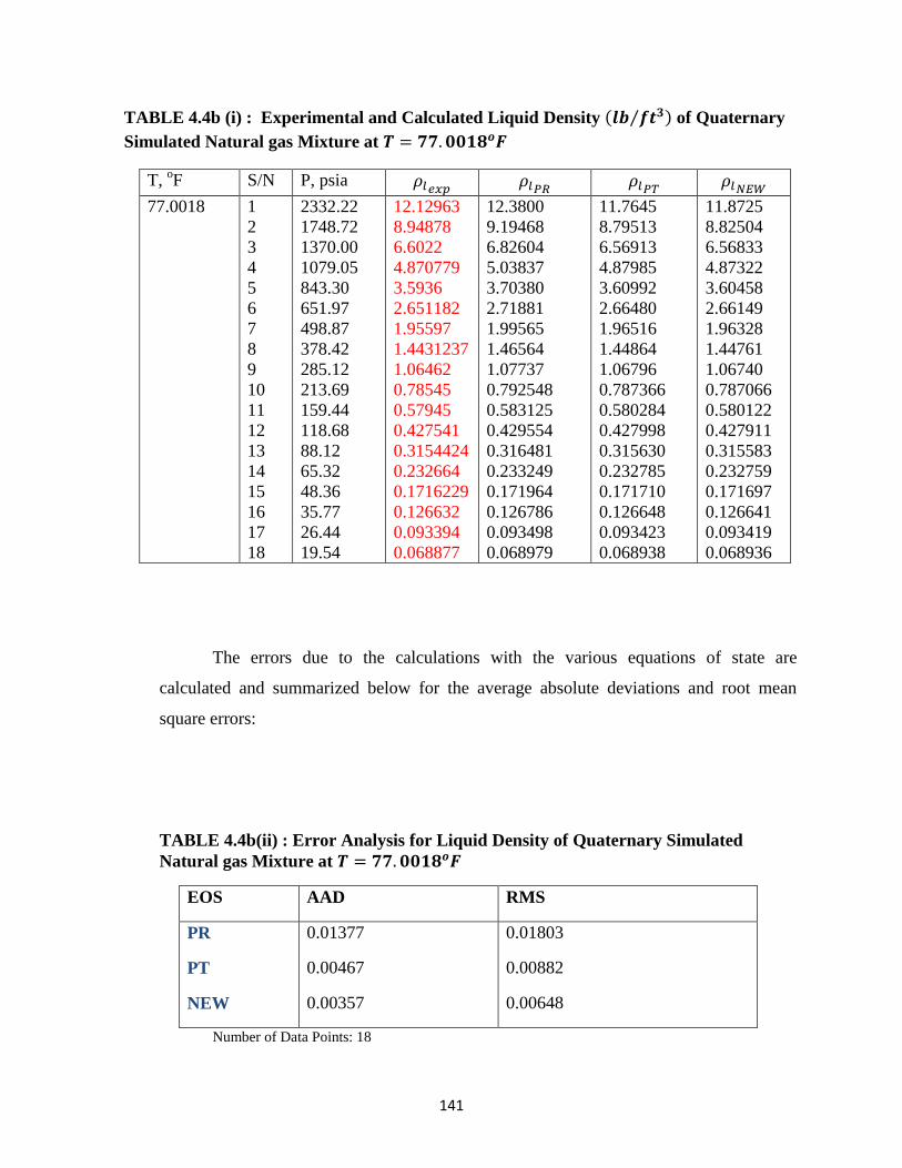
141
TABLE 4.4b (i) : Experimental and Calculated Liquid Density (𝒍𝒃 𝒇𝒕𝟑⁄ ) of Quaternary
Simulated Natural gas Mixture at 𝑻 = 𝟕𝟕. 𝟎𝟎𝟏𝟖𝒐𝑭
T, oF S/N P, psia 𝜌𝑙𝑒𝑥𝑝
𝜌𝑙𝑃𝑅 𝜌𝑙𝑃𝑇
𝜌𝑙𝑁𝐸𝑊
77.0018 1
2
3
4
5
6
7
8
9
10
11
12
13
14
15
16
17
18
2332.22
1748.72
1370.00
1079.05
843.30
651.97
498.87
378.42
285.12
213.69
159.44
118.68
88.12
65.32
48.36
35.77
26.44
19.54
12.12963
8.94878
6.6022
4.870779
3.5936
2.651182
1.95597
1.4431237
1.06462
0.78545
0.57945
0.427541
0.3154424
0.232664
0.1716229
0.126632
0.093394
0.068877
12.3800
9.19468
6.82604
5.03837
3.70380
2.71881
1.99565
1.46564
1.07737
0.792548
0.583125
0.429554
0.316481
0.233249
0.171964
0.126786
0.093498
0.068979
11.7645
8.79513
6.56913
4.87985
3.60992
2.66480
1.96516
1.44864
1.06796
0.787366
0.580284
0.427998
0.315630
0.232785
0.171710
0.126648
0.093423
0.068938
11.8725
8.82504
6.56833
4.87322
3.60458
2.66149
1.96328
1.44761
1.06740
0.787066
0.580122
0.427911
0.315583
0.232759
0.171697
0.126641
0.093419
0.068936
The errors due to the calculations with the various equations of state are
calculated and summarized below for the average absolute deviations and root mean
square errors:
TABLE 4.4b(ii) : Error Analysis for Liquid Density of Quaternary Simulated
Natural gas Mixture at 𝑻 = 𝟕𝟕. 𝟎𝟎𝟏𝟖𝒐𝑭
EOS AAD RMS
PR
PT
NEW
0.01377
0.00467
0.00357
0.01803
0.00882
0.00648
Number of Data Points: 18

142
The New equation of state gives the least average absolute error (0.36%) and least
root mean square error (0.65%). The Peng Robinson’s equation has the highest average
absolute deviation of 1.38% and highest root mean square error of 1.80%. The Patel-Teja
equation of state performs better than the Peng-Robinson’s equation with a significantly
lower value of average absolute deviation (4.67%) and lower root mean square error
(0.88%). The average absolute deviations and root mean square errors are better
appreciated when viewed as pictorial charts as shown below:
Figure 4.18 Column Chart for Average Absolute Deviation (AAD) for Liquid Density
Prediction for Quaternary Simulated Hydrocarbon System Using PR, PT and NEW EOS.
0
0.002
0.004
0.006
0.008
0.01
0.012
0.014
PR EOS PT EOS NEW EOS
PR EOS
PT EOS
NEW EOS
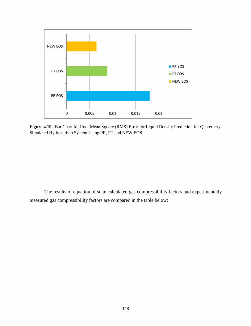
143
Figure 4.19. Bar Chart for Root Mean Square (RMS) Error for Liquid Density Prediction for Quaternary
Simulated Hydrocarbon System Using PR, PT and NEW EOS.
The results of equation of state calculated gas compressibility factors and experimentally
measured gas compressibility factors are compared in the table below:
0 0.005 0.01 0.015 0.02
PR EOS
PT EOS
NEW EOS
PR EOS
PT EOS
NEW EOS
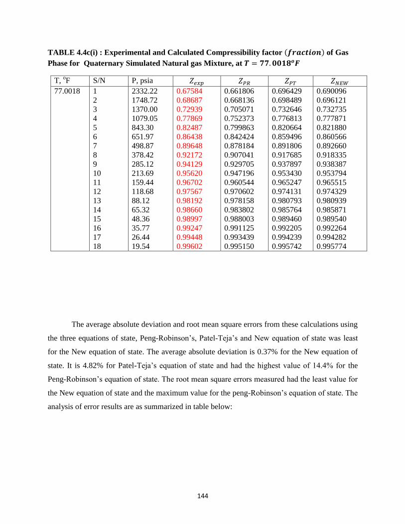
144
TABLE 4.4c(i) : Experimental and Calculated Compressibility factor (𝒇𝒓𝒂𝒄𝒕𝒊𝒐𝒏) of Gas
Phase for Quaternary Simulated Natural gas Mixture, at 𝑻 = 𝟕𝟕. 𝟎𝟎𝟏𝟖𝒐𝑭
T, oF S/N P, psia 𝑍𝑒𝑥𝑝 𝑍𝑃𝑅 𝑍𝑃𝑇 𝑍𝑁𝐸𝑊
77.0018 1
2
3
4
5
6
7
8
9
10
11
12
13
14
15
16
17
18
2332.22
1748.72
1370.00
1079.05
843.30
651.97
498.87
378.42
285.12
213.69
159.44
118.68
88.12
65.32
48.36
35.77
26.44
19.54
0.67584
0.68687
0.72939
0.77869
0.82487
0.86438
0.89648
0.92172
0.94129
0.95620
0.96702
0.97567
0.98192
0.98660
0.98997
0.99247
0.99448
0.99602
0.661806
0.668136
0.705071
0.752373
0.799863
0.842424
0.878184
0.907041
0.929705
0.947196
0.960544
0.970602
0.978158
0.983802
0.988003
0.991125
0.993439
0.995150
0.696429
0.698489
0.732646
0.776813
0.820664
0.859496
0.891806
0.917685
0.937897
0.953430
0.965247
0.974131
0.980793
0.985764
0.989460
0.992205
0.994239
0.995742
0.690096
0.696121
0.732735
0.777871
0.821880
0.860566
0.892660
0.918335
0.938387
0.953794
0.965515
0.974329
0.980939
0.985871
0.989540
0.992264
0.994282
0.995774
The average absolute deviation and root mean square errors from these calculations using
the three equations of state, Peng-Robinson’s, Patel-Teja’s and New equation of state was least
for the New equation of state. The average absolute deviation is 0.37% for the New equation of
state. It is 4.82% for Patel-Teja’s equation of state and had the highest value of 14.4% for the
Peng-Robinson’s equation of state. The root mean square errors measured had the least value for
the New equation of state and the maximum value for the peng-Robinson’s equation of state. The
analysis of error results are as summarized in table below:

145
TABLE 4.4c(ii): Error Analysis on Compressibility Factor Prediction of Quaternary
Simulated Natural gas Mixture at 𝑻 = 𝟕𝟕. 𝟎𝟎𝟏𝟖𝒐𝑭
EOS AAD RMS
PR
PT
NEW
0.01440
0.00482
0.00372
0.01878
0.00854
0.00629
Number of Data Points: 18
Appreciation of these results is enhanced by considering the plot below:
Figure 4.20. Column Chart for Average Absolute Deviation (AAD) for Compressibility factor Prediction
for Quaternary Simulated Hydrocarbon System Using PR, PT and NEW EOS.
0
0.002
0.004
0.006
0.008
0.01
0.012
0.014
0.016
PREOS PT EOS NEW EOS
PREOS
PT EOS
NEW EOS
Ave
rage
Ab
solu
te D
evia
tio
n
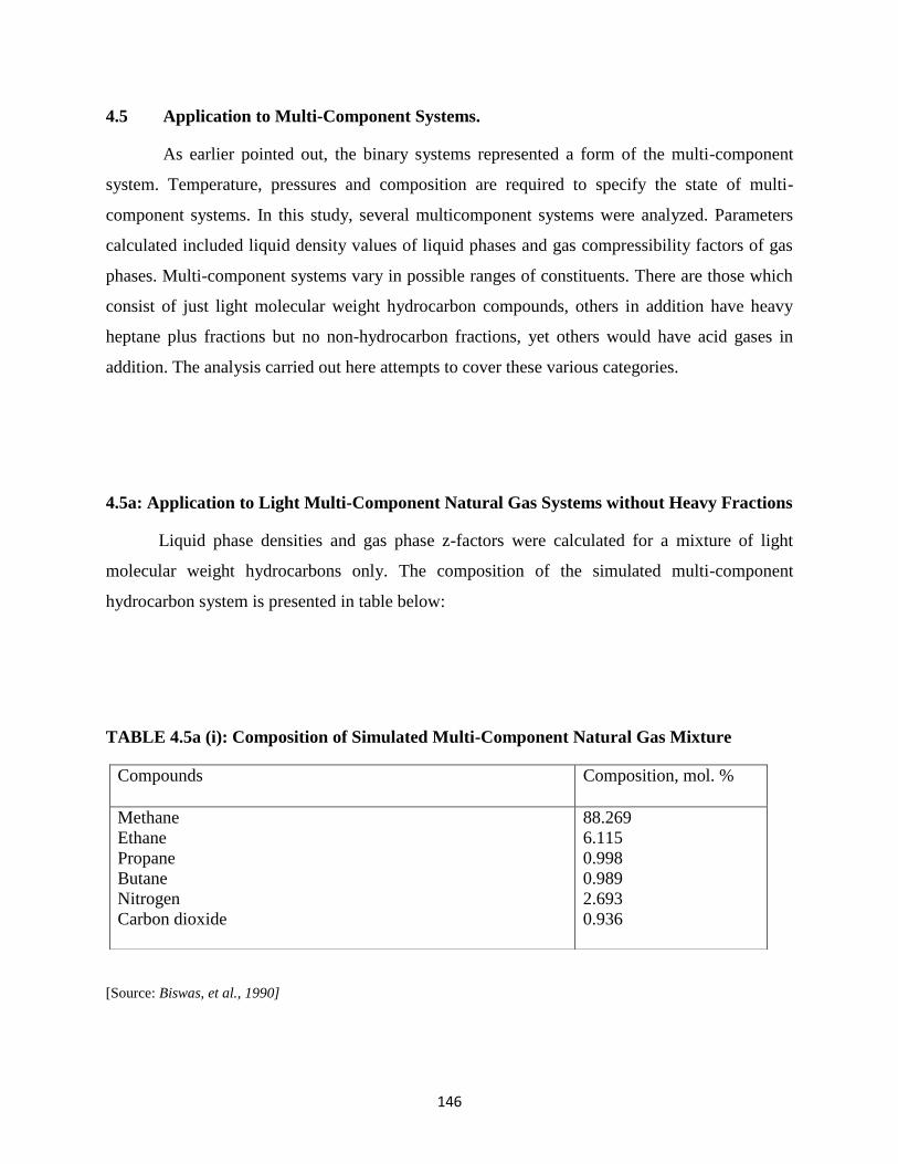
146
4.5 Application to Multi-Component Systems.
As earlier pointed out, the binary systems represented a form of the multi-component
system. Temperature, pressures and composition are required to specify the state of multi-
component systems. In this study, several multicomponent systems were analyzed. Parameters
calculated included liquid density values of liquid phases and gas compressibility factors of gas
phases. Multi-component systems vary in possible ranges of constituents. There are those which
consist of just light molecular weight hydrocarbon compounds, others in addition have heavy
heptane plus fractions but no non-hydrocarbon fractions, yet others would have acid gases in
addition. The analysis carried out here attempts to cover these various categories.
4.5a: Application to Light Multi-Component Natural Gas Systems without Heavy Fractions
Liquid phase densities and gas phase z-factors were calculated for a mixture of light
molecular weight hydrocarbons only. The composition of the simulated multi-component
hydrocarbon system is presented in table below:
TABLE 4.5a (i): Composition of Simulated Multi-Component Natural Gas Mixture
[Source: Biswas, et al., 1990]
Compounds Composition, mol. %
Methane
Ethane
Propane
Butane
Nitrogen
Carbon dioxide
88.269
6.115
0.998
0.989
2.693
0.936
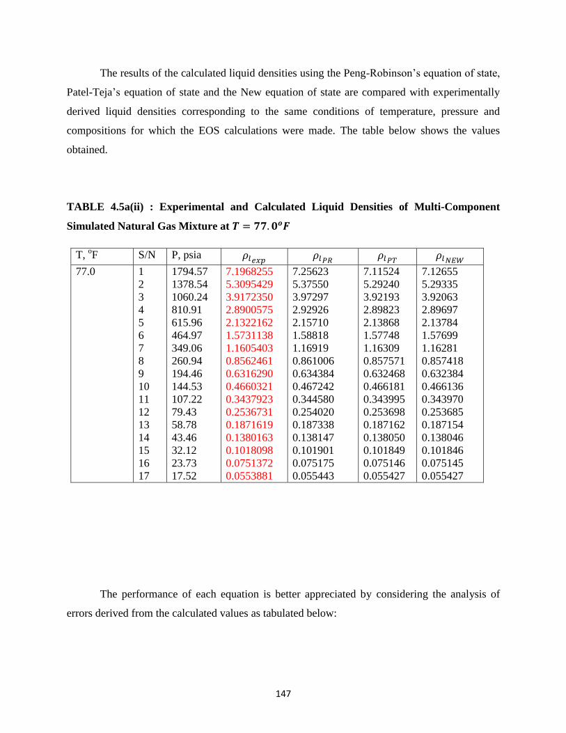
147
The results of the calculated liquid densities using the Peng-Robinson’s equation of state,
Patel-Teja’s equation of state and the New equation of state are compared with experimentally
derived liquid densities corresponding to the same conditions of temperature, pressure and
compositions for which the EOS calculations were made. The table below shows the values
obtained.
TABLE 4.5a(ii) : Experimental and Calculated Liquid Densities of Multi-Component
Simulated Natural Gas Mixture at 𝑻 = 𝟕𝟕. 𝟎𝒐𝑭
T, oF S/N P, psia 𝜌𝑙𝑒𝑥𝑝
𝜌𝑙𝑃𝑅 𝜌𝑙𝑃𝑇
𝜌𝑙𝑁𝐸𝑊
77.0 1
2
3
4
5
6
7
8
9
10
11
12
13
14
15
16
17
1794.57
1378.54
1060.24
810.91
615.96
464.97
349.06
260.94
194.46
144.53
107.22
79.43
58.78
43.46
32.12
23.73
17.52
7.1968255
5.3095429
3.9172350
2.8900575
2.1322162
1.5731138
1.1605403
0.8562461
0.6316290
0.4660321
0.3437923
0.2536731
0.1871619
0.1380163
0.1018098
0.0751372
0.0553881
7.25623
5.37550
3.97297
2.92926
2.15710
1.58818
1.16919
0.861006
0.634384
0.467242
0.344580
0.254020
0.187338
0.138147
0.101901
0.075175
0.055443
7.11524
5.29240
3.92193
2.89823
2.13868
1.57748
1.16309
0.857571
0.632468
0.466181
0.343995
0.253698
0.187162
0.138050
0.101849
0.075146
0.055427
7.12655
5.29335
3.92063
2.89697
2.13784
1.57699
1.16281
0.857418
0.632384
0.466136
0.343970
0.253685
0.187154
0.138046
0.101846
0.075145
0.055427
The performance of each equation is better appreciated by considering the analysis of
errors derived from the calculated values as tabulated below:

148
TABLE 4.5a(iii): Error Analysis for Liquid Density of Simulated Multi-Component
Natural Gas Mixture at 𝑻 = 𝟕𝟕. 𝟎𝟎𝒐𝑭 [Number of Data Points: 17]
EOS AAD RMS
PR
PT
NEW
0.0209
0.0173
0.0170
0.0660
0.0642
0.0641
For liquid density predictions of simulated multi component hydrocarbon system without
heavy ends, the average absolute deviation for the Peng Robinson equation is 2.09%. It is 1.73%
for Patel-Teja’s equation and 1.70% for the New equation. The results show that the New
equation performs better than the Patel-Teja’s equation, though by a small margin. The root
mean square errors (RMS) for Peng Robinson, Patel Teja and New equations were 6.60%, 6.42%
and 6.1%, respectively. For prediction of gas compressibility factors for this system, the Peng
Robinson equation gave an average absolute deviation of 0.61%. Patel-Teja’s equation of state
gave a value of 0.21% and the New equation gave a value of 0.19%. RMS values of 0.791%,
0.33% and 0.28% for PR, PT and New equations were measured.
The same composition of gas is used for the calculation of gas compressibility factors.
Results of calculated and experimentally obtained z-factors are shown in table below for the
simulated multi component system of table 4.5a(i)
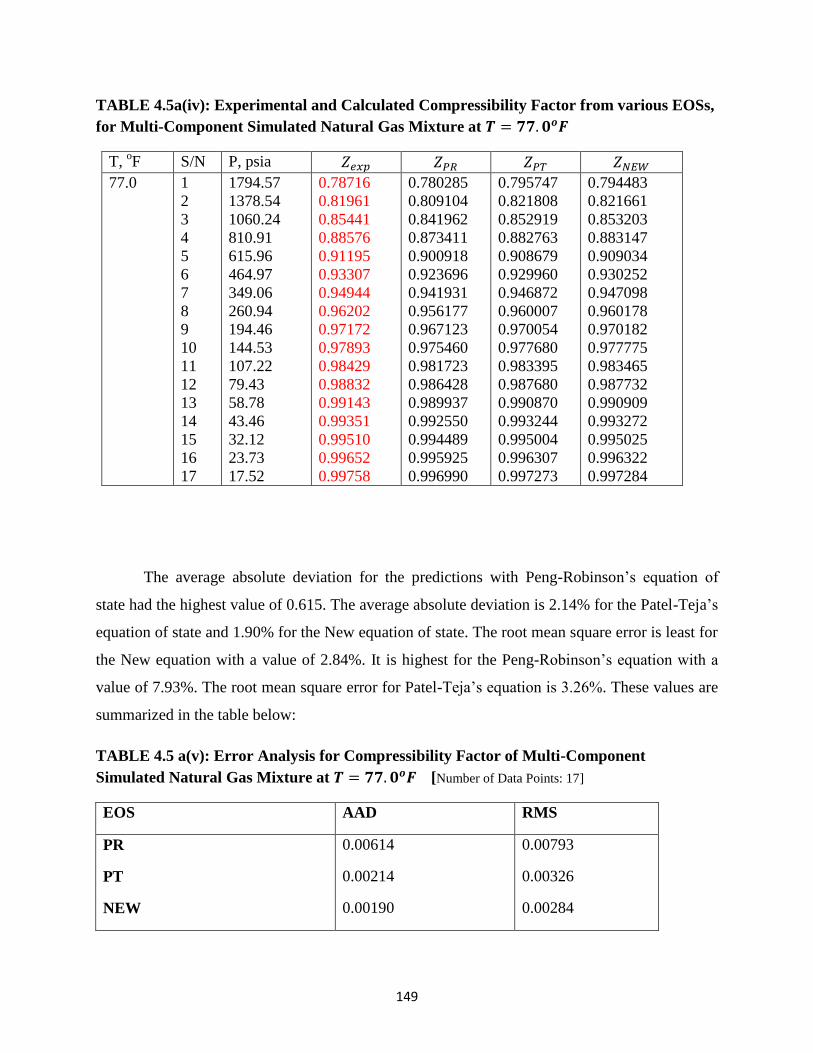
149
TABLE 4.5a(iv): Experimental and Calculated Compressibility Factor from various EOSs,
for Multi-Component Simulated Natural Gas Mixture at 𝑻 = 𝟕𝟕. 𝟎𝒐𝑭
T, oF S/N P, psia 𝑍𝑒𝑥𝑝 𝑍𝑃𝑅 𝑍𝑃𝑇 𝑍𝑁𝐸𝑊
77.0 1
2
3
4
5
6
7
8
9
10
11
12
13
14
15
16
17
1794.57
1378.54
1060.24
810.91
615.96
464.97
349.06
260.94
194.46
144.53
107.22
79.43
58.78
43.46
32.12
23.73
17.52
0.78716
0.81961
0.85441
0.88576
0.91195
0.93307
0.94944
0.96202
0.97172
0.97893
0.98429
0.98832
0.99143
0.99351
0.99510
0.99652
0.99758
0.780285
0.809104
0.841962
0.873411
0.900918
0.923696
0.941931
0.956177
0.967123
0.975460
0.981723
0.986428
0.989937
0.992550
0.994489
0.995925
0.996990
0.795747
0.821808
0.852919
0.882763
0.908679
0.929960
0.946872
0.960007
0.970054
0.977680
0.983395
0.987680
0.990870
0.993244
0.995004
0.996307
0.997273
0.794483
0.821661
0.853203
0.883147
0.909034
0.930252
0.947098
0.960178
0.970182
0.977775
0.983465
0.987732
0.990909
0.993272
0.995025
0.996322
0.997284
The average absolute deviation for the predictions with Peng-Robinson’s equation of
state had the highest value of 0.615. The average absolute deviation is 2.14% for the Patel-Teja’s
equation of state and 1.90% for the New equation of state. The root mean square error is least for
the New equation with a value of 2.84%. It is highest for the Peng-Robinson’s equation with a
value of 7.93%. The root mean square error for Patel-Teja’s equation is 3.26%. These values are
summarized in the table below:
TABLE 4.5 a(v): Error Analysis for Compressibility Factor of Multi-Component
Simulated Natural Gas Mixture at 𝑻 = 𝟕𝟕. 𝟎𝒐𝑭 [Number of Data Points: 17]
EOS AAD RMS
PR
PT
NEW
0.00614
0.00214
0.00190
0.00793
0.00326
0.00284

150
Graphical representations of errors calculated make it easy to assess the performance of
the individual equations of state being compared. Below is a column chart showing the average
absolute deviations for the use of the three equations of state (PR, Pt and New) to calculate
compressibility factors for the Multi-Component Simulated Natural Gas Mixture at 𝑇 = 77.0𝑜𝐹 :
Figure 4.21 Column Chart for Average Absolute Deviation (AAD) for Liquid Density Prediction for
Multi-Component Simulated Natural Gas Mixture at 𝑇 = 77.0𝑜𝐹 Using PR, PT and NEW EOS.
The gas condensate systems with heptane plus fractions that were analyzed were
categorized into four parts: (1) Lean and sweet, (2) carbon dioxide rich and sour (3) poor and
sweet and (4) Highly sour. The terms ‘lean’ refer to gas condensate systems with little
condensable fractions at surface facilities. These are generally systems with low proportions of
C5, C6 and heptane plus fractions. They are richer in methane and light hydrocarbon fractions.
‘Sweet’ refers to mixtures with very little or no hydrogen sulfide fractions. Gases with high
content of hydrogen sulfide are termed ‘Sour’. A gas with little or no condensable fractions
(heavy ends) is termed ‘poor’. ‘Rich’ gases would therefore contain significant amount of
condensable fractions rich in pentane plus fractions.
0
0.001
0.002
0.003
0.004
0.005
0.006
0.007
PR EOS PT EOS NEW EOS
PR EOS
PT EOS
NEW EOS

151
4.5b Application to Gas Condensate Systems Containing Heptane Plus Fractions and Acid
Gases
Gas compressibility factors for Gas condensate systems containing heptane plus fractions
were obtained using the Peng-Robinson’s, Patel-Teja’s and New equation of state. The
composition of the mixtures at varying temperatures and pressures and the calculated and
experimental gas compressibility factors are shown in the table 4.5b(i) below. Following this is
Table 4.5b(ii) which is a tabulation of the errors calculated for the various equation of state
calculations for gas compressibility factors. The value of average absolute deviation for the Peng
Robinson’s equation of state is 5.64%. This is the largest average absolute deviation when
compared to the other two equations. The average absolute deviation is 2.79% for Patel-Teja’s
equation of state calculations. This means that the predictions with the Patel-Teja’s equation of
state are more representative of the experimental results than those of the Peng-Robinson’s
equation of state. By this analogy, the New equation of state gives results that are more
representative of the parameter being measured as it had the lowest average deviation of 1.53%.
The root mean square errors are 5.96%, 3.03% and 2.06% for the Peng-Robinson’s,
Patel-Teja’s and New equation of state, respectively. The error analysis results are summarized
in table 4.5b(ii) shown further down below.

152
TABLE 4.5b (i) Composition of Lean and Sweet Gas Condensate and Gas Compressibility
factor Prediction Results
Reference No.
Composition 281 282 283 284 285 286 287
𝐻2𝑆 0.0000 0.0000 0.0000 0.0000 0.0000 0.0000 0.0000
𝐶𝑂2 0.2310 0.0242 0.0248 0.0253 0.0258 0.0262 0.0266
𝑁2 0.0137 0.0155 0.0161 0.0166 0.0163 0.0155 0.0143
𝐶1 0.6583 0.7074 0.7380 0.7559 0.7583 0.7485 0.7292
𝐶2 0.0803 0.0817 0.0821 0.0839 0.0863 0.0905 0.0944
𝐶3 0.0417 0.0411 0.0404 0.0402 0.0415 0.0447 0.0495
𝑖 − 𝐶4 0.0078 0.0073 0.0070 0.0069 0.0073 0.0082 0.0091
𝑛 − 𝐶4 0.0184 0.0170 0.0162 0.0159 0.0167 0.0186 0.0208
𝑖 − 𝐶5 0.0075 0.0067 0.0062 0.0060 0.0062 0.0070 0.0080
𝑛 − 𝐶5 0.0108 0.0097 0.0089 0.0084 0.0086 0.0096 0.0107
𝑛 − 𝐶6 0.0116 0.0110 0.0103 0.0086 0.0078 0.0082 0.0092
𝐶7+ 0.1268 0.0784 0.0500 0.0323 0.0252 0.0230 0.0282
𝑀𝑜𝑙. 𝑊𝑡 𝐶7+ 191.0 154.0 139.0 128.0 120.0 115.0 113.0
𝑆𝐺. 𝐶7+ 0.831 0.804 0.789 0.778 0.770 0.765 0.763
𝑇𝑒𝑚𝑝. ( 𝐹𝑜 ) 313.0 313.0 313.0 313.0 313.0 313.0 313.0
𝑃 (𝑃𝑠𝑖𝑎) 6010.0 5100.0 4100.0 3000.0 2000.0 1200.0 700.0
𝑃𝑐𝐶7+(𝑃𝑠𝑖𝑎) 324.6 378.4 404.3 427.5 447.2 461.0 466.9
𝑇𝑐𝐶7+( 𝑅𝑜 ) 1264.0 1177.7 1136.4 1105.1 1081.6 1066.6 1060.5
𝑍 −𝑓𝑎𝑐𝑡𝑜𝑟(𝐸𝑥𝑝𝑡. )
1.212 1.075 0.996 0.937 0.930 0.952 0.970
𝑍 −𝑓𝑎𝑐𝑡𝑜𝑟(PR)
1.1314 0.9799 0.9189 0.8915 0.8912 0.9123 0.9356
𝑍 −𝑓𝑎𝑐𝑡𝑜𝑟(PT)
1.1758 1.0234 0.9580 0.9246 0.9175 0.9308 0.9477
𝑍 −𝑓𝑎𝑐𝑡𝑜𝑟(NEW)
1.2666 1.0798 0.9907 0.9395 0.9227 0.9322 0.9481
The results obtained for compressibility factors using the various equations of state when
compared to experimental results show that the new equation of state performs better than the
Peng-Robinson’s and Patel-Teja’s equations for the gas condensate mixtures analyzed. A
summary of the error analysis is shown below. The average absolute deviations for the Peng-
Robinson’s, Patel-Teja’s and New equation of state are respectively, 5.64%, 2.79% and 1.53%.
The average absolute deviations and root mean square errors associated with the various
equations of state are tabulated below:

153
TABLE 4.5 b(ii): Error Analysis of Gas Compressibility Factor Prediction for Lean and
Sweet Gas Condensate
EOS AAD RMS
PR
PT
NEW
0.0564
0.0279
0.0153
0.0596
0.0303
0.0206
An appreciation of the degrees to which the prediction results from the various equations
of state differ from the actual results obtained from experiments is made easier by plotting the
errors associated with each equation either as column or bar charts. A bar chart representation is
shown below the lean and sweet gas:
Figure 4.22 Bar Chart for Root Mean Square Error (RMSE) for Gas Compressibility Factor Predictions
for Lean and Sweet Gas Condensate with Heptane Plus Fractions Using PR, PT and NEW EOS
0 0.01 0.02 0.03 0.04 0.05 0.06 0.07
PR EOS
PT EOS
NEW EOS
PR EOS
PT EOS
NEW EOS

154
The next data set considered is rich in carbon dioxide and also contains heptane plus
fractions. The composition of the fluids and the calculated and experimental gas compressibility
values obtained are given in the table below:
TABLE 4.5b(iii) Composition of Carbon Dioxide-Rich and Sour Gas Condensate and Gas
Compressibility Factor Prediction Results
Reference No.
Composition 926 927 928 929 930 931 932
𝐻2𝑆 0.0030 0.0030 0.0030 0.0030 0.0030 0.0030 0.0040
𝐶𝑂2 0.6352 0.6395 0.6514 0.6579 0.6639 0.6706 0.6716
𝑁2 0.0386 0.0399 0.0410 0.0417 0.0421 0.0411 0.0388
𝐶1 0.1937 0.1988 0.2008 0.2070 0.2084 0.2037 0.1994
𝐶2 0.0303 0.0307 0.0308 0.0309 0.0313 0.0315 0.0318
𝐶3 0.0174 0.0172 0.0170 0.0169 0.0170 0.0145 0.0184
𝑖 − 𝐶4 0.0033 0.0032 0.0031 0.0030 0.0030 0.0032 0.0035
𝑛 − 𝐶4 0.0093 0.0088 0.0085 0.0082 0.0082 0.0088 0.0097
𝑖 − 𝐶5 0.0039 0.0036 0.0033 0.0031 0.0030 0.0033 0.0039
𝑛 − 𝐶5 0.0047 0.0042 0.0038 0.0036 0.0035 0.0038 0.0046
𝑛 − 𝐶6 0.0051 0.0049 0.0046 0.0042 0.0036 0.0030 0.0034
𝐶7+ 0.0551 0.0458 0.0324 0.0202 0.0127 0.0101 0.0113
𝑀𝑜𝑙. 𝑊𝑡 𝐶7+ 170.0 153.0 139.0 128.0 118.0 110.0 106.0
𝑆𝐺. 𝐶7+ 0.811 0.797 0.783 0.773 0.763 0.755 0.751
𝑇𝑒𝑚𝑝. ( 𝐹𝑜 ) 219.0 219.0 219.0 219.0 219.0 219.0 219.0
𝑃 (𝑃𝑠𝑖𝑎) 4825.0 4100.0 3300.0 2600.0 1900.0 1200.0 700.0
𝑃𝑐𝐶7+(𝑃𝑠𝑖𝑎) 347.829 373.929 397.8203 421.6873 446.31732 469.4246 482.3509
𝑇𝑐𝐶7+( 𝑅𝑜 ) 1211.601 1169.445 1131.005 1100.627 1071.227 1046.943 1034.515
𝑍 −𝑓𝑎𝑐𝑡𝑜𝑟(𝐸𝑥𝑝𝑡. )
0.951 0.8276 0.7522 0.7483 0.7882 0.8437 0.8167
𝑍 −𝑓𝑎𝑐𝑡𝑜𝑟(PR)
0.8043 0.7323 0.6866 0.6919 0.7376 0.8160 0.8088
𝑍 −𝑓𝑎𝑐𝑡𝑜𝑟(PT)
0.8236 0.7501 0.7024 0.7069 0.7501 0.8253 0.8181
𝑍 −𝑓𝑎𝑐𝑡𝑜𝑟(NEW)
0.9137 0.8284 0.7611 0.7392 0.7591 0.8320 0.8160
Analysis of the errors for the various equations of state give an average absolute
deviation, (AAD) and root mean square error (RMSE) for the PR EOS were 8.62% and 10.14%,
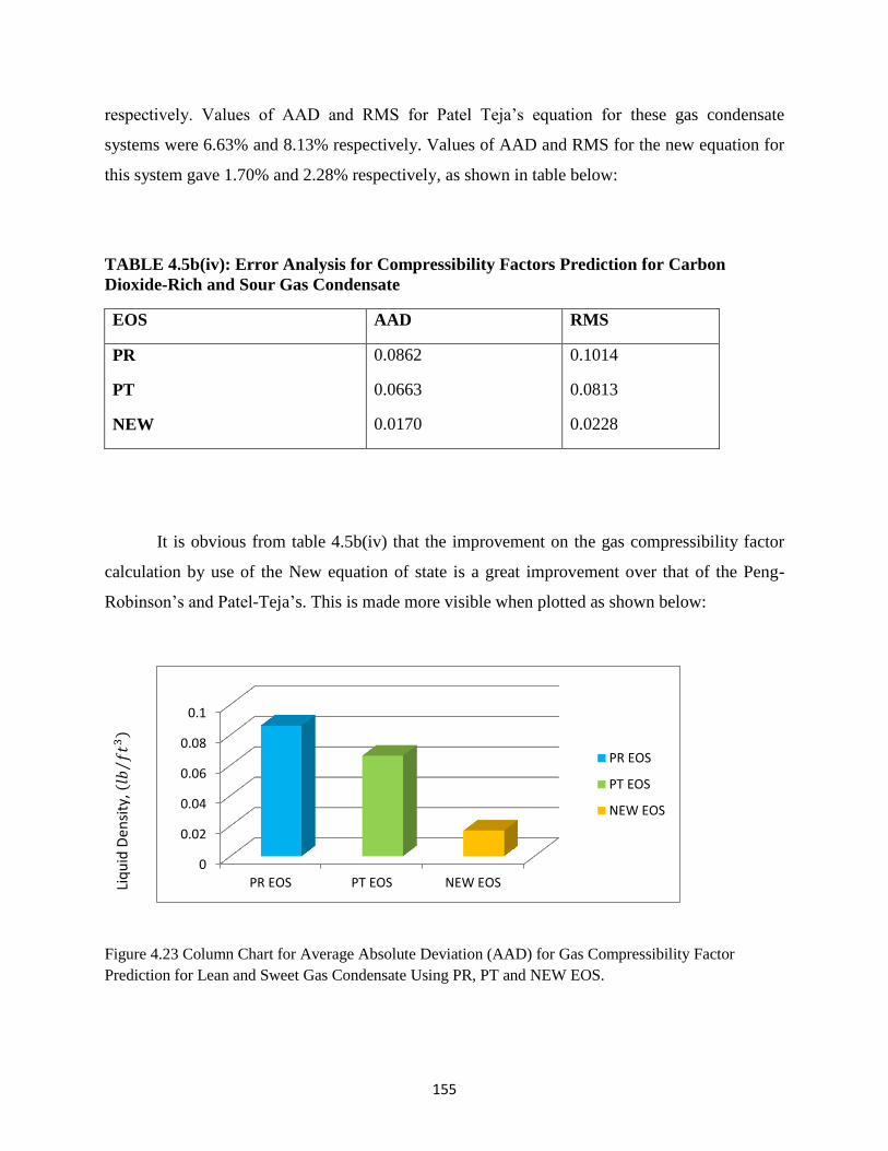
155
respectively. Values of AAD and RMS for Patel Teja’s equation for these gas condensate
systems were 6.63% and 8.13% respectively. Values of AAD and RMS for the new equation for
this system gave 1.70% and 2.28% respectively, as shown in table below:
TABLE 4.5b(iv): Error Analysis for Compressibility Factors Prediction for Carbon
Dioxide-Rich and Sour Gas Condensate
EOS AAD RMS
PR
PT
NEW
0.0862
0.0663
0.0170
0.1014
0.0813
0.0228
It is obvious from table 4.5b(iv) that the improvement on the gas compressibility factor
calculation by use of the New equation of state is a great improvement over that of the Peng-
Robinson’s and Patel-Teja’s. This is made more visible when plotted as shown below:
Figure 4.23 Column Chart for Average Absolute Deviation (AAD) for Gas Compressibility Factor
Prediction for Lean and Sweet Gas Condensate Using PR, PT and NEW EOS.
0
0.02
0.04
0.06
0.08
0.1
PR EOS PT EOS NEW EOS
PR EOS
PT EOS
NEW EOS
Liq
uid
Den
sity
, (𝑙𝑏
𝑓𝑡3
⁄)
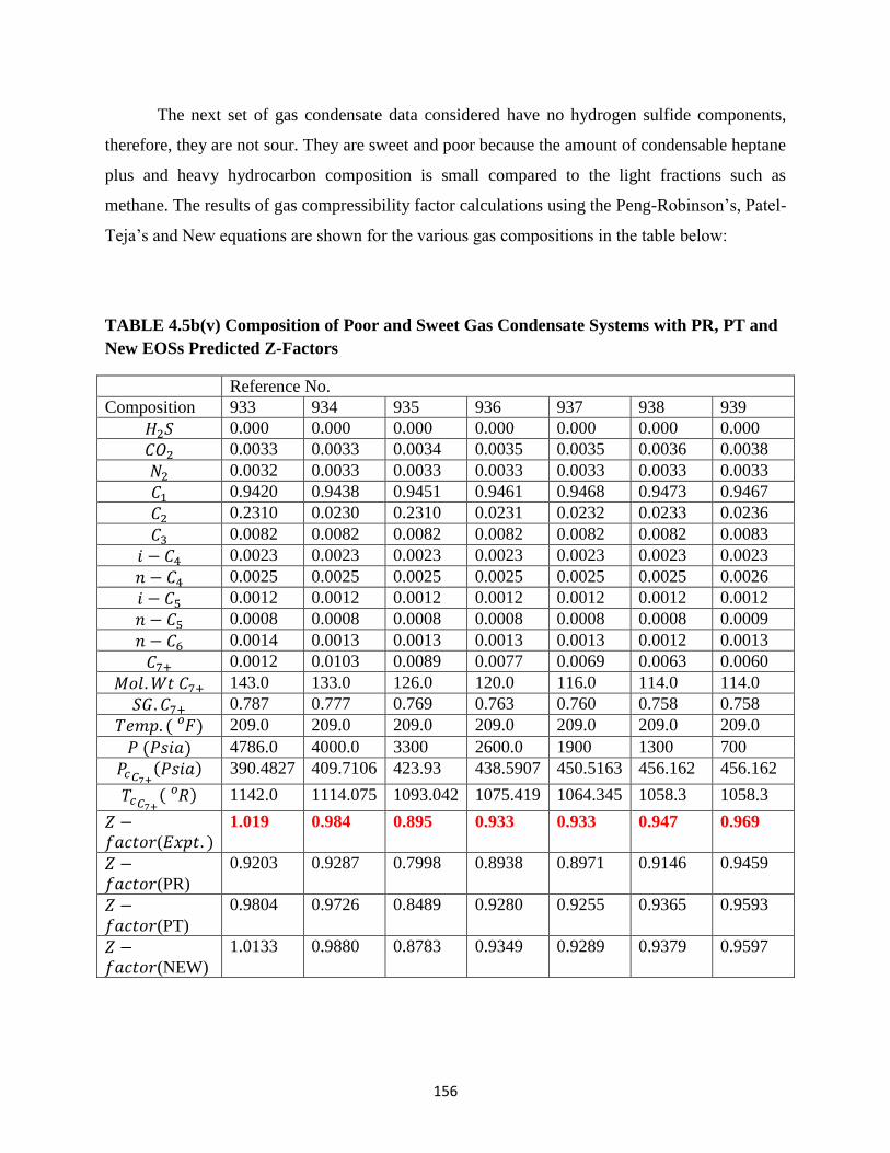
156
The next set of gas condensate data considered have no hydrogen sulfide components,
therefore, they are not sour. They are sweet and poor because the amount of condensable heptane
plus and heavy hydrocarbon composition is small compared to the light fractions such as
methane. The results of gas compressibility factor calculations using the Peng-Robinson’s, Patel-
Teja’s and New equations are shown for the various gas compositions in the table below:
TABLE 4.5b(v) Composition of Poor and Sweet Gas Condensate Systems with PR, PT and
New EOSs Predicted Z-Factors
Reference No.
Composition 933 934 935 936 937 938 939
𝐻2𝑆 0.000 0.000 0.000 0.000 0.000 0.000 0.000
𝐶𝑂2 0.0033 0.0033 0.0034 0.0035 0.0035 0.0036 0.0038
𝑁2 0.0032 0.0033 0.0033 0.0033 0.0033 0.0033 0.0033
𝐶1 0.9420 0.9438 0.9451 0.9461 0.9468 0.9473 0.9467
𝐶2 0.2310 0.0230 0.2310 0.0231 0.0232 0.0233 0.0236
𝐶3 0.0082 0.0082 0.0082 0.0082 0.0082 0.0082 0.0083
𝑖 − 𝐶4 0.0023 0.0023 0.0023 0.0023 0.0023 0.0023 0.0023
𝑛 − 𝐶4 0.0025 0.0025 0.0025 0.0025 0.0025 0.0025 0.0026
𝑖 − 𝐶5 0.0012 0.0012 0.0012 0.0012 0.0012 0.0012 0.0012
𝑛 − 𝐶5 0.0008 0.0008 0.0008 0.0008 0.0008 0.0008 0.0009
𝑛 − 𝐶6 0.0014 0.0013 0.0013 0.0013 0.0013 0.0012 0.0013
𝐶7+ 0.0012 0.0103 0.0089 0.0077 0.0069 0.0063 0.0060
𝑀𝑜𝑙. 𝑊𝑡 𝐶7+ 143.0 133.0 126.0 120.0 116.0 114.0 114.0
𝑆𝐺. 𝐶7+ 0.787 0.777 0.769 0.763 0.760 0.758 0.758
𝑇𝑒𝑚𝑝. ( 𝐹𝑜 ) 209.0 209.0 209.0 209.0 209.0 209.0 209.0
𝑃 (𝑃𝑠𝑖𝑎) 4786.0 4000.0 3300 2600.0 1900 1300 700
𝑃𝑐𝐶7+(𝑃𝑠𝑖𝑎) 390.4827 409.7106 423.93 438.5907 450.5163 456.162 456.162
𝑇𝑐𝐶7+( 𝑅𝑜 ) 1142.0 1114.075 1093.042 1075.419 1064.345 1058.3 1058.3
𝑍 −𝑓𝑎𝑐𝑡𝑜𝑟(𝐸𝑥𝑝𝑡. )
1.019 0.984 0.895 0.933 0.933 0.947 0.969
𝑍 −𝑓𝑎𝑐𝑡𝑜𝑟(PR)
0.9203 0.9287 0.7998 0.8938 0.8971 0.9146 0.9459
𝑍 −𝑓𝑎𝑐𝑡𝑜𝑟(PT)
0.9804 0.9726 0.8489 0.9280 0.9255 0.9365 0.9593
𝑍 −𝑓𝑎𝑐𝑡𝑜𝑟(NEW)
1.0133 0.9880 0.8783 0.9349 0.9289 0.9379 0.9597

157
For this poor and sweet gas condensate system, average absolute deviation (AAD) for
PR, PT and NEW equations of state are, respectively, 6.15%, 1.70% and 0.78%.It is impressive
to note that the New equation reduces the average absolute deviation from a value of 6.15%
obtained with the Peng Robinson’s equation to less than 1.0% at 0.78%. This is a significant
contribution. Root mean square errors (RMSE) for PR, PT and New equation were, 7.01%,
2.28% and 0.94% respectively. Also the difference between the highest RMSE measured by
Peng-Robinson’s equation and that for the New equation of state is a whopping 6.07%. The
summarized results from analysis of the errors are shown in table below:
TABLE 4.5b(vi): Error Analysis for Predicted Z-Factors for Poor and Sweet Gas
Condensate
EOS AAD RMS
PR
PT
NEW
0.0615
0.0170
0.0078
0.0701
0.0228
0.0094
A column chart of the average absolute deviations for the various equations of state are
shown below to emphasize the comparative performance of each equation of state.
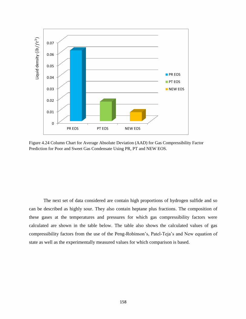
158
Figure 4.24 Column Chart for Average Absolute Deviation (AAD) for Gas Compressibility Factor
Prediction for Poor and Sweet Gas Condensate Using PR, PT and NEW EOS.
The next set of data considered are contain high proportions of hydrogen sulfide and so
can be described as highly sour. They also contain heptane plus fractions. The composition of
these gases at the temperatures and pressures for which gas compressibility factors were
calculated are shown in the table below. The table also shows the calculated values of gas
compressibility factors from the use of the Peng-Robinson’s, Patel-Teja’s and New equation of
state as well as the experimentally measured values for which comparison is based.
0
0.01
0.02
0.03
0.04
0.05
0.06
0.07
PR EOS PT EOS NEW EOS
PR EOS
PT EOS
NEW EOS
Liq
uid
den
sity
(𝑙𝑏
𝑓𝑡3
⁄)
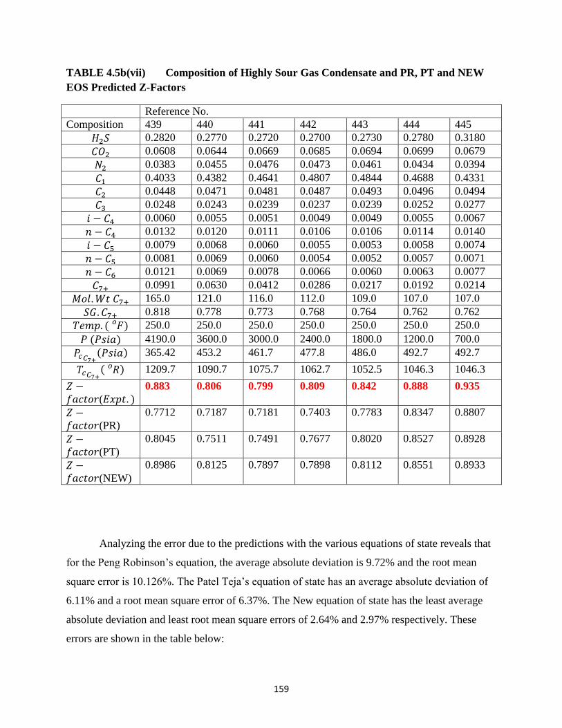
159
TABLE 4.5b(vii) Composition of Highly Sour Gas Condensate and PR, PT and NEW
EOS Predicted Z-Factors
Reference No.
Composition 439 440 441 442 443 444 445
𝐻2𝑆 0.2820 0.2770 0.2720 0.2700 0.2730 0.2780 0.3180
𝐶𝑂2 0.0608 0.0644 0.0669 0.0685 0.0694 0.0699 0.0679
𝑁2 0.0383 0.0455 0.0476 0.0473 0.0461 0.0434 0.0394
𝐶1 0.4033 0.4382 0.4641 0.4807 0.4844 0.4688 0.4331
𝐶2 0.0448 0.0471 0.0481 0.0487 0.0493 0.0496 0.0494
𝐶3 0.0248 0.0243 0.0239 0.0237 0.0239 0.0252 0.0277
𝑖 − 𝐶4 0.0060 0.0055 0.0051 0.0049 0.0049 0.0055 0.0067
𝑛 − 𝐶4 0.0132 0.0120 0.0111 0.0106 0.0106 0.0114 0.0140
𝑖 − 𝐶5 0.0079 0.0068 0.0060 0.0055 0.0053 0.0058 0.0074
𝑛 − 𝐶5 0.0081 0.0069 0.0060 0.0054 0.0052 0.0057 0.0071
𝑛 − 𝐶6 0.0121 0.0069 0.0078 0.0066 0.0060 0.0063 0.0077
𝐶7+ 0.0991 0.0630 0.0412 0.0286 0.0217 0.0192 0.0214
𝑀𝑜𝑙. 𝑊𝑡 𝐶7+ 165.0 121.0 116.0 112.0 109.0 107.0 107.0
𝑆𝐺. 𝐶7+ 0.818 0.778 0.773 0.768 0.764 0.762 0.762
𝑇𝑒𝑚𝑝. ( 𝐹𝑜 ) 250.0 250.0 250.0 250.0 250.0 250.0 250.0
𝑃 (𝑃𝑠𝑖𝑎) 4190.0 3600.0 3000.0 2400.0 1800.0 1200.0 700.0
𝑃𝑐𝐶7+(𝑃𝑠𝑖𝑎) 365.42 453.2 461.7 477.8 486.0 492.7 492.7
𝑇𝑐𝐶7+( 𝑅𝑜 ) 1209.7 1090.7 1075.7 1062.7 1052.5 1046.3 1046.3
𝑍 −𝑓𝑎𝑐𝑡𝑜𝑟(𝐸𝑥𝑝𝑡. )
0.883 0.806 0.799 0.809 0.842 0.888 0.935
𝑍 −𝑓𝑎𝑐𝑡𝑜𝑟(PR)
0.7712 0.7187 0.7181 0.7403 0.7783 0.8347 0.8807
𝑍 −𝑓𝑎𝑐𝑡𝑜𝑟(PT)
0.8045
0.7511 0.7491 0.7677 0.8020 0.8527 0.8928
𝑍 −𝑓𝑎𝑐𝑡𝑜𝑟(NEW)
0.8986 0.8125 0.7897 0.7898 0.8112 0.8551 0.8933
Analyzing the error due to the predictions with the various equations of state reveals that
for the Peng Robinson’s equation, the average absolute deviation is 9.72% and the root mean
square error is 10.126%. The Patel Teja’s equation of state has an average absolute deviation of
6.11% and a root mean square error of 6.37%. The New equation of state has the least average
absolute deviation and least root mean square errors of 2.64% and 2.97% respectively. These
errors are shown in the table below:

160
TABLE 4.5 b(viii): Error Analysis for Z-Factor Predictions for Poor and Sweet Gas
Condensate
EOS AAD RMS
PR
PT
NEW
0.0972
0.0611
0.0264
0.1016
0.0637
0.0297
Considering all the gas condensate systems for which gas compressibility factors were
calculated, the overall average absolute deviations and root mean square errors are calculated and
presented as table 4.5b(ix) below:
TABLE 4.5b(ix) : Summary of Errors Analyzed for Gas Condensate Systems with Heptane
Plus Fractions and Acid Gases
Equation of State Peng Robinson Patel-Teja New
AAD: 4.5𝑐(𝑣)
4.5𝑐(𝑣𝑖)
4.5𝑐(𝑣𝑖𝑖)
4.5𝑐(𝑣𝑖𝑖𝑖)
0.0564
0.0862
0.0615
0.0972
0.0279
0.0663
0.0170
0.0611
0.0153
0.0170
0.0078
0.0264
TOTAL 0.07532 0.0454 0.0033
RMS: 4.5𝑐(𝑣)
4.5𝑐(𝑣𝑖)
4.5𝑐(𝑣𝑖𝑖)
4.5𝑐(𝑣𝑖𝑖𝑖)
0.0596
0.1014
0.0701
0.1016
0.0303
0.0813
0.0228
0.0637
0.0206
0.0228
0.0094
0.0297
TOTAL 0.0073 0.0033 0.0005

161
In general terms, the lowest average absolute deviation was obtained as 0.78% with the
New equation of state for the gas condensate system described as poor and sweet for which
hydrogen sulfide concentration is 0.0%, methane concentration is greater than 90%, carbon
dioxide concentration is equal to about 0.32% and heptane plus fractions are less than 1.1%. The
smallest value of root mean square error of 0.94% was also measured with the new equation of
state for this group of condensates.
The highest average absolute deviation of 9.72% was obtained for the Peng Robinson’s
equation of state predictions for the highly sour gas condensate systems. This group is
characterized by following constituent compositions: 𝐻2𝑆 > 0.27, 0.060 < 𝑚𝑜𝑙 𝐶𝑂2 < 0.069,
0.038 < 𝑚𝑜𝑙 𝑁2 < 0.048, 0.4033 < 𝑚𝑜𝑙 𝐶𝐻4 < 0.4033 and 0.02 < 𝑚𝑜𝑙 𝐶7+ < 0.09. The
highest average absolute deviation for predictions made with the new equation of state was also
got as 2.64% for this group of gas condensate systems.
4.6 Performance of Riazi-Daubert Correlation for Predicting Critical Pressures of
Heptane Plus Fractions
The Riazi-Daubert correlation which is an excellent correlation for calculating critical
properties of heptane plus fractions was found however, to show significant deviation from
accuracy for fractions in the range of specific gravity: 0.770 ≤ 𝑆𝐺𝐶7+ ≤ 0.850. The final results
of values predicted with equations of state are impacted by the values of parameters used for
such calculations, such as the critical temperatures and pressures for each of the components in
the mixture. To ensure consistency in accurate equation of state performances, this weakness
shown by the Riazi-Daubert correlation, which is adopted for all heptane plus calculations used
in this study, a New correlation was developed to be used with the Riazi-Daubert correlation at
its region of weakness. The performance of the New correlation is compared with that of Riazi-
Daubert at the range 0.770 ≤ 𝑆𝐺𝐶7+ ≤ 0.850 in the table below:
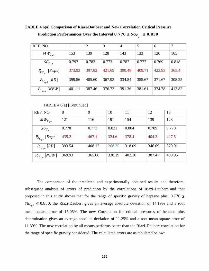
162
TABLE 4.6(a) Comparison of Riazi-Daubert and New Correlation Critical Pressure
Prediction Performances Over the Interval 𝟎. 𝟕𝟕𝟎 ≤ 𝑺𝑮𝑪𝟕+ ≤ 𝟎. 𝟖𝟓𝟎
REF. NO. 1 2 3 4 5 6 7
𝑀𝑊𝐶7+ 153 139 128 143 133 126 165
𝑆𝐺𝐶7+ 0.797 0.783 0.773 0.787 0.777 0.769 0.818
𝑃𝑐𝐶7+
[𝐸𝑥𝑝𝑡] 373.93 397.82 421.69 390.48 409.71 423.93 365.4
𝑃𝑐𝐶7+
[𝑅𝐷] 399.56 405.60 367.93 334.84 355.67 371.67 308.25
𝑃𝑐𝐶7+
[𝑁𝐸𝑊] 401.11 387.46 376.73 391.36 381.61 374.78 412.82
TABLE 4.6(a) [Continued]
REF. NO. 8 9 10 11 12 13
𝑀𝑊𝐶7+ 121 116 191 154 139 128
𝑆𝐺𝐶7+ 0.778 0.773 0.831 0.804 0.789 0.778
𝑃𝑐𝐶7+
[𝐸𝑥𝑝𝑡] 435.2 467.1 324.6 378.4 404.3 427.5
𝑃𝑐𝐶7+
[𝑅𝐷] 393.54 408.12 268.25 318.09 346.09 370.91
𝑃𝑐𝐶7+
[𝑁𝐸𝑊] 369.93 365.06 338.19 402.10 387.47 409.95
The comparison of the predicted and experimentally obtained results and therefore,
subsequent analysis of errors of prediction by the correlations of Riazi-Daubert and that
proposed in this study shows that for the range of specific gravity of heptane plus, 0.770 ≤
𝑆𝐺𝐶7+ ≤ 0.850, the Riazi-Daubert gives an average absolute deviation of 14.19% and a root
mean square error of 15.05%. The new Correlation for critical pressures of heptane plus
determination gives an average absolute deviation of 11.25% and a root mean square error of
11.39%. The new correlation by all means performs better than the Riazi-Daubert correlation for
the range of specific gravity considered. The calculated errors are as tabulated below:

163
TABLE 4.6(b) Error Analysis on Critical Pressure Predictions for Heptane Plus Fractions
CORRELATION 𝐴𝐴𝐷 𝑅𝑀𝑆
Riazi-Daubert 0.1419 0.1505
NEW 0.1125 0.1139
4.7 Statistical Methods Used for Error Analysis
Comparison is made easy by use of the statistical methods of absolute average deviation
(AAD) and root mean square deviation (RMS). By definition,
1. Absolute Average Deviation: 𝐴𝐴𝐷 =1
𝑛∑ |(
𝑋𝑒𝑥𝑝𝑒𝑟𝑖𝑚𝑒𝑛𝑡𝑎𝑙−𝑋𝑐𝑎𝑙𝑐𝑢𝑙𝑎𝑡𝑒𝑑
𝑋𝑐𝑎𝑙𝑐𝑢𝑙𝑎𝑡𝑒𝑑)|𝑛
𝑖=1 , and
2. Root Mean Square Deviation: 𝑅𝑀𝑆 = √1
𝑛∑ ((
𝑋𝑒𝑥𝑝𝑒𝑟𝑖𝑚𝑒𝑛𝑡𝑎𝑙−𝑋𝑐𝑎𝑙𝑐𝑢𝑙𝑎𝑡𝑒𝑑
𝑋𝑐𝑎𝑙𝑐𝑢𝑙𝑎𝑡𝑒𝑑))
2
𝑛𝑖=1
164
CHAPTER FIVE
5.0 CONCLUSIONS AND RECOMMENDATIONS
A number of inferences to be drawn from the study and recommendations based on the
findings are discussed below:
5.1 CONCLUSIONS
1. By using provable analytical technique, a new equation of state capable of minimizing
bias between the experimentally measured and equation of state estimated values of
liquid densities, beyond that afforded by the Peng-Robinson’s and Patel-Teja’s EOSs has
been developed.
2. The new equation is the first in attempting to put the proposal of Yun et al. (1998) to test
in terms of improving equation of state performance based on representation of its virial
coefficients.
3. This study showed how three parameter equations of state can be made amenable to
solution with the Coats generalized form which has only been applied to two parameter
equations of state.
4. The New equation of state gives better hydrocarbon liquid and vapor property predictions
than Peng Robinson’s and Patel-Teja’s equations.
5. The proposed EOS performs better than the Peng Robinson’s and Patel Teja’s equations
of state at regions close to critical point conditions.
6. The New equation of state eliminates the need for incorporating binary interaction
coefficients without compromising accuracy of predictions significantly.
7. The proposed equation of state shows significant predictive abilities over a wide range of
temperature, pressure and for varied fluid types.
8. The presence of acid gases in high concentrations in particular, reduces the ability of
equations of state to in predicting volumetric and equilibrium properties. The effect of the
presence of acid gases at low concentrations does not significantly affect prediction
results.
9. A new correlation that improved critical pressure estimation for Heptane plus fractions
(𝑃𝑐 𝐶7+
) over the range where the Riazi-Daubert correlation weakens is presented.
165
5.2 RECOMMENDATIONS
1. With the demonstrated improvement in the predictive capability of the proposed EOS
over the industry popular two-parameter PR EOS and three-parameter PT EOS, the new EOS is
therefore, strongly recommended for calculating the volumetric properties of natural gas and gas
condensate systems.
2. The inclusion of an additional term in the 𝜋(𝑣) 𝑓𝑢𝑛𝑐𝑡𝑖𝑜𝑛, say 𝑚
𝑉3 should be experimented
upon by another researcher to see the degree, if any, of further improvements
3. The fact that the New equation of state, as does the Peng Robinson and Patel-Teja’s
equations of state show weakness in prediction capabilities when the undefined heptane plus
fractions and acid gases form part of the gas composition may be ameliorated, perhaps by use of
binary interaction coefficients. This can be an area of further research in future.
4. Gas mixtures in which inert gases, such as helium, form part of the overall composition
should be analyzed to see the overall effect of the inert gases if any when equation of state
derived properties are compared with experimentally derived results. Experiments may be
carried out to provide experimental data for comparisons for reason of paucity or lack of data
from literature.
3. There is no evidence in literature of any correlation that calculates the influence of acid
gas fractions on gas condensate mixture on a unit basis, that is effect on one component at a tie
and not the entire mixture. The popular correlation by Wichert and Aziz which correct for effect
of acid gases is applicable for use in calculating adjusted compressibility factor using charts,
tables, graphs or other correlations but is not applicable on a per compound basis but applies to
entire gas mixture. They cannot therefore, be used with numerical models such as equations of
state (see table 4.5c). This is because the adjustments to the critical pressure and temperature as a
result of the acid gases applies to the entire fluid and not to the individual components therefore,
determining parameters such as critical reduced temperatures and reduced pressures for
individual components as are applicable in EOS models is not attainable. Therefore, its
application in numerical analysis is not possible. It is recommended that a correlation which
tackles this obvious and grievous problem be developed.

166
4. The New equation of state has been validated using single components and multi-
components of various complexities. Its application to phase envelope generation, calculation of
liquid holdup and full compositional analysis are areas where further studies could be carried out
to accentuate the relative merits recorded so far.
REFERENCES
1. Adachi, Y., Lu, B. C. Y. and Sugie, H. (1983). “A Four-Parameter Equation of State”,
Fluid Phase Equilib., 11, 29-48.
2. Adewumi, M. A. (2014), PNG 520: Online Course on, “Phase Relations in Reservoir
Engineering”, https://www.e-education.psu.edu/png520/ml_p4.html
3. Ahmed, T. K.(1986). “Comparative Study of Eight Equations of State for Predicting
Hydrocarbon Volumetric Phase Behavior”.
4. Ayala, L. F., (2006) Lecture Notes on PNG 520: Phase Behavior of Hydrocarbon
Fluids. The Pennsylvania State University.
5. Bakker R. J. and Diamond L. W. (2000) “Determination of the composition and
volume of 𝐻2𝑂 − 𝐶𝑂2 fluid inclusions by microthermometry”. Geochim. Cosmochim.
Acta 64, 1753-1764.
6. Benedict, M.; Webb, G. B.; Rubin, L. C. (1940), "An Empirical Equation for
Thermodynamic Properties of Light Hydrocarbons and Their Mixtures: I. Methane,
Ethane, Propane, and n-Butane", Journal of Chemical Physics 8 (4): 334–345,
Bibcode:1940JChPh...8..334B, doi:10.1063/1.1750658, ISSN 0021-9606.
7. Biswas, S. N., Bominaar, S. A. R. C., Schouten, J. A. Michels, J. P. J. and Seldam,
C. A. (1990) “Compressibility isotherms of Simulated natural Gases”, J. Chem. Eng.
Data, 35, 35-38.
8. Boublik, T. (1981). Statistical Thermodynamics of Non-spherical Molecule Fluids.
Ber. Bunsenges, Phys. Chem. 85,1038-1041.

167
9. Carnahan, N. F. and Starling, K. E. (1969). Equation of State for Non-attracting Rigid
Spheres, J. Chem. Phys., 51, 635-636.
10. Coats, K.H. (1985). “Simulation of Gas Condensate Reservoir Performance”, SPE
Paper 10512, Journal of Petroleum Technology.
11. Danesh A. (1998). “PVT and Phase Behavior of Petroleum Reservoir Fluids”, Elsevier
Science, Second Edition, Amsterdam.
12. Elsharkawy, A. M. (2004): “Efficient Methods for Calculations of Compressibility,
Density and Viscosity of natural Gases”, Fluid Phase Equilibria, 218, 1-13.
13. Esmaeilzadeh F., Roshanfekr M. (2004). “A new Cubic Equation of State for
Reservoir Fluids”, Fluid Phase Equilibria Vol.(239): 83–90
14. Firoozabadi A. (1989), “Thermodynamics of Hydrocarbon Reservoirs”, McGraw-Hill.
15. Guggenheim, E. A. (1965). “Variations on van der Waals’ Equation of State for High
Densities”, Mol. Phys., 9, 199-200.
16. Guo, T.M., Du, L., (1989), “A three-parameter cubic equation of state for reservoir
fluids”, Fluid Phase Equilibria, vol. 5, no. 1: p. 47-51.
17. Harmens, A and Knapp, H. (1980) “Three-Parameter Cubic Equation of State for
Normal Substances”, Ind. Eng. Chem. Fund. 19. P. 291-294.
18. Jacobsen, R. T., Penoncello, S. G., Lemmon, E. W. and Span, R.(2000): “Multi-
parameter equation of state”, in Sengers, J. V., Kayser, R. F., Peters, C. J., White Jr. H.
J. (Eds.), Equation of State of Fluids and Fluid Mixtures, Elsevier, Amsterdam, 849-
881.
19. Kahre, L. C. (1973). “Liquid Density of Light Hydrocarbon Mixtures”, Journal of
Chemical and Engineering Data, Vol. 18, No. 3, 1973, pg. 267-270.
20. Kamerlingh Onnes, H., (1902), “Expression of the equation of state of gases and
liquids by means of series”, in: KNAW, Proceeding, 4, Amsterdam, p. 125-147.
21. Kesler, M. G., and Lee, B. I. (1976): “Improved Predictions of Enthalpy of Fractions”.
Hydro. Proc., 55, 153.
22. Kolafa, J. and Nezbeda, I. (1994). “Lennard-Jones Fluid: An Accurate Analytic and
Theoretically-Based equation of State”, Fluid Phase equilib., 100, 1-34.
23. McCain, W. D. Jr.,(1994) “Volatile Oils and retrograde Gases-What’s the difference?”
Petroleum Engineering International. Vol. 35

168
24. Martin, J. J., (1979), “Cubic Equations of State-Which?” Ind. Eng. Chem. Fund.,
18(2), 81-97.
25. Mathews, T. A., Roland, C. H. and Katz, D. L. (1942): “High Pressure Gas
Measurement”, Petroleum Refiner, 21, No. 6, 58.
26. Maxwell, J.C. (1875). “van der Waals on the continuity of the gaseous and liquid
states”. Scientific Papers, Vol. II.p.407-416.
27. Mehra, R. K., Heidemann, R. A., and Aziz, K., (1983),: “An Accelerated Successive
Substitution Algorithm”, Canadian J. of Chemical Engineering, vol. 16, 590-596.
28. Moran and Shapiro,(2000). “Fundamentals of Engineering Thermodynamics”, Wiley,
4th Ed.
29. Mohr, P. J., Taylor, B. N. and Newell, D. B.: (2008) “CODATA recommended values
of the Fundamental Physical Constants: 2006. J. Phys. Chem. Ref. data, 37, p.1187-
1284. Http://physics.nist.gov/cuu/Constants/index.html
30. Nasrifar, Kh. And Bolland, O. (2006): “Prediction of thermodynamic properties of
natural gas mixtures using 10 equations of state including a new cubic two-constant
equation of state”. Journal of Petroleum Science and Engineering, 51, 253-266
31. O’Connell, J. P. and Haile, J. M. (2005):”Thermodynamics, Fundamentals for
applications”, Cambridge University Press, New York. Pg 17
32. Patel, N. C. & Teja, A. S. (1982). “A New Cubic Equation of State for Fluids and
Fluid Mixtures”, Chem. Eng. Sci., Vol. 37, 463-473.
33. Peng, D. Y., and Robinson, D. B. (1976). "A New Two-Constant Equation of State".
Ind. and Eng. Chem. Fundam. 15: No.1,p. 59–64.
34. Piper, L. D., McCain Jr., W. D., and Corredor, J. H. (1993). “Compressibility Factors
for Naturally Occurring Petroleum Gases Paper SPE 26668 Presented at the SPE
Annual Technical Conference and Exhibition, Houston, Tx. 3-6 October.
MS. http://dx.doi.org/10.2118/26668-MS
35. Pitzer, K. S. (1995). “Thermodynamics”, (third ed.). New York: McGraw-Hill.
ISBN 0-07-050221-8.
36. Rachford, H. H. and Rice, J. D. (1952): “Procedure for Use of Electrical Digital
Computers in Calculating Flash Vaporization Hydrocarbon Equilibrium”, Journal of
Petroleum Technology, Technical Note 136, p 19.

169
37. Redlich, O. and Kwong, J. N. S. (1949). “On The Thermodynamics of
Solutions”.Chem. Rev. 44(1). P. 233-244
38. Redlich, O., (1975). "On the Three-Parameter Representation of the Equation of
State". Industrial & Engineering Chemistry Fundamentals 14 (3): 257–260.
doi:10.1021/i160055a020. Retrieved 6 May 2012.
39. Reif-Acherman, S. (2008). "Joseph Neng Shun Kwong: A Famous and Obscure
Scientist". Quim. Nova. 31 (7): 1909–1911. doi:10.1590/S0100-40422008000700054.
40. Reiss, N. R., Frisch, H. L. and Lebowitz, J. L. L. (1959). Statistical Mechanics of
Rigid Spheres, J. Chem. Phys., 31, 369-380.
41. Riazi, M. R., and Daubert, T. E. (1987),:”Characterization Parameters for Petroleum
Fractions”, Ind. Eng. Chem. Res. Vol. (26), 755-759.
42. Risnes, R., Dalen, V. and Jessen, J. I., (1981): “Phase Equilibrium Calculations in the
Near-Critical Region”, Elsevier Sequoia, SA, Proceedings of the European
Symposium on EOR, 329-350, Lausanne.
43. Schmidt G. and Wenzel H. (1980), A Modified van der Waals type equation of State,
Chem. Eng. Sci, 35,p. 1503-1512.
44. Scott, R. L., (1970). Eyring, H., Henderseon, D. and Jost, W. (Eds.), In Physical
Chemistry, An Advanced Treatise, Vol. 8A: Liquid State, Academic Press, New York.
45. Sengers, J. V., Kayser, C. J. Peters, White Jr. H. J. (ed.). (2000) “Equations of State for
Fluids and Fluid Mixtures”, International Union of Pure and Applied chemistry. p. 78.
46. Shana’a, M. Y. and Canfield, F. B. (1968). “Liquid Density and Excess Volume of
Light Hydrocarbon Mixtures at −165.00𝑜𝐶”, Transactions of the Faraday Society, 64.
p. 23-28.
47. Sim, W. J. and Daubert, T. E.(1980), “Prediction of Vapor-Liquid Equilibria of
Undefined Mixtures,Eng. Chem. Process Des. Dev., 19, No. 3.
48. Soave, G., (1972), “Equilibrium Constants from a Modified Redlich-Kwong Equation
of State”. Chem. Eng. Sci., 27,p.1197-1203
49. Standing, M. B., (1981): “Volumetric and Phase Behavior of Oil Field Hydrocarbon
Systems”, 9th
Printing, Society of Petroleum Engineers of AIME, Dallas, Texas.

170
50. Standing, M. B. and Katz, D. L. (1942), “Density of Natural Gases”, In Transaction of
the American Institute of Mining and Metallurgical Engineers, No. 142, SPE-942140-
G. New York:. AIME. 146, p.144
51. Stryjek, R. and Vera, L. H. (1986). PRSV: An Improved Peng-Robinson Equation of
State for Pure Compounds and Mixtures, Can. J. Chem. Eng., 64, p.323-340.
52. Sutton, R. P.(1985): “Compressibility Factors for High Molecular Weight Reservoir
Gases, Paper SPE 14265 Presented at the Annual Technical Meeting and Exhibition,
Las Vegas.
53. Thiele, E. (1963). "Equation of State for Hard Spheres". Journal of Chemical Physics
39 (2): 474–479. Bibcode:1963JChPh..39..474T. doi:10.1063/1.1734272. Retrieved 6
May 2012.
54. Thomas, L. K., Hankinson, R. W., and Phillips, K. A., (1970), “Determination of
Acoustic Velocities for Natural Gas”, J. Pet. Tech., 22, (July), 889-895.
55. Trebble, M. A. and Bishnoi, P. R. (1987). “Development of a New Four-Parameter
Cubic Equation of State”, Fluid Phase Equilib., 35,p. 1-21.
56. Van der Waals, J. D., Nobel Lecture.(1910). “The equation of State for Gases and
Liquids.” http//www.nobelprize.org/nobel_prizes/physics/laureates/1910/waals-lecture.html.
57. Van Der Waals, J.D. (1873). “On the Continuity of the Gaseous and Liquid States”
(doctoral dissertation). Leiden, Holland.
58. Valderrama, O. J. (2003) “The State of Cubic Equations of State”, Ind. Eng. Chem.
Res., 42, p.1603-1618
59. Watansiri, S., Owens, V. H. and Starling, K. E.(1985): “Correlations for Estimating
Critical Constants, Acentric Factor and Dipole Moment for Undefined Coal-Fluid
Fractions”, Ind. Eng. Chem. Process. Des. Dev., 24, 294-296.
60. Wilson, G. M., (1964) Vapor-liquid equilibria, Correlation by means of a modified
Redlich-Kwong equation of state, Advances in Cryogenic engineering 9, p.168-176.
61. Wichert, E. and Aziz, K. (1972).: “Calculate Z’s for Sour gases”, Hydrocarbon
Processing, 51. (May): 119-122.
62. Yu, J.M., Adachi, Y. and Lu, B.C.Y., (1986). “Selection and Design of Cubic
Equations of State”. ACS Symposium Series, American Chemical Society,
Washington, DC. p. 537-559.
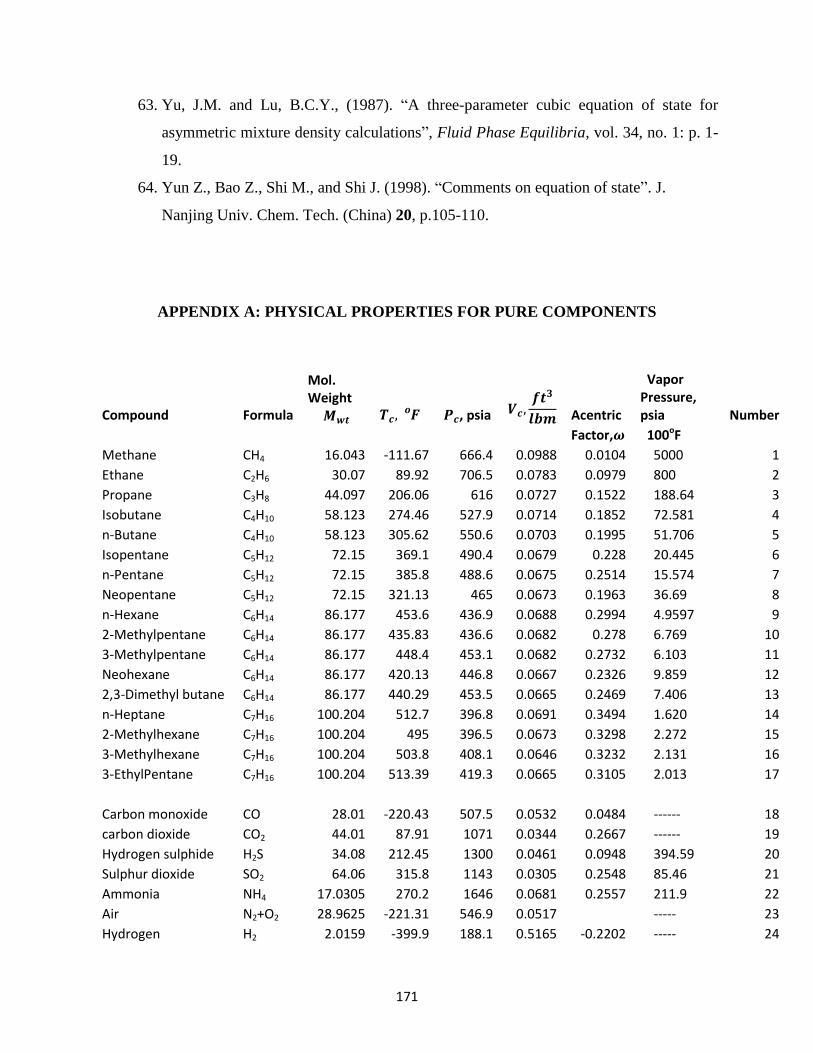
171
63. Yu, J.M. and Lu, B.C.Y., (1987). “A three-parameter cubic equation of state for
asymmetric mixture density calculations”, Fluid Phase Equilibria, vol. 34, no. 1: p. 1-
19.
64. Yun Z., Bao Z., Shi M., and Shi J. (1998). “Comments on equation of state”. J.
Nanjing Univ. Chem. Tech. (China) 20, p.105-110.
APPENDIX A: PHYSICAL PROPERTIES FOR PURE COMPONENTS
Compound Formula
Mol. Weight
𝑴𝒘𝒕 𝑻𝒄, 𝑭𝒐
𝑷𝒄, psia
𝑽𝒄,𝒇𝒕𝟑
𝒍𝒃𝒎 Acentric
Vapor Pressure, psia Number
Factor,𝝎 100oF
Methane CH4 16.043 -111.67 666.4 0.0988 0.0104 5000 1
Ethane C2H6 30.07 89.92 706.5 0.0783 0.0979 800 2
Propane C3H8 44.097 206.06 616 0.0727 0.1522 188.64 3
Isobutane C4H10 58.123 274.46 527.9 0.0714 0.1852 72.581 4
n-Butane C4H10 58.123 305.62 550.6 0.0703 0.1995 51.706 5
Isopentane C5H12 72.15 369.1 490.4 0.0679 0.228 20.445 6
n-Pentane C5H12 72.15 385.8 488.6 0.0675 0.2514 15.574 7
Neopentane C5H12 72.15 321.13 465 0.0673 0.1963 36.69 8
n-Hexane C6H14 86.177 453.6 436.9 0.0688 0.2994 4.9597 9
2-Methylpentane C6H14 86.177 435.83 436.6 0.0682 0.278 6.769 10
3-Methylpentane C6H14 86.177 448.4 453.1 0.0682 0.2732 6.103 11
Neohexane C6H14 86.177 420.13 446.8 0.0667 0.2326 9.859 12
2,3-Dimethyl butane C6H14 86.177 440.29 453.5 0.0665 0.2469 7.406 13
n-Heptane C7H16 100.204 512.7 396.8 0.0691 0.3494 1.620 14
2-Methylhexane C7H16 100.204 495 396.5 0.0673 0.3298 2.272 15
3-Methylhexane C7H16 100.204 503.8 408.1 0.0646 0.3232 2.131 16
3-EthylPentane C7H16 100.204 513.39 419.3 0.0665 0.3105 2.013 17
Carbon monoxide CO 28.01 -220.43 507.5 0.0532 0.0484 ------ 18
carbon dioxide CO2 44.01 87.91 1071 0.0344 0.2667 ------ 19
Hydrogen sulphide H2S 34.08 212.45 1300 0.0461 0.0948 394.59 20
Sulphur dioxide SO2 64.06 315.8 1143 0.0305 0.2548 85.46 21
Ammonia NH4 17.0305 270.2 1646 0.0681 0.2557 211.9 22
Air N2+O2 28.9625 -221.31 546.9 0.0517
----- 23
Hydrogen H2 2.0159 -399.9 188.1 0.5165 -0.2202 ----- 24

172
Oxygen O2 31.9988 -181.43 731.4 0.0367 0.0216 ----- 25
Nitrogen N2 28.0134 -232.51 493.1 0.051 0.0372 ----- 26
Water H2O 18.0153 705.16 3198.8 0.049 0.3443 157.3 27
APPENDIX B: FLOW CHART FOR CALCULATING Z-FACTOR
START
READ IN CONSTANT TERMS: Number of Components, 𝑛𝑐, 𝜋 = 22 7⁄ , 𝑅, 𝑇𝑒𝑚𝑝. ( 𝐹𝑜 ), 𝑃𝑟𝑒𝑠𝑠𝑢𝑟𝑒 (𝑃𝑠𝑖𝑎), 𝐶𝑟𝑖𝑡𝑖𝑐𝑎𝑙 𝑝𝑟𝑜𝑝𝑒𝑟𝑡𝑖𝑒𝑠
(𝑃𝑐𝑖𝑎𝑛𝑑 𝑇𝑐𝑖
), 𝑎𝑐𝑒𝑛𝑡𝑟𝑖𝑐 𝑓𝑎𝑐𝑡𝑜𝑟𝑠 (𝜔𝑖),Component mole fractions(𝑍𝑖′𝑠) and
molecular weights (𝑀𝑊𝑡𝑖′𝑠), 𝛺𝑎𝑎𝑛𝑑 𝛺𝑏
CONVERT TEMPERATURE UNITS: (fluid temperature and 𝑇𝑐𝑖) to
Absolute temperature in Rankine: (𝑇 ( 𝑅𝑜 ) = 𝑇( 𝐹𝑜 ) + 459.67)
CARRY OUT FLASH CALCULATIONS:
(1) Using Wilson’s Correlation obtain equilibrium Constants, (𝐾𝑖′𝑠):
𝑲𝒊 =𝟏
𝑷𝒓𝒊𝑬𝑿𝑷 [𝟓. 𝟑𝟕(𝟏 + 𝝎𝒊) (𝟏 −
𝟏
𝑻𝒓𝒊)]
(2) Solve Rachford Rice’s Equation for fraction of gas to liquid, 𝜶𝒈 at
equilibrium: ∑𝒁𝒊
𝟏+𝜶𝒈(𝑲𝒊−𝟏)
𝒏𝒄𝒊=𝟏 = 𝟏
(3) Solve for mole fraction of components in the liquid phase: 𝒙𝒊 =𝒛𝒊
𝟏+𝜶𝒈(𝑲𝒊−𝟏).
(4) Solve for mole fraction of components in the gas phase: 𝒚𝒊 = 𝒙𝒊𝑲𝒊.
1

173
1
CALCULATE REDUCED T & P AND EOS PARAMETERS PER COMPONENT:
𝑷𝒓𝒊=
𝑷
𝑷𝒄𝒊
, 𝑻𝒓𝒊=
𝑻
𝑻𝒄𝒊
, 𝒂𝒄𝒊= 𝜴𝒂 ∗ (𝑹𝟐 ∗ 𝑻𝒄𝒊
𝟐 𝑷𝒄𝒊⁄ ), 𝒃𝒊 = 𝜴𝒃 ∗ (𝑹 ∗ 𝑻𝒄𝒊
𝑷𝒄𝒊⁄ )
CALCULATE APPARENT MOLECULAR WEIGHT FOR GAS AND LIQUID PHASES:
FOR GAS PHASE: 𝑴𝑾𝒕𝒈 = ∑ 𝒚𝒊 ∗ 𝑴𝑾𝒕𝒊𝒏𝒄𝒊=𝟏
FOR LIQUID PHASE: 𝑴𝑾𝒕𝒍 = ∑ 𝒙𝒊 ∗ 𝑴𝑾𝒕𝒊𝒏𝒄𝒊=𝟏
𝑰𝑺 𝝎𝒊 ≤ 𝟎. 𝟒𝟗?
YES NO
𝒎𝒊 = 𝟎. 𝟑𝟕𝟗𝟔𝟒 + 𝟏. 𝟒𝟖𝟓𝟎𝟑𝝎𝒊 −
𝟎. 𝟏𝟔𝟒𝟒𝟐𝟑𝝎𝒊𝟐 + 𝟎. 𝟎𝟏𝟔𝟔𝟔𝝎𝒊
𝟑
𝒎𝒊 = 𝟎. 𝟑𝟕𝟒𝟔𝟒 + 𝟏. 𝟓𝟒𝟐𝟐𝟔𝝎𝒊
−𝟎. 𝟐𝟔𝟗𝟗𝟐𝝎𝒊𝟐
CALCULATE: 𝜶(𝑻)𝒊 = 𝟏 + 𝒎𝒊 ∗ [𝟏 − (𝑻𝒓𝒊)
𝟎.𝟓]
𝟐
, 𝒂𝜶(𝑻)𝒊 = 𝒂𝒄𝒊∗ 𝜶(𝑻)𝒊 ,
𝒂 = ∑ ∑ 𝒔𝒊𝒏𝒄𝒋=𝟏
𝒏𝒄𝒊=𝟏 ∗ (𝒂𝜶(𝑻)𝒊 ∗ 𝒂𝜶(𝑻)𝒋 ∗∗ 𝟎. 𝟓) ∗ (𝟏 − 𝑩𝑰𝑪𝒊,𝒋)
𝒃 = 𝒔𝒊 ∗ 𝒃𝒊
NOTE: For Gas Phase: 𝑠𝑖 = 𝑦𝑖 and For Liquid Phase: 𝑠𝑖 = 𝑥𝑖
𝐵𝐼𝐶𝑖,𝑗 is binary interaction coefficient between components 𝑖 ad 𝑗 respectively.
2

174
2
TO SOLVE THE CUBIC EQUATION:
𝒁𝟑 − (𝟏 − 𝑩)𝒁𝟐 + (𝑨 − 𝟑𝑩𝟐 − 𝟐𝑩)𝒁 − (𝑨𝑩 − 𝑩𝟐 − 𝑩𝟑) = 𝟎
CALCULATE THE PARAMETERS A AND B:
𝑨 = 𝒂 ∗ 𝑷 (𝑹𝑻)𝟐⁄ and 𝑩 = 𝒃𝑷 (𝑹𝑻)⁄
CALL SUBROUTINE TO SOLVE CUBIC IN Z EQUATION ANALYTICALLY
RETURN VALUES FOR 𝑍𝑚𝑎𝑥 , 𝑍𝑚𝑖𝑛𝑜𝑟 𝑠𝑖𝑛𝑔𝑙𝑒 𝑍
FOR GAS PHASE: 𝒁 = 𝒁𝒎𝒂𝒙,
FOR LIQUID PHASE: 𝒁 = 𝒁𝒎𝒊𝒏
STOP

VITA
PRINCESS C. NWANKWO
Born on July 22nd
1972 in Glasgow, United Kingdom.
EDUCATION
08/06 – 12/14 PhD in Petroleum and Natural Gas Engineering
Pennsylvania State University
07/00 – 12/04 M.Sc. Petroleum Engineering
University of Ibadan, Ibadan. Nigeria
08/98 – 09/00 Post Graduate Diploma in Petroleum Engineering
University of Benin, Benin City. Nigeria
07/86 – 11/91 B.Sc. Pure & Industrial Chemistry
University of Nigeria, Nsukka. Nigeria
EXPERIENCE
10/00 – 11/01 Personal Assistant to Professor of Petroleum Engineering and Chair
SHELL Petroleum Development Corporation,
University of Ibadan, Ibadan. Nigeria
01/01-08/03 Teaching and Research Assisstant, Department of Petroleum Engineering
University of Ibadan, Ibadan. Nigeria.
04/16 – 10/14 Faculty Member, Lecturer II,
Department of Petroleum Engineering,
University of Ibadan, Ibadan. Nigeria.
HONORS AND AWARDS
08/06 – 08/10 Faculty For The Future (FFTF) Award from
Schlumberger International at Penn State University, USA.