A New Look at Evaluating Fill TimesFor Injection Molding

Injection molding process methodologies

have evolved over the decades from a seat

of-the-pants black art to a more structured

approach. A number of schools, companies, and individuals pro-vide a valuable service to the industry by teaching these structured methods, which have been labeled with terms such as Scientific Molding, Decoupled Molding, and 2-Stage and 3-Stage processes. These approaches involve similar specific procedures that help establish a foundation on which to build a process. Among the procedures taught are a method for determining a fill time or fill speed using in-mold rheology curves (a.k.a “relative viscosity vs. relative shear rate” curves), as well as methods for establishing an ideal transfer position, ensuring the proper melt temperature, find-ing the ideal hold pressure, identifying pressure losses within the mold, and finding the time when gate seal (gate freeze) occurs. These approaches also teach that the process must be doc-umented in a manner that allows it to be transferred to other molding machines with the intent of achieving relatively consistent part quality. This requires that the process is recorded by referenc-ing plastic variables, not machine variables, and is done using a “universal setup sheet” (a term used by John Bozzelli, scientific-molding.com). For example, if you are documenting the melt temperature you would document the temperature of the plastic coming out of the machine nozzle—not the barrel temperature settings on the machine controller.

ESTABLISHING OPTIMUM FILL TIMEOne of the important process parameters to establish and record for any injection molded part is its injection or fill time. Fill time is an indication of how fast the plastic is injected into the mold. Fill time affects how much shear heating and shear thinning the plastic experiences, which in turn affect the material’s viscosity, the pressure and temperature of the plastic inside the cavities, and the overall part quality (dimensions, aesthetics, strength, etc.). Any change in fill timemay adversely affect the final molded part. Therefore once the ideal fill time is established for a given mold, that fill time should live with the mold forever and should be allowed to vary only slightly (±0.04 sec, as per John Bozzelli’s recommendation). The key question is: How does one go about identifying an ideal fill time for a given mold?

By David Hoffman & John Beaumont,Beaumont Technologies, Inc.

cover story

2 | AUGUST 2013 | PLASTICS TECHNOLOGY22 august 2013 Plastics technology

cover story

By David Hoffman & John Beaumont, Beaumont Technologies, Inc.

injection molding process methodologies

have evolved over the decades from a seat-

of-the-pants black art to a more structured

approach. A number of schools, companies, and individuals

provide a valuable service to the industry by teaching these

structured methods, which have been labeled with terms such as

Scientifc Molding, Decoupled Molding, and 2-Stage and

3-Stage processes. These approaches involve similar specifc

procedures that help establish a foundation on which to build a

process. Among the procedures taught are a method for deter-

mining a fll time or fll speed using in-mold rheology curves

(a.k.a “relative viscosity vs. relative shear rate” curves), as well

as methods for establishing an ideal transfer position, ensuring

the proper melt temperature, fnding the ideal hold pressure,

identifying pressure losses within the mold, and fnding the time

when gate seal (gate freeze) occurs.

These approaches also teach that the process must be docu-

mented in a manner that allows it to be transferred to other

molding machines with the intent of achieving relatively consis-

tent part quality. This requires that the process is recorded by

referencing plastic variables, not machine variables, and is done

using a “universal setup sheet” (a term used by John Bozzelli,

scientifcmolding.com). For example, if you are documenting

the melt temperature you would document the temperature of

the plastic coming out of the machine nozzle—not the barrel

temperature settings on the machine controller.

ESTABLISHING OPTIMUM FILL TIME

One of the important process parameters to establish and

record for any injection molded part is its injection or fll

time. Fill time is an indication of how fast the plastic is in-

jected into the mold. Fill time affects how much shear heating

and shear thinning the plastic experiences, which in turn

affect the material’s viscosity, the pressure and temperature of

the plastic inside the cavities, and the overall part quality

(dimensions, aesthetics, strength, etc.). Any change in fll time

may adversely affect the fnal molded part. Therefore once the

ideal fll time is established for a given mold, that fll time

should live with the mold forever and should be allowed to

vary only slightly (±0.04 sec, as per John Bozzelli’s recom-

mendation). The key question is: How does one go about

identifying an ideal fll time for a given mold?

Fig. 1 Relative viscosity vs. sheaR Rate

Re

lative

Vis

co

sit

yshear Rate

300,000

250,000

200,000

150,000

100,000

50,000

0

0.00 0.50 1.00 1.50 2.00 2.50 3.00 3.50 4.00 4.50

0.09

0.16

0.29

0.68 1.47 2.17 3.23 3.70 3.850.49

Fig. 2a sheaR Rate vs. viscosity cuRve

Vis

co

sit

y, p

ols

e

shear Rate, 1/s

10000

1000

100

10

1

1 10 100 1000 10000 100000

Fig. 2B sheaR Rate vs. viscosity cuRve

Vis

co

sit

y, p

ols

e

shear Rate, 1/s

6000

5000

4000

3000

2000

1000

0

0 20000 40000 60000 80000 100000

a new look at evaluating Fill timesFor injection Molding

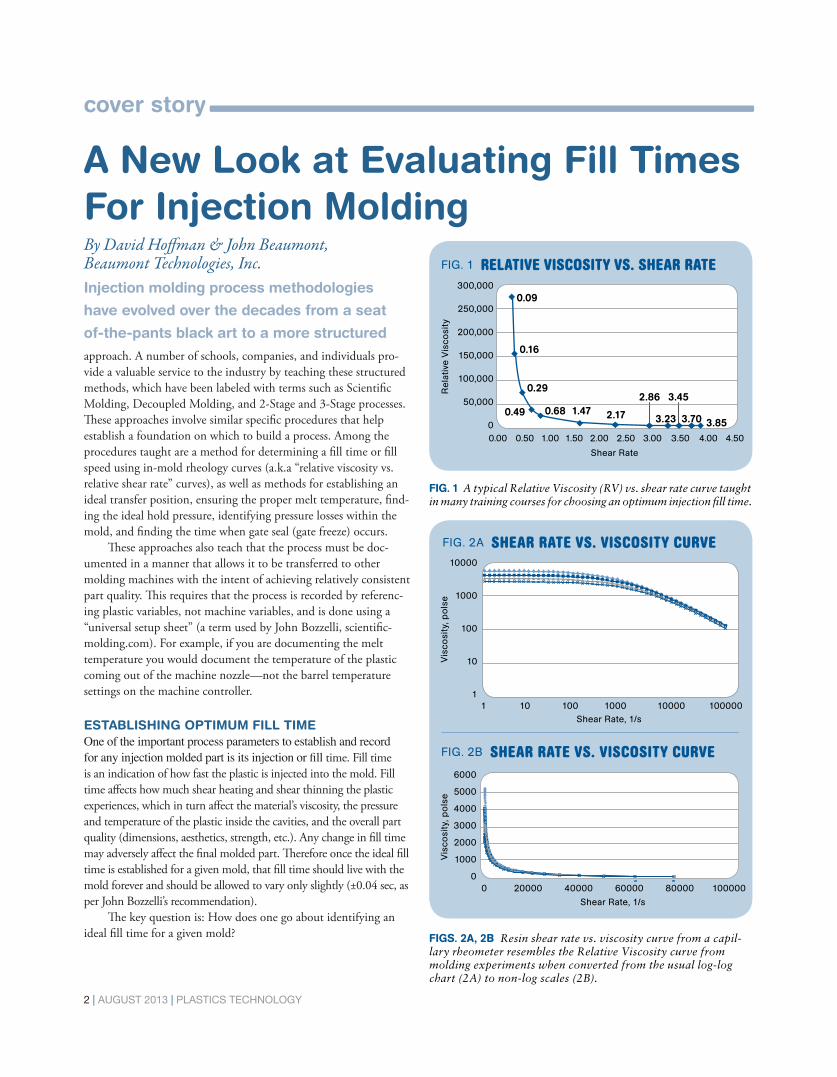
FIG. 1 A typical Relative Viscosity (RV) vs. shear rate curve taught in many training courses for choosing an optimum injection fll time.

FIGS. 2A, 2B Resin shear rate vs. viscosity curve from a capil-lary rheometer resembles the Relative Viscosity curve from molding experiments when converted from the usual log-log chart (2A) to non-log scales (2B).

2.86 3.45

Molders use several methods to establish a fill time, some of which begin with one of the following methods:

• Evaluating the fill time used on similar parts and molds. • Trial and error. • Design of experiments (DOE) data. • Experience. • Mold-filling simulation. • Relative Viscosity test.

Ideally, every part would be evaluated for fill time using moldfilling simulation performed by a skilled analyst with plastics processing experience. Unfortunately this type of analysis data is not available for many plastic parts, so molders need a method to establish an ideal fill time that they can employ on the shop floor. This is where the Relative Viscosity (RV) test comes into play. The general procedure for this commonly taught method is presented below. Though some consultants and trainers may add other steps or teach it a bit differently, essentially the approaches are very similar:

1. Using maximum injection velocity, adjust shot size to get the fullest part 95% full. 2. Record the fill time and pressure at transfer. 3. Reduce injection velocity and record the fill time and pressure at transfer. 4. Repeat Step 3 until the fill time is over 10 sec. 5. Use the data to calculate relative shear rates and relative viscosities: Relative Shear Rate = 1 ÷ fill time Relative Viscosity = Hydraulic pressure x intensification ratio x fill time 6. Graph relative viscosity (y-axis) vs. relative shear rate (x-axis). 7. Select a fill time on the “flat” portion of the curve.

The results of one RV test are shown graphically in Fig. 1.Note that the graph is essentially that of “Fill Time vs. 1 ÷ FillTime” (where the Fill Time on the y-axis is multiplied by itscorresponding pressure). When you graph a number versus itsreciprocal, the shape of the curve shown in Fig. 1 is expected. Ifthe change in pressure were directly proportional to the changein fill time, the graph would show a straight line. However, thistest demonstrates that as plastic flows faster (higher shear rate),its viscosity is reduced and becomes fairly consistent over a widerange of injection rates. The RV test results in “viscosity vs. shear rate” curves thatlook similar to those produced using laboratory capillary rheome-ters (Figs. 2A, 2B). Figure 2A shows the capillary rheometerdata of viscosity (poise) versus shear rate (1/sec) plotted on alog-log graph while Fig. 2B shows the same data plotted on anon-log-log graph. The non-log-log graph in Fig. 2B looks verysimilar to the RV graph in Fig. 1. The RV test has been widely taught and adopted by manymolding companies to help select a fill time for a given mold.Company procedures have been written to include the test aspart of their process standards. Thus, there is a great deal of

injection fill time

AUGUST 2013 | PLASTICS TECHNOLOGY | 3 Plastics technology august 2013 23

injection fll time

Fig. 3a master graph0.1 seconds - 20 seconds

Fill tim

e

Relative shear Rate

22.5

20

17.5

15

12.5

10

7.5

5

2.5

00.00 2.00 4.00 6.00 8.00 10.00 12.00

Fig. 3b master graph truncated0.3 seconds - 5 seconds

Fill tim

e

Relative shear Rate

7.5

5

2.5

0

0.00 0.50 1.00 1.50 2.00 2.50 3.00 3.50

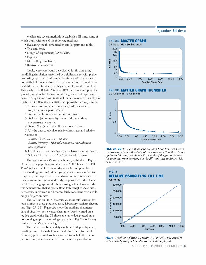
FIGS. 3A, 3B One problem with the shop-foor Relative Viscos-ity procedure is that the shape of the curve, and thus the selected optimum fll time, can change if the scale of the graph changes—for example, from carrying out the fll-time tests to 20 sec (3A) or to 5 sec (3B).

FIG. 4 Graph of Relative Viscosity (RV) vs. Fill Time appears to be a nearly straight line, due to the scale employed.

Molders use several methods to establish a fll time, some of

which begin with one of the following methods:

•Evaluating the fll time used on similar parts and molds.

•Trial and error.

•Design of experiments (DOE) data.

•Experience.

•Mold-flling simulation.

•Relative Viscosity test.

Ideally, every part would be evaluated for fll time using mold-

flling simulation performed by a skilled analyst with plastics pro-

cessing experience. Unfortunately this type of analysis data is not

available for many plastic parts, so molders need a method to estab-

lish an ideal fll time that they can employ on the shop foor. This is

where the Relative Viscosity (RV) test comes into play. The general

procedure for this commonly taught method is presented below.

Though some consultants and trainers may add other steps or teach

it a bit differently, essentially the approaches are very similar:

1. Using maximum injection velocity, adjust shot size to get

the fullest part 95% full.

2. Record the fll time and pressure at transfer.

3. Reduce injection velocity and record the fll time and

pressure at transfer.

4. Repeat Step 3 until the fll time is over 10 sec.

5. Use the data to calculate relative shear rates and relative

viscosities:

Relative Shear Rate = 1 ÷ fll time

Relative Viscosity = Hydraulic pressure x intensifcation

ratio x fll time

6. Graph relative viscosity (y-axis) vs. relative shear rate (x-axis).

7. Select a fll time on the “fat” portion of the curve.

The results of one RV test are shown graphically in Fig. 1.

Note that the graph is essentially that of “Fill Time vs. 1 ÷ Fill

Time” (where the Fill Time on the y-axis is multiplied by its

corresponding pressure). When you graph a number versus its

reciprocal, the shape of the curve shown in Fig. 1 is expected. If

the change in pressure were directly proportional to the change

in fll time, the graph would show a straight line. However, this

test demonstrates that as plastic fows faster (higher shear rate),

its viscosity is reduced and becomes fairly consistent over a wide

range of injection rates.

The RV test results in “viscosity vs. shear rate” curves that

look similar to those produced using laboratory capillary rheom-

eters (Figs. 2A, 2B). Figure 2A shows the capillary rheometer

data of viscosity (poise) versus shear rate (1/sec) plotted on a

log-log graph while Fig. 2B shows the same data plotted on a

non-log-log graph. The non-log-log graph in Fig. 2B looks very

similar to the RV graph in Fig. 1.

The RV test has been widely taught and adopted by many

molding companies to help select a fll time for a given mold.

Company procedures have been written to include the test as

part of their process standards. Thus, there is a great deal of

material, labor, and machine time spent each day on running the

RV tests in hopes of identifying optimum fll times based on a

Fig. 4

relative viscosity vs. fill timeall Points

Rela

tive

Vis

co

sit

y

Fill time

300,000

250,000

200,000

150,000

100,000

50,000

00.00 2.00 4.00 6.00 8.00 10.00 12.00

material, labor, and machine time spent each day on running theRV tests in hopes of identifying optimum fill times based on a structured approach that a process technician or engineer canuse on the shop floor. Ideally, someone applying this technique should also be evaluating the parts for cosmetic issues and other defects to help determine the optimum fill time. But all too often we have found molders looking at the curves as a scientifically founded method to establish optimum fill time and therefore assuming they shouldlook at other process parameters to address molded part problems. Those who teach the RV test method usually state that formost parts the fill time should be located somewhere on theflatter portion of the curve (after the “elbow”). The flat portionof the curve is considered desirable because it is expected toproduce the most consistent melt conditions when changes occurin the process or resin viscosity. These changes might result fromlot-to-lot material variations or process drift. Depending on the range of fill times used, the flat portion ofthe curve can be a small area or rather large. This leaves theprocessor asking, “Where on the flat portion of the RV curve isthe optimum fill time?” Currently the practice of picking the filltime from the curve is quite arbitrary. If you ask three differentmolders taught in the same class to select a fill time from thesame RV graph you may get three different answers. Listedbelow are several common opinions and one formula that havebeen suggested as guidelines for selecting the target fill time:

Method 1: Halfway from the “knee” to the end of the curve.Method 2: The point right after the “knee.”Method 3: The farthest point out, because it has the lowestviscosity overall.Method 4: ([(Highest RV – Lowest RV) x 0.05] ÷ 2) + Lowest RV A further complication is that the selected fill time is com-pletely dependent on the scale of the graph at hand. If the scaleof the graph changes (i.e. run the test to only 5 sec instead of 10or 20 sec), the fill time chosen by using the current visual andarbitrary fill-time selection methods may actually change (Fig.3A vs. 3B). Also, the ideal fill time may be harder to determinesince the flat part of the curve will not look as flat as it doeswhen running the test with more data points at longer fill times.In addition to some ambiguity in the interpretation of the RVtest, the method of focusing on a “relative viscosity” to identifya fill time raises further questions. It was apparent that furtherresearch was required to better understand the RV test anddetermine if it could be improved upon. This research beganseveral years ago and only a portion is reported here.

RESEARCHING THE FILL-TIME PROBLEMEarly stages of this work began with us asking ourselves, “What do relative viscosity and relative shear rate really mean?” The relative shear rate is defined as 1 ÷ fill time, which methresults in units of 1/sec, the same units used by rheologists for describing shear rates.

However actual shear rate depends on the volumetric flow rate, the non-Newtonian characteristics (n), and the specific geometry through which the plastic is flowing, as per the following equation:

4 | AUGUST 2013 | PLASTICS TECHNOLOGY24 august 2013 Plastics technology

structured approach that a process technician or engineer can

use on the shop foor.

Ideally, someone applying this technique should also be evalu-

ating the parts for cosmetic issues and other defects to help deter-

mine the optimum fll time. But all too often we have found mold-

ers looking at the curves as a scientifcally founded method to

establish optimum fll time and therefore assuming they should

look at other process parameters to address molded part problems.

Those who teach the RV test method usually state that for

most parts the fll time should be located somewhere on the

fatter portion of the curve (after the “elbow”). The fat portion

of the curve is considered desirable because it is expected to

produce the most consistent melt conditions when changes occur

in the process or resin viscosity. These changes might result from

lot-to-lot material variations or process drift.

Depending on the range of fll times used, the fat portion of

the curve can be a small area or rather large. This leaves the

processor asking, “Where on the fat portion of the RV curve is

the optimum fll time?” Currently the practice of picking the fll

time from the curve is quite arbitrary. If you ask three different

molders taught in the same class to select a fll time from the

same RV graph you may get three different answers. Listed

below are several common opinions and one formula that have

been suggested as guidelines for selecting the target fll time:

FIG. 5 Fill times from the novel 2 Point Rheology Curve were used to calculate Relative Viscosity and Relative Shear Rate, producing an RV curve nearly identical to the RV curve gener-ated from 12 molding data points. The ability of two fll-time data points to generate the same curves as 12 fll-time points was found to be true for a variety of molds and materials.

Fig. 5 Relative viscosity vs. sheaR Rate2 points

Re

lative

Vis

so

sit

y

shear Rate

300,000

250,000

200,000

150,000

100,000

50,000

0

0.00 0.50 1.00 1.50 2.00 2.50 3.00 3.50 4.00 4.50

actual RV Data

calculated RV

© Copyright 2013 Novatec, Inc.

• Exclusiveinternallifetimemembranetechnologyneverrequiresdesiccant!

• Patenteddesignconsumes70%lesscompressedairthanothers

• Dewpointcontrolassures-40˚dewpointperformance

• Instockforimmediateshipment!

800-237-8379 | www.novatec.com

The term relative shear rate differs from actual shear rate in anumber of ways. One is that there is no geometry considerationin the relative shear-rate calculation. In actuality, the flow geome-try of a mold is constantly changing (nozzle, sprue, progressiverunner branches, gates, and cavity). The actual shear rate thereforevaries considerably in a mold and can range from a few hundred 1/sec in a cavity to hundreds of thousands in a gate. During our research we found that when graphing typicalRV data vs. Fill time (FT), a nearly straight line developed (Fig. 4). Surely it cannot really be a pure straight line, due to the pseu-do-plastic, non-Newtonian behavior of plastics; but the scale at which we are working with causes this to appear linear. From this phenomenon we theorized that we could very closely recreate the original RV curve by utilizing only two data points. This method-ology will be referred to as a “2 Point Rheology Curve.”

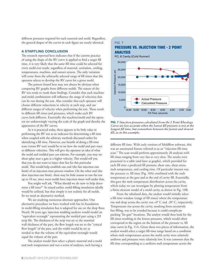
Utilizing the data from Fig. 4, we selected two random data points. Then we selected a starting (fastest) fill time equal tothat of the original mold and increased the fill time by 25% until the ending (slowest) fill time was near that of the original mold.Relative Viscosity and Relative Shear Rate were then back-calculat-ed for the fill times. The result was an RV curve, created usingonly two data points, that was nearly identical to the original RV curve generated from 12 data points (Fig. 5). Using the same approach, 2 Point Rheology Curves were then created for more than 40 other randomly selected production molds. These molds ranged from one to 32 cavities; used differentmelt-delivery systems (hot runner, hot-to-cold runner, and full cold runner); and were run with different plastic materials(such as PP, PC, and glass-filled PBT, PCT, and nylon 66). In each case, the 2 Point Rheology Curve very closely mimicked the original RV curve, similar to Fig. 5. We theorized that the injection pressure might also be back-calculated for any fill time using the 2 Point Rheology Curve methodology. It was found that this method was within very reasonable limits of calculating fill pressure vs. actual pressurein most cases, regardless of differing cavitation, melt-delivery sys-tem, or plastic material. The method was found to providea good prediction of mold filling pressures in molds where the pressure continually increased with decreasing fill time (Fig. 6 is one example). In contrast, the method worked poorly in predicting pressures when the lowest fill pressure was not at the slowest fill time, but rather somewhere between the slowest and fastest fill time (Fig. 7). Regardless of the pressure prediction, the calculated RV curves looked nearly identical to the original curves. Next, the plots of the original RV data for the same molds were compared with plots of random fill times versus relativeshear rate (1/FT) over the same range of fill times used in the actu-al RV test. It was noticed that the resulting two curves looked very similar, though the slopes between data points were different due to the influence of pressure on the y-axis values (Fig. 8A). When the curves were plotted separately and shifted to overlay on top of one another, the two curves overlaid very well (Fig. 8B). This indicates that by using the arbitrary methods of selecting a fill time on a RV curve, it would be nearly impossible to explain why you would pick a different fill time on the original RV curve vs. one from the Random Fill Time curve. It must be understood that the Random Fill Time Curve data does not include any influence of pressure or material or mold-ing of actual parts. The curve was created by plotting time steps between the fastest and slowest fill times of the original RV data versus the reciprocals of those time steps. But yet the Random Fill Time curve is nearly identical to the actual RV curve. These find-ings were consistent over all molds tested and are a result of sound mathematical equations and substitutions.The results prove that any RV curve can be made to look nearly identical to any other simply by adjusting the vertical scales.

AUGUST 2013 | PLASTICS TECHNOLOGY | 5Plastics technology august 2013 25

Fig. 6 pressure Vs. injection time -

2 point analysis

15% gF PBt; 4 cavity (2 Drop hot-to-cold Runner system)

inje

ctio

n P

ressure

, p

si

Fill time, seconds

FIG. 6 Back-calculating injection pressure from the 2 Point Rheology Curve gives results very close to the actual pressure in most cases where fll pressure increases with decreasing fll time.

Method 1: Halfway from the “knee” to the end of the curve.

Method 2: The point right after the “knee.”

Method 3: The farthest point out, because it has the lowest

viscosity overall.

Method 4: ([(Highest RV – Lowest RV) x 0.05] ÷ 2) + Lowest RV

A further complication is that the selected fll time is com-

pletely dependent on the scale of the graph at hand. If the scale

of the graph changes (i.e. run the test to only 5 sec instead of 10

or 20 sec), the fll time chosen by using the current visual and

arbitrary fll-time selection methods may actually change (Fig.

3A vs. 3B). Also, the ideal fll time may be harder to determine

since the fat part of the curve will not look as fat as it does

when running the test with more data points at longer fll times.

In addition to some ambiguity in the interpretation of the RV

test, the method of focusing on a “relative viscosity” to identify

a fll time raises further questions. It was apparent that further

research was required to better understand the RV test and

determine if it could be improved upon. This research began

several years ago and only a portion is reported here.

RESEARCHING THE FILL-TIME PROBLEM

Early stages of this work began with us asking ourselves,

“What do relative viscosity and relative shear rate really

mean?” The relative shear rate is defned as 1 ÷ fll time, which

BI-POWERPowerful Compact Reliable Precise Accurate

The Answer Is Technology | Innovation | Effciency

NEGRI BOSSI NA 311 Carroll Drive, Building 100 | New Castle, DE 19720 | Tel: (302) 328-8020 | sales@negribossiusa.com | www.negribossiusa.com

The BI-POWER from Negri Bossi offers peak performance and reliability – all packed into a compact footprint – thanks to a robust two-platen design incorporating a dual cylinder injection assembly. The standard electric screw drive offers process effciency and reduced cycle times. Available in eight models ranging from 1050 to 7700 tons.

T W OPLATEN

Robust and reliable low-profle with a compact footprint

Unsurpassed clamp open / close / lock-up speeds

Oversized moving platen support for large molds

Bi-metallic barrel and ceramic heater bands standard

Electric screw drive with parallel axis gear reduction

20,000

18,000

16,000

14,000

12,000

10,000

8,000

6,000

4,000

2,000

0

actual Pressure

calculated Pressure

2.50 2.00 1.50 1.00 0.50 0.00

Based on these findings and the nature of the RV test itself, we theorized that every mold would produce the same general RV curve, given the same fill times. This would indicate that every mold would have the same selected fill time according to current practices of the RV method. To test this theory, an RV test was run on an eight-cavity test mold using an acetal resin. The test was performed by strategically changing the machine velocity settings to match the fill times (as closely as possible) to four of the previously tested molds plus the same eight-cavity mold using a PC resin. Thus, five different RV curves were generated for the same eightcavity mold. Matching the same fill times as the previously tested molds allowed us to main-tain the same scale for the Relative Shear Rate x-axis. The data was then overlaid on top of the graph of the original RV data for each of the five molds. When molding acetal in the eight-cavity test mold, it was found that by matching fill times to those of the original molds,each original RV curve and its corresponding eight-cavity acetal test-mold RV curve looked nearly identical to one another. Asan example, Fig. 9 shows the fill times for each mold along with overlaid graphs of the original mold’s RV curve (red) and theeight-cavity acetal RV curve (blue). The x and y-axis labels are removed for clarity reasons but correspond to Relative Shear Rate and Relative Viscosity respectively. The x-axes are lined up to one another as a result of the corresponding fill times, but as discussed earlier, a shift up/down was required to get the graphs to overlay due to the different slopes between data points resulting from the

different pressures required for each material and mold. Regardless, the general shapes of the curves in each figure are nearly identical.

A STARTLING CONCLUSIONThe research reported here indicates that if the current practice of using the shape of the RV curve is applied to find a target fill time, it is very likely that the same fill time could be selected for every mold ever made, regardless of material, cavitation, cooling, temperatures, machine, and runner system. The only variation will come from the arbitrarily selected range of fill times that the operator selects to develop the RV curve for a given mold. The pattern found here may not always be obvious whencomparing RV graphs from different molds. The nature of theRV test tends to mask these findings. Consider that each machineand mold combination will influence the range of velocities that can be run during the test. Also consider that each operator will choose different reductions in velocity at each step, and usedifferent ranges of velocity when performing the test. These result in different fill times and pressures, which make each RVcurve look different. Essentially the machine/mold and the opera-tor are unknowingly varying the scale of the graph and thereby the appearance of the RV curves. As it is practiced today, there appears to be little value in performing the RV test as an indicator for determining a fill timewhen coupled with the arbitrary methods discussed earlier for identifying a fill time. However, one benefit of doing a fill-timescan (versus RV test) would be to see how the mold and part react to different velocities. This will give the operator an idea of what the mold and molded part can tolerate. For example, you may seeshear splay near a gate at a higher velocity. This would tell you that you do not want to inject that fast for this particularmold. This would help establish one end (the fast injection-rate limit) of an injection-time process window. On the other end (the slow injection-rate limit), there may be little reason to run the test up to 10 sec, since most molds have injection times well under that. You might well ask, “What should we do now to help deter-mine a fill time?” As stated earlier, mold-filling simulation ideally would be utilized, but that simply is not realistic for all molds. So we need an alternative method. We are studying numerous alternate approaches. One alternative procedure we have worked with has its foundation in mold-filling simulation but is adapted for use on the shop floor. Nearly 30 years ago, injection molding analysts would model an “equivalent rectangle” representing the molded part using a 2Dstrip file. The thickness of the strip was set to the nominalwall thickness of the part, the flow length was set to the “criticalflow length” of the part, and the width would be set asneeded so that the volume of the equivalent rectangle wouldequal the volume of the part. The analyst would then select a plastic material and a moldand melt temperature and run a series of analyses, each having a

different fill time. With early versions of Moldflow software, thiswas an automated feature referred to as an “injection fill-timescan.” The scan would perform approximately 20 analyses withfill times ranging from very fast to very slow. The results were presented in a table (and later as graphs), which provided for each fill time a predicted fill pressure, shear rate, shear stress, melt temperature, and cooling time. Of particular interest was the pressure vs. fill time (Fig. 10A) combined with the melt temperature at the gate and at the end of cavity fill. Essentially, this gave the melt-temperature distribution across the cavity, which today we can investigate by plotting temperature from a finite-element model of a mold cavity, as shown in Fig. 10B. From the tabulated data, the analyst would initially selecta fill-time window (range of fill times) where the temperaturerise and drop across the cavity was +0° C and -20° C, respectively.Temperature rise across the cavity, resulting from excessivelyfast filling, was to be avoided because it could complicatepacking “far gate” locations. The analyst would then look for the fill times resulting in the lowest pressures, which would often correspond to the region on the bottom of the pressure vs. fill time curve in Fig. 11A. Given these two pieces of information, the analyst would select a target fill-time range based on a condition where melt temperatures across the mold cavity were relatively uniform and pressures were relatively low. It was common that the fill time corresponding to a uniform melt temperature across the

6 | AUGUST 2013 | PLASTICS TECHNOLOGY26 august 2013 Plastics technology

Utilizing the data from Fig. 4, we se-

lected two random data points. Then we

selected a starting (fastest) fll time equal to

that of the original mold and increased the

fll time by 25% until the ending (slowest)

fll time was near that of the original mold.

Relative Viscosity and Relative Shear Rate

were then back-calculated for the fll times.

The result was an RV curve, created using

only two data points, that was nearly

identical to the original RV curve gener-

ated from 12 data points (Fig. 5).

Using the same approach, 2 Point

Rheology Curves were then created for

more than 40 other randomly selected

production molds. These molds ranged

from one to 32 cavities; used different

melt-delivery systems (hot runner, hot-to-

cold runner, and full cold runner); and

were run with different plastic materials

(such as PP, PC, and glass-flled PBT, PCT,

and nylon 66). In each case, the 2 Point

Rheology Curve very closely mimicked the

original RV curve, similar to Fig. 5.

We theorized that the injection pres-

sure might also be back-calculated for any

fll time using the 2 Point Rheology Curve

methodology. It was found that this meth-

results in units of 1/sec, the same units used by rheologists for

describing shear rates. However actual shear rate depends on

the volumetric fow rate, the non-Newtonian characteristics

(n), and the specifc geometry through which the plastic is

fowing, as per the following equation:

��

���

� +=

n

n

r

Q

4

134

3p

g

The term relative shear rate differs from actual shear rate in a

number of ways. One is that there is no geometry consideration

in the relative shear-rate calculation. In actuality, the fow geom-

etry of a mold is constantly changing (nozzle, sprue, progressive

runner branches, gates, and cavity). The actual shear rate there-

fore varies considerably in a mold and can range from a few

hundred 1/sec in a cavity to hundreds of thousands in a gate.

During our research we found that when graphing typical

RV data vs. Fill time (FT), a nearly straight line developed

(Fig. 4). Surely it cannot really be a pure straight line, due to

the pseudo-plastic, non-Newtonian behavior of plastics; but

the scale at which we are working with causes this to appear

linear. From this phenomenon we theorized that we could

very closely recreate the original RV curve by utilizing only

two data points. This methodology will be referred to as a “2

Point Rheology Curve.”

800-835-2526 www.buntingmagnetics.com©2013 Bunting® Magnetics Co.

Bunting Machine-Mounted All-Metal Separators

provide efficient rejection of both ferrous and

nonferrous metal contaminants and fit where

headroom is limited.

Superior ProtectionBunting products are the plastics industry standard for equipment protection

FF Series Drawer Magnets

Plastics industry’s most popular

choice for extrusion, injection and

blow molding equipment.

Parts Handling Move-It™ Conveyors

Built to order but priced like stock,

available in the most common conveyor

sizes and can be custom ordered in

a wide range of lengths and widths to

fit your application. (Six styles to choose from)

Fill time, secondsin

jectio

n P

ressure

, p

si

FIG. 7 Injection pressures calculated from the 2 Point Rheology Curve are less accurate when the lowest fll pressure is not at the longest fll time, but somewhere between the fastest and slowest fll, as in this example.

14.00 12.00 10.00 8.00 6.00 4.00 2.00 0.00

30,000

25,000

20,000

15,000

10,000

5,000

0

Fig. 7

Pressure Vs. injection time - 2 Point

AnAlysisPc; 8 cavity (cold Runner)

actual Pressure

calculated Pressure

cavity would be near to the lowest pressure. It was also considered desirable that the slow end of the target fill-time range be slightly faster than the time corresponding to the lowest pressure, as thiswould be a shear-dominated rather than thermally dominatedcavity condition. This method also has the advantage that itfocuses on the part-forming cavity condition, unlike the RVmethod. Countless molds have been processed with greatsuccess utilizing these older simulation techniques. The fundamentals of the injection-time scan method arequite sound and apply logical methodologies. The process isfocused on the quality of the molded part as influenced by themelt conditions within the mold cavity. The currently practicedRV test method is incapable of isolating and evaluating rheologicalconditions within the cavity. Additionally, the RV data isdetermined from a conglomeration that includes the energy tomove the screw and pressure loss through the machine’s end cap,nozzle, sprue, runner system, gate, and finally the cavity. Astable Relative Viscosity in the overall conglomeration does notnecessarily represent a stable viscosity within the mold cavity. Itis the conditions within the cavity that are most significant indetermining the outcome of the final molded part. Unfortunately there is no good technology currently availablefor the shop floor to determine the melt-temperature distributionacross the cavity. However all molding machines have the abilityto provide injection pressure vs. fill time data.

AUGUST 2013 | PLASTICS TECHNOLOGY | 7

Though only being able to evaluate Pressure vs. Fill Time has its limitations, it still can provide molders some valuable information to help them make more informed decisions. Since the user will be focused on the pressure changes instead of a Relative Viscosity number, this methodology will provide a quick indication of the fill time at which the process will be close to being pressure-limited. In addition, we find that “fill time” and “pressure” are terms that a processor is familiar with and are more easily interpreted than Relative Viscosity and RelativeShear Rate. And finally, there are no calculations required forthe Pressure versus Fill Time graph other than multiplying yourpressure by the machine’s intensification ratio, if needed (not inthe case of an electric machine). Processors, mold designers, and engineers can also be taughthow to calculate actual shear rates in selected mold regions. Astrue shear degradation limits are not well known or understoodin this industry, this practice can allow a company to establish adefect log per material and shear rate. This data can be useful toboth mold designers and processors. For example, a designercould increase a gate size if the log indicated that the currentgate-size and flow-rate combination produced a shear rate thathistorically caused shear splay for a given material. We continue to study this approach and teach this informa-tion in our continuing education and training courses, alongwith other methods that could be used to help the molder on

Plastics technology august 2013 27

FIGS. 8A, 8B Plots of RV data were compared with plots of random fll times versus relative shear rate (1/FT) over the same range of fll times used in the actual RV test for the same molds. The resulting two curves are very similar, though the

slopes between data points are different due to the infuence of pressure on the y-axis values (8A). But when the curves are shifted they overlay on top of one another very well (8B). This was consistent for all molds tested.

od was within very reasonable limits of

calculating fll pressure vs. actual pressure

in most cases, regardless of differing

cavitation, melt-delivery system, or plastic

material. The method was found to pro-

vide a good prediction of mold flling

pressures in molds where the pressure

continually increased with decreasing fll

time (Fig. 6 is one example).

In contrast, the method worked poorly

in predicting pressures when the lowest

fll pressure was not at the slowest fll

time, but rather somewhere between the

slowest and fastest fll time (Fig. 7). Re-

gardless of the pressure prediction, the

calculated RV curves looked nearly iden-

tical to the original curves.

Next, the plots of the original RV data

for the same molds were compared with

plots of random fll times versus relative

shear rate (1/FT) over the same range of

fll times used in the actual RV test. It was

noticed that the resulting two curves

looked very similar, though the slopes

between data points were different due to

the infuence of pressure on the y-axis

values (Fig. 8A). When the curves were

plotted separately and shifted to overlay

Fig. 8a

Random fill time & Relative viscosity

vs. Relative sheaR Rate15% gF PBt; 4 cavity (2 Drop hot to cold Runner system)

16,000

14,000

10,000

8,000

6,000

4,000

2,000

0

2.5

2

1.5

1

0.5

0

Relative shear Rate

Rela

tive

Vis

co

sit

y

Fig. 8B

Random fill time vs. Relative sheaR Rate

15% gF PBt; 4 cavity (2 Drop hot to cold Runner system)

actual RV Data

Random Fill time vs.

Relative shear Rate

0 1 2 3 4 5 6

2.5

2

1.5

1

0.5

0

16,000

14,000

12,000

10,000

8,000

6,000

4,000

2,000

0

Relative shear Rate

Fill t

ime

Rela

tive

Vis

co

sit

y

Fill t

ime

0 1 2 3 4 5 6

the shop floor to identify a preferred fill-time window. Thesemethods include consideration of both fast and relatively slow fill times. If you choose to use the RV method and feel it provides benefit, a great deal of time and money could be saved by adopting our 2 Point Rheology Curve presented here. This data wouldallow a molder to hone in on the “flat” part of the curve (if de-sired) much faster and at a reduced cost. A more recent method we are researching is the concept of a “critical velocity” based on the polymer melt, wall thickness, and flow length. The critical velocity is a condition where the ther-mal and shear conditions are at equilibrium, establishing relatively stable melt conditions, shear stresses, and frozen-layer thicknesses across the partforming cavity. This method uses our new Ther-ma-flo injection moldability characterization method (see June 2012 issue). The critical velocity would be a material characteriza-tion that could provide the optimum fill time for a mold prior to actually running the mold. No matter which method you choose for finding a fill time, it should be considered only a starting point. The molder should understand the limitations of these methods and adapt the process to achieve the design and application requirements of the actual molded part. This includes consideration of all required quality criteria, including cosmetics, dimensions, warpage, etc. And once the optimum fill time and process have been identified, be sure to document the process using a universal setup sheet.

ABOUT THE AUTHORSDavid Hoffman is the senior instructor and training development manager at Beaumont Technologies, Inc. in Erie, Pa., where he co-invented the MeltFlipper Multi-Axis rheological control technology. He is a 20- year industry veteran with experience in part design, processing, and mold design/manufacturing. Contact: (814) 899-6390; email: dhoffman@beaumontinc.com; web: beaumontinc.com.John Beaumont, president and CEO of Beaumont Technologies, is also professor and former chairman in the Plastics Engineering Technology program at PennState Erie. He founded the University’s Plastics CAE Center and authored several books, including the Runner and Gating Handbook and Successful Injection Molding.

MeltFlipper® | Continuing Education | Molding Simulation | p: (814) 899-6390 | www.Beaumontinc.com

Continuing EducationEducation is the resource to knowledge, higher-level thought & creativity. In the Injection Molding Industry, these values are the resource of invention, problem solving, increased productivity, quality & profit. Experience the Beaumont Difference.