algorithms

Article

A New Lossless DNA Compression AlgorithmBased on A Single-Block Encoding Scheme

Deloula Mansouri , Xiaohui Yuan * and Abdeldjalil Saidani

School of Computer Science and Technology, Wuhan University of Technology, Wuhan 430070, China;deloula@whut.edu.cn (D.M.); saidani@whut.edu.cn (A.S.)* Correspondence: yuanxiaohui@whut.edu.cn

Received: 24 March 2020; Accepted: 17 April 2020; Published: 20 April 2020�����������������

Abstract: With the emergent evolution in DNA sequencing technology, a massive amount of genomicdata is produced every day, mainly DNA sequences, craving for more storage and bandwidth.Unfortunately, managing, analyzing and specifically storing these large amounts of data becomea major scientific challenge for bioinformatics. Therefore, to overcome these challenges, compressionhas become necessary. In this paper, we describe a new reference-free DNA compressor abbreviatedas DNAC-SBE. DNAC-SBE is a lossless hybrid compressor that consists of three phases. First, startingfrom the largest base (Bi), the positions of each Bi are replaced with ones and the positions of otherbases that have smaller frequencies than Bi are replaced with zeros. Second, to encode the generatedstreams, we propose a new single-block encoding scheme (SEB) based on the exploitation of theposition of neighboring bits within the block using two different techniques. Finally, the proposedalgorithm dynamically assigns the shorter length code to each block. Results show that DNAC-SBEoutperforms state-of-the-art compressors and proves its efficiency in terms of special conditionsimposed on compressed data, storage space and data transfer rate regardless of the file format or thesize of the data.

Keywords: DNA sequence; storage; lossless compression; FASTA files; FASTQ files; binary encodingscheme; single-block encoding scheme; compression ratio

1. Introduction

Bioinformatics is a combination of the field of informatics and biology, in which computationaltools and approaches are applied to solve the problems that biologists face in different domains, such asagricultural, medical science and study of the living world.

DNA sequencing provides fundamental data in genomics, bioinformatics, biology and manyother research areas. It contains some hidden significant genetic information, which makes it the mostimportant element in bioinformatics and has become crucial for any biological or clinical research indifferent laboratories [1–3]. Genomic (or DNA) sequence is a long string formed of four nucleotidebases: adenine (A), cytosine (C), guanine (G) and thymine (T). This biomolecule not only contains thegenetic information required for the functioning and development of all living beings but also aids inmedical treatments in the detection of the risk for certain diseases, in the diagnosis of genetic disorders,and the identification of a specific individual [4,5]. Around three billion characters and more than23 pairs of chromosomes are in the human genome, in a gram of soil there is 40 million bacterial cells,and certain amphibian species can even have more than 100 billion nucleotides [3,6]. With the emergentevolution in DNA sequencing technology, the volume of biological data has increased significantly.

Many file formats are used to store the genomic data such as FASTA, FASTQ, BAM/SAMand VCF/BCF [7–15]. In these file formats, in addition to the raw genomic or protein sequences,other information, such as in FASTQ file identifiers and quality scores are added. However, in FASTA

Algorithms 2020, 13, 99; doi:10.3390/a13040099 www.mdpi.com/journal/algorithms

Algorithms 2020, 13, 99 2 of 18

files only one identifier is added in the head of the data, which represents nucleotides or aminoacids [16].

From 1982 to the present, the number of nucleotide bases generated in databases has doubledapproximately every 18 months and their sizes can range from terabytes (TB) to petabytes (PB) [17].In June 2019, approximately 329,835,282,370 bases were generated [18]. All of these data are stored inspecial databases, which have been developed by the scientific community such as the 1000 GenomesProject [6], the International Cancer Genome Project [19] and the ENCODE project [12,17,20].This advancement has caused the production of a vast amount of redundant data at a much higher ratethan the older technologies, which will increase in the future and may go beyond the limit of storageand bandwidth capacity [3–5]. Consequently, all these data pose many challenges for bioinformaticsresearchers, i.e., storing, sharing, fast-searching and performing operations on this large amount ofgenomic data become costly, requires enormous space, and has a large computation overhead for theencoding and decoding process [16]. Sometimes the cost of storage exceeds other costs, which meansthat storage is the primary requirement for unprocessed data [9].

To overcome these challenges in an efficient way, compression may be a perfect solution to theincreased storage space issue of DNA sequences [3,21]. It is required to reduce the storage size and theprocessing costs, as well as aid in fast searching retrieval information, and increase the transmissionspeed over the internet with limited bandwidth [13,22]. In general, compression can be either losslessor lossy; in lossless compression, no information is lost and the original data can be recovered exactly,while in lossy compression, only an approximation of the original data can be recovered [23–26].Many researchers believe that lossless compression schemes are particularly needed for biologicaland medical data, which cannot afford to lose any part of their data [3]. Thus, with looking at theimportance of data compression, lossless compression methods are recommended for various DNAfile formats such as FASTA and FASTQ file formats.

Currently, universal text compression algorithms, including gzip [27] and bzip [28], are not efficientin the compression of genomic data because these algorithms were designed for the compression ofEnglish text. Besides, the DNA sequences consist of four bases: two bits should be sufficient to storeeach base and follow no clear rules like those of text files that cannot provide proper compressionresults [9,29].

For example, bzip2 can compress 9.7 MB of data to 2.8 MB (the compression ratio (CR) issignificantly higher than 2 bits per base (bpb)). Nevertheless, this is far from satisfactory in terms ofcompression efficiency. Thus, more effective compression techniques for genomic data are required.

Recently, several lossless compression algorithms have been suggested for the task at handconsidering the features of these data.

Tahi and Grumbach introduced two general modes for DNA sequence lossless compression:horizontal mode and vertical mode [5]. The horizontal (or reference-free) methods are based only on thegenetic information of the target sequences by referring exclusively to its substrings. Whereas the vertical(or reference-based) methods are using another genome sequence as a reference, and then store only thegenomic locations and any mismatches instead of storing the sequences [29]. A significant advantageof referential compression is that as the read length increases, it produces much better compressionratios compared with non-referential algorithms. However, reference-based compression techniques arenot self-contained and the success of these algorithms depends on the availability of a good referencegenome sequence, which may not always be ensured. Additionally, the creation of such databases orreference sequences is a big challenging problem. In the decompression, the exact reference genome tomatch the genomic locations and extract the reads is required. Hence, it is important to preserve thereference genome [5].

Many studies have been proposed on the topic of DNA compression, considering the features ofDNA sequences to achieve better performance, such as small alphabet size, repeats and palindromes.In general, these methods can be classified as statistical based, substitutional or dictionary based [13,29].

Algorithms 2020, 13, 99 3 of 18

The first algorithm based substitutional compression found in the literature is Biocompress, whichwas developed in [30]. The replica of sequences, such as repeats, palindromes and complementarypalindromes are detected using the Ziv and Lempel method, and then encoded them using the repeatlength and the position of their earliest repeat occurrence. Two bits per base are used to encode non-repeatregions. BioCompress-2 [5] is an extension of BioCompress, exploiting the same methodology, as well aswhen no significant repetition is found, arithmetic coding of order-2 is applied.

The use of “approximate repeats” in the compression of DNA sequences began with GenCompress [31],followed by its modified version DNACompress [32], DNAPack [16], GeNML [33] and DNAEcompress [34].Two versions of GenCompress were proposed [31]. Hamming distance (only substitutions) is used to searchapproximate repeats in GenCompress-1 while the edition distance (deletion, insertion and substitution) isapplied to encode the repeats in GenCompress-2. For non-repeat regions, arithmetic encoding of order2 is used. However, GenCompress-2 fails to compress the larger DNA sequences. The DNACompressproposed in [32] consists of two phases. In the first phase, Pattern Hunter software [35] is used to identifythe approximate repeats containing palindromes in the sequence. In the second phase, the Ziv andLempel compression method is exploited to encode both approximate repeats and the non-repeat regions.In DNAPack [16], the authors found a better set of repeats than those found by the previous algorithms.By using a dynamic programming approach, the longest approximate repeats and the approximatecomplementary palindrome repeats are detected and then encoded by using the Hamming distance (onlysubstitutions). Non-repeat regions are encoded by the best choice from context tree weighting, an order-2arithmetic coding, and two bits per base. DNAPack performed better than the previous compressors interms of compression ratio (with an average equal to 1.714 bpb using standard benchmark data).

The GeNML [33] presents the following improvements to the approach utilized in the NMLCompmethod [36]. First, it reduces the cost of the search for pointers of the previous matches by restrictingthe approximate repeats matches, then choosing the block sizes, which are utilized in parsing the targetsequence. Finally, introducing adaptable overlooking elements for the memory model. Based on thestatistical characteristics of the genomic sequence, the authors in [37] introduce the XM (eXpert Model)method that encodes each symbol by estimating its probability distribution based on the previousnucleotides utilizing a mixture of experts. Then, the results of experts are combined and encoded byarithmetic encoder. The DNASC algorithm [38] compresses the DNA sequence horizontally in the firststep by using extended Lempel–Ziv style, and, then, vertically in the second step by taking differentblock size and window size.

In [4,39], two bits per base are used to encode the sequence of DNA as the bit-preprocessing stage.The GENBIT compress tool [39] divides the input DNA sequence into segments of eight bits (fourbases). If the consecutive blocks are the same, a specific bit “1” is introduced as a 9th bit. Otherwise,the specific bit will be “0”. If the fragment length is less than four bases, then a unique two bits areassigned for each base. When the repetitive blocks are maximum, the best compression ratio for theentire genome is achieved. When the repetitive fragments are less, or nil, the compression ratio ishigher than two. The DNABIT Compress Algorithm [4] splits the sequence into small fragments andcompresses them while taking into consideration their existence before. To differentiate between exactand reverse repeat fragments, a binary bit in the preprocessing stage is used. This method achievesbetter compression and significantly improves the running time for larger genomes.

The concept of extended binary trees is used in the HuffBit Compress [40]. It replaced the bases A,C, G and T by 0, 10, 110 and 111, respectively. However, the compression ratio will be higher thantwo bits if the frequency of ‘G’ or ‘T’ is higher than other bases’ frequencies, which is the worst-casecompression ratio results because both ‘G’ and ‘T’ are replaced by three bits. A combination of differenttext compression methods is proposed to compress the genomic data. The improved RLE, proposedin [41], is based on move-to-front (MTF), run length encoder (RLE) and delta encoding; this method isa good model to compress two or more DNA sequences.

The DNA-COMPACT (DNA COMpression) algorithm [42] based on a pattern-aware contextualmodeling technique comprises of two phases. Firstly, it searched for exact repeats and palindromes by

Algorithms 2020, 13, 99 4 of 18

exploiting complementary contextual models and represent them by a compact quadruplet. Secondly,where the predictions of these models are synthesized using a logistic regression model, then thenon-sequential contextual models are used.

A new compression method named SBVRLDNAComp is proposed in [43]. In this method, the exactrepeats are searched and then encoded in four different ways using different techniques, and thenthe optimal solution is applied to encode them. Finally, the obtained stream is compressed by LZ77.OBRLDNAComp [44] is a two-pass compression algorithm. In the first phase, it searches the optimal exactrepeat within a sequence. Then, it scans a sequence horizontally from left to right followed by a verticalscanning from top to bottom before compressing them using a substitution technique. A seed-basedlossless compression method for DNA sequence compaction, presented in [45], a new substitutionalcompression scheme similar to the Lempel-Ziv, is proposed to compress all the various types of repeatsusing an offline dictionary.

A combination of transformation methods and text compression methods was suggested in [46].In the first step, Burrows–Wheeler transform (BWT) rearranges the data blocks lexicographically.MTF followed by RLE is used in the second step. Finally, arithmetic coding is used to compress thepreviously generated data. A novel attempt with the multiple dictionaries based on Lempel–Ziv–Welch(LZW) and binary search has been presented in [47]. The performance of this algorithm is tested usinga non-real DNA dataset. To overcome the limitation of the HuffBit algorithm [40]. A Modified Huffbitcompression algorithm was introduced in 2018 [48]. It encodes the bases according to their frequency,which means that the base that occurs more often will be encoded with the shortest code.

Recently, a cloud-based symbol table driven DNA compression algorithm (CBSTD) using Rlanguage was proposed in [6]. In this technique, the entire DNA sequence is subdivided into blocks(each block contains four bases), and then looked into which category it belongs. According to theoccurrences of the nucleotide bases, three different categories are suggested. The first situation iswhen all four symbols are different, and hence, a table of 24 symbols is created to encode each block.The second situation is when the two nonconsecutive symbols are the same; then the block is dividedinto two parts and encoded using another table of symbols. The third situation is when two or moreconsecutive symbols are the same, in which case it is encoded with the bases followed by the numberof occurrences. The authors in [6,40,48] do not use the real biological sequences to test the performanceof their algorithms.

In [49], the authors illustrate an efficient genome compression method based on the optimizationof the context weighting, abbreviated as OPGC. The authors in [50] introduced the OBComp, which isbased on the frequencies of bases including other symbols than ACGT. Only a single bit is requiredto encode the two nucleotide bases that occur most frequently, and the positions of the two otherbases will be recorded separately before removing them from the original file. The first output will beencoded using modified run length encoding [51] and Huffman coding [40], whereas the position filesare transformed using data differencing, which can improve the final compression. One of the generalcompressors based on asymmetric binary coding is used to generate the final compressed data.

Generally, compression algorithms that look for approximate or even exact repeats have a highexecution time overhead, as well as a high storage complexity, which is not suitable for an efficientcompression technique. The following described methods are reference-free methods that have beendesigned for compressing files in FASTA and FASTQ formats.

Three of the selected tools compress FASTA files only. The first one is called BIND [52]. It isa lossless FASTA/multi FASTA compressor specialized for compressing nucleotide sequence data.After the separation of the head(s), 7-Zip is used to compress them; non-ATGC characters andlowercase character is also removed from the original data and their positions are stored separately.Each nucleotide (A, T, G and C) is represented with an individual binary code (00, 01, 10 and 11) andthen splits the codes into two data streams. After that, the repeat patterns in these two data streamsare encoded using a unary coding scheme. Finally, BIND uses the LZM algorithm to compress theoutput files.

Algorithms 2020, 13, 99 5 of 18

The DELIMINATE [7] is an efficient lossless FASTA/multi FASTA compressor, it separatelyhandles the header and sequence and it performs the compression in two phases. Firstly, all lower-casecharacters, as well as all non-ATGC, are recorded and eliminated from the original file. Secondly,the positions of the two most repeated nucleotide bases are transformed using delta encoding; then,the two other bases are encoded by binary encoding. Finally, all generated data output files are archivedusing 7-Zip.

The MFCompress [8] is one of the most efficient lossless non-referential compression algorithmsfor FASTA files compaction according to a recent survey [13]. It divides the data into two separatekinds of data: one containing the nucleotide sequences, the other one the headers of the FASTArecords. The first data are encoded using probabilistic models (multiple competing finite contextmodels) as well as arithmetic; whereas the headers are encoded using a single finite context models.The SeqCompress algorithm [9] is based on delta encoding with Lempel–Ziv; it uses a statistical modeland arithmetic coding to compress DNA sequences.

The next generation sequencing data (NGS) are generally stored in FASTQ format. FASTQ filesconsist of millions to billions of records and each record has four lines, a metadata containing; a DNAsequence read obtained from one-fold of the over sampling; a quality score sequence estimating errorprobability of the corresponding DNA bases; and other line the same as the first one, which is generallyignored [1,5]. Duo to the different nature of the FASTQ data, each compressor processed the variousdata (identifiers, DNA reads and quality score) separately. In this study, we are interested in thecompression of DNA reads.

In [10], the authors present new FASTQ compression algorithm named DSRC (DNA sequence readscompressor). They impose a hierarchical structure of the compressed data by dividing the data intoblocks and superblocks; it encodes the superblocks independently to provide fast random access to anyrecord. Each block represents b records and each superblock contains k blocks (b = 32 and k = 512 bydefault). In this method, LZ77-style encoding, order-0 Huffman encoding is used for compressing theDNA reads. The Quip [53] is a reference-free compression scheme that use arithmetic coding based onorder-3 and high order Markov chains for compressing all parts of FASTQ data. It also supports anotherfile format such as the SAM and BAM.

In the Fqzcomp method [11], byte-wise arithmetic coder associated with order K context modelsare exploited for compressing the nucleotide sequence in the FASTQ file. As a reference free losslessFASTQ compressor, GTZ is proposed in [15]. It integrates adaptive context modeling with multipleprediction modeling schemes to estimate the base calls probabilities. Firstly, it transforms the DNAsequences with the BWT (Burrows–Wheeler transform) algorithm, which rearranges the sequencesinto runs of similar characters. Then, the appearance probability of each character is calculated byusing the zero-order and the first-order prediction models. Finally, it compresses the generated datablocks with arithmetic coding.

In this paper, we propose a new lossless compression method DNAC-SEB that uses two differentschemes to encode and compress the genomic data. Initially, based on the occurrence bases, the inputdata will be transformed into several binary streams using a binary encoding scheme. After that, all thebinary streams generated previously are divided into fixed length blocks and encoded using the SEBmethod. This method encodes each block separately using two different techniques, and then theoptimal code is chosen to encode the corresponding block. In the last step, one of a general-purposecompressor is used to generate the final compressed data. The proposed idea was inspired from [54,55].

The majority of these methods assume data drawn only from the ACGT alphabet, ignoring theappearance of other an unidentified base that can be found in DNA data sequences like N. However,the proposed approach considers that. The DNAC-SEB is a reference-free method; it does not dependon any specific reference genome or any patterns and may work with any type of DNA sequence andwith no ATCG characters. It encodes each block of data separately and does not require any additionalinformation in the decoding step.

Algorithms 2020, 13, 99 6 of 18

The remaining part of this study is organized as follows. In the next section, we describe thecompression method in detail. Then, we provide performance evaluation details and discussion ofthe proposed method against state-of-the-art DNA compressors using different benchmark. The lastsection presents the conclusion and some future work.

2. Proposed Methodology

2.1. Overview

The proposed algorithm works in three steps during compression and decompression, DNAC-SEBis a single-bit and single-block encoding algorithm based on the nucleotide base distribution in theinput file. The general flowchart of the proposed method is shown in Figure 1.

6 of 19

the proposed method against state-of-the-art DNA compressors using different benchmark. The last section presents the conclusion and some future work.

2. Proposed Methodology

2.1. Overview

The proposed algorithm works in three steps during compression and decompression, DNAC-SEB is a single-bit and single-block encoding algorithm based on the nucleotide base distribution in the input file. The general flowchart of the proposed method is shown in Figure 1.

Figure 1. An overview of the proposed algorithm.

Contrary to two-bit encoding methods, which assign two bits for each nucleotide base, the DNAC-SEB encodes each base using only one bit using binary encoding scheme, which depends on the nucleotide frequencies in the input file. Therefore, to improve the compression results, a new lossless compression method based on a single-block encoding scheme, named SBE, is proposed to encode all the previously generated binary stream. The main idea of this method is to split the binary stream into blocks with fixed length size (each block contains seven bits, because only two bits are used to represent the positions of zeros and ones within the blocks); it encodes each block separately without requiring any information or coding table by using the positions of 0’s and 1’s within the block. Then, the position of each bit within the block is calculated and two codes are generated based on the values of the bits zero or one. The shorter length code will be chosen to store the code of a respective block. All the processed data can be compressed with one of the existing compressors, such as Lpaq8. The key components of the encoding and decoding process of the proposed schemes are discussed in the following section.

2.2. Binary Encoding Scheme

In this method, the DNA sequences were converted into several binary streams. Firstly, it counted the frequency (Fr) of each nucleotide in the input file and records it in descending order as B1, B2, B3, B4 and B5 occurrences (where B1 was assigned to the most frequent nucleotide and B5 was assigned to the base, which had the smallest count in the input data). Secondly, for N different nucleotide bases in the DNA sequences, N-1 binary files would be created to encode N-1 bases. Each of these files saved the positions of one specific base, i.e., File1 saved all the positions of B1, File2 saved all the positions of B2, etc., by replacing the positions of the base Bi with 1 and replacing the positions of others bases that have smaller frequencies than Bi with 0. The positions of bases with occurrences higher than Bi were ignored, the corresponding pseudocode was provided in Algorithm 1.

Figure 1. An overview of the proposed algorithm.

Contrary to two-bit encoding methods, which assign two bits for each nucleotide base,the DNAC-SEB encodes each base using only one bit using binary encoding scheme, which dependson the nucleotide frequencies in the input file. Therefore, to improve the compression results, a newlossless compression method based on a single-block encoding scheme, named SBE, is proposed toencode all the previously generated binary stream. The main idea of this method is to split the binarystream into blocks with fixed length size (each block contains seven bits, because only two bits areused to represent the positions of zeros and ones within the blocks); it encodes each block separatelywithout requiring any information or coding table by using the positions of 0’s and 1’s within the block.Then, the position of each bit within the block is calculated and two codes are generated based on thevalues of the bits zero or one. The shorter length code will be chosen to store the code of a respectiveblock. All the processed data can be compressed with one of the existing compressors, such as Lpaq8.The key components of the encoding and decoding process of the proposed schemes are discussed inthe following section.

2.2. Binary Encoding Scheme

In this method, the DNA sequences were converted into several binary streams. Firstly, it countedthe frequency (Fr) of each nucleotide in the input file and records it in descending order as B1, B2, B3,B4 and B5 occurrences (where B1 was assigned to the most frequent nucleotide and B5 was assigned tothe base, which had the smallest count in the input data). Secondly, for N different nucleotide bases inthe DNA sequences, N-1 binary files would be created to encode N-1 bases. Each of these files savedthe positions of one specific base, i.e., File1 saved all the positions of B1, File2 saved all the positions ofB2, etc., by replacing the positions of the base Bi with 1 and replacing the positions of others bases thathave smaller frequencies than Bi with 0. The positions of bases with occurrences higher than Bi wereignored, the corresponding pseudocode was provided in Algorithm 1.

Algorithms 2020, 13, 99 7 of 18

Algorithm 1. Binary Encoding Scheme

BeginFirst phase (Binary Encoding Scheme)Input: A DNA sequence {b1 b2 b3 . . . . . . . bn}Output files: File1, File2 . . . Filen−1.Initialization: Filei (Bi)= {}

Algorithm:Let B1, B2, B3 and B4 is the descending frequencies order.For each element of the sequence (j from 1 to n)

if (Bi = bj)Add 1 to Filei

elseif (Bi != bj && Fr (Bi) > Fr(bj))

Add 0 to Fileielse

Ignore it and pass to the next baseendif

endifEnd.

It is important to note that the position of the base, which had the smallest occurring number,would be ignored because it could be recovered from the previously generated files.

2.3. Working Principle of the Single-Block Encoding Algorithm

The proposed algorithm is a single-block encoding that works on the principle of “positionsbased on zeros and ones”. It calculates the position of the current bit using the position of its previousneighbor bit(s) within block. The encoding scheme of the SBE is described in Figure 2.

7 of 19

Algorithm 1. Binary Encoding Scheme Begin First phase (Binary Encoding Scheme) Input: A DNA sequence {b1 b2 b3 ……. bn} Output files: File1, File2 … Filen-1. Initialization: Filei (Bi)= {}

Algorithm: Let B1, B2, B3 and B4 is the descending frequencies order. For each element of the sequence (j from 1 to n) if (Bi =bj) Add 1 to Filei else if (Bi != bj && Fr (Bi) > Fr(bj)) Add 0 to Filei

else Ignore it and pass to the next base endif endif

End.

It is important to note that the position of the base, which had the smallest occurring number, would be ignored because it could be recovered from the previously generated files.

2.3. Working Principle of the Single-Block Encoding Algorithm

The proposed algorithm is a single-block encoding that works on the principle of “positions based on zeros and ones”. It calculates the position of the current bit using the position of its previous neighbor bit(s) within block. The encoding scheme of the SBE is described in Figure 2.

Figure 2. The encoding process of the single-block encoding algorithm.

Our algorithm for compressing the blocks worked as follows. First, we partitioned the binary input data into blocks with fixed length (in this case, each block contained seven bits). Initially, the position of each bit was calculated based on the value of the previous bit(s) and its position. After

Figure 2. The encoding process of the single-block encoding algorithm.

Our algorithm for compressing the blocks worked as follows. First, we partitioned the binary inputdata into blocks with fixed length (in this case, each block contained seven bits). Initially, the position ofeach bit was calculated based on the value of the previous bit(s) and its position. After that, the SBE

Algorithms 2020, 13, 99 8 of 18

started traversing from the second bit of the block to identify the bits with a zero value and save itsposition. Once a 0 bit was found, its position was stored in the code (code0) and the process wasreinitiated until the last bit was attained. When the last bit was reached, the corresponding code wouldbe stored. The first bit of the generated codes would identify which method was used, e.g., if 0-basedposition was used, then the first bit would be zero. After the completion of 0-based positions, the 1-basedpositions would take place and another code (code1) was obtained. Otherwise it would be one. The codeof the lowest size was selected to encode the respective block. Finally, all the resultant optimal codesof encoded blocks were concatenated with the control bits, and the compressed file was generated.More details about that are explained in Figure 3.

8 of 19

that, the SBE started traversing from the second bit of the block to identify the bits with a zero value and save its position. Once a 0 bit was found, its position was stored in the code (code0) and the process was reinitiated until the last bit was attained. When the last bit was reached, the corresponding code would be stored. The first bit of the generated codes would identify which method was used, e.g., if 0-based position was used, then the first bit would be zero. After the completion of 0-based positions, the 1-based positions would take place and another code (code1) was obtained. Otherwise it would be one. The code of the lowest size was selected to encode the respective block. Finally, all the resultant optimal codes of encoded blocks were concatenated with the control bits, and the compressed file was generated. More details about that are explained in Figure 3.

Figure 3. The encoding block process using the single-block encoding scheme (SBE).

From Figure 3, the first bit of each block was recorded as a control bit and the procedure of the position was executed starting from the second bit, in which its position was always equal to zero. For each current bit (C), its position depends on the position(s) of its previous bit(s) (may be one bit or more). If C equals its previous adjacent bit (PA), then the position of C will be the same as the PA positions. Otherwise, if C is different from the PA, and the PA position is equal to one, then the position of C is also one. However, if C is different from the PA and the position of the PA is equal to 0, then we count the number of the previous bits (PPA) of the PA equal to the PA starting from the bit C until the PPA is different from the PA or the first bit is reached (the first bit is not included in the count), and then the counter value represents the position of C. All the obtained positions are recorded in position blocks that have the same size as the original blocks without counting the control bit. The proposed method is highly applicable to diverse DNA data.

In 0-based positions, once a value of zero is found, its position will be taken into consideration. Starting from the second bit, for each bit that equals zero and its position is equal to zero, then we add zero to the code. Further, if the position equals two, we add -00 to the code; if the position equals

Figure 3. The encoding block process using the single-block encoding scheme (SBE).

From Figure 3, the first bit of each block was recorded as a control bit and the procedure of theposition was executed starting from the second bit, in which its position was always equal to zero.For each current bit (C), its position depends on the position(s) of its previous bit(s) (may be one bitor more). If C equals its previous adjacent bit (PA), then the position of C will be the same as the PApositions. Otherwise, if C is different from the PA, and the PA position is equal to one, then the positionof C is also one. However, if C is different from the PA and the position of the PA is equal to 0, then wecount the number of the previous bits (PPA) of the PA equal to the PA starting from the bit C until thePPA is different from the PA or the first bit is reached (the first bit is not included in the count), andthen the counter value represents the position of C. All the obtained positions are recorded in positionblocks that have the same size as the original blocks without counting the control bit. The proposedmethod is highly applicable to diverse DNA data.

In 0-based positions, once a value of zero is found, its position will be taken into consideration.Starting from the second bit, for each bit that equals zero and its position is equal to zero, then we addzero to the code. Further, if the position equals two, we add -00 to the code; if the position equals three,

Algorithms 2020, 13, 99 9 of 18

then we add -01 to the code; and if the position equals four, we add -10 to the code. Finally, if the positionequals five, then -11 is added to the code. When the last bit (seventh bit) is reached, the correspondingcode will be stored as code-based 0s (code0). The process is reinitiated until the seventh block is reached.

After the completion of 0-based positions, the technique of 1-based positions will take place togenerate the second code for the same block (code1). The process used in 0-based positions and 1-basedpositions is the same except that in the first process we search the positions of zeros in the binarydigits; whereas in the second one we will find the positions of ones in the same block. Once code0 andcode1 are generated, the proposed algorithm compares them and chooses the shorter one that had theminimum number of bits as optimal code (a special symbol used to encode the position). The numberof bits in optimal code may contain a minimum of two bits and a maximum of six bits. Finally, all theresultant optimal codes of encoded blocks are concatenated to generate the compressed file.

2.4. Illustration

To further understand the proposed method, an illustration is given here. Let us consider an inputsequence (Ð) with (Ð) = {TACTTGNCTAAAAGTACNATTGNCTAAGANTACACCGGCA}, of lengthk (k = 40), which contains A, C, T, G and N bases. The proposed approach operates as follows. In thefirst step, the frequency of the existed bases was counted and the bases were recorded in descendingorder. So, ATCGN was the descending order of the bases, in which 13, 9, 8, 6 and 4 were the frequenciesof A, T, C, G and N, respectively. Then, four files were generated in this step, which is more detailed inFigure 4.

9 of 19

three, then we add -01 to the code; and if the position equals four, we add -10 to the code. Finally, if the position equals five, then -11 is added to the code. When the last bit (seventh bit) is reached, the corresponding code will be stored as code-based 0s (code0). The process is reinitiated until the seventh block is reached.

After the completion of 0-based positions, the technique of 1-based positions will take place to generate the second code for the same block (code1). The process used in 0-based positions and 1-based positions is the same except that in the first process we search the positions of zeros in the binary digits; whereas in the second one we will find the positions of ones in the same block. Once code0 and code1 are generated, the proposed algorithm compares them and chooses the shorter one that had the minimum number of bits as optimal code (a special symbol used to encode the position). The number of bits in optimal code may contain a minimum of two bits and a maximum of six bits. Finally, all the resultant optimal codes of encoded blocks are concatenated to generate the compressed file.

2.4. Illustration

To further understand the proposed method, an illustration is given here. Let us consider an input sequence (Ð) with (Ð) = {TACTTGNCTAAAAGTACNATTGNCTAAGANTACACCGGCA}, of length k (k = 40), which contains A, C, T, G and N bases. The proposed approach operates as follows. In the first step, the frequency of the existed bases was counted and the bases were recorded in descending order. So, ATCGN was the descending order of the bases, in which 13, 9, 8, 6 and 4 were the frequencies of A, T, C, G and N, respectively. Then, four files were generated in this step, which is more detailed in Figure 4.

Figure 4. The encoding process of the binary encoding scheme.

From the Figure, File1, File2, File3 and File4 were generated using the first proposed method, which presented the binary encoded positions of A, T, C and G, respectively. The positions of the unidentified base N were ignored because it could be recovered from the output files. Each of these files was divided into blocks of seven bits and each block was processed as follow. The workflow of the first block of File1 is illustrated in the Figure 5 above.

Figure 4. The encoding process of the binary encoding scheme.

From the Figure, File1, File2, File3 and File4 were generated using the first proposed method,which presented the binary encoded positions of A, T, C and G, respectively. The positions of theunidentified base N were ignored because it could be recovered from the output files. Each of thesefiles was divided into blocks of seven bits and each block was processed as follow. The workflow ofthe first block of File1 is illustrated in the Figure 5 above.

Let us consider the previously generated binary streams as an input sequence of the SEB scheme.Each binary sequence was divided into a block of seven bits, so the encoding process of the first blockof this sequence using the SBE scheme was as follows.

The first bit in the block was 0, so 0 was recorded as the control bit. The position of each bit in theblock was calculated (see Figure 4), the position of the second bit (0100000) was considered as 0th forall situations, and the positions block was written as 0 - - - - -. The third bit of the sequence (0100000)would be compared with its previous bits; 0 was different to 1 and the second bit was processed;then the position of this bit would be 1 and the positions block was written as 01 - - - -. For the fourthbit (0100000), its value was equal to its previous neighbor value (the third bit); so, its position wouldbe 0 and the position block was written as 010 - - -. In the same way, the position of the fifth bit wascalculated, the position block was written as 0100 - -. If the value of the sixth bit was the same as itsprevious one, then its position would be 0 and the position block was written as 01000 -. The positionof the last bit was also equal to its first previous bit, so the obtained position block was 010000.

Using 0-based positions, the first bit of code0 would be 0 adding the positions of 0s in the obtainedposition block, the generated code was 01000. The same method was used for 1-based positions, but justthe position of 1 would be taken into consideration, so the generated code1 was 10. The shorter code

Algorithms 2020, 13, 99 10 of 18

in terms of number of bits was selected to encode the block, so 0100000 would be encoded with 010.Finally, the encoded the first block 0100000 was successfully decoded in the decompression process.This process repeated for every block in the input sequence and the overall input file was reconstructedwith no loss of information. 10 of 19

Figure 5. Workflow of the encoding process of the first block using the SEB scheme.

Let us consider the previously generated binary streams as an input sequence of the SEB scheme. Each binary sequence was divided into a block of seven bits, so the encoding process of the first block of this sequence using the SBE scheme was as follows.

The first bit in the block was 0, so 0 was recorded as the control bit. The position of each bit in the block was calculated (see Figure 4), the position of the second bit (0100000) was considered as 0th for all situations, and the positions block was written as 0 - - - - -. The third bit of the sequence (0100000) would be compared with its previous bits; 0 was different to 1 and the second bit was processed; then the position of this bit would be 1 and the positions block was written as 01 - - - -. For the fourth bit (0100000), its value was equal to its previous neighbor value (the third bit); so, its position would be 0 and the position block was written as 010 - - -. In the same way, the position of the fifth bit was calculated, the position block was written as 0100 - -. If the value of the sixth bit was the same as its previous one, then its position would be 0 and the position block was written as 01000 -. The position of the last bit was also equal to its first previous bit, so the obtained position block was 010000.

Using 0-based positions, the first bit of code0 would be 0 adding the positions of 0s in the obtained position block, the generated code was 01000. The same method was used for 1-based positions, but just the position of 1 would be taken into consideration, so the generated code1 was 10. The shorter code in terms of number of bits was selected to encode the block, so 0100000 would be encoded with 010. Finally, the encoded the first block 0100000 was successfully decoded in the decompression process. This process repeated for every block in the input sequence and the overall input file was reconstructed with no loss of information.

2.5. Decoding Process

The proposed approach was based on lossless compression, which means that the decompression process was exactly the reverse operation as applied in the compression process. No additional information is needed to be transmitted along with the compressed data. The input data before compression and the output data after decompression were exactly the same. Thus, this phase was exactly the reverse operation of the encoding phase and also consisted of three steps; first, we

Figure 5. Workflow of the encoding process of the first block using the SEB scheme.

2.5. Decoding Process

The proposed approach was based on lossless compression, which means that the decompressionprocess was exactly the reverse operation as applied in the compression process. No additionalinformation is needed to be transmitted along with the compressed data. The input data beforecompression and the output data after decompression were exactly the same. Thus, this phase wasexactly the reverse operation of the encoding phase and also consisted of three steps; first, we appliedthe lpaq8 decompressor; secondly, each bit in the control bits file represents the first bit of each blockand each first bit of each code indicate which method was used (positions based on 1s or based on 0s).When it is based on 0s, the positions of 0s in the code were replaced by 0 and the remaining placeswere filled with 1, removing the first bit of this block. In the same way, if the code was based on 1s,the positions in this code were represented by 1 and the remaining positions were filled with 0 andalso the first bit of the code would be removed. The block was reconstructed from the concatenation ofthe corresponding control bit and the generated code (with six bits). After that, for each generatedfile binary decoding algorithm was applied based on the descending order of the nucleotide basesbegan the compression from the highest base count. Then, the original sequence was constructed withno loss of information. Let us consider the first block, the shorter code block was 010, the decodingprocess of the first compressed block is illustrated in Figure 6.

The first bit represents the control bit; then the decoded sequence would be 0 - - - - - -. The first bitof the optimal code was 1 (10), which means that the positions in the code would be replaced with 1.The second bit in the code (10) indicates the position 0 with respect to the first bit, and it should bepopulated with 1. It implies that the value of the second bit should be populated with 1, and the decodedsequence would be 01 - - - - -. This code contained only one position, which indicates that the 2nd, 3rd,4th and 6th bits should be represented by zeros, which would generate the original block 0100000.

Algorithms 2020, 13, 99 11 of 18

11 of 19

applied the lpaq8 decompressor; secondly, each bit in the control bits file represents the first bit of each block and each first bit of each code indicate which method was used (positions based on 1s or based on 0s). When it is based on 0s, the positions of 0s in the code were replaced by 0 and the remaining places were filled with 1, removing the first bit of this block. In the same way, if the code was based on 1s, the positions in this code were represented by 1 and the remaining positions were filled with 0 and also the first bit of the code would be removed. The block was reconstructed from the concatenation of the corresponding control bit and the generated code (with six bits). After that, for each generated file binary decoding algorithm was applied based on the descending order of the nucleotide bases began the compression from the highest base count. Then, the original sequence was constructed with no loss of information. Let us consider the first block, the shorter code block was 010, the decoding process of the first compressed block is illustrated in Figure 6.

Figure 6. The decoding process of the first compressed code block.

The first bit represents the control bit; then the decoded sequence would be 0 - - - - - -. The first bit of the optimal code was 1 (10), which means that the positions in the code would be replaced with 1. The second bit in the code (10) indicates the position 0 with respect to the first bit, and it should be populated with 1. It implies that the value of the second bit should be populated with 1, and the decoded sequence would be 01 - - - - -. This code contained only one position, which indicates that the 2nd, 3rd, 4th and 6th bits should be represented by zeros, which would generate the original block 0100000.

After that, for each generated file binary decoding algorithm was applied based on the descending order of the nucleotide bases (beginning the decompression from the highest base count). Then, the original sequence was constructed with no loss of information.

3. Performance Evaluation

We benchmarked the proposed method against state-of-the-art reference-free genomic data compressors. The dataset proposed for this benchmark contained three different DNA file formats, with a consistent balance between the number of files, sequences and sizes. The dataset contained a total DNA sequence length of 9,420,117,815 bases (9 gigabytes).

For making the comparison, all of the compression methods were executed under a Linux OS; then, their performance was evaluated in terms of C-Size (MB), C-ratio (bpb), C-Mem, D-Mem (MB), C-Time and D-Time (s) stand for the compressed size, compression ratio, compression and decompression memory usage in megabytes, compression and decompression times in seconds, respectively. The results of compressing the several genomic data sequences using different reference-free as well as general-purpose, text compression methods and FASTA compression tools were reported in this section. For all of the used methods, the default parameters were used and the compared techniques would be conducted among the algorithms that did not reorder the original input sequences. The best results in terms of different compression metrics are shown with a bold font. It is important to note that our algorithm accepted data from all types of platforms and designed only to compress DNA sequences and did not accept any other input data.

Figure 6. The decoding process of the first compressed code block.

After that, for each generated file binary decoding algorithm was applied based on the descendingorder of the nucleotide bases (beginning the decompression from the highest base count). Then,the original sequence was constructed with no loss of information.

3. Performance Evaluation

We benchmarked the proposed method against state-of-the-art reference-free genomic datacompressors. The dataset proposed for this benchmark contained three different DNA file formats,with a consistent balance between the number of files, sequences and sizes. The dataset containeda total DNA sequence length of 9,420,117,815 bases (9 gigabytes).

For making the comparison, all of the compression methods were executed under a LinuxOS; then, their performance was evaluated in terms of C-Size (MB), C-ratio (bpb), C-Mem, D-Mem(MB), C-Time and D-Time (s) stand for the compressed size, compression ratio, compression anddecompression memory usage in megabytes, compression and decompression times in seconds,respectively. The results of compressing the several genomic data sequences using differentreference-free as well as general-purpose, text compression methods and FASTA compression toolswere reported in this section. For all of the used methods, the default parameters were used and thecompared techniques would be conducted among the algorithms that did not reorder the originalinput sequences. The best results in terms of different compression metrics are shown with a bold font.It is important to note that our algorithm accepted data from all types of platforms and designed onlyto compress DNA sequences and did not accept any other input data.

3.1. Dataset Used

To ensure the comprehensiveness of our evaluation, three files formats of DNA datasets withdifferent species, types and sizes were chosen. The first one included diverse DNA datasets (chloroplastDNA, human DNA, virus DNA, mitochondria DNA, Pseudomonas, Caenorhabditis elegans, Clostridiumsymbiosum and others) ranging from 38 to 223 KB taken from a variety of sources with different, whichwere downloaded from the National Centre for Biotechnology Information (NCBI) database [56].We also carried out tests on seven publicly accessible FASTA/multi FASTA data sets, which havealready been used in various studies and available in different databases such as NCBI and UCSCwebsite. The data sets include the KOREF 2009024, NC_017526, NC_017652, sacCer3, chimpanzee,eukaryotic and Ce10 dataset. These datasets consist of FASTA files varying in size from a few kilobytesto megabytes. The third dataset contained four real-world DNA reads extracted from FASTQ dataobtained from various high-throughput DNA sequencing platforms ranging from 28.7 to 1536 MBwere downloaded from sequence read archive (SRA) [56]. Tables 1–3 provide the descriptions of theabove datasets.

Algorithms 2020, 13, 99 12 of 18

Table 1. A selected DNA dataset.

Sequence Description Source UncompressedSize (bytes)

CHMPXX Marchantia polymorpha chloroplast genome DNAChloroplasts

121,024CHNTXX Nicotiana tabacum chloroplast genome DNA 155,844

HUMHBB Human beta globin region on chromosome 11.

Human

73,308

HUMGHCSAHuman growth hormone (GH1 and GH2) and

chorionic somatomammotropin (CS-1, CS-2 andCS-5) genes, complete cds.

66,495

HUMHPRTB Human hypoxanthine phosphoribosyl transferasegene, complete cds. 56,737

HUMDYSTROP Homo sapiens dystrophin (DHD) gene, intron 44 38,770

MTPACGA Marchantia, complete genome.Viruses

100,314

MPOMTCG Marchantia polymorpha mitochondrion, completegenome. 186,609

HEHCMVCG Human cytomegalovirus strain AD169 completegenome. Mitochondria

229,354

VACCG Vaccinia virus, complete genome. 191,737

Table 2. A selected FASTA genome dataset.

Genome Species Size (bytes)

KOREF 2009024 Homo sapiens 3,131,781,939NC 017652 E. coli 5,106,565.12NC_017526 L. pneumophila 2,715,811.84

Ce10 C. elegans 102,288,589sacCer3 S. cerevisiae 12,394,168.3

Eukaryotic Haploid set of human chromosomes 2,509,353,796Chimpanzee Pan troglodytes 3,333,423,104

Table 3. A selected DNA-FASTQ dataset.

Data Species/Type DNA Sequence Size (bytes)

ERR005143_1 P. syringae 127,840,788ERR005143_2 127,840,788SRR554369_1 Pseudomonas aeruginosa 165,787,101SRR554369_2 165,787,101

3.2. Compression Performance

The performance of our algorithm was evaluated in terms of compression ratio (CR), memoryusage, as well as compression and decompression time. CR was obtained by dividing the number ofbits in compressed data by the number of bits in the original data [52].

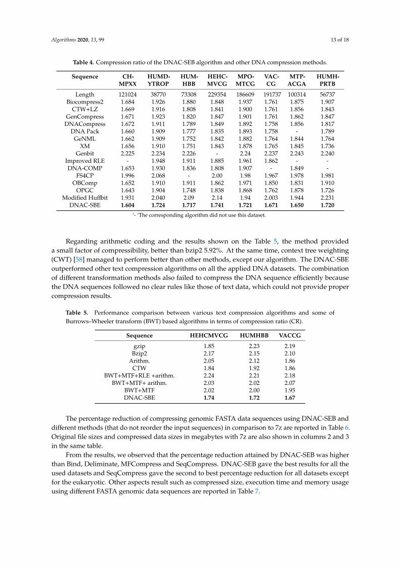
To assess the efficiency of the proposed method, its compression performance was compared withthe other lossless DNA compressors, namely Biocompress-2 [5], DNACompress [32], DNAPack [16],improved RLE [41], DNA-COMPACT (DNA-COMP) [42], Modified HuffBit [48] and others in termsof CR using a real DNA dataset. Moreover, FS4CP [57] and OPGC [49], as well as the OBCompalgorithm [50] were also included in the comparison. Traditional compression algorithms such asgzip [27], bzip2 [28] and arithmetic [47] coding and some of the transformation techniques such asBWT and MTF were also used to compress the DNA sequences. The obtained compression ratios ofthe DNAC-SEB against state-of-the-art algorithms are shown in Tables 3 and 4. It should be noted thatin Tables 4–9, the best results in terms of different compression metrics are shown with a bold font.

Based on Table 4, the proposed technique had a compression ratio as good as the DNA compressionmethod. Note that data pertaining to HUMGHCS, CHMPXX and MTPACGA show excellent results,in which the size was reduced by more than 78%, in particular using DNAC-SBE.

Algorithms 2020, 13, 99 13 of 18

Table 4. Compression ratio of the DNAC-SEB algorithm and other DNA compression methods.

Sequence CH-MPXX

HUMD-YTROP

HUM-HBB

HEHC-MVCG

MPO-MTCG

VAC-CG

MTP-ACGA

HUMH-PRTB

Length 121024 38770 73308 229354 186609 191737 100314 56737Biocompress2 1.684 1.926 1.880 1.848 1.937 1.761 1.875 1.907

CTW+LZ 1.669 1.916 1.808 1.841 1.900 1.761 1.856 1.843GenCompress 1.671 1.923 1.820 1.847 1.901 1.761 1.862 1.847

DNACompress 1.672 1.911 1.789 1.849 1.892 1.758 1.856 1.817DNA Pack 1.660 1.909 1.777 1.835 1.893 1.758 - 1.789

GeNML 1.662 1.909 1.752 1.842 1.882 1.764 1.844 1.764XM 1.656 1.910 1.751 1.843 1.878 1.765 1.845 1.736

Genbit 2.225 2.234 2.226 - 2.24 2.237 2.243 2.240Improved RLE - 1.948 1.911 1.885 1.961 1.862 - -DNA-COMP 1.653 1.930 1.836 1.808 1.907 - 1.849 -

FS4CP 1.996 2.068 - 2.00 1.98 1.967 1.978 1.981OBComp 1.652 1.910 1.911 1.862 1.971 1.850 1.831 1.910

OPGC 1.643 1.904 1.748 1.838 1.868 1.762 1.878 1.726Modified Huffbit 1.931 2.040 2.09 2.14 1.94 2.003 1.944 2.231

DNAC-SBE 1.604 1.724 1.717 1.741 1.721 1.671 1.650 1.720

‘- ‘The corresponding algorithm did not use this dataset.

Regarding arithmetic coding and the results shown on the Table 5, the method provideda small factor of compressibility, better than bzip2 5.92%. At the same time, context tree weighting(CWT) [58] managed to perform better than other methods, except our algorithm. The DNAC-SBEoutperformed other text compression algorithms on all the applied DNA datasets. The combinationof different transformation methods also failed to compress the DNA sequence efficiently becausethe DNA sequences followed no clear rules like those of text data, which could not provide propercompression results.

Table 5. Performance comparison between various text compression algorithms and some ofBurrows–Wheeler transform (BWT) based algorithms in terms of compression ratio (CR).

Sequence HEHCMVCG HUMHBB VACCG

gzip 1.85 2.23 2.19Bzip2 2.17 2.15 2.10

Arithm. 2.05 2.12 1.86CTW 1.84 1.92 1.86

BWT+MTF+RLE +arithm. 2.24 2.21 2.18BWT+MTF+ arithm. 2.03 2.02 2.07

BWT+MTF 2.02 2.00 1.95DNAC-SBE 1.74 1.72 1.67

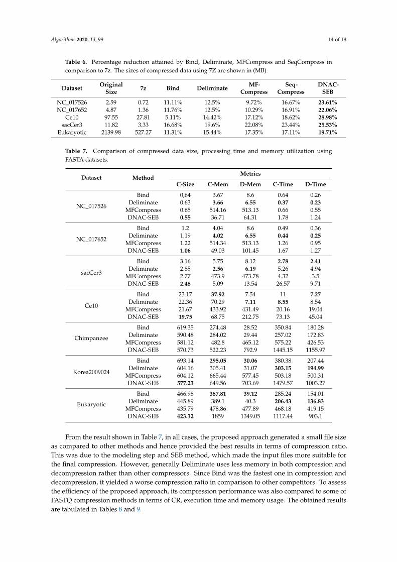
The percentage reduction of compressing genomic FASTA data sequences using DNAC-SEB anddifferent methods (that do not reorder the input sequences) in comparison to 7z are reported in Table 6.Original file sizes and compressed data sizes in megabytes with 7z are also shown in columns 2 and 3in the same table.

From the results, we observed that the percentage reduction attained by DNAC-SEB was higherthan Bind, Deliminate, MFCompress and SeqCompress. DNAC-SEB gave the best results for all theused datasets and SeqCompress gave the second to best percentage reduction for all datasets exceptfor the eukaryotic. Other aspects result such as compressed size, execution time and memory usageusing different FASTA genomic data sequences are reported in Table 7.

Algorithms 2020, 13, 99 14 of 18

Table 6. Percentage reduction attained by Bind, Deliminate, MFCompress and SeqCompress incomparison to 7z. The sizes of compressed data using 7Z are shown in (MB).

Dataset OriginalSize 7z Bind Deliminate MF-

CompressSeq-

CompressDNAC-

SEB

NC_017526 2.59 0.72 11.11% 12.5% 9.72% 16.67% 23.61%NC_017652 4.87 1.36 11.76% 12.5% 10.29% 16.91% 22.06%

Ce10 97.55 27.81 5.11% 14.42% 17.12% 18.62% 28.98%sacCer3 11.82 3.33 16.68% 19.6% 22.08% 23.44% 25.53%

Eukaryotic 2139.98 527.27 11.31% 15.44% 17.35% 17.11% 19.71%

Table 7. Comparison of compressed data size, processing time and memory utilization usingFASTA datasets.

Dataset MethodMetrics

C-Size C-Mem D-Mem C-Time D-Time

NC_017526

Bind 0,64 3.67 8.6 0.64 0.26Deliminate 0.63 3.66 6.55 0.37 0.23

MFCompress 0.65 514.16 513.13 0.66 0.55DNAC-SEB 0.55 36.71 64.31 1.78 1.24

NC_017652

Bind 1.2 4.04 8.6 0.49 0.36Deliminate 1.19 4.02 6.55 0.44 0.25

MFCompress 1.22 514.34 513.13 1.26 0.95DNAC-SEB 1.06 49.03 101.45 1.67 1.27

sacCer3

Bind 3.16 5.75 8.12 2.78 2.41Deliminate 2.85 2.56 6.19 5.26 4.94

MFCompress 2.77 473.9 473.78 4.32 3.5DNAC-SEB 2.48 5.09 13.54 26.57 9.71

Ce10

Bind 23.17 37.92 7.54 11 7.27Deliminate 22.36 70.29 7.11 8.55 8.54

MFCompress 21.67 433.92 431.49 20.16 19.04DNAC-SEB 19.75 68.75 212.75 73.13 45.04

Chimpanzee

Bind 619.35 274.48 28.52 350.84 180.28Deliminate 590.48 284.02 29.44 257.02 172.83

MFCompress 581.12 482.8 465.12 575.22 426.53DNAC-SEB 570.73 522.23 792.9 1445.15 1155.97

Korea2009024

Bind 693.14 295.05 30.06 380.38 207.44Deliminate 604.16 305.41 31.07 303.15 194.99

MFCompress 604.12 665.44 577.45 503.18 500.31DNAC-SEB 577.23 649.56 703.69 1479.57 1003.27

Eukaryotic

Bind 466.98 387.81 39.12 285.24 154.01Deliminate 445.89 389.1 40.3 206.43 136.83

MFCompress 435.79 478.86 477.89 468.18 419.15DNAC-SEB 423.32 1859 1349.05 1117.44 903.1

From the result shown in Table 7, in all cases, the proposed approach generated a small file sizeas compared to other methods and hence provided the best results in terms of compression ratio.This was due to the modeling step and SEB method, which made the input files more suitable forthe final compression. However, generally Deliminate uses less memory in both compression anddecompression rather than other compressors. Since Bind was the fastest one in compression anddecompression, it yielded a worse compression ratio in comparison to other competitors. To assessthe efficiency of the proposed approach, its compression performance was also compared to some ofFASTQ compression methods in terms of CR, execution time and memory usage. The obtained resultsare tabulated in Tables 8 and 9.

Algorithms 2020, 13, 99 15 of 18

From Table 8 values, it is clear that the proposed method achieved a better compression ratiothan other methods on all the applied dataset. In all cases, DNAC-SEB generated low file size ascompared to other algorithms and hence a better compression ratio. Using ERR005143_1 dataset,DNAC-SEB shows an improvement of 4.78% and 3.52% to GTZ and Fqzcomp, respectively. The FASTQfile compressors, including Fqzcomp [11], Quip [53], DSRC [10] and gzip [27], were compared and theresults are reported in Table 9.

Table 8. Compression ratios of different tools on 4 FASTQ datasets.

Dataset Original Size (MB) gzip DSRC Quip Fqzcomp GTZ DNAC-SEB

ERR005143_1 121.92 1.020 0.238 0.250 0.227 0.230 0.219ERR005143_2 121.92 1.086 0.249 0.239 0.229 0.230 0.219SRR554369_1 158.11 0.209 0.250 0.223 0.222 0.233 0.220SRR554369_2 158.11 0.209 0.249 0.227 0.222 0.234 0.220

Table 9. Comparison of compressed data size, processing time and memory utilization usingFASTQ datasets.

Dataset MethodMetrics

C-Size C-Mem D-Mem C-Time D-Time

ERR005143_1

DSRC 30.46 166.45 100.56 5.54 3.4Quip 28.96 393.7 389.02 10.63 22.09

Fqzcomp 27.73 79.46 67.33 7.88 10.08Gzip 124.36 0.86 1.39 28.94 2.7

DNAC-SEB 26.81 580.38 563,91 38.08 18.64

ERR005143_2

DSRC 30.41 168.56 106.5 5.83 4.09Quip 29.25 395.25 389.54 11.07 23.95

Fqzcomp 27.9 79.46 59.3 8.45 10.35Gzip 132.42 0.86 1.39 29.45 2.79

DNAC-SEB 26.28 580.57 524.57 72.06 20.54

SRR554369_1

DSRC 39.52 183.42 152.65 4.11 4.46Quip 35.26 383.95 382.59 10.86 22.93

Fqzcomp 35.13 79.47 67.34 7.21 10.4Gzip 45.97 0.87 1.39 28.51 1.05

DNAC-SEB 34.9 702.18 615.97 43.71 31.34

SRR554369_2

DSRC 39.38 173.57 132.1 4.23 4.6Quip 35.93 383.84 382.1 11.63 23.62

Fqzcomp 35.12 66.41 57.179 7.86 10.52Gzip 45.89 0.87 1.39 27.98 1.05

DNAC-SEB 34.84 781.98 644.66 43.18 30.8

The results of FASTQ file compression with different compressors show that DNAC-SEBoutperformed existing tools in terms of compression ratios for all types of FASTQ benchmarkdatasets. From the experimental results, we could observe that the best compression ratio, minimummemory and maximum speed requirements were competing goals. Generally, the higher compressionrates were achieved by compressors that were slower and required higher memory. For example,Gzip had the best performance in the case of memory and decompression speed usage but offered thelowest compression ratio, which provided valuable long-term space and bandwidth savings. When thedata size was an important aspect, tools such as DNAC-SEB were crucial.

4. Conclusions

In this paper, the authors described a new reference-free DNA compressor (DNAC-SBE), a losslesshybrid compressor that consisted of three phases, to compress any type of DNA sequences. The obtained

Algorithms 2020, 13, 99 16 of 18

results show that DNAC-SBE outperformed some of the state-of-the-art compressors on the benchmarkperformed in terms of the compression ratio, regardless of the file format or data size. The proposedalgorithm compressed both repeated and non-repeated sequences, not depending on any specificpatterns or parameters and accepting data from all kinds of platforms. An important achievement ofthe paper was that it took into consideration the appearance of an unidentified base found in DNA datasequences, ignored by most of the other compression methods. Another advantage of this approachwas that the DNAC-SEB compressor guaranteed the full recovery of the original data. The design ofDNAC-SBE was simple and flexible, showing good compression rates compared to an important partof other similar algorithms.

DNAC-SEB is more suitable when the compressed data, storage space and data transfer werecrucial. More efforts will be made in the future to optimize memory utilization and compression speed.

Author Contributions: Conceptualization, D.M., X.Y. and A.S.; methodology, D.M.; software, D.M. and A.S.;validation, D.M., X.Y. and A.S.; Data curation, D.M.; The paper was initially drafted by D.M. and revised By D.M.,X.Y. and A.S.; supervision, X.Y.; All authors have read and agreed to the published version of the manuscript.This work was supported by WHUT (Wuhan University of Technology) university. The authors are grateful forthis support.

Funding: This research received no external funding.

Acknowledgments: This work was supported by WHUT (Wuhan University of Technology) university.The authors are grateful for this support. We would also like to thank the authors of evaluated compression toolsfor providing support for their tools.

Conflicts of Interest: The authors declare no conflict of interest.

Availability of Data and Materials: Some of the datasets cited used in this study were downloaded from NCBIsequence read archive (SRA) from the URL ftp://ftp.ncbi.nih.gov/genomes/. And some of them are obtained fromUCSC database from the URL: ftp://hgdownload.soe.ucsc.edu/goldenPath. The FASTQ datasets were downloadfrom the URL: ftp://ftp.sra.ebi.ac.uk/vol1/fastq/.

References

1. Lander, E.S.; Linton, L.M.; Birren, B.; Nusbaum, C.; Zody, M.C.; Baldwin, J.; Devon, K.; Dewar, K.; Doyle, M.;FitzHugh, W.; et al. Initial sequencing and analysis of the human genome. Nature 2001, 409, 860–921.[PubMed]

2. Saada, B.; Zhang, J. Vertical DNA sequences compression algorithm based on hexadecimal representation.In Proceedings of the World Congress on Engineering and Computer Science, San Francisco, CA, USA, 21–23October 2015; pp. 21–25.

3. Jahaan, A.; Ravi, T.; Arokiaraj, S. A comparative study and survey on existing DNA compression techniques.Int. J. Adv. Res. Comput. Sci. 2017, 8, 732–735.

4. Rajarajeswari, P.; Apparao, A. DNABIT Compress–Genome compression algorithm. Bioinformation 2011, 5,350. [CrossRef] [PubMed]

5. Grumbach, S.; Tahi, F. A new challenge for compression algorithms: Genetic sequences. Information Process.Manag. 1994, 30, 875–886. [CrossRef]

6. Majumder, A.B.; Gupta, S. CBSTD: A Cloud Based Symbol Table Driven DNA Compressions Algorithm.In Industry Interactive Innovations in Science, Engineering and Technology; Springer: Singapore, 2018; pp. 467–476.

7. Mohammed, M.H.; Dutta, A.; Bose, T.; Chadaram, S.; Mande, S.S. DELIMINATE—a fast and efficient methodfor loss-less compression of genomic sequences: Sequence analysis. Bioinformatics 2012, 28, 2527–2529.[CrossRef]

8. Pinho, A.J.; Pratas, D. MFCompress: A compression tool for FASTA and multi-FASTA data. Bioinformatics2014, 30, 117–118. [CrossRef]

9. Sardaraz, M.; Tahir, M.; Ikram, A.A.; Bajwa, H. SeqCompress: An algorithm for biological sequencecompression. Genomics 2014, 104, 225–228. [CrossRef]

10. Deorowicz, S.; Grabowski, S. Compression of DNA sequence reads in FASTQ format. Bioinformatics 2011, 27,860–862. [CrossRef]

11. Bonfield, J.K.; Mahoney, M.V. Compression of FASTQ and SAM format sequencing data. PloS ONE 2013, 8,e59190. [CrossRef]

Algorithms 2020, 13, 99 17 of 18

12. Aly, W.; Yousuf, B.; Zohdy, B. A Deoxyribonucleic acid compression algorithm using auto-regression andswarm intelligence. J. Comput. Sci. 2013, 9, 690–698. [CrossRef]

13. Hosseini, M.; Pratas, D.; Pinho, A.J. A survey on data compression methods for biological sequences.Information 2016, 7, 56. [CrossRef]

14. Numanagic, I.; Bonfield, J.K.; Hach, F.; Voges, J.; Ostermann, J.; Alberti, C.; Mattavelli, M.; Sahinalp, S.C.Comparison of high-throughput sequencing data compression tools. Nat. Methods 2016, 13, 1005. [CrossRef]

15. Xing, Y.; Li, G.; Wang, Z.; Feng, B.; Song, Z.; Wu, C. GTZ: A fast compression and cloud transmission tooloptimized for FASTQ files. BMC bioinformatics 2017, 18, 549. [CrossRef] [PubMed]

16. Behzadi, B.; Le Fessant, F. DNA compression challenge revisited: A dynamic programming approach.In Proceedings of the Annual Symposium on Combinatorial Pattern Matching, Heidelberg, Jeju Island,Korea, 19–22 June 2005; pp. 190–200.

17. Kuruppu, S.; Puglisi, S.J.; Zobel, J. Reference sequence construction for relative compression of genomes.In Proceedings of the International Symposium on String Processing and Information Retrieval, Pisa, Italy;2011; pp. 420–425.

18. GenBank and WGS Statistics (NCBI). Available online: https://www.ncbi.nlm.nih.gov/genbank/statistics/(accessed on 29 June 2019).

19. 1000 Genomes Project Consortium “a map of human genome variation from population-scale sequencing”,Nature 467 (2010) 1061–1073. Available online: www.1000genomes.org/ (accessed on 19 April 2020).

20. Consortium, E.P. The ENCODE (ENCyclopedia of DNA elements) project. Science 2004, 306, 636–640.[CrossRef] [PubMed]

21. Keerthy, A.; Appadurai, A. An empirical study of DNA compression using dictionary methods and patternmatching in compressed sequences. IJAER 2015, 10, 35064–35067.

22. Arya, G.P.; Bharti, R.; Prasad, D.; Rana, S.S. An Improvement over direct coding technique to compressrepeated & non-repeated nucleotide data. In Proceedings of the 2016 International Conference on Computing,Communication and Automation (ICCCA), Noida, India, 29–30 April 2016; pp. 193–196.

23. Rastogi, K.; Segar, K. Analysis and performance comparison of lossless compression techniques for text data.Int. J. Eng. Comput. Res. 2014, 3, 123–127.

24. Singh, A.V.; Singh, G. A survey on different text data compression techniques. Int. J. Sci. Res. 2012, 3,1999–2002.

25. Al-Okaily, A.; Almarri, B.; Al Yami, S.; Huang, C.-H. Toward a Better Compression for DNA SequencesUsing Huffman Encoding. J. Comput. Biol. 2017, 24, 280–288. [CrossRef]

26. Sharma, K.; Gupta, K. Lossless data compression techniques and their performance. In Proceedings of the2017 International Conference on Computing, Communication and Automation (ICCCA), Greater Noida,India, 5–6 May 2017; pp. 256–261.

27. Gzip. Available online: http://www.gzip.org/ (accessed on 29 June 2019).28. Bzip. Available online: http://www.bzip.org/ (accessed on 29 June 2019).29. Bakr, N.S.; Sharawi, A.A. DNA lossless compression algorithms. Am. J. Bioinformatics Res. 2013, 3, 72–81.30. Grumbach, S.; Tahi, F. Compression of DNA sequences. In Proceedings of the Data Compression

Confonference (DCC-93), Snowbird, UT, USA, 30 March–2 April 1993; pp. 340–350.31. Chen, X.; Kwong, S.; Li, M. A compression algorithm for DNA sequences and its applications in genome

comparison. Genome Inf. 1999, 10, 51–61.32. Chen, X.; Li, M.; Ma, B.; Tromp, J. DNACompress: Fast and effective DNA sequence compression.

Bioinformatics 2002, 18, 1696–1698. [CrossRef] [PubMed]33. Korodi, G.; Tabus, I. An Efficient Normalized Maximum Likelihood Algorithm for DNA Sequence

Compression. ACM Trans. Inf. Syst. 2005, 23, 3–34. [CrossRef]34. Tan, L.; Sun, J.; Xiong, W. A Compression Algorithm for DNA Sequence Using Extended Operations.

J. Comput. Inf. Syst. 2012, 8, 7685–7691.35. Ma, B.; Tromp, J.; Li, M. PatternHunter—Faster and more sensitive homology search. Bioinformatics 2002, 18,

440–445. [CrossRef]36. Tabus, I.; Korodi, G.; Rissanen, J. DNA sequence compression using the normalized maximum likelihood

model for discrete regression. In Proceedings of the Data Compression Conference (DCC ’03), Snowbird, UT,USA, 25–27 March 2003; pp. 253–262.

Algorithms 2020, 13, 99 18 of 18

37. Cao, M.D.; Dix, T.I.; Allison, L.; Mears, C. A simple statistical algorithm for biological sequence compression.In Proceedings of the 2007 Data Compression Conference (DCC’07), Snowbird, UT, USA, 27–29 March 2007;pp. 43–52.

38. Mishra, K.N.; Aaggarwal, A.; Abdelhadi, E.; Srivastava, D. An efficient horizontal and vertical method foronline DNA sequence compression. Int. J. Comput. Appl. 2010, 3, 39–46. [CrossRef]

39. Rajeswari, P.R.; Apparo, A.; Kumar, V. GENBIT COMPRESS TOOL (GBC): A java-based tool to compressDNA sequences and compute compression ratio (bits/base) of genomes. Int. J. Comput. Sci. Inform. Tech.2010, 2, 181–191.

40. Rajeswari, P.R.; Apparao, A.; Kumar, R.K. Huffbit compress—Algorithm to compress DNA sequences usingextended binary trees. J. Theor. Appl. Inform. Tech. 2010, 13, 101–106.

41. Ouyang, J.; Feng, P.; Kang, J. Fast compression of huge DNA sequence data. In Proceedings of the 2012 5thInternational Conference on BioMedical Engineering and Informatics, Chongqing, China, 16–18 October2012; pp. 885–888.

42. Li, P.; Wang, S.; Kim, J.; Xiong, H.; Ohno-Machado, L.; Jiang, X. DNA-COMPACT: DNA compression based ona pattern-aware contextual modeling technique. PLoS ONE 2013, 8, e80377. [CrossRef]

43. Roy, S.; Bhagot, A.; Sharma, K.A.; Khatua, S. SBVRLDNAComp: An Effective DNA Sequence CompressionAlgorithm. Int. J. Comput. Sci. Appl. 2015, 5, 73–85.

44. Roy, S.; Mondal, S.; Khatua, S.; Biswas, M. An Efficient Compression Algorithm for Forthcoming NewSpecies. Int. J. Hybrid Inf. Tech. 2015, 8, 323–332. [CrossRef]

45. Eric, P.V.; Gopalakrishnan, G.; Karunakaran, M. An optimal seed-based compression algorithm for DNAsequences. Adv. Bioinform. 2016. [CrossRef] [PubMed]

46. Rexline, S.J.; Aju, R.G.; Trujilla, L.F. Higher compression from burrows-wheeler transform for DNA sequence.Int. J. Comput. Appl. 2017, 173, 11–15.

47. Keerthy, A.; Priya, S.M. Lempel-Ziv-Welch Compression of DNA Sequence Data with Indexed MultipleDictionaries. Int. J. Appl. Eng. Res. 2017, 12, 5610–5615.

48. Habib, N.; Ahmed, K.; Jabin, I.; Rahman, M.M. Modified HuffBit Compress Algorithm–An Application of R.J. Integr. Bioinform. 2018. [CrossRef] [PubMed]

49. Chen, M.; Li, R.; Yang, L. Optimized Context Weighting for the Compression of the Un-repetitive GenomeSequence Fragment. Wirel. Personal Commun. 2018, 103, 921–939. [CrossRef]

50. Mansouri, D.; Yuan, X. One-Bit DNA Compression Algorithm. In Proceedings of the International Conferenceon Neural Information Processing, Siam reap, Cambodia, 13–16 December 2018; Springer: Siam reap,Cambodia; pp. 378–386.

51. Priyanka, M.; Goel, S. A compression algorithm for DNA that uses ASCII values. In Proceedings of the 2014IEEE International Advance Computing Conference, Gurgaon, India, 21–22 February 2014; pp. 739–743.

52. Bose, T.; Mohammed, M.H.; Dutta, A.; Mande, S.S. BIND–An algorithm for loss-less compression ofnucleotide sequence data. J. Biosci. 2012, 37, 785–789. [CrossRef]

53. Jones, D.; Ruzzo, W.; Peng, X.; Katze, M. Compression of next-generation sequencing reads aided by highlyefficient de novo assembly. Nucleic Acids Res. 2012, 40. [CrossRef]

54. Uthayakumar, J.; Vengattaraman, T.; Dhavachelvan, P. A new lossless neighborhood indexing sequence (NIS)algorithm for data compression in wireless sensor networks. Ad Hoc Netw. 2019, 83, 149–157.

55. Bakr, N.S.; Sharawi, A.A. Improve the compression of bacterial DNA sequence. In Proceedings of the2017 13th International Computer Engineering Conference (ICENCO), Cairo, Egypt, 27–28 December 2017;pp. 286–290.

56. National Center for Biotechnology Information. Available online: https://www.ncbi.nlm.nih.gov/ (accessedon 30 March 2019).

57. Roy, S.; Khatua, S. DNA data compression algorithms based on redundancy. Int. J. Found. Comput. Sci. Technol.2014, 4, 49–58. [CrossRef]

58. Willems, F.M.J.; Shtarkov, Y.M.; Tjalkens, T.J. The context tree weighting method: Basic properties. IEEE Trans.Inf. Theory 1995, 41, 653–664. [CrossRef]

© 2020 by the authors. Licensee MDPI, Basel, Switzerland. This article is an open accessarticle distributed under the terms and conditions of the Creative Commons Attribution(CC BY) license (http://creativecommons.org/licenses/by/4.0/).