1

A New Measure of Earnings surprises and

Post-Earnings-Announcement Drift

By Zhipeng Yan amp Yan Zhaodiams

First draft Sept 2006

This draft Aug 2008

Abstract

In this article we develop a new measure of earnings surprises ndash the earnings surprise elasticity

(ESE) which is defined as the absolute value of earnings announcement abnormal returns (EARs)

scaled by earnings surprises (in percentage) The numerator of the ESE captures all the information

released around earnings announcement dates and market reactions to the information the

denominator of the ESE gives special emphasis to earnings surprises We explore the ESE under four

different categories in terms of the signs of earnings surprises (+-) and the signs of EARs (+-) We

find that a) Across all four sub-samples larger firms have smaller earnings surprises and higher

EARs (both in absolute values) thus have higher ESE quintiles b) Firms in the highest ESE quintile

usually have much smaller post-earnings-announcement cumulative abnormal returns (CARs) in

absolute value than firms in the lowest ESE quintile c) Against conventional wisdom for around

36 of total observations earnings surprises and EARs move in opposite directions d) More than

11 firms have no surprises those are larger firms with larger institutional shareholdings and

followed by more analysts It is not wise to invest in this group of firms as evidenced in the negative

post-earnings-announcement CARs e) A trading strategy of taking a long position in firms in the

lowest ESE quintile when both earnings surprises and EARs are positive and a short position in

firms in the lowest ESE quintile when both are negative can generate 519 quarterly abnormal

return

School of Management New Jersey Institute of Technology zhipengyannjitedu

diamsInternational Business School Brandeis University heidifoxbrandeisedu

We thank Blake LeBaron Carol Osler Laarni Bulan Wayne Ferson Ming Huang and George Hall seminar

participants at Brandeis University for helpful comments and suggestions As is customary however we accept full

responsibility for any remaining errors

2

1 Introduction

Post-earnings-announcement drift (PEAD) is the tendency for stocks to earn abnormally

high (low) returns in the weeks or even months following a surprisingly positive (negative)

earnings announcement That is if a firmrsquos announced earnings exceed (fall short of) the

market expectation the subsequent abnormal returns to its stocks are usually above (below)

normal for weeks or even months It is one of the best documented anomalies above

suspicion (Fama (1998)) and poses ldquothe most severe challenge to financial theoristsrdquo

(Brennan (1991)) In this paper we aim to add a new dimension to this anomaly by exploring

a new measure of earnings surprises

Most prior PEAD studies use Standardized Unexpected Earnings (SUE) to measure the

earnings surprises SUE is defined as the difference between actual and expected earnings

scaled by the standard deviation of the forecast errors during the estimation period where

expected earnings are estimated either from analystsrsquo forecasts or from a time series model

of earnings A major downside of SUE is that although it captures the earnings surprises it

neither captures other new information that might also be unveiled around earnings

announcement dates nor does it capture the market reactions to the information

To capture both earnings surprises and stock market reactions to all the information

disclosed around earnings announcement dates we develop a new measure - the earnings

surprise elasticity (ESE) We define it as the absolute value of earnings announcement

abnormal returns (EARs) scaled by earnings surprises (in percentage) Since stock return is

in fact the percentage change in stock price if there is no dividend paid out this ratio is

actually an elasticity measure - the percentage change in stock prices that occurs in response

to a percent change in earnings surprises We further explore the ESE under four different

categories in terms of the signs of earnings surprises (+-) and the signs of EARs (+-)

Within each category we sort firms into quintiles based on the ESE ranks The ESE

measure together with the four-category classification has two advantages over the

commonly used SUE measure

First actual earnings are the most important information disclosed by a firm on earnings

announcement dates (by definition) The denominator of the ESE measures new information

contained in actual earnings the difference between actual and expected earnings Of course

3

firms also release other information which may not be as important as earnings but can still

give investors a better understanding of the future of the firms and its competitive

environment such as sales inventories and other forward-looking information All the

information earnings related or non-earnings related is impounded into the numerator of the

ESE ndash the EARs ndash while the SUE measure is totally silent on stock market reactions around

earnings announcement dates

Second we live in a world where lsquoprofit is kingrsquo It is conventional wisdom that positive

(negative) earnings surprises shall lead to positive (negative) stock responses around

earnings announcement dates Surprisingly we find that around 36 of total observations

are against this ldquoconventional wisdomrdquo That is in more than one third cases positive

(negative) earnings surprises lead to negative (positive) stock responses around earnings

announcement dates By grouping the stocks into four different categories in terms of signs

of earnings surprises (+-) and EARs (+-) we can differentiate those ldquoanomaliesrdquo from the

ldquoconventional wisdomrdquo and tell how significant the other news is SUE is helpless in this

regard

We have a number of new findings in this paper

1) Across all four sub-samples larger firms have smaller earnings surprises and higher

EARs (in absolute values) thus have higher ESE quintiles and are followed by smaller drifts

subsequently This finding is different from prior works (Chan Jegadeesh and Lakonishok

(1996) and Brandt et al (2006)) they find larger EARs lead to larger drifts in the subsequent

periods

2) When earnings surprises and EARs move in the same direction (53 of the total

observations) post-earnings-announcement cumulative abnormal returns (CARs) have the

same signs as those of earnings surprises in each ESE quintile Firms in the higher ESE

quintiles usually have much smaller post-earnings-announcement CARs (in absolute value)

than firms in the lower ESE quintiles

3) When earnings surprises and EARs move in opposite directions (36 of the total

observations) there must be some extraordinary good news for a stock to have a positive

response to the negative earnings surprise and extraordinary bad news for a stock to have a

negative reaction to the positive earnings surprise When this is the case post-earnings-

4

announcement CARs usually still have the same signs as those of earnings surprises

4) When Earnings surprise equal to zero (11 of the total observations) the ESE is not

defined Firms in this group are larger firms with larger institutional shareholdings and

followed by more analysts It is not wise to invest in this group of firms as evidenced in the

negative post-earnings-announcement CARs Also it may suggest that faced with intense

pressure to meet earnings estimates from analysts and investors the executives in these firms

may smooth earnings over accounting periods to achieve the forecasted result However the

subsequent negative CARs reflect that the firmsrsquo operations might not be as good as the

earnings information shows

5) A strategy of a long position in firms in the lowest ESE quintile when both earnings

surprises and EARs are positive and a short position in firms in the lowest ESE quintile

when both are negative can generate 519 quarterly abnormal return (before transaction

costs)

6) The ESE has a significant impact on post-earnings-announcement CARs after

controlling for market-related variables ndash book-to-market ratio transaction costs investorsrsquo

sophistication and arbitrage risk ndash and financial statement variables ndash inventory accounts

receivable gross margin and selling and administrative expenses

This paper offers four contributions to the existing literature First we add to the

literature on drifts by documenting the market reactions to both earnings news and

information beyond earnings news Second by grouping firms into 4 categories we discover

a different phenomenon from prior work larger EARs lead to smaller drifts in the

subsequent periods prior works (Chan Jegadeesh and Lakonishok (1996) and Brandt et al

(2006)) find larger EARs lead to larger drifts in the subsequent periods Third we unearth a

new anomaly that the ESE can also lead to predictable returns in the future Fourth prior

studies only examine the effect of market-related variables on drifts we not only control the

market-related variables but also study the effect of additional financial statement variables

on drifts

The rest of the paper is organized as follows Section 2 reviews the prior literature

Section 3 explains the sample selection and methodology Section 4 presents the empirical

findings Section 5 performs robustness checks and Section 6 concludes the paper

5

2 Prior research and motivation

The post-earnings-announcement drift was first identified by Ball and Brown in the late

1960s This predictability of stock returns after earnings announcements had attracted

substantial research and has been documented consistently in numerous papers over the

decades Rendleman Jones and Latane (1982) Foster Olsen and Shevlin (1984) Bernard

and Thomas (1989) are among the many who replicate the phenomenon with large scale

sample sets They show that a long position in stocks with unexpected earnings in the highest

decile combined with a short position in stocks in the lowest decile yields an estimated high

abnormal return Even recent research such as Collins and Hribar (2000) Liang (2003)

Livnat (2003) Jegadeesh and Livnat (2006) Narayanamoorthy (2003) Francis et al (2004)

Mendenhall (2004) Livnat and Mendenhall (2006) Brandt et al (2006) continue to

document the abnormal return after the earnings announcement

Studies also demonstrate that the magnitude of the drift is different for different subsets

of firms For example Bartov Radhakrishnan and Krinsky (2000) find the drift is smaller

for firms with greater proportions of institutional investors Bhushan (1994) Mikhail

Walther and Willis (2003) show firms followed by more experienced analysts have a smaller

drift Mendenhall (2004) shows the drift is larger for firms subject to higher arbitrage risks

Bhushan (1994) and Stoll (2000) show recent stock prices and recent dollar trading volumes

are significantly associated with the transaction costs the drift is larger for firms subject to

higher trading costs Bernard and Thomas (1989) and Bartov Radhakrishnan and Krinsky

(2000) find the drift is smaller for larger firms and larger for smaller firms The above

research efforts identify the factors that are associated with different drift levels

All these drift studies predominantly focus on earnings surprises and very little attention

is paid to other unveiled information around earnings announcement dates or market reaction

to this information The commonly used earnings surprises measure SUE is totally silent

when other important news is released with the earnings announcement12

1 For example Apple Computer Inc released quarterly earnings on Jan 17 2001 Although the earnings were below

expectations analysts were cheered by news that the company had sharply cut inventories of computers on retailers

shelves Apples shares jumped 11 the following day The Wall Street Journal ldquoMore Questions About Options for

Applerdquo August 7 2006 2 For another example on May 4 2006 Procter amp Gamble Co reported net sales rose 21 to $1725 billion and

earnings rose to 63 cents a share for the quarter ended March 31 which was higher than expected earnings of 61 cents

3

firms also release other information which may not be as important as earnings but can still

give investors a better understanding of the future of the firms and its competitive

environment such as sales inventories and other forward-looking information All the

information earnings related or non-earnings related is impounded into the numerator of the

ESE ndash the EARs ndash while the SUE measure is totally silent on stock market reactions around

earnings announcement dates

Second we live in a world where lsquoprofit is kingrsquo It is conventional wisdom that positive

(negative) earnings surprises shall lead to positive (negative) stock responses around

earnings announcement dates Surprisingly we find that around 36 of total observations

are against this ldquoconventional wisdomrdquo That is in more than one third cases positive

(negative) earnings surprises lead to negative (positive) stock responses around earnings

announcement dates By grouping the stocks into four different categories in terms of signs

of earnings surprises (+-) and EARs (+-) we can differentiate those ldquoanomaliesrdquo from the

ldquoconventional wisdomrdquo and tell how significant the other news is SUE is helpless in this

regard

We have a number of new findings in this paper

1) Across all four sub-samples larger firms have smaller earnings surprises and higher

EARs (in absolute values) thus have higher ESE quintiles and are followed by smaller drifts

subsequently This finding is different from prior works (Chan Jegadeesh and Lakonishok

(1996) and Brandt et al (2006)) they find larger EARs lead to larger drifts in the subsequent

periods

2) When earnings surprises and EARs move in the same direction (53 of the total

observations) post-earnings-announcement cumulative abnormal returns (CARs) have the

same signs as those of earnings surprises in each ESE quintile Firms in the higher ESE

quintiles usually have much smaller post-earnings-announcement CARs (in absolute value)

than firms in the lower ESE quintiles

3) When earnings surprises and EARs move in opposite directions (36 of the total

observations) there must be some extraordinary good news for a stock to have a positive

response to the negative earnings surprise and extraordinary bad news for a stock to have a

negative reaction to the positive earnings surprise When this is the case post-earnings-

4

announcement CARs usually still have the same signs as those of earnings surprises

4) When Earnings surprise equal to zero (11 of the total observations) the ESE is not

defined Firms in this group are larger firms with larger institutional shareholdings and

followed by more analysts It is not wise to invest in this group of firms as evidenced in the

negative post-earnings-announcement CARs Also it may suggest that faced with intense

pressure to meet earnings estimates from analysts and investors the executives in these firms

may smooth earnings over accounting periods to achieve the forecasted result However the

subsequent negative CARs reflect that the firmsrsquo operations might not be as good as the

earnings information shows

5) A strategy of a long position in firms in the lowest ESE quintile when both earnings

surprises and EARs are positive and a short position in firms in the lowest ESE quintile

when both are negative can generate 519 quarterly abnormal return (before transaction

costs)

6) The ESE has a significant impact on post-earnings-announcement CARs after

controlling for market-related variables ndash book-to-market ratio transaction costs investorsrsquo

sophistication and arbitrage risk ndash and financial statement variables ndash inventory accounts

receivable gross margin and selling and administrative expenses

This paper offers four contributions to the existing literature First we add to the

literature on drifts by documenting the market reactions to both earnings news and

information beyond earnings news Second by grouping firms into 4 categories we discover

a different phenomenon from prior work larger EARs lead to smaller drifts in the

subsequent periods prior works (Chan Jegadeesh and Lakonishok (1996) and Brandt et al

(2006)) find larger EARs lead to larger drifts in the subsequent periods Third we unearth a

new anomaly that the ESE can also lead to predictable returns in the future Fourth prior

studies only examine the effect of market-related variables on drifts we not only control the

market-related variables but also study the effect of additional financial statement variables

on drifts

The rest of the paper is organized as follows Section 2 reviews the prior literature

Section 3 explains the sample selection and methodology Section 4 presents the empirical

findings Section 5 performs robustness checks and Section 6 concludes the paper

5

2 Prior research and motivation

The post-earnings-announcement drift was first identified by Ball and Brown in the late

1960s This predictability of stock returns after earnings announcements had attracted

substantial research and has been documented consistently in numerous papers over the

decades Rendleman Jones and Latane (1982) Foster Olsen and Shevlin (1984) Bernard

and Thomas (1989) are among the many who replicate the phenomenon with large scale

sample sets They show that a long position in stocks with unexpected earnings in the highest

decile combined with a short position in stocks in the lowest decile yields an estimated high

abnormal return Even recent research such as Collins and Hribar (2000) Liang (2003)

Livnat (2003) Jegadeesh and Livnat (2006) Narayanamoorthy (2003) Francis et al (2004)

Mendenhall (2004) Livnat and Mendenhall (2006) Brandt et al (2006) continue to

document the abnormal return after the earnings announcement

Studies also demonstrate that the magnitude of the drift is different for different subsets

of firms For example Bartov Radhakrishnan and Krinsky (2000) find the drift is smaller

for firms with greater proportions of institutional investors Bhushan (1994) Mikhail

Walther and Willis (2003) show firms followed by more experienced analysts have a smaller

drift Mendenhall (2004) shows the drift is larger for firms subject to higher arbitrage risks

Bhushan (1994) and Stoll (2000) show recent stock prices and recent dollar trading volumes

are significantly associated with the transaction costs the drift is larger for firms subject to

higher trading costs Bernard and Thomas (1989) and Bartov Radhakrishnan and Krinsky

(2000) find the drift is smaller for larger firms and larger for smaller firms The above

research efforts identify the factors that are associated with different drift levels

All these drift studies predominantly focus on earnings surprises and very little attention

is paid to other unveiled information around earnings announcement dates or market reaction

to this information The commonly used earnings surprises measure SUE is totally silent

when other important news is released with the earnings announcement12

1 For example Apple Computer Inc released quarterly earnings on Jan 17 2001 Although the earnings were below

expectations analysts were cheered by news that the company had sharply cut inventories of computers on retailers

shelves Apples shares jumped 11 the following day The Wall Street Journal ldquoMore Questions About Options for

Applerdquo August 7 2006 2 For another example on May 4 2006 Procter amp Gamble Co reported net sales rose 21 to $1725 billion and

earnings rose to 63 cents a share for the quarter ended March 31 which was higher than expected earnings of 61 cents

4

announcement CARs usually still have the same signs as those of earnings surprises

4) When Earnings surprise equal to zero (11 of the total observations) the ESE is not

defined Firms in this group are larger firms with larger institutional shareholdings and

followed by more analysts It is not wise to invest in this group of firms as evidenced in the

negative post-earnings-announcement CARs Also it may suggest that faced with intense

pressure to meet earnings estimates from analysts and investors the executives in these firms

may smooth earnings over accounting periods to achieve the forecasted result However the

subsequent negative CARs reflect that the firmsrsquo operations might not be as good as the

earnings information shows

5) A strategy of a long position in firms in the lowest ESE quintile when both earnings

surprises and EARs are positive and a short position in firms in the lowest ESE quintile

when both are negative can generate 519 quarterly abnormal return (before transaction

costs)

6) The ESE has a significant impact on post-earnings-announcement CARs after

controlling for market-related variables ndash book-to-market ratio transaction costs investorsrsquo

sophistication and arbitrage risk ndash and financial statement variables ndash inventory accounts

receivable gross margin and selling and administrative expenses

This paper offers four contributions to the existing literature First we add to the

literature on drifts by documenting the market reactions to both earnings news and

information beyond earnings news Second by grouping firms into 4 categories we discover

a different phenomenon from prior work larger EARs lead to smaller drifts in the

subsequent periods prior works (Chan Jegadeesh and Lakonishok (1996) and Brandt et al

(2006)) find larger EARs lead to larger drifts in the subsequent periods Third we unearth a

new anomaly that the ESE can also lead to predictable returns in the future Fourth prior

studies only examine the effect of market-related variables on drifts we not only control the

market-related variables but also study the effect of additional financial statement variables

on drifts

The rest of the paper is organized as follows Section 2 reviews the prior literature

Section 3 explains the sample selection and methodology Section 4 presents the empirical

findings Section 5 performs robustness checks and Section 6 concludes the paper

5

2 Prior research and motivation

The post-earnings-announcement drift was first identified by Ball and Brown in the late

1960s This predictability of stock returns after earnings announcements had attracted

substantial research and has been documented consistently in numerous papers over the

decades Rendleman Jones and Latane (1982) Foster Olsen and Shevlin (1984) Bernard

and Thomas (1989) are among the many who replicate the phenomenon with large scale

sample sets They show that a long position in stocks with unexpected earnings in the highest

decile combined with a short position in stocks in the lowest decile yields an estimated high

abnormal return Even recent research such as Collins and Hribar (2000) Liang (2003)

Livnat (2003) Jegadeesh and Livnat (2006) Narayanamoorthy (2003) Francis et al (2004)

Mendenhall (2004) Livnat and Mendenhall (2006) Brandt et al (2006) continue to

document the abnormal return after the earnings announcement

Studies also demonstrate that the magnitude of the drift is different for different subsets

of firms For example Bartov Radhakrishnan and Krinsky (2000) find the drift is smaller

for firms with greater proportions of institutional investors Bhushan (1994) Mikhail

Walther and Willis (2003) show firms followed by more experienced analysts have a smaller

drift Mendenhall (2004) shows the drift is larger for firms subject to higher arbitrage risks

Bhushan (1994) and Stoll (2000) show recent stock prices and recent dollar trading volumes

are significantly associated with the transaction costs the drift is larger for firms subject to

higher trading costs Bernard and Thomas (1989) and Bartov Radhakrishnan and Krinsky

(2000) find the drift is smaller for larger firms and larger for smaller firms The above

research efforts identify the factors that are associated with different drift levels

All these drift studies predominantly focus on earnings surprises and very little attention

is paid to other unveiled information around earnings announcement dates or market reaction

to this information The commonly used earnings surprises measure SUE is totally silent

when other important news is released with the earnings announcement12

1 For example Apple Computer Inc released quarterly earnings on Jan 17 2001 Although the earnings were below

expectations analysts were cheered by news that the company had sharply cut inventories of computers on retailers

shelves Apples shares jumped 11 the following day The Wall Street Journal ldquoMore Questions About Options for

Applerdquo August 7 2006 2 For another example on May 4 2006 Procter amp Gamble Co reported net sales rose 21 to $1725 billion and

earnings rose to 63 cents a share for the quarter ended March 31 which was higher than expected earnings of 61 cents

5

2 Prior research and motivation

The post-earnings-announcement drift was first identified by Ball and Brown in the late

1960s This predictability of stock returns after earnings announcements had attracted

substantial research and has been documented consistently in numerous papers over the

decades Rendleman Jones and Latane (1982) Foster Olsen and Shevlin (1984) Bernard

and Thomas (1989) are among the many who replicate the phenomenon with large scale

sample sets They show that a long position in stocks with unexpected earnings in the highest

decile combined with a short position in stocks in the lowest decile yields an estimated high

abnormal return Even recent research such as Collins and Hribar (2000) Liang (2003)

Livnat (2003) Jegadeesh and Livnat (2006) Narayanamoorthy (2003) Francis et al (2004)

Mendenhall (2004) Livnat and Mendenhall (2006) Brandt et al (2006) continue to

document the abnormal return after the earnings announcement

Studies also demonstrate that the magnitude of the drift is different for different subsets

of firms For example Bartov Radhakrishnan and Krinsky (2000) find the drift is smaller

for firms with greater proportions of institutional investors Bhushan (1994) Mikhail

Walther and Willis (2003) show firms followed by more experienced analysts have a smaller

drift Mendenhall (2004) shows the drift is larger for firms subject to higher arbitrage risks

Bhushan (1994) and Stoll (2000) show recent stock prices and recent dollar trading volumes

are significantly associated with the transaction costs the drift is larger for firms subject to

higher trading costs Bernard and Thomas (1989) and Bartov Radhakrishnan and Krinsky

(2000) find the drift is smaller for larger firms and larger for smaller firms The above

research efforts identify the factors that are associated with different drift levels

All these drift studies predominantly focus on earnings surprises and very little attention

is paid to other unveiled information around earnings announcement dates or market reaction

to this information The commonly used earnings surprises measure SUE is totally silent

when other important news is released with the earnings announcement12

1 For example Apple Computer Inc released quarterly earnings on Jan 17 2001 Although the earnings were below

expectations analysts were cheered by news that the company had sharply cut inventories of computers on retailers

shelves Apples shares jumped 11 the following day The Wall Street Journal ldquoMore Questions About Options for

Applerdquo August 7 2006 2 For another example on May 4 2006 Procter amp Gamble Co reported net sales rose 21 to $1725 billion and

earnings rose to 63 cents a share for the quarter ended March 31 which was higher than expected earnings of 61 cents

6

Recent efforts to examine whether share prices incorporate other information find some

interesting results For example Jegadeesh and Livnat (2006) show the magnitude of the

drift after earnings announcements is dependent on the sales surprises disclosed

simultaneously with earnings When the two signals confirm each other the magnitude of the

drift is larger a trading strategy based on both earnings and sales surprises yields a higher

abnormal return than a trading strategy which is based only on earnings surprises Rajgopal

Shevlin and Venkatachalam (2003) find investors over-estimate the valuation of order

backlogs that are disclosed in financial statements a long(short) position in the

lowest(highest) decile of order backlog generates significant abnormal returns Gu (2005)

finds patent citation impact is positively associated with future earnings but investors do not

fully incorporate patent impact into stock prices

All of these papers focus on single non-earnings information such as sales surprises

order backlog patent citation and hence limit the generalization of their findings to a

broader set of information Chan Jegadeesh and Lakonishok (1996) and Brandt et al (2006)

shed some light on how to capture a broader set of information and market reactions around

earnings announcement dates by sorting firms on EARs Both papers find that the portfolios

with higher EARs generate substantially higher post-earnings-announcement CARs than the

portfolio with lower EARs Although the EARs measure incorporates all information and

market reactions around earnings announcement dates it doesnrsquot separate the earnings

information from other information Since other investigators have repeatedly found that

earnings forecasts have an important influence on stock prices (see Brown et al (1985))

our paper employs a new measure of surprise ndash ESE ndash which captures all information EARs

captures while giving special emphasis to earnings surprises

3 Sample selection methodology and summary statistics

The mean analyst forecast of quarterly earnings per share (EPS) standard deviation of

the forecasts earnings announcement dates and actual realized EPS are taken from the

a share However analysts surveyed by Thomson Financial had expected higher sales of $176 billion At the end of

the day investors sent PampG shares tumbling disappointed that sales and the companys outlook fell short of analysts

expectations wwwwsjcom ldquothe Evening Wraprdquo May 4 2006

7

Institutional-Brokers-Estimate-System summary statistics files (IBES) To avoid using

stale forecasts we select variable values in the last IBES Statistical Period prior to the

earnings announcement date Our sample period runs from the third quarter of 1985 through

the second quarter of 2005 and we include all the firms from IBES during this period We

match the earnings forecasts for each company with stock daily returns The returns are

provided by the Center for Research on Security Prices (CRSP) at the University of Chicago

Care is taken to adjust for dividends stock splits and stock dividends so that all current and

past returns earnings figures and forecasts are expressed on a comparable basis When we

need book-to-market ratio and other accounting variables we further merge IBES with

Compustat file tape

Prior studies (Foster Olsen and Shevlin (1984) Bernard and Thomas (1898 1990)) show

the magnitude of the earnings related anomalies vary according to firm size to control the

firms-size effect we use value-weighted returns on ten Fama-French portfolios formed on

size as benchmark returns to compute the abnormal returns All the benchmark returns and

breakpoints of each decile are taken from Kenneth Frenchrsquos on-line data library

31 Estimation of SUE ESE and post-earnings-announcement CARs

Following Mendenhall (2004) SUE is defined as actual quarterly EPS minus the latest

mean analyst forecast of quarterly EPS from IBES divided by the standard deviation of the

forecasts

^

^

( )

( )

i q i q

i q

i q

E mean ESUE

std E

minus= ------------------------------------- (1)

Where i qE is the actual EPS for firms i in quarter q ^

( )i qmean E is the mean analyst

forecast of EPS for firms i in quarter q and ^

( )i qstd E is the standard deviation of the

analystsrsquo forecasts for firms i in quarter q

Our alternative measure of the earnings surprises the ESE is the absolute value of the

ratio of EARs over the earnings surprises

8

qi

qiqi rpriseEarningsSu

EARESE

= ------------------------------------ (2)

)(

)(

qi

qiqi

qiEmean

EmeanErpriseEarningsSu

minus=

1 1

1 1

(1 ) (1 )t t

i q i t size t

t t

EAR R R= + =

= minus = minus

= + minus +prod prod

Where qirpriseEarningsSu is measured as the difference between actual and expected

EPS scaled by expected EPS

EARiq is the abnormal return for firms i in quarter q recorded over a three-day window

centered on the announcement date We cumulate returns until one day after the

announcement date to account for two reasons One is for the possibility of firms announcing

earnings after the closing bell The other is for the possibility of delayed stock price reactions

to earnings news particularly since our sample includes NASDAQ issues which may be less

frequently traded (Chan Jegadeesh and Lakonishok (1996)) Rit is the daily return for firms i

in day t Rsizet is the daily value-weighted return on Fama-French size portfolio to which

stock i belongs The ten Fama-French size portfolios are constructed at the end of each June

using the June market equity and NYSE breakpoints

Size adjusted post-earnings-announcement CARs are calculated in a similar manner to

EARs

2 2

(1 ) (1 )t n t n

i n i t size t

t t

CAR R R= =

= =

= + minus +prod prod

Where i nCAR3 is the sized adjusted cumulative abnormal return for firms i from the

second day after the earnings announcement to nth day after the announcement

32 Portfolio assignment

3 Many firms in a few trading days and a few firms in many trading days have missing return values mainly due to

missing prices or not trading on the current exchange We replace the missing values with concurrent benchmark

portfolio returns However to make CAR calculation meaningful we require that the total number of missing days be

less than ten percent of the number of total trading days For instance to calculate 6-month (126 trading days) CARs

if a firm during this 6-month post announcement period have more than 13 missing return values then the 6-month

CAR of this firm for this quarter is excluded from our sample

9

For every quarter between July 1985 and June 2005 we form portfolios as follows

We first group firms into 4 sub-samples in terms of the signs of earnings surprises and

EARs both earnings surprises and EARs are positive both earnings surprises and EARs are

negative earnings surprises are positive while EARs are negative earnings surprises are

negative while EARs are positive

Within each sub-sample we compute the ESE values for every firm We then calculate

quintile breakpoints by ranking the ESE values in the current quarter (rank 1 is the lowest

ESE quintile) By using the current quarterrsquos data instead of the previous quarterrsquos data we

may introduce potential look-ahead bias which assumes that the entire cross-sectional

distribution of the ESE values is known when a firm announces its earnings for quarter q

There are two reasons for us to use the current quarterrsquos data First of all because of

restrictions on sample selection in many cases more than one quarter elapse before the next

earnings announcement data become available for a firm Therefore we cannot get the

lsquopreviousrsquo quarterrsquos data Second most researchers report that post-earnings-announcement

CARs are insensitive to the assignment of firms into a SUE decile using the current quarterrsquos

SUE ranks instead of using SUE cutoffs from the previous quarter (Bernard and

Thomas(1990) Jegadeesh and Livnat (2006)) We also replicate all the results by using the

breakpoints of the distribution of the ESE in the previous quarter The results remain almost

the same

We then examine the pattern of post-earnings-announcement CARs in each ESE quintile

(ESE1 to ESE5) within each sub-sample in subsequent periods starting from the second day

after the earnings announcement up to 5 trading days 10 trading days 1 month (22 trading

days) 2 months (43 trading days) 3 months (63 trading days) 6 months (126 trading days)

9 months (189 trading days) and 1 year (252 trading days) after the earnings announcement

Finally we aim to find the most profitable trading strategy based upon our ESE quintiles

and sub-sample classification The trading strategy is to long the portfolio with the most

positive post-earnings-announcement CARs and short the portfolio with the most negative

post-earnings-announcement CARs These two portfolios may not be in the same sub sample

For comparison we also study no-earnings-surprise firms Since ESE does not exist

when realized earnings equal expected earnings we sort no-surprise firms into 5 quintiles in

10

terms of their 3-day earnings announcement abnormal returns

33 Explanatory Variables

As stated in section 2 the magnitude of drift is different for different subsets of firms To

control the effects of the arbitrage risk transaction costs investorsrsquo sophistication and book-

to-market ratio six market-related variables are used as control variables to test ESErsquos

impact on post-earnings-announcement drifts arbitrage risk recent trading price and volume

institutional holdings number of analysts following and book-to-market ratio

Furthermore recently development 4 in both finance and accounting shows that key

financial statement variables and ratios can indicate the quality of a firm and therefore help

separate winners from losers Lev and Thiagarajan (1993) identify 12 accounting-related

fundamental signals referred to repeatedly in analystrsquo reports and financial statement analysis

texts We focus on four variables that are available in Compustat Quarterly file inventory

accounts receivable gross margin selling and administrative expenses These signals5 are

calculated so that the association between each signal and expected abnormal returns is

negative For instance inventory increases that outrun cost of sales are normally considered

a negative signal because such increases suggest difficulties in generating sales and future

earnings are expected to decline as management attempts to lower inventory levels

A Market-related variables

Arbitrage risk (ARBRISK)

Consistent with Jegadeesh and Livnat (2006) we estimate the arbitrage risk (ARBRISK)

as one minus the squared correlation between the monthly return on firm i and monthly

return on the SampP 500 index both obtained from CRSP The correlation is estimated over

the 60 months ending one month prior to the earnings announcement We require firms have

at least 24 monthly returns during the 60 month period for calculating the correlation The

arbitrage risk is the percentage of return variance that cannot be hedged Mendenhall (2004)

shows that the drift is larger when the arbitrage risk is higher so a positive relation between

the arbitrage risk and post-earnings-announcement CARs is expected

4 For instances Piotroski (2000) Mohanram (2005) and Jegadeesh and Livnat (2006) 5 For a detailed explanation of each variable please refer to Lev and Thiagarajan (1993)

11

Recent price (PRICE)

Consistent with Mendenhall (2004) the explanatory variable PRICE is defined as the

CRSP closing stock price 20 days prior to the earnings announcement Since the stock price

is negatively related to commissions we expect a negative relation between PRICE and post-

earnings-announcement CARs

Recent trading volume (VOLUME)

We follow Mendenhall (2004) to estimate the trading volume (VOLUME) which is the

CRSP daily closing price times the CRSP daily shares traded averaged over day -270 to -21

relative to the announcement Bhushan (1994) argues that the recent dollar trading volume

reduces the trading costs and therefore we expect the trading volume is negatively related

with post-earnings-announcement CARs

Institution holdings (INST)

Consistent with Bartov Radhakrishnan and Krinsky (2000) and Jegadeesh and

Livnat(2006) we first aggregate the number of shares held by all institutional shareholders at

the end of quarter q-1 as reported on all 13-f fillings in the Thomas Financial database

maintained by WRDS This number of shares is divided by the number of shares outstanding

at the end of quarter q-1 for firm i to obtain the proportion of outstanding shares held by

institutions (INST) It is expected that the drift should be smaller for firms with greater

proportions of institutional investors so a negative relation between post-earnings-

announcement CARs (in absolute values) and INST is expected

Number of analysts (ANUM)

The number of analysts who follow the stock (ANUM) is the number of analysts

reporting quarterly forecasts to IBES in the last IBES Statistical Period prior to the

earnings announcement date It is also a proxy for transaction costs and is expected to be

negatively related to post-earnings-announcement CARs (in absolute values)

Book to market ratio (BM)

Following Fama and French (1992) we define BM as the ratio of book equity (BE) to

market equity (ME) We define BE as total assets (Compustat annual item 6) less total

liabilities (Item 181) and preferred stock (Item 10) plus deferred taxes (Item 35) and

convertible debt (Item 97) When preferred stock is missing it is replaced with the

12

redemption value of preferred stock (Item 56) When Item 56 is missing it is replaced with

the carrying value of preferred stock (Item 130) ME is defined as common shares

outstanding (Item 25) times price (Item 199) The BM for the period between July in year j

and June in year j+1 is calculated at the end of June of year j BE is the book equity for the

last fiscal year end in j-1 ME is price times shares outstanding at the end of December of j-1

B Financial statement variables

Inventory (INV)

The inventory signal is computed as the percentage change in inventory (Compustat

Quarterly file item 78) minus the percentage change in sales (item 12) The percentage

change is the change of the current quarter value relative to the value of the same quarter of

previous year Inventory increases that outrun cost of sales are normally considered a

negative signal because such increases suggest difficulties in generating sales and future

earnings are expected to decline as management attempts to lower inventory levels

Accounts receivable (AR)

The accounts receivable signal is measured as the percentage change in accounts

receivables (item 2) minus the percentage change in sales Disproportionate (to sales)

increases in accounts receivable are considered as a negative signal almost as often as

inventory increases which may suggest difficulties in selling the firmrsquos products (generally

triggering credit extensions) and earnings manipulation as yet unrealized revenues are

recorded as sales

Gross margin (GM)

The gross margin signal is measured as the percentage change in sales minus percentage

change in gross margin (item 12 ndash item 41) A disproportionate (to sales) decrease in the

gross margin obviously affects the long-term performance of the firms and is therefore

viewed negatively by analysts (Graham et al (1962) and Hawkins (1986))

Selling and administrative expenses (SA)

The SampA (item 189) signal is computed as the percentage change in SampA minus the

percentage change in sales The administrative costs are approximately fixed therefore a

disproportionate (to sales) increase is considered a negative signal suggesting a loss of

managerial cost control or an unusual sales effort (Bernstein (1988))

13

C Difference between market-related variables and financial statement variables

There is an important and subtle difference between market-related variables and

financial statement variables Financial statement variables indicate the lsquoqualityrsquo of a firm

while market-related variables signal the magnitude of a drift (in absolute value) For

example ceteris paribus a firm having a bad inventory signal supposedly has a less positive

drift (smaller in absolute value) or a more negative drift (larger in absolute value) However

on the other hand a firm with larger institutional shareholdings may either have a smaller

positive drift or a smaller negative drift (both in absolute values) in other words drifts of

firms with larger institutional shareholdings are closer to zero

Prior studies of PEADs mostly only control for market-related variables We believe it is

more appropriate to include financial statement variables

34 Sub-sample observations

Table 1 contains the number and frequency of total firms-quarter observations in each

sub-sample over our sample period Six sub-samples are formed according to different signs

of earnings surprises (+-0) and EARs (+-) Panel A shows the total number of observations

in each sub-sample Panel B shows the frequency of total observations in each category At

least two interesting results warrant detailed discussion

Firstly about 20 of firms have positive EARs when earnings surprises are negative and

almost 16 firms have negative EARs when earnings surpass expectations In total around

36 of total firms-quarter observations have EARs and earnings surprises that move in

different directions Three possible explanations can be provided for these two types of

ldquoanomaliesrdquo First we (or analysts) cannot correctly estimate the expected earnings which

are used to compute earnings surprises Second we cannot correctly measure earnings

announcement returns which largely hinges on the benchmark and window period we

choose We will discuss these two issues in the section of robustness check The third reason

which we believe is most probable is that there exists some other significant news disclosed

around earnings announcement dates This suggests there must be some extraordinary good

news for a stock to have a positive response to a negative earnings surprise and

extraordinary bad news for a stock to have a negative reaction to a positive earnings surprise

14

For the observations that earnings surprises and EARs move in the same direction (about

53 of the total observations) there are three possibilities under this situation Firstly no

news but earnings information is announced Secondly some other positive (negative)

information together with positive (negative) earnings surprises is revealed It reinforces the

impact of earnings surprises Lastly some other positive (negative) information is released

along with negative (positive) earnings information But it is not strong enough to overturn

the impact of earnings surprises When earnings surprises equal to zero (11 of total

observations) the ESE is not defined we are going to examine this special case in the later

section

The second interesting result from Table 1 is that the number of firms with positive

EARs roughly equals the number of firms with negative EARs (51 vs 49) On the other

hand the number of firms with positive or no earnings surprises is significantly larger than

the number of firms with negative earnings surprises (60 vs 40) One possible

explanation to these asymmetrical earnings surprises is that faced with intense pressure to

meet earnings estimates from analysts and investors executives at many companies tend to

smooth earnings over accounting periods to achieve or beat the forecasted result

35 Summary statistics

Table 2 reports summary statistics of key variables The most striking finding is that

lsquoearnings surprise is the real kingrsquo The signs of earnings surprises (positive negative or no

surprise) can effectively separate different groups of firms apart Almost all market-related

variables and financial statement variables have similar values within the same earnings

surprise category no matter what the sign of EARs is Do earnings surprisesrsquo signs convey

information of the basic nature of a firm The answer to this question is beyond the scope of

this paper Here we only aim to illustrate the differences among firms in different categories

Under this big picture we have a number of interesting findings

Firstly right-on-target firms are on average relatively larger with smaller book-to-market

ratios larger institutional shareholdings larger average trading volumes and followed by

more analysts On the other hand firms that miss earnings expectations are much smaller

with much higher book-to-market ratios smaller institutional shareholdings smaller trading

15

volumes and followed by fewer analysts It seems to indicate that larger andor glamour

firms have more capability of meeting analystsrsquo forecasts More surprisingly this happens

quite often As we have shown in the previous section no-surprise firms account for 11 of

total observations However simply living up to expectations isnrsquot necessarily a sign of

quality or reliability The 3-month post announcement CARs are negative for right-on-target

firms whether they have positive or negative 3-day EARs

Secondly positive earnings surprises either in real value or in percentage are on

average much smaller than negative earnings surprises On average actual earnings of

positive-surprise firms only surpass expected earnings by 54 cents (or 512 cents when

EARs are negative) while actual earnings of negative-surprise firms are less than average

forecasts by 107 cents (or 123 cents when EARs are negative) One possible explanation is

that many firms employ the ldquobig bathrdquo strategy of manipulating their income statements to

make poor results look even worse For example if a CEO concludes that the minimum

earnings target cant be made in a given period she will have an incentive to move earnings

from the present to the future since the CEOs compensation doesnt change regardless if she

misses the targets by a little or a lot By shifting profits forward - by prepaying expenses

taking write-offs andor delaying the realization of revenues - the CEO increases the chances

of getting a large bonus in the future Since earnings surprises are the denominators of the

ESE positive-surprise firms have higher ESE ratios relative to negative-surprise firms

because they have smaller earnings surprises (in absolute values) and relative similar EARs

(numerator of the ESE)

Thirdly positive-surprise firms have better financial performance than no-surprise firms

which have better performance than negative-surprise firms Positive-surprise firms have

highest sales growth rates and lowest values6 in five accounting-related fundamental signals

expect for CAPEX signal They have slightly higher CAPEX signal than no-surprise firms

Finally the key focus of this paper ndash PEAD (here we use 3-month CARs) differs

across all six groups On average positive-surprise firms have positive drifts and negative-

and no-surprise firms have negative drifts The following section shows how to exploit this

6 Fundamental signals are designed in such a way that the association between each signal and expected future

abnormal returns is negative the lower the values of signals

16

pattern in a systematic way by using our new earnings surprise measure ndash ESE

4 Empirical results

41 Replication of basic SUE strategy

To provide a benchmark and comparison for our subsequent ESE strategy we first

examine the SUE hedge portfolio and replicate the PEAD phenomenon For every quarter

between July 1985 and June 2005 10 portfolios are formed based on the SUE deciles SUE

deciles are numbered 1-10 with SUE1 representing firms with the most negative unexpected

earnings (scaled by standard deviation of forecasted earnings) and SUE10 representing firms

with the most positive unexpected earnings (scaled)

Figure 1 shows there is a PEAD effect subsequent to earnings announcement dates The

PEAD is increasing monotonically with scaled earnings surprises The largest positive drift

is associated with the highest SUE decile (SUE10) and the largest negative drift follows the

lowest SUE decile (SUE1) They demonstrate that the information in the earnings is useful in

that if actual earnings differ from expected earnings the market typically reacts in the same

direction This replication is consistent with prior work (eg Bernard and Thomas (1989)

Collins and Hribar(2000))

Table 3 includes the numbers on which Figure 1 is based It shows that the sign and

magnitude of the SUE values (column 3) are significantly7 associated with the sign and

magnitude of EARs in the 3-day window centered the earnings announcements The PEAD

in a longer time frame subsequent to earnings announcements is also associated with the sign

and magnitude of the SUE values Thus a long position in stocks in the highest SUE decile

(SUE10) and a short position in stocks in the lowest SUE decile (SUE1) yield an average

abnormal return of about 048 441 and 734 over the 5 days 3 months and 9 months

subsequent to the earnings announcement respectively Table 1 also shows how the drift

varies by firm size ndash the larger the market equity (SUE4 - SUE8) the smaller (in absolute

values) the drift subsequent to earnings announcements It is consistent with Foster Olsen

and Shevlin (1984) who report that the PEAD is larger for smaller firms (SUE1 and SUE10)

7 The correlation between SUE and EARs is 016 significant at the 1 level

17

42 Examination of the ESE strategy

Table 4 and Figure 2 report results on post-earnings-announcement CARs for ESE

portfolios in four sub-samples (in terms of the signs of the earnings surprises and EARs) To

reduce influence of extreme values all the values except for average observations in a

quarter are winsorized at 1 and 99 percent One caveat about winsorization returns are not

symmetric around zero In theory the smallest daily return is -1 and since the benchmark

portfolios are much less volatile than a single stock the smallest daily abnormal return

cannot be far below -1 In fact during our sample period the smallest daily return for any

size portfolio is -197 On the other hand the largest daily return can be very large

Actually the largest one day increase in stock price is 1290 during the sample period

Therefore winsorization makes mean returns smaller and in fact makes our trading strategy

look less profitable (we will discuss it shortly) To be conservative we stick with

winsorization

Generally across all four sub-samples larger firms in terms of market equity usually are

associated with much smaller earnings surprises and higher EARs (in absolute values) and

thus have higher ESE quintiles Since large firms are usually followed by more analysts and

are more mature it is understandable that larger firmsrsquo earnings are more predictable and

therefore have relatively small earnings surprises Also since investors expect that large

firms are more mature and stable than small firms any deviation from the lsquoexpectedrsquo may

lead to higher market responses Furthermore small stocks may react to earnings news more

slowly and may be less frequently traded than large stocks (Chan Jegadeesh and Lakonishok

(1996)) Thus large firms have relatively high EARs

Panel A of Table 4 shows the drifts when both earnings surprises and EARs are positive

In this sub-sample the drifts are all positive however firms in the highest ESE quintile

(ESE5) have significantly smaller positive post-earnings-announcement CARs than firms in

the lowest ESE quintile (ESE1) The equally weighted portfolio post-earnings-announcement

CARs for portfolio ESE5 are about -006 133 and 249 over the 5 days 3 months

and 1 year periods subsequent to earnings announcements respectively while the post-

earnings-announcement CARs for portfolio ESE1 are about 016 244 and 542 during

18

the corresponding periods respectively

Although we donrsquot sort firms in terms of EARs our result is still different from those of

Chan Jegadeesh and Lakonishok (1996) and Brandt et al (2006) who rank all stocks by

their EARs They find that as EARs get larger the post-earnings-announcement CARs get

larger We however find that firms with larger EARs in absolute values have smaller post-

earnings-announcement CARs subsequent to earnings announcements One possible reason

for the sharp difference between our results and others is that we are using a different sample

Chan Jegadeesh and Lakonishok (1996) and Brandt et al (2006) rank all the stocks

according to their EARs while Panel A only studies stocks with positive EARs and positive

earnings surprises All other firms having positive EARs but negative earnings surprises are

studied separately in Panel C but may be included in prior research together with firms in

Panel A As we shall discuss later on in this section firms in Panel A differ greatly from

firms in Panel C Therefore by studying firms at a finer level we are able to discover a new

phenomenon that may not be found when different categories are combined together

Figure 2A clearly shows the dramatic difference between the ESE1 and ESE5 quintiles

Starting from day-1 the 3-day EARs for the ESE1 quintile are only 247 compared with

855 in the ESE5 quintile also the PEAD curve in the ESE1 quintile is much steeper than

that of the ESE5 quintile

When both earnings surprises and EARs are negative (Panel B of Table 4) the drifts are

all negative as indicated in Figure 2B which is like a mirror of Figure 2A firms in the

higher ESE quintiles have relatively smaller drifts

When earnings surprises are negative and EARs are positive (Panel C of Table 4) there

must be other significant good news released with bad earnings surprises so that EARs can

be positive around announcement dates For this group of firms the negative drifts still exist

but in a smaller magnitude due to the two opposite forces It seems that even other

significant good news can push stock prices higher around earnings announcement dates in

the face of negative earnings surprises this good news is not strong enough

The drifts of firms with positive earnings surprises and negative EARs are showed in

Panel D of Table 4 This time earnings surprises are positive (column 6) while some other

significant bad news is so lsquobadrsquo that it leads to negative EARs (column 5) For portfolios

19

with the lower ESE quintiles (ESE1-ESE4) post-earnings-announcement CARs are

normally positive in the same direction of earnings surprises Like firms in Panel C there

are two opposite forces underlying post-earnings-announcement CARs Investors still under-

estimate the good earnings news and thus post-earnings-announcement CARs are positive

The only exception is portfolios ESE5 post-earnings-announcement CARs are mostly

negative

Finally for the special group of the firms with no earnings surprises (Panel E of Table 4)

the ESE measure is not meaningfully defined For comparison we sort all no-surprise firms

in each quarter into 5 quintiles according to EARs Surprisingly the post-earnings-

announcement CARs are normally negative across quintiles which might be an indication

that faced with intense pressure to meet earnings estimates from analysts and investors the

executives in these firms may smooth earnings over accounting periods to achieve the

forecasted result However the subsequent negative CARs reflect the firmsrsquo true statuses that

the firmsrsquo operation is not as good as the earnings information shows

Based on our findings in Table 4 we can easily design several profitable trading

strategies Figure 3 shows the most profitable trading strategy ndash three-month (63 trading days)

abnormal returns to a trading strategy that takes a long position in firms in the lowest ESE

quintile when both earnings surprises and EARs are positive (portfolio ESE1 in Panel A of

Table 4) and a short position in firms in the lowest ESE quintile when both are negative

(portfolio ESE1 in Panel B of Table 4) We employ quarterly earnings announcement data in

our analysis that is we receive new information every quarter and construct our portfolios

quarterly The mean return over 80 quarters (from July 1985 to June 2005) in Figure 3 is

519 before transaction costs The incidence of losses is 75 (6 out of 80 quarters) and

the most extreme loss is only -316 The sum of all negative quarters is only -794 while

the sum of all positive quarters is approximately 42286 Furthermore this long-short

portfolio shows relatively low correlation with the whole equity market The beta coefficient

between this portfolio and equal-weighted CRSP NYSEAMEXNASDAQ (quarterly) portfolio

is only -001 and is not significantly different from zero Since firms in ESE1 quintile ndash both

in Panel A or and Panel B ndash are relatively small transaction costs must be relatively high

However even when we assume that the average round-trip transaction cost is 2 quarterly

20

the annual return for this strategy is 1276

43 Examination of ESE strategy after controlling for book-to-market effect

Another effect that is closely related to PEAD but has been largely neglected in PEAD

studies is book-to-market (BM) effect La Porta Lakonishok Shleifer and Vishny (LLSV

1997) find post-earnings-announcement returns are substantially higher for value stocks than

for glamour stocks thus it is necessary to examine ESE strategy after controlling for book-

to-market ratio

Table 5 reports three months (63 trading days) PEAD of portfolios formed by 2-way

classifications (BM and ESE) In all 4 panels ESE still has a significant impact on post-

earnings-announcement CARs after controlling for book-to-market equity ratio In each

panel firms in ESE5 quintile all have significantly smaller (in absolute values) post-

earnings-announcement CARs than those in ESE1 quintile which is consistent with what we

find in Table 4 Also as BM ratio gets higher the post-earnings-announcement CARs get

higher This is consistent with the findings of LLSV (1997) They report that firms with

higher BM ratios have higher post-earnings-announcement CARs

44 Control for explanatory variables by regression

Following Bhushan (1994) Bartov Radhakrishnan and Krinsky (2000) and Mendenhall

(2004) we use interactive variables to test whether the ESE-drifts are different for stocks

with different characteristics The model specification is

Model 1

Abnormalreturn ESEα β ε= + +

Model 2

1 2 3 4

5 6 7 8 9

10 11

Abnormalreturn ESE ESE PRICE ESE ANUM ESE VOLUME

ESE INST ESE ARBRISK ESE BM ESE INV ESE AR

ESE GM ESE SA

α β β β β

β β β β β

β β ε

= + + + +

+ + + + +

+ + +

Here we use three-month post-earnings-announcement CARs as the dependent variable

for the test To allow for time trends in variables such as analyst following and to account

for possible nonlinearities we follow Mendenhall (2004) and code each explanatory variable

21

the same way we code the ESE We first classify each independent variable into quintiles

based on the sample distribution in each calendar quarter with 1 representing the smallest

quintile and 5 representing the largest and then scale them to range between 0 and 1 (0 025

05(median) 075 1)

Following Fama and MacBeth (1973) we run OLS regression for every quarter between

July 1985 and June 2005 and then calculate the statistics as time-series averages The

regression results are presented in Table 6

Panel A of Table 6 reports the results for Model 1 the three-month post-earnings-

announcement CARs are regressed on the ESE The signs of the coefficients on the ESE are

all as expected When earnings surprises are positive post-earnings-announcement CARs are

normally positive as also indicated in Table 4 and the higher the ESE quintile the lower the

post-earnings-announcement CARs thus negative signs of coefficients of the ESE are

expected in these two regressions However in regression B post-earnings-announcement

CARs are normally negative as also indicated in Table 4 which means the higher the ESE

quintile the higher the post-earnings-announcement CARs thus positive signs of

coefficients of the ESE are expected in these two regressions

The coefficients on the ESE in regression A is -114 with t-statistic of -417 which

suggests that the abnormal returns are 114 higher for firms in the ESE1 quintile than that

of ESE5 quintile thus the drift is larger in the ESE1 quintile than that of ESE5 quintile

since the abnormal returns are normally positive in this regression The coefficient on the

ESE in regression B is 084 with t-statistic of 209 which suggests that the post-earnings-

announcement CARs are 084 higher for firms in the ESE5 quintile than that of ESE1

quintile thus the drift (the absolute value of the abnormal returns) is larger in the ESE1

quintile than that of ESE5 quintile since the abnormal returns are normally negative in thise

regression

Panel B of Table 6 reports the results for Model 2 which augments Model 1 by including

interactive variables to control for the potential effects of market-related and financial

statement variables In regression A the marginal effect of the ESE for median firm

characteristics (all 10 control variables = 05) is -064 (528 -592 (which is computed

as the summation of coefficients on the 10 control variables multiplied by 05)) which

22

suggest the higher the ESE quintile the lower the abnormal returns and smaller the drift

The coefficient on ESEINST is -170 with a t-statistic of -206 indicating that after

attempting to control for other potential explanatory variables the spread between the

abnormal returns of the highest and lowest ESE quintiles is about 170 smaller for firms in

the highest institutional holdings quintile than for firms in the lowest institutional holdings

quintile This is the same as expected since institutional holdings proxy for investorsrsquo

sophistication the higher the institutional holdings the smaller the drifts This finding is

consistent with Bartov Radhakrishnan and Krinsky (2000)

The coefficients on ESEINV and ESEAR are -375 and -114 respectively and both

are significant This means that all else equal the spread between the abnormal returns of the

highest and lowest ESE quintiles is about 375 (114) smaller for firms in the highest

inventory (account receivable) quintile than for firms in the lowest inventory (account

receivable) quintile This is also expected since inventory increases and account receivable

increases suggest difficulties in sales This finding is consistent with Lev and Thiagarajan

(1993)

The results for other control variables are not significant

In regression B the marginal effect of the ESE for median firm characteristics is 056

which suggest the lower the ESE quintile the smaller the abnormal returns (in real values)

since in this regression the abnormal returns are normally negative thus the drift (in

absolute values) is larger in lower ESE quintiles than in higher ESE quintiles

The coefficient on ESEBM is -170 with a t-statistic of -181 This finding is consistent

with LSV (1994) and LLSV (1997) who find firms with higher book-to-market ratio

(glamour stocks) have lower abnormal returns than firms with lower book-to-market ratio

(value stocks)

In summary the ESE effect is still significant with the presence of control variable

Trading strategies based on ESE quintiles are profitable

5 Robustness checks

51 Different measures of earnings surprises

The key issue in studying any lsquoearnings surprises effectrsquo is how should we measure

23

expected earnings as correctly as possible since the earnings surprise by definition is the

difference between actual earnings announced and the expected earnings There are two

competing measures of expected earnings

Some researchers (Mendenhall(2004)) define expected earnings as the mean analyst

forecast from IBES while others (Bernard and Thomas (1990)) use a time series model

based on Compustat restated earnings data to estimate expected earnings Affleck-Graves

and Mendenhall (1992) and Doyle Lundholm and Soliman (2003) use both time series and

analystsrsquo forecasts in their studies Livnat and Mendenhall (2006) show that the PEAD is

significantly larger when defining the earnings surprises using analystsrsquo forecasts and actual

earnings from IBES Their results suggest that this disparity is attributable to differences

between analystsrsquo forecasts and those of time-series models

All our major results are based on analystsrsquo forecasts in IBES summary statistics file

The main reason is that Compustat alters the original earnings value whenever earnings are

restated after an announcement while IBES includes the originally reported earnings in its

actual earnings figures This means that for many observations a Compustat earnings figure

was not the one actually seen by investors8 Furthermore tracking changes in analystsrsquo

forecasts is also a popular technique used by investment managers Conroy and Harris(1987)

and Kross Ro Schroeder(1990) find that analystsrsquo forecasts often outperform time-series

models On the other hand analystsrsquo forecasts may be colored by other incentives such as

the desire to encourage investors to trade and hence generate brokerage commissions As a

result analystsrsquo forecasts may not be a clean measure of expected earnings (Chan Jegadeesh

and Lakonishok (1996))

For comparison we use Compustat Quarterly file to measure expected earnings Foster

Olsen and Shevlin(1984) examine different times series models for expected earnings and

how the resulting measures of unanticipated earnings are associated with future returns They

find that a seasonal random walk model performs as well as more complex models

Following Livnat and Mendenhall (2006) we simply define actual earnings per share four

quarters ago as expected earnings Therefore the ESE is defined as follows

8 see Livnat and Mendenhall (2006) for detailed discussion

24

4

4

minus

minusminus=

qi

qiqi

qiqi

E

EE

EARESE

Where qiEAR is the abnormal return for firms i in quarter q recorded over a three-day

window centered on the announcement date Both qiE and 4 minusqiE are Compustat restated

earnings at quarter q in the current year and the previous year respectively

Table 7 reports the results The major conclusions remain Generally across all four sub-

samples larger firms in terms of market equity usually are associated with much smaller

earnings surprises and higher EARs (in absolute values) and thus have higher ESE quintiles

The magnitude of the post-earnings-announcement CARs is slightly smaller than those of the

portfolio formed on the analystsrsquo expected earnings Figure 4 shows the three-month (63

trading days) abnormal returns to a trading strategy which takes a long position in firms in

the lowest ESE quintile when both earnings surprises and EARs are positive and a short

position in firms in the lowest ESE quintile when both are negative The mean return over 80

quarters (from July 1985 to June 2005) in Figure 5 is 458 before transaction costs The

incidence of losses is 2375 (19 out of 80 quarters) and the most extreme loss is -2031

The sum of all negative quarters is only -6428 while the sum of all positive quarters is

approximately 4308 The major results remain the same but due to different measures of

expected earnings the strategy is slightly less profitable than the strategy before

Another potential source of measurement error of expected earnings stems from the fact

that the forecasts on the IBES tape may be stale We further use those forecasts that are

less than 30 days old by using IBES detailed file directly All main results remain the same

52 Timing of the portfolio formation

Another key issue in studying the PEAD is the timing of the portfolio formation How

sensitive the post-earnings-announcement CARs are to the different timing of the portfolio

formation All our major results are based on the portfolio formed on the second day after

earnings announcements We calculate ESE quintiles on the second day after the

announcement and then immediately form portfolios based on ESE quintiles For

25

comparison we now wait for five trading days and form our portfolio on the sixth trading

day after earnings announcements

Table 8 shows the results The major conclusions remain Generally across all four sub-

samples larger firms in terms of market equity usually are associated with much smaller

earnings surprises and higher EARs (in absolute values) and thus have higher ESE quintiles

However due to the delay of portfolio formation the magnitude of the post-earnings-

announcement CARs is slightly smaller than those of the portfolio formed on the second day

after earnings announcements Based on our findings in table 8 Figure 5 shows the three-

month (63 trading days) abnormal returns to a trading strategy which takes a long position in

firms in the lowest ESE quintile when both earnings surprises and EARs are positive and a

short position in firms in the lowest ESE quintile when both are negative The mean return

over 80 quarters (from July 1985 to June 2005) in Figure 5 is 515 before transaction costs

The incidence of losses is 1000 (7 out of 80 quarters) and the most extreme loss is -352

The sum of all negative quarters is only -1658 while the sum of all positive quarters is

approximately 42870 The major results remain the same but due to the time delay the

strategy is slightly less profitable than the original strategy

Finally we also use 5-day earnings announcement returns (from day-2 to day+2) instead

of 3-day EARs and employ different benchmarks including SampP 500 index and Fama-

French size amp book-to-market portfolios while computing cumulative abnormal returns All

the main results remain

6 Conclusion

We are motivated by two stylized facts in writing this paper First positive (negative)

earnings surprises sometimes can lead to negative (positive) stock market responses Second

for the same one percent lsquoearnings surprisersquo some stocks react much more dramatically than

other stocks To capture this two stylized facts we first develop a new measure of earnings

surprises ndash the earnings surprise elasticity (ESE) ndash which is defined as the absolute value of

EARs scaled by earnings surprises (in percentage) We further explore the ESE under four

different categories in terms of the signs of the earnings surprises (+-) and the signs of

EARs (+-) The ESE measure together with the four-category classification has several

26

advantages over the commonly used SUE measure The ESE can capture new information

contained in the actual earnings and other news released around earnings announcement

dates By sorting all stocks into ESE quintiles we can explore both earnings surprises and

stock market reactions to all the information disclosed around earnings announcement dates

Therefore the ESE is a good candidate to test whether stock prices over-(under-) react to

both earnings information and all other released information

We have several findings Across all four sub-samples larger firms have smaller earnings

surprises and higher EARs (in absolute values) thus have higher ESE quintiles Firms in the

highest ESE quintile on average have much smaller post-earnings-announcement CARs (in

absolute value) than firms in the lowest ESE quintile For around 36 of total observations

earnings surprises and EARs move in the opposite direction which suggests other released

information offsets the effect of announced earnings More than 11 observations have zero

earnings surprises This group of firms are usually larger firms with larger institutional

shareholdings larger average trading volumes and followed by more analysts However it

seems not wise to buy these right-on-target firms as evidenced in the negative post

announcement drifts A strategy of a long position in firms in the lowest ESE quintile when

both earnings surprises and EARs are positive and a short position in firms in the lowest

ESE quintile when both are negative can generate 519 quarterly abnormal returns (before

transaction costs) The ESE still has a significant impact on post-earnings-announcement

CARs after controlling for market-related variables and financial statement variables

This paper offers four contributions to the existing literature First we add to the

literature on drifts by documenting the market reaction to both earnings news and

information beyond earnings news Second by grouping firms into 4 categories we discover

a different phenomenon from prior work in our study larger EARs lead to smaller drifts (in

absolute values) in the subsequent periods while in prior work (Chan Jegadeesh and

Lakonishok (1996) and Brandt et al (2006)) larger EARs lead to larger drift in the

subsequent periods Third we unearth a new anomaly which is that the ESE can also lead to

predictable returns in the future Fourth prior studies only examine the effect of market-

related variables on drifts we not only control the market-related variables but also study

the effect of additional financial statement variables on drifts

27

References

Afflleck-Graves J and Mendenhall R 1992 The relation between the value line enigma

and post-earnings-announcement Drift Journal of Financial Economics 31 75ndash96

Ball R Brown P 1968 An empirical evaluation of accounting income numbers Journal

of Accounting Research 6 159ndash177

Bartov E Radhakrishnan S Krinsky I 2000 Investor sophistication and patterns in stock

returns after earnings announcements The Accounting Review 75 43-63

Bernstein L 1988 Financial statement analysis Homewood ILL Irwin

Bhushan R 1994 An informational efficiency perspective on the post-earnings

announcement drift Journal of Accounting and Economics 18 45ndash65

Brandt M Kishore R Santa-Clara P Venkatachalam M 2006 Earnings announcements

are full of surprises Working paper Duke University

Bernard V Thomas J 1989 Post-earnings-announcement drift delayed price response or

risk premium Journal of Accounting Research 27 1-48

Bernard V Thomas J 1990 Evidence that stock prices do not fully reflect the

implications of current earnings for future earnings Journal of Accounting and Economics

13 305-340

Brennan M 1991 A Perspective on Accounting and Stock Prices The Accounting Review

66 67-79

Chan L Jegadeesh C Lakonishok J 1996 Momentum Strategies Journal of Finance 51

1681ndash1713

Collins D Hribar P 2000 Earnings-based and accrual-based market anomalies one

effect or two Journal of Accounting and Economics 29101ndash23

Conroy R Harris R 1987 Consensus forecasts of corporate earnings analysts forecasts

and time series methods Management Science 33 725-738

Fama E 1998 Market Efficiency Long-term Returns and Behavioral Finance Journal of

Financial Economics 49 283-306

Fama E and French K 1992 The cross-section of expected stock returns Journal of

Finance 47 427-466

28

Fama E and K French 1997 Industry costs of equity Journal of Financial Economics 43

153ndash93

Fama E and MacBeth J 1973 Risk return and equilibrium Empirical tests Journal of

political Economy 81 607-636

Francis J Lafond R Olsson P Schipper K 2004 Accounting anomalies and

information uncertainty Working paper Duke University

Foster G Olsen C Shevlin T 1984 Earnings releases anomalies and the behavior of

security returns The Accounting Review 59 574-603

Graham B Dodd D Cottle S Tatham C 1962 Security analysis New yorkMcGraw-

Hill

Gu 2005 Innovation Future Earnings and Market Efficiency Journal of Accounting

Auditing amp Finance 20 385-418

Hawkins D 1986 Corporate financial reporting and analysis Homewood ILL Dow

Jones-Irwin

Jegadeesh N Livnat J 2006 Post-earnings-announcement drift the role of revenue

surprises Financial Analysts Journal Vol 62 No 2 22-34

Kross W Ro B and Schroeder D 1990 Earnings expectations Analysts information

advantage Accounting Review Vol 65 No 2 461-476

La Porta R Lakonishok J Shleifer A and Vishny R 1997 Good news for Value stocks

further evidence on market efficiency Journal of Finance Vol LII No2 859-874

Lakonishok J Shleifer A and Vishny R 1994 Contrarian investment extrapolation and

risk Journal of Finance 49 1541-1578

Lev B and Thiagarajan SR 1993 Fundamental information analysis Journal of

Accounting Research 31 190 - 215

Liang L 2003 Post-earnings announcement drift and market participantsrsquo information

processing biasesrdquo Review of Accounting Studies 8 321ndash45

Livnat J 2003 Differential persistence of extremely negative and positive earnings

surprises implications for the post-earnings-announcement driftrdquo Working paper New

York University

29

Livnat J Mendenhall R 2006 Comparing the postndashearnings announcement drift for

surprises calculated from analyst and time series forecasts Journal of accounting research 44

177-205

Mendenhall R 2004 Arbitrage risk and post-earnings-announcement drift Journal of

Business 77 no4 875-894

Mikhail M Walther B Willis R 2003 The effects of experience on security analyst

under-reaction Journal of Accounting and Economics 35 101-116

Mohanram P S 2005 Separating winners from losers among low book-to-market stocks

using financial statement analysis Review of Accounting Studies 10 133-170

Narayanamoorthy G 2003 Conservatism and cross-sectional variation in the post-earnings-

announcement driftrdquo Working paper Yale School of Management

Piotroski J D 2000 Value investing the use of historical financial statement information to

separate winners from losers

Rajgopal S Shevlin T Venkatachalam M 2003 Does the stock market fully appreciate

the implications of leading indicators for future earnings evidence from order backlog

Review of Accounting Studies 8 461-492

Rendleman R Jones C Latane H 1982 Empirical anomalies based on unexpected

earnings and the importance of risk adjustmentsrdquo Journal of Financial Economics 10 269ndash

87

Stoll H R 2000 Friction Journal of Finance 55 (August)1479ndash1514

30

Table 1 The number and frequency of firms in each sub-sample based on the signs of

earnings surprises and EARs

For every quarter between July 1985 and June 2005 4 sub-samples are formed according to different signs of earnings

surprises and EARs The numbers presented in the table are the total firms-quarter observations over 40 quarters Earnings

surprises are defined as the difference between actual announced earnings and expected earnings which is the latest mean

analyst forecast from IBES EARs are calculated as the difference between cumulative normal return and the cumulative

return of benchmark portfolios The benchmark portfolios are 10 Fama-French size portfolios The sample includes all

domestic primary firms with coverage on Center for Research in Security Prices (CRSP) and IBES summary statistics

file

Panel A the number of firms in each sub-sample

Earnings surpriseslt0

Earnings surprises=0

Earnings surprisesgt0

EARslt0 55959 14149 46680 116788

EARsgt0 37643 12968 69293 119904 93602 27117 115973 236692

Panel B the frequency of firms in each sub-sample

EARslt0 2364 598 1972 4934

EARsgt0 1590 548 2928 5066

3955 1146 4900 10000

31

Table 2 Descriptive statistics ndash mean and median (in parenthesis) values 1985-2005

ME market equity EARs earnings announcement cumulative abnormal returns BM book-to-market equity ratio ESE absolute value of

the ratio of EARs over the percentage change in actual earnings relative to expected earnings 3-month CARs cumulative abnormal

return over 3-month (63 trading days) period starting from the second day after earnings announcement SURPRISE (in cents) actual

earnings per share minus expected earnings SURPRISE () the difference between actual earnings and expected earnings scaled by the

absolute value of expected earnings where expected earnings are the latest mean analyst forecast from IBES SALE ∆sales INV

∆inventory - ∆sales AR ∆receivables - ∆sales GM ∆sales - ∆gross margin SA ∆Sales and Administrative expenses -

∆sales ARBRISK is one minus the squared correlation between a firmrsquos monthly return and monthly return on the SampP 500 index for 60

months ending 1 month prior to the announcement PRICE the average price of closing prices between day -20 and day -1 VOLUME

the daily trading volume averaged over days -270 through -21 relative to the announcement INST the fraction of the firmrsquos shares held by

institutions that file Form 13f with the SEC in the calendar quarter prior to the announcement ANUM is the number of analysts in IBES

summary file

Note ∆variable means the percentage change in the variable compared to the same quarter of the previous year

13

13 13 13

212847 208210 137222 135286 251363 257088

(42564) (42358) (24872) (24182) (41753) (42116)

561 -420 465 -555 483 -510 13

(379) (-269) (285) (-363) (319) (-340)

6827 6804 7419 7305 5712 5582

(5518) (5472) (6042) (5930) (4484) (4357)

6330 6241 4990 4784

(2697) (2270) (1367) (1454)

205 042 -099 -191 -020 -148 13

(083) (-025) (-193) (-268) (-076) (-203)

541 512 -1071 -1231 000 000 1313

(263) (200) (-300) (-400) (000) (000)

3206 2831 -7235 -8354 000 000 1313

(1290) (1087) (-1846) (-2273) (000) (000)

2451 2365 1533 1257 2144 2008

(1369) (1224) (710) (566) (1232) (1109)

-046 306 854 1135 532 865

(-502) (-314) (158) (325) (-079) (049)

150 341 536 744 452 570 13

(-063) (000) (155) (259) (124) (147)

122 403 1223 1426 444 500

(-187) (-129) (236) (335) (001) (014)

-485 -346 271 500 -171 -133

(-218) (-141) (203) (323) (-045) (-037)

8483 8476 8402 8445 8565 8585 1313

(8850) (8842) (8788) (8820) (8937) (8941)

2585 2575 1969 1933 2186 2208 13$

(2199) (2171) (1545) (1498) (1798) (1838)

34620189 37042421 22887006 23864601 40327827 45757040 $

(9400563) (10369100) (5971792) (6483765) (10577262) (12157871)

4693 4550 3863 3892 4676 4733

(4708) (4499) (3638) (3674) (4729) (4783)

569 564 442 440 618 638

(400) (400) (300) (300) (400) (400)

32

Table 3 Post-earnings-announcement CARs ndash the SUE strategy

For every quarter between July 1985 and June 2005 10 decile portfolios are formed in ascending order based on the SUE

deciles The values presented in the table are averages over all formation periods Obs the average number of firms in a

quarter SUE actual earnings per share minus the latest mean analyst forecast from IBES divided by the standard

deviation of the forecasts ME market equity at the earnings announcement date in million dollars EARs earnings

announcement abnormal returns Earnings surprises the difference between actual announced earnings and expected

earnings scaled by expected earnings where expected earnings is the latest mean analyst forecast from IBES 5 day (10

day 1mth 2mth 3mth 6mth 9mth 1year) cumulative abnormal returns within 5 (10 22 43 63 126 189 252) trading

days starting from the second day after earnings announcement The bench market portfolios are 10 Fama-French size

portfolio The sample includes all domestic primary firms with coverage on Center for Research in Security Prices (CRSP)

and IBES summary statistics file

rank obs ME SUE Earnings Surprises EARs 5day 10day 1mth 2mth 3mth 6mth 9mth 1year

SUE1 140 158713 -94053 -18179 -221 -018 -028 -031 -144 -177 -272 -329 -225

SUE2 139 233364 -27734 -9145 -148 -007 002 000 -111 -150 -195 -273 -275

SUE3 139 280577 -15304 -5801 -079 002 006 005 -103 -130 -221 -300 -343

SUE4 140 327103 -8650 -3467 -050 007 013 006 -080 -086 -123 -203 -218

SUE5 139 364024 -3441 -1581 011 011 007 001 -078 -091 -128 -170 -157

SUE6 138 381607 1444 220 023 001 000 009 -040 -023 -023 -016 -003

SUE7 139 398475 6628 1653 070 004 015 024 014 032 015 042 101

SUE8 139 399310 13084 2538 120 009 028 059 038 085 140 181 257

SUE9 139 358308 23911 3411 179 006 024 036 045 117 129 166 211

SUE10 138 256557 64516 5689 263 030 063 102 175 264 334 405 436

Spread between SUE10 and SUE1 048 091 133 319 441 606 734 660

t-statistics 046 552 493 895 890 886 913 608

Note

a The correlation between SUE and ME is 003 significant at the 1 level

b All values are in percentage except for obs and me which is in million dollars

c Observations with the absolute value of earnings surprises or EARs less than 01 are dropped for calculation

d All the values except for obs are winsorized at 1 and 99 percentiles

e For each sub-sample we run t test of post-earnings-announcement CARs between portfolio SUE1 and portfolio

SUE10 represents the difference between the two portfolios is significant at the 10 5 and 1 level

respectively

33

Table 4 Post-earnings-announcement CARs ndash the ESE strategy

For every quarter between July 1985 and June 2005 4 sub-samples (Panel A B C and D) are formed according to different

signs of earnings surprises and EARs Within each sub-sample 5 quintile portfolios are formed in ascending order based on

the absolute value of the ratio of EARs over earnings surprises (in percentage) ndash earnings surprise elasticity (ESE) The

values presented in the table are averages over all formation periods Obs the average number of firms in a quarter ESE

the average ESE ME market equity at the earnings announcement date in million dollars EARs earnings announcement

abnormal returns Earnings Surprises the difference between actual announced earnings and expected earnings scaled by

expected earnings where expected earnings is the latest mean analyst forecast from IBES 5 day (10 day 1mth 2mth

3mth 6mth 9mth 1year) cumulative abnormal returns within 5 (10 22 43 63 126 189 252) trading days starting from

the second day after earnings announcement The bench market portfolios are 10 Fama-French size portfolios The sample

includes all domestic primary firms with coverage on Center for Research in Security Prices (CRSP) and IBES summary

statistics file

rank obs ME ESE Earnings Surprises

EARs 5day 10day 1mth 2mth 3mth 6mth 9mth 1year

Panel A Earnings surprisesgt0 amp EARsgt0

ESE1 171 131229 321 8903 247 016 049 084 155 244 374 434 542

ESE2 170 164692 1202 3760 417 018 051 107 149 228 326 448 619

ESE3 171 176202 2729 2135 540 020 058 115 184 290 390 521 647

ESE4 170 205638 5799 1248 660 014 035 080 127 201 248 337 413

ESE5 170 243625 19706 575 855 -006 013 054 059 113 133 205 249

Panel B Earnings surprises lt0 amp EARslt0

ESE1 138 75300 141 -27802 -324 -033 -050 -102 -212 -275 -462 -573 -500

ESE2 138 98462 601 -8308 -442 -013 -022 -050 -145 -206 -351 -442 -373

ESE3 138 119479 1568 -3789 -540 -015 -013 -045 -141 -196 -300 -338 -338

ESE4 138 148835 3899 -1903 -655 003 -001 -017 -109 -170 -268 -350 -306

ESE5 137 212076 17202 -705 -826 -001 -007 -037 -141 -187 -243 -304 -293

Spread between ESE1 in Panel A and ESE1 in Panel B 049 099 187 367 519 836 1007 1042

t-statistics 461 725 866 1217 1301 1361 1420 1381

Panel C Earnings surprises lt0 amp EARs gt0

ESE1 92 80403 121 -24690 234 -036 -054 -087 -197 -238 -394 -467 -354

ESE2 92 110937 555 -7160 349 -032 -044 -064 -143 -157 -215 -251 -200

ESE3 92 135185 1503 -3147 436 -040 -047 -051 -103 -128 -178 -231 -126

ESE4 92 152833 3983 -1604 562 -028 -028 -022 -055 -040 -018 001 084

ESE5 92 194570 18543 -567 743 -027 -018 -001 -031 -012 -007 064 169

Panel D Earnings surprises gt0 amp EARs lt0

ESE1 114 126642 246 8783 -172 002 026 057 098 153 201 277 348

ESE2 114 155734 958 3256 -278 -005 014 039 055 122 189 214 303

ESE3 114 173960 2319 1733 -369 011 026 040 043 091 139 205 224

ESE4 114 198236 5340 968 -482 011 019 028 012 025 022 019 029

ESE5 114 241910 20345 450 -723 009 -002 -008 -060 -068 -059 -082 -083

Panel E Earnings surprises =0

ESE1 79 121070 000 -908 -005 -012 001 -160 -153 -229 -376 -360

ESE2 79 197771 000 -263 -019 -024 -016 -060 -057 -039 -033 033

ESE3 79 227119 000 -017 -008 008 061 022 -017 -050 -092 -020

ESE4 79 209703 000 235 -007 -004 016 -021 -017 -045 -027 -034

ESE5 78 128119 000 909 -027 -028 003 -038 -020 -080 -014 092

Note

a All values are in percentage except for obs and me which is in million dollars

b Observations with the absolute value of earnings surprises or EARs less than 01 are dropped for calculation

c All the values except for obs are winsorized at 1 and 99 percentiles

d For each sub-sample we run t test of post-earnings-announcement CARs between portfolio ESE1 and portfolio ESE5

represents the difference between the two portfolios is significant at the 10 5 and 1 level respectively

34

Table 5 Three-month Post-earnings-announcement CARs ndash ranked by 2-way classifications

(ESE and Book-to-market equity ratio)

For every quarter between July 1985 and June 2005 4 sub-samples (Panel A B C and D) are formed according to different

signs of earnings surprises and EARs Within each sub-sample 5 quintile portfolios are formed in ascending order based on

the absolute value of the ratio of EARs over earnings surprises (in percentage) ndash earnings surprise elasticity (ESE) Stocks

in each sub-sample are also independently ranked by book-to-market equity ratio (BM) The BM for the period between

July year t and June year t+1 is calculated at the end of June of year t BE is the book equity for the last fiscal year

end in t-1 ME is price times shares outstanding at the end of December of t-1 BM equals BEME The values

presented in the table are averages over all formation periods The sample includes all domestic primary firms with

coverage on Center for Research in Security Prices (CRSP) Compustat industry annual file and IBES summary statistics

file

Panel A Earnings surprises gt0 amp EARs gt0

Panel B Earnings surprises lt0 amp EARs lt0

ESE1 ESE2 ESE3 ESE4 ESE5 ESE1 ESE2 ESE3 ESE4 ESE5

BM1(Glamour) 082 184 161 195 082 -437 -184 -189 -236 -170

BM2 238 210 332 145 136 -287 -215 -182 -162 -175

BM3 287 327 294 306 177 -154 -136 -157 -127 -070

BM4 238 162 307 322 127 -273 -200 -103 -082 -135

BM5(Value) 355 355 353 209 104 -223 -155 -125 -071 -108

Panel C Earnings surprises lt0 amp EARs gt0

Panel D Earnings surprises gt0 amp EARs lt0

BM1(Glamour) -386 -188 -237 -120 -061 136 025 082 -034 -139

BM2 -201 -164 -085 -039 -143 060 118 072 015 -041

BM3 -198 -150 -079 024 030 130 158 149 104 -063

BM4 -164 -273 -094 -048 082 265 302 207 134 049

BM5(Value) -164 -055 -042 124 147 233 203 035 177 -052

35

Table 6 Determinants of the PEAD based on the ESE

For every quarter between July 1985 and June 2005 4 sub-samples (Panel A B C and D) are formed according to different signs

of earnings surprises and EARs Three-month post-earnings-announcement CARs cumulative abnormal returns over 3-month

(63 trading days) period starting from the second day after earnings announcement ESE absolute value of the ratio of EARs over

the percentage change in actual earnings relative to expected earnings ARBRISK one minus the squared correlation between the

monthly return on firm i and monthly return on the SampP 500 index for 60 months ending 1 month prior to the announcement

PRICE the average price of closing prices between day -20 and day -1 VOLUME recent daily dollar trading volume averaged

over days -270 through -21 relative to the announcement ANUM the number of analysts providing quarterly earnings forecasts to

IBES in the 90 days prior to the announcement INST the fraction of the firmrsquos shares held by institutions that file Form 13f

with the SEC in the calendar quarter prior to the announcement BM book-market-equity ratio INV ∆inventory - ∆sales AR

∆receivables - ∆sales GM ∆sales - ∆gross margin SA ∆Sales and Administrative expenses - ∆sales ESE and all

firmsrsquo characteristics have been converted to coded scores ranging from 0 to 1 Coefficients have been multiplied by 100 All the

statistics are calculated using the method of Fama-MecBeth (1973)

Dependent variable three-month post-earnings-announcement CARs

Regression A Regression B

Independent Variable

Earnings surprisesgt0 amp EARs gt0

Earnings surpriseslt0 amp EARs lt0

Panel A

Intercept 278 -232

-1352 (-675)

ESE -114 084

(-417) -209

adj-R2 01 02

Panel B

Intercept 291 -209

-1063 (-486)

ESE 528 409

-445 -285

ESEPRICE -176 034

(-165) -024

ESEANUM 0 112

0 -12

ESEVOLUME -139 -063

(-097) (-043)

ESEINST -17 -065

(-206) (-074)

ESEARBRISK 037 -123

-051 (-128)

ESEBM -052 17

(-061) -181

ESEINV -375 -329

(-593) (-531)

ESEAR -114 -185

(-182) (-248)

ESEGM -137 -162

(-171) (-222)

ESESA -058 -097

(-082) (-122)

adj-R2 26 31

36

Table 7 Robustness Check ndash Post-earnings-announcement CARs using earnings of the same

quarter in the previous year as the measure of expected earnings

For every quarter between July 1985 and June 2005 4 sub-samples (Panel A B C and D) are formed according to different

signs of earnings surprises and EARs Within each sub-sample 5 quintile portfolios are formed in ascending order based on

the absolute value of the ratio of EARs over earnings surprises (in percentage) ndash earnings surprise elasticity (ESE) The

values presented in the table are averages over all formation periods Obs the average number of firms in a quarter ESE

the average ESE equals the absolute value of the ratio of EARs over earnings surprises ME market equity at the earnings

announcement date in million dollars EARs earnings announcement abnormal returns Earnings Surprises the

difference between actual announced earnings and expected earnings scaled by expected earnings where expected earnings

is earnings of the same quarter in the previous year 5 day (10 day 1mth 2mth 3mth 6mth 9mth 1year) cumulative

abnormal returns within 5 (10 22 43 63 126 189 252) trading days starting from the second day after earnings

announcement The bench market portfolios are 10 Fama-French size portfolios

rank obs ME ESE Earnings Surprises

EARs 5day 10day 1mth 2mth 3mth 6mth 9mth 1year

Panel A Earnings surprisesgt0 amp EARsgt0

ESE1 133 181014 119 37554 247 004 060 097 116 198 207 185 205

ESE2 136 181659 353 12001 391 -009 017 042 105 193 248 306 367

ESE3 136 202597 820 6730 516 001 023 059 083 145 269 396 498

ESE4 136 216319 1747 4183 679 025 053 108 162 228 290 467 589

ESE5 138 218208 9289 1810 854 -011 013 046 038 101 141 221 306

Panel B Earnings surprises lt0 amp EARslt0

ESE1 85 117706 193 -59645 -306 -034 -048 -098 -202 -260 -490 -650 -570

ESE2 88 133063 272 -18073 -434 -009 -014 -054 -194 -175 -201 -220 -365

ESE3 87 144226 711 -8680 -548 015 001 -018 -090 -147 -297 -417 -418

ESE4 88 143681 1627 -4716 -687 012 005 005 -093 -110 -217 -279 -212

ESE5 88 158240 10746 -1720 -867 010 007 -024 -142 -191 -319 -385 -337

Spread between ESE1 in Panel A and ESE1 in Panel B 038 107 194 318 458 696 835 775

t-statistics 155 211 381 480 538 419 467 354

Panel C Earnings surprises lt0 amp EARs gt0

ESE1 67 131316 085 -55608 258 -027 -017 -004 -036 -040 -250 -318 -170

ESE2 67 145954 263 -14975 349 -021 -005 015 -037 -033 -186 -240 -208

ESE3 67 165249 679 -7750 481 -036 -040 -050 -140 -118 -136 -144 -111

ESE4 67 178252 1723 -4114 638 -020 -017 -048 -099 -108 -107 -172 -042

ESE5 67 167814 11653 -1507 847 -043 -037 -002 -029 -038 -021 045 156

Panel D Earnings surprises gt0 amp EARs lt0

ESE1 107 173926 081 35040 -190 -024 -025 010 035 064 138 121 165

ESE2 108 184786 340 10371 -321 -022 -015 -007 -005 017 059 023 077

ESE3 108 205764 779 5898 -430 -002 010 021 067 064 126 147 171

ESE4 108 223274 1893 3311 -564 -002 004 014 -036 -032 -016 -049 -004

ESE5 109 221404 11665 1305 -768 -010 -006 -007 -100 -132 -142 -104 -063

Note

a All values are in percentage except for obs and me which is in million dollars

b Observations with the absolute value of earnings surprises or EARs less than 01 are dropped for calculation

c All the values except for obs are winsorized at 1 and 99 percentiles

d For each sub-sample we run t test of post-earnings-announcement CAR between portfolio ESE1 and portfolio

ESE5 represents the difference between the two portfolios is significant at the 10 5 and 1 level

respectively

37

Table 8 Robustness Check ndash Portfolio formed on the sixth day after earnings announcement

For every quarter between July 1985 and June 2005 4 sub-samples (Panel A B C and D) are formed according to different

signs of earnings surprises and EARs Within each sub-sample 5 quintile portfolios are formed in ascending order based on

(ESE) on the sixth day after the earnings announcement The values presented in the table are averages over all formation

periods Obs the average number of firms in a quarter ESE the average ESE equals the absolute value of the ratio of

EARs over earnings surprises ME market equity at the earnings announcement date in million dollars EARs earnings

announcement abnormal returns Earnings Surprises the difference between actual announced earnings and expected

earnings scaled by expected earnings where expected earnings is the latest mean analyst forecast from IBES 5 day (10

day 1mth 2mth 3mth 6mth 9mth) cumulative abnormal returns within 5 (10 22 43 63 126 189) trading days

starting from the sixth day after earnings announcement The bench market portfolios are 10 Fama-French size portfolio

The sample includes all domestic primary firms with coverage on Center for Research in Security Prices (CRSP) and

IBES summary statistics file

rank obs ME ESE Earnings Surprises

EARs 5day 10day 1mth 2mth 3mth 6mth 9mth 1year

Panel A Earnings surprisesgt0 amp EARsgt0

ESE1 171 131236 321 8904 247 031 047 079 158 238 350 411 512

ESE2 170 164433 1203 3761 417 034 061 098 152 216 308 438 578

ESE3 170 176643 2730 2134 540 037 071 105 178 286 379 503 619

ESE4 170 205549 5799 1248 660 022 052 075 134 195 227 312 378

ESE5 170 243611 19710 575 855 020 045 066 076 128 160 213 234

Panel B Earnings surprises lt0 amp EARslt0

ESE1 138 75265 140 -27815 -324 -019 -046 -099 -204 -277 -454 -561 -474

ESE2 138 98716 600 -8314 -442 -008 -018 -036 -150 -211 -356 -423 -363

ESE3 138 119363 1568 -3789 -539 002 -008 -056 -146 -205 -294 -363 -341

ESE4 138 148758 3900 -1905 -656 -001 004 -037 -137 -190 -277 -365 -324

ESE5 137 212225 17206 -704 -826 -003 -008 -045 -155 -181 -243 -305 -295

Spread between ESE1 in Panel A and ESE1 in Panel B 050 093 178 363 515 804 972 986

t-statistics 624 742 801 1122 1159 1310 1420 1228

Panel C Earnings surprises lt0 amp EARs gt0

ESE1 92 79800 121 -24723 235 -020 -032 -076 -173 -222 -381 -428 -342

ESE2 92 111612 555 -7166 349 -015 -023 -051 -125 -146 -181 -194 -170

ESE3 92 135251 1503 -3138 435 -009 -003 -025 -071 -093 -134 -190 -089

ESE4 92 153099 3983 -1606 563 000 002 -011 -021 -003 015 027 088

ESE5 92 194467 18533 -567 742 006 010 021 008 025 029 101 203

Panel D Earnings surprises gt0 amp EARs lt0

ESE1 114 126626 245 8788 -172 023 042 058 101 146 211 254 325

ESE2 114 155684 957 3259 -278 019 022 045 074 138 194 225 295

ESE3 114 173836 2317 1734 -369 015 026 026 043 086 135 174 195

ESE4 114 198107 5338 968 -482 013 017 008 -004 008 016 -003 -016

ESE5 114 242176 20338 450 -724 -010 -005 -024 -076 -070 -069 -105 -091

Panel E Earnings surprises =0

ESE1 79 121446 000 -908 -010 010 -022 -175 -172 -254 -407 -382

ESE2 79 197461 000 -263 -004 002 -001 -026 -029 -018 -006 046

ESE3 79 226562 000 -017 019 044 051 014 017 -016 -083 013

ESE4 79 210204 000 235 005 004 022 -011 -015 -039 -037 -053

ESE5 78 128340 000 909 001 012 014 -012 -007 -039 004 111

Note a All values are in percentage except for obs and me which is in million dollars

b Observations with the absolute value of earnings surprises or EARs less than 01 are dropped for calculation

c All the values except for obs are winsorized at 1 and 99 percentiles

d For each sub-sample we run t test of post-earnings-announcement CAR between portfolio ESE1 and portfolio ESE5

represents the difference between the two portfolios is significant at the 10 5 and 1 level respectively

38

Figure 1 Post-earnings-announcement CARs for SUE portfolios up to 1 year subsequent to

quarterly earnings announcements SUE1 SUE10 represent the deciles of stocks with the

lowest highest SUE respectively

13

13

39

Figure 2 Post-earnings-announcement drift based on the ESE strategy for 9-month window

For every quarter between July 1985 and June 2005 4 sub-samples are formed according to

different signs of earnings surprises and EARs ESE1 and ESE5 represent the quintiles of

stocks with the lowest and highest ESE

1313131313

13

1313131313

13

1313131313

13

1313131313

13

13

13

40

Figure 3 Three-month (63 trading days) abnormal returns to a strategy taking a long position

in firms in the lowest ESE quintile when both earnings surprises and EARs are positive and

taking a short position in firms in the lowest ESE quintile when both earnings surprises and

EARs are negative

Mean return 519

Sum of positive returns = 42286

Sum of negative returns= -794

Minimum return = -316

Incidence of loss = 75

Beta = -001 (between the long-short portfolio and CRSP NYSEAMEXNASDAQ

(quarterly) portfolio)

41

Figure 4 Robustness Check ndash measuring expected earnings as the earnings of the same

quarter in the previous year Three-month (63 trading days) abnormal returns to a strategy

taking a long position in firms in the lowest ESE quintile when both earnings surprises and

EARs are positive and taking a short position in firms in the lowest ESE quintile when both

earnings surprises and EARs are negative

Mean return 458

Sum of positive returns = 4308

Sum of negative returns= - 6428

Minimum return = -2031

Incidence of loss = 2375

42

Figure 5 Robustness Check ndash Portfolio formed on the sixth day after the earnings

announcement Three-month (63 trading days) abnormal returns to a strategy taking a long

position in firms in the lowest ESE quintile when both earnings surprises and EARs are

positive and taking a short position in firms in the lowest ESE quintile when both earnings

surprises and EARs are negative

Mean return 515

Sum of positive returns = 42670

Sum of negative returns= - 1658

Minimum return = -352

Incidence of loss = 1000

8

qi

qiqi rpriseEarningsSu

EARESE

= ------------------------------------ (2)

)(

)(

qi

qiqi

qiEmean

EmeanErpriseEarningsSu

minus=

1 1

1 1

(1 ) (1 )t t

i q i t size t

t t

EAR R R= + =

= minus = minus

= + minus +prod prod

Where qirpriseEarningsSu is measured as the difference between actual and expected

EPS scaled by expected EPS

EARiq is the abnormal return for firms i in quarter q recorded over a three-day window

centered on the announcement date We cumulate returns until one day after the

announcement date to account for two reasons One is for the possibility of firms announcing

earnings after the closing bell The other is for the possibility of delayed stock price reactions

to earnings news particularly since our sample includes NASDAQ issues which may be less

frequently traded (Chan Jegadeesh and Lakonishok (1996)) Rit is the daily return for firms i

in day t Rsizet is the daily value-weighted return on Fama-French size portfolio to which

stock i belongs The ten Fama-French size portfolios are constructed at the end of each June

using the June market equity and NYSE breakpoints

Size adjusted post-earnings-announcement CARs are calculated in a similar manner to

EARs

2 2

(1 ) (1 )t n t n

i n i t size t

t t

CAR R R= =

= =

= + minus +prod prod

Where i nCAR3 is the sized adjusted cumulative abnormal return for firms i from the

second day after the earnings announcement to nth day after the announcement

32 Portfolio assignment

3 Many firms in a few trading days and a few firms in many trading days have missing return values mainly due to

missing prices or not trading on the current exchange We replace the missing values with concurrent benchmark

portfolio returns However to make CAR calculation meaningful we require that the total number of missing days be

less than ten percent of the number of total trading days For instance to calculate 6-month (126 trading days) CARs

if a firm during this 6-month post announcement period have more than 13 missing return values then the 6-month

CAR of this firm for this quarter is excluded from our sample

9

For every quarter between July 1985 and June 2005 we form portfolios as follows

We first group firms into 4 sub-samples in terms of the signs of earnings surprises and

EARs both earnings surprises and EARs are positive both earnings surprises and EARs are

negative earnings surprises are positive while EARs are negative earnings surprises are

negative while EARs are positive

Within each sub-sample we compute the ESE values for every firm We then calculate

quintile breakpoints by ranking the ESE values in the current quarter (rank 1 is the lowest

ESE quintile) By using the current quarterrsquos data instead of the previous quarterrsquos data we

may introduce potential look-ahead bias which assumes that the entire cross-sectional

distribution of the ESE values is known when a firm announces its earnings for quarter q

There are two reasons for us to use the current quarterrsquos data First of all because of

restrictions on sample selection in many cases more than one quarter elapse before the next

earnings announcement data become available for a firm Therefore we cannot get the

lsquopreviousrsquo quarterrsquos data Second most researchers report that post-earnings-announcement

CARs are insensitive to the assignment of firms into a SUE decile using the current quarterrsquos

SUE ranks instead of using SUE cutoffs from the previous quarter (Bernard and

Thomas(1990) Jegadeesh and Livnat (2006)) We also replicate all the results by using the

breakpoints of the distribution of the ESE in the previous quarter The results remain almost

the same

We then examine the pattern of post-earnings-announcement CARs in each ESE quintile

(ESE1 to ESE5) within each sub-sample in subsequent periods starting from the second day

after the earnings announcement up to 5 trading days 10 trading days 1 month (22 trading

days) 2 months (43 trading days) 3 months (63 trading days) 6 months (126 trading days)

9 months (189 trading days) and 1 year (252 trading days) after the earnings announcement

Finally we aim to find the most profitable trading strategy based upon our ESE quintiles

and sub-sample classification The trading strategy is to long the portfolio with the most

positive post-earnings-announcement CARs and short the portfolio with the most negative

post-earnings-announcement CARs These two portfolios may not be in the same sub sample

For comparison we also study no-earnings-surprise firms Since ESE does not exist

when realized earnings equal expected earnings we sort no-surprise firms into 5 quintiles in

10

terms of their 3-day earnings announcement abnormal returns

33 Explanatory Variables

As stated in section 2 the magnitude of drift is different for different subsets of firms To

control the effects of the arbitrage risk transaction costs investorsrsquo sophistication and book-

to-market ratio six market-related variables are used as control variables to test ESErsquos

impact on post-earnings-announcement drifts arbitrage risk recent trading price and volume

institutional holdings number of analysts following and book-to-market ratio

Furthermore recently development 4 in both finance and accounting shows that key

financial statement variables and ratios can indicate the quality of a firm and therefore help

separate winners from losers Lev and Thiagarajan (1993) identify 12 accounting-related

fundamental signals referred to repeatedly in analystrsquo reports and financial statement analysis

texts We focus on four variables that are available in Compustat Quarterly file inventory

accounts receivable gross margin selling and administrative expenses These signals5 are

calculated so that the association between each signal and expected abnormal returns is

negative For instance inventory increases that outrun cost of sales are normally considered

a negative signal because such increases suggest difficulties in generating sales and future

earnings are expected to decline as management attempts to lower inventory levels

A Market-related variables

Arbitrage risk (ARBRISK)

Consistent with Jegadeesh and Livnat (2006) we estimate the arbitrage risk (ARBRISK)

as one minus the squared correlation between the monthly return on firm i and monthly

return on the SampP 500 index both obtained from CRSP The correlation is estimated over

the 60 months ending one month prior to the earnings announcement We require firms have

at least 24 monthly returns during the 60 month period for calculating the correlation The

arbitrage risk is the percentage of return variance that cannot be hedged Mendenhall (2004)

shows that the drift is larger when the arbitrage risk is higher so a positive relation between

the arbitrage risk and post-earnings-announcement CARs is expected

4 For instances Piotroski (2000) Mohanram (2005) and Jegadeesh and Livnat (2006) 5 For a detailed explanation of each variable please refer to Lev and Thiagarajan (1993)

11

Recent price (PRICE)

Consistent with Mendenhall (2004) the explanatory variable PRICE is defined as the

CRSP closing stock price 20 days prior to the earnings announcement Since the stock price

is negatively related to commissions we expect a negative relation between PRICE and post-

earnings-announcement CARs

Recent trading volume (VOLUME)

We follow Mendenhall (2004) to estimate the trading volume (VOLUME) which is the

CRSP daily closing price times the CRSP daily shares traded averaged over day -270 to -21

relative to the announcement Bhushan (1994) argues that the recent dollar trading volume

reduces the trading costs and therefore we expect the trading volume is negatively related

with post-earnings-announcement CARs

Institution holdings (INST)

Consistent with Bartov Radhakrishnan and Krinsky (2000) and Jegadeesh and

Livnat(2006) we first aggregate the number of shares held by all institutional shareholders at

the end of quarter q-1 as reported on all 13-f fillings in the Thomas Financial database

maintained by WRDS This number of shares is divided by the number of shares outstanding

at the end of quarter q-1 for firm i to obtain the proportion of outstanding shares held by

institutions (INST) It is expected that the drift should be smaller for firms with greater

proportions of institutional investors so a negative relation between post-earnings-

announcement CARs (in absolute values) and INST is expected

Number of analysts (ANUM)

The number of analysts who follow the stock (ANUM) is the number of analysts

reporting quarterly forecasts to IBES in the last IBES Statistical Period prior to the

earnings announcement date It is also a proxy for transaction costs and is expected to be

negatively related to post-earnings-announcement CARs (in absolute values)

Book to market ratio (BM)

Following Fama and French (1992) we define BM as the ratio of book equity (BE) to

market equity (ME) We define BE as total assets (Compustat annual item 6) less total

liabilities (Item 181) and preferred stock (Item 10) plus deferred taxes (Item 35) and

convertible debt (Item 97) When preferred stock is missing it is replaced with the

12

redemption value of preferred stock (Item 56) When Item 56 is missing it is replaced with

the carrying value of preferred stock (Item 130) ME is defined as common shares

outstanding (Item 25) times price (Item 199) The BM for the period between July in year j

and June in year j+1 is calculated at the end of June of year j BE is the book equity for the

last fiscal year end in j-1 ME is price times shares outstanding at the end of December of j-1

B Financial statement variables

Inventory (INV)

The inventory signal is computed as the percentage change in inventory (Compustat

Quarterly file item 78) minus the percentage change in sales (item 12) The percentage

change is the change of the current quarter value relative to the value of the same quarter of

previous year Inventory increases that outrun cost of sales are normally considered a

negative signal because such increases suggest difficulties in generating sales and future

earnings are expected to decline as management attempts to lower inventory levels

Accounts receivable (AR)

The accounts receivable signal is measured as the percentage change in accounts

receivables (item 2) minus the percentage change in sales Disproportionate (to sales)

increases in accounts receivable are considered as a negative signal almost as often as

inventory increases which may suggest difficulties in selling the firmrsquos products (generally

triggering credit extensions) and earnings manipulation as yet unrealized revenues are

recorded as sales

Gross margin (GM)

The gross margin signal is measured as the percentage change in sales minus percentage

change in gross margin (item 12 ndash item 41) A disproportionate (to sales) decrease in the

gross margin obviously affects the long-term performance of the firms and is therefore

viewed negatively by analysts (Graham et al (1962) and Hawkins (1986))

Selling and administrative expenses (SA)

The SampA (item 189) signal is computed as the percentage change in SampA minus the

percentage change in sales The administrative costs are approximately fixed therefore a

disproportionate (to sales) increase is considered a negative signal suggesting a loss of

managerial cost control or an unusual sales effort (Bernstein (1988))

13

C Difference between market-related variables and financial statement variables

There is an important and subtle difference between market-related variables and

financial statement variables Financial statement variables indicate the lsquoqualityrsquo of a firm

while market-related variables signal the magnitude of a drift (in absolute value) For

example ceteris paribus a firm having a bad inventory signal supposedly has a less positive

drift (smaller in absolute value) or a more negative drift (larger in absolute value) However

on the other hand a firm with larger institutional shareholdings may either have a smaller

positive drift or a smaller negative drift (both in absolute values) in other words drifts of

firms with larger institutional shareholdings are closer to zero

Prior studies of PEADs mostly only control for market-related variables We believe it is

more appropriate to include financial statement variables

34 Sub-sample observations

Table 1 contains the number and frequency of total firms-quarter observations in each

sub-sample over our sample period Six sub-samples are formed according to different signs

of earnings surprises (+-0) and EARs (+-) Panel A shows the total number of observations

in each sub-sample Panel B shows the frequency of total observations in each category At

least two interesting results warrant detailed discussion

Firstly about 20 of firms have positive EARs when earnings surprises are negative and

almost 16 firms have negative EARs when earnings surpass expectations In total around

36 of total firms-quarter observations have EARs and earnings surprises that move in

different directions Three possible explanations can be provided for these two types of

ldquoanomaliesrdquo First we (or analysts) cannot correctly estimate the expected earnings which

are used to compute earnings surprises Second we cannot correctly measure earnings

announcement returns which largely hinges on the benchmark and window period we

choose We will discuss these two issues in the section of robustness check The third reason

which we believe is most probable is that there exists some other significant news disclosed

around earnings announcement dates This suggests there must be some extraordinary good

news for a stock to have a positive response to a negative earnings surprise and

extraordinary bad news for a stock to have a negative reaction to a positive earnings surprise

14

For the observations that earnings surprises and EARs move in the same direction (about

53 of the total observations) there are three possibilities under this situation Firstly no

news but earnings information is announced Secondly some other positive (negative)

information together with positive (negative) earnings surprises is revealed It reinforces the

impact of earnings surprises Lastly some other positive (negative) information is released

along with negative (positive) earnings information But it is not strong enough to overturn

the impact of earnings surprises When earnings surprises equal to zero (11 of total

observations) the ESE is not defined we are going to examine this special case in the later

section

The second interesting result from Table 1 is that the number of firms with positive

EARs roughly equals the number of firms with negative EARs (51 vs 49) On the other

hand the number of firms with positive or no earnings surprises is significantly larger than

the number of firms with negative earnings surprises (60 vs 40) One possible

explanation to these asymmetrical earnings surprises is that faced with intense pressure to

meet earnings estimates from analysts and investors executives at many companies tend to

smooth earnings over accounting periods to achieve or beat the forecasted result

35 Summary statistics

Table 2 reports summary statistics of key variables The most striking finding is that

lsquoearnings surprise is the real kingrsquo The signs of earnings surprises (positive negative or no

surprise) can effectively separate different groups of firms apart Almost all market-related

variables and financial statement variables have similar values within the same earnings

surprise category no matter what the sign of EARs is Do earnings surprisesrsquo signs convey

information of the basic nature of a firm The answer to this question is beyond the scope of

this paper Here we only aim to illustrate the differences among firms in different categories

Under this big picture we have a number of interesting findings

Firstly right-on-target firms are on average relatively larger with smaller book-to-market

ratios larger institutional shareholdings larger average trading volumes and followed by

more analysts On the other hand firms that miss earnings expectations are much smaller

with much higher book-to-market ratios smaller institutional shareholdings smaller trading

15

volumes and followed by fewer analysts It seems to indicate that larger andor glamour

firms have more capability of meeting analystsrsquo forecasts More surprisingly this happens

quite often As we have shown in the previous section no-surprise firms account for 11 of

total observations However simply living up to expectations isnrsquot necessarily a sign of

quality or reliability The 3-month post announcement CARs are negative for right-on-target

firms whether they have positive or negative 3-day EARs

Secondly positive earnings surprises either in real value or in percentage are on

average much smaller than negative earnings surprises On average actual earnings of

positive-surprise firms only surpass expected earnings by 54 cents (or 512 cents when

EARs are negative) while actual earnings of negative-surprise firms are less than average

forecasts by 107 cents (or 123 cents when EARs are negative) One possible explanation is

that many firms employ the ldquobig bathrdquo strategy of manipulating their income statements to

make poor results look even worse For example if a CEO concludes that the minimum

earnings target cant be made in a given period she will have an incentive to move earnings

from the present to the future since the CEOs compensation doesnt change regardless if she

misses the targets by a little or a lot By shifting profits forward - by prepaying expenses

taking write-offs andor delaying the realization of revenues - the CEO increases the chances

of getting a large bonus in the future Since earnings surprises are the denominators of the

ESE positive-surprise firms have higher ESE ratios relative to negative-surprise firms

because they have smaller earnings surprises (in absolute values) and relative similar EARs

(numerator of the ESE)

Thirdly positive-surprise firms have better financial performance than no-surprise firms

which have better performance than negative-surprise firms Positive-surprise firms have

highest sales growth rates and lowest values6 in five accounting-related fundamental signals

expect for CAPEX signal They have slightly higher CAPEX signal than no-surprise firms

Finally the key focus of this paper ndash PEAD (here we use 3-month CARs) differs

across all six groups On average positive-surprise firms have positive drifts and negative-

and no-surprise firms have negative drifts The following section shows how to exploit this

6 Fundamental signals are designed in such a way that the association between each signal and expected future

abnormal returns is negative the lower the values of signals

16

pattern in a systematic way by using our new earnings surprise measure ndash ESE

4 Empirical results

41 Replication of basic SUE strategy

To provide a benchmark and comparison for our subsequent ESE strategy we first

examine the SUE hedge portfolio and replicate the PEAD phenomenon For every quarter

between July 1985 and June 2005 10 portfolios are formed based on the SUE deciles SUE

deciles are numbered 1-10 with SUE1 representing firms with the most negative unexpected

earnings (scaled by standard deviation of forecasted earnings) and SUE10 representing firms

with the most positive unexpected earnings (scaled)

Figure 1 shows there is a PEAD effect subsequent to earnings announcement dates The

PEAD is increasing monotonically with scaled earnings surprises The largest positive drift

is associated with the highest SUE decile (SUE10) and the largest negative drift follows the

lowest SUE decile (SUE1) They demonstrate that the information in the earnings is useful in

that if actual earnings differ from expected earnings the market typically reacts in the same

direction This replication is consistent with prior work (eg Bernard and Thomas (1989)

Collins and Hribar(2000))

Table 3 includes the numbers on which Figure 1 is based It shows that the sign and

magnitude of the SUE values (column 3) are significantly7 associated with the sign and

magnitude of EARs in the 3-day window centered the earnings announcements The PEAD

in a longer time frame subsequent to earnings announcements is also associated with the sign

and magnitude of the SUE values Thus a long position in stocks in the highest SUE decile

(SUE10) and a short position in stocks in the lowest SUE decile (SUE1) yield an average

abnormal return of about 048 441 and 734 over the 5 days 3 months and 9 months

subsequent to the earnings announcement respectively Table 1 also shows how the drift

varies by firm size ndash the larger the market equity (SUE4 - SUE8) the smaller (in absolute

values) the drift subsequent to earnings announcements It is consistent with Foster Olsen

and Shevlin (1984) who report that the PEAD is larger for smaller firms (SUE1 and SUE10)

7 The correlation between SUE and EARs is 016 significant at the 1 level

17

42 Examination of the ESE strategy

Table 4 and Figure 2 report results on post-earnings-announcement CARs for ESE

portfolios in four sub-samples (in terms of the signs of the earnings surprises and EARs) To

reduce influence of extreme values all the values except for average observations in a

quarter are winsorized at 1 and 99 percent One caveat about winsorization returns are not

symmetric around zero In theory the smallest daily return is -1 and since the benchmark

portfolios are much less volatile than a single stock the smallest daily abnormal return

cannot be far below -1 In fact during our sample period the smallest daily return for any

size portfolio is -197 On the other hand the largest daily return can be very large

Actually the largest one day increase in stock price is 1290 during the sample period

Therefore winsorization makes mean returns smaller and in fact makes our trading strategy

look less profitable (we will discuss it shortly) To be conservative we stick with

winsorization

Generally across all four sub-samples larger firms in terms of market equity usually are

associated with much smaller earnings surprises and higher EARs (in absolute values) and

thus have higher ESE quintiles Since large firms are usually followed by more analysts and

are more mature it is understandable that larger firmsrsquo earnings are more predictable and

therefore have relatively small earnings surprises Also since investors expect that large

firms are more mature and stable than small firms any deviation from the lsquoexpectedrsquo may

lead to higher market responses Furthermore small stocks may react to earnings news more

slowly and may be less frequently traded than large stocks (Chan Jegadeesh and Lakonishok

(1996)) Thus large firms have relatively high EARs

Panel A of Table 4 shows the drifts when both earnings surprises and EARs are positive

In this sub-sample the drifts are all positive however firms in the highest ESE quintile

(ESE5) have significantly smaller positive post-earnings-announcement CARs than firms in

the lowest ESE quintile (ESE1) The equally weighted portfolio post-earnings-announcement

CARs for portfolio ESE5 are about -006 133 and 249 over the 5 days 3 months

and 1 year periods subsequent to earnings announcements respectively while the post-

earnings-announcement CARs for portfolio ESE1 are about 016 244 and 542 during

18

the corresponding periods respectively

Although we donrsquot sort firms in terms of EARs our result is still different from those of

Chan Jegadeesh and Lakonishok (1996) and Brandt et al (2006) who rank all stocks by

their EARs They find that as EARs get larger the post-earnings-announcement CARs get

larger We however find that firms with larger EARs in absolute values have smaller post-

earnings-announcement CARs subsequent to earnings announcements One possible reason

for the sharp difference between our results and others is that we are using a different sample

Chan Jegadeesh and Lakonishok (1996) and Brandt et al (2006) rank all the stocks

according to their EARs while Panel A only studies stocks with positive EARs and positive

earnings surprises All other firms having positive EARs but negative earnings surprises are

studied separately in Panel C but may be included in prior research together with firms in

Panel A As we shall discuss later on in this section firms in Panel A differ greatly from

firms in Panel C Therefore by studying firms at a finer level we are able to discover a new

phenomenon that may not be found when different categories are combined together

Figure 2A clearly shows the dramatic difference between the ESE1 and ESE5 quintiles

Starting from day-1 the 3-day EARs for the ESE1 quintile are only 247 compared with

855 in the ESE5 quintile also the PEAD curve in the ESE1 quintile is much steeper than

that of the ESE5 quintile

When both earnings surprises and EARs are negative (Panel B of Table 4) the drifts are

all negative as indicated in Figure 2B which is like a mirror of Figure 2A firms in the

higher ESE quintiles have relatively smaller drifts

When earnings surprises are negative and EARs are positive (Panel C of Table 4) there

must be other significant good news released with bad earnings surprises so that EARs can

be positive around announcement dates For this group of firms the negative drifts still exist

but in a smaller magnitude due to the two opposite forces It seems that even other

significant good news can push stock prices higher around earnings announcement dates in

the face of negative earnings surprises this good news is not strong enough

The drifts of firms with positive earnings surprises and negative EARs are showed in

Panel D of Table 4 This time earnings surprises are positive (column 6) while some other

significant bad news is so lsquobadrsquo that it leads to negative EARs (column 5) For portfolios

19

with the lower ESE quintiles (ESE1-ESE4) post-earnings-announcement CARs are

normally positive in the same direction of earnings surprises Like firms in Panel C there

are two opposite forces underlying post-earnings-announcement CARs Investors still under-

estimate the good earnings news and thus post-earnings-announcement CARs are positive

The only exception is portfolios ESE5 post-earnings-announcement CARs are mostly

negative

Finally for the special group of the firms with no earnings surprises (Panel E of Table 4)

the ESE measure is not meaningfully defined For comparison we sort all no-surprise firms

in each quarter into 5 quintiles according to EARs Surprisingly the post-earnings-

announcement CARs are normally negative across quintiles which might be an indication

that faced with intense pressure to meet earnings estimates from analysts and investors the

executives in these firms may smooth earnings over accounting periods to achieve the

forecasted result However the subsequent negative CARs reflect the firmsrsquo true statuses that

the firmsrsquo operation is not as good as the earnings information shows

Based on our findings in Table 4 we can easily design several profitable trading

strategies Figure 3 shows the most profitable trading strategy ndash three-month (63 trading days)

abnormal returns to a trading strategy that takes a long position in firms in the lowest ESE

quintile when both earnings surprises and EARs are positive (portfolio ESE1 in Panel A of

Table 4) and a short position in firms in the lowest ESE quintile when both are negative

(portfolio ESE1 in Panel B of Table 4) We employ quarterly earnings announcement data in

our analysis that is we receive new information every quarter and construct our portfolios

quarterly The mean return over 80 quarters (from July 1985 to June 2005) in Figure 3 is

519 before transaction costs The incidence of losses is 75 (6 out of 80 quarters) and

the most extreme loss is only -316 The sum of all negative quarters is only -794 while

the sum of all positive quarters is approximately 42286 Furthermore this long-short

portfolio shows relatively low correlation with the whole equity market The beta coefficient

between this portfolio and equal-weighted CRSP NYSEAMEXNASDAQ (quarterly) portfolio

is only -001 and is not significantly different from zero Since firms in ESE1 quintile ndash both

in Panel A or and Panel B ndash are relatively small transaction costs must be relatively high

However even when we assume that the average round-trip transaction cost is 2 quarterly

20

the annual return for this strategy is 1276

43 Examination of ESE strategy after controlling for book-to-market effect

Another effect that is closely related to PEAD but has been largely neglected in PEAD

studies is book-to-market (BM) effect La Porta Lakonishok Shleifer and Vishny (LLSV

1997) find post-earnings-announcement returns are substantially higher for value stocks than

for glamour stocks thus it is necessary to examine ESE strategy after controlling for book-

to-market ratio

Table 5 reports three months (63 trading days) PEAD of portfolios formed by 2-way

classifications (BM and ESE) In all 4 panels ESE still has a significant impact on post-

earnings-announcement CARs after controlling for book-to-market equity ratio In each

panel firms in ESE5 quintile all have significantly smaller (in absolute values) post-

earnings-announcement CARs than those in ESE1 quintile which is consistent with what we

find in Table 4 Also as BM ratio gets higher the post-earnings-announcement CARs get

higher This is consistent with the findings of LLSV (1997) They report that firms with

higher BM ratios have higher post-earnings-announcement CARs

44 Control for explanatory variables by regression

Following Bhushan (1994) Bartov Radhakrishnan and Krinsky (2000) and Mendenhall

(2004) we use interactive variables to test whether the ESE-drifts are different for stocks

with different characteristics The model specification is

Model 1

Abnormalreturn ESEα β ε= + +

Model 2

1 2 3 4

5 6 7 8 9

10 11

Abnormalreturn ESE ESE PRICE ESE ANUM ESE VOLUME

ESE INST ESE ARBRISK ESE BM ESE INV ESE AR

ESE GM ESE SA

α β β β β

β β β β β

β β ε

= + + + +

+ + + + +

+ + +

Here we use three-month post-earnings-announcement CARs as the dependent variable

for the test To allow for time trends in variables such as analyst following and to account

for possible nonlinearities we follow Mendenhall (2004) and code each explanatory variable

21

the same way we code the ESE We first classify each independent variable into quintiles

based on the sample distribution in each calendar quarter with 1 representing the smallest

quintile and 5 representing the largest and then scale them to range between 0 and 1 (0 025

05(median) 075 1)

Following Fama and MacBeth (1973) we run OLS regression for every quarter between

July 1985 and June 2005 and then calculate the statistics as time-series averages The

regression results are presented in Table 6

Panel A of Table 6 reports the results for Model 1 the three-month post-earnings-

announcement CARs are regressed on the ESE The signs of the coefficients on the ESE are

all as expected When earnings surprises are positive post-earnings-announcement CARs are

normally positive as also indicated in Table 4 and the higher the ESE quintile the lower the

post-earnings-announcement CARs thus negative signs of coefficients of the ESE are

expected in these two regressions However in regression B post-earnings-announcement

CARs are normally negative as also indicated in Table 4 which means the higher the ESE

quintile the higher the post-earnings-announcement CARs thus positive signs of

coefficients of the ESE are expected in these two regressions

The coefficients on the ESE in regression A is -114 with t-statistic of -417 which

suggests that the abnormal returns are 114 higher for firms in the ESE1 quintile than that

of ESE5 quintile thus the drift is larger in the ESE1 quintile than that of ESE5 quintile

since the abnormal returns are normally positive in this regression The coefficient on the

ESE in regression B is 084 with t-statistic of 209 which suggests that the post-earnings-

announcement CARs are 084 higher for firms in the ESE5 quintile than that of ESE1

quintile thus the drift (the absolute value of the abnormal returns) is larger in the ESE1

quintile than that of ESE5 quintile since the abnormal returns are normally negative in thise

regression

Panel B of Table 6 reports the results for Model 2 which augments Model 1 by including

interactive variables to control for the potential effects of market-related and financial

statement variables In regression A the marginal effect of the ESE for median firm

characteristics (all 10 control variables = 05) is -064 (528 -592 (which is computed

as the summation of coefficients on the 10 control variables multiplied by 05)) which

22

suggest the higher the ESE quintile the lower the abnormal returns and smaller the drift

The coefficient on ESEINST is -170 with a t-statistic of -206 indicating that after

attempting to control for other potential explanatory variables the spread between the

abnormal returns of the highest and lowest ESE quintiles is about 170 smaller for firms in

the highest institutional holdings quintile than for firms in the lowest institutional holdings

quintile This is the same as expected since institutional holdings proxy for investorsrsquo

sophistication the higher the institutional holdings the smaller the drifts This finding is

consistent with Bartov Radhakrishnan and Krinsky (2000)

The coefficients on ESEINV and ESEAR are -375 and -114 respectively and both

are significant This means that all else equal the spread between the abnormal returns of the

highest and lowest ESE quintiles is about 375 (114) smaller for firms in the highest

inventory (account receivable) quintile than for firms in the lowest inventory (account

receivable) quintile This is also expected since inventory increases and account receivable

increases suggest difficulties in sales This finding is consistent with Lev and Thiagarajan

(1993)

The results for other control variables are not significant

In regression B the marginal effect of the ESE for median firm characteristics is 056

which suggest the lower the ESE quintile the smaller the abnormal returns (in real values)

since in this regression the abnormal returns are normally negative thus the drift (in

absolute values) is larger in lower ESE quintiles than in higher ESE quintiles

The coefficient on ESEBM is -170 with a t-statistic of -181 This finding is consistent

with LSV (1994) and LLSV (1997) who find firms with higher book-to-market ratio

(glamour stocks) have lower abnormal returns than firms with lower book-to-market ratio

(value stocks)

In summary the ESE effect is still significant with the presence of control variable

Trading strategies based on ESE quintiles are profitable

5 Robustness checks

51 Different measures of earnings surprises

The key issue in studying any lsquoearnings surprises effectrsquo is how should we measure

23

expected earnings as correctly as possible since the earnings surprise by definition is the

difference between actual earnings announced and the expected earnings There are two

competing measures of expected earnings

Some researchers (Mendenhall(2004)) define expected earnings as the mean analyst

forecast from IBES while others (Bernard and Thomas (1990)) use a time series model

based on Compustat restated earnings data to estimate expected earnings Affleck-Graves

and Mendenhall (1992) and Doyle Lundholm and Soliman (2003) use both time series and

analystsrsquo forecasts in their studies Livnat and Mendenhall (2006) show that the PEAD is

significantly larger when defining the earnings surprises using analystsrsquo forecasts and actual

earnings from IBES Their results suggest that this disparity is attributable to differences

between analystsrsquo forecasts and those of time-series models

All our major results are based on analystsrsquo forecasts in IBES summary statistics file

The main reason is that Compustat alters the original earnings value whenever earnings are

restated after an announcement while IBES includes the originally reported earnings in its

actual earnings figures This means that for many observations a Compustat earnings figure

was not the one actually seen by investors8 Furthermore tracking changes in analystsrsquo

forecasts is also a popular technique used by investment managers Conroy and Harris(1987)

and Kross Ro Schroeder(1990) find that analystsrsquo forecasts often outperform time-series

models On the other hand analystsrsquo forecasts may be colored by other incentives such as

the desire to encourage investors to trade and hence generate brokerage commissions As a

result analystsrsquo forecasts may not be a clean measure of expected earnings (Chan Jegadeesh

and Lakonishok (1996))

For comparison we use Compustat Quarterly file to measure expected earnings Foster

Olsen and Shevlin(1984) examine different times series models for expected earnings and

how the resulting measures of unanticipated earnings are associated with future returns They

find that a seasonal random walk model performs as well as more complex models

Following Livnat and Mendenhall (2006) we simply define actual earnings per share four

quarters ago as expected earnings Therefore the ESE is defined as follows

8 see Livnat and Mendenhall (2006) for detailed discussion

24

4

4

minus

minusminus=

qi

qiqi

qiqi

E

EE

EARESE

Where qiEAR is the abnormal return for firms i in quarter q recorded over a three-day

window centered on the announcement date Both qiE and 4 minusqiE are Compustat restated

earnings at quarter q in the current year and the previous year respectively

Table 7 reports the results The major conclusions remain Generally across all four sub-

samples larger firms in terms of market equity usually are associated with much smaller

earnings surprises and higher EARs (in absolute values) and thus have higher ESE quintiles

The magnitude of the post-earnings-announcement CARs is slightly smaller than those of the

portfolio formed on the analystsrsquo expected earnings Figure 4 shows the three-month (63

trading days) abnormal returns to a trading strategy which takes a long position in firms in

the lowest ESE quintile when both earnings surprises and EARs are positive and a short

position in firms in the lowest ESE quintile when both are negative The mean return over 80

quarters (from July 1985 to June 2005) in Figure 5 is 458 before transaction costs The

incidence of losses is 2375 (19 out of 80 quarters) and the most extreme loss is -2031

The sum of all negative quarters is only -6428 while the sum of all positive quarters is

approximately 4308 The major results remain the same but due to different measures of

expected earnings the strategy is slightly less profitable than the strategy before

Another potential source of measurement error of expected earnings stems from the fact

that the forecasts on the IBES tape may be stale We further use those forecasts that are

less than 30 days old by using IBES detailed file directly All main results remain the same

52 Timing of the portfolio formation

Another key issue in studying the PEAD is the timing of the portfolio formation How

sensitive the post-earnings-announcement CARs are to the different timing of the portfolio

formation All our major results are based on the portfolio formed on the second day after

earnings announcements We calculate ESE quintiles on the second day after the

announcement and then immediately form portfolios based on ESE quintiles For

25

comparison we now wait for five trading days and form our portfolio on the sixth trading

day after earnings announcements

Table 8 shows the results The major conclusions remain Generally across all four sub-

samples larger firms in terms of market equity usually are associated with much smaller

earnings surprises and higher EARs (in absolute values) and thus have higher ESE quintiles

However due to the delay of portfolio formation the magnitude of the post-earnings-

announcement CARs is slightly smaller than those of the portfolio formed on the second day

after earnings announcements Based on our findings in table 8 Figure 5 shows the three-

month (63 trading days) abnormal returns to a trading strategy which takes a long position in

firms in the lowest ESE quintile when both earnings surprises and EARs are positive and a

short position in firms in the lowest ESE quintile when both are negative The mean return

over 80 quarters (from July 1985 to June 2005) in Figure 5 is 515 before transaction costs

The incidence of losses is 1000 (7 out of 80 quarters) and the most extreme loss is -352

The sum of all negative quarters is only -1658 while the sum of all positive quarters is

approximately 42870 The major results remain the same but due to the time delay the

strategy is slightly less profitable than the original strategy

Finally we also use 5-day earnings announcement returns (from day-2 to day+2) instead

of 3-day EARs and employ different benchmarks including SampP 500 index and Fama-

French size amp book-to-market portfolios while computing cumulative abnormal returns All

the main results remain

6 Conclusion

We are motivated by two stylized facts in writing this paper First positive (negative)

earnings surprises sometimes can lead to negative (positive) stock market responses Second

for the same one percent lsquoearnings surprisersquo some stocks react much more dramatically than

other stocks To capture this two stylized facts we first develop a new measure of earnings

surprises ndash the earnings surprise elasticity (ESE) ndash which is defined as the absolute value of

EARs scaled by earnings surprises (in percentage) We further explore the ESE under four

different categories in terms of the signs of the earnings surprises (+-) and the signs of

EARs (+-) The ESE measure together with the four-category classification has several

26

advantages over the commonly used SUE measure The ESE can capture new information

contained in the actual earnings and other news released around earnings announcement

dates By sorting all stocks into ESE quintiles we can explore both earnings surprises and

stock market reactions to all the information disclosed around earnings announcement dates

Therefore the ESE is a good candidate to test whether stock prices over-(under-) react to

both earnings information and all other released information

We have several findings Across all four sub-samples larger firms have smaller earnings

surprises and higher EARs (in absolute values) thus have higher ESE quintiles Firms in the

highest ESE quintile on average have much smaller post-earnings-announcement CARs (in

absolute value) than firms in the lowest ESE quintile For around 36 of total observations

earnings surprises and EARs move in the opposite direction which suggests other released

information offsets the effect of announced earnings More than 11 observations have zero

earnings surprises This group of firms are usually larger firms with larger institutional

shareholdings larger average trading volumes and followed by more analysts However it

seems not wise to buy these right-on-target firms as evidenced in the negative post

announcement drifts A strategy of a long position in firms in the lowest ESE quintile when

both earnings surprises and EARs are positive and a short position in firms in the lowest

ESE quintile when both are negative can generate 519 quarterly abnormal returns (before

transaction costs) The ESE still has a significant impact on post-earnings-announcement

CARs after controlling for market-related variables and financial statement variables

This paper offers four contributions to the existing literature First we add to the

literature on drifts by documenting the market reaction to both earnings news and

information beyond earnings news Second by grouping firms into 4 categories we discover

a different phenomenon from prior work in our study larger EARs lead to smaller drifts (in

absolute values) in the subsequent periods while in prior work (Chan Jegadeesh and

Lakonishok (1996) and Brandt et al (2006)) larger EARs lead to larger drift in the

subsequent periods Third we unearth a new anomaly which is that the ESE can also lead to

predictable returns in the future Fourth prior studies only examine the effect of market-

related variables on drifts we not only control the market-related variables but also study

the effect of additional financial statement variables on drifts

27

References

Afflleck-Graves J and Mendenhall R 1992 The relation between the value line enigma

and post-earnings-announcement Drift Journal of Financial Economics 31 75ndash96

Ball R Brown P 1968 An empirical evaluation of accounting income numbers Journal

of Accounting Research 6 159ndash177

Bartov E Radhakrishnan S Krinsky I 2000 Investor sophistication and patterns in stock

returns after earnings announcements The Accounting Review 75 43-63

Bernstein L 1988 Financial statement analysis Homewood ILL Irwin

Bhushan R 1994 An informational efficiency perspective on the post-earnings

announcement drift Journal of Accounting and Economics 18 45ndash65

Brandt M Kishore R Santa-Clara P Venkatachalam M 2006 Earnings announcements

are full of surprises Working paper Duke University

Bernard V Thomas J 1989 Post-earnings-announcement drift delayed price response or

risk premium Journal of Accounting Research 27 1-48

Bernard V Thomas J 1990 Evidence that stock prices do not fully reflect the

implications of current earnings for future earnings Journal of Accounting and Economics

13 305-340

Brennan M 1991 A Perspective on Accounting and Stock Prices The Accounting Review

66 67-79

Chan L Jegadeesh C Lakonishok J 1996 Momentum Strategies Journal of Finance 51

1681ndash1713

Collins D Hribar P 2000 Earnings-based and accrual-based market anomalies one

effect or two Journal of Accounting and Economics 29101ndash23

Conroy R Harris R 1987 Consensus forecasts of corporate earnings analysts forecasts

and time series methods Management Science 33 725-738

Fama E 1998 Market Efficiency Long-term Returns and Behavioral Finance Journal of

Financial Economics 49 283-306

Fama E and French K 1992 The cross-section of expected stock returns Journal of

Finance 47 427-466

28

Fama E and K French 1997 Industry costs of equity Journal of Financial Economics 43

153ndash93

Fama E and MacBeth J 1973 Risk return and equilibrium Empirical tests Journal of

political Economy 81 607-636

Francis J Lafond R Olsson P Schipper K 2004 Accounting anomalies and

information uncertainty Working paper Duke University

Foster G Olsen C Shevlin T 1984 Earnings releases anomalies and the behavior of

security returns The Accounting Review 59 574-603

Graham B Dodd D Cottle S Tatham C 1962 Security analysis New yorkMcGraw-

Hill

Gu 2005 Innovation Future Earnings and Market Efficiency Journal of Accounting

Auditing amp Finance 20 385-418

Hawkins D 1986 Corporate financial reporting and analysis Homewood ILL Dow

Jones-Irwin

Jegadeesh N Livnat J 2006 Post-earnings-announcement drift the role of revenue

surprises Financial Analysts Journal Vol 62 No 2 22-34

Kross W Ro B and Schroeder D 1990 Earnings expectations Analysts information

advantage Accounting Review Vol 65 No 2 461-476

La Porta R Lakonishok J Shleifer A and Vishny R 1997 Good news for Value stocks

further evidence on market efficiency Journal of Finance Vol LII No2 859-874

Lakonishok J Shleifer A and Vishny R 1994 Contrarian investment extrapolation and

risk Journal of Finance 49 1541-1578

Lev B and Thiagarajan SR 1993 Fundamental information analysis Journal of

Accounting Research 31 190 - 215

Liang L 2003 Post-earnings announcement drift and market participantsrsquo information

processing biasesrdquo Review of Accounting Studies 8 321ndash45

Livnat J 2003 Differential persistence of extremely negative and positive earnings

surprises implications for the post-earnings-announcement driftrdquo Working paper New

York University

29

Livnat J Mendenhall R 2006 Comparing the postndashearnings announcement drift for

surprises calculated from analyst and time series forecasts Journal of accounting research 44

177-205

Mendenhall R 2004 Arbitrage risk and post-earnings-announcement drift Journal of

Business 77 no4 875-894

Mikhail M Walther B Willis R 2003 The effects of experience on security analyst

under-reaction Journal of Accounting and Economics 35 101-116

Mohanram P S 2005 Separating winners from losers among low book-to-market stocks

using financial statement analysis Review of Accounting Studies 10 133-170

Narayanamoorthy G 2003 Conservatism and cross-sectional variation in the post-earnings-

announcement driftrdquo Working paper Yale School of Management

Piotroski J D 2000 Value investing the use of historical financial statement information to

separate winners from losers

Rajgopal S Shevlin T Venkatachalam M 2003 Does the stock market fully appreciate

the implications of leading indicators for future earnings evidence from order backlog

Review of Accounting Studies 8 461-492

Rendleman R Jones C Latane H 1982 Empirical anomalies based on unexpected

earnings and the importance of risk adjustmentsrdquo Journal of Financial Economics 10 269ndash

87

Stoll H R 2000 Friction Journal of Finance 55 (August)1479ndash1514

30

Table 1 The number and frequency of firms in each sub-sample based on the signs of

earnings surprises and EARs

For every quarter between July 1985 and June 2005 4 sub-samples are formed according to different signs of earnings

surprises and EARs The numbers presented in the table are the total firms-quarter observations over 40 quarters Earnings

surprises are defined as the difference between actual announced earnings and expected earnings which is the latest mean

analyst forecast from IBES EARs are calculated as the difference between cumulative normal return and the cumulative

return of benchmark portfolios The benchmark portfolios are 10 Fama-French size portfolios The sample includes all

domestic primary firms with coverage on Center for Research in Security Prices (CRSP) and IBES summary statistics

file

Panel A the number of firms in each sub-sample

Earnings surpriseslt0

Earnings surprises=0

Earnings surprisesgt0

EARslt0 55959 14149 46680 116788

EARsgt0 37643 12968 69293 119904 93602 27117 115973 236692

Panel B the frequency of firms in each sub-sample

EARslt0 2364 598 1972 4934

EARsgt0 1590 548 2928 5066

3955 1146 4900 10000

31

Table 2 Descriptive statistics ndash mean and median (in parenthesis) values 1985-2005

ME market equity EARs earnings announcement cumulative abnormal returns BM book-to-market equity ratio ESE absolute value of

the ratio of EARs over the percentage change in actual earnings relative to expected earnings 3-month CARs cumulative abnormal

return over 3-month (63 trading days) period starting from the second day after earnings announcement SURPRISE (in cents) actual

earnings per share minus expected earnings SURPRISE () the difference between actual earnings and expected earnings scaled by the

absolute value of expected earnings where expected earnings are the latest mean analyst forecast from IBES SALE ∆sales INV

∆inventory - ∆sales AR ∆receivables - ∆sales GM ∆sales - ∆gross margin SA ∆Sales and Administrative expenses -

∆sales ARBRISK is one minus the squared correlation between a firmrsquos monthly return and monthly return on the SampP 500 index for 60

months ending 1 month prior to the announcement PRICE the average price of closing prices between day -20 and day -1 VOLUME

the daily trading volume averaged over days -270 through -21 relative to the announcement INST the fraction of the firmrsquos shares held by

institutions that file Form 13f with the SEC in the calendar quarter prior to the announcement ANUM is the number of analysts in IBES

summary file

Note ∆variable means the percentage change in the variable compared to the same quarter of the previous year

13

13 13 13

212847 208210 137222 135286 251363 257088

(42564) (42358) (24872) (24182) (41753) (42116)

561 -420 465 -555 483 -510 13

(379) (-269) (285) (-363) (319) (-340)

6827 6804 7419 7305 5712 5582

(5518) (5472) (6042) (5930) (4484) (4357)

6330 6241 4990 4784

(2697) (2270) (1367) (1454)

205 042 -099 -191 -020 -148 13

(083) (-025) (-193) (-268) (-076) (-203)

541 512 -1071 -1231 000 000 1313

(263) (200) (-300) (-400) (000) (000)

3206 2831 -7235 -8354 000 000 1313

(1290) (1087) (-1846) (-2273) (000) (000)

2451 2365 1533 1257 2144 2008

(1369) (1224) (710) (566) (1232) (1109)

-046 306 854 1135 532 865

(-502) (-314) (158) (325) (-079) (049)

150 341 536 744 452 570 13

(-063) (000) (155) (259) (124) (147)

122 403 1223 1426 444 500

(-187) (-129) (236) (335) (001) (014)

-485 -346 271 500 -171 -133

(-218) (-141) (203) (323) (-045) (-037)

8483 8476 8402 8445 8565 8585 1313

(8850) (8842) (8788) (8820) (8937) (8941)

2585 2575 1969 1933 2186 2208 13$

(2199) (2171) (1545) (1498) (1798) (1838)

34620189 37042421 22887006 23864601 40327827 45757040 $

(9400563) (10369100) (5971792) (6483765) (10577262) (12157871)

4693 4550 3863 3892 4676 4733

(4708) (4499) (3638) (3674) (4729) (4783)

569 564 442 440 618 638

(400) (400) (300) (300) (400) (400)

32

Table 3 Post-earnings-announcement CARs ndash the SUE strategy

For every quarter between July 1985 and June 2005 10 decile portfolios are formed in ascending order based on the SUE

deciles The values presented in the table are averages over all formation periods Obs the average number of firms in a

quarter SUE actual earnings per share minus the latest mean analyst forecast from IBES divided by the standard

deviation of the forecasts ME market equity at the earnings announcement date in million dollars EARs earnings

announcement abnormal returns Earnings surprises the difference between actual announced earnings and expected

earnings scaled by expected earnings where expected earnings is the latest mean analyst forecast from IBES 5 day (10

day 1mth 2mth 3mth 6mth 9mth 1year) cumulative abnormal returns within 5 (10 22 43 63 126 189 252) trading

days starting from the second day after earnings announcement The bench market portfolios are 10 Fama-French size

portfolio The sample includes all domestic primary firms with coverage on Center for Research in Security Prices (CRSP)

and IBES summary statistics file

rank obs ME SUE Earnings Surprises EARs 5day 10day 1mth 2mth 3mth 6mth 9mth 1year

SUE1 140 158713 -94053 -18179 -221 -018 -028 -031 -144 -177 -272 -329 -225

SUE2 139 233364 -27734 -9145 -148 -007 002 000 -111 -150 -195 -273 -275

SUE3 139 280577 -15304 -5801 -079 002 006 005 -103 -130 -221 -300 -343

SUE4 140 327103 -8650 -3467 -050 007 013 006 -080 -086 -123 -203 -218

SUE5 139 364024 -3441 -1581 011 011 007 001 -078 -091 -128 -170 -157

SUE6 138 381607 1444 220 023 001 000 009 -040 -023 -023 -016 -003

SUE7 139 398475 6628 1653 070 004 015 024 014 032 015 042 101

SUE8 139 399310 13084 2538 120 009 028 059 038 085 140 181 257

SUE9 139 358308 23911 3411 179 006 024 036 045 117 129 166 211

SUE10 138 256557 64516 5689 263 030 063 102 175 264 334 405 436

Spread between SUE10 and SUE1 048 091 133 319 441 606 734 660

t-statistics 046 552 493 895 890 886 913 608

Note

a The correlation between SUE and ME is 003 significant at the 1 level

b All values are in percentage except for obs and me which is in million dollars

c Observations with the absolute value of earnings surprises or EARs less than 01 are dropped for calculation

d All the values except for obs are winsorized at 1 and 99 percentiles

e For each sub-sample we run t test of post-earnings-announcement CARs between portfolio SUE1 and portfolio

SUE10 represents the difference between the two portfolios is significant at the 10 5 and 1 level

respectively

33

Table 4 Post-earnings-announcement CARs ndash the ESE strategy

For every quarter between July 1985 and June 2005 4 sub-samples (Panel A B C and D) are formed according to different

signs of earnings surprises and EARs Within each sub-sample 5 quintile portfolios are formed in ascending order based on

the absolute value of the ratio of EARs over earnings surprises (in percentage) ndash earnings surprise elasticity (ESE) The

values presented in the table are averages over all formation periods Obs the average number of firms in a quarter ESE

the average ESE ME market equity at the earnings announcement date in million dollars EARs earnings announcement

abnormal returns Earnings Surprises the difference between actual announced earnings and expected earnings scaled by

expected earnings where expected earnings is the latest mean analyst forecast from IBES 5 day (10 day 1mth 2mth

3mth 6mth 9mth 1year) cumulative abnormal returns within 5 (10 22 43 63 126 189 252) trading days starting from

the second day after earnings announcement The bench market portfolios are 10 Fama-French size portfolios The sample

includes all domestic primary firms with coverage on Center for Research in Security Prices (CRSP) and IBES summary

statistics file

rank obs ME ESE Earnings Surprises

EARs 5day 10day 1mth 2mth 3mth 6mth 9mth 1year

Panel A Earnings surprisesgt0 amp EARsgt0

ESE1 171 131229 321 8903 247 016 049 084 155 244 374 434 542

ESE2 170 164692 1202 3760 417 018 051 107 149 228 326 448 619

ESE3 171 176202 2729 2135 540 020 058 115 184 290 390 521 647

ESE4 170 205638 5799 1248 660 014 035 080 127 201 248 337 413

ESE5 170 243625 19706 575 855 -006 013 054 059 113 133 205 249

Panel B Earnings surprises lt0 amp EARslt0

ESE1 138 75300 141 -27802 -324 -033 -050 -102 -212 -275 -462 -573 -500

ESE2 138 98462 601 -8308 -442 -013 -022 -050 -145 -206 -351 -442 -373

ESE3 138 119479 1568 -3789 -540 -015 -013 -045 -141 -196 -300 -338 -338

ESE4 138 148835 3899 -1903 -655 003 -001 -017 -109 -170 -268 -350 -306

ESE5 137 212076 17202 -705 -826 -001 -007 -037 -141 -187 -243 -304 -293

Spread between ESE1 in Panel A and ESE1 in Panel B 049 099 187 367 519 836 1007 1042

t-statistics 461 725 866 1217 1301 1361 1420 1381

Panel C Earnings surprises lt0 amp EARs gt0

ESE1 92 80403 121 -24690 234 -036 -054 -087 -197 -238 -394 -467 -354

ESE2 92 110937 555 -7160 349 -032 -044 -064 -143 -157 -215 -251 -200

ESE3 92 135185 1503 -3147 436 -040 -047 -051 -103 -128 -178 -231 -126

ESE4 92 152833 3983 -1604 562 -028 -028 -022 -055 -040 -018 001 084

ESE5 92 194570 18543 -567 743 -027 -018 -001 -031 -012 -007 064 169

Panel D Earnings surprises gt0 amp EARs lt0

ESE1 114 126642 246 8783 -172 002 026 057 098 153 201 277 348

ESE2 114 155734 958 3256 -278 -005 014 039 055 122 189 214 303

ESE3 114 173960 2319 1733 -369 011 026 040 043 091 139 205 224

ESE4 114 198236 5340 968 -482 011 019 028 012 025 022 019 029

ESE5 114 241910 20345 450 -723 009 -002 -008 -060 -068 -059 -082 -083

Panel E Earnings surprises =0

ESE1 79 121070 000 -908 -005 -012 001 -160 -153 -229 -376 -360

ESE2 79 197771 000 -263 -019 -024 -016 -060 -057 -039 -033 033

ESE3 79 227119 000 -017 -008 008 061 022 -017 -050 -092 -020

ESE4 79 209703 000 235 -007 -004 016 -021 -017 -045 -027 -034

ESE5 78 128119 000 909 -027 -028 003 -038 -020 -080 -014 092

Note

a All values are in percentage except for obs and me which is in million dollars

b Observations with the absolute value of earnings surprises or EARs less than 01 are dropped for calculation

c All the values except for obs are winsorized at 1 and 99 percentiles

d For each sub-sample we run t test of post-earnings-announcement CARs between portfolio ESE1 and portfolio ESE5

represents the difference between the two portfolios is significant at the 10 5 and 1 level respectively

34

Table 5 Three-month Post-earnings-announcement CARs ndash ranked by 2-way classifications

(ESE and Book-to-market equity ratio)

For every quarter between July 1985 and June 2005 4 sub-samples (Panel A B C and D) are formed according to different

signs of earnings surprises and EARs Within each sub-sample 5 quintile portfolios are formed in ascending order based on

the absolute value of the ratio of EARs over earnings surprises (in percentage) ndash earnings surprise elasticity (ESE) Stocks

in each sub-sample are also independently ranked by book-to-market equity ratio (BM) The BM for the period between

July year t and June year t+1 is calculated at the end of June of year t BE is the book equity for the last fiscal year

end in t-1 ME is price times shares outstanding at the end of December of t-1 BM equals BEME The values

presented in the table are averages over all formation periods The sample includes all domestic primary firms with

coverage on Center for Research in Security Prices (CRSP) Compustat industry annual file and IBES summary statistics

file

Panel A Earnings surprises gt0 amp EARs gt0

Panel B Earnings surprises lt0 amp EARs lt0

ESE1 ESE2 ESE3 ESE4 ESE5 ESE1 ESE2 ESE3 ESE4 ESE5

BM1(Glamour) 082 184 161 195 082 -437 -184 -189 -236 -170

BM2 238 210 332 145 136 -287 -215 -182 -162 -175

BM3 287 327 294 306 177 -154 -136 -157 -127 -070

BM4 238 162 307 322 127 -273 -200 -103 -082 -135

BM5(Value) 355 355 353 209 104 -223 -155 -125 -071 -108

Panel C Earnings surprises lt0 amp EARs gt0

Panel D Earnings surprises gt0 amp EARs lt0

BM1(Glamour) -386 -188 -237 -120 -061 136 025 082 -034 -139

BM2 -201 -164 -085 -039 -143 060 118 072 015 -041

BM3 -198 -150 -079 024 030 130 158 149 104 -063

BM4 -164 -273 -094 -048 082 265 302 207 134 049

BM5(Value) -164 -055 -042 124 147 233 203 035 177 -052

35

Table 6 Determinants of the PEAD based on the ESE

For every quarter between July 1985 and June 2005 4 sub-samples (Panel A B C and D) are formed according to different signs

of earnings surprises and EARs Three-month post-earnings-announcement CARs cumulative abnormal returns over 3-month

(63 trading days) period starting from the second day after earnings announcement ESE absolute value of the ratio of EARs over

the percentage change in actual earnings relative to expected earnings ARBRISK one minus the squared correlation between the

monthly return on firm i and monthly return on the SampP 500 index for 60 months ending 1 month prior to the announcement

PRICE the average price of closing prices between day -20 and day -1 VOLUME recent daily dollar trading volume averaged

over days -270 through -21 relative to the announcement ANUM the number of analysts providing quarterly earnings forecasts to

IBES in the 90 days prior to the announcement INST the fraction of the firmrsquos shares held by institutions that file Form 13f

with the SEC in the calendar quarter prior to the announcement BM book-market-equity ratio INV ∆inventory - ∆sales AR

∆receivables - ∆sales GM ∆sales - ∆gross margin SA ∆Sales and Administrative expenses - ∆sales ESE and all

firmsrsquo characteristics have been converted to coded scores ranging from 0 to 1 Coefficients have been multiplied by 100 All the

statistics are calculated using the method of Fama-MecBeth (1973)

Dependent variable three-month post-earnings-announcement CARs

Regression A Regression B

Independent Variable

Earnings surprisesgt0 amp EARs gt0

Earnings surpriseslt0 amp EARs lt0

Panel A

Intercept 278 -232

-1352 (-675)

ESE -114 084

(-417) -209

adj-R2 01 02

Panel B

Intercept 291 -209

-1063 (-486)

ESE 528 409

-445 -285

ESEPRICE -176 034

(-165) -024

ESEANUM 0 112

0 -12

ESEVOLUME -139 -063

(-097) (-043)

ESEINST -17 -065

(-206) (-074)

ESEARBRISK 037 -123

-051 (-128)

ESEBM -052 17

(-061) -181

ESEINV -375 -329

(-593) (-531)

ESEAR -114 -185

(-182) (-248)

ESEGM -137 -162

(-171) (-222)

ESESA -058 -097

(-082) (-122)

adj-R2 26 31

36

Table 7 Robustness Check ndash Post-earnings-announcement CARs using earnings of the same

quarter in the previous year as the measure of expected earnings

For every quarter between July 1985 and June 2005 4 sub-samples (Panel A B C and D) are formed according to different

signs of earnings surprises and EARs Within each sub-sample 5 quintile portfolios are formed in ascending order based on

the absolute value of the ratio of EARs over earnings surprises (in percentage) ndash earnings surprise elasticity (ESE) The

values presented in the table are averages over all formation periods Obs the average number of firms in a quarter ESE

the average ESE equals the absolute value of the ratio of EARs over earnings surprises ME market equity at the earnings

announcement date in million dollars EARs earnings announcement abnormal returns Earnings Surprises the

difference between actual announced earnings and expected earnings scaled by expected earnings where expected earnings

is earnings of the same quarter in the previous year 5 day (10 day 1mth 2mth 3mth 6mth 9mth 1year) cumulative

abnormal returns within 5 (10 22 43 63 126 189 252) trading days starting from the second day after earnings

announcement The bench market portfolios are 10 Fama-French size portfolios

rank obs ME ESE Earnings Surprises

EARs 5day 10day 1mth 2mth 3mth 6mth 9mth 1year

Panel A Earnings surprisesgt0 amp EARsgt0

ESE1 133 181014 119 37554 247 004 060 097 116 198 207 185 205

ESE2 136 181659 353 12001 391 -009 017 042 105 193 248 306 367

ESE3 136 202597 820 6730 516 001 023 059 083 145 269 396 498

ESE4 136 216319 1747 4183 679 025 053 108 162 228 290 467 589

ESE5 138 218208 9289 1810 854 -011 013 046 038 101 141 221 306

Panel B Earnings surprises lt0 amp EARslt0

ESE1 85 117706 193 -59645 -306 -034 -048 -098 -202 -260 -490 -650 -570

ESE2 88 133063 272 -18073 -434 -009 -014 -054 -194 -175 -201 -220 -365

ESE3 87 144226 711 -8680 -548 015 001 -018 -090 -147 -297 -417 -418

ESE4 88 143681 1627 -4716 -687 012 005 005 -093 -110 -217 -279 -212

ESE5 88 158240 10746 -1720 -867 010 007 -024 -142 -191 -319 -385 -337

Spread between ESE1 in Panel A and ESE1 in Panel B 038 107 194 318 458 696 835 775

t-statistics 155 211 381 480 538 419 467 354

Panel C Earnings surprises lt0 amp EARs gt0

ESE1 67 131316 085 -55608 258 -027 -017 -004 -036 -040 -250 -318 -170

ESE2 67 145954 263 -14975 349 -021 -005 015 -037 -033 -186 -240 -208

ESE3 67 165249 679 -7750 481 -036 -040 -050 -140 -118 -136 -144 -111

ESE4 67 178252 1723 -4114 638 -020 -017 -048 -099 -108 -107 -172 -042

ESE5 67 167814 11653 -1507 847 -043 -037 -002 -029 -038 -021 045 156

Panel D Earnings surprises gt0 amp EARs lt0

ESE1 107 173926 081 35040 -190 -024 -025 010 035 064 138 121 165

ESE2 108 184786 340 10371 -321 -022 -015 -007 -005 017 059 023 077

ESE3 108 205764 779 5898 -430 -002 010 021 067 064 126 147 171

ESE4 108 223274 1893 3311 -564 -002 004 014 -036 -032 -016 -049 -004

ESE5 109 221404 11665 1305 -768 -010 -006 -007 -100 -132 -142 -104 -063

Note

a All values are in percentage except for obs and me which is in million dollars

b Observations with the absolute value of earnings surprises or EARs less than 01 are dropped for calculation

c All the values except for obs are winsorized at 1 and 99 percentiles

d For each sub-sample we run t test of post-earnings-announcement CAR between portfolio ESE1 and portfolio

ESE5 represents the difference between the two portfolios is significant at the 10 5 and 1 level

respectively

37

Table 8 Robustness Check ndash Portfolio formed on the sixth day after earnings announcement

For every quarter between July 1985 and June 2005 4 sub-samples (Panel A B C and D) are formed according to different

signs of earnings surprises and EARs Within each sub-sample 5 quintile portfolios are formed in ascending order based on

(ESE) on the sixth day after the earnings announcement The values presented in the table are averages over all formation

periods Obs the average number of firms in a quarter ESE the average ESE equals the absolute value of the ratio of

EARs over earnings surprises ME market equity at the earnings announcement date in million dollars EARs earnings

announcement abnormal returns Earnings Surprises the difference between actual announced earnings and expected

earnings scaled by expected earnings where expected earnings is the latest mean analyst forecast from IBES 5 day (10

day 1mth 2mth 3mth 6mth 9mth) cumulative abnormal returns within 5 (10 22 43 63 126 189) trading days

starting from the sixth day after earnings announcement The bench market portfolios are 10 Fama-French size portfolio

The sample includes all domestic primary firms with coverage on Center for Research in Security Prices (CRSP) and

IBES summary statistics file

rank obs ME ESE Earnings Surprises

EARs 5day 10day 1mth 2mth 3mth 6mth 9mth 1year

Panel A Earnings surprisesgt0 amp EARsgt0

ESE1 171 131236 321 8904 247 031 047 079 158 238 350 411 512

ESE2 170 164433 1203 3761 417 034 061 098 152 216 308 438 578

ESE3 170 176643 2730 2134 540 037 071 105 178 286 379 503 619

ESE4 170 205549 5799 1248 660 022 052 075 134 195 227 312 378

ESE5 170 243611 19710 575 855 020 045 066 076 128 160 213 234

Panel B Earnings surprises lt0 amp EARslt0

ESE1 138 75265 140 -27815 -324 -019 -046 -099 -204 -277 -454 -561 -474

ESE2 138 98716 600 -8314 -442 -008 -018 -036 -150 -211 -356 -423 -363

ESE3 138 119363 1568 -3789 -539 002 -008 -056 -146 -205 -294 -363 -341

ESE4 138 148758 3900 -1905 -656 -001 004 -037 -137 -190 -277 -365 -324

ESE5 137 212225 17206 -704 -826 -003 -008 -045 -155 -181 -243 -305 -295

Spread between ESE1 in Panel A and ESE1 in Panel B 050 093 178 363 515 804 972 986

t-statistics 624 742 801 1122 1159 1310 1420 1228

Panel C Earnings surprises lt0 amp EARs gt0

ESE1 92 79800 121 -24723 235 -020 -032 -076 -173 -222 -381 -428 -342

ESE2 92 111612 555 -7166 349 -015 -023 -051 -125 -146 -181 -194 -170

ESE3 92 135251 1503 -3138 435 -009 -003 -025 -071 -093 -134 -190 -089

ESE4 92 153099 3983 -1606 563 000 002 -011 -021 -003 015 027 088

ESE5 92 194467 18533 -567 742 006 010 021 008 025 029 101 203

Panel D Earnings surprises gt0 amp EARs lt0

ESE1 114 126626 245 8788 -172 023 042 058 101 146 211 254 325

ESE2 114 155684 957 3259 -278 019 022 045 074 138 194 225 295

ESE3 114 173836 2317 1734 -369 015 026 026 043 086 135 174 195

ESE4 114 198107 5338 968 -482 013 017 008 -004 008 016 -003 -016

ESE5 114 242176 20338 450 -724 -010 -005 -024 -076 -070 -069 -105 -091

Panel E Earnings surprises =0

ESE1 79 121446 000 -908 -010 010 -022 -175 -172 -254 -407 -382

ESE2 79 197461 000 -263 -004 002 -001 -026 -029 -018 -006 046

ESE3 79 226562 000 -017 019 044 051 014 017 -016 -083 013

ESE4 79 210204 000 235 005 004 022 -011 -015 -039 -037 -053

ESE5 78 128340 000 909 001 012 014 -012 -007 -039 004 111

Note a All values are in percentage except for obs and me which is in million dollars

b Observations with the absolute value of earnings surprises or EARs less than 01 are dropped for calculation

c All the values except for obs are winsorized at 1 and 99 percentiles

d For each sub-sample we run t test of post-earnings-announcement CAR between portfolio ESE1 and portfolio ESE5

represents the difference between the two portfolios is significant at the 10 5 and 1 level respectively

38

Figure 1 Post-earnings-announcement CARs for SUE portfolios up to 1 year subsequent to

quarterly earnings announcements SUE1 SUE10 represent the deciles of stocks with the

lowest highest SUE respectively

13

13

39

Figure 2 Post-earnings-announcement drift based on the ESE strategy for 9-month window

For every quarter between July 1985 and June 2005 4 sub-samples are formed according to

different signs of earnings surprises and EARs ESE1 and ESE5 represent the quintiles of

stocks with the lowest and highest ESE

1313131313

13

1313131313

13

1313131313

13

1313131313

13

13

13

40

Figure 3 Three-month (63 trading days) abnormal returns to a strategy taking a long position

in firms in the lowest ESE quintile when both earnings surprises and EARs are positive and

taking a short position in firms in the lowest ESE quintile when both earnings surprises and

EARs are negative

Mean return 519

Sum of positive returns = 42286

Sum of negative returns= -794

Minimum return = -316

Incidence of loss = 75

Beta = -001 (between the long-short portfolio and CRSP NYSEAMEXNASDAQ

(quarterly) portfolio)

41

Figure 4 Robustness Check ndash measuring expected earnings as the earnings of the same

quarter in the previous year Three-month (63 trading days) abnormal returns to a strategy

taking a long position in firms in the lowest ESE quintile when both earnings surprises and

EARs are positive and taking a short position in firms in the lowest ESE quintile when both

earnings surprises and EARs are negative

Mean return 458

Sum of positive returns = 4308

Sum of negative returns= - 6428

Minimum return = -2031

Incidence of loss = 2375

42

Figure 5 Robustness Check ndash Portfolio formed on the sixth day after the earnings

announcement Three-month (63 trading days) abnormal returns to a strategy taking a long

position in firms in the lowest ESE quintile when both earnings surprises and EARs are

positive and taking a short position in firms in the lowest ESE quintile when both earnings

surprises and EARs are negative

Mean return 515

Sum of positive returns = 42670

Sum of negative returns= - 1658

Minimum return = -352

Incidence of loss = 1000

9

For every quarter between July 1985 and June 2005 we form portfolios as follows

We first group firms into 4 sub-samples in terms of the signs of earnings surprises and

EARs both earnings surprises and EARs are positive both earnings surprises and EARs are

negative earnings surprises are positive while EARs are negative earnings surprises are

negative while EARs are positive

Within each sub-sample we compute the ESE values for every firm We then calculate

quintile breakpoints by ranking the ESE values in the current quarter (rank 1 is the lowest

ESE quintile) By using the current quarterrsquos data instead of the previous quarterrsquos data we

may introduce potential look-ahead bias which assumes that the entire cross-sectional

distribution of the ESE values is known when a firm announces its earnings for quarter q

There are two reasons for us to use the current quarterrsquos data First of all because of

restrictions on sample selection in many cases more than one quarter elapse before the next

earnings announcement data become available for a firm Therefore we cannot get the

lsquopreviousrsquo quarterrsquos data Second most researchers report that post-earnings-announcement

CARs are insensitive to the assignment of firms into a SUE decile using the current quarterrsquos

SUE ranks instead of using SUE cutoffs from the previous quarter (Bernard and

Thomas(1990) Jegadeesh and Livnat (2006)) We also replicate all the results by using the

breakpoints of the distribution of the ESE in the previous quarter The results remain almost

the same

We then examine the pattern of post-earnings-announcement CARs in each ESE quintile

(ESE1 to ESE5) within each sub-sample in subsequent periods starting from the second day

after the earnings announcement up to 5 trading days 10 trading days 1 month (22 trading

days) 2 months (43 trading days) 3 months (63 trading days) 6 months (126 trading days)

9 months (189 trading days) and 1 year (252 trading days) after the earnings announcement

Finally we aim to find the most profitable trading strategy based upon our ESE quintiles

and sub-sample classification The trading strategy is to long the portfolio with the most

positive post-earnings-announcement CARs and short the portfolio with the most negative

post-earnings-announcement CARs These two portfolios may not be in the same sub sample

For comparison we also study no-earnings-surprise firms Since ESE does not exist

when realized earnings equal expected earnings we sort no-surprise firms into 5 quintiles in

10

terms of their 3-day earnings announcement abnormal returns

33 Explanatory Variables

As stated in section 2 the magnitude of drift is different for different subsets of firms To

control the effects of the arbitrage risk transaction costs investorsrsquo sophistication and book-

to-market ratio six market-related variables are used as control variables to test ESErsquos

impact on post-earnings-announcement drifts arbitrage risk recent trading price and volume

institutional holdings number of analysts following and book-to-market ratio

Furthermore recently development 4 in both finance and accounting shows that key

financial statement variables and ratios can indicate the quality of a firm and therefore help

separate winners from losers Lev and Thiagarajan (1993) identify 12 accounting-related

fundamental signals referred to repeatedly in analystrsquo reports and financial statement analysis

texts We focus on four variables that are available in Compustat Quarterly file inventory

accounts receivable gross margin selling and administrative expenses These signals5 are

calculated so that the association between each signal and expected abnormal returns is

negative For instance inventory increases that outrun cost of sales are normally considered

a negative signal because such increases suggest difficulties in generating sales and future

earnings are expected to decline as management attempts to lower inventory levels

A Market-related variables

Arbitrage risk (ARBRISK)

Consistent with Jegadeesh and Livnat (2006) we estimate the arbitrage risk (ARBRISK)

as one minus the squared correlation between the monthly return on firm i and monthly

return on the SampP 500 index both obtained from CRSP The correlation is estimated over

the 60 months ending one month prior to the earnings announcement We require firms have

at least 24 monthly returns during the 60 month period for calculating the correlation The

arbitrage risk is the percentage of return variance that cannot be hedged Mendenhall (2004)

shows that the drift is larger when the arbitrage risk is higher so a positive relation between

the arbitrage risk and post-earnings-announcement CARs is expected

4 For instances Piotroski (2000) Mohanram (2005) and Jegadeesh and Livnat (2006) 5 For a detailed explanation of each variable please refer to Lev and Thiagarajan (1993)

11

Recent price (PRICE)

Consistent with Mendenhall (2004) the explanatory variable PRICE is defined as the

CRSP closing stock price 20 days prior to the earnings announcement Since the stock price

is negatively related to commissions we expect a negative relation between PRICE and post-

earnings-announcement CARs

Recent trading volume (VOLUME)

We follow Mendenhall (2004) to estimate the trading volume (VOLUME) which is the

CRSP daily closing price times the CRSP daily shares traded averaged over day -270 to -21

relative to the announcement Bhushan (1994) argues that the recent dollar trading volume

reduces the trading costs and therefore we expect the trading volume is negatively related

with post-earnings-announcement CARs

Institution holdings (INST)

Consistent with Bartov Radhakrishnan and Krinsky (2000) and Jegadeesh and

Livnat(2006) we first aggregate the number of shares held by all institutional shareholders at

the end of quarter q-1 as reported on all 13-f fillings in the Thomas Financial database

maintained by WRDS This number of shares is divided by the number of shares outstanding

at the end of quarter q-1 for firm i to obtain the proportion of outstanding shares held by

institutions (INST) It is expected that the drift should be smaller for firms with greater

proportions of institutional investors so a negative relation between post-earnings-

announcement CARs (in absolute values) and INST is expected

Number of analysts (ANUM)

The number of analysts who follow the stock (ANUM) is the number of analysts

reporting quarterly forecasts to IBES in the last IBES Statistical Period prior to the

earnings announcement date It is also a proxy for transaction costs and is expected to be

negatively related to post-earnings-announcement CARs (in absolute values)

Book to market ratio (BM)

Following Fama and French (1992) we define BM as the ratio of book equity (BE) to

market equity (ME) We define BE as total assets (Compustat annual item 6) less total

liabilities (Item 181) and preferred stock (Item 10) plus deferred taxes (Item 35) and

convertible debt (Item 97) When preferred stock is missing it is replaced with the

12

redemption value of preferred stock (Item 56) When Item 56 is missing it is replaced with

the carrying value of preferred stock (Item 130) ME is defined as common shares

outstanding (Item 25) times price (Item 199) The BM for the period between July in year j

and June in year j+1 is calculated at the end of June of year j BE is the book equity for the

last fiscal year end in j-1 ME is price times shares outstanding at the end of December of j-1

B Financial statement variables

Inventory (INV)

The inventory signal is computed as the percentage change in inventory (Compustat

Quarterly file item 78) minus the percentage change in sales (item 12) The percentage

change is the change of the current quarter value relative to the value of the same quarter of

previous year Inventory increases that outrun cost of sales are normally considered a

negative signal because such increases suggest difficulties in generating sales and future

earnings are expected to decline as management attempts to lower inventory levels

Accounts receivable (AR)

The accounts receivable signal is measured as the percentage change in accounts

receivables (item 2) minus the percentage change in sales Disproportionate (to sales)

increases in accounts receivable are considered as a negative signal almost as often as

inventory increases which may suggest difficulties in selling the firmrsquos products (generally

triggering credit extensions) and earnings manipulation as yet unrealized revenues are

recorded as sales

Gross margin (GM)

The gross margin signal is measured as the percentage change in sales minus percentage

change in gross margin (item 12 ndash item 41) A disproportionate (to sales) decrease in the

gross margin obviously affects the long-term performance of the firms and is therefore

viewed negatively by analysts (Graham et al (1962) and Hawkins (1986))

Selling and administrative expenses (SA)

The SampA (item 189) signal is computed as the percentage change in SampA minus the

percentage change in sales The administrative costs are approximately fixed therefore a

disproportionate (to sales) increase is considered a negative signal suggesting a loss of

managerial cost control or an unusual sales effort (Bernstein (1988))

13

C Difference between market-related variables and financial statement variables

There is an important and subtle difference between market-related variables and

financial statement variables Financial statement variables indicate the lsquoqualityrsquo of a firm

while market-related variables signal the magnitude of a drift (in absolute value) For

example ceteris paribus a firm having a bad inventory signal supposedly has a less positive

drift (smaller in absolute value) or a more negative drift (larger in absolute value) However

on the other hand a firm with larger institutional shareholdings may either have a smaller

positive drift or a smaller negative drift (both in absolute values) in other words drifts of

firms with larger institutional shareholdings are closer to zero

Prior studies of PEADs mostly only control for market-related variables We believe it is

more appropriate to include financial statement variables

34 Sub-sample observations

Table 1 contains the number and frequency of total firms-quarter observations in each

sub-sample over our sample period Six sub-samples are formed according to different signs

of earnings surprises (+-0) and EARs (+-) Panel A shows the total number of observations

in each sub-sample Panel B shows the frequency of total observations in each category At

least two interesting results warrant detailed discussion

Firstly about 20 of firms have positive EARs when earnings surprises are negative and

almost 16 firms have negative EARs when earnings surpass expectations In total around

36 of total firms-quarter observations have EARs and earnings surprises that move in

different directions Three possible explanations can be provided for these two types of

ldquoanomaliesrdquo First we (or analysts) cannot correctly estimate the expected earnings which

are used to compute earnings surprises Second we cannot correctly measure earnings

announcement returns which largely hinges on the benchmark and window period we

choose We will discuss these two issues in the section of robustness check The third reason

which we believe is most probable is that there exists some other significant news disclosed

around earnings announcement dates This suggests there must be some extraordinary good

news for a stock to have a positive response to a negative earnings surprise and

extraordinary bad news for a stock to have a negative reaction to a positive earnings surprise

14

For the observations that earnings surprises and EARs move in the same direction (about

53 of the total observations) there are three possibilities under this situation Firstly no

news but earnings information is announced Secondly some other positive (negative)

information together with positive (negative) earnings surprises is revealed It reinforces the

impact of earnings surprises Lastly some other positive (negative) information is released

along with negative (positive) earnings information But it is not strong enough to overturn

the impact of earnings surprises When earnings surprises equal to zero (11 of total

observations) the ESE is not defined we are going to examine this special case in the later

section

The second interesting result from Table 1 is that the number of firms with positive

EARs roughly equals the number of firms with negative EARs (51 vs 49) On the other

hand the number of firms with positive or no earnings surprises is significantly larger than

the number of firms with negative earnings surprises (60 vs 40) One possible

explanation to these asymmetrical earnings surprises is that faced with intense pressure to

meet earnings estimates from analysts and investors executives at many companies tend to

smooth earnings over accounting periods to achieve or beat the forecasted result

35 Summary statistics

Table 2 reports summary statistics of key variables The most striking finding is that

lsquoearnings surprise is the real kingrsquo The signs of earnings surprises (positive negative or no

surprise) can effectively separate different groups of firms apart Almost all market-related

variables and financial statement variables have similar values within the same earnings

surprise category no matter what the sign of EARs is Do earnings surprisesrsquo signs convey

information of the basic nature of a firm The answer to this question is beyond the scope of

this paper Here we only aim to illustrate the differences among firms in different categories

Under this big picture we have a number of interesting findings

Firstly right-on-target firms are on average relatively larger with smaller book-to-market

ratios larger institutional shareholdings larger average trading volumes and followed by

more analysts On the other hand firms that miss earnings expectations are much smaller

with much higher book-to-market ratios smaller institutional shareholdings smaller trading

15

volumes and followed by fewer analysts It seems to indicate that larger andor glamour

firms have more capability of meeting analystsrsquo forecasts More surprisingly this happens

quite often As we have shown in the previous section no-surprise firms account for 11 of

total observations However simply living up to expectations isnrsquot necessarily a sign of

quality or reliability The 3-month post announcement CARs are negative for right-on-target

firms whether they have positive or negative 3-day EARs

Secondly positive earnings surprises either in real value or in percentage are on

average much smaller than negative earnings surprises On average actual earnings of

positive-surprise firms only surpass expected earnings by 54 cents (or 512 cents when

EARs are negative) while actual earnings of negative-surprise firms are less than average

forecasts by 107 cents (or 123 cents when EARs are negative) One possible explanation is

that many firms employ the ldquobig bathrdquo strategy of manipulating their income statements to

make poor results look even worse For example if a CEO concludes that the minimum

earnings target cant be made in a given period she will have an incentive to move earnings

from the present to the future since the CEOs compensation doesnt change regardless if she

misses the targets by a little or a lot By shifting profits forward - by prepaying expenses

taking write-offs andor delaying the realization of revenues - the CEO increases the chances

of getting a large bonus in the future Since earnings surprises are the denominators of the

ESE positive-surprise firms have higher ESE ratios relative to negative-surprise firms

because they have smaller earnings surprises (in absolute values) and relative similar EARs

(numerator of the ESE)

Thirdly positive-surprise firms have better financial performance than no-surprise firms

which have better performance than negative-surprise firms Positive-surprise firms have

highest sales growth rates and lowest values6 in five accounting-related fundamental signals

expect for CAPEX signal They have slightly higher CAPEX signal than no-surprise firms

Finally the key focus of this paper ndash PEAD (here we use 3-month CARs) differs

across all six groups On average positive-surprise firms have positive drifts and negative-

and no-surprise firms have negative drifts The following section shows how to exploit this

6 Fundamental signals are designed in such a way that the association between each signal and expected future

abnormal returns is negative the lower the values of signals

16

pattern in a systematic way by using our new earnings surprise measure ndash ESE

4 Empirical results

41 Replication of basic SUE strategy

To provide a benchmark and comparison for our subsequent ESE strategy we first

examine the SUE hedge portfolio and replicate the PEAD phenomenon For every quarter

between July 1985 and June 2005 10 portfolios are formed based on the SUE deciles SUE

deciles are numbered 1-10 with SUE1 representing firms with the most negative unexpected

earnings (scaled by standard deviation of forecasted earnings) and SUE10 representing firms

with the most positive unexpected earnings (scaled)

Figure 1 shows there is a PEAD effect subsequent to earnings announcement dates The

PEAD is increasing monotonically with scaled earnings surprises The largest positive drift

is associated with the highest SUE decile (SUE10) and the largest negative drift follows the

lowest SUE decile (SUE1) They demonstrate that the information in the earnings is useful in

that if actual earnings differ from expected earnings the market typically reacts in the same

direction This replication is consistent with prior work (eg Bernard and Thomas (1989)

Collins and Hribar(2000))

Table 3 includes the numbers on which Figure 1 is based It shows that the sign and

magnitude of the SUE values (column 3) are significantly7 associated with the sign and

magnitude of EARs in the 3-day window centered the earnings announcements The PEAD

in a longer time frame subsequent to earnings announcements is also associated with the sign

and magnitude of the SUE values Thus a long position in stocks in the highest SUE decile

(SUE10) and a short position in stocks in the lowest SUE decile (SUE1) yield an average

abnormal return of about 048 441 and 734 over the 5 days 3 months and 9 months

subsequent to the earnings announcement respectively Table 1 also shows how the drift

varies by firm size ndash the larger the market equity (SUE4 - SUE8) the smaller (in absolute

values) the drift subsequent to earnings announcements It is consistent with Foster Olsen

and Shevlin (1984) who report that the PEAD is larger for smaller firms (SUE1 and SUE10)

7 The correlation between SUE and EARs is 016 significant at the 1 level

17

42 Examination of the ESE strategy

Table 4 and Figure 2 report results on post-earnings-announcement CARs for ESE

portfolios in four sub-samples (in terms of the signs of the earnings surprises and EARs) To

reduce influence of extreme values all the values except for average observations in a

quarter are winsorized at 1 and 99 percent One caveat about winsorization returns are not

symmetric around zero In theory the smallest daily return is -1 and since the benchmark

portfolios are much less volatile than a single stock the smallest daily abnormal return

cannot be far below -1 In fact during our sample period the smallest daily return for any

size portfolio is -197 On the other hand the largest daily return can be very large

Actually the largest one day increase in stock price is 1290 during the sample period

Therefore winsorization makes mean returns smaller and in fact makes our trading strategy

look less profitable (we will discuss it shortly) To be conservative we stick with

winsorization

Generally across all four sub-samples larger firms in terms of market equity usually are

associated with much smaller earnings surprises and higher EARs (in absolute values) and

thus have higher ESE quintiles Since large firms are usually followed by more analysts and

are more mature it is understandable that larger firmsrsquo earnings are more predictable and

therefore have relatively small earnings surprises Also since investors expect that large

firms are more mature and stable than small firms any deviation from the lsquoexpectedrsquo may

lead to higher market responses Furthermore small stocks may react to earnings news more

slowly and may be less frequently traded than large stocks (Chan Jegadeesh and Lakonishok

(1996)) Thus large firms have relatively high EARs

Panel A of Table 4 shows the drifts when both earnings surprises and EARs are positive

In this sub-sample the drifts are all positive however firms in the highest ESE quintile

(ESE5) have significantly smaller positive post-earnings-announcement CARs than firms in

the lowest ESE quintile (ESE1) The equally weighted portfolio post-earnings-announcement

CARs for portfolio ESE5 are about -006 133 and 249 over the 5 days 3 months

and 1 year periods subsequent to earnings announcements respectively while the post-

earnings-announcement CARs for portfolio ESE1 are about 016 244 and 542 during

18

the corresponding periods respectively

Although we donrsquot sort firms in terms of EARs our result is still different from those of

Chan Jegadeesh and Lakonishok (1996) and Brandt et al (2006) who rank all stocks by

their EARs They find that as EARs get larger the post-earnings-announcement CARs get

larger We however find that firms with larger EARs in absolute values have smaller post-

earnings-announcement CARs subsequent to earnings announcements One possible reason

for the sharp difference between our results and others is that we are using a different sample

Chan Jegadeesh and Lakonishok (1996) and Brandt et al (2006) rank all the stocks

according to their EARs while Panel A only studies stocks with positive EARs and positive

earnings surprises All other firms having positive EARs but negative earnings surprises are

studied separately in Panel C but may be included in prior research together with firms in

Panel A As we shall discuss later on in this section firms in Panel A differ greatly from

firms in Panel C Therefore by studying firms at a finer level we are able to discover a new

phenomenon that may not be found when different categories are combined together

Figure 2A clearly shows the dramatic difference between the ESE1 and ESE5 quintiles

Starting from day-1 the 3-day EARs for the ESE1 quintile are only 247 compared with

855 in the ESE5 quintile also the PEAD curve in the ESE1 quintile is much steeper than

that of the ESE5 quintile

When both earnings surprises and EARs are negative (Panel B of Table 4) the drifts are

all negative as indicated in Figure 2B which is like a mirror of Figure 2A firms in the

higher ESE quintiles have relatively smaller drifts

When earnings surprises are negative and EARs are positive (Panel C of Table 4) there

must be other significant good news released with bad earnings surprises so that EARs can

be positive around announcement dates For this group of firms the negative drifts still exist

but in a smaller magnitude due to the two opposite forces It seems that even other

significant good news can push stock prices higher around earnings announcement dates in

the face of negative earnings surprises this good news is not strong enough

The drifts of firms with positive earnings surprises and negative EARs are showed in

Panel D of Table 4 This time earnings surprises are positive (column 6) while some other

significant bad news is so lsquobadrsquo that it leads to negative EARs (column 5) For portfolios

19

with the lower ESE quintiles (ESE1-ESE4) post-earnings-announcement CARs are

normally positive in the same direction of earnings surprises Like firms in Panel C there

are two opposite forces underlying post-earnings-announcement CARs Investors still under-

estimate the good earnings news and thus post-earnings-announcement CARs are positive

The only exception is portfolios ESE5 post-earnings-announcement CARs are mostly

negative

Finally for the special group of the firms with no earnings surprises (Panel E of Table 4)

the ESE measure is not meaningfully defined For comparison we sort all no-surprise firms

in each quarter into 5 quintiles according to EARs Surprisingly the post-earnings-

announcement CARs are normally negative across quintiles which might be an indication

that faced with intense pressure to meet earnings estimates from analysts and investors the

executives in these firms may smooth earnings over accounting periods to achieve the

forecasted result However the subsequent negative CARs reflect the firmsrsquo true statuses that

the firmsrsquo operation is not as good as the earnings information shows

Based on our findings in Table 4 we can easily design several profitable trading

strategies Figure 3 shows the most profitable trading strategy ndash three-month (63 trading days)

abnormal returns to a trading strategy that takes a long position in firms in the lowest ESE

quintile when both earnings surprises and EARs are positive (portfolio ESE1 in Panel A of

Table 4) and a short position in firms in the lowest ESE quintile when both are negative

(portfolio ESE1 in Panel B of Table 4) We employ quarterly earnings announcement data in

our analysis that is we receive new information every quarter and construct our portfolios

quarterly The mean return over 80 quarters (from July 1985 to June 2005) in Figure 3 is

519 before transaction costs The incidence of losses is 75 (6 out of 80 quarters) and

the most extreme loss is only -316 The sum of all negative quarters is only -794 while

the sum of all positive quarters is approximately 42286 Furthermore this long-short

portfolio shows relatively low correlation with the whole equity market The beta coefficient

between this portfolio and equal-weighted CRSP NYSEAMEXNASDAQ (quarterly) portfolio

is only -001 and is not significantly different from zero Since firms in ESE1 quintile ndash both

in Panel A or and Panel B ndash are relatively small transaction costs must be relatively high

However even when we assume that the average round-trip transaction cost is 2 quarterly

20

the annual return for this strategy is 1276

43 Examination of ESE strategy after controlling for book-to-market effect

Another effect that is closely related to PEAD but has been largely neglected in PEAD

studies is book-to-market (BM) effect La Porta Lakonishok Shleifer and Vishny (LLSV

1997) find post-earnings-announcement returns are substantially higher for value stocks than

for glamour stocks thus it is necessary to examine ESE strategy after controlling for book-

to-market ratio

Table 5 reports three months (63 trading days) PEAD of portfolios formed by 2-way

classifications (BM and ESE) In all 4 panels ESE still has a significant impact on post-

earnings-announcement CARs after controlling for book-to-market equity ratio In each

panel firms in ESE5 quintile all have significantly smaller (in absolute values) post-

earnings-announcement CARs than those in ESE1 quintile which is consistent with what we

find in Table 4 Also as BM ratio gets higher the post-earnings-announcement CARs get

higher This is consistent with the findings of LLSV (1997) They report that firms with

higher BM ratios have higher post-earnings-announcement CARs

44 Control for explanatory variables by regression

Following Bhushan (1994) Bartov Radhakrishnan and Krinsky (2000) and Mendenhall

(2004) we use interactive variables to test whether the ESE-drifts are different for stocks

with different characteristics The model specification is

Model 1

Abnormalreturn ESEα β ε= + +

Model 2

1 2 3 4

5 6 7 8 9

10 11

Abnormalreturn ESE ESE PRICE ESE ANUM ESE VOLUME

ESE INST ESE ARBRISK ESE BM ESE INV ESE AR

ESE GM ESE SA

α β β β β

β β β β β

β β ε

= + + + +

+ + + + +

+ + +

Here we use three-month post-earnings-announcement CARs as the dependent variable

for the test To allow for time trends in variables such as analyst following and to account

for possible nonlinearities we follow Mendenhall (2004) and code each explanatory variable

21

the same way we code the ESE We first classify each independent variable into quintiles

based on the sample distribution in each calendar quarter with 1 representing the smallest

quintile and 5 representing the largest and then scale them to range between 0 and 1 (0 025

05(median) 075 1)

Following Fama and MacBeth (1973) we run OLS regression for every quarter between

July 1985 and June 2005 and then calculate the statistics as time-series averages The

regression results are presented in Table 6

Panel A of Table 6 reports the results for Model 1 the three-month post-earnings-

announcement CARs are regressed on the ESE The signs of the coefficients on the ESE are

all as expected When earnings surprises are positive post-earnings-announcement CARs are

normally positive as also indicated in Table 4 and the higher the ESE quintile the lower the

post-earnings-announcement CARs thus negative signs of coefficients of the ESE are

expected in these two regressions However in regression B post-earnings-announcement

CARs are normally negative as also indicated in Table 4 which means the higher the ESE

quintile the higher the post-earnings-announcement CARs thus positive signs of

coefficients of the ESE are expected in these two regressions

The coefficients on the ESE in regression A is -114 with t-statistic of -417 which

suggests that the abnormal returns are 114 higher for firms in the ESE1 quintile than that

of ESE5 quintile thus the drift is larger in the ESE1 quintile than that of ESE5 quintile

since the abnormal returns are normally positive in this regression The coefficient on the

ESE in regression B is 084 with t-statistic of 209 which suggests that the post-earnings-

announcement CARs are 084 higher for firms in the ESE5 quintile than that of ESE1

quintile thus the drift (the absolute value of the abnormal returns) is larger in the ESE1

quintile than that of ESE5 quintile since the abnormal returns are normally negative in thise

regression

Panel B of Table 6 reports the results for Model 2 which augments Model 1 by including

interactive variables to control for the potential effects of market-related and financial

statement variables In regression A the marginal effect of the ESE for median firm

characteristics (all 10 control variables = 05) is -064 (528 -592 (which is computed

as the summation of coefficients on the 10 control variables multiplied by 05)) which

22

suggest the higher the ESE quintile the lower the abnormal returns and smaller the drift

The coefficient on ESEINST is -170 with a t-statistic of -206 indicating that after

attempting to control for other potential explanatory variables the spread between the

abnormal returns of the highest and lowest ESE quintiles is about 170 smaller for firms in

the highest institutional holdings quintile than for firms in the lowest institutional holdings

quintile This is the same as expected since institutional holdings proxy for investorsrsquo

sophistication the higher the institutional holdings the smaller the drifts This finding is

consistent with Bartov Radhakrishnan and Krinsky (2000)

The coefficients on ESEINV and ESEAR are -375 and -114 respectively and both

are significant This means that all else equal the spread between the abnormal returns of the

highest and lowest ESE quintiles is about 375 (114) smaller for firms in the highest

inventory (account receivable) quintile than for firms in the lowest inventory (account

receivable) quintile This is also expected since inventory increases and account receivable

increases suggest difficulties in sales This finding is consistent with Lev and Thiagarajan

(1993)

The results for other control variables are not significant

In regression B the marginal effect of the ESE for median firm characteristics is 056

which suggest the lower the ESE quintile the smaller the abnormal returns (in real values)

since in this regression the abnormal returns are normally negative thus the drift (in

absolute values) is larger in lower ESE quintiles than in higher ESE quintiles

The coefficient on ESEBM is -170 with a t-statistic of -181 This finding is consistent

with LSV (1994) and LLSV (1997) who find firms with higher book-to-market ratio

(glamour stocks) have lower abnormal returns than firms with lower book-to-market ratio

(value stocks)

In summary the ESE effect is still significant with the presence of control variable

Trading strategies based on ESE quintiles are profitable

5 Robustness checks

51 Different measures of earnings surprises

The key issue in studying any lsquoearnings surprises effectrsquo is how should we measure

23

expected earnings as correctly as possible since the earnings surprise by definition is the

difference between actual earnings announced and the expected earnings There are two

competing measures of expected earnings

Some researchers (Mendenhall(2004)) define expected earnings as the mean analyst

forecast from IBES while others (Bernard and Thomas (1990)) use a time series model

based on Compustat restated earnings data to estimate expected earnings Affleck-Graves

and Mendenhall (1992) and Doyle Lundholm and Soliman (2003) use both time series and

analystsrsquo forecasts in their studies Livnat and Mendenhall (2006) show that the PEAD is

significantly larger when defining the earnings surprises using analystsrsquo forecasts and actual

earnings from IBES Their results suggest that this disparity is attributable to differences

between analystsrsquo forecasts and those of time-series models

All our major results are based on analystsrsquo forecasts in IBES summary statistics file

The main reason is that Compustat alters the original earnings value whenever earnings are

restated after an announcement while IBES includes the originally reported earnings in its

actual earnings figures This means that for many observations a Compustat earnings figure

was not the one actually seen by investors8 Furthermore tracking changes in analystsrsquo

forecasts is also a popular technique used by investment managers Conroy and Harris(1987)

and Kross Ro Schroeder(1990) find that analystsrsquo forecasts often outperform time-series

models On the other hand analystsrsquo forecasts may be colored by other incentives such as

the desire to encourage investors to trade and hence generate brokerage commissions As a

result analystsrsquo forecasts may not be a clean measure of expected earnings (Chan Jegadeesh

and Lakonishok (1996))

For comparison we use Compustat Quarterly file to measure expected earnings Foster

Olsen and Shevlin(1984) examine different times series models for expected earnings and

how the resulting measures of unanticipated earnings are associated with future returns They

find that a seasonal random walk model performs as well as more complex models

Following Livnat and Mendenhall (2006) we simply define actual earnings per share four

quarters ago as expected earnings Therefore the ESE is defined as follows

8 see Livnat and Mendenhall (2006) for detailed discussion

24

4

4

minus

minusminus=

qi

qiqi

qiqi

E

EE

EARESE

Where qiEAR is the abnormal return for firms i in quarter q recorded over a three-day

window centered on the announcement date Both qiE and 4 minusqiE are Compustat restated

earnings at quarter q in the current year and the previous year respectively

Table 7 reports the results The major conclusions remain Generally across all four sub-

samples larger firms in terms of market equity usually are associated with much smaller

earnings surprises and higher EARs (in absolute values) and thus have higher ESE quintiles

The magnitude of the post-earnings-announcement CARs is slightly smaller than those of the

portfolio formed on the analystsrsquo expected earnings Figure 4 shows the three-month (63

trading days) abnormal returns to a trading strategy which takes a long position in firms in

the lowest ESE quintile when both earnings surprises and EARs are positive and a short

position in firms in the lowest ESE quintile when both are negative The mean return over 80

quarters (from July 1985 to June 2005) in Figure 5 is 458 before transaction costs The

incidence of losses is 2375 (19 out of 80 quarters) and the most extreme loss is -2031

The sum of all negative quarters is only -6428 while the sum of all positive quarters is

approximately 4308 The major results remain the same but due to different measures of

expected earnings the strategy is slightly less profitable than the strategy before

Another potential source of measurement error of expected earnings stems from the fact

that the forecasts on the IBES tape may be stale We further use those forecasts that are

less than 30 days old by using IBES detailed file directly All main results remain the same

52 Timing of the portfolio formation

Another key issue in studying the PEAD is the timing of the portfolio formation How

sensitive the post-earnings-announcement CARs are to the different timing of the portfolio

formation All our major results are based on the portfolio formed on the second day after

earnings announcements We calculate ESE quintiles on the second day after the

announcement and then immediately form portfolios based on ESE quintiles For

25

comparison we now wait for five trading days and form our portfolio on the sixth trading

day after earnings announcements

Table 8 shows the results The major conclusions remain Generally across all four sub-

samples larger firms in terms of market equity usually are associated with much smaller

earnings surprises and higher EARs (in absolute values) and thus have higher ESE quintiles

However due to the delay of portfolio formation the magnitude of the post-earnings-

announcement CARs is slightly smaller than those of the portfolio formed on the second day

after earnings announcements Based on our findings in table 8 Figure 5 shows the three-

month (63 trading days) abnormal returns to a trading strategy which takes a long position in

firms in the lowest ESE quintile when both earnings surprises and EARs are positive and a

short position in firms in the lowest ESE quintile when both are negative The mean return

over 80 quarters (from July 1985 to June 2005) in Figure 5 is 515 before transaction costs

The incidence of losses is 1000 (7 out of 80 quarters) and the most extreme loss is -352

The sum of all negative quarters is only -1658 while the sum of all positive quarters is

approximately 42870 The major results remain the same but due to the time delay the

strategy is slightly less profitable than the original strategy

Finally we also use 5-day earnings announcement returns (from day-2 to day+2) instead

of 3-day EARs and employ different benchmarks including SampP 500 index and Fama-

French size amp book-to-market portfolios while computing cumulative abnormal returns All

the main results remain

6 Conclusion

We are motivated by two stylized facts in writing this paper First positive (negative)

earnings surprises sometimes can lead to negative (positive) stock market responses Second

for the same one percent lsquoearnings surprisersquo some stocks react much more dramatically than

other stocks To capture this two stylized facts we first develop a new measure of earnings

surprises ndash the earnings surprise elasticity (ESE) ndash which is defined as the absolute value of

EARs scaled by earnings surprises (in percentage) We further explore the ESE under four

different categories in terms of the signs of the earnings surprises (+-) and the signs of

EARs (+-) The ESE measure together with the four-category classification has several

26

advantages over the commonly used SUE measure The ESE can capture new information

contained in the actual earnings and other news released around earnings announcement

dates By sorting all stocks into ESE quintiles we can explore both earnings surprises and

stock market reactions to all the information disclosed around earnings announcement dates

Therefore the ESE is a good candidate to test whether stock prices over-(under-) react to

both earnings information and all other released information

We have several findings Across all four sub-samples larger firms have smaller earnings

surprises and higher EARs (in absolute values) thus have higher ESE quintiles Firms in the

highest ESE quintile on average have much smaller post-earnings-announcement CARs (in

absolute value) than firms in the lowest ESE quintile For around 36 of total observations

earnings surprises and EARs move in the opposite direction which suggests other released

information offsets the effect of announced earnings More than 11 observations have zero

earnings surprises This group of firms are usually larger firms with larger institutional

shareholdings larger average trading volumes and followed by more analysts However it

seems not wise to buy these right-on-target firms as evidenced in the negative post

announcement drifts A strategy of a long position in firms in the lowest ESE quintile when

both earnings surprises and EARs are positive and a short position in firms in the lowest

ESE quintile when both are negative can generate 519 quarterly abnormal returns (before

transaction costs) The ESE still has a significant impact on post-earnings-announcement

CARs after controlling for market-related variables and financial statement variables

This paper offers four contributions to the existing literature First we add to the

literature on drifts by documenting the market reaction to both earnings news and

information beyond earnings news Second by grouping firms into 4 categories we discover

a different phenomenon from prior work in our study larger EARs lead to smaller drifts (in

absolute values) in the subsequent periods while in prior work (Chan Jegadeesh and

Lakonishok (1996) and Brandt et al (2006)) larger EARs lead to larger drift in the

subsequent periods Third we unearth a new anomaly which is that the ESE can also lead to

predictable returns in the future Fourth prior studies only examine the effect of market-

related variables on drifts we not only control the market-related variables but also study

the effect of additional financial statement variables on drifts

27

References

Afflleck-Graves J and Mendenhall R 1992 The relation between the value line enigma

and post-earnings-announcement Drift Journal of Financial Economics 31 75ndash96

Ball R Brown P 1968 An empirical evaluation of accounting income numbers Journal

of Accounting Research 6 159ndash177

Bartov E Radhakrishnan S Krinsky I 2000 Investor sophistication and patterns in stock

returns after earnings announcements The Accounting Review 75 43-63

Bernstein L 1988 Financial statement analysis Homewood ILL Irwin

Bhushan R 1994 An informational efficiency perspective on the post-earnings

announcement drift Journal of Accounting and Economics 18 45ndash65

Brandt M Kishore R Santa-Clara P Venkatachalam M 2006 Earnings announcements

are full of surprises Working paper Duke University

Bernard V Thomas J 1989 Post-earnings-announcement drift delayed price response or

risk premium Journal of Accounting Research 27 1-48

Bernard V Thomas J 1990 Evidence that stock prices do not fully reflect the

implications of current earnings for future earnings Journal of Accounting and Economics

13 305-340

Brennan M 1991 A Perspective on Accounting and Stock Prices The Accounting Review

66 67-79

Chan L Jegadeesh C Lakonishok J 1996 Momentum Strategies Journal of Finance 51

1681ndash1713

Collins D Hribar P 2000 Earnings-based and accrual-based market anomalies one

effect or two Journal of Accounting and Economics 29101ndash23

Conroy R Harris R 1987 Consensus forecasts of corporate earnings analysts forecasts

and time series methods Management Science 33 725-738

Fama E 1998 Market Efficiency Long-term Returns and Behavioral Finance Journal of

Financial Economics 49 283-306

Fama E and French K 1992 The cross-section of expected stock returns Journal of

Finance 47 427-466

28

Fama E and K French 1997 Industry costs of equity Journal of Financial Economics 43

153ndash93

Fama E and MacBeth J 1973 Risk return and equilibrium Empirical tests Journal of

political Economy 81 607-636

Francis J Lafond R Olsson P Schipper K 2004 Accounting anomalies and

information uncertainty Working paper Duke University

Foster G Olsen C Shevlin T 1984 Earnings releases anomalies and the behavior of

security returns The Accounting Review 59 574-603

Graham B Dodd D Cottle S Tatham C 1962 Security analysis New yorkMcGraw-

Hill

Gu 2005 Innovation Future Earnings and Market Efficiency Journal of Accounting

Auditing amp Finance 20 385-418

Hawkins D 1986 Corporate financial reporting and analysis Homewood ILL Dow

Jones-Irwin

Jegadeesh N Livnat J 2006 Post-earnings-announcement drift the role of revenue

surprises Financial Analysts Journal Vol 62 No 2 22-34

Kross W Ro B and Schroeder D 1990 Earnings expectations Analysts information

advantage Accounting Review Vol 65 No 2 461-476

La Porta R Lakonishok J Shleifer A and Vishny R 1997 Good news for Value stocks

further evidence on market efficiency Journal of Finance Vol LII No2 859-874

Lakonishok J Shleifer A and Vishny R 1994 Contrarian investment extrapolation and

risk Journal of Finance 49 1541-1578

Lev B and Thiagarajan SR 1993 Fundamental information analysis Journal of

Accounting Research 31 190 - 215

Liang L 2003 Post-earnings announcement drift and market participantsrsquo information

processing biasesrdquo Review of Accounting Studies 8 321ndash45

Livnat J 2003 Differential persistence of extremely negative and positive earnings

surprises implications for the post-earnings-announcement driftrdquo Working paper New

York University

29

Livnat J Mendenhall R 2006 Comparing the postndashearnings announcement drift for

surprises calculated from analyst and time series forecasts Journal of accounting research 44

177-205

Mendenhall R 2004 Arbitrage risk and post-earnings-announcement drift Journal of

Business 77 no4 875-894

Mikhail M Walther B Willis R 2003 The effects of experience on security analyst

under-reaction Journal of Accounting and Economics 35 101-116

Mohanram P S 2005 Separating winners from losers among low book-to-market stocks

using financial statement analysis Review of Accounting Studies 10 133-170

Narayanamoorthy G 2003 Conservatism and cross-sectional variation in the post-earnings-

announcement driftrdquo Working paper Yale School of Management

Piotroski J D 2000 Value investing the use of historical financial statement information to

separate winners from losers

Rajgopal S Shevlin T Venkatachalam M 2003 Does the stock market fully appreciate

the implications of leading indicators for future earnings evidence from order backlog

Review of Accounting Studies 8 461-492

Rendleman R Jones C Latane H 1982 Empirical anomalies based on unexpected

earnings and the importance of risk adjustmentsrdquo Journal of Financial Economics 10 269ndash

87

Stoll H R 2000 Friction Journal of Finance 55 (August)1479ndash1514

30

Table 1 The number and frequency of firms in each sub-sample based on the signs of

earnings surprises and EARs

For every quarter between July 1985 and June 2005 4 sub-samples are formed according to different signs of earnings

surprises and EARs The numbers presented in the table are the total firms-quarter observations over 40 quarters Earnings

surprises are defined as the difference between actual announced earnings and expected earnings which is the latest mean

analyst forecast from IBES EARs are calculated as the difference between cumulative normal return and the cumulative

return of benchmark portfolios The benchmark portfolios are 10 Fama-French size portfolios The sample includes all

domestic primary firms with coverage on Center for Research in Security Prices (CRSP) and IBES summary statistics

file

Panel A the number of firms in each sub-sample

Earnings surpriseslt0

Earnings surprises=0

Earnings surprisesgt0

EARslt0 55959 14149 46680 116788

EARsgt0 37643 12968 69293 119904 93602 27117 115973 236692

Panel B the frequency of firms in each sub-sample

EARslt0 2364 598 1972 4934

EARsgt0 1590 548 2928 5066

3955 1146 4900 10000

31

Table 2 Descriptive statistics ndash mean and median (in parenthesis) values 1985-2005

ME market equity EARs earnings announcement cumulative abnormal returns BM book-to-market equity ratio ESE absolute value of

the ratio of EARs over the percentage change in actual earnings relative to expected earnings 3-month CARs cumulative abnormal

return over 3-month (63 trading days) period starting from the second day after earnings announcement SURPRISE (in cents) actual

earnings per share minus expected earnings SURPRISE () the difference between actual earnings and expected earnings scaled by the

absolute value of expected earnings where expected earnings are the latest mean analyst forecast from IBES SALE ∆sales INV

∆inventory - ∆sales AR ∆receivables - ∆sales GM ∆sales - ∆gross margin SA ∆Sales and Administrative expenses -

∆sales ARBRISK is one minus the squared correlation between a firmrsquos monthly return and monthly return on the SampP 500 index for 60

months ending 1 month prior to the announcement PRICE the average price of closing prices between day -20 and day -1 VOLUME

the daily trading volume averaged over days -270 through -21 relative to the announcement INST the fraction of the firmrsquos shares held by

institutions that file Form 13f with the SEC in the calendar quarter prior to the announcement ANUM is the number of analysts in IBES

summary file

Note ∆variable means the percentage change in the variable compared to the same quarter of the previous year

13

13 13 13

212847 208210 137222 135286 251363 257088

(42564) (42358) (24872) (24182) (41753) (42116)

561 -420 465 -555 483 -510 13

(379) (-269) (285) (-363) (319) (-340)

6827 6804 7419 7305 5712 5582

(5518) (5472) (6042) (5930) (4484) (4357)

6330 6241 4990 4784

(2697) (2270) (1367) (1454)

205 042 -099 -191 -020 -148 13

(083) (-025) (-193) (-268) (-076) (-203)

541 512 -1071 -1231 000 000 1313

(263) (200) (-300) (-400) (000) (000)

3206 2831 -7235 -8354 000 000 1313

(1290) (1087) (-1846) (-2273) (000) (000)

2451 2365 1533 1257 2144 2008

(1369) (1224) (710) (566) (1232) (1109)

-046 306 854 1135 532 865

(-502) (-314) (158) (325) (-079) (049)

150 341 536 744 452 570 13

(-063) (000) (155) (259) (124) (147)

122 403 1223 1426 444 500

(-187) (-129) (236) (335) (001) (014)

-485 -346 271 500 -171 -133

(-218) (-141) (203) (323) (-045) (-037)

8483 8476 8402 8445 8565 8585 1313

(8850) (8842) (8788) (8820) (8937) (8941)

2585 2575 1969 1933 2186 2208 13$

(2199) (2171) (1545) (1498) (1798) (1838)

34620189 37042421 22887006 23864601 40327827 45757040 $

(9400563) (10369100) (5971792) (6483765) (10577262) (12157871)

4693 4550 3863 3892 4676 4733

(4708) (4499) (3638) (3674) (4729) (4783)

569 564 442 440 618 638

(400) (400) (300) (300) (400) (400)

32

Table 3 Post-earnings-announcement CARs ndash the SUE strategy

For every quarter between July 1985 and June 2005 10 decile portfolios are formed in ascending order based on the SUE

deciles The values presented in the table are averages over all formation periods Obs the average number of firms in a

quarter SUE actual earnings per share minus the latest mean analyst forecast from IBES divided by the standard

deviation of the forecasts ME market equity at the earnings announcement date in million dollars EARs earnings

announcement abnormal returns Earnings surprises the difference between actual announced earnings and expected

earnings scaled by expected earnings where expected earnings is the latest mean analyst forecast from IBES 5 day (10

day 1mth 2mth 3mth 6mth 9mth 1year) cumulative abnormal returns within 5 (10 22 43 63 126 189 252) trading

days starting from the second day after earnings announcement The bench market portfolios are 10 Fama-French size

portfolio The sample includes all domestic primary firms with coverage on Center for Research in Security Prices (CRSP)

and IBES summary statistics file

rank obs ME SUE Earnings Surprises EARs 5day 10day 1mth 2mth 3mth 6mth 9mth 1year

SUE1 140 158713 -94053 -18179 -221 -018 -028 -031 -144 -177 -272 -329 -225

SUE2 139 233364 -27734 -9145 -148 -007 002 000 -111 -150 -195 -273 -275

SUE3 139 280577 -15304 -5801 -079 002 006 005 -103 -130 -221 -300 -343

SUE4 140 327103 -8650 -3467 -050 007 013 006 -080 -086 -123 -203 -218

SUE5 139 364024 -3441 -1581 011 011 007 001 -078 -091 -128 -170 -157

SUE6 138 381607 1444 220 023 001 000 009 -040 -023 -023 -016 -003

SUE7 139 398475 6628 1653 070 004 015 024 014 032 015 042 101

SUE8 139 399310 13084 2538 120 009 028 059 038 085 140 181 257

SUE9 139 358308 23911 3411 179 006 024 036 045 117 129 166 211

SUE10 138 256557 64516 5689 263 030 063 102 175 264 334 405 436

Spread between SUE10 and SUE1 048 091 133 319 441 606 734 660

t-statistics 046 552 493 895 890 886 913 608

Note

a The correlation between SUE and ME is 003 significant at the 1 level

b All values are in percentage except for obs and me which is in million dollars

c Observations with the absolute value of earnings surprises or EARs less than 01 are dropped for calculation

d All the values except for obs are winsorized at 1 and 99 percentiles

e For each sub-sample we run t test of post-earnings-announcement CARs between portfolio SUE1 and portfolio

SUE10 represents the difference between the two portfolios is significant at the 10 5 and 1 level

respectively

33

Table 4 Post-earnings-announcement CARs ndash the ESE strategy

For every quarter between July 1985 and June 2005 4 sub-samples (Panel A B C and D) are formed according to different

signs of earnings surprises and EARs Within each sub-sample 5 quintile portfolios are formed in ascending order based on

the absolute value of the ratio of EARs over earnings surprises (in percentage) ndash earnings surprise elasticity (ESE) The

values presented in the table are averages over all formation periods Obs the average number of firms in a quarter ESE

the average ESE ME market equity at the earnings announcement date in million dollars EARs earnings announcement

abnormal returns Earnings Surprises the difference between actual announced earnings and expected earnings scaled by

expected earnings where expected earnings is the latest mean analyst forecast from IBES 5 day (10 day 1mth 2mth

3mth 6mth 9mth 1year) cumulative abnormal returns within 5 (10 22 43 63 126 189 252) trading days starting from

the second day after earnings announcement The bench market portfolios are 10 Fama-French size portfolios The sample

includes all domestic primary firms with coverage on Center for Research in Security Prices (CRSP) and IBES summary

statistics file

rank obs ME ESE Earnings Surprises

EARs 5day 10day 1mth 2mth 3mth 6mth 9mth 1year

Panel A Earnings surprisesgt0 amp EARsgt0

ESE1 171 131229 321 8903 247 016 049 084 155 244 374 434 542

ESE2 170 164692 1202 3760 417 018 051 107 149 228 326 448 619

ESE3 171 176202 2729 2135 540 020 058 115 184 290 390 521 647

ESE4 170 205638 5799 1248 660 014 035 080 127 201 248 337 413

ESE5 170 243625 19706 575 855 -006 013 054 059 113 133 205 249

Panel B Earnings surprises lt0 amp EARslt0

ESE1 138 75300 141 -27802 -324 -033 -050 -102 -212 -275 -462 -573 -500

ESE2 138 98462 601 -8308 -442 -013 -022 -050 -145 -206 -351 -442 -373

ESE3 138 119479 1568 -3789 -540 -015 -013 -045 -141 -196 -300 -338 -338

ESE4 138 148835 3899 -1903 -655 003 -001 -017 -109 -170 -268 -350 -306

ESE5 137 212076 17202 -705 -826 -001 -007 -037 -141 -187 -243 -304 -293

Spread between ESE1 in Panel A and ESE1 in Panel B 049 099 187 367 519 836 1007 1042

t-statistics 461 725 866 1217 1301 1361 1420 1381

Panel C Earnings surprises lt0 amp EARs gt0

ESE1 92 80403 121 -24690 234 -036 -054 -087 -197 -238 -394 -467 -354

ESE2 92 110937 555 -7160 349 -032 -044 -064 -143 -157 -215 -251 -200

ESE3 92 135185 1503 -3147 436 -040 -047 -051 -103 -128 -178 -231 -126

ESE4 92 152833 3983 -1604 562 -028 -028 -022 -055 -040 -018 001 084

ESE5 92 194570 18543 -567 743 -027 -018 -001 -031 -012 -007 064 169

Panel D Earnings surprises gt0 amp EARs lt0

ESE1 114 126642 246 8783 -172 002 026 057 098 153 201 277 348

ESE2 114 155734 958 3256 -278 -005 014 039 055 122 189 214 303

ESE3 114 173960 2319 1733 -369 011 026 040 043 091 139 205 224

ESE4 114 198236 5340 968 -482 011 019 028 012 025 022 019 029

ESE5 114 241910 20345 450 -723 009 -002 -008 -060 -068 -059 -082 -083

Panel E Earnings surprises =0

ESE1 79 121070 000 -908 -005 -012 001 -160 -153 -229 -376 -360

ESE2 79 197771 000 -263 -019 -024 -016 -060 -057 -039 -033 033

ESE3 79 227119 000 -017 -008 008 061 022 -017 -050 -092 -020

ESE4 79 209703 000 235 -007 -004 016 -021 -017 -045 -027 -034

ESE5 78 128119 000 909 -027 -028 003 -038 -020 -080 -014 092

Note

a All values are in percentage except for obs and me which is in million dollars

b Observations with the absolute value of earnings surprises or EARs less than 01 are dropped for calculation

c All the values except for obs are winsorized at 1 and 99 percentiles

d For each sub-sample we run t test of post-earnings-announcement CARs between portfolio ESE1 and portfolio ESE5

represents the difference between the two portfolios is significant at the 10 5 and 1 level respectively

34

Table 5 Three-month Post-earnings-announcement CARs ndash ranked by 2-way classifications

(ESE and Book-to-market equity ratio)

For every quarter between July 1985 and June 2005 4 sub-samples (Panel A B C and D) are formed according to different

signs of earnings surprises and EARs Within each sub-sample 5 quintile portfolios are formed in ascending order based on

the absolute value of the ratio of EARs over earnings surprises (in percentage) ndash earnings surprise elasticity (ESE) Stocks

in each sub-sample are also independently ranked by book-to-market equity ratio (BM) The BM for the period between

July year t and June year t+1 is calculated at the end of June of year t BE is the book equity for the last fiscal year

end in t-1 ME is price times shares outstanding at the end of December of t-1 BM equals BEME The values

presented in the table are averages over all formation periods The sample includes all domestic primary firms with

coverage on Center for Research in Security Prices (CRSP) Compustat industry annual file and IBES summary statistics

file

Panel A Earnings surprises gt0 amp EARs gt0

Panel B Earnings surprises lt0 amp EARs lt0

ESE1 ESE2 ESE3 ESE4 ESE5 ESE1 ESE2 ESE3 ESE4 ESE5

BM1(Glamour) 082 184 161 195 082 -437 -184 -189 -236 -170

BM2 238 210 332 145 136 -287 -215 -182 -162 -175

BM3 287 327 294 306 177 -154 -136 -157 -127 -070

BM4 238 162 307 322 127 -273 -200 -103 -082 -135

BM5(Value) 355 355 353 209 104 -223 -155 -125 -071 -108

Panel C Earnings surprises lt0 amp EARs gt0

Panel D Earnings surprises gt0 amp EARs lt0

BM1(Glamour) -386 -188 -237 -120 -061 136 025 082 -034 -139

BM2 -201 -164 -085 -039 -143 060 118 072 015 -041

BM3 -198 -150 -079 024 030 130 158 149 104 -063

BM4 -164 -273 -094 -048 082 265 302 207 134 049

BM5(Value) -164 -055 -042 124 147 233 203 035 177 -052

35

Table 6 Determinants of the PEAD based on the ESE

For every quarter between July 1985 and June 2005 4 sub-samples (Panel A B C and D) are formed according to different signs

of earnings surprises and EARs Three-month post-earnings-announcement CARs cumulative abnormal returns over 3-month

(63 trading days) period starting from the second day after earnings announcement ESE absolute value of the ratio of EARs over

the percentage change in actual earnings relative to expected earnings ARBRISK one minus the squared correlation between the

monthly return on firm i and monthly return on the SampP 500 index for 60 months ending 1 month prior to the announcement

PRICE the average price of closing prices between day -20 and day -1 VOLUME recent daily dollar trading volume averaged

over days -270 through -21 relative to the announcement ANUM the number of analysts providing quarterly earnings forecasts to

IBES in the 90 days prior to the announcement INST the fraction of the firmrsquos shares held by institutions that file Form 13f

with the SEC in the calendar quarter prior to the announcement BM book-market-equity ratio INV ∆inventory - ∆sales AR

∆receivables - ∆sales GM ∆sales - ∆gross margin SA ∆Sales and Administrative expenses - ∆sales ESE and all

firmsrsquo characteristics have been converted to coded scores ranging from 0 to 1 Coefficients have been multiplied by 100 All the

statistics are calculated using the method of Fama-MecBeth (1973)

Dependent variable three-month post-earnings-announcement CARs

Regression A Regression B

Independent Variable

Earnings surprisesgt0 amp EARs gt0

Earnings surpriseslt0 amp EARs lt0

Panel A

Intercept 278 -232

-1352 (-675)

ESE -114 084

(-417) -209

adj-R2 01 02

Panel B

Intercept 291 -209

-1063 (-486)

ESE 528 409

-445 -285

ESEPRICE -176 034

(-165) -024

ESEANUM 0 112

0 -12

ESEVOLUME -139 -063

(-097) (-043)

ESEINST -17 -065

(-206) (-074)

ESEARBRISK 037 -123

-051 (-128)

ESEBM -052 17

(-061) -181

ESEINV -375 -329

(-593) (-531)

ESEAR -114 -185

(-182) (-248)

ESEGM -137 -162

(-171) (-222)

ESESA -058 -097

(-082) (-122)

adj-R2 26 31

36

Table 7 Robustness Check ndash Post-earnings-announcement CARs using earnings of the same

quarter in the previous year as the measure of expected earnings

For every quarter between July 1985 and June 2005 4 sub-samples (Panel A B C and D) are formed according to different

signs of earnings surprises and EARs Within each sub-sample 5 quintile portfolios are formed in ascending order based on

the absolute value of the ratio of EARs over earnings surprises (in percentage) ndash earnings surprise elasticity (ESE) The

values presented in the table are averages over all formation periods Obs the average number of firms in a quarter ESE

the average ESE equals the absolute value of the ratio of EARs over earnings surprises ME market equity at the earnings

announcement date in million dollars EARs earnings announcement abnormal returns Earnings Surprises the

difference between actual announced earnings and expected earnings scaled by expected earnings where expected earnings

is earnings of the same quarter in the previous year 5 day (10 day 1mth 2mth 3mth 6mth 9mth 1year) cumulative

abnormal returns within 5 (10 22 43 63 126 189 252) trading days starting from the second day after earnings

announcement The bench market portfolios are 10 Fama-French size portfolios

rank obs ME ESE Earnings Surprises

EARs 5day 10day 1mth 2mth 3mth 6mth 9mth 1year

Panel A Earnings surprisesgt0 amp EARsgt0

ESE1 133 181014 119 37554 247 004 060 097 116 198 207 185 205

ESE2 136 181659 353 12001 391 -009 017 042 105 193 248 306 367

ESE3 136 202597 820 6730 516 001 023 059 083 145 269 396 498

ESE4 136 216319 1747 4183 679 025 053 108 162 228 290 467 589

ESE5 138 218208 9289 1810 854 -011 013 046 038 101 141 221 306

Panel B Earnings surprises lt0 amp EARslt0

ESE1 85 117706 193 -59645 -306 -034 -048 -098 -202 -260 -490 -650 -570

ESE2 88 133063 272 -18073 -434 -009 -014 -054 -194 -175 -201 -220 -365

ESE3 87 144226 711 -8680 -548 015 001 -018 -090 -147 -297 -417 -418

ESE4 88 143681 1627 -4716 -687 012 005 005 -093 -110 -217 -279 -212

ESE5 88 158240 10746 -1720 -867 010 007 -024 -142 -191 -319 -385 -337

Spread between ESE1 in Panel A and ESE1 in Panel B 038 107 194 318 458 696 835 775

t-statistics 155 211 381 480 538 419 467 354

Panel C Earnings surprises lt0 amp EARs gt0

ESE1 67 131316 085 -55608 258 -027 -017 -004 -036 -040 -250 -318 -170

ESE2 67 145954 263 -14975 349 -021 -005 015 -037 -033 -186 -240 -208

ESE3 67 165249 679 -7750 481 -036 -040 -050 -140 -118 -136 -144 -111

ESE4 67 178252 1723 -4114 638 -020 -017 -048 -099 -108 -107 -172 -042

ESE5 67 167814 11653 -1507 847 -043 -037 -002 -029 -038 -021 045 156

Panel D Earnings surprises gt0 amp EARs lt0

ESE1 107 173926 081 35040 -190 -024 -025 010 035 064 138 121 165

ESE2 108 184786 340 10371 -321 -022 -015 -007 -005 017 059 023 077

ESE3 108 205764 779 5898 -430 -002 010 021 067 064 126 147 171

ESE4 108 223274 1893 3311 -564 -002 004 014 -036 -032 -016 -049 -004

ESE5 109 221404 11665 1305 -768 -010 -006 -007 -100 -132 -142 -104 -063

Note

a All values are in percentage except for obs and me which is in million dollars

b Observations with the absolute value of earnings surprises or EARs less than 01 are dropped for calculation

c All the values except for obs are winsorized at 1 and 99 percentiles

d For each sub-sample we run t test of post-earnings-announcement CAR between portfolio ESE1 and portfolio

ESE5 represents the difference between the two portfolios is significant at the 10 5 and 1 level

respectively

37

Table 8 Robustness Check ndash Portfolio formed on the sixth day after earnings announcement

For every quarter between July 1985 and June 2005 4 sub-samples (Panel A B C and D) are formed according to different

signs of earnings surprises and EARs Within each sub-sample 5 quintile portfolios are formed in ascending order based on

(ESE) on the sixth day after the earnings announcement The values presented in the table are averages over all formation

periods Obs the average number of firms in a quarter ESE the average ESE equals the absolute value of the ratio of

EARs over earnings surprises ME market equity at the earnings announcement date in million dollars EARs earnings

announcement abnormal returns Earnings Surprises the difference between actual announced earnings and expected

earnings scaled by expected earnings where expected earnings is the latest mean analyst forecast from IBES 5 day (10

day 1mth 2mth 3mth 6mth 9mth) cumulative abnormal returns within 5 (10 22 43 63 126 189) trading days

starting from the sixth day after earnings announcement The bench market portfolios are 10 Fama-French size portfolio

The sample includes all domestic primary firms with coverage on Center for Research in Security Prices (CRSP) and

IBES summary statistics file

rank obs ME ESE Earnings Surprises

EARs 5day 10day 1mth 2mth 3mth 6mth 9mth 1year

Panel A Earnings surprisesgt0 amp EARsgt0

ESE1 171 131236 321 8904 247 031 047 079 158 238 350 411 512

ESE2 170 164433 1203 3761 417 034 061 098 152 216 308 438 578

ESE3 170 176643 2730 2134 540 037 071 105 178 286 379 503 619

ESE4 170 205549 5799 1248 660 022 052 075 134 195 227 312 378

ESE5 170 243611 19710 575 855 020 045 066 076 128 160 213 234

Panel B Earnings surprises lt0 amp EARslt0

ESE1 138 75265 140 -27815 -324 -019 -046 -099 -204 -277 -454 -561 -474

ESE2 138 98716 600 -8314 -442 -008 -018 -036 -150 -211 -356 -423 -363

ESE3 138 119363 1568 -3789 -539 002 -008 -056 -146 -205 -294 -363 -341

ESE4 138 148758 3900 -1905 -656 -001 004 -037 -137 -190 -277 -365 -324

ESE5 137 212225 17206 -704 -826 -003 -008 -045 -155 -181 -243 -305 -295

Spread between ESE1 in Panel A and ESE1 in Panel B 050 093 178 363 515 804 972 986

t-statistics 624 742 801 1122 1159 1310 1420 1228

Panel C Earnings surprises lt0 amp EARs gt0

ESE1 92 79800 121 -24723 235 -020 -032 -076 -173 -222 -381 -428 -342

ESE2 92 111612 555 -7166 349 -015 -023 -051 -125 -146 -181 -194 -170

ESE3 92 135251 1503 -3138 435 -009 -003 -025 -071 -093 -134 -190 -089

ESE4 92 153099 3983 -1606 563 000 002 -011 -021 -003 015 027 088

ESE5 92 194467 18533 -567 742 006 010 021 008 025 029 101 203

Panel D Earnings surprises gt0 amp EARs lt0

ESE1 114 126626 245 8788 -172 023 042 058 101 146 211 254 325

ESE2 114 155684 957 3259 -278 019 022 045 074 138 194 225 295

ESE3 114 173836 2317 1734 -369 015 026 026 043 086 135 174 195

ESE4 114 198107 5338 968 -482 013 017 008 -004 008 016 -003 -016

ESE5 114 242176 20338 450 -724 -010 -005 -024 -076 -070 -069 -105 -091

Panel E Earnings surprises =0

ESE1 79 121446 000 -908 -010 010 -022 -175 -172 -254 -407 -382

ESE2 79 197461 000 -263 -004 002 -001 -026 -029 -018 -006 046

ESE3 79 226562 000 -017 019 044 051 014 017 -016 -083 013

ESE4 79 210204 000 235 005 004 022 -011 -015 -039 -037 -053

ESE5 78 128340 000 909 001 012 014 -012 -007 -039 004 111

Note a All values are in percentage except for obs and me which is in million dollars

b Observations with the absolute value of earnings surprises or EARs less than 01 are dropped for calculation

c All the values except for obs are winsorized at 1 and 99 percentiles

d For each sub-sample we run t test of post-earnings-announcement CAR between portfolio ESE1 and portfolio ESE5

represents the difference between the two portfolios is significant at the 10 5 and 1 level respectively

38

Figure 1 Post-earnings-announcement CARs for SUE portfolios up to 1 year subsequent to

quarterly earnings announcements SUE1 SUE10 represent the deciles of stocks with the

lowest highest SUE respectively

13

13

39

Figure 2 Post-earnings-announcement drift based on the ESE strategy for 9-month window

For every quarter between July 1985 and June 2005 4 sub-samples are formed according to

different signs of earnings surprises and EARs ESE1 and ESE5 represent the quintiles of

stocks with the lowest and highest ESE

1313131313

13

1313131313

13

1313131313

13

1313131313

13

13

13

40

Figure 3 Three-month (63 trading days) abnormal returns to a strategy taking a long position

in firms in the lowest ESE quintile when both earnings surprises and EARs are positive and

taking a short position in firms in the lowest ESE quintile when both earnings surprises and

EARs are negative

Mean return 519

Sum of positive returns = 42286

Sum of negative returns= -794

Minimum return = -316

Incidence of loss = 75

Beta = -001 (between the long-short portfolio and CRSP NYSEAMEXNASDAQ

(quarterly) portfolio)

41

Figure 4 Robustness Check ndash measuring expected earnings as the earnings of the same

quarter in the previous year Three-month (63 trading days) abnormal returns to a strategy

taking a long position in firms in the lowest ESE quintile when both earnings surprises and

EARs are positive and taking a short position in firms in the lowest ESE quintile when both

earnings surprises and EARs are negative

Mean return 458

Sum of positive returns = 4308

Sum of negative returns= - 6428

Minimum return = -2031

Incidence of loss = 2375

42

Figure 5 Robustness Check ndash Portfolio formed on the sixth day after the earnings

announcement Three-month (63 trading days) abnormal returns to a strategy taking a long

position in firms in the lowest ESE quintile when both earnings surprises and EARs are

positive and taking a short position in firms in the lowest ESE quintile when both earnings

surprises and EARs are negative

Mean return 515

Sum of positive returns = 42670

Sum of negative returns= - 1658

Minimum return = -352

Incidence of loss = 1000

10

terms of their 3-day earnings announcement abnormal returns

33 Explanatory Variables

As stated in section 2 the magnitude of drift is different for different subsets of firms To

control the effects of the arbitrage risk transaction costs investorsrsquo sophistication and book-

to-market ratio six market-related variables are used as control variables to test ESErsquos

impact on post-earnings-announcement drifts arbitrage risk recent trading price and volume

institutional holdings number of analysts following and book-to-market ratio

Furthermore recently development 4 in both finance and accounting shows that key

financial statement variables and ratios can indicate the quality of a firm and therefore help

separate winners from losers Lev and Thiagarajan (1993) identify 12 accounting-related

fundamental signals referred to repeatedly in analystrsquo reports and financial statement analysis

texts We focus on four variables that are available in Compustat Quarterly file inventory

accounts receivable gross margin selling and administrative expenses These signals5 are

calculated so that the association between each signal and expected abnormal returns is

negative For instance inventory increases that outrun cost of sales are normally considered

a negative signal because such increases suggest difficulties in generating sales and future

earnings are expected to decline as management attempts to lower inventory levels

A Market-related variables

Arbitrage risk (ARBRISK)

Consistent with Jegadeesh and Livnat (2006) we estimate the arbitrage risk (ARBRISK)

as one minus the squared correlation between the monthly return on firm i and monthly

return on the SampP 500 index both obtained from CRSP The correlation is estimated over

the 60 months ending one month prior to the earnings announcement We require firms have

at least 24 monthly returns during the 60 month period for calculating the correlation The

arbitrage risk is the percentage of return variance that cannot be hedged Mendenhall (2004)

shows that the drift is larger when the arbitrage risk is higher so a positive relation between

the arbitrage risk and post-earnings-announcement CARs is expected

4 For instances Piotroski (2000) Mohanram (2005) and Jegadeesh and Livnat (2006) 5 For a detailed explanation of each variable please refer to Lev and Thiagarajan (1993)

11

Recent price (PRICE)

Consistent with Mendenhall (2004) the explanatory variable PRICE is defined as the

CRSP closing stock price 20 days prior to the earnings announcement Since the stock price

is negatively related to commissions we expect a negative relation between PRICE and post-

earnings-announcement CARs

Recent trading volume (VOLUME)

We follow Mendenhall (2004) to estimate the trading volume (VOLUME) which is the

CRSP daily closing price times the CRSP daily shares traded averaged over day -270 to -21

relative to the announcement Bhushan (1994) argues that the recent dollar trading volume

reduces the trading costs and therefore we expect the trading volume is negatively related

with post-earnings-announcement CARs

Institution holdings (INST)

Consistent with Bartov Radhakrishnan and Krinsky (2000) and Jegadeesh and

Livnat(2006) we first aggregate the number of shares held by all institutional shareholders at

the end of quarter q-1 as reported on all 13-f fillings in the Thomas Financial database

maintained by WRDS This number of shares is divided by the number of shares outstanding

at the end of quarter q-1 for firm i to obtain the proportion of outstanding shares held by

institutions (INST) It is expected that the drift should be smaller for firms with greater

proportions of institutional investors so a negative relation between post-earnings-

announcement CARs (in absolute values) and INST is expected

Number of analysts (ANUM)

The number of analysts who follow the stock (ANUM) is the number of analysts

reporting quarterly forecasts to IBES in the last IBES Statistical Period prior to the

earnings announcement date It is also a proxy for transaction costs and is expected to be

negatively related to post-earnings-announcement CARs (in absolute values)

Book to market ratio (BM)

Following Fama and French (1992) we define BM as the ratio of book equity (BE) to

market equity (ME) We define BE as total assets (Compustat annual item 6) less total

liabilities (Item 181) and preferred stock (Item 10) plus deferred taxes (Item 35) and

convertible debt (Item 97) When preferred stock is missing it is replaced with the

12

redemption value of preferred stock (Item 56) When Item 56 is missing it is replaced with

the carrying value of preferred stock (Item 130) ME is defined as common shares

outstanding (Item 25) times price (Item 199) The BM for the period between July in year j

and June in year j+1 is calculated at the end of June of year j BE is the book equity for the

last fiscal year end in j-1 ME is price times shares outstanding at the end of December of j-1

B Financial statement variables

Inventory (INV)

The inventory signal is computed as the percentage change in inventory (Compustat

Quarterly file item 78) minus the percentage change in sales (item 12) The percentage

change is the change of the current quarter value relative to the value of the same quarter of

previous year Inventory increases that outrun cost of sales are normally considered a

negative signal because such increases suggest difficulties in generating sales and future

earnings are expected to decline as management attempts to lower inventory levels

Accounts receivable (AR)

The accounts receivable signal is measured as the percentage change in accounts

receivables (item 2) minus the percentage change in sales Disproportionate (to sales)

increases in accounts receivable are considered as a negative signal almost as often as

inventory increases which may suggest difficulties in selling the firmrsquos products (generally

triggering credit extensions) and earnings manipulation as yet unrealized revenues are

recorded as sales

Gross margin (GM)

The gross margin signal is measured as the percentage change in sales minus percentage

change in gross margin (item 12 ndash item 41) A disproportionate (to sales) decrease in the

gross margin obviously affects the long-term performance of the firms and is therefore

viewed negatively by analysts (Graham et al (1962) and Hawkins (1986))

Selling and administrative expenses (SA)

The SampA (item 189) signal is computed as the percentage change in SampA minus the

percentage change in sales The administrative costs are approximately fixed therefore a

disproportionate (to sales) increase is considered a negative signal suggesting a loss of

managerial cost control or an unusual sales effort (Bernstein (1988))

13

C Difference between market-related variables and financial statement variables

There is an important and subtle difference between market-related variables and

financial statement variables Financial statement variables indicate the lsquoqualityrsquo of a firm

while market-related variables signal the magnitude of a drift (in absolute value) For

example ceteris paribus a firm having a bad inventory signal supposedly has a less positive

drift (smaller in absolute value) or a more negative drift (larger in absolute value) However

on the other hand a firm with larger institutional shareholdings may either have a smaller

positive drift or a smaller negative drift (both in absolute values) in other words drifts of

firms with larger institutional shareholdings are closer to zero

Prior studies of PEADs mostly only control for market-related variables We believe it is

more appropriate to include financial statement variables

34 Sub-sample observations

Table 1 contains the number and frequency of total firms-quarter observations in each

sub-sample over our sample period Six sub-samples are formed according to different signs

of earnings surprises (+-0) and EARs (+-) Panel A shows the total number of observations

in each sub-sample Panel B shows the frequency of total observations in each category At

least two interesting results warrant detailed discussion

Firstly about 20 of firms have positive EARs when earnings surprises are negative and

almost 16 firms have negative EARs when earnings surpass expectations In total around

36 of total firms-quarter observations have EARs and earnings surprises that move in

different directions Three possible explanations can be provided for these two types of

ldquoanomaliesrdquo First we (or analysts) cannot correctly estimate the expected earnings which

are used to compute earnings surprises Second we cannot correctly measure earnings

announcement returns which largely hinges on the benchmark and window period we

choose We will discuss these two issues in the section of robustness check The third reason

which we believe is most probable is that there exists some other significant news disclosed

around earnings announcement dates This suggests there must be some extraordinary good

news for a stock to have a positive response to a negative earnings surprise and

extraordinary bad news for a stock to have a negative reaction to a positive earnings surprise

14

For the observations that earnings surprises and EARs move in the same direction (about

53 of the total observations) there are three possibilities under this situation Firstly no

news but earnings information is announced Secondly some other positive (negative)

information together with positive (negative) earnings surprises is revealed It reinforces the

impact of earnings surprises Lastly some other positive (negative) information is released

along with negative (positive) earnings information But it is not strong enough to overturn

the impact of earnings surprises When earnings surprises equal to zero (11 of total

observations) the ESE is not defined we are going to examine this special case in the later

section

The second interesting result from Table 1 is that the number of firms with positive

EARs roughly equals the number of firms with negative EARs (51 vs 49) On the other

hand the number of firms with positive or no earnings surprises is significantly larger than

the number of firms with negative earnings surprises (60 vs 40) One possible

explanation to these asymmetrical earnings surprises is that faced with intense pressure to

meet earnings estimates from analysts and investors executives at many companies tend to

smooth earnings over accounting periods to achieve or beat the forecasted result

35 Summary statistics

Table 2 reports summary statistics of key variables The most striking finding is that

lsquoearnings surprise is the real kingrsquo The signs of earnings surprises (positive negative or no

surprise) can effectively separate different groups of firms apart Almost all market-related

variables and financial statement variables have similar values within the same earnings

surprise category no matter what the sign of EARs is Do earnings surprisesrsquo signs convey

information of the basic nature of a firm The answer to this question is beyond the scope of

this paper Here we only aim to illustrate the differences among firms in different categories

Under this big picture we have a number of interesting findings

Firstly right-on-target firms are on average relatively larger with smaller book-to-market

ratios larger institutional shareholdings larger average trading volumes and followed by

more analysts On the other hand firms that miss earnings expectations are much smaller

with much higher book-to-market ratios smaller institutional shareholdings smaller trading

15

volumes and followed by fewer analysts It seems to indicate that larger andor glamour

firms have more capability of meeting analystsrsquo forecasts More surprisingly this happens

quite often As we have shown in the previous section no-surprise firms account for 11 of

total observations However simply living up to expectations isnrsquot necessarily a sign of

quality or reliability The 3-month post announcement CARs are negative for right-on-target

firms whether they have positive or negative 3-day EARs

Secondly positive earnings surprises either in real value or in percentage are on

average much smaller than negative earnings surprises On average actual earnings of

positive-surprise firms only surpass expected earnings by 54 cents (or 512 cents when

EARs are negative) while actual earnings of negative-surprise firms are less than average

forecasts by 107 cents (or 123 cents when EARs are negative) One possible explanation is

that many firms employ the ldquobig bathrdquo strategy of manipulating their income statements to

make poor results look even worse For example if a CEO concludes that the minimum

earnings target cant be made in a given period she will have an incentive to move earnings

from the present to the future since the CEOs compensation doesnt change regardless if she

misses the targets by a little or a lot By shifting profits forward - by prepaying expenses

taking write-offs andor delaying the realization of revenues - the CEO increases the chances

of getting a large bonus in the future Since earnings surprises are the denominators of the

ESE positive-surprise firms have higher ESE ratios relative to negative-surprise firms

because they have smaller earnings surprises (in absolute values) and relative similar EARs

(numerator of the ESE)

Thirdly positive-surprise firms have better financial performance than no-surprise firms

which have better performance than negative-surprise firms Positive-surprise firms have

highest sales growth rates and lowest values6 in five accounting-related fundamental signals

expect for CAPEX signal They have slightly higher CAPEX signal than no-surprise firms

Finally the key focus of this paper ndash PEAD (here we use 3-month CARs) differs

across all six groups On average positive-surprise firms have positive drifts and negative-

and no-surprise firms have negative drifts The following section shows how to exploit this

6 Fundamental signals are designed in such a way that the association between each signal and expected future

abnormal returns is negative the lower the values of signals

16

pattern in a systematic way by using our new earnings surprise measure ndash ESE

4 Empirical results

41 Replication of basic SUE strategy

To provide a benchmark and comparison for our subsequent ESE strategy we first

examine the SUE hedge portfolio and replicate the PEAD phenomenon For every quarter

between July 1985 and June 2005 10 portfolios are formed based on the SUE deciles SUE

deciles are numbered 1-10 with SUE1 representing firms with the most negative unexpected

earnings (scaled by standard deviation of forecasted earnings) and SUE10 representing firms

with the most positive unexpected earnings (scaled)

Figure 1 shows there is a PEAD effect subsequent to earnings announcement dates The

PEAD is increasing monotonically with scaled earnings surprises The largest positive drift

is associated with the highest SUE decile (SUE10) and the largest negative drift follows the

lowest SUE decile (SUE1) They demonstrate that the information in the earnings is useful in

that if actual earnings differ from expected earnings the market typically reacts in the same

direction This replication is consistent with prior work (eg Bernard and Thomas (1989)

Collins and Hribar(2000))

Table 3 includes the numbers on which Figure 1 is based It shows that the sign and

magnitude of the SUE values (column 3) are significantly7 associated with the sign and

magnitude of EARs in the 3-day window centered the earnings announcements The PEAD

in a longer time frame subsequent to earnings announcements is also associated with the sign

and magnitude of the SUE values Thus a long position in stocks in the highest SUE decile

(SUE10) and a short position in stocks in the lowest SUE decile (SUE1) yield an average

abnormal return of about 048 441 and 734 over the 5 days 3 months and 9 months

subsequent to the earnings announcement respectively Table 1 also shows how the drift

varies by firm size ndash the larger the market equity (SUE4 - SUE8) the smaller (in absolute

values) the drift subsequent to earnings announcements It is consistent with Foster Olsen

and Shevlin (1984) who report that the PEAD is larger for smaller firms (SUE1 and SUE10)

7 The correlation between SUE and EARs is 016 significant at the 1 level

17

42 Examination of the ESE strategy

Table 4 and Figure 2 report results on post-earnings-announcement CARs for ESE

portfolios in four sub-samples (in terms of the signs of the earnings surprises and EARs) To

reduce influence of extreme values all the values except for average observations in a

quarter are winsorized at 1 and 99 percent One caveat about winsorization returns are not

symmetric around zero In theory the smallest daily return is -1 and since the benchmark

portfolios are much less volatile than a single stock the smallest daily abnormal return

cannot be far below -1 In fact during our sample period the smallest daily return for any

size portfolio is -197 On the other hand the largest daily return can be very large

Actually the largest one day increase in stock price is 1290 during the sample period

Therefore winsorization makes mean returns smaller and in fact makes our trading strategy

look less profitable (we will discuss it shortly) To be conservative we stick with

winsorization

Generally across all four sub-samples larger firms in terms of market equity usually are

associated with much smaller earnings surprises and higher EARs (in absolute values) and

thus have higher ESE quintiles Since large firms are usually followed by more analysts and

are more mature it is understandable that larger firmsrsquo earnings are more predictable and

therefore have relatively small earnings surprises Also since investors expect that large

firms are more mature and stable than small firms any deviation from the lsquoexpectedrsquo may

lead to higher market responses Furthermore small stocks may react to earnings news more

slowly and may be less frequently traded than large stocks (Chan Jegadeesh and Lakonishok

(1996)) Thus large firms have relatively high EARs

Panel A of Table 4 shows the drifts when both earnings surprises and EARs are positive

In this sub-sample the drifts are all positive however firms in the highest ESE quintile

(ESE5) have significantly smaller positive post-earnings-announcement CARs than firms in

the lowest ESE quintile (ESE1) The equally weighted portfolio post-earnings-announcement

CARs for portfolio ESE5 are about -006 133 and 249 over the 5 days 3 months

and 1 year periods subsequent to earnings announcements respectively while the post-

earnings-announcement CARs for portfolio ESE1 are about 016 244 and 542 during

18

the corresponding periods respectively

Although we donrsquot sort firms in terms of EARs our result is still different from those of

Chan Jegadeesh and Lakonishok (1996) and Brandt et al (2006) who rank all stocks by

their EARs They find that as EARs get larger the post-earnings-announcement CARs get

larger We however find that firms with larger EARs in absolute values have smaller post-

earnings-announcement CARs subsequent to earnings announcements One possible reason

for the sharp difference between our results and others is that we are using a different sample

Chan Jegadeesh and Lakonishok (1996) and Brandt et al (2006) rank all the stocks

according to their EARs while Panel A only studies stocks with positive EARs and positive

earnings surprises All other firms having positive EARs but negative earnings surprises are

studied separately in Panel C but may be included in prior research together with firms in

Panel A As we shall discuss later on in this section firms in Panel A differ greatly from

firms in Panel C Therefore by studying firms at a finer level we are able to discover a new

phenomenon that may not be found when different categories are combined together

Figure 2A clearly shows the dramatic difference between the ESE1 and ESE5 quintiles

Starting from day-1 the 3-day EARs for the ESE1 quintile are only 247 compared with

855 in the ESE5 quintile also the PEAD curve in the ESE1 quintile is much steeper than

that of the ESE5 quintile

When both earnings surprises and EARs are negative (Panel B of Table 4) the drifts are

all negative as indicated in Figure 2B which is like a mirror of Figure 2A firms in the

higher ESE quintiles have relatively smaller drifts

When earnings surprises are negative and EARs are positive (Panel C of Table 4) there

must be other significant good news released with bad earnings surprises so that EARs can

be positive around announcement dates For this group of firms the negative drifts still exist

but in a smaller magnitude due to the two opposite forces It seems that even other

significant good news can push stock prices higher around earnings announcement dates in

the face of negative earnings surprises this good news is not strong enough

The drifts of firms with positive earnings surprises and negative EARs are showed in

Panel D of Table 4 This time earnings surprises are positive (column 6) while some other

significant bad news is so lsquobadrsquo that it leads to negative EARs (column 5) For portfolios

19

with the lower ESE quintiles (ESE1-ESE4) post-earnings-announcement CARs are

normally positive in the same direction of earnings surprises Like firms in Panel C there

are two opposite forces underlying post-earnings-announcement CARs Investors still under-

estimate the good earnings news and thus post-earnings-announcement CARs are positive

The only exception is portfolios ESE5 post-earnings-announcement CARs are mostly

negative

Finally for the special group of the firms with no earnings surprises (Panel E of Table 4)

the ESE measure is not meaningfully defined For comparison we sort all no-surprise firms

in each quarter into 5 quintiles according to EARs Surprisingly the post-earnings-

announcement CARs are normally negative across quintiles which might be an indication

that faced with intense pressure to meet earnings estimates from analysts and investors the

executives in these firms may smooth earnings over accounting periods to achieve the

forecasted result However the subsequent negative CARs reflect the firmsrsquo true statuses that

the firmsrsquo operation is not as good as the earnings information shows

Based on our findings in Table 4 we can easily design several profitable trading

strategies Figure 3 shows the most profitable trading strategy ndash three-month (63 trading days)

abnormal returns to a trading strategy that takes a long position in firms in the lowest ESE

quintile when both earnings surprises and EARs are positive (portfolio ESE1 in Panel A of

Table 4) and a short position in firms in the lowest ESE quintile when both are negative

(portfolio ESE1 in Panel B of Table 4) We employ quarterly earnings announcement data in

our analysis that is we receive new information every quarter and construct our portfolios

quarterly The mean return over 80 quarters (from July 1985 to June 2005) in Figure 3 is

519 before transaction costs The incidence of losses is 75 (6 out of 80 quarters) and

the most extreme loss is only -316 The sum of all negative quarters is only -794 while

the sum of all positive quarters is approximately 42286 Furthermore this long-short

portfolio shows relatively low correlation with the whole equity market The beta coefficient

between this portfolio and equal-weighted CRSP NYSEAMEXNASDAQ (quarterly) portfolio

is only -001 and is not significantly different from zero Since firms in ESE1 quintile ndash both

in Panel A or and Panel B ndash are relatively small transaction costs must be relatively high

However even when we assume that the average round-trip transaction cost is 2 quarterly

20

the annual return for this strategy is 1276

43 Examination of ESE strategy after controlling for book-to-market effect

Another effect that is closely related to PEAD but has been largely neglected in PEAD

studies is book-to-market (BM) effect La Porta Lakonishok Shleifer and Vishny (LLSV

1997) find post-earnings-announcement returns are substantially higher for value stocks than

for glamour stocks thus it is necessary to examine ESE strategy after controlling for book-

to-market ratio

Table 5 reports three months (63 trading days) PEAD of portfolios formed by 2-way

classifications (BM and ESE) In all 4 panels ESE still has a significant impact on post-

earnings-announcement CARs after controlling for book-to-market equity ratio In each

panel firms in ESE5 quintile all have significantly smaller (in absolute values) post-

earnings-announcement CARs than those in ESE1 quintile which is consistent with what we

find in Table 4 Also as BM ratio gets higher the post-earnings-announcement CARs get

higher This is consistent with the findings of LLSV (1997) They report that firms with

higher BM ratios have higher post-earnings-announcement CARs

44 Control for explanatory variables by regression

Following Bhushan (1994) Bartov Radhakrishnan and Krinsky (2000) and Mendenhall

(2004) we use interactive variables to test whether the ESE-drifts are different for stocks

with different characteristics The model specification is

Model 1

Abnormalreturn ESEα β ε= + +

Model 2

1 2 3 4

5 6 7 8 9

10 11

Abnormalreturn ESE ESE PRICE ESE ANUM ESE VOLUME

ESE INST ESE ARBRISK ESE BM ESE INV ESE AR

ESE GM ESE SA

α β β β β

β β β β β

β β ε

= + + + +

+ + + + +

+ + +

Here we use three-month post-earnings-announcement CARs as the dependent variable

for the test To allow for time trends in variables such as analyst following and to account

for possible nonlinearities we follow Mendenhall (2004) and code each explanatory variable

21

the same way we code the ESE We first classify each independent variable into quintiles

based on the sample distribution in each calendar quarter with 1 representing the smallest

quintile and 5 representing the largest and then scale them to range between 0 and 1 (0 025

05(median) 075 1)

Following Fama and MacBeth (1973) we run OLS regression for every quarter between

July 1985 and June 2005 and then calculate the statistics as time-series averages The

regression results are presented in Table 6

Panel A of Table 6 reports the results for Model 1 the three-month post-earnings-

announcement CARs are regressed on the ESE The signs of the coefficients on the ESE are

all as expected When earnings surprises are positive post-earnings-announcement CARs are

normally positive as also indicated in Table 4 and the higher the ESE quintile the lower the

post-earnings-announcement CARs thus negative signs of coefficients of the ESE are

expected in these two regressions However in regression B post-earnings-announcement

CARs are normally negative as also indicated in Table 4 which means the higher the ESE

quintile the higher the post-earnings-announcement CARs thus positive signs of

coefficients of the ESE are expected in these two regressions

The coefficients on the ESE in regression A is -114 with t-statistic of -417 which

suggests that the abnormal returns are 114 higher for firms in the ESE1 quintile than that

of ESE5 quintile thus the drift is larger in the ESE1 quintile than that of ESE5 quintile

since the abnormal returns are normally positive in this regression The coefficient on the

ESE in regression B is 084 with t-statistic of 209 which suggests that the post-earnings-

announcement CARs are 084 higher for firms in the ESE5 quintile than that of ESE1

quintile thus the drift (the absolute value of the abnormal returns) is larger in the ESE1

quintile than that of ESE5 quintile since the abnormal returns are normally negative in thise

regression

Panel B of Table 6 reports the results for Model 2 which augments Model 1 by including

interactive variables to control for the potential effects of market-related and financial

statement variables In regression A the marginal effect of the ESE for median firm

characteristics (all 10 control variables = 05) is -064 (528 -592 (which is computed

as the summation of coefficients on the 10 control variables multiplied by 05)) which

22

suggest the higher the ESE quintile the lower the abnormal returns and smaller the drift

The coefficient on ESEINST is -170 with a t-statistic of -206 indicating that after

attempting to control for other potential explanatory variables the spread between the

abnormal returns of the highest and lowest ESE quintiles is about 170 smaller for firms in

the highest institutional holdings quintile than for firms in the lowest institutional holdings

quintile This is the same as expected since institutional holdings proxy for investorsrsquo

sophistication the higher the institutional holdings the smaller the drifts This finding is

consistent with Bartov Radhakrishnan and Krinsky (2000)

The coefficients on ESEINV and ESEAR are -375 and -114 respectively and both

are significant This means that all else equal the spread between the abnormal returns of the

highest and lowest ESE quintiles is about 375 (114) smaller for firms in the highest

inventory (account receivable) quintile than for firms in the lowest inventory (account

receivable) quintile This is also expected since inventory increases and account receivable

increases suggest difficulties in sales This finding is consistent with Lev and Thiagarajan

(1993)

The results for other control variables are not significant

In regression B the marginal effect of the ESE for median firm characteristics is 056

which suggest the lower the ESE quintile the smaller the abnormal returns (in real values)

since in this regression the abnormal returns are normally negative thus the drift (in

absolute values) is larger in lower ESE quintiles than in higher ESE quintiles

The coefficient on ESEBM is -170 with a t-statistic of -181 This finding is consistent

with LSV (1994) and LLSV (1997) who find firms with higher book-to-market ratio

(glamour stocks) have lower abnormal returns than firms with lower book-to-market ratio

(value stocks)

In summary the ESE effect is still significant with the presence of control variable

Trading strategies based on ESE quintiles are profitable

5 Robustness checks

51 Different measures of earnings surprises

The key issue in studying any lsquoearnings surprises effectrsquo is how should we measure

23

expected earnings as correctly as possible since the earnings surprise by definition is the

difference between actual earnings announced and the expected earnings There are two

competing measures of expected earnings

Some researchers (Mendenhall(2004)) define expected earnings as the mean analyst

forecast from IBES while others (Bernard and Thomas (1990)) use a time series model

based on Compustat restated earnings data to estimate expected earnings Affleck-Graves

and Mendenhall (1992) and Doyle Lundholm and Soliman (2003) use both time series and

analystsrsquo forecasts in their studies Livnat and Mendenhall (2006) show that the PEAD is

significantly larger when defining the earnings surprises using analystsrsquo forecasts and actual

earnings from IBES Their results suggest that this disparity is attributable to differences

between analystsrsquo forecasts and those of time-series models

All our major results are based on analystsrsquo forecasts in IBES summary statistics file

The main reason is that Compustat alters the original earnings value whenever earnings are

restated after an announcement while IBES includes the originally reported earnings in its

actual earnings figures This means that for many observations a Compustat earnings figure

was not the one actually seen by investors8 Furthermore tracking changes in analystsrsquo

forecasts is also a popular technique used by investment managers Conroy and Harris(1987)

and Kross Ro Schroeder(1990) find that analystsrsquo forecasts often outperform time-series

models On the other hand analystsrsquo forecasts may be colored by other incentives such as

the desire to encourage investors to trade and hence generate brokerage commissions As a

result analystsrsquo forecasts may not be a clean measure of expected earnings (Chan Jegadeesh

and Lakonishok (1996))

For comparison we use Compustat Quarterly file to measure expected earnings Foster

Olsen and Shevlin(1984) examine different times series models for expected earnings and

how the resulting measures of unanticipated earnings are associated with future returns They

find that a seasonal random walk model performs as well as more complex models

Following Livnat and Mendenhall (2006) we simply define actual earnings per share four

quarters ago as expected earnings Therefore the ESE is defined as follows

8 see Livnat and Mendenhall (2006) for detailed discussion

24

4

4

minus

minusminus=

qi

qiqi

qiqi

E

EE

EARESE

Where qiEAR is the abnormal return for firms i in quarter q recorded over a three-day

window centered on the announcement date Both qiE and 4 minusqiE are Compustat restated

earnings at quarter q in the current year and the previous year respectively

Table 7 reports the results The major conclusions remain Generally across all four sub-

samples larger firms in terms of market equity usually are associated with much smaller

earnings surprises and higher EARs (in absolute values) and thus have higher ESE quintiles

The magnitude of the post-earnings-announcement CARs is slightly smaller than those of the

portfolio formed on the analystsrsquo expected earnings Figure 4 shows the three-month (63

trading days) abnormal returns to a trading strategy which takes a long position in firms in

the lowest ESE quintile when both earnings surprises and EARs are positive and a short

position in firms in the lowest ESE quintile when both are negative The mean return over 80

quarters (from July 1985 to June 2005) in Figure 5 is 458 before transaction costs The

incidence of losses is 2375 (19 out of 80 quarters) and the most extreme loss is -2031

The sum of all negative quarters is only -6428 while the sum of all positive quarters is

approximately 4308 The major results remain the same but due to different measures of

expected earnings the strategy is slightly less profitable than the strategy before

Another potential source of measurement error of expected earnings stems from the fact

that the forecasts on the IBES tape may be stale We further use those forecasts that are

less than 30 days old by using IBES detailed file directly All main results remain the same

52 Timing of the portfolio formation

Another key issue in studying the PEAD is the timing of the portfolio formation How

sensitive the post-earnings-announcement CARs are to the different timing of the portfolio

formation All our major results are based on the portfolio formed on the second day after

earnings announcements We calculate ESE quintiles on the second day after the

announcement and then immediately form portfolios based on ESE quintiles For

25

comparison we now wait for five trading days and form our portfolio on the sixth trading

day after earnings announcements

Table 8 shows the results The major conclusions remain Generally across all four sub-

samples larger firms in terms of market equity usually are associated with much smaller

earnings surprises and higher EARs (in absolute values) and thus have higher ESE quintiles

However due to the delay of portfolio formation the magnitude of the post-earnings-

announcement CARs is slightly smaller than those of the portfolio formed on the second day

after earnings announcements Based on our findings in table 8 Figure 5 shows the three-

month (63 trading days) abnormal returns to a trading strategy which takes a long position in

firms in the lowest ESE quintile when both earnings surprises and EARs are positive and a

short position in firms in the lowest ESE quintile when both are negative The mean return

over 80 quarters (from July 1985 to June 2005) in Figure 5 is 515 before transaction costs

The incidence of losses is 1000 (7 out of 80 quarters) and the most extreme loss is -352

The sum of all negative quarters is only -1658 while the sum of all positive quarters is

approximately 42870 The major results remain the same but due to the time delay the

strategy is slightly less profitable than the original strategy

Finally we also use 5-day earnings announcement returns (from day-2 to day+2) instead

of 3-day EARs and employ different benchmarks including SampP 500 index and Fama-

French size amp book-to-market portfolios while computing cumulative abnormal returns All

the main results remain

6 Conclusion

We are motivated by two stylized facts in writing this paper First positive (negative)

earnings surprises sometimes can lead to negative (positive) stock market responses Second

for the same one percent lsquoearnings surprisersquo some stocks react much more dramatically than

other stocks To capture this two stylized facts we first develop a new measure of earnings

surprises ndash the earnings surprise elasticity (ESE) ndash which is defined as the absolute value of

EARs scaled by earnings surprises (in percentage) We further explore the ESE under four

different categories in terms of the signs of the earnings surprises (+-) and the signs of

EARs (+-) The ESE measure together with the four-category classification has several

26

advantages over the commonly used SUE measure The ESE can capture new information

contained in the actual earnings and other news released around earnings announcement

dates By sorting all stocks into ESE quintiles we can explore both earnings surprises and

stock market reactions to all the information disclosed around earnings announcement dates

Therefore the ESE is a good candidate to test whether stock prices over-(under-) react to

both earnings information and all other released information

We have several findings Across all four sub-samples larger firms have smaller earnings

surprises and higher EARs (in absolute values) thus have higher ESE quintiles Firms in the

highest ESE quintile on average have much smaller post-earnings-announcement CARs (in

absolute value) than firms in the lowest ESE quintile For around 36 of total observations

earnings surprises and EARs move in the opposite direction which suggests other released

information offsets the effect of announced earnings More than 11 observations have zero

earnings surprises This group of firms are usually larger firms with larger institutional

shareholdings larger average trading volumes and followed by more analysts However it

seems not wise to buy these right-on-target firms as evidenced in the negative post

announcement drifts A strategy of a long position in firms in the lowest ESE quintile when

both earnings surprises and EARs are positive and a short position in firms in the lowest

ESE quintile when both are negative can generate 519 quarterly abnormal returns (before

transaction costs) The ESE still has a significant impact on post-earnings-announcement

CARs after controlling for market-related variables and financial statement variables

This paper offers four contributions to the existing literature First we add to the

literature on drifts by documenting the market reaction to both earnings news and

information beyond earnings news Second by grouping firms into 4 categories we discover

a different phenomenon from prior work in our study larger EARs lead to smaller drifts (in

absolute values) in the subsequent periods while in prior work (Chan Jegadeesh and

Lakonishok (1996) and Brandt et al (2006)) larger EARs lead to larger drift in the

subsequent periods Third we unearth a new anomaly which is that the ESE can also lead to

predictable returns in the future Fourth prior studies only examine the effect of market-

related variables on drifts we not only control the market-related variables but also study

the effect of additional financial statement variables on drifts

27

References

Afflleck-Graves J and Mendenhall R 1992 The relation between the value line enigma

and post-earnings-announcement Drift Journal of Financial Economics 31 75ndash96

Ball R Brown P 1968 An empirical evaluation of accounting income numbers Journal

of Accounting Research 6 159ndash177

Bartov E Radhakrishnan S Krinsky I 2000 Investor sophistication and patterns in stock

returns after earnings announcements The Accounting Review 75 43-63

Bernstein L 1988 Financial statement analysis Homewood ILL Irwin

Bhushan R 1994 An informational efficiency perspective on the post-earnings

announcement drift Journal of Accounting and Economics 18 45ndash65

Brandt M Kishore R Santa-Clara P Venkatachalam M 2006 Earnings announcements

are full of surprises Working paper Duke University

Bernard V Thomas J 1989 Post-earnings-announcement drift delayed price response or

risk premium Journal of Accounting Research 27 1-48

Bernard V Thomas J 1990 Evidence that stock prices do not fully reflect the

implications of current earnings for future earnings Journal of Accounting and Economics

13 305-340

Brennan M 1991 A Perspective on Accounting and Stock Prices The Accounting Review

66 67-79

Chan L Jegadeesh C Lakonishok J 1996 Momentum Strategies Journal of Finance 51

1681ndash1713

Collins D Hribar P 2000 Earnings-based and accrual-based market anomalies one

effect or two Journal of Accounting and Economics 29101ndash23

Conroy R Harris R 1987 Consensus forecasts of corporate earnings analysts forecasts

and time series methods Management Science 33 725-738

Fama E 1998 Market Efficiency Long-term Returns and Behavioral Finance Journal of

Financial Economics 49 283-306

Fama E and French K 1992 The cross-section of expected stock returns Journal of

Finance 47 427-466

28

Fama E and K French 1997 Industry costs of equity Journal of Financial Economics 43

153ndash93

Fama E and MacBeth J 1973 Risk return and equilibrium Empirical tests Journal of

political Economy 81 607-636

Francis J Lafond R Olsson P Schipper K 2004 Accounting anomalies and

information uncertainty Working paper Duke University

Foster G Olsen C Shevlin T 1984 Earnings releases anomalies and the behavior of

security returns The Accounting Review 59 574-603

Graham B Dodd D Cottle S Tatham C 1962 Security analysis New yorkMcGraw-

Hill

Gu 2005 Innovation Future Earnings and Market Efficiency Journal of Accounting

Auditing amp Finance 20 385-418

Hawkins D 1986 Corporate financial reporting and analysis Homewood ILL Dow

Jones-Irwin

Jegadeesh N Livnat J 2006 Post-earnings-announcement drift the role of revenue

surprises Financial Analysts Journal Vol 62 No 2 22-34

Kross W Ro B and Schroeder D 1990 Earnings expectations Analysts information

advantage Accounting Review Vol 65 No 2 461-476

La Porta R Lakonishok J Shleifer A and Vishny R 1997 Good news for Value stocks

further evidence on market efficiency Journal of Finance Vol LII No2 859-874

Lakonishok J Shleifer A and Vishny R 1994 Contrarian investment extrapolation and

risk Journal of Finance 49 1541-1578

Lev B and Thiagarajan SR 1993 Fundamental information analysis Journal of

Accounting Research 31 190 - 215

Liang L 2003 Post-earnings announcement drift and market participantsrsquo information

processing biasesrdquo Review of Accounting Studies 8 321ndash45

Livnat J 2003 Differential persistence of extremely negative and positive earnings

surprises implications for the post-earnings-announcement driftrdquo Working paper New

York University

29

Livnat J Mendenhall R 2006 Comparing the postndashearnings announcement drift for

surprises calculated from analyst and time series forecasts Journal of accounting research 44

177-205

Mendenhall R 2004 Arbitrage risk and post-earnings-announcement drift Journal of

Business 77 no4 875-894

Mikhail M Walther B Willis R 2003 The effects of experience on security analyst

under-reaction Journal of Accounting and Economics 35 101-116

Mohanram P S 2005 Separating winners from losers among low book-to-market stocks

using financial statement analysis Review of Accounting Studies 10 133-170

Narayanamoorthy G 2003 Conservatism and cross-sectional variation in the post-earnings-

announcement driftrdquo Working paper Yale School of Management

Piotroski J D 2000 Value investing the use of historical financial statement information to

separate winners from losers

Rajgopal S Shevlin T Venkatachalam M 2003 Does the stock market fully appreciate

the implications of leading indicators for future earnings evidence from order backlog

Review of Accounting Studies 8 461-492

Rendleman R Jones C Latane H 1982 Empirical anomalies based on unexpected

earnings and the importance of risk adjustmentsrdquo Journal of Financial Economics 10 269ndash

87

Stoll H R 2000 Friction Journal of Finance 55 (August)1479ndash1514

30

Table 1 The number and frequency of firms in each sub-sample based on the signs of

earnings surprises and EARs

For every quarter between July 1985 and June 2005 4 sub-samples are formed according to different signs of earnings

surprises and EARs The numbers presented in the table are the total firms-quarter observations over 40 quarters Earnings

surprises are defined as the difference between actual announced earnings and expected earnings which is the latest mean

analyst forecast from IBES EARs are calculated as the difference between cumulative normal return and the cumulative

return of benchmark portfolios The benchmark portfolios are 10 Fama-French size portfolios The sample includes all

domestic primary firms with coverage on Center for Research in Security Prices (CRSP) and IBES summary statistics

file

Panel A the number of firms in each sub-sample

Earnings surpriseslt0

Earnings surprises=0

Earnings surprisesgt0

EARslt0 55959 14149 46680 116788

EARsgt0 37643 12968 69293 119904 93602 27117 115973 236692

Panel B the frequency of firms in each sub-sample

EARslt0 2364 598 1972 4934

EARsgt0 1590 548 2928 5066

3955 1146 4900 10000

31

Table 2 Descriptive statistics ndash mean and median (in parenthesis) values 1985-2005

ME market equity EARs earnings announcement cumulative abnormal returns BM book-to-market equity ratio ESE absolute value of

the ratio of EARs over the percentage change in actual earnings relative to expected earnings 3-month CARs cumulative abnormal

return over 3-month (63 trading days) period starting from the second day after earnings announcement SURPRISE (in cents) actual

earnings per share minus expected earnings SURPRISE () the difference between actual earnings and expected earnings scaled by the

absolute value of expected earnings where expected earnings are the latest mean analyst forecast from IBES SALE ∆sales INV

∆inventory - ∆sales AR ∆receivables - ∆sales GM ∆sales - ∆gross margin SA ∆Sales and Administrative expenses -

∆sales ARBRISK is one minus the squared correlation between a firmrsquos monthly return and monthly return on the SampP 500 index for 60

months ending 1 month prior to the announcement PRICE the average price of closing prices between day -20 and day -1 VOLUME

the daily trading volume averaged over days -270 through -21 relative to the announcement INST the fraction of the firmrsquos shares held by

institutions that file Form 13f with the SEC in the calendar quarter prior to the announcement ANUM is the number of analysts in IBES

summary file

Note ∆variable means the percentage change in the variable compared to the same quarter of the previous year

13

13 13 13

212847 208210 137222 135286 251363 257088

(42564) (42358) (24872) (24182) (41753) (42116)

561 -420 465 -555 483 -510 13

(379) (-269) (285) (-363) (319) (-340)

6827 6804 7419 7305 5712 5582

(5518) (5472) (6042) (5930) (4484) (4357)

6330 6241 4990 4784

(2697) (2270) (1367) (1454)

205 042 -099 -191 -020 -148 13

(083) (-025) (-193) (-268) (-076) (-203)

541 512 -1071 -1231 000 000 1313

(263) (200) (-300) (-400) (000) (000)

3206 2831 -7235 -8354 000 000 1313

(1290) (1087) (-1846) (-2273) (000) (000)

2451 2365 1533 1257 2144 2008

(1369) (1224) (710) (566) (1232) (1109)

-046 306 854 1135 532 865

(-502) (-314) (158) (325) (-079) (049)

150 341 536 744 452 570 13

(-063) (000) (155) (259) (124) (147)

122 403 1223 1426 444 500

(-187) (-129) (236) (335) (001) (014)

-485 -346 271 500 -171 -133

(-218) (-141) (203) (323) (-045) (-037)

8483 8476 8402 8445 8565 8585 1313

(8850) (8842) (8788) (8820) (8937) (8941)

2585 2575 1969 1933 2186 2208 13$

(2199) (2171) (1545) (1498) (1798) (1838)

34620189 37042421 22887006 23864601 40327827 45757040 $

(9400563) (10369100) (5971792) (6483765) (10577262) (12157871)

4693 4550 3863 3892 4676 4733

(4708) (4499) (3638) (3674) (4729) (4783)

569 564 442 440 618 638

(400) (400) (300) (300) (400) (400)

32

Table 3 Post-earnings-announcement CARs ndash the SUE strategy

For every quarter between July 1985 and June 2005 10 decile portfolios are formed in ascending order based on the SUE

deciles The values presented in the table are averages over all formation periods Obs the average number of firms in a

quarter SUE actual earnings per share minus the latest mean analyst forecast from IBES divided by the standard

deviation of the forecasts ME market equity at the earnings announcement date in million dollars EARs earnings

announcement abnormal returns Earnings surprises the difference between actual announced earnings and expected

earnings scaled by expected earnings where expected earnings is the latest mean analyst forecast from IBES 5 day (10

day 1mth 2mth 3mth 6mth 9mth 1year) cumulative abnormal returns within 5 (10 22 43 63 126 189 252) trading

days starting from the second day after earnings announcement The bench market portfolios are 10 Fama-French size

portfolio The sample includes all domestic primary firms with coverage on Center for Research in Security Prices (CRSP)

and IBES summary statistics file

rank obs ME SUE Earnings Surprises EARs 5day 10day 1mth 2mth 3mth 6mth 9mth 1year

SUE1 140 158713 -94053 -18179 -221 -018 -028 -031 -144 -177 -272 -329 -225

SUE2 139 233364 -27734 -9145 -148 -007 002 000 -111 -150 -195 -273 -275

SUE3 139 280577 -15304 -5801 -079 002 006 005 -103 -130 -221 -300 -343

SUE4 140 327103 -8650 -3467 -050 007 013 006 -080 -086 -123 -203 -218

SUE5 139 364024 -3441 -1581 011 011 007 001 -078 -091 -128 -170 -157

SUE6 138 381607 1444 220 023 001 000 009 -040 -023 -023 -016 -003

SUE7 139 398475 6628 1653 070 004 015 024 014 032 015 042 101

SUE8 139 399310 13084 2538 120 009 028 059 038 085 140 181 257

SUE9 139 358308 23911 3411 179 006 024 036 045 117 129 166 211

SUE10 138 256557 64516 5689 263 030 063 102 175 264 334 405 436

Spread between SUE10 and SUE1 048 091 133 319 441 606 734 660

t-statistics 046 552 493 895 890 886 913 608

Note

a The correlation between SUE and ME is 003 significant at the 1 level

b All values are in percentage except for obs and me which is in million dollars

c Observations with the absolute value of earnings surprises or EARs less than 01 are dropped for calculation

d All the values except for obs are winsorized at 1 and 99 percentiles

e For each sub-sample we run t test of post-earnings-announcement CARs between portfolio SUE1 and portfolio

SUE10 represents the difference between the two portfolios is significant at the 10 5 and 1 level

respectively

33

Table 4 Post-earnings-announcement CARs ndash the ESE strategy

For every quarter between July 1985 and June 2005 4 sub-samples (Panel A B C and D) are formed according to different

signs of earnings surprises and EARs Within each sub-sample 5 quintile portfolios are formed in ascending order based on

the absolute value of the ratio of EARs over earnings surprises (in percentage) ndash earnings surprise elasticity (ESE) The

values presented in the table are averages over all formation periods Obs the average number of firms in a quarter ESE

the average ESE ME market equity at the earnings announcement date in million dollars EARs earnings announcement

abnormal returns Earnings Surprises the difference between actual announced earnings and expected earnings scaled by

expected earnings where expected earnings is the latest mean analyst forecast from IBES 5 day (10 day 1mth 2mth

3mth 6mth 9mth 1year) cumulative abnormal returns within 5 (10 22 43 63 126 189 252) trading days starting from

the second day after earnings announcement The bench market portfolios are 10 Fama-French size portfolios The sample

includes all domestic primary firms with coverage on Center for Research in Security Prices (CRSP) and IBES summary

statistics file

rank obs ME ESE Earnings Surprises

EARs 5day 10day 1mth 2mth 3mth 6mth 9mth 1year

Panel A Earnings surprisesgt0 amp EARsgt0

ESE1 171 131229 321 8903 247 016 049 084 155 244 374 434 542

ESE2 170 164692 1202 3760 417 018 051 107 149 228 326 448 619

ESE3 171 176202 2729 2135 540 020 058 115 184 290 390 521 647

ESE4 170 205638 5799 1248 660 014 035 080 127 201 248 337 413

ESE5 170 243625 19706 575 855 -006 013 054 059 113 133 205 249

Panel B Earnings surprises lt0 amp EARslt0

ESE1 138 75300 141 -27802 -324 -033 -050 -102 -212 -275 -462 -573 -500

ESE2 138 98462 601 -8308 -442 -013 -022 -050 -145 -206 -351 -442 -373

ESE3 138 119479 1568 -3789 -540 -015 -013 -045 -141 -196 -300 -338 -338

ESE4 138 148835 3899 -1903 -655 003 -001 -017 -109 -170 -268 -350 -306

ESE5 137 212076 17202 -705 -826 -001 -007 -037 -141 -187 -243 -304 -293

Spread between ESE1 in Panel A and ESE1 in Panel B 049 099 187 367 519 836 1007 1042

t-statistics 461 725 866 1217 1301 1361 1420 1381

Panel C Earnings surprises lt0 amp EARs gt0

ESE1 92 80403 121 -24690 234 -036 -054 -087 -197 -238 -394 -467 -354

ESE2 92 110937 555 -7160 349 -032 -044 -064 -143 -157 -215 -251 -200

ESE3 92 135185 1503 -3147 436 -040 -047 -051 -103 -128 -178 -231 -126

ESE4 92 152833 3983 -1604 562 -028 -028 -022 -055 -040 -018 001 084

ESE5 92 194570 18543 -567 743 -027 -018 -001 -031 -012 -007 064 169

Panel D Earnings surprises gt0 amp EARs lt0

ESE1 114 126642 246 8783 -172 002 026 057 098 153 201 277 348

ESE2 114 155734 958 3256 -278 -005 014 039 055 122 189 214 303

ESE3 114 173960 2319 1733 -369 011 026 040 043 091 139 205 224

ESE4 114 198236 5340 968 -482 011 019 028 012 025 022 019 029

ESE5 114 241910 20345 450 -723 009 -002 -008 -060 -068 -059 -082 -083

Panel E Earnings surprises =0

ESE1 79 121070 000 -908 -005 -012 001 -160 -153 -229 -376 -360

ESE2 79 197771 000 -263 -019 -024 -016 -060 -057 -039 -033 033

ESE3 79 227119 000 -017 -008 008 061 022 -017 -050 -092 -020

ESE4 79 209703 000 235 -007 -004 016 -021 -017 -045 -027 -034

ESE5 78 128119 000 909 -027 -028 003 -038 -020 -080 -014 092

Note

a All values are in percentage except for obs and me which is in million dollars

b Observations with the absolute value of earnings surprises or EARs less than 01 are dropped for calculation

c All the values except for obs are winsorized at 1 and 99 percentiles

d For each sub-sample we run t test of post-earnings-announcement CARs between portfolio ESE1 and portfolio ESE5

represents the difference between the two portfolios is significant at the 10 5 and 1 level respectively

34

Table 5 Three-month Post-earnings-announcement CARs ndash ranked by 2-way classifications

(ESE and Book-to-market equity ratio)

For every quarter between July 1985 and June 2005 4 sub-samples (Panel A B C and D) are formed according to different

signs of earnings surprises and EARs Within each sub-sample 5 quintile portfolios are formed in ascending order based on

the absolute value of the ratio of EARs over earnings surprises (in percentage) ndash earnings surprise elasticity (ESE) Stocks

in each sub-sample are also independently ranked by book-to-market equity ratio (BM) The BM for the period between

July year t and June year t+1 is calculated at the end of June of year t BE is the book equity for the last fiscal year

end in t-1 ME is price times shares outstanding at the end of December of t-1 BM equals BEME The values

presented in the table are averages over all formation periods The sample includes all domestic primary firms with

coverage on Center for Research in Security Prices (CRSP) Compustat industry annual file and IBES summary statistics

file

Panel A Earnings surprises gt0 amp EARs gt0

Panel B Earnings surprises lt0 amp EARs lt0

ESE1 ESE2 ESE3 ESE4 ESE5 ESE1 ESE2 ESE3 ESE4 ESE5

BM1(Glamour) 082 184 161 195 082 -437 -184 -189 -236 -170

BM2 238 210 332 145 136 -287 -215 -182 -162 -175

BM3 287 327 294 306 177 -154 -136 -157 -127 -070

BM4 238 162 307 322 127 -273 -200 -103 -082 -135

BM5(Value) 355 355 353 209 104 -223 -155 -125 -071 -108

Panel C Earnings surprises lt0 amp EARs gt0

Panel D Earnings surprises gt0 amp EARs lt0

BM1(Glamour) -386 -188 -237 -120 -061 136 025 082 -034 -139

BM2 -201 -164 -085 -039 -143 060 118 072 015 -041

BM3 -198 -150 -079 024 030 130 158 149 104 -063

BM4 -164 -273 -094 -048 082 265 302 207 134 049

BM5(Value) -164 -055 -042 124 147 233 203 035 177 -052

35

Table 6 Determinants of the PEAD based on the ESE

For every quarter between July 1985 and June 2005 4 sub-samples (Panel A B C and D) are formed according to different signs

of earnings surprises and EARs Three-month post-earnings-announcement CARs cumulative abnormal returns over 3-month

(63 trading days) period starting from the second day after earnings announcement ESE absolute value of the ratio of EARs over

the percentage change in actual earnings relative to expected earnings ARBRISK one minus the squared correlation between the

monthly return on firm i and monthly return on the SampP 500 index for 60 months ending 1 month prior to the announcement

PRICE the average price of closing prices between day -20 and day -1 VOLUME recent daily dollar trading volume averaged

over days -270 through -21 relative to the announcement ANUM the number of analysts providing quarterly earnings forecasts to

IBES in the 90 days prior to the announcement INST the fraction of the firmrsquos shares held by institutions that file Form 13f

with the SEC in the calendar quarter prior to the announcement BM book-market-equity ratio INV ∆inventory - ∆sales AR

∆receivables - ∆sales GM ∆sales - ∆gross margin SA ∆Sales and Administrative expenses - ∆sales ESE and all

firmsrsquo characteristics have been converted to coded scores ranging from 0 to 1 Coefficients have been multiplied by 100 All the

statistics are calculated using the method of Fama-MecBeth (1973)

Dependent variable three-month post-earnings-announcement CARs

Regression A Regression B

Independent Variable

Earnings surprisesgt0 amp EARs gt0

Earnings surpriseslt0 amp EARs lt0

Panel A

Intercept 278 -232

-1352 (-675)

ESE -114 084

(-417) -209

adj-R2 01 02

Panel B

Intercept 291 -209

-1063 (-486)

ESE 528 409

-445 -285

ESEPRICE -176 034

(-165) -024

ESEANUM 0 112

0 -12

ESEVOLUME -139 -063

(-097) (-043)

ESEINST -17 -065

(-206) (-074)

ESEARBRISK 037 -123

-051 (-128)

ESEBM -052 17

(-061) -181

ESEINV -375 -329

(-593) (-531)

ESEAR -114 -185

(-182) (-248)

ESEGM -137 -162

(-171) (-222)

ESESA -058 -097

(-082) (-122)

adj-R2 26 31

36

Table 7 Robustness Check ndash Post-earnings-announcement CARs using earnings of the same

quarter in the previous year as the measure of expected earnings

For every quarter between July 1985 and June 2005 4 sub-samples (Panel A B C and D) are formed according to different

signs of earnings surprises and EARs Within each sub-sample 5 quintile portfolios are formed in ascending order based on

the absolute value of the ratio of EARs over earnings surprises (in percentage) ndash earnings surprise elasticity (ESE) The

values presented in the table are averages over all formation periods Obs the average number of firms in a quarter ESE

the average ESE equals the absolute value of the ratio of EARs over earnings surprises ME market equity at the earnings

announcement date in million dollars EARs earnings announcement abnormal returns Earnings Surprises the

difference between actual announced earnings and expected earnings scaled by expected earnings where expected earnings

is earnings of the same quarter in the previous year 5 day (10 day 1mth 2mth 3mth 6mth 9mth 1year) cumulative

abnormal returns within 5 (10 22 43 63 126 189 252) trading days starting from the second day after earnings

announcement The bench market portfolios are 10 Fama-French size portfolios

rank obs ME ESE Earnings Surprises

EARs 5day 10day 1mth 2mth 3mth 6mth 9mth 1year

Panel A Earnings surprisesgt0 amp EARsgt0

ESE1 133 181014 119 37554 247 004 060 097 116 198 207 185 205

ESE2 136 181659 353 12001 391 -009 017 042 105 193 248 306 367

ESE3 136 202597 820 6730 516 001 023 059 083 145 269 396 498

ESE4 136 216319 1747 4183 679 025 053 108 162 228 290 467 589

ESE5 138 218208 9289 1810 854 -011 013 046 038 101 141 221 306

Panel B Earnings surprises lt0 amp EARslt0

ESE1 85 117706 193 -59645 -306 -034 -048 -098 -202 -260 -490 -650 -570

ESE2 88 133063 272 -18073 -434 -009 -014 -054 -194 -175 -201 -220 -365

ESE3 87 144226 711 -8680 -548 015 001 -018 -090 -147 -297 -417 -418

ESE4 88 143681 1627 -4716 -687 012 005 005 -093 -110 -217 -279 -212

ESE5 88 158240 10746 -1720 -867 010 007 -024 -142 -191 -319 -385 -337

Spread between ESE1 in Panel A and ESE1 in Panel B 038 107 194 318 458 696 835 775

t-statistics 155 211 381 480 538 419 467 354

Panel C Earnings surprises lt0 amp EARs gt0

ESE1 67 131316 085 -55608 258 -027 -017 -004 -036 -040 -250 -318 -170

ESE2 67 145954 263 -14975 349 -021 -005 015 -037 -033 -186 -240 -208

ESE3 67 165249 679 -7750 481 -036 -040 -050 -140 -118 -136 -144 -111

ESE4 67 178252 1723 -4114 638 -020 -017 -048 -099 -108 -107 -172 -042

ESE5 67 167814 11653 -1507 847 -043 -037 -002 -029 -038 -021 045 156

Panel D Earnings surprises gt0 amp EARs lt0

ESE1 107 173926 081 35040 -190 -024 -025 010 035 064 138 121 165

ESE2 108 184786 340 10371 -321 -022 -015 -007 -005 017 059 023 077

ESE3 108 205764 779 5898 -430 -002 010 021 067 064 126 147 171

ESE4 108 223274 1893 3311 -564 -002 004 014 -036 -032 -016 -049 -004

ESE5 109 221404 11665 1305 -768 -010 -006 -007 -100 -132 -142 -104 -063

Note

a All values are in percentage except for obs and me which is in million dollars

b Observations with the absolute value of earnings surprises or EARs less than 01 are dropped for calculation

c All the values except for obs are winsorized at 1 and 99 percentiles

d For each sub-sample we run t test of post-earnings-announcement CAR between portfolio ESE1 and portfolio

ESE5 represents the difference between the two portfolios is significant at the 10 5 and 1 level

respectively

37

Table 8 Robustness Check ndash Portfolio formed on the sixth day after earnings announcement

For every quarter between July 1985 and June 2005 4 sub-samples (Panel A B C and D) are formed according to different

signs of earnings surprises and EARs Within each sub-sample 5 quintile portfolios are formed in ascending order based on

(ESE) on the sixth day after the earnings announcement The values presented in the table are averages over all formation

periods Obs the average number of firms in a quarter ESE the average ESE equals the absolute value of the ratio of

EARs over earnings surprises ME market equity at the earnings announcement date in million dollars EARs earnings

announcement abnormal returns Earnings Surprises the difference between actual announced earnings and expected

earnings scaled by expected earnings where expected earnings is the latest mean analyst forecast from IBES 5 day (10

day 1mth 2mth 3mth 6mth 9mth) cumulative abnormal returns within 5 (10 22 43 63 126 189) trading days

starting from the sixth day after earnings announcement The bench market portfolios are 10 Fama-French size portfolio

The sample includes all domestic primary firms with coverage on Center for Research in Security Prices (CRSP) and

IBES summary statistics file

rank obs ME ESE Earnings Surprises

EARs 5day 10day 1mth 2mth 3mth 6mth 9mth 1year

Panel A Earnings surprisesgt0 amp EARsgt0

ESE1 171 131236 321 8904 247 031 047 079 158 238 350 411 512

ESE2 170 164433 1203 3761 417 034 061 098 152 216 308 438 578

ESE3 170 176643 2730 2134 540 037 071 105 178 286 379 503 619

ESE4 170 205549 5799 1248 660 022 052 075 134 195 227 312 378

ESE5 170 243611 19710 575 855 020 045 066 076 128 160 213 234

Panel B Earnings surprises lt0 amp EARslt0

ESE1 138 75265 140 -27815 -324 -019 -046 -099 -204 -277 -454 -561 -474

ESE2 138 98716 600 -8314 -442 -008 -018 -036 -150 -211 -356 -423 -363

ESE3 138 119363 1568 -3789 -539 002 -008 -056 -146 -205 -294 -363 -341

ESE4 138 148758 3900 -1905 -656 -001 004 -037 -137 -190 -277 -365 -324

ESE5 137 212225 17206 -704 -826 -003 -008 -045 -155 -181 -243 -305 -295

Spread between ESE1 in Panel A and ESE1 in Panel B 050 093 178 363 515 804 972 986

t-statistics 624 742 801 1122 1159 1310 1420 1228

Panel C Earnings surprises lt0 amp EARs gt0

ESE1 92 79800 121 -24723 235 -020 -032 -076 -173 -222 -381 -428 -342

ESE2 92 111612 555 -7166 349 -015 -023 -051 -125 -146 -181 -194 -170

ESE3 92 135251 1503 -3138 435 -009 -003 -025 -071 -093 -134 -190 -089

ESE4 92 153099 3983 -1606 563 000 002 -011 -021 -003 015 027 088

ESE5 92 194467 18533 -567 742 006 010 021 008 025 029 101 203

Panel D Earnings surprises gt0 amp EARs lt0

ESE1 114 126626 245 8788 -172 023 042 058 101 146 211 254 325

ESE2 114 155684 957 3259 -278 019 022 045 074 138 194 225 295

ESE3 114 173836 2317 1734 -369 015 026 026 043 086 135 174 195

ESE4 114 198107 5338 968 -482 013 017 008 -004 008 016 -003 -016

ESE5 114 242176 20338 450 -724 -010 -005 -024 -076 -070 -069 -105 -091

Panel E Earnings surprises =0

ESE1 79 121446 000 -908 -010 010 -022 -175 -172 -254 -407 -382

ESE2 79 197461 000 -263 -004 002 -001 -026 -029 -018 -006 046

ESE3 79 226562 000 -017 019 044 051 014 017 -016 -083 013

ESE4 79 210204 000 235 005 004 022 -011 -015 -039 -037 -053

ESE5 78 128340 000 909 001 012 014 -012 -007 -039 004 111

Note a All values are in percentage except for obs and me which is in million dollars

b Observations with the absolute value of earnings surprises or EARs less than 01 are dropped for calculation

c All the values except for obs are winsorized at 1 and 99 percentiles

d For each sub-sample we run t test of post-earnings-announcement CAR between portfolio ESE1 and portfolio ESE5

represents the difference between the two portfolios is significant at the 10 5 and 1 level respectively

38

Figure 1 Post-earnings-announcement CARs for SUE portfolios up to 1 year subsequent to

quarterly earnings announcements SUE1 SUE10 represent the deciles of stocks with the

lowest highest SUE respectively

13

13

39

Figure 2 Post-earnings-announcement drift based on the ESE strategy for 9-month window

For every quarter between July 1985 and June 2005 4 sub-samples are formed according to

different signs of earnings surprises and EARs ESE1 and ESE5 represent the quintiles of

stocks with the lowest and highest ESE

1313131313

13

1313131313

13

1313131313

13

1313131313

13

13

13

40

Figure 3 Three-month (63 trading days) abnormal returns to a strategy taking a long position

in firms in the lowest ESE quintile when both earnings surprises and EARs are positive and

taking a short position in firms in the lowest ESE quintile when both earnings surprises and

EARs are negative

Mean return 519

Sum of positive returns = 42286

Sum of negative returns= -794

Minimum return = -316

Incidence of loss = 75

Beta = -001 (between the long-short portfolio and CRSP NYSEAMEXNASDAQ

(quarterly) portfolio)

41

Figure 4 Robustness Check ndash measuring expected earnings as the earnings of the same

quarter in the previous year Three-month (63 trading days) abnormal returns to a strategy

taking a long position in firms in the lowest ESE quintile when both earnings surprises and

EARs are positive and taking a short position in firms in the lowest ESE quintile when both

earnings surprises and EARs are negative

Mean return 458

Sum of positive returns = 4308

Sum of negative returns= - 6428

Minimum return = -2031

Incidence of loss = 2375

42

Figure 5 Robustness Check ndash Portfolio formed on the sixth day after the earnings

announcement Three-month (63 trading days) abnormal returns to a strategy taking a long

position in firms in the lowest ESE quintile when both earnings surprises and EARs are

positive and taking a short position in firms in the lowest ESE quintile when both earnings

surprises and EARs are negative

Mean return 515

Sum of positive returns = 42670

Sum of negative returns= - 1658

Minimum return = -352

Incidence of loss = 1000

11

Recent price (PRICE)

Consistent with Mendenhall (2004) the explanatory variable PRICE is defined as the

CRSP closing stock price 20 days prior to the earnings announcement Since the stock price

is negatively related to commissions we expect a negative relation between PRICE and post-

earnings-announcement CARs

Recent trading volume (VOLUME)

We follow Mendenhall (2004) to estimate the trading volume (VOLUME) which is the

CRSP daily closing price times the CRSP daily shares traded averaged over day -270 to -21

relative to the announcement Bhushan (1994) argues that the recent dollar trading volume

reduces the trading costs and therefore we expect the trading volume is negatively related

with post-earnings-announcement CARs

Institution holdings (INST)

Consistent with Bartov Radhakrishnan and Krinsky (2000) and Jegadeesh and

Livnat(2006) we first aggregate the number of shares held by all institutional shareholders at

the end of quarter q-1 as reported on all 13-f fillings in the Thomas Financial database

maintained by WRDS This number of shares is divided by the number of shares outstanding

at the end of quarter q-1 for firm i to obtain the proportion of outstanding shares held by

institutions (INST) It is expected that the drift should be smaller for firms with greater

proportions of institutional investors so a negative relation between post-earnings-

announcement CARs (in absolute values) and INST is expected

Number of analysts (ANUM)

The number of analysts who follow the stock (ANUM) is the number of analysts

reporting quarterly forecasts to IBES in the last IBES Statistical Period prior to the

earnings announcement date It is also a proxy for transaction costs and is expected to be

negatively related to post-earnings-announcement CARs (in absolute values)

Book to market ratio (BM)

Following Fama and French (1992) we define BM as the ratio of book equity (BE) to

market equity (ME) We define BE as total assets (Compustat annual item 6) less total

liabilities (Item 181) and preferred stock (Item 10) plus deferred taxes (Item 35) and

convertible debt (Item 97) When preferred stock is missing it is replaced with the

12

redemption value of preferred stock (Item 56) When Item 56 is missing it is replaced with

the carrying value of preferred stock (Item 130) ME is defined as common shares

outstanding (Item 25) times price (Item 199) The BM for the period between July in year j

and June in year j+1 is calculated at the end of June of year j BE is the book equity for the

last fiscal year end in j-1 ME is price times shares outstanding at the end of December of j-1

B Financial statement variables

Inventory (INV)

The inventory signal is computed as the percentage change in inventory (Compustat

Quarterly file item 78) minus the percentage change in sales (item 12) The percentage

change is the change of the current quarter value relative to the value of the same quarter of

previous year Inventory increases that outrun cost of sales are normally considered a

negative signal because such increases suggest difficulties in generating sales and future

earnings are expected to decline as management attempts to lower inventory levels

Accounts receivable (AR)

The accounts receivable signal is measured as the percentage change in accounts

receivables (item 2) minus the percentage change in sales Disproportionate (to sales)

increases in accounts receivable are considered as a negative signal almost as often as

inventory increases which may suggest difficulties in selling the firmrsquos products (generally

triggering credit extensions) and earnings manipulation as yet unrealized revenues are

recorded as sales

Gross margin (GM)

The gross margin signal is measured as the percentage change in sales minus percentage

change in gross margin (item 12 ndash item 41) A disproportionate (to sales) decrease in the

gross margin obviously affects the long-term performance of the firms and is therefore

viewed negatively by analysts (Graham et al (1962) and Hawkins (1986))

Selling and administrative expenses (SA)

The SampA (item 189) signal is computed as the percentage change in SampA minus the

percentage change in sales The administrative costs are approximately fixed therefore a

disproportionate (to sales) increase is considered a negative signal suggesting a loss of

managerial cost control or an unusual sales effort (Bernstein (1988))

13

C Difference between market-related variables and financial statement variables

There is an important and subtle difference between market-related variables and

financial statement variables Financial statement variables indicate the lsquoqualityrsquo of a firm

while market-related variables signal the magnitude of a drift (in absolute value) For

example ceteris paribus a firm having a bad inventory signal supposedly has a less positive

drift (smaller in absolute value) or a more negative drift (larger in absolute value) However

on the other hand a firm with larger institutional shareholdings may either have a smaller

positive drift or a smaller negative drift (both in absolute values) in other words drifts of

firms with larger institutional shareholdings are closer to zero

Prior studies of PEADs mostly only control for market-related variables We believe it is

more appropriate to include financial statement variables

34 Sub-sample observations

Table 1 contains the number and frequency of total firms-quarter observations in each

sub-sample over our sample period Six sub-samples are formed according to different signs

of earnings surprises (+-0) and EARs (+-) Panel A shows the total number of observations

in each sub-sample Panel B shows the frequency of total observations in each category At

least two interesting results warrant detailed discussion

Firstly about 20 of firms have positive EARs when earnings surprises are negative and

almost 16 firms have negative EARs when earnings surpass expectations In total around

36 of total firms-quarter observations have EARs and earnings surprises that move in

different directions Three possible explanations can be provided for these two types of

ldquoanomaliesrdquo First we (or analysts) cannot correctly estimate the expected earnings which

are used to compute earnings surprises Second we cannot correctly measure earnings

announcement returns which largely hinges on the benchmark and window period we

choose We will discuss these two issues in the section of robustness check The third reason

which we believe is most probable is that there exists some other significant news disclosed

around earnings announcement dates This suggests there must be some extraordinary good

news for a stock to have a positive response to a negative earnings surprise and

extraordinary bad news for a stock to have a negative reaction to a positive earnings surprise

14

For the observations that earnings surprises and EARs move in the same direction (about

53 of the total observations) there are three possibilities under this situation Firstly no

news but earnings information is announced Secondly some other positive (negative)

information together with positive (negative) earnings surprises is revealed It reinforces the

impact of earnings surprises Lastly some other positive (negative) information is released

along with negative (positive) earnings information But it is not strong enough to overturn

the impact of earnings surprises When earnings surprises equal to zero (11 of total

observations) the ESE is not defined we are going to examine this special case in the later

section

The second interesting result from Table 1 is that the number of firms with positive

EARs roughly equals the number of firms with negative EARs (51 vs 49) On the other

hand the number of firms with positive or no earnings surprises is significantly larger than

the number of firms with negative earnings surprises (60 vs 40) One possible

explanation to these asymmetrical earnings surprises is that faced with intense pressure to

meet earnings estimates from analysts and investors executives at many companies tend to

smooth earnings over accounting periods to achieve or beat the forecasted result

35 Summary statistics

Table 2 reports summary statistics of key variables The most striking finding is that

lsquoearnings surprise is the real kingrsquo The signs of earnings surprises (positive negative or no

surprise) can effectively separate different groups of firms apart Almost all market-related

variables and financial statement variables have similar values within the same earnings

surprise category no matter what the sign of EARs is Do earnings surprisesrsquo signs convey

information of the basic nature of a firm The answer to this question is beyond the scope of

this paper Here we only aim to illustrate the differences among firms in different categories

Under this big picture we have a number of interesting findings

Firstly right-on-target firms are on average relatively larger with smaller book-to-market

ratios larger institutional shareholdings larger average trading volumes and followed by

more analysts On the other hand firms that miss earnings expectations are much smaller

with much higher book-to-market ratios smaller institutional shareholdings smaller trading

15

volumes and followed by fewer analysts It seems to indicate that larger andor glamour

firms have more capability of meeting analystsrsquo forecasts More surprisingly this happens

quite often As we have shown in the previous section no-surprise firms account for 11 of

total observations However simply living up to expectations isnrsquot necessarily a sign of

quality or reliability The 3-month post announcement CARs are negative for right-on-target

firms whether they have positive or negative 3-day EARs

Secondly positive earnings surprises either in real value or in percentage are on

average much smaller than negative earnings surprises On average actual earnings of

positive-surprise firms only surpass expected earnings by 54 cents (or 512 cents when

EARs are negative) while actual earnings of negative-surprise firms are less than average

forecasts by 107 cents (or 123 cents when EARs are negative) One possible explanation is

that many firms employ the ldquobig bathrdquo strategy of manipulating their income statements to

make poor results look even worse For example if a CEO concludes that the minimum

earnings target cant be made in a given period she will have an incentive to move earnings

from the present to the future since the CEOs compensation doesnt change regardless if she

misses the targets by a little or a lot By shifting profits forward - by prepaying expenses

taking write-offs andor delaying the realization of revenues - the CEO increases the chances

of getting a large bonus in the future Since earnings surprises are the denominators of the

ESE positive-surprise firms have higher ESE ratios relative to negative-surprise firms

because they have smaller earnings surprises (in absolute values) and relative similar EARs

(numerator of the ESE)

Thirdly positive-surprise firms have better financial performance than no-surprise firms

which have better performance than negative-surprise firms Positive-surprise firms have

highest sales growth rates and lowest values6 in five accounting-related fundamental signals

expect for CAPEX signal They have slightly higher CAPEX signal than no-surprise firms

Finally the key focus of this paper ndash PEAD (here we use 3-month CARs) differs

across all six groups On average positive-surprise firms have positive drifts and negative-

and no-surprise firms have negative drifts The following section shows how to exploit this

6 Fundamental signals are designed in such a way that the association between each signal and expected future

abnormal returns is negative the lower the values of signals

16

pattern in a systematic way by using our new earnings surprise measure ndash ESE

4 Empirical results

41 Replication of basic SUE strategy

To provide a benchmark and comparison for our subsequent ESE strategy we first

examine the SUE hedge portfolio and replicate the PEAD phenomenon For every quarter

between July 1985 and June 2005 10 portfolios are formed based on the SUE deciles SUE

deciles are numbered 1-10 with SUE1 representing firms with the most negative unexpected

earnings (scaled by standard deviation of forecasted earnings) and SUE10 representing firms

with the most positive unexpected earnings (scaled)

Figure 1 shows there is a PEAD effect subsequent to earnings announcement dates The

PEAD is increasing monotonically with scaled earnings surprises The largest positive drift

is associated with the highest SUE decile (SUE10) and the largest negative drift follows the

lowest SUE decile (SUE1) They demonstrate that the information in the earnings is useful in

that if actual earnings differ from expected earnings the market typically reacts in the same

direction This replication is consistent with prior work (eg Bernard and Thomas (1989)

Collins and Hribar(2000))

Table 3 includes the numbers on which Figure 1 is based It shows that the sign and

magnitude of the SUE values (column 3) are significantly7 associated with the sign and

magnitude of EARs in the 3-day window centered the earnings announcements The PEAD

in a longer time frame subsequent to earnings announcements is also associated with the sign

and magnitude of the SUE values Thus a long position in stocks in the highest SUE decile

(SUE10) and a short position in stocks in the lowest SUE decile (SUE1) yield an average

abnormal return of about 048 441 and 734 over the 5 days 3 months and 9 months

subsequent to the earnings announcement respectively Table 1 also shows how the drift

varies by firm size ndash the larger the market equity (SUE4 - SUE8) the smaller (in absolute

values) the drift subsequent to earnings announcements It is consistent with Foster Olsen

and Shevlin (1984) who report that the PEAD is larger for smaller firms (SUE1 and SUE10)

7 The correlation between SUE and EARs is 016 significant at the 1 level

17

42 Examination of the ESE strategy

Table 4 and Figure 2 report results on post-earnings-announcement CARs for ESE

portfolios in four sub-samples (in terms of the signs of the earnings surprises and EARs) To

reduce influence of extreme values all the values except for average observations in a

quarter are winsorized at 1 and 99 percent One caveat about winsorization returns are not

symmetric around zero In theory the smallest daily return is -1 and since the benchmark

portfolios are much less volatile than a single stock the smallest daily abnormal return

cannot be far below -1 In fact during our sample period the smallest daily return for any

size portfolio is -197 On the other hand the largest daily return can be very large

Actually the largest one day increase in stock price is 1290 during the sample period

Therefore winsorization makes mean returns smaller and in fact makes our trading strategy

look less profitable (we will discuss it shortly) To be conservative we stick with

winsorization

Generally across all four sub-samples larger firms in terms of market equity usually are

associated with much smaller earnings surprises and higher EARs (in absolute values) and

thus have higher ESE quintiles Since large firms are usually followed by more analysts and

are more mature it is understandable that larger firmsrsquo earnings are more predictable and

therefore have relatively small earnings surprises Also since investors expect that large

firms are more mature and stable than small firms any deviation from the lsquoexpectedrsquo may

lead to higher market responses Furthermore small stocks may react to earnings news more

slowly and may be less frequently traded than large stocks (Chan Jegadeesh and Lakonishok

(1996)) Thus large firms have relatively high EARs

Panel A of Table 4 shows the drifts when both earnings surprises and EARs are positive

In this sub-sample the drifts are all positive however firms in the highest ESE quintile

(ESE5) have significantly smaller positive post-earnings-announcement CARs than firms in

the lowest ESE quintile (ESE1) The equally weighted portfolio post-earnings-announcement

CARs for portfolio ESE5 are about -006 133 and 249 over the 5 days 3 months

and 1 year periods subsequent to earnings announcements respectively while the post-

earnings-announcement CARs for portfolio ESE1 are about 016 244 and 542 during

18

the corresponding periods respectively

Although we donrsquot sort firms in terms of EARs our result is still different from those of

Chan Jegadeesh and Lakonishok (1996) and Brandt et al (2006) who rank all stocks by

their EARs They find that as EARs get larger the post-earnings-announcement CARs get

larger We however find that firms with larger EARs in absolute values have smaller post-

earnings-announcement CARs subsequent to earnings announcements One possible reason

for the sharp difference between our results and others is that we are using a different sample

Chan Jegadeesh and Lakonishok (1996) and Brandt et al (2006) rank all the stocks

according to their EARs while Panel A only studies stocks with positive EARs and positive

earnings surprises All other firms having positive EARs but negative earnings surprises are

studied separately in Panel C but may be included in prior research together with firms in

Panel A As we shall discuss later on in this section firms in Panel A differ greatly from

firms in Panel C Therefore by studying firms at a finer level we are able to discover a new

phenomenon that may not be found when different categories are combined together

Figure 2A clearly shows the dramatic difference between the ESE1 and ESE5 quintiles

Starting from day-1 the 3-day EARs for the ESE1 quintile are only 247 compared with

855 in the ESE5 quintile also the PEAD curve in the ESE1 quintile is much steeper than

that of the ESE5 quintile

When both earnings surprises and EARs are negative (Panel B of Table 4) the drifts are

all negative as indicated in Figure 2B which is like a mirror of Figure 2A firms in the

higher ESE quintiles have relatively smaller drifts

When earnings surprises are negative and EARs are positive (Panel C of Table 4) there

must be other significant good news released with bad earnings surprises so that EARs can

be positive around announcement dates For this group of firms the negative drifts still exist

but in a smaller magnitude due to the two opposite forces It seems that even other

significant good news can push stock prices higher around earnings announcement dates in

the face of negative earnings surprises this good news is not strong enough

The drifts of firms with positive earnings surprises and negative EARs are showed in

Panel D of Table 4 This time earnings surprises are positive (column 6) while some other

significant bad news is so lsquobadrsquo that it leads to negative EARs (column 5) For portfolios

19

with the lower ESE quintiles (ESE1-ESE4) post-earnings-announcement CARs are

normally positive in the same direction of earnings surprises Like firms in Panel C there

are two opposite forces underlying post-earnings-announcement CARs Investors still under-

estimate the good earnings news and thus post-earnings-announcement CARs are positive

The only exception is portfolios ESE5 post-earnings-announcement CARs are mostly

negative

Finally for the special group of the firms with no earnings surprises (Panel E of Table 4)

the ESE measure is not meaningfully defined For comparison we sort all no-surprise firms

in each quarter into 5 quintiles according to EARs Surprisingly the post-earnings-

announcement CARs are normally negative across quintiles which might be an indication

that faced with intense pressure to meet earnings estimates from analysts and investors the

executives in these firms may smooth earnings over accounting periods to achieve the

forecasted result However the subsequent negative CARs reflect the firmsrsquo true statuses that

the firmsrsquo operation is not as good as the earnings information shows

Based on our findings in Table 4 we can easily design several profitable trading

strategies Figure 3 shows the most profitable trading strategy ndash three-month (63 trading days)

abnormal returns to a trading strategy that takes a long position in firms in the lowest ESE

quintile when both earnings surprises and EARs are positive (portfolio ESE1 in Panel A of

Table 4) and a short position in firms in the lowest ESE quintile when both are negative

(portfolio ESE1 in Panel B of Table 4) We employ quarterly earnings announcement data in

our analysis that is we receive new information every quarter and construct our portfolios

quarterly The mean return over 80 quarters (from July 1985 to June 2005) in Figure 3 is

519 before transaction costs The incidence of losses is 75 (6 out of 80 quarters) and

the most extreme loss is only -316 The sum of all negative quarters is only -794 while

the sum of all positive quarters is approximately 42286 Furthermore this long-short

portfolio shows relatively low correlation with the whole equity market The beta coefficient

between this portfolio and equal-weighted CRSP NYSEAMEXNASDAQ (quarterly) portfolio

is only -001 and is not significantly different from zero Since firms in ESE1 quintile ndash both

in Panel A or and Panel B ndash are relatively small transaction costs must be relatively high

However even when we assume that the average round-trip transaction cost is 2 quarterly

20

the annual return for this strategy is 1276

43 Examination of ESE strategy after controlling for book-to-market effect

Another effect that is closely related to PEAD but has been largely neglected in PEAD

studies is book-to-market (BM) effect La Porta Lakonishok Shleifer and Vishny (LLSV

1997) find post-earnings-announcement returns are substantially higher for value stocks than

for glamour stocks thus it is necessary to examine ESE strategy after controlling for book-

to-market ratio

Table 5 reports three months (63 trading days) PEAD of portfolios formed by 2-way

classifications (BM and ESE) In all 4 panels ESE still has a significant impact on post-

earnings-announcement CARs after controlling for book-to-market equity ratio In each

panel firms in ESE5 quintile all have significantly smaller (in absolute values) post-

earnings-announcement CARs than those in ESE1 quintile which is consistent with what we

find in Table 4 Also as BM ratio gets higher the post-earnings-announcement CARs get

higher This is consistent with the findings of LLSV (1997) They report that firms with

higher BM ratios have higher post-earnings-announcement CARs

44 Control for explanatory variables by regression

Following Bhushan (1994) Bartov Radhakrishnan and Krinsky (2000) and Mendenhall

(2004) we use interactive variables to test whether the ESE-drifts are different for stocks

with different characteristics The model specification is

Model 1

Abnormalreturn ESEα β ε= + +

Model 2

1 2 3 4

5 6 7 8 9

10 11

Abnormalreturn ESE ESE PRICE ESE ANUM ESE VOLUME

ESE INST ESE ARBRISK ESE BM ESE INV ESE AR

ESE GM ESE SA

α β β β β

β β β β β

β β ε

= + + + +

+ + + + +

+ + +

Here we use three-month post-earnings-announcement CARs as the dependent variable

for the test To allow for time trends in variables such as analyst following and to account

for possible nonlinearities we follow Mendenhall (2004) and code each explanatory variable

21

the same way we code the ESE We first classify each independent variable into quintiles

based on the sample distribution in each calendar quarter with 1 representing the smallest

quintile and 5 representing the largest and then scale them to range between 0 and 1 (0 025

05(median) 075 1)

Following Fama and MacBeth (1973) we run OLS regression for every quarter between

July 1985 and June 2005 and then calculate the statistics as time-series averages The

regression results are presented in Table 6

Panel A of Table 6 reports the results for Model 1 the three-month post-earnings-

announcement CARs are regressed on the ESE The signs of the coefficients on the ESE are

all as expected When earnings surprises are positive post-earnings-announcement CARs are

normally positive as also indicated in Table 4 and the higher the ESE quintile the lower the

post-earnings-announcement CARs thus negative signs of coefficients of the ESE are

expected in these two regressions However in regression B post-earnings-announcement

CARs are normally negative as also indicated in Table 4 which means the higher the ESE

quintile the higher the post-earnings-announcement CARs thus positive signs of

coefficients of the ESE are expected in these two regressions

The coefficients on the ESE in regression A is -114 with t-statistic of -417 which

suggests that the abnormal returns are 114 higher for firms in the ESE1 quintile than that

of ESE5 quintile thus the drift is larger in the ESE1 quintile than that of ESE5 quintile

since the abnormal returns are normally positive in this regression The coefficient on the

ESE in regression B is 084 with t-statistic of 209 which suggests that the post-earnings-

announcement CARs are 084 higher for firms in the ESE5 quintile than that of ESE1

quintile thus the drift (the absolute value of the abnormal returns) is larger in the ESE1

quintile than that of ESE5 quintile since the abnormal returns are normally negative in thise

regression

Panel B of Table 6 reports the results for Model 2 which augments Model 1 by including

interactive variables to control for the potential effects of market-related and financial

statement variables In regression A the marginal effect of the ESE for median firm

characteristics (all 10 control variables = 05) is -064 (528 -592 (which is computed

as the summation of coefficients on the 10 control variables multiplied by 05)) which

22

suggest the higher the ESE quintile the lower the abnormal returns and smaller the drift

The coefficient on ESEINST is -170 with a t-statistic of -206 indicating that after

attempting to control for other potential explanatory variables the spread between the

abnormal returns of the highest and lowest ESE quintiles is about 170 smaller for firms in

the highest institutional holdings quintile than for firms in the lowest institutional holdings

quintile This is the same as expected since institutional holdings proxy for investorsrsquo

sophistication the higher the institutional holdings the smaller the drifts This finding is

consistent with Bartov Radhakrishnan and Krinsky (2000)

The coefficients on ESEINV and ESEAR are -375 and -114 respectively and both

are significant This means that all else equal the spread between the abnormal returns of the

highest and lowest ESE quintiles is about 375 (114) smaller for firms in the highest

inventory (account receivable) quintile than for firms in the lowest inventory (account

receivable) quintile This is also expected since inventory increases and account receivable

increases suggest difficulties in sales This finding is consistent with Lev and Thiagarajan

(1993)

The results for other control variables are not significant

In regression B the marginal effect of the ESE for median firm characteristics is 056

which suggest the lower the ESE quintile the smaller the abnormal returns (in real values)

since in this regression the abnormal returns are normally negative thus the drift (in

absolute values) is larger in lower ESE quintiles than in higher ESE quintiles

The coefficient on ESEBM is -170 with a t-statistic of -181 This finding is consistent

with LSV (1994) and LLSV (1997) who find firms with higher book-to-market ratio

(glamour stocks) have lower abnormal returns than firms with lower book-to-market ratio

(value stocks)

In summary the ESE effect is still significant with the presence of control variable

Trading strategies based on ESE quintiles are profitable

5 Robustness checks

51 Different measures of earnings surprises

The key issue in studying any lsquoearnings surprises effectrsquo is how should we measure

23

expected earnings as correctly as possible since the earnings surprise by definition is the

difference between actual earnings announced and the expected earnings There are two

competing measures of expected earnings

Some researchers (Mendenhall(2004)) define expected earnings as the mean analyst

forecast from IBES while others (Bernard and Thomas (1990)) use a time series model

based on Compustat restated earnings data to estimate expected earnings Affleck-Graves

and Mendenhall (1992) and Doyle Lundholm and Soliman (2003) use both time series and

analystsrsquo forecasts in their studies Livnat and Mendenhall (2006) show that the PEAD is

significantly larger when defining the earnings surprises using analystsrsquo forecasts and actual

earnings from IBES Their results suggest that this disparity is attributable to differences

between analystsrsquo forecasts and those of time-series models

All our major results are based on analystsrsquo forecasts in IBES summary statistics file

The main reason is that Compustat alters the original earnings value whenever earnings are

restated after an announcement while IBES includes the originally reported earnings in its

actual earnings figures This means that for many observations a Compustat earnings figure

was not the one actually seen by investors8 Furthermore tracking changes in analystsrsquo

forecasts is also a popular technique used by investment managers Conroy and Harris(1987)

and Kross Ro Schroeder(1990) find that analystsrsquo forecasts often outperform time-series

models On the other hand analystsrsquo forecasts may be colored by other incentives such as

the desire to encourage investors to trade and hence generate brokerage commissions As a

result analystsrsquo forecasts may not be a clean measure of expected earnings (Chan Jegadeesh

and Lakonishok (1996))

For comparison we use Compustat Quarterly file to measure expected earnings Foster

Olsen and Shevlin(1984) examine different times series models for expected earnings and

how the resulting measures of unanticipated earnings are associated with future returns They

find that a seasonal random walk model performs as well as more complex models

Following Livnat and Mendenhall (2006) we simply define actual earnings per share four

quarters ago as expected earnings Therefore the ESE is defined as follows

8 see Livnat and Mendenhall (2006) for detailed discussion

24

4

4

minus

minusminus=

qi

qiqi

qiqi

E

EE

EARESE

Where qiEAR is the abnormal return for firms i in quarter q recorded over a three-day

window centered on the announcement date Both qiE and 4 minusqiE are Compustat restated

earnings at quarter q in the current year and the previous year respectively

Table 7 reports the results The major conclusions remain Generally across all four sub-

samples larger firms in terms of market equity usually are associated with much smaller

earnings surprises and higher EARs (in absolute values) and thus have higher ESE quintiles

The magnitude of the post-earnings-announcement CARs is slightly smaller than those of the

portfolio formed on the analystsrsquo expected earnings Figure 4 shows the three-month (63

trading days) abnormal returns to a trading strategy which takes a long position in firms in

the lowest ESE quintile when both earnings surprises and EARs are positive and a short

position in firms in the lowest ESE quintile when both are negative The mean return over 80

quarters (from July 1985 to June 2005) in Figure 5 is 458 before transaction costs The

incidence of losses is 2375 (19 out of 80 quarters) and the most extreme loss is -2031

The sum of all negative quarters is only -6428 while the sum of all positive quarters is

approximately 4308 The major results remain the same but due to different measures of

expected earnings the strategy is slightly less profitable than the strategy before

Another potential source of measurement error of expected earnings stems from the fact

that the forecasts on the IBES tape may be stale We further use those forecasts that are

less than 30 days old by using IBES detailed file directly All main results remain the same

52 Timing of the portfolio formation

Another key issue in studying the PEAD is the timing of the portfolio formation How

sensitive the post-earnings-announcement CARs are to the different timing of the portfolio

formation All our major results are based on the portfolio formed on the second day after

earnings announcements We calculate ESE quintiles on the second day after the

announcement and then immediately form portfolios based on ESE quintiles For

25

comparison we now wait for five trading days and form our portfolio on the sixth trading

day after earnings announcements

Table 8 shows the results The major conclusions remain Generally across all four sub-

samples larger firms in terms of market equity usually are associated with much smaller

earnings surprises and higher EARs (in absolute values) and thus have higher ESE quintiles

However due to the delay of portfolio formation the magnitude of the post-earnings-

announcement CARs is slightly smaller than those of the portfolio formed on the second day

after earnings announcements Based on our findings in table 8 Figure 5 shows the three-

month (63 trading days) abnormal returns to a trading strategy which takes a long position in

firms in the lowest ESE quintile when both earnings surprises and EARs are positive and a

short position in firms in the lowest ESE quintile when both are negative The mean return

over 80 quarters (from July 1985 to June 2005) in Figure 5 is 515 before transaction costs

The incidence of losses is 1000 (7 out of 80 quarters) and the most extreme loss is -352

The sum of all negative quarters is only -1658 while the sum of all positive quarters is

approximately 42870 The major results remain the same but due to the time delay the

strategy is slightly less profitable than the original strategy

Finally we also use 5-day earnings announcement returns (from day-2 to day+2) instead

of 3-day EARs and employ different benchmarks including SampP 500 index and Fama-

French size amp book-to-market portfolios while computing cumulative abnormal returns All

the main results remain

6 Conclusion

We are motivated by two stylized facts in writing this paper First positive (negative)

earnings surprises sometimes can lead to negative (positive) stock market responses Second

for the same one percent lsquoearnings surprisersquo some stocks react much more dramatically than

other stocks To capture this two stylized facts we first develop a new measure of earnings

surprises ndash the earnings surprise elasticity (ESE) ndash which is defined as the absolute value of

EARs scaled by earnings surprises (in percentage) We further explore the ESE under four

different categories in terms of the signs of the earnings surprises (+-) and the signs of

EARs (+-) The ESE measure together with the four-category classification has several

26

advantages over the commonly used SUE measure The ESE can capture new information

contained in the actual earnings and other news released around earnings announcement

dates By sorting all stocks into ESE quintiles we can explore both earnings surprises and

stock market reactions to all the information disclosed around earnings announcement dates

Therefore the ESE is a good candidate to test whether stock prices over-(under-) react to

both earnings information and all other released information

We have several findings Across all four sub-samples larger firms have smaller earnings

surprises and higher EARs (in absolute values) thus have higher ESE quintiles Firms in the

highest ESE quintile on average have much smaller post-earnings-announcement CARs (in

absolute value) than firms in the lowest ESE quintile For around 36 of total observations

earnings surprises and EARs move in the opposite direction which suggests other released

information offsets the effect of announced earnings More than 11 observations have zero

earnings surprises This group of firms are usually larger firms with larger institutional

shareholdings larger average trading volumes and followed by more analysts However it

seems not wise to buy these right-on-target firms as evidenced in the negative post

announcement drifts A strategy of a long position in firms in the lowest ESE quintile when

both earnings surprises and EARs are positive and a short position in firms in the lowest

ESE quintile when both are negative can generate 519 quarterly abnormal returns (before

transaction costs) The ESE still has a significant impact on post-earnings-announcement

CARs after controlling for market-related variables and financial statement variables

This paper offers four contributions to the existing literature First we add to the

literature on drifts by documenting the market reaction to both earnings news and

information beyond earnings news Second by grouping firms into 4 categories we discover

a different phenomenon from prior work in our study larger EARs lead to smaller drifts (in

absolute values) in the subsequent periods while in prior work (Chan Jegadeesh and

Lakonishok (1996) and Brandt et al (2006)) larger EARs lead to larger drift in the

subsequent periods Third we unearth a new anomaly which is that the ESE can also lead to

predictable returns in the future Fourth prior studies only examine the effect of market-

related variables on drifts we not only control the market-related variables but also study

the effect of additional financial statement variables on drifts

27

References

Afflleck-Graves J and Mendenhall R 1992 The relation between the value line enigma

and post-earnings-announcement Drift Journal of Financial Economics 31 75ndash96

Ball R Brown P 1968 An empirical evaluation of accounting income numbers Journal

of Accounting Research 6 159ndash177

Bartov E Radhakrishnan S Krinsky I 2000 Investor sophistication and patterns in stock

returns after earnings announcements The Accounting Review 75 43-63

Bernstein L 1988 Financial statement analysis Homewood ILL Irwin

Bhushan R 1994 An informational efficiency perspective on the post-earnings

announcement drift Journal of Accounting and Economics 18 45ndash65

Brandt M Kishore R Santa-Clara P Venkatachalam M 2006 Earnings announcements

are full of surprises Working paper Duke University

Bernard V Thomas J 1989 Post-earnings-announcement drift delayed price response or

risk premium Journal of Accounting Research 27 1-48

Bernard V Thomas J 1990 Evidence that stock prices do not fully reflect the

implications of current earnings for future earnings Journal of Accounting and Economics

13 305-340

Brennan M 1991 A Perspective on Accounting and Stock Prices The Accounting Review

66 67-79

Chan L Jegadeesh C Lakonishok J 1996 Momentum Strategies Journal of Finance 51

1681ndash1713

Collins D Hribar P 2000 Earnings-based and accrual-based market anomalies one

effect or two Journal of Accounting and Economics 29101ndash23

Conroy R Harris R 1987 Consensus forecasts of corporate earnings analysts forecasts

and time series methods Management Science 33 725-738

Fama E 1998 Market Efficiency Long-term Returns and Behavioral Finance Journal of

Financial Economics 49 283-306

Fama E and French K 1992 The cross-section of expected stock returns Journal of

Finance 47 427-466

28

Fama E and K French 1997 Industry costs of equity Journal of Financial Economics 43

153ndash93

Fama E and MacBeth J 1973 Risk return and equilibrium Empirical tests Journal of

political Economy 81 607-636

Francis J Lafond R Olsson P Schipper K 2004 Accounting anomalies and

information uncertainty Working paper Duke University

Foster G Olsen C Shevlin T 1984 Earnings releases anomalies and the behavior of

security returns The Accounting Review 59 574-603

Graham B Dodd D Cottle S Tatham C 1962 Security analysis New yorkMcGraw-

Hill

Gu 2005 Innovation Future Earnings and Market Efficiency Journal of Accounting

Auditing amp Finance 20 385-418

Hawkins D 1986 Corporate financial reporting and analysis Homewood ILL Dow

Jones-Irwin

Jegadeesh N Livnat J 2006 Post-earnings-announcement drift the role of revenue

surprises Financial Analysts Journal Vol 62 No 2 22-34

Kross W Ro B and Schroeder D 1990 Earnings expectations Analysts information

advantage Accounting Review Vol 65 No 2 461-476

La Porta R Lakonishok J Shleifer A and Vishny R 1997 Good news for Value stocks

further evidence on market efficiency Journal of Finance Vol LII No2 859-874

Lakonishok J Shleifer A and Vishny R 1994 Contrarian investment extrapolation and

risk Journal of Finance 49 1541-1578

Lev B and Thiagarajan SR 1993 Fundamental information analysis Journal of

Accounting Research 31 190 - 215

Liang L 2003 Post-earnings announcement drift and market participantsrsquo information

processing biasesrdquo Review of Accounting Studies 8 321ndash45

Livnat J 2003 Differential persistence of extremely negative and positive earnings

surprises implications for the post-earnings-announcement driftrdquo Working paper New

York University

29

Livnat J Mendenhall R 2006 Comparing the postndashearnings announcement drift for

surprises calculated from analyst and time series forecasts Journal of accounting research 44

177-205

Mendenhall R 2004 Arbitrage risk and post-earnings-announcement drift Journal of

Business 77 no4 875-894

Mikhail M Walther B Willis R 2003 The effects of experience on security analyst

under-reaction Journal of Accounting and Economics 35 101-116

Mohanram P S 2005 Separating winners from losers among low book-to-market stocks

using financial statement analysis Review of Accounting Studies 10 133-170

Narayanamoorthy G 2003 Conservatism and cross-sectional variation in the post-earnings-

announcement driftrdquo Working paper Yale School of Management

Piotroski J D 2000 Value investing the use of historical financial statement information to

separate winners from losers

Rajgopal S Shevlin T Venkatachalam M 2003 Does the stock market fully appreciate

the implications of leading indicators for future earnings evidence from order backlog

Review of Accounting Studies 8 461-492

Rendleman R Jones C Latane H 1982 Empirical anomalies based on unexpected

earnings and the importance of risk adjustmentsrdquo Journal of Financial Economics 10 269ndash

87

Stoll H R 2000 Friction Journal of Finance 55 (August)1479ndash1514

30

Table 1 The number and frequency of firms in each sub-sample based on the signs of

earnings surprises and EARs

For every quarter between July 1985 and June 2005 4 sub-samples are formed according to different signs of earnings

surprises and EARs The numbers presented in the table are the total firms-quarter observations over 40 quarters Earnings

surprises are defined as the difference between actual announced earnings and expected earnings which is the latest mean

analyst forecast from IBES EARs are calculated as the difference between cumulative normal return and the cumulative

return of benchmark portfolios The benchmark portfolios are 10 Fama-French size portfolios The sample includes all

domestic primary firms with coverage on Center for Research in Security Prices (CRSP) and IBES summary statistics

file

Panel A the number of firms in each sub-sample

Earnings surpriseslt0

Earnings surprises=0

Earnings surprisesgt0

EARslt0 55959 14149 46680 116788

EARsgt0 37643 12968 69293 119904 93602 27117 115973 236692

Panel B the frequency of firms in each sub-sample

EARslt0 2364 598 1972 4934

EARsgt0 1590 548 2928 5066

3955 1146 4900 10000

31

Table 2 Descriptive statistics ndash mean and median (in parenthesis) values 1985-2005

ME market equity EARs earnings announcement cumulative abnormal returns BM book-to-market equity ratio ESE absolute value of

the ratio of EARs over the percentage change in actual earnings relative to expected earnings 3-month CARs cumulative abnormal

return over 3-month (63 trading days) period starting from the second day after earnings announcement SURPRISE (in cents) actual

earnings per share minus expected earnings SURPRISE () the difference between actual earnings and expected earnings scaled by the

absolute value of expected earnings where expected earnings are the latest mean analyst forecast from IBES SALE ∆sales INV

∆inventory - ∆sales AR ∆receivables - ∆sales GM ∆sales - ∆gross margin SA ∆Sales and Administrative expenses -

∆sales ARBRISK is one minus the squared correlation between a firmrsquos monthly return and monthly return on the SampP 500 index for 60

months ending 1 month prior to the announcement PRICE the average price of closing prices between day -20 and day -1 VOLUME

the daily trading volume averaged over days -270 through -21 relative to the announcement INST the fraction of the firmrsquos shares held by

institutions that file Form 13f with the SEC in the calendar quarter prior to the announcement ANUM is the number of analysts in IBES

summary file

Note ∆variable means the percentage change in the variable compared to the same quarter of the previous year

13

13 13 13

212847 208210 137222 135286 251363 257088

(42564) (42358) (24872) (24182) (41753) (42116)

561 -420 465 -555 483 -510 13

(379) (-269) (285) (-363) (319) (-340)

6827 6804 7419 7305 5712 5582

(5518) (5472) (6042) (5930) (4484) (4357)

6330 6241 4990 4784

(2697) (2270) (1367) (1454)

205 042 -099 -191 -020 -148 13

(083) (-025) (-193) (-268) (-076) (-203)

541 512 -1071 -1231 000 000 1313

(263) (200) (-300) (-400) (000) (000)

3206 2831 -7235 -8354 000 000 1313

(1290) (1087) (-1846) (-2273) (000) (000)

2451 2365 1533 1257 2144 2008

(1369) (1224) (710) (566) (1232) (1109)

-046 306 854 1135 532 865

(-502) (-314) (158) (325) (-079) (049)

150 341 536 744 452 570 13

(-063) (000) (155) (259) (124) (147)

122 403 1223 1426 444 500

(-187) (-129) (236) (335) (001) (014)

-485 -346 271 500 -171 -133

(-218) (-141) (203) (323) (-045) (-037)

8483 8476 8402 8445 8565 8585 1313

(8850) (8842) (8788) (8820) (8937) (8941)

2585 2575 1969 1933 2186 2208 13$

(2199) (2171) (1545) (1498) (1798) (1838)

34620189 37042421 22887006 23864601 40327827 45757040 $

(9400563) (10369100) (5971792) (6483765) (10577262) (12157871)

4693 4550 3863 3892 4676 4733

(4708) (4499) (3638) (3674) (4729) (4783)

569 564 442 440 618 638

(400) (400) (300) (300) (400) (400)

32

Table 3 Post-earnings-announcement CARs ndash the SUE strategy

For every quarter between July 1985 and June 2005 10 decile portfolios are formed in ascending order based on the SUE

deciles The values presented in the table are averages over all formation periods Obs the average number of firms in a

quarter SUE actual earnings per share minus the latest mean analyst forecast from IBES divided by the standard

deviation of the forecasts ME market equity at the earnings announcement date in million dollars EARs earnings

announcement abnormal returns Earnings surprises the difference between actual announced earnings and expected

earnings scaled by expected earnings where expected earnings is the latest mean analyst forecast from IBES 5 day (10

day 1mth 2mth 3mth 6mth 9mth 1year) cumulative abnormal returns within 5 (10 22 43 63 126 189 252) trading

days starting from the second day after earnings announcement The bench market portfolios are 10 Fama-French size

portfolio The sample includes all domestic primary firms with coverage on Center for Research in Security Prices (CRSP)

and IBES summary statistics file

rank obs ME SUE Earnings Surprises EARs 5day 10day 1mth 2mth 3mth 6mth 9mth 1year

SUE1 140 158713 -94053 -18179 -221 -018 -028 -031 -144 -177 -272 -329 -225

SUE2 139 233364 -27734 -9145 -148 -007 002 000 -111 -150 -195 -273 -275

SUE3 139 280577 -15304 -5801 -079 002 006 005 -103 -130 -221 -300 -343

SUE4 140 327103 -8650 -3467 -050 007 013 006 -080 -086 -123 -203 -218

SUE5 139 364024 -3441 -1581 011 011 007 001 -078 -091 -128 -170 -157

SUE6 138 381607 1444 220 023 001 000 009 -040 -023 -023 -016 -003

SUE7 139 398475 6628 1653 070 004 015 024 014 032 015 042 101

SUE8 139 399310 13084 2538 120 009 028 059 038 085 140 181 257

SUE9 139 358308 23911 3411 179 006 024 036 045 117 129 166 211

SUE10 138 256557 64516 5689 263 030 063 102 175 264 334 405 436

Spread between SUE10 and SUE1 048 091 133 319 441 606 734 660

t-statistics 046 552 493 895 890 886 913 608

Note

a The correlation between SUE and ME is 003 significant at the 1 level

b All values are in percentage except for obs and me which is in million dollars

c Observations with the absolute value of earnings surprises or EARs less than 01 are dropped for calculation

d All the values except for obs are winsorized at 1 and 99 percentiles

e For each sub-sample we run t test of post-earnings-announcement CARs between portfolio SUE1 and portfolio

SUE10 represents the difference between the two portfolios is significant at the 10 5 and 1 level

respectively

33

Table 4 Post-earnings-announcement CARs ndash the ESE strategy

For every quarter between July 1985 and June 2005 4 sub-samples (Panel A B C and D) are formed according to different

signs of earnings surprises and EARs Within each sub-sample 5 quintile portfolios are formed in ascending order based on

the absolute value of the ratio of EARs over earnings surprises (in percentage) ndash earnings surprise elasticity (ESE) The

values presented in the table are averages over all formation periods Obs the average number of firms in a quarter ESE

the average ESE ME market equity at the earnings announcement date in million dollars EARs earnings announcement

abnormal returns Earnings Surprises the difference between actual announced earnings and expected earnings scaled by

expected earnings where expected earnings is the latest mean analyst forecast from IBES 5 day (10 day 1mth 2mth

3mth 6mth 9mth 1year) cumulative abnormal returns within 5 (10 22 43 63 126 189 252) trading days starting from

the second day after earnings announcement The bench market portfolios are 10 Fama-French size portfolios The sample

includes all domestic primary firms with coverage on Center for Research in Security Prices (CRSP) and IBES summary

statistics file

rank obs ME ESE Earnings Surprises

EARs 5day 10day 1mth 2mth 3mth 6mth 9mth 1year

Panel A Earnings surprisesgt0 amp EARsgt0

ESE1 171 131229 321 8903 247 016 049 084 155 244 374 434 542

ESE2 170 164692 1202 3760 417 018 051 107 149 228 326 448 619

ESE3 171 176202 2729 2135 540 020 058 115 184 290 390 521 647

ESE4 170 205638 5799 1248 660 014 035 080 127 201 248 337 413

ESE5 170 243625 19706 575 855 -006 013 054 059 113 133 205 249

Panel B Earnings surprises lt0 amp EARslt0

ESE1 138 75300 141 -27802 -324 -033 -050 -102 -212 -275 -462 -573 -500

ESE2 138 98462 601 -8308 -442 -013 -022 -050 -145 -206 -351 -442 -373

ESE3 138 119479 1568 -3789 -540 -015 -013 -045 -141 -196 -300 -338 -338

ESE4 138 148835 3899 -1903 -655 003 -001 -017 -109 -170 -268 -350 -306

ESE5 137 212076 17202 -705 -826 -001 -007 -037 -141 -187 -243 -304 -293

Spread between ESE1 in Panel A and ESE1 in Panel B 049 099 187 367 519 836 1007 1042

t-statistics 461 725 866 1217 1301 1361 1420 1381

Panel C Earnings surprises lt0 amp EARs gt0

ESE1 92 80403 121 -24690 234 -036 -054 -087 -197 -238 -394 -467 -354

ESE2 92 110937 555 -7160 349 -032 -044 -064 -143 -157 -215 -251 -200

ESE3 92 135185 1503 -3147 436 -040 -047 -051 -103 -128 -178 -231 -126

ESE4 92 152833 3983 -1604 562 -028 -028 -022 -055 -040 -018 001 084

ESE5 92 194570 18543 -567 743 -027 -018 -001 -031 -012 -007 064 169

Panel D Earnings surprises gt0 amp EARs lt0

ESE1 114 126642 246 8783 -172 002 026 057 098 153 201 277 348

ESE2 114 155734 958 3256 -278 -005 014 039 055 122 189 214 303

ESE3 114 173960 2319 1733 -369 011 026 040 043 091 139 205 224

ESE4 114 198236 5340 968 -482 011 019 028 012 025 022 019 029

ESE5 114 241910 20345 450 -723 009 -002 -008 -060 -068 -059 -082 -083

Panel E Earnings surprises =0

ESE1 79 121070 000 -908 -005 -012 001 -160 -153 -229 -376 -360

ESE2 79 197771 000 -263 -019 -024 -016 -060 -057 -039 -033 033

ESE3 79 227119 000 -017 -008 008 061 022 -017 -050 -092 -020

ESE4 79 209703 000 235 -007 -004 016 -021 -017 -045 -027 -034

ESE5 78 128119 000 909 -027 -028 003 -038 -020 -080 -014 092

Note

a All values are in percentage except for obs and me which is in million dollars

b Observations with the absolute value of earnings surprises or EARs less than 01 are dropped for calculation

c All the values except for obs are winsorized at 1 and 99 percentiles

d For each sub-sample we run t test of post-earnings-announcement CARs between portfolio ESE1 and portfolio ESE5

represents the difference between the two portfolios is significant at the 10 5 and 1 level respectively

34

Table 5 Three-month Post-earnings-announcement CARs ndash ranked by 2-way classifications

(ESE and Book-to-market equity ratio)

For every quarter between July 1985 and June 2005 4 sub-samples (Panel A B C and D) are formed according to different

signs of earnings surprises and EARs Within each sub-sample 5 quintile portfolios are formed in ascending order based on

the absolute value of the ratio of EARs over earnings surprises (in percentage) ndash earnings surprise elasticity (ESE) Stocks

in each sub-sample are also independently ranked by book-to-market equity ratio (BM) The BM for the period between

July year t and June year t+1 is calculated at the end of June of year t BE is the book equity for the last fiscal year

end in t-1 ME is price times shares outstanding at the end of December of t-1 BM equals BEME The values

presented in the table are averages over all formation periods The sample includes all domestic primary firms with

coverage on Center for Research in Security Prices (CRSP) Compustat industry annual file and IBES summary statistics

file

Panel A Earnings surprises gt0 amp EARs gt0

Panel B Earnings surprises lt0 amp EARs lt0

ESE1 ESE2 ESE3 ESE4 ESE5 ESE1 ESE2 ESE3 ESE4 ESE5

BM1(Glamour) 082 184 161 195 082 -437 -184 -189 -236 -170

BM2 238 210 332 145 136 -287 -215 -182 -162 -175

BM3 287 327 294 306 177 -154 -136 -157 -127 -070

BM4 238 162 307 322 127 -273 -200 -103 -082 -135

BM5(Value) 355 355 353 209 104 -223 -155 -125 -071 -108

Panel C Earnings surprises lt0 amp EARs gt0

Panel D Earnings surprises gt0 amp EARs lt0

BM1(Glamour) -386 -188 -237 -120 -061 136 025 082 -034 -139

BM2 -201 -164 -085 -039 -143 060 118 072 015 -041

BM3 -198 -150 -079 024 030 130 158 149 104 -063

BM4 -164 -273 -094 -048 082 265 302 207 134 049

BM5(Value) -164 -055 -042 124 147 233 203 035 177 -052

35

Table 6 Determinants of the PEAD based on the ESE

For every quarter between July 1985 and June 2005 4 sub-samples (Panel A B C and D) are formed according to different signs

of earnings surprises and EARs Three-month post-earnings-announcement CARs cumulative abnormal returns over 3-month

(63 trading days) period starting from the second day after earnings announcement ESE absolute value of the ratio of EARs over

the percentage change in actual earnings relative to expected earnings ARBRISK one minus the squared correlation between the

monthly return on firm i and monthly return on the SampP 500 index for 60 months ending 1 month prior to the announcement

PRICE the average price of closing prices between day -20 and day -1 VOLUME recent daily dollar trading volume averaged

over days -270 through -21 relative to the announcement ANUM the number of analysts providing quarterly earnings forecasts to

IBES in the 90 days prior to the announcement INST the fraction of the firmrsquos shares held by institutions that file Form 13f

with the SEC in the calendar quarter prior to the announcement BM book-market-equity ratio INV ∆inventory - ∆sales AR

∆receivables - ∆sales GM ∆sales - ∆gross margin SA ∆Sales and Administrative expenses - ∆sales ESE and all

firmsrsquo characteristics have been converted to coded scores ranging from 0 to 1 Coefficients have been multiplied by 100 All the

statistics are calculated using the method of Fama-MecBeth (1973)

Dependent variable three-month post-earnings-announcement CARs

Regression A Regression B

Independent Variable

Earnings surprisesgt0 amp EARs gt0

Earnings surpriseslt0 amp EARs lt0

Panel A

Intercept 278 -232

-1352 (-675)

ESE -114 084

(-417) -209

adj-R2 01 02

Panel B

Intercept 291 -209

-1063 (-486)

ESE 528 409

-445 -285

ESEPRICE -176 034

(-165) -024

ESEANUM 0 112

0 -12

ESEVOLUME -139 -063

(-097) (-043)

ESEINST -17 -065

(-206) (-074)

ESEARBRISK 037 -123

-051 (-128)

ESEBM -052 17

(-061) -181

ESEINV -375 -329

(-593) (-531)

ESEAR -114 -185

(-182) (-248)

ESEGM -137 -162

(-171) (-222)

ESESA -058 -097

(-082) (-122)

adj-R2 26 31

36

Table 7 Robustness Check ndash Post-earnings-announcement CARs using earnings of the same

quarter in the previous year as the measure of expected earnings

For every quarter between July 1985 and June 2005 4 sub-samples (Panel A B C and D) are formed according to different

signs of earnings surprises and EARs Within each sub-sample 5 quintile portfolios are formed in ascending order based on

the absolute value of the ratio of EARs over earnings surprises (in percentage) ndash earnings surprise elasticity (ESE) The

values presented in the table are averages over all formation periods Obs the average number of firms in a quarter ESE

the average ESE equals the absolute value of the ratio of EARs over earnings surprises ME market equity at the earnings

announcement date in million dollars EARs earnings announcement abnormal returns Earnings Surprises the

difference between actual announced earnings and expected earnings scaled by expected earnings where expected earnings

is earnings of the same quarter in the previous year 5 day (10 day 1mth 2mth 3mth 6mth 9mth 1year) cumulative

abnormal returns within 5 (10 22 43 63 126 189 252) trading days starting from the second day after earnings

announcement The bench market portfolios are 10 Fama-French size portfolios

rank obs ME ESE Earnings Surprises

EARs 5day 10day 1mth 2mth 3mth 6mth 9mth 1year

Panel A Earnings surprisesgt0 amp EARsgt0

ESE1 133 181014 119 37554 247 004 060 097 116 198 207 185 205

ESE2 136 181659 353 12001 391 -009 017 042 105 193 248 306 367

ESE3 136 202597 820 6730 516 001 023 059 083 145 269 396 498

ESE4 136 216319 1747 4183 679 025 053 108 162 228 290 467 589

ESE5 138 218208 9289 1810 854 -011 013 046 038 101 141 221 306

Panel B Earnings surprises lt0 amp EARslt0

ESE1 85 117706 193 -59645 -306 -034 -048 -098 -202 -260 -490 -650 -570

ESE2 88 133063 272 -18073 -434 -009 -014 -054 -194 -175 -201 -220 -365

ESE3 87 144226 711 -8680 -548 015 001 -018 -090 -147 -297 -417 -418

ESE4 88 143681 1627 -4716 -687 012 005 005 -093 -110 -217 -279 -212

ESE5 88 158240 10746 -1720 -867 010 007 -024 -142 -191 -319 -385 -337

Spread between ESE1 in Panel A and ESE1 in Panel B 038 107 194 318 458 696 835 775

t-statistics 155 211 381 480 538 419 467 354

Panel C Earnings surprises lt0 amp EARs gt0

ESE1 67 131316 085 -55608 258 -027 -017 -004 -036 -040 -250 -318 -170

ESE2 67 145954 263 -14975 349 -021 -005 015 -037 -033 -186 -240 -208

ESE3 67 165249 679 -7750 481 -036 -040 -050 -140 -118 -136 -144 -111

ESE4 67 178252 1723 -4114 638 -020 -017 -048 -099 -108 -107 -172 -042

ESE5 67 167814 11653 -1507 847 -043 -037 -002 -029 -038 -021 045 156

Panel D Earnings surprises gt0 amp EARs lt0

ESE1 107 173926 081 35040 -190 -024 -025 010 035 064 138 121 165

ESE2 108 184786 340 10371 -321 -022 -015 -007 -005 017 059 023 077

ESE3 108 205764 779 5898 -430 -002 010 021 067 064 126 147 171

ESE4 108 223274 1893 3311 -564 -002 004 014 -036 -032 -016 -049 -004

ESE5 109 221404 11665 1305 -768 -010 -006 -007 -100 -132 -142 -104 -063

Note

a All values are in percentage except for obs and me which is in million dollars

b Observations with the absolute value of earnings surprises or EARs less than 01 are dropped for calculation

c All the values except for obs are winsorized at 1 and 99 percentiles

d For each sub-sample we run t test of post-earnings-announcement CAR between portfolio ESE1 and portfolio

ESE5 represents the difference between the two portfolios is significant at the 10 5 and 1 level

respectively

37

Table 8 Robustness Check ndash Portfolio formed on the sixth day after earnings announcement

For every quarter between July 1985 and June 2005 4 sub-samples (Panel A B C and D) are formed according to different

signs of earnings surprises and EARs Within each sub-sample 5 quintile portfolios are formed in ascending order based on

(ESE) on the sixth day after the earnings announcement The values presented in the table are averages over all formation

periods Obs the average number of firms in a quarter ESE the average ESE equals the absolute value of the ratio of

EARs over earnings surprises ME market equity at the earnings announcement date in million dollars EARs earnings

announcement abnormal returns Earnings Surprises the difference between actual announced earnings and expected

earnings scaled by expected earnings where expected earnings is the latest mean analyst forecast from IBES 5 day (10

day 1mth 2mth 3mth 6mth 9mth) cumulative abnormal returns within 5 (10 22 43 63 126 189) trading days

starting from the sixth day after earnings announcement The bench market portfolios are 10 Fama-French size portfolio

The sample includes all domestic primary firms with coverage on Center for Research in Security Prices (CRSP) and

IBES summary statistics file

rank obs ME ESE Earnings Surprises

EARs 5day 10day 1mth 2mth 3mth 6mth 9mth 1year

Panel A Earnings surprisesgt0 amp EARsgt0

ESE1 171 131236 321 8904 247 031 047 079 158 238 350 411 512

ESE2 170 164433 1203 3761 417 034 061 098 152 216 308 438 578

ESE3 170 176643 2730 2134 540 037 071 105 178 286 379 503 619

ESE4 170 205549 5799 1248 660 022 052 075 134 195 227 312 378

ESE5 170 243611 19710 575 855 020 045 066 076 128 160 213 234

Panel B Earnings surprises lt0 amp EARslt0

ESE1 138 75265 140 -27815 -324 -019 -046 -099 -204 -277 -454 -561 -474

ESE2 138 98716 600 -8314 -442 -008 -018 -036 -150 -211 -356 -423 -363

ESE3 138 119363 1568 -3789 -539 002 -008 -056 -146 -205 -294 -363 -341

ESE4 138 148758 3900 -1905 -656 -001 004 -037 -137 -190 -277 -365 -324

ESE5 137 212225 17206 -704 -826 -003 -008 -045 -155 -181 -243 -305 -295

Spread between ESE1 in Panel A and ESE1 in Panel B 050 093 178 363 515 804 972 986

t-statistics 624 742 801 1122 1159 1310 1420 1228

Panel C Earnings surprises lt0 amp EARs gt0

ESE1 92 79800 121 -24723 235 -020 -032 -076 -173 -222 -381 -428 -342

ESE2 92 111612 555 -7166 349 -015 -023 -051 -125 -146 -181 -194 -170

ESE3 92 135251 1503 -3138 435 -009 -003 -025 -071 -093 -134 -190 -089

ESE4 92 153099 3983 -1606 563 000 002 -011 -021 -003 015 027 088

ESE5 92 194467 18533 -567 742 006 010 021 008 025 029 101 203

Panel D Earnings surprises gt0 amp EARs lt0

ESE1 114 126626 245 8788 -172 023 042 058 101 146 211 254 325

ESE2 114 155684 957 3259 -278 019 022 045 074 138 194 225 295

ESE3 114 173836 2317 1734 -369 015 026 026 043 086 135 174 195

ESE4 114 198107 5338 968 -482 013 017 008 -004 008 016 -003 -016

ESE5 114 242176 20338 450 -724 -010 -005 -024 -076 -070 -069 -105 -091

Panel E Earnings surprises =0

ESE1 79 121446 000 -908 -010 010 -022 -175 -172 -254 -407 -382

ESE2 79 197461 000 -263 -004 002 -001 -026 -029 -018 -006 046

ESE3 79 226562 000 -017 019 044 051 014 017 -016 -083 013

ESE4 79 210204 000 235 005 004 022 -011 -015 -039 -037 -053

ESE5 78 128340 000 909 001 012 014 -012 -007 -039 004 111

Note a All values are in percentage except for obs and me which is in million dollars

b Observations with the absolute value of earnings surprises or EARs less than 01 are dropped for calculation

c All the values except for obs are winsorized at 1 and 99 percentiles

d For each sub-sample we run t test of post-earnings-announcement CAR between portfolio ESE1 and portfolio ESE5

represents the difference between the two portfolios is significant at the 10 5 and 1 level respectively

38

Figure 1 Post-earnings-announcement CARs for SUE portfolios up to 1 year subsequent to

quarterly earnings announcements SUE1 SUE10 represent the deciles of stocks with the

lowest highest SUE respectively

13

13

39

Figure 2 Post-earnings-announcement drift based on the ESE strategy for 9-month window

For every quarter between July 1985 and June 2005 4 sub-samples are formed according to

different signs of earnings surprises and EARs ESE1 and ESE5 represent the quintiles of

stocks with the lowest and highest ESE

1313131313

13

1313131313

13

1313131313

13

1313131313

13

13

13

40

Figure 3 Three-month (63 trading days) abnormal returns to a strategy taking a long position

in firms in the lowest ESE quintile when both earnings surprises and EARs are positive and

taking a short position in firms in the lowest ESE quintile when both earnings surprises and

EARs are negative

Mean return 519

Sum of positive returns = 42286

Sum of negative returns= -794

Minimum return = -316

Incidence of loss = 75

Beta = -001 (between the long-short portfolio and CRSP NYSEAMEXNASDAQ

(quarterly) portfolio)

41

Figure 4 Robustness Check ndash measuring expected earnings as the earnings of the same

quarter in the previous year Three-month (63 trading days) abnormal returns to a strategy

taking a long position in firms in the lowest ESE quintile when both earnings surprises and

EARs are positive and taking a short position in firms in the lowest ESE quintile when both

earnings surprises and EARs are negative

Mean return 458

Sum of positive returns = 4308

Sum of negative returns= - 6428

Minimum return = -2031

Incidence of loss = 2375

42

Figure 5 Robustness Check ndash Portfolio formed on the sixth day after the earnings

announcement Three-month (63 trading days) abnormal returns to a strategy taking a long

position in firms in the lowest ESE quintile when both earnings surprises and EARs are

positive and taking a short position in firms in the lowest ESE quintile when both earnings

surprises and EARs are negative

Mean return 515

Sum of positive returns = 42670

Sum of negative returns= - 1658

Minimum return = -352

Incidence of loss = 1000

12

redemption value of preferred stock (Item 56) When Item 56 is missing it is replaced with

the carrying value of preferred stock (Item 130) ME is defined as common shares

outstanding (Item 25) times price (Item 199) The BM for the period between July in year j

and June in year j+1 is calculated at the end of June of year j BE is the book equity for the

last fiscal year end in j-1 ME is price times shares outstanding at the end of December of j-1

B Financial statement variables

Inventory (INV)

The inventory signal is computed as the percentage change in inventory (Compustat

Quarterly file item 78) minus the percentage change in sales (item 12) The percentage

change is the change of the current quarter value relative to the value of the same quarter of

previous year Inventory increases that outrun cost of sales are normally considered a

negative signal because such increases suggest difficulties in generating sales and future

earnings are expected to decline as management attempts to lower inventory levels

Accounts receivable (AR)

The accounts receivable signal is measured as the percentage change in accounts

receivables (item 2) minus the percentage change in sales Disproportionate (to sales)

increases in accounts receivable are considered as a negative signal almost as often as

inventory increases which may suggest difficulties in selling the firmrsquos products (generally

triggering credit extensions) and earnings manipulation as yet unrealized revenues are

recorded as sales

Gross margin (GM)

The gross margin signal is measured as the percentage change in sales minus percentage

change in gross margin (item 12 ndash item 41) A disproportionate (to sales) decrease in the

gross margin obviously affects the long-term performance of the firms and is therefore

viewed negatively by analysts (Graham et al (1962) and Hawkins (1986))

Selling and administrative expenses (SA)

The SampA (item 189) signal is computed as the percentage change in SampA minus the

percentage change in sales The administrative costs are approximately fixed therefore a

disproportionate (to sales) increase is considered a negative signal suggesting a loss of

managerial cost control or an unusual sales effort (Bernstein (1988))

13

C Difference between market-related variables and financial statement variables

There is an important and subtle difference between market-related variables and

financial statement variables Financial statement variables indicate the lsquoqualityrsquo of a firm

while market-related variables signal the magnitude of a drift (in absolute value) For

example ceteris paribus a firm having a bad inventory signal supposedly has a less positive

drift (smaller in absolute value) or a more negative drift (larger in absolute value) However

on the other hand a firm with larger institutional shareholdings may either have a smaller

positive drift or a smaller negative drift (both in absolute values) in other words drifts of

firms with larger institutional shareholdings are closer to zero

Prior studies of PEADs mostly only control for market-related variables We believe it is

more appropriate to include financial statement variables

34 Sub-sample observations

Table 1 contains the number and frequency of total firms-quarter observations in each

sub-sample over our sample period Six sub-samples are formed according to different signs

of earnings surprises (+-0) and EARs (+-) Panel A shows the total number of observations

in each sub-sample Panel B shows the frequency of total observations in each category At

least two interesting results warrant detailed discussion

Firstly about 20 of firms have positive EARs when earnings surprises are negative and

almost 16 firms have negative EARs when earnings surpass expectations In total around

36 of total firms-quarter observations have EARs and earnings surprises that move in

different directions Three possible explanations can be provided for these two types of

ldquoanomaliesrdquo First we (or analysts) cannot correctly estimate the expected earnings which

are used to compute earnings surprises Second we cannot correctly measure earnings

announcement returns which largely hinges on the benchmark and window period we

choose We will discuss these two issues in the section of robustness check The third reason

which we believe is most probable is that there exists some other significant news disclosed

around earnings announcement dates This suggests there must be some extraordinary good

news for a stock to have a positive response to a negative earnings surprise and

extraordinary bad news for a stock to have a negative reaction to a positive earnings surprise

14

For the observations that earnings surprises and EARs move in the same direction (about

53 of the total observations) there are three possibilities under this situation Firstly no

news but earnings information is announced Secondly some other positive (negative)

information together with positive (negative) earnings surprises is revealed It reinforces the

impact of earnings surprises Lastly some other positive (negative) information is released

along with negative (positive) earnings information But it is not strong enough to overturn

the impact of earnings surprises When earnings surprises equal to zero (11 of total

observations) the ESE is not defined we are going to examine this special case in the later

section

The second interesting result from Table 1 is that the number of firms with positive

EARs roughly equals the number of firms with negative EARs (51 vs 49) On the other

hand the number of firms with positive or no earnings surprises is significantly larger than

the number of firms with negative earnings surprises (60 vs 40) One possible

explanation to these asymmetrical earnings surprises is that faced with intense pressure to

meet earnings estimates from analysts and investors executives at many companies tend to

smooth earnings over accounting periods to achieve or beat the forecasted result

35 Summary statistics

Table 2 reports summary statistics of key variables The most striking finding is that

lsquoearnings surprise is the real kingrsquo The signs of earnings surprises (positive negative or no

surprise) can effectively separate different groups of firms apart Almost all market-related

variables and financial statement variables have similar values within the same earnings

surprise category no matter what the sign of EARs is Do earnings surprisesrsquo signs convey

information of the basic nature of a firm The answer to this question is beyond the scope of

this paper Here we only aim to illustrate the differences among firms in different categories

Under this big picture we have a number of interesting findings

Firstly right-on-target firms are on average relatively larger with smaller book-to-market

ratios larger institutional shareholdings larger average trading volumes and followed by

more analysts On the other hand firms that miss earnings expectations are much smaller

with much higher book-to-market ratios smaller institutional shareholdings smaller trading

15

volumes and followed by fewer analysts It seems to indicate that larger andor glamour

firms have more capability of meeting analystsrsquo forecasts More surprisingly this happens

quite often As we have shown in the previous section no-surprise firms account for 11 of

total observations However simply living up to expectations isnrsquot necessarily a sign of

quality or reliability The 3-month post announcement CARs are negative for right-on-target

firms whether they have positive or negative 3-day EARs

Secondly positive earnings surprises either in real value or in percentage are on

average much smaller than negative earnings surprises On average actual earnings of

positive-surprise firms only surpass expected earnings by 54 cents (or 512 cents when

EARs are negative) while actual earnings of negative-surprise firms are less than average

forecasts by 107 cents (or 123 cents when EARs are negative) One possible explanation is

that many firms employ the ldquobig bathrdquo strategy of manipulating their income statements to

make poor results look even worse For example if a CEO concludes that the minimum

earnings target cant be made in a given period she will have an incentive to move earnings

from the present to the future since the CEOs compensation doesnt change regardless if she

misses the targets by a little or a lot By shifting profits forward - by prepaying expenses

taking write-offs andor delaying the realization of revenues - the CEO increases the chances

of getting a large bonus in the future Since earnings surprises are the denominators of the

ESE positive-surprise firms have higher ESE ratios relative to negative-surprise firms

because they have smaller earnings surprises (in absolute values) and relative similar EARs

(numerator of the ESE)

Thirdly positive-surprise firms have better financial performance than no-surprise firms

which have better performance than negative-surprise firms Positive-surprise firms have

highest sales growth rates and lowest values6 in five accounting-related fundamental signals

expect for CAPEX signal They have slightly higher CAPEX signal than no-surprise firms

Finally the key focus of this paper ndash PEAD (here we use 3-month CARs) differs

across all six groups On average positive-surprise firms have positive drifts and negative-

and no-surprise firms have negative drifts The following section shows how to exploit this

6 Fundamental signals are designed in such a way that the association between each signal and expected future

abnormal returns is negative the lower the values of signals

16

pattern in a systematic way by using our new earnings surprise measure ndash ESE

4 Empirical results

41 Replication of basic SUE strategy

To provide a benchmark and comparison for our subsequent ESE strategy we first

examine the SUE hedge portfolio and replicate the PEAD phenomenon For every quarter

between July 1985 and June 2005 10 portfolios are formed based on the SUE deciles SUE

deciles are numbered 1-10 with SUE1 representing firms with the most negative unexpected

earnings (scaled by standard deviation of forecasted earnings) and SUE10 representing firms

with the most positive unexpected earnings (scaled)

Figure 1 shows there is a PEAD effect subsequent to earnings announcement dates The

PEAD is increasing monotonically with scaled earnings surprises The largest positive drift

is associated with the highest SUE decile (SUE10) and the largest negative drift follows the

lowest SUE decile (SUE1) They demonstrate that the information in the earnings is useful in

that if actual earnings differ from expected earnings the market typically reacts in the same

direction This replication is consistent with prior work (eg Bernard and Thomas (1989)

Collins and Hribar(2000))

Table 3 includes the numbers on which Figure 1 is based It shows that the sign and

magnitude of the SUE values (column 3) are significantly7 associated with the sign and

magnitude of EARs in the 3-day window centered the earnings announcements The PEAD

in a longer time frame subsequent to earnings announcements is also associated with the sign

and magnitude of the SUE values Thus a long position in stocks in the highest SUE decile

(SUE10) and a short position in stocks in the lowest SUE decile (SUE1) yield an average

abnormal return of about 048 441 and 734 over the 5 days 3 months and 9 months

subsequent to the earnings announcement respectively Table 1 also shows how the drift

varies by firm size ndash the larger the market equity (SUE4 - SUE8) the smaller (in absolute

values) the drift subsequent to earnings announcements It is consistent with Foster Olsen

and Shevlin (1984) who report that the PEAD is larger for smaller firms (SUE1 and SUE10)

7 The correlation between SUE and EARs is 016 significant at the 1 level

17

42 Examination of the ESE strategy

Table 4 and Figure 2 report results on post-earnings-announcement CARs for ESE

portfolios in four sub-samples (in terms of the signs of the earnings surprises and EARs) To

reduce influence of extreme values all the values except for average observations in a

quarter are winsorized at 1 and 99 percent One caveat about winsorization returns are not

symmetric around zero In theory the smallest daily return is -1 and since the benchmark

portfolios are much less volatile than a single stock the smallest daily abnormal return

cannot be far below -1 In fact during our sample period the smallest daily return for any

size portfolio is -197 On the other hand the largest daily return can be very large

Actually the largest one day increase in stock price is 1290 during the sample period

Therefore winsorization makes mean returns smaller and in fact makes our trading strategy

look less profitable (we will discuss it shortly) To be conservative we stick with

winsorization

Generally across all four sub-samples larger firms in terms of market equity usually are

associated with much smaller earnings surprises and higher EARs (in absolute values) and

thus have higher ESE quintiles Since large firms are usually followed by more analysts and

are more mature it is understandable that larger firmsrsquo earnings are more predictable and

therefore have relatively small earnings surprises Also since investors expect that large

firms are more mature and stable than small firms any deviation from the lsquoexpectedrsquo may

lead to higher market responses Furthermore small stocks may react to earnings news more

slowly and may be less frequently traded than large stocks (Chan Jegadeesh and Lakonishok

(1996)) Thus large firms have relatively high EARs

Panel A of Table 4 shows the drifts when both earnings surprises and EARs are positive

In this sub-sample the drifts are all positive however firms in the highest ESE quintile

(ESE5) have significantly smaller positive post-earnings-announcement CARs than firms in

the lowest ESE quintile (ESE1) The equally weighted portfolio post-earnings-announcement

CARs for portfolio ESE5 are about -006 133 and 249 over the 5 days 3 months

and 1 year periods subsequent to earnings announcements respectively while the post-

earnings-announcement CARs for portfolio ESE1 are about 016 244 and 542 during

18

the corresponding periods respectively

Although we donrsquot sort firms in terms of EARs our result is still different from those of

Chan Jegadeesh and Lakonishok (1996) and Brandt et al (2006) who rank all stocks by

their EARs They find that as EARs get larger the post-earnings-announcement CARs get

larger We however find that firms with larger EARs in absolute values have smaller post-

earnings-announcement CARs subsequent to earnings announcements One possible reason

for the sharp difference between our results and others is that we are using a different sample

Chan Jegadeesh and Lakonishok (1996) and Brandt et al (2006) rank all the stocks

according to their EARs while Panel A only studies stocks with positive EARs and positive

earnings surprises All other firms having positive EARs but negative earnings surprises are

studied separately in Panel C but may be included in prior research together with firms in

Panel A As we shall discuss later on in this section firms in Panel A differ greatly from

firms in Panel C Therefore by studying firms at a finer level we are able to discover a new

phenomenon that may not be found when different categories are combined together

Figure 2A clearly shows the dramatic difference between the ESE1 and ESE5 quintiles

Starting from day-1 the 3-day EARs for the ESE1 quintile are only 247 compared with

855 in the ESE5 quintile also the PEAD curve in the ESE1 quintile is much steeper than

that of the ESE5 quintile

When both earnings surprises and EARs are negative (Panel B of Table 4) the drifts are

all negative as indicated in Figure 2B which is like a mirror of Figure 2A firms in the

higher ESE quintiles have relatively smaller drifts

When earnings surprises are negative and EARs are positive (Panel C of Table 4) there

must be other significant good news released with bad earnings surprises so that EARs can

be positive around announcement dates For this group of firms the negative drifts still exist

but in a smaller magnitude due to the two opposite forces It seems that even other

significant good news can push stock prices higher around earnings announcement dates in

the face of negative earnings surprises this good news is not strong enough

The drifts of firms with positive earnings surprises and negative EARs are showed in

Panel D of Table 4 This time earnings surprises are positive (column 6) while some other

significant bad news is so lsquobadrsquo that it leads to negative EARs (column 5) For portfolios

19

with the lower ESE quintiles (ESE1-ESE4) post-earnings-announcement CARs are

normally positive in the same direction of earnings surprises Like firms in Panel C there

are two opposite forces underlying post-earnings-announcement CARs Investors still under-

estimate the good earnings news and thus post-earnings-announcement CARs are positive

The only exception is portfolios ESE5 post-earnings-announcement CARs are mostly

negative

Finally for the special group of the firms with no earnings surprises (Panel E of Table 4)

the ESE measure is not meaningfully defined For comparison we sort all no-surprise firms

in each quarter into 5 quintiles according to EARs Surprisingly the post-earnings-

announcement CARs are normally negative across quintiles which might be an indication

that faced with intense pressure to meet earnings estimates from analysts and investors the

executives in these firms may smooth earnings over accounting periods to achieve the

forecasted result However the subsequent negative CARs reflect the firmsrsquo true statuses that

the firmsrsquo operation is not as good as the earnings information shows

Based on our findings in Table 4 we can easily design several profitable trading

strategies Figure 3 shows the most profitable trading strategy ndash three-month (63 trading days)

abnormal returns to a trading strategy that takes a long position in firms in the lowest ESE

quintile when both earnings surprises and EARs are positive (portfolio ESE1 in Panel A of

Table 4) and a short position in firms in the lowest ESE quintile when both are negative

(portfolio ESE1 in Panel B of Table 4) We employ quarterly earnings announcement data in

our analysis that is we receive new information every quarter and construct our portfolios

quarterly The mean return over 80 quarters (from July 1985 to June 2005) in Figure 3 is

519 before transaction costs The incidence of losses is 75 (6 out of 80 quarters) and

the most extreme loss is only -316 The sum of all negative quarters is only -794 while

the sum of all positive quarters is approximately 42286 Furthermore this long-short

portfolio shows relatively low correlation with the whole equity market The beta coefficient

between this portfolio and equal-weighted CRSP NYSEAMEXNASDAQ (quarterly) portfolio

is only -001 and is not significantly different from zero Since firms in ESE1 quintile ndash both

in Panel A or and Panel B ndash are relatively small transaction costs must be relatively high

However even when we assume that the average round-trip transaction cost is 2 quarterly

20

the annual return for this strategy is 1276

43 Examination of ESE strategy after controlling for book-to-market effect

Another effect that is closely related to PEAD but has been largely neglected in PEAD

studies is book-to-market (BM) effect La Porta Lakonishok Shleifer and Vishny (LLSV

1997) find post-earnings-announcement returns are substantially higher for value stocks than

for glamour stocks thus it is necessary to examine ESE strategy after controlling for book-

to-market ratio

Table 5 reports three months (63 trading days) PEAD of portfolios formed by 2-way

classifications (BM and ESE) In all 4 panels ESE still has a significant impact on post-

earnings-announcement CARs after controlling for book-to-market equity ratio In each

panel firms in ESE5 quintile all have significantly smaller (in absolute values) post-

earnings-announcement CARs than those in ESE1 quintile which is consistent with what we

find in Table 4 Also as BM ratio gets higher the post-earnings-announcement CARs get

higher This is consistent with the findings of LLSV (1997) They report that firms with

higher BM ratios have higher post-earnings-announcement CARs

44 Control for explanatory variables by regression

Following Bhushan (1994) Bartov Radhakrishnan and Krinsky (2000) and Mendenhall

(2004) we use interactive variables to test whether the ESE-drifts are different for stocks

with different characteristics The model specification is

Model 1

Abnormalreturn ESEα β ε= + +

Model 2

1 2 3 4

5 6 7 8 9

10 11

Abnormalreturn ESE ESE PRICE ESE ANUM ESE VOLUME

ESE INST ESE ARBRISK ESE BM ESE INV ESE AR

ESE GM ESE SA

α β β β β

β β β β β

β β ε

= + + + +

+ + + + +

+ + +

Here we use three-month post-earnings-announcement CARs as the dependent variable

for the test To allow for time trends in variables such as analyst following and to account

for possible nonlinearities we follow Mendenhall (2004) and code each explanatory variable

21

the same way we code the ESE We first classify each independent variable into quintiles

based on the sample distribution in each calendar quarter with 1 representing the smallest

quintile and 5 representing the largest and then scale them to range between 0 and 1 (0 025

05(median) 075 1)

Following Fama and MacBeth (1973) we run OLS regression for every quarter between

July 1985 and June 2005 and then calculate the statistics as time-series averages The

regression results are presented in Table 6

Panel A of Table 6 reports the results for Model 1 the three-month post-earnings-

announcement CARs are regressed on the ESE The signs of the coefficients on the ESE are

all as expected When earnings surprises are positive post-earnings-announcement CARs are

normally positive as also indicated in Table 4 and the higher the ESE quintile the lower the

post-earnings-announcement CARs thus negative signs of coefficients of the ESE are

expected in these two regressions However in regression B post-earnings-announcement

CARs are normally negative as also indicated in Table 4 which means the higher the ESE

quintile the higher the post-earnings-announcement CARs thus positive signs of

coefficients of the ESE are expected in these two regressions

The coefficients on the ESE in regression A is -114 with t-statistic of -417 which

suggests that the abnormal returns are 114 higher for firms in the ESE1 quintile than that

of ESE5 quintile thus the drift is larger in the ESE1 quintile than that of ESE5 quintile

since the abnormal returns are normally positive in this regression The coefficient on the

ESE in regression B is 084 with t-statistic of 209 which suggests that the post-earnings-

announcement CARs are 084 higher for firms in the ESE5 quintile than that of ESE1

quintile thus the drift (the absolute value of the abnormal returns) is larger in the ESE1

quintile than that of ESE5 quintile since the abnormal returns are normally negative in thise

regression

Panel B of Table 6 reports the results for Model 2 which augments Model 1 by including

interactive variables to control for the potential effects of market-related and financial

statement variables In regression A the marginal effect of the ESE for median firm

characteristics (all 10 control variables = 05) is -064 (528 -592 (which is computed

as the summation of coefficients on the 10 control variables multiplied by 05)) which

22

suggest the higher the ESE quintile the lower the abnormal returns and smaller the drift

The coefficient on ESEINST is -170 with a t-statistic of -206 indicating that after

attempting to control for other potential explanatory variables the spread between the

abnormal returns of the highest and lowest ESE quintiles is about 170 smaller for firms in

the highest institutional holdings quintile than for firms in the lowest institutional holdings

quintile This is the same as expected since institutional holdings proxy for investorsrsquo

sophistication the higher the institutional holdings the smaller the drifts This finding is

consistent with Bartov Radhakrishnan and Krinsky (2000)

The coefficients on ESEINV and ESEAR are -375 and -114 respectively and both

are significant This means that all else equal the spread between the abnormal returns of the

highest and lowest ESE quintiles is about 375 (114) smaller for firms in the highest

inventory (account receivable) quintile than for firms in the lowest inventory (account

receivable) quintile This is also expected since inventory increases and account receivable

increases suggest difficulties in sales This finding is consistent with Lev and Thiagarajan

(1993)

The results for other control variables are not significant

In regression B the marginal effect of the ESE for median firm characteristics is 056

which suggest the lower the ESE quintile the smaller the abnormal returns (in real values)

since in this regression the abnormal returns are normally negative thus the drift (in

absolute values) is larger in lower ESE quintiles than in higher ESE quintiles

The coefficient on ESEBM is -170 with a t-statistic of -181 This finding is consistent

with LSV (1994) and LLSV (1997) who find firms with higher book-to-market ratio

(glamour stocks) have lower abnormal returns than firms with lower book-to-market ratio

(value stocks)

In summary the ESE effect is still significant with the presence of control variable

Trading strategies based on ESE quintiles are profitable

5 Robustness checks

51 Different measures of earnings surprises

The key issue in studying any lsquoearnings surprises effectrsquo is how should we measure

23

expected earnings as correctly as possible since the earnings surprise by definition is the

difference between actual earnings announced and the expected earnings There are two

competing measures of expected earnings

Some researchers (Mendenhall(2004)) define expected earnings as the mean analyst

forecast from IBES while others (Bernard and Thomas (1990)) use a time series model

based on Compustat restated earnings data to estimate expected earnings Affleck-Graves

and Mendenhall (1992) and Doyle Lundholm and Soliman (2003) use both time series and

analystsrsquo forecasts in their studies Livnat and Mendenhall (2006) show that the PEAD is

significantly larger when defining the earnings surprises using analystsrsquo forecasts and actual

earnings from IBES Their results suggest that this disparity is attributable to differences

between analystsrsquo forecasts and those of time-series models

All our major results are based on analystsrsquo forecasts in IBES summary statistics file

The main reason is that Compustat alters the original earnings value whenever earnings are

restated after an announcement while IBES includes the originally reported earnings in its

actual earnings figures This means that for many observations a Compustat earnings figure

was not the one actually seen by investors8 Furthermore tracking changes in analystsrsquo

forecasts is also a popular technique used by investment managers Conroy and Harris(1987)

and Kross Ro Schroeder(1990) find that analystsrsquo forecasts often outperform time-series

models On the other hand analystsrsquo forecasts may be colored by other incentives such as

the desire to encourage investors to trade and hence generate brokerage commissions As a

result analystsrsquo forecasts may not be a clean measure of expected earnings (Chan Jegadeesh

and Lakonishok (1996))

For comparison we use Compustat Quarterly file to measure expected earnings Foster

Olsen and Shevlin(1984) examine different times series models for expected earnings and

how the resulting measures of unanticipated earnings are associated with future returns They

find that a seasonal random walk model performs as well as more complex models

Following Livnat and Mendenhall (2006) we simply define actual earnings per share four

quarters ago as expected earnings Therefore the ESE is defined as follows

8 see Livnat and Mendenhall (2006) for detailed discussion

24

4

4

minus

minusminus=

qi

qiqi

qiqi

E

EE

EARESE

Where qiEAR is the abnormal return for firms i in quarter q recorded over a three-day

window centered on the announcement date Both qiE and 4 minusqiE are Compustat restated

earnings at quarter q in the current year and the previous year respectively

Table 7 reports the results The major conclusions remain Generally across all four sub-

samples larger firms in terms of market equity usually are associated with much smaller

earnings surprises and higher EARs (in absolute values) and thus have higher ESE quintiles

The magnitude of the post-earnings-announcement CARs is slightly smaller than those of the

portfolio formed on the analystsrsquo expected earnings Figure 4 shows the three-month (63

trading days) abnormal returns to a trading strategy which takes a long position in firms in

the lowest ESE quintile when both earnings surprises and EARs are positive and a short

position in firms in the lowest ESE quintile when both are negative The mean return over 80

quarters (from July 1985 to June 2005) in Figure 5 is 458 before transaction costs The

incidence of losses is 2375 (19 out of 80 quarters) and the most extreme loss is -2031

The sum of all negative quarters is only -6428 while the sum of all positive quarters is

approximately 4308 The major results remain the same but due to different measures of

expected earnings the strategy is slightly less profitable than the strategy before

Another potential source of measurement error of expected earnings stems from the fact

that the forecasts on the IBES tape may be stale We further use those forecasts that are

less than 30 days old by using IBES detailed file directly All main results remain the same

52 Timing of the portfolio formation

Another key issue in studying the PEAD is the timing of the portfolio formation How

sensitive the post-earnings-announcement CARs are to the different timing of the portfolio

formation All our major results are based on the portfolio formed on the second day after

earnings announcements We calculate ESE quintiles on the second day after the

announcement and then immediately form portfolios based on ESE quintiles For

25

comparison we now wait for five trading days and form our portfolio on the sixth trading

day after earnings announcements

Table 8 shows the results The major conclusions remain Generally across all four sub-

samples larger firms in terms of market equity usually are associated with much smaller

earnings surprises and higher EARs (in absolute values) and thus have higher ESE quintiles

However due to the delay of portfolio formation the magnitude of the post-earnings-

announcement CARs is slightly smaller than those of the portfolio formed on the second day

after earnings announcements Based on our findings in table 8 Figure 5 shows the three-

month (63 trading days) abnormal returns to a trading strategy which takes a long position in

firms in the lowest ESE quintile when both earnings surprises and EARs are positive and a

short position in firms in the lowest ESE quintile when both are negative The mean return

over 80 quarters (from July 1985 to June 2005) in Figure 5 is 515 before transaction costs

The incidence of losses is 1000 (7 out of 80 quarters) and the most extreme loss is -352

The sum of all negative quarters is only -1658 while the sum of all positive quarters is

approximately 42870 The major results remain the same but due to the time delay the

strategy is slightly less profitable than the original strategy

Finally we also use 5-day earnings announcement returns (from day-2 to day+2) instead

of 3-day EARs and employ different benchmarks including SampP 500 index and Fama-

French size amp book-to-market portfolios while computing cumulative abnormal returns All

the main results remain

6 Conclusion

We are motivated by two stylized facts in writing this paper First positive (negative)

earnings surprises sometimes can lead to negative (positive) stock market responses Second

for the same one percent lsquoearnings surprisersquo some stocks react much more dramatically than

other stocks To capture this two stylized facts we first develop a new measure of earnings

surprises ndash the earnings surprise elasticity (ESE) ndash which is defined as the absolute value of

EARs scaled by earnings surprises (in percentage) We further explore the ESE under four

different categories in terms of the signs of the earnings surprises (+-) and the signs of

EARs (+-) The ESE measure together with the four-category classification has several

26

advantages over the commonly used SUE measure The ESE can capture new information

contained in the actual earnings and other news released around earnings announcement

dates By sorting all stocks into ESE quintiles we can explore both earnings surprises and

stock market reactions to all the information disclosed around earnings announcement dates

Therefore the ESE is a good candidate to test whether stock prices over-(under-) react to

both earnings information and all other released information

We have several findings Across all four sub-samples larger firms have smaller earnings

surprises and higher EARs (in absolute values) thus have higher ESE quintiles Firms in the

highest ESE quintile on average have much smaller post-earnings-announcement CARs (in

absolute value) than firms in the lowest ESE quintile For around 36 of total observations

earnings surprises and EARs move in the opposite direction which suggests other released

information offsets the effect of announced earnings More than 11 observations have zero

earnings surprises This group of firms are usually larger firms with larger institutional

shareholdings larger average trading volumes and followed by more analysts However it

seems not wise to buy these right-on-target firms as evidenced in the negative post

announcement drifts A strategy of a long position in firms in the lowest ESE quintile when

both earnings surprises and EARs are positive and a short position in firms in the lowest

ESE quintile when both are negative can generate 519 quarterly abnormal returns (before

transaction costs) The ESE still has a significant impact on post-earnings-announcement

CARs after controlling for market-related variables and financial statement variables

This paper offers four contributions to the existing literature First we add to the

literature on drifts by documenting the market reaction to both earnings news and

information beyond earnings news Second by grouping firms into 4 categories we discover

a different phenomenon from prior work in our study larger EARs lead to smaller drifts (in

absolute values) in the subsequent periods while in prior work (Chan Jegadeesh and

Lakonishok (1996) and Brandt et al (2006)) larger EARs lead to larger drift in the

subsequent periods Third we unearth a new anomaly which is that the ESE can also lead to

predictable returns in the future Fourth prior studies only examine the effect of market-

related variables on drifts we not only control the market-related variables but also study

the effect of additional financial statement variables on drifts

27

References

Afflleck-Graves J and Mendenhall R 1992 The relation between the value line enigma

and post-earnings-announcement Drift Journal of Financial Economics 31 75ndash96

Ball R Brown P 1968 An empirical evaluation of accounting income numbers Journal

of Accounting Research 6 159ndash177

Bartov E Radhakrishnan S Krinsky I 2000 Investor sophistication and patterns in stock

returns after earnings announcements The Accounting Review 75 43-63

Bernstein L 1988 Financial statement analysis Homewood ILL Irwin

Bhushan R 1994 An informational efficiency perspective on the post-earnings

announcement drift Journal of Accounting and Economics 18 45ndash65

Brandt M Kishore R Santa-Clara P Venkatachalam M 2006 Earnings announcements

are full of surprises Working paper Duke University

Bernard V Thomas J 1989 Post-earnings-announcement drift delayed price response or

risk premium Journal of Accounting Research 27 1-48

Bernard V Thomas J 1990 Evidence that stock prices do not fully reflect the

implications of current earnings for future earnings Journal of Accounting and Economics

13 305-340

Brennan M 1991 A Perspective on Accounting and Stock Prices The Accounting Review

66 67-79

Chan L Jegadeesh C Lakonishok J 1996 Momentum Strategies Journal of Finance 51

1681ndash1713

Collins D Hribar P 2000 Earnings-based and accrual-based market anomalies one

effect or two Journal of Accounting and Economics 29101ndash23

Conroy R Harris R 1987 Consensus forecasts of corporate earnings analysts forecasts

and time series methods Management Science 33 725-738

Fama E 1998 Market Efficiency Long-term Returns and Behavioral Finance Journal of

Financial Economics 49 283-306

Fama E and French K 1992 The cross-section of expected stock returns Journal of

Finance 47 427-466

28

Fama E and K French 1997 Industry costs of equity Journal of Financial Economics 43

153ndash93

Fama E and MacBeth J 1973 Risk return and equilibrium Empirical tests Journal of

political Economy 81 607-636

Francis J Lafond R Olsson P Schipper K 2004 Accounting anomalies and

information uncertainty Working paper Duke University

Foster G Olsen C Shevlin T 1984 Earnings releases anomalies and the behavior of

security returns The Accounting Review 59 574-603

Graham B Dodd D Cottle S Tatham C 1962 Security analysis New yorkMcGraw-

Hill

Gu 2005 Innovation Future Earnings and Market Efficiency Journal of Accounting

Auditing amp Finance 20 385-418

Hawkins D 1986 Corporate financial reporting and analysis Homewood ILL Dow

Jones-Irwin

Jegadeesh N Livnat J 2006 Post-earnings-announcement drift the role of revenue

surprises Financial Analysts Journal Vol 62 No 2 22-34

Kross W Ro B and Schroeder D 1990 Earnings expectations Analysts information

advantage Accounting Review Vol 65 No 2 461-476

La Porta R Lakonishok J Shleifer A and Vishny R 1997 Good news for Value stocks

further evidence on market efficiency Journal of Finance Vol LII No2 859-874

Lakonishok J Shleifer A and Vishny R 1994 Contrarian investment extrapolation and

risk Journal of Finance 49 1541-1578

Lev B and Thiagarajan SR 1993 Fundamental information analysis Journal of

Accounting Research 31 190 - 215

Liang L 2003 Post-earnings announcement drift and market participantsrsquo information

processing biasesrdquo Review of Accounting Studies 8 321ndash45

Livnat J 2003 Differential persistence of extremely negative and positive earnings

surprises implications for the post-earnings-announcement driftrdquo Working paper New

York University

29

Livnat J Mendenhall R 2006 Comparing the postndashearnings announcement drift for

surprises calculated from analyst and time series forecasts Journal of accounting research 44

177-205

Mendenhall R 2004 Arbitrage risk and post-earnings-announcement drift Journal of

Business 77 no4 875-894

Mikhail M Walther B Willis R 2003 The effects of experience on security analyst

under-reaction Journal of Accounting and Economics 35 101-116

Mohanram P S 2005 Separating winners from losers among low book-to-market stocks

using financial statement analysis Review of Accounting Studies 10 133-170

Narayanamoorthy G 2003 Conservatism and cross-sectional variation in the post-earnings-

announcement driftrdquo Working paper Yale School of Management

Piotroski J D 2000 Value investing the use of historical financial statement information to

separate winners from losers

Rajgopal S Shevlin T Venkatachalam M 2003 Does the stock market fully appreciate

the implications of leading indicators for future earnings evidence from order backlog

Review of Accounting Studies 8 461-492

Rendleman R Jones C Latane H 1982 Empirical anomalies based on unexpected

earnings and the importance of risk adjustmentsrdquo Journal of Financial Economics 10 269ndash

87

Stoll H R 2000 Friction Journal of Finance 55 (August)1479ndash1514

30

Table 1 The number and frequency of firms in each sub-sample based on the signs of

earnings surprises and EARs

For every quarter between July 1985 and June 2005 4 sub-samples are formed according to different signs of earnings

surprises and EARs The numbers presented in the table are the total firms-quarter observations over 40 quarters Earnings

surprises are defined as the difference between actual announced earnings and expected earnings which is the latest mean

analyst forecast from IBES EARs are calculated as the difference between cumulative normal return and the cumulative

return of benchmark portfolios The benchmark portfolios are 10 Fama-French size portfolios The sample includes all

domestic primary firms with coverage on Center for Research in Security Prices (CRSP) and IBES summary statistics

file

Panel A the number of firms in each sub-sample

Earnings surpriseslt0

Earnings surprises=0

Earnings surprisesgt0

EARslt0 55959 14149 46680 116788

EARsgt0 37643 12968 69293 119904 93602 27117 115973 236692

Panel B the frequency of firms in each sub-sample

EARslt0 2364 598 1972 4934

EARsgt0 1590 548 2928 5066

3955 1146 4900 10000

31

Table 2 Descriptive statistics ndash mean and median (in parenthesis) values 1985-2005

ME market equity EARs earnings announcement cumulative abnormal returns BM book-to-market equity ratio ESE absolute value of

the ratio of EARs over the percentage change in actual earnings relative to expected earnings 3-month CARs cumulative abnormal

return over 3-month (63 trading days) period starting from the second day after earnings announcement SURPRISE (in cents) actual

earnings per share minus expected earnings SURPRISE () the difference between actual earnings and expected earnings scaled by the

absolute value of expected earnings where expected earnings are the latest mean analyst forecast from IBES SALE ∆sales INV

∆inventory - ∆sales AR ∆receivables - ∆sales GM ∆sales - ∆gross margin SA ∆Sales and Administrative expenses -

∆sales ARBRISK is one minus the squared correlation between a firmrsquos monthly return and monthly return on the SampP 500 index for 60

months ending 1 month prior to the announcement PRICE the average price of closing prices between day -20 and day -1 VOLUME

the daily trading volume averaged over days -270 through -21 relative to the announcement INST the fraction of the firmrsquos shares held by

institutions that file Form 13f with the SEC in the calendar quarter prior to the announcement ANUM is the number of analysts in IBES

summary file

Note ∆variable means the percentage change in the variable compared to the same quarter of the previous year

13

13 13 13

212847 208210 137222 135286 251363 257088

(42564) (42358) (24872) (24182) (41753) (42116)

561 -420 465 -555 483 -510 13

(379) (-269) (285) (-363) (319) (-340)

6827 6804 7419 7305 5712 5582

(5518) (5472) (6042) (5930) (4484) (4357)

6330 6241 4990 4784

(2697) (2270) (1367) (1454)

205 042 -099 -191 -020 -148 13

(083) (-025) (-193) (-268) (-076) (-203)

541 512 -1071 -1231 000 000 1313

(263) (200) (-300) (-400) (000) (000)

3206 2831 -7235 -8354 000 000 1313

(1290) (1087) (-1846) (-2273) (000) (000)

2451 2365 1533 1257 2144 2008

(1369) (1224) (710) (566) (1232) (1109)

-046 306 854 1135 532 865

(-502) (-314) (158) (325) (-079) (049)

150 341 536 744 452 570 13

(-063) (000) (155) (259) (124) (147)

122 403 1223 1426 444 500

(-187) (-129) (236) (335) (001) (014)

-485 -346 271 500 -171 -133

(-218) (-141) (203) (323) (-045) (-037)

8483 8476 8402 8445 8565 8585 1313

(8850) (8842) (8788) (8820) (8937) (8941)

2585 2575 1969 1933 2186 2208 13$

(2199) (2171) (1545) (1498) (1798) (1838)

34620189 37042421 22887006 23864601 40327827 45757040 $

(9400563) (10369100) (5971792) (6483765) (10577262) (12157871)

4693 4550 3863 3892 4676 4733

(4708) (4499) (3638) (3674) (4729) (4783)

569 564 442 440 618 638

(400) (400) (300) (300) (400) (400)

32

Table 3 Post-earnings-announcement CARs ndash the SUE strategy

For every quarter between July 1985 and June 2005 10 decile portfolios are formed in ascending order based on the SUE

deciles The values presented in the table are averages over all formation periods Obs the average number of firms in a

quarter SUE actual earnings per share minus the latest mean analyst forecast from IBES divided by the standard

deviation of the forecasts ME market equity at the earnings announcement date in million dollars EARs earnings

announcement abnormal returns Earnings surprises the difference between actual announced earnings and expected

earnings scaled by expected earnings where expected earnings is the latest mean analyst forecast from IBES 5 day (10

day 1mth 2mth 3mth 6mth 9mth 1year) cumulative abnormal returns within 5 (10 22 43 63 126 189 252) trading

days starting from the second day after earnings announcement The bench market portfolios are 10 Fama-French size

portfolio The sample includes all domestic primary firms with coverage on Center for Research in Security Prices (CRSP)

and IBES summary statistics file

rank obs ME SUE Earnings Surprises EARs 5day 10day 1mth 2mth 3mth 6mth 9mth 1year

SUE1 140 158713 -94053 -18179 -221 -018 -028 -031 -144 -177 -272 -329 -225

SUE2 139 233364 -27734 -9145 -148 -007 002 000 -111 -150 -195 -273 -275

SUE3 139 280577 -15304 -5801 -079 002 006 005 -103 -130 -221 -300 -343

SUE4 140 327103 -8650 -3467 -050 007 013 006 -080 -086 -123 -203 -218

SUE5 139 364024 -3441 -1581 011 011 007 001 -078 -091 -128 -170 -157

SUE6 138 381607 1444 220 023 001 000 009 -040 -023 -023 -016 -003

SUE7 139 398475 6628 1653 070 004 015 024 014 032 015 042 101

SUE8 139 399310 13084 2538 120 009 028 059 038 085 140 181 257

SUE9 139 358308 23911 3411 179 006 024 036 045 117 129 166 211

SUE10 138 256557 64516 5689 263 030 063 102 175 264 334 405 436

Spread between SUE10 and SUE1 048 091 133 319 441 606 734 660

t-statistics 046 552 493 895 890 886 913 608

Note

a The correlation between SUE and ME is 003 significant at the 1 level

b All values are in percentage except for obs and me which is in million dollars

c Observations with the absolute value of earnings surprises or EARs less than 01 are dropped for calculation

d All the values except for obs are winsorized at 1 and 99 percentiles

e For each sub-sample we run t test of post-earnings-announcement CARs between portfolio SUE1 and portfolio

SUE10 represents the difference between the two portfolios is significant at the 10 5 and 1 level

respectively

33

Table 4 Post-earnings-announcement CARs ndash the ESE strategy

For every quarter between July 1985 and June 2005 4 sub-samples (Panel A B C and D) are formed according to different

signs of earnings surprises and EARs Within each sub-sample 5 quintile portfolios are formed in ascending order based on

the absolute value of the ratio of EARs over earnings surprises (in percentage) ndash earnings surprise elasticity (ESE) The

values presented in the table are averages over all formation periods Obs the average number of firms in a quarter ESE

the average ESE ME market equity at the earnings announcement date in million dollars EARs earnings announcement

abnormal returns Earnings Surprises the difference between actual announced earnings and expected earnings scaled by

expected earnings where expected earnings is the latest mean analyst forecast from IBES 5 day (10 day 1mth 2mth

3mth 6mth 9mth 1year) cumulative abnormal returns within 5 (10 22 43 63 126 189 252) trading days starting from

the second day after earnings announcement The bench market portfolios are 10 Fama-French size portfolios The sample

includes all domestic primary firms with coverage on Center for Research in Security Prices (CRSP) and IBES summary

statistics file

rank obs ME ESE Earnings Surprises

EARs 5day 10day 1mth 2mth 3mth 6mth 9mth 1year

Panel A Earnings surprisesgt0 amp EARsgt0

ESE1 171 131229 321 8903 247 016 049 084 155 244 374 434 542

ESE2 170 164692 1202 3760 417 018 051 107 149 228 326 448 619

ESE3 171 176202 2729 2135 540 020 058 115 184 290 390 521 647

ESE4 170 205638 5799 1248 660 014 035 080 127 201 248 337 413

ESE5 170 243625 19706 575 855 -006 013 054 059 113 133 205 249

Panel B Earnings surprises lt0 amp EARslt0

ESE1 138 75300 141 -27802 -324 -033 -050 -102 -212 -275 -462 -573 -500

ESE2 138 98462 601 -8308 -442 -013 -022 -050 -145 -206 -351 -442 -373

ESE3 138 119479 1568 -3789 -540 -015 -013 -045 -141 -196 -300 -338 -338

ESE4 138 148835 3899 -1903 -655 003 -001 -017 -109 -170 -268 -350 -306

ESE5 137 212076 17202 -705 -826 -001 -007 -037 -141 -187 -243 -304 -293

Spread between ESE1 in Panel A and ESE1 in Panel B 049 099 187 367 519 836 1007 1042

t-statistics 461 725 866 1217 1301 1361 1420 1381

Panel C Earnings surprises lt0 amp EARs gt0

ESE1 92 80403 121 -24690 234 -036 -054 -087 -197 -238 -394 -467 -354

ESE2 92 110937 555 -7160 349 -032 -044 -064 -143 -157 -215 -251 -200

ESE3 92 135185 1503 -3147 436 -040 -047 -051 -103 -128 -178 -231 -126

ESE4 92 152833 3983 -1604 562 -028 -028 -022 -055 -040 -018 001 084

ESE5 92 194570 18543 -567 743 -027 -018 -001 -031 -012 -007 064 169

Panel D Earnings surprises gt0 amp EARs lt0

ESE1 114 126642 246 8783 -172 002 026 057 098 153 201 277 348

ESE2 114 155734 958 3256 -278 -005 014 039 055 122 189 214 303

ESE3 114 173960 2319 1733 -369 011 026 040 043 091 139 205 224

ESE4 114 198236 5340 968 -482 011 019 028 012 025 022 019 029

ESE5 114 241910 20345 450 -723 009 -002 -008 -060 -068 -059 -082 -083

Panel E Earnings surprises =0

ESE1 79 121070 000 -908 -005 -012 001 -160 -153 -229 -376 -360

ESE2 79 197771 000 -263 -019 -024 -016 -060 -057 -039 -033 033

ESE3 79 227119 000 -017 -008 008 061 022 -017 -050 -092 -020

ESE4 79 209703 000 235 -007 -004 016 -021 -017 -045 -027 -034

ESE5 78 128119 000 909 -027 -028 003 -038 -020 -080 -014 092

Note

a All values are in percentage except for obs and me which is in million dollars

b Observations with the absolute value of earnings surprises or EARs less than 01 are dropped for calculation

c All the values except for obs are winsorized at 1 and 99 percentiles

d For each sub-sample we run t test of post-earnings-announcement CARs between portfolio ESE1 and portfolio ESE5

represents the difference between the two portfolios is significant at the 10 5 and 1 level respectively

34

Table 5 Three-month Post-earnings-announcement CARs ndash ranked by 2-way classifications

(ESE and Book-to-market equity ratio)

For every quarter between July 1985 and June 2005 4 sub-samples (Panel A B C and D) are formed according to different

signs of earnings surprises and EARs Within each sub-sample 5 quintile portfolios are formed in ascending order based on

the absolute value of the ratio of EARs over earnings surprises (in percentage) ndash earnings surprise elasticity (ESE) Stocks

in each sub-sample are also independently ranked by book-to-market equity ratio (BM) The BM for the period between

July year t and June year t+1 is calculated at the end of June of year t BE is the book equity for the last fiscal year

end in t-1 ME is price times shares outstanding at the end of December of t-1 BM equals BEME The values

presented in the table are averages over all formation periods The sample includes all domestic primary firms with

coverage on Center for Research in Security Prices (CRSP) Compustat industry annual file and IBES summary statistics

file

Panel A Earnings surprises gt0 amp EARs gt0

Panel B Earnings surprises lt0 amp EARs lt0

ESE1 ESE2 ESE3 ESE4 ESE5 ESE1 ESE2 ESE3 ESE4 ESE5

BM1(Glamour) 082 184 161 195 082 -437 -184 -189 -236 -170

BM2 238 210 332 145 136 -287 -215 -182 -162 -175

BM3 287 327 294 306 177 -154 -136 -157 -127 -070

BM4 238 162 307 322 127 -273 -200 -103 -082 -135

BM5(Value) 355 355 353 209 104 -223 -155 -125 -071 -108

Panel C Earnings surprises lt0 amp EARs gt0

Panel D Earnings surprises gt0 amp EARs lt0

BM1(Glamour) -386 -188 -237 -120 -061 136 025 082 -034 -139

BM2 -201 -164 -085 -039 -143 060 118 072 015 -041

BM3 -198 -150 -079 024 030 130 158 149 104 -063

BM4 -164 -273 -094 -048 082 265 302 207 134 049

BM5(Value) -164 -055 -042 124 147 233 203 035 177 -052

35

Table 6 Determinants of the PEAD based on the ESE

For every quarter between July 1985 and June 2005 4 sub-samples (Panel A B C and D) are formed according to different signs

of earnings surprises and EARs Three-month post-earnings-announcement CARs cumulative abnormal returns over 3-month

(63 trading days) period starting from the second day after earnings announcement ESE absolute value of the ratio of EARs over

the percentage change in actual earnings relative to expected earnings ARBRISK one minus the squared correlation between the

monthly return on firm i and monthly return on the SampP 500 index for 60 months ending 1 month prior to the announcement

PRICE the average price of closing prices between day -20 and day -1 VOLUME recent daily dollar trading volume averaged

over days -270 through -21 relative to the announcement ANUM the number of analysts providing quarterly earnings forecasts to

IBES in the 90 days prior to the announcement INST the fraction of the firmrsquos shares held by institutions that file Form 13f

with the SEC in the calendar quarter prior to the announcement BM book-market-equity ratio INV ∆inventory - ∆sales AR

∆receivables - ∆sales GM ∆sales - ∆gross margin SA ∆Sales and Administrative expenses - ∆sales ESE and all

firmsrsquo characteristics have been converted to coded scores ranging from 0 to 1 Coefficients have been multiplied by 100 All the

statistics are calculated using the method of Fama-MecBeth (1973)

Dependent variable three-month post-earnings-announcement CARs

Regression A Regression B

Independent Variable

Earnings surprisesgt0 amp EARs gt0

Earnings surpriseslt0 amp EARs lt0

Panel A

Intercept 278 -232

-1352 (-675)

ESE -114 084

(-417) -209

adj-R2 01 02

Panel B

Intercept 291 -209

-1063 (-486)

ESE 528 409

-445 -285

ESEPRICE -176 034

(-165) -024

ESEANUM 0 112

0 -12

ESEVOLUME -139 -063

(-097) (-043)

ESEINST -17 -065

(-206) (-074)

ESEARBRISK 037 -123

-051 (-128)

ESEBM -052 17

(-061) -181

ESEINV -375 -329

(-593) (-531)

ESEAR -114 -185

(-182) (-248)

ESEGM -137 -162

(-171) (-222)

ESESA -058 -097

(-082) (-122)

adj-R2 26 31

36

Table 7 Robustness Check ndash Post-earnings-announcement CARs using earnings of the same

quarter in the previous year as the measure of expected earnings

For every quarter between July 1985 and June 2005 4 sub-samples (Panel A B C and D) are formed according to different

signs of earnings surprises and EARs Within each sub-sample 5 quintile portfolios are formed in ascending order based on

the absolute value of the ratio of EARs over earnings surprises (in percentage) ndash earnings surprise elasticity (ESE) The

values presented in the table are averages over all formation periods Obs the average number of firms in a quarter ESE

the average ESE equals the absolute value of the ratio of EARs over earnings surprises ME market equity at the earnings

announcement date in million dollars EARs earnings announcement abnormal returns Earnings Surprises the

difference between actual announced earnings and expected earnings scaled by expected earnings where expected earnings

is earnings of the same quarter in the previous year 5 day (10 day 1mth 2mth 3mth 6mth 9mth 1year) cumulative

abnormal returns within 5 (10 22 43 63 126 189 252) trading days starting from the second day after earnings

announcement The bench market portfolios are 10 Fama-French size portfolios

rank obs ME ESE Earnings Surprises

EARs 5day 10day 1mth 2mth 3mth 6mth 9mth 1year

Panel A Earnings surprisesgt0 amp EARsgt0

ESE1 133 181014 119 37554 247 004 060 097 116 198 207 185 205

ESE2 136 181659 353 12001 391 -009 017 042 105 193 248 306 367

ESE3 136 202597 820 6730 516 001 023 059 083 145 269 396 498

ESE4 136 216319 1747 4183 679 025 053 108 162 228 290 467 589

ESE5 138 218208 9289 1810 854 -011 013 046 038 101 141 221 306

Panel B Earnings surprises lt0 amp EARslt0

ESE1 85 117706 193 -59645 -306 -034 -048 -098 -202 -260 -490 -650 -570

ESE2 88 133063 272 -18073 -434 -009 -014 -054 -194 -175 -201 -220 -365

ESE3 87 144226 711 -8680 -548 015 001 -018 -090 -147 -297 -417 -418

ESE4 88 143681 1627 -4716 -687 012 005 005 -093 -110 -217 -279 -212

ESE5 88 158240 10746 -1720 -867 010 007 -024 -142 -191 -319 -385 -337

Spread between ESE1 in Panel A and ESE1 in Panel B 038 107 194 318 458 696 835 775

t-statistics 155 211 381 480 538 419 467 354

Panel C Earnings surprises lt0 amp EARs gt0

ESE1 67 131316 085 -55608 258 -027 -017 -004 -036 -040 -250 -318 -170

ESE2 67 145954 263 -14975 349 -021 -005 015 -037 -033 -186 -240 -208

ESE3 67 165249 679 -7750 481 -036 -040 -050 -140 -118 -136 -144 -111

ESE4 67 178252 1723 -4114 638 -020 -017 -048 -099 -108 -107 -172 -042

ESE5 67 167814 11653 -1507 847 -043 -037 -002 -029 -038 -021 045 156

Panel D Earnings surprises gt0 amp EARs lt0

ESE1 107 173926 081 35040 -190 -024 -025 010 035 064 138 121 165

ESE2 108 184786 340 10371 -321 -022 -015 -007 -005 017 059 023 077

ESE3 108 205764 779 5898 -430 -002 010 021 067 064 126 147 171

ESE4 108 223274 1893 3311 -564 -002 004 014 -036 -032 -016 -049 -004

ESE5 109 221404 11665 1305 -768 -010 -006 -007 -100 -132 -142 -104 -063

Note

a All values are in percentage except for obs and me which is in million dollars

b Observations with the absolute value of earnings surprises or EARs less than 01 are dropped for calculation

c All the values except for obs are winsorized at 1 and 99 percentiles

d For each sub-sample we run t test of post-earnings-announcement CAR between portfolio ESE1 and portfolio

ESE5 represents the difference between the two portfolios is significant at the 10 5 and 1 level

respectively

37

Table 8 Robustness Check ndash Portfolio formed on the sixth day after earnings announcement

For every quarter between July 1985 and June 2005 4 sub-samples (Panel A B C and D) are formed according to different

signs of earnings surprises and EARs Within each sub-sample 5 quintile portfolios are formed in ascending order based on

(ESE) on the sixth day after the earnings announcement The values presented in the table are averages over all formation

periods Obs the average number of firms in a quarter ESE the average ESE equals the absolute value of the ratio of

EARs over earnings surprises ME market equity at the earnings announcement date in million dollars EARs earnings

announcement abnormal returns Earnings Surprises the difference between actual announced earnings and expected

earnings scaled by expected earnings where expected earnings is the latest mean analyst forecast from IBES 5 day (10

day 1mth 2mth 3mth 6mth 9mth) cumulative abnormal returns within 5 (10 22 43 63 126 189) trading days

starting from the sixth day after earnings announcement The bench market portfolios are 10 Fama-French size portfolio

The sample includes all domestic primary firms with coverage on Center for Research in Security Prices (CRSP) and

IBES summary statistics file

rank obs ME ESE Earnings Surprises

EARs 5day 10day 1mth 2mth 3mth 6mth 9mth 1year

Panel A Earnings surprisesgt0 amp EARsgt0

ESE1 171 131236 321 8904 247 031 047 079 158 238 350 411 512

ESE2 170 164433 1203 3761 417 034 061 098 152 216 308 438 578

ESE3 170 176643 2730 2134 540 037 071 105 178 286 379 503 619

ESE4 170 205549 5799 1248 660 022 052 075 134 195 227 312 378

ESE5 170 243611 19710 575 855 020 045 066 076 128 160 213 234

Panel B Earnings surprises lt0 amp EARslt0

ESE1 138 75265 140 -27815 -324 -019 -046 -099 -204 -277 -454 -561 -474

ESE2 138 98716 600 -8314 -442 -008 -018 -036 -150 -211 -356 -423 -363

ESE3 138 119363 1568 -3789 -539 002 -008 -056 -146 -205 -294 -363 -341

ESE4 138 148758 3900 -1905 -656 -001 004 -037 -137 -190 -277 -365 -324

ESE5 137 212225 17206 -704 -826 -003 -008 -045 -155 -181 -243 -305 -295

Spread between ESE1 in Panel A and ESE1 in Panel B 050 093 178 363 515 804 972 986

t-statistics 624 742 801 1122 1159 1310 1420 1228

Panel C Earnings surprises lt0 amp EARs gt0

ESE1 92 79800 121 -24723 235 -020 -032 -076 -173 -222 -381 -428 -342

ESE2 92 111612 555 -7166 349 -015 -023 -051 -125 -146 -181 -194 -170

ESE3 92 135251 1503 -3138 435 -009 -003 -025 -071 -093 -134 -190 -089

ESE4 92 153099 3983 -1606 563 000 002 -011 -021 -003 015 027 088

ESE5 92 194467 18533 -567 742 006 010 021 008 025 029 101 203

Panel D Earnings surprises gt0 amp EARs lt0

ESE1 114 126626 245 8788 -172 023 042 058 101 146 211 254 325

ESE2 114 155684 957 3259 -278 019 022 045 074 138 194 225 295

ESE3 114 173836 2317 1734 -369 015 026 026 043 086 135 174 195

ESE4 114 198107 5338 968 -482 013 017 008 -004 008 016 -003 -016

ESE5 114 242176 20338 450 -724 -010 -005 -024 -076 -070 -069 -105 -091

Panel E Earnings surprises =0

ESE1 79 121446 000 -908 -010 010 -022 -175 -172 -254 -407 -382

ESE2 79 197461 000 -263 -004 002 -001 -026 -029 -018 -006 046

ESE3 79 226562 000 -017 019 044 051 014 017 -016 -083 013

ESE4 79 210204 000 235 005 004 022 -011 -015 -039 -037 -053

ESE5 78 128340 000 909 001 012 014 -012 -007 -039 004 111

Note a All values are in percentage except for obs and me which is in million dollars

b Observations with the absolute value of earnings surprises or EARs less than 01 are dropped for calculation

c All the values except for obs are winsorized at 1 and 99 percentiles

d For each sub-sample we run t test of post-earnings-announcement CAR between portfolio ESE1 and portfolio ESE5

represents the difference between the two portfolios is significant at the 10 5 and 1 level respectively

38

Figure 1 Post-earnings-announcement CARs for SUE portfolios up to 1 year subsequent to

quarterly earnings announcements SUE1 SUE10 represent the deciles of stocks with the

lowest highest SUE respectively

13

13

39

Figure 2 Post-earnings-announcement drift based on the ESE strategy for 9-month window

For every quarter between July 1985 and June 2005 4 sub-samples are formed according to

different signs of earnings surprises and EARs ESE1 and ESE5 represent the quintiles of

stocks with the lowest and highest ESE

1313131313

13

1313131313

13

1313131313

13

1313131313

13

13

13

40

Figure 3 Three-month (63 trading days) abnormal returns to a strategy taking a long position

in firms in the lowest ESE quintile when both earnings surprises and EARs are positive and

taking a short position in firms in the lowest ESE quintile when both earnings surprises and

EARs are negative

Mean return 519

Sum of positive returns = 42286

Sum of negative returns= -794

Minimum return = -316

Incidence of loss = 75

Beta = -001 (between the long-short portfolio and CRSP NYSEAMEXNASDAQ

(quarterly) portfolio)

41

Figure 4 Robustness Check ndash measuring expected earnings as the earnings of the same

quarter in the previous year Three-month (63 trading days) abnormal returns to a strategy

taking a long position in firms in the lowest ESE quintile when both earnings surprises and

EARs are positive and taking a short position in firms in the lowest ESE quintile when both

earnings surprises and EARs are negative

Mean return 458

Sum of positive returns = 4308

Sum of negative returns= - 6428

Minimum return = -2031

Incidence of loss = 2375

42

Figure 5 Robustness Check ndash Portfolio formed on the sixth day after the earnings

announcement Three-month (63 trading days) abnormal returns to a strategy taking a long

position in firms in the lowest ESE quintile when both earnings surprises and EARs are

positive and taking a short position in firms in the lowest ESE quintile when both earnings

surprises and EARs are negative

Mean return 515

Sum of positive returns = 42670

Sum of negative returns= - 1658

Minimum return = -352

Incidence of loss = 1000

13

C Difference between market-related variables and financial statement variables

There is an important and subtle difference between market-related variables and

financial statement variables Financial statement variables indicate the lsquoqualityrsquo of a firm

while market-related variables signal the magnitude of a drift (in absolute value) For

example ceteris paribus a firm having a bad inventory signal supposedly has a less positive

drift (smaller in absolute value) or a more negative drift (larger in absolute value) However

on the other hand a firm with larger institutional shareholdings may either have a smaller

positive drift or a smaller negative drift (both in absolute values) in other words drifts of

firms with larger institutional shareholdings are closer to zero

Prior studies of PEADs mostly only control for market-related variables We believe it is

more appropriate to include financial statement variables

34 Sub-sample observations

Table 1 contains the number and frequency of total firms-quarter observations in each

sub-sample over our sample period Six sub-samples are formed according to different signs

of earnings surprises (+-0) and EARs (+-) Panel A shows the total number of observations

in each sub-sample Panel B shows the frequency of total observations in each category At

least two interesting results warrant detailed discussion

Firstly about 20 of firms have positive EARs when earnings surprises are negative and

almost 16 firms have negative EARs when earnings surpass expectations In total around

36 of total firms-quarter observations have EARs and earnings surprises that move in

different directions Three possible explanations can be provided for these two types of

ldquoanomaliesrdquo First we (or analysts) cannot correctly estimate the expected earnings which

are used to compute earnings surprises Second we cannot correctly measure earnings

announcement returns which largely hinges on the benchmark and window period we

choose We will discuss these two issues in the section of robustness check The third reason

which we believe is most probable is that there exists some other significant news disclosed

around earnings announcement dates This suggests there must be some extraordinary good

news for a stock to have a positive response to a negative earnings surprise and

extraordinary bad news for a stock to have a negative reaction to a positive earnings surprise

14

For the observations that earnings surprises and EARs move in the same direction (about

53 of the total observations) there are three possibilities under this situation Firstly no

news but earnings information is announced Secondly some other positive (negative)

information together with positive (negative) earnings surprises is revealed It reinforces the

impact of earnings surprises Lastly some other positive (negative) information is released

along with negative (positive) earnings information But it is not strong enough to overturn

the impact of earnings surprises When earnings surprises equal to zero (11 of total

observations) the ESE is not defined we are going to examine this special case in the later

section

The second interesting result from Table 1 is that the number of firms with positive

EARs roughly equals the number of firms with negative EARs (51 vs 49) On the other

hand the number of firms with positive or no earnings surprises is significantly larger than

the number of firms with negative earnings surprises (60 vs 40) One possible

explanation to these asymmetrical earnings surprises is that faced with intense pressure to

meet earnings estimates from analysts and investors executives at many companies tend to

smooth earnings over accounting periods to achieve or beat the forecasted result

35 Summary statistics

Table 2 reports summary statistics of key variables The most striking finding is that

lsquoearnings surprise is the real kingrsquo The signs of earnings surprises (positive negative or no

surprise) can effectively separate different groups of firms apart Almost all market-related

variables and financial statement variables have similar values within the same earnings

surprise category no matter what the sign of EARs is Do earnings surprisesrsquo signs convey

information of the basic nature of a firm The answer to this question is beyond the scope of

this paper Here we only aim to illustrate the differences among firms in different categories

Under this big picture we have a number of interesting findings

Firstly right-on-target firms are on average relatively larger with smaller book-to-market

ratios larger institutional shareholdings larger average trading volumes and followed by

more analysts On the other hand firms that miss earnings expectations are much smaller

with much higher book-to-market ratios smaller institutional shareholdings smaller trading

15

volumes and followed by fewer analysts It seems to indicate that larger andor glamour

firms have more capability of meeting analystsrsquo forecasts More surprisingly this happens

quite often As we have shown in the previous section no-surprise firms account for 11 of

total observations However simply living up to expectations isnrsquot necessarily a sign of

quality or reliability The 3-month post announcement CARs are negative for right-on-target

firms whether they have positive or negative 3-day EARs

Secondly positive earnings surprises either in real value or in percentage are on

average much smaller than negative earnings surprises On average actual earnings of

positive-surprise firms only surpass expected earnings by 54 cents (or 512 cents when

EARs are negative) while actual earnings of negative-surprise firms are less than average

forecasts by 107 cents (or 123 cents when EARs are negative) One possible explanation is

that many firms employ the ldquobig bathrdquo strategy of manipulating their income statements to

make poor results look even worse For example if a CEO concludes that the minimum

earnings target cant be made in a given period she will have an incentive to move earnings

from the present to the future since the CEOs compensation doesnt change regardless if she

misses the targets by a little or a lot By shifting profits forward - by prepaying expenses

taking write-offs andor delaying the realization of revenues - the CEO increases the chances

of getting a large bonus in the future Since earnings surprises are the denominators of the

ESE positive-surprise firms have higher ESE ratios relative to negative-surprise firms

because they have smaller earnings surprises (in absolute values) and relative similar EARs

(numerator of the ESE)

Thirdly positive-surprise firms have better financial performance than no-surprise firms

which have better performance than negative-surprise firms Positive-surprise firms have

highest sales growth rates and lowest values6 in five accounting-related fundamental signals

expect for CAPEX signal They have slightly higher CAPEX signal than no-surprise firms

Finally the key focus of this paper ndash PEAD (here we use 3-month CARs) differs

across all six groups On average positive-surprise firms have positive drifts and negative-

and no-surprise firms have negative drifts The following section shows how to exploit this

6 Fundamental signals are designed in such a way that the association between each signal and expected future

abnormal returns is negative the lower the values of signals

16

pattern in a systematic way by using our new earnings surprise measure ndash ESE

4 Empirical results

41 Replication of basic SUE strategy

To provide a benchmark and comparison for our subsequent ESE strategy we first

examine the SUE hedge portfolio and replicate the PEAD phenomenon For every quarter

between July 1985 and June 2005 10 portfolios are formed based on the SUE deciles SUE

deciles are numbered 1-10 with SUE1 representing firms with the most negative unexpected

earnings (scaled by standard deviation of forecasted earnings) and SUE10 representing firms

with the most positive unexpected earnings (scaled)

Figure 1 shows there is a PEAD effect subsequent to earnings announcement dates The

PEAD is increasing monotonically with scaled earnings surprises The largest positive drift

is associated with the highest SUE decile (SUE10) and the largest negative drift follows the

lowest SUE decile (SUE1) They demonstrate that the information in the earnings is useful in

that if actual earnings differ from expected earnings the market typically reacts in the same

direction This replication is consistent with prior work (eg Bernard and Thomas (1989)

Collins and Hribar(2000))

Table 3 includes the numbers on which Figure 1 is based It shows that the sign and

magnitude of the SUE values (column 3) are significantly7 associated with the sign and

magnitude of EARs in the 3-day window centered the earnings announcements The PEAD

in a longer time frame subsequent to earnings announcements is also associated with the sign

and magnitude of the SUE values Thus a long position in stocks in the highest SUE decile

(SUE10) and a short position in stocks in the lowest SUE decile (SUE1) yield an average

abnormal return of about 048 441 and 734 over the 5 days 3 months and 9 months

subsequent to the earnings announcement respectively Table 1 also shows how the drift

varies by firm size ndash the larger the market equity (SUE4 - SUE8) the smaller (in absolute

values) the drift subsequent to earnings announcements It is consistent with Foster Olsen

and Shevlin (1984) who report that the PEAD is larger for smaller firms (SUE1 and SUE10)

7 The correlation between SUE and EARs is 016 significant at the 1 level

17

42 Examination of the ESE strategy

Table 4 and Figure 2 report results on post-earnings-announcement CARs for ESE

portfolios in four sub-samples (in terms of the signs of the earnings surprises and EARs) To

reduce influence of extreme values all the values except for average observations in a

quarter are winsorized at 1 and 99 percent One caveat about winsorization returns are not

symmetric around zero In theory the smallest daily return is -1 and since the benchmark

portfolios are much less volatile than a single stock the smallest daily abnormal return

cannot be far below -1 In fact during our sample period the smallest daily return for any

size portfolio is -197 On the other hand the largest daily return can be very large

Actually the largest one day increase in stock price is 1290 during the sample period

Therefore winsorization makes mean returns smaller and in fact makes our trading strategy

look less profitable (we will discuss it shortly) To be conservative we stick with

winsorization

Generally across all four sub-samples larger firms in terms of market equity usually are

associated with much smaller earnings surprises and higher EARs (in absolute values) and

thus have higher ESE quintiles Since large firms are usually followed by more analysts and

are more mature it is understandable that larger firmsrsquo earnings are more predictable and

therefore have relatively small earnings surprises Also since investors expect that large

firms are more mature and stable than small firms any deviation from the lsquoexpectedrsquo may

lead to higher market responses Furthermore small stocks may react to earnings news more

slowly and may be less frequently traded than large stocks (Chan Jegadeesh and Lakonishok

(1996)) Thus large firms have relatively high EARs

Panel A of Table 4 shows the drifts when both earnings surprises and EARs are positive

In this sub-sample the drifts are all positive however firms in the highest ESE quintile

(ESE5) have significantly smaller positive post-earnings-announcement CARs than firms in

the lowest ESE quintile (ESE1) The equally weighted portfolio post-earnings-announcement

CARs for portfolio ESE5 are about -006 133 and 249 over the 5 days 3 months

and 1 year periods subsequent to earnings announcements respectively while the post-

earnings-announcement CARs for portfolio ESE1 are about 016 244 and 542 during

18

the corresponding periods respectively

Although we donrsquot sort firms in terms of EARs our result is still different from those of

Chan Jegadeesh and Lakonishok (1996) and Brandt et al (2006) who rank all stocks by

their EARs They find that as EARs get larger the post-earnings-announcement CARs get

larger We however find that firms with larger EARs in absolute values have smaller post-

earnings-announcement CARs subsequent to earnings announcements One possible reason

for the sharp difference between our results and others is that we are using a different sample

Chan Jegadeesh and Lakonishok (1996) and Brandt et al (2006) rank all the stocks

according to their EARs while Panel A only studies stocks with positive EARs and positive

earnings surprises All other firms having positive EARs but negative earnings surprises are

studied separately in Panel C but may be included in prior research together with firms in

Panel A As we shall discuss later on in this section firms in Panel A differ greatly from

firms in Panel C Therefore by studying firms at a finer level we are able to discover a new

phenomenon that may not be found when different categories are combined together

Figure 2A clearly shows the dramatic difference between the ESE1 and ESE5 quintiles

Starting from day-1 the 3-day EARs for the ESE1 quintile are only 247 compared with

855 in the ESE5 quintile also the PEAD curve in the ESE1 quintile is much steeper than

that of the ESE5 quintile

When both earnings surprises and EARs are negative (Panel B of Table 4) the drifts are

all negative as indicated in Figure 2B which is like a mirror of Figure 2A firms in the

higher ESE quintiles have relatively smaller drifts

When earnings surprises are negative and EARs are positive (Panel C of Table 4) there

must be other significant good news released with bad earnings surprises so that EARs can

be positive around announcement dates For this group of firms the negative drifts still exist

but in a smaller magnitude due to the two opposite forces It seems that even other

significant good news can push stock prices higher around earnings announcement dates in

the face of negative earnings surprises this good news is not strong enough

The drifts of firms with positive earnings surprises and negative EARs are showed in

Panel D of Table 4 This time earnings surprises are positive (column 6) while some other

significant bad news is so lsquobadrsquo that it leads to negative EARs (column 5) For portfolios

19

with the lower ESE quintiles (ESE1-ESE4) post-earnings-announcement CARs are

normally positive in the same direction of earnings surprises Like firms in Panel C there

are two opposite forces underlying post-earnings-announcement CARs Investors still under-

estimate the good earnings news and thus post-earnings-announcement CARs are positive

The only exception is portfolios ESE5 post-earnings-announcement CARs are mostly

negative

Finally for the special group of the firms with no earnings surprises (Panel E of Table 4)

the ESE measure is not meaningfully defined For comparison we sort all no-surprise firms

in each quarter into 5 quintiles according to EARs Surprisingly the post-earnings-

announcement CARs are normally negative across quintiles which might be an indication

that faced with intense pressure to meet earnings estimates from analysts and investors the

executives in these firms may smooth earnings over accounting periods to achieve the

forecasted result However the subsequent negative CARs reflect the firmsrsquo true statuses that

the firmsrsquo operation is not as good as the earnings information shows

Based on our findings in Table 4 we can easily design several profitable trading

strategies Figure 3 shows the most profitable trading strategy ndash three-month (63 trading days)

abnormal returns to a trading strategy that takes a long position in firms in the lowest ESE

quintile when both earnings surprises and EARs are positive (portfolio ESE1 in Panel A of

Table 4) and a short position in firms in the lowest ESE quintile when both are negative

(portfolio ESE1 in Panel B of Table 4) We employ quarterly earnings announcement data in

our analysis that is we receive new information every quarter and construct our portfolios

quarterly The mean return over 80 quarters (from July 1985 to June 2005) in Figure 3 is

519 before transaction costs The incidence of losses is 75 (6 out of 80 quarters) and

the most extreme loss is only -316 The sum of all negative quarters is only -794 while

the sum of all positive quarters is approximately 42286 Furthermore this long-short

portfolio shows relatively low correlation with the whole equity market The beta coefficient

between this portfolio and equal-weighted CRSP NYSEAMEXNASDAQ (quarterly) portfolio

is only -001 and is not significantly different from zero Since firms in ESE1 quintile ndash both

in Panel A or and Panel B ndash are relatively small transaction costs must be relatively high

However even when we assume that the average round-trip transaction cost is 2 quarterly

20

the annual return for this strategy is 1276

43 Examination of ESE strategy after controlling for book-to-market effect

Another effect that is closely related to PEAD but has been largely neglected in PEAD

studies is book-to-market (BM) effect La Porta Lakonishok Shleifer and Vishny (LLSV

1997) find post-earnings-announcement returns are substantially higher for value stocks than

for glamour stocks thus it is necessary to examine ESE strategy after controlling for book-

to-market ratio

Table 5 reports three months (63 trading days) PEAD of portfolios formed by 2-way

classifications (BM and ESE) In all 4 panels ESE still has a significant impact on post-

earnings-announcement CARs after controlling for book-to-market equity ratio In each

panel firms in ESE5 quintile all have significantly smaller (in absolute values) post-

earnings-announcement CARs than those in ESE1 quintile which is consistent with what we

find in Table 4 Also as BM ratio gets higher the post-earnings-announcement CARs get

higher This is consistent with the findings of LLSV (1997) They report that firms with

higher BM ratios have higher post-earnings-announcement CARs

44 Control for explanatory variables by regression

Following Bhushan (1994) Bartov Radhakrishnan and Krinsky (2000) and Mendenhall

(2004) we use interactive variables to test whether the ESE-drifts are different for stocks

with different characteristics The model specification is

Model 1

Abnormalreturn ESEα β ε= + +

Model 2

1 2 3 4

5 6 7 8 9

10 11

Abnormalreturn ESE ESE PRICE ESE ANUM ESE VOLUME

ESE INST ESE ARBRISK ESE BM ESE INV ESE AR

ESE GM ESE SA

α β β β β

β β β β β

β β ε

= + + + +

+ + + + +

+ + +

Here we use three-month post-earnings-announcement CARs as the dependent variable

for the test To allow for time trends in variables such as analyst following and to account

for possible nonlinearities we follow Mendenhall (2004) and code each explanatory variable

21

the same way we code the ESE We first classify each independent variable into quintiles

based on the sample distribution in each calendar quarter with 1 representing the smallest

quintile and 5 representing the largest and then scale them to range between 0 and 1 (0 025

05(median) 075 1)

Following Fama and MacBeth (1973) we run OLS regression for every quarter between

July 1985 and June 2005 and then calculate the statistics as time-series averages The

regression results are presented in Table 6

Panel A of Table 6 reports the results for Model 1 the three-month post-earnings-

announcement CARs are regressed on the ESE The signs of the coefficients on the ESE are

all as expected When earnings surprises are positive post-earnings-announcement CARs are

normally positive as also indicated in Table 4 and the higher the ESE quintile the lower the

post-earnings-announcement CARs thus negative signs of coefficients of the ESE are

expected in these two regressions However in regression B post-earnings-announcement

CARs are normally negative as also indicated in Table 4 which means the higher the ESE

quintile the higher the post-earnings-announcement CARs thus positive signs of

coefficients of the ESE are expected in these two regressions

The coefficients on the ESE in regression A is -114 with t-statistic of -417 which

suggests that the abnormal returns are 114 higher for firms in the ESE1 quintile than that

of ESE5 quintile thus the drift is larger in the ESE1 quintile than that of ESE5 quintile

since the abnormal returns are normally positive in this regression The coefficient on the

ESE in regression B is 084 with t-statistic of 209 which suggests that the post-earnings-

announcement CARs are 084 higher for firms in the ESE5 quintile than that of ESE1

quintile thus the drift (the absolute value of the abnormal returns) is larger in the ESE1

quintile than that of ESE5 quintile since the abnormal returns are normally negative in thise

regression

Panel B of Table 6 reports the results for Model 2 which augments Model 1 by including

interactive variables to control for the potential effects of market-related and financial

statement variables In regression A the marginal effect of the ESE for median firm

characteristics (all 10 control variables = 05) is -064 (528 -592 (which is computed

as the summation of coefficients on the 10 control variables multiplied by 05)) which

22

suggest the higher the ESE quintile the lower the abnormal returns and smaller the drift

The coefficient on ESEINST is -170 with a t-statistic of -206 indicating that after

attempting to control for other potential explanatory variables the spread between the

abnormal returns of the highest and lowest ESE quintiles is about 170 smaller for firms in

the highest institutional holdings quintile than for firms in the lowest institutional holdings

quintile This is the same as expected since institutional holdings proxy for investorsrsquo

sophistication the higher the institutional holdings the smaller the drifts This finding is

consistent with Bartov Radhakrishnan and Krinsky (2000)

The coefficients on ESEINV and ESEAR are -375 and -114 respectively and both

are significant This means that all else equal the spread between the abnormal returns of the

highest and lowest ESE quintiles is about 375 (114) smaller for firms in the highest

inventory (account receivable) quintile than for firms in the lowest inventory (account

receivable) quintile This is also expected since inventory increases and account receivable

increases suggest difficulties in sales This finding is consistent with Lev and Thiagarajan

(1993)

The results for other control variables are not significant

In regression B the marginal effect of the ESE for median firm characteristics is 056

which suggest the lower the ESE quintile the smaller the abnormal returns (in real values)

since in this regression the abnormal returns are normally negative thus the drift (in

absolute values) is larger in lower ESE quintiles than in higher ESE quintiles

The coefficient on ESEBM is -170 with a t-statistic of -181 This finding is consistent

with LSV (1994) and LLSV (1997) who find firms with higher book-to-market ratio

(glamour stocks) have lower abnormal returns than firms with lower book-to-market ratio

(value stocks)

In summary the ESE effect is still significant with the presence of control variable

Trading strategies based on ESE quintiles are profitable

5 Robustness checks

51 Different measures of earnings surprises

The key issue in studying any lsquoearnings surprises effectrsquo is how should we measure

23

expected earnings as correctly as possible since the earnings surprise by definition is the

difference between actual earnings announced and the expected earnings There are two

competing measures of expected earnings

Some researchers (Mendenhall(2004)) define expected earnings as the mean analyst

forecast from IBES while others (Bernard and Thomas (1990)) use a time series model

based on Compustat restated earnings data to estimate expected earnings Affleck-Graves

and Mendenhall (1992) and Doyle Lundholm and Soliman (2003) use both time series and

analystsrsquo forecasts in their studies Livnat and Mendenhall (2006) show that the PEAD is

significantly larger when defining the earnings surprises using analystsrsquo forecasts and actual

earnings from IBES Their results suggest that this disparity is attributable to differences

between analystsrsquo forecasts and those of time-series models

All our major results are based on analystsrsquo forecasts in IBES summary statistics file

The main reason is that Compustat alters the original earnings value whenever earnings are

restated after an announcement while IBES includes the originally reported earnings in its

actual earnings figures This means that for many observations a Compustat earnings figure

was not the one actually seen by investors8 Furthermore tracking changes in analystsrsquo

forecasts is also a popular technique used by investment managers Conroy and Harris(1987)

and Kross Ro Schroeder(1990) find that analystsrsquo forecasts often outperform time-series

models On the other hand analystsrsquo forecasts may be colored by other incentives such as

the desire to encourage investors to trade and hence generate brokerage commissions As a

result analystsrsquo forecasts may not be a clean measure of expected earnings (Chan Jegadeesh

and Lakonishok (1996))

For comparison we use Compustat Quarterly file to measure expected earnings Foster

Olsen and Shevlin(1984) examine different times series models for expected earnings and

how the resulting measures of unanticipated earnings are associated with future returns They

find that a seasonal random walk model performs as well as more complex models

Following Livnat and Mendenhall (2006) we simply define actual earnings per share four

quarters ago as expected earnings Therefore the ESE is defined as follows

8 see Livnat and Mendenhall (2006) for detailed discussion

24

4

4

minus

minusminus=

qi

qiqi

qiqi

E

EE

EARESE

Where qiEAR is the abnormal return for firms i in quarter q recorded over a three-day

window centered on the announcement date Both qiE and 4 minusqiE are Compustat restated

earnings at quarter q in the current year and the previous year respectively

Table 7 reports the results The major conclusions remain Generally across all four sub-

samples larger firms in terms of market equity usually are associated with much smaller

earnings surprises and higher EARs (in absolute values) and thus have higher ESE quintiles

The magnitude of the post-earnings-announcement CARs is slightly smaller than those of the

portfolio formed on the analystsrsquo expected earnings Figure 4 shows the three-month (63

trading days) abnormal returns to a trading strategy which takes a long position in firms in

the lowest ESE quintile when both earnings surprises and EARs are positive and a short

position in firms in the lowest ESE quintile when both are negative The mean return over 80

quarters (from July 1985 to June 2005) in Figure 5 is 458 before transaction costs The

incidence of losses is 2375 (19 out of 80 quarters) and the most extreme loss is -2031

The sum of all negative quarters is only -6428 while the sum of all positive quarters is

approximately 4308 The major results remain the same but due to different measures of

expected earnings the strategy is slightly less profitable than the strategy before

Another potential source of measurement error of expected earnings stems from the fact

that the forecasts on the IBES tape may be stale We further use those forecasts that are

less than 30 days old by using IBES detailed file directly All main results remain the same

52 Timing of the portfolio formation

Another key issue in studying the PEAD is the timing of the portfolio formation How

sensitive the post-earnings-announcement CARs are to the different timing of the portfolio

formation All our major results are based on the portfolio formed on the second day after

earnings announcements We calculate ESE quintiles on the second day after the

announcement and then immediately form portfolios based on ESE quintiles For

25

comparison we now wait for five trading days and form our portfolio on the sixth trading

day after earnings announcements

Table 8 shows the results The major conclusions remain Generally across all four sub-

samples larger firms in terms of market equity usually are associated with much smaller

earnings surprises and higher EARs (in absolute values) and thus have higher ESE quintiles

However due to the delay of portfolio formation the magnitude of the post-earnings-

announcement CARs is slightly smaller than those of the portfolio formed on the second day

after earnings announcements Based on our findings in table 8 Figure 5 shows the three-

month (63 trading days) abnormal returns to a trading strategy which takes a long position in

firms in the lowest ESE quintile when both earnings surprises and EARs are positive and a

short position in firms in the lowest ESE quintile when both are negative The mean return

over 80 quarters (from July 1985 to June 2005) in Figure 5 is 515 before transaction costs

The incidence of losses is 1000 (7 out of 80 quarters) and the most extreme loss is -352

The sum of all negative quarters is only -1658 while the sum of all positive quarters is

approximately 42870 The major results remain the same but due to the time delay the

strategy is slightly less profitable than the original strategy

Finally we also use 5-day earnings announcement returns (from day-2 to day+2) instead

of 3-day EARs and employ different benchmarks including SampP 500 index and Fama-

French size amp book-to-market portfolios while computing cumulative abnormal returns All

the main results remain

6 Conclusion

We are motivated by two stylized facts in writing this paper First positive (negative)

earnings surprises sometimes can lead to negative (positive) stock market responses Second

for the same one percent lsquoearnings surprisersquo some stocks react much more dramatically than

other stocks To capture this two stylized facts we first develop a new measure of earnings

surprises ndash the earnings surprise elasticity (ESE) ndash which is defined as the absolute value of

EARs scaled by earnings surprises (in percentage) We further explore the ESE under four

different categories in terms of the signs of the earnings surprises (+-) and the signs of

EARs (+-) The ESE measure together with the four-category classification has several

26

advantages over the commonly used SUE measure The ESE can capture new information

contained in the actual earnings and other news released around earnings announcement

dates By sorting all stocks into ESE quintiles we can explore both earnings surprises and

stock market reactions to all the information disclosed around earnings announcement dates

Therefore the ESE is a good candidate to test whether stock prices over-(under-) react to

both earnings information and all other released information

We have several findings Across all four sub-samples larger firms have smaller earnings

surprises and higher EARs (in absolute values) thus have higher ESE quintiles Firms in the

highest ESE quintile on average have much smaller post-earnings-announcement CARs (in

absolute value) than firms in the lowest ESE quintile For around 36 of total observations

earnings surprises and EARs move in the opposite direction which suggests other released

information offsets the effect of announced earnings More than 11 observations have zero

earnings surprises This group of firms are usually larger firms with larger institutional

shareholdings larger average trading volumes and followed by more analysts However it

seems not wise to buy these right-on-target firms as evidenced in the negative post

announcement drifts A strategy of a long position in firms in the lowest ESE quintile when

both earnings surprises and EARs are positive and a short position in firms in the lowest

ESE quintile when both are negative can generate 519 quarterly abnormal returns (before

transaction costs) The ESE still has a significant impact on post-earnings-announcement

CARs after controlling for market-related variables and financial statement variables

This paper offers four contributions to the existing literature First we add to the

literature on drifts by documenting the market reaction to both earnings news and

information beyond earnings news Second by grouping firms into 4 categories we discover

a different phenomenon from prior work in our study larger EARs lead to smaller drifts (in

absolute values) in the subsequent periods while in prior work (Chan Jegadeesh and

Lakonishok (1996) and Brandt et al (2006)) larger EARs lead to larger drift in the

subsequent periods Third we unearth a new anomaly which is that the ESE can also lead to

predictable returns in the future Fourth prior studies only examine the effect of market-

related variables on drifts we not only control the market-related variables but also study

the effect of additional financial statement variables on drifts

27

References

Afflleck-Graves J and Mendenhall R 1992 The relation between the value line enigma

and post-earnings-announcement Drift Journal of Financial Economics 31 75ndash96

Ball R Brown P 1968 An empirical evaluation of accounting income numbers Journal

of Accounting Research 6 159ndash177

Bartov E Radhakrishnan S Krinsky I 2000 Investor sophistication and patterns in stock

returns after earnings announcements The Accounting Review 75 43-63

Bernstein L 1988 Financial statement analysis Homewood ILL Irwin

Bhushan R 1994 An informational efficiency perspective on the post-earnings

announcement drift Journal of Accounting and Economics 18 45ndash65

Brandt M Kishore R Santa-Clara P Venkatachalam M 2006 Earnings announcements

are full of surprises Working paper Duke University

Bernard V Thomas J 1989 Post-earnings-announcement drift delayed price response or

risk premium Journal of Accounting Research 27 1-48

Bernard V Thomas J 1990 Evidence that stock prices do not fully reflect the

implications of current earnings for future earnings Journal of Accounting and Economics

13 305-340

Brennan M 1991 A Perspective on Accounting and Stock Prices The Accounting Review

66 67-79

Chan L Jegadeesh C Lakonishok J 1996 Momentum Strategies Journal of Finance 51

1681ndash1713

Collins D Hribar P 2000 Earnings-based and accrual-based market anomalies one

effect or two Journal of Accounting and Economics 29101ndash23

Conroy R Harris R 1987 Consensus forecasts of corporate earnings analysts forecasts

and time series methods Management Science 33 725-738

Fama E 1998 Market Efficiency Long-term Returns and Behavioral Finance Journal of

Financial Economics 49 283-306

Fama E and French K 1992 The cross-section of expected stock returns Journal of

Finance 47 427-466

28

Fama E and K French 1997 Industry costs of equity Journal of Financial Economics 43

153ndash93

Fama E and MacBeth J 1973 Risk return and equilibrium Empirical tests Journal of

political Economy 81 607-636

Francis J Lafond R Olsson P Schipper K 2004 Accounting anomalies and

information uncertainty Working paper Duke University

Foster G Olsen C Shevlin T 1984 Earnings releases anomalies and the behavior of

security returns The Accounting Review 59 574-603

Graham B Dodd D Cottle S Tatham C 1962 Security analysis New yorkMcGraw-

Hill

Gu 2005 Innovation Future Earnings and Market Efficiency Journal of Accounting

Auditing amp Finance 20 385-418

Hawkins D 1986 Corporate financial reporting and analysis Homewood ILL Dow

Jones-Irwin

Jegadeesh N Livnat J 2006 Post-earnings-announcement drift the role of revenue

surprises Financial Analysts Journal Vol 62 No 2 22-34

Kross W Ro B and Schroeder D 1990 Earnings expectations Analysts information

advantage Accounting Review Vol 65 No 2 461-476

La Porta R Lakonishok J Shleifer A and Vishny R 1997 Good news for Value stocks

further evidence on market efficiency Journal of Finance Vol LII No2 859-874

Lakonishok J Shleifer A and Vishny R 1994 Contrarian investment extrapolation and

risk Journal of Finance 49 1541-1578

Lev B and Thiagarajan SR 1993 Fundamental information analysis Journal of

Accounting Research 31 190 - 215

Liang L 2003 Post-earnings announcement drift and market participantsrsquo information

processing biasesrdquo Review of Accounting Studies 8 321ndash45

Livnat J 2003 Differential persistence of extremely negative and positive earnings

surprises implications for the post-earnings-announcement driftrdquo Working paper New

York University

29

Livnat J Mendenhall R 2006 Comparing the postndashearnings announcement drift for

surprises calculated from analyst and time series forecasts Journal of accounting research 44

177-205

Mendenhall R 2004 Arbitrage risk and post-earnings-announcement drift Journal of

Business 77 no4 875-894

Mikhail M Walther B Willis R 2003 The effects of experience on security analyst

under-reaction Journal of Accounting and Economics 35 101-116

Mohanram P S 2005 Separating winners from losers among low book-to-market stocks

using financial statement analysis Review of Accounting Studies 10 133-170

Narayanamoorthy G 2003 Conservatism and cross-sectional variation in the post-earnings-

announcement driftrdquo Working paper Yale School of Management

Piotroski J D 2000 Value investing the use of historical financial statement information to

separate winners from losers

Rajgopal S Shevlin T Venkatachalam M 2003 Does the stock market fully appreciate

the implications of leading indicators for future earnings evidence from order backlog

Review of Accounting Studies 8 461-492

Rendleman R Jones C Latane H 1982 Empirical anomalies based on unexpected

earnings and the importance of risk adjustmentsrdquo Journal of Financial Economics 10 269ndash

87

Stoll H R 2000 Friction Journal of Finance 55 (August)1479ndash1514

30

Table 1 The number and frequency of firms in each sub-sample based on the signs of

earnings surprises and EARs

For every quarter between July 1985 and June 2005 4 sub-samples are formed according to different signs of earnings

surprises and EARs The numbers presented in the table are the total firms-quarter observations over 40 quarters Earnings

surprises are defined as the difference between actual announced earnings and expected earnings which is the latest mean

analyst forecast from IBES EARs are calculated as the difference between cumulative normal return and the cumulative

return of benchmark portfolios The benchmark portfolios are 10 Fama-French size portfolios The sample includes all

domestic primary firms with coverage on Center for Research in Security Prices (CRSP) and IBES summary statistics

file

Panel A the number of firms in each sub-sample

Earnings surpriseslt0

Earnings surprises=0

Earnings surprisesgt0

EARslt0 55959 14149 46680 116788

EARsgt0 37643 12968 69293 119904 93602 27117 115973 236692

Panel B the frequency of firms in each sub-sample

EARslt0 2364 598 1972 4934

EARsgt0 1590 548 2928 5066

3955 1146 4900 10000

31

Table 2 Descriptive statistics ndash mean and median (in parenthesis) values 1985-2005

ME market equity EARs earnings announcement cumulative abnormal returns BM book-to-market equity ratio ESE absolute value of

the ratio of EARs over the percentage change in actual earnings relative to expected earnings 3-month CARs cumulative abnormal

return over 3-month (63 trading days) period starting from the second day after earnings announcement SURPRISE (in cents) actual

earnings per share minus expected earnings SURPRISE () the difference between actual earnings and expected earnings scaled by the

absolute value of expected earnings where expected earnings are the latest mean analyst forecast from IBES SALE ∆sales INV

∆inventory - ∆sales AR ∆receivables - ∆sales GM ∆sales - ∆gross margin SA ∆Sales and Administrative expenses -

∆sales ARBRISK is one minus the squared correlation between a firmrsquos monthly return and monthly return on the SampP 500 index for 60

months ending 1 month prior to the announcement PRICE the average price of closing prices between day -20 and day -1 VOLUME

the daily trading volume averaged over days -270 through -21 relative to the announcement INST the fraction of the firmrsquos shares held by

institutions that file Form 13f with the SEC in the calendar quarter prior to the announcement ANUM is the number of analysts in IBES

summary file

Note ∆variable means the percentage change in the variable compared to the same quarter of the previous year

13

13 13 13

212847 208210 137222 135286 251363 257088

(42564) (42358) (24872) (24182) (41753) (42116)

561 -420 465 -555 483 -510 13

(379) (-269) (285) (-363) (319) (-340)

6827 6804 7419 7305 5712 5582

(5518) (5472) (6042) (5930) (4484) (4357)

6330 6241 4990 4784

(2697) (2270) (1367) (1454)

205 042 -099 -191 -020 -148 13

(083) (-025) (-193) (-268) (-076) (-203)

541 512 -1071 -1231 000 000 1313

(263) (200) (-300) (-400) (000) (000)

3206 2831 -7235 -8354 000 000 1313

(1290) (1087) (-1846) (-2273) (000) (000)

2451 2365 1533 1257 2144 2008

(1369) (1224) (710) (566) (1232) (1109)

-046 306 854 1135 532 865

(-502) (-314) (158) (325) (-079) (049)

150 341 536 744 452 570 13

(-063) (000) (155) (259) (124) (147)

122 403 1223 1426 444 500

(-187) (-129) (236) (335) (001) (014)

-485 -346 271 500 -171 -133

(-218) (-141) (203) (323) (-045) (-037)

8483 8476 8402 8445 8565 8585 1313

(8850) (8842) (8788) (8820) (8937) (8941)

2585 2575 1969 1933 2186 2208 13$

(2199) (2171) (1545) (1498) (1798) (1838)

34620189 37042421 22887006 23864601 40327827 45757040 $

(9400563) (10369100) (5971792) (6483765) (10577262) (12157871)

4693 4550 3863 3892 4676 4733

(4708) (4499) (3638) (3674) (4729) (4783)

569 564 442 440 618 638

(400) (400) (300) (300) (400) (400)

32

Table 3 Post-earnings-announcement CARs ndash the SUE strategy

For every quarter between July 1985 and June 2005 10 decile portfolios are formed in ascending order based on the SUE

deciles The values presented in the table are averages over all formation periods Obs the average number of firms in a

quarter SUE actual earnings per share minus the latest mean analyst forecast from IBES divided by the standard

deviation of the forecasts ME market equity at the earnings announcement date in million dollars EARs earnings

announcement abnormal returns Earnings surprises the difference between actual announced earnings and expected

earnings scaled by expected earnings where expected earnings is the latest mean analyst forecast from IBES 5 day (10

day 1mth 2mth 3mth 6mth 9mth 1year) cumulative abnormal returns within 5 (10 22 43 63 126 189 252) trading

days starting from the second day after earnings announcement The bench market portfolios are 10 Fama-French size

portfolio The sample includes all domestic primary firms with coverage on Center for Research in Security Prices (CRSP)

and IBES summary statistics file

rank obs ME SUE Earnings Surprises EARs 5day 10day 1mth 2mth 3mth 6mth 9mth 1year

SUE1 140 158713 -94053 -18179 -221 -018 -028 -031 -144 -177 -272 -329 -225

SUE2 139 233364 -27734 -9145 -148 -007 002 000 -111 -150 -195 -273 -275

SUE3 139 280577 -15304 -5801 -079 002 006 005 -103 -130 -221 -300 -343

SUE4 140 327103 -8650 -3467 -050 007 013 006 -080 -086 -123 -203 -218

SUE5 139 364024 -3441 -1581 011 011 007 001 -078 -091 -128 -170 -157

SUE6 138 381607 1444 220 023 001 000 009 -040 -023 -023 -016 -003

SUE7 139 398475 6628 1653 070 004 015 024 014 032 015 042 101

SUE8 139 399310 13084 2538 120 009 028 059 038 085 140 181 257

SUE9 139 358308 23911 3411 179 006 024 036 045 117 129 166 211

SUE10 138 256557 64516 5689 263 030 063 102 175 264 334 405 436

Spread between SUE10 and SUE1 048 091 133 319 441 606 734 660

t-statistics 046 552 493 895 890 886 913 608

Note

a The correlation between SUE and ME is 003 significant at the 1 level

b All values are in percentage except for obs and me which is in million dollars

c Observations with the absolute value of earnings surprises or EARs less than 01 are dropped for calculation

d All the values except for obs are winsorized at 1 and 99 percentiles

e For each sub-sample we run t test of post-earnings-announcement CARs between portfolio SUE1 and portfolio

SUE10 represents the difference between the two portfolios is significant at the 10 5 and 1 level

respectively

33

Table 4 Post-earnings-announcement CARs ndash the ESE strategy

For every quarter between July 1985 and June 2005 4 sub-samples (Panel A B C and D) are formed according to different

signs of earnings surprises and EARs Within each sub-sample 5 quintile portfolios are formed in ascending order based on

the absolute value of the ratio of EARs over earnings surprises (in percentage) ndash earnings surprise elasticity (ESE) The

values presented in the table are averages over all formation periods Obs the average number of firms in a quarter ESE

the average ESE ME market equity at the earnings announcement date in million dollars EARs earnings announcement

abnormal returns Earnings Surprises the difference between actual announced earnings and expected earnings scaled by

expected earnings where expected earnings is the latest mean analyst forecast from IBES 5 day (10 day 1mth 2mth

3mth 6mth 9mth 1year) cumulative abnormal returns within 5 (10 22 43 63 126 189 252) trading days starting from

the second day after earnings announcement The bench market portfolios are 10 Fama-French size portfolios The sample

includes all domestic primary firms with coverage on Center for Research in Security Prices (CRSP) and IBES summary

statistics file

rank obs ME ESE Earnings Surprises

EARs 5day 10day 1mth 2mth 3mth 6mth 9mth 1year

Panel A Earnings surprisesgt0 amp EARsgt0

ESE1 171 131229 321 8903 247 016 049 084 155 244 374 434 542

ESE2 170 164692 1202 3760 417 018 051 107 149 228 326 448 619

ESE3 171 176202 2729 2135 540 020 058 115 184 290 390 521 647

ESE4 170 205638 5799 1248 660 014 035 080 127 201 248 337 413

ESE5 170 243625 19706 575 855 -006 013 054 059 113 133 205 249

Panel B Earnings surprises lt0 amp EARslt0

ESE1 138 75300 141 -27802 -324 -033 -050 -102 -212 -275 -462 -573 -500

ESE2 138 98462 601 -8308 -442 -013 -022 -050 -145 -206 -351 -442 -373

ESE3 138 119479 1568 -3789 -540 -015 -013 -045 -141 -196 -300 -338 -338

ESE4 138 148835 3899 -1903 -655 003 -001 -017 -109 -170 -268 -350 -306

ESE5 137 212076 17202 -705 -826 -001 -007 -037 -141 -187 -243 -304 -293

Spread between ESE1 in Panel A and ESE1 in Panel B 049 099 187 367 519 836 1007 1042

t-statistics 461 725 866 1217 1301 1361 1420 1381

Panel C Earnings surprises lt0 amp EARs gt0

ESE1 92 80403 121 -24690 234 -036 -054 -087 -197 -238 -394 -467 -354

ESE2 92 110937 555 -7160 349 -032 -044 -064 -143 -157 -215 -251 -200

ESE3 92 135185 1503 -3147 436 -040 -047 -051 -103 -128 -178 -231 -126

ESE4 92 152833 3983 -1604 562 -028 -028 -022 -055 -040 -018 001 084

ESE5 92 194570 18543 -567 743 -027 -018 -001 -031 -012 -007 064 169

Panel D Earnings surprises gt0 amp EARs lt0

ESE1 114 126642 246 8783 -172 002 026 057 098 153 201 277 348

ESE2 114 155734 958 3256 -278 -005 014 039 055 122 189 214 303

ESE3 114 173960 2319 1733 -369 011 026 040 043 091 139 205 224

ESE4 114 198236 5340 968 -482 011 019 028 012 025 022 019 029

ESE5 114 241910 20345 450 -723 009 -002 -008 -060 -068 -059 -082 -083

Panel E Earnings surprises =0

ESE1 79 121070 000 -908 -005 -012 001 -160 -153 -229 -376 -360

ESE2 79 197771 000 -263 -019 -024 -016 -060 -057 -039 -033 033

ESE3 79 227119 000 -017 -008 008 061 022 -017 -050 -092 -020

ESE4 79 209703 000 235 -007 -004 016 -021 -017 -045 -027 -034

ESE5 78 128119 000 909 -027 -028 003 -038 -020 -080 -014 092

Note

a All values are in percentage except for obs and me which is in million dollars

b Observations with the absolute value of earnings surprises or EARs less than 01 are dropped for calculation

c All the values except for obs are winsorized at 1 and 99 percentiles

d For each sub-sample we run t test of post-earnings-announcement CARs between portfolio ESE1 and portfolio ESE5

represents the difference between the two portfolios is significant at the 10 5 and 1 level respectively

34

Table 5 Three-month Post-earnings-announcement CARs ndash ranked by 2-way classifications

(ESE and Book-to-market equity ratio)

For every quarter between July 1985 and June 2005 4 sub-samples (Panel A B C and D) are formed according to different

signs of earnings surprises and EARs Within each sub-sample 5 quintile portfolios are formed in ascending order based on

the absolute value of the ratio of EARs over earnings surprises (in percentage) ndash earnings surprise elasticity (ESE) Stocks

in each sub-sample are also independently ranked by book-to-market equity ratio (BM) The BM for the period between

July year t and June year t+1 is calculated at the end of June of year t BE is the book equity for the last fiscal year

end in t-1 ME is price times shares outstanding at the end of December of t-1 BM equals BEME The values

presented in the table are averages over all formation periods The sample includes all domestic primary firms with

coverage on Center for Research in Security Prices (CRSP) Compustat industry annual file and IBES summary statistics

file

Panel A Earnings surprises gt0 amp EARs gt0

Panel B Earnings surprises lt0 amp EARs lt0

ESE1 ESE2 ESE3 ESE4 ESE5 ESE1 ESE2 ESE3 ESE4 ESE5

BM1(Glamour) 082 184 161 195 082 -437 -184 -189 -236 -170

BM2 238 210 332 145 136 -287 -215 -182 -162 -175

BM3 287 327 294 306 177 -154 -136 -157 -127 -070

BM4 238 162 307 322 127 -273 -200 -103 -082 -135

BM5(Value) 355 355 353 209 104 -223 -155 -125 -071 -108

Panel C Earnings surprises lt0 amp EARs gt0

Panel D Earnings surprises gt0 amp EARs lt0

BM1(Glamour) -386 -188 -237 -120 -061 136 025 082 -034 -139

BM2 -201 -164 -085 -039 -143 060 118 072 015 -041

BM3 -198 -150 -079 024 030 130 158 149 104 -063

BM4 -164 -273 -094 -048 082 265 302 207 134 049

BM5(Value) -164 -055 -042 124 147 233 203 035 177 -052

35

Table 6 Determinants of the PEAD based on the ESE

For every quarter between July 1985 and June 2005 4 sub-samples (Panel A B C and D) are formed according to different signs

of earnings surprises and EARs Three-month post-earnings-announcement CARs cumulative abnormal returns over 3-month

(63 trading days) period starting from the second day after earnings announcement ESE absolute value of the ratio of EARs over

the percentage change in actual earnings relative to expected earnings ARBRISK one minus the squared correlation between the

monthly return on firm i and monthly return on the SampP 500 index for 60 months ending 1 month prior to the announcement

PRICE the average price of closing prices between day -20 and day -1 VOLUME recent daily dollar trading volume averaged

over days -270 through -21 relative to the announcement ANUM the number of analysts providing quarterly earnings forecasts to

IBES in the 90 days prior to the announcement INST the fraction of the firmrsquos shares held by institutions that file Form 13f

with the SEC in the calendar quarter prior to the announcement BM book-market-equity ratio INV ∆inventory - ∆sales AR

∆receivables - ∆sales GM ∆sales - ∆gross margin SA ∆Sales and Administrative expenses - ∆sales ESE and all

firmsrsquo characteristics have been converted to coded scores ranging from 0 to 1 Coefficients have been multiplied by 100 All the

statistics are calculated using the method of Fama-MecBeth (1973)

Dependent variable three-month post-earnings-announcement CARs

Regression A Regression B

Independent Variable

Earnings surprisesgt0 amp EARs gt0

Earnings surpriseslt0 amp EARs lt0

Panel A

Intercept 278 -232

-1352 (-675)

ESE -114 084

(-417) -209

adj-R2 01 02

Panel B

Intercept 291 -209

-1063 (-486)

ESE 528 409

-445 -285

ESEPRICE -176 034

(-165) -024

ESEANUM 0 112

0 -12

ESEVOLUME -139 -063

(-097) (-043)

ESEINST -17 -065

(-206) (-074)

ESEARBRISK 037 -123

-051 (-128)

ESEBM -052 17

(-061) -181

ESEINV -375 -329

(-593) (-531)

ESEAR -114 -185

(-182) (-248)

ESEGM -137 -162

(-171) (-222)

ESESA -058 -097

(-082) (-122)

adj-R2 26 31

36

Table 7 Robustness Check ndash Post-earnings-announcement CARs using earnings of the same

quarter in the previous year as the measure of expected earnings

For every quarter between July 1985 and June 2005 4 sub-samples (Panel A B C and D) are formed according to different

signs of earnings surprises and EARs Within each sub-sample 5 quintile portfolios are formed in ascending order based on

the absolute value of the ratio of EARs over earnings surprises (in percentage) ndash earnings surprise elasticity (ESE) The

values presented in the table are averages over all formation periods Obs the average number of firms in a quarter ESE

the average ESE equals the absolute value of the ratio of EARs over earnings surprises ME market equity at the earnings

announcement date in million dollars EARs earnings announcement abnormal returns Earnings Surprises the

difference between actual announced earnings and expected earnings scaled by expected earnings where expected earnings

is earnings of the same quarter in the previous year 5 day (10 day 1mth 2mth 3mth 6mth 9mth 1year) cumulative

abnormal returns within 5 (10 22 43 63 126 189 252) trading days starting from the second day after earnings

announcement The bench market portfolios are 10 Fama-French size portfolios

rank obs ME ESE Earnings Surprises

EARs 5day 10day 1mth 2mth 3mth 6mth 9mth 1year

Panel A Earnings surprisesgt0 amp EARsgt0

ESE1 133 181014 119 37554 247 004 060 097 116 198 207 185 205

ESE2 136 181659 353 12001 391 -009 017 042 105 193 248 306 367

ESE3 136 202597 820 6730 516 001 023 059 083 145 269 396 498

ESE4 136 216319 1747 4183 679 025 053 108 162 228 290 467 589

ESE5 138 218208 9289 1810 854 -011 013 046 038 101 141 221 306

Panel B Earnings surprises lt0 amp EARslt0

ESE1 85 117706 193 -59645 -306 -034 -048 -098 -202 -260 -490 -650 -570

ESE2 88 133063 272 -18073 -434 -009 -014 -054 -194 -175 -201 -220 -365

ESE3 87 144226 711 -8680 -548 015 001 -018 -090 -147 -297 -417 -418

ESE4 88 143681 1627 -4716 -687 012 005 005 -093 -110 -217 -279 -212

ESE5 88 158240 10746 -1720 -867 010 007 -024 -142 -191 -319 -385 -337

Spread between ESE1 in Panel A and ESE1 in Panel B 038 107 194 318 458 696 835 775

t-statistics 155 211 381 480 538 419 467 354

Panel C Earnings surprises lt0 amp EARs gt0

ESE1 67 131316 085 -55608 258 -027 -017 -004 -036 -040 -250 -318 -170

ESE2 67 145954 263 -14975 349 -021 -005 015 -037 -033 -186 -240 -208

ESE3 67 165249 679 -7750 481 -036 -040 -050 -140 -118 -136 -144 -111

ESE4 67 178252 1723 -4114 638 -020 -017 -048 -099 -108 -107 -172 -042

ESE5 67 167814 11653 -1507 847 -043 -037 -002 -029 -038 -021 045 156

Panel D Earnings surprises gt0 amp EARs lt0

ESE1 107 173926 081 35040 -190 -024 -025 010 035 064 138 121 165

ESE2 108 184786 340 10371 -321 -022 -015 -007 -005 017 059 023 077

ESE3 108 205764 779 5898 -430 -002 010 021 067 064 126 147 171

ESE4 108 223274 1893 3311 -564 -002 004 014 -036 -032 -016 -049 -004

ESE5 109 221404 11665 1305 -768 -010 -006 -007 -100 -132 -142 -104 -063

Note

a All values are in percentage except for obs and me which is in million dollars

b Observations with the absolute value of earnings surprises or EARs less than 01 are dropped for calculation

c All the values except for obs are winsorized at 1 and 99 percentiles

d For each sub-sample we run t test of post-earnings-announcement CAR between portfolio ESE1 and portfolio

ESE5 represents the difference between the two portfolios is significant at the 10 5 and 1 level

respectively

37

Table 8 Robustness Check ndash Portfolio formed on the sixth day after earnings announcement

For every quarter between July 1985 and June 2005 4 sub-samples (Panel A B C and D) are formed according to different

signs of earnings surprises and EARs Within each sub-sample 5 quintile portfolios are formed in ascending order based on

(ESE) on the sixth day after the earnings announcement The values presented in the table are averages over all formation

periods Obs the average number of firms in a quarter ESE the average ESE equals the absolute value of the ratio of

EARs over earnings surprises ME market equity at the earnings announcement date in million dollars EARs earnings

announcement abnormal returns Earnings Surprises the difference between actual announced earnings and expected

earnings scaled by expected earnings where expected earnings is the latest mean analyst forecast from IBES 5 day (10

day 1mth 2mth 3mth 6mth 9mth) cumulative abnormal returns within 5 (10 22 43 63 126 189) trading days

starting from the sixth day after earnings announcement The bench market portfolios are 10 Fama-French size portfolio

The sample includes all domestic primary firms with coverage on Center for Research in Security Prices (CRSP) and

IBES summary statistics file

rank obs ME ESE Earnings Surprises

EARs 5day 10day 1mth 2mth 3mth 6mth 9mth 1year

Panel A Earnings surprisesgt0 amp EARsgt0

ESE1 171 131236 321 8904 247 031 047 079 158 238 350 411 512

ESE2 170 164433 1203 3761 417 034 061 098 152 216 308 438 578

ESE3 170 176643 2730 2134 540 037 071 105 178 286 379 503 619

ESE4 170 205549 5799 1248 660 022 052 075 134 195 227 312 378

ESE5 170 243611 19710 575 855 020 045 066 076 128 160 213 234

Panel B Earnings surprises lt0 amp EARslt0

ESE1 138 75265 140 -27815 -324 -019 -046 -099 -204 -277 -454 -561 -474

ESE2 138 98716 600 -8314 -442 -008 -018 -036 -150 -211 -356 -423 -363

ESE3 138 119363 1568 -3789 -539 002 -008 -056 -146 -205 -294 -363 -341

ESE4 138 148758 3900 -1905 -656 -001 004 -037 -137 -190 -277 -365 -324

ESE5 137 212225 17206 -704 -826 -003 -008 -045 -155 -181 -243 -305 -295

Spread between ESE1 in Panel A and ESE1 in Panel B 050 093 178 363 515 804 972 986

t-statistics 624 742 801 1122 1159 1310 1420 1228

Panel C Earnings surprises lt0 amp EARs gt0

ESE1 92 79800 121 -24723 235 -020 -032 -076 -173 -222 -381 -428 -342

ESE2 92 111612 555 -7166 349 -015 -023 -051 -125 -146 -181 -194 -170

ESE3 92 135251 1503 -3138 435 -009 -003 -025 -071 -093 -134 -190 -089

ESE4 92 153099 3983 -1606 563 000 002 -011 -021 -003 015 027 088

ESE5 92 194467 18533 -567 742 006 010 021 008 025 029 101 203

Panel D Earnings surprises gt0 amp EARs lt0

ESE1 114 126626 245 8788 -172 023 042 058 101 146 211 254 325

ESE2 114 155684 957 3259 -278 019 022 045 074 138 194 225 295

ESE3 114 173836 2317 1734 -369 015 026 026 043 086 135 174 195

ESE4 114 198107 5338 968 -482 013 017 008 -004 008 016 -003 -016

ESE5 114 242176 20338 450 -724 -010 -005 -024 -076 -070 -069 -105 -091

Panel E Earnings surprises =0

ESE1 79 121446 000 -908 -010 010 -022 -175 -172 -254 -407 -382

ESE2 79 197461 000 -263 -004 002 -001 -026 -029 -018 -006 046

ESE3 79 226562 000 -017 019 044 051 014 017 -016 -083 013

ESE4 79 210204 000 235 005 004 022 -011 -015 -039 -037 -053

ESE5 78 128340 000 909 001 012 014 -012 -007 -039 004 111

Note a All values are in percentage except for obs and me which is in million dollars

b Observations with the absolute value of earnings surprises or EARs less than 01 are dropped for calculation

c All the values except for obs are winsorized at 1 and 99 percentiles

d For each sub-sample we run t test of post-earnings-announcement CAR between portfolio ESE1 and portfolio ESE5

represents the difference between the two portfolios is significant at the 10 5 and 1 level respectively

38

Figure 1 Post-earnings-announcement CARs for SUE portfolios up to 1 year subsequent to

quarterly earnings announcements SUE1 SUE10 represent the deciles of stocks with the

lowest highest SUE respectively

13

13

39

Figure 2 Post-earnings-announcement drift based on the ESE strategy for 9-month window

For every quarter between July 1985 and June 2005 4 sub-samples are formed according to

different signs of earnings surprises and EARs ESE1 and ESE5 represent the quintiles of

stocks with the lowest and highest ESE

1313131313

13

1313131313

13

1313131313

13

1313131313

13

13

13

40

Figure 3 Three-month (63 trading days) abnormal returns to a strategy taking a long position

in firms in the lowest ESE quintile when both earnings surprises and EARs are positive and

taking a short position in firms in the lowest ESE quintile when both earnings surprises and

EARs are negative

Mean return 519

Sum of positive returns = 42286

Sum of negative returns= -794

Minimum return = -316

Incidence of loss = 75

Beta = -001 (between the long-short portfolio and CRSP NYSEAMEXNASDAQ

(quarterly) portfolio)

41

Figure 4 Robustness Check ndash measuring expected earnings as the earnings of the same

quarter in the previous year Three-month (63 trading days) abnormal returns to a strategy

taking a long position in firms in the lowest ESE quintile when both earnings surprises and

EARs are positive and taking a short position in firms in the lowest ESE quintile when both

earnings surprises and EARs are negative

Mean return 458

Sum of positive returns = 4308

Sum of negative returns= - 6428

Minimum return = -2031

Incidence of loss = 2375

42

Figure 5 Robustness Check ndash Portfolio formed on the sixth day after the earnings

announcement Three-month (63 trading days) abnormal returns to a strategy taking a long

position in firms in the lowest ESE quintile when both earnings surprises and EARs are

positive and taking a short position in firms in the lowest ESE quintile when both earnings

surprises and EARs are negative

Mean return 515

Sum of positive returns = 42670

Sum of negative returns= - 1658

Minimum return = -352

Incidence of loss = 1000

14

For the observations that earnings surprises and EARs move in the same direction (about

53 of the total observations) there are three possibilities under this situation Firstly no

news but earnings information is announced Secondly some other positive (negative)

information together with positive (negative) earnings surprises is revealed It reinforces the

impact of earnings surprises Lastly some other positive (negative) information is released

along with negative (positive) earnings information But it is not strong enough to overturn

the impact of earnings surprises When earnings surprises equal to zero (11 of total

observations) the ESE is not defined we are going to examine this special case in the later

section

The second interesting result from Table 1 is that the number of firms with positive

EARs roughly equals the number of firms with negative EARs (51 vs 49) On the other

hand the number of firms with positive or no earnings surprises is significantly larger than

the number of firms with negative earnings surprises (60 vs 40) One possible

explanation to these asymmetrical earnings surprises is that faced with intense pressure to

meet earnings estimates from analysts and investors executives at many companies tend to

smooth earnings over accounting periods to achieve or beat the forecasted result

35 Summary statistics

Table 2 reports summary statistics of key variables The most striking finding is that

lsquoearnings surprise is the real kingrsquo The signs of earnings surprises (positive negative or no

surprise) can effectively separate different groups of firms apart Almost all market-related

variables and financial statement variables have similar values within the same earnings

surprise category no matter what the sign of EARs is Do earnings surprisesrsquo signs convey

information of the basic nature of a firm The answer to this question is beyond the scope of

this paper Here we only aim to illustrate the differences among firms in different categories

Under this big picture we have a number of interesting findings

Firstly right-on-target firms are on average relatively larger with smaller book-to-market

ratios larger institutional shareholdings larger average trading volumes and followed by

more analysts On the other hand firms that miss earnings expectations are much smaller

with much higher book-to-market ratios smaller institutional shareholdings smaller trading

15

volumes and followed by fewer analysts It seems to indicate that larger andor glamour

firms have more capability of meeting analystsrsquo forecasts More surprisingly this happens

quite often As we have shown in the previous section no-surprise firms account for 11 of

total observations However simply living up to expectations isnrsquot necessarily a sign of

quality or reliability The 3-month post announcement CARs are negative for right-on-target

firms whether they have positive or negative 3-day EARs

Secondly positive earnings surprises either in real value or in percentage are on

average much smaller than negative earnings surprises On average actual earnings of

positive-surprise firms only surpass expected earnings by 54 cents (or 512 cents when

EARs are negative) while actual earnings of negative-surprise firms are less than average

forecasts by 107 cents (or 123 cents when EARs are negative) One possible explanation is

that many firms employ the ldquobig bathrdquo strategy of manipulating their income statements to

make poor results look even worse For example if a CEO concludes that the minimum

earnings target cant be made in a given period she will have an incentive to move earnings

from the present to the future since the CEOs compensation doesnt change regardless if she

misses the targets by a little or a lot By shifting profits forward - by prepaying expenses

taking write-offs andor delaying the realization of revenues - the CEO increases the chances

of getting a large bonus in the future Since earnings surprises are the denominators of the

ESE positive-surprise firms have higher ESE ratios relative to negative-surprise firms

because they have smaller earnings surprises (in absolute values) and relative similar EARs

(numerator of the ESE)

Thirdly positive-surprise firms have better financial performance than no-surprise firms

which have better performance than negative-surprise firms Positive-surprise firms have

highest sales growth rates and lowest values6 in five accounting-related fundamental signals

expect for CAPEX signal They have slightly higher CAPEX signal than no-surprise firms

Finally the key focus of this paper ndash PEAD (here we use 3-month CARs) differs

across all six groups On average positive-surprise firms have positive drifts and negative-

and no-surprise firms have negative drifts The following section shows how to exploit this

6 Fundamental signals are designed in such a way that the association between each signal and expected future

abnormal returns is negative the lower the values of signals

16

pattern in a systematic way by using our new earnings surprise measure ndash ESE

4 Empirical results

41 Replication of basic SUE strategy

To provide a benchmark and comparison for our subsequent ESE strategy we first

examine the SUE hedge portfolio and replicate the PEAD phenomenon For every quarter

between July 1985 and June 2005 10 portfolios are formed based on the SUE deciles SUE

deciles are numbered 1-10 with SUE1 representing firms with the most negative unexpected

earnings (scaled by standard deviation of forecasted earnings) and SUE10 representing firms

with the most positive unexpected earnings (scaled)

Figure 1 shows there is a PEAD effect subsequent to earnings announcement dates The

PEAD is increasing monotonically with scaled earnings surprises The largest positive drift

is associated with the highest SUE decile (SUE10) and the largest negative drift follows the

lowest SUE decile (SUE1) They demonstrate that the information in the earnings is useful in

that if actual earnings differ from expected earnings the market typically reacts in the same

direction This replication is consistent with prior work (eg Bernard and Thomas (1989)

Collins and Hribar(2000))

Table 3 includes the numbers on which Figure 1 is based It shows that the sign and

magnitude of the SUE values (column 3) are significantly7 associated with the sign and

magnitude of EARs in the 3-day window centered the earnings announcements The PEAD

in a longer time frame subsequent to earnings announcements is also associated with the sign

and magnitude of the SUE values Thus a long position in stocks in the highest SUE decile

(SUE10) and a short position in stocks in the lowest SUE decile (SUE1) yield an average

abnormal return of about 048 441 and 734 over the 5 days 3 months and 9 months

subsequent to the earnings announcement respectively Table 1 also shows how the drift

varies by firm size ndash the larger the market equity (SUE4 - SUE8) the smaller (in absolute

values) the drift subsequent to earnings announcements It is consistent with Foster Olsen

and Shevlin (1984) who report that the PEAD is larger for smaller firms (SUE1 and SUE10)

7 The correlation between SUE and EARs is 016 significant at the 1 level

17

42 Examination of the ESE strategy

Table 4 and Figure 2 report results on post-earnings-announcement CARs for ESE

portfolios in four sub-samples (in terms of the signs of the earnings surprises and EARs) To

reduce influence of extreme values all the values except for average observations in a

quarter are winsorized at 1 and 99 percent One caveat about winsorization returns are not

symmetric around zero In theory the smallest daily return is -1 and since the benchmark

portfolios are much less volatile than a single stock the smallest daily abnormal return

cannot be far below -1 In fact during our sample period the smallest daily return for any

size portfolio is -197 On the other hand the largest daily return can be very large

Actually the largest one day increase in stock price is 1290 during the sample period

Therefore winsorization makes mean returns smaller and in fact makes our trading strategy

look less profitable (we will discuss it shortly) To be conservative we stick with

winsorization

Generally across all four sub-samples larger firms in terms of market equity usually are

associated with much smaller earnings surprises and higher EARs (in absolute values) and

thus have higher ESE quintiles Since large firms are usually followed by more analysts and

are more mature it is understandable that larger firmsrsquo earnings are more predictable and

therefore have relatively small earnings surprises Also since investors expect that large

firms are more mature and stable than small firms any deviation from the lsquoexpectedrsquo may

lead to higher market responses Furthermore small stocks may react to earnings news more

slowly and may be less frequently traded than large stocks (Chan Jegadeesh and Lakonishok

(1996)) Thus large firms have relatively high EARs

Panel A of Table 4 shows the drifts when both earnings surprises and EARs are positive

In this sub-sample the drifts are all positive however firms in the highest ESE quintile

(ESE5) have significantly smaller positive post-earnings-announcement CARs than firms in

the lowest ESE quintile (ESE1) The equally weighted portfolio post-earnings-announcement

CARs for portfolio ESE5 are about -006 133 and 249 over the 5 days 3 months

and 1 year periods subsequent to earnings announcements respectively while the post-

earnings-announcement CARs for portfolio ESE1 are about 016 244 and 542 during

18

the corresponding periods respectively

Although we donrsquot sort firms in terms of EARs our result is still different from those of

Chan Jegadeesh and Lakonishok (1996) and Brandt et al (2006) who rank all stocks by

their EARs They find that as EARs get larger the post-earnings-announcement CARs get

larger We however find that firms with larger EARs in absolute values have smaller post-

earnings-announcement CARs subsequent to earnings announcements One possible reason

for the sharp difference between our results and others is that we are using a different sample

Chan Jegadeesh and Lakonishok (1996) and Brandt et al (2006) rank all the stocks

according to their EARs while Panel A only studies stocks with positive EARs and positive

earnings surprises All other firms having positive EARs but negative earnings surprises are

studied separately in Panel C but may be included in prior research together with firms in

Panel A As we shall discuss later on in this section firms in Panel A differ greatly from

firms in Panel C Therefore by studying firms at a finer level we are able to discover a new

phenomenon that may not be found when different categories are combined together

Figure 2A clearly shows the dramatic difference between the ESE1 and ESE5 quintiles

Starting from day-1 the 3-day EARs for the ESE1 quintile are only 247 compared with

855 in the ESE5 quintile also the PEAD curve in the ESE1 quintile is much steeper than

that of the ESE5 quintile

When both earnings surprises and EARs are negative (Panel B of Table 4) the drifts are

all negative as indicated in Figure 2B which is like a mirror of Figure 2A firms in the

higher ESE quintiles have relatively smaller drifts

When earnings surprises are negative and EARs are positive (Panel C of Table 4) there

must be other significant good news released with bad earnings surprises so that EARs can

be positive around announcement dates For this group of firms the negative drifts still exist

but in a smaller magnitude due to the two opposite forces It seems that even other

significant good news can push stock prices higher around earnings announcement dates in

the face of negative earnings surprises this good news is not strong enough

The drifts of firms with positive earnings surprises and negative EARs are showed in

Panel D of Table 4 This time earnings surprises are positive (column 6) while some other

significant bad news is so lsquobadrsquo that it leads to negative EARs (column 5) For portfolios

19

with the lower ESE quintiles (ESE1-ESE4) post-earnings-announcement CARs are

normally positive in the same direction of earnings surprises Like firms in Panel C there

are two opposite forces underlying post-earnings-announcement CARs Investors still under-

estimate the good earnings news and thus post-earnings-announcement CARs are positive

The only exception is portfolios ESE5 post-earnings-announcement CARs are mostly

negative

Finally for the special group of the firms with no earnings surprises (Panel E of Table 4)

the ESE measure is not meaningfully defined For comparison we sort all no-surprise firms

in each quarter into 5 quintiles according to EARs Surprisingly the post-earnings-

announcement CARs are normally negative across quintiles which might be an indication

that faced with intense pressure to meet earnings estimates from analysts and investors the

executives in these firms may smooth earnings over accounting periods to achieve the

forecasted result However the subsequent negative CARs reflect the firmsrsquo true statuses that

the firmsrsquo operation is not as good as the earnings information shows

Based on our findings in Table 4 we can easily design several profitable trading

strategies Figure 3 shows the most profitable trading strategy ndash three-month (63 trading days)

abnormal returns to a trading strategy that takes a long position in firms in the lowest ESE

quintile when both earnings surprises and EARs are positive (portfolio ESE1 in Panel A of

Table 4) and a short position in firms in the lowest ESE quintile when both are negative

(portfolio ESE1 in Panel B of Table 4) We employ quarterly earnings announcement data in

our analysis that is we receive new information every quarter and construct our portfolios

quarterly The mean return over 80 quarters (from July 1985 to June 2005) in Figure 3 is

519 before transaction costs The incidence of losses is 75 (6 out of 80 quarters) and

the most extreme loss is only -316 The sum of all negative quarters is only -794 while

the sum of all positive quarters is approximately 42286 Furthermore this long-short

portfolio shows relatively low correlation with the whole equity market The beta coefficient

between this portfolio and equal-weighted CRSP NYSEAMEXNASDAQ (quarterly) portfolio

is only -001 and is not significantly different from zero Since firms in ESE1 quintile ndash both

in Panel A or and Panel B ndash are relatively small transaction costs must be relatively high

However even when we assume that the average round-trip transaction cost is 2 quarterly

20

the annual return for this strategy is 1276

43 Examination of ESE strategy after controlling for book-to-market effect

Another effect that is closely related to PEAD but has been largely neglected in PEAD

studies is book-to-market (BM) effect La Porta Lakonishok Shleifer and Vishny (LLSV

1997) find post-earnings-announcement returns are substantially higher for value stocks than

for glamour stocks thus it is necessary to examine ESE strategy after controlling for book-

to-market ratio

Table 5 reports three months (63 trading days) PEAD of portfolios formed by 2-way

classifications (BM and ESE) In all 4 panels ESE still has a significant impact on post-

earnings-announcement CARs after controlling for book-to-market equity ratio In each

panel firms in ESE5 quintile all have significantly smaller (in absolute values) post-

earnings-announcement CARs than those in ESE1 quintile which is consistent with what we

find in Table 4 Also as BM ratio gets higher the post-earnings-announcement CARs get

higher This is consistent with the findings of LLSV (1997) They report that firms with

higher BM ratios have higher post-earnings-announcement CARs

44 Control for explanatory variables by regression

Following Bhushan (1994) Bartov Radhakrishnan and Krinsky (2000) and Mendenhall

(2004) we use interactive variables to test whether the ESE-drifts are different for stocks

with different characteristics The model specification is

Model 1

Abnormalreturn ESEα β ε= + +

Model 2

1 2 3 4

5 6 7 8 9

10 11

Abnormalreturn ESE ESE PRICE ESE ANUM ESE VOLUME

ESE INST ESE ARBRISK ESE BM ESE INV ESE AR

ESE GM ESE SA

α β β β β

β β β β β

β β ε

= + + + +

+ + + + +

+ + +

Here we use three-month post-earnings-announcement CARs as the dependent variable

for the test To allow for time trends in variables such as analyst following and to account

for possible nonlinearities we follow Mendenhall (2004) and code each explanatory variable

21

the same way we code the ESE We first classify each independent variable into quintiles

based on the sample distribution in each calendar quarter with 1 representing the smallest

quintile and 5 representing the largest and then scale them to range between 0 and 1 (0 025

05(median) 075 1)

Following Fama and MacBeth (1973) we run OLS regression for every quarter between

July 1985 and June 2005 and then calculate the statistics as time-series averages The

regression results are presented in Table 6

Panel A of Table 6 reports the results for Model 1 the three-month post-earnings-

announcement CARs are regressed on the ESE The signs of the coefficients on the ESE are

all as expected When earnings surprises are positive post-earnings-announcement CARs are

normally positive as also indicated in Table 4 and the higher the ESE quintile the lower the

post-earnings-announcement CARs thus negative signs of coefficients of the ESE are

expected in these two regressions However in regression B post-earnings-announcement

CARs are normally negative as also indicated in Table 4 which means the higher the ESE

quintile the higher the post-earnings-announcement CARs thus positive signs of

coefficients of the ESE are expected in these two regressions

The coefficients on the ESE in regression A is -114 with t-statistic of -417 which

suggests that the abnormal returns are 114 higher for firms in the ESE1 quintile than that

of ESE5 quintile thus the drift is larger in the ESE1 quintile than that of ESE5 quintile

since the abnormal returns are normally positive in this regression The coefficient on the

ESE in regression B is 084 with t-statistic of 209 which suggests that the post-earnings-

announcement CARs are 084 higher for firms in the ESE5 quintile than that of ESE1

quintile thus the drift (the absolute value of the abnormal returns) is larger in the ESE1

quintile than that of ESE5 quintile since the abnormal returns are normally negative in thise

regression

Panel B of Table 6 reports the results for Model 2 which augments Model 1 by including

interactive variables to control for the potential effects of market-related and financial

statement variables In regression A the marginal effect of the ESE for median firm

characteristics (all 10 control variables = 05) is -064 (528 -592 (which is computed

as the summation of coefficients on the 10 control variables multiplied by 05)) which

22

suggest the higher the ESE quintile the lower the abnormal returns and smaller the drift

The coefficient on ESEINST is -170 with a t-statistic of -206 indicating that after

attempting to control for other potential explanatory variables the spread between the

abnormal returns of the highest and lowest ESE quintiles is about 170 smaller for firms in

the highest institutional holdings quintile than for firms in the lowest institutional holdings

quintile This is the same as expected since institutional holdings proxy for investorsrsquo

sophistication the higher the institutional holdings the smaller the drifts This finding is

consistent with Bartov Radhakrishnan and Krinsky (2000)

The coefficients on ESEINV and ESEAR are -375 and -114 respectively and both

are significant This means that all else equal the spread between the abnormal returns of the

highest and lowest ESE quintiles is about 375 (114) smaller for firms in the highest

inventory (account receivable) quintile than for firms in the lowest inventory (account

receivable) quintile This is also expected since inventory increases and account receivable

increases suggest difficulties in sales This finding is consistent with Lev and Thiagarajan

(1993)

The results for other control variables are not significant

In regression B the marginal effect of the ESE for median firm characteristics is 056

which suggest the lower the ESE quintile the smaller the abnormal returns (in real values)

since in this regression the abnormal returns are normally negative thus the drift (in

absolute values) is larger in lower ESE quintiles than in higher ESE quintiles

The coefficient on ESEBM is -170 with a t-statistic of -181 This finding is consistent

with LSV (1994) and LLSV (1997) who find firms with higher book-to-market ratio

(glamour stocks) have lower abnormal returns than firms with lower book-to-market ratio

(value stocks)

In summary the ESE effect is still significant with the presence of control variable

Trading strategies based on ESE quintiles are profitable

5 Robustness checks

51 Different measures of earnings surprises

The key issue in studying any lsquoearnings surprises effectrsquo is how should we measure

23

expected earnings as correctly as possible since the earnings surprise by definition is the

difference between actual earnings announced and the expected earnings There are two

competing measures of expected earnings

Some researchers (Mendenhall(2004)) define expected earnings as the mean analyst

forecast from IBES while others (Bernard and Thomas (1990)) use a time series model

based on Compustat restated earnings data to estimate expected earnings Affleck-Graves

and Mendenhall (1992) and Doyle Lundholm and Soliman (2003) use both time series and

analystsrsquo forecasts in their studies Livnat and Mendenhall (2006) show that the PEAD is

significantly larger when defining the earnings surprises using analystsrsquo forecasts and actual

earnings from IBES Their results suggest that this disparity is attributable to differences

between analystsrsquo forecasts and those of time-series models

All our major results are based on analystsrsquo forecasts in IBES summary statistics file

The main reason is that Compustat alters the original earnings value whenever earnings are

restated after an announcement while IBES includes the originally reported earnings in its

actual earnings figures This means that for many observations a Compustat earnings figure

was not the one actually seen by investors8 Furthermore tracking changes in analystsrsquo

forecasts is also a popular technique used by investment managers Conroy and Harris(1987)

and Kross Ro Schroeder(1990) find that analystsrsquo forecasts often outperform time-series

models On the other hand analystsrsquo forecasts may be colored by other incentives such as

the desire to encourage investors to trade and hence generate brokerage commissions As a

result analystsrsquo forecasts may not be a clean measure of expected earnings (Chan Jegadeesh

and Lakonishok (1996))

For comparison we use Compustat Quarterly file to measure expected earnings Foster

Olsen and Shevlin(1984) examine different times series models for expected earnings and

how the resulting measures of unanticipated earnings are associated with future returns They

find that a seasonal random walk model performs as well as more complex models

Following Livnat and Mendenhall (2006) we simply define actual earnings per share four

quarters ago as expected earnings Therefore the ESE is defined as follows

8 see Livnat and Mendenhall (2006) for detailed discussion

24

4

4

minus

minusminus=

qi

qiqi

qiqi

E

EE

EARESE

Where qiEAR is the abnormal return for firms i in quarter q recorded over a three-day

window centered on the announcement date Both qiE and 4 minusqiE are Compustat restated

earnings at quarter q in the current year and the previous year respectively

Table 7 reports the results The major conclusions remain Generally across all four sub-

samples larger firms in terms of market equity usually are associated with much smaller

earnings surprises and higher EARs (in absolute values) and thus have higher ESE quintiles

The magnitude of the post-earnings-announcement CARs is slightly smaller than those of the

portfolio formed on the analystsrsquo expected earnings Figure 4 shows the three-month (63

trading days) abnormal returns to a trading strategy which takes a long position in firms in

the lowest ESE quintile when both earnings surprises and EARs are positive and a short

position in firms in the lowest ESE quintile when both are negative The mean return over 80

quarters (from July 1985 to June 2005) in Figure 5 is 458 before transaction costs The

incidence of losses is 2375 (19 out of 80 quarters) and the most extreme loss is -2031

The sum of all negative quarters is only -6428 while the sum of all positive quarters is

approximately 4308 The major results remain the same but due to different measures of

expected earnings the strategy is slightly less profitable than the strategy before

Another potential source of measurement error of expected earnings stems from the fact

that the forecasts on the IBES tape may be stale We further use those forecasts that are

less than 30 days old by using IBES detailed file directly All main results remain the same

52 Timing of the portfolio formation

Another key issue in studying the PEAD is the timing of the portfolio formation How

sensitive the post-earnings-announcement CARs are to the different timing of the portfolio

formation All our major results are based on the portfolio formed on the second day after

earnings announcements We calculate ESE quintiles on the second day after the

announcement and then immediately form portfolios based on ESE quintiles For

25

comparison we now wait for five trading days and form our portfolio on the sixth trading

day after earnings announcements

Table 8 shows the results The major conclusions remain Generally across all four sub-

samples larger firms in terms of market equity usually are associated with much smaller

earnings surprises and higher EARs (in absolute values) and thus have higher ESE quintiles

However due to the delay of portfolio formation the magnitude of the post-earnings-

announcement CARs is slightly smaller than those of the portfolio formed on the second day

after earnings announcements Based on our findings in table 8 Figure 5 shows the three-

month (63 trading days) abnormal returns to a trading strategy which takes a long position in

firms in the lowest ESE quintile when both earnings surprises and EARs are positive and a

short position in firms in the lowest ESE quintile when both are negative The mean return

over 80 quarters (from July 1985 to June 2005) in Figure 5 is 515 before transaction costs

The incidence of losses is 1000 (7 out of 80 quarters) and the most extreme loss is -352

The sum of all negative quarters is only -1658 while the sum of all positive quarters is

approximately 42870 The major results remain the same but due to the time delay the

strategy is slightly less profitable than the original strategy

Finally we also use 5-day earnings announcement returns (from day-2 to day+2) instead

of 3-day EARs and employ different benchmarks including SampP 500 index and Fama-

French size amp book-to-market portfolios while computing cumulative abnormal returns All

the main results remain

6 Conclusion

We are motivated by two stylized facts in writing this paper First positive (negative)

earnings surprises sometimes can lead to negative (positive) stock market responses Second

for the same one percent lsquoearnings surprisersquo some stocks react much more dramatically than

other stocks To capture this two stylized facts we first develop a new measure of earnings

surprises ndash the earnings surprise elasticity (ESE) ndash which is defined as the absolute value of

EARs scaled by earnings surprises (in percentage) We further explore the ESE under four

different categories in terms of the signs of the earnings surprises (+-) and the signs of

EARs (+-) The ESE measure together with the four-category classification has several

26

advantages over the commonly used SUE measure The ESE can capture new information

contained in the actual earnings and other news released around earnings announcement

dates By sorting all stocks into ESE quintiles we can explore both earnings surprises and

stock market reactions to all the information disclosed around earnings announcement dates

Therefore the ESE is a good candidate to test whether stock prices over-(under-) react to

both earnings information and all other released information

We have several findings Across all four sub-samples larger firms have smaller earnings

surprises and higher EARs (in absolute values) thus have higher ESE quintiles Firms in the

highest ESE quintile on average have much smaller post-earnings-announcement CARs (in

absolute value) than firms in the lowest ESE quintile For around 36 of total observations

earnings surprises and EARs move in the opposite direction which suggests other released

information offsets the effect of announced earnings More than 11 observations have zero

earnings surprises This group of firms are usually larger firms with larger institutional

shareholdings larger average trading volumes and followed by more analysts However it

seems not wise to buy these right-on-target firms as evidenced in the negative post

announcement drifts A strategy of a long position in firms in the lowest ESE quintile when

both earnings surprises and EARs are positive and a short position in firms in the lowest

ESE quintile when both are negative can generate 519 quarterly abnormal returns (before

transaction costs) The ESE still has a significant impact on post-earnings-announcement

CARs after controlling for market-related variables and financial statement variables

This paper offers four contributions to the existing literature First we add to the

literature on drifts by documenting the market reaction to both earnings news and

information beyond earnings news Second by grouping firms into 4 categories we discover

a different phenomenon from prior work in our study larger EARs lead to smaller drifts (in

absolute values) in the subsequent periods while in prior work (Chan Jegadeesh and

Lakonishok (1996) and Brandt et al (2006)) larger EARs lead to larger drift in the

subsequent periods Third we unearth a new anomaly which is that the ESE can also lead to

predictable returns in the future Fourth prior studies only examine the effect of market-

related variables on drifts we not only control the market-related variables but also study

the effect of additional financial statement variables on drifts

27

References

Afflleck-Graves J and Mendenhall R 1992 The relation between the value line enigma

and post-earnings-announcement Drift Journal of Financial Economics 31 75ndash96

Ball R Brown P 1968 An empirical evaluation of accounting income numbers Journal

of Accounting Research 6 159ndash177

Bartov E Radhakrishnan S Krinsky I 2000 Investor sophistication and patterns in stock

returns after earnings announcements The Accounting Review 75 43-63

Bernstein L 1988 Financial statement analysis Homewood ILL Irwin

Bhushan R 1994 An informational efficiency perspective on the post-earnings

announcement drift Journal of Accounting and Economics 18 45ndash65

Brandt M Kishore R Santa-Clara P Venkatachalam M 2006 Earnings announcements

are full of surprises Working paper Duke University

Bernard V Thomas J 1989 Post-earnings-announcement drift delayed price response or

risk premium Journal of Accounting Research 27 1-48

Bernard V Thomas J 1990 Evidence that stock prices do not fully reflect the

implications of current earnings for future earnings Journal of Accounting and Economics

13 305-340

Brennan M 1991 A Perspective on Accounting and Stock Prices The Accounting Review

66 67-79

Chan L Jegadeesh C Lakonishok J 1996 Momentum Strategies Journal of Finance 51

1681ndash1713

Collins D Hribar P 2000 Earnings-based and accrual-based market anomalies one

effect or two Journal of Accounting and Economics 29101ndash23

Conroy R Harris R 1987 Consensus forecasts of corporate earnings analysts forecasts

and time series methods Management Science 33 725-738

Fama E 1998 Market Efficiency Long-term Returns and Behavioral Finance Journal of

Financial Economics 49 283-306

Fama E and French K 1992 The cross-section of expected stock returns Journal of

Finance 47 427-466

28

Fama E and K French 1997 Industry costs of equity Journal of Financial Economics 43

153ndash93

Fama E and MacBeth J 1973 Risk return and equilibrium Empirical tests Journal of

political Economy 81 607-636

Francis J Lafond R Olsson P Schipper K 2004 Accounting anomalies and

information uncertainty Working paper Duke University

Foster G Olsen C Shevlin T 1984 Earnings releases anomalies and the behavior of

security returns The Accounting Review 59 574-603

Graham B Dodd D Cottle S Tatham C 1962 Security analysis New yorkMcGraw-

Hill

Gu 2005 Innovation Future Earnings and Market Efficiency Journal of Accounting

Auditing amp Finance 20 385-418

Hawkins D 1986 Corporate financial reporting and analysis Homewood ILL Dow

Jones-Irwin

Jegadeesh N Livnat J 2006 Post-earnings-announcement drift the role of revenue

surprises Financial Analysts Journal Vol 62 No 2 22-34

Kross W Ro B and Schroeder D 1990 Earnings expectations Analysts information

advantage Accounting Review Vol 65 No 2 461-476

La Porta R Lakonishok J Shleifer A and Vishny R 1997 Good news for Value stocks

further evidence on market efficiency Journal of Finance Vol LII No2 859-874

Lakonishok J Shleifer A and Vishny R 1994 Contrarian investment extrapolation and

risk Journal of Finance 49 1541-1578

Lev B and Thiagarajan SR 1993 Fundamental information analysis Journal of

Accounting Research 31 190 - 215

Liang L 2003 Post-earnings announcement drift and market participantsrsquo information

processing biasesrdquo Review of Accounting Studies 8 321ndash45

Livnat J 2003 Differential persistence of extremely negative and positive earnings

surprises implications for the post-earnings-announcement driftrdquo Working paper New

York University

29

Livnat J Mendenhall R 2006 Comparing the postndashearnings announcement drift for

surprises calculated from analyst and time series forecasts Journal of accounting research 44

177-205

Mendenhall R 2004 Arbitrage risk and post-earnings-announcement drift Journal of

Business 77 no4 875-894

Mikhail M Walther B Willis R 2003 The effects of experience on security analyst

under-reaction Journal of Accounting and Economics 35 101-116

Mohanram P S 2005 Separating winners from losers among low book-to-market stocks

using financial statement analysis Review of Accounting Studies 10 133-170

Narayanamoorthy G 2003 Conservatism and cross-sectional variation in the post-earnings-

announcement driftrdquo Working paper Yale School of Management

Piotroski J D 2000 Value investing the use of historical financial statement information to

separate winners from losers

Rajgopal S Shevlin T Venkatachalam M 2003 Does the stock market fully appreciate

the implications of leading indicators for future earnings evidence from order backlog

Review of Accounting Studies 8 461-492

Rendleman R Jones C Latane H 1982 Empirical anomalies based on unexpected

earnings and the importance of risk adjustmentsrdquo Journal of Financial Economics 10 269ndash

87

Stoll H R 2000 Friction Journal of Finance 55 (August)1479ndash1514

30

Table 1 The number and frequency of firms in each sub-sample based on the signs of

earnings surprises and EARs

For every quarter between July 1985 and June 2005 4 sub-samples are formed according to different signs of earnings

surprises and EARs The numbers presented in the table are the total firms-quarter observations over 40 quarters Earnings

surprises are defined as the difference between actual announced earnings and expected earnings which is the latest mean

analyst forecast from IBES EARs are calculated as the difference between cumulative normal return and the cumulative

return of benchmark portfolios The benchmark portfolios are 10 Fama-French size portfolios The sample includes all

domestic primary firms with coverage on Center for Research in Security Prices (CRSP) and IBES summary statistics

file

Panel A the number of firms in each sub-sample

Earnings surpriseslt0

Earnings surprises=0

Earnings surprisesgt0

EARslt0 55959 14149 46680 116788

EARsgt0 37643 12968 69293 119904 93602 27117 115973 236692

Panel B the frequency of firms in each sub-sample

EARslt0 2364 598 1972 4934

EARsgt0 1590 548 2928 5066

3955 1146 4900 10000

31

Table 2 Descriptive statistics ndash mean and median (in parenthesis) values 1985-2005

ME market equity EARs earnings announcement cumulative abnormal returns BM book-to-market equity ratio ESE absolute value of

the ratio of EARs over the percentage change in actual earnings relative to expected earnings 3-month CARs cumulative abnormal

return over 3-month (63 trading days) period starting from the second day after earnings announcement SURPRISE (in cents) actual

earnings per share minus expected earnings SURPRISE () the difference between actual earnings and expected earnings scaled by the

absolute value of expected earnings where expected earnings are the latest mean analyst forecast from IBES SALE ∆sales INV

∆inventory - ∆sales AR ∆receivables - ∆sales GM ∆sales - ∆gross margin SA ∆Sales and Administrative expenses -

∆sales ARBRISK is one minus the squared correlation between a firmrsquos monthly return and monthly return on the SampP 500 index for 60

months ending 1 month prior to the announcement PRICE the average price of closing prices between day -20 and day -1 VOLUME

the daily trading volume averaged over days -270 through -21 relative to the announcement INST the fraction of the firmrsquos shares held by

institutions that file Form 13f with the SEC in the calendar quarter prior to the announcement ANUM is the number of analysts in IBES

summary file

Note ∆variable means the percentage change in the variable compared to the same quarter of the previous year

13

13 13 13

212847 208210 137222 135286 251363 257088

(42564) (42358) (24872) (24182) (41753) (42116)

561 -420 465 -555 483 -510 13

(379) (-269) (285) (-363) (319) (-340)

6827 6804 7419 7305 5712 5582

(5518) (5472) (6042) (5930) (4484) (4357)

6330 6241 4990 4784

(2697) (2270) (1367) (1454)

205 042 -099 -191 -020 -148 13

(083) (-025) (-193) (-268) (-076) (-203)

541 512 -1071 -1231 000 000 1313

(263) (200) (-300) (-400) (000) (000)

3206 2831 -7235 -8354 000 000 1313

(1290) (1087) (-1846) (-2273) (000) (000)

2451 2365 1533 1257 2144 2008

(1369) (1224) (710) (566) (1232) (1109)

-046 306 854 1135 532 865

(-502) (-314) (158) (325) (-079) (049)

150 341 536 744 452 570 13

(-063) (000) (155) (259) (124) (147)

122 403 1223 1426 444 500

(-187) (-129) (236) (335) (001) (014)

-485 -346 271 500 -171 -133

(-218) (-141) (203) (323) (-045) (-037)

8483 8476 8402 8445 8565 8585 1313

(8850) (8842) (8788) (8820) (8937) (8941)

2585 2575 1969 1933 2186 2208 13$

(2199) (2171) (1545) (1498) (1798) (1838)

34620189 37042421 22887006 23864601 40327827 45757040 $

(9400563) (10369100) (5971792) (6483765) (10577262) (12157871)

4693 4550 3863 3892 4676 4733

(4708) (4499) (3638) (3674) (4729) (4783)

569 564 442 440 618 638

(400) (400) (300) (300) (400) (400)

32

Table 3 Post-earnings-announcement CARs ndash the SUE strategy

For every quarter between July 1985 and June 2005 10 decile portfolios are formed in ascending order based on the SUE

deciles The values presented in the table are averages over all formation periods Obs the average number of firms in a

quarter SUE actual earnings per share minus the latest mean analyst forecast from IBES divided by the standard

deviation of the forecasts ME market equity at the earnings announcement date in million dollars EARs earnings

announcement abnormal returns Earnings surprises the difference between actual announced earnings and expected

earnings scaled by expected earnings where expected earnings is the latest mean analyst forecast from IBES 5 day (10

day 1mth 2mth 3mth 6mth 9mth 1year) cumulative abnormal returns within 5 (10 22 43 63 126 189 252) trading

days starting from the second day after earnings announcement The bench market portfolios are 10 Fama-French size

portfolio The sample includes all domestic primary firms with coverage on Center for Research in Security Prices (CRSP)

and IBES summary statistics file

rank obs ME SUE Earnings Surprises EARs 5day 10day 1mth 2mth 3mth 6mth 9mth 1year

SUE1 140 158713 -94053 -18179 -221 -018 -028 -031 -144 -177 -272 -329 -225

SUE2 139 233364 -27734 -9145 -148 -007 002 000 -111 -150 -195 -273 -275

SUE3 139 280577 -15304 -5801 -079 002 006 005 -103 -130 -221 -300 -343

SUE4 140 327103 -8650 -3467 -050 007 013 006 -080 -086 -123 -203 -218

SUE5 139 364024 -3441 -1581 011 011 007 001 -078 -091 -128 -170 -157

SUE6 138 381607 1444 220 023 001 000 009 -040 -023 -023 -016 -003

SUE7 139 398475 6628 1653 070 004 015 024 014 032 015 042 101

SUE8 139 399310 13084 2538 120 009 028 059 038 085 140 181 257

SUE9 139 358308 23911 3411 179 006 024 036 045 117 129 166 211

SUE10 138 256557 64516 5689 263 030 063 102 175 264 334 405 436

Spread between SUE10 and SUE1 048 091 133 319 441 606 734 660

t-statistics 046 552 493 895 890 886 913 608

Note

a The correlation between SUE and ME is 003 significant at the 1 level

b All values are in percentage except for obs and me which is in million dollars

c Observations with the absolute value of earnings surprises or EARs less than 01 are dropped for calculation

d All the values except for obs are winsorized at 1 and 99 percentiles

e For each sub-sample we run t test of post-earnings-announcement CARs between portfolio SUE1 and portfolio

SUE10 represents the difference between the two portfolios is significant at the 10 5 and 1 level

respectively

33

Table 4 Post-earnings-announcement CARs ndash the ESE strategy

For every quarter between July 1985 and June 2005 4 sub-samples (Panel A B C and D) are formed according to different

signs of earnings surprises and EARs Within each sub-sample 5 quintile portfolios are formed in ascending order based on

the absolute value of the ratio of EARs over earnings surprises (in percentage) ndash earnings surprise elasticity (ESE) The

values presented in the table are averages over all formation periods Obs the average number of firms in a quarter ESE

the average ESE ME market equity at the earnings announcement date in million dollars EARs earnings announcement

abnormal returns Earnings Surprises the difference between actual announced earnings and expected earnings scaled by

expected earnings where expected earnings is the latest mean analyst forecast from IBES 5 day (10 day 1mth 2mth

3mth 6mth 9mth 1year) cumulative abnormal returns within 5 (10 22 43 63 126 189 252) trading days starting from

the second day after earnings announcement The bench market portfolios are 10 Fama-French size portfolios The sample

includes all domestic primary firms with coverage on Center for Research in Security Prices (CRSP) and IBES summary

statistics file

rank obs ME ESE Earnings Surprises

EARs 5day 10day 1mth 2mth 3mth 6mth 9mth 1year

Panel A Earnings surprisesgt0 amp EARsgt0

ESE1 171 131229 321 8903 247 016 049 084 155 244 374 434 542

ESE2 170 164692 1202 3760 417 018 051 107 149 228 326 448 619

ESE3 171 176202 2729 2135 540 020 058 115 184 290 390 521 647

ESE4 170 205638 5799 1248 660 014 035 080 127 201 248 337 413

ESE5 170 243625 19706 575 855 -006 013 054 059 113 133 205 249

Panel B Earnings surprises lt0 amp EARslt0

ESE1 138 75300 141 -27802 -324 -033 -050 -102 -212 -275 -462 -573 -500

ESE2 138 98462 601 -8308 -442 -013 -022 -050 -145 -206 -351 -442 -373

ESE3 138 119479 1568 -3789 -540 -015 -013 -045 -141 -196 -300 -338 -338

ESE4 138 148835 3899 -1903 -655 003 -001 -017 -109 -170 -268 -350 -306

ESE5 137 212076 17202 -705 -826 -001 -007 -037 -141 -187 -243 -304 -293

Spread between ESE1 in Panel A and ESE1 in Panel B 049 099 187 367 519 836 1007 1042

t-statistics 461 725 866 1217 1301 1361 1420 1381

Panel C Earnings surprises lt0 amp EARs gt0

ESE1 92 80403 121 -24690 234 -036 -054 -087 -197 -238 -394 -467 -354

ESE2 92 110937 555 -7160 349 -032 -044 -064 -143 -157 -215 -251 -200

ESE3 92 135185 1503 -3147 436 -040 -047 -051 -103 -128 -178 -231 -126

ESE4 92 152833 3983 -1604 562 -028 -028 -022 -055 -040 -018 001 084

ESE5 92 194570 18543 -567 743 -027 -018 -001 -031 -012 -007 064 169

Panel D Earnings surprises gt0 amp EARs lt0

ESE1 114 126642 246 8783 -172 002 026 057 098 153 201 277 348

ESE2 114 155734 958 3256 -278 -005 014 039 055 122 189 214 303

ESE3 114 173960 2319 1733 -369 011 026 040 043 091 139 205 224

ESE4 114 198236 5340 968 -482 011 019 028 012 025 022 019 029

ESE5 114 241910 20345 450 -723 009 -002 -008 -060 -068 -059 -082 -083

Panel E Earnings surprises =0

ESE1 79 121070 000 -908 -005 -012 001 -160 -153 -229 -376 -360

ESE2 79 197771 000 -263 -019 -024 -016 -060 -057 -039 -033 033

ESE3 79 227119 000 -017 -008 008 061 022 -017 -050 -092 -020

ESE4 79 209703 000 235 -007 -004 016 -021 -017 -045 -027 -034

ESE5 78 128119 000 909 -027 -028 003 -038 -020 -080 -014 092

Note

a All values are in percentage except for obs and me which is in million dollars

b Observations with the absolute value of earnings surprises or EARs less than 01 are dropped for calculation

c All the values except for obs are winsorized at 1 and 99 percentiles

d For each sub-sample we run t test of post-earnings-announcement CARs between portfolio ESE1 and portfolio ESE5

represents the difference between the two portfolios is significant at the 10 5 and 1 level respectively

34

Table 5 Three-month Post-earnings-announcement CARs ndash ranked by 2-way classifications

(ESE and Book-to-market equity ratio)

For every quarter between July 1985 and June 2005 4 sub-samples (Panel A B C and D) are formed according to different

signs of earnings surprises and EARs Within each sub-sample 5 quintile portfolios are formed in ascending order based on

the absolute value of the ratio of EARs over earnings surprises (in percentage) ndash earnings surprise elasticity (ESE) Stocks

in each sub-sample are also independently ranked by book-to-market equity ratio (BM) The BM for the period between

July year t and June year t+1 is calculated at the end of June of year t BE is the book equity for the last fiscal year

end in t-1 ME is price times shares outstanding at the end of December of t-1 BM equals BEME The values

presented in the table are averages over all formation periods The sample includes all domestic primary firms with

coverage on Center for Research in Security Prices (CRSP) Compustat industry annual file and IBES summary statistics

file

Panel A Earnings surprises gt0 amp EARs gt0

Panel B Earnings surprises lt0 amp EARs lt0

ESE1 ESE2 ESE3 ESE4 ESE5 ESE1 ESE2 ESE3 ESE4 ESE5

BM1(Glamour) 082 184 161 195 082 -437 -184 -189 -236 -170

BM2 238 210 332 145 136 -287 -215 -182 -162 -175

BM3 287 327 294 306 177 -154 -136 -157 -127 -070

BM4 238 162 307 322 127 -273 -200 -103 -082 -135

BM5(Value) 355 355 353 209 104 -223 -155 -125 -071 -108

Panel C Earnings surprises lt0 amp EARs gt0

Panel D Earnings surprises gt0 amp EARs lt0

BM1(Glamour) -386 -188 -237 -120 -061 136 025 082 -034 -139

BM2 -201 -164 -085 -039 -143 060 118 072 015 -041

BM3 -198 -150 -079 024 030 130 158 149 104 -063

BM4 -164 -273 -094 -048 082 265 302 207 134 049

BM5(Value) -164 -055 -042 124 147 233 203 035 177 -052

35

Table 6 Determinants of the PEAD based on the ESE

For every quarter between July 1985 and June 2005 4 sub-samples (Panel A B C and D) are formed according to different signs

of earnings surprises and EARs Three-month post-earnings-announcement CARs cumulative abnormal returns over 3-month

(63 trading days) period starting from the second day after earnings announcement ESE absolute value of the ratio of EARs over

the percentage change in actual earnings relative to expected earnings ARBRISK one minus the squared correlation between the

monthly return on firm i and monthly return on the SampP 500 index for 60 months ending 1 month prior to the announcement

PRICE the average price of closing prices between day -20 and day -1 VOLUME recent daily dollar trading volume averaged

over days -270 through -21 relative to the announcement ANUM the number of analysts providing quarterly earnings forecasts to

IBES in the 90 days prior to the announcement INST the fraction of the firmrsquos shares held by institutions that file Form 13f

with the SEC in the calendar quarter prior to the announcement BM book-market-equity ratio INV ∆inventory - ∆sales AR

∆receivables - ∆sales GM ∆sales - ∆gross margin SA ∆Sales and Administrative expenses - ∆sales ESE and all

firmsrsquo characteristics have been converted to coded scores ranging from 0 to 1 Coefficients have been multiplied by 100 All the

statistics are calculated using the method of Fama-MecBeth (1973)

Dependent variable three-month post-earnings-announcement CARs

Regression A Regression B

Independent Variable

Earnings surprisesgt0 amp EARs gt0

Earnings surpriseslt0 amp EARs lt0

Panel A

Intercept 278 -232

-1352 (-675)

ESE -114 084

(-417) -209

adj-R2 01 02

Panel B

Intercept 291 -209

-1063 (-486)

ESE 528 409

-445 -285

ESEPRICE -176 034

(-165) -024

ESEANUM 0 112

0 -12

ESEVOLUME -139 -063

(-097) (-043)

ESEINST -17 -065

(-206) (-074)

ESEARBRISK 037 -123

-051 (-128)

ESEBM -052 17

(-061) -181

ESEINV -375 -329

(-593) (-531)

ESEAR -114 -185

(-182) (-248)

ESEGM -137 -162

(-171) (-222)

ESESA -058 -097

(-082) (-122)

adj-R2 26 31

36

Table 7 Robustness Check ndash Post-earnings-announcement CARs using earnings of the same

quarter in the previous year as the measure of expected earnings

For every quarter between July 1985 and June 2005 4 sub-samples (Panel A B C and D) are formed according to different

signs of earnings surprises and EARs Within each sub-sample 5 quintile portfolios are formed in ascending order based on

the absolute value of the ratio of EARs over earnings surprises (in percentage) ndash earnings surprise elasticity (ESE) The

values presented in the table are averages over all formation periods Obs the average number of firms in a quarter ESE

the average ESE equals the absolute value of the ratio of EARs over earnings surprises ME market equity at the earnings

announcement date in million dollars EARs earnings announcement abnormal returns Earnings Surprises the

difference between actual announced earnings and expected earnings scaled by expected earnings where expected earnings

is earnings of the same quarter in the previous year 5 day (10 day 1mth 2mth 3mth 6mth 9mth 1year) cumulative

abnormal returns within 5 (10 22 43 63 126 189 252) trading days starting from the second day after earnings

announcement The bench market portfolios are 10 Fama-French size portfolios

rank obs ME ESE Earnings Surprises

EARs 5day 10day 1mth 2mth 3mth 6mth 9mth 1year

Panel A Earnings surprisesgt0 amp EARsgt0

ESE1 133 181014 119 37554 247 004 060 097 116 198 207 185 205

ESE2 136 181659 353 12001 391 -009 017 042 105 193 248 306 367

ESE3 136 202597 820 6730 516 001 023 059 083 145 269 396 498

ESE4 136 216319 1747 4183 679 025 053 108 162 228 290 467 589

ESE5 138 218208 9289 1810 854 -011 013 046 038 101 141 221 306

Panel B Earnings surprises lt0 amp EARslt0

ESE1 85 117706 193 -59645 -306 -034 -048 -098 -202 -260 -490 -650 -570

ESE2 88 133063 272 -18073 -434 -009 -014 -054 -194 -175 -201 -220 -365

ESE3 87 144226 711 -8680 -548 015 001 -018 -090 -147 -297 -417 -418

ESE4 88 143681 1627 -4716 -687 012 005 005 -093 -110 -217 -279 -212

ESE5 88 158240 10746 -1720 -867 010 007 -024 -142 -191 -319 -385 -337

Spread between ESE1 in Panel A and ESE1 in Panel B 038 107 194 318 458 696 835 775

t-statistics 155 211 381 480 538 419 467 354

Panel C Earnings surprises lt0 amp EARs gt0

ESE1 67 131316 085 -55608 258 -027 -017 -004 -036 -040 -250 -318 -170

ESE2 67 145954 263 -14975 349 -021 -005 015 -037 -033 -186 -240 -208

ESE3 67 165249 679 -7750 481 -036 -040 -050 -140 -118 -136 -144 -111

ESE4 67 178252 1723 -4114 638 -020 -017 -048 -099 -108 -107 -172 -042

ESE5 67 167814 11653 -1507 847 -043 -037 -002 -029 -038 -021 045 156

Panel D Earnings surprises gt0 amp EARs lt0

ESE1 107 173926 081 35040 -190 -024 -025 010 035 064 138 121 165

ESE2 108 184786 340 10371 -321 -022 -015 -007 -005 017 059 023 077

ESE3 108 205764 779 5898 -430 -002 010 021 067 064 126 147 171

ESE4 108 223274 1893 3311 -564 -002 004 014 -036 -032 -016 -049 -004

ESE5 109 221404 11665 1305 -768 -010 -006 -007 -100 -132 -142 -104 -063

Note

a All values are in percentage except for obs and me which is in million dollars

b Observations with the absolute value of earnings surprises or EARs less than 01 are dropped for calculation

c All the values except for obs are winsorized at 1 and 99 percentiles

d For each sub-sample we run t test of post-earnings-announcement CAR between portfolio ESE1 and portfolio

ESE5 represents the difference between the two portfolios is significant at the 10 5 and 1 level

respectively

37

Table 8 Robustness Check ndash Portfolio formed on the sixth day after earnings announcement

For every quarter between July 1985 and June 2005 4 sub-samples (Panel A B C and D) are formed according to different

signs of earnings surprises and EARs Within each sub-sample 5 quintile portfolios are formed in ascending order based on

(ESE) on the sixth day after the earnings announcement The values presented in the table are averages over all formation

periods Obs the average number of firms in a quarter ESE the average ESE equals the absolute value of the ratio of

EARs over earnings surprises ME market equity at the earnings announcement date in million dollars EARs earnings

announcement abnormal returns Earnings Surprises the difference between actual announced earnings and expected

earnings scaled by expected earnings where expected earnings is the latest mean analyst forecast from IBES 5 day (10

day 1mth 2mth 3mth 6mth 9mth) cumulative abnormal returns within 5 (10 22 43 63 126 189) trading days

starting from the sixth day after earnings announcement The bench market portfolios are 10 Fama-French size portfolio

The sample includes all domestic primary firms with coverage on Center for Research in Security Prices (CRSP) and

IBES summary statistics file

rank obs ME ESE Earnings Surprises

EARs 5day 10day 1mth 2mth 3mth 6mth 9mth 1year

Panel A Earnings surprisesgt0 amp EARsgt0

ESE1 171 131236 321 8904 247 031 047 079 158 238 350 411 512

ESE2 170 164433 1203 3761 417 034 061 098 152 216 308 438 578

ESE3 170 176643 2730 2134 540 037 071 105 178 286 379 503 619

ESE4 170 205549 5799 1248 660 022 052 075 134 195 227 312 378

ESE5 170 243611 19710 575 855 020 045 066 076 128 160 213 234

Panel B Earnings surprises lt0 amp EARslt0

ESE1 138 75265 140 -27815 -324 -019 -046 -099 -204 -277 -454 -561 -474

ESE2 138 98716 600 -8314 -442 -008 -018 -036 -150 -211 -356 -423 -363

ESE3 138 119363 1568 -3789 -539 002 -008 -056 -146 -205 -294 -363 -341

ESE4 138 148758 3900 -1905 -656 -001 004 -037 -137 -190 -277 -365 -324

ESE5 137 212225 17206 -704 -826 -003 -008 -045 -155 -181 -243 -305 -295

Spread between ESE1 in Panel A and ESE1 in Panel B 050 093 178 363 515 804 972 986

t-statistics 624 742 801 1122 1159 1310 1420 1228

Panel C Earnings surprises lt0 amp EARs gt0

ESE1 92 79800 121 -24723 235 -020 -032 -076 -173 -222 -381 -428 -342

ESE2 92 111612 555 -7166 349 -015 -023 -051 -125 -146 -181 -194 -170

ESE3 92 135251 1503 -3138 435 -009 -003 -025 -071 -093 -134 -190 -089

ESE4 92 153099 3983 -1606 563 000 002 -011 -021 -003 015 027 088

ESE5 92 194467 18533 -567 742 006 010 021 008 025 029 101 203

Panel D Earnings surprises gt0 amp EARs lt0

ESE1 114 126626 245 8788 -172 023 042 058 101 146 211 254 325

ESE2 114 155684 957 3259 -278 019 022 045 074 138 194 225 295

ESE3 114 173836 2317 1734 -369 015 026 026 043 086 135 174 195

ESE4 114 198107 5338 968 -482 013 017 008 -004 008 016 -003 -016

ESE5 114 242176 20338 450 -724 -010 -005 -024 -076 -070 -069 -105 -091

Panel E Earnings surprises =0

ESE1 79 121446 000 -908 -010 010 -022 -175 -172 -254 -407 -382

ESE2 79 197461 000 -263 -004 002 -001 -026 -029 -018 -006 046

ESE3 79 226562 000 -017 019 044 051 014 017 -016 -083 013

ESE4 79 210204 000 235 005 004 022 -011 -015 -039 -037 -053

ESE5 78 128340 000 909 001 012 014 -012 -007 -039 004 111

Note a All values are in percentage except for obs and me which is in million dollars

b Observations with the absolute value of earnings surprises or EARs less than 01 are dropped for calculation

c All the values except for obs are winsorized at 1 and 99 percentiles

d For each sub-sample we run t test of post-earnings-announcement CAR between portfolio ESE1 and portfolio ESE5

represents the difference between the two portfolios is significant at the 10 5 and 1 level respectively

38

Figure 1 Post-earnings-announcement CARs for SUE portfolios up to 1 year subsequent to

quarterly earnings announcements SUE1 SUE10 represent the deciles of stocks with the

lowest highest SUE respectively

13

13

39

Figure 2 Post-earnings-announcement drift based on the ESE strategy for 9-month window

For every quarter between July 1985 and June 2005 4 sub-samples are formed according to

different signs of earnings surprises and EARs ESE1 and ESE5 represent the quintiles of

stocks with the lowest and highest ESE

1313131313

13

1313131313

13

1313131313

13

1313131313

13

13

13

40

Figure 3 Three-month (63 trading days) abnormal returns to a strategy taking a long position

in firms in the lowest ESE quintile when both earnings surprises and EARs are positive and

taking a short position in firms in the lowest ESE quintile when both earnings surprises and

EARs are negative

Mean return 519

Sum of positive returns = 42286

Sum of negative returns= -794

Minimum return = -316

Incidence of loss = 75

Beta = -001 (between the long-short portfolio and CRSP NYSEAMEXNASDAQ

(quarterly) portfolio)

41

Figure 4 Robustness Check ndash measuring expected earnings as the earnings of the same

quarter in the previous year Three-month (63 trading days) abnormal returns to a strategy

taking a long position in firms in the lowest ESE quintile when both earnings surprises and

EARs are positive and taking a short position in firms in the lowest ESE quintile when both

earnings surprises and EARs are negative

Mean return 458

Sum of positive returns = 4308

Sum of negative returns= - 6428

Minimum return = -2031

Incidence of loss = 2375

42

Figure 5 Robustness Check ndash Portfolio formed on the sixth day after the earnings

announcement Three-month (63 trading days) abnormal returns to a strategy taking a long

position in firms in the lowest ESE quintile when both earnings surprises and EARs are

positive and taking a short position in firms in the lowest ESE quintile when both earnings

surprises and EARs are negative

Mean return 515

Sum of positive returns = 42670

Sum of negative returns= - 1658

Minimum return = -352

Incidence of loss = 1000

15

volumes and followed by fewer analysts It seems to indicate that larger andor glamour

firms have more capability of meeting analystsrsquo forecasts More surprisingly this happens

quite often As we have shown in the previous section no-surprise firms account for 11 of

total observations However simply living up to expectations isnrsquot necessarily a sign of

quality or reliability The 3-month post announcement CARs are negative for right-on-target

firms whether they have positive or negative 3-day EARs

Secondly positive earnings surprises either in real value or in percentage are on

average much smaller than negative earnings surprises On average actual earnings of

positive-surprise firms only surpass expected earnings by 54 cents (or 512 cents when

EARs are negative) while actual earnings of negative-surprise firms are less than average

forecasts by 107 cents (or 123 cents when EARs are negative) One possible explanation is

that many firms employ the ldquobig bathrdquo strategy of manipulating their income statements to

make poor results look even worse For example if a CEO concludes that the minimum

earnings target cant be made in a given period she will have an incentive to move earnings

from the present to the future since the CEOs compensation doesnt change regardless if she

misses the targets by a little or a lot By shifting profits forward - by prepaying expenses

taking write-offs andor delaying the realization of revenues - the CEO increases the chances

of getting a large bonus in the future Since earnings surprises are the denominators of the

ESE positive-surprise firms have higher ESE ratios relative to negative-surprise firms

because they have smaller earnings surprises (in absolute values) and relative similar EARs

(numerator of the ESE)

Thirdly positive-surprise firms have better financial performance than no-surprise firms

which have better performance than negative-surprise firms Positive-surprise firms have

highest sales growth rates and lowest values6 in five accounting-related fundamental signals

expect for CAPEX signal They have slightly higher CAPEX signal than no-surprise firms

Finally the key focus of this paper ndash PEAD (here we use 3-month CARs) differs

across all six groups On average positive-surprise firms have positive drifts and negative-

and no-surprise firms have negative drifts The following section shows how to exploit this

6 Fundamental signals are designed in such a way that the association between each signal and expected future

abnormal returns is negative the lower the values of signals

16

pattern in a systematic way by using our new earnings surprise measure ndash ESE

4 Empirical results

41 Replication of basic SUE strategy

To provide a benchmark and comparison for our subsequent ESE strategy we first

examine the SUE hedge portfolio and replicate the PEAD phenomenon For every quarter

between July 1985 and June 2005 10 portfolios are formed based on the SUE deciles SUE

deciles are numbered 1-10 with SUE1 representing firms with the most negative unexpected

earnings (scaled by standard deviation of forecasted earnings) and SUE10 representing firms

with the most positive unexpected earnings (scaled)

Figure 1 shows there is a PEAD effect subsequent to earnings announcement dates The

PEAD is increasing monotonically with scaled earnings surprises The largest positive drift

is associated with the highest SUE decile (SUE10) and the largest negative drift follows the

lowest SUE decile (SUE1) They demonstrate that the information in the earnings is useful in

that if actual earnings differ from expected earnings the market typically reacts in the same

direction This replication is consistent with prior work (eg Bernard and Thomas (1989)

Collins and Hribar(2000))

Table 3 includes the numbers on which Figure 1 is based It shows that the sign and

magnitude of the SUE values (column 3) are significantly7 associated with the sign and

magnitude of EARs in the 3-day window centered the earnings announcements The PEAD

in a longer time frame subsequent to earnings announcements is also associated with the sign

and magnitude of the SUE values Thus a long position in stocks in the highest SUE decile

(SUE10) and a short position in stocks in the lowest SUE decile (SUE1) yield an average

abnormal return of about 048 441 and 734 over the 5 days 3 months and 9 months

subsequent to the earnings announcement respectively Table 1 also shows how the drift

varies by firm size ndash the larger the market equity (SUE4 - SUE8) the smaller (in absolute

values) the drift subsequent to earnings announcements It is consistent with Foster Olsen

and Shevlin (1984) who report that the PEAD is larger for smaller firms (SUE1 and SUE10)

7 The correlation between SUE and EARs is 016 significant at the 1 level

17

42 Examination of the ESE strategy

Table 4 and Figure 2 report results on post-earnings-announcement CARs for ESE

portfolios in four sub-samples (in terms of the signs of the earnings surprises and EARs) To

reduce influence of extreme values all the values except for average observations in a

quarter are winsorized at 1 and 99 percent One caveat about winsorization returns are not

symmetric around zero In theory the smallest daily return is -1 and since the benchmark

portfolios are much less volatile than a single stock the smallest daily abnormal return

cannot be far below -1 In fact during our sample period the smallest daily return for any

size portfolio is -197 On the other hand the largest daily return can be very large

Actually the largest one day increase in stock price is 1290 during the sample period

Therefore winsorization makes mean returns smaller and in fact makes our trading strategy

look less profitable (we will discuss it shortly) To be conservative we stick with

winsorization

Generally across all four sub-samples larger firms in terms of market equity usually are

associated with much smaller earnings surprises and higher EARs (in absolute values) and

thus have higher ESE quintiles Since large firms are usually followed by more analysts and

are more mature it is understandable that larger firmsrsquo earnings are more predictable and

therefore have relatively small earnings surprises Also since investors expect that large

firms are more mature and stable than small firms any deviation from the lsquoexpectedrsquo may

lead to higher market responses Furthermore small stocks may react to earnings news more

slowly and may be less frequently traded than large stocks (Chan Jegadeesh and Lakonishok

(1996)) Thus large firms have relatively high EARs

Panel A of Table 4 shows the drifts when both earnings surprises and EARs are positive

In this sub-sample the drifts are all positive however firms in the highest ESE quintile

(ESE5) have significantly smaller positive post-earnings-announcement CARs than firms in

the lowest ESE quintile (ESE1) The equally weighted portfolio post-earnings-announcement

CARs for portfolio ESE5 are about -006 133 and 249 over the 5 days 3 months

and 1 year periods subsequent to earnings announcements respectively while the post-

earnings-announcement CARs for portfolio ESE1 are about 016 244 and 542 during

18

the corresponding periods respectively

Although we donrsquot sort firms in terms of EARs our result is still different from those of

Chan Jegadeesh and Lakonishok (1996) and Brandt et al (2006) who rank all stocks by

their EARs They find that as EARs get larger the post-earnings-announcement CARs get

larger We however find that firms with larger EARs in absolute values have smaller post-

earnings-announcement CARs subsequent to earnings announcements One possible reason

for the sharp difference between our results and others is that we are using a different sample

Chan Jegadeesh and Lakonishok (1996) and Brandt et al (2006) rank all the stocks

according to their EARs while Panel A only studies stocks with positive EARs and positive

earnings surprises All other firms having positive EARs but negative earnings surprises are

studied separately in Panel C but may be included in prior research together with firms in

Panel A As we shall discuss later on in this section firms in Panel A differ greatly from

firms in Panel C Therefore by studying firms at a finer level we are able to discover a new

phenomenon that may not be found when different categories are combined together

Figure 2A clearly shows the dramatic difference between the ESE1 and ESE5 quintiles

Starting from day-1 the 3-day EARs for the ESE1 quintile are only 247 compared with

855 in the ESE5 quintile also the PEAD curve in the ESE1 quintile is much steeper than

that of the ESE5 quintile

When both earnings surprises and EARs are negative (Panel B of Table 4) the drifts are

all negative as indicated in Figure 2B which is like a mirror of Figure 2A firms in the

higher ESE quintiles have relatively smaller drifts

When earnings surprises are negative and EARs are positive (Panel C of Table 4) there

must be other significant good news released with bad earnings surprises so that EARs can

be positive around announcement dates For this group of firms the negative drifts still exist

but in a smaller magnitude due to the two opposite forces It seems that even other

significant good news can push stock prices higher around earnings announcement dates in

the face of negative earnings surprises this good news is not strong enough

The drifts of firms with positive earnings surprises and negative EARs are showed in

Panel D of Table 4 This time earnings surprises are positive (column 6) while some other

significant bad news is so lsquobadrsquo that it leads to negative EARs (column 5) For portfolios

19

with the lower ESE quintiles (ESE1-ESE4) post-earnings-announcement CARs are

normally positive in the same direction of earnings surprises Like firms in Panel C there

are two opposite forces underlying post-earnings-announcement CARs Investors still under-

estimate the good earnings news and thus post-earnings-announcement CARs are positive

The only exception is portfolios ESE5 post-earnings-announcement CARs are mostly

negative

Finally for the special group of the firms with no earnings surprises (Panel E of Table 4)

the ESE measure is not meaningfully defined For comparison we sort all no-surprise firms

in each quarter into 5 quintiles according to EARs Surprisingly the post-earnings-

announcement CARs are normally negative across quintiles which might be an indication

that faced with intense pressure to meet earnings estimates from analysts and investors the

executives in these firms may smooth earnings over accounting periods to achieve the

forecasted result However the subsequent negative CARs reflect the firmsrsquo true statuses that

the firmsrsquo operation is not as good as the earnings information shows

Based on our findings in Table 4 we can easily design several profitable trading

strategies Figure 3 shows the most profitable trading strategy ndash three-month (63 trading days)

abnormal returns to a trading strategy that takes a long position in firms in the lowest ESE

quintile when both earnings surprises and EARs are positive (portfolio ESE1 in Panel A of

Table 4) and a short position in firms in the lowest ESE quintile when both are negative

(portfolio ESE1 in Panel B of Table 4) We employ quarterly earnings announcement data in

our analysis that is we receive new information every quarter and construct our portfolios

quarterly The mean return over 80 quarters (from July 1985 to June 2005) in Figure 3 is

519 before transaction costs The incidence of losses is 75 (6 out of 80 quarters) and

the most extreme loss is only -316 The sum of all negative quarters is only -794 while

the sum of all positive quarters is approximately 42286 Furthermore this long-short

portfolio shows relatively low correlation with the whole equity market The beta coefficient

between this portfolio and equal-weighted CRSP NYSEAMEXNASDAQ (quarterly) portfolio

is only -001 and is not significantly different from zero Since firms in ESE1 quintile ndash both

in Panel A or and Panel B ndash are relatively small transaction costs must be relatively high

However even when we assume that the average round-trip transaction cost is 2 quarterly

20

the annual return for this strategy is 1276

43 Examination of ESE strategy after controlling for book-to-market effect

Another effect that is closely related to PEAD but has been largely neglected in PEAD

studies is book-to-market (BM) effect La Porta Lakonishok Shleifer and Vishny (LLSV

1997) find post-earnings-announcement returns are substantially higher for value stocks than

for glamour stocks thus it is necessary to examine ESE strategy after controlling for book-

to-market ratio

Table 5 reports three months (63 trading days) PEAD of portfolios formed by 2-way

classifications (BM and ESE) In all 4 panels ESE still has a significant impact on post-

earnings-announcement CARs after controlling for book-to-market equity ratio In each

panel firms in ESE5 quintile all have significantly smaller (in absolute values) post-

earnings-announcement CARs than those in ESE1 quintile which is consistent with what we

find in Table 4 Also as BM ratio gets higher the post-earnings-announcement CARs get

higher This is consistent with the findings of LLSV (1997) They report that firms with

higher BM ratios have higher post-earnings-announcement CARs

44 Control for explanatory variables by regression

Following Bhushan (1994) Bartov Radhakrishnan and Krinsky (2000) and Mendenhall

(2004) we use interactive variables to test whether the ESE-drifts are different for stocks

with different characteristics The model specification is

Model 1

Abnormalreturn ESEα β ε= + +

Model 2

1 2 3 4

5 6 7 8 9

10 11

Abnormalreturn ESE ESE PRICE ESE ANUM ESE VOLUME

ESE INST ESE ARBRISK ESE BM ESE INV ESE AR

ESE GM ESE SA

α β β β β

β β β β β

β β ε

= + + + +

+ + + + +

+ + +

Here we use three-month post-earnings-announcement CARs as the dependent variable

for the test To allow for time trends in variables such as analyst following and to account

for possible nonlinearities we follow Mendenhall (2004) and code each explanatory variable

21

the same way we code the ESE We first classify each independent variable into quintiles

based on the sample distribution in each calendar quarter with 1 representing the smallest

quintile and 5 representing the largest and then scale them to range between 0 and 1 (0 025

05(median) 075 1)

Following Fama and MacBeth (1973) we run OLS regression for every quarter between

July 1985 and June 2005 and then calculate the statistics as time-series averages The

regression results are presented in Table 6

Panel A of Table 6 reports the results for Model 1 the three-month post-earnings-

announcement CARs are regressed on the ESE The signs of the coefficients on the ESE are

all as expected When earnings surprises are positive post-earnings-announcement CARs are

normally positive as also indicated in Table 4 and the higher the ESE quintile the lower the

post-earnings-announcement CARs thus negative signs of coefficients of the ESE are

expected in these two regressions However in regression B post-earnings-announcement

CARs are normally negative as also indicated in Table 4 which means the higher the ESE

quintile the higher the post-earnings-announcement CARs thus positive signs of

coefficients of the ESE are expected in these two regressions

The coefficients on the ESE in regression A is -114 with t-statistic of -417 which

suggests that the abnormal returns are 114 higher for firms in the ESE1 quintile than that

of ESE5 quintile thus the drift is larger in the ESE1 quintile than that of ESE5 quintile

since the abnormal returns are normally positive in this regression The coefficient on the

ESE in regression B is 084 with t-statistic of 209 which suggests that the post-earnings-

announcement CARs are 084 higher for firms in the ESE5 quintile than that of ESE1

quintile thus the drift (the absolute value of the abnormal returns) is larger in the ESE1

quintile than that of ESE5 quintile since the abnormal returns are normally negative in thise

regression

Panel B of Table 6 reports the results for Model 2 which augments Model 1 by including

interactive variables to control for the potential effects of market-related and financial

statement variables In regression A the marginal effect of the ESE for median firm

characteristics (all 10 control variables = 05) is -064 (528 -592 (which is computed

as the summation of coefficients on the 10 control variables multiplied by 05)) which

22

suggest the higher the ESE quintile the lower the abnormal returns and smaller the drift

The coefficient on ESEINST is -170 with a t-statistic of -206 indicating that after

attempting to control for other potential explanatory variables the spread between the

abnormal returns of the highest and lowest ESE quintiles is about 170 smaller for firms in

the highest institutional holdings quintile than for firms in the lowest institutional holdings

quintile This is the same as expected since institutional holdings proxy for investorsrsquo

sophistication the higher the institutional holdings the smaller the drifts This finding is

consistent with Bartov Radhakrishnan and Krinsky (2000)

The coefficients on ESEINV and ESEAR are -375 and -114 respectively and both

are significant This means that all else equal the spread between the abnormal returns of the

highest and lowest ESE quintiles is about 375 (114) smaller for firms in the highest

inventory (account receivable) quintile than for firms in the lowest inventory (account

receivable) quintile This is also expected since inventory increases and account receivable

increases suggest difficulties in sales This finding is consistent with Lev and Thiagarajan

(1993)

The results for other control variables are not significant

In regression B the marginal effect of the ESE for median firm characteristics is 056

which suggest the lower the ESE quintile the smaller the abnormal returns (in real values)

since in this regression the abnormal returns are normally negative thus the drift (in

absolute values) is larger in lower ESE quintiles than in higher ESE quintiles

The coefficient on ESEBM is -170 with a t-statistic of -181 This finding is consistent

with LSV (1994) and LLSV (1997) who find firms with higher book-to-market ratio

(glamour stocks) have lower abnormal returns than firms with lower book-to-market ratio

(value stocks)

In summary the ESE effect is still significant with the presence of control variable

Trading strategies based on ESE quintiles are profitable

5 Robustness checks

51 Different measures of earnings surprises

The key issue in studying any lsquoearnings surprises effectrsquo is how should we measure

23

expected earnings as correctly as possible since the earnings surprise by definition is the

difference between actual earnings announced and the expected earnings There are two

competing measures of expected earnings

Some researchers (Mendenhall(2004)) define expected earnings as the mean analyst

forecast from IBES while others (Bernard and Thomas (1990)) use a time series model

based on Compustat restated earnings data to estimate expected earnings Affleck-Graves

and Mendenhall (1992) and Doyle Lundholm and Soliman (2003) use both time series and

analystsrsquo forecasts in their studies Livnat and Mendenhall (2006) show that the PEAD is

significantly larger when defining the earnings surprises using analystsrsquo forecasts and actual

earnings from IBES Their results suggest that this disparity is attributable to differences

between analystsrsquo forecasts and those of time-series models

All our major results are based on analystsrsquo forecasts in IBES summary statistics file

The main reason is that Compustat alters the original earnings value whenever earnings are

restated after an announcement while IBES includes the originally reported earnings in its

actual earnings figures This means that for many observations a Compustat earnings figure

was not the one actually seen by investors8 Furthermore tracking changes in analystsrsquo

forecasts is also a popular technique used by investment managers Conroy and Harris(1987)

and Kross Ro Schroeder(1990) find that analystsrsquo forecasts often outperform time-series

models On the other hand analystsrsquo forecasts may be colored by other incentives such as

the desire to encourage investors to trade and hence generate brokerage commissions As a

result analystsrsquo forecasts may not be a clean measure of expected earnings (Chan Jegadeesh

and Lakonishok (1996))

For comparison we use Compustat Quarterly file to measure expected earnings Foster

Olsen and Shevlin(1984) examine different times series models for expected earnings and

how the resulting measures of unanticipated earnings are associated with future returns They

find that a seasonal random walk model performs as well as more complex models

Following Livnat and Mendenhall (2006) we simply define actual earnings per share four

quarters ago as expected earnings Therefore the ESE is defined as follows

8 see Livnat and Mendenhall (2006) for detailed discussion

24

4

4

minus

minusminus=

qi

qiqi

qiqi

E

EE

EARESE

Where qiEAR is the abnormal return for firms i in quarter q recorded over a three-day

window centered on the announcement date Both qiE and 4 minusqiE are Compustat restated

earnings at quarter q in the current year and the previous year respectively

Table 7 reports the results The major conclusions remain Generally across all four sub-

samples larger firms in terms of market equity usually are associated with much smaller

earnings surprises and higher EARs (in absolute values) and thus have higher ESE quintiles

The magnitude of the post-earnings-announcement CARs is slightly smaller than those of the

portfolio formed on the analystsrsquo expected earnings Figure 4 shows the three-month (63

trading days) abnormal returns to a trading strategy which takes a long position in firms in

the lowest ESE quintile when both earnings surprises and EARs are positive and a short

position in firms in the lowest ESE quintile when both are negative The mean return over 80

quarters (from July 1985 to June 2005) in Figure 5 is 458 before transaction costs The

incidence of losses is 2375 (19 out of 80 quarters) and the most extreme loss is -2031

The sum of all negative quarters is only -6428 while the sum of all positive quarters is

approximately 4308 The major results remain the same but due to different measures of

expected earnings the strategy is slightly less profitable than the strategy before

Another potential source of measurement error of expected earnings stems from the fact

that the forecasts on the IBES tape may be stale We further use those forecasts that are

less than 30 days old by using IBES detailed file directly All main results remain the same

52 Timing of the portfolio formation

Another key issue in studying the PEAD is the timing of the portfolio formation How

sensitive the post-earnings-announcement CARs are to the different timing of the portfolio

formation All our major results are based on the portfolio formed on the second day after

earnings announcements We calculate ESE quintiles on the second day after the

announcement and then immediately form portfolios based on ESE quintiles For

25

comparison we now wait for five trading days and form our portfolio on the sixth trading

day after earnings announcements

Table 8 shows the results The major conclusions remain Generally across all four sub-

samples larger firms in terms of market equity usually are associated with much smaller

earnings surprises and higher EARs (in absolute values) and thus have higher ESE quintiles

However due to the delay of portfolio formation the magnitude of the post-earnings-

announcement CARs is slightly smaller than those of the portfolio formed on the second day

after earnings announcements Based on our findings in table 8 Figure 5 shows the three-

month (63 trading days) abnormal returns to a trading strategy which takes a long position in

firms in the lowest ESE quintile when both earnings surprises and EARs are positive and a

short position in firms in the lowest ESE quintile when both are negative The mean return

over 80 quarters (from July 1985 to June 2005) in Figure 5 is 515 before transaction costs

The incidence of losses is 1000 (7 out of 80 quarters) and the most extreme loss is -352

The sum of all negative quarters is only -1658 while the sum of all positive quarters is

approximately 42870 The major results remain the same but due to the time delay the

strategy is slightly less profitable than the original strategy

Finally we also use 5-day earnings announcement returns (from day-2 to day+2) instead

of 3-day EARs and employ different benchmarks including SampP 500 index and Fama-

French size amp book-to-market portfolios while computing cumulative abnormal returns All

the main results remain

6 Conclusion

We are motivated by two stylized facts in writing this paper First positive (negative)

earnings surprises sometimes can lead to negative (positive) stock market responses Second

for the same one percent lsquoearnings surprisersquo some stocks react much more dramatically than

other stocks To capture this two stylized facts we first develop a new measure of earnings

surprises ndash the earnings surprise elasticity (ESE) ndash which is defined as the absolute value of

EARs scaled by earnings surprises (in percentage) We further explore the ESE under four

different categories in terms of the signs of the earnings surprises (+-) and the signs of

EARs (+-) The ESE measure together with the four-category classification has several

26

advantages over the commonly used SUE measure The ESE can capture new information

contained in the actual earnings and other news released around earnings announcement

dates By sorting all stocks into ESE quintiles we can explore both earnings surprises and

stock market reactions to all the information disclosed around earnings announcement dates

Therefore the ESE is a good candidate to test whether stock prices over-(under-) react to

both earnings information and all other released information

We have several findings Across all four sub-samples larger firms have smaller earnings

surprises and higher EARs (in absolute values) thus have higher ESE quintiles Firms in the

highest ESE quintile on average have much smaller post-earnings-announcement CARs (in

absolute value) than firms in the lowest ESE quintile For around 36 of total observations

earnings surprises and EARs move in the opposite direction which suggests other released

information offsets the effect of announced earnings More than 11 observations have zero

earnings surprises This group of firms are usually larger firms with larger institutional

shareholdings larger average trading volumes and followed by more analysts However it

seems not wise to buy these right-on-target firms as evidenced in the negative post

announcement drifts A strategy of a long position in firms in the lowest ESE quintile when

both earnings surprises and EARs are positive and a short position in firms in the lowest

ESE quintile when both are negative can generate 519 quarterly abnormal returns (before

transaction costs) The ESE still has a significant impact on post-earnings-announcement

CARs after controlling for market-related variables and financial statement variables

This paper offers four contributions to the existing literature First we add to the

literature on drifts by documenting the market reaction to both earnings news and

information beyond earnings news Second by grouping firms into 4 categories we discover

a different phenomenon from prior work in our study larger EARs lead to smaller drifts (in

absolute values) in the subsequent periods while in prior work (Chan Jegadeesh and

Lakonishok (1996) and Brandt et al (2006)) larger EARs lead to larger drift in the

subsequent periods Third we unearth a new anomaly which is that the ESE can also lead to

predictable returns in the future Fourth prior studies only examine the effect of market-

related variables on drifts we not only control the market-related variables but also study

the effect of additional financial statement variables on drifts

27

References

Afflleck-Graves J and Mendenhall R 1992 The relation between the value line enigma

and post-earnings-announcement Drift Journal of Financial Economics 31 75ndash96

Ball R Brown P 1968 An empirical evaluation of accounting income numbers Journal

of Accounting Research 6 159ndash177

Bartov E Radhakrishnan S Krinsky I 2000 Investor sophistication and patterns in stock

returns after earnings announcements The Accounting Review 75 43-63

Bernstein L 1988 Financial statement analysis Homewood ILL Irwin

Bhushan R 1994 An informational efficiency perspective on the post-earnings

announcement drift Journal of Accounting and Economics 18 45ndash65

Brandt M Kishore R Santa-Clara P Venkatachalam M 2006 Earnings announcements

are full of surprises Working paper Duke University

Bernard V Thomas J 1989 Post-earnings-announcement drift delayed price response or

risk premium Journal of Accounting Research 27 1-48

Bernard V Thomas J 1990 Evidence that stock prices do not fully reflect the

implications of current earnings for future earnings Journal of Accounting and Economics

13 305-340

Brennan M 1991 A Perspective on Accounting and Stock Prices The Accounting Review

66 67-79

Chan L Jegadeesh C Lakonishok J 1996 Momentum Strategies Journal of Finance 51

1681ndash1713

Collins D Hribar P 2000 Earnings-based and accrual-based market anomalies one

effect or two Journal of Accounting and Economics 29101ndash23

Conroy R Harris R 1987 Consensus forecasts of corporate earnings analysts forecasts

and time series methods Management Science 33 725-738

Fama E 1998 Market Efficiency Long-term Returns and Behavioral Finance Journal of

Financial Economics 49 283-306

Fama E and French K 1992 The cross-section of expected stock returns Journal of

Finance 47 427-466

28

Fama E and K French 1997 Industry costs of equity Journal of Financial Economics 43

153ndash93

Fama E and MacBeth J 1973 Risk return and equilibrium Empirical tests Journal of

political Economy 81 607-636

Francis J Lafond R Olsson P Schipper K 2004 Accounting anomalies and

information uncertainty Working paper Duke University

Foster G Olsen C Shevlin T 1984 Earnings releases anomalies and the behavior of

security returns The Accounting Review 59 574-603

Graham B Dodd D Cottle S Tatham C 1962 Security analysis New yorkMcGraw-

Hill

Gu 2005 Innovation Future Earnings and Market Efficiency Journal of Accounting

Auditing amp Finance 20 385-418

Hawkins D 1986 Corporate financial reporting and analysis Homewood ILL Dow

Jones-Irwin

Jegadeesh N Livnat J 2006 Post-earnings-announcement drift the role of revenue

surprises Financial Analysts Journal Vol 62 No 2 22-34

Kross W Ro B and Schroeder D 1990 Earnings expectations Analysts information

advantage Accounting Review Vol 65 No 2 461-476

La Porta R Lakonishok J Shleifer A and Vishny R 1997 Good news for Value stocks

further evidence on market efficiency Journal of Finance Vol LII No2 859-874

Lakonishok J Shleifer A and Vishny R 1994 Contrarian investment extrapolation and

risk Journal of Finance 49 1541-1578

Lev B and Thiagarajan SR 1993 Fundamental information analysis Journal of

Accounting Research 31 190 - 215

Liang L 2003 Post-earnings announcement drift and market participantsrsquo information

processing biasesrdquo Review of Accounting Studies 8 321ndash45

Livnat J 2003 Differential persistence of extremely negative and positive earnings

surprises implications for the post-earnings-announcement driftrdquo Working paper New

York University

29

Livnat J Mendenhall R 2006 Comparing the postndashearnings announcement drift for

surprises calculated from analyst and time series forecasts Journal of accounting research 44

177-205

Mendenhall R 2004 Arbitrage risk and post-earnings-announcement drift Journal of

Business 77 no4 875-894

Mikhail M Walther B Willis R 2003 The effects of experience on security analyst

under-reaction Journal of Accounting and Economics 35 101-116

Mohanram P S 2005 Separating winners from losers among low book-to-market stocks

using financial statement analysis Review of Accounting Studies 10 133-170

Narayanamoorthy G 2003 Conservatism and cross-sectional variation in the post-earnings-

announcement driftrdquo Working paper Yale School of Management

Piotroski J D 2000 Value investing the use of historical financial statement information to

separate winners from losers

Rajgopal S Shevlin T Venkatachalam M 2003 Does the stock market fully appreciate

the implications of leading indicators for future earnings evidence from order backlog

Review of Accounting Studies 8 461-492

Rendleman R Jones C Latane H 1982 Empirical anomalies based on unexpected

earnings and the importance of risk adjustmentsrdquo Journal of Financial Economics 10 269ndash

87

Stoll H R 2000 Friction Journal of Finance 55 (August)1479ndash1514

30

Table 1 The number and frequency of firms in each sub-sample based on the signs of

earnings surprises and EARs

For every quarter between July 1985 and June 2005 4 sub-samples are formed according to different signs of earnings

surprises and EARs The numbers presented in the table are the total firms-quarter observations over 40 quarters Earnings

surprises are defined as the difference between actual announced earnings and expected earnings which is the latest mean

analyst forecast from IBES EARs are calculated as the difference between cumulative normal return and the cumulative

return of benchmark portfolios The benchmark portfolios are 10 Fama-French size portfolios The sample includes all

domestic primary firms with coverage on Center for Research in Security Prices (CRSP) and IBES summary statistics

file

Panel A the number of firms in each sub-sample

Earnings surpriseslt0

Earnings surprises=0

Earnings surprisesgt0

EARslt0 55959 14149 46680 116788

EARsgt0 37643 12968 69293 119904 93602 27117 115973 236692

Panel B the frequency of firms in each sub-sample

EARslt0 2364 598 1972 4934

EARsgt0 1590 548 2928 5066

3955 1146 4900 10000

31

Table 2 Descriptive statistics ndash mean and median (in parenthesis) values 1985-2005

ME market equity EARs earnings announcement cumulative abnormal returns BM book-to-market equity ratio ESE absolute value of

the ratio of EARs over the percentage change in actual earnings relative to expected earnings 3-month CARs cumulative abnormal

return over 3-month (63 trading days) period starting from the second day after earnings announcement SURPRISE (in cents) actual

earnings per share minus expected earnings SURPRISE () the difference between actual earnings and expected earnings scaled by the

absolute value of expected earnings where expected earnings are the latest mean analyst forecast from IBES SALE ∆sales INV

∆inventory - ∆sales AR ∆receivables - ∆sales GM ∆sales - ∆gross margin SA ∆Sales and Administrative expenses -

∆sales ARBRISK is one minus the squared correlation between a firmrsquos monthly return and monthly return on the SampP 500 index for 60

months ending 1 month prior to the announcement PRICE the average price of closing prices between day -20 and day -1 VOLUME

the daily trading volume averaged over days -270 through -21 relative to the announcement INST the fraction of the firmrsquos shares held by

institutions that file Form 13f with the SEC in the calendar quarter prior to the announcement ANUM is the number of analysts in IBES

summary file

Note ∆variable means the percentage change in the variable compared to the same quarter of the previous year

13

13 13 13

212847 208210 137222 135286 251363 257088

(42564) (42358) (24872) (24182) (41753) (42116)

561 -420 465 -555 483 -510 13

(379) (-269) (285) (-363) (319) (-340)

6827 6804 7419 7305 5712 5582

(5518) (5472) (6042) (5930) (4484) (4357)

6330 6241 4990 4784

(2697) (2270) (1367) (1454)

205 042 -099 -191 -020 -148 13

(083) (-025) (-193) (-268) (-076) (-203)

541 512 -1071 -1231 000 000 1313

(263) (200) (-300) (-400) (000) (000)

3206 2831 -7235 -8354 000 000 1313

(1290) (1087) (-1846) (-2273) (000) (000)

2451 2365 1533 1257 2144 2008

(1369) (1224) (710) (566) (1232) (1109)

-046 306 854 1135 532 865

(-502) (-314) (158) (325) (-079) (049)

150 341 536 744 452 570 13

(-063) (000) (155) (259) (124) (147)

122 403 1223 1426 444 500

(-187) (-129) (236) (335) (001) (014)

-485 -346 271 500 -171 -133

(-218) (-141) (203) (323) (-045) (-037)

8483 8476 8402 8445 8565 8585 1313

(8850) (8842) (8788) (8820) (8937) (8941)

2585 2575 1969 1933 2186 2208 13$

(2199) (2171) (1545) (1498) (1798) (1838)

34620189 37042421 22887006 23864601 40327827 45757040 $

(9400563) (10369100) (5971792) (6483765) (10577262) (12157871)

4693 4550 3863 3892 4676 4733

(4708) (4499) (3638) (3674) (4729) (4783)

569 564 442 440 618 638

(400) (400) (300) (300) (400) (400)

32

Table 3 Post-earnings-announcement CARs ndash the SUE strategy

For every quarter between July 1985 and June 2005 10 decile portfolios are formed in ascending order based on the SUE

deciles The values presented in the table are averages over all formation periods Obs the average number of firms in a

quarter SUE actual earnings per share minus the latest mean analyst forecast from IBES divided by the standard

deviation of the forecasts ME market equity at the earnings announcement date in million dollars EARs earnings

announcement abnormal returns Earnings surprises the difference between actual announced earnings and expected

earnings scaled by expected earnings where expected earnings is the latest mean analyst forecast from IBES 5 day (10

day 1mth 2mth 3mth 6mth 9mth 1year) cumulative abnormal returns within 5 (10 22 43 63 126 189 252) trading

days starting from the second day after earnings announcement The bench market portfolios are 10 Fama-French size

portfolio The sample includes all domestic primary firms with coverage on Center for Research in Security Prices (CRSP)

and IBES summary statistics file

rank obs ME SUE Earnings Surprises EARs 5day 10day 1mth 2mth 3mth 6mth 9mth 1year

SUE1 140 158713 -94053 -18179 -221 -018 -028 -031 -144 -177 -272 -329 -225

SUE2 139 233364 -27734 -9145 -148 -007 002 000 -111 -150 -195 -273 -275

SUE3 139 280577 -15304 -5801 -079 002 006 005 -103 -130 -221 -300 -343

SUE4 140 327103 -8650 -3467 -050 007 013 006 -080 -086 -123 -203 -218

SUE5 139 364024 -3441 -1581 011 011 007 001 -078 -091 -128 -170 -157

SUE6 138 381607 1444 220 023 001 000 009 -040 -023 -023 -016 -003

SUE7 139 398475 6628 1653 070 004 015 024 014 032 015 042 101

SUE8 139 399310 13084 2538 120 009 028 059 038 085 140 181 257

SUE9 139 358308 23911 3411 179 006 024 036 045 117 129 166 211

SUE10 138 256557 64516 5689 263 030 063 102 175 264 334 405 436

Spread between SUE10 and SUE1 048 091 133 319 441 606 734 660

t-statistics 046 552 493 895 890 886 913 608

Note

a The correlation between SUE and ME is 003 significant at the 1 level

b All values are in percentage except for obs and me which is in million dollars

c Observations with the absolute value of earnings surprises or EARs less than 01 are dropped for calculation

d All the values except for obs are winsorized at 1 and 99 percentiles

e For each sub-sample we run t test of post-earnings-announcement CARs between portfolio SUE1 and portfolio

SUE10 represents the difference between the two portfolios is significant at the 10 5 and 1 level

respectively

33

Table 4 Post-earnings-announcement CARs ndash the ESE strategy

For every quarter between July 1985 and June 2005 4 sub-samples (Panel A B C and D) are formed according to different

signs of earnings surprises and EARs Within each sub-sample 5 quintile portfolios are formed in ascending order based on

the absolute value of the ratio of EARs over earnings surprises (in percentage) ndash earnings surprise elasticity (ESE) The

values presented in the table are averages over all formation periods Obs the average number of firms in a quarter ESE

the average ESE ME market equity at the earnings announcement date in million dollars EARs earnings announcement

abnormal returns Earnings Surprises the difference between actual announced earnings and expected earnings scaled by

expected earnings where expected earnings is the latest mean analyst forecast from IBES 5 day (10 day 1mth 2mth

3mth 6mth 9mth 1year) cumulative abnormal returns within 5 (10 22 43 63 126 189 252) trading days starting from

the second day after earnings announcement The bench market portfolios are 10 Fama-French size portfolios The sample

includes all domestic primary firms with coverage on Center for Research in Security Prices (CRSP) and IBES summary

statistics file

rank obs ME ESE Earnings Surprises

EARs 5day 10day 1mth 2mth 3mth 6mth 9mth 1year

Panel A Earnings surprisesgt0 amp EARsgt0

ESE1 171 131229 321 8903 247 016 049 084 155 244 374 434 542

ESE2 170 164692 1202 3760 417 018 051 107 149 228 326 448 619

ESE3 171 176202 2729 2135 540 020 058 115 184 290 390 521 647

ESE4 170 205638 5799 1248 660 014 035 080 127 201 248 337 413

ESE5 170 243625 19706 575 855 -006 013 054 059 113 133 205 249

Panel B Earnings surprises lt0 amp EARslt0

ESE1 138 75300 141 -27802 -324 -033 -050 -102 -212 -275 -462 -573 -500

ESE2 138 98462 601 -8308 -442 -013 -022 -050 -145 -206 -351 -442 -373

ESE3 138 119479 1568 -3789 -540 -015 -013 -045 -141 -196 -300 -338 -338

ESE4 138 148835 3899 -1903 -655 003 -001 -017 -109 -170 -268 -350 -306

ESE5 137 212076 17202 -705 -826 -001 -007 -037 -141 -187 -243 -304 -293

Spread between ESE1 in Panel A and ESE1 in Panel B 049 099 187 367 519 836 1007 1042

t-statistics 461 725 866 1217 1301 1361 1420 1381

Panel C Earnings surprises lt0 amp EARs gt0

ESE1 92 80403 121 -24690 234 -036 -054 -087 -197 -238 -394 -467 -354

ESE2 92 110937 555 -7160 349 -032 -044 -064 -143 -157 -215 -251 -200

ESE3 92 135185 1503 -3147 436 -040 -047 -051 -103 -128 -178 -231 -126

ESE4 92 152833 3983 -1604 562 -028 -028 -022 -055 -040 -018 001 084

ESE5 92 194570 18543 -567 743 -027 -018 -001 -031 -012 -007 064 169

Panel D Earnings surprises gt0 amp EARs lt0

ESE1 114 126642 246 8783 -172 002 026 057 098 153 201 277 348

ESE2 114 155734 958 3256 -278 -005 014 039 055 122 189 214 303

ESE3 114 173960 2319 1733 -369 011 026 040 043 091 139 205 224

ESE4 114 198236 5340 968 -482 011 019 028 012 025 022 019 029

ESE5 114 241910 20345 450 -723 009 -002 -008 -060 -068 -059 -082 -083

Panel E Earnings surprises =0

ESE1 79 121070 000 -908 -005 -012 001 -160 -153 -229 -376 -360

ESE2 79 197771 000 -263 -019 -024 -016 -060 -057 -039 -033 033

ESE3 79 227119 000 -017 -008 008 061 022 -017 -050 -092 -020

ESE4 79 209703 000 235 -007 -004 016 -021 -017 -045 -027 -034

ESE5 78 128119 000 909 -027 -028 003 -038 -020 -080 -014 092

Note

a All values are in percentage except for obs and me which is in million dollars

b Observations with the absolute value of earnings surprises or EARs less than 01 are dropped for calculation

c All the values except for obs are winsorized at 1 and 99 percentiles

d For each sub-sample we run t test of post-earnings-announcement CARs between portfolio ESE1 and portfolio ESE5

represents the difference between the two portfolios is significant at the 10 5 and 1 level respectively

34

Table 5 Three-month Post-earnings-announcement CARs ndash ranked by 2-way classifications

(ESE and Book-to-market equity ratio)

For every quarter between July 1985 and June 2005 4 sub-samples (Panel A B C and D) are formed according to different

signs of earnings surprises and EARs Within each sub-sample 5 quintile portfolios are formed in ascending order based on

the absolute value of the ratio of EARs over earnings surprises (in percentage) ndash earnings surprise elasticity (ESE) Stocks

in each sub-sample are also independently ranked by book-to-market equity ratio (BM) The BM for the period between

July year t and June year t+1 is calculated at the end of June of year t BE is the book equity for the last fiscal year

end in t-1 ME is price times shares outstanding at the end of December of t-1 BM equals BEME The values

presented in the table are averages over all formation periods The sample includes all domestic primary firms with

coverage on Center for Research in Security Prices (CRSP) Compustat industry annual file and IBES summary statistics

file

Panel A Earnings surprises gt0 amp EARs gt0

Panel B Earnings surprises lt0 amp EARs lt0

ESE1 ESE2 ESE3 ESE4 ESE5 ESE1 ESE2 ESE3 ESE4 ESE5

BM1(Glamour) 082 184 161 195 082 -437 -184 -189 -236 -170

BM2 238 210 332 145 136 -287 -215 -182 -162 -175

BM3 287 327 294 306 177 -154 -136 -157 -127 -070

BM4 238 162 307 322 127 -273 -200 -103 -082 -135

BM5(Value) 355 355 353 209 104 -223 -155 -125 -071 -108

Panel C Earnings surprises lt0 amp EARs gt0

Panel D Earnings surprises gt0 amp EARs lt0

BM1(Glamour) -386 -188 -237 -120 -061 136 025 082 -034 -139

BM2 -201 -164 -085 -039 -143 060 118 072 015 -041

BM3 -198 -150 -079 024 030 130 158 149 104 -063

BM4 -164 -273 -094 -048 082 265 302 207 134 049

BM5(Value) -164 -055 -042 124 147 233 203 035 177 -052

35

Table 6 Determinants of the PEAD based on the ESE

For every quarter between July 1985 and June 2005 4 sub-samples (Panel A B C and D) are formed according to different signs

of earnings surprises and EARs Three-month post-earnings-announcement CARs cumulative abnormal returns over 3-month

(63 trading days) period starting from the second day after earnings announcement ESE absolute value of the ratio of EARs over

the percentage change in actual earnings relative to expected earnings ARBRISK one minus the squared correlation between the

monthly return on firm i and monthly return on the SampP 500 index for 60 months ending 1 month prior to the announcement

PRICE the average price of closing prices between day -20 and day -1 VOLUME recent daily dollar trading volume averaged

over days -270 through -21 relative to the announcement ANUM the number of analysts providing quarterly earnings forecasts to

IBES in the 90 days prior to the announcement INST the fraction of the firmrsquos shares held by institutions that file Form 13f

with the SEC in the calendar quarter prior to the announcement BM book-market-equity ratio INV ∆inventory - ∆sales AR

∆receivables - ∆sales GM ∆sales - ∆gross margin SA ∆Sales and Administrative expenses - ∆sales ESE and all

firmsrsquo characteristics have been converted to coded scores ranging from 0 to 1 Coefficients have been multiplied by 100 All the

statistics are calculated using the method of Fama-MecBeth (1973)

Dependent variable three-month post-earnings-announcement CARs

Regression A Regression B

Independent Variable

Earnings surprisesgt0 amp EARs gt0

Earnings surpriseslt0 amp EARs lt0

Panel A

Intercept 278 -232

-1352 (-675)

ESE -114 084

(-417) -209

adj-R2 01 02

Panel B

Intercept 291 -209

-1063 (-486)

ESE 528 409

-445 -285

ESEPRICE -176 034

(-165) -024

ESEANUM 0 112

0 -12

ESEVOLUME -139 -063

(-097) (-043)

ESEINST -17 -065

(-206) (-074)

ESEARBRISK 037 -123

-051 (-128)

ESEBM -052 17

(-061) -181

ESEINV -375 -329

(-593) (-531)

ESEAR -114 -185

(-182) (-248)

ESEGM -137 -162

(-171) (-222)

ESESA -058 -097

(-082) (-122)

adj-R2 26 31

36

Table 7 Robustness Check ndash Post-earnings-announcement CARs using earnings of the same

quarter in the previous year as the measure of expected earnings

For every quarter between July 1985 and June 2005 4 sub-samples (Panel A B C and D) are formed according to different

signs of earnings surprises and EARs Within each sub-sample 5 quintile portfolios are formed in ascending order based on

the absolute value of the ratio of EARs over earnings surprises (in percentage) ndash earnings surprise elasticity (ESE) The

values presented in the table are averages over all formation periods Obs the average number of firms in a quarter ESE

the average ESE equals the absolute value of the ratio of EARs over earnings surprises ME market equity at the earnings

announcement date in million dollars EARs earnings announcement abnormal returns Earnings Surprises the

difference between actual announced earnings and expected earnings scaled by expected earnings where expected earnings

is earnings of the same quarter in the previous year 5 day (10 day 1mth 2mth 3mth 6mth 9mth 1year) cumulative

abnormal returns within 5 (10 22 43 63 126 189 252) trading days starting from the second day after earnings

announcement The bench market portfolios are 10 Fama-French size portfolios

rank obs ME ESE Earnings Surprises

EARs 5day 10day 1mth 2mth 3mth 6mth 9mth 1year

Panel A Earnings surprisesgt0 amp EARsgt0

ESE1 133 181014 119 37554 247 004 060 097 116 198 207 185 205

ESE2 136 181659 353 12001 391 -009 017 042 105 193 248 306 367

ESE3 136 202597 820 6730 516 001 023 059 083 145 269 396 498

ESE4 136 216319 1747 4183 679 025 053 108 162 228 290 467 589

ESE5 138 218208 9289 1810 854 -011 013 046 038 101 141 221 306

Panel B Earnings surprises lt0 amp EARslt0

ESE1 85 117706 193 -59645 -306 -034 -048 -098 -202 -260 -490 -650 -570

ESE2 88 133063 272 -18073 -434 -009 -014 -054 -194 -175 -201 -220 -365

ESE3 87 144226 711 -8680 -548 015 001 -018 -090 -147 -297 -417 -418

ESE4 88 143681 1627 -4716 -687 012 005 005 -093 -110 -217 -279 -212

ESE5 88 158240 10746 -1720 -867 010 007 -024 -142 -191 -319 -385 -337

Spread between ESE1 in Panel A and ESE1 in Panel B 038 107 194 318 458 696 835 775

t-statistics 155 211 381 480 538 419 467 354

Panel C Earnings surprises lt0 amp EARs gt0

ESE1 67 131316 085 -55608 258 -027 -017 -004 -036 -040 -250 -318 -170

ESE2 67 145954 263 -14975 349 -021 -005 015 -037 -033 -186 -240 -208

ESE3 67 165249 679 -7750 481 -036 -040 -050 -140 -118 -136 -144 -111

ESE4 67 178252 1723 -4114 638 -020 -017 -048 -099 -108 -107 -172 -042

ESE5 67 167814 11653 -1507 847 -043 -037 -002 -029 -038 -021 045 156

Panel D Earnings surprises gt0 amp EARs lt0

ESE1 107 173926 081 35040 -190 -024 -025 010 035 064 138 121 165

ESE2 108 184786 340 10371 -321 -022 -015 -007 -005 017 059 023 077

ESE3 108 205764 779 5898 -430 -002 010 021 067 064 126 147 171

ESE4 108 223274 1893 3311 -564 -002 004 014 -036 -032 -016 -049 -004

ESE5 109 221404 11665 1305 -768 -010 -006 -007 -100 -132 -142 -104 -063

Note

a All values are in percentage except for obs and me which is in million dollars

b Observations with the absolute value of earnings surprises or EARs less than 01 are dropped for calculation

c All the values except for obs are winsorized at 1 and 99 percentiles

d For each sub-sample we run t test of post-earnings-announcement CAR between portfolio ESE1 and portfolio

ESE5 represents the difference between the two portfolios is significant at the 10 5 and 1 level

respectively

37

Table 8 Robustness Check ndash Portfolio formed on the sixth day after earnings announcement

For every quarter between July 1985 and June 2005 4 sub-samples (Panel A B C and D) are formed according to different

signs of earnings surprises and EARs Within each sub-sample 5 quintile portfolios are formed in ascending order based on

(ESE) on the sixth day after the earnings announcement The values presented in the table are averages over all formation

periods Obs the average number of firms in a quarter ESE the average ESE equals the absolute value of the ratio of

EARs over earnings surprises ME market equity at the earnings announcement date in million dollars EARs earnings

announcement abnormal returns Earnings Surprises the difference between actual announced earnings and expected

earnings scaled by expected earnings where expected earnings is the latest mean analyst forecast from IBES 5 day (10

day 1mth 2mth 3mth 6mth 9mth) cumulative abnormal returns within 5 (10 22 43 63 126 189) trading days

starting from the sixth day after earnings announcement The bench market portfolios are 10 Fama-French size portfolio

The sample includes all domestic primary firms with coverage on Center for Research in Security Prices (CRSP) and

IBES summary statistics file

rank obs ME ESE Earnings Surprises

EARs 5day 10day 1mth 2mth 3mth 6mth 9mth 1year

Panel A Earnings surprisesgt0 amp EARsgt0

ESE1 171 131236 321 8904 247 031 047 079 158 238 350 411 512

ESE2 170 164433 1203 3761 417 034 061 098 152 216 308 438 578

ESE3 170 176643 2730 2134 540 037 071 105 178 286 379 503 619

ESE4 170 205549 5799 1248 660 022 052 075 134 195 227 312 378

ESE5 170 243611 19710 575 855 020 045 066 076 128 160 213 234

Panel B Earnings surprises lt0 amp EARslt0

ESE1 138 75265 140 -27815 -324 -019 -046 -099 -204 -277 -454 -561 -474

ESE2 138 98716 600 -8314 -442 -008 -018 -036 -150 -211 -356 -423 -363

ESE3 138 119363 1568 -3789 -539 002 -008 -056 -146 -205 -294 -363 -341

ESE4 138 148758 3900 -1905 -656 -001 004 -037 -137 -190 -277 -365 -324

ESE5 137 212225 17206 -704 -826 -003 -008 -045 -155 -181 -243 -305 -295

Spread between ESE1 in Panel A and ESE1 in Panel B 050 093 178 363 515 804 972 986

t-statistics 624 742 801 1122 1159 1310 1420 1228

Panel C Earnings surprises lt0 amp EARs gt0

ESE1 92 79800 121 -24723 235 -020 -032 -076 -173 -222 -381 -428 -342

ESE2 92 111612 555 -7166 349 -015 -023 -051 -125 -146 -181 -194 -170

ESE3 92 135251 1503 -3138 435 -009 -003 -025 -071 -093 -134 -190 -089

ESE4 92 153099 3983 -1606 563 000 002 -011 -021 -003 015 027 088

ESE5 92 194467 18533 -567 742 006 010 021 008 025 029 101 203

Panel D Earnings surprises gt0 amp EARs lt0

ESE1 114 126626 245 8788 -172 023 042 058 101 146 211 254 325

ESE2 114 155684 957 3259 -278 019 022 045 074 138 194 225 295

ESE3 114 173836 2317 1734 -369 015 026 026 043 086 135 174 195

ESE4 114 198107 5338 968 -482 013 017 008 -004 008 016 -003 -016

ESE5 114 242176 20338 450 -724 -010 -005 -024 -076 -070 -069 -105 -091

Panel E Earnings surprises =0

ESE1 79 121446 000 -908 -010 010 -022 -175 -172 -254 -407 -382

ESE2 79 197461 000 -263 -004 002 -001 -026 -029 -018 -006 046

ESE3 79 226562 000 -017 019 044 051 014 017 -016 -083 013

ESE4 79 210204 000 235 005 004 022 -011 -015 -039 -037 -053

ESE5 78 128340 000 909 001 012 014 -012 -007 -039 004 111

Note a All values are in percentage except for obs and me which is in million dollars

b Observations with the absolute value of earnings surprises or EARs less than 01 are dropped for calculation

c All the values except for obs are winsorized at 1 and 99 percentiles

d For each sub-sample we run t test of post-earnings-announcement CAR between portfolio ESE1 and portfolio ESE5

represents the difference between the two portfolios is significant at the 10 5 and 1 level respectively

38

Figure 1 Post-earnings-announcement CARs for SUE portfolios up to 1 year subsequent to

quarterly earnings announcements SUE1 SUE10 represent the deciles of stocks with the

lowest highest SUE respectively

13

13

39

Figure 2 Post-earnings-announcement drift based on the ESE strategy for 9-month window

For every quarter between July 1985 and June 2005 4 sub-samples are formed according to

different signs of earnings surprises and EARs ESE1 and ESE5 represent the quintiles of

stocks with the lowest and highest ESE

1313131313

13

1313131313

13

1313131313

13

1313131313

13

13

13

40

Figure 3 Three-month (63 trading days) abnormal returns to a strategy taking a long position

in firms in the lowest ESE quintile when both earnings surprises and EARs are positive and

taking a short position in firms in the lowest ESE quintile when both earnings surprises and

EARs are negative

Mean return 519

Sum of positive returns = 42286

Sum of negative returns= -794

Minimum return = -316

Incidence of loss = 75

Beta = -001 (between the long-short portfolio and CRSP NYSEAMEXNASDAQ

(quarterly) portfolio)

41

Figure 4 Robustness Check ndash measuring expected earnings as the earnings of the same

quarter in the previous year Three-month (63 trading days) abnormal returns to a strategy

taking a long position in firms in the lowest ESE quintile when both earnings surprises and

EARs are positive and taking a short position in firms in the lowest ESE quintile when both

earnings surprises and EARs are negative

Mean return 458

Sum of positive returns = 4308

Sum of negative returns= - 6428

Minimum return = -2031

Incidence of loss = 2375

42

Figure 5 Robustness Check ndash Portfolio formed on the sixth day after the earnings

announcement Three-month (63 trading days) abnormal returns to a strategy taking a long

position in firms in the lowest ESE quintile when both earnings surprises and EARs are

positive and taking a short position in firms in the lowest ESE quintile when both earnings

surprises and EARs are negative

Mean return 515

Sum of positive returns = 42670

Sum of negative returns= - 1658

Minimum return = -352

Incidence of loss = 1000

16

pattern in a systematic way by using our new earnings surprise measure ndash ESE

4 Empirical results

41 Replication of basic SUE strategy

To provide a benchmark and comparison for our subsequent ESE strategy we first

examine the SUE hedge portfolio and replicate the PEAD phenomenon For every quarter

between July 1985 and June 2005 10 portfolios are formed based on the SUE deciles SUE

deciles are numbered 1-10 with SUE1 representing firms with the most negative unexpected

earnings (scaled by standard deviation of forecasted earnings) and SUE10 representing firms

with the most positive unexpected earnings (scaled)

Figure 1 shows there is a PEAD effect subsequent to earnings announcement dates The

PEAD is increasing monotonically with scaled earnings surprises The largest positive drift

is associated with the highest SUE decile (SUE10) and the largest negative drift follows the

lowest SUE decile (SUE1) They demonstrate that the information in the earnings is useful in

that if actual earnings differ from expected earnings the market typically reacts in the same

direction This replication is consistent with prior work (eg Bernard and Thomas (1989)

Collins and Hribar(2000))

Table 3 includes the numbers on which Figure 1 is based It shows that the sign and

magnitude of the SUE values (column 3) are significantly7 associated with the sign and

magnitude of EARs in the 3-day window centered the earnings announcements The PEAD

in a longer time frame subsequent to earnings announcements is also associated with the sign

and magnitude of the SUE values Thus a long position in stocks in the highest SUE decile

(SUE10) and a short position in stocks in the lowest SUE decile (SUE1) yield an average

abnormal return of about 048 441 and 734 over the 5 days 3 months and 9 months

subsequent to the earnings announcement respectively Table 1 also shows how the drift

varies by firm size ndash the larger the market equity (SUE4 - SUE8) the smaller (in absolute

values) the drift subsequent to earnings announcements It is consistent with Foster Olsen

and Shevlin (1984) who report that the PEAD is larger for smaller firms (SUE1 and SUE10)

7 The correlation between SUE and EARs is 016 significant at the 1 level

17

42 Examination of the ESE strategy

Table 4 and Figure 2 report results on post-earnings-announcement CARs for ESE

portfolios in four sub-samples (in terms of the signs of the earnings surprises and EARs) To

reduce influence of extreme values all the values except for average observations in a

quarter are winsorized at 1 and 99 percent One caveat about winsorization returns are not

symmetric around zero In theory the smallest daily return is -1 and since the benchmark

portfolios are much less volatile than a single stock the smallest daily abnormal return

cannot be far below -1 In fact during our sample period the smallest daily return for any

size portfolio is -197 On the other hand the largest daily return can be very large

Actually the largest one day increase in stock price is 1290 during the sample period

Therefore winsorization makes mean returns smaller and in fact makes our trading strategy

look less profitable (we will discuss it shortly) To be conservative we stick with

winsorization

Generally across all four sub-samples larger firms in terms of market equity usually are

associated with much smaller earnings surprises and higher EARs (in absolute values) and

thus have higher ESE quintiles Since large firms are usually followed by more analysts and

are more mature it is understandable that larger firmsrsquo earnings are more predictable and

therefore have relatively small earnings surprises Also since investors expect that large

firms are more mature and stable than small firms any deviation from the lsquoexpectedrsquo may

lead to higher market responses Furthermore small stocks may react to earnings news more

slowly and may be less frequently traded than large stocks (Chan Jegadeesh and Lakonishok

(1996)) Thus large firms have relatively high EARs

Panel A of Table 4 shows the drifts when both earnings surprises and EARs are positive

In this sub-sample the drifts are all positive however firms in the highest ESE quintile

(ESE5) have significantly smaller positive post-earnings-announcement CARs than firms in

the lowest ESE quintile (ESE1) The equally weighted portfolio post-earnings-announcement

CARs for portfolio ESE5 are about -006 133 and 249 over the 5 days 3 months

and 1 year periods subsequent to earnings announcements respectively while the post-

earnings-announcement CARs for portfolio ESE1 are about 016 244 and 542 during

18

the corresponding periods respectively

Although we donrsquot sort firms in terms of EARs our result is still different from those of

Chan Jegadeesh and Lakonishok (1996) and Brandt et al (2006) who rank all stocks by

their EARs They find that as EARs get larger the post-earnings-announcement CARs get

larger We however find that firms with larger EARs in absolute values have smaller post-

earnings-announcement CARs subsequent to earnings announcements One possible reason

for the sharp difference between our results and others is that we are using a different sample

Chan Jegadeesh and Lakonishok (1996) and Brandt et al (2006) rank all the stocks

according to their EARs while Panel A only studies stocks with positive EARs and positive

earnings surprises All other firms having positive EARs but negative earnings surprises are

studied separately in Panel C but may be included in prior research together with firms in

Panel A As we shall discuss later on in this section firms in Panel A differ greatly from

firms in Panel C Therefore by studying firms at a finer level we are able to discover a new

phenomenon that may not be found when different categories are combined together

Figure 2A clearly shows the dramatic difference between the ESE1 and ESE5 quintiles

Starting from day-1 the 3-day EARs for the ESE1 quintile are only 247 compared with

855 in the ESE5 quintile also the PEAD curve in the ESE1 quintile is much steeper than

that of the ESE5 quintile

When both earnings surprises and EARs are negative (Panel B of Table 4) the drifts are

all negative as indicated in Figure 2B which is like a mirror of Figure 2A firms in the

higher ESE quintiles have relatively smaller drifts

When earnings surprises are negative and EARs are positive (Panel C of Table 4) there

must be other significant good news released with bad earnings surprises so that EARs can

be positive around announcement dates For this group of firms the negative drifts still exist

but in a smaller magnitude due to the two opposite forces It seems that even other

significant good news can push stock prices higher around earnings announcement dates in

the face of negative earnings surprises this good news is not strong enough

The drifts of firms with positive earnings surprises and negative EARs are showed in

Panel D of Table 4 This time earnings surprises are positive (column 6) while some other

significant bad news is so lsquobadrsquo that it leads to negative EARs (column 5) For portfolios

19

with the lower ESE quintiles (ESE1-ESE4) post-earnings-announcement CARs are

normally positive in the same direction of earnings surprises Like firms in Panel C there

are two opposite forces underlying post-earnings-announcement CARs Investors still under-

estimate the good earnings news and thus post-earnings-announcement CARs are positive

The only exception is portfolios ESE5 post-earnings-announcement CARs are mostly

negative

Finally for the special group of the firms with no earnings surprises (Panel E of Table 4)

the ESE measure is not meaningfully defined For comparison we sort all no-surprise firms

in each quarter into 5 quintiles according to EARs Surprisingly the post-earnings-

announcement CARs are normally negative across quintiles which might be an indication

that faced with intense pressure to meet earnings estimates from analysts and investors the

executives in these firms may smooth earnings over accounting periods to achieve the

forecasted result However the subsequent negative CARs reflect the firmsrsquo true statuses that

the firmsrsquo operation is not as good as the earnings information shows

Based on our findings in Table 4 we can easily design several profitable trading

strategies Figure 3 shows the most profitable trading strategy ndash three-month (63 trading days)

abnormal returns to a trading strategy that takes a long position in firms in the lowest ESE

quintile when both earnings surprises and EARs are positive (portfolio ESE1 in Panel A of

Table 4) and a short position in firms in the lowest ESE quintile when both are negative

(portfolio ESE1 in Panel B of Table 4) We employ quarterly earnings announcement data in

our analysis that is we receive new information every quarter and construct our portfolios

quarterly The mean return over 80 quarters (from July 1985 to June 2005) in Figure 3 is

519 before transaction costs The incidence of losses is 75 (6 out of 80 quarters) and

the most extreme loss is only -316 The sum of all negative quarters is only -794 while

the sum of all positive quarters is approximately 42286 Furthermore this long-short

portfolio shows relatively low correlation with the whole equity market The beta coefficient

between this portfolio and equal-weighted CRSP NYSEAMEXNASDAQ (quarterly) portfolio

is only -001 and is not significantly different from zero Since firms in ESE1 quintile ndash both

in Panel A or and Panel B ndash are relatively small transaction costs must be relatively high

However even when we assume that the average round-trip transaction cost is 2 quarterly

20

the annual return for this strategy is 1276

43 Examination of ESE strategy after controlling for book-to-market effect

Another effect that is closely related to PEAD but has been largely neglected in PEAD

studies is book-to-market (BM) effect La Porta Lakonishok Shleifer and Vishny (LLSV

1997) find post-earnings-announcement returns are substantially higher for value stocks than

for glamour stocks thus it is necessary to examine ESE strategy after controlling for book-

to-market ratio

Table 5 reports three months (63 trading days) PEAD of portfolios formed by 2-way

classifications (BM and ESE) In all 4 panels ESE still has a significant impact on post-

earnings-announcement CARs after controlling for book-to-market equity ratio In each

panel firms in ESE5 quintile all have significantly smaller (in absolute values) post-

earnings-announcement CARs than those in ESE1 quintile which is consistent with what we

find in Table 4 Also as BM ratio gets higher the post-earnings-announcement CARs get

higher This is consistent with the findings of LLSV (1997) They report that firms with

higher BM ratios have higher post-earnings-announcement CARs

44 Control for explanatory variables by regression

Following Bhushan (1994) Bartov Radhakrishnan and Krinsky (2000) and Mendenhall

(2004) we use interactive variables to test whether the ESE-drifts are different for stocks

with different characteristics The model specification is

Model 1

Abnormalreturn ESEα β ε= + +

Model 2

1 2 3 4

5 6 7 8 9

10 11

Abnormalreturn ESE ESE PRICE ESE ANUM ESE VOLUME

ESE INST ESE ARBRISK ESE BM ESE INV ESE AR

ESE GM ESE SA

α β β β β

β β β β β

β β ε

= + + + +

+ + + + +

+ + +

Here we use three-month post-earnings-announcement CARs as the dependent variable

for the test To allow for time trends in variables such as analyst following and to account

for possible nonlinearities we follow Mendenhall (2004) and code each explanatory variable

21

the same way we code the ESE We first classify each independent variable into quintiles

based on the sample distribution in each calendar quarter with 1 representing the smallest

quintile and 5 representing the largest and then scale them to range between 0 and 1 (0 025

05(median) 075 1)

Following Fama and MacBeth (1973) we run OLS regression for every quarter between

July 1985 and June 2005 and then calculate the statistics as time-series averages The

regression results are presented in Table 6

Panel A of Table 6 reports the results for Model 1 the three-month post-earnings-

announcement CARs are regressed on the ESE The signs of the coefficients on the ESE are

all as expected When earnings surprises are positive post-earnings-announcement CARs are

normally positive as also indicated in Table 4 and the higher the ESE quintile the lower the

post-earnings-announcement CARs thus negative signs of coefficients of the ESE are

expected in these two regressions However in regression B post-earnings-announcement

CARs are normally negative as also indicated in Table 4 which means the higher the ESE

quintile the higher the post-earnings-announcement CARs thus positive signs of

coefficients of the ESE are expected in these two regressions

The coefficients on the ESE in regression A is -114 with t-statistic of -417 which

suggests that the abnormal returns are 114 higher for firms in the ESE1 quintile than that

of ESE5 quintile thus the drift is larger in the ESE1 quintile than that of ESE5 quintile

since the abnormal returns are normally positive in this regression The coefficient on the

ESE in regression B is 084 with t-statistic of 209 which suggests that the post-earnings-

announcement CARs are 084 higher for firms in the ESE5 quintile than that of ESE1

quintile thus the drift (the absolute value of the abnormal returns) is larger in the ESE1

quintile than that of ESE5 quintile since the abnormal returns are normally negative in thise

regression

Panel B of Table 6 reports the results for Model 2 which augments Model 1 by including

interactive variables to control for the potential effects of market-related and financial

statement variables In regression A the marginal effect of the ESE for median firm

characteristics (all 10 control variables = 05) is -064 (528 -592 (which is computed

as the summation of coefficients on the 10 control variables multiplied by 05)) which

22

suggest the higher the ESE quintile the lower the abnormal returns and smaller the drift

The coefficient on ESEINST is -170 with a t-statistic of -206 indicating that after

attempting to control for other potential explanatory variables the spread between the

abnormal returns of the highest and lowest ESE quintiles is about 170 smaller for firms in

the highest institutional holdings quintile than for firms in the lowest institutional holdings

quintile This is the same as expected since institutional holdings proxy for investorsrsquo

sophistication the higher the institutional holdings the smaller the drifts This finding is

consistent with Bartov Radhakrishnan and Krinsky (2000)

The coefficients on ESEINV and ESEAR are -375 and -114 respectively and both

are significant This means that all else equal the spread between the abnormal returns of the

highest and lowest ESE quintiles is about 375 (114) smaller for firms in the highest

inventory (account receivable) quintile than for firms in the lowest inventory (account

receivable) quintile This is also expected since inventory increases and account receivable

increases suggest difficulties in sales This finding is consistent with Lev and Thiagarajan

(1993)

The results for other control variables are not significant

In regression B the marginal effect of the ESE for median firm characteristics is 056

which suggest the lower the ESE quintile the smaller the abnormal returns (in real values)

since in this regression the abnormal returns are normally negative thus the drift (in

absolute values) is larger in lower ESE quintiles than in higher ESE quintiles

The coefficient on ESEBM is -170 with a t-statistic of -181 This finding is consistent

with LSV (1994) and LLSV (1997) who find firms with higher book-to-market ratio

(glamour stocks) have lower abnormal returns than firms with lower book-to-market ratio

(value stocks)

In summary the ESE effect is still significant with the presence of control variable

Trading strategies based on ESE quintiles are profitable

5 Robustness checks

51 Different measures of earnings surprises

The key issue in studying any lsquoearnings surprises effectrsquo is how should we measure

23

expected earnings as correctly as possible since the earnings surprise by definition is the

difference between actual earnings announced and the expected earnings There are two

competing measures of expected earnings

Some researchers (Mendenhall(2004)) define expected earnings as the mean analyst

forecast from IBES while others (Bernard and Thomas (1990)) use a time series model

based on Compustat restated earnings data to estimate expected earnings Affleck-Graves

and Mendenhall (1992) and Doyle Lundholm and Soliman (2003) use both time series and

analystsrsquo forecasts in their studies Livnat and Mendenhall (2006) show that the PEAD is

significantly larger when defining the earnings surprises using analystsrsquo forecasts and actual

earnings from IBES Their results suggest that this disparity is attributable to differences

between analystsrsquo forecasts and those of time-series models

All our major results are based on analystsrsquo forecasts in IBES summary statistics file

The main reason is that Compustat alters the original earnings value whenever earnings are

restated after an announcement while IBES includes the originally reported earnings in its

actual earnings figures This means that for many observations a Compustat earnings figure

was not the one actually seen by investors8 Furthermore tracking changes in analystsrsquo

forecasts is also a popular technique used by investment managers Conroy and Harris(1987)

and Kross Ro Schroeder(1990) find that analystsrsquo forecasts often outperform time-series

models On the other hand analystsrsquo forecasts may be colored by other incentives such as

the desire to encourage investors to trade and hence generate brokerage commissions As a

result analystsrsquo forecasts may not be a clean measure of expected earnings (Chan Jegadeesh

and Lakonishok (1996))

For comparison we use Compustat Quarterly file to measure expected earnings Foster

Olsen and Shevlin(1984) examine different times series models for expected earnings and

how the resulting measures of unanticipated earnings are associated with future returns They

find that a seasonal random walk model performs as well as more complex models

Following Livnat and Mendenhall (2006) we simply define actual earnings per share four

quarters ago as expected earnings Therefore the ESE is defined as follows

8 see Livnat and Mendenhall (2006) for detailed discussion

24

4

4

minus

minusminus=

qi

qiqi

qiqi

E

EE

EARESE

Where qiEAR is the abnormal return for firms i in quarter q recorded over a three-day

window centered on the announcement date Both qiE and 4 minusqiE are Compustat restated

earnings at quarter q in the current year and the previous year respectively

Table 7 reports the results The major conclusions remain Generally across all four sub-

samples larger firms in terms of market equity usually are associated with much smaller

earnings surprises and higher EARs (in absolute values) and thus have higher ESE quintiles

The magnitude of the post-earnings-announcement CARs is slightly smaller than those of the

portfolio formed on the analystsrsquo expected earnings Figure 4 shows the three-month (63

trading days) abnormal returns to a trading strategy which takes a long position in firms in

the lowest ESE quintile when both earnings surprises and EARs are positive and a short

position in firms in the lowest ESE quintile when both are negative The mean return over 80

quarters (from July 1985 to June 2005) in Figure 5 is 458 before transaction costs The

incidence of losses is 2375 (19 out of 80 quarters) and the most extreme loss is -2031

The sum of all negative quarters is only -6428 while the sum of all positive quarters is

approximately 4308 The major results remain the same but due to different measures of

expected earnings the strategy is slightly less profitable than the strategy before

Another potential source of measurement error of expected earnings stems from the fact

that the forecasts on the IBES tape may be stale We further use those forecasts that are

less than 30 days old by using IBES detailed file directly All main results remain the same

52 Timing of the portfolio formation

Another key issue in studying the PEAD is the timing of the portfolio formation How

sensitive the post-earnings-announcement CARs are to the different timing of the portfolio

formation All our major results are based on the portfolio formed on the second day after

earnings announcements We calculate ESE quintiles on the second day after the

announcement and then immediately form portfolios based on ESE quintiles For

25

comparison we now wait for five trading days and form our portfolio on the sixth trading

day after earnings announcements

Table 8 shows the results The major conclusions remain Generally across all four sub-

samples larger firms in terms of market equity usually are associated with much smaller

earnings surprises and higher EARs (in absolute values) and thus have higher ESE quintiles

However due to the delay of portfolio formation the magnitude of the post-earnings-

announcement CARs is slightly smaller than those of the portfolio formed on the second day

after earnings announcements Based on our findings in table 8 Figure 5 shows the three-

month (63 trading days) abnormal returns to a trading strategy which takes a long position in

firms in the lowest ESE quintile when both earnings surprises and EARs are positive and a

short position in firms in the lowest ESE quintile when both are negative The mean return

over 80 quarters (from July 1985 to June 2005) in Figure 5 is 515 before transaction costs

The incidence of losses is 1000 (7 out of 80 quarters) and the most extreme loss is -352

The sum of all negative quarters is only -1658 while the sum of all positive quarters is

approximately 42870 The major results remain the same but due to the time delay the

strategy is slightly less profitable than the original strategy

Finally we also use 5-day earnings announcement returns (from day-2 to day+2) instead

of 3-day EARs and employ different benchmarks including SampP 500 index and Fama-

French size amp book-to-market portfolios while computing cumulative abnormal returns All

the main results remain

6 Conclusion

We are motivated by two stylized facts in writing this paper First positive (negative)

earnings surprises sometimes can lead to negative (positive) stock market responses Second

for the same one percent lsquoearnings surprisersquo some stocks react much more dramatically than

other stocks To capture this two stylized facts we first develop a new measure of earnings

surprises ndash the earnings surprise elasticity (ESE) ndash which is defined as the absolute value of

EARs scaled by earnings surprises (in percentage) We further explore the ESE under four

different categories in terms of the signs of the earnings surprises (+-) and the signs of

EARs (+-) The ESE measure together with the four-category classification has several

26

advantages over the commonly used SUE measure The ESE can capture new information

contained in the actual earnings and other news released around earnings announcement

dates By sorting all stocks into ESE quintiles we can explore both earnings surprises and

stock market reactions to all the information disclosed around earnings announcement dates

Therefore the ESE is a good candidate to test whether stock prices over-(under-) react to

both earnings information and all other released information

We have several findings Across all four sub-samples larger firms have smaller earnings

surprises and higher EARs (in absolute values) thus have higher ESE quintiles Firms in the

highest ESE quintile on average have much smaller post-earnings-announcement CARs (in

absolute value) than firms in the lowest ESE quintile For around 36 of total observations

earnings surprises and EARs move in the opposite direction which suggests other released

information offsets the effect of announced earnings More than 11 observations have zero

earnings surprises This group of firms are usually larger firms with larger institutional

shareholdings larger average trading volumes and followed by more analysts However it

seems not wise to buy these right-on-target firms as evidenced in the negative post

announcement drifts A strategy of a long position in firms in the lowest ESE quintile when

both earnings surprises and EARs are positive and a short position in firms in the lowest

ESE quintile when both are negative can generate 519 quarterly abnormal returns (before

transaction costs) The ESE still has a significant impact on post-earnings-announcement

CARs after controlling for market-related variables and financial statement variables

This paper offers four contributions to the existing literature First we add to the

literature on drifts by documenting the market reaction to both earnings news and

information beyond earnings news Second by grouping firms into 4 categories we discover

a different phenomenon from prior work in our study larger EARs lead to smaller drifts (in

absolute values) in the subsequent periods while in prior work (Chan Jegadeesh and

Lakonishok (1996) and Brandt et al (2006)) larger EARs lead to larger drift in the

subsequent periods Third we unearth a new anomaly which is that the ESE can also lead to

predictable returns in the future Fourth prior studies only examine the effect of market-

related variables on drifts we not only control the market-related variables but also study

the effect of additional financial statement variables on drifts

27

References

Afflleck-Graves J and Mendenhall R 1992 The relation between the value line enigma

and post-earnings-announcement Drift Journal of Financial Economics 31 75ndash96

Ball R Brown P 1968 An empirical evaluation of accounting income numbers Journal

of Accounting Research 6 159ndash177

Bartov E Radhakrishnan S Krinsky I 2000 Investor sophistication and patterns in stock

returns after earnings announcements The Accounting Review 75 43-63

Bernstein L 1988 Financial statement analysis Homewood ILL Irwin

Bhushan R 1994 An informational efficiency perspective on the post-earnings

announcement drift Journal of Accounting and Economics 18 45ndash65

Brandt M Kishore R Santa-Clara P Venkatachalam M 2006 Earnings announcements

are full of surprises Working paper Duke University

Bernard V Thomas J 1989 Post-earnings-announcement drift delayed price response or

risk premium Journal of Accounting Research 27 1-48

Bernard V Thomas J 1990 Evidence that stock prices do not fully reflect the

implications of current earnings for future earnings Journal of Accounting and Economics

13 305-340

Brennan M 1991 A Perspective on Accounting and Stock Prices The Accounting Review

66 67-79

Chan L Jegadeesh C Lakonishok J 1996 Momentum Strategies Journal of Finance 51

1681ndash1713

Collins D Hribar P 2000 Earnings-based and accrual-based market anomalies one

effect or two Journal of Accounting and Economics 29101ndash23

Conroy R Harris R 1987 Consensus forecasts of corporate earnings analysts forecasts

and time series methods Management Science 33 725-738

Fama E 1998 Market Efficiency Long-term Returns and Behavioral Finance Journal of

Financial Economics 49 283-306

Fama E and French K 1992 The cross-section of expected stock returns Journal of

Finance 47 427-466

28

Fama E and K French 1997 Industry costs of equity Journal of Financial Economics 43

153ndash93

Fama E and MacBeth J 1973 Risk return and equilibrium Empirical tests Journal of

political Economy 81 607-636

Francis J Lafond R Olsson P Schipper K 2004 Accounting anomalies and

information uncertainty Working paper Duke University

Foster G Olsen C Shevlin T 1984 Earnings releases anomalies and the behavior of

security returns The Accounting Review 59 574-603

Graham B Dodd D Cottle S Tatham C 1962 Security analysis New yorkMcGraw-

Hill

Gu 2005 Innovation Future Earnings and Market Efficiency Journal of Accounting

Auditing amp Finance 20 385-418

Hawkins D 1986 Corporate financial reporting and analysis Homewood ILL Dow

Jones-Irwin

Jegadeesh N Livnat J 2006 Post-earnings-announcement drift the role of revenue

surprises Financial Analysts Journal Vol 62 No 2 22-34

Kross W Ro B and Schroeder D 1990 Earnings expectations Analysts information

advantage Accounting Review Vol 65 No 2 461-476

La Porta R Lakonishok J Shleifer A and Vishny R 1997 Good news for Value stocks

further evidence on market efficiency Journal of Finance Vol LII No2 859-874

Lakonishok J Shleifer A and Vishny R 1994 Contrarian investment extrapolation and

risk Journal of Finance 49 1541-1578

Lev B and Thiagarajan SR 1993 Fundamental information analysis Journal of

Accounting Research 31 190 - 215

Liang L 2003 Post-earnings announcement drift and market participantsrsquo information

processing biasesrdquo Review of Accounting Studies 8 321ndash45

Livnat J 2003 Differential persistence of extremely negative and positive earnings

surprises implications for the post-earnings-announcement driftrdquo Working paper New

York University

29

Livnat J Mendenhall R 2006 Comparing the postndashearnings announcement drift for

surprises calculated from analyst and time series forecasts Journal of accounting research 44

177-205

Mendenhall R 2004 Arbitrage risk and post-earnings-announcement drift Journal of

Business 77 no4 875-894

Mikhail M Walther B Willis R 2003 The effects of experience on security analyst

under-reaction Journal of Accounting and Economics 35 101-116

Mohanram P S 2005 Separating winners from losers among low book-to-market stocks

using financial statement analysis Review of Accounting Studies 10 133-170

Narayanamoorthy G 2003 Conservatism and cross-sectional variation in the post-earnings-

announcement driftrdquo Working paper Yale School of Management

Piotroski J D 2000 Value investing the use of historical financial statement information to

separate winners from losers

Rajgopal S Shevlin T Venkatachalam M 2003 Does the stock market fully appreciate

the implications of leading indicators for future earnings evidence from order backlog

Review of Accounting Studies 8 461-492

Rendleman R Jones C Latane H 1982 Empirical anomalies based on unexpected

earnings and the importance of risk adjustmentsrdquo Journal of Financial Economics 10 269ndash

87

Stoll H R 2000 Friction Journal of Finance 55 (August)1479ndash1514

30

Table 1 The number and frequency of firms in each sub-sample based on the signs of

earnings surprises and EARs

For every quarter between July 1985 and June 2005 4 sub-samples are formed according to different signs of earnings

surprises and EARs The numbers presented in the table are the total firms-quarter observations over 40 quarters Earnings

surprises are defined as the difference between actual announced earnings and expected earnings which is the latest mean

analyst forecast from IBES EARs are calculated as the difference between cumulative normal return and the cumulative

return of benchmark portfolios The benchmark portfolios are 10 Fama-French size portfolios The sample includes all

domestic primary firms with coverage on Center for Research in Security Prices (CRSP) and IBES summary statistics

file

Panel A the number of firms in each sub-sample

Earnings surpriseslt0

Earnings surprises=0

Earnings surprisesgt0

EARslt0 55959 14149 46680 116788

EARsgt0 37643 12968 69293 119904 93602 27117 115973 236692

Panel B the frequency of firms in each sub-sample

EARslt0 2364 598 1972 4934

EARsgt0 1590 548 2928 5066

3955 1146 4900 10000

31

Table 2 Descriptive statistics ndash mean and median (in parenthesis) values 1985-2005

ME market equity EARs earnings announcement cumulative abnormal returns BM book-to-market equity ratio ESE absolute value of

the ratio of EARs over the percentage change in actual earnings relative to expected earnings 3-month CARs cumulative abnormal

return over 3-month (63 trading days) period starting from the second day after earnings announcement SURPRISE (in cents) actual

earnings per share minus expected earnings SURPRISE () the difference between actual earnings and expected earnings scaled by the

absolute value of expected earnings where expected earnings are the latest mean analyst forecast from IBES SALE ∆sales INV

∆inventory - ∆sales AR ∆receivables - ∆sales GM ∆sales - ∆gross margin SA ∆Sales and Administrative expenses -

∆sales ARBRISK is one minus the squared correlation between a firmrsquos monthly return and monthly return on the SampP 500 index for 60

months ending 1 month prior to the announcement PRICE the average price of closing prices between day -20 and day -1 VOLUME

the daily trading volume averaged over days -270 through -21 relative to the announcement INST the fraction of the firmrsquos shares held by

institutions that file Form 13f with the SEC in the calendar quarter prior to the announcement ANUM is the number of analysts in IBES

summary file

Note ∆variable means the percentage change in the variable compared to the same quarter of the previous year

13

13 13 13

212847 208210 137222 135286 251363 257088

(42564) (42358) (24872) (24182) (41753) (42116)

561 -420 465 -555 483 -510 13

(379) (-269) (285) (-363) (319) (-340)

6827 6804 7419 7305 5712 5582

(5518) (5472) (6042) (5930) (4484) (4357)

6330 6241 4990 4784

(2697) (2270) (1367) (1454)

205 042 -099 -191 -020 -148 13

(083) (-025) (-193) (-268) (-076) (-203)

541 512 -1071 -1231 000 000 1313

(263) (200) (-300) (-400) (000) (000)

3206 2831 -7235 -8354 000 000 1313

(1290) (1087) (-1846) (-2273) (000) (000)

2451 2365 1533 1257 2144 2008

(1369) (1224) (710) (566) (1232) (1109)

-046 306 854 1135 532 865

(-502) (-314) (158) (325) (-079) (049)

150 341 536 744 452 570 13

(-063) (000) (155) (259) (124) (147)

122 403 1223 1426 444 500

(-187) (-129) (236) (335) (001) (014)

-485 -346 271 500 -171 -133

(-218) (-141) (203) (323) (-045) (-037)

8483 8476 8402 8445 8565 8585 1313

(8850) (8842) (8788) (8820) (8937) (8941)

2585 2575 1969 1933 2186 2208 13$

(2199) (2171) (1545) (1498) (1798) (1838)

34620189 37042421 22887006 23864601 40327827 45757040 $

(9400563) (10369100) (5971792) (6483765) (10577262) (12157871)

4693 4550 3863 3892 4676 4733

(4708) (4499) (3638) (3674) (4729) (4783)

569 564 442 440 618 638

(400) (400) (300) (300) (400) (400)

32

Table 3 Post-earnings-announcement CARs ndash the SUE strategy

For every quarter between July 1985 and June 2005 10 decile portfolios are formed in ascending order based on the SUE

deciles The values presented in the table are averages over all formation periods Obs the average number of firms in a

quarter SUE actual earnings per share minus the latest mean analyst forecast from IBES divided by the standard

deviation of the forecasts ME market equity at the earnings announcement date in million dollars EARs earnings

announcement abnormal returns Earnings surprises the difference between actual announced earnings and expected

earnings scaled by expected earnings where expected earnings is the latest mean analyst forecast from IBES 5 day (10

day 1mth 2mth 3mth 6mth 9mth 1year) cumulative abnormal returns within 5 (10 22 43 63 126 189 252) trading

days starting from the second day after earnings announcement The bench market portfolios are 10 Fama-French size

portfolio The sample includes all domestic primary firms with coverage on Center for Research in Security Prices (CRSP)

and IBES summary statistics file

rank obs ME SUE Earnings Surprises EARs 5day 10day 1mth 2mth 3mth 6mth 9mth 1year

SUE1 140 158713 -94053 -18179 -221 -018 -028 -031 -144 -177 -272 -329 -225

SUE2 139 233364 -27734 -9145 -148 -007 002 000 -111 -150 -195 -273 -275

SUE3 139 280577 -15304 -5801 -079 002 006 005 -103 -130 -221 -300 -343

SUE4 140 327103 -8650 -3467 -050 007 013 006 -080 -086 -123 -203 -218

SUE5 139 364024 -3441 -1581 011 011 007 001 -078 -091 -128 -170 -157

SUE6 138 381607 1444 220 023 001 000 009 -040 -023 -023 -016 -003

SUE7 139 398475 6628 1653 070 004 015 024 014 032 015 042 101

SUE8 139 399310 13084 2538 120 009 028 059 038 085 140 181 257

SUE9 139 358308 23911 3411 179 006 024 036 045 117 129 166 211

SUE10 138 256557 64516 5689 263 030 063 102 175 264 334 405 436

Spread between SUE10 and SUE1 048 091 133 319 441 606 734 660

t-statistics 046 552 493 895 890 886 913 608

Note

a The correlation between SUE and ME is 003 significant at the 1 level

b All values are in percentage except for obs and me which is in million dollars

c Observations with the absolute value of earnings surprises or EARs less than 01 are dropped for calculation

d All the values except for obs are winsorized at 1 and 99 percentiles

e For each sub-sample we run t test of post-earnings-announcement CARs between portfolio SUE1 and portfolio

SUE10 represents the difference between the two portfolios is significant at the 10 5 and 1 level

respectively

33

Table 4 Post-earnings-announcement CARs ndash the ESE strategy

For every quarter between July 1985 and June 2005 4 sub-samples (Panel A B C and D) are formed according to different

signs of earnings surprises and EARs Within each sub-sample 5 quintile portfolios are formed in ascending order based on

the absolute value of the ratio of EARs over earnings surprises (in percentage) ndash earnings surprise elasticity (ESE) The

values presented in the table are averages over all formation periods Obs the average number of firms in a quarter ESE

the average ESE ME market equity at the earnings announcement date in million dollars EARs earnings announcement

abnormal returns Earnings Surprises the difference between actual announced earnings and expected earnings scaled by

expected earnings where expected earnings is the latest mean analyst forecast from IBES 5 day (10 day 1mth 2mth

3mth 6mth 9mth 1year) cumulative abnormal returns within 5 (10 22 43 63 126 189 252) trading days starting from

the second day after earnings announcement The bench market portfolios are 10 Fama-French size portfolios The sample

includes all domestic primary firms with coverage on Center for Research in Security Prices (CRSP) and IBES summary

statistics file

rank obs ME ESE Earnings Surprises

EARs 5day 10day 1mth 2mth 3mth 6mth 9mth 1year

Panel A Earnings surprisesgt0 amp EARsgt0

ESE1 171 131229 321 8903 247 016 049 084 155 244 374 434 542

ESE2 170 164692 1202 3760 417 018 051 107 149 228 326 448 619

ESE3 171 176202 2729 2135 540 020 058 115 184 290 390 521 647

ESE4 170 205638 5799 1248 660 014 035 080 127 201 248 337 413

ESE5 170 243625 19706 575 855 -006 013 054 059 113 133 205 249

Panel B Earnings surprises lt0 amp EARslt0

ESE1 138 75300 141 -27802 -324 -033 -050 -102 -212 -275 -462 -573 -500

ESE2 138 98462 601 -8308 -442 -013 -022 -050 -145 -206 -351 -442 -373

ESE3 138 119479 1568 -3789 -540 -015 -013 -045 -141 -196 -300 -338 -338

ESE4 138 148835 3899 -1903 -655 003 -001 -017 -109 -170 -268 -350 -306

ESE5 137 212076 17202 -705 -826 -001 -007 -037 -141 -187 -243 -304 -293

Spread between ESE1 in Panel A and ESE1 in Panel B 049 099 187 367 519 836 1007 1042

t-statistics 461 725 866 1217 1301 1361 1420 1381

Panel C Earnings surprises lt0 amp EARs gt0

ESE1 92 80403 121 -24690 234 -036 -054 -087 -197 -238 -394 -467 -354

ESE2 92 110937 555 -7160 349 -032 -044 -064 -143 -157 -215 -251 -200

ESE3 92 135185 1503 -3147 436 -040 -047 -051 -103 -128 -178 -231 -126

ESE4 92 152833 3983 -1604 562 -028 -028 -022 -055 -040 -018 001 084

ESE5 92 194570 18543 -567 743 -027 -018 -001 -031 -012 -007 064 169

Panel D Earnings surprises gt0 amp EARs lt0

ESE1 114 126642 246 8783 -172 002 026 057 098 153 201 277 348

ESE2 114 155734 958 3256 -278 -005 014 039 055 122 189 214 303

ESE3 114 173960 2319 1733 -369 011 026 040 043 091 139 205 224

ESE4 114 198236 5340 968 -482 011 019 028 012 025 022 019 029

ESE5 114 241910 20345 450 -723 009 -002 -008 -060 -068 -059 -082 -083

Panel E Earnings surprises =0

ESE1 79 121070 000 -908 -005 -012 001 -160 -153 -229 -376 -360

ESE2 79 197771 000 -263 -019 -024 -016 -060 -057 -039 -033 033

ESE3 79 227119 000 -017 -008 008 061 022 -017 -050 -092 -020

ESE4 79 209703 000 235 -007 -004 016 -021 -017 -045 -027 -034

ESE5 78 128119 000 909 -027 -028 003 -038 -020 -080 -014 092

Note

a All values are in percentage except for obs and me which is in million dollars

b Observations with the absolute value of earnings surprises or EARs less than 01 are dropped for calculation

c All the values except for obs are winsorized at 1 and 99 percentiles

d For each sub-sample we run t test of post-earnings-announcement CARs between portfolio ESE1 and portfolio ESE5

represents the difference between the two portfolios is significant at the 10 5 and 1 level respectively

34

Table 5 Three-month Post-earnings-announcement CARs ndash ranked by 2-way classifications

(ESE and Book-to-market equity ratio)

For every quarter between July 1985 and June 2005 4 sub-samples (Panel A B C and D) are formed according to different

signs of earnings surprises and EARs Within each sub-sample 5 quintile portfolios are formed in ascending order based on

the absolute value of the ratio of EARs over earnings surprises (in percentage) ndash earnings surprise elasticity (ESE) Stocks

in each sub-sample are also independently ranked by book-to-market equity ratio (BM) The BM for the period between

July year t and June year t+1 is calculated at the end of June of year t BE is the book equity for the last fiscal year

end in t-1 ME is price times shares outstanding at the end of December of t-1 BM equals BEME The values

presented in the table are averages over all formation periods The sample includes all domestic primary firms with

coverage on Center for Research in Security Prices (CRSP) Compustat industry annual file and IBES summary statistics

file

Panel A Earnings surprises gt0 amp EARs gt0

Panel B Earnings surprises lt0 amp EARs lt0

ESE1 ESE2 ESE3 ESE4 ESE5 ESE1 ESE2 ESE3 ESE4 ESE5

BM1(Glamour) 082 184 161 195 082 -437 -184 -189 -236 -170

BM2 238 210 332 145 136 -287 -215 -182 -162 -175

BM3 287 327 294 306 177 -154 -136 -157 -127 -070

BM4 238 162 307 322 127 -273 -200 -103 -082 -135

BM5(Value) 355 355 353 209 104 -223 -155 -125 -071 -108

Panel C Earnings surprises lt0 amp EARs gt0

Panel D Earnings surprises gt0 amp EARs lt0

BM1(Glamour) -386 -188 -237 -120 -061 136 025 082 -034 -139

BM2 -201 -164 -085 -039 -143 060 118 072 015 -041

BM3 -198 -150 -079 024 030 130 158 149 104 -063

BM4 -164 -273 -094 -048 082 265 302 207 134 049

BM5(Value) -164 -055 -042 124 147 233 203 035 177 -052

35

Table 6 Determinants of the PEAD based on the ESE

For every quarter between July 1985 and June 2005 4 sub-samples (Panel A B C and D) are formed according to different signs

of earnings surprises and EARs Three-month post-earnings-announcement CARs cumulative abnormal returns over 3-month

(63 trading days) period starting from the second day after earnings announcement ESE absolute value of the ratio of EARs over

the percentage change in actual earnings relative to expected earnings ARBRISK one minus the squared correlation between the

monthly return on firm i and monthly return on the SampP 500 index for 60 months ending 1 month prior to the announcement

PRICE the average price of closing prices between day -20 and day -1 VOLUME recent daily dollar trading volume averaged

over days -270 through -21 relative to the announcement ANUM the number of analysts providing quarterly earnings forecasts to

IBES in the 90 days prior to the announcement INST the fraction of the firmrsquos shares held by institutions that file Form 13f

with the SEC in the calendar quarter prior to the announcement BM book-market-equity ratio INV ∆inventory - ∆sales AR

∆receivables - ∆sales GM ∆sales - ∆gross margin SA ∆Sales and Administrative expenses - ∆sales ESE and all

firmsrsquo characteristics have been converted to coded scores ranging from 0 to 1 Coefficients have been multiplied by 100 All the

statistics are calculated using the method of Fama-MecBeth (1973)

Dependent variable three-month post-earnings-announcement CARs

Regression A Regression B

Independent Variable

Earnings surprisesgt0 amp EARs gt0

Earnings surpriseslt0 amp EARs lt0

Panel A

Intercept 278 -232

-1352 (-675)

ESE -114 084

(-417) -209

adj-R2 01 02

Panel B

Intercept 291 -209

-1063 (-486)

ESE 528 409

-445 -285

ESEPRICE -176 034

(-165) -024

ESEANUM 0 112

0 -12

ESEVOLUME -139 -063

(-097) (-043)

ESEINST -17 -065

(-206) (-074)

ESEARBRISK 037 -123

-051 (-128)

ESEBM -052 17

(-061) -181

ESEINV -375 -329

(-593) (-531)

ESEAR -114 -185

(-182) (-248)

ESEGM -137 -162

(-171) (-222)

ESESA -058 -097

(-082) (-122)

adj-R2 26 31

36

Table 7 Robustness Check ndash Post-earnings-announcement CARs using earnings of the same

quarter in the previous year as the measure of expected earnings

For every quarter between July 1985 and June 2005 4 sub-samples (Panel A B C and D) are formed according to different

signs of earnings surprises and EARs Within each sub-sample 5 quintile portfolios are formed in ascending order based on

the absolute value of the ratio of EARs over earnings surprises (in percentage) ndash earnings surprise elasticity (ESE) The

values presented in the table are averages over all formation periods Obs the average number of firms in a quarter ESE

the average ESE equals the absolute value of the ratio of EARs over earnings surprises ME market equity at the earnings

announcement date in million dollars EARs earnings announcement abnormal returns Earnings Surprises the

difference between actual announced earnings and expected earnings scaled by expected earnings where expected earnings

is earnings of the same quarter in the previous year 5 day (10 day 1mth 2mth 3mth 6mth 9mth 1year) cumulative

abnormal returns within 5 (10 22 43 63 126 189 252) trading days starting from the second day after earnings

announcement The bench market portfolios are 10 Fama-French size portfolios

rank obs ME ESE Earnings Surprises

EARs 5day 10day 1mth 2mth 3mth 6mth 9mth 1year

Panel A Earnings surprisesgt0 amp EARsgt0

ESE1 133 181014 119 37554 247 004 060 097 116 198 207 185 205

ESE2 136 181659 353 12001 391 -009 017 042 105 193 248 306 367

ESE3 136 202597 820 6730 516 001 023 059 083 145 269 396 498

ESE4 136 216319 1747 4183 679 025 053 108 162 228 290 467 589

ESE5 138 218208 9289 1810 854 -011 013 046 038 101 141 221 306

Panel B Earnings surprises lt0 amp EARslt0

ESE1 85 117706 193 -59645 -306 -034 -048 -098 -202 -260 -490 -650 -570

ESE2 88 133063 272 -18073 -434 -009 -014 -054 -194 -175 -201 -220 -365

ESE3 87 144226 711 -8680 -548 015 001 -018 -090 -147 -297 -417 -418

ESE4 88 143681 1627 -4716 -687 012 005 005 -093 -110 -217 -279 -212

ESE5 88 158240 10746 -1720 -867 010 007 -024 -142 -191 -319 -385 -337

Spread between ESE1 in Panel A and ESE1 in Panel B 038 107 194 318 458 696 835 775

t-statistics 155 211 381 480 538 419 467 354

Panel C Earnings surprises lt0 amp EARs gt0

ESE1 67 131316 085 -55608 258 -027 -017 -004 -036 -040 -250 -318 -170

ESE2 67 145954 263 -14975 349 -021 -005 015 -037 -033 -186 -240 -208

ESE3 67 165249 679 -7750 481 -036 -040 -050 -140 -118 -136 -144 -111

ESE4 67 178252 1723 -4114 638 -020 -017 -048 -099 -108 -107 -172 -042

ESE5 67 167814 11653 -1507 847 -043 -037 -002 -029 -038 -021 045 156

Panel D Earnings surprises gt0 amp EARs lt0

ESE1 107 173926 081 35040 -190 -024 -025 010 035 064 138 121 165

ESE2 108 184786 340 10371 -321 -022 -015 -007 -005 017 059 023 077

ESE3 108 205764 779 5898 -430 -002 010 021 067 064 126 147 171

ESE4 108 223274 1893 3311 -564 -002 004 014 -036 -032 -016 -049 -004

ESE5 109 221404 11665 1305 -768 -010 -006 -007 -100 -132 -142 -104 -063

Note

a All values are in percentage except for obs and me which is in million dollars

b Observations with the absolute value of earnings surprises or EARs less than 01 are dropped for calculation

c All the values except for obs are winsorized at 1 and 99 percentiles

d For each sub-sample we run t test of post-earnings-announcement CAR between portfolio ESE1 and portfolio

ESE5 represents the difference between the two portfolios is significant at the 10 5 and 1 level

respectively

37

Table 8 Robustness Check ndash Portfolio formed on the sixth day after earnings announcement

For every quarter between July 1985 and June 2005 4 sub-samples (Panel A B C and D) are formed according to different

signs of earnings surprises and EARs Within each sub-sample 5 quintile portfolios are formed in ascending order based on

(ESE) on the sixth day after the earnings announcement The values presented in the table are averages over all formation

periods Obs the average number of firms in a quarter ESE the average ESE equals the absolute value of the ratio of

EARs over earnings surprises ME market equity at the earnings announcement date in million dollars EARs earnings

announcement abnormal returns Earnings Surprises the difference between actual announced earnings and expected

earnings scaled by expected earnings where expected earnings is the latest mean analyst forecast from IBES 5 day (10

day 1mth 2mth 3mth 6mth 9mth) cumulative abnormal returns within 5 (10 22 43 63 126 189) trading days

starting from the sixth day after earnings announcement The bench market portfolios are 10 Fama-French size portfolio

The sample includes all domestic primary firms with coverage on Center for Research in Security Prices (CRSP) and

IBES summary statistics file

rank obs ME ESE Earnings Surprises

EARs 5day 10day 1mth 2mth 3mth 6mth 9mth 1year

Panel A Earnings surprisesgt0 amp EARsgt0

ESE1 171 131236 321 8904 247 031 047 079 158 238 350 411 512

ESE2 170 164433 1203 3761 417 034 061 098 152 216 308 438 578

ESE3 170 176643 2730 2134 540 037 071 105 178 286 379 503 619

ESE4 170 205549 5799 1248 660 022 052 075 134 195 227 312 378

ESE5 170 243611 19710 575 855 020 045 066 076 128 160 213 234

Panel B Earnings surprises lt0 amp EARslt0

ESE1 138 75265 140 -27815 -324 -019 -046 -099 -204 -277 -454 -561 -474

ESE2 138 98716 600 -8314 -442 -008 -018 -036 -150 -211 -356 -423 -363

ESE3 138 119363 1568 -3789 -539 002 -008 -056 -146 -205 -294 -363 -341

ESE4 138 148758 3900 -1905 -656 -001 004 -037 -137 -190 -277 -365 -324

ESE5 137 212225 17206 -704 -826 -003 -008 -045 -155 -181 -243 -305 -295

Spread between ESE1 in Panel A and ESE1 in Panel B 050 093 178 363 515 804 972 986

t-statistics 624 742 801 1122 1159 1310 1420 1228

Panel C Earnings surprises lt0 amp EARs gt0

ESE1 92 79800 121 -24723 235 -020 -032 -076 -173 -222 -381 -428 -342

ESE2 92 111612 555 -7166 349 -015 -023 -051 -125 -146 -181 -194 -170

ESE3 92 135251 1503 -3138 435 -009 -003 -025 -071 -093 -134 -190 -089

ESE4 92 153099 3983 -1606 563 000 002 -011 -021 -003 015 027 088

ESE5 92 194467 18533 -567 742 006 010 021 008 025 029 101 203

Panel D Earnings surprises gt0 amp EARs lt0

ESE1 114 126626 245 8788 -172 023 042 058 101 146 211 254 325

ESE2 114 155684 957 3259 -278 019 022 045 074 138 194 225 295

ESE3 114 173836 2317 1734 -369 015 026 026 043 086 135 174 195

ESE4 114 198107 5338 968 -482 013 017 008 -004 008 016 -003 -016

ESE5 114 242176 20338 450 -724 -010 -005 -024 -076 -070 -069 -105 -091

Panel E Earnings surprises =0

ESE1 79 121446 000 -908 -010 010 -022 -175 -172 -254 -407 -382

ESE2 79 197461 000 -263 -004 002 -001 -026 -029 -018 -006 046

ESE3 79 226562 000 -017 019 044 051 014 017 -016 -083 013

ESE4 79 210204 000 235 005 004 022 -011 -015 -039 -037 -053

ESE5 78 128340 000 909 001 012 014 -012 -007 -039 004 111

Note a All values are in percentage except for obs and me which is in million dollars

b Observations with the absolute value of earnings surprises or EARs less than 01 are dropped for calculation

c All the values except for obs are winsorized at 1 and 99 percentiles

d For each sub-sample we run t test of post-earnings-announcement CAR between portfolio ESE1 and portfolio ESE5

represents the difference between the two portfolios is significant at the 10 5 and 1 level respectively

38

Figure 1 Post-earnings-announcement CARs for SUE portfolios up to 1 year subsequent to

quarterly earnings announcements SUE1 SUE10 represent the deciles of stocks with the

lowest highest SUE respectively

13

13

39

Figure 2 Post-earnings-announcement drift based on the ESE strategy for 9-month window

For every quarter between July 1985 and June 2005 4 sub-samples are formed according to

different signs of earnings surprises and EARs ESE1 and ESE5 represent the quintiles of

stocks with the lowest and highest ESE

1313131313

13

1313131313

13

1313131313

13

1313131313

13

13

13

40

Figure 3 Three-month (63 trading days) abnormal returns to a strategy taking a long position

in firms in the lowest ESE quintile when both earnings surprises and EARs are positive and

taking a short position in firms in the lowest ESE quintile when both earnings surprises and

EARs are negative

Mean return 519

Sum of positive returns = 42286

Sum of negative returns= -794

Minimum return = -316

Incidence of loss = 75

Beta = -001 (between the long-short portfolio and CRSP NYSEAMEXNASDAQ

(quarterly) portfolio)

41

Figure 4 Robustness Check ndash measuring expected earnings as the earnings of the same

quarter in the previous year Three-month (63 trading days) abnormal returns to a strategy

taking a long position in firms in the lowest ESE quintile when both earnings surprises and

EARs are positive and taking a short position in firms in the lowest ESE quintile when both

earnings surprises and EARs are negative

Mean return 458

Sum of positive returns = 4308

Sum of negative returns= - 6428

Minimum return = -2031

Incidence of loss = 2375

42

Figure 5 Robustness Check ndash Portfolio formed on the sixth day after the earnings

announcement Three-month (63 trading days) abnormal returns to a strategy taking a long

position in firms in the lowest ESE quintile when both earnings surprises and EARs are

positive and taking a short position in firms in the lowest ESE quintile when both earnings

surprises and EARs are negative

Mean return 515

Sum of positive returns = 42670

Sum of negative returns= - 1658

Minimum return = -352

Incidence of loss = 1000

17

42 Examination of the ESE strategy

Table 4 and Figure 2 report results on post-earnings-announcement CARs for ESE

portfolios in four sub-samples (in terms of the signs of the earnings surprises and EARs) To

reduce influence of extreme values all the values except for average observations in a

quarter are winsorized at 1 and 99 percent One caveat about winsorization returns are not

symmetric around zero In theory the smallest daily return is -1 and since the benchmark

portfolios are much less volatile than a single stock the smallest daily abnormal return

cannot be far below -1 In fact during our sample period the smallest daily return for any

size portfolio is -197 On the other hand the largest daily return can be very large

Actually the largest one day increase in stock price is 1290 during the sample period

Therefore winsorization makes mean returns smaller and in fact makes our trading strategy

look less profitable (we will discuss it shortly) To be conservative we stick with

winsorization

Generally across all four sub-samples larger firms in terms of market equity usually are

associated with much smaller earnings surprises and higher EARs (in absolute values) and

thus have higher ESE quintiles Since large firms are usually followed by more analysts and

are more mature it is understandable that larger firmsrsquo earnings are more predictable and

therefore have relatively small earnings surprises Also since investors expect that large

firms are more mature and stable than small firms any deviation from the lsquoexpectedrsquo may

lead to higher market responses Furthermore small stocks may react to earnings news more

slowly and may be less frequently traded than large stocks (Chan Jegadeesh and Lakonishok

(1996)) Thus large firms have relatively high EARs

Panel A of Table 4 shows the drifts when both earnings surprises and EARs are positive

In this sub-sample the drifts are all positive however firms in the highest ESE quintile

(ESE5) have significantly smaller positive post-earnings-announcement CARs than firms in

the lowest ESE quintile (ESE1) The equally weighted portfolio post-earnings-announcement

CARs for portfolio ESE5 are about -006 133 and 249 over the 5 days 3 months

and 1 year periods subsequent to earnings announcements respectively while the post-

earnings-announcement CARs for portfolio ESE1 are about 016 244 and 542 during

18

the corresponding periods respectively

Although we donrsquot sort firms in terms of EARs our result is still different from those of

Chan Jegadeesh and Lakonishok (1996) and Brandt et al (2006) who rank all stocks by

their EARs They find that as EARs get larger the post-earnings-announcement CARs get

larger We however find that firms with larger EARs in absolute values have smaller post-

earnings-announcement CARs subsequent to earnings announcements One possible reason

for the sharp difference between our results and others is that we are using a different sample

Chan Jegadeesh and Lakonishok (1996) and Brandt et al (2006) rank all the stocks

according to their EARs while Panel A only studies stocks with positive EARs and positive

earnings surprises All other firms having positive EARs but negative earnings surprises are

studied separately in Panel C but may be included in prior research together with firms in

Panel A As we shall discuss later on in this section firms in Panel A differ greatly from

firms in Panel C Therefore by studying firms at a finer level we are able to discover a new

phenomenon that may not be found when different categories are combined together

Figure 2A clearly shows the dramatic difference between the ESE1 and ESE5 quintiles

Starting from day-1 the 3-day EARs for the ESE1 quintile are only 247 compared with

855 in the ESE5 quintile also the PEAD curve in the ESE1 quintile is much steeper than

that of the ESE5 quintile

When both earnings surprises and EARs are negative (Panel B of Table 4) the drifts are

all negative as indicated in Figure 2B which is like a mirror of Figure 2A firms in the

higher ESE quintiles have relatively smaller drifts

When earnings surprises are negative and EARs are positive (Panel C of Table 4) there

must be other significant good news released with bad earnings surprises so that EARs can

be positive around announcement dates For this group of firms the negative drifts still exist

but in a smaller magnitude due to the two opposite forces It seems that even other

significant good news can push stock prices higher around earnings announcement dates in

the face of negative earnings surprises this good news is not strong enough

The drifts of firms with positive earnings surprises and negative EARs are showed in

Panel D of Table 4 This time earnings surprises are positive (column 6) while some other

significant bad news is so lsquobadrsquo that it leads to negative EARs (column 5) For portfolios

19

with the lower ESE quintiles (ESE1-ESE4) post-earnings-announcement CARs are

normally positive in the same direction of earnings surprises Like firms in Panel C there

are two opposite forces underlying post-earnings-announcement CARs Investors still under-

estimate the good earnings news and thus post-earnings-announcement CARs are positive

The only exception is portfolios ESE5 post-earnings-announcement CARs are mostly

negative

Finally for the special group of the firms with no earnings surprises (Panel E of Table 4)

the ESE measure is not meaningfully defined For comparison we sort all no-surprise firms

in each quarter into 5 quintiles according to EARs Surprisingly the post-earnings-

announcement CARs are normally negative across quintiles which might be an indication

that faced with intense pressure to meet earnings estimates from analysts and investors the

executives in these firms may smooth earnings over accounting periods to achieve the

forecasted result However the subsequent negative CARs reflect the firmsrsquo true statuses that

the firmsrsquo operation is not as good as the earnings information shows

Based on our findings in Table 4 we can easily design several profitable trading

strategies Figure 3 shows the most profitable trading strategy ndash three-month (63 trading days)

abnormal returns to a trading strategy that takes a long position in firms in the lowest ESE

quintile when both earnings surprises and EARs are positive (portfolio ESE1 in Panel A of

Table 4) and a short position in firms in the lowest ESE quintile when both are negative

(portfolio ESE1 in Panel B of Table 4) We employ quarterly earnings announcement data in

our analysis that is we receive new information every quarter and construct our portfolios

quarterly The mean return over 80 quarters (from July 1985 to June 2005) in Figure 3 is

519 before transaction costs The incidence of losses is 75 (6 out of 80 quarters) and

the most extreme loss is only -316 The sum of all negative quarters is only -794 while

the sum of all positive quarters is approximately 42286 Furthermore this long-short

portfolio shows relatively low correlation with the whole equity market The beta coefficient

between this portfolio and equal-weighted CRSP NYSEAMEXNASDAQ (quarterly) portfolio

is only -001 and is not significantly different from zero Since firms in ESE1 quintile ndash both

in Panel A or and Panel B ndash are relatively small transaction costs must be relatively high

However even when we assume that the average round-trip transaction cost is 2 quarterly

20

the annual return for this strategy is 1276

43 Examination of ESE strategy after controlling for book-to-market effect

Another effect that is closely related to PEAD but has been largely neglected in PEAD

studies is book-to-market (BM) effect La Porta Lakonishok Shleifer and Vishny (LLSV

1997) find post-earnings-announcement returns are substantially higher for value stocks than

for glamour stocks thus it is necessary to examine ESE strategy after controlling for book-

to-market ratio

Table 5 reports three months (63 trading days) PEAD of portfolios formed by 2-way

classifications (BM and ESE) In all 4 panels ESE still has a significant impact on post-

earnings-announcement CARs after controlling for book-to-market equity ratio In each

panel firms in ESE5 quintile all have significantly smaller (in absolute values) post-

earnings-announcement CARs than those in ESE1 quintile which is consistent with what we

find in Table 4 Also as BM ratio gets higher the post-earnings-announcement CARs get

higher This is consistent with the findings of LLSV (1997) They report that firms with

higher BM ratios have higher post-earnings-announcement CARs

44 Control for explanatory variables by regression

Following Bhushan (1994) Bartov Radhakrishnan and Krinsky (2000) and Mendenhall

(2004) we use interactive variables to test whether the ESE-drifts are different for stocks

with different characteristics The model specification is

Model 1

Abnormalreturn ESEα β ε= + +

Model 2

1 2 3 4

5 6 7 8 9

10 11

Abnormalreturn ESE ESE PRICE ESE ANUM ESE VOLUME

ESE INST ESE ARBRISK ESE BM ESE INV ESE AR

ESE GM ESE SA

α β β β β

β β β β β

β β ε

= + + + +

+ + + + +

+ + +

Here we use three-month post-earnings-announcement CARs as the dependent variable

for the test To allow for time trends in variables such as analyst following and to account

for possible nonlinearities we follow Mendenhall (2004) and code each explanatory variable

21

the same way we code the ESE We first classify each independent variable into quintiles

based on the sample distribution in each calendar quarter with 1 representing the smallest

quintile and 5 representing the largest and then scale them to range between 0 and 1 (0 025

05(median) 075 1)

Following Fama and MacBeth (1973) we run OLS regression for every quarter between

July 1985 and June 2005 and then calculate the statistics as time-series averages The

regression results are presented in Table 6

Panel A of Table 6 reports the results for Model 1 the three-month post-earnings-

announcement CARs are regressed on the ESE The signs of the coefficients on the ESE are

all as expected When earnings surprises are positive post-earnings-announcement CARs are

normally positive as also indicated in Table 4 and the higher the ESE quintile the lower the

post-earnings-announcement CARs thus negative signs of coefficients of the ESE are

expected in these two regressions However in regression B post-earnings-announcement

CARs are normally negative as also indicated in Table 4 which means the higher the ESE

quintile the higher the post-earnings-announcement CARs thus positive signs of

coefficients of the ESE are expected in these two regressions

The coefficients on the ESE in regression A is -114 with t-statistic of -417 which

suggests that the abnormal returns are 114 higher for firms in the ESE1 quintile than that

of ESE5 quintile thus the drift is larger in the ESE1 quintile than that of ESE5 quintile

since the abnormal returns are normally positive in this regression The coefficient on the

ESE in regression B is 084 with t-statistic of 209 which suggests that the post-earnings-

announcement CARs are 084 higher for firms in the ESE5 quintile than that of ESE1

quintile thus the drift (the absolute value of the abnormal returns) is larger in the ESE1

quintile than that of ESE5 quintile since the abnormal returns are normally negative in thise

regression

Panel B of Table 6 reports the results for Model 2 which augments Model 1 by including

interactive variables to control for the potential effects of market-related and financial

statement variables In regression A the marginal effect of the ESE for median firm

characteristics (all 10 control variables = 05) is -064 (528 -592 (which is computed

as the summation of coefficients on the 10 control variables multiplied by 05)) which

22

suggest the higher the ESE quintile the lower the abnormal returns and smaller the drift

The coefficient on ESEINST is -170 with a t-statistic of -206 indicating that after

attempting to control for other potential explanatory variables the spread between the

abnormal returns of the highest and lowest ESE quintiles is about 170 smaller for firms in

the highest institutional holdings quintile than for firms in the lowest institutional holdings

quintile This is the same as expected since institutional holdings proxy for investorsrsquo

sophistication the higher the institutional holdings the smaller the drifts This finding is

consistent with Bartov Radhakrishnan and Krinsky (2000)

The coefficients on ESEINV and ESEAR are -375 and -114 respectively and both

are significant This means that all else equal the spread between the abnormal returns of the

highest and lowest ESE quintiles is about 375 (114) smaller for firms in the highest

inventory (account receivable) quintile than for firms in the lowest inventory (account

receivable) quintile This is also expected since inventory increases and account receivable

increases suggest difficulties in sales This finding is consistent with Lev and Thiagarajan

(1993)

The results for other control variables are not significant

In regression B the marginal effect of the ESE for median firm characteristics is 056

which suggest the lower the ESE quintile the smaller the abnormal returns (in real values)

since in this regression the abnormal returns are normally negative thus the drift (in

absolute values) is larger in lower ESE quintiles than in higher ESE quintiles

The coefficient on ESEBM is -170 with a t-statistic of -181 This finding is consistent

with LSV (1994) and LLSV (1997) who find firms with higher book-to-market ratio

(glamour stocks) have lower abnormal returns than firms with lower book-to-market ratio

(value stocks)

In summary the ESE effect is still significant with the presence of control variable

Trading strategies based on ESE quintiles are profitable

5 Robustness checks

51 Different measures of earnings surprises

The key issue in studying any lsquoearnings surprises effectrsquo is how should we measure

23

expected earnings as correctly as possible since the earnings surprise by definition is the

difference between actual earnings announced and the expected earnings There are two

competing measures of expected earnings

Some researchers (Mendenhall(2004)) define expected earnings as the mean analyst

forecast from IBES while others (Bernard and Thomas (1990)) use a time series model

based on Compustat restated earnings data to estimate expected earnings Affleck-Graves

and Mendenhall (1992) and Doyle Lundholm and Soliman (2003) use both time series and

analystsrsquo forecasts in their studies Livnat and Mendenhall (2006) show that the PEAD is

significantly larger when defining the earnings surprises using analystsrsquo forecasts and actual

earnings from IBES Their results suggest that this disparity is attributable to differences

between analystsrsquo forecasts and those of time-series models

All our major results are based on analystsrsquo forecasts in IBES summary statistics file

The main reason is that Compustat alters the original earnings value whenever earnings are

restated after an announcement while IBES includes the originally reported earnings in its

actual earnings figures This means that for many observations a Compustat earnings figure

was not the one actually seen by investors8 Furthermore tracking changes in analystsrsquo

forecasts is also a popular technique used by investment managers Conroy and Harris(1987)

and Kross Ro Schroeder(1990) find that analystsrsquo forecasts often outperform time-series

models On the other hand analystsrsquo forecasts may be colored by other incentives such as

the desire to encourage investors to trade and hence generate brokerage commissions As a

result analystsrsquo forecasts may not be a clean measure of expected earnings (Chan Jegadeesh

and Lakonishok (1996))

For comparison we use Compustat Quarterly file to measure expected earnings Foster

Olsen and Shevlin(1984) examine different times series models for expected earnings and

how the resulting measures of unanticipated earnings are associated with future returns They

find that a seasonal random walk model performs as well as more complex models

Following Livnat and Mendenhall (2006) we simply define actual earnings per share four

quarters ago as expected earnings Therefore the ESE is defined as follows

8 see Livnat and Mendenhall (2006) for detailed discussion

24

4

4

minus

minusminus=

qi

qiqi

qiqi

E

EE

EARESE

Where qiEAR is the abnormal return for firms i in quarter q recorded over a three-day

window centered on the announcement date Both qiE and 4 minusqiE are Compustat restated

earnings at quarter q in the current year and the previous year respectively

Table 7 reports the results The major conclusions remain Generally across all four sub-

samples larger firms in terms of market equity usually are associated with much smaller

earnings surprises and higher EARs (in absolute values) and thus have higher ESE quintiles

The magnitude of the post-earnings-announcement CARs is slightly smaller than those of the

portfolio formed on the analystsrsquo expected earnings Figure 4 shows the three-month (63

trading days) abnormal returns to a trading strategy which takes a long position in firms in

the lowest ESE quintile when both earnings surprises and EARs are positive and a short

position in firms in the lowest ESE quintile when both are negative The mean return over 80

quarters (from July 1985 to June 2005) in Figure 5 is 458 before transaction costs The

incidence of losses is 2375 (19 out of 80 quarters) and the most extreme loss is -2031

The sum of all negative quarters is only -6428 while the sum of all positive quarters is

approximately 4308 The major results remain the same but due to different measures of

expected earnings the strategy is slightly less profitable than the strategy before

Another potential source of measurement error of expected earnings stems from the fact

that the forecasts on the IBES tape may be stale We further use those forecasts that are

less than 30 days old by using IBES detailed file directly All main results remain the same

52 Timing of the portfolio formation

Another key issue in studying the PEAD is the timing of the portfolio formation How

sensitive the post-earnings-announcement CARs are to the different timing of the portfolio

formation All our major results are based on the portfolio formed on the second day after

earnings announcements We calculate ESE quintiles on the second day after the

announcement and then immediately form portfolios based on ESE quintiles For

25

comparison we now wait for five trading days and form our portfolio on the sixth trading

day after earnings announcements

Table 8 shows the results The major conclusions remain Generally across all four sub-

samples larger firms in terms of market equity usually are associated with much smaller

earnings surprises and higher EARs (in absolute values) and thus have higher ESE quintiles

However due to the delay of portfolio formation the magnitude of the post-earnings-

announcement CARs is slightly smaller than those of the portfolio formed on the second day

after earnings announcements Based on our findings in table 8 Figure 5 shows the three-

month (63 trading days) abnormal returns to a trading strategy which takes a long position in

firms in the lowest ESE quintile when both earnings surprises and EARs are positive and a

short position in firms in the lowest ESE quintile when both are negative The mean return

over 80 quarters (from July 1985 to June 2005) in Figure 5 is 515 before transaction costs

The incidence of losses is 1000 (7 out of 80 quarters) and the most extreme loss is -352

The sum of all negative quarters is only -1658 while the sum of all positive quarters is

approximately 42870 The major results remain the same but due to the time delay the

strategy is slightly less profitable than the original strategy

Finally we also use 5-day earnings announcement returns (from day-2 to day+2) instead

of 3-day EARs and employ different benchmarks including SampP 500 index and Fama-

French size amp book-to-market portfolios while computing cumulative abnormal returns All

the main results remain

6 Conclusion

We are motivated by two stylized facts in writing this paper First positive (negative)

earnings surprises sometimes can lead to negative (positive) stock market responses Second

for the same one percent lsquoearnings surprisersquo some stocks react much more dramatically than

other stocks To capture this two stylized facts we first develop a new measure of earnings

surprises ndash the earnings surprise elasticity (ESE) ndash which is defined as the absolute value of

EARs scaled by earnings surprises (in percentage) We further explore the ESE under four

different categories in terms of the signs of the earnings surprises (+-) and the signs of

EARs (+-) The ESE measure together with the four-category classification has several

26

advantages over the commonly used SUE measure The ESE can capture new information

contained in the actual earnings and other news released around earnings announcement

dates By sorting all stocks into ESE quintiles we can explore both earnings surprises and

stock market reactions to all the information disclosed around earnings announcement dates

Therefore the ESE is a good candidate to test whether stock prices over-(under-) react to

both earnings information and all other released information

We have several findings Across all four sub-samples larger firms have smaller earnings

surprises and higher EARs (in absolute values) thus have higher ESE quintiles Firms in the

highest ESE quintile on average have much smaller post-earnings-announcement CARs (in

absolute value) than firms in the lowest ESE quintile For around 36 of total observations

earnings surprises and EARs move in the opposite direction which suggests other released

information offsets the effect of announced earnings More than 11 observations have zero

earnings surprises This group of firms are usually larger firms with larger institutional

shareholdings larger average trading volumes and followed by more analysts However it

seems not wise to buy these right-on-target firms as evidenced in the negative post

announcement drifts A strategy of a long position in firms in the lowest ESE quintile when

both earnings surprises and EARs are positive and a short position in firms in the lowest

ESE quintile when both are negative can generate 519 quarterly abnormal returns (before

transaction costs) The ESE still has a significant impact on post-earnings-announcement

CARs after controlling for market-related variables and financial statement variables

This paper offers four contributions to the existing literature First we add to the

literature on drifts by documenting the market reaction to both earnings news and

information beyond earnings news Second by grouping firms into 4 categories we discover

a different phenomenon from prior work in our study larger EARs lead to smaller drifts (in

absolute values) in the subsequent periods while in prior work (Chan Jegadeesh and

Lakonishok (1996) and Brandt et al (2006)) larger EARs lead to larger drift in the

subsequent periods Third we unearth a new anomaly which is that the ESE can also lead to

predictable returns in the future Fourth prior studies only examine the effect of market-

related variables on drifts we not only control the market-related variables but also study

the effect of additional financial statement variables on drifts

27

References

Afflleck-Graves J and Mendenhall R 1992 The relation between the value line enigma

and post-earnings-announcement Drift Journal of Financial Economics 31 75ndash96

Ball R Brown P 1968 An empirical evaluation of accounting income numbers Journal

of Accounting Research 6 159ndash177

Bartov E Radhakrishnan S Krinsky I 2000 Investor sophistication and patterns in stock

returns after earnings announcements The Accounting Review 75 43-63

Bernstein L 1988 Financial statement analysis Homewood ILL Irwin

Bhushan R 1994 An informational efficiency perspective on the post-earnings

announcement drift Journal of Accounting and Economics 18 45ndash65

Brandt M Kishore R Santa-Clara P Venkatachalam M 2006 Earnings announcements

are full of surprises Working paper Duke University

Bernard V Thomas J 1989 Post-earnings-announcement drift delayed price response or

risk premium Journal of Accounting Research 27 1-48

Bernard V Thomas J 1990 Evidence that stock prices do not fully reflect the

implications of current earnings for future earnings Journal of Accounting and Economics

13 305-340

Brennan M 1991 A Perspective on Accounting and Stock Prices The Accounting Review

66 67-79

Chan L Jegadeesh C Lakonishok J 1996 Momentum Strategies Journal of Finance 51

1681ndash1713

Collins D Hribar P 2000 Earnings-based and accrual-based market anomalies one

effect or two Journal of Accounting and Economics 29101ndash23

Conroy R Harris R 1987 Consensus forecasts of corporate earnings analysts forecasts

and time series methods Management Science 33 725-738

Fama E 1998 Market Efficiency Long-term Returns and Behavioral Finance Journal of

Financial Economics 49 283-306

Fama E and French K 1992 The cross-section of expected stock returns Journal of

Finance 47 427-466

28

Fama E and K French 1997 Industry costs of equity Journal of Financial Economics 43

153ndash93

Fama E and MacBeth J 1973 Risk return and equilibrium Empirical tests Journal of

political Economy 81 607-636

Francis J Lafond R Olsson P Schipper K 2004 Accounting anomalies and

information uncertainty Working paper Duke University

Foster G Olsen C Shevlin T 1984 Earnings releases anomalies and the behavior of

security returns The Accounting Review 59 574-603

Graham B Dodd D Cottle S Tatham C 1962 Security analysis New yorkMcGraw-

Hill

Gu 2005 Innovation Future Earnings and Market Efficiency Journal of Accounting

Auditing amp Finance 20 385-418

Hawkins D 1986 Corporate financial reporting and analysis Homewood ILL Dow

Jones-Irwin

Jegadeesh N Livnat J 2006 Post-earnings-announcement drift the role of revenue

surprises Financial Analysts Journal Vol 62 No 2 22-34

Kross W Ro B and Schroeder D 1990 Earnings expectations Analysts information

advantage Accounting Review Vol 65 No 2 461-476

La Porta R Lakonishok J Shleifer A and Vishny R 1997 Good news for Value stocks

further evidence on market efficiency Journal of Finance Vol LII No2 859-874

Lakonishok J Shleifer A and Vishny R 1994 Contrarian investment extrapolation and

risk Journal of Finance 49 1541-1578

Lev B and Thiagarajan SR 1993 Fundamental information analysis Journal of

Accounting Research 31 190 - 215

Liang L 2003 Post-earnings announcement drift and market participantsrsquo information

processing biasesrdquo Review of Accounting Studies 8 321ndash45

Livnat J 2003 Differential persistence of extremely negative and positive earnings

surprises implications for the post-earnings-announcement driftrdquo Working paper New

York University

29

Livnat J Mendenhall R 2006 Comparing the postndashearnings announcement drift for

surprises calculated from analyst and time series forecasts Journal of accounting research 44

177-205

Mendenhall R 2004 Arbitrage risk and post-earnings-announcement drift Journal of

Business 77 no4 875-894

Mikhail M Walther B Willis R 2003 The effects of experience on security analyst

under-reaction Journal of Accounting and Economics 35 101-116

Mohanram P S 2005 Separating winners from losers among low book-to-market stocks

using financial statement analysis Review of Accounting Studies 10 133-170

Narayanamoorthy G 2003 Conservatism and cross-sectional variation in the post-earnings-

announcement driftrdquo Working paper Yale School of Management

Piotroski J D 2000 Value investing the use of historical financial statement information to

separate winners from losers

Rajgopal S Shevlin T Venkatachalam M 2003 Does the stock market fully appreciate

the implications of leading indicators for future earnings evidence from order backlog

Review of Accounting Studies 8 461-492

Rendleman R Jones C Latane H 1982 Empirical anomalies based on unexpected

earnings and the importance of risk adjustmentsrdquo Journal of Financial Economics 10 269ndash

87

Stoll H R 2000 Friction Journal of Finance 55 (August)1479ndash1514

30

Table 1 The number and frequency of firms in each sub-sample based on the signs of

earnings surprises and EARs

For every quarter between July 1985 and June 2005 4 sub-samples are formed according to different signs of earnings

surprises and EARs The numbers presented in the table are the total firms-quarter observations over 40 quarters Earnings

surprises are defined as the difference between actual announced earnings and expected earnings which is the latest mean

analyst forecast from IBES EARs are calculated as the difference between cumulative normal return and the cumulative

return of benchmark portfolios The benchmark portfolios are 10 Fama-French size portfolios The sample includes all

domestic primary firms with coverage on Center for Research in Security Prices (CRSP) and IBES summary statistics

file

Panel A the number of firms in each sub-sample

Earnings surpriseslt0

Earnings surprises=0

Earnings surprisesgt0

EARslt0 55959 14149 46680 116788

EARsgt0 37643 12968 69293 119904 93602 27117 115973 236692

Panel B the frequency of firms in each sub-sample

EARslt0 2364 598 1972 4934

EARsgt0 1590 548 2928 5066

3955 1146 4900 10000

31

Table 2 Descriptive statistics ndash mean and median (in parenthesis) values 1985-2005

ME market equity EARs earnings announcement cumulative abnormal returns BM book-to-market equity ratio ESE absolute value of

the ratio of EARs over the percentage change in actual earnings relative to expected earnings 3-month CARs cumulative abnormal

return over 3-month (63 trading days) period starting from the second day after earnings announcement SURPRISE (in cents) actual

earnings per share minus expected earnings SURPRISE () the difference between actual earnings and expected earnings scaled by the

absolute value of expected earnings where expected earnings are the latest mean analyst forecast from IBES SALE ∆sales INV

∆inventory - ∆sales AR ∆receivables - ∆sales GM ∆sales - ∆gross margin SA ∆Sales and Administrative expenses -

∆sales ARBRISK is one minus the squared correlation between a firmrsquos monthly return and monthly return on the SampP 500 index for 60

months ending 1 month prior to the announcement PRICE the average price of closing prices between day -20 and day -1 VOLUME

the daily trading volume averaged over days -270 through -21 relative to the announcement INST the fraction of the firmrsquos shares held by

institutions that file Form 13f with the SEC in the calendar quarter prior to the announcement ANUM is the number of analysts in IBES

summary file

Note ∆variable means the percentage change in the variable compared to the same quarter of the previous year

13

13 13 13

212847 208210 137222 135286 251363 257088

(42564) (42358) (24872) (24182) (41753) (42116)

561 -420 465 -555 483 -510 13

(379) (-269) (285) (-363) (319) (-340)

6827 6804 7419 7305 5712 5582

(5518) (5472) (6042) (5930) (4484) (4357)

6330 6241 4990 4784

(2697) (2270) (1367) (1454)

205 042 -099 -191 -020 -148 13

(083) (-025) (-193) (-268) (-076) (-203)

541 512 -1071 -1231 000 000 1313

(263) (200) (-300) (-400) (000) (000)

3206 2831 -7235 -8354 000 000 1313

(1290) (1087) (-1846) (-2273) (000) (000)

2451 2365 1533 1257 2144 2008

(1369) (1224) (710) (566) (1232) (1109)

-046 306 854 1135 532 865

(-502) (-314) (158) (325) (-079) (049)

150 341 536 744 452 570 13

(-063) (000) (155) (259) (124) (147)

122 403 1223 1426 444 500

(-187) (-129) (236) (335) (001) (014)

-485 -346 271 500 -171 -133

(-218) (-141) (203) (323) (-045) (-037)

8483 8476 8402 8445 8565 8585 1313

(8850) (8842) (8788) (8820) (8937) (8941)

2585 2575 1969 1933 2186 2208 13$

(2199) (2171) (1545) (1498) (1798) (1838)

34620189 37042421 22887006 23864601 40327827 45757040 $

(9400563) (10369100) (5971792) (6483765) (10577262) (12157871)

4693 4550 3863 3892 4676 4733

(4708) (4499) (3638) (3674) (4729) (4783)

569 564 442 440 618 638

(400) (400) (300) (300) (400) (400)

32

Table 3 Post-earnings-announcement CARs ndash the SUE strategy

For every quarter between July 1985 and June 2005 10 decile portfolios are formed in ascending order based on the SUE

deciles The values presented in the table are averages over all formation periods Obs the average number of firms in a

quarter SUE actual earnings per share minus the latest mean analyst forecast from IBES divided by the standard

deviation of the forecasts ME market equity at the earnings announcement date in million dollars EARs earnings

announcement abnormal returns Earnings surprises the difference between actual announced earnings and expected

earnings scaled by expected earnings where expected earnings is the latest mean analyst forecast from IBES 5 day (10

day 1mth 2mth 3mth 6mth 9mth 1year) cumulative abnormal returns within 5 (10 22 43 63 126 189 252) trading

days starting from the second day after earnings announcement The bench market portfolios are 10 Fama-French size

portfolio The sample includes all domestic primary firms with coverage on Center for Research in Security Prices (CRSP)

and IBES summary statistics file

rank obs ME SUE Earnings Surprises EARs 5day 10day 1mth 2mth 3mth 6mth 9mth 1year

SUE1 140 158713 -94053 -18179 -221 -018 -028 -031 -144 -177 -272 -329 -225

SUE2 139 233364 -27734 -9145 -148 -007 002 000 -111 -150 -195 -273 -275

SUE3 139 280577 -15304 -5801 -079 002 006 005 -103 -130 -221 -300 -343

SUE4 140 327103 -8650 -3467 -050 007 013 006 -080 -086 -123 -203 -218

SUE5 139 364024 -3441 -1581 011 011 007 001 -078 -091 -128 -170 -157

SUE6 138 381607 1444 220 023 001 000 009 -040 -023 -023 -016 -003

SUE7 139 398475 6628 1653 070 004 015 024 014 032 015 042 101

SUE8 139 399310 13084 2538 120 009 028 059 038 085 140 181 257

SUE9 139 358308 23911 3411 179 006 024 036 045 117 129 166 211

SUE10 138 256557 64516 5689 263 030 063 102 175 264 334 405 436

Spread between SUE10 and SUE1 048 091 133 319 441 606 734 660

t-statistics 046 552 493 895 890 886 913 608

Note

a The correlation between SUE and ME is 003 significant at the 1 level

b All values are in percentage except for obs and me which is in million dollars

c Observations with the absolute value of earnings surprises or EARs less than 01 are dropped for calculation

d All the values except for obs are winsorized at 1 and 99 percentiles

e For each sub-sample we run t test of post-earnings-announcement CARs between portfolio SUE1 and portfolio

SUE10 represents the difference between the two portfolios is significant at the 10 5 and 1 level

respectively

33

Table 4 Post-earnings-announcement CARs ndash the ESE strategy

For every quarter between July 1985 and June 2005 4 sub-samples (Panel A B C and D) are formed according to different

signs of earnings surprises and EARs Within each sub-sample 5 quintile portfolios are formed in ascending order based on

the absolute value of the ratio of EARs over earnings surprises (in percentage) ndash earnings surprise elasticity (ESE) The

values presented in the table are averages over all formation periods Obs the average number of firms in a quarter ESE

the average ESE ME market equity at the earnings announcement date in million dollars EARs earnings announcement

abnormal returns Earnings Surprises the difference between actual announced earnings and expected earnings scaled by

expected earnings where expected earnings is the latest mean analyst forecast from IBES 5 day (10 day 1mth 2mth

3mth 6mth 9mth 1year) cumulative abnormal returns within 5 (10 22 43 63 126 189 252) trading days starting from

the second day after earnings announcement The bench market portfolios are 10 Fama-French size portfolios The sample

includes all domestic primary firms with coverage on Center for Research in Security Prices (CRSP) and IBES summary

statistics file

rank obs ME ESE Earnings Surprises

EARs 5day 10day 1mth 2mth 3mth 6mth 9mth 1year

Panel A Earnings surprisesgt0 amp EARsgt0

ESE1 171 131229 321 8903 247 016 049 084 155 244 374 434 542

ESE2 170 164692 1202 3760 417 018 051 107 149 228 326 448 619

ESE3 171 176202 2729 2135 540 020 058 115 184 290 390 521 647

ESE4 170 205638 5799 1248 660 014 035 080 127 201 248 337 413

ESE5 170 243625 19706 575 855 -006 013 054 059 113 133 205 249

Panel B Earnings surprises lt0 amp EARslt0

ESE1 138 75300 141 -27802 -324 -033 -050 -102 -212 -275 -462 -573 -500

ESE2 138 98462 601 -8308 -442 -013 -022 -050 -145 -206 -351 -442 -373

ESE3 138 119479 1568 -3789 -540 -015 -013 -045 -141 -196 -300 -338 -338

ESE4 138 148835 3899 -1903 -655 003 -001 -017 -109 -170 -268 -350 -306

ESE5 137 212076 17202 -705 -826 -001 -007 -037 -141 -187 -243 -304 -293

Spread between ESE1 in Panel A and ESE1 in Panel B 049 099 187 367 519 836 1007 1042

t-statistics 461 725 866 1217 1301 1361 1420 1381

Panel C Earnings surprises lt0 amp EARs gt0

ESE1 92 80403 121 -24690 234 -036 -054 -087 -197 -238 -394 -467 -354

ESE2 92 110937 555 -7160 349 -032 -044 -064 -143 -157 -215 -251 -200

ESE3 92 135185 1503 -3147 436 -040 -047 -051 -103 -128 -178 -231 -126

ESE4 92 152833 3983 -1604 562 -028 -028 -022 -055 -040 -018 001 084

ESE5 92 194570 18543 -567 743 -027 -018 -001 -031 -012 -007 064 169

Panel D Earnings surprises gt0 amp EARs lt0

ESE1 114 126642 246 8783 -172 002 026 057 098 153 201 277 348

ESE2 114 155734 958 3256 -278 -005 014 039 055 122 189 214 303

ESE3 114 173960 2319 1733 -369 011 026 040 043 091 139 205 224

ESE4 114 198236 5340 968 -482 011 019 028 012 025 022 019 029

ESE5 114 241910 20345 450 -723 009 -002 -008 -060 -068 -059 -082 -083

Panel E Earnings surprises =0

ESE1 79 121070 000 -908 -005 -012 001 -160 -153 -229 -376 -360

ESE2 79 197771 000 -263 -019 -024 -016 -060 -057 -039 -033 033

ESE3 79 227119 000 -017 -008 008 061 022 -017 -050 -092 -020

ESE4 79 209703 000 235 -007 -004 016 -021 -017 -045 -027 -034

ESE5 78 128119 000 909 -027 -028 003 -038 -020 -080 -014 092

Note

a All values are in percentage except for obs and me which is in million dollars

b Observations with the absolute value of earnings surprises or EARs less than 01 are dropped for calculation

c All the values except for obs are winsorized at 1 and 99 percentiles

d For each sub-sample we run t test of post-earnings-announcement CARs between portfolio ESE1 and portfolio ESE5

represents the difference between the two portfolios is significant at the 10 5 and 1 level respectively

34

Table 5 Three-month Post-earnings-announcement CARs ndash ranked by 2-way classifications

(ESE and Book-to-market equity ratio)

For every quarter between July 1985 and June 2005 4 sub-samples (Panel A B C and D) are formed according to different

signs of earnings surprises and EARs Within each sub-sample 5 quintile portfolios are formed in ascending order based on

the absolute value of the ratio of EARs over earnings surprises (in percentage) ndash earnings surprise elasticity (ESE) Stocks

in each sub-sample are also independently ranked by book-to-market equity ratio (BM) The BM for the period between

July year t and June year t+1 is calculated at the end of June of year t BE is the book equity for the last fiscal year

end in t-1 ME is price times shares outstanding at the end of December of t-1 BM equals BEME The values

presented in the table are averages over all formation periods The sample includes all domestic primary firms with

coverage on Center for Research in Security Prices (CRSP) Compustat industry annual file and IBES summary statistics

file

Panel A Earnings surprises gt0 amp EARs gt0

Panel B Earnings surprises lt0 amp EARs lt0

ESE1 ESE2 ESE3 ESE4 ESE5 ESE1 ESE2 ESE3 ESE4 ESE5

BM1(Glamour) 082 184 161 195 082 -437 -184 -189 -236 -170

BM2 238 210 332 145 136 -287 -215 -182 -162 -175

BM3 287 327 294 306 177 -154 -136 -157 -127 -070

BM4 238 162 307 322 127 -273 -200 -103 -082 -135

BM5(Value) 355 355 353 209 104 -223 -155 -125 -071 -108

Panel C Earnings surprises lt0 amp EARs gt0

Panel D Earnings surprises gt0 amp EARs lt0

BM1(Glamour) -386 -188 -237 -120 -061 136 025 082 -034 -139

BM2 -201 -164 -085 -039 -143 060 118 072 015 -041

BM3 -198 -150 -079 024 030 130 158 149 104 -063

BM4 -164 -273 -094 -048 082 265 302 207 134 049

BM5(Value) -164 -055 -042 124 147 233 203 035 177 -052

35

Table 6 Determinants of the PEAD based on the ESE

For every quarter between July 1985 and June 2005 4 sub-samples (Panel A B C and D) are formed according to different signs

of earnings surprises and EARs Three-month post-earnings-announcement CARs cumulative abnormal returns over 3-month

(63 trading days) period starting from the second day after earnings announcement ESE absolute value of the ratio of EARs over

the percentage change in actual earnings relative to expected earnings ARBRISK one minus the squared correlation between the

monthly return on firm i and monthly return on the SampP 500 index for 60 months ending 1 month prior to the announcement

PRICE the average price of closing prices between day -20 and day -1 VOLUME recent daily dollar trading volume averaged

over days -270 through -21 relative to the announcement ANUM the number of analysts providing quarterly earnings forecasts to

IBES in the 90 days prior to the announcement INST the fraction of the firmrsquos shares held by institutions that file Form 13f

with the SEC in the calendar quarter prior to the announcement BM book-market-equity ratio INV ∆inventory - ∆sales AR

∆receivables - ∆sales GM ∆sales - ∆gross margin SA ∆Sales and Administrative expenses - ∆sales ESE and all

firmsrsquo characteristics have been converted to coded scores ranging from 0 to 1 Coefficients have been multiplied by 100 All the

statistics are calculated using the method of Fama-MecBeth (1973)

Dependent variable three-month post-earnings-announcement CARs

Regression A Regression B

Independent Variable

Earnings surprisesgt0 amp EARs gt0

Earnings surpriseslt0 amp EARs lt0

Panel A

Intercept 278 -232

-1352 (-675)

ESE -114 084

(-417) -209

adj-R2 01 02

Panel B

Intercept 291 -209

-1063 (-486)

ESE 528 409

-445 -285

ESEPRICE -176 034

(-165) -024

ESEANUM 0 112

0 -12

ESEVOLUME -139 -063

(-097) (-043)

ESEINST -17 -065

(-206) (-074)

ESEARBRISK 037 -123

-051 (-128)

ESEBM -052 17

(-061) -181

ESEINV -375 -329

(-593) (-531)

ESEAR -114 -185

(-182) (-248)

ESEGM -137 -162

(-171) (-222)

ESESA -058 -097

(-082) (-122)

adj-R2 26 31

36

Table 7 Robustness Check ndash Post-earnings-announcement CARs using earnings of the same

quarter in the previous year as the measure of expected earnings

For every quarter between July 1985 and June 2005 4 sub-samples (Panel A B C and D) are formed according to different

signs of earnings surprises and EARs Within each sub-sample 5 quintile portfolios are formed in ascending order based on

the absolute value of the ratio of EARs over earnings surprises (in percentage) ndash earnings surprise elasticity (ESE) The

values presented in the table are averages over all formation periods Obs the average number of firms in a quarter ESE

the average ESE equals the absolute value of the ratio of EARs over earnings surprises ME market equity at the earnings

announcement date in million dollars EARs earnings announcement abnormal returns Earnings Surprises the

difference between actual announced earnings and expected earnings scaled by expected earnings where expected earnings

is earnings of the same quarter in the previous year 5 day (10 day 1mth 2mth 3mth 6mth 9mth 1year) cumulative

abnormal returns within 5 (10 22 43 63 126 189 252) trading days starting from the second day after earnings

announcement The bench market portfolios are 10 Fama-French size portfolios

rank obs ME ESE Earnings Surprises

EARs 5day 10day 1mth 2mth 3mth 6mth 9mth 1year

Panel A Earnings surprisesgt0 amp EARsgt0

ESE1 133 181014 119 37554 247 004 060 097 116 198 207 185 205

ESE2 136 181659 353 12001 391 -009 017 042 105 193 248 306 367

ESE3 136 202597 820 6730 516 001 023 059 083 145 269 396 498

ESE4 136 216319 1747 4183 679 025 053 108 162 228 290 467 589

ESE5 138 218208 9289 1810 854 -011 013 046 038 101 141 221 306

Panel B Earnings surprises lt0 amp EARslt0

ESE1 85 117706 193 -59645 -306 -034 -048 -098 -202 -260 -490 -650 -570

ESE2 88 133063 272 -18073 -434 -009 -014 -054 -194 -175 -201 -220 -365

ESE3 87 144226 711 -8680 -548 015 001 -018 -090 -147 -297 -417 -418

ESE4 88 143681 1627 -4716 -687 012 005 005 -093 -110 -217 -279 -212

ESE5 88 158240 10746 -1720 -867 010 007 -024 -142 -191 -319 -385 -337

Spread between ESE1 in Panel A and ESE1 in Panel B 038 107 194 318 458 696 835 775

t-statistics 155 211 381 480 538 419 467 354

Panel C Earnings surprises lt0 amp EARs gt0

ESE1 67 131316 085 -55608 258 -027 -017 -004 -036 -040 -250 -318 -170

ESE2 67 145954 263 -14975 349 -021 -005 015 -037 -033 -186 -240 -208

ESE3 67 165249 679 -7750 481 -036 -040 -050 -140 -118 -136 -144 -111

ESE4 67 178252 1723 -4114 638 -020 -017 -048 -099 -108 -107 -172 -042

ESE5 67 167814 11653 -1507 847 -043 -037 -002 -029 -038 -021 045 156

Panel D Earnings surprises gt0 amp EARs lt0

ESE1 107 173926 081 35040 -190 -024 -025 010 035 064 138 121 165

ESE2 108 184786 340 10371 -321 -022 -015 -007 -005 017 059 023 077

ESE3 108 205764 779 5898 -430 -002 010 021 067 064 126 147 171

ESE4 108 223274 1893 3311 -564 -002 004 014 -036 -032 -016 -049 -004

ESE5 109 221404 11665 1305 -768 -010 -006 -007 -100 -132 -142 -104 -063

Note

a All values are in percentage except for obs and me which is in million dollars

b Observations with the absolute value of earnings surprises or EARs less than 01 are dropped for calculation

c All the values except for obs are winsorized at 1 and 99 percentiles

d For each sub-sample we run t test of post-earnings-announcement CAR between portfolio ESE1 and portfolio

ESE5 represents the difference between the two portfolios is significant at the 10 5 and 1 level

respectively

37

Table 8 Robustness Check ndash Portfolio formed on the sixth day after earnings announcement

For every quarter between July 1985 and June 2005 4 sub-samples (Panel A B C and D) are formed according to different

signs of earnings surprises and EARs Within each sub-sample 5 quintile portfolios are formed in ascending order based on

(ESE) on the sixth day after the earnings announcement The values presented in the table are averages over all formation

periods Obs the average number of firms in a quarter ESE the average ESE equals the absolute value of the ratio of

EARs over earnings surprises ME market equity at the earnings announcement date in million dollars EARs earnings

announcement abnormal returns Earnings Surprises the difference between actual announced earnings and expected

earnings scaled by expected earnings where expected earnings is the latest mean analyst forecast from IBES 5 day (10

day 1mth 2mth 3mth 6mth 9mth) cumulative abnormal returns within 5 (10 22 43 63 126 189) trading days

starting from the sixth day after earnings announcement The bench market portfolios are 10 Fama-French size portfolio

The sample includes all domestic primary firms with coverage on Center for Research in Security Prices (CRSP) and

IBES summary statistics file

rank obs ME ESE Earnings Surprises

EARs 5day 10day 1mth 2mth 3mth 6mth 9mth 1year

Panel A Earnings surprisesgt0 amp EARsgt0

ESE1 171 131236 321 8904 247 031 047 079 158 238 350 411 512

ESE2 170 164433 1203 3761 417 034 061 098 152 216 308 438 578

ESE3 170 176643 2730 2134 540 037 071 105 178 286 379 503 619

ESE4 170 205549 5799 1248 660 022 052 075 134 195 227 312 378

ESE5 170 243611 19710 575 855 020 045 066 076 128 160 213 234

Panel B Earnings surprises lt0 amp EARslt0

ESE1 138 75265 140 -27815 -324 -019 -046 -099 -204 -277 -454 -561 -474

ESE2 138 98716 600 -8314 -442 -008 -018 -036 -150 -211 -356 -423 -363

ESE3 138 119363 1568 -3789 -539 002 -008 -056 -146 -205 -294 -363 -341

ESE4 138 148758 3900 -1905 -656 -001 004 -037 -137 -190 -277 -365 -324

ESE5 137 212225 17206 -704 -826 -003 -008 -045 -155 -181 -243 -305 -295

Spread between ESE1 in Panel A and ESE1 in Panel B 050 093 178 363 515 804 972 986

t-statistics 624 742 801 1122 1159 1310 1420 1228

Panel C Earnings surprises lt0 amp EARs gt0

ESE1 92 79800 121 -24723 235 -020 -032 -076 -173 -222 -381 -428 -342

ESE2 92 111612 555 -7166 349 -015 -023 -051 -125 -146 -181 -194 -170

ESE3 92 135251 1503 -3138 435 -009 -003 -025 -071 -093 -134 -190 -089

ESE4 92 153099 3983 -1606 563 000 002 -011 -021 -003 015 027 088

ESE5 92 194467 18533 -567 742 006 010 021 008 025 029 101 203

Panel D Earnings surprises gt0 amp EARs lt0

ESE1 114 126626 245 8788 -172 023 042 058 101 146 211 254 325

ESE2 114 155684 957 3259 -278 019 022 045 074 138 194 225 295

ESE3 114 173836 2317 1734 -369 015 026 026 043 086 135 174 195

ESE4 114 198107 5338 968 -482 013 017 008 -004 008 016 -003 -016

ESE5 114 242176 20338 450 -724 -010 -005 -024 -076 -070 -069 -105 -091

Panel E Earnings surprises =0

ESE1 79 121446 000 -908 -010 010 -022 -175 -172 -254 -407 -382

ESE2 79 197461 000 -263 -004 002 -001 -026 -029 -018 -006 046

ESE3 79 226562 000 -017 019 044 051 014 017 -016 -083 013

ESE4 79 210204 000 235 005 004 022 -011 -015 -039 -037 -053

ESE5 78 128340 000 909 001 012 014 -012 -007 -039 004 111

Note a All values are in percentage except for obs and me which is in million dollars

b Observations with the absolute value of earnings surprises or EARs less than 01 are dropped for calculation

c All the values except for obs are winsorized at 1 and 99 percentiles

d For each sub-sample we run t test of post-earnings-announcement CAR between portfolio ESE1 and portfolio ESE5

represents the difference between the two portfolios is significant at the 10 5 and 1 level respectively

38

Figure 1 Post-earnings-announcement CARs for SUE portfolios up to 1 year subsequent to

quarterly earnings announcements SUE1 SUE10 represent the deciles of stocks with the

lowest highest SUE respectively

13

13

39

Figure 2 Post-earnings-announcement drift based on the ESE strategy for 9-month window

For every quarter between July 1985 and June 2005 4 sub-samples are formed according to

different signs of earnings surprises and EARs ESE1 and ESE5 represent the quintiles of

stocks with the lowest and highest ESE

1313131313

13

1313131313

13

1313131313

13

1313131313

13

13

13

40

Figure 3 Three-month (63 trading days) abnormal returns to a strategy taking a long position

in firms in the lowest ESE quintile when both earnings surprises and EARs are positive and

taking a short position in firms in the lowest ESE quintile when both earnings surprises and

EARs are negative

Mean return 519

Sum of positive returns = 42286

Sum of negative returns= -794

Minimum return = -316

Incidence of loss = 75

Beta = -001 (between the long-short portfolio and CRSP NYSEAMEXNASDAQ

(quarterly) portfolio)

41

Figure 4 Robustness Check ndash measuring expected earnings as the earnings of the same

quarter in the previous year Three-month (63 trading days) abnormal returns to a strategy

taking a long position in firms in the lowest ESE quintile when both earnings surprises and

EARs are positive and taking a short position in firms in the lowest ESE quintile when both

earnings surprises and EARs are negative

Mean return 458

Sum of positive returns = 4308

Sum of negative returns= - 6428

Minimum return = -2031

Incidence of loss = 2375

42

Figure 5 Robustness Check ndash Portfolio formed on the sixth day after the earnings

announcement Three-month (63 trading days) abnormal returns to a strategy taking a long

position in firms in the lowest ESE quintile when both earnings surprises and EARs are

positive and taking a short position in firms in the lowest ESE quintile when both earnings

surprises and EARs are negative

Mean return 515

Sum of positive returns = 42670

Sum of negative returns= - 1658

Minimum return = -352

Incidence of loss = 1000

18

the corresponding periods respectively

Although we donrsquot sort firms in terms of EARs our result is still different from those of

Chan Jegadeesh and Lakonishok (1996) and Brandt et al (2006) who rank all stocks by

their EARs They find that as EARs get larger the post-earnings-announcement CARs get

larger We however find that firms with larger EARs in absolute values have smaller post-

earnings-announcement CARs subsequent to earnings announcements One possible reason

for the sharp difference between our results and others is that we are using a different sample

Chan Jegadeesh and Lakonishok (1996) and Brandt et al (2006) rank all the stocks

according to their EARs while Panel A only studies stocks with positive EARs and positive

earnings surprises All other firms having positive EARs but negative earnings surprises are

studied separately in Panel C but may be included in prior research together with firms in

Panel A As we shall discuss later on in this section firms in Panel A differ greatly from

firms in Panel C Therefore by studying firms at a finer level we are able to discover a new

phenomenon that may not be found when different categories are combined together

Figure 2A clearly shows the dramatic difference between the ESE1 and ESE5 quintiles

Starting from day-1 the 3-day EARs for the ESE1 quintile are only 247 compared with

855 in the ESE5 quintile also the PEAD curve in the ESE1 quintile is much steeper than

that of the ESE5 quintile

When both earnings surprises and EARs are negative (Panel B of Table 4) the drifts are

all negative as indicated in Figure 2B which is like a mirror of Figure 2A firms in the

higher ESE quintiles have relatively smaller drifts

When earnings surprises are negative and EARs are positive (Panel C of Table 4) there

must be other significant good news released with bad earnings surprises so that EARs can

be positive around announcement dates For this group of firms the negative drifts still exist

but in a smaller magnitude due to the two opposite forces It seems that even other

significant good news can push stock prices higher around earnings announcement dates in

the face of negative earnings surprises this good news is not strong enough

The drifts of firms with positive earnings surprises and negative EARs are showed in

Panel D of Table 4 This time earnings surprises are positive (column 6) while some other

significant bad news is so lsquobadrsquo that it leads to negative EARs (column 5) For portfolios

19

with the lower ESE quintiles (ESE1-ESE4) post-earnings-announcement CARs are

normally positive in the same direction of earnings surprises Like firms in Panel C there

are two opposite forces underlying post-earnings-announcement CARs Investors still under-

estimate the good earnings news and thus post-earnings-announcement CARs are positive

The only exception is portfolios ESE5 post-earnings-announcement CARs are mostly

negative

Finally for the special group of the firms with no earnings surprises (Panel E of Table 4)

the ESE measure is not meaningfully defined For comparison we sort all no-surprise firms

in each quarter into 5 quintiles according to EARs Surprisingly the post-earnings-

announcement CARs are normally negative across quintiles which might be an indication

that faced with intense pressure to meet earnings estimates from analysts and investors the

executives in these firms may smooth earnings over accounting periods to achieve the

forecasted result However the subsequent negative CARs reflect the firmsrsquo true statuses that

the firmsrsquo operation is not as good as the earnings information shows

Based on our findings in Table 4 we can easily design several profitable trading

strategies Figure 3 shows the most profitable trading strategy ndash three-month (63 trading days)

abnormal returns to a trading strategy that takes a long position in firms in the lowest ESE

quintile when both earnings surprises and EARs are positive (portfolio ESE1 in Panel A of

Table 4) and a short position in firms in the lowest ESE quintile when both are negative

(portfolio ESE1 in Panel B of Table 4) We employ quarterly earnings announcement data in

our analysis that is we receive new information every quarter and construct our portfolios

quarterly The mean return over 80 quarters (from July 1985 to June 2005) in Figure 3 is

519 before transaction costs The incidence of losses is 75 (6 out of 80 quarters) and

the most extreme loss is only -316 The sum of all negative quarters is only -794 while

the sum of all positive quarters is approximately 42286 Furthermore this long-short

portfolio shows relatively low correlation with the whole equity market The beta coefficient

between this portfolio and equal-weighted CRSP NYSEAMEXNASDAQ (quarterly) portfolio

is only -001 and is not significantly different from zero Since firms in ESE1 quintile ndash both

in Panel A or and Panel B ndash are relatively small transaction costs must be relatively high

However even when we assume that the average round-trip transaction cost is 2 quarterly

20

the annual return for this strategy is 1276

43 Examination of ESE strategy after controlling for book-to-market effect

Another effect that is closely related to PEAD but has been largely neglected in PEAD

studies is book-to-market (BM) effect La Porta Lakonishok Shleifer and Vishny (LLSV

1997) find post-earnings-announcement returns are substantially higher for value stocks than

for glamour stocks thus it is necessary to examine ESE strategy after controlling for book-

to-market ratio

Table 5 reports three months (63 trading days) PEAD of portfolios formed by 2-way

classifications (BM and ESE) In all 4 panels ESE still has a significant impact on post-

earnings-announcement CARs after controlling for book-to-market equity ratio In each

panel firms in ESE5 quintile all have significantly smaller (in absolute values) post-

earnings-announcement CARs than those in ESE1 quintile which is consistent with what we

find in Table 4 Also as BM ratio gets higher the post-earnings-announcement CARs get

higher This is consistent with the findings of LLSV (1997) They report that firms with

higher BM ratios have higher post-earnings-announcement CARs

44 Control for explanatory variables by regression

Following Bhushan (1994) Bartov Radhakrishnan and Krinsky (2000) and Mendenhall

(2004) we use interactive variables to test whether the ESE-drifts are different for stocks

with different characteristics The model specification is

Model 1

Abnormalreturn ESEα β ε= + +

Model 2

1 2 3 4

5 6 7 8 9

10 11

Abnormalreturn ESE ESE PRICE ESE ANUM ESE VOLUME

ESE INST ESE ARBRISK ESE BM ESE INV ESE AR

ESE GM ESE SA

α β β β β

β β β β β

β β ε

= + + + +

+ + + + +

+ + +

Here we use three-month post-earnings-announcement CARs as the dependent variable

for the test To allow for time trends in variables such as analyst following and to account

for possible nonlinearities we follow Mendenhall (2004) and code each explanatory variable

21

the same way we code the ESE We first classify each independent variable into quintiles

based on the sample distribution in each calendar quarter with 1 representing the smallest

quintile and 5 representing the largest and then scale them to range between 0 and 1 (0 025

05(median) 075 1)

Following Fama and MacBeth (1973) we run OLS regression for every quarter between

July 1985 and June 2005 and then calculate the statistics as time-series averages The

regression results are presented in Table 6

Panel A of Table 6 reports the results for Model 1 the three-month post-earnings-

announcement CARs are regressed on the ESE The signs of the coefficients on the ESE are

all as expected When earnings surprises are positive post-earnings-announcement CARs are

normally positive as also indicated in Table 4 and the higher the ESE quintile the lower the

post-earnings-announcement CARs thus negative signs of coefficients of the ESE are

expected in these two regressions However in regression B post-earnings-announcement

CARs are normally negative as also indicated in Table 4 which means the higher the ESE

quintile the higher the post-earnings-announcement CARs thus positive signs of

coefficients of the ESE are expected in these two regressions

The coefficients on the ESE in regression A is -114 with t-statistic of -417 which

suggests that the abnormal returns are 114 higher for firms in the ESE1 quintile than that

of ESE5 quintile thus the drift is larger in the ESE1 quintile than that of ESE5 quintile

since the abnormal returns are normally positive in this regression The coefficient on the

ESE in regression B is 084 with t-statistic of 209 which suggests that the post-earnings-

announcement CARs are 084 higher for firms in the ESE5 quintile than that of ESE1

quintile thus the drift (the absolute value of the abnormal returns) is larger in the ESE1

quintile than that of ESE5 quintile since the abnormal returns are normally negative in thise

regression

Panel B of Table 6 reports the results for Model 2 which augments Model 1 by including

interactive variables to control for the potential effects of market-related and financial

statement variables In regression A the marginal effect of the ESE for median firm

characteristics (all 10 control variables = 05) is -064 (528 -592 (which is computed

as the summation of coefficients on the 10 control variables multiplied by 05)) which

22

suggest the higher the ESE quintile the lower the abnormal returns and smaller the drift

The coefficient on ESEINST is -170 with a t-statistic of -206 indicating that after

attempting to control for other potential explanatory variables the spread between the

abnormal returns of the highest and lowest ESE quintiles is about 170 smaller for firms in

the highest institutional holdings quintile than for firms in the lowest institutional holdings

quintile This is the same as expected since institutional holdings proxy for investorsrsquo

sophistication the higher the institutional holdings the smaller the drifts This finding is

consistent with Bartov Radhakrishnan and Krinsky (2000)

The coefficients on ESEINV and ESEAR are -375 and -114 respectively and both

are significant This means that all else equal the spread between the abnormal returns of the

highest and lowest ESE quintiles is about 375 (114) smaller for firms in the highest

inventory (account receivable) quintile than for firms in the lowest inventory (account

receivable) quintile This is also expected since inventory increases and account receivable

increases suggest difficulties in sales This finding is consistent with Lev and Thiagarajan

(1993)

The results for other control variables are not significant

In regression B the marginal effect of the ESE for median firm characteristics is 056

which suggest the lower the ESE quintile the smaller the abnormal returns (in real values)

since in this regression the abnormal returns are normally negative thus the drift (in

absolute values) is larger in lower ESE quintiles than in higher ESE quintiles

The coefficient on ESEBM is -170 with a t-statistic of -181 This finding is consistent

with LSV (1994) and LLSV (1997) who find firms with higher book-to-market ratio

(glamour stocks) have lower abnormal returns than firms with lower book-to-market ratio

(value stocks)

In summary the ESE effect is still significant with the presence of control variable

Trading strategies based on ESE quintiles are profitable

5 Robustness checks

51 Different measures of earnings surprises

The key issue in studying any lsquoearnings surprises effectrsquo is how should we measure

23

expected earnings as correctly as possible since the earnings surprise by definition is the

difference between actual earnings announced and the expected earnings There are two

competing measures of expected earnings

Some researchers (Mendenhall(2004)) define expected earnings as the mean analyst

forecast from IBES while others (Bernard and Thomas (1990)) use a time series model

based on Compustat restated earnings data to estimate expected earnings Affleck-Graves

and Mendenhall (1992) and Doyle Lundholm and Soliman (2003) use both time series and

analystsrsquo forecasts in their studies Livnat and Mendenhall (2006) show that the PEAD is

significantly larger when defining the earnings surprises using analystsrsquo forecasts and actual

earnings from IBES Their results suggest that this disparity is attributable to differences

between analystsrsquo forecasts and those of time-series models

All our major results are based on analystsrsquo forecasts in IBES summary statistics file

The main reason is that Compustat alters the original earnings value whenever earnings are

restated after an announcement while IBES includes the originally reported earnings in its

actual earnings figures This means that for many observations a Compustat earnings figure

was not the one actually seen by investors8 Furthermore tracking changes in analystsrsquo

forecasts is also a popular technique used by investment managers Conroy and Harris(1987)

and Kross Ro Schroeder(1990) find that analystsrsquo forecasts often outperform time-series

models On the other hand analystsrsquo forecasts may be colored by other incentives such as

the desire to encourage investors to trade and hence generate brokerage commissions As a

result analystsrsquo forecasts may not be a clean measure of expected earnings (Chan Jegadeesh

and Lakonishok (1996))

For comparison we use Compustat Quarterly file to measure expected earnings Foster

Olsen and Shevlin(1984) examine different times series models for expected earnings and

how the resulting measures of unanticipated earnings are associated with future returns They

find that a seasonal random walk model performs as well as more complex models

Following Livnat and Mendenhall (2006) we simply define actual earnings per share four

quarters ago as expected earnings Therefore the ESE is defined as follows

8 see Livnat and Mendenhall (2006) for detailed discussion

24

4

4

minus

minusminus=

qi

qiqi

qiqi

E

EE

EARESE

Where qiEAR is the abnormal return for firms i in quarter q recorded over a three-day

window centered on the announcement date Both qiE and 4 minusqiE are Compustat restated

earnings at quarter q in the current year and the previous year respectively

Table 7 reports the results The major conclusions remain Generally across all four sub-

samples larger firms in terms of market equity usually are associated with much smaller

earnings surprises and higher EARs (in absolute values) and thus have higher ESE quintiles

The magnitude of the post-earnings-announcement CARs is slightly smaller than those of the

portfolio formed on the analystsrsquo expected earnings Figure 4 shows the three-month (63

trading days) abnormal returns to a trading strategy which takes a long position in firms in

the lowest ESE quintile when both earnings surprises and EARs are positive and a short

position in firms in the lowest ESE quintile when both are negative The mean return over 80

quarters (from July 1985 to June 2005) in Figure 5 is 458 before transaction costs The

incidence of losses is 2375 (19 out of 80 quarters) and the most extreme loss is -2031

The sum of all negative quarters is only -6428 while the sum of all positive quarters is

approximately 4308 The major results remain the same but due to different measures of

expected earnings the strategy is slightly less profitable than the strategy before

Another potential source of measurement error of expected earnings stems from the fact

that the forecasts on the IBES tape may be stale We further use those forecasts that are

less than 30 days old by using IBES detailed file directly All main results remain the same

52 Timing of the portfolio formation

Another key issue in studying the PEAD is the timing of the portfolio formation How

sensitive the post-earnings-announcement CARs are to the different timing of the portfolio

formation All our major results are based on the portfolio formed on the second day after

earnings announcements We calculate ESE quintiles on the second day after the

announcement and then immediately form portfolios based on ESE quintiles For

25

comparison we now wait for five trading days and form our portfolio on the sixth trading

day after earnings announcements

Table 8 shows the results The major conclusions remain Generally across all four sub-

samples larger firms in terms of market equity usually are associated with much smaller

earnings surprises and higher EARs (in absolute values) and thus have higher ESE quintiles

However due to the delay of portfolio formation the magnitude of the post-earnings-

announcement CARs is slightly smaller than those of the portfolio formed on the second day

after earnings announcements Based on our findings in table 8 Figure 5 shows the three-

month (63 trading days) abnormal returns to a trading strategy which takes a long position in

firms in the lowest ESE quintile when both earnings surprises and EARs are positive and a

short position in firms in the lowest ESE quintile when both are negative The mean return

over 80 quarters (from July 1985 to June 2005) in Figure 5 is 515 before transaction costs

The incidence of losses is 1000 (7 out of 80 quarters) and the most extreme loss is -352

The sum of all negative quarters is only -1658 while the sum of all positive quarters is

approximately 42870 The major results remain the same but due to the time delay the

strategy is slightly less profitable than the original strategy

Finally we also use 5-day earnings announcement returns (from day-2 to day+2) instead

of 3-day EARs and employ different benchmarks including SampP 500 index and Fama-

French size amp book-to-market portfolios while computing cumulative abnormal returns All

the main results remain

6 Conclusion

We are motivated by two stylized facts in writing this paper First positive (negative)

earnings surprises sometimes can lead to negative (positive) stock market responses Second

for the same one percent lsquoearnings surprisersquo some stocks react much more dramatically than

other stocks To capture this two stylized facts we first develop a new measure of earnings

surprises ndash the earnings surprise elasticity (ESE) ndash which is defined as the absolute value of

EARs scaled by earnings surprises (in percentage) We further explore the ESE under four

different categories in terms of the signs of the earnings surprises (+-) and the signs of

EARs (+-) The ESE measure together with the four-category classification has several

26

advantages over the commonly used SUE measure The ESE can capture new information

contained in the actual earnings and other news released around earnings announcement

dates By sorting all stocks into ESE quintiles we can explore both earnings surprises and

stock market reactions to all the information disclosed around earnings announcement dates

Therefore the ESE is a good candidate to test whether stock prices over-(under-) react to

both earnings information and all other released information

We have several findings Across all four sub-samples larger firms have smaller earnings

surprises and higher EARs (in absolute values) thus have higher ESE quintiles Firms in the

highest ESE quintile on average have much smaller post-earnings-announcement CARs (in

absolute value) than firms in the lowest ESE quintile For around 36 of total observations

earnings surprises and EARs move in the opposite direction which suggests other released

information offsets the effect of announced earnings More than 11 observations have zero

earnings surprises This group of firms are usually larger firms with larger institutional

shareholdings larger average trading volumes and followed by more analysts However it

seems not wise to buy these right-on-target firms as evidenced in the negative post

announcement drifts A strategy of a long position in firms in the lowest ESE quintile when

both earnings surprises and EARs are positive and a short position in firms in the lowest

ESE quintile when both are negative can generate 519 quarterly abnormal returns (before

transaction costs) The ESE still has a significant impact on post-earnings-announcement

CARs after controlling for market-related variables and financial statement variables

This paper offers four contributions to the existing literature First we add to the

literature on drifts by documenting the market reaction to both earnings news and

information beyond earnings news Second by grouping firms into 4 categories we discover

a different phenomenon from prior work in our study larger EARs lead to smaller drifts (in

absolute values) in the subsequent periods while in prior work (Chan Jegadeesh and

Lakonishok (1996) and Brandt et al (2006)) larger EARs lead to larger drift in the

subsequent periods Third we unearth a new anomaly which is that the ESE can also lead to

predictable returns in the future Fourth prior studies only examine the effect of market-

related variables on drifts we not only control the market-related variables but also study

the effect of additional financial statement variables on drifts

27

References

Afflleck-Graves J and Mendenhall R 1992 The relation between the value line enigma

and post-earnings-announcement Drift Journal of Financial Economics 31 75ndash96

Ball R Brown P 1968 An empirical evaluation of accounting income numbers Journal

of Accounting Research 6 159ndash177

Bartov E Radhakrishnan S Krinsky I 2000 Investor sophistication and patterns in stock

returns after earnings announcements The Accounting Review 75 43-63

Bernstein L 1988 Financial statement analysis Homewood ILL Irwin

Bhushan R 1994 An informational efficiency perspective on the post-earnings

announcement drift Journal of Accounting and Economics 18 45ndash65

Brandt M Kishore R Santa-Clara P Venkatachalam M 2006 Earnings announcements

are full of surprises Working paper Duke University

Bernard V Thomas J 1989 Post-earnings-announcement drift delayed price response or

risk premium Journal of Accounting Research 27 1-48

Bernard V Thomas J 1990 Evidence that stock prices do not fully reflect the

implications of current earnings for future earnings Journal of Accounting and Economics

13 305-340

Brennan M 1991 A Perspective on Accounting and Stock Prices The Accounting Review

66 67-79

Chan L Jegadeesh C Lakonishok J 1996 Momentum Strategies Journal of Finance 51

1681ndash1713

Collins D Hribar P 2000 Earnings-based and accrual-based market anomalies one

effect or two Journal of Accounting and Economics 29101ndash23

Conroy R Harris R 1987 Consensus forecasts of corporate earnings analysts forecasts

and time series methods Management Science 33 725-738

Fama E 1998 Market Efficiency Long-term Returns and Behavioral Finance Journal of

Financial Economics 49 283-306

Fama E and French K 1992 The cross-section of expected stock returns Journal of

Finance 47 427-466

28

Fama E and K French 1997 Industry costs of equity Journal of Financial Economics 43

153ndash93

Fama E and MacBeth J 1973 Risk return and equilibrium Empirical tests Journal of

political Economy 81 607-636

Francis J Lafond R Olsson P Schipper K 2004 Accounting anomalies and

information uncertainty Working paper Duke University

Foster G Olsen C Shevlin T 1984 Earnings releases anomalies and the behavior of

security returns The Accounting Review 59 574-603

Graham B Dodd D Cottle S Tatham C 1962 Security analysis New yorkMcGraw-

Hill

Gu 2005 Innovation Future Earnings and Market Efficiency Journal of Accounting

Auditing amp Finance 20 385-418

Hawkins D 1986 Corporate financial reporting and analysis Homewood ILL Dow

Jones-Irwin

Jegadeesh N Livnat J 2006 Post-earnings-announcement drift the role of revenue

surprises Financial Analysts Journal Vol 62 No 2 22-34

Kross W Ro B and Schroeder D 1990 Earnings expectations Analysts information

advantage Accounting Review Vol 65 No 2 461-476

La Porta R Lakonishok J Shleifer A and Vishny R 1997 Good news for Value stocks

further evidence on market efficiency Journal of Finance Vol LII No2 859-874

Lakonishok J Shleifer A and Vishny R 1994 Contrarian investment extrapolation and

risk Journal of Finance 49 1541-1578

Lev B and Thiagarajan SR 1993 Fundamental information analysis Journal of

Accounting Research 31 190 - 215

Liang L 2003 Post-earnings announcement drift and market participantsrsquo information

processing biasesrdquo Review of Accounting Studies 8 321ndash45

Livnat J 2003 Differential persistence of extremely negative and positive earnings

surprises implications for the post-earnings-announcement driftrdquo Working paper New

York University

29

Livnat J Mendenhall R 2006 Comparing the postndashearnings announcement drift for

surprises calculated from analyst and time series forecasts Journal of accounting research 44

177-205

Mendenhall R 2004 Arbitrage risk and post-earnings-announcement drift Journal of

Business 77 no4 875-894

Mikhail M Walther B Willis R 2003 The effects of experience on security analyst

under-reaction Journal of Accounting and Economics 35 101-116

Mohanram P S 2005 Separating winners from losers among low book-to-market stocks

using financial statement analysis Review of Accounting Studies 10 133-170

Narayanamoorthy G 2003 Conservatism and cross-sectional variation in the post-earnings-

announcement driftrdquo Working paper Yale School of Management

Piotroski J D 2000 Value investing the use of historical financial statement information to

separate winners from losers

Rajgopal S Shevlin T Venkatachalam M 2003 Does the stock market fully appreciate

the implications of leading indicators for future earnings evidence from order backlog

Review of Accounting Studies 8 461-492

Rendleman R Jones C Latane H 1982 Empirical anomalies based on unexpected

earnings and the importance of risk adjustmentsrdquo Journal of Financial Economics 10 269ndash

87

Stoll H R 2000 Friction Journal of Finance 55 (August)1479ndash1514

30

Table 1 The number and frequency of firms in each sub-sample based on the signs of

earnings surprises and EARs

For every quarter between July 1985 and June 2005 4 sub-samples are formed according to different signs of earnings

surprises and EARs The numbers presented in the table are the total firms-quarter observations over 40 quarters Earnings

surprises are defined as the difference between actual announced earnings and expected earnings which is the latest mean

analyst forecast from IBES EARs are calculated as the difference between cumulative normal return and the cumulative

return of benchmark portfolios The benchmark portfolios are 10 Fama-French size portfolios The sample includes all

domestic primary firms with coverage on Center for Research in Security Prices (CRSP) and IBES summary statistics

file

Panel A the number of firms in each sub-sample

Earnings surpriseslt0

Earnings surprises=0

Earnings surprisesgt0

EARslt0 55959 14149 46680 116788

EARsgt0 37643 12968 69293 119904 93602 27117 115973 236692

Panel B the frequency of firms in each sub-sample

EARslt0 2364 598 1972 4934

EARsgt0 1590 548 2928 5066

3955 1146 4900 10000

31

Table 2 Descriptive statistics ndash mean and median (in parenthesis) values 1985-2005

ME market equity EARs earnings announcement cumulative abnormal returns BM book-to-market equity ratio ESE absolute value of

the ratio of EARs over the percentage change in actual earnings relative to expected earnings 3-month CARs cumulative abnormal

return over 3-month (63 trading days) period starting from the second day after earnings announcement SURPRISE (in cents) actual

earnings per share minus expected earnings SURPRISE () the difference between actual earnings and expected earnings scaled by the

absolute value of expected earnings where expected earnings are the latest mean analyst forecast from IBES SALE ∆sales INV

∆inventory - ∆sales AR ∆receivables - ∆sales GM ∆sales - ∆gross margin SA ∆Sales and Administrative expenses -

∆sales ARBRISK is one minus the squared correlation between a firmrsquos monthly return and monthly return on the SampP 500 index for 60

months ending 1 month prior to the announcement PRICE the average price of closing prices between day -20 and day -1 VOLUME

the daily trading volume averaged over days -270 through -21 relative to the announcement INST the fraction of the firmrsquos shares held by

institutions that file Form 13f with the SEC in the calendar quarter prior to the announcement ANUM is the number of analysts in IBES

summary file

Note ∆variable means the percentage change in the variable compared to the same quarter of the previous year

13

13 13 13

212847 208210 137222 135286 251363 257088

(42564) (42358) (24872) (24182) (41753) (42116)

561 -420 465 -555 483 -510 13

(379) (-269) (285) (-363) (319) (-340)

6827 6804 7419 7305 5712 5582

(5518) (5472) (6042) (5930) (4484) (4357)

6330 6241 4990 4784

(2697) (2270) (1367) (1454)

205 042 -099 -191 -020 -148 13

(083) (-025) (-193) (-268) (-076) (-203)

541 512 -1071 -1231 000 000 1313

(263) (200) (-300) (-400) (000) (000)

3206 2831 -7235 -8354 000 000 1313

(1290) (1087) (-1846) (-2273) (000) (000)

2451 2365 1533 1257 2144 2008

(1369) (1224) (710) (566) (1232) (1109)

-046 306 854 1135 532 865

(-502) (-314) (158) (325) (-079) (049)

150 341 536 744 452 570 13

(-063) (000) (155) (259) (124) (147)

122 403 1223 1426 444 500

(-187) (-129) (236) (335) (001) (014)

-485 -346 271 500 -171 -133

(-218) (-141) (203) (323) (-045) (-037)

8483 8476 8402 8445 8565 8585 1313

(8850) (8842) (8788) (8820) (8937) (8941)

2585 2575 1969 1933 2186 2208 13$

(2199) (2171) (1545) (1498) (1798) (1838)

34620189 37042421 22887006 23864601 40327827 45757040 $

(9400563) (10369100) (5971792) (6483765) (10577262) (12157871)

4693 4550 3863 3892 4676 4733

(4708) (4499) (3638) (3674) (4729) (4783)

569 564 442 440 618 638

(400) (400) (300) (300) (400) (400)

32

Table 3 Post-earnings-announcement CARs ndash the SUE strategy

For every quarter between July 1985 and June 2005 10 decile portfolios are formed in ascending order based on the SUE

deciles The values presented in the table are averages over all formation periods Obs the average number of firms in a

quarter SUE actual earnings per share minus the latest mean analyst forecast from IBES divided by the standard

deviation of the forecasts ME market equity at the earnings announcement date in million dollars EARs earnings

announcement abnormal returns Earnings surprises the difference between actual announced earnings and expected

earnings scaled by expected earnings where expected earnings is the latest mean analyst forecast from IBES 5 day (10

day 1mth 2mth 3mth 6mth 9mth 1year) cumulative abnormal returns within 5 (10 22 43 63 126 189 252) trading

days starting from the second day after earnings announcement The bench market portfolios are 10 Fama-French size

portfolio The sample includes all domestic primary firms with coverage on Center for Research in Security Prices (CRSP)

and IBES summary statistics file

rank obs ME SUE Earnings Surprises EARs 5day 10day 1mth 2mth 3mth 6mth 9mth 1year

SUE1 140 158713 -94053 -18179 -221 -018 -028 -031 -144 -177 -272 -329 -225

SUE2 139 233364 -27734 -9145 -148 -007 002 000 -111 -150 -195 -273 -275

SUE3 139 280577 -15304 -5801 -079 002 006 005 -103 -130 -221 -300 -343

SUE4 140 327103 -8650 -3467 -050 007 013 006 -080 -086 -123 -203 -218

SUE5 139 364024 -3441 -1581 011 011 007 001 -078 -091 -128 -170 -157

SUE6 138 381607 1444 220 023 001 000 009 -040 -023 -023 -016 -003

SUE7 139 398475 6628 1653 070 004 015 024 014 032 015 042 101

SUE8 139 399310 13084 2538 120 009 028 059 038 085 140 181 257

SUE9 139 358308 23911 3411 179 006 024 036 045 117 129 166 211

SUE10 138 256557 64516 5689 263 030 063 102 175 264 334 405 436

Spread between SUE10 and SUE1 048 091 133 319 441 606 734 660

t-statistics 046 552 493 895 890 886 913 608

Note

a The correlation between SUE and ME is 003 significant at the 1 level

b All values are in percentage except for obs and me which is in million dollars

c Observations with the absolute value of earnings surprises or EARs less than 01 are dropped for calculation

d All the values except for obs are winsorized at 1 and 99 percentiles

e For each sub-sample we run t test of post-earnings-announcement CARs between portfolio SUE1 and portfolio

SUE10 represents the difference between the two portfolios is significant at the 10 5 and 1 level

respectively

33

Table 4 Post-earnings-announcement CARs ndash the ESE strategy

For every quarter between July 1985 and June 2005 4 sub-samples (Panel A B C and D) are formed according to different

signs of earnings surprises and EARs Within each sub-sample 5 quintile portfolios are formed in ascending order based on

the absolute value of the ratio of EARs over earnings surprises (in percentage) ndash earnings surprise elasticity (ESE) The

values presented in the table are averages over all formation periods Obs the average number of firms in a quarter ESE

the average ESE ME market equity at the earnings announcement date in million dollars EARs earnings announcement

abnormal returns Earnings Surprises the difference between actual announced earnings and expected earnings scaled by

expected earnings where expected earnings is the latest mean analyst forecast from IBES 5 day (10 day 1mth 2mth

3mth 6mth 9mth 1year) cumulative abnormal returns within 5 (10 22 43 63 126 189 252) trading days starting from

the second day after earnings announcement The bench market portfolios are 10 Fama-French size portfolios The sample

includes all domestic primary firms with coverage on Center for Research in Security Prices (CRSP) and IBES summary

statistics file

rank obs ME ESE Earnings Surprises

EARs 5day 10day 1mth 2mth 3mth 6mth 9mth 1year

Panel A Earnings surprisesgt0 amp EARsgt0

ESE1 171 131229 321 8903 247 016 049 084 155 244 374 434 542

ESE2 170 164692 1202 3760 417 018 051 107 149 228 326 448 619

ESE3 171 176202 2729 2135 540 020 058 115 184 290 390 521 647

ESE4 170 205638 5799 1248 660 014 035 080 127 201 248 337 413

ESE5 170 243625 19706 575 855 -006 013 054 059 113 133 205 249

Panel B Earnings surprises lt0 amp EARslt0

ESE1 138 75300 141 -27802 -324 -033 -050 -102 -212 -275 -462 -573 -500

ESE2 138 98462 601 -8308 -442 -013 -022 -050 -145 -206 -351 -442 -373

ESE3 138 119479 1568 -3789 -540 -015 -013 -045 -141 -196 -300 -338 -338

ESE4 138 148835 3899 -1903 -655 003 -001 -017 -109 -170 -268 -350 -306

ESE5 137 212076 17202 -705 -826 -001 -007 -037 -141 -187 -243 -304 -293

Spread between ESE1 in Panel A and ESE1 in Panel B 049 099 187 367 519 836 1007 1042

t-statistics 461 725 866 1217 1301 1361 1420 1381

Panel C Earnings surprises lt0 amp EARs gt0

ESE1 92 80403 121 -24690 234 -036 -054 -087 -197 -238 -394 -467 -354

ESE2 92 110937 555 -7160 349 -032 -044 -064 -143 -157 -215 -251 -200

ESE3 92 135185 1503 -3147 436 -040 -047 -051 -103 -128 -178 -231 -126

ESE4 92 152833 3983 -1604 562 -028 -028 -022 -055 -040 -018 001 084

ESE5 92 194570 18543 -567 743 -027 -018 -001 -031 -012 -007 064 169

Panel D Earnings surprises gt0 amp EARs lt0

ESE1 114 126642 246 8783 -172 002 026 057 098 153 201 277 348

ESE2 114 155734 958 3256 -278 -005 014 039 055 122 189 214 303

ESE3 114 173960 2319 1733 -369 011 026 040 043 091 139 205 224

ESE4 114 198236 5340 968 -482 011 019 028 012 025 022 019 029

ESE5 114 241910 20345 450 -723 009 -002 -008 -060 -068 -059 -082 -083

Panel E Earnings surprises =0

ESE1 79 121070 000 -908 -005 -012 001 -160 -153 -229 -376 -360

ESE2 79 197771 000 -263 -019 -024 -016 -060 -057 -039 -033 033

ESE3 79 227119 000 -017 -008 008 061 022 -017 -050 -092 -020

ESE4 79 209703 000 235 -007 -004 016 -021 -017 -045 -027 -034

ESE5 78 128119 000 909 -027 -028 003 -038 -020 -080 -014 092

Note

a All values are in percentage except for obs and me which is in million dollars

b Observations with the absolute value of earnings surprises or EARs less than 01 are dropped for calculation

c All the values except for obs are winsorized at 1 and 99 percentiles

d For each sub-sample we run t test of post-earnings-announcement CARs between portfolio ESE1 and portfolio ESE5

represents the difference between the two portfolios is significant at the 10 5 and 1 level respectively

34

Table 5 Three-month Post-earnings-announcement CARs ndash ranked by 2-way classifications

(ESE and Book-to-market equity ratio)

For every quarter between July 1985 and June 2005 4 sub-samples (Panel A B C and D) are formed according to different

signs of earnings surprises and EARs Within each sub-sample 5 quintile portfolios are formed in ascending order based on

the absolute value of the ratio of EARs over earnings surprises (in percentage) ndash earnings surprise elasticity (ESE) Stocks

in each sub-sample are also independently ranked by book-to-market equity ratio (BM) The BM for the period between

July year t and June year t+1 is calculated at the end of June of year t BE is the book equity for the last fiscal year

end in t-1 ME is price times shares outstanding at the end of December of t-1 BM equals BEME The values

presented in the table are averages over all formation periods The sample includes all domestic primary firms with

coverage on Center for Research in Security Prices (CRSP) Compustat industry annual file and IBES summary statistics

file

Panel A Earnings surprises gt0 amp EARs gt0

Panel B Earnings surprises lt0 amp EARs lt0

ESE1 ESE2 ESE3 ESE4 ESE5 ESE1 ESE2 ESE3 ESE4 ESE5

BM1(Glamour) 082 184 161 195 082 -437 -184 -189 -236 -170

BM2 238 210 332 145 136 -287 -215 -182 -162 -175

BM3 287 327 294 306 177 -154 -136 -157 -127 -070

BM4 238 162 307 322 127 -273 -200 -103 -082 -135

BM5(Value) 355 355 353 209 104 -223 -155 -125 -071 -108

Panel C Earnings surprises lt0 amp EARs gt0

Panel D Earnings surprises gt0 amp EARs lt0

BM1(Glamour) -386 -188 -237 -120 -061 136 025 082 -034 -139

BM2 -201 -164 -085 -039 -143 060 118 072 015 -041

BM3 -198 -150 -079 024 030 130 158 149 104 -063

BM4 -164 -273 -094 -048 082 265 302 207 134 049

BM5(Value) -164 -055 -042 124 147 233 203 035 177 -052

35

Table 6 Determinants of the PEAD based on the ESE

For every quarter between July 1985 and June 2005 4 sub-samples (Panel A B C and D) are formed according to different signs

of earnings surprises and EARs Three-month post-earnings-announcement CARs cumulative abnormal returns over 3-month

(63 trading days) period starting from the second day after earnings announcement ESE absolute value of the ratio of EARs over

the percentage change in actual earnings relative to expected earnings ARBRISK one minus the squared correlation between the

monthly return on firm i and monthly return on the SampP 500 index for 60 months ending 1 month prior to the announcement

PRICE the average price of closing prices between day -20 and day -1 VOLUME recent daily dollar trading volume averaged

over days -270 through -21 relative to the announcement ANUM the number of analysts providing quarterly earnings forecasts to

IBES in the 90 days prior to the announcement INST the fraction of the firmrsquos shares held by institutions that file Form 13f

with the SEC in the calendar quarter prior to the announcement BM book-market-equity ratio INV ∆inventory - ∆sales AR

∆receivables - ∆sales GM ∆sales - ∆gross margin SA ∆Sales and Administrative expenses - ∆sales ESE and all

firmsrsquo characteristics have been converted to coded scores ranging from 0 to 1 Coefficients have been multiplied by 100 All the

statistics are calculated using the method of Fama-MecBeth (1973)

Dependent variable three-month post-earnings-announcement CARs

Regression A Regression B

Independent Variable

Earnings surprisesgt0 amp EARs gt0

Earnings surpriseslt0 amp EARs lt0

Panel A

Intercept 278 -232

-1352 (-675)

ESE -114 084

(-417) -209

adj-R2 01 02

Panel B

Intercept 291 -209

-1063 (-486)

ESE 528 409

-445 -285

ESEPRICE -176 034

(-165) -024

ESEANUM 0 112

0 -12

ESEVOLUME -139 -063

(-097) (-043)

ESEINST -17 -065

(-206) (-074)

ESEARBRISK 037 -123

-051 (-128)

ESEBM -052 17

(-061) -181

ESEINV -375 -329

(-593) (-531)

ESEAR -114 -185

(-182) (-248)

ESEGM -137 -162

(-171) (-222)

ESESA -058 -097

(-082) (-122)

adj-R2 26 31

36

Table 7 Robustness Check ndash Post-earnings-announcement CARs using earnings of the same

quarter in the previous year as the measure of expected earnings

For every quarter between July 1985 and June 2005 4 sub-samples (Panel A B C and D) are formed according to different

signs of earnings surprises and EARs Within each sub-sample 5 quintile portfolios are formed in ascending order based on

the absolute value of the ratio of EARs over earnings surprises (in percentage) ndash earnings surprise elasticity (ESE) The

values presented in the table are averages over all formation periods Obs the average number of firms in a quarter ESE

the average ESE equals the absolute value of the ratio of EARs over earnings surprises ME market equity at the earnings

announcement date in million dollars EARs earnings announcement abnormal returns Earnings Surprises the

difference between actual announced earnings and expected earnings scaled by expected earnings where expected earnings

is earnings of the same quarter in the previous year 5 day (10 day 1mth 2mth 3mth 6mth 9mth 1year) cumulative

abnormal returns within 5 (10 22 43 63 126 189 252) trading days starting from the second day after earnings

announcement The bench market portfolios are 10 Fama-French size portfolios

rank obs ME ESE Earnings Surprises

EARs 5day 10day 1mth 2mth 3mth 6mth 9mth 1year

Panel A Earnings surprisesgt0 amp EARsgt0

ESE1 133 181014 119 37554 247 004 060 097 116 198 207 185 205

ESE2 136 181659 353 12001 391 -009 017 042 105 193 248 306 367

ESE3 136 202597 820 6730 516 001 023 059 083 145 269 396 498

ESE4 136 216319 1747 4183 679 025 053 108 162 228 290 467 589

ESE5 138 218208 9289 1810 854 -011 013 046 038 101 141 221 306

Panel B Earnings surprises lt0 amp EARslt0

ESE1 85 117706 193 -59645 -306 -034 -048 -098 -202 -260 -490 -650 -570

ESE2 88 133063 272 -18073 -434 -009 -014 -054 -194 -175 -201 -220 -365

ESE3 87 144226 711 -8680 -548 015 001 -018 -090 -147 -297 -417 -418

ESE4 88 143681 1627 -4716 -687 012 005 005 -093 -110 -217 -279 -212

ESE5 88 158240 10746 -1720 -867 010 007 -024 -142 -191 -319 -385 -337

Spread between ESE1 in Panel A and ESE1 in Panel B 038 107 194 318 458 696 835 775

t-statistics 155 211 381 480 538 419 467 354

Panel C Earnings surprises lt0 amp EARs gt0

ESE1 67 131316 085 -55608 258 -027 -017 -004 -036 -040 -250 -318 -170

ESE2 67 145954 263 -14975 349 -021 -005 015 -037 -033 -186 -240 -208

ESE3 67 165249 679 -7750 481 -036 -040 -050 -140 -118 -136 -144 -111

ESE4 67 178252 1723 -4114 638 -020 -017 -048 -099 -108 -107 -172 -042

ESE5 67 167814 11653 -1507 847 -043 -037 -002 -029 -038 -021 045 156

Panel D Earnings surprises gt0 amp EARs lt0

ESE1 107 173926 081 35040 -190 -024 -025 010 035 064 138 121 165

ESE2 108 184786 340 10371 -321 -022 -015 -007 -005 017 059 023 077

ESE3 108 205764 779 5898 -430 -002 010 021 067 064 126 147 171

ESE4 108 223274 1893 3311 -564 -002 004 014 -036 -032 -016 -049 -004

ESE5 109 221404 11665 1305 -768 -010 -006 -007 -100 -132 -142 -104 -063

Note

a All values are in percentage except for obs and me which is in million dollars

b Observations with the absolute value of earnings surprises or EARs less than 01 are dropped for calculation

c All the values except for obs are winsorized at 1 and 99 percentiles

d For each sub-sample we run t test of post-earnings-announcement CAR between portfolio ESE1 and portfolio

ESE5 represents the difference between the two portfolios is significant at the 10 5 and 1 level

respectively

37

Table 8 Robustness Check ndash Portfolio formed on the sixth day after earnings announcement

For every quarter between July 1985 and June 2005 4 sub-samples (Panel A B C and D) are formed according to different

signs of earnings surprises and EARs Within each sub-sample 5 quintile portfolios are formed in ascending order based on

(ESE) on the sixth day after the earnings announcement The values presented in the table are averages over all formation

periods Obs the average number of firms in a quarter ESE the average ESE equals the absolute value of the ratio of

EARs over earnings surprises ME market equity at the earnings announcement date in million dollars EARs earnings

announcement abnormal returns Earnings Surprises the difference between actual announced earnings and expected

earnings scaled by expected earnings where expected earnings is the latest mean analyst forecast from IBES 5 day (10

day 1mth 2mth 3mth 6mth 9mth) cumulative abnormal returns within 5 (10 22 43 63 126 189) trading days

starting from the sixth day after earnings announcement The bench market portfolios are 10 Fama-French size portfolio

The sample includes all domestic primary firms with coverage on Center for Research in Security Prices (CRSP) and

IBES summary statistics file

rank obs ME ESE Earnings Surprises

EARs 5day 10day 1mth 2mth 3mth 6mth 9mth 1year

Panel A Earnings surprisesgt0 amp EARsgt0

ESE1 171 131236 321 8904 247 031 047 079 158 238 350 411 512

ESE2 170 164433 1203 3761 417 034 061 098 152 216 308 438 578

ESE3 170 176643 2730 2134 540 037 071 105 178 286 379 503 619

ESE4 170 205549 5799 1248 660 022 052 075 134 195 227 312 378

ESE5 170 243611 19710 575 855 020 045 066 076 128 160 213 234

Panel B Earnings surprises lt0 amp EARslt0

ESE1 138 75265 140 -27815 -324 -019 -046 -099 -204 -277 -454 -561 -474

ESE2 138 98716 600 -8314 -442 -008 -018 -036 -150 -211 -356 -423 -363

ESE3 138 119363 1568 -3789 -539 002 -008 -056 -146 -205 -294 -363 -341

ESE4 138 148758 3900 -1905 -656 -001 004 -037 -137 -190 -277 -365 -324

ESE5 137 212225 17206 -704 -826 -003 -008 -045 -155 -181 -243 -305 -295

Spread between ESE1 in Panel A and ESE1 in Panel B 050 093 178 363 515 804 972 986

t-statistics 624 742 801 1122 1159 1310 1420 1228

Panel C Earnings surprises lt0 amp EARs gt0

ESE1 92 79800 121 -24723 235 -020 -032 -076 -173 -222 -381 -428 -342

ESE2 92 111612 555 -7166 349 -015 -023 -051 -125 -146 -181 -194 -170

ESE3 92 135251 1503 -3138 435 -009 -003 -025 -071 -093 -134 -190 -089

ESE4 92 153099 3983 -1606 563 000 002 -011 -021 -003 015 027 088

ESE5 92 194467 18533 -567 742 006 010 021 008 025 029 101 203

Panel D Earnings surprises gt0 amp EARs lt0

ESE1 114 126626 245 8788 -172 023 042 058 101 146 211 254 325

ESE2 114 155684 957 3259 -278 019 022 045 074 138 194 225 295

ESE3 114 173836 2317 1734 -369 015 026 026 043 086 135 174 195

ESE4 114 198107 5338 968 -482 013 017 008 -004 008 016 -003 -016

ESE5 114 242176 20338 450 -724 -010 -005 -024 -076 -070 -069 -105 -091

Panel E Earnings surprises =0

ESE1 79 121446 000 -908 -010 010 -022 -175 -172 -254 -407 -382

ESE2 79 197461 000 -263 -004 002 -001 -026 -029 -018 -006 046

ESE3 79 226562 000 -017 019 044 051 014 017 -016 -083 013

ESE4 79 210204 000 235 005 004 022 -011 -015 -039 -037 -053

ESE5 78 128340 000 909 001 012 014 -012 -007 -039 004 111

Note a All values are in percentage except for obs and me which is in million dollars

b Observations with the absolute value of earnings surprises or EARs less than 01 are dropped for calculation

c All the values except for obs are winsorized at 1 and 99 percentiles

d For each sub-sample we run t test of post-earnings-announcement CAR between portfolio ESE1 and portfolio ESE5

represents the difference between the two portfolios is significant at the 10 5 and 1 level respectively

38

Figure 1 Post-earnings-announcement CARs for SUE portfolios up to 1 year subsequent to

quarterly earnings announcements SUE1 SUE10 represent the deciles of stocks with the

lowest highest SUE respectively

13

13

39

Figure 2 Post-earnings-announcement drift based on the ESE strategy for 9-month window

For every quarter between July 1985 and June 2005 4 sub-samples are formed according to

different signs of earnings surprises and EARs ESE1 and ESE5 represent the quintiles of

stocks with the lowest and highest ESE

1313131313

13

1313131313

13

1313131313

13

1313131313

13

13

13

40

Figure 3 Three-month (63 trading days) abnormal returns to a strategy taking a long position

in firms in the lowest ESE quintile when both earnings surprises and EARs are positive and

taking a short position in firms in the lowest ESE quintile when both earnings surprises and

EARs are negative

Mean return 519

Sum of positive returns = 42286

Sum of negative returns= -794

Minimum return = -316

Incidence of loss = 75

Beta = -001 (between the long-short portfolio and CRSP NYSEAMEXNASDAQ

(quarterly) portfolio)

41

Figure 4 Robustness Check ndash measuring expected earnings as the earnings of the same

quarter in the previous year Three-month (63 trading days) abnormal returns to a strategy

taking a long position in firms in the lowest ESE quintile when both earnings surprises and

EARs are positive and taking a short position in firms in the lowest ESE quintile when both

earnings surprises and EARs are negative

Mean return 458

Sum of positive returns = 4308

Sum of negative returns= - 6428

Minimum return = -2031

Incidence of loss = 2375

42

Figure 5 Robustness Check ndash Portfolio formed on the sixth day after the earnings

announcement Three-month (63 trading days) abnormal returns to a strategy taking a long

position in firms in the lowest ESE quintile when both earnings surprises and EARs are

positive and taking a short position in firms in the lowest ESE quintile when both earnings

surprises and EARs are negative

Mean return 515

Sum of positive returns = 42670

Sum of negative returns= - 1658

Minimum return = -352

Incidence of loss = 1000

19

with the lower ESE quintiles (ESE1-ESE4) post-earnings-announcement CARs are

normally positive in the same direction of earnings surprises Like firms in Panel C there

are two opposite forces underlying post-earnings-announcement CARs Investors still under-

estimate the good earnings news and thus post-earnings-announcement CARs are positive

The only exception is portfolios ESE5 post-earnings-announcement CARs are mostly

negative

Finally for the special group of the firms with no earnings surprises (Panel E of Table 4)

the ESE measure is not meaningfully defined For comparison we sort all no-surprise firms

in each quarter into 5 quintiles according to EARs Surprisingly the post-earnings-

announcement CARs are normally negative across quintiles which might be an indication

that faced with intense pressure to meet earnings estimates from analysts and investors the

executives in these firms may smooth earnings over accounting periods to achieve the

forecasted result However the subsequent negative CARs reflect the firmsrsquo true statuses that

the firmsrsquo operation is not as good as the earnings information shows

Based on our findings in Table 4 we can easily design several profitable trading

strategies Figure 3 shows the most profitable trading strategy ndash three-month (63 trading days)

abnormal returns to a trading strategy that takes a long position in firms in the lowest ESE

quintile when both earnings surprises and EARs are positive (portfolio ESE1 in Panel A of

Table 4) and a short position in firms in the lowest ESE quintile when both are negative

(portfolio ESE1 in Panel B of Table 4) We employ quarterly earnings announcement data in

our analysis that is we receive new information every quarter and construct our portfolios

quarterly The mean return over 80 quarters (from July 1985 to June 2005) in Figure 3 is

519 before transaction costs The incidence of losses is 75 (6 out of 80 quarters) and

the most extreme loss is only -316 The sum of all negative quarters is only -794 while

the sum of all positive quarters is approximately 42286 Furthermore this long-short

portfolio shows relatively low correlation with the whole equity market The beta coefficient

between this portfolio and equal-weighted CRSP NYSEAMEXNASDAQ (quarterly) portfolio

is only -001 and is not significantly different from zero Since firms in ESE1 quintile ndash both

in Panel A or and Panel B ndash are relatively small transaction costs must be relatively high

However even when we assume that the average round-trip transaction cost is 2 quarterly

20

the annual return for this strategy is 1276

43 Examination of ESE strategy after controlling for book-to-market effect

Another effect that is closely related to PEAD but has been largely neglected in PEAD

studies is book-to-market (BM) effect La Porta Lakonishok Shleifer and Vishny (LLSV

1997) find post-earnings-announcement returns are substantially higher for value stocks than

for glamour stocks thus it is necessary to examine ESE strategy after controlling for book-

to-market ratio

Table 5 reports three months (63 trading days) PEAD of portfolios formed by 2-way

classifications (BM and ESE) In all 4 panels ESE still has a significant impact on post-

earnings-announcement CARs after controlling for book-to-market equity ratio In each

panel firms in ESE5 quintile all have significantly smaller (in absolute values) post-

earnings-announcement CARs than those in ESE1 quintile which is consistent with what we

find in Table 4 Also as BM ratio gets higher the post-earnings-announcement CARs get

higher This is consistent with the findings of LLSV (1997) They report that firms with

higher BM ratios have higher post-earnings-announcement CARs

44 Control for explanatory variables by regression

Following Bhushan (1994) Bartov Radhakrishnan and Krinsky (2000) and Mendenhall

(2004) we use interactive variables to test whether the ESE-drifts are different for stocks

with different characteristics The model specification is

Model 1

Abnormalreturn ESEα β ε= + +

Model 2

1 2 3 4

5 6 7 8 9

10 11

Abnormalreturn ESE ESE PRICE ESE ANUM ESE VOLUME

ESE INST ESE ARBRISK ESE BM ESE INV ESE AR

ESE GM ESE SA

α β β β β

β β β β β

β β ε

= + + + +

+ + + + +

+ + +

Here we use three-month post-earnings-announcement CARs as the dependent variable

for the test To allow for time trends in variables such as analyst following and to account

for possible nonlinearities we follow Mendenhall (2004) and code each explanatory variable

21

the same way we code the ESE We first classify each independent variable into quintiles

based on the sample distribution in each calendar quarter with 1 representing the smallest

quintile and 5 representing the largest and then scale them to range between 0 and 1 (0 025

05(median) 075 1)

Following Fama and MacBeth (1973) we run OLS regression for every quarter between

July 1985 and June 2005 and then calculate the statistics as time-series averages The

regression results are presented in Table 6

Panel A of Table 6 reports the results for Model 1 the three-month post-earnings-

announcement CARs are regressed on the ESE The signs of the coefficients on the ESE are

all as expected When earnings surprises are positive post-earnings-announcement CARs are

normally positive as also indicated in Table 4 and the higher the ESE quintile the lower the

post-earnings-announcement CARs thus negative signs of coefficients of the ESE are

expected in these two regressions However in regression B post-earnings-announcement

CARs are normally negative as also indicated in Table 4 which means the higher the ESE

quintile the higher the post-earnings-announcement CARs thus positive signs of

coefficients of the ESE are expected in these two regressions

The coefficients on the ESE in regression A is -114 with t-statistic of -417 which

suggests that the abnormal returns are 114 higher for firms in the ESE1 quintile than that

of ESE5 quintile thus the drift is larger in the ESE1 quintile than that of ESE5 quintile

since the abnormal returns are normally positive in this regression The coefficient on the

ESE in regression B is 084 with t-statistic of 209 which suggests that the post-earnings-

announcement CARs are 084 higher for firms in the ESE5 quintile than that of ESE1

quintile thus the drift (the absolute value of the abnormal returns) is larger in the ESE1

quintile than that of ESE5 quintile since the abnormal returns are normally negative in thise

regression

Panel B of Table 6 reports the results for Model 2 which augments Model 1 by including

interactive variables to control for the potential effects of market-related and financial

statement variables In regression A the marginal effect of the ESE for median firm

characteristics (all 10 control variables = 05) is -064 (528 -592 (which is computed

as the summation of coefficients on the 10 control variables multiplied by 05)) which

22

suggest the higher the ESE quintile the lower the abnormal returns and smaller the drift

The coefficient on ESEINST is -170 with a t-statistic of -206 indicating that after

attempting to control for other potential explanatory variables the spread between the

abnormal returns of the highest and lowest ESE quintiles is about 170 smaller for firms in

the highest institutional holdings quintile than for firms in the lowest institutional holdings

quintile This is the same as expected since institutional holdings proxy for investorsrsquo

sophistication the higher the institutional holdings the smaller the drifts This finding is

consistent with Bartov Radhakrishnan and Krinsky (2000)

The coefficients on ESEINV and ESEAR are -375 and -114 respectively and both

are significant This means that all else equal the spread between the abnormal returns of the

highest and lowest ESE quintiles is about 375 (114) smaller for firms in the highest

inventory (account receivable) quintile than for firms in the lowest inventory (account

receivable) quintile This is also expected since inventory increases and account receivable

increases suggest difficulties in sales This finding is consistent with Lev and Thiagarajan

(1993)

The results for other control variables are not significant

In regression B the marginal effect of the ESE for median firm characteristics is 056

which suggest the lower the ESE quintile the smaller the abnormal returns (in real values)

since in this regression the abnormal returns are normally negative thus the drift (in

absolute values) is larger in lower ESE quintiles than in higher ESE quintiles

The coefficient on ESEBM is -170 with a t-statistic of -181 This finding is consistent

with LSV (1994) and LLSV (1997) who find firms with higher book-to-market ratio

(glamour stocks) have lower abnormal returns than firms with lower book-to-market ratio

(value stocks)

In summary the ESE effect is still significant with the presence of control variable

Trading strategies based on ESE quintiles are profitable

5 Robustness checks

51 Different measures of earnings surprises

The key issue in studying any lsquoearnings surprises effectrsquo is how should we measure

23

expected earnings as correctly as possible since the earnings surprise by definition is the

difference between actual earnings announced and the expected earnings There are two

competing measures of expected earnings

Some researchers (Mendenhall(2004)) define expected earnings as the mean analyst

forecast from IBES while others (Bernard and Thomas (1990)) use a time series model

based on Compustat restated earnings data to estimate expected earnings Affleck-Graves

and Mendenhall (1992) and Doyle Lundholm and Soliman (2003) use both time series and

analystsrsquo forecasts in their studies Livnat and Mendenhall (2006) show that the PEAD is

significantly larger when defining the earnings surprises using analystsrsquo forecasts and actual

earnings from IBES Their results suggest that this disparity is attributable to differences

between analystsrsquo forecasts and those of time-series models

All our major results are based on analystsrsquo forecasts in IBES summary statistics file

The main reason is that Compustat alters the original earnings value whenever earnings are

restated after an announcement while IBES includes the originally reported earnings in its

actual earnings figures This means that for many observations a Compustat earnings figure

was not the one actually seen by investors8 Furthermore tracking changes in analystsrsquo

forecasts is also a popular technique used by investment managers Conroy and Harris(1987)

and Kross Ro Schroeder(1990) find that analystsrsquo forecasts often outperform time-series

models On the other hand analystsrsquo forecasts may be colored by other incentives such as

the desire to encourage investors to trade and hence generate brokerage commissions As a

result analystsrsquo forecasts may not be a clean measure of expected earnings (Chan Jegadeesh

and Lakonishok (1996))

For comparison we use Compustat Quarterly file to measure expected earnings Foster

Olsen and Shevlin(1984) examine different times series models for expected earnings and

how the resulting measures of unanticipated earnings are associated with future returns They

find that a seasonal random walk model performs as well as more complex models

Following Livnat and Mendenhall (2006) we simply define actual earnings per share four

quarters ago as expected earnings Therefore the ESE is defined as follows

8 see Livnat and Mendenhall (2006) for detailed discussion

24

4

4

minus

minusminus=

qi

qiqi

qiqi

E

EE

EARESE

Where qiEAR is the abnormal return for firms i in quarter q recorded over a three-day

window centered on the announcement date Both qiE and 4 minusqiE are Compustat restated

earnings at quarter q in the current year and the previous year respectively

Table 7 reports the results The major conclusions remain Generally across all four sub-

samples larger firms in terms of market equity usually are associated with much smaller

earnings surprises and higher EARs (in absolute values) and thus have higher ESE quintiles

The magnitude of the post-earnings-announcement CARs is slightly smaller than those of the

portfolio formed on the analystsrsquo expected earnings Figure 4 shows the three-month (63

trading days) abnormal returns to a trading strategy which takes a long position in firms in

the lowest ESE quintile when both earnings surprises and EARs are positive and a short

position in firms in the lowest ESE quintile when both are negative The mean return over 80

quarters (from July 1985 to June 2005) in Figure 5 is 458 before transaction costs The

incidence of losses is 2375 (19 out of 80 quarters) and the most extreme loss is -2031

The sum of all negative quarters is only -6428 while the sum of all positive quarters is

approximately 4308 The major results remain the same but due to different measures of

expected earnings the strategy is slightly less profitable than the strategy before

Another potential source of measurement error of expected earnings stems from the fact

that the forecasts on the IBES tape may be stale We further use those forecasts that are

less than 30 days old by using IBES detailed file directly All main results remain the same

52 Timing of the portfolio formation

Another key issue in studying the PEAD is the timing of the portfolio formation How

sensitive the post-earnings-announcement CARs are to the different timing of the portfolio

formation All our major results are based on the portfolio formed on the second day after

earnings announcements We calculate ESE quintiles on the second day after the

announcement and then immediately form portfolios based on ESE quintiles For

25

comparison we now wait for five trading days and form our portfolio on the sixth trading

day after earnings announcements

Table 8 shows the results The major conclusions remain Generally across all four sub-

samples larger firms in terms of market equity usually are associated with much smaller

earnings surprises and higher EARs (in absolute values) and thus have higher ESE quintiles

However due to the delay of portfolio formation the magnitude of the post-earnings-

announcement CARs is slightly smaller than those of the portfolio formed on the second day

after earnings announcements Based on our findings in table 8 Figure 5 shows the three-

month (63 trading days) abnormal returns to a trading strategy which takes a long position in

firms in the lowest ESE quintile when both earnings surprises and EARs are positive and a

short position in firms in the lowest ESE quintile when both are negative The mean return

over 80 quarters (from July 1985 to June 2005) in Figure 5 is 515 before transaction costs

The incidence of losses is 1000 (7 out of 80 quarters) and the most extreme loss is -352

The sum of all negative quarters is only -1658 while the sum of all positive quarters is

approximately 42870 The major results remain the same but due to the time delay the

strategy is slightly less profitable than the original strategy

Finally we also use 5-day earnings announcement returns (from day-2 to day+2) instead

of 3-day EARs and employ different benchmarks including SampP 500 index and Fama-

French size amp book-to-market portfolios while computing cumulative abnormal returns All

the main results remain

6 Conclusion

We are motivated by two stylized facts in writing this paper First positive (negative)

earnings surprises sometimes can lead to negative (positive) stock market responses Second

for the same one percent lsquoearnings surprisersquo some stocks react much more dramatically than

other stocks To capture this two stylized facts we first develop a new measure of earnings

surprises ndash the earnings surprise elasticity (ESE) ndash which is defined as the absolute value of

EARs scaled by earnings surprises (in percentage) We further explore the ESE under four

different categories in terms of the signs of the earnings surprises (+-) and the signs of

EARs (+-) The ESE measure together with the four-category classification has several

26

advantages over the commonly used SUE measure The ESE can capture new information

contained in the actual earnings and other news released around earnings announcement

dates By sorting all stocks into ESE quintiles we can explore both earnings surprises and

stock market reactions to all the information disclosed around earnings announcement dates

Therefore the ESE is a good candidate to test whether stock prices over-(under-) react to

both earnings information and all other released information

We have several findings Across all four sub-samples larger firms have smaller earnings

surprises and higher EARs (in absolute values) thus have higher ESE quintiles Firms in the

highest ESE quintile on average have much smaller post-earnings-announcement CARs (in

absolute value) than firms in the lowest ESE quintile For around 36 of total observations

earnings surprises and EARs move in the opposite direction which suggests other released

information offsets the effect of announced earnings More than 11 observations have zero

earnings surprises This group of firms are usually larger firms with larger institutional

shareholdings larger average trading volumes and followed by more analysts However it

seems not wise to buy these right-on-target firms as evidenced in the negative post

announcement drifts A strategy of a long position in firms in the lowest ESE quintile when

both earnings surprises and EARs are positive and a short position in firms in the lowest

ESE quintile when both are negative can generate 519 quarterly abnormal returns (before

transaction costs) The ESE still has a significant impact on post-earnings-announcement

CARs after controlling for market-related variables and financial statement variables

This paper offers four contributions to the existing literature First we add to the

literature on drifts by documenting the market reaction to both earnings news and

information beyond earnings news Second by grouping firms into 4 categories we discover

a different phenomenon from prior work in our study larger EARs lead to smaller drifts (in

absolute values) in the subsequent periods while in prior work (Chan Jegadeesh and

Lakonishok (1996) and Brandt et al (2006)) larger EARs lead to larger drift in the

subsequent periods Third we unearth a new anomaly which is that the ESE can also lead to

predictable returns in the future Fourth prior studies only examine the effect of market-

related variables on drifts we not only control the market-related variables but also study

the effect of additional financial statement variables on drifts

27

References

Afflleck-Graves J and Mendenhall R 1992 The relation between the value line enigma

and post-earnings-announcement Drift Journal of Financial Economics 31 75ndash96

Ball R Brown P 1968 An empirical evaluation of accounting income numbers Journal

of Accounting Research 6 159ndash177

Bartov E Radhakrishnan S Krinsky I 2000 Investor sophistication and patterns in stock

returns after earnings announcements The Accounting Review 75 43-63

Bernstein L 1988 Financial statement analysis Homewood ILL Irwin

Bhushan R 1994 An informational efficiency perspective on the post-earnings

announcement drift Journal of Accounting and Economics 18 45ndash65

Brandt M Kishore R Santa-Clara P Venkatachalam M 2006 Earnings announcements

are full of surprises Working paper Duke University

Bernard V Thomas J 1989 Post-earnings-announcement drift delayed price response or

risk premium Journal of Accounting Research 27 1-48

Bernard V Thomas J 1990 Evidence that stock prices do not fully reflect the

implications of current earnings for future earnings Journal of Accounting and Economics

13 305-340

Brennan M 1991 A Perspective on Accounting and Stock Prices The Accounting Review

66 67-79

Chan L Jegadeesh C Lakonishok J 1996 Momentum Strategies Journal of Finance 51

1681ndash1713

Collins D Hribar P 2000 Earnings-based and accrual-based market anomalies one

effect or two Journal of Accounting and Economics 29101ndash23

Conroy R Harris R 1987 Consensus forecasts of corporate earnings analysts forecasts

and time series methods Management Science 33 725-738

Fama E 1998 Market Efficiency Long-term Returns and Behavioral Finance Journal of

Financial Economics 49 283-306

Fama E and French K 1992 The cross-section of expected stock returns Journal of

Finance 47 427-466

28

Fama E and K French 1997 Industry costs of equity Journal of Financial Economics 43

153ndash93

Fama E and MacBeth J 1973 Risk return and equilibrium Empirical tests Journal of

political Economy 81 607-636

Francis J Lafond R Olsson P Schipper K 2004 Accounting anomalies and

information uncertainty Working paper Duke University

Foster G Olsen C Shevlin T 1984 Earnings releases anomalies and the behavior of

security returns The Accounting Review 59 574-603

Graham B Dodd D Cottle S Tatham C 1962 Security analysis New yorkMcGraw-

Hill

Gu 2005 Innovation Future Earnings and Market Efficiency Journal of Accounting

Auditing amp Finance 20 385-418

Hawkins D 1986 Corporate financial reporting and analysis Homewood ILL Dow

Jones-Irwin

Jegadeesh N Livnat J 2006 Post-earnings-announcement drift the role of revenue

surprises Financial Analysts Journal Vol 62 No 2 22-34

Kross W Ro B and Schroeder D 1990 Earnings expectations Analysts information

advantage Accounting Review Vol 65 No 2 461-476

La Porta R Lakonishok J Shleifer A and Vishny R 1997 Good news for Value stocks

further evidence on market efficiency Journal of Finance Vol LII No2 859-874

Lakonishok J Shleifer A and Vishny R 1994 Contrarian investment extrapolation and

risk Journal of Finance 49 1541-1578

Lev B and Thiagarajan SR 1993 Fundamental information analysis Journal of

Accounting Research 31 190 - 215

Liang L 2003 Post-earnings announcement drift and market participantsrsquo information

processing biasesrdquo Review of Accounting Studies 8 321ndash45

Livnat J 2003 Differential persistence of extremely negative and positive earnings

surprises implications for the post-earnings-announcement driftrdquo Working paper New

York University

29

Livnat J Mendenhall R 2006 Comparing the postndashearnings announcement drift for

surprises calculated from analyst and time series forecasts Journal of accounting research 44

177-205

Mendenhall R 2004 Arbitrage risk and post-earnings-announcement drift Journal of

Business 77 no4 875-894

Mikhail M Walther B Willis R 2003 The effects of experience on security analyst

under-reaction Journal of Accounting and Economics 35 101-116

Mohanram P S 2005 Separating winners from losers among low book-to-market stocks

using financial statement analysis Review of Accounting Studies 10 133-170

Narayanamoorthy G 2003 Conservatism and cross-sectional variation in the post-earnings-

announcement driftrdquo Working paper Yale School of Management

Piotroski J D 2000 Value investing the use of historical financial statement information to

separate winners from losers

Rajgopal S Shevlin T Venkatachalam M 2003 Does the stock market fully appreciate

the implications of leading indicators for future earnings evidence from order backlog

Review of Accounting Studies 8 461-492

Rendleman R Jones C Latane H 1982 Empirical anomalies based on unexpected

earnings and the importance of risk adjustmentsrdquo Journal of Financial Economics 10 269ndash

87

Stoll H R 2000 Friction Journal of Finance 55 (August)1479ndash1514

30

Table 1 The number and frequency of firms in each sub-sample based on the signs of

earnings surprises and EARs

For every quarter between July 1985 and June 2005 4 sub-samples are formed according to different signs of earnings

surprises and EARs The numbers presented in the table are the total firms-quarter observations over 40 quarters Earnings

surprises are defined as the difference between actual announced earnings and expected earnings which is the latest mean

analyst forecast from IBES EARs are calculated as the difference between cumulative normal return and the cumulative

return of benchmark portfolios The benchmark portfolios are 10 Fama-French size portfolios The sample includes all

domestic primary firms with coverage on Center for Research in Security Prices (CRSP) and IBES summary statistics

file

Panel A the number of firms in each sub-sample

Earnings surpriseslt0

Earnings surprises=0

Earnings surprisesgt0

EARslt0 55959 14149 46680 116788

EARsgt0 37643 12968 69293 119904 93602 27117 115973 236692

Panel B the frequency of firms in each sub-sample

EARslt0 2364 598 1972 4934

EARsgt0 1590 548 2928 5066

3955 1146 4900 10000

31

Table 2 Descriptive statistics ndash mean and median (in parenthesis) values 1985-2005

ME market equity EARs earnings announcement cumulative abnormal returns BM book-to-market equity ratio ESE absolute value of

the ratio of EARs over the percentage change in actual earnings relative to expected earnings 3-month CARs cumulative abnormal

return over 3-month (63 trading days) period starting from the second day after earnings announcement SURPRISE (in cents) actual

earnings per share minus expected earnings SURPRISE () the difference between actual earnings and expected earnings scaled by the

absolute value of expected earnings where expected earnings are the latest mean analyst forecast from IBES SALE ∆sales INV

∆inventory - ∆sales AR ∆receivables - ∆sales GM ∆sales - ∆gross margin SA ∆Sales and Administrative expenses -

∆sales ARBRISK is one minus the squared correlation between a firmrsquos monthly return and monthly return on the SampP 500 index for 60

months ending 1 month prior to the announcement PRICE the average price of closing prices between day -20 and day -1 VOLUME

the daily trading volume averaged over days -270 through -21 relative to the announcement INST the fraction of the firmrsquos shares held by

institutions that file Form 13f with the SEC in the calendar quarter prior to the announcement ANUM is the number of analysts in IBES

summary file

Note ∆variable means the percentage change in the variable compared to the same quarter of the previous year

13

13 13 13

212847 208210 137222 135286 251363 257088

(42564) (42358) (24872) (24182) (41753) (42116)

561 -420 465 -555 483 -510 13

(379) (-269) (285) (-363) (319) (-340)

6827 6804 7419 7305 5712 5582

(5518) (5472) (6042) (5930) (4484) (4357)

6330 6241 4990 4784

(2697) (2270) (1367) (1454)

205 042 -099 -191 -020 -148 13

(083) (-025) (-193) (-268) (-076) (-203)

541 512 -1071 -1231 000 000 1313

(263) (200) (-300) (-400) (000) (000)

3206 2831 -7235 -8354 000 000 1313

(1290) (1087) (-1846) (-2273) (000) (000)

2451 2365 1533 1257 2144 2008

(1369) (1224) (710) (566) (1232) (1109)

-046 306 854 1135 532 865

(-502) (-314) (158) (325) (-079) (049)

150 341 536 744 452 570 13

(-063) (000) (155) (259) (124) (147)

122 403 1223 1426 444 500

(-187) (-129) (236) (335) (001) (014)

-485 -346 271 500 -171 -133

(-218) (-141) (203) (323) (-045) (-037)

8483 8476 8402 8445 8565 8585 1313

(8850) (8842) (8788) (8820) (8937) (8941)

2585 2575 1969 1933 2186 2208 13$

(2199) (2171) (1545) (1498) (1798) (1838)

34620189 37042421 22887006 23864601 40327827 45757040 $

(9400563) (10369100) (5971792) (6483765) (10577262) (12157871)

4693 4550 3863 3892 4676 4733

(4708) (4499) (3638) (3674) (4729) (4783)

569 564 442 440 618 638

(400) (400) (300) (300) (400) (400)

32

Table 3 Post-earnings-announcement CARs ndash the SUE strategy

For every quarter between July 1985 and June 2005 10 decile portfolios are formed in ascending order based on the SUE

deciles The values presented in the table are averages over all formation periods Obs the average number of firms in a

quarter SUE actual earnings per share minus the latest mean analyst forecast from IBES divided by the standard

deviation of the forecasts ME market equity at the earnings announcement date in million dollars EARs earnings

announcement abnormal returns Earnings surprises the difference between actual announced earnings and expected

earnings scaled by expected earnings where expected earnings is the latest mean analyst forecast from IBES 5 day (10

day 1mth 2mth 3mth 6mth 9mth 1year) cumulative abnormal returns within 5 (10 22 43 63 126 189 252) trading

days starting from the second day after earnings announcement The bench market portfolios are 10 Fama-French size

portfolio The sample includes all domestic primary firms with coverage on Center for Research in Security Prices (CRSP)

and IBES summary statistics file

rank obs ME SUE Earnings Surprises EARs 5day 10day 1mth 2mth 3mth 6mth 9mth 1year

SUE1 140 158713 -94053 -18179 -221 -018 -028 -031 -144 -177 -272 -329 -225

SUE2 139 233364 -27734 -9145 -148 -007 002 000 -111 -150 -195 -273 -275

SUE3 139 280577 -15304 -5801 -079 002 006 005 -103 -130 -221 -300 -343

SUE4 140 327103 -8650 -3467 -050 007 013 006 -080 -086 -123 -203 -218

SUE5 139 364024 -3441 -1581 011 011 007 001 -078 -091 -128 -170 -157

SUE6 138 381607 1444 220 023 001 000 009 -040 -023 -023 -016 -003

SUE7 139 398475 6628 1653 070 004 015 024 014 032 015 042 101

SUE8 139 399310 13084 2538 120 009 028 059 038 085 140 181 257

SUE9 139 358308 23911 3411 179 006 024 036 045 117 129 166 211

SUE10 138 256557 64516 5689 263 030 063 102 175 264 334 405 436

Spread between SUE10 and SUE1 048 091 133 319 441 606 734 660

t-statistics 046 552 493 895 890 886 913 608

Note

a The correlation between SUE and ME is 003 significant at the 1 level

b All values are in percentage except for obs and me which is in million dollars

c Observations with the absolute value of earnings surprises or EARs less than 01 are dropped for calculation

d All the values except for obs are winsorized at 1 and 99 percentiles

e For each sub-sample we run t test of post-earnings-announcement CARs between portfolio SUE1 and portfolio

SUE10 represents the difference between the two portfolios is significant at the 10 5 and 1 level

respectively

33

Table 4 Post-earnings-announcement CARs ndash the ESE strategy

For every quarter between July 1985 and June 2005 4 sub-samples (Panel A B C and D) are formed according to different

signs of earnings surprises and EARs Within each sub-sample 5 quintile portfolios are formed in ascending order based on

the absolute value of the ratio of EARs over earnings surprises (in percentage) ndash earnings surprise elasticity (ESE) The

values presented in the table are averages over all formation periods Obs the average number of firms in a quarter ESE

the average ESE ME market equity at the earnings announcement date in million dollars EARs earnings announcement

abnormal returns Earnings Surprises the difference between actual announced earnings and expected earnings scaled by

expected earnings where expected earnings is the latest mean analyst forecast from IBES 5 day (10 day 1mth 2mth

3mth 6mth 9mth 1year) cumulative abnormal returns within 5 (10 22 43 63 126 189 252) trading days starting from

the second day after earnings announcement The bench market portfolios are 10 Fama-French size portfolios The sample

includes all domestic primary firms with coverage on Center for Research in Security Prices (CRSP) and IBES summary

statistics file

rank obs ME ESE Earnings Surprises

EARs 5day 10day 1mth 2mth 3mth 6mth 9mth 1year

Panel A Earnings surprisesgt0 amp EARsgt0

ESE1 171 131229 321 8903 247 016 049 084 155 244 374 434 542

ESE2 170 164692 1202 3760 417 018 051 107 149 228 326 448 619

ESE3 171 176202 2729 2135 540 020 058 115 184 290 390 521 647

ESE4 170 205638 5799 1248 660 014 035 080 127 201 248 337 413

ESE5 170 243625 19706 575 855 -006 013 054 059 113 133 205 249

Panel B Earnings surprises lt0 amp EARslt0

ESE1 138 75300 141 -27802 -324 -033 -050 -102 -212 -275 -462 -573 -500

ESE2 138 98462 601 -8308 -442 -013 -022 -050 -145 -206 -351 -442 -373

ESE3 138 119479 1568 -3789 -540 -015 -013 -045 -141 -196 -300 -338 -338

ESE4 138 148835 3899 -1903 -655 003 -001 -017 -109 -170 -268 -350 -306

ESE5 137 212076 17202 -705 -826 -001 -007 -037 -141 -187 -243 -304 -293

Spread between ESE1 in Panel A and ESE1 in Panel B 049 099 187 367 519 836 1007 1042

t-statistics 461 725 866 1217 1301 1361 1420 1381

Panel C Earnings surprises lt0 amp EARs gt0

ESE1 92 80403 121 -24690 234 -036 -054 -087 -197 -238 -394 -467 -354

ESE2 92 110937 555 -7160 349 -032 -044 -064 -143 -157 -215 -251 -200

ESE3 92 135185 1503 -3147 436 -040 -047 -051 -103 -128 -178 -231 -126

ESE4 92 152833 3983 -1604 562 -028 -028 -022 -055 -040 -018 001 084

ESE5 92 194570 18543 -567 743 -027 -018 -001 -031 -012 -007 064 169

Panel D Earnings surprises gt0 amp EARs lt0

ESE1 114 126642 246 8783 -172 002 026 057 098 153 201 277 348

ESE2 114 155734 958 3256 -278 -005 014 039 055 122 189 214 303

ESE3 114 173960 2319 1733 -369 011 026 040 043 091 139 205 224

ESE4 114 198236 5340 968 -482 011 019 028 012 025 022 019 029

ESE5 114 241910 20345 450 -723 009 -002 -008 -060 -068 -059 -082 -083

Panel E Earnings surprises =0

ESE1 79 121070 000 -908 -005 -012 001 -160 -153 -229 -376 -360

ESE2 79 197771 000 -263 -019 -024 -016 -060 -057 -039 -033 033

ESE3 79 227119 000 -017 -008 008 061 022 -017 -050 -092 -020

ESE4 79 209703 000 235 -007 -004 016 -021 -017 -045 -027 -034

ESE5 78 128119 000 909 -027 -028 003 -038 -020 -080 -014 092

Note

a All values are in percentage except for obs and me which is in million dollars

b Observations with the absolute value of earnings surprises or EARs less than 01 are dropped for calculation

c All the values except for obs are winsorized at 1 and 99 percentiles

d For each sub-sample we run t test of post-earnings-announcement CARs between portfolio ESE1 and portfolio ESE5

represents the difference between the two portfolios is significant at the 10 5 and 1 level respectively

34

Table 5 Three-month Post-earnings-announcement CARs ndash ranked by 2-way classifications

(ESE and Book-to-market equity ratio)

For every quarter between July 1985 and June 2005 4 sub-samples (Panel A B C and D) are formed according to different

signs of earnings surprises and EARs Within each sub-sample 5 quintile portfolios are formed in ascending order based on

the absolute value of the ratio of EARs over earnings surprises (in percentage) ndash earnings surprise elasticity (ESE) Stocks

in each sub-sample are also independently ranked by book-to-market equity ratio (BM) The BM for the period between

July year t and June year t+1 is calculated at the end of June of year t BE is the book equity for the last fiscal year

end in t-1 ME is price times shares outstanding at the end of December of t-1 BM equals BEME The values

presented in the table are averages over all formation periods The sample includes all domestic primary firms with

coverage on Center for Research in Security Prices (CRSP) Compustat industry annual file and IBES summary statistics

file

Panel A Earnings surprises gt0 amp EARs gt0

Panel B Earnings surprises lt0 amp EARs lt0

ESE1 ESE2 ESE3 ESE4 ESE5 ESE1 ESE2 ESE3 ESE4 ESE5

BM1(Glamour) 082 184 161 195 082 -437 -184 -189 -236 -170

BM2 238 210 332 145 136 -287 -215 -182 -162 -175

BM3 287 327 294 306 177 -154 -136 -157 -127 -070

BM4 238 162 307 322 127 -273 -200 -103 -082 -135

BM5(Value) 355 355 353 209 104 -223 -155 -125 -071 -108

Panel C Earnings surprises lt0 amp EARs gt0

Panel D Earnings surprises gt0 amp EARs lt0

BM1(Glamour) -386 -188 -237 -120 -061 136 025 082 -034 -139

BM2 -201 -164 -085 -039 -143 060 118 072 015 -041

BM3 -198 -150 -079 024 030 130 158 149 104 -063

BM4 -164 -273 -094 -048 082 265 302 207 134 049

BM5(Value) -164 -055 -042 124 147 233 203 035 177 -052

35

Table 6 Determinants of the PEAD based on the ESE

For every quarter between July 1985 and June 2005 4 sub-samples (Panel A B C and D) are formed according to different signs

of earnings surprises and EARs Three-month post-earnings-announcement CARs cumulative abnormal returns over 3-month

(63 trading days) period starting from the second day after earnings announcement ESE absolute value of the ratio of EARs over

the percentage change in actual earnings relative to expected earnings ARBRISK one minus the squared correlation between the

monthly return on firm i and monthly return on the SampP 500 index for 60 months ending 1 month prior to the announcement

PRICE the average price of closing prices between day -20 and day -1 VOLUME recent daily dollar trading volume averaged

over days -270 through -21 relative to the announcement ANUM the number of analysts providing quarterly earnings forecasts to

IBES in the 90 days prior to the announcement INST the fraction of the firmrsquos shares held by institutions that file Form 13f

with the SEC in the calendar quarter prior to the announcement BM book-market-equity ratio INV ∆inventory - ∆sales AR

∆receivables - ∆sales GM ∆sales - ∆gross margin SA ∆Sales and Administrative expenses - ∆sales ESE and all

firmsrsquo characteristics have been converted to coded scores ranging from 0 to 1 Coefficients have been multiplied by 100 All the

statistics are calculated using the method of Fama-MecBeth (1973)

Dependent variable three-month post-earnings-announcement CARs

Regression A Regression B

Independent Variable

Earnings surprisesgt0 amp EARs gt0

Earnings surpriseslt0 amp EARs lt0

Panel A

Intercept 278 -232

-1352 (-675)

ESE -114 084

(-417) -209

adj-R2 01 02

Panel B

Intercept 291 -209

-1063 (-486)

ESE 528 409

-445 -285

ESEPRICE -176 034

(-165) -024

ESEANUM 0 112

0 -12

ESEVOLUME -139 -063

(-097) (-043)

ESEINST -17 -065

(-206) (-074)

ESEARBRISK 037 -123

-051 (-128)

ESEBM -052 17

(-061) -181

ESEINV -375 -329

(-593) (-531)

ESEAR -114 -185

(-182) (-248)

ESEGM -137 -162

(-171) (-222)

ESESA -058 -097

(-082) (-122)

adj-R2 26 31

36

Table 7 Robustness Check ndash Post-earnings-announcement CARs using earnings of the same

quarter in the previous year as the measure of expected earnings

For every quarter between July 1985 and June 2005 4 sub-samples (Panel A B C and D) are formed according to different

signs of earnings surprises and EARs Within each sub-sample 5 quintile portfolios are formed in ascending order based on

the absolute value of the ratio of EARs over earnings surprises (in percentage) ndash earnings surprise elasticity (ESE) The

values presented in the table are averages over all formation periods Obs the average number of firms in a quarter ESE

the average ESE equals the absolute value of the ratio of EARs over earnings surprises ME market equity at the earnings

announcement date in million dollars EARs earnings announcement abnormal returns Earnings Surprises the

difference between actual announced earnings and expected earnings scaled by expected earnings where expected earnings

is earnings of the same quarter in the previous year 5 day (10 day 1mth 2mth 3mth 6mth 9mth 1year) cumulative

abnormal returns within 5 (10 22 43 63 126 189 252) trading days starting from the second day after earnings

announcement The bench market portfolios are 10 Fama-French size portfolios

rank obs ME ESE Earnings Surprises

EARs 5day 10day 1mth 2mth 3mth 6mth 9mth 1year

Panel A Earnings surprisesgt0 amp EARsgt0

ESE1 133 181014 119 37554 247 004 060 097 116 198 207 185 205

ESE2 136 181659 353 12001 391 -009 017 042 105 193 248 306 367

ESE3 136 202597 820 6730 516 001 023 059 083 145 269 396 498

ESE4 136 216319 1747 4183 679 025 053 108 162 228 290 467 589

ESE5 138 218208 9289 1810 854 -011 013 046 038 101 141 221 306

Panel B Earnings surprises lt0 amp EARslt0

ESE1 85 117706 193 -59645 -306 -034 -048 -098 -202 -260 -490 -650 -570

ESE2 88 133063 272 -18073 -434 -009 -014 -054 -194 -175 -201 -220 -365

ESE3 87 144226 711 -8680 -548 015 001 -018 -090 -147 -297 -417 -418

ESE4 88 143681 1627 -4716 -687 012 005 005 -093 -110 -217 -279 -212

ESE5 88 158240 10746 -1720 -867 010 007 -024 -142 -191 -319 -385 -337

Spread between ESE1 in Panel A and ESE1 in Panel B 038 107 194 318 458 696 835 775

t-statistics 155 211 381 480 538 419 467 354

Panel C Earnings surprises lt0 amp EARs gt0

ESE1 67 131316 085 -55608 258 -027 -017 -004 -036 -040 -250 -318 -170

ESE2 67 145954 263 -14975 349 -021 -005 015 -037 -033 -186 -240 -208

ESE3 67 165249 679 -7750 481 -036 -040 -050 -140 -118 -136 -144 -111

ESE4 67 178252 1723 -4114 638 -020 -017 -048 -099 -108 -107 -172 -042

ESE5 67 167814 11653 -1507 847 -043 -037 -002 -029 -038 -021 045 156

Panel D Earnings surprises gt0 amp EARs lt0

ESE1 107 173926 081 35040 -190 -024 -025 010 035 064 138 121 165

ESE2 108 184786 340 10371 -321 -022 -015 -007 -005 017 059 023 077

ESE3 108 205764 779 5898 -430 -002 010 021 067 064 126 147 171

ESE4 108 223274 1893 3311 -564 -002 004 014 -036 -032 -016 -049 -004

ESE5 109 221404 11665 1305 -768 -010 -006 -007 -100 -132 -142 -104 -063

Note

a All values are in percentage except for obs and me which is in million dollars

b Observations with the absolute value of earnings surprises or EARs less than 01 are dropped for calculation

c All the values except for obs are winsorized at 1 and 99 percentiles

d For each sub-sample we run t test of post-earnings-announcement CAR between portfolio ESE1 and portfolio

ESE5 represents the difference between the two portfolios is significant at the 10 5 and 1 level

respectively

37

Table 8 Robustness Check ndash Portfolio formed on the sixth day after earnings announcement

For every quarter between July 1985 and June 2005 4 sub-samples (Panel A B C and D) are formed according to different

signs of earnings surprises and EARs Within each sub-sample 5 quintile portfolios are formed in ascending order based on

(ESE) on the sixth day after the earnings announcement The values presented in the table are averages over all formation

periods Obs the average number of firms in a quarter ESE the average ESE equals the absolute value of the ratio of

EARs over earnings surprises ME market equity at the earnings announcement date in million dollars EARs earnings

announcement abnormal returns Earnings Surprises the difference between actual announced earnings and expected

earnings scaled by expected earnings where expected earnings is the latest mean analyst forecast from IBES 5 day (10

day 1mth 2mth 3mth 6mth 9mth) cumulative abnormal returns within 5 (10 22 43 63 126 189) trading days

starting from the sixth day after earnings announcement The bench market portfolios are 10 Fama-French size portfolio

The sample includes all domestic primary firms with coverage on Center for Research in Security Prices (CRSP) and

IBES summary statistics file

rank obs ME ESE Earnings Surprises

EARs 5day 10day 1mth 2mth 3mth 6mth 9mth 1year

Panel A Earnings surprisesgt0 amp EARsgt0

ESE1 171 131236 321 8904 247 031 047 079 158 238 350 411 512

ESE2 170 164433 1203 3761 417 034 061 098 152 216 308 438 578

ESE3 170 176643 2730 2134 540 037 071 105 178 286 379 503 619

ESE4 170 205549 5799 1248 660 022 052 075 134 195 227 312 378

ESE5 170 243611 19710 575 855 020 045 066 076 128 160 213 234

Panel B Earnings surprises lt0 amp EARslt0

ESE1 138 75265 140 -27815 -324 -019 -046 -099 -204 -277 -454 -561 -474

ESE2 138 98716 600 -8314 -442 -008 -018 -036 -150 -211 -356 -423 -363

ESE3 138 119363 1568 -3789 -539 002 -008 -056 -146 -205 -294 -363 -341

ESE4 138 148758 3900 -1905 -656 -001 004 -037 -137 -190 -277 -365 -324

ESE5 137 212225 17206 -704 -826 -003 -008 -045 -155 -181 -243 -305 -295

Spread between ESE1 in Panel A and ESE1 in Panel B 050 093 178 363 515 804 972 986

t-statistics 624 742 801 1122 1159 1310 1420 1228

Panel C Earnings surprises lt0 amp EARs gt0

ESE1 92 79800 121 -24723 235 -020 -032 -076 -173 -222 -381 -428 -342

ESE2 92 111612 555 -7166 349 -015 -023 -051 -125 -146 -181 -194 -170

ESE3 92 135251 1503 -3138 435 -009 -003 -025 -071 -093 -134 -190 -089

ESE4 92 153099 3983 -1606 563 000 002 -011 -021 -003 015 027 088

ESE5 92 194467 18533 -567 742 006 010 021 008 025 029 101 203

Panel D Earnings surprises gt0 amp EARs lt0

ESE1 114 126626 245 8788 -172 023 042 058 101 146 211 254 325

ESE2 114 155684 957 3259 -278 019 022 045 074 138 194 225 295

ESE3 114 173836 2317 1734 -369 015 026 026 043 086 135 174 195

ESE4 114 198107 5338 968 -482 013 017 008 -004 008 016 -003 -016

ESE5 114 242176 20338 450 -724 -010 -005 -024 -076 -070 -069 -105 -091

Panel E Earnings surprises =0

ESE1 79 121446 000 -908 -010 010 -022 -175 -172 -254 -407 -382

ESE2 79 197461 000 -263 -004 002 -001 -026 -029 -018 -006 046

ESE3 79 226562 000 -017 019 044 051 014 017 -016 -083 013

ESE4 79 210204 000 235 005 004 022 -011 -015 -039 -037 -053

ESE5 78 128340 000 909 001 012 014 -012 -007 -039 004 111

Note a All values are in percentage except for obs and me which is in million dollars

b Observations with the absolute value of earnings surprises or EARs less than 01 are dropped for calculation

c All the values except for obs are winsorized at 1 and 99 percentiles

d For each sub-sample we run t test of post-earnings-announcement CAR between portfolio ESE1 and portfolio ESE5

represents the difference between the two portfolios is significant at the 10 5 and 1 level respectively

38

Figure 1 Post-earnings-announcement CARs for SUE portfolios up to 1 year subsequent to

quarterly earnings announcements SUE1 SUE10 represent the deciles of stocks with the

lowest highest SUE respectively

13

13

39

Figure 2 Post-earnings-announcement drift based on the ESE strategy for 9-month window

For every quarter between July 1985 and June 2005 4 sub-samples are formed according to

different signs of earnings surprises and EARs ESE1 and ESE5 represent the quintiles of

stocks with the lowest and highest ESE

1313131313

13

1313131313

13

1313131313

13

1313131313

13

13

13

40

Figure 3 Three-month (63 trading days) abnormal returns to a strategy taking a long position

in firms in the lowest ESE quintile when both earnings surprises and EARs are positive and

taking a short position in firms in the lowest ESE quintile when both earnings surprises and

EARs are negative

Mean return 519

Sum of positive returns = 42286

Sum of negative returns= -794

Minimum return = -316

Incidence of loss = 75

Beta = -001 (between the long-short portfolio and CRSP NYSEAMEXNASDAQ

(quarterly) portfolio)

41

Figure 4 Robustness Check ndash measuring expected earnings as the earnings of the same

quarter in the previous year Three-month (63 trading days) abnormal returns to a strategy

taking a long position in firms in the lowest ESE quintile when both earnings surprises and

EARs are positive and taking a short position in firms in the lowest ESE quintile when both

earnings surprises and EARs are negative

Mean return 458

Sum of positive returns = 4308

Sum of negative returns= - 6428

Minimum return = -2031

Incidence of loss = 2375

42

Figure 5 Robustness Check ndash Portfolio formed on the sixth day after the earnings

announcement Three-month (63 trading days) abnormal returns to a strategy taking a long

position in firms in the lowest ESE quintile when both earnings surprises and EARs are

positive and taking a short position in firms in the lowest ESE quintile when both earnings

surprises and EARs are negative

Mean return 515

Sum of positive returns = 42670

Sum of negative returns= - 1658

Minimum return = -352

Incidence of loss = 1000

20

the annual return for this strategy is 1276

43 Examination of ESE strategy after controlling for book-to-market effect

Another effect that is closely related to PEAD but has been largely neglected in PEAD

studies is book-to-market (BM) effect La Porta Lakonishok Shleifer and Vishny (LLSV

1997) find post-earnings-announcement returns are substantially higher for value stocks than

for glamour stocks thus it is necessary to examine ESE strategy after controlling for book-

to-market ratio

Table 5 reports three months (63 trading days) PEAD of portfolios formed by 2-way

classifications (BM and ESE) In all 4 panels ESE still has a significant impact on post-

earnings-announcement CARs after controlling for book-to-market equity ratio In each

panel firms in ESE5 quintile all have significantly smaller (in absolute values) post-

earnings-announcement CARs than those in ESE1 quintile which is consistent with what we

find in Table 4 Also as BM ratio gets higher the post-earnings-announcement CARs get

higher This is consistent with the findings of LLSV (1997) They report that firms with

higher BM ratios have higher post-earnings-announcement CARs

44 Control for explanatory variables by regression

Following Bhushan (1994) Bartov Radhakrishnan and Krinsky (2000) and Mendenhall

(2004) we use interactive variables to test whether the ESE-drifts are different for stocks

with different characteristics The model specification is

Model 1

Abnormalreturn ESEα β ε= + +

Model 2

1 2 3 4

5 6 7 8 9

10 11

Abnormalreturn ESE ESE PRICE ESE ANUM ESE VOLUME

ESE INST ESE ARBRISK ESE BM ESE INV ESE AR

ESE GM ESE SA

α β β β β

β β β β β

β β ε

= + + + +

+ + + + +

+ + +

Here we use three-month post-earnings-announcement CARs as the dependent variable

for the test To allow for time trends in variables such as analyst following and to account

for possible nonlinearities we follow Mendenhall (2004) and code each explanatory variable

21

the same way we code the ESE We first classify each independent variable into quintiles

based on the sample distribution in each calendar quarter with 1 representing the smallest

quintile and 5 representing the largest and then scale them to range between 0 and 1 (0 025

05(median) 075 1)

Following Fama and MacBeth (1973) we run OLS regression for every quarter between

July 1985 and June 2005 and then calculate the statistics as time-series averages The

regression results are presented in Table 6

Panel A of Table 6 reports the results for Model 1 the three-month post-earnings-

announcement CARs are regressed on the ESE The signs of the coefficients on the ESE are

all as expected When earnings surprises are positive post-earnings-announcement CARs are

normally positive as also indicated in Table 4 and the higher the ESE quintile the lower the

post-earnings-announcement CARs thus negative signs of coefficients of the ESE are

expected in these two regressions However in regression B post-earnings-announcement

CARs are normally negative as also indicated in Table 4 which means the higher the ESE

quintile the higher the post-earnings-announcement CARs thus positive signs of

coefficients of the ESE are expected in these two regressions

The coefficients on the ESE in regression A is -114 with t-statistic of -417 which

suggests that the abnormal returns are 114 higher for firms in the ESE1 quintile than that

of ESE5 quintile thus the drift is larger in the ESE1 quintile than that of ESE5 quintile

since the abnormal returns are normally positive in this regression The coefficient on the

ESE in regression B is 084 with t-statistic of 209 which suggests that the post-earnings-

announcement CARs are 084 higher for firms in the ESE5 quintile than that of ESE1

quintile thus the drift (the absolute value of the abnormal returns) is larger in the ESE1

quintile than that of ESE5 quintile since the abnormal returns are normally negative in thise

regression

Panel B of Table 6 reports the results for Model 2 which augments Model 1 by including

interactive variables to control for the potential effects of market-related and financial

statement variables In regression A the marginal effect of the ESE for median firm

characteristics (all 10 control variables = 05) is -064 (528 -592 (which is computed

as the summation of coefficients on the 10 control variables multiplied by 05)) which

22

suggest the higher the ESE quintile the lower the abnormal returns and smaller the drift

The coefficient on ESEINST is -170 with a t-statistic of -206 indicating that after

attempting to control for other potential explanatory variables the spread between the

abnormal returns of the highest and lowest ESE quintiles is about 170 smaller for firms in

the highest institutional holdings quintile than for firms in the lowest institutional holdings

quintile This is the same as expected since institutional holdings proxy for investorsrsquo

sophistication the higher the institutional holdings the smaller the drifts This finding is

consistent with Bartov Radhakrishnan and Krinsky (2000)

The coefficients on ESEINV and ESEAR are -375 and -114 respectively and both

are significant This means that all else equal the spread between the abnormal returns of the

highest and lowest ESE quintiles is about 375 (114) smaller for firms in the highest

inventory (account receivable) quintile than for firms in the lowest inventory (account

receivable) quintile This is also expected since inventory increases and account receivable

increases suggest difficulties in sales This finding is consistent with Lev and Thiagarajan

(1993)

The results for other control variables are not significant

In regression B the marginal effect of the ESE for median firm characteristics is 056

which suggest the lower the ESE quintile the smaller the abnormal returns (in real values)

since in this regression the abnormal returns are normally negative thus the drift (in

absolute values) is larger in lower ESE quintiles than in higher ESE quintiles

The coefficient on ESEBM is -170 with a t-statistic of -181 This finding is consistent

with LSV (1994) and LLSV (1997) who find firms with higher book-to-market ratio

(glamour stocks) have lower abnormal returns than firms with lower book-to-market ratio

(value stocks)

In summary the ESE effect is still significant with the presence of control variable

Trading strategies based on ESE quintiles are profitable

5 Robustness checks

51 Different measures of earnings surprises

The key issue in studying any lsquoearnings surprises effectrsquo is how should we measure

23

expected earnings as correctly as possible since the earnings surprise by definition is the

difference between actual earnings announced and the expected earnings There are two

competing measures of expected earnings

Some researchers (Mendenhall(2004)) define expected earnings as the mean analyst

forecast from IBES while others (Bernard and Thomas (1990)) use a time series model

based on Compustat restated earnings data to estimate expected earnings Affleck-Graves

and Mendenhall (1992) and Doyle Lundholm and Soliman (2003) use both time series and

analystsrsquo forecasts in their studies Livnat and Mendenhall (2006) show that the PEAD is

significantly larger when defining the earnings surprises using analystsrsquo forecasts and actual

earnings from IBES Their results suggest that this disparity is attributable to differences

between analystsrsquo forecasts and those of time-series models

All our major results are based on analystsrsquo forecasts in IBES summary statistics file

The main reason is that Compustat alters the original earnings value whenever earnings are

restated after an announcement while IBES includes the originally reported earnings in its

actual earnings figures This means that for many observations a Compustat earnings figure

was not the one actually seen by investors8 Furthermore tracking changes in analystsrsquo

forecasts is also a popular technique used by investment managers Conroy and Harris(1987)

and Kross Ro Schroeder(1990) find that analystsrsquo forecasts often outperform time-series

models On the other hand analystsrsquo forecasts may be colored by other incentives such as

the desire to encourage investors to trade and hence generate brokerage commissions As a

result analystsrsquo forecasts may not be a clean measure of expected earnings (Chan Jegadeesh

and Lakonishok (1996))

For comparison we use Compustat Quarterly file to measure expected earnings Foster

Olsen and Shevlin(1984) examine different times series models for expected earnings and

how the resulting measures of unanticipated earnings are associated with future returns They

find that a seasonal random walk model performs as well as more complex models

Following Livnat and Mendenhall (2006) we simply define actual earnings per share four

quarters ago as expected earnings Therefore the ESE is defined as follows

8 see Livnat and Mendenhall (2006) for detailed discussion

24

4

4

minus

minusminus=

qi

qiqi

qiqi

E

EE

EARESE

Where qiEAR is the abnormal return for firms i in quarter q recorded over a three-day

window centered on the announcement date Both qiE and 4 minusqiE are Compustat restated

earnings at quarter q in the current year and the previous year respectively

Table 7 reports the results The major conclusions remain Generally across all four sub-

samples larger firms in terms of market equity usually are associated with much smaller

earnings surprises and higher EARs (in absolute values) and thus have higher ESE quintiles

The magnitude of the post-earnings-announcement CARs is slightly smaller than those of the

portfolio formed on the analystsrsquo expected earnings Figure 4 shows the three-month (63

trading days) abnormal returns to a trading strategy which takes a long position in firms in

the lowest ESE quintile when both earnings surprises and EARs are positive and a short

position in firms in the lowest ESE quintile when both are negative The mean return over 80

quarters (from July 1985 to June 2005) in Figure 5 is 458 before transaction costs The

incidence of losses is 2375 (19 out of 80 quarters) and the most extreme loss is -2031

The sum of all negative quarters is only -6428 while the sum of all positive quarters is

approximately 4308 The major results remain the same but due to different measures of

expected earnings the strategy is slightly less profitable than the strategy before

Another potential source of measurement error of expected earnings stems from the fact

that the forecasts on the IBES tape may be stale We further use those forecasts that are

less than 30 days old by using IBES detailed file directly All main results remain the same

52 Timing of the portfolio formation

Another key issue in studying the PEAD is the timing of the portfolio formation How

sensitive the post-earnings-announcement CARs are to the different timing of the portfolio

formation All our major results are based on the portfolio formed on the second day after

earnings announcements We calculate ESE quintiles on the second day after the

announcement and then immediately form portfolios based on ESE quintiles For

25

comparison we now wait for five trading days and form our portfolio on the sixth trading

day after earnings announcements

Table 8 shows the results The major conclusions remain Generally across all four sub-

samples larger firms in terms of market equity usually are associated with much smaller

earnings surprises and higher EARs (in absolute values) and thus have higher ESE quintiles

However due to the delay of portfolio formation the magnitude of the post-earnings-

announcement CARs is slightly smaller than those of the portfolio formed on the second day

after earnings announcements Based on our findings in table 8 Figure 5 shows the three-

month (63 trading days) abnormal returns to a trading strategy which takes a long position in

firms in the lowest ESE quintile when both earnings surprises and EARs are positive and a

short position in firms in the lowest ESE quintile when both are negative The mean return

over 80 quarters (from July 1985 to June 2005) in Figure 5 is 515 before transaction costs

The incidence of losses is 1000 (7 out of 80 quarters) and the most extreme loss is -352

The sum of all negative quarters is only -1658 while the sum of all positive quarters is

approximately 42870 The major results remain the same but due to the time delay the

strategy is slightly less profitable than the original strategy

Finally we also use 5-day earnings announcement returns (from day-2 to day+2) instead

of 3-day EARs and employ different benchmarks including SampP 500 index and Fama-

French size amp book-to-market portfolios while computing cumulative abnormal returns All

the main results remain

6 Conclusion

We are motivated by two stylized facts in writing this paper First positive (negative)

earnings surprises sometimes can lead to negative (positive) stock market responses Second

for the same one percent lsquoearnings surprisersquo some stocks react much more dramatically than

other stocks To capture this two stylized facts we first develop a new measure of earnings

surprises ndash the earnings surprise elasticity (ESE) ndash which is defined as the absolute value of

EARs scaled by earnings surprises (in percentage) We further explore the ESE under four

different categories in terms of the signs of the earnings surprises (+-) and the signs of

EARs (+-) The ESE measure together with the four-category classification has several

26

advantages over the commonly used SUE measure The ESE can capture new information

contained in the actual earnings and other news released around earnings announcement

dates By sorting all stocks into ESE quintiles we can explore both earnings surprises and

stock market reactions to all the information disclosed around earnings announcement dates

Therefore the ESE is a good candidate to test whether stock prices over-(under-) react to

both earnings information and all other released information

We have several findings Across all four sub-samples larger firms have smaller earnings

surprises and higher EARs (in absolute values) thus have higher ESE quintiles Firms in the

highest ESE quintile on average have much smaller post-earnings-announcement CARs (in

absolute value) than firms in the lowest ESE quintile For around 36 of total observations

earnings surprises and EARs move in the opposite direction which suggests other released

information offsets the effect of announced earnings More than 11 observations have zero

earnings surprises This group of firms are usually larger firms with larger institutional

shareholdings larger average trading volumes and followed by more analysts However it

seems not wise to buy these right-on-target firms as evidenced in the negative post

announcement drifts A strategy of a long position in firms in the lowest ESE quintile when

both earnings surprises and EARs are positive and a short position in firms in the lowest

ESE quintile when both are negative can generate 519 quarterly abnormal returns (before

transaction costs) The ESE still has a significant impact on post-earnings-announcement

CARs after controlling for market-related variables and financial statement variables

This paper offers four contributions to the existing literature First we add to the

literature on drifts by documenting the market reaction to both earnings news and

information beyond earnings news Second by grouping firms into 4 categories we discover

a different phenomenon from prior work in our study larger EARs lead to smaller drifts (in

absolute values) in the subsequent periods while in prior work (Chan Jegadeesh and

Lakonishok (1996) and Brandt et al (2006)) larger EARs lead to larger drift in the

subsequent periods Third we unearth a new anomaly which is that the ESE can also lead to

predictable returns in the future Fourth prior studies only examine the effect of market-

related variables on drifts we not only control the market-related variables but also study

the effect of additional financial statement variables on drifts

27

References

Afflleck-Graves J and Mendenhall R 1992 The relation between the value line enigma

and post-earnings-announcement Drift Journal of Financial Economics 31 75ndash96

Ball R Brown P 1968 An empirical evaluation of accounting income numbers Journal

of Accounting Research 6 159ndash177

Bartov E Radhakrishnan S Krinsky I 2000 Investor sophistication and patterns in stock

returns after earnings announcements The Accounting Review 75 43-63

Bernstein L 1988 Financial statement analysis Homewood ILL Irwin

Bhushan R 1994 An informational efficiency perspective on the post-earnings

announcement drift Journal of Accounting and Economics 18 45ndash65

Brandt M Kishore R Santa-Clara P Venkatachalam M 2006 Earnings announcements

are full of surprises Working paper Duke University

Bernard V Thomas J 1989 Post-earnings-announcement drift delayed price response or

risk premium Journal of Accounting Research 27 1-48

Bernard V Thomas J 1990 Evidence that stock prices do not fully reflect the

implications of current earnings for future earnings Journal of Accounting and Economics

13 305-340

Brennan M 1991 A Perspective on Accounting and Stock Prices The Accounting Review

66 67-79

Chan L Jegadeesh C Lakonishok J 1996 Momentum Strategies Journal of Finance 51

1681ndash1713

Collins D Hribar P 2000 Earnings-based and accrual-based market anomalies one

effect or two Journal of Accounting and Economics 29101ndash23

Conroy R Harris R 1987 Consensus forecasts of corporate earnings analysts forecasts

and time series methods Management Science 33 725-738

Fama E 1998 Market Efficiency Long-term Returns and Behavioral Finance Journal of

Financial Economics 49 283-306

Fama E and French K 1992 The cross-section of expected stock returns Journal of

Finance 47 427-466

28

Fama E and K French 1997 Industry costs of equity Journal of Financial Economics 43

153ndash93

Fama E and MacBeth J 1973 Risk return and equilibrium Empirical tests Journal of

political Economy 81 607-636

Francis J Lafond R Olsson P Schipper K 2004 Accounting anomalies and

information uncertainty Working paper Duke University

Foster G Olsen C Shevlin T 1984 Earnings releases anomalies and the behavior of

security returns The Accounting Review 59 574-603

Graham B Dodd D Cottle S Tatham C 1962 Security analysis New yorkMcGraw-

Hill

Gu 2005 Innovation Future Earnings and Market Efficiency Journal of Accounting

Auditing amp Finance 20 385-418

Hawkins D 1986 Corporate financial reporting and analysis Homewood ILL Dow

Jones-Irwin

Jegadeesh N Livnat J 2006 Post-earnings-announcement drift the role of revenue

surprises Financial Analysts Journal Vol 62 No 2 22-34

Kross W Ro B and Schroeder D 1990 Earnings expectations Analysts information

advantage Accounting Review Vol 65 No 2 461-476

La Porta R Lakonishok J Shleifer A and Vishny R 1997 Good news for Value stocks

further evidence on market efficiency Journal of Finance Vol LII No2 859-874

Lakonishok J Shleifer A and Vishny R 1994 Contrarian investment extrapolation and

risk Journal of Finance 49 1541-1578

Lev B and Thiagarajan SR 1993 Fundamental information analysis Journal of

Accounting Research 31 190 - 215

Liang L 2003 Post-earnings announcement drift and market participantsrsquo information

processing biasesrdquo Review of Accounting Studies 8 321ndash45

Livnat J 2003 Differential persistence of extremely negative and positive earnings

surprises implications for the post-earnings-announcement driftrdquo Working paper New

York University

29

Livnat J Mendenhall R 2006 Comparing the postndashearnings announcement drift for

surprises calculated from analyst and time series forecasts Journal of accounting research 44

177-205

Mendenhall R 2004 Arbitrage risk and post-earnings-announcement drift Journal of

Business 77 no4 875-894

Mikhail M Walther B Willis R 2003 The effects of experience on security analyst

under-reaction Journal of Accounting and Economics 35 101-116

Mohanram P S 2005 Separating winners from losers among low book-to-market stocks

using financial statement analysis Review of Accounting Studies 10 133-170

Narayanamoorthy G 2003 Conservatism and cross-sectional variation in the post-earnings-

announcement driftrdquo Working paper Yale School of Management

Piotroski J D 2000 Value investing the use of historical financial statement information to

separate winners from losers

Rajgopal S Shevlin T Venkatachalam M 2003 Does the stock market fully appreciate

the implications of leading indicators for future earnings evidence from order backlog

Review of Accounting Studies 8 461-492

Rendleman R Jones C Latane H 1982 Empirical anomalies based on unexpected

earnings and the importance of risk adjustmentsrdquo Journal of Financial Economics 10 269ndash

87

Stoll H R 2000 Friction Journal of Finance 55 (August)1479ndash1514

30

Table 1 The number and frequency of firms in each sub-sample based on the signs of

earnings surprises and EARs

For every quarter between July 1985 and June 2005 4 sub-samples are formed according to different signs of earnings

surprises and EARs The numbers presented in the table are the total firms-quarter observations over 40 quarters Earnings

surprises are defined as the difference between actual announced earnings and expected earnings which is the latest mean

analyst forecast from IBES EARs are calculated as the difference between cumulative normal return and the cumulative

return of benchmark portfolios The benchmark portfolios are 10 Fama-French size portfolios The sample includes all

domestic primary firms with coverage on Center for Research in Security Prices (CRSP) and IBES summary statistics

file

Panel A the number of firms in each sub-sample

Earnings surpriseslt0

Earnings surprises=0

Earnings surprisesgt0

EARslt0 55959 14149 46680 116788

EARsgt0 37643 12968 69293 119904 93602 27117 115973 236692

Panel B the frequency of firms in each sub-sample

EARslt0 2364 598 1972 4934

EARsgt0 1590 548 2928 5066

3955 1146 4900 10000

31

Table 2 Descriptive statistics ndash mean and median (in parenthesis) values 1985-2005

ME market equity EARs earnings announcement cumulative abnormal returns BM book-to-market equity ratio ESE absolute value of

the ratio of EARs over the percentage change in actual earnings relative to expected earnings 3-month CARs cumulative abnormal

return over 3-month (63 trading days) period starting from the second day after earnings announcement SURPRISE (in cents) actual

earnings per share minus expected earnings SURPRISE () the difference between actual earnings and expected earnings scaled by the

absolute value of expected earnings where expected earnings are the latest mean analyst forecast from IBES SALE ∆sales INV

∆inventory - ∆sales AR ∆receivables - ∆sales GM ∆sales - ∆gross margin SA ∆Sales and Administrative expenses -

∆sales ARBRISK is one minus the squared correlation between a firmrsquos monthly return and monthly return on the SampP 500 index for 60

months ending 1 month prior to the announcement PRICE the average price of closing prices between day -20 and day -1 VOLUME

the daily trading volume averaged over days -270 through -21 relative to the announcement INST the fraction of the firmrsquos shares held by

institutions that file Form 13f with the SEC in the calendar quarter prior to the announcement ANUM is the number of analysts in IBES

summary file

Note ∆variable means the percentage change in the variable compared to the same quarter of the previous year

13

13 13 13

212847 208210 137222 135286 251363 257088

(42564) (42358) (24872) (24182) (41753) (42116)

561 -420 465 -555 483 -510 13

(379) (-269) (285) (-363) (319) (-340)

6827 6804 7419 7305 5712 5582

(5518) (5472) (6042) (5930) (4484) (4357)

6330 6241 4990 4784

(2697) (2270) (1367) (1454)

205 042 -099 -191 -020 -148 13

(083) (-025) (-193) (-268) (-076) (-203)

541 512 -1071 -1231 000 000 1313

(263) (200) (-300) (-400) (000) (000)

3206 2831 -7235 -8354 000 000 1313

(1290) (1087) (-1846) (-2273) (000) (000)

2451 2365 1533 1257 2144 2008

(1369) (1224) (710) (566) (1232) (1109)

-046 306 854 1135 532 865

(-502) (-314) (158) (325) (-079) (049)

150 341 536 744 452 570 13

(-063) (000) (155) (259) (124) (147)

122 403 1223 1426 444 500

(-187) (-129) (236) (335) (001) (014)

-485 -346 271 500 -171 -133

(-218) (-141) (203) (323) (-045) (-037)

8483 8476 8402 8445 8565 8585 1313

(8850) (8842) (8788) (8820) (8937) (8941)

2585 2575 1969 1933 2186 2208 13$

(2199) (2171) (1545) (1498) (1798) (1838)

34620189 37042421 22887006 23864601 40327827 45757040 $

(9400563) (10369100) (5971792) (6483765) (10577262) (12157871)

4693 4550 3863 3892 4676 4733

(4708) (4499) (3638) (3674) (4729) (4783)

569 564 442 440 618 638

(400) (400) (300) (300) (400) (400)

32

Table 3 Post-earnings-announcement CARs ndash the SUE strategy

For every quarter between July 1985 and June 2005 10 decile portfolios are formed in ascending order based on the SUE

deciles The values presented in the table are averages over all formation periods Obs the average number of firms in a

quarter SUE actual earnings per share minus the latest mean analyst forecast from IBES divided by the standard

deviation of the forecasts ME market equity at the earnings announcement date in million dollars EARs earnings

announcement abnormal returns Earnings surprises the difference between actual announced earnings and expected

earnings scaled by expected earnings where expected earnings is the latest mean analyst forecast from IBES 5 day (10

day 1mth 2mth 3mth 6mth 9mth 1year) cumulative abnormal returns within 5 (10 22 43 63 126 189 252) trading

days starting from the second day after earnings announcement The bench market portfolios are 10 Fama-French size

portfolio The sample includes all domestic primary firms with coverage on Center for Research in Security Prices (CRSP)

and IBES summary statistics file

rank obs ME SUE Earnings Surprises EARs 5day 10day 1mth 2mth 3mth 6mth 9mth 1year

SUE1 140 158713 -94053 -18179 -221 -018 -028 -031 -144 -177 -272 -329 -225

SUE2 139 233364 -27734 -9145 -148 -007 002 000 -111 -150 -195 -273 -275

SUE3 139 280577 -15304 -5801 -079 002 006 005 -103 -130 -221 -300 -343

SUE4 140 327103 -8650 -3467 -050 007 013 006 -080 -086 -123 -203 -218

SUE5 139 364024 -3441 -1581 011 011 007 001 -078 -091 -128 -170 -157

SUE6 138 381607 1444 220 023 001 000 009 -040 -023 -023 -016 -003

SUE7 139 398475 6628 1653 070 004 015 024 014 032 015 042 101

SUE8 139 399310 13084 2538 120 009 028 059 038 085 140 181 257

SUE9 139 358308 23911 3411 179 006 024 036 045 117 129 166 211

SUE10 138 256557 64516 5689 263 030 063 102 175 264 334 405 436

Spread between SUE10 and SUE1 048 091 133 319 441 606 734 660

t-statistics 046 552 493 895 890 886 913 608

Note

a The correlation between SUE and ME is 003 significant at the 1 level

b All values are in percentage except for obs and me which is in million dollars

c Observations with the absolute value of earnings surprises or EARs less than 01 are dropped for calculation

d All the values except for obs are winsorized at 1 and 99 percentiles

e For each sub-sample we run t test of post-earnings-announcement CARs between portfolio SUE1 and portfolio

SUE10 represents the difference between the two portfolios is significant at the 10 5 and 1 level

respectively

33

Table 4 Post-earnings-announcement CARs ndash the ESE strategy

For every quarter between July 1985 and June 2005 4 sub-samples (Panel A B C and D) are formed according to different

signs of earnings surprises and EARs Within each sub-sample 5 quintile portfolios are formed in ascending order based on

the absolute value of the ratio of EARs over earnings surprises (in percentage) ndash earnings surprise elasticity (ESE) The

values presented in the table are averages over all formation periods Obs the average number of firms in a quarter ESE

the average ESE ME market equity at the earnings announcement date in million dollars EARs earnings announcement

abnormal returns Earnings Surprises the difference between actual announced earnings and expected earnings scaled by

expected earnings where expected earnings is the latest mean analyst forecast from IBES 5 day (10 day 1mth 2mth

3mth 6mth 9mth 1year) cumulative abnormal returns within 5 (10 22 43 63 126 189 252) trading days starting from

the second day after earnings announcement The bench market portfolios are 10 Fama-French size portfolios The sample

includes all domestic primary firms with coverage on Center for Research in Security Prices (CRSP) and IBES summary

statistics file

rank obs ME ESE Earnings Surprises

EARs 5day 10day 1mth 2mth 3mth 6mth 9mth 1year

Panel A Earnings surprisesgt0 amp EARsgt0

ESE1 171 131229 321 8903 247 016 049 084 155 244 374 434 542

ESE2 170 164692 1202 3760 417 018 051 107 149 228 326 448 619

ESE3 171 176202 2729 2135 540 020 058 115 184 290 390 521 647

ESE4 170 205638 5799 1248 660 014 035 080 127 201 248 337 413

ESE5 170 243625 19706 575 855 -006 013 054 059 113 133 205 249

Panel B Earnings surprises lt0 amp EARslt0

ESE1 138 75300 141 -27802 -324 -033 -050 -102 -212 -275 -462 -573 -500

ESE2 138 98462 601 -8308 -442 -013 -022 -050 -145 -206 -351 -442 -373

ESE3 138 119479 1568 -3789 -540 -015 -013 -045 -141 -196 -300 -338 -338

ESE4 138 148835 3899 -1903 -655 003 -001 -017 -109 -170 -268 -350 -306

ESE5 137 212076 17202 -705 -826 -001 -007 -037 -141 -187 -243 -304 -293

Spread between ESE1 in Panel A and ESE1 in Panel B 049 099 187 367 519 836 1007 1042

t-statistics 461 725 866 1217 1301 1361 1420 1381

Panel C Earnings surprises lt0 amp EARs gt0

ESE1 92 80403 121 -24690 234 -036 -054 -087 -197 -238 -394 -467 -354

ESE2 92 110937 555 -7160 349 -032 -044 -064 -143 -157 -215 -251 -200

ESE3 92 135185 1503 -3147 436 -040 -047 -051 -103 -128 -178 -231 -126

ESE4 92 152833 3983 -1604 562 -028 -028 -022 -055 -040 -018 001 084

ESE5 92 194570 18543 -567 743 -027 -018 -001 -031 -012 -007 064 169

Panel D Earnings surprises gt0 amp EARs lt0

ESE1 114 126642 246 8783 -172 002 026 057 098 153 201 277 348

ESE2 114 155734 958 3256 -278 -005 014 039 055 122 189 214 303

ESE3 114 173960 2319 1733 -369 011 026 040 043 091 139 205 224

ESE4 114 198236 5340 968 -482 011 019 028 012 025 022 019 029

ESE5 114 241910 20345 450 -723 009 -002 -008 -060 -068 -059 -082 -083

Panel E Earnings surprises =0

ESE1 79 121070 000 -908 -005 -012 001 -160 -153 -229 -376 -360

ESE2 79 197771 000 -263 -019 -024 -016 -060 -057 -039 -033 033

ESE3 79 227119 000 -017 -008 008 061 022 -017 -050 -092 -020

ESE4 79 209703 000 235 -007 -004 016 -021 -017 -045 -027 -034

ESE5 78 128119 000 909 -027 -028 003 -038 -020 -080 -014 092

Note

a All values are in percentage except for obs and me which is in million dollars

b Observations with the absolute value of earnings surprises or EARs less than 01 are dropped for calculation

c All the values except for obs are winsorized at 1 and 99 percentiles

d For each sub-sample we run t test of post-earnings-announcement CARs between portfolio ESE1 and portfolio ESE5

represents the difference between the two portfolios is significant at the 10 5 and 1 level respectively

34

Table 5 Three-month Post-earnings-announcement CARs ndash ranked by 2-way classifications

(ESE and Book-to-market equity ratio)

For every quarter between July 1985 and June 2005 4 sub-samples (Panel A B C and D) are formed according to different

signs of earnings surprises and EARs Within each sub-sample 5 quintile portfolios are formed in ascending order based on

the absolute value of the ratio of EARs over earnings surprises (in percentage) ndash earnings surprise elasticity (ESE) Stocks

in each sub-sample are also independently ranked by book-to-market equity ratio (BM) The BM for the period between

July year t and June year t+1 is calculated at the end of June of year t BE is the book equity for the last fiscal year

end in t-1 ME is price times shares outstanding at the end of December of t-1 BM equals BEME The values

presented in the table are averages over all formation periods The sample includes all domestic primary firms with

coverage on Center for Research in Security Prices (CRSP) Compustat industry annual file and IBES summary statistics

file

Panel A Earnings surprises gt0 amp EARs gt0

Panel B Earnings surprises lt0 amp EARs lt0

ESE1 ESE2 ESE3 ESE4 ESE5 ESE1 ESE2 ESE3 ESE4 ESE5

BM1(Glamour) 082 184 161 195 082 -437 -184 -189 -236 -170

BM2 238 210 332 145 136 -287 -215 -182 -162 -175

BM3 287 327 294 306 177 -154 -136 -157 -127 -070

BM4 238 162 307 322 127 -273 -200 -103 -082 -135

BM5(Value) 355 355 353 209 104 -223 -155 -125 -071 -108

Panel C Earnings surprises lt0 amp EARs gt0

Panel D Earnings surprises gt0 amp EARs lt0

BM1(Glamour) -386 -188 -237 -120 -061 136 025 082 -034 -139

BM2 -201 -164 -085 -039 -143 060 118 072 015 -041

BM3 -198 -150 -079 024 030 130 158 149 104 -063

BM4 -164 -273 -094 -048 082 265 302 207 134 049

BM5(Value) -164 -055 -042 124 147 233 203 035 177 -052

35

Table 6 Determinants of the PEAD based on the ESE

For every quarter between July 1985 and June 2005 4 sub-samples (Panel A B C and D) are formed according to different signs

of earnings surprises and EARs Three-month post-earnings-announcement CARs cumulative abnormal returns over 3-month

(63 trading days) period starting from the second day after earnings announcement ESE absolute value of the ratio of EARs over

the percentage change in actual earnings relative to expected earnings ARBRISK one minus the squared correlation between the

monthly return on firm i and monthly return on the SampP 500 index for 60 months ending 1 month prior to the announcement

PRICE the average price of closing prices between day -20 and day -1 VOLUME recent daily dollar trading volume averaged

over days -270 through -21 relative to the announcement ANUM the number of analysts providing quarterly earnings forecasts to

IBES in the 90 days prior to the announcement INST the fraction of the firmrsquos shares held by institutions that file Form 13f

with the SEC in the calendar quarter prior to the announcement BM book-market-equity ratio INV ∆inventory - ∆sales AR

∆receivables - ∆sales GM ∆sales - ∆gross margin SA ∆Sales and Administrative expenses - ∆sales ESE and all

firmsrsquo characteristics have been converted to coded scores ranging from 0 to 1 Coefficients have been multiplied by 100 All the

statistics are calculated using the method of Fama-MecBeth (1973)

Dependent variable three-month post-earnings-announcement CARs

Regression A Regression B

Independent Variable

Earnings surprisesgt0 amp EARs gt0

Earnings surpriseslt0 amp EARs lt0

Panel A

Intercept 278 -232

-1352 (-675)

ESE -114 084

(-417) -209

adj-R2 01 02

Panel B

Intercept 291 -209

-1063 (-486)

ESE 528 409

-445 -285

ESEPRICE -176 034

(-165) -024

ESEANUM 0 112

0 -12

ESEVOLUME -139 -063

(-097) (-043)

ESEINST -17 -065

(-206) (-074)

ESEARBRISK 037 -123

-051 (-128)

ESEBM -052 17

(-061) -181

ESEINV -375 -329

(-593) (-531)

ESEAR -114 -185

(-182) (-248)

ESEGM -137 -162

(-171) (-222)

ESESA -058 -097

(-082) (-122)

adj-R2 26 31

36

Table 7 Robustness Check ndash Post-earnings-announcement CARs using earnings of the same

quarter in the previous year as the measure of expected earnings

For every quarter between July 1985 and June 2005 4 sub-samples (Panel A B C and D) are formed according to different

signs of earnings surprises and EARs Within each sub-sample 5 quintile portfolios are formed in ascending order based on

the absolute value of the ratio of EARs over earnings surprises (in percentage) ndash earnings surprise elasticity (ESE) The

values presented in the table are averages over all formation periods Obs the average number of firms in a quarter ESE

the average ESE equals the absolute value of the ratio of EARs over earnings surprises ME market equity at the earnings

announcement date in million dollars EARs earnings announcement abnormal returns Earnings Surprises the

difference between actual announced earnings and expected earnings scaled by expected earnings where expected earnings

is earnings of the same quarter in the previous year 5 day (10 day 1mth 2mth 3mth 6mth 9mth 1year) cumulative

abnormal returns within 5 (10 22 43 63 126 189 252) trading days starting from the second day after earnings

announcement The bench market portfolios are 10 Fama-French size portfolios

rank obs ME ESE Earnings Surprises

EARs 5day 10day 1mth 2mth 3mth 6mth 9mth 1year

Panel A Earnings surprisesgt0 amp EARsgt0

ESE1 133 181014 119 37554 247 004 060 097 116 198 207 185 205

ESE2 136 181659 353 12001 391 -009 017 042 105 193 248 306 367

ESE3 136 202597 820 6730 516 001 023 059 083 145 269 396 498

ESE4 136 216319 1747 4183 679 025 053 108 162 228 290 467 589

ESE5 138 218208 9289 1810 854 -011 013 046 038 101 141 221 306

Panel B Earnings surprises lt0 amp EARslt0

ESE1 85 117706 193 -59645 -306 -034 -048 -098 -202 -260 -490 -650 -570

ESE2 88 133063 272 -18073 -434 -009 -014 -054 -194 -175 -201 -220 -365

ESE3 87 144226 711 -8680 -548 015 001 -018 -090 -147 -297 -417 -418

ESE4 88 143681 1627 -4716 -687 012 005 005 -093 -110 -217 -279 -212

ESE5 88 158240 10746 -1720 -867 010 007 -024 -142 -191 -319 -385 -337

Spread between ESE1 in Panel A and ESE1 in Panel B 038 107 194 318 458 696 835 775

t-statistics 155 211 381 480 538 419 467 354

Panel C Earnings surprises lt0 amp EARs gt0

ESE1 67 131316 085 -55608 258 -027 -017 -004 -036 -040 -250 -318 -170

ESE2 67 145954 263 -14975 349 -021 -005 015 -037 -033 -186 -240 -208

ESE3 67 165249 679 -7750 481 -036 -040 -050 -140 -118 -136 -144 -111

ESE4 67 178252 1723 -4114 638 -020 -017 -048 -099 -108 -107 -172 -042

ESE5 67 167814 11653 -1507 847 -043 -037 -002 -029 -038 -021 045 156

Panel D Earnings surprises gt0 amp EARs lt0

ESE1 107 173926 081 35040 -190 -024 -025 010 035 064 138 121 165

ESE2 108 184786 340 10371 -321 -022 -015 -007 -005 017 059 023 077

ESE3 108 205764 779 5898 -430 -002 010 021 067 064 126 147 171

ESE4 108 223274 1893 3311 -564 -002 004 014 -036 -032 -016 -049 -004

ESE5 109 221404 11665 1305 -768 -010 -006 -007 -100 -132 -142 -104 -063

Note

a All values are in percentage except for obs and me which is in million dollars

b Observations with the absolute value of earnings surprises or EARs less than 01 are dropped for calculation

c All the values except for obs are winsorized at 1 and 99 percentiles

d For each sub-sample we run t test of post-earnings-announcement CAR between portfolio ESE1 and portfolio

ESE5 represents the difference between the two portfolios is significant at the 10 5 and 1 level

respectively

37

Table 8 Robustness Check ndash Portfolio formed on the sixth day after earnings announcement

For every quarter between July 1985 and June 2005 4 sub-samples (Panel A B C and D) are formed according to different

signs of earnings surprises and EARs Within each sub-sample 5 quintile portfolios are formed in ascending order based on

(ESE) on the sixth day after the earnings announcement The values presented in the table are averages over all formation

periods Obs the average number of firms in a quarter ESE the average ESE equals the absolute value of the ratio of

EARs over earnings surprises ME market equity at the earnings announcement date in million dollars EARs earnings

announcement abnormal returns Earnings Surprises the difference between actual announced earnings and expected

earnings scaled by expected earnings where expected earnings is the latest mean analyst forecast from IBES 5 day (10

day 1mth 2mth 3mth 6mth 9mth) cumulative abnormal returns within 5 (10 22 43 63 126 189) trading days

starting from the sixth day after earnings announcement The bench market portfolios are 10 Fama-French size portfolio

The sample includes all domestic primary firms with coverage on Center for Research in Security Prices (CRSP) and

IBES summary statistics file

rank obs ME ESE Earnings Surprises

EARs 5day 10day 1mth 2mth 3mth 6mth 9mth 1year

Panel A Earnings surprisesgt0 amp EARsgt0

ESE1 171 131236 321 8904 247 031 047 079 158 238 350 411 512

ESE2 170 164433 1203 3761 417 034 061 098 152 216 308 438 578

ESE3 170 176643 2730 2134 540 037 071 105 178 286 379 503 619

ESE4 170 205549 5799 1248 660 022 052 075 134 195 227 312 378

ESE5 170 243611 19710 575 855 020 045 066 076 128 160 213 234

Panel B Earnings surprises lt0 amp EARslt0

ESE1 138 75265 140 -27815 -324 -019 -046 -099 -204 -277 -454 -561 -474

ESE2 138 98716 600 -8314 -442 -008 -018 -036 -150 -211 -356 -423 -363

ESE3 138 119363 1568 -3789 -539 002 -008 -056 -146 -205 -294 -363 -341

ESE4 138 148758 3900 -1905 -656 -001 004 -037 -137 -190 -277 -365 -324

ESE5 137 212225 17206 -704 -826 -003 -008 -045 -155 -181 -243 -305 -295

Spread between ESE1 in Panel A and ESE1 in Panel B 050 093 178 363 515 804 972 986

t-statistics 624 742 801 1122 1159 1310 1420 1228

Panel C Earnings surprises lt0 amp EARs gt0

ESE1 92 79800 121 -24723 235 -020 -032 -076 -173 -222 -381 -428 -342

ESE2 92 111612 555 -7166 349 -015 -023 -051 -125 -146 -181 -194 -170

ESE3 92 135251 1503 -3138 435 -009 -003 -025 -071 -093 -134 -190 -089

ESE4 92 153099 3983 -1606 563 000 002 -011 -021 -003 015 027 088

ESE5 92 194467 18533 -567 742 006 010 021 008 025 029 101 203

Panel D Earnings surprises gt0 amp EARs lt0

ESE1 114 126626 245 8788 -172 023 042 058 101 146 211 254 325

ESE2 114 155684 957 3259 -278 019 022 045 074 138 194 225 295

ESE3 114 173836 2317 1734 -369 015 026 026 043 086 135 174 195

ESE4 114 198107 5338 968 -482 013 017 008 -004 008 016 -003 -016

ESE5 114 242176 20338 450 -724 -010 -005 -024 -076 -070 -069 -105 -091

Panel E Earnings surprises =0

ESE1 79 121446 000 -908 -010 010 -022 -175 -172 -254 -407 -382

ESE2 79 197461 000 -263 -004 002 -001 -026 -029 -018 -006 046

ESE3 79 226562 000 -017 019 044 051 014 017 -016 -083 013

ESE4 79 210204 000 235 005 004 022 -011 -015 -039 -037 -053

ESE5 78 128340 000 909 001 012 014 -012 -007 -039 004 111

Note a All values are in percentage except for obs and me which is in million dollars

b Observations with the absolute value of earnings surprises or EARs less than 01 are dropped for calculation

c All the values except for obs are winsorized at 1 and 99 percentiles

d For each sub-sample we run t test of post-earnings-announcement CAR between portfolio ESE1 and portfolio ESE5

represents the difference between the two portfolios is significant at the 10 5 and 1 level respectively

38

Figure 1 Post-earnings-announcement CARs for SUE portfolios up to 1 year subsequent to

quarterly earnings announcements SUE1 SUE10 represent the deciles of stocks with the

lowest highest SUE respectively

13

13

39

Figure 2 Post-earnings-announcement drift based on the ESE strategy for 9-month window

For every quarter between July 1985 and June 2005 4 sub-samples are formed according to

different signs of earnings surprises and EARs ESE1 and ESE5 represent the quintiles of

stocks with the lowest and highest ESE

1313131313

13

1313131313

13

1313131313

13

1313131313

13

13

13

40

Figure 3 Three-month (63 trading days) abnormal returns to a strategy taking a long position

in firms in the lowest ESE quintile when both earnings surprises and EARs are positive and

taking a short position in firms in the lowest ESE quintile when both earnings surprises and

EARs are negative

Mean return 519

Sum of positive returns = 42286

Sum of negative returns= -794

Minimum return = -316

Incidence of loss = 75

Beta = -001 (between the long-short portfolio and CRSP NYSEAMEXNASDAQ

(quarterly) portfolio)

41

Figure 4 Robustness Check ndash measuring expected earnings as the earnings of the same

quarter in the previous year Three-month (63 trading days) abnormal returns to a strategy

taking a long position in firms in the lowest ESE quintile when both earnings surprises and

EARs are positive and taking a short position in firms in the lowest ESE quintile when both

earnings surprises and EARs are negative

Mean return 458

Sum of positive returns = 4308

Sum of negative returns= - 6428

Minimum return = -2031

Incidence of loss = 2375

42

Figure 5 Robustness Check ndash Portfolio formed on the sixth day after the earnings

announcement Three-month (63 trading days) abnormal returns to a strategy taking a long

position in firms in the lowest ESE quintile when both earnings surprises and EARs are

positive and taking a short position in firms in the lowest ESE quintile when both earnings

surprises and EARs are negative

Mean return 515

Sum of positive returns = 42670

Sum of negative returns= - 1658

Minimum return = -352

Incidence of loss = 1000

21

the same way we code the ESE We first classify each independent variable into quintiles

based on the sample distribution in each calendar quarter with 1 representing the smallest

quintile and 5 representing the largest and then scale them to range between 0 and 1 (0 025

05(median) 075 1)

Following Fama and MacBeth (1973) we run OLS regression for every quarter between

July 1985 and June 2005 and then calculate the statistics as time-series averages The

regression results are presented in Table 6

Panel A of Table 6 reports the results for Model 1 the three-month post-earnings-

announcement CARs are regressed on the ESE The signs of the coefficients on the ESE are

all as expected When earnings surprises are positive post-earnings-announcement CARs are

normally positive as also indicated in Table 4 and the higher the ESE quintile the lower the

post-earnings-announcement CARs thus negative signs of coefficients of the ESE are

expected in these two regressions However in regression B post-earnings-announcement

CARs are normally negative as also indicated in Table 4 which means the higher the ESE

quintile the higher the post-earnings-announcement CARs thus positive signs of

coefficients of the ESE are expected in these two regressions

The coefficients on the ESE in regression A is -114 with t-statistic of -417 which

suggests that the abnormal returns are 114 higher for firms in the ESE1 quintile than that

of ESE5 quintile thus the drift is larger in the ESE1 quintile than that of ESE5 quintile

since the abnormal returns are normally positive in this regression The coefficient on the

ESE in regression B is 084 with t-statistic of 209 which suggests that the post-earnings-

announcement CARs are 084 higher for firms in the ESE5 quintile than that of ESE1

quintile thus the drift (the absolute value of the abnormal returns) is larger in the ESE1

quintile than that of ESE5 quintile since the abnormal returns are normally negative in thise

regression

Panel B of Table 6 reports the results for Model 2 which augments Model 1 by including

interactive variables to control for the potential effects of market-related and financial

statement variables In regression A the marginal effect of the ESE for median firm

characteristics (all 10 control variables = 05) is -064 (528 -592 (which is computed

as the summation of coefficients on the 10 control variables multiplied by 05)) which

22

suggest the higher the ESE quintile the lower the abnormal returns and smaller the drift

The coefficient on ESEINST is -170 with a t-statistic of -206 indicating that after

attempting to control for other potential explanatory variables the spread between the

abnormal returns of the highest and lowest ESE quintiles is about 170 smaller for firms in

the highest institutional holdings quintile than for firms in the lowest institutional holdings

quintile This is the same as expected since institutional holdings proxy for investorsrsquo

sophistication the higher the institutional holdings the smaller the drifts This finding is

consistent with Bartov Radhakrishnan and Krinsky (2000)

The coefficients on ESEINV and ESEAR are -375 and -114 respectively and both

are significant This means that all else equal the spread between the abnormal returns of the

highest and lowest ESE quintiles is about 375 (114) smaller for firms in the highest

inventory (account receivable) quintile than for firms in the lowest inventory (account

receivable) quintile This is also expected since inventory increases and account receivable

increases suggest difficulties in sales This finding is consistent with Lev and Thiagarajan

(1993)

The results for other control variables are not significant

In regression B the marginal effect of the ESE for median firm characteristics is 056

which suggest the lower the ESE quintile the smaller the abnormal returns (in real values)

since in this regression the abnormal returns are normally negative thus the drift (in

absolute values) is larger in lower ESE quintiles than in higher ESE quintiles

The coefficient on ESEBM is -170 with a t-statistic of -181 This finding is consistent

with LSV (1994) and LLSV (1997) who find firms with higher book-to-market ratio

(glamour stocks) have lower abnormal returns than firms with lower book-to-market ratio

(value stocks)

In summary the ESE effect is still significant with the presence of control variable

Trading strategies based on ESE quintiles are profitable

5 Robustness checks

51 Different measures of earnings surprises

The key issue in studying any lsquoearnings surprises effectrsquo is how should we measure

23

expected earnings as correctly as possible since the earnings surprise by definition is the

difference between actual earnings announced and the expected earnings There are two

competing measures of expected earnings

Some researchers (Mendenhall(2004)) define expected earnings as the mean analyst

forecast from IBES while others (Bernard and Thomas (1990)) use a time series model

based on Compustat restated earnings data to estimate expected earnings Affleck-Graves

and Mendenhall (1992) and Doyle Lundholm and Soliman (2003) use both time series and

analystsrsquo forecasts in their studies Livnat and Mendenhall (2006) show that the PEAD is

significantly larger when defining the earnings surprises using analystsrsquo forecasts and actual

earnings from IBES Their results suggest that this disparity is attributable to differences

between analystsrsquo forecasts and those of time-series models

All our major results are based on analystsrsquo forecasts in IBES summary statistics file

The main reason is that Compustat alters the original earnings value whenever earnings are

restated after an announcement while IBES includes the originally reported earnings in its

actual earnings figures This means that for many observations a Compustat earnings figure

was not the one actually seen by investors8 Furthermore tracking changes in analystsrsquo

forecasts is also a popular technique used by investment managers Conroy and Harris(1987)

and Kross Ro Schroeder(1990) find that analystsrsquo forecasts often outperform time-series

models On the other hand analystsrsquo forecasts may be colored by other incentives such as

the desire to encourage investors to trade and hence generate brokerage commissions As a

result analystsrsquo forecasts may not be a clean measure of expected earnings (Chan Jegadeesh

and Lakonishok (1996))

For comparison we use Compustat Quarterly file to measure expected earnings Foster

Olsen and Shevlin(1984) examine different times series models for expected earnings and

how the resulting measures of unanticipated earnings are associated with future returns They

find that a seasonal random walk model performs as well as more complex models

Following Livnat and Mendenhall (2006) we simply define actual earnings per share four

quarters ago as expected earnings Therefore the ESE is defined as follows

8 see Livnat and Mendenhall (2006) for detailed discussion

24

4

4

minus

minusminus=

qi

qiqi

qiqi

E

EE

EARESE

Where qiEAR is the abnormal return for firms i in quarter q recorded over a three-day

window centered on the announcement date Both qiE and 4 minusqiE are Compustat restated

earnings at quarter q in the current year and the previous year respectively

Table 7 reports the results The major conclusions remain Generally across all four sub-

samples larger firms in terms of market equity usually are associated with much smaller

earnings surprises and higher EARs (in absolute values) and thus have higher ESE quintiles

The magnitude of the post-earnings-announcement CARs is slightly smaller than those of the

portfolio formed on the analystsrsquo expected earnings Figure 4 shows the three-month (63

trading days) abnormal returns to a trading strategy which takes a long position in firms in

the lowest ESE quintile when both earnings surprises and EARs are positive and a short

position in firms in the lowest ESE quintile when both are negative The mean return over 80

quarters (from July 1985 to June 2005) in Figure 5 is 458 before transaction costs The

incidence of losses is 2375 (19 out of 80 quarters) and the most extreme loss is -2031

The sum of all negative quarters is only -6428 while the sum of all positive quarters is

approximately 4308 The major results remain the same but due to different measures of

expected earnings the strategy is slightly less profitable than the strategy before

Another potential source of measurement error of expected earnings stems from the fact

that the forecasts on the IBES tape may be stale We further use those forecasts that are

less than 30 days old by using IBES detailed file directly All main results remain the same

52 Timing of the portfolio formation

Another key issue in studying the PEAD is the timing of the portfolio formation How

sensitive the post-earnings-announcement CARs are to the different timing of the portfolio

formation All our major results are based on the portfolio formed on the second day after

earnings announcements We calculate ESE quintiles on the second day after the

announcement and then immediately form portfolios based on ESE quintiles For

25

comparison we now wait for five trading days and form our portfolio on the sixth trading

day after earnings announcements

Table 8 shows the results The major conclusions remain Generally across all four sub-

samples larger firms in terms of market equity usually are associated with much smaller

earnings surprises and higher EARs (in absolute values) and thus have higher ESE quintiles

However due to the delay of portfolio formation the magnitude of the post-earnings-

announcement CARs is slightly smaller than those of the portfolio formed on the second day

after earnings announcements Based on our findings in table 8 Figure 5 shows the three-

month (63 trading days) abnormal returns to a trading strategy which takes a long position in

firms in the lowest ESE quintile when both earnings surprises and EARs are positive and a

short position in firms in the lowest ESE quintile when both are negative The mean return

over 80 quarters (from July 1985 to June 2005) in Figure 5 is 515 before transaction costs

The incidence of losses is 1000 (7 out of 80 quarters) and the most extreme loss is -352

The sum of all negative quarters is only -1658 while the sum of all positive quarters is

approximately 42870 The major results remain the same but due to the time delay the

strategy is slightly less profitable than the original strategy

Finally we also use 5-day earnings announcement returns (from day-2 to day+2) instead

of 3-day EARs and employ different benchmarks including SampP 500 index and Fama-

French size amp book-to-market portfolios while computing cumulative abnormal returns All

the main results remain

6 Conclusion

We are motivated by two stylized facts in writing this paper First positive (negative)

earnings surprises sometimes can lead to negative (positive) stock market responses Second

for the same one percent lsquoearnings surprisersquo some stocks react much more dramatically than

other stocks To capture this two stylized facts we first develop a new measure of earnings

surprises ndash the earnings surprise elasticity (ESE) ndash which is defined as the absolute value of

EARs scaled by earnings surprises (in percentage) We further explore the ESE under four

different categories in terms of the signs of the earnings surprises (+-) and the signs of

EARs (+-) The ESE measure together with the four-category classification has several

26

advantages over the commonly used SUE measure The ESE can capture new information

contained in the actual earnings and other news released around earnings announcement

dates By sorting all stocks into ESE quintiles we can explore both earnings surprises and

stock market reactions to all the information disclosed around earnings announcement dates

Therefore the ESE is a good candidate to test whether stock prices over-(under-) react to

both earnings information and all other released information

We have several findings Across all four sub-samples larger firms have smaller earnings

surprises and higher EARs (in absolute values) thus have higher ESE quintiles Firms in the

highest ESE quintile on average have much smaller post-earnings-announcement CARs (in

absolute value) than firms in the lowest ESE quintile For around 36 of total observations

earnings surprises and EARs move in the opposite direction which suggests other released

information offsets the effect of announced earnings More than 11 observations have zero

earnings surprises This group of firms are usually larger firms with larger institutional

shareholdings larger average trading volumes and followed by more analysts However it

seems not wise to buy these right-on-target firms as evidenced in the negative post

announcement drifts A strategy of a long position in firms in the lowest ESE quintile when

both earnings surprises and EARs are positive and a short position in firms in the lowest

ESE quintile when both are negative can generate 519 quarterly abnormal returns (before

transaction costs) The ESE still has a significant impact on post-earnings-announcement

CARs after controlling for market-related variables and financial statement variables

This paper offers four contributions to the existing literature First we add to the

literature on drifts by documenting the market reaction to both earnings news and

information beyond earnings news Second by grouping firms into 4 categories we discover

a different phenomenon from prior work in our study larger EARs lead to smaller drifts (in

absolute values) in the subsequent periods while in prior work (Chan Jegadeesh and

Lakonishok (1996) and Brandt et al (2006)) larger EARs lead to larger drift in the

subsequent periods Third we unearth a new anomaly which is that the ESE can also lead to

predictable returns in the future Fourth prior studies only examine the effect of market-

related variables on drifts we not only control the market-related variables but also study

the effect of additional financial statement variables on drifts

27

References

Afflleck-Graves J and Mendenhall R 1992 The relation between the value line enigma

and post-earnings-announcement Drift Journal of Financial Economics 31 75ndash96

Ball R Brown P 1968 An empirical evaluation of accounting income numbers Journal

of Accounting Research 6 159ndash177

Bartov E Radhakrishnan S Krinsky I 2000 Investor sophistication and patterns in stock

returns after earnings announcements The Accounting Review 75 43-63

Bernstein L 1988 Financial statement analysis Homewood ILL Irwin

Bhushan R 1994 An informational efficiency perspective on the post-earnings

announcement drift Journal of Accounting and Economics 18 45ndash65

Brandt M Kishore R Santa-Clara P Venkatachalam M 2006 Earnings announcements

are full of surprises Working paper Duke University

Bernard V Thomas J 1989 Post-earnings-announcement drift delayed price response or

risk premium Journal of Accounting Research 27 1-48

Bernard V Thomas J 1990 Evidence that stock prices do not fully reflect the

implications of current earnings for future earnings Journal of Accounting and Economics

13 305-340

Brennan M 1991 A Perspective on Accounting and Stock Prices The Accounting Review

66 67-79

Chan L Jegadeesh C Lakonishok J 1996 Momentum Strategies Journal of Finance 51

1681ndash1713

Collins D Hribar P 2000 Earnings-based and accrual-based market anomalies one

effect or two Journal of Accounting and Economics 29101ndash23

Conroy R Harris R 1987 Consensus forecasts of corporate earnings analysts forecasts

and time series methods Management Science 33 725-738

Fama E 1998 Market Efficiency Long-term Returns and Behavioral Finance Journal of

Financial Economics 49 283-306

Fama E and French K 1992 The cross-section of expected stock returns Journal of

Finance 47 427-466

28

Fama E and K French 1997 Industry costs of equity Journal of Financial Economics 43

153ndash93

Fama E and MacBeth J 1973 Risk return and equilibrium Empirical tests Journal of

political Economy 81 607-636

Francis J Lafond R Olsson P Schipper K 2004 Accounting anomalies and

information uncertainty Working paper Duke University

Foster G Olsen C Shevlin T 1984 Earnings releases anomalies and the behavior of

security returns The Accounting Review 59 574-603

Graham B Dodd D Cottle S Tatham C 1962 Security analysis New yorkMcGraw-

Hill

Gu 2005 Innovation Future Earnings and Market Efficiency Journal of Accounting

Auditing amp Finance 20 385-418

Hawkins D 1986 Corporate financial reporting and analysis Homewood ILL Dow

Jones-Irwin

Jegadeesh N Livnat J 2006 Post-earnings-announcement drift the role of revenue

surprises Financial Analysts Journal Vol 62 No 2 22-34

Kross W Ro B and Schroeder D 1990 Earnings expectations Analysts information

advantage Accounting Review Vol 65 No 2 461-476

La Porta R Lakonishok J Shleifer A and Vishny R 1997 Good news for Value stocks

further evidence on market efficiency Journal of Finance Vol LII No2 859-874

Lakonishok J Shleifer A and Vishny R 1994 Contrarian investment extrapolation and

risk Journal of Finance 49 1541-1578

Lev B and Thiagarajan SR 1993 Fundamental information analysis Journal of

Accounting Research 31 190 - 215

Liang L 2003 Post-earnings announcement drift and market participantsrsquo information

processing biasesrdquo Review of Accounting Studies 8 321ndash45

Livnat J 2003 Differential persistence of extremely negative and positive earnings

surprises implications for the post-earnings-announcement driftrdquo Working paper New

York University

29

Livnat J Mendenhall R 2006 Comparing the postndashearnings announcement drift for

surprises calculated from analyst and time series forecasts Journal of accounting research 44

177-205

Mendenhall R 2004 Arbitrage risk and post-earnings-announcement drift Journal of

Business 77 no4 875-894

Mikhail M Walther B Willis R 2003 The effects of experience on security analyst

under-reaction Journal of Accounting and Economics 35 101-116

Mohanram P S 2005 Separating winners from losers among low book-to-market stocks

using financial statement analysis Review of Accounting Studies 10 133-170

Narayanamoorthy G 2003 Conservatism and cross-sectional variation in the post-earnings-

announcement driftrdquo Working paper Yale School of Management

Piotroski J D 2000 Value investing the use of historical financial statement information to

separate winners from losers

Rajgopal S Shevlin T Venkatachalam M 2003 Does the stock market fully appreciate

the implications of leading indicators for future earnings evidence from order backlog

Review of Accounting Studies 8 461-492

Rendleman R Jones C Latane H 1982 Empirical anomalies based on unexpected

earnings and the importance of risk adjustmentsrdquo Journal of Financial Economics 10 269ndash

87

Stoll H R 2000 Friction Journal of Finance 55 (August)1479ndash1514

30

Table 1 The number and frequency of firms in each sub-sample based on the signs of

earnings surprises and EARs

For every quarter between July 1985 and June 2005 4 sub-samples are formed according to different signs of earnings

surprises and EARs The numbers presented in the table are the total firms-quarter observations over 40 quarters Earnings

surprises are defined as the difference between actual announced earnings and expected earnings which is the latest mean

analyst forecast from IBES EARs are calculated as the difference between cumulative normal return and the cumulative

return of benchmark portfolios The benchmark portfolios are 10 Fama-French size portfolios The sample includes all

domestic primary firms with coverage on Center for Research in Security Prices (CRSP) and IBES summary statistics

file

Panel A the number of firms in each sub-sample

Earnings surpriseslt0

Earnings surprises=0

Earnings surprisesgt0

EARslt0 55959 14149 46680 116788

EARsgt0 37643 12968 69293 119904 93602 27117 115973 236692

Panel B the frequency of firms in each sub-sample

EARslt0 2364 598 1972 4934

EARsgt0 1590 548 2928 5066

3955 1146 4900 10000

31

Table 2 Descriptive statistics ndash mean and median (in parenthesis) values 1985-2005

ME market equity EARs earnings announcement cumulative abnormal returns BM book-to-market equity ratio ESE absolute value of

the ratio of EARs over the percentage change in actual earnings relative to expected earnings 3-month CARs cumulative abnormal

return over 3-month (63 trading days) period starting from the second day after earnings announcement SURPRISE (in cents) actual

earnings per share minus expected earnings SURPRISE () the difference between actual earnings and expected earnings scaled by the

absolute value of expected earnings where expected earnings are the latest mean analyst forecast from IBES SALE ∆sales INV

∆inventory - ∆sales AR ∆receivables - ∆sales GM ∆sales - ∆gross margin SA ∆Sales and Administrative expenses -

∆sales ARBRISK is one minus the squared correlation between a firmrsquos monthly return and monthly return on the SampP 500 index for 60

months ending 1 month prior to the announcement PRICE the average price of closing prices between day -20 and day -1 VOLUME

the daily trading volume averaged over days -270 through -21 relative to the announcement INST the fraction of the firmrsquos shares held by

institutions that file Form 13f with the SEC in the calendar quarter prior to the announcement ANUM is the number of analysts in IBES

summary file

Note ∆variable means the percentage change in the variable compared to the same quarter of the previous year

13

13 13 13

212847 208210 137222 135286 251363 257088

(42564) (42358) (24872) (24182) (41753) (42116)

561 -420 465 -555 483 -510 13

(379) (-269) (285) (-363) (319) (-340)

6827 6804 7419 7305 5712 5582

(5518) (5472) (6042) (5930) (4484) (4357)

6330 6241 4990 4784

(2697) (2270) (1367) (1454)

205 042 -099 -191 -020 -148 13

(083) (-025) (-193) (-268) (-076) (-203)

541 512 -1071 -1231 000 000 1313

(263) (200) (-300) (-400) (000) (000)

3206 2831 -7235 -8354 000 000 1313

(1290) (1087) (-1846) (-2273) (000) (000)

2451 2365 1533 1257 2144 2008

(1369) (1224) (710) (566) (1232) (1109)

-046 306 854 1135 532 865

(-502) (-314) (158) (325) (-079) (049)

150 341 536 744 452 570 13

(-063) (000) (155) (259) (124) (147)

122 403 1223 1426 444 500

(-187) (-129) (236) (335) (001) (014)

-485 -346 271 500 -171 -133

(-218) (-141) (203) (323) (-045) (-037)

8483 8476 8402 8445 8565 8585 1313

(8850) (8842) (8788) (8820) (8937) (8941)

2585 2575 1969 1933 2186 2208 13$

(2199) (2171) (1545) (1498) (1798) (1838)

34620189 37042421 22887006 23864601 40327827 45757040 $

(9400563) (10369100) (5971792) (6483765) (10577262) (12157871)

4693 4550 3863 3892 4676 4733

(4708) (4499) (3638) (3674) (4729) (4783)

569 564 442 440 618 638

(400) (400) (300) (300) (400) (400)

32

Table 3 Post-earnings-announcement CARs ndash the SUE strategy

For every quarter between July 1985 and June 2005 10 decile portfolios are formed in ascending order based on the SUE

deciles The values presented in the table are averages over all formation periods Obs the average number of firms in a

quarter SUE actual earnings per share minus the latest mean analyst forecast from IBES divided by the standard

deviation of the forecasts ME market equity at the earnings announcement date in million dollars EARs earnings

announcement abnormal returns Earnings surprises the difference between actual announced earnings and expected

earnings scaled by expected earnings where expected earnings is the latest mean analyst forecast from IBES 5 day (10

day 1mth 2mth 3mth 6mth 9mth 1year) cumulative abnormal returns within 5 (10 22 43 63 126 189 252) trading

days starting from the second day after earnings announcement The bench market portfolios are 10 Fama-French size

portfolio The sample includes all domestic primary firms with coverage on Center for Research in Security Prices (CRSP)

and IBES summary statistics file

rank obs ME SUE Earnings Surprises EARs 5day 10day 1mth 2mth 3mth 6mth 9mth 1year

SUE1 140 158713 -94053 -18179 -221 -018 -028 -031 -144 -177 -272 -329 -225

SUE2 139 233364 -27734 -9145 -148 -007 002 000 -111 -150 -195 -273 -275

SUE3 139 280577 -15304 -5801 -079 002 006 005 -103 -130 -221 -300 -343

SUE4 140 327103 -8650 -3467 -050 007 013 006 -080 -086 -123 -203 -218

SUE5 139 364024 -3441 -1581 011 011 007 001 -078 -091 -128 -170 -157

SUE6 138 381607 1444 220 023 001 000 009 -040 -023 -023 -016 -003

SUE7 139 398475 6628 1653 070 004 015 024 014 032 015 042 101

SUE8 139 399310 13084 2538 120 009 028 059 038 085 140 181 257

SUE9 139 358308 23911 3411 179 006 024 036 045 117 129 166 211

SUE10 138 256557 64516 5689 263 030 063 102 175 264 334 405 436

Spread between SUE10 and SUE1 048 091 133 319 441 606 734 660

t-statistics 046 552 493 895 890 886 913 608

Note

a The correlation between SUE and ME is 003 significant at the 1 level

b All values are in percentage except for obs and me which is in million dollars

c Observations with the absolute value of earnings surprises or EARs less than 01 are dropped for calculation

d All the values except for obs are winsorized at 1 and 99 percentiles

e For each sub-sample we run t test of post-earnings-announcement CARs between portfolio SUE1 and portfolio

SUE10 represents the difference between the two portfolios is significant at the 10 5 and 1 level

respectively

33

Table 4 Post-earnings-announcement CARs ndash the ESE strategy

For every quarter between July 1985 and June 2005 4 sub-samples (Panel A B C and D) are formed according to different

signs of earnings surprises and EARs Within each sub-sample 5 quintile portfolios are formed in ascending order based on

the absolute value of the ratio of EARs over earnings surprises (in percentage) ndash earnings surprise elasticity (ESE) The

values presented in the table are averages over all formation periods Obs the average number of firms in a quarter ESE

the average ESE ME market equity at the earnings announcement date in million dollars EARs earnings announcement

abnormal returns Earnings Surprises the difference between actual announced earnings and expected earnings scaled by

expected earnings where expected earnings is the latest mean analyst forecast from IBES 5 day (10 day 1mth 2mth

3mth 6mth 9mth 1year) cumulative abnormal returns within 5 (10 22 43 63 126 189 252) trading days starting from

the second day after earnings announcement The bench market portfolios are 10 Fama-French size portfolios The sample

includes all domestic primary firms with coverage on Center for Research in Security Prices (CRSP) and IBES summary

statistics file

rank obs ME ESE Earnings Surprises

EARs 5day 10day 1mth 2mth 3mth 6mth 9mth 1year

Panel A Earnings surprisesgt0 amp EARsgt0

ESE1 171 131229 321 8903 247 016 049 084 155 244 374 434 542

ESE2 170 164692 1202 3760 417 018 051 107 149 228 326 448 619

ESE3 171 176202 2729 2135 540 020 058 115 184 290 390 521 647

ESE4 170 205638 5799 1248 660 014 035 080 127 201 248 337 413

ESE5 170 243625 19706 575 855 -006 013 054 059 113 133 205 249

Panel B Earnings surprises lt0 amp EARslt0

ESE1 138 75300 141 -27802 -324 -033 -050 -102 -212 -275 -462 -573 -500

ESE2 138 98462 601 -8308 -442 -013 -022 -050 -145 -206 -351 -442 -373

ESE3 138 119479 1568 -3789 -540 -015 -013 -045 -141 -196 -300 -338 -338

ESE4 138 148835 3899 -1903 -655 003 -001 -017 -109 -170 -268 -350 -306

ESE5 137 212076 17202 -705 -826 -001 -007 -037 -141 -187 -243 -304 -293

Spread between ESE1 in Panel A and ESE1 in Panel B 049 099 187 367 519 836 1007 1042

t-statistics 461 725 866 1217 1301 1361 1420 1381

Panel C Earnings surprises lt0 amp EARs gt0

ESE1 92 80403 121 -24690 234 -036 -054 -087 -197 -238 -394 -467 -354

ESE2 92 110937 555 -7160 349 -032 -044 -064 -143 -157 -215 -251 -200

ESE3 92 135185 1503 -3147 436 -040 -047 -051 -103 -128 -178 -231 -126

ESE4 92 152833 3983 -1604 562 -028 -028 -022 -055 -040 -018 001 084

ESE5 92 194570 18543 -567 743 -027 -018 -001 -031 -012 -007 064 169

Panel D Earnings surprises gt0 amp EARs lt0

ESE1 114 126642 246 8783 -172 002 026 057 098 153 201 277 348

ESE2 114 155734 958 3256 -278 -005 014 039 055 122 189 214 303

ESE3 114 173960 2319 1733 -369 011 026 040 043 091 139 205 224

ESE4 114 198236 5340 968 -482 011 019 028 012 025 022 019 029

ESE5 114 241910 20345 450 -723 009 -002 -008 -060 -068 -059 -082 -083

Panel E Earnings surprises =0

ESE1 79 121070 000 -908 -005 -012 001 -160 -153 -229 -376 -360

ESE2 79 197771 000 -263 -019 -024 -016 -060 -057 -039 -033 033

ESE3 79 227119 000 -017 -008 008 061 022 -017 -050 -092 -020

ESE4 79 209703 000 235 -007 -004 016 -021 -017 -045 -027 -034

ESE5 78 128119 000 909 -027 -028 003 -038 -020 -080 -014 092

Note

a All values are in percentage except for obs and me which is in million dollars

b Observations with the absolute value of earnings surprises or EARs less than 01 are dropped for calculation

c All the values except for obs are winsorized at 1 and 99 percentiles

d For each sub-sample we run t test of post-earnings-announcement CARs between portfolio ESE1 and portfolio ESE5

represents the difference between the two portfolios is significant at the 10 5 and 1 level respectively

34

Table 5 Three-month Post-earnings-announcement CARs ndash ranked by 2-way classifications

(ESE and Book-to-market equity ratio)

For every quarter between July 1985 and June 2005 4 sub-samples (Panel A B C and D) are formed according to different

signs of earnings surprises and EARs Within each sub-sample 5 quintile portfolios are formed in ascending order based on

the absolute value of the ratio of EARs over earnings surprises (in percentage) ndash earnings surprise elasticity (ESE) Stocks

in each sub-sample are also independently ranked by book-to-market equity ratio (BM) The BM for the period between

July year t and June year t+1 is calculated at the end of June of year t BE is the book equity for the last fiscal year

end in t-1 ME is price times shares outstanding at the end of December of t-1 BM equals BEME The values

presented in the table are averages over all formation periods The sample includes all domestic primary firms with

coverage on Center for Research in Security Prices (CRSP) Compustat industry annual file and IBES summary statistics

file

Panel A Earnings surprises gt0 amp EARs gt0

Panel B Earnings surprises lt0 amp EARs lt0

ESE1 ESE2 ESE3 ESE4 ESE5 ESE1 ESE2 ESE3 ESE4 ESE5

BM1(Glamour) 082 184 161 195 082 -437 -184 -189 -236 -170

BM2 238 210 332 145 136 -287 -215 -182 -162 -175

BM3 287 327 294 306 177 -154 -136 -157 -127 -070

BM4 238 162 307 322 127 -273 -200 -103 -082 -135

BM5(Value) 355 355 353 209 104 -223 -155 -125 -071 -108

Panel C Earnings surprises lt0 amp EARs gt0

Panel D Earnings surprises gt0 amp EARs lt0

BM1(Glamour) -386 -188 -237 -120 -061 136 025 082 -034 -139

BM2 -201 -164 -085 -039 -143 060 118 072 015 -041

BM3 -198 -150 -079 024 030 130 158 149 104 -063

BM4 -164 -273 -094 -048 082 265 302 207 134 049

BM5(Value) -164 -055 -042 124 147 233 203 035 177 -052

35

Table 6 Determinants of the PEAD based on the ESE

For every quarter between July 1985 and June 2005 4 sub-samples (Panel A B C and D) are formed according to different signs

of earnings surprises and EARs Three-month post-earnings-announcement CARs cumulative abnormal returns over 3-month

(63 trading days) period starting from the second day after earnings announcement ESE absolute value of the ratio of EARs over

the percentage change in actual earnings relative to expected earnings ARBRISK one minus the squared correlation between the

monthly return on firm i and monthly return on the SampP 500 index for 60 months ending 1 month prior to the announcement

PRICE the average price of closing prices between day -20 and day -1 VOLUME recent daily dollar trading volume averaged

over days -270 through -21 relative to the announcement ANUM the number of analysts providing quarterly earnings forecasts to

IBES in the 90 days prior to the announcement INST the fraction of the firmrsquos shares held by institutions that file Form 13f

with the SEC in the calendar quarter prior to the announcement BM book-market-equity ratio INV ∆inventory - ∆sales AR

∆receivables - ∆sales GM ∆sales - ∆gross margin SA ∆Sales and Administrative expenses - ∆sales ESE and all

firmsrsquo characteristics have been converted to coded scores ranging from 0 to 1 Coefficients have been multiplied by 100 All the

statistics are calculated using the method of Fama-MecBeth (1973)

Dependent variable three-month post-earnings-announcement CARs

Regression A Regression B

Independent Variable

Earnings surprisesgt0 amp EARs gt0

Earnings surpriseslt0 amp EARs lt0

Panel A

Intercept 278 -232

-1352 (-675)

ESE -114 084

(-417) -209

adj-R2 01 02

Panel B

Intercept 291 -209

-1063 (-486)

ESE 528 409

-445 -285

ESEPRICE -176 034

(-165) -024

ESEANUM 0 112

0 -12

ESEVOLUME -139 -063

(-097) (-043)

ESEINST -17 -065

(-206) (-074)

ESEARBRISK 037 -123

-051 (-128)

ESEBM -052 17

(-061) -181

ESEINV -375 -329

(-593) (-531)

ESEAR -114 -185

(-182) (-248)

ESEGM -137 -162

(-171) (-222)

ESESA -058 -097

(-082) (-122)

adj-R2 26 31

36

Table 7 Robustness Check ndash Post-earnings-announcement CARs using earnings of the same

quarter in the previous year as the measure of expected earnings

For every quarter between July 1985 and June 2005 4 sub-samples (Panel A B C and D) are formed according to different

signs of earnings surprises and EARs Within each sub-sample 5 quintile portfolios are formed in ascending order based on

the absolute value of the ratio of EARs over earnings surprises (in percentage) ndash earnings surprise elasticity (ESE) The

values presented in the table are averages over all formation periods Obs the average number of firms in a quarter ESE

the average ESE equals the absolute value of the ratio of EARs over earnings surprises ME market equity at the earnings

announcement date in million dollars EARs earnings announcement abnormal returns Earnings Surprises the

difference between actual announced earnings and expected earnings scaled by expected earnings where expected earnings

is earnings of the same quarter in the previous year 5 day (10 day 1mth 2mth 3mth 6mth 9mth 1year) cumulative

abnormal returns within 5 (10 22 43 63 126 189 252) trading days starting from the second day after earnings

announcement The bench market portfolios are 10 Fama-French size portfolios

rank obs ME ESE Earnings Surprises

EARs 5day 10day 1mth 2mth 3mth 6mth 9mth 1year

Panel A Earnings surprisesgt0 amp EARsgt0

ESE1 133 181014 119 37554 247 004 060 097 116 198 207 185 205

ESE2 136 181659 353 12001 391 -009 017 042 105 193 248 306 367

ESE3 136 202597 820 6730 516 001 023 059 083 145 269 396 498

ESE4 136 216319 1747 4183 679 025 053 108 162 228 290 467 589

ESE5 138 218208 9289 1810 854 -011 013 046 038 101 141 221 306

Panel B Earnings surprises lt0 amp EARslt0

ESE1 85 117706 193 -59645 -306 -034 -048 -098 -202 -260 -490 -650 -570

ESE2 88 133063 272 -18073 -434 -009 -014 -054 -194 -175 -201 -220 -365

ESE3 87 144226 711 -8680 -548 015 001 -018 -090 -147 -297 -417 -418

ESE4 88 143681 1627 -4716 -687 012 005 005 -093 -110 -217 -279 -212

ESE5 88 158240 10746 -1720 -867 010 007 -024 -142 -191 -319 -385 -337

Spread between ESE1 in Panel A and ESE1 in Panel B 038 107 194 318 458 696 835 775

t-statistics 155 211 381 480 538 419 467 354

Panel C Earnings surprises lt0 amp EARs gt0

ESE1 67 131316 085 -55608 258 -027 -017 -004 -036 -040 -250 -318 -170

ESE2 67 145954 263 -14975 349 -021 -005 015 -037 -033 -186 -240 -208

ESE3 67 165249 679 -7750 481 -036 -040 -050 -140 -118 -136 -144 -111

ESE4 67 178252 1723 -4114 638 -020 -017 -048 -099 -108 -107 -172 -042

ESE5 67 167814 11653 -1507 847 -043 -037 -002 -029 -038 -021 045 156

Panel D Earnings surprises gt0 amp EARs lt0

ESE1 107 173926 081 35040 -190 -024 -025 010 035 064 138 121 165

ESE2 108 184786 340 10371 -321 -022 -015 -007 -005 017 059 023 077

ESE3 108 205764 779 5898 -430 -002 010 021 067 064 126 147 171

ESE4 108 223274 1893 3311 -564 -002 004 014 -036 -032 -016 -049 -004

ESE5 109 221404 11665 1305 -768 -010 -006 -007 -100 -132 -142 -104 -063

Note

a All values are in percentage except for obs and me which is in million dollars

b Observations with the absolute value of earnings surprises or EARs less than 01 are dropped for calculation

c All the values except for obs are winsorized at 1 and 99 percentiles

d For each sub-sample we run t test of post-earnings-announcement CAR between portfolio ESE1 and portfolio

ESE5 represents the difference between the two portfolios is significant at the 10 5 and 1 level

respectively

37

Table 8 Robustness Check ndash Portfolio formed on the sixth day after earnings announcement

For every quarter between July 1985 and June 2005 4 sub-samples (Panel A B C and D) are formed according to different

signs of earnings surprises and EARs Within each sub-sample 5 quintile portfolios are formed in ascending order based on

(ESE) on the sixth day after the earnings announcement The values presented in the table are averages over all formation

periods Obs the average number of firms in a quarter ESE the average ESE equals the absolute value of the ratio of

EARs over earnings surprises ME market equity at the earnings announcement date in million dollars EARs earnings

announcement abnormal returns Earnings Surprises the difference between actual announced earnings and expected

earnings scaled by expected earnings where expected earnings is the latest mean analyst forecast from IBES 5 day (10

day 1mth 2mth 3mth 6mth 9mth) cumulative abnormal returns within 5 (10 22 43 63 126 189) trading days

starting from the sixth day after earnings announcement The bench market portfolios are 10 Fama-French size portfolio

The sample includes all domestic primary firms with coverage on Center for Research in Security Prices (CRSP) and

IBES summary statistics file

rank obs ME ESE Earnings Surprises

EARs 5day 10day 1mth 2mth 3mth 6mth 9mth 1year

Panel A Earnings surprisesgt0 amp EARsgt0

ESE1 171 131236 321 8904 247 031 047 079 158 238 350 411 512

ESE2 170 164433 1203 3761 417 034 061 098 152 216 308 438 578

ESE3 170 176643 2730 2134 540 037 071 105 178 286 379 503 619

ESE4 170 205549 5799 1248 660 022 052 075 134 195 227 312 378

ESE5 170 243611 19710 575 855 020 045 066 076 128 160 213 234

Panel B Earnings surprises lt0 amp EARslt0

ESE1 138 75265 140 -27815 -324 -019 -046 -099 -204 -277 -454 -561 -474

ESE2 138 98716 600 -8314 -442 -008 -018 -036 -150 -211 -356 -423 -363

ESE3 138 119363 1568 -3789 -539 002 -008 -056 -146 -205 -294 -363 -341

ESE4 138 148758 3900 -1905 -656 -001 004 -037 -137 -190 -277 -365 -324

ESE5 137 212225 17206 -704 -826 -003 -008 -045 -155 -181 -243 -305 -295

Spread between ESE1 in Panel A and ESE1 in Panel B 050 093 178 363 515 804 972 986

t-statistics 624 742 801 1122 1159 1310 1420 1228

Panel C Earnings surprises lt0 amp EARs gt0

ESE1 92 79800 121 -24723 235 -020 -032 -076 -173 -222 -381 -428 -342

ESE2 92 111612 555 -7166 349 -015 -023 -051 -125 -146 -181 -194 -170

ESE3 92 135251 1503 -3138 435 -009 -003 -025 -071 -093 -134 -190 -089

ESE4 92 153099 3983 -1606 563 000 002 -011 -021 -003 015 027 088

ESE5 92 194467 18533 -567 742 006 010 021 008 025 029 101 203

Panel D Earnings surprises gt0 amp EARs lt0

ESE1 114 126626 245 8788 -172 023 042 058 101 146 211 254 325

ESE2 114 155684 957 3259 -278 019 022 045 074 138 194 225 295

ESE3 114 173836 2317 1734 -369 015 026 026 043 086 135 174 195

ESE4 114 198107 5338 968 -482 013 017 008 -004 008 016 -003 -016

ESE5 114 242176 20338 450 -724 -010 -005 -024 -076 -070 -069 -105 -091

Panel E Earnings surprises =0

ESE1 79 121446 000 -908 -010 010 -022 -175 -172 -254 -407 -382

ESE2 79 197461 000 -263 -004 002 -001 -026 -029 -018 -006 046

ESE3 79 226562 000 -017 019 044 051 014 017 -016 -083 013

ESE4 79 210204 000 235 005 004 022 -011 -015 -039 -037 -053

ESE5 78 128340 000 909 001 012 014 -012 -007 -039 004 111

Note a All values are in percentage except for obs and me which is in million dollars

b Observations with the absolute value of earnings surprises or EARs less than 01 are dropped for calculation

c All the values except for obs are winsorized at 1 and 99 percentiles

d For each sub-sample we run t test of post-earnings-announcement CAR between portfolio ESE1 and portfolio ESE5

represents the difference between the two portfolios is significant at the 10 5 and 1 level respectively

38

Figure 1 Post-earnings-announcement CARs for SUE portfolios up to 1 year subsequent to

quarterly earnings announcements SUE1 SUE10 represent the deciles of stocks with the

lowest highest SUE respectively

13

13

39

Figure 2 Post-earnings-announcement drift based on the ESE strategy for 9-month window

For every quarter between July 1985 and June 2005 4 sub-samples are formed according to

different signs of earnings surprises and EARs ESE1 and ESE5 represent the quintiles of

stocks with the lowest and highest ESE

1313131313

13

1313131313

13

1313131313

13

1313131313

13

13

13

40

Figure 3 Three-month (63 trading days) abnormal returns to a strategy taking a long position

in firms in the lowest ESE quintile when both earnings surprises and EARs are positive and

taking a short position in firms in the lowest ESE quintile when both earnings surprises and

EARs are negative

Mean return 519

Sum of positive returns = 42286

Sum of negative returns= -794

Minimum return = -316

Incidence of loss = 75

Beta = -001 (between the long-short portfolio and CRSP NYSEAMEXNASDAQ

(quarterly) portfolio)

41

Figure 4 Robustness Check ndash measuring expected earnings as the earnings of the same

quarter in the previous year Three-month (63 trading days) abnormal returns to a strategy

taking a long position in firms in the lowest ESE quintile when both earnings surprises and

EARs are positive and taking a short position in firms in the lowest ESE quintile when both

earnings surprises and EARs are negative

Mean return 458

Sum of positive returns = 4308

Sum of negative returns= - 6428

Minimum return = -2031

Incidence of loss = 2375

42

Figure 5 Robustness Check ndash Portfolio formed on the sixth day after the earnings

announcement Three-month (63 trading days) abnormal returns to a strategy taking a long

position in firms in the lowest ESE quintile when both earnings surprises and EARs are

positive and taking a short position in firms in the lowest ESE quintile when both earnings

surprises and EARs are negative

Mean return 515

Sum of positive returns = 42670

Sum of negative returns= - 1658

Minimum return = -352

Incidence of loss = 1000

22

suggest the higher the ESE quintile the lower the abnormal returns and smaller the drift

The coefficient on ESEINST is -170 with a t-statistic of -206 indicating that after

attempting to control for other potential explanatory variables the spread between the

abnormal returns of the highest and lowest ESE quintiles is about 170 smaller for firms in

the highest institutional holdings quintile than for firms in the lowest institutional holdings

quintile This is the same as expected since institutional holdings proxy for investorsrsquo

sophistication the higher the institutional holdings the smaller the drifts This finding is

consistent with Bartov Radhakrishnan and Krinsky (2000)

The coefficients on ESEINV and ESEAR are -375 and -114 respectively and both

are significant This means that all else equal the spread between the abnormal returns of the

highest and lowest ESE quintiles is about 375 (114) smaller for firms in the highest

inventory (account receivable) quintile than for firms in the lowest inventory (account

receivable) quintile This is also expected since inventory increases and account receivable

increases suggest difficulties in sales This finding is consistent with Lev and Thiagarajan

(1993)

The results for other control variables are not significant

In regression B the marginal effect of the ESE for median firm characteristics is 056

which suggest the lower the ESE quintile the smaller the abnormal returns (in real values)

since in this regression the abnormal returns are normally negative thus the drift (in

absolute values) is larger in lower ESE quintiles than in higher ESE quintiles

The coefficient on ESEBM is -170 with a t-statistic of -181 This finding is consistent

with LSV (1994) and LLSV (1997) who find firms with higher book-to-market ratio

(glamour stocks) have lower abnormal returns than firms with lower book-to-market ratio

(value stocks)

In summary the ESE effect is still significant with the presence of control variable

Trading strategies based on ESE quintiles are profitable

5 Robustness checks

51 Different measures of earnings surprises

The key issue in studying any lsquoearnings surprises effectrsquo is how should we measure

23

expected earnings as correctly as possible since the earnings surprise by definition is the

difference between actual earnings announced and the expected earnings There are two

competing measures of expected earnings

Some researchers (Mendenhall(2004)) define expected earnings as the mean analyst

forecast from IBES while others (Bernard and Thomas (1990)) use a time series model

based on Compustat restated earnings data to estimate expected earnings Affleck-Graves

and Mendenhall (1992) and Doyle Lundholm and Soliman (2003) use both time series and

analystsrsquo forecasts in their studies Livnat and Mendenhall (2006) show that the PEAD is

significantly larger when defining the earnings surprises using analystsrsquo forecasts and actual

earnings from IBES Their results suggest that this disparity is attributable to differences

between analystsrsquo forecasts and those of time-series models

All our major results are based on analystsrsquo forecasts in IBES summary statistics file

The main reason is that Compustat alters the original earnings value whenever earnings are

restated after an announcement while IBES includes the originally reported earnings in its

actual earnings figures This means that for many observations a Compustat earnings figure

was not the one actually seen by investors8 Furthermore tracking changes in analystsrsquo

forecasts is also a popular technique used by investment managers Conroy and Harris(1987)

and Kross Ro Schroeder(1990) find that analystsrsquo forecasts often outperform time-series

models On the other hand analystsrsquo forecasts may be colored by other incentives such as

the desire to encourage investors to trade and hence generate brokerage commissions As a

result analystsrsquo forecasts may not be a clean measure of expected earnings (Chan Jegadeesh

and Lakonishok (1996))

For comparison we use Compustat Quarterly file to measure expected earnings Foster

Olsen and Shevlin(1984) examine different times series models for expected earnings and

how the resulting measures of unanticipated earnings are associated with future returns They

find that a seasonal random walk model performs as well as more complex models

Following Livnat and Mendenhall (2006) we simply define actual earnings per share four

quarters ago as expected earnings Therefore the ESE is defined as follows

8 see Livnat and Mendenhall (2006) for detailed discussion

24

4

4

minus

minusminus=

qi

qiqi

qiqi

E

EE

EARESE

Where qiEAR is the abnormal return for firms i in quarter q recorded over a three-day

window centered on the announcement date Both qiE and 4 minusqiE are Compustat restated

earnings at quarter q in the current year and the previous year respectively

Table 7 reports the results The major conclusions remain Generally across all four sub-

samples larger firms in terms of market equity usually are associated with much smaller

earnings surprises and higher EARs (in absolute values) and thus have higher ESE quintiles

The magnitude of the post-earnings-announcement CARs is slightly smaller than those of the

portfolio formed on the analystsrsquo expected earnings Figure 4 shows the three-month (63

trading days) abnormal returns to a trading strategy which takes a long position in firms in

the lowest ESE quintile when both earnings surprises and EARs are positive and a short

position in firms in the lowest ESE quintile when both are negative The mean return over 80

quarters (from July 1985 to June 2005) in Figure 5 is 458 before transaction costs The

incidence of losses is 2375 (19 out of 80 quarters) and the most extreme loss is -2031

The sum of all negative quarters is only -6428 while the sum of all positive quarters is

approximately 4308 The major results remain the same but due to different measures of

expected earnings the strategy is slightly less profitable than the strategy before

Another potential source of measurement error of expected earnings stems from the fact

that the forecasts on the IBES tape may be stale We further use those forecasts that are

less than 30 days old by using IBES detailed file directly All main results remain the same

52 Timing of the portfolio formation

Another key issue in studying the PEAD is the timing of the portfolio formation How

sensitive the post-earnings-announcement CARs are to the different timing of the portfolio

formation All our major results are based on the portfolio formed on the second day after

earnings announcements We calculate ESE quintiles on the second day after the

announcement and then immediately form portfolios based on ESE quintiles For

25

comparison we now wait for five trading days and form our portfolio on the sixth trading

day after earnings announcements

Table 8 shows the results The major conclusions remain Generally across all four sub-

samples larger firms in terms of market equity usually are associated with much smaller

earnings surprises and higher EARs (in absolute values) and thus have higher ESE quintiles

However due to the delay of portfolio formation the magnitude of the post-earnings-

announcement CARs is slightly smaller than those of the portfolio formed on the second day

after earnings announcements Based on our findings in table 8 Figure 5 shows the three-

month (63 trading days) abnormal returns to a trading strategy which takes a long position in

firms in the lowest ESE quintile when both earnings surprises and EARs are positive and a

short position in firms in the lowest ESE quintile when both are negative The mean return

over 80 quarters (from July 1985 to June 2005) in Figure 5 is 515 before transaction costs

The incidence of losses is 1000 (7 out of 80 quarters) and the most extreme loss is -352

The sum of all negative quarters is only -1658 while the sum of all positive quarters is

approximately 42870 The major results remain the same but due to the time delay the

strategy is slightly less profitable than the original strategy

Finally we also use 5-day earnings announcement returns (from day-2 to day+2) instead

of 3-day EARs and employ different benchmarks including SampP 500 index and Fama-

French size amp book-to-market portfolios while computing cumulative abnormal returns All

the main results remain

6 Conclusion

We are motivated by two stylized facts in writing this paper First positive (negative)

earnings surprises sometimes can lead to negative (positive) stock market responses Second

for the same one percent lsquoearnings surprisersquo some stocks react much more dramatically than

other stocks To capture this two stylized facts we first develop a new measure of earnings

surprises ndash the earnings surprise elasticity (ESE) ndash which is defined as the absolute value of

EARs scaled by earnings surprises (in percentage) We further explore the ESE under four

different categories in terms of the signs of the earnings surprises (+-) and the signs of

EARs (+-) The ESE measure together with the four-category classification has several

26

advantages over the commonly used SUE measure The ESE can capture new information

contained in the actual earnings and other news released around earnings announcement

dates By sorting all stocks into ESE quintiles we can explore both earnings surprises and

stock market reactions to all the information disclosed around earnings announcement dates

Therefore the ESE is a good candidate to test whether stock prices over-(under-) react to

both earnings information and all other released information

We have several findings Across all four sub-samples larger firms have smaller earnings

surprises and higher EARs (in absolute values) thus have higher ESE quintiles Firms in the

highest ESE quintile on average have much smaller post-earnings-announcement CARs (in

absolute value) than firms in the lowest ESE quintile For around 36 of total observations

earnings surprises and EARs move in the opposite direction which suggests other released

information offsets the effect of announced earnings More than 11 observations have zero

earnings surprises This group of firms are usually larger firms with larger institutional

shareholdings larger average trading volumes and followed by more analysts However it

seems not wise to buy these right-on-target firms as evidenced in the negative post

announcement drifts A strategy of a long position in firms in the lowest ESE quintile when

both earnings surprises and EARs are positive and a short position in firms in the lowest

ESE quintile when both are negative can generate 519 quarterly abnormal returns (before

transaction costs) The ESE still has a significant impact on post-earnings-announcement

CARs after controlling for market-related variables and financial statement variables

This paper offers four contributions to the existing literature First we add to the

literature on drifts by documenting the market reaction to both earnings news and

information beyond earnings news Second by grouping firms into 4 categories we discover

a different phenomenon from prior work in our study larger EARs lead to smaller drifts (in

absolute values) in the subsequent periods while in prior work (Chan Jegadeesh and

Lakonishok (1996) and Brandt et al (2006)) larger EARs lead to larger drift in the

subsequent periods Third we unearth a new anomaly which is that the ESE can also lead to

predictable returns in the future Fourth prior studies only examine the effect of market-

related variables on drifts we not only control the market-related variables but also study

the effect of additional financial statement variables on drifts

27

References

Afflleck-Graves J and Mendenhall R 1992 The relation between the value line enigma

and post-earnings-announcement Drift Journal of Financial Economics 31 75ndash96

Ball R Brown P 1968 An empirical evaluation of accounting income numbers Journal

of Accounting Research 6 159ndash177

Bartov E Radhakrishnan S Krinsky I 2000 Investor sophistication and patterns in stock

returns after earnings announcements The Accounting Review 75 43-63

Bernstein L 1988 Financial statement analysis Homewood ILL Irwin

Bhushan R 1994 An informational efficiency perspective on the post-earnings

announcement drift Journal of Accounting and Economics 18 45ndash65

Brandt M Kishore R Santa-Clara P Venkatachalam M 2006 Earnings announcements

are full of surprises Working paper Duke University

Bernard V Thomas J 1989 Post-earnings-announcement drift delayed price response or

risk premium Journal of Accounting Research 27 1-48

Bernard V Thomas J 1990 Evidence that stock prices do not fully reflect the

implications of current earnings for future earnings Journal of Accounting and Economics

13 305-340

Brennan M 1991 A Perspective on Accounting and Stock Prices The Accounting Review

66 67-79

Chan L Jegadeesh C Lakonishok J 1996 Momentum Strategies Journal of Finance 51

1681ndash1713

Collins D Hribar P 2000 Earnings-based and accrual-based market anomalies one

effect or two Journal of Accounting and Economics 29101ndash23

Conroy R Harris R 1987 Consensus forecasts of corporate earnings analysts forecasts

and time series methods Management Science 33 725-738

Fama E 1998 Market Efficiency Long-term Returns and Behavioral Finance Journal of

Financial Economics 49 283-306

Fama E and French K 1992 The cross-section of expected stock returns Journal of

Finance 47 427-466

28

Fama E and K French 1997 Industry costs of equity Journal of Financial Economics 43

153ndash93

Fama E and MacBeth J 1973 Risk return and equilibrium Empirical tests Journal of

political Economy 81 607-636

Francis J Lafond R Olsson P Schipper K 2004 Accounting anomalies and

information uncertainty Working paper Duke University

Foster G Olsen C Shevlin T 1984 Earnings releases anomalies and the behavior of

security returns The Accounting Review 59 574-603

Graham B Dodd D Cottle S Tatham C 1962 Security analysis New yorkMcGraw-

Hill

Gu 2005 Innovation Future Earnings and Market Efficiency Journal of Accounting

Auditing amp Finance 20 385-418

Hawkins D 1986 Corporate financial reporting and analysis Homewood ILL Dow

Jones-Irwin

Jegadeesh N Livnat J 2006 Post-earnings-announcement drift the role of revenue

surprises Financial Analysts Journal Vol 62 No 2 22-34

Kross W Ro B and Schroeder D 1990 Earnings expectations Analysts information

advantage Accounting Review Vol 65 No 2 461-476

La Porta R Lakonishok J Shleifer A and Vishny R 1997 Good news for Value stocks

further evidence on market efficiency Journal of Finance Vol LII No2 859-874

Lakonishok J Shleifer A and Vishny R 1994 Contrarian investment extrapolation and

risk Journal of Finance 49 1541-1578

Lev B and Thiagarajan SR 1993 Fundamental information analysis Journal of

Accounting Research 31 190 - 215

Liang L 2003 Post-earnings announcement drift and market participantsrsquo information

processing biasesrdquo Review of Accounting Studies 8 321ndash45

Livnat J 2003 Differential persistence of extremely negative and positive earnings

surprises implications for the post-earnings-announcement driftrdquo Working paper New

York University

29

Livnat J Mendenhall R 2006 Comparing the postndashearnings announcement drift for

surprises calculated from analyst and time series forecasts Journal of accounting research 44

177-205

Mendenhall R 2004 Arbitrage risk and post-earnings-announcement drift Journal of

Business 77 no4 875-894

Mikhail M Walther B Willis R 2003 The effects of experience on security analyst

under-reaction Journal of Accounting and Economics 35 101-116

Mohanram P S 2005 Separating winners from losers among low book-to-market stocks

using financial statement analysis Review of Accounting Studies 10 133-170

Narayanamoorthy G 2003 Conservatism and cross-sectional variation in the post-earnings-

announcement driftrdquo Working paper Yale School of Management

Piotroski J D 2000 Value investing the use of historical financial statement information to

separate winners from losers

Rajgopal S Shevlin T Venkatachalam M 2003 Does the stock market fully appreciate

the implications of leading indicators for future earnings evidence from order backlog

Review of Accounting Studies 8 461-492

Rendleman R Jones C Latane H 1982 Empirical anomalies based on unexpected

earnings and the importance of risk adjustmentsrdquo Journal of Financial Economics 10 269ndash

87

Stoll H R 2000 Friction Journal of Finance 55 (August)1479ndash1514

30

Table 1 The number and frequency of firms in each sub-sample based on the signs of

earnings surprises and EARs

For every quarter between July 1985 and June 2005 4 sub-samples are formed according to different signs of earnings

surprises and EARs The numbers presented in the table are the total firms-quarter observations over 40 quarters Earnings

surprises are defined as the difference between actual announced earnings and expected earnings which is the latest mean

analyst forecast from IBES EARs are calculated as the difference between cumulative normal return and the cumulative

return of benchmark portfolios The benchmark portfolios are 10 Fama-French size portfolios The sample includes all

domestic primary firms with coverage on Center for Research in Security Prices (CRSP) and IBES summary statistics

file

Panel A the number of firms in each sub-sample

Earnings surpriseslt0

Earnings surprises=0

Earnings surprisesgt0

EARslt0 55959 14149 46680 116788

EARsgt0 37643 12968 69293 119904 93602 27117 115973 236692

Panel B the frequency of firms in each sub-sample

EARslt0 2364 598 1972 4934

EARsgt0 1590 548 2928 5066

3955 1146 4900 10000

31

Table 2 Descriptive statistics ndash mean and median (in parenthesis) values 1985-2005

ME market equity EARs earnings announcement cumulative abnormal returns BM book-to-market equity ratio ESE absolute value of

the ratio of EARs over the percentage change in actual earnings relative to expected earnings 3-month CARs cumulative abnormal

return over 3-month (63 trading days) period starting from the second day after earnings announcement SURPRISE (in cents) actual

earnings per share minus expected earnings SURPRISE () the difference between actual earnings and expected earnings scaled by the

absolute value of expected earnings where expected earnings are the latest mean analyst forecast from IBES SALE ∆sales INV

∆inventory - ∆sales AR ∆receivables - ∆sales GM ∆sales - ∆gross margin SA ∆Sales and Administrative expenses -

∆sales ARBRISK is one minus the squared correlation between a firmrsquos monthly return and monthly return on the SampP 500 index for 60

months ending 1 month prior to the announcement PRICE the average price of closing prices between day -20 and day -1 VOLUME

the daily trading volume averaged over days -270 through -21 relative to the announcement INST the fraction of the firmrsquos shares held by

institutions that file Form 13f with the SEC in the calendar quarter prior to the announcement ANUM is the number of analysts in IBES

summary file

Note ∆variable means the percentage change in the variable compared to the same quarter of the previous year

13

13 13 13

212847 208210 137222 135286 251363 257088

(42564) (42358) (24872) (24182) (41753) (42116)

561 -420 465 -555 483 -510 13

(379) (-269) (285) (-363) (319) (-340)

6827 6804 7419 7305 5712 5582

(5518) (5472) (6042) (5930) (4484) (4357)

6330 6241 4990 4784

(2697) (2270) (1367) (1454)

205 042 -099 -191 -020 -148 13

(083) (-025) (-193) (-268) (-076) (-203)

541 512 -1071 -1231 000 000 1313

(263) (200) (-300) (-400) (000) (000)

3206 2831 -7235 -8354 000 000 1313

(1290) (1087) (-1846) (-2273) (000) (000)

2451 2365 1533 1257 2144 2008

(1369) (1224) (710) (566) (1232) (1109)

-046 306 854 1135 532 865

(-502) (-314) (158) (325) (-079) (049)

150 341 536 744 452 570 13

(-063) (000) (155) (259) (124) (147)

122 403 1223 1426 444 500

(-187) (-129) (236) (335) (001) (014)

-485 -346 271 500 -171 -133

(-218) (-141) (203) (323) (-045) (-037)

8483 8476 8402 8445 8565 8585 1313

(8850) (8842) (8788) (8820) (8937) (8941)

2585 2575 1969 1933 2186 2208 13$

(2199) (2171) (1545) (1498) (1798) (1838)

34620189 37042421 22887006 23864601 40327827 45757040 $

(9400563) (10369100) (5971792) (6483765) (10577262) (12157871)

4693 4550 3863 3892 4676 4733

(4708) (4499) (3638) (3674) (4729) (4783)

569 564 442 440 618 638

(400) (400) (300) (300) (400) (400)

32

Table 3 Post-earnings-announcement CARs ndash the SUE strategy

For every quarter between July 1985 and June 2005 10 decile portfolios are formed in ascending order based on the SUE

deciles The values presented in the table are averages over all formation periods Obs the average number of firms in a

quarter SUE actual earnings per share minus the latest mean analyst forecast from IBES divided by the standard

deviation of the forecasts ME market equity at the earnings announcement date in million dollars EARs earnings

announcement abnormal returns Earnings surprises the difference between actual announced earnings and expected

earnings scaled by expected earnings where expected earnings is the latest mean analyst forecast from IBES 5 day (10

day 1mth 2mth 3mth 6mth 9mth 1year) cumulative abnormal returns within 5 (10 22 43 63 126 189 252) trading

days starting from the second day after earnings announcement The bench market portfolios are 10 Fama-French size

portfolio The sample includes all domestic primary firms with coverage on Center for Research in Security Prices (CRSP)

and IBES summary statistics file

rank obs ME SUE Earnings Surprises EARs 5day 10day 1mth 2mth 3mth 6mth 9mth 1year

SUE1 140 158713 -94053 -18179 -221 -018 -028 -031 -144 -177 -272 -329 -225

SUE2 139 233364 -27734 -9145 -148 -007 002 000 -111 -150 -195 -273 -275

SUE3 139 280577 -15304 -5801 -079 002 006 005 -103 -130 -221 -300 -343

SUE4 140 327103 -8650 -3467 -050 007 013 006 -080 -086 -123 -203 -218

SUE5 139 364024 -3441 -1581 011 011 007 001 -078 -091 -128 -170 -157

SUE6 138 381607 1444 220 023 001 000 009 -040 -023 -023 -016 -003

SUE7 139 398475 6628 1653 070 004 015 024 014 032 015 042 101

SUE8 139 399310 13084 2538 120 009 028 059 038 085 140 181 257

SUE9 139 358308 23911 3411 179 006 024 036 045 117 129 166 211

SUE10 138 256557 64516 5689 263 030 063 102 175 264 334 405 436

Spread between SUE10 and SUE1 048 091 133 319 441 606 734 660

t-statistics 046 552 493 895 890 886 913 608

Note

a The correlation between SUE and ME is 003 significant at the 1 level

b All values are in percentage except for obs and me which is in million dollars

c Observations with the absolute value of earnings surprises or EARs less than 01 are dropped for calculation

d All the values except for obs are winsorized at 1 and 99 percentiles

e For each sub-sample we run t test of post-earnings-announcement CARs between portfolio SUE1 and portfolio

SUE10 represents the difference between the two portfolios is significant at the 10 5 and 1 level

respectively

33

Table 4 Post-earnings-announcement CARs ndash the ESE strategy

For every quarter between July 1985 and June 2005 4 sub-samples (Panel A B C and D) are formed according to different

signs of earnings surprises and EARs Within each sub-sample 5 quintile portfolios are formed in ascending order based on

the absolute value of the ratio of EARs over earnings surprises (in percentage) ndash earnings surprise elasticity (ESE) The

values presented in the table are averages over all formation periods Obs the average number of firms in a quarter ESE

the average ESE ME market equity at the earnings announcement date in million dollars EARs earnings announcement

abnormal returns Earnings Surprises the difference between actual announced earnings and expected earnings scaled by

expected earnings where expected earnings is the latest mean analyst forecast from IBES 5 day (10 day 1mth 2mth

3mth 6mth 9mth 1year) cumulative abnormal returns within 5 (10 22 43 63 126 189 252) trading days starting from

the second day after earnings announcement The bench market portfolios are 10 Fama-French size portfolios The sample

includes all domestic primary firms with coverage on Center for Research in Security Prices (CRSP) and IBES summary

statistics file

rank obs ME ESE Earnings Surprises

EARs 5day 10day 1mth 2mth 3mth 6mth 9mth 1year

Panel A Earnings surprisesgt0 amp EARsgt0

ESE1 171 131229 321 8903 247 016 049 084 155 244 374 434 542

ESE2 170 164692 1202 3760 417 018 051 107 149 228 326 448 619

ESE3 171 176202 2729 2135 540 020 058 115 184 290 390 521 647

ESE4 170 205638 5799 1248 660 014 035 080 127 201 248 337 413

ESE5 170 243625 19706 575 855 -006 013 054 059 113 133 205 249

Panel B Earnings surprises lt0 amp EARslt0

ESE1 138 75300 141 -27802 -324 -033 -050 -102 -212 -275 -462 -573 -500

ESE2 138 98462 601 -8308 -442 -013 -022 -050 -145 -206 -351 -442 -373

ESE3 138 119479 1568 -3789 -540 -015 -013 -045 -141 -196 -300 -338 -338

ESE4 138 148835 3899 -1903 -655 003 -001 -017 -109 -170 -268 -350 -306

ESE5 137 212076 17202 -705 -826 -001 -007 -037 -141 -187 -243 -304 -293

Spread between ESE1 in Panel A and ESE1 in Panel B 049 099 187 367 519 836 1007 1042

t-statistics 461 725 866 1217 1301 1361 1420 1381

Panel C Earnings surprises lt0 amp EARs gt0

ESE1 92 80403 121 -24690 234 -036 -054 -087 -197 -238 -394 -467 -354

ESE2 92 110937 555 -7160 349 -032 -044 -064 -143 -157 -215 -251 -200

ESE3 92 135185 1503 -3147 436 -040 -047 -051 -103 -128 -178 -231 -126

ESE4 92 152833 3983 -1604 562 -028 -028 -022 -055 -040 -018 001 084

ESE5 92 194570 18543 -567 743 -027 -018 -001 -031 -012 -007 064 169

Panel D Earnings surprises gt0 amp EARs lt0

ESE1 114 126642 246 8783 -172 002 026 057 098 153 201 277 348

ESE2 114 155734 958 3256 -278 -005 014 039 055 122 189 214 303

ESE3 114 173960 2319 1733 -369 011 026 040 043 091 139 205 224

ESE4 114 198236 5340 968 -482 011 019 028 012 025 022 019 029

ESE5 114 241910 20345 450 -723 009 -002 -008 -060 -068 -059 -082 -083

Panel E Earnings surprises =0

ESE1 79 121070 000 -908 -005 -012 001 -160 -153 -229 -376 -360

ESE2 79 197771 000 -263 -019 -024 -016 -060 -057 -039 -033 033

ESE3 79 227119 000 -017 -008 008 061 022 -017 -050 -092 -020

ESE4 79 209703 000 235 -007 -004 016 -021 -017 -045 -027 -034

ESE5 78 128119 000 909 -027 -028 003 -038 -020 -080 -014 092

Note

a All values are in percentage except for obs and me which is in million dollars

b Observations with the absolute value of earnings surprises or EARs less than 01 are dropped for calculation

c All the values except for obs are winsorized at 1 and 99 percentiles

d For each sub-sample we run t test of post-earnings-announcement CARs between portfolio ESE1 and portfolio ESE5

represents the difference between the two portfolios is significant at the 10 5 and 1 level respectively

34

Table 5 Three-month Post-earnings-announcement CARs ndash ranked by 2-way classifications

(ESE and Book-to-market equity ratio)

For every quarter between July 1985 and June 2005 4 sub-samples (Panel A B C and D) are formed according to different

signs of earnings surprises and EARs Within each sub-sample 5 quintile portfolios are formed in ascending order based on

the absolute value of the ratio of EARs over earnings surprises (in percentage) ndash earnings surprise elasticity (ESE) Stocks

in each sub-sample are also independently ranked by book-to-market equity ratio (BM) The BM for the period between

July year t and June year t+1 is calculated at the end of June of year t BE is the book equity for the last fiscal year

end in t-1 ME is price times shares outstanding at the end of December of t-1 BM equals BEME The values

presented in the table are averages over all formation periods The sample includes all domestic primary firms with

coverage on Center for Research in Security Prices (CRSP) Compustat industry annual file and IBES summary statistics

file

Panel A Earnings surprises gt0 amp EARs gt0

Panel B Earnings surprises lt0 amp EARs lt0

ESE1 ESE2 ESE3 ESE4 ESE5 ESE1 ESE2 ESE3 ESE4 ESE5

BM1(Glamour) 082 184 161 195 082 -437 -184 -189 -236 -170

BM2 238 210 332 145 136 -287 -215 -182 -162 -175

BM3 287 327 294 306 177 -154 -136 -157 -127 -070

BM4 238 162 307 322 127 -273 -200 -103 -082 -135

BM5(Value) 355 355 353 209 104 -223 -155 -125 -071 -108

Panel C Earnings surprises lt0 amp EARs gt0

Panel D Earnings surprises gt0 amp EARs lt0

BM1(Glamour) -386 -188 -237 -120 -061 136 025 082 -034 -139

BM2 -201 -164 -085 -039 -143 060 118 072 015 -041

BM3 -198 -150 -079 024 030 130 158 149 104 -063

BM4 -164 -273 -094 -048 082 265 302 207 134 049

BM5(Value) -164 -055 -042 124 147 233 203 035 177 -052

35

Table 6 Determinants of the PEAD based on the ESE

For every quarter between July 1985 and June 2005 4 sub-samples (Panel A B C and D) are formed according to different signs

of earnings surprises and EARs Three-month post-earnings-announcement CARs cumulative abnormal returns over 3-month

(63 trading days) period starting from the second day after earnings announcement ESE absolute value of the ratio of EARs over

the percentage change in actual earnings relative to expected earnings ARBRISK one minus the squared correlation between the

monthly return on firm i and monthly return on the SampP 500 index for 60 months ending 1 month prior to the announcement

PRICE the average price of closing prices between day -20 and day -1 VOLUME recent daily dollar trading volume averaged

over days -270 through -21 relative to the announcement ANUM the number of analysts providing quarterly earnings forecasts to

IBES in the 90 days prior to the announcement INST the fraction of the firmrsquos shares held by institutions that file Form 13f

with the SEC in the calendar quarter prior to the announcement BM book-market-equity ratio INV ∆inventory - ∆sales AR

∆receivables - ∆sales GM ∆sales - ∆gross margin SA ∆Sales and Administrative expenses - ∆sales ESE and all

firmsrsquo characteristics have been converted to coded scores ranging from 0 to 1 Coefficients have been multiplied by 100 All the

statistics are calculated using the method of Fama-MecBeth (1973)

Dependent variable three-month post-earnings-announcement CARs

Regression A Regression B

Independent Variable

Earnings surprisesgt0 amp EARs gt0

Earnings surpriseslt0 amp EARs lt0

Panel A

Intercept 278 -232

-1352 (-675)

ESE -114 084

(-417) -209

adj-R2 01 02

Panel B

Intercept 291 -209

-1063 (-486)

ESE 528 409

-445 -285

ESEPRICE -176 034

(-165) -024

ESEANUM 0 112

0 -12

ESEVOLUME -139 -063

(-097) (-043)

ESEINST -17 -065

(-206) (-074)

ESEARBRISK 037 -123

-051 (-128)

ESEBM -052 17

(-061) -181

ESEINV -375 -329

(-593) (-531)

ESEAR -114 -185

(-182) (-248)

ESEGM -137 -162

(-171) (-222)

ESESA -058 -097

(-082) (-122)

adj-R2 26 31

36

Table 7 Robustness Check ndash Post-earnings-announcement CARs using earnings of the same

quarter in the previous year as the measure of expected earnings

For every quarter between July 1985 and June 2005 4 sub-samples (Panel A B C and D) are formed according to different

signs of earnings surprises and EARs Within each sub-sample 5 quintile portfolios are formed in ascending order based on

the absolute value of the ratio of EARs over earnings surprises (in percentage) ndash earnings surprise elasticity (ESE) The

values presented in the table are averages over all formation periods Obs the average number of firms in a quarter ESE

the average ESE equals the absolute value of the ratio of EARs over earnings surprises ME market equity at the earnings

announcement date in million dollars EARs earnings announcement abnormal returns Earnings Surprises the

difference between actual announced earnings and expected earnings scaled by expected earnings where expected earnings

is earnings of the same quarter in the previous year 5 day (10 day 1mth 2mth 3mth 6mth 9mth 1year) cumulative

abnormal returns within 5 (10 22 43 63 126 189 252) trading days starting from the second day after earnings

announcement The bench market portfolios are 10 Fama-French size portfolios

rank obs ME ESE Earnings Surprises

EARs 5day 10day 1mth 2mth 3mth 6mth 9mth 1year

Panel A Earnings surprisesgt0 amp EARsgt0

ESE1 133 181014 119 37554 247 004 060 097 116 198 207 185 205

ESE2 136 181659 353 12001 391 -009 017 042 105 193 248 306 367

ESE3 136 202597 820 6730 516 001 023 059 083 145 269 396 498

ESE4 136 216319 1747 4183 679 025 053 108 162 228 290 467 589

ESE5 138 218208 9289 1810 854 -011 013 046 038 101 141 221 306

Panel B Earnings surprises lt0 amp EARslt0

ESE1 85 117706 193 -59645 -306 -034 -048 -098 -202 -260 -490 -650 -570

ESE2 88 133063 272 -18073 -434 -009 -014 -054 -194 -175 -201 -220 -365

ESE3 87 144226 711 -8680 -548 015 001 -018 -090 -147 -297 -417 -418

ESE4 88 143681 1627 -4716 -687 012 005 005 -093 -110 -217 -279 -212

ESE5 88 158240 10746 -1720 -867 010 007 -024 -142 -191 -319 -385 -337

Spread between ESE1 in Panel A and ESE1 in Panel B 038 107 194 318 458 696 835 775

t-statistics 155 211 381 480 538 419 467 354

Panel C Earnings surprises lt0 amp EARs gt0

ESE1 67 131316 085 -55608 258 -027 -017 -004 -036 -040 -250 -318 -170

ESE2 67 145954 263 -14975 349 -021 -005 015 -037 -033 -186 -240 -208

ESE3 67 165249 679 -7750 481 -036 -040 -050 -140 -118 -136 -144 -111

ESE4 67 178252 1723 -4114 638 -020 -017 -048 -099 -108 -107 -172 -042

ESE5 67 167814 11653 -1507 847 -043 -037 -002 -029 -038 -021 045 156

Panel D Earnings surprises gt0 amp EARs lt0

ESE1 107 173926 081 35040 -190 -024 -025 010 035 064 138 121 165

ESE2 108 184786 340 10371 -321 -022 -015 -007 -005 017 059 023 077

ESE3 108 205764 779 5898 -430 -002 010 021 067 064 126 147 171

ESE4 108 223274 1893 3311 -564 -002 004 014 -036 -032 -016 -049 -004

ESE5 109 221404 11665 1305 -768 -010 -006 -007 -100 -132 -142 -104 -063

Note

a All values are in percentage except for obs and me which is in million dollars

b Observations with the absolute value of earnings surprises or EARs less than 01 are dropped for calculation

c All the values except for obs are winsorized at 1 and 99 percentiles

d For each sub-sample we run t test of post-earnings-announcement CAR between portfolio ESE1 and portfolio

ESE5 represents the difference between the two portfolios is significant at the 10 5 and 1 level

respectively

37

Table 8 Robustness Check ndash Portfolio formed on the sixth day after earnings announcement

For every quarter between July 1985 and June 2005 4 sub-samples (Panel A B C and D) are formed according to different

signs of earnings surprises and EARs Within each sub-sample 5 quintile portfolios are formed in ascending order based on

(ESE) on the sixth day after the earnings announcement The values presented in the table are averages over all formation

periods Obs the average number of firms in a quarter ESE the average ESE equals the absolute value of the ratio of

EARs over earnings surprises ME market equity at the earnings announcement date in million dollars EARs earnings

announcement abnormal returns Earnings Surprises the difference between actual announced earnings and expected

earnings scaled by expected earnings where expected earnings is the latest mean analyst forecast from IBES 5 day (10

day 1mth 2mth 3mth 6mth 9mth) cumulative abnormal returns within 5 (10 22 43 63 126 189) trading days

starting from the sixth day after earnings announcement The bench market portfolios are 10 Fama-French size portfolio

The sample includes all domestic primary firms with coverage on Center for Research in Security Prices (CRSP) and

IBES summary statistics file

rank obs ME ESE Earnings Surprises

EARs 5day 10day 1mth 2mth 3mth 6mth 9mth 1year

Panel A Earnings surprisesgt0 amp EARsgt0

ESE1 171 131236 321 8904 247 031 047 079 158 238 350 411 512

ESE2 170 164433 1203 3761 417 034 061 098 152 216 308 438 578

ESE3 170 176643 2730 2134 540 037 071 105 178 286 379 503 619

ESE4 170 205549 5799 1248 660 022 052 075 134 195 227 312 378

ESE5 170 243611 19710 575 855 020 045 066 076 128 160 213 234

Panel B Earnings surprises lt0 amp EARslt0

ESE1 138 75265 140 -27815 -324 -019 -046 -099 -204 -277 -454 -561 -474

ESE2 138 98716 600 -8314 -442 -008 -018 -036 -150 -211 -356 -423 -363

ESE3 138 119363 1568 -3789 -539 002 -008 -056 -146 -205 -294 -363 -341

ESE4 138 148758 3900 -1905 -656 -001 004 -037 -137 -190 -277 -365 -324

ESE5 137 212225 17206 -704 -826 -003 -008 -045 -155 -181 -243 -305 -295

Spread between ESE1 in Panel A and ESE1 in Panel B 050 093 178 363 515 804 972 986

t-statistics 624 742 801 1122 1159 1310 1420 1228

Panel C Earnings surprises lt0 amp EARs gt0

ESE1 92 79800 121 -24723 235 -020 -032 -076 -173 -222 -381 -428 -342

ESE2 92 111612 555 -7166 349 -015 -023 -051 -125 -146 -181 -194 -170

ESE3 92 135251 1503 -3138 435 -009 -003 -025 -071 -093 -134 -190 -089

ESE4 92 153099 3983 -1606 563 000 002 -011 -021 -003 015 027 088

ESE5 92 194467 18533 -567 742 006 010 021 008 025 029 101 203

Panel D Earnings surprises gt0 amp EARs lt0

ESE1 114 126626 245 8788 -172 023 042 058 101 146 211 254 325

ESE2 114 155684 957 3259 -278 019 022 045 074 138 194 225 295

ESE3 114 173836 2317 1734 -369 015 026 026 043 086 135 174 195

ESE4 114 198107 5338 968 -482 013 017 008 -004 008 016 -003 -016

ESE5 114 242176 20338 450 -724 -010 -005 -024 -076 -070 -069 -105 -091

Panel E Earnings surprises =0

ESE1 79 121446 000 -908 -010 010 -022 -175 -172 -254 -407 -382

ESE2 79 197461 000 -263 -004 002 -001 -026 -029 -018 -006 046

ESE3 79 226562 000 -017 019 044 051 014 017 -016 -083 013

ESE4 79 210204 000 235 005 004 022 -011 -015 -039 -037 -053

ESE5 78 128340 000 909 001 012 014 -012 -007 -039 004 111

Note a All values are in percentage except for obs and me which is in million dollars

b Observations with the absolute value of earnings surprises or EARs less than 01 are dropped for calculation

c All the values except for obs are winsorized at 1 and 99 percentiles

d For each sub-sample we run t test of post-earnings-announcement CAR between portfolio ESE1 and portfolio ESE5

represents the difference between the two portfolios is significant at the 10 5 and 1 level respectively

38

Figure 1 Post-earnings-announcement CARs for SUE portfolios up to 1 year subsequent to

quarterly earnings announcements SUE1 SUE10 represent the deciles of stocks with the

lowest highest SUE respectively

13

13

39

Figure 2 Post-earnings-announcement drift based on the ESE strategy for 9-month window

For every quarter between July 1985 and June 2005 4 sub-samples are formed according to

different signs of earnings surprises and EARs ESE1 and ESE5 represent the quintiles of

stocks with the lowest and highest ESE

1313131313

13

1313131313

13

1313131313

13

1313131313

13

13

13

40

Figure 3 Three-month (63 trading days) abnormal returns to a strategy taking a long position

in firms in the lowest ESE quintile when both earnings surprises and EARs are positive and

taking a short position in firms in the lowest ESE quintile when both earnings surprises and

EARs are negative

Mean return 519

Sum of positive returns = 42286

Sum of negative returns= -794

Minimum return = -316

Incidence of loss = 75

Beta = -001 (between the long-short portfolio and CRSP NYSEAMEXNASDAQ

(quarterly) portfolio)

41

Figure 4 Robustness Check ndash measuring expected earnings as the earnings of the same

quarter in the previous year Three-month (63 trading days) abnormal returns to a strategy

taking a long position in firms in the lowest ESE quintile when both earnings surprises and

EARs are positive and taking a short position in firms in the lowest ESE quintile when both

earnings surprises and EARs are negative

Mean return 458

Sum of positive returns = 4308

Sum of negative returns= - 6428

Minimum return = -2031

Incidence of loss = 2375

42

Figure 5 Robustness Check ndash Portfolio formed on the sixth day after the earnings

announcement Three-month (63 trading days) abnormal returns to a strategy taking a long

position in firms in the lowest ESE quintile when both earnings surprises and EARs are

positive and taking a short position in firms in the lowest ESE quintile when both earnings

surprises and EARs are negative

Mean return 515

Sum of positive returns = 42670

Sum of negative returns= - 1658

Minimum return = -352

Incidence of loss = 1000

23

expected earnings as correctly as possible since the earnings surprise by definition is the

difference between actual earnings announced and the expected earnings There are two

competing measures of expected earnings

Some researchers (Mendenhall(2004)) define expected earnings as the mean analyst

forecast from IBES while others (Bernard and Thomas (1990)) use a time series model

based on Compustat restated earnings data to estimate expected earnings Affleck-Graves

and Mendenhall (1992) and Doyle Lundholm and Soliman (2003) use both time series and

analystsrsquo forecasts in their studies Livnat and Mendenhall (2006) show that the PEAD is

significantly larger when defining the earnings surprises using analystsrsquo forecasts and actual

earnings from IBES Their results suggest that this disparity is attributable to differences

between analystsrsquo forecasts and those of time-series models

All our major results are based on analystsrsquo forecasts in IBES summary statistics file

The main reason is that Compustat alters the original earnings value whenever earnings are

restated after an announcement while IBES includes the originally reported earnings in its

actual earnings figures This means that for many observations a Compustat earnings figure

was not the one actually seen by investors8 Furthermore tracking changes in analystsrsquo

forecasts is also a popular technique used by investment managers Conroy and Harris(1987)

and Kross Ro Schroeder(1990) find that analystsrsquo forecasts often outperform time-series

models On the other hand analystsrsquo forecasts may be colored by other incentives such as

the desire to encourage investors to trade and hence generate brokerage commissions As a

result analystsrsquo forecasts may not be a clean measure of expected earnings (Chan Jegadeesh

and Lakonishok (1996))

For comparison we use Compustat Quarterly file to measure expected earnings Foster

Olsen and Shevlin(1984) examine different times series models for expected earnings and

how the resulting measures of unanticipated earnings are associated with future returns They

find that a seasonal random walk model performs as well as more complex models

Following Livnat and Mendenhall (2006) we simply define actual earnings per share four

quarters ago as expected earnings Therefore the ESE is defined as follows

8 see Livnat and Mendenhall (2006) for detailed discussion

24

4

4

minus

minusminus=

qi

qiqi

qiqi

E

EE

EARESE

Where qiEAR is the abnormal return for firms i in quarter q recorded over a three-day

window centered on the announcement date Both qiE and 4 minusqiE are Compustat restated

earnings at quarter q in the current year and the previous year respectively

Table 7 reports the results The major conclusions remain Generally across all four sub-

samples larger firms in terms of market equity usually are associated with much smaller

earnings surprises and higher EARs (in absolute values) and thus have higher ESE quintiles

The magnitude of the post-earnings-announcement CARs is slightly smaller than those of the

portfolio formed on the analystsrsquo expected earnings Figure 4 shows the three-month (63

trading days) abnormal returns to a trading strategy which takes a long position in firms in

the lowest ESE quintile when both earnings surprises and EARs are positive and a short

position in firms in the lowest ESE quintile when both are negative The mean return over 80

quarters (from July 1985 to June 2005) in Figure 5 is 458 before transaction costs The

incidence of losses is 2375 (19 out of 80 quarters) and the most extreme loss is -2031

The sum of all negative quarters is only -6428 while the sum of all positive quarters is

approximately 4308 The major results remain the same but due to different measures of

expected earnings the strategy is slightly less profitable than the strategy before

Another potential source of measurement error of expected earnings stems from the fact

that the forecasts on the IBES tape may be stale We further use those forecasts that are

less than 30 days old by using IBES detailed file directly All main results remain the same

52 Timing of the portfolio formation

Another key issue in studying the PEAD is the timing of the portfolio formation How

sensitive the post-earnings-announcement CARs are to the different timing of the portfolio

formation All our major results are based on the portfolio formed on the second day after

earnings announcements We calculate ESE quintiles on the second day after the

announcement and then immediately form portfolios based on ESE quintiles For

25

comparison we now wait for five trading days and form our portfolio on the sixth trading

day after earnings announcements

Table 8 shows the results The major conclusions remain Generally across all four sub-

samples larger firms in terms of market equity usually are associated with much smaller

earnings surprises and higher EARs (in absolute values) and thus have higher ESE quintiles

However due to the delay of portfolio formation the magnitude of the post-earnings-

announcement CARs is slightly smaller than those of the portfolio formed on the second day

after earnings announcements Based on our findings in table 8 Figure 5 shows the three-

month (63 trading days) abnormal returns to a trading strategy which takes a long position in

firms in the lowest ESE quintile when both earnings surprises and EARs are positive and a

short position in firms in the lowest ESE quintile when both are negative The mean return

over 80 quarters (from July 1985 to June 2005) in Figure 5 is 515 before transaction costs

The incidence of losses is 1000 (7 out of 80 quarters) and the most extreme loss is -352

The sum of all negative quarters is only -1658 while the sum of all positive quarters is

approximately 42870 The major results remain the same but due to the time delay the

strategy is slightly less profitable than the original strategy

Finally we also use 5-day earnings announcement returns (from day-2 to day+2) instead

of 3-day EARs and employ different benchmarks including SampP 500 index and Fama-

French size amp book-to-market portfolios while computing cumulative abnormal returns All

the main results remain

6 Conclusion

We are motivated by two stylized facts in writing this paper First positive (negative)

earnings surprises sometimes can lead to negative (positive) stock market responses Second

for the same one percent lsquoearnings surprisersquo some stocks react much more dramatically than

other stocks To capture this two stylized facts we first develop a new measure of earnings

surprises ndash the earnings surprise elasticity (ESE) ndash which is defined as the absolute value of

EARs scaled by earnings surprises (in percentage) We further explore the ESE under four

different categories in terms of the signs of the earnings surprises (+-) and the signs of

EARs (+-) The ESE measure together with the four-category classification has several

26

advantages over the commonly used SUE measure The ESE can capture new information

contained in the actual earnings and other news released around earnings announcement

dates By sorting all stocks into ESE quintiles we can explore both earnings surprises and

stock market reactions to all the information disclosed around earnings announcement dates

Therefore the ESE is a good candidate to test whether stock prices over-(under-) react to

both earnings information and all other released information

We have several findings Across all four sub-samples larger firms have smaller earnings

surprises and higher EARs (in absolute values) thus have higher ESE quintiles Firms in the

highest ESE quintile on average have much smaller post-earnings-announcement CARs (in

absolute value) than firms in the lowest ESE quintile For around 36 of total observations

earnings surprises and EARs move in the opposite direction which suggests other released

information offsets the effect of announced earnings More than 11 observations have zero

earnings surprises This group of firms are usually larger firms with larger institutional

shareholdings larger average trading volumes and followed by more analysts However it

seems not wise to buy these right-on-target firms as evidenced in the negative post

announcement drifts A strategy of a long position in firms in the lowest ESE quintile when

both earnings surprises and EARs are positive and a short position in firms in the lowest

ESE quintile when both are negative can generate 519 quarterly abnormal returns (before

transaction costs) The ESE still has a significant impact on post-earnings-announcement

CARs after controlling for market-related variables and financial statement variables

This paper offers four contributions to the existing literature First we add to the

literature on drifts by documenting the market reaction to both earnings news and

information beyond earnings news Second by grouping firms into 4 categories we discover

a different phenomenon from prior work in our study larger EARs lead to smaller drifts (in

absolute values) in the subsequent periods while in prior work (Chan Jegadeesh and

Lakonishok (1996) and Brandt et al (2006)) larger EARs lead to larger drift in the

subsequent periods Third we unearth a new anomaly which is that the ESE can also lead to

predictable returns in the future Fourth prior studies only examine the effect of market-

related variables on drifts we not only control the market-related variables but also study

the effect of additional financial statement variables on drifts

27

References

Afflleck-Graves J and Mendenhall R 1992 The relation between the value line enigma

and post-earnings-announcement Drift Journal of Financial Economics 31 75ndash96

Ball R Brown P 1968 An empirical evaluation of accounting income numbers Journal

of Accounting Research 6 159ndash177

Bartov E Radhakrishnan S Krinsky I 2000 Investor sophistication and patterns in stock

returns after earnings announcements The Accounting Review 75 43-63

Bernstein L 1988 Financial statement analysis Homewood ILL Irwin

Bhushan R 1994 An informational efficiency perspective on the post-earnings

announcement drift Journal of Accounting and Economics 18 45ndash65

Brandt M Kishore R Santa-Clara P Venkatachalam M 2006 Earnings announcements

are full of surprises Working paper Duke University

Bernard V Thomas J 1989 Post-earnings-announcement drift delayed price response or

risk premium Journal of Accounting Research 27 1-48

Bernard V Thomas J 1990 Evidence that stock prices do not fully reflect the

implications of current earnings for future earnings Journal of Accounting and Economics

13 305-340

Brennan M 1991 A Perspective on Accounting and Stock Prices The Accounting Review

66 67-79

Chan L Jegadeesh C Lakonishok J 1996 Momentum Strategies Journal of Finance 51

1681ndash1713

Collins D Hribar P 2000 Earnings-based and accrual-based market anomalies one

effect or two Journal of Accounting and Economics 29101ndash23

Conroy R Harris R 1987 Consensus forecasts of corporate earnings analysts forecasts

and time series methods Management Science 33 725-738

Fama E 1998 Market Efficiency Long-term Returns and Behavioral Finance Journal of

Financial Economics 49 283-306

Fama E and French K 1992 The cross-section of expected stock returns Journal of

Finance 47 427-466

28

Fama E and K French 1997 Industry costs of equity Journal of Financial Economics 43

153ndash93

Fama E and MacBeth J 1973 Risk return and equilibrium Empirical tests Journal of

political Economy 81 607-636

Francis J Lafond R Olsson P Schipper K 2004 Accounting anomalies and

information uncertainty Working paper Duke University

Foster G Olsen C Shevlin T 1984 Earnings releases anomalies and the behavior of

security returns The Accounting Review 59 574-603

Graham B Dodd D Cottle S Tatham C 1962 Security analysis New yorkMcGraw-

Hill

Gu 2005 Innovation Future Earnings and Market Efficiency Journal of Accounting

Auditing amp Finance 20 385-418

Hawkins D 1986 Corporate financial reporting and analysis Homewood ILL Dow

Jones-Irwin

Jegadeesh N Livnat J 2006 Post-earnings-announcement drift the role of revenue

surprises Financial Analysts Journal Vol 62 No 2 22-34

Kross W Ro B and Schroeder D 1990 Earnings expectations Analysts information

advantage Accounting Review Vol 65 No 2 461-476

La Porta R Lakonishok J Shleifer A and Vishny R 1997 Good news for Value stocks

further evidence on market efficiency Journal of Finance Vol LII No2 859-874

Lakonishok J Shleifer A and Vishny R 1994 Contrarian investment extrapolation and

risk Journal of Finance 49 1541-1578

Lev B and Thiagarajan SR 1993 Fundamental information analysis Journal of

Accounting Research 31 190 - 215

Liang L 2003 Post-earnings announcement drift and market participantsrsquo information

processing biasesrdquo Review of Accounting Studies 8 321ndash45

Livnat J 2003 Differential persistence of extremely negative and positive earnings

surprises implications for the post-earnings-announcement driftrdquo Working paper New

York University

29

Livnat J Mendenhall R 2006 Comparing the postndashearnings announcement drift for

surprises calculated from analyst and time series forecasts Journal of accounting research 44

177-205

Mendenhall R 2004 Arbitrage risk and post-earnings-announcement drift Journal of

Business 77 no4 875-894

Mikhail M Walther B Willis R 2003 The effects of experience on security analyst

under-reaction Journal of Accounting and Economics 35 101-116

Mohanram P S 2005 Separating winners from losers among low book-to-market stocks

using financial statement analysis Review of Accounting Studies 10 133-170

Narayanamoorthy G 2003 Conservatism and cross-sectional variation in the post-earnings-

announcement driftrdquo Working paper Yale School of Management

Piotroski J D 2000 Value investing the use of historical financial statement information to

separate winners from losers

Rajgopal S Shevlin T Venkatachalam M 2003 Does the stock market fully appreciate

the implications of leading indicators for future earnings evidence from order backlog

Review of Accounting Studies 8 461-492

Rendleman R Jones C Latane H 1982 Empirical anomalies based on unexpected

earnings and the importance of risk adjustmentsrdquo Journal of Financial Economics 10 269ndash

87

Stoll H R 2000 Friction Journal of Finance 55 (August)1479ndash1514

30

Table 1 The number and frequency of firms in each sub-sample based on the signs of

earnings surprises and EARs

For every quarter between July 1985 and June 2005 4 sub-samples are formed according to different signs of earnings

surprises and EARs The numbers presented in the table are the total firms-quarter observations over 40 quarters Earnings

surprises are defined as the difference between actual announced earnings and expected earnings which is the latest mean

analyst forecast from IBES EARs are calculated as the difference between cumulative normal return and the cumulative

return of benchmark portfolios The benchmark portfolios are 10 Fama-French size portfolios The sample includes all

domestic primary firms with coverage on Center for Research in Security Prices (CRSP) and IBES summary statistics

file

Panel A the number of firms in each sub-sample

Earnings surpriseslt0

Earnings surprises=0

Earnings surprisesgt0

EARslt0 55959 14149 46680 116788

EARsgt0 37643 12968 69293 119904 93602 27117 115973 236692

Panel B the frequency of firms in each sub-sample

EARslt0 2364 598 1972 4934

EARsgt0 1590 548 2928 5066

3955 1146 4900 10000

31

Table 2 Descriptive statistics ndash mean and median (in parenthesis) values 1985-2005

ME market equity EARs earnings announcement cumulative abnormal returns BM book-to-market equity ratio ESE absolute value of

the ratio of EARs over the percentage change in actual earnings relative to expected earnings 3-month CARs cumulative abnormal

return over 3-month (63 trading days) period starting from the second day after earnings announcement SURPRISE (in cents) actual

earnings per share minus expected earnings SURPRISE () the difference between actual earnings and expected earnings scaled by the

absolute value of expected earnings where expected earnings are the latest mean analyst forecast from IBES SALE ∆sales INV

∆inventory - ∆sales AR ∆receivables - ∆sales GM ∆sales - ∆gross margin SA ∆Sales and Administrative expenses -

∆sales ARBRISK is one minus the squared correlation between a firmrsquos monthly return and monthly return on the SampP 500 index for 60

months ending 1 month prior to the announcement PRICE the average price of closing prices between day -20 and day -1 VOLUME

the daily trading volume averaged over days -270 through -21 relative to the announcement INST the fraction of the firmrsquos shares held by

institutions that file Form 13f with the SEC in the calendar quarter prior to the announcement ANUM is the number of analysts in IBES

summary file

Note ∆variable means the percentage change in the variable compared to the same quarter of the previous year

13

13 13 13

212847 208210 137222 135286 251363 257088

(42564) (42358) (24872) (24182) (41753) (42116)

561 -420 465 -555 483 -510 13

(379) (-269) (285) (-363) (319) (-340)

6827 6804 7419 7305 5712 5582

(5518) (5472) (6042) (5930) (4484) (4357)

6330 6241 4990 4784

(2697) (2270) (1367) (1454)

205 042 -099 -191 -020 -148 13

(083) (-025) (-193) (-268) (-076) (-203)

541 512 -1071 -1231 000 000 1313

(263) (200) (-300) (-400) (000) (000)

3206 2831 -7235 -8354 000 000 1313

(1290) (1087) (-1846) (-2273) (000) (000)

2451 2365 1533 1257 2144 2008

(1369) (1224) (710) (566) (1232) (1109)

-046 306 854 1135 532 865

(-502) (-314) (158) (325) (-079) (049)

150 341 536 744 452 570 13

(-063) (000) (155) (259) (124) (147)

122 403 1223 1426 444 500

(-187) (-129) (236) (335) (001) (014)

-485 -346 271 500 -171 -133

(-218) (-141) (203) (323) (-045) (-037)

8483 8476 8402 8445 8565 8585 1313

(8850) (8842) (8788) (8820) (8937) (8941)

2585 2575 1969 1933 2186 2208 13$

(2199) (2171) (1545) (1498) (1798) (1838)

34620189 37042421 22887006 23864601 40327827 45757040 $

(9400563) (10369100) (5971792) (6483765) (10577262) (12157871)

4693 4550 3863 3892 4676 4733

(4708) (4499) (3638) (3674) (4729) (4783)

569 564 442 440 618 638

(400) (400) (300) (300) (400) (400)

32

Table 3 Post-earnings-announcement CARs ndash the SUE strategy

For every quarter between July 1985 and June 2005 10 decile portfolios are formed in ascending order based on the SUE

deciles The values presented in the table are averages over all formation periods Obs the average number of firms in a

quarter SUE actual earnings per share minus the latest mean analyst forecast from IBES divided by the standard

deviation of the forecasts ME market equity at the earnings announcement date in million dollars EARs earnings

announcement abnormal returns Earnings surprises the difference between actual announced earnings and expected

earnings scaled by expected earnings where expected earnings is the latest mean analyst forecast from IBES 5 day (10

day 1mth 2mth 3mth 6mth 9mth 1year) cumulative abnormal returns within 5 (10 22 43 63 126 189 252) trading

days starting from the second day after earnings announcement The bench market portfolios are 10 Fama-French size

portfolio The sample includes all domestic primary firms with coverage on Center for Research in Security Prices (CRSP)

and IBES summary statistics file

rank obs ME SUE Earnings Surprises EARs 5day 10day 1mth 2mth 3mth 6mth 9mth 1year

SUE1 140 158713 -94053 -18179 -221 -018 -028 -031 -144 -177 -272 -329 -225

SUE2 139 233364 -27734 -9145 -148 -007 002 000 -111 -150 -195 -273 -275

SUE3 139 280577 -15304 -5801 -079 002 006 005 -103 -130 -221 -300 -343

SUE4 140 327103 -8650 -3467 -050 007 013 006 -080 -086 -123 -203 -218

SUE5 139 364024 -3441 -1581 011 011 007 001 -078 -091 -128 -170 -157

SUE6 138 381607 1444 220 023 001 000 009 -040 -023 -023 -016 -003

SUE7 139 398475 6628 1653 070 004 015 024 014 032 015 042 101

SUE8 139 399310 13084 2538 120 009 028 059 038 085 140 181 257

SUE9 139 358308 23911 3411 179 006 024 036 045 117 129 166 211

SUE10 138 256557 64516 5689 263 030 063 102 175 264 334 405 436

Spread between SUE10 and SUE1 048 091 133 319 441 606 734 660

t-statistics 046 552 493 895 890 886 913 608

Note

a The correlation between SUE and ME is 003 significant at the 1 level

b All values are in percentage except for obs and me which is in million dollars

c Observations with the absolute value of earnings surprises or EARs less than 01 are dropped for calculation

d All the values except for obs are winsorized at 1 and 99 percentiles

e For each sub-sample we run t test of post-earnings-announcement CARs between portfolio SUE1 and portfolio

SUE10 represents the difference between the two portfolios is significant at the 10 5 and 1 level

respectively

33

Table 4 Post-earnings-announcement CARs ndash the ESE strategy

For every quarter between July 1985 and June 2005 4 sub-samples (Panel A B C and D) are formed according to different

signs of earnings surprises and EARs Within each sub-sample 5 quintile portfolios are formed in ascending order based on

the absolute value of the ratio of EARs over earnings surprises (in percentage) ndash earnings surprise elasticity (ESE) The

values presented in the table are averages over all formation periods Obs the average number of firms in a quarter ESE

the average ESE ME market equity at the earnings announcement date in million dollars EARs earnings announcement

abnormal returns Earnings Surprises the difference between actual announced earnings and expected earnings scaled by

expected earnings where expected earnings is the latest mean analyst forecast from IBES 5 day (10 day 1mth 2mth

3mth 6mth 9mth 1year) cumulative abnormal returns within 5 (10 22 43 63 126 189 252) trading days starting from

the second day after earnings announcement The bench market portfolios are 10 Fama-French size portfolios The sample

includes all domestic primary firms with coverage on Center for Research in Security Prices (CRSP) and IBES summary

statistics file

rank obs ME ESE Earnings Surprises

EARs 5day 10day 1mth 2mth 3mth 6mth 9mth 1year

Panel A Earnings surprisesgt0 amp EARsgt0

ESE1 171 131229 321 8903 247 016 049 084 155 244 374 434 542

ESE2 170 164692 1202 3760 417 018 051 107 149 228 326 448 619

ESE3 171 176202 2729 2135 540 020 058 115 184 290 390 521 647

ESE4 170 205638 5799 1248 660 014 035 080 127 201 248 337 413

ESE5 170 243625 19706 575 855 -006 013 054 059 113 133 205 249

Panel B Earnings surprises lt0 amp EARslt0

ESE1 138 75300 141 -27802 -324 -033 -050 -102 -212 -275 -462 -573 -500

ESE2 138 98462 601 -8308 -442 -013 -022 -050 -145 -206 -351 -442 -373

ESE3 138 119479 1568 -3789 -540 -015 -013 -045 -141 -196 -300 -338 -338

ESE4 138 148835 3899 -1903 -655 003 -001 -017 -109 -170 -268 -350 -306

ESE5 137 212076 17202 -705 -826 -001 -007 -037 -141 -187 -243 -304 -293

Spread between ESE1 in Panel A and ESE1 in Panel B 049 099 187 367 519 836 1007 1042

t-statistics 461 725 866 1217 1301 1361 1420 1381

Panel C Earnings surprises lt0 amp EARs gt0

ESE1 92 80403 121 -24690 234 -036 -054 -087 -197 -238 -394 -467 -354

ESE2 92 110937 555 -7160 349 -032 -044 -064 -143 -157 -215 -251 -200

ESE3 92 135185 1503 -3147 436 -040 -047 -051 -103 -128 -178 -231 -126

ESE4 92 152833 3983 -1604 562 -028 -028 -022 -055 -040 -018 001 084

ESE5 92 194570 18543 -567 743 -027 -018 -001 -031 -012 -007 064 169

Panel D Earnings surprises gt0 amp EARs lt0

ESE1 114 126642 246 8783 -172 002 026 057 098 153 201 277 348

ESE2 114 155734 958 3256 -278 -005 014 039 055 122 189 214 303

ESE3 114 173960 2319 1733 -369 011 026 040 043 091 139 205 224

ESE4 114 198236 5340 968 -482 011 019 028 012 025 022 019 029

ESE5 114 241910 20345 450 -723 009 -002 -008 -060 -068 -059 -082 -083

Panel E Earnings surprises =0

ESE1 79 121070 000 -908 -005 -012 001 -160 -153 -229 -376 -360

ESE2 79 197771 000 -263 -019 -024 -016 -060 -057 -039 -033 033

ESE3 79 227119 000 -017 -008 008 061 022 -017 -050 -092 -020

ESE4 79 209703 000 235 -007 -004 016 -021 -017 -045 -027 -034

ESE5 78 128119 000 909 -027 -028 003 -038 -020 -080 -014 092

Note

a All values are in percentage except for obs and me which is in million dollars

b Observations with the absolute value of earnings surprises or EARs less than 01 are dropped for calculation

c All the values except for obs are winsorized at 1 and 99 percentiles

d For each sub-sample we run t test of post-earnings-announcement CARs between portfolio ESE1 and portfolio ESE5

represents the difference between the two portfolios is significant at the 10 5 and 1 level respectively

34

Table 5 Three-month Post-earnings-announcement CARs ndash ranked by 2-way classifications

(ESE and Book-to-market equity ratio)

For every quarter between July 1985 and June 2005 4 sub-samples (Panel A B C and D) are formed according to different

signs of earnings surprises and EARs Within each sub-sample 5 quintile portfolios are formed in ascending order based on

the absolute value of the ratio of EARs over earnings surprises (in percentage) ndash earnings surprise elasticity (ESE) Stocks

in each sub-sample are also independently ranked by book-to-market equity ratio (BM) The BM for the period between

July year t and June year t+1 is calculated at the end of June of year t BE is the book equity for the last fiscal year

end in t-1 ME is price times shares outstanding at the end of December of t-1 BM equals BEME The values

presented in the table are averages over all formation periods The sample includes all domestic primary firms with

coverage on Center for Research in Security Prices (CRSP) Compustat industry annual file and IBES summary statistics

file

Panel A Earnings surprises gt0 amp EARs gt0

Panel B Earnings surprises lt0 amp EARs lt0

ESE1 ESE2 ESE3 ESE4 ESE5 ESE1 ESE2 ESE3 ESE4 ESE5

BM1(Glamour) 082 184 161 195 082 -437 -184 -189 -236 -170

BM2 238 210 332 145 136 -287 -215 -182 -162 -175

BM3 287 327 294 306 177 -154 -136 -157 -127 -070

BM4 238 162 307 322 127 -273 -200 -103 -082 -135

BM5(Value) 355 355 353 209 104 -223 -155 -125 -071 -108

Panel C Earnings surprises lt0 amp EARs gt0

Panel D Earnings surprises gt0 amp EARs lt0

BM1(Glamour) -386 -188 -237 -120 -061 136 025 082 -034 -139

BM2 -201 -164 -085 -039 -143 060 118 072 015 -041

BM3 -198 -150 -079 024 030 130 158 149 104 -063

BM4 -164 -273 -094 -048 082 265 302 207 134 049

BM5(Value) -164 -055 -042 124 147 233 203 035 177 -052

35

Table 6 Determinants of the PEAD based on the ESE

For every quarter between July 1985 and June 2005 4 sub-samples (Panel A B C and D) are formed according to different signs

of earnings surprises and EARs Three-month post-earnings-announcement CARs cumulative abnormal returns over 3-month

(63 trading days) period starting from the second day after earnings announcement ESE absolute value of the ratio of EARs over

the percentage change in actual earnings relative to expected earnings ARBRISK one minus the squared correlation between the

monthly return on firm i and monthly return on the SampP 500 index for 60 months ending 1 month prior to the announcement

PRICE the average price of closing prices between day -20 and day -1 VOLUME recent daily dollar trading volume averaged

over days -270 through -21 relative to the announcement ANUM the number of analysts providing quarterly earnings forecasts to

IBES in the 90 days prior to the announcement INST the fraction of the firmrsquos shares held by institutions that file Form 13f

with the SEC in the calendar quarter prior to the announcement BM book-market-equity ratio INV ∆inventory - ∆sales AR

∆receivables - ∆sales GM ∆sales - ∆gross margin SA ∆Sales and Administrative expenses - ∆sales ESE and all

firmsrsquo characteristics have been converted to coded scores ranging from 0 to 1 Coefficients have been multiplied by 100 All the

statistics are calculated using the method of Fama-MecBeth (1973)

Dependent variable three-month post-earnings-announcement CARs

Regression A Regression B

Independent Variable

Earnings surprisesgt0 amp EARs gt0

Earnings surpriseslt0 amp EARs lt0

Panel A

Intercept 278 -232

-1352 (-675)

ESE -114 084

(-417) -209

adj-R2 01 02

Panel B

Intercept 291 -209

-1063 (-486)

ESE 528 409

-445 -285

ESEPRICE -176 034

(-165) -024

ESEANUM 0 112

0 -12

ESEVOLUME -139 -063

(-097) (-043)

ESEINST -17 -065

(-206) (-074)

ESEARBRISK 037 -123

-051 (-128)

ESEBM -052 17

(-061) -181

ESEINV -375 -329

(-593) (-531)

ESEAR -114 -185

(-182) (-248)

ESEGM -137 -162

(-171) (-222)

ESESA -058 -097

(-082) (-122)

adj-R2 26 31

36

Table 7 Robustness Check ndash Post-earnings-announcement CARs using earnings of the same

quarter in the previous year as the measure of expected earnings

For every quarter between July 1985 and June 2005 4 sub-samples (Panel A B C and D) are formed according to different

signs of earnings surprises and EARs Within each sub-sample 5 quintile portfolios are formed in ascending order based on

the absolute value of the ratio of EARs over earnings surprises (in percentage) ndash earnings surprise elasticity (ESE) The

values presented in the table are averages over all formation periods Obs the average number of firms in a quarter ESE

the average ESE equals the absolute value of the ratio of EARs over earnings surprises ME market equity at the earnings

announcement date in million dollars EARs earnings announcement abnormal returns Earnings Surprises the

difference between actual announced earnings and expected earnings scaled by expected earnings where expected earnings

is earnings of the same quarter in the previous year 5 day (10 day 1mth 2mth 3mth 6mth 9mth 1year) cumulative

abnormal returns within 5 (10 22 43 63 126 189 252) trading days starting from the second day after earnings

announcement The bench market portfolios are 10 Fama-French size portfolios

rank obs ME ESE Earnings Surprises

EARs 5day 10day 1mth 2mth 3mth 6mth 9mth 1year

Panel A Earnings surprisesgt0 amp EARsgt0

ESE1 133 181014 119 37554 247 004 060 097 116 198 207 185 205

ESE2 136 181659 353 12001 391 -009 017 042 105 193 248 306 367

ESE3 136 202597 820 6730 516 001 023 059 083 145 269 396 498

ESE4 136 216319 1747 4183 679 025 053 108 162 228 290 467 589

ESE5 138 218208 9289 1810 854 -011 013 046 038 101 141 221 306

Panel B Earnings surprises lt0 amp EARslt0

ESE1 85 117706 193 -59645 -306 -034 -048 -098 -202 -260 -490 -650 -570

ESE2 88 133063 272 -18073 -434 -009 -014 -054 -194 -175 -201 -220 -365

ESE3 87 144226 711 -8680 -548 015 001 -018 -090 -147 -297 -417 -418

ESE4 88 143681 1627 -4716 -687 012 005 005 -093 -110 -217 -279 -212

ESE5 88 158240 10746 -1720 -867 010 007 -024 -142 -191 -319 -385 -337

Spread between ESE1 in Panel A and ESE1 in Panel B 038 107 194 318 458 696 835 775

t-statistics 155 211 381 480 538 419 467 354

Panel C Earnings surprises lt0 amp EARs gt0

ESE1 67 131316 085 -55608 258 -027 -017 -004 -036 -040 -250 -318 -170

ESE2 67 145954 263 -14975 349 -021 -005 015 -037 -033 -186 -240 -208

ESE3 67 165249 679 -7750 481 -036 -040 -050 -140 -118 -136 -144 -111

ESE4 67 178252 1723 -4114 638 -020 -017 -048 -099 -108 -107 -172 -042

ESE5 67 167814 11653 -1507 847 -043 -037 -002 -029 -038 -021 045 156

Panel D Earnings surprises gt0 amp EARs lt0

ESE1 107 173926 081 35040 -190 -024 -025 010 035 064 138 121 165

ESE2 108 184786 340 10371 -321 -022 -015 -007 -005 017 059 023 077

ESE3 108 205764 779 5898 -430 -002 010 021 067 064 126 147 171

ESE4 108 223274 1893 3311 -564 -002 004 014 -036 -032 -016 -049 -004

ESE5 109 221404 11665 1305 -768 -010 -006 -007 -100 -132 -142 -104 -063

Note

a All values are in percentage except for obs and me which is in million dollars

b Observations with the absolute value of earnings surprises or EARs less than 01 are dropped for calculation

c All the values except for obs are winsorized at 1 and 99 percentiles

d For each sub-sample we run t test of post-earnings-announcement CAR between portfolio ESE1 and portfolio

ESE5 represents the difference between the two portfolios is significant at the 10 5 and 1 level

respectively

37

Table 8 Robustness Check ndash Portfolio formed on the sixth day after earnings announcement

For every quarter between July 1985 and June 2005 4 sub-samples (Panel A B C and D) are formed according to different

signs of earnings surprises and EARs Within each sub-sample 5 quintile portfolios are formed in ascending order based on

(ESE) on the sixth day after the earnings announcement The values presented in the table are averages over all formation

periods Obs the average number of firms in a quarter ESE the average ESE equals the absolute value of the ratio of

EARs over earnings surprises ME market equity at the earnings announcement date in million dollars EARs earnings

announcement abnormal returns Earnings Surprises the difference between actual announced earnings and expected

earnings scaled by expected earnings where expected earnings is the latest mean analyst forecast from IBES 5 day (10

day 1mth 2mth 3mth 6mth 9mth) cumulative abnormal returns within 5 (10 22 43 63 126 189) trading days

starting from the sixth day after earnings announcement The bench market portfolios are 10 Fama-French size portfolio

The sample includes all domestic primary firms with coverage on Center for Research in Security Prices (CRSP) and

IBES summary statistics file

rank obs ME ESE Earnings Surprises

EARs 5day 10day 1mth 2mth 3mth 6mth 9mth 1year

Panel A Earnings surprisesgt0 amp EARsgt0

ESE1 171 131236 321 8904 247 031 047 079 158 238 350 411 512

ESE2 170 164433 1203 3761 417 034 061 098 152 216 308 438 578

ESE3 170 176643 2730 2134 540 037 071 105 178 286 379 503 619

ESE4 170 205549 5799 1248 660 022 052 075 134 195 227 312 378

ESE5 170 243611 19710 575 855 020 045 066 076 128 160 213 234

Panel B Earnings surprises lt0 amp EARslt0

ESE1 138 75265 140 -27815 -324 -019 -046 -099 -204 -277 -454 -561 -474

ESE2 138 98716 600 -8314 -442 -008 -018 -036 -150 -211 -356 -423 -363

ESE3 138 119363 1568 -3789 -539 002 -008 -056 -146 -205 -294 -363 -341

ESE4 138 148758 3900 -1905 -656 -001 004 -037 -137 -190 -277 -365 -324

ESE5 137 212225 17206 -704 -826 -003 -008 -045 -155 -181 -243 -305 -295

Spread between ESE1 in Panel A and ESE1 in Panel B 050 093 178 363 515 804 972 986

t-statistics 624 742 801 1122 1159 1310 1420 1228

Panel C Earnings surprises lt0 amp EARs gt0

ESE1 92 79800 121 -24723 235 -020 -032 -076 -173 -222 -381 -428 -342

ESE2 92 111612 555 -7166 349 -015 -023 -051 -125 -146 -181 -194 -170

ESE3 92 135251 1503 -3138 435 -009 -003 -025 -071 -093 -134 -190 -089

ESE4 92 153099 3983 -1606 563 000 002 -011 -021 -003 015 027 088

ESE5 92 194467 18533 -567 742 006 010 021 008 025 029 101 203

Panel D Earnings surprises gt0 amp EARs lt0

ESE1 114 126626 245 8788 -172 023 042 058 101 146 211 254 325

ESE2 114 155684 957 3259 -278 019 022 045 074 138 194 225 295

ESE3 114 173836 2317 1734 -369 015 026 026 043 086 135 174 195

ESE4 114 198107 5338 968 -482 013 017 008 -004 008 016 -003 -016

ESE5 114 242176 20338 450 -724 -010 -005 -024 -076 -070 -069 -105 -091

Panel E Earnings surprises =0

ESE1 79 121446 000 -908 -010 010 -022 -175 -172 -254 -407 -382

ESE2 79 197461 000 -263 -004 002 -001 -026 -029 -018 -006 046

ESE3 79 226562 000 -017 019 044 051 014 017 -016 -083 013

ESE4 79 210204 000 235 005 004 022 -011 -015 -039 -037 -053

ESE5 78 128340 000 909 001 012 014 -012 -007 -039 004 111

Note a All values are in percentage except for obs and me which is in million dollars

b Observations with the absolute value of earnings surprises or EARs less than 01 are dropped for calculation

c All the values except for obs are winsorized at 1 and 99 percentiles

d For each sub-sample we run t test of post-earnings-announcement CAR between portfolio ESE1 and portfolio ESE5

represents the difference between the two portfolios is significant at the 10 5 and 1 level respectively

38

Figure 1 Post-earnings-announcement CARs for SUE portfolios up to 1 year subsequent to

quarterly earnings announcements SUE1 SUE10 represent the deciles of stocks with the

lowest highest SUE respectively

13

13

39

Figure 2 Post-earnings-announcement drift based on the ESE strategy for 9-month window

For every quarter between July 1985 and June 2005 4 sub-samples are formed according to

different signs of earnings surprises and EARs ESE1 and ESE5 represent the quintiles of

stocks with the lowest and highest ESE

1313131313

13

1313131313

13

1313131313

13

1313131313

13

13

13

40

Figure 3 Three-month (63 trading days) abnormal returns to a strategy taking a long position

in firms in the lowest ESE quintile when both earnings surprises and EARs are positive and

taking a short position in firms in the lowest ESE quintile when both earnings surprises and

EARs are negative

Mean return 519

Sum of positive returns = 42286

Sum of negative returns= -794

Minimum return = -316

Incidence of loss = 75

Beta = -001 (between the long-short portfolio and CRSP NYSEAMEXNASDAQ

(quarterly) portfolio)

41

Figure 4 Robustness Check ndash measuring expected earnings as the earnings of the same

quarter in the previous year Three-month (63 trading days) abnormal returns to a strategy

taking a long position in firms in the lowest ESE quintile when both earnings surprises and

EARs are positive and taking a short position in firms in the lowest ESE quintile when both

earnings surprises and EARs are negative

Mean return 458

Sum of positive returns = 4308

Sum of negative returns= - 6428

Minimum return = -2031

Incidence of loss = 2375

42

Figure 5 Robustness Check ndash Portfolio formed on the sixth day after the earnings

announcement Three-month (63 trading days) abnormal returns to a strategy taking a long

position in firms in the lowest ESE quintile when both earnings surprises and EARs are

positive and taking a short position in firms in the lowest ESE quintile when both earnings

surprises and EARs are negative

Mean return 515

Sum of positive returns = 42670

Sum of negative returns= - 1658

Minimum return = -352

Incidence of loss = 1000

24

4

4

minus

minusminus=

qi

qiqi

qiqi

E

EE

EARESE

Where qiEAR is the abnormal return for firms i in quarter q recorded over a three-day

window centered on the announcement date Both qiE and 4 minusqiE are Compustat restated

earnings at quarter q in the current year and the previous year respectively

Table 7 reports the results The major conclusions remain Generally across all four sub-

samples larger firms in terms of market equity usually are associated with much smaller

earnings surprises and higher EARs (in absolute values) and thus have higher ESE quintiles

The magnitude of the post-earnings-announcement CARs is slightly smaller than those of the

portfolio formed on the analystsrsquo expected earnings Figure 4 shows the three-month (63

trading days) abnormal returns to a trading strategy which takes a long position in firms in

the lowest ESE quintile when both earnings surprises and EARs are positive and a short

position in firms in the lowest ESE quintile when both are negative The mean return over 80

quarters (from July 1985 to June 2005) in Figure 5 is 458 before transaction costs The

incidence of losses is 2375 (19 out of 80 quarters) and the most extreme loss is -2031

The sum of all negative quarters is only -6428 while the sum of all positive quarters is

approximately 4308 The major results remain the same but due to different measures of

expected earnings the strategy is slightly less profitable than the strategy before

Another potential source of measurement error of expected earnings stems from the fact

that the forecasts on the IBES tape may be stale We further use those forecasts that are

less than 30 days old by using IBES detailed file directly All main results remain the same

52 Timing of the portfolio formation

Another key issue in studying the PEAD is the timing of the portfolio formation How

sensitive the post-earnings-announcement CARs are to the different timing of the portfolio

formation All our major results are based on the portfolio formed on the second day after

earnings announcements We calculate ESE quintiles on the second day after the

announcement and then immediately form portfolios based on ESE quintiles For

25

comparison we now wait for five trading days and form our portfolio on the sixth trading

day after earnings announcements

Table 8 shows the results The major conclusions remain Generally across all four sub-

samples larger firms in terms of market equity usually are associated with much smaller

earnings surprises and higher EARs (in absolute values) and thus have higher ESE quintiles

However due to the delay of portfolio formation the magnitude of the post-earnings-

announcement CARs is slightly smaller than those of the portfolio formed on the second day

after earnings announcements Based on our findings in table 8 Figure 5 shows the three-

month (63 trading days) abnormal returns to a trading strategy which takes a long position in

firms in the lowest ESE quintile when both earnings surprises and EARs are positive and a

short position in firms in the lowest ESE quintile when both are negative The mean return

over 80 quarters (from July 1985 to June 2005) in Figure 5 is 515 before transaction costs

The incidence of losses is 1000 (7 out of 80 quarters) and the most extreme loss is -352

The sum of all negative quarters is only -1658 while the sum of all positive quarters is

approximately 42870 The major results remain the same but due to the time delay the

strategy is slightly less profitable than the original strategy

Finally we also use 5-day earnings announcement returns (from day-2 to day+2) instead

of 3-day EARs and employ different benchmarks including SampP 500 index and Fama-

French size amp book-to-market portfolios while computing cumulative abnormal returns All

the main results remain

6 Conclusion

We are motivated by two stylized facts in writing this paper First positive (negative)

earnings surprises sometimes can lead to negative (positive) stock market responses Second

for the same one percent lsquoearnings surprisersquo some stocks react much more dramatically than

other stocks To capture this two stylized facts we first develop a new measure of earnings

surprises ndash the earnings surprise elasticity (ESE) ndash which is defined as the absolute value of

EARs scaled by earnings surprises (in percentage) We further explore the ESE under four

different categories in terms of the signs of the earnings surprises (+-) and the signs of

EARs (+-) The ESE measure together with the four-category classification has several

26

advantages over the commonly used SUE measure The ESE can capture new information

contained in the actual earnings and other news released around earnings announcement

dates By sorting all stocks into ESE quintiles we can explore both earnings surprises and

stock market reactions to all the information disclosed around earnings announcement dates

Therefore the ESE is a good candidate to test whether stock prices over-(under-) react to

both earnings information and all other released information

We have several findings Across all four sub-samples larger firms have smaller earnings

surprises and higher EARs (in absolute values) thus have higher ESE quintiles Firms in the

highest ESE quintile on average have much smaller post-earnings-announcement CARs (in

absolute value) than firms in the lowest ESE quintile For around 36 of total observations

earnings surprises and EARs move in the opposite direction which suggests other released

information offsets the effect of announced earnings More than 11 observations have zero

earnings surprises This group of firms are usually larger firms with larger institutional

shareholdings larger average trading volumes and followed by more analysts However it

seems not wise to buy these right-on-target firms as evidenced in the negative post

announcement drifts A strategy of a long position in firms in the lowest ESE quintile when

both earnings surprises and EARs are positive and a short position in firms in the lowest

ESE quintile when both are negative can generate 519 quarterly abnormal returns (before

transaction costs) The ESE still has a significant impact on post-earnings-announcement

CARs after controlling for market-related variables and financial statement variables

This paper offers four contributions to the existing literature First we add to the

literature on drifts by documenting the market reaction to both earnings news and

information beyond earnings news Second by grouping firms into 4 categories we discover

a different phenomenon from prior work in our study larger EARs lead to smaller drifts (in

absolute values) in the subsequent periods while in prior work (Chan Jegadeesh and

Lakonishok (1996) and Brandt et al (2006)) larger EARs lead to larger drift in the

subsequent periods Third we unearth a new anomaly which is that the ESE can also lead to

predictable returns in the future Fourth prior studies only examine the effect of market-

related variables on drifts we not only control the market-related variables but also study

the effect of additional financial statement variables on drifts

27

References

Afflleck-Graves J and Mendenhall R 1992 The relation between the value line enigma

and post-earnings-announcement Drift Journal of Financial Economics 31 75ndash96

Ball R Brown P 1968 An empirical evaluation of accounting income numbers Journal

of Accounting Research 6 159ndash177

Bartov E Radhakrishnan S Krinsky I 2000 Investor sophistication and patterns in stock

returns after earnings announcements The Accounting Review 75 43-63

Bernstein L 1988 Financial statement analysis Homewood ILL Irwin

Bhushan R 1994 An informational efficiency perspective on the post-earnings

announcement drift Journal of Accounting and Economics 18 45ndash65

Brandt M Kishore R Santa-Clara P Venkatachalam M 2006 Earnings announcements

are full of surprises Working paper Duke University

Bernard V Thomas J 1989 Post-earnings-announcement drift delayed price response or

risk premium Journal of Accounting Research 27 1-48

Bernard V Thomas J 1990 Evidence that stock prices do not fully reflect the

implications of current earnings for future earnings Journal of Accounting and Economics

13 305-340

Brennan M 1991 A Perspective on Accounting and Stock Prices The Accounting Review

66 67-79

Chan L Jegadeesh C Lakonishok J 1996 Momentum Strategies Journal of Finance 51

1681ndash1713

Collins D Hribar P 2000 Earnings-based and accrual-based market anomalies one

effect or two Journal of Accounting and Economics 29101ndash23

Conroy R Harris R 1987 Consensus forecasts of corporate earnings analysts forecasts

and time series methods Management Science 33 725-738

Fama E 1998 Market Efficiency Long-term Returns and Behavioral Finance Journal of

Financial Economics 49 283-306

Fama E and French K 1992 The cross-section of expected stock returns Journal of

Finance 47 427-466

28

Fama E and K French 1997 Industry costs of equity Journal of Financial Economics 43

153ndash93

Fama E and MacBeth J 1973 Risk return and equilibrium Empirical tests Journal of

political Economy 81 607-636

Francis J Lafond R Olsson P Schipper K 2004 Accounting anomalies and

information uncertainty Working paper Duke University

Foster G Olsen C Shevlin T 1984 Earnings releases anomalies and the behavior of

security returns The Accounting Review 59 574-603

Graham B Dodd D Cottle S Tatham C 1962 Security analysis New yorkMcGraw-

Hill

Gu 2005 Innovation Future Earnings and Market Efficiency Journal of Accounting

Auditing amp Finance 20 385-418

Hawkins D 1986 Corporate financial reporting and analysis Homewood ILL Dow

Jones-Irwin

Jegadeesh N Livnat J 2006 Post-earnings-announcement drift the role of revenue

surprises Financial Analysts Journal Vol 62 No 2 22-34

Kross W Ro B and Schroeder D 1990 Earnings expectations Analysts information

advantage Accounting Review Vol 65 No 2 461-476

La Porta R Lakonishok J Shleifer A and Vishny R 1997 Good news for Value stocks

further evidence on market efficiency Journal of Finance Vol LII No2 859-874

Lakonishok J Shleifer A and Vishny R 1994 Contrarian investment extrapolation and

risk Journal of Finance 49 1541-1578

Lev B and Thiagarajan SR 1993 Fundamental information analysis Journal of

Accounting Research 31 190 - 215

Liang L 2003 Post-earnings announcement drift and market participantsrsquo information

processing biasesrdquo Review of Accounting Studies 8 321ndash45

Livnat J 2003 Differential persistence of extremely negative and positive earnings

surprises implications for the post-earnings-announcement driftrdquo Working paper New

York University

29

Livnat J Mendenhall R 2006 Comparing the postndashearnings announcement drift for

surprises calculated from analyst and time series forecasts Journal of accounting research 44

177-205

Mendenhall R 2004 Arbitrage risk and post-earnings-announcement drift Journal of

Business 77 no4 875-894

Mikhail M Walther B Willis R 2003 The effects of experience on security analyst

under-reaction Journal of Accounting and Economics 35 101-116

Mohanram P S 2005 Separating winners from losers among low book-to-market stocks

using financial statement analysis Review of Accounting Studies 10 133-170

Narayanamoorthy G 2003 Conservatism and cross-sectional variation in the post-earnings-

announcement driftrdquo Working paper Yale School of Management

Piotroski J D 2000 Value investing the use of historical financial statement information to

separate winners from losers

Rajgopal S Shevlin T Venkatachalam M 2003 Does the stock market fully appreciate

the implications of leading indicators for future earnings evidence from order backlog

Review of Accounting Studies 8 461-492

Rendleman R Jones C Latane H 1982 Empirical anomalies based on unexpected

earnings and the importance of risk adjustmentsrdquo Journal of Financial Economics 10 269ndash

87

Stoll H R 2000 Friction Journal of Finance 55 (August)1479ndash1514

30

Table 1 The number and frequency of firms in each sub-sample based on the signs of

earnings surprises and EARs

For every quarter between July 1985 and June 2005 4 sub-samples are formed according to different signs of earnings

surprises and EARs The numbers presented in the table are the total firms-quarter observations over 40 quarters Earnings

surprises are defined as the difference between actual announced earnings and expected earnings which is the latest mean

analyst forecast from IBES EARs are calculated as the difference between cumulative normal return and the cumulative

return of benchmark portfolios The benchmark portfolios are 10 Fama-French size portfolios The sample includes all

domestic primary firms with coverage on Center for Research in Security Prices (CRSP) and IBES summary statistics

file

Panel A the number of firms in each sub-sample

Earnings surpriseslt0

Earnings surprises=0

Earnings surprisesgt0

EARslt0 55959 14149 46680 116788

EARsgt0 37643 12968 69293 119904 93602 27117 115973 236692

Panel B the frequency of firms in each sub-sample

EARslt0 2364 598 1972 4934

EARsgt0 1590 548 2928 5066

3955 1146 4900 10000

31

Table 2 Descriptive statistics ndash mean and median (in parenthesis) values 1985-2005

ME market equity EARs earnings announcement cumulative abnormal returns BM book-to-market equity ratio ESE absolute value of

the ratio of EARs over the percentage change in actual earnings relative to expected earnings 3-month CARs cumulative abnormal

return over 3-month (63 trading days) period starting from the second day after earnings announcement SURPRISE (in cents) actual

earnings per share minus expected earnings SURPRISE () the difference between actual earnings and expected earnings scaled by the

absolute value of expected earnings where expected earnings are the latest mean analyst forecast from IBES SALE ∆sales INV

∆inventory - ∆sales AR ∆receivables - ∆sales GM ∆sales - ∆gross margin SA ∆Sales and Administrative expenses -

∆sales ARBRISK is one minus the squared correlation between a firmrsquos monthly return and monthly return on the SampP 500 index for 60

months ending 1 month prior to the announcement PRICE the average price of closing prices between day -20 and day -1 VOLUME

the daily trading volume averaged over days -270 through -21 relative to the announcement INST the fraction of the firmrsquos shares held by

institutions that file Form 13f with the SEC in the calendar quarter prior to the announcement ANUM is the number of analysts in IBES

summary file

Note ∆variable means the percentage change in the variable compared to the same quarter of the previous year

13

13 13 13

212847 208210 137222 135286 251363 257088

(42564) (42358) (24872) (24182) (41753) (42116)

561 -420 465 -555 483 -510 13

(379) (-269) (285) (-363) (319) (-340)

6827 6804 7419 7305 5712 5582

(5518) (5472) (6042) (5930) (4484) (4357)

6330 6241 4990 4784

(2697) (2270) (1367) (1454)

205 042 -099 -191 -020 -148 13

(083) (-025) (-193) (-268) (-076) (-203)

541 512 -1071 -1231 000 000 1313

(263) (200) (-300) (-400) (000) (000)

3206 2831 -7235 -8354 000 000 1313

(1290) (1087) (-1846) (-2273) (000) (000)

2451 2365 1533 1257 2144 2008

(1369) (1224) (710) (566) (1232) (1109)

-046 306 854 1135 532 865

(-502) (-314) (158) (325) (-079) (049)

150 341 536 744 452 570 13

(-063) (000) (155) (259) (124) (147)

122 403 1223 1426 444 500

(-187) (-129) (236) (335) (001) (014)

-485 -346 271 500 -171 -133

(-218) (-141) (203) (323) (-045) (-037)

8483 8476 8402 8445 8565 8585 1313

(8850) (8842) (8788) (8820) (8937) (8941)

2585 2575 1969 1933 2186 2208 13$

(2199) (2171) (1545) (1498) (1798) (1838)

34620189 37042421 22887006 23864601 40327827 45757040 $

(9400563) (10369100) (5971792) (6483765) (10577262) (12157871)

4693 4550 3863 3892 4676 4733

(4708) (4499) (3638) (3674) (4729) (4783)

569 564 442 440 618 638

(400) (400) (300) (300) (400) (400)

32

Table 3 Post-earnings-announcement CARs ndash the SUE strategy

For every quarter between July 1985 and June 2005 10 decile portfolios are formed in ascending order based on the SUE

deciles The values presented in the table are averages over all formation periods Obs the average number of firms in a

quarter SUE actual earnings per share minus the latest mean analyst forecast from IBES divided by the standard

deviation of the forecasts ME market equity at the earnings announcement date in million dollars EARs earnings

announcement abnormal returns Earnings surprises the difference between actual announced earnings and expected

earnings scaled by expected earnings where expected earnings is the latest mean analyst forecast from IBES 5 day (10

day 1mth 2mth 3mth 6mth 9mth 1year) cumulative abnormal returns within 5 (10 22 43 63 126 189 252) trading

days starting from the second day after earnings announcement The bench market portfolios are 10 Fama-French size

portfolio The sample includes all domestic primary firms with coverage on Center for Research in Security Prices (CRSP)

and IBES summary statistics file

rank obs ME SUE Earnings Surprises EARs 5day 10day 1mth 2mth 3mth 6mth 9mth 1year

SUE1 140 158713 -94053 -18179 -221 -018 -028 -031 -144 -177 -272 -329 -225

SUE2 139 233364 -27734 -9145 -148 -007 002 000 -111 -150 -195 -273 -275

SUE3 139 280577 -15304 -5801 -079 002 006 005 -103 -130 -221 -300 -343

SUE4 140 327103 -8650 -3467 -050 007 013 006 -080 -086 -123 -203 -218

SUE5 139 364024 -3441 -1581 011 011 007 001 -078 -091 -128 -170 -157

SUE6 138 381607 1444 220 023 001 000 009 -040 -023 -023 -016 -003

SUE7 139 398475 6628 1653 070 004 015 024 014 032 015 042 101

SUE8 139 399310 13084 2538 120 009 028 059 038 085 140 181 257

SUE9 139 358308 23911 3411 179 006 024 036 045 117 129 166 211

SUE10 138 256557 64516 5689 263 030 063 102 175 264 334 405 436

Spread between SUE10 and SUE1 048 091 133 319 441 606 734 660

t-statistics 046 552 493 895 890 886 913 608

Note

a The correlation between SUE and ME is 003 significant at the 1 level

b All values are in percentage except for obs and me which is in million dollars

c Observations with the absolute value of earnings surprises or EARs less than 01 are dropped for calculation

d All the values except for obs are winsorized at 1 and 99 percentiles

e For each sub-sample we run t test of post-earnings-announcement CARs between portfolio SUE1 and portfolio

SUE10 represents the difference between the two portfolios is significant at the 10 5 and 1 level

respectively

33

Table 4 Post-earnings-announcement CARs ndash the ESE strategy

For every quarter between July 1985 and June 2005 4 sub-samples (Panel A B C and D) are formed according to different

signs of earnings surprises and EARs Within each sub-sample 5 quintile portfolios are formed in ascending order based on

the absolute value of the ratio of EARs over earnings surprises (in percentage) ndash earnings surprise elasticity (ESE) The

values presented in the table are averages over all formation periods Obs the average number of firms in a quarter ESE

the average ESE ME market equity at the earnings announcement date in million dollars EARs earnings announcement

abnormal returns Earnings Surprises the difference between actual announced earnings and expected earnings scaled by

expected earnings where expected earnings is the latest mean analyst forecast from IBES 5 day (10 day 1mth 2mth

3mth 6mth 9mth 1year) cumulative abnormal returns within 5 (10 22 43 63 126 189 252) trading days starting from

the second day after earnings announcement The bench market portfolios are 10 Fama-French size portfolios The sample

includes all domestic primary firms with coverage on Center for Research in Security Prices (CRSP) and IBES summary

statistics file

rank obs ME ESE Earnings Surprises

EARs 5day 10day 1mth 2mth 3mth 6mth 9mth 1year

Panel A Earnings surprisesgt0 amp EARsgt0

ESE1 171 131229 321 8903 247 016 049 084 155 244 374 434 542

ESE2 170 164692 1202 3760 417 018 051 107 149 228 326 448 619

ESE3 171 176202 2729 2135 540 020 058 115 184 290 390 521 647

ESE4 170 205638 5799 1248 660 014 035 080 127 201 248 337 413

ESE5 170 243625 19706 575 855 -006 013 054 059 113 133 205 249

Panel B Earnings surprises lt0 amp EARslt0

ESE1 138 75300 141 -27802 -324 -033 -050 -102 -212 -275 -462 -573 -500

ESE2 138 98462 601 -8308 -442 -013 -022 -050 -145 -206 -351 -442 -373

ESE3 138 119479 1568 -3789 -540 -015 -013 -045 -141 -196 -300 -338 -338

ESE4 138 148835 3899 -1903 -655 003 -001 -017 -109 -170 -268 -350 -306

ESE5 137 212076 17202 -705 -826 -001 -007 -037 -141 -187 -243 -304 -293

Spread between ESE1 in Panel A and ESE1 in Panel B 049 099 187 367 519 836 1007 1042

t-statistics 461 725 866 1217 1301 1361 1420 1381

Panel C Earnings surprises lt0 amp EARs gt0

ESE1 92 80403 121 -24690 234 -036 -054 -087 -197 -238 -394 -467 -354

ESE2 92 110937 555 -7160 349 -032 -044 -064 -143 -157 -215 -251 -200

ESE3 92 135185 1503 -3147 436 -040 -047 -051 -103 -128 -178 -231 -126

ESE4 92 152833 3983 -1604 562 -028 -028 -022 -055 -040 -018 001 084

ESE5 92 194570 18543 -567 743 -027 -018 -001 -031 -012 -007 064 169

Panel D Earnings surprises gt0 amp EARs lt0

ESE1 114 126642 246 8783 -172 002 026 057 098 153 201 277 348

ESE2 114 155734 958 3256 -278 -005 014 039 055 122 189 214 303

ESE3 114 173960 2319 1733 -369 011 026 040 043 091 139 205 224

ESE4 114 198236 5340 968 -482 011 019 028 012 025 022 019 029

ESE5 114 241910 20345 450 -723 009 -002 -008 -060 -068 -059 -082 -083

Panel E Earnings surprises =0

ESE1 79 121070 000 -908 -005 -012 001 -160 -153 -229 -376 -360

ESE2 79 197771 000 -263 -019 -024 -016 -060 -057 -039 -033 033

ESE3 79 227119 000 -017 -008 008 061 022 -017 -050 -092 -020

ESE4 79 209703 000 235 -007 -004 016 -021 -017 -045 -027 -034

ESE5 78 128119 000 909 -027 -028 003 -038 -020 -080 -014 092

Note

a All values are in percentage except for obs and me which is in million dollars

b Observations with the absolute value of earnings surprises or EARs less than 01 are dropped for calculation

c All the values except for obs are winsorized at 1 and 99 percentiles

d For each sub-sample we run t test of post-earnings-announcement CARs between portfolio ESE1 and portfolio ESE5

represents the difference between the two portfolios is significant at the 10 5 and 1 level respectively

34

Table 5 Three-month Post-earnings-announcement CARs ndash ranked by 2-way classifications

(ESE and Book-to-market equity ratio)

For every quarter between July 1985 and June 2005 4 sub-samples (Panel A B C and D) are formed according to different

signs of earnings surprises and EARs Within each sub-sample 5 quintile portfolios are formed in ascending order based on

the absolute value of the ratio of EARs over earnings surprises (in percentage) ndash earnings surprise elasticity (ESE) Stocks

in each sub-sample are also independently ranked by book-to-market equity ratio (BM) The BM for the period between

July year t and June year t+1 is calculated at the end of June of year t BE is the book equity for the last fiscal year

end in t-1 ME is price times shares outstanding at the end of December of t-1 BM equals BEME The values

presented in the table are averages over all formation periods The sample includes all domestic primary firms with

coverage on Center for Research in Security Prices (CRSP) Compustat industry annual file and IBES summary statistics

file

Panel A Earnings surprises gt0 amp EARs gt0

Panel B Earnings surprises lt0 amp EARs lt0

ESE1 ESE2 ESE3 ESE4 ESE5 ESE1 ESE2 ESE3 ESE4 ESE5

BM1(Glamour) 082 184 161 195 082 -437 -184 -189 -236 -170

BM2 238 210 332 145 136 -287 -215 -182 -162 -175

BM3 287 327 294 306 177 -154 -136 -157 -127 -070

BM4 238 162 307 322 127 -273 -200 -103 -082 -135

BM5(Value) 355 355 353 209 104 -223 -155 -125 -071 -108

Panel C Earnings surprises lt0 amp EARs gt0

Panel D Earnings surprises gt0 amp EARs lt0

BM1(Glamour) -386 -188 -237 -120 -061 136 025 082 -034 -139

BM2 -201 -164 -085 -039 -143 060 118 072 015 -041

BM3 -198 -150 -079 024 030 130 158 149 104 -063

BM4 -164 -273 -094 -048 082 265 302 207 134 049

BM5(Value) -164 -055 -042 124 147 233 203 035 177 -052

35

Table 6 Determinants of the PEAD based on the ESE

For every quarter between July 1985 and June 2005 4 sub-samples (Panel A B C and D) are formed according to different signs

of earnings surprises and EARs Three-month post-earnings-announcement CARs cumulative abnormal returns over 3-month

(63 trading days) period starting from the second day after earnings announcement ESE absolute value of the ratio of EARs over

the percentage change in actual earnings relative to expected earnings ARBRISK one minus the squared correlation between the

monthly return on firm i and monthly return on the SampP 500 index for 60 months ending 1 month prior to the announcement

PRICE the average price of closing prices between day -20 and day -1 VOLUME recent daily dollar trading volume averaged

over days -270 through -21 relative to the announcement ANUM the number of analysts providing quarterly earnings forecasts to

IBES in the 90 days prior to the announcement INST the fraction of the firmrsquos shares held by institutions that file Form 13f

with the SEC in the calendar quarter prior to the announcement BM book-market-equity ratio INV ∆inventory - ∆sales AR

∆receivables - ∆sales GM ∆sales - ∆gross margin SA ∆Sales and Administrative expenses - ∆sales ESE and all

firmsrsquo characteristics have been converted to coded scores ranging from 0 to 1 Coefficients have been multiplied by 100 All the

statistics are calculated using the method of Fama-MecBeth (1973)

Dependent variable three-month post-earnings-announcement CARs

Regression A Regression B

Independent Variable

Earnings surprisesgt0 amp EARs gt0

Earnings surpriseslt0 amp EARs lt0

Panel A

Intercept 278 -232

-1352 (-675)

ESE -114 084

(-417) -209

adj-R2 01 02

Panel B

Intercept 291 -209

-1063 (-486)

ESE 528 409

-445 -285

ESEPRICE -176 034

(-165) -024

ESEANUM 0 112

0 -12

ESEVOLUME -139 -063

(-097) (-043)

ESEINST -17 -065

(-206) (-074)

ESEARBRISK 037 -123

-051 (-128)

ESEBM -052 17

(-061) -181

ESEINV -375 -329

(-593) (-531)

ESEAR -114 -185

(-182) (-248)

ESEGM -137 -162

(-171) (-222)

ESESA -058 -097

(-082) (-122)

adj-R2 26 31

36

Table 7 Robustness Check ndash Post-earnings-announcement CARs using earnings of the same

quarter in the previous year as the measure of expected earnings

For every quarter between July 1985 and June 2005 4 sub-samples (Panel A B C and D) are formed according to different

signs of earnings surprises and EARs Within each sub-sample 5 quintile portfolios are formed in ascending order based on

the absolute value of the ratio of EARs over earnings surprises (in percentage) ndash earnings surprise elasticity (ESE) The

values presented in the table are averages over all formation periods Obs the average number of firms in a quarter ESE

the average ESE equals the absolute value of the ratio of EARs over earnings surprises ME market equity at the earnings

announcement date in million dollars EARs earnings announcement abnormal returns Earnings Surprises the

difference between actual announced earnings and expected earnings scaled by expected earnings where expected earnings

is earnings of the same quarter in the previous year 5 day (10 day 1mth 2mth 3mth 6mth 9mth 1year) cumulative

abnormal returns within 5 (10 22 43 63 126 189 252) trading days starting from the second day after earnings

announcement The bench market portfolios are 10 Fama-French size portfolios

rank obs ME ESE Earnings Surprises

EARs 5day 10day 1mth 2mth 3mth 6mth 9mth 1year

Panel A Earnings surprisesgt0 amp EARsgt0

ESE1 133 181014 119 37554 247 004 060 097 116 198 207 185 205

ESE2 136 181659 353 12001 391 -009 017 042 105 193 248 306 367

ESE3 136 202597 820 6730 516 001 023 059 083 145 269 396 498

ESE4 136 216319 1747 4183 679 025 053 108 162 228 290 467 589

ESE5 138 218208 9289 1810 854 -011 013 046 038 101 141 221 306

Panel B Earnings surprises lt0 amp EARslt0

ESE1 85 117706 193 -59645 -306 -034 -048 -098 -202 -260 -490 -650 -570

ESE2 88 133063 272 -18073 -434 -009 -014 -054 -194 -175 -201 -220 -365

ESE3 87 144226 711 -8680 -548 015 001 -018 -090 -147 -297 -417 -418

ESE4 88 143681 1627 -4716 -687 012 005 005 -093 -110 -217 -279 -212

ESE5 88 158240 10746 -1720 -867 010 007 -024 -142 -191 -319 -385 -337

Spread between ESE1 in Panel A and ESE1 in Panel B 038 107 194 318 458 696 835 775

t-statistics 155 211 381 480 538 419 467 354

Panel C Earnings surprises lt0 amp EARs gt0

ESE1 67 131316 085 -55608 258 -027 -017 -004 -036 -040 -250 -318 -170

ESE2 67 145954 263 -14975 349 -021 -005 015 -037 -033 -186 -240 -208

ESE3 67 165249 679 -7750 481 -036 -040 -050 -140 -118 -136 -144 -111

ESE4 67 178252 1723 -4114 638 -020 -017 -048 -099 -108 -107 -172 -042

ESE5 67 167814 11653 -1507 847 -043 -037 -002 -029 -038 -021 045 156

Panel D Earnings surprises gt0 amp EARs lt0

ESE1 107 173926 081 35040 -190 -024 -025 010 035 064 138 121 165

ESE2 108 184786 340 10371 -321 -022 -015 -007 -005 017 059 023 077

ESE3 108 205764 779 5898 -430 -002 010 021 067 064 126 147 171

ESE4 108 223274 1893 3311 -564 -002 004 014 -036 -032 -016 -049 -004

ESE5 109 221404 11665 1305 -768 -010 -006 -007 -100 -132 -142 -104 -063

Note

a All values are in percentage except for obs and me which is in million dollars

b Observations with the absolute value of earnings surprises or EARs less than 01 are dropped for calculation

c All the values except for obs are winsorized at 1 and 99 percentiles

d For each sub-sample we run t test of post-earnings-announcement CAR between portfolio ESE1 and portfolio

ESE5 represents the difference between the two portfolios is significant at the 10 5 and 1 level

respectively

37

Table 8 Robustness Check ndash Portfolio formed on the sixth day after earnings announcement

For every quarter between July 1985 and June 2005 4 sub-samples (Panel A B C and D) are formed according to different

signs of earnings surprises and EARs Within each sub-sample 5 quintile portfolios are formed in ascending order based on

(ESE) on the sixth day after the earnings announcement The values presented in the table are averages over all formation

periods Obs the average number of firms in a quarter ESE the average ESE equals the absolute value of the ratio of

EARs over earnings surprises ME market equity at the earnings announcement date in million dollars EARs earnings

announcement abnormal returns Earnings Surprises the difference between actual announced earnings and expected

earnings scaled by expected earnings where expected earnings is the latest mean analyst forecast from IBES 5 day (10

day 1mth 2mth 3mth 6mth 9mth) cumulative abnormal returns within 5 (10 22 43 63 126 189) trading days

starting from the sixth day after earnings announcement The bench market portfolios are 10 Fama-French size portfolio

The sample includes all domestic primary firms with coverage on Center for Research in Security Prices (CRSP) and

IBES summary statistics file

rank obs ME ESE Earnings Surprises

EARs 5day 10day 1mth 2mth 3mth 6mth 9mth 1year

Panel A Earnings surprisesgt0 amp EARsgt0

ESE1 171 131236 321 8904 247 031 047 079 158 238 350 411 512

ESE2 170 164433 1203 3761 417 034 061 098 152 216 308 438 578

ESE3 170 176643 2730 2134 540 037 071 105 178 286 379 503 619

ESE4 170 205549 5799 1248 660 022 052 075 134 195 227 312 378

ESE5 170 243611 19710 575 855 020 045 066 076 128 160 213 234

Panel B Earnings surprises lt0 amp EARslt0

ESE1 138 75265 140 -27815 -324 -019 -046 -099 -204 -277 -454 -561 -474

ESE2 138 98716 600 -8314 -442 -008 -018 -036 -150 -211 -356 -423 -363

ESE3 138 119363 1568 -3789 -539 002 -008 -056 -146 -205 -294 -363 -341

ESE4 138 148758 3900 -1905 -656 -001 004 -037 -137 -190 -277 -365 -324

ESE5 137 212225 17206 -704 -826 -003 -008 -045 -155 -181 -243 -305 -295

Spread between ESE1 in Panel A and ESE1 in Panel B 050 093 178 363 515 804 972 986

t-statistics 624 742 801 1122 1159 1310 1420 1228

Panel C Earnings surprises lt0 amp EARs gt0

ESE1 92 79800 121 -24723 235 -020 -032 -076 -173 -222 -381 -428 -342

ESE2 92 111612 555 -7166 349 -015 -023 -051 -125 -146 -181 -194 -170

ESE3 92 135251 1503 -3138 435 -009 -003 -025 -071 -093 -134 -190 -089

ESE4 92 153099 3983 -1606 563 000 002 -011 -021 -003 015 027 088

ESE5 92 194467 18533 -567 742 006 010 021 008 025 029 101 203

Panel D Earnings surprises gt0 amp EARs lt0

ESE1 114 126626 245 8788 -172 023 042 058 101 146 211 254 325

ESE2 114 155684 957 3259 -278 019 022 045 074 138 194 225 295

ESE3 114 173836 2317 1734 -369 015 026 026 043 086 135 174 195

ESE4 114 198107 5338 968 -482 013 017 008 -004 008 016 -003 -016

ESE5 114 242176 20338 450 -724 -010 -005 -024 -076 -070 -069 -105 -091

Panel E Earnings surprises =0

ESE1 79 121446 000 -908 -010 010 -022 -175 -172 -254 -407 -382

ESE2 79 197461 000 -263 -004 002 -001 -026 -029 -018 -006 046

ESE3 79 226562 000 -017 019 044 051 014 017 -016 -083 013

ESE4 79 210204 000 235 005 004 022 -011 -015 -039 -037 -053

ESE5 78 128340 000 909 001 012 014 -012 -007 -039 004 111

Note a All values are in percentage except for obs and me which is in million dollars

b Observations with the absolute value of earnings surprises or EARs less than 01 are dropped for calculation

c All the values except for obs are winsorized at 1 and 99 percentiles

d For each sub-sample we run t test of post-earnings-announcement CAR between portfolio ESE1 and portfolio ESE5

represents the difference between the two portfolios is significant at the 10 5 and 1 level respectively

38

Figure 1 Post-earnings-announcement CARs for SUE portfolios up to 1 year subsequent to

quarterly earnings announcements SUE1 SUE10 represent the deciles of stocks with the

lowest highest SUE respectively

13

13

39

Figure 2 Post-earnings-announcement drift based on the ESE strategy for 9-month window

For every quarter between July 1985 and June 2005 4 sub-samples are formed according to

different signs of earnings surprises and EARs ESE1 and ESE5 represent the quintiles of

stocks with the lowest and highest ESE

1313131313

13

1313131313

13

1313131313

13

1313131313

13

13

13

40

Figure 3 Three-month (63 trading days) abnormal returns to a strategy taking a long position

in firms in the lowest ESE quintile when both earnings surprises and EARs are positive and

taking a short position in firms in the lowest ESE quintile when both earnings surprises and

EARs are negative

Mean return 519

Sum of positive returns = 42286

Sum of negative returns= -794

Minimum return = -316

Incidence of loss = 75

Beta = -001 (between the long-short portfolio and CRSP NYSEAMEXNASDAQ

(quarterly) portfolio)

41

Figure 4 Robustness Check ndash measuring expected earnings as the earnings of the same

quarter in the previous year Three-month (63 trading days) abnormal returns to a strategy

taking a long position in firms in the lowest ESE quintile when both earnings surprises and

EARs are positive and taking a short position in firms in the lowest ESE quintile when both

earnings surprises and EARs are negative

Mean return 458

Sum of positive returns = 4308

Sum of negative returns= - 6428

Minimum return = -2031

Incidence of loss = 2375

42

Figure 5 Robustness Check ndash Portfolio formed on the sixth day after the earnings

announcement Three-month (63 trading days) abnormal returns to a strategy taking a long

position in firms in the lowest ESE quintile when both earnings surprises and EARs are

positive and taking a short position in firms in the lowest ESE quintile when both earnings

surprises and EARs are negative

Mean return 515

Sum of positive returns = 42670

Sum of negative returns= - 1658

Minimum return = -352

Incidence of loss = 1000

25

comparison we now wait for five trading days and form our portfolio on the sixth trading

day after earnings announcements

Table 8 shows the results The major conclusions remain Generally across all four sub-

samples larger firms in terms of market equity usually are associated with much smaller

earnings surprises and higher EARs (in absolute values) and thus have higher ESE quintiles

However due to the delay of portfolio formation the magnitude of the post-earnings-

announcement CARs is slightly smaller than those of the portfolio formed on the second day

after earnings announcements Based on our findings in table 8 Figure 5 shows the three-

month (63 trading days) abnormal returns to a trading strategy which takes a long position in

firms in the lowest ESE quintile when both earnings surprises and EARs are positive and a

short position in firms in the lowest ESE quintile when both are negative The mean return

over 80 quarters (from July 1985 to June 2005) in Figure 5 is 515 before transaction costs

The incidence of losses is 1000 (7 out of 80 quarters) and the most extreme loss is -352

The sum of all negative quarters is only -1658 while the sum of all positive quarters is

approximately 42870 The major results remain the same but due to the time delay the

strategy is slightly less profitable than the original strategy

Finally we also use 5-day earnings announcement returns (from day-2 to day+2) instead

of 3-day EARs and employ different benchmarks including SampP 500 index and Fama-

French size amp book-to-market portfolios while computing cumulative abnormal returns All

the main results remain

6 Conclusion

We are motivated by two stylized facts in writing this paper First positive (negative)

earnings surprises sometimes can lead to negative (positive) stock market responses Second

for the same one percent lsquoearnings surprisersquo some stocks react much more dramatically than

other stocks To capture this two stylized facts we first develop a new measure of earnings

surprises ndash the earnings surprise elasticity (ESE) ndash which is defined as the absolute value of

EARs scaled by earnings surprises (in percentage) We further explore the ESE under four

different categories in terms of the signs of the earnings surprises (+-) and the signs of

EARs (+-) The ESE measure together with the four-category classification has several

26

advantages over the commonly used SUE measure The ESE can capture new information

contained in the actual earnings and other news released around earnings announcement

dates By sorting all stocks into ESE quintiles we can explore both earnings surprises and

stock market reactions to all the information disclosed around earnings announcement dates

Therefore the ESE is a good candidate to test whether stock prices over-(under-) react to

both earnings information and all other released information

We have several findings Across all four sub-samples larger firms have smaller earnings

surprises and higher EARs (in absolute values) thus have higher ESE quintiles Firms in the

highest ESE quintile on average have much smaller post-earnings-announcement CARs (in

absolute value) than firms in the lowest ESE quintile For around 36 of total observations

earnings surprises and EARs move in the opposite direction which suggests other released

information offsets the effect of announced earnings More than 11 observations have zero

earnings surprises This group of firms are usually larger firms with larger institutional

shareholdings larger average trading volumes and followed by more analysts However it

seems not wise to buy these right-on-target firms as evidenced in the negative post

announcement drifts A strategy of a long position in firms in the lowest ESE quintile when

both earnings surprises and EARs are positive and a short position in firms in the lowest

ESE quintile when both are negative can generate 519 quarterly abnormal returns (before

transaction costs) The ESE still has a significant impact on post-earnings-announcement

CARs after controlling for market-related variables and financial statement variables

This paper offers four contributions to the existing literature First we add to the

literature on drifts by documenting the market reaction to both earnings news and

information beyond earnings news Second by grouping firms into 4 categories we discover

a different phenomenon from prior work in our study larger EARs lead to smaller drifts (in

absolute values) in the subsequent periods while in prior work (Chan Jegadeesh and

Lakonishok (1996) and Brandt et al (2006)) larger EARs lead to larger drift in the

subsequent periods Third we unearth a new anomaly which is that the ESE can also lead to

predictable returns in the future Fourth prior studies only examine the effect of market-

related variables on drifts we not only control the market-related variables but also study

the effect of additional financial statement variables on drifts

27

References

Afflleck-Graves J and Mendenhall R 1992 The relation between the value line enigma

and post-earnings-announcement Drift Journal of Financial Economics 31 75ndash96

Ball R Brown P 1968 An empirical evaluation of accounting income numbers Journal

of Accounting Research 6 159ndash177

Bartov E Radhakrishnan S Krinsky I 2000 Investor sophistication and patterns in stock

returns after earnings announcements The Accounting Review 75 43-63

Bernstein L 1988 Financial statement analysis Homewood ILL Irwin

Bhushan R 1994 An informational efficiency perspective on the post-earnings

announcement drift Journal of Accounting and Economics 18 45ndash65

Brandt M Kishore R Santa-Clara P Venkatachalam M 2006 Earnings announcements

are full of surprises Working paper Duke University

Bernard V Thomas J 1989 Post-earnings-announcement drift delayed price response or

risk premium Journal of Accounting Research 27 1-48

Bernard V Thomas J 1990 Evidence that stock prices do not fully reflect the

implications of current earnings for future earnings Journal of Accounting and Economics

13 305-340

Brennan M 1991 A Perspective on Accounting and Stock Prices The Accounting Review

66 67-79

Chan L Jegadeesh C Lakonishok J 1996 Momentum Strategies Journal of Finance 51

1681ndash1713

Collins D Hribar P 2000 Earnings-based and accrual-based market anomalies one

effect or two Journal of Accounting and Economics 29101ndash23

Conroy R Harris R 1987 Consensus forecasts of corporate earnings analysts forecasts

and time series methods Management Science 33 725-738

Fama E 1998 Market Efficiency Long-term Returns and Behavioral Finance Journal of

Financial Economics 49 283-306

Fama E and French K 1992 The cross-section of expected stock returns Journal of

Finance 47 427-466

28

Fama E and K French 1997 Industry costs of equity Journal of Financial Economics 43

153ndash93

Fama E and MacBeth J 1973 Risk return and equilibrium Empirical tests Journal of

political Economy 81 607-636

Francis J Lafond R Olsson P Schipper K 2004 Accounting anomalies and

information uncertainty Working paper Duke University

Foster G Olsen C Shevlin T 1984 Earnings releases anomalies and the behavior of

security returns The Accounting Review 59 574-603

Graham B Dodd D Cottle S Tatham C 1962 Security analysis New yorkMcGraw-

Hill

Gu 2005 Innovation Future Earnings and Market Efficiency Journal of Accounting

Auditing amp Finance 20 385-418

Hawkins D 1986 Corporate financial reporting and analysis Homewood ILL Dow

Jones-Irwin

Jegadeesh N Livnat J 2006 Post-earnings-announcement drift the role of revenue

surprises Financial Analysts Journal Vol 62 No 2 22-34

Kross W Ro B and Schroeder D 1990 Earnings expectations Analysts information

advantage Accounting Review Vol 65 No 2 461-476

La Porta R Lakonishok J Shleifer A and Vishny R 1997 Good news for Value stocks

further evidence on market efficiency Journal of Finance Vol LII No2 859-874

Lakonishok J Shleifer A and Vishny R 1994 Contrarian investment extrapolation and

risk Journal of Finance 49 1541-1578

Lev B and Thiagarajan SR 1993 Fundamental information analysis Journal of

Accounting Research 31 190 - 215

Liang L 2003 Post-earnings announcement drift and market participantsrsquo information

processing biasesrdquo Review of Accounting Studies 8 321ndash45

Livnat J 2003 Differential persistence of extremely negative and positive earnings

surprises implications for the post-earnings-announcement driftrdquo Working paper New

York University

29

Livnat J Mendenhall R 2006 Comparing the postndashearnings announcement drift for

surprises calculated from analyst and time series forecasts Journal of accounting research 44

177-205

Mendenhall R 2004 Arbitrage risk and post-earnings-announcement drift Journal of

Business 77 no4 875-894

Mikhail M Walther B Willis R 2003 The effects of experience on security analyst

under-reaction Journal of Accounting and Economics 35 101-116

Mohanram P S 2005 Separating winners from losers among low book-to-market stocks

using financial statement analysis Review of Accounting Studies 10 133-170

Narayanamoorthy G 2003 Conservatism and cross-sectional variation in the post-earnings-

announcement driftrdquo Working paper Yale School of Management

Piotroski J D 2000 Value investing the use of historical financial statement information to

separate winners from losers

Rajgopal S Shevlin T Venkatachalam M 2003 Does the stock market fully appreciate

the implications of leading indicators for future earnings evidence from order backlog

Review of Accounting Studies 8 461-492

Rendleman R Jones C Latane H 1982 Empirical anomalies based on unexpected

earnings and the importance of risk adjustmentsrdquo Journal of Financial Economics 10 269ndash

87

Stoll H R 2000 Friction Journal of Finance 55 (August)1479ndash1514

30

Table 1 The number and frequency of firms in each sub-sample based on the signs of

earnings surprises and EARs

For every quarter between July 1985 and June 2005 4 sub-samples are formed according to different signs of earnings

surprises and EARs The numbers presented in the table are the total firms-quarter observations over 40 quarters Earnings

surprises are defined as the difference between actual announced earnings and expected earnings which is the latest mean

analyst forecast from IBES EARs are calculated as the difference between cumulative normal return and the cumulative

return of benchmark portfolios The benchmark portfolios are 10 Fama-French size portfolios The sample includes all

domestic primary firms with coverage on Center for Research in Security Prices (CRSP) and IBES summary statistics

file

Panel A the number of firms in each sub-sample

Earnings surpriseslt0

Earnings surprises=0

Earnings surprisesgt0

EARslt0 55959 14149 46680 116788

EARsgt0 37643 12968 69293 119904 93602 27117 115973 236692

Panel B the frequency of firms in each sub-sample

EARslt0 2364 598 1972 4934

EARsgt0 1590 548 2928 5066

3955 1146 4900 10000

31

Table 2 Descriptive statistics ndash mean and median (in parenthesis) values 1985-2005

ME market equity EARs earnings announcement cumulative abnormal returns BM book-to-market equity ratio ESE absolute value of

the ratio of EARs over the percentage change in actual earnings relative to expected earnings 3-month CARs cumulative abnormal

return over 3-month (63 trading days) period starting from the second day after earnings announcement SURPRISE (in cents) actual

earnings per share minus expected earnings SURPRISE () the difference between actual earnings and expected earnings scaled by the

absolute value of expected earnings where expected earnings are the latest mean analyst forecast from IBES SALE ∆sales INV

∆inventory - ∆sales AR ∆receivables - ∆sales GM ∆sales - ∆gross margin SA ∆Sales and Administrative expenses -

∆sales ARBRISK is one minus the squared correlation between a firmrsquos monthly return and monthly return on the SampP 500 index for 60

months ending 1 month prior to the announcement PRICE the average price of closing prices between day -20 and day -1 VOLUME

the daily trading volume averaged over days -270 through -21 relative to the announcement INST the fraction of the firmrsquos shares held by

institutions that file Form 13f with the SEC in the calendar quarter prior to the announcement ANUM is the number of analysts in IBES

summary file

Note ∆variable means the percentage change in the variable compared to the same quarter of the previous year

13

13 13 13

212847 208210 137222 135286 251363 257088

(42564) (42358) (24872) (24182) (41753) (42116)

561 -420 465 -555 483 -510 13

(379) (-269) (285) (-363) (319) (-340)

6827 6804 7419 7305 5712 5582

(5518) (5472) (6042) (5930) (4484) (4357)

6330 6241 4990 4784

(2697) (2270) (1367) (1454)

205 042 -099 -191 -020 -148 13

(083) (-025) (-193) (-268) (-076) (-203)

541 512 -1071 -1231 000 000 1313

(263) (200) (-300) (-400) (000) (000)

3206 2831 -7235 -8354 000 000 1313

(1290) (1087) (-1846) (-2273) (000) (000)

2451 2365 1533 1257 2144 2008

(1369) (1224) (710) (566) (1232) (1109)

-046 306 854 1135 532 865

(-502) (-314) (158) (325) (-079) (049)

150 341 536 744 452 570 13

(-063) (000) (155) (259) (124) (147)

122 403 1223 1426 444 500

(-187) (-129) (236) (335) (001) (014)

-485 -346 271 500 -171 -133

(-218) (-141) (203) (323) (-045) (-037)

8483 8476 8402 8445 8565 8585 1313

(8850) (8842) (8788) (8820) (8937) (8941)

2585 2575 1969 1933 2186 2208 13$

(2199) (2171) (1545) (1498) (1798) (1838)

34620189 37042421 22887006 23864601 40327827 45757040 $

(9400563) (10369100) (5971792) (6483765) (10577262) (12157871)

4693 4550 3863 3892 4676 4733

(4708) (4499) (3638) (3674) (4729) (4783)

569 564 442 440 618 638

(400) (400) (300) (300) (400) (400)

32

Table 3 Post-earnings-announcement CARs ndash the SUE strategy

For every quarter between July 1985 and June 2005 10 decile portfolios are formed in ascending order based on the SUE

deciles The values presented in the table are averages over all formation periods Obs the average number of firms in a

quarter SUE actual earnings per share minus the latest mean analyst forecast from IBES divided by the standard

deviation of the forecasts ME market equity at the earnings announcement date in million dollars EARs earnings

announcement abnormal returns Earnings surprises the difference between actual announced earnings and expected

earnings scaled by expected earnings where expected earnings is the latest mean analyst forecast from IBES 5 day (10

day 1mth 2mth 3mth 6mth 9mth 1year) cumulative abnormal returns within 5 (10 22 43 63 126 189 252) trading

days starting from the second day after earnings announcement The bench market portfolios are 10 Fama-French size

portfolio The sample includes all domestic primary firms with coverage on Center for Research in Security Prices (CRSP)

and IBES summary statistics file

rank obs ME SUE Earnings Surprises EARs 5day 10day 1mth 2mth 3mth 6mth 9mth 1year

SUE1 140 158713 -94053 -18179 -221 -018 -028 -031 -144 -177 -272 -329 -225

SUE2 139 233364 -27734 -9145 -148 -007 002 000 -111 -150 -195 -273 -275

SUE3 139 280577 -15304 -5801 -079 002 006 005 -103 -130 -221 -300 -343

SUE4 140 327103 -8650 -3467 -050 007 013 006 -080 -086 -123 -203 -218

SUE5 139 364024 -3441 -1581 011 011 007 001 -078 -091 -128 -170 -157

SUE6 138 381607 1444 220 023 001 000 009 -040 -023 -023 -016 -003

SUE7 139 398475 6628 1653 070 004 015 024 014 032 015 042 101

SUE8 139 399310 13084 2538 120 009 028 059 038 085 140 181 257

SUE9 139 358308 23911 3411 179 006 024 036 045 117 129 166 211

SUE10 138 256557 64516 5689 263 030 063 102 175 264 334 405 436

Spread between SUE10 and SUE1 048 091 133 319 441 606 734 660

t-statistics 046 552 493 895 890 886 913 608

Note

a The correlation between SUE and ME is 003 significant at the 1 level

b All values are in percentage except for obs and me which is in million dollars

c Observations with the absolute value of earnings surprises or EARs less than 01 are dropped for calculation

d All the values except for obs are winsorized at 1 and 99 percentiles

e For each sub-sample we run t test of post-earnings-announcement CARs between portfolio SUE1 and portfolio

SUE10 represents the difference between the two portfolios is significant at the 10 5 and 1 level

respectively

33

Table 4 Post-earnings-announcement CARs ndash the ESE strategy

For every quarter between July 1985 and June 2005 4 sub-samples (Panel A B C and D) are formed according to different

signs of earnings surprises and EARs Within each sub-sample 5 quintile portfolios are formed in ascending order based on

the absolute value of the ratio of EARs over earnings surprises (in percentage) ndash earnings surprise elasticity (ESE) The

values presented in the table are averages over all formation periods Obs the average number of firms in a quarter ESE

the average ESE ME market equity at the earnings announcement date in million dollars EARs earnings announcement

abnormal returns Earnings Surprises the difference between actual announced earnings and expected earnings scaled by

expected earnings where expected earnings is the latest mean analyst forecast from IBES 5 day (10 day 1mth 2mth

3mth 6mth 9mth 1year) cumulative abnormal returns within 5 (10 22 43 63 126 189 252) trading days starting from

the second day after earnings announcement The bench market portfolios are 10 Fama-French size portfolios The sample

includes all domestic primary firms with coverage on Center for Research in Security Prices (CRSP) and IBES summary

statistics file

rank obs ME ESE Earnings Surprises

EARs 5day 10day 1mth 2mth 3mth 6mth 9mth 1year

Panel A Earnings surprisesgt0 amp EARsgt0

ESE1 171 131229 321 8903 247 016 049 084 155 244 374 434 542

ESE2 170 164692 1202 3760 417 018 051 107 149 228 326 448 619

ESE3 171 176202 2729 2135 540 020 058 115 184 290 390 521 647

ESE4 170 205638 5799 1248 660 014 035 080 127 201 248 337 413

ESE5 170 243625 19706 575 855 -006 013 054 059 113 133 205 249

Panel B Earnings surprises lt0 amp EARslt0

ESE1 138 75300 141 -27802 -324 -033 -050 -102 -212 -275 -462 -573 -500

ESE2 138 98462 601 -8308 -442 -013 -022 -050 -145 -206 -351 -442 -373

ESE3 138 119479 1568 -3789 -540 -015 -013 -045 -141 -196 -300 -338 -338

ESE4 138 148835 3899 -1903 -655 003 -001 -017 -109 -170 -268 -350 -306

ESE5 137 212076 17202 -705 -826 -001 -007 -037 -141 -187 -243 -304 -293

Spread between ESE1 in Panel A and ESE1 in Panel B 049 099 187 367 519 836 1007 1042

t-statistics 461 725 866 1217 1301 1361 1420 1381

Panel C Earnings surprises lt0 amp EARs gt0

ESE1 92 80403 121 -24690 234 -036 -054 -087 -197 -238 -394 -467 -354

ESE2 92 110937 555 -7160 349 -032 -044 -064 -143 -157 -215 -251 -200

ESE3 92 135185 1503 -3147 436 -040 -047 -051 -103 -128 -178 -231 -126

ESE4 92 152833 3983 -1604 562 -028 -028 -022 -055 -040 -018 001 084

ESE5 92 194570 18543 -567 743 -027 -018 -001 -031 -012 -007 064 169

Panel D Earnings surprises gt0 amp EARs lt0

ESE1 114 126642 246 8783 -172 002 026 057 098 153 201 277 348

ESE2 114 155734 958 3256 -278 -005 014 039 055 122 189 214 303

ESE3 114 173960 2319 1733 -369 011 026 040 043 091 139 205 224

ESE4 114 198236 5340 968 -482 011 019 028 012 025 022 019 029

ESE5 114 241910 20345 450 -723 009 -002 -008 -060 -068 -059 -082 -083

Panel E Earnings surprises =0

ESE1 79 121070 000 -908 -005 -012 001 -160 -153 -229 -376 -360

ESE2 79 197771 000 -263 -019 -024 -016 -060 -057 -039 -033 033

ESE3 79 227119 000 -017 -008 008 061 022 -017 -050 -092 -020

ESE4 79 209703 000 235 -007 -004 016 -021 -017 -045 -027 -034

ESE5 78 128119 000 909 -027 -028 003 -038 -020 -080 -014 092

Note

a All values are in percentage except for obs and me which is in million dollars

b Observations with the absolute value of earnings surprises or EARs less than 01 are dropped for calculation

c All the values except for obs are winsorized at 1 and 99 percentiles

d For each sub-sample we run t test of post-earnings-announcement CARs between portfolio ESE1 and portfolio ESE5

represents the difference between the two portfolios is significant at the 10 5 and 1 level respectively

34

Table 5 Three-month Post-earnings-announcement CARs ndash ranked by 2-way classifications

(ESE and Book-to-market equity ratio)

For every quarter between July 1985 and June 2005 4 sub-samples (Panel A B C and D) are formed according to different

signs of earnings surprises and EARs Within each sub-sample 5 quintile portfolios are formed in ascending order based on

the absolute value of the ratio of EARs over earnings surprises (in percentage) ndash earnings surprise elasticity (ESE) Stocks

in each sub-sample are also independently ranked by book-to-market equity ratio (BM) The BM for the period between

July year t and June year t+1 is calculated at the end of June of year t BE is the book equity for the last fiscal year

end in t-1 ME is price times shares outstanding at the end of December of t-1 BM equals BEME The values

presented in the table are averages over all formation periods The sample includes all domestic primary firms with

coverage on Center for Research in Security Prices (CRSP) Compustat industry annual file and IBES summary statistics

file

Panel A Earnings surprises gt0 amp EARs gt0

Panel B Earnings surprises lt0 amp EARs lt0

ESE1 ESE2 ESE3 ESE4 ESE5 ESE1 ESE2 ESE3 ESE4 ESE5

BM1(Glamour) 082 184 161 195 082 -437 -184 -189 -236 -170

BM2 238 210 332 145 136 -287 -215 -182 -162 -175

BM3 287 327 294 306 177 -154 -136 -157 -127 -070

BM4 238 162 307 322 127 -273 -200 -103 -082 -135

BM5(Value) 355 355 353 209 104 -223 -155 -125 -071 -108

Panel C Earnings surprises lt0 amp EARs gt0

Panel D Earnings surprises gt0 amp EARs lt0

BM1(Glamour) -386 -188 -237 -120 -061 136 025 082 -034 -139

BM2 -201 -164 -085 -039 -143 060 118 072 015 -041

BM3 -198 -150 -079 024 030 130 158 149 104 -063

BM4 -164 -273 -094 -048 082 265 302 207 134 049

BM5(Value) -164 -055 -042 124 147 233 203 035 177 -052

35

Table 6 Determinants of the PEAD based on the ESE

For every quarter between July 1985 and June 2005 4 sub-samples (Panel A B C and D) are formed according to different signs

of earnings surprises and EARs Three-month post-earnings-announcement CARs cumulative abnormal returns over 3-month

(63 trading days) period starting from the second day after earnings announcement ESE absolute value of the ratio of EARs over

the percentage change in actual earnings relative to expected earnings ARBRISK one minus the squared correlation between the

monthly return on firm i and monthly return on the SampP 500 index for 60 months ending 1 month prior to the announcement

PRICE the average price of closing prices between day -20 and day -1 VOLUME recent daily dollar trading volume averaged

over days -270 through -21 relative to the announcement ANUM the number of analysts providing quarterly earnings forecasts to

IBES in the 90 days prior to the announcement INST the fraction of the firmrsquos shares held by institutions that file Form 13f

with the SEC in the calendar quarter prior to the announcement BM book-market-equity ratio INV ∆inventory - ∆sales AR

∆receivables - ∆sales GM ∆sales - ∆gross margin SA ∆Sales and Administrative expenses - ∆sales ESE and all

firmsrsquo characteristics have been converted to coded scores ranging from 0 to 1 Coefficients have been multiplied by 100 All the

statistics are calculated using the method of Fama-MecBeth (1973)

Dependent variable three-month post-earnings-announcement CARs

Regression A Regression B

Independent Variable

Earnings surprisesgt0 amp EARs gt0

Earnings surpriseslt0 amp EARs lt0

Panel A

Intercept 278 -232

-1352 (-675)

ESE -114 084

(-417) -209

adj-R2 01 02

Panel B

Intercept 291 -209

-1063 (-486)

ESE 528 409

-445 -285

ESEPRICE -176 034

(-165) -024

ESEANUM 0 112

0 -12

ESEVOLUME -139 -063

(-097) (-043)

ESEINST -17 -065

(-206) (-074)

ESEARBRISK 037 -123

-051 (-128)

ESEBM -052 17

(-061) -181

ESEINV -375 -329

(-593) (-531)

ESEAR -114 -185

(-182) (-248)

ESEGM -137 -162

(-171) (-222)

ESESA -058 -097

(-082) (-122)

adj-R2 26 31

36

Table 7 Robustness Check ndash Post-earnings-announcement CARs using earnings of the same

quarter in the previous year as the measure of expected earnings

For every quarter between July 1985 and June 2005 4 sub-samples (Panel A B C and D) are formed according to different

signs of earnings surprises and EARs Within each sub-sample 5 quintile portfolios are formed in ascending order based on

the absolute value of the ratio of EARs over earnings surprises (in percentage) ndash earnings surprise elasticity (ESE) The

values presented in the table are averages over all formation periods Obs the average number of firms in a quarter ESE

the average ESE equals the absolute value of the ratio of EARs over earnings surprises ME market equity at the earnings

announcement date in million dollars EARs earnings announcement abnormal returns Earnings Surprises the

difference between actual announced earnings and expected earnings scaled by expected earnings where expected earnings

is earnings of the same quarter in the previous year 5 day (10 day 1mth 2mth 3mth 6mth 9mth 1year) cumulative

abnormal returns within 5 (10 22 43 63 126 189 252) trading days starting from the second day after earnings

announcement The bench market portfolios are 10 Fama-French size portfolios

rank obs ME ESE Earnings Surprises

EARs 5day 10day 1mth 2mth 3mth 6mth 9mth 1year

Panel A Earnings surprisesgt0 amp EARsgt0

ESE1 133 181014 119 37554 247 004 060 097 116 198 207 185 205

ESE2 136 181659 353 12001 391 -009 017 042 105 193 248 306 367

ESE3 136 202597 820 6730 516 001 023 059 083 145 269 396 498

ESE4 136 216319 1747 4183 679 025 053 108 162 228 290 467 589

ESE5 138 218208 9289 1810 854 -011 013 046 038 101 141 221 306

Panel B Earnings surprises lt0 amp EARslt0

ESE1 85 117706 193 -59645 -306 -034 -048 -098 -202 -260 -490 -650 -570

ESE2 88 133063 272 -18073 -434 -009 -014 -054 -194 -175 -201 -220 -365

ESE3 87 144226 711 -8680 -548 015 001 -018 -090 -147 -297 -417 -418

ESE4 88 143681 1627 -4716 -687 012 005 005 -093 -110 -217 -279 -212

ESE5 88 158240 10746 -1720 -867 010 007 -024 -142 -191 -319 -385 -337

Spread between ESE1 in Panel A and ESE1 in Panel B 038 107 194 318 458 696 835 775

t-statistics 155 211 381 480 538 419 467 354

Panel C Earnings surprises lt0 amp EARs gt0

ESE1 67 131316 085 -55608 258 -027 -017 -004 -036 -040 -250 -318 -170

ESE2 67 145954 263 -14975 349 -021 -005 015 -037 -033 -186 -240 -208

ESE3 67 165249 679 -7750 481 -036 -040 -050 -140 -118 -136 -144 -111

ESE4 67 178252 1723 -4114 638 -020 -017 -048 -099 -108 -107 -172 -042

ESE5 67 167814 11653 -1507 847 -043 -037 -002 -029 -038 -021 045 156

Panel D Earnings surprises gt0 amp EARs lt0

ESE1 107 173926 081 35040 -190 -024 -025 010 035 064 138 121 165

ESE2 108 184786 340 10371 -321 -022 -015 -007 -005 017 059 023 077

ESE3 108 205764 779 5898 -430 -002 010 021 067 064 126 147 171

ESE4 108 223274 1893 3311 -564 -002 004 014 -036 -032 -016 -049 -004

ESE5 109 221404 11665 1305 -768 -010 -006 -007 -100 -132 -142 -104 -063

Note

a All values are in percentage except for obs and me which is in million dollars

b Observations with the absolute value of earnings surprises or EARs less than 01 are dropped for calculation

c All the values except for obs are winsorized at 1 and 99 percentiles

d For each sub-sample we run t test of post-earnings-announcement CAR between portfolio ESE1 and portfolio

ESE5 represents the difference between the two portfolios is significant at the 10 5 and 1 level

respectively

37

Table 8 Robustness Check ndash Portfolio formed on the sixth day after earnings announcement

For every quarter between July 1985 and June 2005 4 sub-samples (Panel A B C and D) are formed according to different

signs of earnings surprises and EARs Within each sub-sample 5 quintile portfolios are formed in ascending order based on

(ESE) on the sixth day after the earnings announcement The values presented in the table are averages over all formation

periods Obs the average number of firms in a quarter ESE the average ESE equals the absolute value of the ratio of

EARs over earnings surprises ME market equity at the earnings announcement date in million dollars EARs earnings

announcement abnormal returns Earnings Surprises the difference between actual announced earnings and expected

earnings scaled by expected earnings where expected earnings is the latest mean analyst forecast from IBES 5 day (10

day 1mth 2mth 3mth 6mth 9mth) cumulative abnormal returns within 5 (10 22 43 63 126 189) trading days

starting from the sixth day after earnings announcement The bench market portfolios are 10 Fama-French size portfolio

The sample includes all domestic primary firms with coverage on Center for Research in Security Prices (CRSP) and

IBES summary statistics file

rank obs ME ESE Earnings Surprises

EARs 5day 10day 1mth 2mth 3mth 6mth 9mth 1year

Panel A Earnings surprisesgt0 amp EARsgt0

ESE1 171 131236 321 8904 247 031 047 079 158 238 350 411 512

ESE2 170 164433 1203 3761 417 034 061 098 152 216 308 438 578

ESE3 170 176643 2730 2134 540 037 071 105 178 286 379 503 619

ESE4 170 205549 5799 1248 660 022 052 075 134 195 227 312 378

ESE5 170 243611 19710 575 855 020 045 066 076 128 160 213 234

Panel B Earnings surprises lt0 amp EARslt0

ESE1 138 75265 140 -27815 -324 -019 -046 -099 -204 -277 -454 -561 -474

ESE2 138 98716 600 -8314 -442 -008 -018 -036 -150 -211 -356 -423 -363

ESE3 138 119363 1568 -3789 -539 002 -008 -056 -146 -205 -294 -363 -341

ESE4 138 148758 3900 -1905 -656 -001 004 -037 -137 -190 -277 -365 -324

ESE5 137 212225 17206 -704 -826 -003 -008 -045 -155 -181 -243 -305 -295

Spread between ESE1 in Panel A and ESE1 in Panel B 050 093 178 363 515 804 972 986

t-statistics 624 742 801 1122 1159 1310 1420 1228

Panel C Earnings surprises lt0 amp EARs gt0

ESE1 92 79800 121 -24723 235 -020 -032 -076 -173 -222 -381 -428 -342

ESE2 92 111612 555 -7166 349 -015 -023 -051 -125 -146 -181 -194 -170

ESE3 92 135251 1503 -3138 435 -009 -003 -025 -071 -093 -134 -190 -089

ESE4 92 153099 3983 -1606 563 000 002 -011 -021 -003 015 027 088

ESE5 92 194467 18533 -567 742 006 010 021 008 025 029 101 203

Panel D Earnings surprises gt0 amp EARs lt0

ESE1 114 126626 245 8788 -172 023 042 058 101 146 211 254 325

ESE2 114 155684 957 3259 -278 019 022 045 074 138 194 225 295

ESE3 114 173836 2317 1734 -369 015 026 026 043 086 135 174 195

ESE4 114 198107 5338 968 -482 013 017 008 -004 008 016 -003 -016

ESE5 114 242176 20338 450 -724 -010 -005 -024 -076 -070 -069 -105 -091

Panel E Earnings surprises =0

ESE1 79 121446 000 -908 -010 010 -022 -175 -172 -254 -407 -382

ESE2 79 197461 000 -263 -004 002 -001 -026 -029 -018 -006 046

ESE3 79 226562 000 -017 019 044 051 014 017 -016 -083 013

ESE4 79 210204 000 235 005 004 022 -011 -015 -039 -037 -053

ESE5 78 128340 000 909 001 012 014 -012 -007 -039 004 111

Note a All values are in percentage except for obs and me which is in million dollars

b Observations with the absolute value of earnings surprises or EARs less than 01 are dropped for calculation

c All the values except for obs are winsorized at 1 and 99 percentiles

d For each sub-sample we run t test of post-earnings-announcement CAR between portfolio ESE1 and portfolio ESE5

represents the difference between the two portfolios is significant at the 10 5 and 1 level respectively

38

Figure 1 Post-earnings-announcement CARs for SUE portfolios up to 1 year subsequent to

quarterly earnings announcements SUE1 SUE10 represent the deciles of stocks with the

lowest highest SUE respectively

13

13

39

Figure 2 Post-earnings-announcement drift based on the ESE strategy for 9-month window

For every quarter between July 1985 and June 2005 4 sub-samples are formed according to

different signs of earnings surprises and EARs ESE1 and ESE5 represent the quintiles of

stocks with the lowest and highest ESE

1313131313

13

1313131313

13

1313131313

13

1313131313

13

13

13

40

Figure 3 Three-month (63 trading days) abnormal returns to a strategy taking a long position

in firms in the lowest ESE quintile when both earnings surprises and EARs are positive and

taking a short position in firms in the lowest ESE quintile when both earnings surprises and

EARs are negative

Mean return 519

Sum of positive returns = 42286

Sum of negative returns= -794

Minimum return = -316

Incidence of loss = 75

Beta = -001 (between the long-short portfolio and CRSP NYSEAMEXNASDAQ

(quarterly) portfolio)

41

Figure 4 Robustness Check ndash measuring expected earnings as the earnings of the same

quarter in the previous year Three-month (63 trading days) abnormal returns to a strategy

taking a long position in firms in the lowest ESE quintile when both earnings surprises and

EARs are positive and taking a short position in firms in the lowest ESE quintile when both

earnings surprises and EARs are negative

Mean return 458

Sum of positive returns = 4308

Sum of negative returns= - 6428

Minimum return = -2031

Incidence of loss = 2375

42

Figure 5 Robustness Check ndash Portfolio formed on the sixth day after the earnings

announcement Three-month (63 trading days) abnormal returns to a strategy taking a long

position in firms in the lowest ESE quintile when both earnings surprises and EARs are

positive and taking a short position in firms in the lowest ESE quintile when both earnings

surprises and EARs are negative

Mean return 515

Sum of positive returns = 42670

Sum of negative returns= - 1658

Minimum return = -352

Incidence of loss = 1000

26

advantages over the commonly used SUE measure The ESE can capture new information

contained in the actual earnings and other news released around earnings announcement

dates By sorting all stocks into ESE quintiles we can explore both earnings surprises and

stock market reactions to all the information disclosed around earnings announcement dates

Therefore the ESE is a good candidate to test whether stock prices over-(under-) react to

both earnings information and all other released information

We have several findings Across all four sub-samples larger firms have smaller earnings

surprises and higher EARs (in absolute values) thus have higher ESE quintiles Firms in the

highest ESE quintile on average have much smaller post-earnings-announcement CARs (in

absolute value) than firms in the lowest ESE quintile For around 36 of total observations

earnings surprises and EARs move in the opposite direction which suggests other released

information offsets the effect of announced earnings More than 11 observations have zero

earnings surprises This group of firms are usually larger firms with larger institutional

shareholdings larger average trading volumes and followed by more analysts However it

seems not wise to buy these right-on-target firms as evidenced in the negative post

announcement drifts A strategy of a long position in firms in the lowest ESE quintile when

both earnings surprises and EARs are positive and a short position in firms in the lowest

ESE quintile when both are negative can generate 519 quarterly abnormal returns (before

transaction costs) The ESE still has a significant impact on post-earnings-announcement

CARs after controlling for market-related variables and financial statement variables

This paper offers four contributions to the existing literature First we add to the

literature on drifts by documenting the market reaction to both earnings news and

information beyond earnings news Second by grouping firms into 4 categories we discover

a different phenomenon from prior work in our study larger EARs lead to smaller drifts (in

absolute values) in the subsequent periods while in prior work (Chan Jegadeesh and

Lakonishok (1996) and Brandt et al (2006)) larger EARs lead to larger drift in the

subsequent periods Third we unearth a new anomaly which is that the ESE can also lead to

predictable returns in the future Fourth prior studies only examine the effect of market-

related variables on drifts we not only control the market-related variables but also study

the effect of additional financial statement variables on drifts

27

References

Afflleck-Graves J and Mendenhall R 1992 The relation between the value line enigma

and post-earnings-announcement Drift Journal of Financial Economics 31 75ndash96

Ball R Brown P 1968 An empirical evaluation of accounting income numbers Journal

of Accounting Research 6 159ndash177

Bartov E Radhakrishnan S Krinsky I 2000 Investor sophistication and patterns in stock

returns after earnings announcements The Accounting Review 75 43-63

Bernstein L 1988 Financial statement analysis Homewood ILL Irwin

Bhushan R 1994 An informational efficiency perspective on the post-earnings

announcement drift Journal of Accounting and Economics 18 45ndash65

Brandt M Kishore R Santa-Clara P Venkatachalam M 2006 Earnings announcements

are full of surprises Working paper Duke University

Bernard V Thomas J 1989 Post-earnings-announcement drift delayed price response or

risk premium Journal of Accounting Research 27 1-48

Bernard V Thomas J 1990 Evidence that stock prices do not fully reflect the

implications of current earnings for future earnings Journal of Accounting and Economics

13 305-340

Brennan M 1991 A Perspective on Accounting and Stock Prices The Accounting Review

66 67-79

Chan L Jegadeesh C Lakonishok J 1996 Momentum Strategies Journal of Finance 51

1681ndash1713

Collins D Hribar P 2000 Earnings-based and accrual-based market anomalies one

effect or two Journal of Accounting and Economics 29101ndash23

Conroy R Harris R 1987 Consensus forecasts of corporate earnings analysts forecasts

and time series methods Management Science 33 725-738

Fama E 1998 Market Efficiency Long-term Returns and Behavioral Finance Journal of

Financial Economics 49 283-306

Fama E and French K 1992 The cross-section of expected stock returns Journal of

Finance 47 427-466

28

Fama E and K French 1997 Industry costs of equity Journal of Financial Economics 43

153ndash93

Fama E and MacBeth J 1973 Risk return and equilibrium Empirical tests Journal of

political Economy 81 607-636

Francis J Lafond R Olsson P Schipper K 2004 Accounting anomalies and

information uncertainty Working paper Duke University

Foster G Olsen C Shevlin T 1984 Earnings releases anomalies and the behavior of

security returns The Accounting Review 59 574-603

Graham B Dodd D Cottle S Tatham C 1962 Security analysis New yorkMcGraw-

Hill

Gu 2005 Innovation Future Earnings and Market Efficiency Journal of Accounting

Auditing amp Finance 20 385-418

Hawkins D 1986 Corporate financial reporting and analysis Homewood ILL Dow

Jones-Irwin

Jegadeesh N Livnat J 2006 Post-earnings-announcement drift the role of revenue

surprises Financial Analysts Journal Vol 62 No 2 22-34

Kross W Ro B and Schroeder D 1990 Earnings expectations Analysts information

advantage Accounting Review Vol 65 No 2 461-476

La Porta R Lakonishok J Shleifer A and Vishny R 1997 Good news for Value stocks

further evidence on market efficiency Journal of Finance Vol LII No2 859-874

Lakonishok J Shleifer A and Vishny R 1994 Contrarian investment extrapolation and

risk Journal of Finance 49 1541-1578

Lev B and Thiagarajan SR 1993 Fundamental information analysis Journal of

Accounting Research 31 190 - 215

Liang L 2003 Post-earnings announcement drift and market participantsrsquo information

processing biasesrdquo Review of Accounting Studies 8 321ndash45

Livnat J 2003 Differential persistence of extremely negative and positive earnings

surprises implications for the post-earnings-announcement driftrdquo Working paper New

York University

29

Livnat J Mendenhall R 2006 Comparing the postndashearnings announcement drift for

surprises calculated from analyst and time series forecasts Journal of accounting research 44

177-205

Mendenhall R 2004 Arbitrage risk and post-earnings-announcement drift Journal of

Business 77 no4 875-894

Mikhail M Walther B Willis R 2003 The effects of experience on security analyst

under-reaction Journal of Accounting and Economics 35 101-116

Mohanram P S 2005 Separating winners from losers among low book-to-market stocks

using financial statement analysis Review of Accounting Studies 10 133-170

Narayanamoorthy G 2003 Conservatism and cross-sectional variation in the post-earnings-

announcement driftrdquo Working paper Yale School of Management

Piotroski J D 2000 Value investing the use of historical financial statement information to

separate winners from losers

Rajgopal S Shevlin T Venkatachalam M 2003 Does the stock market fully appreciate

the implications of leading indicators for future earnings evidence from order backlog

Review of Accounting Studies 8 461-492

Rendleman R Jones C Latane H 1982 Empirical anomalies based on unexpected

earnings and the importance of risk adjustmentsrdquo Journal of Financial Economics 10 269ndash

87

Stoll H R 2000 Friction Journal of Finance 55 (August)1479ndash1514

30

Table 1 The number and frequency of firms in each sub-sample based on the signs of

earnings surprises and EARs

For every quarter between July 1985 and June 2005 4 sub-samples are formed according to different signs of earnings

surprises and EARs The numbers presented in the table are the total firms-quarter observations over 40 quarters Earnings

surprises are defined as the difference between actual announced earnings and expected earnings which is the latest mean

analyst forecast from IBES EARs are calculated as the difference between cumulative normal return and the cumulative

return of benchmark portfolios The benchmark portfolios are 10 Fama-French size portfolios The sample includes all

domestic primary firms with coverage on Center for Research in Security Prices (CRSP) and IBES summary statistics

file

Panel A the number of firms in each sub-sample

Earnings surpriseslt0

Earnings surprises=0

Earnings surprisesgt0

EARslt0 55959 14149 46680 116788

EARsgt0 37643 12968 69293 119904 93602 27117 115973 236692

Panel B the frequency of firms in each sub-sample

EARslt0 2364 598 1972 4934

EARsgt0 1590 548 2928 5066

3955 1146 4900 10000

31

Table 2 Descriptive statistics ndash mean and median (in parenthesis) values 1985-2005

ME market equity EARs earnings announcement cumulative abnormal returns BM book-to-market equity ratio ESE absolute value of

the ratio of EARs over the percentage change in actual earnings relative to expected earnings 3-month CARs cumulative abnormal

return over 3-month (63 trading days) period starting from the second day after earnings announcement SURPRISE (in cents) actual

earnings per share minus expected earnings SURPRISE () the difference between actual earnings and expected earnings scaled by the

absolute value of expected earnings where expected earnings are the latest mean analyst forecast from IBES SALE ∆sales INV

∆inventory - ∆sales AR ∆receivables - ∆sales GM ∆sales - ∆gross margin SA ∆Sales and Administrative expenses -

∆sales ARBRISK is one minus the squared correlation between a firmrsquos monthly return and monthly return on the SampP 500 index for 60

months ending 1 month prior to the announcement PRICE the average price of closing prices between day -20 and day -1 VOLUME

the daily trading volume averaged over days -270 through -21 relative to the announcement INST the fraction of the firmrsquos shares held by

institutions that file Form 13f with the SEC in the calendar quarter prior to the announcement ANUM is the number of analysts in IBES

summary file

Note ∆variable means the percentage change in the variable compared to the same quarter of the previous year

13

13 13 13

212847 208210 137222 135286 251363 257088

(42564) (42358) (24872) (24182) (41753) (42116)

561 -420 465 -555 483 -510 13

(379) (-269) (285) (-363) (319) (-340)

6827 6804 7419 7305 5712 5582

(5518) (5472) (6042) (5930) (4484) (4357)

6330 6241 4990 4784

(2697) (2270) (1367) (1454)

205 042 -099 -191 -020 -148 13

(083) (-025) (-193) (-268) (-076) (-203)

541 512 -1071 -1231 000 000 1313

(263) (200) (-300) (-400) (000) (000)

3206 2831 -7235 -8354 000 000 1313

(1290) (1087) (-1846) (-2273) (000) (000)

2451 2365 1533 1257 2144 2008

(1369) (1224) (710) (566) (1232) (1109)

-046 306 854 1135 532 865

(-502) (-314) (158) (325) (-079) (049)

150 341 536 744 452 570 13

(-063) (000) (155) (259) (124) (147)

122 403 1223 1426 444 500

(-187) (-129) (236) (335) (001) (014)

-485 -346 271 500 -171 -133

(-218) (-141) (203) (323) (-045) (-037)

8483 8476 8402 8445 8565 8585 1313

(8850) (8842) (8788) (8820) (8937) (8941)

2585 2575 1969 1933 2186 2208 13$

(2199) (2171) (1545) (1498) (1798) (1838)

34620189 37042421 22887006 23864601 40327827 45757040 $

(9400563) (10369100) (5971792) (6483765) (10577262) (12157871)

4693 4550 3863 3892 4676 4733

(4708) (4499) (3638) (3674) (4729) (4783)

569 564 442 440 618 638

(400) (400) (300) (300) (400) (400)

32

Table 3 Post-earnings-announcement CARs ndash the SUE strategy

For every quarter between July 1985 and June 2005 10 decile portfolios are formed in ascending order based on the SUE

deciles The values presented in the table are averages over all formation periods Obs the average number of firms in a

quarter SUE actual earnings per share minus the latest mean analyst forecast from IBES divided by the standard

deviation of the forecasts ME market equity at the earnings announcement date in million dollars EARs earnings

announcement abnormal returns Earnings surprises the difference between actual announced earnings and expected

earnings scaled by expected earnings where expected earnings is the latest mean analyst forecast from IBES 5 day (10

day 1mth 2mth 3mth 6mth 9mth 1year) cumulative abnormal returns within 5 (10 22 43 63 126 189 252) trading

days starting from the second day after earnings announcement The bench market portfolios are 10 Fama-French size

portfolio The sample includes all domestic primary firms with coverage on Center for Research in Security Prices (CRSP)

and IBES summary statistics file

rank obs ME SUE Earnings Surprises EARs 5day 10day 1mth 2mth 3mth 6mth 9mth 1year

SUE1 140 158713 -94053 -18179 -221 -018 -028 -031 -144 -177 -272 -329 -225

SUE2 139 233364 -27734 -9145 -148 -007 002 000 -111 -150 -195 -273 -275

SUE3 139 280577 -15304 -5801 -079 002 006 005 -103 -130 -221 -300 -343

SUE4 140 327103 -8650 -3467 -050 007 013 006 -080 -086 -123 -203 -218

SUE5 139 364024 -3441 -1581 011 011 007 001 -078 -091 -128 -170 -157

SUE6 138 381607 1444 220 023 001 000 009 -040 -023 -023 -016 -003

SUE7 139 398475 6628 1653 070 004 015 024 014 032 015 042 101

SUE8 139 399310 13084 2538 120 009 028 059 038 085 140 181 257

SUE9 139 358308 23911 3411 179 006 024 036 045 117 129 166 211

SUE10 138 256557 64516 5689 263 030 063 102 175 264 334 405 436

Spread between SUE10 and SUE1 048 091 133 319 441 606 734 660

t-statistics 046 552 493 895 890 886 913 608

Note

a The correlation between SUE and ME is 003 significant at the 1 level

b All values are in percentage except for obs and me which is in million dollars

c Observations with the absolute value of earnings surprises or EARs less than 01 are dropped for calculation

d All the values except for obs are winsorized at 1 and 99 percentiles

e For each sub-sample we run t test of post-earnings-announcement CARs between portfolio SUE1 and portfolio

SUE10 represents the difference between the two portfolios is significant at the 10 5 and 1 level

respectively

33

Table 4 Post-earnings-announcement CARs ndash the ESE strategy

For every quarter between July 1985 and June 2005 4 sub-samples (Panel A B C and D) are formed according to different

signs of earnings surprises and EARs Within each sub-sample 5 quintile portfolios are formed in ascending order based on

the absolute value of the ratio of EARs over earnings surprises (in percentage) ndash earnings surprise elasticity (ESE) The

values presented in the table are averages over all formation periods Obs the average number of firms in a quarter ESE

the average ESE ME market equity at the earnings announcement date in million dollars EARs earnings announcement

abnormal returns Earnings Surprises the difference between actual announced earnings and expected earnings scaled by

expected earnings where expected earnings is the latest mean analyst forecast from IBES 5 day (10 day 1mth 2mth

3mth 6mth 9mth 1year) cumulative abnormal returns within 5 (10 22 43 63 126 189 252) trading days starting from

the second day after earnings announcement The bench market portfolios are 10 Fama-French size portfolios The sample

includes all domestic primary firms with coverage on Center for Research in Security Prices (CRSP) and IBES summary

statistics file

rank obs ME ESE Earnings Surprises

EARs 5day 10day 1mth 2mth 3mth 6mth 9mth 1year

Panel A Earnings surprisesgt0 amp EARsgt0

ESE1 171 131229 321 8903 247 016 049 084 155 244 374 434 542

ESE2 170 164692 1202 3760 417 018 051 107 149 228 326 448 619

ESE3 171 176202 2729 2135 540 020 058 115 184 290 390 521 647

ESE4 170 205638 5799 1248 660 014 035 080 127 201 248 337 413

ESE5 170 243625 19706 575 855 -006 013 054 059 113 133 205 249

Panel B Earnings surprises lt0 amp EARslt0

ESE1 138 75300 141 -27802 -324 -033 -050 -102 -212 -275 -462 -573 -500

ESE2 138 98462 601 -8308 -442 -013 -022 -050 -145 -206 -351 -442 -373

ESE3 138 119479 1568 -3789 -540 -015 -013 -045 -141 -196 -300 -338 -338

ESE4 138 148835 3899 -1903 -655 003 -001 -017 -109 -170 -268 -350 -306

ESE5 137 212076 17202 -705 -826 -001 -007 -037 -141 -187 -243 -304 -293

Spread between ESE1 in Panel A and ESE1 in Panel B 049 099 187 367 519 836 1007 1042

t-statistics 461 725 866 1217 1301 1361 1420 1381

Panel C Earnings surprises lt0 amp EARs gt0

ESE1 92 80403 121 -24690 234 -036 -054 -087 -197 -238 -394 -467 -354

ESE2 92 110937 555 -7160 349 -032 -044 -064 -143 -157 -215 -251 -200

ESE3 92 135185 1503 -3147 436 -040 -047 -051 -103 -128 -178 -231 -126

ESE4 92 152833 3983 -1604 562 -028 -028 -022 -055 -040 -018 001 084

ESE5 92 194570 18543 -567 743 -027 -018 -001 -031 -012 -007 064 169

Panel D Earnings surprises gt0 amp EARs lt0

ESE1 114 126642 246 8783 -172 002 026 057 098 153 201 277 348

ESE2 114 155734 958 3256 -278 -005 014 039 055 122 189 214 303

ESE3 114 173960 2319 1733 -369 011 026 040 043 091 139 205 224

ESE4 114 198236 5340 968 -482 011 019 028 012 025 022 019 029

ESE5 114 241910 20345 450 -723 009 -002 -008 -060 -068 -059 -082 -083

Panel E Earnings surprises =0

ESE1 79 121070 000 -908 -005 -012 001 -160 -153 -229 -376 -360

ESE2 79 197771 000 -263 -019 -024 -016 -060 -057 -039 -033 033

ESE3 79 227119 000 -017 -008 008 061 022 -017 -050 -092 -020

ESE4 79 209703 000 235 -007 -004 016 -021 -017 -045 -027 -034

ESE5 78 128119 000 909 -027 -028 003 -038 -020 -080 -014 092

Note

a All values are in percentage except for obs and me which is in million dollars

b Observations with the absolute value of earnings surprises or EARs less than 01 are dropped for calculation

c All the values except for obs are winsorized at 1 and 99 percentiles

d For each sub-sample we run t test of post-earnings-announcement CARs between portfolio ESE1 and portfolio ESE5

represents the difference between the two portfolios is significant at the 10 5 and 1 level respectively

34

Table 5 Three-month Post-earnings-announcement CARs ndash ranked by 2-way classifications

(ESE and Book-to-market equity ratio)

For every quarter between July 1985 and June 2005 4 sub-samples (Panel A B C and D) are formed according to different

signs of earnings surprises and EARs Within each sub-sample 5 quintile portfolios are formed in ascending order based on

the absolute value of the ratio of EARs over earnings surprises (in percentage) ndash earnings surprise elasticity (ESE) Stocks

in each sub-sample are also independently ranked by book-to-market equity ratio (BM) The BM for the period between

July year t and June year t+1 is calculated at the end of June of year t BE is the book equity for the last fiscal year

end in t-1 ME is price times shares outstanding at the end of December of t-1 BM equals BEME The values

presented in the table are averages over all formation periods The sample includes all domestic primary firms with

coverage on Center for Research in Security Prices (CRSP) Compustat industry annual file and IBES summary statistics

file

Panel A Earnings surprises gt0 amp EARs gt0

Panel B Earnings surprises lt0 amp EARs lt0

ESE1 ESE2 ESE3 ESE4 ESE5 ESE1 ESE2 ESE3 ESE4 ESE5

BM1(Glamour) 082 184 161 195 082 -437 -184 -189 -236 -170

BM2 238 210 332 145 136 -287 -215 -182 -162 -175

BM3 287 327 294 306 177 -154 -136 -157 -127 -070

BM4 238 162 307 322 127 -273 -200 -103 -082 -135

BM5(Value) 355 355 353 209 104 -223 -155 -125 -071 -108

Panel C Earnings surprises lt0 amp EARs gt0

Panel D Earnings surprises gt0 amp EARs lt0

BM1(Glamour) -386 -188 -237 -120 -061 136 025 082 -034 -139

BM2 -201 -164 -085 -039 -143 060 118 072 015 -041

BM3 -198 -150 -079 024 030 130 158 149 104 -063

BM4 -164 -273 -094 -048 082 265 302 207 134 049

BM5(Value) -164 -055 -042 124 147 233 203 035 177 -052

35

Table 6 Determinants of the PEAD based on the ESE

For every quarter between July 1985 and June 2005 4 sub-samples (Panel A B C and D) are formed according to different signs

of earnings surprises and EARs Three-month post-earnings-announcement CARs cumulative abnormal returns over 3-month

(63 trading days) period starting from the second day after earnings announcement ESE absolute value of the ratio of EARs over

the percentage change in actual earnings relative to expected earnings ARBRISK one minus the squared correlation between the

monthly return on firm i and monthly return on the SampP 500 index for 60 months ending 1 month prior to the announcement

PRICE the average price of closing prices between day -20 and day -1 VOLUME recent daily dollar trading volume averaged

over days -270 through -21 relative to the announcement ANUM the number of analysts providing quarterly earnings forecasts to

IBES in the 90 days prior to the announcement INST the fraction of the firmrsquos shares held by institutions that file Form 13f

with the SEC in the calendar quarter prior to the announcement BM book-market-equity ratio INV ∆inventory - ∆sales AR

∆receivables - ∆sales GM ∆sales - ∆gross margin SA ∆Sales and Administrative expenses - ∆sales ESE and all

firmsrsquo characteristics have been converted to coded scores ranging from 0 to 1 Coefficients have been multiplied by 100 All the

statistics are calculated using the method of Fama-MecBeth (1973)

Dependent variable three-month post-earnings-announcement CARs

Regression A Regression B

Independent Variable

Earnings surprisesgt0 amp EARs gt0

Earnings surpriseslt0 amp EARs lt0

Panel A

Intercept 278 -232

-1352 (-675)

ESE -114 084

(-417) -209

adj-R2 01 02

Panel B

Intercept 291 -209

-1063 (-486)

ESE 528 409

-445 -285

ESEPRICE -176 034

(-165) -024

ESEANUM 0 112

0 -12

ESEVOLUME -139 -063

(-097) (-043)

ESEINST -17 -065

(-206) (-074)

ESEARBRISK 037 -123

-051 (-128)

ESEBM -052 17

(-061) -181

ESEINV -375 -329

(-593) (-531)

ESEAR -114 -185

(-182) (-248)

ESEGM -137 -162

(-171) (-222)

ESESA -058 -097

(-082) (-122)

adj-R2 26 31

36

Table 7 Robustness Check ndash Post-earnings-announcement CARs using earnings of the same

quarter in the previous year as the measure of expected earnings

For every quarter between July 1985 and June 2005 4 sub-samples (Panel A B C and D) are formed according to different

signs of earnings surprises and EARs Within each sub-sample 5 quintile portfolios are formed in ascending order based on

the absolute value of the ratio of EARs over earnings surprises (in percentage) ndash earnings surprise elasticity (ESE) The

values presented in the table are averages over all formation periods Obs the average number of firms in a quarter ESE

the average ESE equals the absolute value of the ratio of EARs over earnings surprises ME market equity at the earnings

announcement date in million dollars EARs earnings announcement abnormal returns Earnings Surprises the

difference between actual announced earnings and expected earnings scaled by expected earnings where expected earnings

is earnings of the same quarter in the previous year 5 day (10 day 1mth 2mth 3mth 6mth 9mth 1year) cumulative

abnormal returns within 5 (10 22 43 63 126 189 252) trading days starting from the second day after earnings

announcement The bench market portfolios are 10 Fama-French size portfolios

rank obs ME ESE Earnings Surprises

EARs 5day 10day 1mth 2mth 3mth 6mth 9mth 1year

Panel A Earnings surprisesgt0 amp EARsgt0

ESE1 133 181014 119 37554 247 004 060 097 116 198 207 185 205

ESE2 136 181659 353 12001 391 -009 017 042 105 193 248 306 367

ESE3 136 202597 820 6730 516 001 023 059 083 145 269 396 498

ESE4 136 216319 1747 4183 679 025 053 108 162 228 290 467 589

ESE5 138 218208 9289 1810 854 -011 013 046 038 101 141 221 306

Panel B Earnings surprises lt0 amp EARslt0

ESE1 85 117706 193 -59645 -306 -034 -048 -098 -202 -260 -490 -650 -570

ESE2 88 133063 272 -18073 -434 -009 -014 -054 -194 -175 -201 -220 -365

ESE3 87 144226 711 -8680 -548 015 001 -018 -090 -147 -297 -417 -418

ESE4 88 143681 1627 -4716 -687 012 005 005 -093 -110 -217 -279 -212

ESE5 88 158240 10746 -1720 -867 010 007 -024 -142 -191 -319 -385 -337

Spread between ESE1 in Panel A and ESE1 in Panel B 038 107 194 318 458 696 835 775

t-statistics 155 211 381 480 538 419 467 354

Panel C Earnings surprises lt0 amp EARs gt0

ESE1 67 131316 085 -55608 258 -027 -017 -004 -036 -040 -250 -318 -170

ESE2 67 145954 263 -14975 349 -021 -005 015 -037 -033 -186 -240 -208

ESE3 67 165249 679 -7750 481 -036 -040 -050 -140 -118 -136 -144 -111

ESE4 67 178252 1723 -4114 638 -020 -017 -048 -099 -108 -107 -172 -042

ESE5 67 167814 11653 -1507 847 -043 -037 -002 -029 -038 -021 045 156

Panel D Earnings surprises gt0 amp EARs lt0

ESE1 107 173926 081 35040 -190 -024 -025 010 035 064 138 121 165

ESE2 108 184786 340 10371 -321 -022 -015 -007 -005 017 059 023 077

ESE3 108 205764 779 5898 -430 -002 010 021 067 064 126 147 171

ESE4 108 223274 1893 3311 -564 -002 004 014 -036 -032 -016 -049 -004

ESE5 109 221404 11665 1305 -768 -010 -006 -007 -100 -132 -142 -104 -063

Note

a All values are in percentage except for obs and me which is in million dollars

b Observations with the absolute value of earnings surprises or EARs less than 01 are dropped for calculation

c All the values except for obs are winsorized at 1 and 99 percentiles

d For each sub-sample we run t test of post-earnings-announcement CAR between portfolio ESE1 and portfolio

ESE5 represents the difference between the two portfolios is significant at the 10 5 and 1 level

respectively

37

Table 8 Robustness Check ndash Portfolio formed on the sixth day after earnings announcement

For every quarter between July 1985 and June 2005 4 sub-samples (Panel A B C and D) are formed according to different

signs of earnings surprises and EARs Within each sub-sample 5 quintile portfolios are formed in ascending order based on

(ESE) on the sixth day after the earnings announcement The values presented in the table are averages over all formation

periods Obs the average number of firms in a quarter ESE the average ESE equals the absolute value of the ratio of

EARs over earnings surprises ME market equity at the earnings announcement date in million dollars EARs earnings

announcement abnormal returns Earnings Surprises the difference between actual announced earnings and expected

earnings scaled by expected earnings where expected earnings is the latest mean analyst forecast from IBES 5 day (10

day 1mth 2mth 3mth 6mth 9mth) cumulative abnormal returns within 5 (10 22 43 63 126 189) trading days

starting from the sixth day after earnings announcement The bench market portfolios are 10 Fama-French size portfolio

The sample includes all domestic primary firms with coverage on Center for Research in Security Prices (CRSP) and

IBES summary statistics file

rank obs ME ESE Earnings Surprises

EARs 5day 10day 1mth 2mth 3mth 6mth 9mth 1year

Panel A Earnings surprisesgt0 amp EARsgt0

ESE1 171 131236 321 8904 247 031 047 079 158 238 350 411 512

ESE2 170 164433 1203 3761 417 034 061 098 152 216 308 438 578

ESE3 170 176643 2730 2134 540 037 071 105 178 286 379 503 619

ESE4 170 205549 5799 1248 660 022 052 075 134 195 227 312 378

ESE5 170 243611 19710 575 855 020 045 066 076 128 160 213 234

Panel B Earnings surprises lt0 amp EARslt0

ESE1 138 75265 140 -27815 -324 -019 -046 -099 -204 -277 -454 -561 -474

ESE2 138 98716 600 -8314 -442 -008 -018 -036 -150 -211 -356 -423 -363

ESE3 138 119363 1568 -3789 -539 002 -008 -056 -146 -205 -294 -363 -341

ESE4 138 148758 3900 -1905 -656 -001 004 -037 -137 -190 -277 -365 -324

ESE5 137 212225 17206 -704 -826 -003 -008 -045 -155 -181 -243 -305 -295

Spread between ESE1 in Panel A and ESE1 in Panel B 050 093 178 363 515 804 972 986

t-statistics 624 742 801 1122 1159 1310 1420 1228

Panel C Earnings surprises lt0 amp EARs gt0

ESE1 92 79800 121 -24723 235 -020 -032 -076 -173 -222 -381 -428 -342

ESE2 92 111612 555 -7166 349 -015 -023 -051 -125 -146 -181 -194 -170

ESE3 92 135251 1503 -3138 435 -009 -003 -025 -071 -093 -134 -190 -089

ESE4 92 153099 3983 -1606 563 000 002 -011 -021 -003 015 027 088

ESE5 92 194467 18533 -567 742 006 010 021 008 025 029 101 203

Panel D Earnings surprises gt0 amp EARs lt0

ESE1 114 126626 245 8788 -172 023 042 058 101 146 211 254 325

ESE2 114 155684 957 3259 -278 019 022 045 074 138 194 225 295

ESE3 114 173836 2317 1734 -369 015 026 026 043 086 135 174 195

ESE4 114 198107 5338 968 -482 013 017 008 -004 008 016 -003 -016

ESE5 114 242176 20338 450 -724 -010 -005 -024 -076 -070 -069 -105 -091

Panel E Earnings surprises =0

ESE1 79 121446 000 -908 -010 010 -022 -175 -172 -254 -407 -382

ESE2 79 197461 000 -263 -004 002 -001 -026 -029 -018 -006 046

ESE3 79 226562 000 -017 019 044 051 014 017 -016 -083 013

ESE4 79 210204 000 235 005 004 022 -011 -015 -039 -037 -053

ESE5 78 128340 000 909 001 012 014 -012 -007 -039 004 111

Note a All values are in percentage except for obs and me which is in million dollars

b Observations with the absolute value of earnings surprises or EARs less than 01 are dropped for calculation

c All the values except for obs are winsorized at 1 and 99 percentiles

d For each sub-sample we run t test of post-earnings-announcement CAR between portfolio ESE1 and portfolio ESE5

represents the difference between the two portfolios is significant at the 10 5 and 1 level respectively

38

Figure 1 Post-earnings-announcement CARs for SUE portfolios up to 1 year subsequent to

quarterly earnings announcements SUE1 SUE10 represent the deciles of stocks with the

lowest highest SUE respectively

13

13

39

Figure 2 Post-earnings-announcement drift based on the ESE strategy for 9-month window

For every quarter between July 1985 and June 2005 4 sub-samples are formed according to

different signs of earnings surprises and EARs ESE1 and ESE5 represent the quintiles of

stocks with the lowest and highest ESE

1313131313

13

1313131313

13

1313131313

13

1313131313

13

13

13

40

Figure 3 Three-month (63 trading days) abnormal returns to a strategy taking a long position

in firms in the lowest ESE quintile when both earnings surprises and EARs are positive and

taking a short position in firms in the lowest ESE quintile when both earnings surprises and

EARs are negative

Mean return 519

Sum of positive returns = 42286

Sum of negative returns= -794

Minimum return = -316

Incidence of loss = 75

Beta = -001 (between the long-short portfolio and CRSP NYSEAMEXNASDAQ

(quarterly) portfolio)

41

Figure 4 Robustness Check ndash measuring expected earnings as the earnings of the same

quarter in the previous year Three-month (63 trading days) abnormal returns to a strategy

taking a long position in firms in the lowest ESE quintile when both earnings surprises and

EARs are positive and taking a short position in firms in the lowest ESE quintile when both

earnings surprises and EARs are negative

Mean return 458

Sum of positive returns = 4308

Sum of negative returns= - 6428

Minimum return = -2031

Incidence of loss = 2375

42

Figure 5 Robustness Check ndash Portfolio formed on the sixth day after the earnings

announcement Three-month (63 trading days) abnormal returns to a strategy taking a long

position in firms in the lowest ESE quintile when both earnings surprises and EARs are

positive and taking a short position in firms in the lowest ESE quintile when both earnings

surprises and EARs are negative

Mean return 515

Sum of positive returns = 42670

Sum of negative returns= - 1658

Minimum return = -352

Incidence of loss = 1000

27

References

Afflleck-Graves J and Mendenhall R 1992 The relation between the value line enigma

and post-earnings-announcement Drift Journal of Financial Economics 31 75ndash96

Ball R Brown P 1968 An empirical evaluation of accounting income numbers Journal

of Accounting Research 6 159ndash177

Bartov E Radhakrishnan S Krinsky I 2000 Investor sophistication and patterns in stock

returns after earnings announcements The Accounting Review 75 43-63

Bernstein L 1988 Financial statement analysis Homewood ILL Irwin

Bhushan R 1994 An informational efficiency perspective on the post-earnings

announcement drift Journal of Accounting and Economics 18 45ndash65

Brandt M Kishore R Santa-Clara P Venkatachalam M 2006 Earnings announcements

are full of surprises Working paper Duke University

Bernard V Thomas J 1989 Post-earnings-announcement drift delayed price response or

risk premium Journal of Accounting Research 27 1-48

Bernard V Thomas J 1990 Evidence that stock prices do not fully reflect the

implications of current earnings for future earnings Journal of Accounting and Economics

13 305-340

Brennan M 1991 A Perspective on Accounting and Stock Prices The Accounting Review

66 67-79

Chan L Jegadeesh C Lakonishok J 1996 Momentum Strategies Journal of Finance 51

1681ndash1713

Collins D Hribar P 2000 Earnings-based and accrual-based market anomalies one

effect or two Journal of Accounting and Economics 29101ndash23

Conroy R Harris R 1987 Consensus forecasts of corporate earnings analysts forecasts

and time series methods Management Science 33 725-738

Fama E 1998 Market Efficiency Long-term Returns and Behavioral Finance Journal of

Financial Economics 49 283-306

Fama E and French K 1992 The cross-section of expected stock returns Journal of

Finance 47 427-466

28

Fama E and K French 1997 Industry costs of equity Journal of Financial Economics 43

153ndash93

Fama E and MacBeth J 1973 Risk return and equilibrium Empirical tests Journal of

political Economy 81 607-636

Francis J Lafond R Olsson P Schipper K 2004 Accounting anomalies and

information uncertainty Working paper Duke University

Foster G Olsen C Shevlin T 1984 Earnings releases anomalies and the behavior of

security returns The Accounting Review 59 574-603

Graham B Dodd D Cottle S Tatham C 1962 Security analysis New yorkMcGraw-

Hill

Gu 2005 Innovation Future Earnings and Market Efficiency Journal of Accounting

Auditing amp Finance 20 385-418

Hawkins D 1986 Corporate financial reporting and analysis Homewood ILL Dow

Jones-Irwin

Jegadeesh N Livnat J 2006 Post-earnings-announcement drift the role of revenue

surprises Financial Analysts Journal Vol 62 No 2 22-34

Kross W Ro B and Schroeder D 1990 Earnings expectations Analysts information

advantage Accounting Review Vol 65 No 2 461-476

La Porta R Lakonishok J Shleifer A and Vishny R 1997 Good news for Value stocks

further evidence on market efficiency Journal of Finance Vol LII No2 859-874

Lakonishok J Shleifer A and Vishny R 1994 Contrarian investment extrapolation and

risk Journal of Finance 49 1541-1578

Lev B and Thiagarajan SR 1993 Fundamental information analysis Journal of

Accounting Research 31 190 - 215

Liang L 2003 Post-earnings announcement drift and market participantsrsquo information

processing biasesrdquo Review of Accounting Studies 8 321ndash45

Livnat J 2003 Differential persistence of extremely negative and positive earnings

surprises implications for the post-earnings-announcement driftrdquo Working paper New

York University

29

Livnat J Mendenhall R 2006 Comparing the postndashearnings announcement drift for

surprises calculated from analyst and time series forecasts Journal of accounting research 44

177-205

Mendenhall R 2004 Arbitrage risk and post-earnings-announcement drift Journal of

Business 77 no4 875-894

Mikhail M Walther B Willis R 2003 The effects of experience on security analyst

under-reaction Journal of Accounting and Economics 35 101-116

Mohanram P S 2005 Separating winners from losers among low book-to-market stocks

using financial statement analysis Review of Accounting Studies 10 133-170

Narayanamoorthy G 2003 Conservatism and cross-sectional variation in the post-earnings-

announcement driftrdquo Working paper Yale School of Management

Piotroski J D 2000 Value investing the use of historical financial statement information to

separate winners from losers

Rajgopal S Shevlin T Venkatachalam M 2003 Does the stock market fully appreciate

the implications of leading indicators for future earnings evidence from order backlog

Review of Accounting Studies 8 461-492

Rendleman R Jones C Latane H 1982 Empirical anomalies based on unexpected

earnings and the importance of risk adjustmentsrdquo Journal of Financial Economics 10 269ndash

87

Stoll H R 2000 Friction Journal of Finance 55 (August)1479ndash1514

30

Table 1 The number and frequency of firms in each sub-sample based on the signs of

earnings surprises and EARs

For every quarter between July 1985 and June 2005 4 sub-samples are formed according to different signs of earnings

surprises and EARs The numbers presented in the table are the total firms-quarter observations over 40 quarters Earnings

surprises are defined as the difference between actual announced earnings and expected earnings which is the latest mean

analyst forecast from IBES EARs are calculated as the difference between cumulative normal return and the cumulative

return of benchmark portfolios The benchmark portfolios are 10 Fama-French size portfolios The sample includes all

domestic primary firms with coverage on Center for Research in Security Prices (CRSP) and IBES summary statistics

file

Panel A the number of firms in each sub-sample

Earnings surpriseslt0

Earnings surprises=0

Earnings surprisesgt0

EARslt0 55959 14149 46680 116788

EARsgt0 37643 12968 69293 119904 93602 27117 115973 236692

Panel B the frequency of firms in each sub-sample

EARslt0 2364 598 1972 4934

EARsgt0 1590 548 2928 5066

3955 1146 4900 10000

31

Table 2 Descriptive statistics ndash mean and median (in parenthesis) values 1985-2005

ME market equity EARs earnings announcement cumulative abnormal returns BM book-to-market equity ratio ESE absolute value of

the ratio of EARs over the percentage change in actual earnings relative to expected earnings 3-month CARs cumulative abnormal

return over 3-month (63 trading days) period starting from the second day after earnings announcement SURPRISE (in cents) actual

earnings per share minus expected earnings SURPRISE () the difference between actual earnings and expected earnings scaled by the

absolute value of expected earnings where expected earnings are the latest mean analyst forecast from IBES SALE ∆sales INV

∆inventory - ∆sales AR ∆receivables - ∆sales GM ∆sales - ∆gross margin SA ∆Sales and Administrative expenses -

∆sales ARBRISK is one minus the squared correlation between a firmrsquos monthly return and monthly return on the SampP 500 index for 60

months ending 1 month prior to the announcement PRICE the average price of closing prices between day -20 and day -1 VOLUME

the daily trading volume averaged over days -270 through -21 relative to the announcement INST the fraction of the firmrsquos shares held by

institutions that file Form 13f with the SEC in the calendar quarter prior to the announcement ANUM is the number of analysts in IBES

summary file

Note ∆variable means the percentage change in the variable compared to the same quarter of the previous year

13

13 13 13

212847 208210 137222 135286 251363 257088

(42564) (42358) (24872) (24182) (41753) (42116)

561 -420 465 -555 483 -510 13

(379) (-269) (285) (-363) (319) (-340)

6827 6804 7419 7305 5712 5582

(5518) (5472) (6042) (5930) (4484) (4357)

6330 6241 4990 4784

(2697) (2270) (1367) (1454)

205 042 -099 -191 -020 -148 13

(083) (-025) (-193) (-268) (-076) (-203)

541 512 -1071 -1231 000 000 1313

(263) (200) (-300) (-400) (000) (000)

3206 2831 -7235 -8354 000 000 1313

(1290) (1087) (-1846) (-2273) (000) (000)

2451 2365 1533 1257 2144 2008

(1369) (1224) (710) (566) (1232) (1109)

-046 306 854 1135 532 865

(-502) (-314) (158) (325) (-079) (049)

150 341 536 744 452 570 13

(-063) (000) (155) (259) (124) (147)

122 403 1223 1426 444 500

(-187) (-129) (236) (335) (001) (014)

-485 -346 271 500 -171 -133

(-218) (-141) (203) (323) (-045) (-037)

8483 8476 8402 8445 8565 8585 1313

(8850) (8842) (8788) (8820) (8937) (8941)

2585 2575 1969 1933 2186 2208 13$

(2199) (2171) (1545) (1498) (1798) (1838)

34620189 37042421 22887006 23864601 40327827 45757040 $

(9400563) (10369100) (5971792) (6483765) (10577262) (12157871)

4693 4550 3863 3892 4676 4733

(4708) (4499) (3638) (3674) (4729) (4783)

569 564 442 440 618 638

(400) (400) (300) (300) (400) (400)

32

Table 3 Post-earnings-announcement CARs ndash the SUE strategy

For every quarter between July 1985 and June 2005 10 decile portfolios are formed in ascending order based on the SUE

deciles The values presented in the table are averages over all formation periods Obs the average number of firms in a

quarter SUE actual earnings per share minus the latest mean analyst forecast from IBES divided by the standard

deviation of the forecasts ME market equity at the earnings announcement date in million dollars EARs earnings

announcement abnormal returns Earnings surprises the difference between actual announced earnings and expected

earnings scaled by expected earnings where expected earnings is the latest mean analyst forecast from IBES 5 day (10

day 1mth 2mth 3mth 6mth 9mth 1year) cumulative abnormal returns within 5 (10 22 43 63 126 189 252) trading

days starting from the second day after earnings announcement The bench market portfolios are 10 Fama-French size

portfolio The sample includes all domestic primary firms with coverage on Center for Research in Security Prices (CRSP)

and IBES summary statistics file

rank obs ME SUE Earnings Surprises EARs 5day 10day 1mth 2mth 3mth 6mth 9mth 1year

SUE1 140 158713 -94053 -18179 -221 -018 -028 -031 -144 -177 -272 -329 -225

SUE2 139 233364 -27734 -9145 -148 -007 002 000 -111 -150 -195 -273 -275

SUE3 139 280577 -15304 -5801 -079 002 006 005 -103 -130 -221 -300 -343

SUE4 140 327103 -8650 -3467 -050 007 013 006 -080 -086 -123 -203 -218

SUE5 139 364024 -3441 -1581 011 011 007 001 -078 -091 -128 -170 -157

SUE6 138 381607 1444 220 023 001 000 009 -040 -023 -023 -016 -003

SUE7 139 398475 6628 1653 070 004 015 024 014 032 015 042 101

SUE8 139 399310 13084 2538 120 009 028 059 038 085 140 181 257

SUE9 139 358308 23911 3411 179 006 024 036 045 117 129 166 211

SUE10 138 256557 64516 5689 263 030 063 102 175 264 334 405 436

Spread between SUE10 and SUE1 048 091 133 319 441 606 734 660

t-statistics 046 552 493 895 890 886 913 608

Note

a The correlation between SUE and ME is 003 significant at the 1 level

b All values are in percentage except for obs and me which is in million dollars

c Observations with the absolute value of earnings surprises or EARs less than 01 are dropped for calculation

d All the values except for obs are winsorized at 1 and 99 percentiles

e For each sub-sample we run t test of post-earnings-announcement CARs between portfolio SUE1 and portfolio

SUE10 represents the difference between the two portfolios is significant at the 10 5 and 1 level

respectively

33

Table 4 Post-earnings-announcement CARs ndash the ESE strategy

For every quarter between July 1985 and June 2005 4 sub-samples (Panel A B C and D) are formed according to different

signs of earnings surprises and EARs Within each sub-sample 5 quintile portfolios are formed in ascending order based on

the absolute value of the ratio of EARs over earnings surprises (in percentage) ndash earnings surprise elasticity (ESE) The

values presented in the table are averages over all formation periods Obs the average number of firms in a quarter ESE

the average ESE ME market equity at the earnings announcement date in million dollars EARs earnings announcement

abnormal returns Earnings Surprises the difference between actual announced earnings and expected earnings scaled by

expected earnings where expected earnings is the latest mean analyst forecast from IBES 5 day (10 day 1mth 2mth

3mth 6mth 9mth 1year) cumulative abnormal returns within 5 (10 22 43 63 126 189 252) trading days starting from

the second day after earnings announcement The bench market portfolios are 10 Fama-French size portfolios The sample

includes all domestic primary firms with coverage on Center for Research in Security Prices (CRSP) and IBES summary

statistics file

rank obs ME ESE Earnings Surprises

EARs 5day 10day 1mth 2mth 3mth 6mth 9mth 1year

Panel A Earnings surprisesgt0 amp EARsgt0

ESE1 171 131229 321 8903 247 016 049 084 155 244 374 434 542

ESE2 170 164692 1202 3760 417 018 051 107 149 228 326 448 619

ESE3 171 176202 2729 2135 540 020 058 115 184 290 390 521 647

ESE4 170 205638 5799 1248 660 014 035 080 127 201 248 337 413

ESE5 170 243625 19706 575 855 -006 013 054 059 113 133 205 249

Panel B Earnings surprises lt0 amp EARslt0

ESE1 138 75300 141 -27802 -324 -033 -050 -102 -212 -275 -462 -573 -500

ESE2 138 98462 601 -8308 -442 -013 -022 -050 -145 -206 -351 -442 -373

ESE3 138 119479 1568 -3789 -540 -015 -013 -045 -141 -196 -300 -338 -338

ESE4 138 148835 3899 -1903 -655 003 -001 -017 -109 -170 -268 -350 -306

ESE5 137 212076 17202 -705 -826 -001 -007 -037 -141 -187 -243 -304 -293

Spread between ESE1 in Panel A and ESE1 in Panel B 049 099 187 367 519 836 1007 1042

t-statistics 461 725 866 1217 1301 1361 1420 1381

Panel C Earnings surprises lt0 amp EARs gt0

ESE1 92 80403 121 -24690 234 -036 -054 -087 -197 -238 -394 -467 -354

ESE2 92 110937 555 -7160 349 -032 -044 -064 -143 -157 -215 -251 -200

ESE3 92 135185 1503 -3147 436 -040 -047 -051 -103 -128 -178 -231 -126

ESE4 92 152833 3983 -1604 562 -028 -028 -022 -055 -040 -018 001 084

ESE5 92 194570 18543 -567 743 -027 -018 -001 -031 -012 -007 064 169

Panel D Earnings surprises gt0 amp EARs lt0

ESE1 114 126642 246 8783 -172 002 026 057 098 153 201 277 348

ESE2 114 155734 958 3256 -278 -005 014 039 055 122 189 214 303

ESE3 114 173960 2319 1733 -369 011 026 040 043 091 139 205 224

ESE4 114 198236 5340 968 -482 011 019 028 012 025 022 019 029

ESE5 114 241910 20345 450 -723 009 -002 -008 -060 -068 -059 -082 -083

Panel E Earnings surprises =0

ESE1 79 121070 000 -908 -005 -012 001 -160 -153 -229 -376 -360

ESE2 79 197771 000 -263 -019 -024 -016 -060 -057 -039 -033 033

ESE3 79 227119 000 -017 -008 008 061 022 -017 -050 -092 -020

ESE4 79 209703 000 235 -007 -004 016 -021 -017 -045 -027 -034

ESE5 78 128119 000 909 -027 -028 003 -038 -020 -080 -014 092

Note

a All values are in percentage except for obs and me which is in million dollars

b Observations with the absolute value of earnings surprises or EARs less than 01 are dropped for calculation

c All the values except for obs are winsorized at 1 and 99 percentiles

d For each sub-sample we run t test of post-earnings-announcement CARs between portfolio ESE1 and portfolio ESE5

represents the difference between the two portfolios is significant at the 10 5 and 1 level respectively

34

Table 5 Three-month Post-earnings-announcement CARs ndash ranked by 2-way classifications

(ESE and Book-to-market equity ratio)

For every quarter between July 1985 and June 2005 4 sub-samples (Panel A B C and D) are formed according to different

signs of earnings surprises and EARs Within each sub-sample 5 quintile portfolios are formed in ascending order based on

the absolute value of the ratio of EARs over earnings surprises (in percentage) ndash earnings surprise elasticity (ESE) Stocks

in each sub-sample are also independently ranked by book-to-market equity ratio (BM) The BM for the period between

July year t and June year t+1 is calculated at the end of June of year t BE is the book equity for the last fiscal year

end in t-1 ME is price times shares outstanding at the end of December of t-1 BM equals BEME The values

presented in the table are averages over all formation periods The sample includes all domestic primary firms with

coverage on Center for Research in Security Prices (CRSP) Compustat industry annual file and IBES summary statistics

file

Panel A Earnings surprises gt0 amp EARs gt0

Panel B Earnings surprises lt0 amp EARs lt0

ESE1 ESE2 ESE3 ESE4 ESE5 ESE1 ESE2 ESE3 ESE4 ESE5

BM1(Glamour) 082 184 161 195 082 -437 -184 -189 -236 -170

BM2 238 210 332 145 136 -287 -215 -182 -162 -175

BM3 287 327 294 306 177 -154 -136 -157 -127 -070

BM4 238 162 307 322 127 -273 -200 -103 -082 -135

BM5(Value) 355 355 353 209 104 -223 -155 -125 -071 -108

Panel C Earnings surprises lt0 amp EARs gt0

Panel D Earnings surprises gt0 amp EARs lt0

BM1(Glamour) -386 -188 -237 -120 -061 136 025 082 -034 -139

BM2 -201 -164 -085 -039 -143 060 118 072 015 -041

BM3 -198 -150 -079 024 030 130 158 149 104 -063

BM4 -164 -273 -094 -048 082 265 302 207 134 049

BM5(Value) -164 -055 -042 124 147 233 203 035 177 -052

35

Table 6 Determinants of the PEAD based on the ESE

For every quarter between July 1985 and June 2005 4 sub-samples (Panel A B C and D) are formed according to different signs

of earnings surprises and EARs Three-month post-earnings-announcement CARs cumulative abnormal returns over 3-month

(63 trading days) period starting from the second day after earnings announcement ESE absolute value of the ratio of EARs over

the percentage change in actual earnings relative to expected earnings ARBRISK one minus the squared correlation between the

monthly return on firm i and monthly return on the SampP 500 index for 60 months ending 1 month prior to the announcement

PRICE the average price of closing prices between day -20 and day -1 VOLUME recent daily dollar trading volume averaged

over days -270 through -21 relative to the announcement ANUM the number of analysts providing quarterly earnings forecasts to

IBES in the 90 days prior to the announcement INST the fraction of the firmrsquos shares held by institutions that file Form 13f

with the SEC in the calendar quarter prior to the announcement BM book-market-equity ratio INV ∆inventory - ∆sales AR

∆receivables - ∆sales GM ∆sales - ∆gross margin SA ∆Sales and Administrative expenses - ∆sales ESE and all

firmsrsquo characteristics have been converted to coded scores ranging from 0 to 1 Coefficients have been multiplied by 100 All the

statistics are calculated using the method of Fama-MecBeth (1973)

Dependent variable three-month post-earnings-announcement CARs

Regression A Regression B

Independent Variable

Earnings surprisesgt0 amp EARs gt0

Earnings surpriseslt0 amp EARs lt0

Panel A

Intercept 278 -232

-1352 (-675)

ESE -114 084

(-417) -209

adj-R2 01 02

Panel B

Intercept 291 -209

-1063 (-486)

ESE 528 409

-445 -285

ESEPRICE -176 034

(-165) -024

ESEANUM 0 112

0 -12

ESEVOLUME -139 -063

(-097) (-043)

ESEINST -17 -065

(-206) (-074)

ESEARBRISK 037 -123

-051 (-128)

ESEBM -052 17

(-061) -181

ESEINV -375 -329

(-593) (-531)

ESEAR -114 -185

(-182) (-248)

ESEGM -137 -162

(-171) (-222)

ESESA -058 -097

(-082) (-122)

adj-R2 26 31

36

Table 7 Robustness Check ndash Post-earnings-announcement CARs using earnings of the same

quarter in the previous year as the measure of expected earnings

For every quarter between July 1985 and June 2005 4 sub-samples (Panel A B C and D) are formed according to different

signs of earnings surprises and EARs Within each sub-sample 5 quintile portfolios are formed in ascending order based on

the absolute value of the ratio of EARs over earnings surprises (in percentage) ndash earnings surprise elasticity (ESE) The

values presented in the table are averages over all formation periods Obs the average number of firms in a quarter ESE

the average ESE equals the absolute value of the ratio of EARs over earnings surprises ME market equity at the earnings

announcement date in million dollars EARs earnings announcement abnormal returns Earnings Surprises the

difference between actual announced earnings and expected earnings scaled by expected earnings where expected earnings

is earnings of the same quarter in the previous year 5 day (10 day 1mth 2mth 3mth 6mth 9mth 1year) cumulative

abnormal returns within 5 (10 22 43 63 126 189 252) trading days starting from the second day after earnings

announcement The bench market portfolios are 10 Fama-French size portfolios

rank obs ME ESE Earnings Surprises

EARs 5day 10day 1mth 2mth 3mth 6mth 9mth 1year

Panel A Earnings surprisesgt0 amp EARsgt0

ESE1 133 181014 119 37554 247 004 060 097 116 198 207 185 205

ESE2 136 181659 353 12001 391 -009 017 042 105 193 248 306 367

ESE3 136 202597 820 6730 516 001 023 059 083 145 269 396 498

ESE4 136 216319 1747 4183 679 025 053 108 162 228 290 467 589

ESE5 138 218208 9289 1810 854 -011 013 046 038 101 141 221 306

Panel B Earnings surprises lt0 amp EARslt0

ESE1 85 117706 193 -59645 -306 -034 -048 -098 -202 -260 -490 -650 -570

ESE2 88 133063 272 -18073 -434 -009 -014 -054 -194 -175 -201 -220 -365

ESE3 87 144226 711 -8680 -548 015 001 -018 -090 -147 -297 -417 -418

ESE4 88 143681 1627 -4716 -687 012 005 005 -093 -110 -217 -279 -212

ESE5 88 158240 10746 -1720 -867 010 007 -024 -142 -191 -319 -385 -337

Spread between ESE1 in Panel A and ESE1 in Panel B 038 107 194 318 458 696 835 775

t-statistics 155 211 381 480 538 419 467 354

Panel C Earnings surprises lt0 amp EARs gt0

ESE1 67 131316 085 -55608 258 -027 -017 -004 -036 -040 -250 -318 -170

ESE2 67 145954 263 -14975 349 -021 -005 015 -037 -033 -186 -240 -208

ESE3 67 165249 679 -7750 481 -036 -040 -050 -140 -118 -136 -144 -111

ESE4 67 178252 1723 -4114 638 -020 -017 -048 -099 -108 -107 -172 -042

ESE5 67 167814 11653 -1507 847 -043 -037 -002 -029 -038 -021 045 156

Panel D Earnings surprises gt0 amp EARs lt0

ESE1 107 173926 081 35040 -190 -024 -025 010 035 064 138 121 165

ESE2 108 184786 340 10371 -321 -022 -015 -007 -005 017 059 023 077

ESE3 108 205764 779 5898 -430 -002 010 021 067 064 126 147 171

ESE4 108 223274 1893 3311 -564 -002 004 014 -036 -032 -016 -049 -004

ESE5 109 221404 11665 1305 -768 -010 -006 -007 -100 -132 -142 -104 -063

Note

a All values are in percentage except for obs and me which is in million dollars

b Observations with the absolute value of earnings surprises or EARs less than 01 are dropped for calculation

c All the values except for obs are winsorized at 1 and 99 percentiles

d For each sub-sample we run t test of post-earnings-announcement CAR between portfolio ESE1 and portfolio

ESE5 represents the difference between the two portfolios is significant at the 10 5 and 1 level

respectively

37

Table 8 Robustness Check ndash Portfolio formed on the sixth day after earnings announcement

For every quarter between July 1985 and June 2005 4 sub-samples (Panel A B C and D) are formed according to different

signs of earnings surprises and EARs Within each sub-sample 5 quintile portfolios are formed in ascending order based on

(ESE) on the sixth day after the earnings announcement The values presented in the table are averages over all formation

periods Obs the average number of firms in a quarter ESE the average ESE equals the absolute value of the ratio of

EARs over earnings surprises ME market equity at the earnings announcement date in million dollars EARs earnings

announcement abnormal returns Earnings Surprises the difference between actual announced earnings and expected

earnings scaled by expected earnings where expected earnings is the latest mean analyst forecast from IBES 5 day (10

day 1mth 2mth 3mth 6mth 9mth) cumulative abnormal returns within 5 (10 22 43 63 126 189) trading days

starting from the sixth day after earnings announcement The bench market portfolios are 10 Fama-French size portfolio

The sample includes all domestic primary firms with coverage on Center for Research in Security Prices (CRSP) and

IBES summary statistics file

rank obs ME ESE Earnings Surprises

EARs 5day 10day 1mth 2mth 3mth 6mth 9mth 1year

Panel A Earnings surprisesgt0 amp EARsgt0

ESE1 171 131236 321 8904 247 031 047 079 158 238 350 411 512

ESE2 170 164433 1203 3761 417 034 061 098 152 216 308 438 578

ESE3 170 176643 2730 2134 540 037 071 105 178 286 379 503 619

ESE4 170 205549 5799 1248 660 022 052 075 134 195 227 312 378

ESE5 170 243611 19710 575 855 020 045 066 076 128 160 213 234

Panel B Earnings surprises lt0 amp EARslt0

ESE1 138 75265 140 -27815 -324 -019 -046 -099 -204 -277 -454 -561 -474

ESE2 138 98716 600 -8314 -442 -008 -018 -036 -150 -211 -356 -423 -363

ESE3 138 119363 1568 -3789 -539 002 -008 -056 -146 -205 -294 -363 -341

ESE4 138 148758 3900 -1905 -656 -001 004 -037 -137 -190 -277 -365 -324

ESE5 137 212225 17206 -704 -826 -003 -008 -045 -155 -181 -243 -305 -295

Spread between ESE1 in Panel A and ESE1 in Panel B 050 093 178 363 515 804 972 986

t-statistics 624 742 801 1122 1159 1310 1420 1228

Panel C Earnings surprises lt0 amp EARs gt0

ESE1 92 79800 121 -24723 235 -020 -032 -076 -173 -222 -381 -428 -342

ESE2 92 111612 555 -7166 349 -015 -023 -051 -125 -146 -181 -194 -170

ESE3 92 135251 1503 -3138 435 -009 -003 -025 -071 -093 -134 -190 -089

ESE4 92 153099 3983 -1606 563 000 002 -011 -021 -003 015 027 088

ESE5 92 194467 18533 -567 742 006 010 021 008 025 029 101 203

Panel D Earnings surprises gt0 amp EARs lt0

ESE1 114 126626 245 8788 -172 023 042 058 101 146 211 254 325

ESE2 114 155684 957 3259 -278 019 022 045 074 138 194 225 295

ESE3 114 173836 2317 1734 -369 015 026 026 043 086 135 174 195

ESE4 114 198107 5338 968 -482 013 017 008 -004 008 016 -003 -016

ESE5 114 242176 20338 450 -724 -010 -005 -024 -076 -070 -069 -105 -091

Panel E Earnings surprises =0

ESE1 79 121446 000 -908 -010 010 -022 -175 -172 -254 -407 -382

ESE2 79 197461 000 -263 -004 002 -001 -026 -029 -018 -006 046

ESE3 79 226562 000 -017 019 044 051 014 017 -016 -083 013

ESE4 79 210204 000 235 005 004 022 -011 -015 -039 -037 -053

ESE5 78 128340 000 909 001 012 014 -012 -007 -039 004 111

Note a All values are in percentage except for obs and me which is in million dollars

b Observations with the absolute value of earnings surprises or EARs less than 01 are dropped for calculation

c All the values except for obs are winsorized at 1 and 99 percentiles

d For each sub-sample we run t test of post-earnings-announcement CAR between portfolio ESE1 and portfolio ESE5

represents the difference between the two portfolios is significant at the 10 5 and 1 level respectively

38

Figure 1 Post-earnings-announcement CARs for SUE portfolios up to 1 year subsequent to

quarterly earnings announcements SUE1 SUE10 represent the deciles of stocks with the

lowest highest SUE respectively

13

13

39

Figure 2 Post-earnings-announcement drift based on the ESE strategy for 9-month window

For every quarter between July 1985 and June 2005 4 sub-samples are formed according to

different signs of earnings surprises and EARs ESE1 and ESE5 represent the quintiles of

stocks with the lowest and highest ESE

1313131313

13

1313131313

13

1313131313

13

1313131313

13

13

13

40

Figure 3 Three-month (63 trading days) abnormal returns to a strategy taking a long position

in firms in the lowest ESE quintile when both earnings surprises and EARs are positive and

taking a short position in firms in the lowest ESE quintile when both earnings surprises and

EARs are negative

Mean return 519

Sum of positive returns = 42286

Sum of negative returns= -794

Minimum return = -316

Incidence of loss = 75

Beta = -001 (between the long-short portfolio and CRSP NYSEAMEXNASDAQ

(quarterly) portfolio)

41

Figure 4 Robustness Check ndash measuring expected earnings as the earnings of the same

quarter in the previous year Three-month (63 trading days) abnormal returns to a strategy

taking a long position in firms in the lowest ESE quintile when both earnings surprises and

EARs are positive and taking a short position in firms in the lowest ESE quintile when both

earnings surprises and EARs are negative

Mean return 458

Sum of positive returns = 4308

Sum of negative returns= - 6428

Minimum return = -2031

Incidence of loss = 2375

42

Figure 5 Robustness Check ndash Portfolio formed on the sixth day after the earnings

announcement Three-month (63 trading days) abnormal returns to a strategy taking a long

position in firms in the lowest ESE quintile when both earnings surprises and EARs are

positive and taking a short position in firms in the lowest ESE quintile when both earnings

surprises and EARs are negative

Mean return 515

Sum of positive returns = 42670

Sum of negative returns= - 1658

Minimum return = -352

Incidence of loss = 1000

28

Fama E and K French 1997 Industry costs of equity Journal of Financial Economics 43

153ndash93

Fama E and MacBeth J 1973 Risk return and equilibrium Empirical tests Journal of

political Economy 81 607-636

Francis J Lafond R Olsson P Schipper K 2004 Accounting anomalies and

information uncertainty Working paper Duke University

Foster G Olsen C Shevlin T 1984 Earnings releases anomalies and the behavior of

security returns The Accounting Review 59 574-603

Graham B Dodd D Cottle S Tatham C 1962 Security analysis New yorkMcGraw-

Hill

Gu 2005 Innovation Future Earnings and Market Efficiency Journal of Accounting

Auditing amp Finance 20 385-418

Hawkins D 1986 Corporate financial reporting and analysis Homewood ILL Dow

Jones-Irwin

Jegadeesh N Livnat J 2006 Post-earnings-announcement drift the role of revenue

surprises Financial Analysts Journal Vol 62 No 2 22-34

Kross W Ro B and Schroeder D 1990 Earnings expectations Analysts information

advantage Accounting Review Vol 65 No 2 461-476

La Porta R Lakonishok J Shleifer A and Vishny R 1997 Good news for Value stocks

further evidence on market efficiency Journal of Finance Vol LII No2 859-874

Lakonishok J Shleifer A and Vishny R 1994 Contrarian investment extrapolation and

risk Journal of Finance 49 1541-1578

Lev B and Thiagarajan SR 1993 Fundamental information analysis Journal of

Accounting Research 31 190 - 215

Liang L 2003 Post-earnings announcement drift and market participantsrsquo information

processing biasesrdquo Review of Accounting Studies 8 321ndash45

Livnat J 2003 Differential persistence of extremely negative and positive earnings

surprises implications for the post-earnings-announcement driftrdquo Working paper New

York University

29

Livnat J Mendenhall R 2006 Comparing the postndashearnings announcement drift for

surprises calculated from analyst and time series forecasts Journal of accounting research 44

177-205

Mendenhall R 2004 Arbitrage risk and post-earnings-announcement drift Journal of

Business 77 no4 875-894

Mikhail M Walther B Willis R 2003 The effects of experience on security analyst

under-reaction Journal of Accounting and Economics 35 101-116

Mohanram P S 2005 Separating winners from losers among low book-to-market stocks

using financial statement analysis Review of Accounting Studies 10 133-170

Narayanamoorthy G 2003 Conservatism and cross-sectional variation in the post-earnings-

announcement driftrdquo Working paper Yale School of Management

Piotroski J D 2000 Value investing the use of historical financial statement information to

separate winners from losers

Rajgopal S Shevlin T Venkatachalam M 2003 Does the stock market fully appreciate

the implications of leading indicators for future earnings evidence from order backlog

Review of Accounting Studies 8 461-492

Rendleman R Jones C Latane H 1982 Empirical anomalies based on unexpected

earnings and the importance of risk adjustmentsrdquo Journal of Financial Economics 10 269ndash

87

Stoll H R 2000 Friction Journal of Finance 55 (August)1479ndash1514

30

Table 1 The number and frequency of firms in each sub-sample based on the signs of

earnings surprises and EARs

For every quarter between July 1985 and June 2005 4 sub-samples are formed according to different signs of earnings

surprises and EARs The numbers presented in the table are the total firms-quarter observations over 40 quarters Earnings

surprises are defined as the difference between actual announced earnings and expected earnings which is the latest mean

analyst forecast from IBES EARs are calculated as the difference between cumulative normal return and the cumulative

return of benchmark portfolios The benchmark portfolios are 10 Fama-French size portfolios The sample includes all

domestic primary firms with coverage on Center for Research in Security Prices (CRSP) and IBES summary statistics

file

Panel A the number of firms in each sub-sample

Earnings surpriseslt0

Earnings surprises=0

Earnings surprisesgt0

EARslt0 55959 14149 46680 116788

EARsgt0 37643 12968 69293 119904 93602 27117 115973 236692

Panel B the frequency of firms in each sub-sample

EARslt0 2364 598 1972 4934

EARsgt0 1590 548 2928 5066

3955 1146 4900 10000

31

Table 2 Descriptive statistics ndash mean and median (in parenthesis) values 1985-2005

ME market equity EARs earnings announcement cumulative abnormal returns BM book-to-market equity ratio ESE absolute value of

the ratio of EARs over the percentage change in actual earnings relative to expected earnings 3-month CARs cumulative abnormal

return over 3-month (63 trading days) period starting from the second day after earnings announcement SURPRISE (in cents) actual

earnings per share minus expected earnings SURPRISE () the difference between actual earnings and expected earnings scaled by the

absolute value of expected earnings where expected earnings are the latest mean analyst forecast from IBES SALE ∆sales INV

∆inventory - ∆sales AR ∆receivables - ∆sales GM ∆sales - ∆gross margin SA ∆Sales and Administrative expenses -

∆sales ARBRISK is one minus the squared correlation between a firmrsquos monthly return and monthly return on the SampP 500 index for 60

months ending 1 month prior to the announcement PRICE the average price of closing prices between day -20 and day -1 VOLUME

the daily trading volume averaged over days -270 through -21 relative to the announcement INST the fraction of the firmrsquos shares held by

institutions that file Form 13f with the SEC in the calendar quarter prior to the announcement ANUM is the number of analysts in IBES

summary file

Note ∆variable means the percentage change in the variable compared to the same quarter of the previous year

13

13 13 13

212847 208210 137222 135286 251363 257088

(42564) (42358) (24872) (24182) (41753) (42116)

561 -420 465 -555 483 -510 13

(379) (-269) (285) (-363) (319) (-340)

6827 6804 7419 7305 5712 5582

(5518) (5472) (6042) (5930) (4484) (4357)

6330 6241 4990 4784

(2697) (2270) (1367) (1454)

205 042 -099 -191 -020 -148 13

(083) (-025) (-193) (-268) (-076) (-203)

541 512 -1071 -1231 000 000 1313

(263) (200) (-300) (-400) (000) (000)

3206 2831 -7235 -8354 000 000 1313

(1290) (1087) (-1846) (-2273) (000) (000)

2451 2365 1533 1257 2144 2008

(1369) (1224) (710) (566) (1232) (1109)

-046 306 854 1135 532 865

(-502) (-314) (158) (325) (-079) (049)

150 341 536 744 452 570 13

(-063) (000) (155) (259) (124) (147)

122 403 1223 1426 444 500

(-187) (-129) (236) (335) (001) (014)

-485 -346 271 500 -171 -133

(-218) (-141) (203) (323) (-045) (-037)

8483 8476 8402 8445 8565 8585 1313

(8850) (8842) (8788) (8820) (8937) (8941)

2585 2575 1969 1933 2186 2208 13$

(2199) (2171) (1545) (1498) (1798) (1838)

34620189 37042421 22887006 23864601 40327827 45757040 $

(9400563) (10369100) (5971792) (6483765) (10577262) (12157871)

4693 4550 3863 3892 4676 4733

(4708) (4499) (3638) (3674) (4729) (4783)

569 564 442 440 618 638

(400) (400) (300) (300) (400) (400)

32

Table 3 Post-earnings-announcement CARs ndash the SUE strategy

For every quarter between July 1985 and June 2005 10 decile portfolios are formed in ascending order based on the SUE

deciles The values presented in the table are averages over all formation periods Obs the average number of firms in a

quarter SUE actual earnings per share minus the latest mean analyst forecast from IBES divided by the standard

deviation of the forecasts ME market equity at the earnings announcement date in million dollars EARs earnings

announcement abnormal returns Earnings surprises the difference between actual announced earnings and expected

earnings scaled by expected earnings where expected earnings is the latest mean analyst forecast from IBES 5 day (10

day 1mth 2mth 3mth 6mth 9mth 1year) cumulative abnormal returns within 5 (10 22 43 63 126 189 252) trading

days starting from the second day after earnings announcement The bench market portfolios are 10 Fama-French size

portfolio The sample includes all domestic primary firms with coverage on Center for Research in Security Prices (CRSP)

and IBES summary statistics file

rank obs ME SUE Earnings Surprises EARs 5day 10day 1mth 2mth 3mth 6mth 9mth 1year

SUE1 140 158713 -94053 -18179 -221 -018 -028 -031 -144 -177 -272 -329 -225

SUE2 139 233364 -27734 -9145 -148 -007 002 000 -111 -150 -195 -273 -275

SUE3 139 280577 -15304 -5801 -079 002 006 005 -103 -130 -221 -300 -343

SUE4 140 327103 -8650 -3467 -050 007 013 006 -080 -086 -123 -203 -218

SUE5 139 364024 -3441 -1581 011 011 007 001 -078 -091 -128 -170 -157

SUE6 138 381607 1444 220 023 001 000 009 -040 -023 -023 -016 -003

SUE7 139 398475 6628 1653 070 004 015 024 014 032 015 042 101

SUE8 139 399310 13084 2538 120 009 028 059 038 085 140 181 257

SUE9 139 358308 23911 3411 179 006 024 036 045 117 129 166 211

SUE10 138 256557 64516 5689 263 030 063 102 175 264 334 405 436

Spread between SUE10 and SUE1 048 091 133 319 441 606 734 660

t-statistics 046 552 493 895 890 886 913 608

Note

a The correlation between SUE and ME is 003 significant at the 1 level

b All values are in percentage except for obs and me which is in million dollars

c Observations with the absolute value of earnings surprises or EARs less than 01 are dropped for calculation

d All the values except for obs are winsorized at 1 and 99 percentiles

e For each sub-sample we run t test of post-earnings-announcement CARs between portfolio SUE1 and portfolio

SUE10 represents the difference between the two portfolios is significant at the 10 5 and 1 level

respectively

33

Table 4 Post-earnings-announcement CARs ndash the ESE strategy

For every quarter between July 1985 and June 2005 4 sub-samples (Panel A B C and D) are formed according to different

signs of earnings surprises and EARs Within each sub-sample 5 quintile portfolios are formed in ascending order based on

the absolute value of the ratio of EARs over earnings surprises (in percentage) ndash earnings surprise elasticity (ESE) The

values presented in the table are averages over all formation periods Obs the average number of firms in a quarter ESE

the average ESE ME market equity at the earnings announcement date in million dollars EARs earnings announcement

abnormal returns Earnings Surprises the difference between actual announced earnings and expected earnings scaled by

expected earnings where expected earnings is the latest mean analyst forecast from IBES 5 day (10 day 1mth 2mth

3mth 6mth 9mth 1year) cumulative abnormal returns within 5 (10 22 43 63 126 189 252) trading days starting from

the second day after earnings announcement The bench market portfolios are 10 Fama-French size portfolios The sample

includes all domestic primary firms with coverage on Center for Research in Security Prices (CRSP) and IBES summary

statistics file

rank obs ME ESE Earnings Surprises

EARs 5day 10day 1mth 2mth 3mth 6mth 9mth 1year

Panel A Earnings surprisesgt0 amp EARsgt0

ESE1 171 131229 321 8903 247 016 049 084 155 244 374 434 542

ESE2 170 164692 1202 3760 417 018 051 107 149 228 326 448 619

ESE3 171 176202 2729 2135 540 020 058 115 184 290 390 521 647

ESE4 170 205638 5799 1248 660 014 035 080 127 201 248 337 413

ESE5 170 243625 19706 575 855 -006 013 054 059 113 133 205 249

Panel B Earnings surprises lt0 amp EARslt0

ESE1 138 75300 141 -27802 -324 -033 -050 -102 -212 -275 -462 -573 -500

ESE2 138 98462 601 -8308 -442 -013 -022 -050 -145 -206 -351 -442 -373

ESE3 138 119479 1568 -3789 -540 -015 -013 -045 -141 -196 -300 -338 -338

ESE4 138 148835 3899 -1903 -655 003 -001 -017 -109 -170 -268 -350 -306

ESE5 137 212076 17202 -705 -826 -001 -007 -037 -141 -187 -243 -304 -293

Spread between ESE1 in Panel A and ESE1 in Panel B 049 099 187 367 519 836 1007 1042

t-statistics 461 725 866 1217 1301 1361 1420 1381

Panel C Earnings surprises lt0 amp EARs gt0

ESE1 92 80403 121 -24690 234 -036 -054 -087 -197 -238 -394 -467 -354

ESE2 92 110937 555 -7160 349 -032 -044 -064 -143 -157 -215 -251 -200

ESE3 92 135185 1503 -3147 436 -040 -047 -051 -103 -128 -178 -231 -126

ESE4 92 152833 3983 -1604 562 -028 -028 -022 -055 -040 -018 001 084

ESE5 92 194570 18543 -567 743 -027 -018 -001 -031 -012 -007 064 169

Panel D Earnings surprises gt0 amp EARs lt0

ESE1 114 126642 246 8783 -172 002 026 057 098 153 201 277 348

ESE2 114 155734 958 3256 -278 -005 014 039 055 122 189 214 303

ESE3 114 173960 2319 1733 -369 011 026 040 043 091 139 205 224

ESE4 114 198236 5340 968 -482 011 019 028 012 025 022 019 029

ESE5 114 241910 20345 450 -723 009 -002 -008 -060 -068 -059 -082 -083

Panel E Earnings surprises =0

ESE1 79 121070 000 -908 -005 -012 001 -160 -153 -229 -376 -360

ESE2 79 197771 000 -263 -019 -024 -016 -060 -057 -039 -033 033

ESE3 79 227119 000 -017 -008 008 061 022 -017 -050 -092 -020

ESE4 79 209703 000 235 -007 -004 016 -021 -017 -045 -027 -034

ESE5 78 128119 000 909 -027 -028 003 -038 -020 -080 -014 092

Note

a All values are in percentage except for obs and me which is in million dollars

b Observations with the absolute value of earnings surprises or EARs less than 01 are dropped for calculation

c All the values except for obs are winsorized at 1 and 99 percentiles

d For each sub-sample we run t test of post-earnings-announcement CARs between portfolio ESE1 and portfolio ESE5

represents the difference between the two portfolios is significant at the 10 5 and 1 level respectively

34

Table 5 Three-month Post-earnings-announcement CARs ndash ranked by 2-way classifications

(ESE and Book-to-market equity ratio)

For every quarter between July 1985 and June 2005 4 sub-samples (Panel A B C and D) are formed according to different

signs of earnings surprises and EARs Within each sub-sample 5 quintile portfolios are formed in ascending order based on

the absolute value of the ratio of EARs over earnings surprises (in percentage) ndash earnings surprise elasticity (ESE) Stocks

in each sub-sample are also independently ranked by book-to-market equity ratio (BM) The BM for the period between

July year t and June year t+1 is calculated at the end of June of year t BE is the book equity for the last fiscal year

end in t-1 ME is price times shares outstanding at the end of December of t-1 BM equals BEME The values

presented in the table are averages over all formation periods The sample includes all domestic primary firms with

coverage on Center for Research in Security Prices (CRSP) Compustat industry annual file and IBES summary statistics

file

Panel A Earnings surprises gt0 amp EARs gt0

Panel B Earnings surprises lt0 amp EARs lt0

ESE1 ESE2 ESE3 ESE4 ESE5 ESE1 ESE2 ESE3 ESE4 ESE5

BM1(Glamour) 082 184 161 195 082 -437 -184 -189 -236 -170

BM2 238 210 332 145 136 -287 -215 -182 -162 -175

BM3 287 327 294 306 177 -154 -136 -157 -127 -070

BM4 238 162 307 322 127 -273 -200 -103 -082 -135

BM5(Value) 355 355 353 209 104 -223 -155 -125 -071 -108

Panel C Earnings surprises lt0 amp EARs gt0

Panel D Earnings surprises gt0 amp EARs lt0

BM1(Glamour) -386 -188 -237 -120 -061 136 025 082 -034 -139

BM2 -201 -164 -085 -039 -143 060 118 072 015 -041

BM3 -198 -150 -079 024 030 130 158 149 104 -063

BM4 -164 -273 -094 -048 082 265 302 207 134 049

BM5(Value) -164 -055 -042 124 147 233 203 035 177 -052

35

Table 6 Determinants of the PEAD based on the ESE

For every quarter between July 1985 and June 2005 4 sub-samples (Panel A B C and D) are formed according to different signs

of earnings surprises and EARs Three-month post-earnings-announcement CARs cumulative abnormal returns over 3-month

(63 trading days) period starting from the second day after earnings announcement ESE absolute value of the ratio of EARs over

the percentage change in actual earnings relative to expected earnings ARBRISK one minus the squared correlation between the

monthly return on firm i and monthly return on the SampP 500 index for 60 months ending 1 month prior to the announcement

PRICE the average price of closing prices between day -20 and day -1 VOLUME recent daily dollar trading volume averaged

over days -270 through -21 relative to the announcement ANUM the number of analysts providing quarterly earnings forecasts to

IBES in the 90 days prior to the announcement INST the fraction of the firmrsquos shares held by institutions that file Form 13f

with the SEC in the calendar quarter prior to the announcement BM book-market-equity ratio INV ∆inventory - ∆sales AR

∆receivables - ∆sales GM ∆sales - ∆gross margin SA ∆Sales and Administrative expenses - ∆sales ESE and all

firmsrsquo characteristics have been converted to coded scores ranging from 0 to 1 Coefficients have been multiplied by 100 All the

statistics are calculated using the method of Fama-MecBeth (1973)

Dependent variable three-month post-earnings-announcement CARs

Regression A Regression B

Independent Variable

Earnings surprisesgt0 amp EARs gt0

Earnings surpriseslt0 amp EARs lt0

Panel A

Intercept 278 -232

-1352 (-675)

ESE -114 084

(-417) -209

adj-R2 01 02

Panel B

Intercept 291 -209

-1063 (-486)

ESE 528 409

-445 -285

ESEPRICE -176 034

(-165) -024

ESEANUM 0 112

0 -12

ESEVOLUME -139 -063

(-097) (-043)

ESEINST -17 -065

(-206) (-074)

ESEARBRISK 037 -123

-051 (-128)

ESEBM -052 17

(-061) -181

ESEINV -375 -329

(-593) (-531)

ESEAR -114 -185

(-182) (-248)

ESEGM -137 -162

(-171) (-222)

ESESA -058 -097

(-082) (-122)

adj-R2 26 31

36

Table 7 Robustness Check ndash Post-earnings-announcement CARs using earnings of the same

quarter in the previous year as the measure of expected earnings

For every quarter between July 1985 and June 2005 4 sub-samples (Panel A B C and D) are formed according to different

signs of earnings surprises and EARs Within each sub-sample 5 quintile portfolios are formed in ascending order based on

the absolute value of the ratio of EARs over earnings surprises (in percentage) ndash earnings surprise elasticity (ESE) The

values presented in the table are averages over all formation periods Obs the average number of firms in a quarter ESE

the average ESE equals the absolute value of the ratio of EARs over earnings surprises ME market equity at the earnings

announcement date in million dollars EARs earnings announcement abnormal returns Earnings Surprises the

difference between actual announced earnings and expected earnings scaled by expected earnings where expected earnings

is earnings of the same quarter in the previous year 5 day (10 day 1mth 2mth 3mth 6mth 9mth 1year) cumulative

abnormal returns within 5 (10 22 43 63 126 189 252) trading days starting from the second day after earnings

announcement The bench market portfolios are 10 Fama-French size portfolios

rank obs ME ESE Earnings Surprises

EARs 5day 10day 1mth 2mth 3mth 6mth 9mth 1year

Panel A Earnings surprisesgt0 amp EARsgt0

ESE1 133 181014 119 37554 247 004 060 097 116 198 207 185 205

ESE2 136 181659 353 12001 391 -009 017 042 105 193 248 306 367

ESE3 136 202597 820 6730 516 001 023 059 083 145 269 396 498

ESE4 136 216319 1747 4183 679 025 053 108 162 228 290 467 589

ESE5 138 218208 9289 1810 854 -011 013 046 038 101 141 221 306

Panel B Earnings surprises lt0 amp EARslt0

ESE1 85 117706 193 -59645 -306 -034 -048 -098 -202 -260 -490 -650 -570

ESE2 88 133063 272 -18073 -434 -009 -014 -054 -194 -175 -201 -220 -365

ESE3 87 144226 711 -8680 -548 015 001 -018 -090 -147 -297 -417 -418

ESE4 88 143681 1627 -4716 -687 012 005 005 -093 -110 -217 -279 -212

ESE5 88 158240 10746 -1720 -867 010 007 -024 -142 -191 -319 -385 -337

Spread between ESE1 in Panel A and ESE1 in Panel B 038 107 194 318 458 696 835 775

t-statistics 155 211 381 480 538 419 467 354

Panel C Earnings surprises lt0 amp EARs gt0

ESE1 67 131316 085 -55608 258 -027 -017 -004 -036 -040 -250 -318 -170

ESE2 67 145954 263 -14975 349 -021 -005 015 -037 -033 -186 -240 -208

ESE3 67 165249 679 -7750 481 -036 -040 -050 -140 -118 -136 -144 -111

ESE4 67 178252 1723 -4114 638 -020 -017 -048 -099 -108 -107 -172 -042

ESE5 67 167814 11653 -1507 847 -043 -037 -002 -029 -038 -021 045 156

Panel D Earnings surprises gt0 amp EARs lt0

ESE1 107 173926 081 35040 -190 -024 -025 010 035 064 138 121 165

ESE2 108 184786 340 10371 -321 -022 -015 -007 -005 017 059 023 077

ESE3 108 205764 779 5898 -430 -002 010 021 067 064 126 147 171

ESE4 108 223274 1893 3311 -564 -002 004 014 -036 -032 -016 -049 -004

ESE5 109 221404 11665 1305 -768 -010 -006 -007 -100 -132 -142 -104 -063

Note

a All values are in percentage except for obs and me which is in million dollars

b Observations with the absolute value of earnings surprises or EARs less than 01 are dropped for calculation

c All the values except for obs are winsorized at 1 and 99 percentiles

d For each sub-sample we run t test of post-earnings-announcement CAR between portfolio ESE1 and portfolio

ESE5 represents the difference between the two portfolios is significant at the 10 5 and 1 level

respectively

37

Table 8 Robustness Check ndash Portfolio formed on the sixth day after earnings announcement

For every quarter between July 1985 and June 2005 4 sub-samples (Panel A B C and D) are formed according to different

signs of earnings surprises and EARs Within each sub-sample 5 quintile portfolios are formed in ascending order based on

(ESE) on the sixth day after the earnings announcement The values presented in the table are averages over all formation

periods Obs the average number of firms in a quarter ESE the average ESE equals the absolute value of the ratio of

EARs over earnings surprises ME market equity at the earnings announcement date in million dollars EARs earnings

announcement abnormal returns Earnings Surprises the difference between actual announced earnings and expected

earnings scaled by expected earnings where expected earnings is the latest mean analyst forecast from IBES 5 day (10

day 1mth 2mth 3mth 6mth 9mth) cumulative abnormal returns within 5 (10 22 43 63 126 189) trading days

starting from the sixth day after earnings announcement The bench market portfolios are 10 Fama-French size portfolio

The sample includes all domestic primary firms with coverage on Center for Research in Security Prices (CRSP) and

IBES summary statistics file

rank obs ME ESE Earnings Surprises

EARs 5day 10day 1mth 2mth 3mth 6mth 9mth 1year

Panel A Earnings surprisesgt0 amp EARsgt0

ESE1 171 131236 321 8904 247 031 047 079 158 238 350 411 512

ESE2 170 164433 1203 3761 417 034 061 098 152 216 308 438 578

ESE3 170 176643 2730 2134 540 037 071 105 178 286 379 503 619

ESE4 170 205549 5799 1248 660 022 052 075 134 195 227 312 378

ESE5 170 243611 19710 575 855 020 045 066 076 128 160 213 234

Panel B Earnings surprises lt0 amp EARslt0

ESE1 138 75265 140 -27815 -324 -019 -046 -099 -204 -277 -454 -561 -474

ESE2 138 98716 600 -8314 -442 -008 -018 -036 -150 -211 -356 -423 -363

ESE3 138 119363 1568 -3789 -539 002 -008 -056 -146 -205 -294 -363 -341

ESE4 138 148758 3900 -1905 -656 -001 004 -037 -137 -190 -277 -365 -324

ESE5 137 212225 17206 -704 -826 -003 -008 -045 -155 -181 -243 -305 -295

Spread between ESE1 in Panel A and ESE1 in Panel B 050 093 178 363 515 804 972 986

t-statistics 624 742 801 1122 1159 1310 1420 1228

Panel C Earnings surprises lt0 amp EARs gt0

ESE1 92 79800 121 -24723 235 -020 -032 -076 -173 -222 -381 -428 -342

ESE2 92 111612 555 -7166 349 -015 -023 -051 -125 -146 -181 -194 -170

ESE3 92 135251 1503 -3138 435 -009 -003 -025 -071 -093 -134 -190 -089

ESE4 92 153099 3983 -1606 563 000 002 -011 -021 -003 015 027 088

ESE5 92 194467 18533 -567 742 006 010 021 008 025 029 101 203

Panel D Earnings surprises gt0 amp EARs lt0

ESE1 114 126626 245 8788 -172 023 042 058 101 146 211 254 325

ESE2 114 155684 957 3259 -278 019 022 045 074 138 194 225 295

ESE3 114 173836 2317 1734 -369 015 026 026 043 086 135 174 195

ESE4 114 198107 5338 968 -482 013 017 008 -004 008 016 -003 -016

ESE5 114 242176 20338 450 -724 -010 -005 -024 -076 -070 -069 -105 -091

Panel E Earnings surprises =0

ESE1 79 121446 000 -908 -010 010 -022 -175 -172 -254 -407 -382

ESE2 79 197461 000 -263 -004 002 -001 -026 -029 -018 -006 046

ESE3 79 226562 000 -017 019 044 051 014 017 -016 -083 013

ESE4 79 210204 000 235 005 004 022 -011 -015 -039 -037 -053

ESE5 78 128340 000 909 001 012 014 -012 -007 -039 004 111

Note a All values are in percentage except for obs and me which is in million dollars

b Observations with the absolute value of earnings surprises or EARs less than 01 are dropped for calculation

c All the values except for obs are winsorized at 1 and 99 percentiles

d For each sub-sample we run t test of post-earnings-announcement CAR between portfolio ESE1 and portfolio ESE5

represents the difference between the two portfolios is significant at the 10 5 and 1 level respectively

38

Figure 1 Post-earnings-announcement CARs for SUE portfolios up to 1 year subsequent to

quarterly earnings announcements SUE1 SUE10 represent the deciles of stocks with the

lowest highest SUE respectively

13

13

39

Figure 2 Post-earnings-announcement drift based on the ESE strategy for 9-month window

For every quarter between July 1985 and June 2005 4 sub-samples are formed according to

different signs of earnings surprises and EARs ESE1 and ESE5 represent the quintiles of

stocks with the lowest and highest ESE

1313131313

13

1313131313

13

1313131313

13

1313131313

13

13

13

40

Figure 3 Three-month (63 trading days) abnormal returns to a strategy taking a long position

in firms in the lowest ESE quintile when both earnings surprises and EARs are positive and

taking a short position in firms in the lowest ESE quintile when both earnings surprises and

EARs are negative

Mean return 519

Sum of positive returns = 42286

Sum of negative returns= -794

Minimum return = -316

Incidence of loss = 75

Beta = -001 (between the long-short portfolio and CRSP NYSEAMEXNASDAQ

(quarterly) portfolio)

41

Figure 4 Robustness Check ndash measuring expected earnings as the earnings of the same

quarter in the previous year Three-month (63 trading days) abnormal returns to a strategy

taking a long position in firms in the lowest ESE quintile when both earnings surprises and

EARs are positive and taking a short position in firms in the lowest ESE quintile when both

earnings surprises and EARs are negative

Mean return 458

Sum of positive returns = 4308

Sum of negative returns= - 6428

Minimum return = -2031

Incidence of loss = 2375

42

Figure 5 Robustness Check ndash Portfolio formed on the sixth day after the earnings

announcement Three-month (63 trading days) abnormal returns to a strategy taking a long

position in firms in the lowest ESE quintile when both earnings surprises and EARs are

positive and taking a short position in firms in the lowest ESE quintile when both earnings

surprises and EARs are negative

Mean return 515

Sum of positive returns = 42670

Sum of negative returns= - 1658

Minimum return = -352

Incidence of loss = 1000

29

Livnat J Mendenhall R 2006 Comparing the postndashearnings announcement drift for

surprises calculated from analyst and time series forecasts Journal of accounting research 44

177-205

Mendenhall R 2004 Arbitrage risk and post-earnings-announcement drift Journal of

Business 77 no4 875-894

Mikhail M Walther B Willis R 2003 The effects of experience on security analyst

under-reaction Journal of Accounting and Economics 35 101-116

Mohanram P S 2005 Separating winners from losers among low book-to-market stocks

using financial statement analysis Review of Accounting Studies 10 133-170

Narayanamoorthy G 2003 Conservatism and cross-sectional variation in the post-earnings-

announcement driftrdquo Working paper Yale School of Management

Piotroski J D 2000 Value investing the use of historical financial statement information to

separate winners from losers

Rajgopal S Shevlin T Venkatachalam M 2003 Does the stock market fully appreciate

the implications of leading indicators for future earnings evidence from order backlog

Review of Accounting Studies 8 461-492

Rendleman R Jones C Latane H 1982 Empirical anomalies based on unexpected

earnings and the importance of risk adjustmentsrdquo Journal of Financial Economics 10 269ndash

87

Stoll H R 2000 Friction Journal of Finance 55 (August)1479ndash1514

30

Table 1 The number and frequency of firms in each sub-sample based on the signs of

earnings surprises and EARs

For every quarter between July 1985 and June 2005 4 sub-samples are formed according to different signs of earnings

surprises and EARs The numbers presented in the table are the total firms-quarter observations over 40 quarters Earnings

surprises are defined as the difference between actual announced earnings and expected earnings which is the latest mean

analyst forecast from IBES EARs are calculated as the difference between cumulative normal return and the cumulative

return of benchmark portfolios The benchmark portfolios are 10 Fama-French size portfolios The sample includes all

domestic primary firms with coverage on Center for Research in Security Prices (CRSP) and IBES summary statistics

file

Panel A the number of firms in each sub-sample

Earnings surpriseslt0

Earnings surprises=0

Earnings surprisesgt0

EARslt0 55959 14149 46680 116788

EARsgt0 37643 12968 69293 119904 93602 27117 115973 236692

Panel B the frequency of firms in each sub-sample

EARslt0 2364 598 1972 4934

EARsgt0 1590 548 2928 5066

3955 1146 4900 10000

31

Table 2 Descriptive statistics ndash mean and median (in parenthesis) values 1985-2005

ME market equity EARs earnings announcement cumulative abnormal returns BM book-to-market equity ratio ESE absolute value of

the ratio of EARs over the percentage change in actual earnings relative to expected earnings 3-month CARs cumulative abnormal

return over 3-month (63 trading days) period starting from the second day after earnings announcement SURPRISE (in cents) actual

earnings per share minus expected earnings SURPRISE () the difference between actual earnings and expected earnings scaled by the

absolute value of expected earnings where expected earnings are the latest mean analyst forecast from IBES SALE ∆sales INV

∆inventory - ∆sales AR ∆receivables - ∆sales GM ∆sales - ∆gross margin SA ∆Sales and Administrative expenses -

∆sales ARBRISK is one minus the squared correlation between a firmrsquos monthly return and monthly return on the SampP 500 index for 60

months ending 1 month prior to the announcement PRICE the average price of closing prices between day -20 and day -1 VOLUME

the daily trading volume averaged over days -270 through -21 relative to the announcement INST the fraction of the firmrsquos shares held by

institutions that file Form 13f with the SEC in the calendar quarter prior to the announcement ANUM is the number of analysts in IBES

summary file

Note ∆variable means the percentage change in the variable compared to the same quarter of the previous year

13

13 13 13

212847 208210 137222 135286 251363 257088

(42564) (42358) (24872) (24182) (41753) (42116)

561 -420 465 -555 483 -510 13

(379) (-269) (285) (-363) (319) (-340)

6827 6804 7419 7305 5712 5582

(5518) (5472) (6042) (5930) (4484) (4357)

6330 6241 4990 4784

(2697) (2270) (1367) (1454)

205 042 -099 -191 -020 -148 13

(083) (-025) (-193) (-268) (-076) (-203)

541 512 -1071 -1231 000 000 1313

(263) (200) (-300) (-400) (000) (000)

3206 2831 -7235 -8354 000 000 1313

(1290) (1087) (-1846) (-2273) (000) (000)

2451 2365 1533 1257 2144 2008

(1369) (1224) (710) (566) (1232) (1109)

-046 306 854 1135 532 865

(-502) (-314) (158) (325) (-079) (049)

150 341 536 744 452 570 13

(-063) (000) (155) (259) (124) (147)

122 403 1223 1426 444 500

(-187) (-129) (236) (335) (001) (014)

-485 -346 271 500 -171 -133

(-218) (-141) (203) (323) (-045) (-037)

8483 8476 8402 8445 8565 8585 1313

(8850) (8842) (8788) (8820) (8937) (8941)

2585 2575 1969 1933 2186 2208 13$

(2199) (2171) (1545) (1498) (1798) (1838)

34620189 37042421 22887006 23864601 40327827 45757040 $

(9400563) (10369100) (5971792) (6483765) (10577262) (12157871)

4693 4550 3863 3892 4676 4733

(4708) (4499) (3638) (3674) (4729) (4783)

569 564 442 440 618 638

(400) (400) (300) (300) (400) (400)

32

Table 3 Post-earnings-announcement CARs ndash the SUE strategy

For every quarter between July 1985 and June 2005 10 decile portfolios are formed in ascending order based on the SUE

deciles The values presented in the table are averages over all formation periods Obs the average number of firms in a

quarter SUE actual earnings per share minus the latest mean analyst forecast from IBES divided by the standard

deviation of the forecasts ME market equity at the earnings announcement date in million dollars EARs earnings

announcement abnormal returns Earnings surprises the difference between actual announced earnings and expected

earnings scaled by expected earnings where expected earnings is the latest mean analyst forecast from IBES 5 day (10

day 1mth 2mth 3mth 6mth 9mth 1year) cumulative abnormal returns within 5 (10 22 43 63 126 189 252) trading

days starting from the second day after earnings announcement The bench market portfolios are 10 Fama-French size

portfolio The sample includes all domestic primary firms with coverage on Center for Research in Security Prices (CRSP)

and IBES summary statistics file

rank obs ME SUE Earnings Surprises EARs 5day 10day 1mth 2mth 3mth 6mth 9mth 1year

SUE1 140 158713 -94053 -18179 -221 -018 -028 -031 -144 -177 -272 -329 -225

SUE2 139 233364 -27734 -9145 -148 -007 002 000 -111 -150 -195 -273 -275

SUE3 139 280577 -15304 -5801 -079 002 006 005 -103 -130 -221 -300 -343

SUE4 140 327103 -8650 -3467 -050 007 013 006 -080 -086 -123 -203 -218

SUE5 139 364024 -3441 -1581 011 011 007 001 -078 -091 -128 -170 -157

SUE6 138 381607 1444 220 023 001 000 009 -040 -023 -023 -016 -003

SUE7 139 398475 6628 1653 070 004 015 024 014 032 015 042 101

SUE8 139 399310 13084 2538 120 009 028 059 038 085 140 181 257

SUE9 139 358308 23911 3411 179 006 024 036 045 117 129 166 211

SUE10 138 256557 64516 5689 263 030 063 102 175 264 334 405 436

Spread between SUE10 and SUE1 048 091 133 319 441 606 734 660

t-statistics 046 552 493 895 890 886 913 608

Note

a The correlation between SUE and ME is 003 significant at the 1 level

b All values are in percentage except for obs and me which is in million dollars

c Observations with the absolute value of earnings surprises or EARs less than 01 are dropped for calculation

d All the values except for obs are winsorized at 1 and 99 percentiles

e For each sub-sample we run t test of post-earnings-announcement CARs between portfolio SUE1 and portfolio

SUE10 represents the difference between the two portfolios is significant at the 10 5 and 1 level

respectively

33

Table 4 Post-earnings-announcement CARs ndash the ESE strategy

For every quarter between July 1985 and June 2005 4 sub-samples (Panel A B C and D) are formed according to different

signs of earnings surprises and EARs Within each sub-sample 5 quintile portfolios are formed in ascending order based on

the absolute value of the ratio of EARs over earnings surprises (in percentage) ndash earnings surprise elasticity (ESE) The

values presented in the table are averages over all formation periods Obs the average number of firms in a quarter ESE

the average ESE ME market equity at the earnings announcement date in million dollars EARs earnings announcement

abnormal returns Earnings Surprises the difference between actual announced earnings and expected earnings scaled by

expected earnings where expected earnings is the latest mean analyst forecast from IBES 5 day (10 day 1mth 2mth

3mth 6mth 9mth 1year) cumulative abnormal returns within 5 (10 22 43 63 126 189 252) trading days starting from

the second day after earnings announcement The bench market portfolios are 10 Fama-French size portfolios The sample

includes all domestic primary firms with coverage on Center for Research in Security Prices (CRSP) and IBES summary

statistics file

rank obs ME ESE Earnings Surprises

EARs 5day 10day 1mth 2mth 3mth 6mth 9mth 1year

Panel A Earnings surprisesgt0 amp EARsgt0

ESE1 171 131229 321 8903 247 016 049 084 155 244 374 434 542

ESE2 170 164692 1202 3760 417 018 051 107 149 228 326 448 619

ESE3 171 176202 2729 2135 540 020 058 115 184 290 390 521 647

ESE4 170 205638 5799 1248 660 014 035 080 127 201 248 337 413

ESE5 170 243625 19706 575 855 -006 013 054 059 113 133 205 249

Panel B Earnings surprises lt0 amp EARslt0

ESE1 138 75300 141 -27802 -324 -033 -050 -102 -212 -275 -462 -573 -500

ESE2 138 98462 601 -8308 -442 -013 -022 -050 -145 -206 -351 -442 -373

ESE3 138 119479 1568 -3789 -540 -015 -013 -045 -141 -196 -300 -338 -338

ESE4 138 148835 3899 -1903 -655 003 -001 -017 -109 -170 -268 -350 -306

ESE5 137 212076 17202 -705 -826 -001 -007 -037 -141 -187 -243 -304 -293

Spread between ESE1 in Panel A and ESE1 in Panel B 049 099 187 367 519 836 1007 1042

t-statistics 461 725 866 1217 1301 1361 1420 1381

Panel C Earnings surprises lt0 amp EARs gt0

ESE1 92 80403 121 -24690 234 -036 -054 -087 -197 -238 -394 -467 -354

ESE2 92 110937 555 -7160 349 -032 -044 -064 -143 -157 -215 -251 -200

ESE3 92 135185 1503 -3147 436 -040 -047 -051 -103 -128 -178 -231 -126

ESE4 92 152833 3983 -1604 562 -028 -028 -022 -055 -040 -018 001 084

ESE5 92 194570 18543 -567 743 -027 -018 -001 -031 -012 -007 064 169

Panel D Earnings surprises gt0 amp EARs lt0

ESE1 114 126642 246 8783 -172 002 026 057 098 153 201 277 348

ESE2 114 155734 958 3256 -278 -005 014 039 055 122 189 214 303

ESE3 114 173960 2319 1733 -369 011 026 040 043 091 139 205 224

ESE4 114 198236 5340 968 -482 011 019 028 012 025 022 019 029

ESE5 114 241910 20345 450 -723 009 -002 -008 -060 -068 -059 -082 -083

Panel E Earnings surprises =0

ESE1 79 121070 000 -908 -005 -012 001 -160 -153 -229 -376 -360

ESE2 79 197771 000 -263 -019 -024 -016 -060 -057 -039 -033 033

ESE3 79 227119 000 -017 -008 008 061 022 -017 -050 -092 -020

ESE4 79 209703 000 235 -007 -004 016 -021 -017 -045 -027 -034

ESE5 78 128119 000 909 -027 -028 003 -038 -020 -080 -014 092

Note

a All values are in percentage except for obs and me which is in million dollars

b Observations with the absolute value of earnings surprises or EARs less than 01 are dropped for calculation

c All the values except for obs are winsorized at 1 and 99 percentiles

d For each sub-sample we run t test of post-earnings-announcement CARs between portfolio ESE1 and portfolio ESE5

represents the difference between the two portfolios is significant at the 10 5 and 1 level respectively

34

Table 5 Three-month Post-earnings-announcement CARs ndash ranked by 2-way classifications

(ESE and Book-to-market equity ratio)

For every quarter between July 1985 and June 2005 4 sub-samples (Panel A B C and D) are formed according to different

signs of earnings surprises and EARs Within each sub-sample 5 quintile portfolios are formed in ascending order based on

the absolute value of the ratio of EARs over earnings surprises (in percentage) ndash earnings surprise elasticity (ESE) Stocks

in each sub-sample are also independently ranked by book-to-market equity ratio (BM) The BM for the period between

July year t and June year t+1 is calculated at the end of June of year t BE is the book equity for the last fiscal year

end in t-1 ME is price times shares outstanding at the end of December of t-1 BM equals BEME The values

presented in the table are averages over all formation periods The sample includes all domestic primary firms with

coverage on Center for Research in Security Prices (CRSP) Compustat industry annual file and IBES summary statistics

file

Panel A Earnings surprises gt0 amp EARs gt0

Panel B Earnings surprises lt0 amp EARs lt0

ESE1 ESE2 ESE3 ESE4 ESE5 ESE1 ESE2 ESE3 ESE4 ESE5

BM1(Glamour) 082 184 161 195 082 -437 -184 -189 -236 -170

BM2 238 210 332 145 136 -287 -215 -182 -162 -175

BM3 287 327 294 306 177 -154 -136 -157 -127 -070

BM4 238 162 307 322 127 -273 -200 -103 -082 -135

BM5(Value) 355 355 353 209 104 -223 -155 -125 -071 -108

Panel C Earnings surprises lt0 amp EARs gt0

Panel D Earnings surprises gt0 amp EARs lt0

BM1(Glamour) -386 -188 -237 -120 -061 136 025 082 -034 -139

BM2 -201 -164 -085 -039 -143 060 118 072 015 -041

BM3 -198 -150 -079 024 030 130 158 149 104 -063

BM4 -164 -273 -094 -048 082 265 302 207 134 049

BM5(Value) -164 -055 -042 124 147 233 203 035 177 -052

35

Table 6 Determinants of the PEAD based on the ESE

For every quarter between July 1985 and June 2005 4 sub-samples (Panel A B C and D) are formed according to different signs

of earnings surprises and EARs Three-month post-earnings-announcement CARs cumulative abnormal returns over 3-month

(63 trading days) period starting from the second day after earnings announcement ESE absolute value of the ratio of EARs over

the percentage change in actual earnings relative to expected earnings ARBRISK one minus the squared correlation between the

monthly return on firm i and monthly return on the SampP 500 index for 60 months ending 1 month prior to the announcement

PRICE the average price of closing prices between day -20 and day -1 VOLUME recent daily dollar trading volume averaged

over days -270 through -21 relative to the announcement ANUM the number of analysts providing quarterly earnings forecasts to

IBES in the 90 days prior to the announcement INST the fraction of the firmrsquos shares held by institutions that file Form 13f

with the SEC in the calendar quarter prior to the announcement BM book-market-equity ratio INV ∆inventory - ∆sales AR

∆receivables - ∆sales GM ∆sales - ∆gross margin SA ∆Sales and Administrative expenses - ∆sales ESE and all

firmsrsquo characteristics have been converted to coded scores ranging from 0 to 1 Coefficients have been multiplied by 100 All the

statistics are calculated using the method of Fama-MecBeth (1973)

Dependent variable three-month post-earnings-announcement CARs

Regression A Regression B

Independent Variable

Earnings surprisesgt0 amp EARs gt0

Earnings surpriseslt0 amp EARs lt0

Panel A

Intercept 278 -232

-1352 (-675)

ESE -114 084

(-417) -209

adj-R2 01 02

Panel B

Intercept 291 -209

-1063 (-486)

ESE 528 409

-445 -285

ESEPRICE -176 034

(-165) -024

ESEANUM 0 112

0 -12

ESEVOLUME -139 -063

(-097) (-043)

ESEINST -17 -065

(-206) (-074)

ESEARBRISK 037 -123

-051 (-128)

ESEBM -052 17

(-061) -181

ESEINV -375 -329

(-593) (-531)

ESEAR -114 -185

(-182) (-248)

ESEGM -137 -162

(-171) (-222)

ESESA -058 -097

(-082) (-122)

adj-R2 26 31

36

Table 7 Robustness Check ndash Post-earnings-announcement CARs using earnings of the same

quarter in the previous year as the measure of expected earnings

For every quarter between July 1985 and June 2005 4 sub-samples (Panel A B C and D) are formed according to different

signs of earnings surprises and EARs Within each sub-sample 5 quintile portfolios are formed in ascending order based on

the absolute value of the ratio of EARs over earnings surprises (in percentage) ndash earnings surprise elasticity (ESE) The

values presented in the table are averages over all formation periods Obs the average number of firms in a quarter ESE

the average ESE equals the absolute value of the ratio of EARs over earnings surprises ME market equity at the earnings

announcement date in million dollars EARs earnings announcement abnormal returns Earnings Surprises the

difference between actual announced earnings and expected earnings scaled by expected earnings where expected earnings

is earnings of the same quarter in the previous year 5 day (10 day 1mth 2mth 3mth 6mth 9mth 1year) cumulative

abnormal returns within 5 (10 22 43 63 126 189 252) trading days starting from the second day after earnings

announcement The bench market portfolios are 10 Fama-French size portfolios

rank obs ME ESE Earnings Surprises

EARs 5day 10day 1mth 2mth 3mth 6mth 9mth 1year

Panel A Earnings surprisesgt0 amp EARsgt0

ESE1 133 181014 119 37554 247 004 060 097 116 198 207 185 205

ESE2 136 181659 353 12001 391 -009 017 042 105 193 248 306 367

ESE3 136 202597 820 6730 516 001 023 059 083 145 269 396 498

ESE4 136 216319 1747 4183 679 025 053 108 162 228 290 467 589

ESE5 138 218208 9289 1810 854 -011 013 046 038 101 141 221 306

Panel B Earnings surprises lt0 amp EARslt0

ESE1 85 117706 193 -59645 -306 -034 -048 -098 -202 -260 -490 -650 -570

ESE2 88 133063 272 -18073 -434 -009 -014 -054 -194 -175 -201 -220 -365

ESE3 87 144226 711 -8680 -548 015 001 -018 -090 -147 -297 -417 -418

ESE4 88 143681 1627 -4716 -687 012 005 005 -093 -110 -217 -279 -212

ESE5 88 158240 10746 -1720 -867 010 007 -024 -142 -191 -319 -385 -337

Spread between ESE1 in Panel A and ESE1 in Panel B 038 107 194 318 458 696 835 775

t-statistics 155 211 381 480 538 419 467 354

Panel C Earnings surprises lt0 amp EARs gt0

ESE1 67 131316 085 -55608 258 -027 -017 -004 -036 -040 -250 -318 -170

ESE2 67 145954 263 -14975 349 -021 -005 015 -037 -033 -186 -240 -208

ESE3 67 165249 679 -7750 481 -036 -040 -050 -140 -118 -136 -144 -111

ESE4 67 178252 1723 -4114 638 -020 -017 -048 -099 -108 -107 -172 -042

ESE5 67 167814 11653 -1507 847 -043 -037 -002 -029 -038 -021 045 156

Panel D Earnings surprises gt0 amp EARs lt0

ESE1 107 173926 081 35040 -190 -024 -025 010 035 064 138 121 165

ESE2 108 184786 340 10371 -321 -022 -015 -007 -005 017 059 023 077

ESE3 108 205764 779 5898 -430 -002 010 021 067 064 126 147 171

ESE4 108 223274 1893 3311 -564 -002 004 014 -036 -032 -016 -049 -004

ESE5 109 221404 11665 1305 -768 -010 -006 -007 -100 -132 -142 -104 -063

Note

a All values are in percentage except for obs and me which is in million dollars

b Observations with the absolute value of earnings surprises or EARs less than 01 are dropped for calculation

c All the values except for obs are winsorized at 1 and 99 percentiles

d For each sub-sample we run t test of post-earnings-announcement CAR between portfolio ESE1 and portfolio

ESE5 represents the difference between the two portfolios is significant at the 10 5 and 1 level

respectively

37

Table 8 Robustness Check ndash Portfolio formed on the sixth day after earnings announcement

For every quarter between July 1985 and June 2005 4 sub-samples (Panel A B C and D) are formed according to different

signs of earnings surprises and EARs Within each sub-sample 5 quintile portfolios are formed in ascending order based on

(ESE) on the sixth day after the earnings announcement The values presented in the table are averages over all formation

periods Obs the average number of firms in a quarter ESE the average ESE equals the absolute value of the ratio of

EARs over earnings surprises ME market equity at the earnings announcement date in million dollars EARs earnings

announcement abnormal returns Earnings Surprises the difference between actual announced earnings and expected

earnings scaled by expected earnings where expected earnings is the latest mean analyst forecast from IBES 5 day (10

day 1mth 2mth 3mth 6mth 9mth) cumulative abnormal returns within 5 (10 22 43 63 126 189) trading days

starting from the sixth day after earnings announcement The bench market portfolios are 10 Fama-French size portfolio

The sample includes all domestic primary firms with coverage on Center for Research in Security Prices (CRSP) and

IBES summary statistics file

rank obs ME ESE Earnings Surprises

EARs 5day 10day 1mth 2mth 3mth 6mth 9mth 1year

Panel A Earnings surprisesgt0 amp EARsgt0

ESE1 171 131236 321 8904 247 031 047 079 158 238 350 411 512

ESE2 170 164433 1203 3761 417 034 061 098 152 216 308 438 578

ESE3 170 176643 2730 2134 540 037 071 105 178 286 379 503 619

ESE4 170 205549 5799 1248 660 022 052 075 134 195 227 312 378

ESE5 170 243611 19710 575 855 020 045 066 076 128 160 213 234

Panel B Earnings surprises lt0 amp EARslt0

ESE1 138 75265 140 -27815 -324 -019 -046 -099 -204 -277 -454 -561 -474

ESE2 138 98716 600 -8314 -442 -008 -018 -036 -150 -211 -356 -423 -363

ESE3 138 119363 1568 -3789 -539 002 -008 -056 -146 -205 -294 -363 -341

ESE4 138 148758 3900 -1905 -656 -001 004 -037 -137 -190 -277 -365 -324

ESE5 137 212225 17206 -704 -826 -003 -008 -045 -155 -181 -243 -305 -295

Spread between ESE1 in Panel A and ESE1 in Panel B 050 093 178 363 515 804 972 986

t-statistics 624 742 801 1122 1159 1310 1420 1228

Panel C Earnings surprises lt0 amp EARs gt0

ESE1 92 79800 121 -24723 235 -020 -032 -076 -173 -222 -381 -428 -342

ESE2 92 111612 555 -7166 349 -015 -023 -051 -125 -146 -181 -194 -170

ESE3 92 135251 1503 -3138 435 -009 -003 -025 -071 -093 -134 -190 -089

ESE4 92 153099 3983 -1606 563 000 002 -011 -021 -003 015 027 088

ESE5 92 194467 18533 -567 742 006 010 021 008 025 029 101 203

Panel D Earnings surprises gt0 amp EARs lt0

ESE1 114 126626 245 8788 -172 023 042 058 101 146 211 254 325

ESE2 114 155684 957 3259 -278 019 022 045 074 138 194 225 295

ESE3 114 173836 2317 1734 -369 015 026 026 043 086 135 174 195

ESE4 114 198107 5338 968 -482 013 017 008 -004 008 016 -003 -016

ESE5 114 242176 20338 450 -724 -010 -005 -024 -076 -070 -069 -105 -091

Panel E Earnings surprises =0

ESE1 79 121446 000 -908 -010 010 -022 -175 -172 -254 -407 -382

ESE2 79 197461 000 -263 -004 002 -001 -026 -029 -018 -006 046

ESE3 79 226562 000 -017 019 044 051 014 017 -016 -083 013

ESE4 79 210204 000 235 005 004 022 -011 -015 -039 -037 -053

ESE5 78 128340 000 909 001 012 014 -012 -007 -039 004 111

Note a All values are in percentage except for obs and me which is in million dollars

b Observations with the absolute value of earnings surprises or EARs less than 01 are dropped for calculation

c All the values except for obs are winsorized at 1 and 99 percentiles

d For each sub-sample we run t test of post-earnings-announcement CAR between portfolio ESE1 and portfolio ESE5

represents the difference between the two portfolios is significant at the 10 5 and 1 level respectively

38

Figure 1 Post-earnings-announcement CARs for SUE portfolios up to 1 year subsequent to

quarterly earnings announcements SUE1 SUE10 represent the deciles of stocks with the

lowest highest SUE respectively

13

13

39

Figure 2 Post-earnings-announcement drift based on the ESE strategy for 9-month window

For every quarter between July 1985 and June 2005 4 sub-samples are formed according to

different signs of earnings surprises and EARs ESE1 and ESE5 represent the quintiles of

stocks with the lowest and highest ESE

1313131313

13

1313131313

13

1313131313

13

1313131313

13

13

13

40

Figure 3 Three-month (63 trading days) abnormal returns to a strategy taking a long position

in firms in the lowest ESE quintile when both earnings surprises and EARs are positive and

taking a short position in firms in the lowest ESE quintile when both earnings surprises and

EARs are negative

Mean return 519

Sum of positive returns = 42286

Sum of negative returns= -794

Minimum return = -316

Incidence of loss = 75

Beta = -001 (between the long-short portfolio and CRSP NYSEAMEXNASDAQ

(quarterly) portfolio)

41

Figure 4 Robustness Check ndash measuring expected earnings as the earnings of the same

quarter in the previous year Three-month (63 trading days) abnormal returns to a strategy

taking a long position in firms in the lowest ESE quintile when both earnings surprises and

EARs are positive and taking a short position in firms in the lowest ESE quintile when both

earnings surprises and EARs are negative

Mean return 458

Sum of positive returns = 4308

Sum of negative returns= - 6428

Minimum return = -2031

Incidence of loss = 2375

42

Figure 5 Robustness Check ndash Portfolio formed on the sixth day after the earnings

announcement Three-month (63 trading days) abnormal returns to a strategy taking a long

position in firms in the lowest ESE quintile when both earnings surprises and EARs are

positive and taking a short position in firms in the lowest ESE quintile when both earnings

surprises and EARs are negative

Mean return 515

Sum of positive returns = 42670

Sum of negative returns= - 1658

Minimum return = -352

Incidence of loss = 1000

30

Table 1 The number and frequency of firms in each sub-sample based on the signs of

earnings surprises and EARs

For every quarter between July 1985 and June 2005 4 sub-samples are formed according to different signs of earnings

surprises and EARs The numbers presented in the table are the total firms-quarter observations over 40 quarters Earnings

surprises are defined as the difference between actual announced earnings and expected earnings which is the latest mean

analyst forecast from IBES EARs are calculated as the difference between cumulative normal return and the cumulative

return of benchmark portfolios The benchmark portfolios are 10 Fama-French size portfolios The sample includes all

domestic primary firms with coverage on Center for Research in Security Prices (CRSP) and IBES summary statistics

file

Panel A the number of firms in each sub-sample

Earnings surpriseslt0

Earnings surprises=0

Earnings surprisesgt0

EARslt0 55959 14149 46680 116788

EARsgt0 37643 12968 69293 119904 93602 27117 115973 236692

Panel B the frequency of firms in each sub-sample

EARslt0 2364 598 1972 4934

EARsgt0 1590 548 2928 5066

3955 1146 4900 10000

31

Table 2 Descriptive statistics ndash mean and median (in parenthesis) values 1985-2005

ME market equity EARs earnings announcement cumulative abnormal returns BM book-to-market equity ratio ESE absolute value of

the ratio of EARs over the percentage change in actual earnings relative to expected earnings 3-month CARs cumulative abnormal

return over 3-month (63 trading days) period starting from the second day after earnings announcement SURPRISE (in cents) actual

earnings per share minus expected earnings SURPRISE () the difference between actual earnings and expected earnings scaled by the

absolute value of expected earnings where expected earnings are the latest mean analyst forecast from IBES SALE ∆sales INV

∆inventory - ∆sales AR ∆receivables - ∆sales GM ∆sales - ∆gross margin SA ∆Sales and Administrative expenses -

∆sales ARBRISK is one minus the squared correlation between a firmrsquos monthly return and monthly return on the SampP 500 index for 60

months ending 1 month prior to the announcement PRICE the average price of closing prices between day -20 and day -1 VOLUME

the daily trading volume averaged over days -270 through -21 relative to the announcement INST the fraction of the firmrsquos shares held by

institutions that file Form 13f with the SEC in the calendar quarter prior to the announcement ANUM is the number of analysts in IBES

summary file

Note ∆variable means the percentage change in the variable compared to the same quarter of the previous year

13

13 13 13

212847 208210 137222 135286 251363 257088

(42564) (42358) (24872) (24182) (41753) (42116)

561 -420 465 -555 483 -510 13

(379) (-269) (285) (-363) (319) (-340)

6827 6804 7419 7305 5712 5582

(5518) (5472) (6042) (5930) (4484) (4357)

6330 6241 4990 4784

(2697) (2270) (1367) (1454)

205 042 -099 -191 -020 -148 13

(083) (-025) (-193) (-268) (-076) (-203)

541 512 -1071 -1231 000 000 1313

(263) (200) (-300) (-400) (000) (000)

3206 2831 -7235 -8354 000 000 1313

(1290) (1087) (-1846) (-2273) (000) (000)

2451 2365 1533 1257 2144 2008

(1369) (1224) (710) (566) (1232) (1109)

-046 306 854 1135 532 865

(-502) (-314) (158) (325) (-079) (049)

150 341 536 744 452 570 13

(-063) (000) (155) (259) (124) (147)

122 403 1223 1426 444 500

(-187) (-129) (236) (335) (001) (014)

-485 -346 271 500 -171 -133

(-218) (-141) (203) (323) (-045) (-037)

8483 8476 8402 8445 8565 8585 1313

(8850) (8842) (8788) (8820) (8937) (8941)

2585 2575 1969 1933 2186 2208 13$

(2199) (2171) (1545) (1498) (1798) (1838)

34620189 37042421 22887006 23864601 40327827 45757040 $

(9400563) (10369100) (5971792) (6483765) (10577262) (12157871)

4693 4550 3863 3892 4676 4733

(4708) (4499) (3638) (3674) (4729) (4783)

569 564 442 440 618 638

(400) (400) (300) (300) (400) (400)

32

Table 3 Post-earnings-announcement CARs ndash the SUE strategy

For every quarter between July 1985 and June 2005 10 decile portfolios are formed in ascending order based on the SUE

deciles The values presented in the table are averages over all formation periods Obs the average number of firms in a

quarter SUE actual earnings per share minus the latest mean analyst forecast from IBES divided by the standard

deviation of the forecasts ME market equity at the earnings announcement date in million dollars EARs earnings

announcement abnormal returns Earnings surprises the difference between actual announced earnings and expected

earnings scaled by expected earnings where expected earnings is the latest mean analyst forecast from IBES 5 day (10

day 1mth 2mth 3mth 6mth 9mth 1year) cumulative abnormal returns within 5 (10 22 43 63 126 189 252) trading

days starting from the second day after earnings announcement The bench market portfolios are 10 Fama-French size

portfolio The sample includes all domestic primary firms with coverage on Center for Research in Security Prices (CRSP)

and IBES summary statistics file

rank obs ME SUE Earnings Surprises EARs 5day 10day 1mth 2mth 3mth 6mth 9mth 1year

SUE1 140 158713 -94053 -18179 -221 -018 -028 -031 -144 -177 -272 -329 -225

SUE2 139 233364 -27734 -9145 -148 -007 002 000 -111 -150 -195 -273 -275

SUE3 139 280577 -15304 -5801 -079 002 006 005 -103 -130 -221 -300 -343

SUE4 140 327103 -8650 -3467 -050 007 013 006 -080 -086 -123 -203 -218

SUE5 139 364024 -3441 -1581 011 011 007 001 -078 -091 -128 -170 -157

SUE6 138 381607 1444 220 023 001 000 009 -040 -023 -023 -016 -003

SUE7 139 398475 6628 1653 070 004 015 024 014 032 015 042 101

SUE8 139 399310 13084 2538 120 009 028 059 038 085 140 181 257

SUE9 139 358308 23911 3411 179 006 024 036 045 117 129 166 211

SUE10 138 256557 64516 5689 263 030 063 102 175 264 334 405 436

Spread between SUE10 and SUE1 048 091 133 319 441 606 734 660

t-statistics 046 552 493 895 890 886 913 608

Note

a The correlation between SUE and ME is 003 significant at the 1 level

b All values are in percentage except for obs and me which is in million dollars

c Observations with the absolute value of earnings surprises or EARs less than 01 are dropped for calculation

d All the values except for obs are winsorized at 1 and 99 percentiles

e For each sub-sample we run t test of post-earnings-announcement CARs between portfolio SUE1 and portfolio

SUE10 represents the difference between the two portfolios is significant at the 10 5 and 1 level

respectively

33

Table 4 Post-earnings-announcement CARs ndash the ESE strategy

For every quarter between July 1985 and June 2005 4 sub-samples (Panel A B C and D) are formed according to different

signs of earnings surprises and EARs Within each sub-sample 5 quintile portfolios are formed in ascending order based on

the absolute value of the ratio of EARs over earnings surprises (in percentage) ndash earnings surprise elasticity (ESE) The

values presented in the table are averages over all formation periods Obs the average number of firms in a quarter ESE

the average ESE ME market equity at the earnings announcement date in million dollars EARs earnings announcement

abnormal returns Earnings Surprises the difference between actual announced earnings and expected earnings scaled by

expected earnings where expected earnings is the latest mean analyst forecast from IBES 5 day (10 day 1mth 2mth

3mth 6mth 9mth 1year) cumulative abnormal returns within 5 (10 22 43 63 126 189 252) trading days starting from

the second day after earnings announcement The bench market portfolios are 10 Fama-French size portfolios The sample

includes all domestic primary firms with coverage on Center for Research in Security Prices (CRSP) and IBES summary

statistics file

rank obs ME ESE Earnings Surprises

EARs 5day 10day 1mth 2mth 3mth 6mth 9mth 1year

Panel A Earnings surprisesgt0 amp EARsgt0

ESE1 171 131229 321 8903 247 016 049 084 155 244 374 434 542

ESE2 170 164692 1202 3760 417 018 051 107 149 228 326 448 619

ESE3 171 176202 2729 2135 540 020 058 115 184 290 390 521 647

ESE4 170 205638 5799 1248 660 014 035 080 127 201 248 337 413

ESE5 170 243625 19706 575 855 -006 013 054 059 113 133 205 249

Panel B Earnings surprises lt0 amp EARslt0

ESE1 138 75300 141 -27802 -324 -033 -050 -102 -212 -275 -462 -573 -500

ESE2 138 98462 601 -8308 -442 -013 -022 -050 -145 -206 -351 -442 -373

ESE3 138 119479 1568 -3789 -540 -015 -013 -045 -141 -196 -300 -338 -338

ESE4 138 148835 3899 -1903 -655 003 -001 -017 -109 -170 -268 -350 -306

ESE5 137 212076 17202 -705 -826 -001 -007 -037 -141 -187 -243 -304 -293

Spread between ESE1 in Panel A and ESE1 in Panel B 049 099 187 367 519 836 1007 1042

t-statistics 461 725 866 1217 1301 1361 1420 1381

Panel C Earnings surprises lt0 amp EARs gt0

ESE1 92 80403 121 -24690 234 -036 -054 -087 -197 -238 -394 -467 -354

ESE2 92 110937 555 -7160 349 -032 -044 -064 -143 -157 -215 -251 -200

ESE3 92 135185 1503 -3147 436 -040 -047 -051 -103 -128 -178 -231 -126

ESE4 92 152833 3983 -1604 562 -028 -028 -022 -055 -040 -018 001 084

ESE5 92 194570 18543 -567 743 -027 -018 -001 -031 -012 -007 064 169

Panel D Earnings surprises gt0 amp EARs lt0

ESE1 114 126642 246 8783 -172 002 026 057 098 153 201 277 348

ESE2 114 155734 958 3256 -278 -005 014 039 055 122 189 214 303

ESE3 114 173960 2319 1733 -369 011 026 040 043 091 139 205 224

ESE4 114 198236 5340 968 -482 011 019 028 012 025 022 019 029

ESE5 114 241910 20345 450 -723 009 -002 -008 -060 -068 -059 -082 -083

Panel E Earnings surprises =0

ESE1 79 121070 000 -908 -005 -012 001 -160 -153 -229 -376 -360

ESE2 79 197771 000 -263 -019 -024 -016 -060 -057 -039 -033 033

ESE3 79 227119 000 -017 -008 008 061 022 -017 -050 -092 -020

ESE4 79 209703 000 235 -007 -004 016 -021 -017 -045 -027 -034

ESE5 78 128119 000 909 -027 -028 003 -038 -020 -080 -014 092

Note

a All values are in percentage except for obs and me which is in million dollars

b Observations with the absolute value of earnings surprises or EARs less than 01 are dropped for calculation

c All the values except for obs are winsorized at 1 and 99 percentiles

d For each sub-sample we run t test of post-earnings-announcement CARs between portfolio ESE1 and portfolio ESE5

represents the difference between the two portfolios is significant at the 10 5 and 1 level respectively

34

Table 5 Three-month Post-earnings-announcement CARs ndash ranked by 2-way classifications

(ESE and Book-to-market equity ratio)

For every quarter between July 1985 and June 2005 4 sub-samples (Panel A B C and D) are formed according to different

signs of earnings surprises and EARs Within each sub-sample 5 quintile portfolios are formed in ascending order based on

the absolute value of the ratio of EARs over earnings surprises (in percentage) ndash earnings surprise elasticity (ESE) Stocks

in each sub-sample are also independently ranked by book-to-market equity ratio (BM) The BM for the period between

July year t and June year t+1 is calculated at the end of June of year t BE is the book equity for the last fiscal year

end in t-1 ME is price times shares outstanding at the end of December of t-1 BM equals BEME The values

presented in the table are averages over all formation periods The sample includes all domestic primary firms with

coverage on Center for Research in Security Prices (CRSP) Compustat industry annual file and IBES summary statistics

file

Panel A Earnings surprises gt0 amp EARs gt0

Panel B Earnings surprises lt0 amp EARs lt0

ESE1 ESE2 ESE3 ESE4 ESE5 ESE1 ESE2 ESE3 ESE4 ESE5

BM1(Glamour) 082 184 161 195 082 -437 -184 -189 -236 -170

BM2 238 210 332 145 136 -287 -215 -182 -162 -175

BM3 287 327 294 306 177 -154 -136 -157 -127 -070

BM4 238 162 307 322 127 -273 -200 -103 -082 -135

BM5(Value) 355 355 353 209 104 -223 -155 -125 -071 -108

Panel C Earnings surprises lt0 amp EARs gt0

Panel D Earnings surprises gt0 amp EARs lt0

BM1(Glamour) -386 -188 -237 -120 -061 136 025 082 -034 -139

BM2 -201 -164 -085 -039 -143 060 118 072 015 -041

BM3 -198 -150 -079 024 030 130 158 149 104 -063

BM4 -164 -273 -094 -048 082 265 302 207 134 049

BM5(Value) -164 -055 -042 124 147 233 203 035 177 -052

35

Table 6 Determinants of the PEAD based on the ESE

For every quarter between July 1985 and June 2005 4 sub-samples (Panel A B C and D) are formed according to different signs

of earnings surprises and EARs Three-month post-earnings-announcement CARs cumulative abnormal returns over 3-month

(63 trading days) period starting from the second day after earnings announcement ESE absolute value of the ratio of EARs over

the percentage change in actual earnings relative to expected earnings ARBRISK one minus the squared correlation between the

monthly return on firm i and monthly return on the SampP 500 index for 60 months ending 1 month prior to the announcement

PRICE the average price of closing prices between day -20 and day -1 VOLUME recent daily dollar trading volume averaged

over days -270 through -21 relative to the announcement ANUM the number of analysts providing quarterly earnings forecasts to

IBES in the 90 days prior to the announcement INST the fraction of the firmrsquos shares held by institutions that file Form 13f

with the SEC in the calendar quarter prior to the announcement BM book-market-equity ratio INV ∆inventory - ∆sales AR

∆receivables - ∆sales GM ∆sales - ∆gross margin SA ∆Sales and Administrative expenses - ∆sales ESE and all

firmsrsquo characteristics have been converted to coded scores ranging from 0 to 1 Coefficients have been multiplied by 100 All the

statistics are calculated using the method of Fama-MecBeth (1973)

Dependent variable three-month post-earnings-announcement CARs

Regression A Regression B

Independent Variable

Earnings surprisesgt0 amp EARs gt0

Earnings surpriseslt0 amp EARs lt0

Panel A

Intercept 278 -232

-1352 (-675)

ESE -114 084

(-417) -209

adj-R2 01 02

Panel B

Intercept 291 -209

-1063 (-486)

ESE 528 409

-445 -285

ESEPRICE -176 034

(-165) -024

ESEANUM 0 112

0 -12

ESEVOLUME -139 -063

(-097) (-043)

ESEINST -17 -065

(-206) (-074)

ESEARBRISK 037 -123

-051 (-128)

ESEBM -052 17

(-061) -181

ESEINV -375 -329

(-593) (-531)

ESEAR -114 -185

(-182) (-248)

ESEGM -137 -162

(-171) (-222)

ESESA -058 -097

(-082) (-122)

adj-R2 26 31

36

Table 7 Robustness Check ndash Post-earnings-announcement CARs using earnings of the same

quarter in the previous year as the measure of expected earnings

For every quarter between July 1985 and June 2005 4 sub-samples (Panel A B C and D) are formed according to different

signs of earnings surprises and EARs Within each sub-sample 5 quintile portfolios are formed in ascending order based on

the absolute value of the ratio of EARs over earnings surprises (in percentage) ndash earnings surprise elasticity (ESE) The

values presented in the table are averages over all formation periods Obs the average number of firms in a quarter ESE

the average ESE equals the absolute value of the ratio of EARs over earnings surprises ME market equity at the earnings

announcement date in million dollars EARs earnings announcement abnormal returns Earnings Surprises the

difference between actual announced earnings and expected earnings scaled by expected earnings where expected earnings

is earnings of the same quarter in the previous year 5 day (10 day 1mth 2mth 3mth 6mth 9mth 1year) cumulative

abnormal returns within 5 (10 22 43 63 126 189 252) trading days starting from the second day after earnings

announcement The bench market portfolios are 10 Fama-French size portfolios

rank obs ME ESE Earnings Surprises

EARs 5day 10day 1mth 2mth 3mth 6mth 9mth 1year

Panel A Earnings surprisesgt0 amp EARsgt0

ESE1 133 181014 119 37554 247 004 060 097 116 198 207 185 205

ESE2 136 181659 353 12001 391 -009 017 042 105 193 248 306 367

ESE3 136 202597 820 6730 516 001 023 059 083 145 269 396 498

ESE4 136 216319 1747 4183 679 025 053 108 162 228 290 467 589

ESE5 138 218208 9289 1810 854 -011 013 046 038 101 141 221 306

Panel B Earnings surprises lt0 amp EARslt0

ESE1 85 117706 193 -59645 -306 -034 -048 -098 -202 -260 -490 -650 -570

ESE2 88 133063 272 -18073 -434 -009 -014 -054 -194 -175 -201 -220 -365

ESE3 87 144226 711 -8680 -548 015 001 -018 -090 -147 -297 -417 -418

ESE4 88 143681 1627 -4716 -687 012 005 005 -093 -110 -217 -279 -212

ESE5 88 158240 10746 -1720 -867 010 007 -024 -142 -191 -319 -385 -337

Spread between ESE1 in Panel A and ESE1 in Panel B 038 107 194 318 458 696 835 775

t-statistics 155 211 381 480 538 419 467 354

Panel C Earnings surprises lt0 amp EARs gt0

ESE1 67 131316 085 -55608 258 -027 -017 -004 -036 -040 -250 -318 -170

ESE2 67 145954 263 -14975 349 -021 -005 015 -037 -033 -186 -240 -208

ESE3 67 165249 679 -7750 481 -036 -040 -050 -140 -118 -136 -144 -111

ESE4 67 178252 1723 -4114 638 -020 -017 -048 -099 -108 -107 -172 -042

ESE5 67 167814 11653 -1507 847 -043 -037 -002 -029 -038 -021 045 156

Panel D Earnings surprises gt0 amp EARs lt0

ESE1 107 173926 081 35040 -190 -024 -025 010 035 064 138 121 165

ESE2 108 184786 340 10371 -321 -022 -015 -007 -005 017 059 023 077

ESE3 108 205764 779 5898 -430 -002 010 021 067 064 126 147 171

ESE4 108 223274 1893 3311 -564 -002 004 014 -036 -032 -016 -049 -004

ESE5 109 221404 11665 1305 -768 -010 -006 -007 -100 -132 -142 -104 -063

Note

a All values are in percentage except for obs and me which is in million dollars

b Observations with the absolute value of earnings surprises or EARs less than 01 are dropped for calculation

c All the values except for obs are winsorized at 1 and 99 percentiles

d For each sub-sample we run t test of post-earnings-announcement CAR between portfolio ESE1 and portfolio

ESE5 represents the difference between the two portfolios is significant at the 10 5 and 1 level

respectively

37

Table 8 Robustness Check ndash Portfolio formed on the sixth day after earnings announcement

For every quarter between July 1985 and June 2005 4 sub-samples (Panel A B C and D) are formed according to different

signs of earnings surprises and EARs Within each sub-sample 5 quintile portfolios are formed in ascending order based on

(ESE) on the sixth day after the earnings announcement The values presented in the table are averages over all formation

periods Obs the average number of firms in a quarter ESE the average ESE equals the absolute value of the ratio of

EARs over earnings surprises ME market equity at the earnings announcement date in million dollars EARs earnings

announcement abnormal returns Earnings Surprises the difference between actual announced earnings and expected

earnings scaled by expected earnings where expected earnings is the latest mean analyst forecast from IBES 5 day (10

day 1mth 2mth 3mth 6mth 9mth) cumulative abnormal returns within 5 (10 22 43 63 126 189) trading days

starting from the sixth day after earnings announcement The bench market portfolios are 10 Fama-French size portfolio

The sample includes all domestic primary firms with coverage on Center for Research in Security Prices (CRSP) and

IBES summary statistics file

rank obs ME ESE Earnings Surprises

EARs 5day 10day 1mth 2mth 3mth 6mth 9mth 1year

Panel A Earnings surprisesgt0 amp EARsgt0

ESE1 171 131236 321 8904 247 031 047 079 158 238 350 411 512

ESE2 170 164433 1203 3761 417 034 061 098 152 216 308 438 578

ESE3 170 176643 2730 2134 540 037 071 105 178 286 379 503 619

ESE4 170 205549 5799 1248 660 022 052 075 134 195 227 312 378

ESE5 170 243611 19710 575 855 020 045 066 076 128 160 213 234

Panel B Earnings surprises lt0 amp EARslt0

ESE1 138 75265 140 -27815 -324 -019 -046 -099 -204 -277 -454 -561 -474

ESE2 138 98716 600 -8314 -442 -008 -018 -036 -150 -211 -356 -423 -363

ESE3 138 119363 1568 -3789 -539 002 -008 -056 -146 -205 -294 -363 -341

ESE4 138 148758 3900 -1905 -656 -001 004 -037 -137 -190 -277 -365 -324

ESE5 137 212225 17206 -704 -826 -003 -008 -045 -155 -181 -243 -305 -295

Spread between ESE1 in Panel A and ESE1 in Panel B 050 093 178 363 515 804 972 986

t-statistics 624 742 801 1122 1159 1310 1420 1228

Panel C Earnings surprises lt0 amp EARs gt0

ESE1 92 79800 121 -24723 235 -020 -032 -076 -173 -222 -381 -428 -342

ESE2 92 111612 555 -7166 349 -015 -023 -051 -125 -146 -181 -194 -170

ESE3 92 135251 1503 -3138 435 -009 -003 -025 -071 -093 -134 -190 -089

ESE4 92 153099 3983 -1606 563 000 002 -011 -021 -003 015 027 088

ESE5 92 194467 18533 -567 742 006 010 021 008 025 029 101 203

Panel D Earnings surprises gt0 amp EARs lt0

ESE1 114 126626 245 8788 -172 023 042 058 101 146 211 254 325

ESE2 114 155684 957 3259 -278 019 022 045 074 138 194 225 295

ESE3 114 173836 2317 1734 -369 015 026 026 043 086 135 174 195

ESE4 114 198107 5338 968 -482 013 017 008 -004 008 016 -003 -016

ESE5 114 242176 20338 450 -724 -010 -005 -024 -076 -070 -069 -105 -091

Panel E Earnings surprises =0

ESE1 79 121446 000 -908 -010 010 -022 -175 -172 -254 -407 -382

ESE2 79 197461 000 -263 -004 002 -001 -026 -029 -018 -006 046

ESE3 79 226562 000 -017 019 044 051 014 017 -016 -083 013

ESE4 79 210204 000 235 005 004 022 -011 -015 -039 -037 -053

ESE5 78 128340 000 909 001 012 014 -012 -007 -039 004 111

Note a All values are in percentage except for obs and me which is in million dollars

b Observations with the absolute value of earnings surprises or EARs less than 01 are dropped for calculation

c All the values except for obs are winsorized at 1 and 99 percentiles

d For each sub-sample we run t test of post-earnings-announcement CAR between portfolio ESE1 and portfolio ESE5

represents the difference between the two portfolios is significant at the 10 5 and 1 level respectively

38

Figure 1 Post-earnings-announcement CARs for SUE portfolios up to 1 year subsequent to

quarterly earnings announcements SUE1 SUE10 represent the deciles of stocks with the

lowest highest SUE respectively

13

13

39

Figure 2 Post-earnings-announcement drift based on the ESE strategy for 9-month window

For every quarter between July 1985 and June 2005 4 sub-samples are formed according to

different signs of earnings surprises and EARs ESE1 and ESE5 represent the quintiles of

stocks with the lowest and highest ESE

1313131313

13

1313131313

13

1313131313

13

1313131313

13

13

13

40

Figure 3 Three-month (63 trading days) abnormal returns to a strategy taking a long position

in firms in the lowest ESE quintile when both earnings surprises and EARs are positive and

taking a short position in firms in the lowest ESE quintile when both earnings surprises and

EARs are negative

Mean return 519

Sum of positive returns = 42286

Sum of negative returns= -794

Minimum return = -316

Incidence of loss = 75

Beta = -001 (between the long-short portfolio and CRSP NYSEAMEXNASDAQ

(quarterly) portfolio)

41

Figure 4 Robustness Check ndash measuring expected earnings as the earnings of the same

quarter in the previous year Three-month (63 trading days) abnormal returns to a strategy

taking a long position in firms in the lowest ESE quintile when both earnings surprises and

EARs are positive and taking a short position in firms in the lowest ESE quintile when both

earnings surprises and EARs are negative

Mean return 458

Sum of positive returns = 4308

Sum of negative returns= - 6428

Minimum return = -2031

Incidence of loss = 2375

42

Figure 5 Robustness Check ndash Portfolio formed on the sixth day after the earnings

announcement Three-month (63 trading days) abnormal returns to a strategy taking a long

position in firms in the lowest ESE quintile when both earnings surprises and EARs are

positive and taking a short position in firms in the lowest ESE quintile when both earnings

surprises and EARs are negative

Mean return 515

Sum of positive returns = 42670

Sum of negative returns= - 1658

Minimum return = -352

Incidence of loss = 1000

31

Table 2 Descriptive statistics ndash mean and median (in parenthesis) values 1985-2005

ME market equity EARs earnings announcement cumulative abnormal returns BM book-to-market equity ratio ESE absolute value of

the ratio of EARs over the percentage change in actual earnings relative to expected earnings 3-month CARs cumulative abnormal

return over 3-month (63 trading days) period starting from the second day after earnings announcement SURPRISE (in cents) actual

earnings per share minus expected earnings SURPRISE () the difference between actual earnings and expected earnings scaled by the

absolute value of expected earnings where expected earnings are the latest mean analyst forecast from IBES SALE ∆sales INV

∆inventory - ∆sales AR ∆receivables - ∆sales GM ∆sales - ∆gross margin SA ∆Sales and Administrative expenses -

∆sales ARBRISK is one minus the squared correlation between a firmrsquos monthly return and monthly return on the SampP 500 index for 60

months ending 1 month prior to the announcement PRICE the average price of closing prices between day -20 and day -1 VOLUME

the daily trading volume averaged over days -270 through -21 relative to the announcement INST the fraction of the firmrsquos shares held by

institutions that file Form 13f with the SEC in the calendar quarter prior to the announcement ANUM is the number of analysts in IBES

summary file

Note ∆variable means the percentage change in the variable compared to the same quarter of the previous year

13

13 13 13

212847 208210 137222 135286 251363 257088

(42564) (42358) (24872) (24182) (41753) (42116)

561 -420 465 -555 483 -510 13

(379) (-269) (285) (-363) (319) (-340)

6827 6804 7419 7305 5712 5582

(5518) (5472) (6042) (5930) (4484) (4357)

6330 6241 4990 4784

(2697) (2270) (1367) (1454)

205 042 -099 -191 -020 -148 13

(083) (-025) (-193) (-268) (-076) (-203)

541 512 -1071 -1231 000 000 1313

(263) (200) (-300) (-400) (000) (000)

3206 2831 -7235 -8354 000 000 1313

(1290) (1087) (-1846) (-2273) (000) (000)

2451 2365 1533 1257 2144 2008

(1369) (1224) (710) (566) (1232) (1109)

-046 306 854 1135 532 865

(-502) (-314) (158) (325) (-079) (049)

150 341 536 744 452 570 13

(-063) (000) (155) (259) (124) (147)

122 403 1223 1426 444 500

(-187) (-129) (236) (335) (001) (014)

-485 -346 271 500 -171 -133

(-218) (-141) (203) (323) (-045) (-037)

8483 8476 8402 8445 8565 8585 1313

(8850) (8842) (8788) (8820) (8937) (8941)

2585 2575 1969 1933 2186 2208 13$

(2199) (2171) (1545) (1498) (1798) (1838)

34620189 37042421 22887006 23864601 40327827 45757040 $

(9400563) (10369100) (5971792) (6483765) (10577262) (12157871)

4693 4550 3863 3892 4676 4733

(4708) (4499) (3638) (3674) (4729) (4783)

569 564 442 440 618 638

(400) (400) (300) (300) (400) (400)

32

Table 3 Post-earnings-announcement CARs ndash the SUE strategy

For every quarter between July 1985 and June 2005 10 decile portfolios are formed in ascending order based on the SUE

deciles The values presented in the table are averages over all formation periods Obs the average number of firms in a

quarter SUE actual earnings per share minus the latest mean analyst forecast from IBES divided by the standard

deviation of the forecasts ME market equity at the earnings announcement date in million dollars EARs earnings

announcement abnormal returns Earnings surprises the difference between actual announced earnings and expected

earnings scaled by expected earnings where expected earnings is the latest mean analyst forecast from IBES 5 day (10

day 1mth 2mth 3mth 6mth 9mth 1year) cumulative abnormal returns within 5 (10 22 43 63 126 189 252) trading

days starting from the second day after earnings announcement The bench market portfolios are 10 Fama-French size

portfolio The sample includes all domestic primary firms with coverage on Center for Research in Security Prices (CRSP)

and IBES summary statistics file

rank obs ME SUE Earnings Surprises EARs 5day 10day 1mth 2mth 3mth 6mth 9mth 1year

SUE1 140 158713 -94053 -18179 -221 -018 -028 -031 -144 -177 -272 -329 -225

SUE2 139 233364 -27734 -9145 -148 -007 002 000 -111 -150 -195 -273 -275

SUE3 139 280577 -15304 -5801 -079 002 006 005 -103 -130 -221 -300 -343

SUE4 140 327103 -8650 -3467 -050 007 013 006 -080 -086 -123 -203 -218

SUE5 139 364024 -3441 -1581 011 011 007 001 -078 -091 -128 -170 -157

SUE6 138 381607 1444 220 023 001 000 009 -040 -023 -023 -016 -003

SUE7 139 398475 6628 1653 070 004 015 024 014 032 015 042 101

SUE8 139 399310 13084 2538 120 009 028 059 038 085 140 181 257

SUE9 139 358308 23911 3411 179 006 024 036 045 117 129 166 211

SUE10 138 256557 64516 5689 263 030 063 102 175 264 334 405 436

Spread between SUE10 and SUE1 048 091 133 319 441 606 734 660

t-statistics 046 552 493 895 890 886 913 608

Note

a The correlation between SUE and ME is 003 significant at the 1 level

b All values are in percentage except for obs and me which is in million dollars

c Observations with the absolute value of earnings surprises or EARs less than 01 are dropped for calculation

d All the values except for obs are winsorized at 1 and 99 percentiles

e For each sub-sample we run t test of post-earnings-announcement CARs between portfolio SUE1 and portfolio

SUE10 represents the difference between the two portfolios is significant at the 10 5 and 1 level

respectively

33

Table 4 Post-earnings-announcement CARs ndash the ESE strategy

For every quarter between July 1985 and June 2005 4 sub-samples (Panel A B C and D) are formed according to different

signs of earnings surprises and EARs Within each sub-sample 5 quintile portfolios are formed in ascending order based on

the absolute value of the ratio of EARs over earnings surprises (in percentage) ndash earnings surprise elasticity (ESE) The

values presented in the table are averages over all formation periods Obs the average number of firms in a quarter ESE

the average ESE ME market equity at the earnings announcement date in million dollars EARs earnings announcement

abnormal returns Earnings Surprises the difference between actual announced earnings and expected earnings scaled by

expected earnings where expected earnings is the latest mean analyst forecast from IBES 5 day (10 day 1mth 2mth

3mth 6mth 9mth 1year) cumulative abnormal returns within 5 (10 22 43 63 126 189 252) trading days starting from

the second day after earnings announcement The bench market portfolios are 10 Fama-French size portfolios The sample

includes all domestic primary firms with coverage on Center for Research in Security Prices (CRSP) and IBES summary

statistics file

rank obs ME ESE Earnings Surprises

EARs 5day 10day 1mth 2mth 3mth 6mth 9mth 1year

Panel A Earnings surprisesgt0 amp EARsgt0

ESE1 171 131229 321 8903 247 016 049 084 155 244 374 434 542

ESE2 170 164692 1202 3760 417 018 051 107 149 228 326 448 619

ESE3 171 176202 2729 2135 540 020 058 115 184 290 390 521 647

ESE4 170 205638 5799 1248 660 014 035 080 127 201 248 337 413

ESE5 170 243625 19706 575 855 -006 013 054 059 113 133 205 249

Panel B Earnings surprises lt0 amp EARslt0

ESE1 138 75300 141 -27802 -324 -033 -050 -102 -212 -275 -462 -573 -500

ESE2 138 98462 601 -8308 -442 -013 -022 -050 -145 -206 -351 -442 -373

ESE3 138 119479 1568 -3789 -540 -015 -013 -045 -141 -196 -300 -338 -338

ESE4 138 148835 3899 -1903 -655 003 -001 -017 -109 -170 -268 -350 -306

ESE5 137 212076 17202 -705 -826 -001 -007 -037 -141 -187 -243 -304 -293

Spread between ESE1 in Panel A and ESE1 in Panel B 049 099 187 367 519 836 1007 1042

t-statistics 461 725 866 1217 1301 1361 1420 1381

Panel C Earnings surprises lt0 amp EARs gt0

ESE1 92 80403 121 -24690 234 -036 -054 -087 -197 -238 -394 -467 -354

ESE2 92 110937 555 -7160 349 -032 -044 -064 -143 -157 -215 -251 -200

ESE3 92 135185 1503 -3147 436 -040 -047 -051 -103 -128 -178 -231 -126

ESE4 92 152833 3983 -1604 562 -028 -028 -022 -055 -040 -018 001 084

ESE5 92 194570 18543 -567 743 -027 -018 -001 -031 -012 -007 064 169

Panel D Earnings surprises gt0 amp EARs lt0

ESE1 114 126642 246 8783 -172 002 026 057 098 153 201 277 348

ESE2 114 155734 958 3256 -278 -005 014 039 055 122 189 214 303

ESE3 114 173960 2319 1733 -369 011 026 040 043 091 139 205 224

ESE4 114 198236 5340 968 -482 011 019 028 012 025 022 019 029

ESE5 114 241910 20345 450 -723 009 -002 -008 -060 -068 -059 -082 -083

Panel E Earnings surprises =0

ESE1 79 121070 000 -908 -005 -012 001 -160 -153 -229 -376 -360

ESE2 79 197771 000 -263 -019 -024 -016 -060 -057 -039 -033 033

ESE3 79 227119 000 -017 -008 008 061 022 -017 -050 -092 -020

ESE4 79 209703 000 235 -007 -004 016 -021 -017 -045 -027 -034

ESE5 78 128119 000 909 -027 -028 003 -038 -020 -080 -014 092

Note

a All values are in percentage except for obs and me which is in million dollars

b Observations with the absolute value of earnings surprises or EARs less than 01 are dropped for calculation

c All the values except for obs are winsorized at 1 and 99 percentiles

d For each sub-sample we run t test of post-earnings-announcement CARs between portfolio ESE1 and portfolio ESE5

represents the difference between the two portfolios is significant at the 10 5 and 1 level respectively

34

Table 5 Three-month Post-earnings-announcement CARs ndash ranked by 2-way classifications

(ESE and Book-to-market equity ratio)

For every quarter between July 1985 and June 2005 4 sub-samples (Panel A B C and D) are formed according to different

signs of earnings surprises and EARs Within each sub-sample 5 quintile portfolios are formed in ascending order based on

the absolute value of the ratio of EARs over earnings surprises (in percentage) ndash earnings surprise elasticity (ESE) Stocks

in each sub-sample are also independently ranked by book-to-market equity ratio (BM) The BM for the period between

July year t and June year t+1 is calculated at the end of June of year t BE is the book equity for the last fiscal year

end in t-1 ME is price times shares outstanding at the end of December of t-1 BM equals BEME The values

presented in the table are averages over all formation periods The sample includes all domestic primary firms with

coverage on Center for Research in Security Prices (CRSP) Compustat industry annual file and IBES summary statistics

file

Panel A Earnings surprises gt0 amp EARs gt0

Panel B Earnings surprises lt0 amp EARs lt0

ESE1 ESE2 ESE3 ESE4 ESE5 ESE1 ESE2 ESE3 ESE4 ESE5

BM1(Glamour) 082 184 161 195 082 -437 -184 -189 -236 -170

BM2 238 210 332 145 136 -287 -215 -182 -162 -175

BM3 287 327 294 306 177 -154 -136 -157 -127 -070

BM4 238 162 307 322 127 -273 -200 -103 -082 -135

BM5(Value) 355 355 353 209 104 -223 -155 -125 -071 -108

Panel C Earnings surprises lt0 amp EARs gt0

Panel D Earnings surprises gt0 amp EARs lt0

BM1(Glamour) -386 -188 -237 -120 -061 136 025 082 -034 -139

BM2 -201 -164 -085 -039 -143 060 118 072 015 -041

BM3 -198 -150 -079 024 030 130 158 149 104 -063

BM4 -164 -273 -094 -048 082 265 302 207 134 049

BM5(Value) -164 -055 -042 124 147 233 203 035 177 -052

35

Table 6 Determinants of the PEAD based on the ESE

For every quarter between July 1985 and June 2005 4 sub-samples (Panel A B C and D) are formed according to different signs

of earnings surprises and EARs Three-month post-earnings-announcement CARs cumulative abnormal returns over 3-month

(63 trading days) period starting from the second day after earnings announcement ESE absolute value of the ratio of EARs over

the percentage change in actual earnings relative to expected earnings ARBRISK one minus the squared correlation between the

monthly return on firm i and monthly return on the SampP 500 index for 60 months ending 1 month prior to the announcement

PRICE the average price of closing prices between day -20 and day -1 VOLUME recent daily dollar trading volume averaged

over days -270 through -21 relative to the announcement ANUM the number of analysts providing quarterly earnings forecasts to

IBES in the 90 days prior to the announcement INST the fraction of the firmrsquos shares held by institutions that file Form 13f

with the SEC in the calendar quarter prior to the announcement BM book-market-equity ratio INV ∆inventory - ∆sales AR

∆receivables - ∆sales GM ∆sales - ∆gross margin SA ∆Sales and Administrative expenses - ∆sales ESE and all

firmsrsquo characteristics have been converted to coded scores ranging from 0 to 1 Coefficients have been multiplied by 100 All the

statistics are calculated using the method of Fama-MecBeth (1973)

Dependent variable three-month post-earnings-announcement CARs

Regression A Regression B

Independent Variable

Earnings surprisesgt0 amp EARs gt0

Earnings surpriseslt0 amp EARs lt0

Panel A

Intercept 278 -232

-1352 (-675)

ESE -114 084

(-417) -209

adj-R2 01 02

Panel B

Intercept 291 -209

-1063 (-486)

ESE 528 409

-445 -285

ESEPRICE -176 034

(-165) -024

ESEANUM 0 112

0 -12

ESEVOLUME -139 -063

(-097) (-043)

ESEINST -17 -065

(-206) (-074)

ESEARBRISK 037 -123

-051 (-128)

ESEBM -052 17

(-061) -181

ESEINV -375 -329

(-593) (-531)

ESEAR -114 -185

(-182) (-248)

ESEGM -137 -162

(-171) (-222)

ESESA -058 -097

(-082) (-122)

adj-R2 26 31

36

Table 7 Robustness Check ndash Post-earnings-announcement CARs using earnings of the same

quarter in the previous year as the measure of expected earnings

For every quarter between July 1985 and June 2005 4 sub-samples (Panel A B C and D) are formed according to different

signs of earnings surprises and EARs Within each sub-sample 5 quintile portfolios are formed in ascending order based on

the absolute value of the ratio of EARs over earnings surprises (in percentage) ndash earnings surprise elasticity (ESE) The

values presented in the table are averages over all formation periods Obs the average number of firms in a quarter ESE

the average ESE equals the absolute value of the ratio of EARs over earnings surprises ME market equity at the earnings

announcement date in million dollars EARs earnings announcement abnormal returns Earnings Surprises the

difference between actual announced earnings and expected earnings scaled by expected earnings where expected earnings

is earnings of the same quarter in the previous year 5 day (10 day 1mth 2mth 3mth 6mth 9mth 1year) cumulative

abnormal returns within 5 (10 22 43 63 126 189 252) trading days starting from the second day after earnings

announcement The bench market portfolios are 10 Fama-French size portfolios

rank obs ME ESE Earnings Surprises

EARs 5day 10day 1mth 2mth 3mth 6mth 9mth 1year

Panel A Earnings surprisesgt0 amp EARsgt0

ESE1 133 181014 119 37554 247 004 060 097 116 198 207 185 205

ESE2 136 181659 353 12001 391 -009 017 042 105 193 248 306 367

ESE3 136 202597 820 6730 516 001 023 059 083 145 269 396 498

ESE4 136 216319 1747 4183 679 025 053 108 162 228 290 467 589

ESE5 138 218208 9289 1810 854 -011 013 046 038 101 141 221 306

Panel B Earnings surprises lt0 amp EARslt0

ESE1 85 117706 193 -59645 -306 -034 -048 -098 -202 -260 -490 -650 -570

ESE2 88 133063 272 -18073 -434 -009 -014 -054 -194 -175 -201 -220 -365

ESE3 87 144226 711 -8680 -548 015 001 -018 -090 -147 -297 -417 -418

ESE4 88 143681 1627 -4716 -687 012 005 005 -093 -110 -217 -279 -212

ESE5 88 158240 10746 -1720 -867 010 007 -024 -142 -191 -319 -385 -337

Spread between ESE1 in Panel A and ESE1 in Panel B 038 107 194 318 458 696 835 775

t-statistics 155 211 381 480 538 419 467 354

Panel C Earnings surprises lt0 amp EARs gt0

ESE1 67 131316 085 -55608 258 -027 -017 -004 -036 -040 -250 -318 -170

ESE2 67 145954 263 -14975 349 -021 -005 015 -037 -033 -186 -240 -208

ESE3 67 165249 679 -7750 481 -036 -040 -050 -140 -118 -136 -144 -111

ESE4 67 178252 1723 -4114 638 -020 -017 -048 -099 -108 -107 -172 -042

ESE5 67 167814 11653 -1507 847 -043 -037 -002 -029 -038 -021 045 156

Panel D Earnings surprises gt0 amp EARs lt0

ESE1 107 173926 081 35040 -190 -024 -025 010 035 064 138 121 165

ESE2 108 184786 340 10371 -321 -022 -015 -007 -005 017 059 023 077

ESE3 108 205764 779 5898 -430 -002 010 021 067 064 126 147 171

ESE4 108 223274 1893 3311 -564 -002 004 014 -036 -032 -016 -049 -004

ESE5 109 221404 11665 1305 -768 -010 -006 -007 -100 -132 -142 -104 -063

Note

a All values are in percentage except for obs and me which is in million dollars

b Observations with the absolute value of earnings surprises or EARs less than 01 are dropped for calculation

c All the values except for obs are winsorized at 1 and 99 percentiles

d For each sub-sample we run t test of post-earnings-announcement CAR between portfolio ESE1 and portfolio

ESE5 represents the difference between the two portfolios is significant at the 10 5 and 1 level

respectively

37

Table 8 Robustness Check ndash Portfolio formed on the sixth day after earnings announcement

For every quarter between July 1985 and June 2005 4 sub-samples (Panel A B C and D) are formed according to different

signs of earnings surprises and EARs Within each sub-sample 5 quintile portfolios are formed in ascending order based on

(ESE) on the sixth day after the earnings announcement The values presented in the table are averages over all formation

periods Obs the average number of firms in a quarter ESE the average ESE equals the absolute value of the ratio of

EARs over earnings surprises ME market equity at the earnings announcement date in million dollars EARs earnings

announcement abnormal returns Earnings Surprises the difference between actual announced earnings and expected

earnings scaled by expected earnings where expected earnings is the latest mean analyst forecast from IBES 5 day (10

day 1mth 2mth 3mth 6mth 9mth) cumulative abnormal returns within 5 (10 22 43 63 126 189) trading days

starting from the sixth day after earnings announcement The bench market portfolios are 10 Fama-French size portfolio

The sample includes all domestic primary firms with coverage on Center for Research in Security Prices (CRSP) and

IBES summary statistics file

rank obs ME ESE Earnings Surprises

EARs 5day 10day 1mth 2mth 3mth 6mth 9mth 1year

Panel A Earnings surprisesgt0 amp EARsgt0

ESE1 171 131236 321 8904 247 031 047 079 158 238 350 411 512

ESE2 170 164433 1203 3761 417 034 061 098 152 216 308 438 578

ESE3 170 176643 2730 2134 540 037 071 105 178 286 379 503 619

ESE4 170 205549 5799 1248 660 022 052 075 134 195 227 312 378

ESE5 170 243611 19710 575 855 020 045 066 076 128 160 213 234

Panel B Earnings surprises lt0 amp EARslt0

ESE1 138 75265 140 -27815 -324 -019 -046 -099 -204 -277 -454 -561 -474

ESE2 138 98716 600 -8314 -442 -008 -018 -036 -150 -211 -356 -423 -363

ESE3 138 119363 1568 -3789 -539 002 -008 -056 -146 -205 -294 -363 -341

ESE4 138 148758 3900 -1905 -656 -001 004 -037 -137 -190 -277 -365 -324

ESE5 137 212225 17206 -704 -826 -003 -008 -045 -155 -181 -243 -305 -295

Spread between ESE1 in Panel A and ESE1 in Panel B 050 093 178 363 515 804 972 986

t-statistics 624 742 801 1122 1159 1310 1420 1228

Panel C Earnings surprises lt0 amp EARs gt0

ESE1 92 79800 121 -24723 235 -020 -032 -076 -173 -222 -381 -428 -342

ESE2 92 111612 555 -7166 349 -015 -023 -051 -125 -146 -181 -194 -170

ESE3 92 135251 1503 -3138 435 -009 -003 -025 -071 -093 -134 -190 -089

ESE4 92 153099 3983 -1606 563 000 002 -011 -021 -003 015 027 088

ESE5 92 194467 18533 -567 742 006 010 021 008 025 029 101 203

Panel D Earnings surprises gt0 amp EARs lt0

ESE1 114 126626 245 8788 -172 023 042 058 101 146 211 254 325

ESE2 114 155684 957 3259 -278 019 022 045 074 138 194 225 295

ESE3 114 173836 2317 1734 -369 015 026 026 043 086 135 174 195

ESE4 114 198107 5338 968 -482 013 017 008 -004 008 016 -003 -016

ESE5 114 242176 20338 450 -724 -010 -005 -024 -076 -070 -069 -105 -091

Panel E Earnings surprises =0

ESE1 79 121446 000 -908 -010 010 -022 -175 -172 -254 -407 -382

ESE2 79 197461 000 -263 -004 002 -001 -026 -029 -018 -006 046

ESE3 79 226562 000 -017 019 044 051 014 017 -016 -083 013

ESE4 79 210204 000 235 005 004 022 -011 -015 -039 -037 -053

ESE5 78 128340 000 909 001 012 014 -012 -007 -039 004 111

Note a All values are in percentage except for obs and me which is in million dollars

b Observations with the absolute value of earnings surprises or EARs less than 01 are dropped for calculation

c All the values except for obs are winsorized at 1 and 99 percentiles

d For each sub-sample we run t test of post-earnings-announcement CAR between portfolio ESE1 and portfolio ESE5

represents the difference between the two portfolios is significant at the 10 5 and 1 level respectively

38

Figure 1 Post-earnings-announcement CARs for SUE portfolios up to 1 year subsequent to

quarterly earnings announcements SUE1 SUE10 represent the deciles of stocks with the

lowest highest SUE respectively

13

13

39

Figure 2 Post-earnings-announcement drift based on the ESE strategy for 9-month window

For every quarter between July 1985 and June 2005 4 sub-samples are formed according to

different signs of earnings surprises and EARs ESE1 and ESE5 represent the quintiles of

stocks with the lowest and highest ESE

1313131313

13

1313131313

13

1313131313

13

1313131313

13

13

13

40

Figure 3 Three-month (63 trading days) abnormal returns to a strategy taking a long position

in firms in the lowest ESE quintile when both earnings surprises and EARs are positive and

taking a short position in firms in the lowest ESE quintile when both earnings surprises and

EARs are negative

Mean return 519

Sum of positive returns = 42286

Sum of negative returns= -794

Minimum return = -316

Incidence of loss = 75

Beta = -001 (between the long-short portfolio and CRSP NYSEAMEXNASDAQ

(quarterly) portfolio)

41

Figure 4 Robustness Check ndash measuring expected earnings as the earnings of the same

quarter in the previous year Three-month (63 trading days) abnormal returns to a strategy

taking a long position in firms in the lowest ESE quintile when both earnings surprises and

EARs are positive and taking a short position in firms in the lowest ESE quintile when both

earnings surprises and EARs are negative

Mean return 458

Sum of positive returns = 4308

Sum of negative returns= - 6428

Minimum return = -2031

Incidence of loss = 2375

42

Figure 5 Robustness Check ndash Portfolio formed on the sixth day after the earnings

announcement Three-month (63 trading days) abnormal returns to a strategy taking a long

position in firms in the lowest ESE quintile when both earnings surprises and EARs are

positive and taking a short position in firms in the lowest ESE quintile when both earnings

surprises and EARs are negative

Mean return 515

Sum of positive returns = 42670

Sum of negative returns= - 1658

Minimum return = -352

Incidence of loss = 1000

32

Table 3 Post-earnings-announcement CARs ndash the SUE strategy

For every quarter between July 1985 and June 2005 10 decile portfolios are formed in ascending order based on the SUE

deciles The values presented in the table are averages over all formation periods Obs the average number of firms in a

quarter SUE actual earnings per share minus the latest mean analyst forecast from IBES divided by the standard

deviation of the forecasts ME market equity at the earnings announcement date in million dollars EARs earnings

announcement abnormal returns Earnings surprises the difference between actual announced earnings and expected

earnings scaled by expected earnings where expected earnings is the latest mean analyst forecast from IBES 5 day (10

day 1mth 2mth 3mth 6mth 9mth 1year) cumulative abnormal returns within 5 (10 22 43 63 126 189 252) trading

days starting from the second day after earnings announcement The bench market portfolios are 10 Fama-French size

portfolio The sample includes all domestic primary firms with coverage on Center for Research in Security Prices (CRSP)

and IBES summary statistics file

rank obs ME SUE Earnings Surprises EARs 5day 10day 1mth 2mth 3mth 6mth 9mth 1year

SUE1 140 158713 -94053 -18179 -221 -018 -028 -031 -144 -177 -272 -329 -225

SUE2 139 233364 -27734 -9145 -148 -007 002 000 -111 -150 -195 -273 -275

SUE3 139 280577 -15304 -5801 -079 002 006 005 -103 -130 -221 -300 -343

SUE4 140 327103 -8650 -3467 -050 007 013 006 -080 -086 -123 -203 -218

SUE5 139 364024 -3441 -1581 011 011 007 001 -078 -091 -128 -170 -157

SUE6 138 381607 1444 220 023 001 000 009 -040 -023 -023 -016 -003

SUE7 139 398475 6628 1653 070 004 015 024 014 032 015 042 101

SUE8 139 399310 13084 2538 120 009 028 059 038 085 140 181 257

SUE9 139 358308 23911 3411 179 006 024 036 045 117 129 166 211

SUE10 138 256557 64516 5689 263 030 063 102 175 264 334 405 436

Spread between SUE10 and SUE1 048 091 133 319 441 606 734 660

t-statistics 046 552 493 895 890 886 913 608

Note

a The correlation between SUE and ME is 003 significant at the 1 level

b All values are in percentage except for obs and me which is in million dollars

c Observations with the absolute value of earnings surprises or EARs less than 01 are dropped for calculation

d All the values except for obs are winsorized at 1 and 99 percentiles

e For each sub-sample we run t test of post-earnings-announcement CARs between portfolio SUE1 and portfolio

SUE10 represents the difference between the two portfolios is significant at the 10 5 and 1 level

respectively

33

Table 4 Post-earnings-announcement CARs ndash the ESE strategy

For every quarter between July 1985 and June 2005 4 sub-samples (Panel A B C and D) are formed according to different

signs of earnings surprises and EARs Within each sub-sample 5 quintile portfolios are formed in ascending order based on

the absolute value of the ratio of EARs over earnings surprises (in percentage) ndash earnings surprise elasticity (ESE) The

values presented in the table are averages over all formation periods Obs the average number of firms in a quarter ESE

the average ESE ME market equity at the earnings announcement date in million dollars EARs earnings announcement

abnormal returns Earnings Surprises the difference between actual announced earnings and expected earnings scaled by

expected earnings where expected earnings is the latest mean analyst forecast from IBES 5 day (10 day 1mth 2mth

3mth 6mth 9mth 1year) cumulative abnormal returns within 5 (10 22 43 63 126 189 252) trading days starting from

the second day after earnings announcement The bench market portfolios are 10 Fama-French size portfolios The sample

includes all domestic primary firms with coverage on Center for Research in Security Prices (CRSP) and IBES summary

statistics file

rank obs ME ESE Earnings Surprises

EARs 5day 10day 1mth 2mth 3mth 6mth 9mth 1year

Panel A Earnings surprisesgt0 amp EARsgt0

ESE1 171 131229 321 8903 247 016 049 084 155 244 374 434 542

ESE2 170 164692 1202 3760 417 018 051 107 149 228 326 448 619

ESE3 171 176202 2729 2135 540 020 058 115 184 290 390 521 647

ESE4 170 205638 5799 1248 660 014 035 080 127 201 248 337 413

ESE5 170 243625 19706 575 855 -006 013 054 059 113 133 205 249

Panel B Earnings surprises lt0 amp EARslt0

ESE1 138 75300 141 -27802 -324 -033 -050 -102 -212 -275 -462 -573 -500

ESE2 138 98462 601 -8308 -442 -013 -022 -050 -145 -206 -351 -442 -373

ESE3 138 119479 1568 -3789 -540 -015 -013 -045 -141 -196 -300 -338 -338

ESE4 138 148835 3899 -1903 -655 003 -001 -017 -109 -170 -268 -350 -306

ESE5 137 212076 17202 -705 -826 -001 -007 -037 -141 -187 -243 -304 -293

Spread between ESE1 in Panel A and ESE1 in Panel B 049 099 187 367 519 836 1007 1042

t-statistics 461 725 866 1217 1301 1361 1420 1381

Panel C Earnings surprises lt0 amp EARs gt0

ESE1 92 80403 121 -24690 234 -036 -054 -087 -197 -238 -394 -467 -354

ESE2 92 110937 555 -7160 349 -032 -044 -064 -143 -157 -215 -251 -200

ESE3 92 135185 1503 -3147 436 -040 -047 -051 -103 -128 -178 -231 -126

ESE4 92 152833 3983 -1604 562 -028 -028 -022 -055 -040 -018 001 084

ESE5 92 194570 18543 -567 743 -027 -018 -001 -031 -012 -007 064 169

Panel D Earnings surprises gt0 amp EARs lt0

ESE1 114 126642 246 8783 -172 002 026 057 098 153 201 277 348

ESE2 114 155734 958 3256 -278 -005 014 039 055 122 189 214 303

ESE3 114 173960 2319 1733 -369 011 026 040 043 091 139 205 224

ESE4 114 198236 5340 968 -482 011 019 028 012 025 022 019 029

ESE5 114 241910 20345 450 -723 009 -002 -008 -060 -068 -059 -082 -083

Panel E Earnings surprises =0

ESE1 79 121070 000 -908 -005 -012 001 -160 -153 -229 -376 -360

ESE2 79 197771 000 -263 -019 -024 -016 -060 -057 -039 -033 033

ESE3 79 227119 000 -017 -008 008 061 022 -017 -050 -092 -020

ESE4 79 209703 000 235 -007 -004 016 -021 -017 -045 -027 -034

ESE5 78 128119 000 909 -027 -028 003 -038 -020 -080 -014 092

Note

a All values are in percentage except for obs and me which is in million dollars

b Observations with the absolute value of earnings surprises or EARs less than 01 are dropped for calculation

c All the values except for obs are winsorized at 1 and 99 percentiles

d For each sub-sample we run t test of post-earnings-announcement CARs between portfolio ESE1 and portfolio ESE5

represents the difference between the two portfolios is significant at the 10 5 and 1 level respectively

34

Table 5 Three-month Post-earnings-announcement CARs ndash ranked by 2-way classifications

(ESE and Book-to-market equity ratio)

For every quarter between July 1985 and June 2005 4 sub-samples (Panel A B C and D) are formed according to different

signs of earnings surprises and EARs Within each sub-sample 5 quintile portfolios are formed in ascending order based on

the absolute value of the ratio of EARs over earnings surprises (in percentage) ndash earnings surprise elasticity (ESE) Stocks

in each sub-sample are also independently ranked by book-to-market equity ratio (BM) The BM for the period between

July year t and June year t+1 is calculated at the end of June of year t BE is the book equity for the last fiscal year

end in t-1 ME is price times shares outstanding at the end of December of t-1 BM equals BEME The values

presented in the table are averages over all formation periods The sample includes all domestic primary firms with

coverage on Center for Research in Security Prices (CRSP) Compustat industry annual file and IBES summary statistics

file

Panel A Earnings surprises gt0 amp EARs gt0

Panel B Earnings surprises lt0 amp EARs lt0

ESE1 ESE2 ESE3 ESE4 ESE5 ESE1 ESE2 ESE3 ESE4 ESE5

BM1(Glamour) 082 184 161 195 082 -437 -184 -189 -236 -170

BM2 238 210 332 145 136 -287 -215 -182 -162 -175

BM3 287 327 294 306 177 -154 -136 -157 -127 -070

BM4 238 162 307 322 127 -273 -200 -103 -082 -135

BM5(Value) 355 355 353 209 104 -223 -155 -125 -071 -108

Panel C Earnings surprises lt0 amp EARs gt0

Panel D Earnings surprises gt0 amp EARs lt0

BM1(Glamour) -386 -188 -237 -120 -061 136 025 082 -034 -139

BM2 -201 -164 -085 -039 -143 060 118 072 015 -041

BM3 -198 -150 -079 024 030 130 158 149 104 -063

BM4 -164 -273 -094 -048 082 265 302 207 134 049

BM5(Value) -164 -055 -042 124 147 233 203 035 177 -052

35

Table 6 Determinants of the PEAD based on the ESE

For every quarter between July 1985 and June 2005 4 sub-samples (Panel A B C and D) are formed according to different signs

of earnings surprises and EARs Three-month post-earnings-announcement CARs cumulative abnormal returns over 3-month

(63 trading days) period starting from the second day after earnings announcement ESE absolute value of the ratio of EARs over

the percentage change in actual earnings relative to expected earnings ARBRISK one minus the squared correlation between the

monthly return on firm i and monthly return on the SampP 500 index for 60 months ending 1 month prior to the announcement

PRICE the average price of closing prices between day -20 and day -1 VOLUME recent daily dollar trading volume averaged

over days -270 through -21 relative to the announcement ANUM the number of analysts providing quarterly earnings forecasts to

IBES in the 90 days prior to the announcement INST the fraction of the firmrsquos shares held by institutions that file Form 13f

with the SEC in the calendar quarter prior to the announcement BM book-market-equity ratio INV ∆inventory - ∆sales AR

∆receivables - ∆sales GM ∆sales - ∆gross margin SA ∆Sales and Administrative expenses - ∆sales ESE and all

firmsrsquo characteristics have been converted to coded scores ranging from 0 to 1 Coefficients have been multiplied by 100 All the

statistics are calculated using the method of Fama-MecBeth (1973)

Dependent variable three-month post-earnings-announcement CARs

Regression A Regression B

Independent Variable

Earnings surprisesgt0 amp EARs gt0

Earnings surpriseslt0 amp EARs lt0

Panel A

Intercept 278 -232

-1352 (-675)

ESE -114 084

(-417) -209

adj-R2 01 02

Panel B

Intercept 291 -209

-1063 (-486)

ESE 528 409

-445 -285

ESEPRICE -176 034

(-165) -024

ESEANUM 0 112

0 -12

ESEVOLUME -139 -063

(-097) (-043)

ESEINST -17 -065

(-206) (-074)

ESEARBRISK 037 -123

-051 (-128)

ESEBM -052 17

(-061) -181

ESEINV -375 -329

(-593) (-531)

ESEAR -114 -185

(-182) (-248)

ESEGM -137 -162

(-171) (-222)

ESESA -058 -097

(-082) (-122)

adj-R2 26 31

36

Table 7 Robustness Check ndash Post-earnings-announcement CARs using earnings of the same

quarter in the previous year as the measure of expected earnings

For every quarter between July 1985 and June 2005 4 sub-samples (Panel A B C and D) are formed according to different

signs of earnings surprises and EARs Within each sub-sample 5 quintile portfolios are formed in ascending order based on

the absolute value of the ratio of EARs over earnings surprises (in percentage) ndash earnings surprise elasticity (ESE) The

values presented in the table are averages over all formation periods Obs the average number of firms in a quarter ESE

the average ESE equals the absolute value of the ratio of EARs over earnings surprises ME market equity at the earnings

announcement date in million dollars EARs earnings announcement abnormal returns Earnings Surprises the

difference between actual announced earnings and expected earnings scaled by expected earnings where expected earnings

is earnings of the same quarter in the previous year 5 day (10 day 1mth 2mth 3mth 6mth 9mth 1year) cumulative

abnormal returns within 5 (10 22 43 63 126 189 252) trading days starting from the second day after earnings

announcement The bench market portfolios are 10 Fama-French size portfolios

rank obs ME ESE Earnings Surprises

EARs 5day 10day 1mth 2mth 3mth 6mth 9mth 1year

Panel A Earnings surprisesgt0 amp EARsgt0

ESE1 133 181014 119 37554 247 004 060 097 116 198 207 185 205

ESE2 136 181659 353 12001 391 -009 017 042 105 193 248 306 367

ESE3 136 202597 820 6730 516 001 023 059 083 145 269 396 498

ESE4 136 216319 1747 4183 679 025 053 108 162 228 290 467 589

ESE5 138 218208 9289 1810 854 -011 013 046 038 101 141 221 306

Panel B Earnings surprises lt0 amp EARslt0

ESE1 85 117706 193 -59645 -306 -034 -048 -098 -202 -260 -490 -650 -570

ESE2 88 133063 272 -18073 -434 -009 -014 -054 -194 -175 -201 -220 -365

ESE3 87 144226 711 -8680 -548 015 001 -018 -090 -147 -297 -417 -418

ESE4 88 143681 1627 -4716 -687 012 005 005 -093 -110 -217 -279 -212

ESE5 88 158240 10746 -1720 -867 010 007 -024 -142 -191 -319 -385 -337

Spread between ESE1 in Panel A and ESE1 in Panel B 038 107 194 318 458 696 835 775

t-statistics 155 211 381 480 538 419 467 354

Panel C Earnings surprises lt0 amp EARs gt0

ESE1 67 131316 085 -55608 258 -027 -017 -004 -036 -040 -250 -318 -170

ESE2 67 145954 263 -14975 349 -021 -005 015 -037 -033 -186 -240 -208

ESE3 67 165249 679 -7750 481 -036 -040 -050 -140 -118 -136 -144 -111

ESE4 67 178252 1723 -4114 638 -020 -017 -048 -099 -108 -107 -172 -042

ESE5 67 167814 11653 -1507 847 -043 -037 -002 -029 -038 -021 045 156

Panel D Earnings surprises gt0 amp EARs lt0

ESE1 107 173926 081 35040 -190 -024 -025 010 035 064 138 121 165

ESE2 108 184786 340 10371 -321 -022 -015 -007 -005 017 059 023 077

ESE3 108 205764 779 5898 -430 -002 010 021 067 064 126 147 171

ESE4 108 223274 1893 3311 -564 -002 004 014 -036 -032 -016 -049 -004

ESE5 109 221404 11665 1305 -768 -010 -006 -007 -100 -132 -142 -104 -063

Note

a All values are in percentage except for obs and me which is in million dollars

b Observations with the absolute value of earnings surprises or EARs less than 01 are dropped for calculation

c All the values except for obs are winsorized at 1 and 99 percentiles

d For each sub-sample we run t test of post-earnings-announcement CAR between portfolio ESE1 and portfolio

ESE5 represents the difference between the two portfolios is significant at the 10 5 and 1 level

respectively

37

Table 8 Robustness Check ndash Portfolio formed on the sixth day after earnings announcement

For every quarter between July 1985 and June 2005 4 sub-samples (Panel A B C and D) are formed according to different

signs of earnings surprises and EARs Within each sub-sample 5 quintile portfolios are formed in ascending order based on

(ESE) on the sixth day after the earnings announcement The values presented in the table are averages over all formation

periods Obs the average number of firms in a quarter ESE the average ESE equals the absolute value of the ratio of

EARs over earnings surprises ME market equity at the earnings announcement date in million dollars EARs earnings

announcement abnormal returns Earnings Surprises the difference between actual announced earnings and expected

earnings scaled by expected earnings where expected earnings is the latest mean analyst forecast from IBES 5 day (10

day 1mth 2mth 3mth 6mth 9mth) cumulative abnormal returns within 5 (10 22 43 63 126 189) trading days

starting from the sixth day after earnings announcement The bench market portfolios are 10 Fama-French size portfolio

The sample includes all domestic primary firms with coverage on Center for Research in Security Prices (CRSP) and

IBES summary statistics file

rank obs ME ESE Earnings Surprises

EARs 5day 10day 1mth 2mth 3mth 6mth 9mth 1year

Panel A Earnings surprisesgt0 amp EARsgt0

ESE1 171 131236 321 8904 247 031 047 079 158 238 350 411 512

ESE2 170 164433 1203 3761 417 034 061 098 152 216 308 438 578

ESE3 170 176643 2730 2134 540 037 071 105 178 286 379 503 619

ESE4 170 205549 5799 1248 660 022 052 075 134 195 227 312 378

ESE5 170 243611 19710 575 855 020 045 066 076 128 160 213 234

Panel B Earnings surprises lt0 amp EARslt0

ESE1 138 75265 140 -27815 -324 -019 -046 -099 -204 -277 -454 -561 -474

ESE2 138 98716 600 -8314 -442 -008 -018 -036 -150 -211 -356 -423 -363

ESE3 138 119363 1568 -3789 -539 002 -008 -056 -146 -205 -294 -363 -341

ESE4 138 148758 3900 -1905 -656 -001 004 -037 -137 -190 -277 -365 -324

ESE5 137 212225 17206 -704 -826 -003 -008 -045 -155 -181 -243 -305 -295

Spread between ESE1 in Panel A and ESE1 in Panel B 050 093 178 363 515 804 972 986

t-statistics 624 742 801 1122 1159 1310 1420 1228

Panel C Earnings surprises lt0 amp EARs gt0

ESE1 92 79800 121 -24723 235 -020 -032 -076 -173 -222 -381 -428 -342

ESE2 92 111612 555 -7166 349 -015 -023 -051 -125 -146 -181 -194 -170

ESE3 92 135251 1503 -3138 435 -009 -003 -025 -071 -093 -134 -190 -089

ESE4 92 153099 3983 -1606 563 000 002 -011 -021 -003 015 027 088

ESE5 92 194467 18533 -567 742 006 010 021 008 025 029 101 203

Panel D Earnings surprises gt0 amp EARs lt0

ESE1 114 126626 245 8788 -172 023 042 058 101 146 211 254 325

ESE2 114 155684 957 3259 -278 019 022 045 074 138 194 225 295

ESE3 114 173836 2317 1734 -369 015 026 026 043 086 135 174 195

ESE4 114 198107 5338 968 -482 013 017 008 -004 008 016 -003 -016

ESE5 114 242176 20338 450 -724 -010 -005 -024 -076 -070 -069 -105 -091

Panel E Earnings surprises =0

ESE1 79 121446 000 -908 -010 010 -022 -175 -172 -254 -407 -382

ESE2 79 197461 000 -263 -004 002 -001 -026 -029 -018 -006 046

ESE3 79 226562 000 -017 019 044 051 014 017 -016 -083 013

ESE4 79 210204 000 235 005 004 022 -011 -015 -039 -037 -053

ESE5 78 128340 000 909 001 012 014 -012 -007 -039 004 111

Note a All values are in percentage except for obs and me which is in million dollars

b Observations with the absolute value of earnings surprises or EARs less than 01 are dropped for calculation

c All the values except for obs are winsorized at 1 and 99 percentiles

d For each sub-sample we run t test of post-earnings-announcement CAR between portfolio ESE1 and portfolio ESE5

represents the difference between the two portfolios is significant at the 10 5 and 1 level respectively

38

Figure 1 Post-earnings-announcement CARs for SUE portfolios up to 1 year subsequent to

quarterly earnings announcements SUE1 SUE10 represent the deciles of stocks with the

lowest highest SUE respectively

13

13

39

Figure 2 Post-earnings-announcement drift based on the ESE strategy for 9-month window

For every quarter between July 1985 and June 2005 4 sub-samples are formed according to

different signs of earnings surprises and EARs ESE1 and ESE5 represent the quintiles of

stocks with the lowest and highest ESE

1313131313

13

1313131313

13

1313131313

13

1313131313

13

13

13

40

Figure 3 Three-month (63 trading days) abnormal returns to a strategy taking a long position

in firms in the lowest ESE quintile when both earnings surprises and EARs are positive and

taking a short position in firms in the lowest ESE quintile when both earnings surprises and

EARs are negative

Mean return 519

Sum of positive returns = 42286

Sum of negative returns= -794

Minimum return = -316

Incidence of loss = 75

Beta = -001 (between the long-short portfolio and CRSP NYSEAMEXNASDAQ

(quarterly) portfolio)

41

Figure 4 Robustness Check ndash measuring expected earnings as the earnings of the same

quarter in the previous year Three-month (63 trading days) abnormal returns to a strategy

taking a long position in firms in the lowest ESE quintile when both earnings surprises and

EARs are positive and taking a short position in firms in the lowest ESE quintile when both

earnings surprises and EARs are negative

Mean return 458

Sum of positive returns = 4308

Sum of negative returns= - 6428

Minimum return = -2031

Incidence of loss = 2375

42

Figure 5 Robustness Check ndash Portfolio formed on the sixth day after the earnings

announcement Three-month (63 trading days) abnormal returns to a strategy taking a long

position in firms in the lowest ESE quintile when both earnings surprises and EARs are

positive and taking a short position in firms in the lowest ESE quintile when both earnings

surprises and EARs are negative

Mean return 515

Sum of positive returns = 42670

Sum of negative returns= - 1658

Minimum return = -352

Incidence of loss = 1000

33

Table 4 Post-earnings-announcement CARs ndash the ESE strategy

For every quarter between July 1985 and June 2005 4 sub-samples (Panel A B C and D) are formed according to different

signs of earnings surprises and EARs Within each sub-sample 5 quintile portfolios are formed in ascending order based on

the absolute value of the ratio of EARs over earnings surprises (in percentage) ndash earnings surprise elasticity (ESE) The

values presented in the table are averages over all formation periods Obs the average number of firms in a quarter ESE

the average ESE ME market equity at the earnings announcement date in million dollars EARs earnings announcement

abnormal returns Earnings Surprises the difference between actual announced earnings and expected earnings scaled by

expected earnings where expected earnings is the latest mean analyst forecast from IBES 5 day (10 day 1mth 2mth

3mth 6mth 9mth 1year) cumulative abnormal returns within 5 (10 22 43 63 126 189 252) trading days starting from

the second day after earnings announcement The bench market portfolios are 10 Fama-French size portfolios The sample

includes all domestic primary firms with coverage on Center for Research in Security Prices (CRSP) and IBES summary

statistics file

rank obs ME ESE Earnings Surprises

EARs 5day 10day 1mth 2mth 3mth 6mth 9mth 1year

Panel A Earnings surprisesgt0 amp EARsgt0

ESE1 171 131229 321 8903 247 016 049 084 155 244 374 434 542

ESE2 170 164692 1202 3760 417 018 051 107 149 228 326 448 619

ESE3 171 176202 2729 2135 540 020 058 115 184 290 390 521 647

ESE4 170 205638 5799 1248 660 014 035 080 127 201 248 337 413

ESE5 170 243625 19706 575 855 -006 013 054 059 113 133 205 249

Panel B Earnings surprises lt0 amp EARslt0

ESE1 138 75300 141 -27802 -324 -033 -050 -102 -212 -275 -462 -573 -500

ESE2 138 98462 601 -8308 -442 -013 -022 -050 -145 -206 -351 -442 -373

ESE3 138 119479 1568 -3789 -540 -015 -013 -045 -141 -196 -300 -338 -338

ESE4 138 148835 3899 -1903 -655 003 -001 -017 -109 -170 -268 -350 -306

ESE5 137 212076 17202 -705 -826 -001 -007 -037 -141 -187 -243 -304 -293

Spread between ESE1 in Panel A and ESE1 in Panel B 049 099 187 367 519 836 1007 1042

t-statistics 461 725 866 1217 1301 1361 1420 1381

Panel C Earnings surprises lt0 amp EARs gt0

ESE1 92 80403 121 -24690 234 -036 -054 -087 -197 -238 -394 -467 -354

ESE2 92 110937 555 -7160 349 -032 -044 -064 -143 -157 -215 -251 -200

ESE3 92 135185 1503 -3147 436 -040 -047 -051 -103 -128 -178 -231 -126

ESE4 92 152833 3983 -1604 562 -028 -028 -022 -055 -040 -018 001 084

ESE5 92 194570 18543 -567 743 -027 -018 -001 -031 -012 -007 064 169

Panel D Earnings surprises gt0 amp EARs lt0

ESE1 114 126642 246 8783 -172 002 026 057 098 153 201 277 348

ESE2 114 155734 958 3256 -278 -005 014 039 055 122 189 214 303

ESE3 114 173960 2319 1733 -369 011 026 040 043 091 139 205 224

ESE4 114 198236 5340 968 -482 011 019 028 012 025 022 019 029

ESE5 114 241910 20345 450 -723 009 -002 -008 -060 -068 -059 -082 -083

Panel E Earnings surprises =0

ESE1 79 121070 000 -908 -005 -012 001 -160 -153 -229 -376 -360

ESE2 79 197771 000 -263 -019 -024 -016 -060 -057 -039 -033 033

ESE3 79 227119 000 -017 -008 008 061 022 -017 -050 -092 -020

ESE4 79 209703 000 235 -007 -004 016 -021 -017 -045 -027 -034

ESE5 78 128119 000 909 -027 -028 003 -038 -020 -080 -014 092

Note

a All values are in percentage except for obs and me which is in million dollars

b Observations with the absolute value of earnings surprises or EARs less than 01 are dropped for calculation

c All the values except for obs are winsorized at 1 and 99 percentiles

d For each sub-sample we run t test of post-earnings-announcement CARs between portfolio ESE1 and portfolio ESE5

represents the difference between the two portfolios is significant at the 10 5 and 1 level respectively

34

Table 5 Three-month Post-earnings-announcement CARs ndash ranked by 2-way classifications

(ESE and Book-to-market equity ratio)

For every quarter between July 1985 and June 2005 4 sub-samples (Panel A B C and D) are formed according to different

signs of earnings surprises and EARs Within each sub-sample 5 quintile portfolios are formed in ascending order based on

the absolute value of the ratio of EARs over earnings surprises (in percentage) ndash earnings surprise elasticity (ESE) Stocks

in each sub-sample are also independently ranked by book-to-market equity ratio (BM) The BM for the period between

July year t and June year t+1 is calculated at the end of June of year t BE is the book equity for the last fiscal year

end in t-1 ME is price times shares outstanding at the end of December of t-1 BM equals BEME The values

presented in the table are averages over all formation periods The sample includes all domestic primary firms with

coverage on Center for Research in Security Prices (CRSP) Compustat industry annual file and IBES summary statistics

file

Panel A Earnings surprises gt0 amp EARs gt0

Panel B Earnings surprises lt0 amp EARs lt0

ESE1 ESE2 ESE3 ESE4 ESE5 ESE1 ESE2 ESE3 ESE4 ESE5

BM1(Glamour) 082 184 161 195 082 -437 -184 -189 -236 -170

BM2 238 210 332 145 136 -287 -215 -182 -162 -175

BM3 287 327 294 306 177 -154 -136 -157 -127 -070

BM4 238 162 307 322 127 -273 -200 -103 -082 -135

BM5(Value) 355 355 353 209 104 -223 -155 -125 -071 -108

Panel C Earnings surprises lt0 amp EARs gt0

Panel D Earnings surprises gt0 amp EARs lt0

BM1(Glamour) -386 -188 -237 -120 -061 136 025 082 -034 -139

BM2 -201 -164 -085 -039 -143 060 118 072 015 -041

BM3 -198 -150 -079 024 030 130 158 149 104 -063

BM4 -164 -273 -094 -048 082 265 302 207 134 049

BM5(Value) -164 -055 -042 124 147 233 203 035 177 -052

35

Table 6 Determinants of the PEAD based on the ESE

For every quarter between July 1985 and June 2005 4 sub-samples (Panel A B C and D) are formed according to different signs

of earnings surprises and EARs Three-month post-earnings-announcement CARs cumulative abnormal returns over 3-month

(63 trading days) period starting from the second day after earnings announcement ESE absolute value of the ratio of EARs over

the percentage change in actual earnings relative to expected earnings ARBRISK one minus the squared correlation between the

monthly return on firm i and monthly return on the SampP 500 index for 60 months ending 1 month prior to the announcement

PRICE the average price of closing prices between day -20 and day -1 VOLUME recent daily dollar trading volume averaged

over days -270 through -21 relative to the announcement ANUM the number of analysts providing quarterly earnings forecasts to

IBES in the 90 days prior to the announcement INST the fraction of the firmrsquos shares held by institutions that file Form 13f

with the SEC in the calendar quarter prior to the announcement BM book-market-equity ratio INV ∆inventory - ∆sales AR

∆receivables - ∆sales GM ∆sales - ∆gross margin SA ∆Sales and Administrative expenses - ∆sales ESE and all

firmsrsquo characteristics have been converted to coded scores ranging from 0 to 1 Coefficients have been multiplied by 100 All the

statistics are calculated using the method of Fama-MecBeth (1973)

Dependent variable three-month post-earnings-announcement CARs

Regression A Regression B

Independent Variable

Earnings surprisesgt0 amp EARs gt0

Earnings surpriseslt0 amp EARs lt0

Panel A

Intercept 278 -232

-1352 (-675)

ESE -114 084

(-417) -209

adj-R2 01 02

Panel B

Intercept 291 -209

-1063 (-486)

ESE 528 409

-445 -285

ESEPRICE -176 034

(-165) -024

ESEANUM 0 112

0 -12

ESEVOLUME -139 -063

(-097) (-043)

ESEINST -17 -065

(-206) (-074)

ESEARBRISK 037 -123

-051 (-128)

ESEBM -052 17

(-061) -181

ESEINV -375 -329

(-593) (-531)

ESEAR -114 -185

(-182) (-248)

ESEGM -137 -162

(-171) (-222)

ESESA -058 -097

(-082) (-122)

adj-R2 26 31

36

Table 7 Robustness Check ndash Post-earnings-announcement CARs using earnings of the same

quarter in the previous year as the measure of expected earnings

For every quarter between July 1985 and June 2005 4 sub-samples (Panel A B C and D) are formed according to different

signs of earnings surprises and EARs Within each sub-sample 5 quintile portfolios are formed in ascending order based on

the absolute value of the ratio of EARs over earnings surprises (in percentage) ndash earnings surprise elasticity (ESE) The

values presented in the table are averages over all formation periods Obs the average number of firms in a quarter ESE

the average ESE equals the absolute value of the ratio of EARs over earnings surprises ME market equity at the earnings

announcement date in million dollars EARs earnings announcement abnormal returns Earnings Surprises the

difference between actual announced earnings and expected earnings scaled by expected earnings where expected earnings

is earnings of the same quarter in the previous year 5 day (10 day 1mth 2mth 3mth 6mth 9mth 1year) cumulative

abnormal returns within 5 (10 22 43 63 126 189 252) trading days starting from the second day after earnings

announcement The bench market portfolios are 10 Fama-French size portfolios

rank obs ME ESE Earnings Surprises

EARs 5day 10day 1mth 2mth 3mth 6mth 9mth 1year

Panel A Earnings surprisesgt0 amp EARsgt0

ESE1 133 181014 119 37554 247 004 060 097 116 198 207 185 205

ESE2 136 181659 353 12001 391 -009 017 042 105 193 248 306 367

ESE3 136 202597 820 6730 516 001 023 059 083 145 269 396 498

ESE4 136 216319 1747 4183 679 025 053 108 162 228 290 467 589

ESE5 138 218208 9289 1810 854 -011 013 046 038 101 141 221 306

Panel B Earnings surprises lt0 amp EARslt0

ESE1 85 117706 193 -59645 -306 -034 -048 -098 -202 -260 -490 -650 -570

ESE2 88 133063 272 -18073 -434 -009 -014 -054 -194 -175 -201 -220 -365

ESE3 87 144226 711 -8680 -548 015 001 -018 -090 -147 -297 -417 -418

ESE4 88 143681 1627 -4716 -687 012 005 005 -093 -110 -217 -279 -212

ESE5 88 158240 10746 -1720 -867 010 007 -024 -142 -191 -319 -385 -337

Spread between ESE1 in Panel A and ESE1 in Panel B 038 107 194 318 458 696 835 775

t-statistics 155 211 381 480 538 419 467 354

Panel C Earnings surprises lt0 amp EARs gt0

ESE1 67 131316 085 -55608 258 -027 -017 -004 -036 -040 -250 -318 -170

ESE2 67 145954 263 -14975 349 -021 -005 015 -037 -033 -186 -240 -208

ESE3 67 165249 679 -7750 481 -036 -040 -050 -140 -118 -136 -144 -111

ESE4 67 178252 1723 -4114 638 -020 -017 -048 -099 -108 -107 -172 -042

ESE5 67 167814 11653 -1507 847 -043 -037 -002 -029 -038 -021 045 156

Panel D Earnings surprises gt0 amp EARs lt0

ESE1 107 173926 081 35040 -190 -024 -025 010 035 064 138 121 165

ESE2 108 184786 340 10371 -321 -022 -015 -007 -005 017 059 023 077

ESE3 108 205764 779 5898 -430 -002 010 021 067 064 126 147 171

ESE4 108 223274 1893 3311 -564 -002 004 014 -036 -032 -016 -049 -004

ESE5 109 221404 11665 1305 -768 -010 -006 -007 -100 -132 -142 -104 -063

Note

a All values are in percentage except for obs and me which is in million dollars

b Observations with the absolute value of earnings surprises or EARs less than 01 are dropped for calculation

c All the values except for obs are winsorized at 1 and 99 percentiles

d For each sub-sample we run t test of post-earnings-announcement CAR between portfolio ESE1 and portfolio

ESE5 represents the difference between the two portfolios is significant at the 10 5 and 1 level

respectively

37

Table 8 Robustness Check ndash Portfolio formed on the sixth day after earnings announcement

For every quarter between July 1985 and June 2005 4 sub-samples (Panel A B C and D) are formed according to different

signs of earnings surprises and EARs Within each sub-sample 5 quintile portfolios are formed in ascending order based on

(ESE) on the sixth day after the earnings announcement The values presented in the table are averages over all formation

periods Obs the average number of firms in a quarter ESE the average ESE equals the absolute value of the ratio of

EARs over earnings surprises ME market equity at the earnings announcement date in million dollars EARs earnings

announcement abnormal returns Earnings Surprises the difference between actual announced earnings and expected

earnings scaled by expected earnings where expected earnings is the latest mean analyst forecast from IBES 5 day (10

day 1mth 2mth 3mth 6mth 9mth) cumulative abnormal returns within 5 (10 22 43 63 126 189) trading days

starting from the sixth day after earnings announcement The bench market portfolios are 10 Fama-French size portfolio

The sample includes all domestic primary firms with coverage on Center for Research in Security Prices (CRSP) and

IBES summary statistics file

rank obs ME ESE Earnings Surprises

EARs 5day 10day 1mth 2mth 3mth 6mth 9mth 1year

Panel A Earnings surprisesgt0 amp EARsgt0

ESE1 171 131236 321 8904 247 031 047 079 158 238 350 411 512

ESE2 170 164433 1203 3761 417 034 061 098 152 216 308 438 578

ESE3 170 176643 2730 2134 540 037 071 105 178 286 379 503 619

ESE4 170 205549 5799 1248 660 022 052 075 134 195 227 312 378

ESE5 170 243611 19710 575 855 020 045 066 076 128 160 213 234

Panel B Earnings surprises lt0 amp EARslt0

ESE1 138 75265 140 -27815 -324 -019 -046 -099 -204 -277 -454 -561 -474

ESE2 138 98716 600 -8314 -442 -008 -018 -036 -150 -211 -356 -423 -363

ESE3 138 119363 1568 -3789 -539 002 -008 -056 -146 -205 -294 -363 -341

ESE4 138 148758 3900 -1905 -656 -001 004 -037 -137 -190 -277 -365 -324

ESE5 137 212225 17206 -704 -826 -003 -008 -045 -155 -181 -243 -305 -295

Spread between ESE1 in Panel A and ESE1 in Panel B 050 093 178 363 515 804 972 986

t-statistics 624 742 801 1122 1159 1310 1420 1228

Panel C Earnings surprises lt0 amp EARs gt0

ESE1 92 79800 121 -24723 235 -020 -032 -076 -173 -222 -381 -428 -342

ESE2 92 111612 555 -7166 349 -015 -023 -051 -125 -146 -181 -194 -170

ESE3 92 135251 1503 -3138 435 -009 -003 -025 -071 -093 -134 -190 -089

ESE4 92 153099 3983 -1606 563 000 002 -011 -021 -003 015 027 088

ESE5 92 194467 18533 -567 742 006 010 021 008 025 029 101 203

Panel D Earnings surprises gt0 amp EARs lt0

ESE1 114 126626 245 8788 -172 023 042 058 101 146 211 254 325

ESE2 114 155684 957 3259 -278 019 022 045 074 138 194 225 295

ESE3 114 173836 2317 1734 -369 015 026 026 043 086 135 174 195

ESE4 114 198107 5338 968 -482 013 017 008 -004 008 016 -003 -016

ESE5 114 242176 20338 450 -724 -010 -005 -024 -076 -070 -069 -105 -091

Panel E Earnings surprises =0

ESE1 79 121446 000 -908 -010 010 -022 -175 -172 -254 -407 -382

ESE2 79 197461 000 -263 -004 002 -001 -026 -029 -018 -006 046

ESE3 79 226562 000 -017 019 044 051 014 017 -016 -083 013

ESE4 79 210204 000 235 005 004 022 -011 -015 -039 -037 -053

ESE5 78 128340 000 909 001 012 014 -012 -007 -039 004 111

Note a All values are in percentage except for obs and me which is in million dollars

b Observations with the absolute value of earnings surprises or EARs less than 01 are dropped for calculation

c All the values except for obs are winsorized at 1 and 99 percentiles

d For each sub-sample we run t test of post-earnings-announcement CAR between portfolio ESE1 and portfolio ESE5

represents the difference between the two portfolios is significant at the 10 5 and 1 level respectively

38

Figure 1 Post-earnings-announcement CARs for SUE portfolios up to 1 year subsequent to

quarterly earnings announcements SUE1 SUE10 represent the deciles of stocks with the

lowest highest SUE respectively

13

13

39

Figure 2 Post-earnings-announcement drift based on the ESE strategy for 9-month window

For every quarter between July 1985 and June 2005 4 sub-samples are formed according to

different signs of earnings surprises and EARs ESE1 and ESE5 represent the quintiles of

stocks with the lowest and highest ESE

1313131313

13

1313131313

13

1313131313

13

1313131313

13

13

13

40

Figure 3 Three-month (63 trading days) abnormal returns to a strategy taking a long position

in firms in the lowest ESE quintile when both earnings surprises and EARs are positive and

taking a short position in firms in the lowest ESE quintile when both earnings surprises and

EARs are negative

Mean return 519

Sum of positive returns = 42286

Sum of negative returns= -794

Minimum return = -316

Incidence of loss = 75

Beta = -001 (between the long-short portfolio and CRSP NYSEAMEXNASDAQ

(quarterly) portfolio)

41

Figure 4 Robustness Check ndash measuring expected earnings as the earnings of the same

quarter in the previous year Three-month (63 trading days) abnormal returns to a strategy

taking a long position in firms in the lowest ESE quintile when both earnings surprises and

EARs are positive and taking a short position in firms in the lowest ESE quintile when both

earnings surprises and EARs are negative

Mean return 458

Sum of positive returns = 4308

Sum of negative returns= - 6428

Minimum return = -2031

Incidence of loss = 2375

42

Figure 5 Robustness Check ndash Portfolio formed on the sixth day after the earnings

announcement Three-month (63 trading days) abnormal returns to a strategy taking a long

position in firms in the lowest ESE quintile when both earnings surprises and EARs are

positive and taking a short position in firms in the lowest ESE quintile when both earnings

surprises and EARs are negative

Mean return 515

Sum of positive returns = 42670

Sum of negative returns= - 1658

Minimum return = -352

Incidence of loss = 1000

34

Table 5 Three-month Post-earnings-announcement CARs ndash ranked by 2-way classifications

(ESE and Book-to-market equity ratio)

For every quarter between July 1985 and June 2005 4 sub-samples (Panel A B C and D) are formed according to different

signs of earnings surprises and EARs Within each sub-sample 5 quintile portfolios are formed in ascending order based on

the absolute value of the ratio of EARs over earnings surprises (in percentage) ndash earnings surprise elasticity (ESE) Stocks

in each sub-sample are also independently ranked by book-to-market equity ratio (BM) The BM for the period between

July year t and June year t+1 is calculated at the end of June of year t BE is the book equity for the last fiscal year

end in t-1 ME is price times shares outstanding at the end of December of t-1 BM equals BEME The values

presented in the table are averages over all formation periods The sample includes all domestic primary firms with

coverage on Center for Research in Security Prices (CRSP) Compustat industry annual file and IBES summary statistics

file

Panel A Earnings surprises gt0 amp EARs gt0

Panel B Earnings surprises lt0 amp EARs lt0

ESE1 ESE2 ESE3 ESE4 ESE5 ESE1 ESE2 ESE3 ESE4 ESE5

BM1(Glamour) 082 184 161 195 082 -437 -184 -189 -236 -170

BM2 238 210 332 145 136 -287 -215 -182 -162 -175

BM3 287 327 294 306 177 -154 -136 -157 -127 -070

BM4 238 162 307 322 127 -273 -200 -103 -082 -135

BM5(Value) 355 355 353 209 104 -223 -155 -125 -071 -108

Panel C Earnings surprises lt0 amp EARs gt0

Panel D Earnings surprises gt0 amp EARs lt0

BM1(Glamour) -386 -188 -237 -120 -061 136 025 082 -034 -139

BM2 -201 -164 -085 -039 -143 060 118 072 015 -041

BM3 -198 -150 -079 024 030 130 158 149 104 -063

BM4 -164 -273 -094 -048 082 265 302 207 134 049

BM5(Value) -164 -055 -042 124 147 233 203 035 177 -052

35

Table 6 Determinants of the PEAD based on the ESE

For every quarter between July 1985 and June 2005 4 sub-samples (Panel A B C and D) are formed according to different signs

of earnings surprises and EARs Three-month post-earnings-announcement CARs cumulative abnormal returns over 3-month

(63 trading days) period starting from the second day after earnings announcement ESE absolute value of the ratio of EARs over

the percentage change in actual earnings relative to expected earnings ARBRISK one minus the squared correlation between the

monthly return on firm i and monthly return on the SampP 500 index for 60 months ending 1 month prior to the announcement

PRICE the average price of closing prices between day -20 and day -1 VOLUME recent daily dollar trading volume averaged

over days -270 through -21 relative to the announcement ANUM the number of analysts providing quarterly earnings forecasts to

IBES in the 90 days prior to the announcement INST the fraction of the firmrsquos shares held by institutions that file Form 13f

with the SEC in the calendar quarter prior to the announcement BM book-market-equity ratio INV ∆inventory - ∆sales AR

∆receivables - ∆sales GM ∆sales - ∆gross margin SA ∆Sales and Administrative expenses - ∆sales ESE and all

firmsrsquo characteristics have been converted to coded scores ranging from 0 to 1 Coefficients have been multiplied by 100 All the

statistics are calculated using the method of Fama-MecBeth (1973)

Dependent variable three-month post-earnings-announcement CARs

Regression A Regression B

Independent Variable

Earnings surprisesgt0 amp EARs gt0

Earnings surpriseslt0 amp EARs lt0

Panel A

Intercept 278 -232

-1352 (-675)

ESE -114 084

(-417) -209

adj-R2 01 02

Panel B

Intercept 291 -209

-1063 (-486)

ESE 528 409

-445 -285

ESEPRICE -176 034

(-165) -024

ESEANUM 0 112

0 -12

ESEVOLUME -139 -063

(-097) (-043)

ESEINST -17 -065

(-206) (-074)

ESEARBRISK 037 -123

-051 (-128)

ESEBM -052 17

(-061) -181

ESEINV -375 -329

(-593) (-531)

ESEAR -114 -185

(-182) (-248)

ESEGM -137 -162

(-171) (-222)

ESESA -058 -097

(-082) (-122)

adj-R2 26 31

36

Table 7 Robustness Check ndash Post-earnings-announcement CARs using earnings of the same

quarter in the previous year as the measure of expected earnings

For every quarter between July 1985 and June 2005 4 sub-samples (Panel A B C and D) are formed according to different

signs of earnings surprises and EARs Within each sub-sample 5 quintile portfolios are formed in ascending order based on

the absolute value of the ratio of EARs over earnings surprises (in percentage) ndash earnings surprise elasticity (ESE) The

values presented in the table are averages over all formation periods Obs the average number of firms in a quarter ESE

the average ESE equals the absolute value of the ratio of EARs over earnings surprises ME market equity at the earnings

announcement date in million dollars EARs earnings announcement abnormal returns Earnings Surprises the

difference between actual announced earnings and expected earnings scaled by expected earnings where expected earnings

is earnings of the same quarter in the previous year 5 day (10 day 1mth 2mth 3mth 6mth 9mth 1year) cumulative

abnormal returns within 5 (10 22 43 63 126 189 252) trading days starting from the second day after earnings

announcement The bench market portfolios are 10 Fama-French size portfolios

rank obs ME ESE Earnings Surprises

EARs 5day 10day 1mth 2mth 3mth 6mth 9mth 1year

Panel A Earnings surprisesgt0 amp EARsgt0

ESE1 133 181014 119 37554 247 004 060 097 116 198 207 185 205

ESE2 136 181659 353 12001 391 -009 017 042 105 193 248 306 367

ESE3 136 202597 820 6730 516 001 023 059 083 145 269 396 498

ESE4 136 216319 1747 4183 679 025 053 108 162 228 290 467 589

ESE5 138 218208 9289 1810 854 -011 013 046 038 101 141 221 306

Panel B Earnings surprises lt0 amp EARslt0

ESE1 85 117706 193 -59645 -306 -034 -048 -098 -202 -260 -490 -650 -570

ESE2 88 133063 272 -18073 -434 -009 -014 -054 -194 -175 -201 -220 -365

ESE3 87 144226 711 -8680 -548 015 001 -018 -090 -147 -297 -417 -418

ESE4 88 143681 1627 -4716 -687 012 005 005 -093 -110 -217 -279 -212

ESE5 88 158240 10746 -1720 -867 010 007 -024 -142 -191 -319 -385 -337

Spread between ESE1 in Panel A and ESE1 in Panel B 038 107 194 318 458 696 835 775

t-statistics 155 211 381 480 538 419 467 354

Panel C Earnings surprises lt0 amp EARs gt0

ESE1 67 131316 085 -55608 258 -027 -017 -004 -036 -040 -250 -318 -170

ESE2 67 145954 263 -14975 349 -021 -005 015 -037 -033 -186 -240 -208

ESE3 67 165249 679 -7750 481 -036 -040 -050 -140 -118 -136 -144 -111

ESE4 67 178252 1723 -4114 638 -020 -017 -048 -099 -108 -107 -172 -042

ESE5 67 167814 11653 -1507 847 -043 -037 -002 -029 -038 -021 045 156

Panel D Earnings surprises gt0 amp EARs lt0

ESE1 107 173926 081 35040 -190 -024 -025 010 035 064 138 121 165

ESE2 108 184786 340 10371 -321 -022 -015 -007 -005 017 059 023 077

ESE3 108 205764 779 5898 -430 -002 010 021 067 064 126 147 171

ESE4 108 223274 1893 3311 -564 -002 004 014 -036 -032 -016 -049 -004

ESE5 109 221404 11665 1305 -768 -010 -006 -007 -100 -132 -142 -104 -063

Note

a All values are in percentage except for obs and me which is in million dollars

b Observations with the absolute value of earnings surprises or EARs less than 01 are dropped for calculation

c All the values except for obs are winsorized at 1 and 99 percentiles

d For each sub-sample we run t test of post-earnings-announcement CAR between portfolio ESE1 and portfolio

ESE5 represents the difference between the two portfolios is significant at the 10 5 and 1 level

respectively

37

Table 8 Robustness Check ndash Portfolio formed on the sixth day after earnings announcement

For every quarter between July 1985 and June 2005 4 sub-samples (Panel A B C and D) are formed according to different

signs of earnings surprises and EARs Within each sub-sample 5 quintile portfolios are formed in ascending order based on

(ESE) on the sixth day after the earnings announcement The values presented in the table are averages over all formation

periods Obs the average number of firms in a quarter ESE the average ESE equals the absolute value of the ratio of

EARs over earnings surprises ME market equity at the earnings announcement date in million dollars EARs earnings

announcement abnormal returns Earnings Surprises the difference between actual announced earnings and expected

earnings scaled by expected earnings where expected earnings is the latest mean analyst forecast from IBES 5 day (10

day 1mth 2mth 3mth 6mth 9mth) cumulative abnormal returns within 5 (10 22 43 63 126 189) trading days

starting from the sixth day after earnings announcement The bench market portfolios are 10 Fama-French size portfolio

The sample includes all domestic primary firms with coverage on Center for Research in Security Prices (CRSP) and

IBES summary statistics file

rank obs ME ESE Earnings Surprises

EARs 5day 10day 1mth 2mth 3mth 6mth 9mth 1year

Panel A Earnings surprisesgt0 amp EARsgt0

ESE1 171 131236 321 8904 247 031 047 079 158 238 350 411 512

ESE2 170 164433 1203 3761 417 034 061 098 152 216 308 438 578

ESE3 170 176643 2730 2134 540 037 071 105 178 286 379 503 619

ESE4 170 205549 5799 1248 660 022 052 075 134 195 227 312 378

ESE5 170 243611 19710 575 855 020 045 066 076 128 160 213 234

Panel B Earnings surprises lt0 amp EARslt0

ESE1 138 75265 140 -27815 -324 -019 -046 -099 -204 -277 -454 -561 -474

ESE2 138 98716 600 -8314 -442 -008 -018 -036 -150 -211 -356 -423 -363

ESE3 138 119363 1568 -3789 -539 002 -008 -056 -146 -205 -294 -363 -341

ESE4 138 148758 3900 -1905 -656 -001 004 -037 -137 -190 -277 -365 -324

ESE5 137 212225 17206 -704 -826 -003 -008 -045 -155 -181 -243 -305 -295

Spread between ESE1 in Panel A and ESE1 in Panel B 050 093 178 363 515 804 972 986

t-statistics 624 742 801 1122 1159 1310 1420 1228

Panel C Earnings surprises lt0 amp EARs gt0

ESE1 92 79800 121 -24723 235 -020 -032 -076 -173 -222 -381 -428 -342

ESE2 92 111612 555 -7166 349 -015 -023 -051 -125 -146 -181 -194 -170

ESE3 92 135251 1503 -3138 435 -009 -003 -025 -071 -093 -134 -190 -089

ESE4 92 153099 3983 -1606 563 000 002 -011 -021 -003 015 027 088

ESE5 92 194467 18533 -567 742 006 010 021 008 025 029 101 203

Panel D Earnings surprises gt0 amp EARs lt0

ESE1 114 126626 245 8788 -172 023 042 058 101 146 211 254 325

ESE2 114 155684 957 3259 -278 019 022 045 074 138 194 225 295

ESE3 114 173836 2317 1734 -369 015 026 026 043 086 135 174 195

ESE4 114 198107 5338 968 -482 013 017 008 -004 008 016 -003 -016

ESE5 114 242176 20338 450 -724 -010 -005 -024 -076 -070 -069 -105 -091

Panel E Earnings surprises =0

ESE1 79 121446 000 -908 -010 010 -022 -175 -172 -254 -407 -382

ESE2 79 197461 000 -263 -004 002 -001 -026 -029 -018 -006 046

ESE3 79 226562 000 -017 019 044 051 014 017 -016 -083 013

ESE4 79 210204 000 235 005 004 022 -011 -015 -039 -037 -053

ESE5 78 128340 000 909 001 012 014 -012 -007 -039 004 111

Note a All values are in percentage except for obs and me which is in million dollars

b Observations with the absolute value of earnings surprises or EARs less than 01 are dropped for calculation

c All the values except for obs are winsorized at 1 and 99 percentiles

d For each sub-sample we run t test of post-earnings-announcement CAR between portfolio ESE1 and portfolio ESE5

represents the difference between the two portfolios is significant at the 10 5 and 1 level respectively

38

Figure 1 Post-earnings-announcement CARs for SUE portfolios up to 1 year subsequent to

quarterly earnings announcements SUE1 SUE10 represent the deciles of stocks with the

lowest highest SUE respectively

13

13

39

Figure 2 Post-earnings-announcement drift based on the ESE strategy for 9-month window

For every quarter between July 1985 and June 2005 4 sub-samples are formed according to

different signs of earnings surprises and EARs ESE1 and ESE5 represent the quintiles of

stocks with the lowest and highest ESE

1313131313

13

1313131313

13

1313131313

13

1313131313

13

13

13

40

Figure 3 Three-month (63 trading days) abnormal returns to a strategy taking a long position

in firms in the lowest ESE quintile when both earnings surprises and EARs are positive and

taking a short position in firms in the lowest ESE quintile when both earnings surprises and

EARs are negative

Mean return 519

Sum of positive returns = 42286

Sum of negative returns= -794

Minimum return = -316

Incidence of loss = 75

Beta = -001 (between the long-short portfolio and CRSP NYSEAMEXNASDAQ

(quarterly) portfolio)

41

Figure 4 Robustness Check ndash measuring expected earnings as the earnings of the same

quarter in the previous year Three-month (63 trading days) abnormal returns to a strategy

taking a long position in firms in the lowest ESE quintile when both earnings surprises and

EARs are positive and taking a short position in firms in the lowest ESE quintile when both

earnings surprises and EARs are negative

Mean return 458

Sum of positive returns = 4308

Sum of negative returns= - 6428

Minimum return = -2031

Incidence of loss = 2375

42

Figure 5 Robustness Check ndash Portfolio formed on the sixth day after the earnings

announcement Three-month (63 trading days) abnormal returns to a strategy taking a long

position in firms in the lowest ESE quintile when both earnings surprises and EARs are

positive and taking a short position in firms in the lowest ESE quintile when both earnings

surprises and EARs are negative

Mean return 515

Sum of positive returns = 42670

Sum of negative returns= - 1658

Minimum return = -352

Incidence of loss = 1000

35

Table 6 Determinants of the PEAD based on the ESE

For every quarter between July 1985 and June 2005 4 sub-samples (Panel A B C and D) are formed according to different signs

of earnings surprises and EARs Three-month post-earnings-announcement CARs cumulative abnormal returns over 3-month

(63 trading days) period starting from the second day after earnings announcement ESE absolute value of the ratio of EARs over

the percentage change in actual earnings relative to expected earnings ARBRISK one minus the squared correlation between the

monthly return on firm i and monthly return on the SampP 500 index for 60 months ending 1 month prior to the announcement

PRICE the average price of closing prices between day -20 and day -1 VOLUME recent daily dollar trading volume averaged

over days -270 through -21 relative to the announcement ANUM the number of analysts providing quarterly earnings forecasts to

IBES in the 90 days prior to the announcement INST the fraction of the firmrsquos shares held by institutions that file Form 13f

with the SEC in the calendar quarter prior to the announcement BM book-market-equity ratio INV ∆inventory - ∆sales AR

∆receivables - ∆sales GM ∆sales - ∆gross margin SA ∆Sales and Administrative expenses - ∆sales ESE and all

firmsrsquo characteristics have been converted to coded scores ranging from 0 to 1 Coefficients have been multiplied by 100 All the

statistics are calculated using the method of Fama-MecBeth (1973)

Dependent variable three-month post-earnings-announcement CARs

Regression A Regression B

Independent Variable

Earnings surprisesgt0 amp EARs gt0

Earnings surpriseslt0 amp EARs lt0

Panel A

Intercept 278 -232

-1352 (-675)

ESE -114 084

(-417) -209

adj-R2 01 02

Panel B

Intercept 291 -209

-1063 (-486)

ESE 528 409

-445 -285

ESEPRICE -176 034

(-165) -024

ESEANUM 0 112

0 -12

ESEVOLUME -139 -063

(-097) (-043)

ESEINST -17 -065

(-206) (-074)

ESEARBRISK 037 -123

-051 (-128)

ESEBM -052 17

(-061) -181

ESEINV -375 -329

(-593) (-531)

ESEAR -114 -185

(-182) (-248)

ESEGM -137 -162

(-171) (-222)

ESESA -058 -097

(-082) (-122)

adj-R2 26 31

36

Table 7 Robustness Check ndash Post-earnings-announcement CARs using earnings of the same

quarter in the previous year as the measure of expected earnings

For every quarter between July 1985 and June 2005 4 sub-samples (Panel A B C and D) are formed according to different

signs of earnings surprises and EARs Within each sub-sample 5 quintile portfolios are formed in ascending order based on

the absolute value of the ratio of EARs over earnings surprises (in percentage) ndash earnings surprise elasticity (ESE) The

values presented in the table are averages over all formation periods Obs the average number of firms in a quarter ESE

the average ESE equals the absolute value of the ratio of EARs over earnings surprises ME market equity at the earnings

announcement date in million dollars EARs earnings announcement abnormal returns Earnings Surprises the

difference between actual announced earnings and expected earnings scaled by expected earnings where expected earnings

is earnings of the same quarter in the previous year 5 day (10 day 1mth 2mth 3mth 6mth 9mth 1year) cumulative

abnormal returns within 5 (10 22 43 63 126 189 252) trading days starting from the second day after earnings

announcement The bench market portfolios are 10 Fama-French size portfolios

rank obs ME ESE Earnings Surprises

EARs 5day 10day 1mth 2mth 3mth 6mth 9mth 1year

Panel A Earnings surprisesgt0 amp EARsgt0

ESE1 133 181014 119 37554 247 004 060 097 116 198 207 185 205

ESE2 136 181659 353 12001 391 -009 017 042 105 193 248 306 367

ESE3 136 202597 820 6730 516 001 023 059 083 145 269 396 498

ESE4 136 216319 1747 4183 679 025 053 108 162 228 290 467 589

ESE5 138 218208 9289 1810 854 -011 013 046 038 101 141 221 306

Panel B Earnings surprises lt0 amp EARslt0

ESE1 85 117706 193 -59645 -306 -034 -048 -098 -202 -260 -490 -650 -570

ESE2 88 133063 272 -18073 -434 -009 -014 -054 -194 -175 -201 -220 -365

ESE3 87 144226 711 -8680 -548 015 001 -018 -090 -147 -297 -417 -418

ESE4 88 143681 1627 -4716 -687 012 005 005 -093 -110 -217 -279 -212

ESE5 88 158240 10746 -1720 -867 010 007 -024 -142 -191 -319 -385 -337

Spread between ESE1 in Panel A and ESE1 in Panel B 038 107 194 318 458 696 835 775

t-statistics 155 211 381 480 538 419 467 354

Panel C Earnings surprises lt0 amp EARs gt0

ESE1 67 131316 085 -55608 258 -027 -017 -004 -036 -040 -250 -318 -170

ESE2 67 145954 263 -14975 349 -021 -005 015 -037 -033 -186 -240 -208

ESE3 67 165249 679 -7750 481 -036 -040 -050 -140 -118 -136 -144 -111

ESE4 67 178252 1723 -4114 638 -020 -017 -048 -099 -108 -107 -172 -042

ESE5 67 167814 11653 -1507 847 -043 -037 -002 -029 -038 -021 045 156

Panel D Earnings surprises gt0 amp EARs lt0

ESE1 107 173926 081 35040 -190 -024 -025 010 035 064 138 121 165

ESE2 108 184786 340 10371 -321 -022 -015 -007 -005 017 059 023 077

ESE3 108 205764 779 5898 -430 -002 010 021 067 064 126 147 171

ESE4 108 223274 1893 3311 -564 -002 004 014 -036 -032 -016 -049 -004

ESE5 109 221404 11665 1305 -768 -010 -006 -007 -100 -132 -142 -104 -063

Note

a All values are in percentage except for obs and me which is in million dollars

b Observations with the absolute value of earnings surprises or EARs less than 01 are dropped for calculation

c All the values except for obs are winsorized at 1 and 99 percentiles

d For each sub-sample we run t test of post-earnings-announcement CAR between portfolio ESE1 and portfolio

ESE5 represents the difference between the two portfolios is significant at the 10 5 and 1 level

respectively

37

Table 8 Robustness Check ndash Portfolio formed on the sixth day after earnings announcement

For every quarter between July 1985 and June 2005 4 sub-samples (Panel A B C and D) are formed according to different

signs of earnings surprises and EARs Within each sub-sample 5 quintile portfolios are formed in ascending order based on

(ESE) on the sixth day after the earnings announcement The values presented in the table are averages over all formation

periods Obs the average number of firms in a quarter ESE the average ESE equals the absolute value of the ratio of

EARs over earnings surprises ME market equity at the earnings announcement date in million dollars EARs earnings

announcement abnormal returns Earnings Surprises the difference between actual announced earnings and expected

earnings scaled by expected earnings where expected earnings is the latest mean analyst forecast from IBES 5 day (10

day 1mth 2mth 3mth 6mth 9mth) cumulative abnormal returns within 5 (10 22 43 63 126 189) trading days

starting from the sixth day after earnings announcement The bench market portfolios are 10 Fama-French size portfolio

The sample includes all domestic primary firms with coverage on Center for Research in Security Prices (CRSP) and

IBES summary statistics file

rank obs ME ESE Earnings Surprises

EARs 5day 10day 1mth 2mth 3mth 6mth 9mth 1year

Panel A Earnings surprisesgt0 amp EARsgt0

ESE1 171 131236 321 8904 247 031 047 079 158 238 350 411 512

ESE2 170 164433 1203 3761 417 034 061 098 152 216 308 438 578

ESE3 170 176643 2730 2134 540 037 071 105 178 286 379 503 619

ESE4 170 205549 5799 1248 660 022 052 075 134 195 227 312 378

ESE5 170 243611 19710 575 855 020 045 066 076 128 160 213 234

Panel B Earnings surprises lt0 amp EARslt0

ESE1 138 75265 140 -27815 -324 -019 -046 -099 -204 -277 -454 -561 -474

ESE2 138 98716 600 -8314 -442 -008 -018 -036 -150 -211 -356 -423 -363

ESE3 138 119363 1568 -3789 -539 002 -008 -056 -146 -205 -294 -363 -341

ESE4 138 148758 3900 -1905 -656 -001 004 -037 -137 -190 -277 -365 -324

ESE5 137 212225 17206 -704 -826 -003 -008 -045 -155 -181 -243 -305 -295

Spread between ESE1 in Panel A and ESE1 in Panel B 050 093 178 363 515 804 972 986

t-statistics 624 742 801 1122 1159 1310 1420 1228

Panel C Earnings surprises lt0 amp EARs gt0

ESE1 92 79800 121 -24723 235 -020 -032 -076 -173 -222 -381 -428 -342

ESE2 92 111612 555 -7166 349 -015 -023 -051 -125 -146 -181 -194 -170

ESE3 92 135251 1503 -3138 435 -009 -003 -025 -071 -093 -134 -190 -089

ESE4 92 153099 3983 -1606 563 000 002 -011 -021 -003 015 027 088

ESE5 92 194467 18533 -567 742 006 010 021 008 025 029 101 203

Panel D Earnings surprises gt0 amp EARs lt0

ESE1 114 126626 245 8788 -172 023 042 058 101 146 211 254 325

ESE2 114 155684 957 3259 -278 019 022 045 074 138 194 225 295

ESE3 114 173836 2317 1734 -369 015 026 026 043 086 135 174 195

ESE4 114 198107 5338 968 -482 013 017 008 -004 008 016 -003 -016

ESE5 114 242176 20338 450 -724 -010 -005 -024 -076 -070 -069 -105 -091

Panel E Earnings surprises =0

ESE1 79 121446 000 -908 -010 010 -022 -175 -172 -254 -407 -382

ESE2 79 197461 000 -263 -004 002 -001 -026 -029 -018 -006 046

ESE3 79 226562 000 -017 019 044 051 014 017 -016 -083 013

ESE4 79 210204 000 235 005 004 022 -011 -015 -039 -037 -053

ESE5 78 128340 000 909 001 012 014 -012 -007 -039 004 111

Note a All values are in percentage except for obs and me which is in million dollars

b Observations with the absolute value of earnings surprises or EARs less than 01 are dropped for calculation

c All the values except for obs are winsorized at 1 and 99 percentiles

d For each sub-sample we run t test of post-earnings-announcement CAR between portfolio ESE1 and portfolio ESE5

represents the difference between the two portfolios is significant at the 10 5 and 1 level respectively

38

Figure 1 Post-earnings-announcement CARs for SUE portfolios up to 1 year subsequent to

quarterly earnings announcements SUE1 SUE10 represent the deciles of stocks with the

lowest highest SUE respectively

13

13

39

Figure 2 Post-earnings-announcement drift based on the ESE strategy for 9-month window

For every quarter between July 1985 and June 2005 4 sub-samples are formed according to

different signs of earnings surprises and EARs ESE1 and ESE5 represent the quintiles of

stocks with the lowest and highest ESE

1313131313

13

1313131313

13

1313131313

13

1313131313

13

13

13

40

Figure 3 Three-month (63 trading days) abnormal returns to a strategy taking a long position

in firms in the lowest ESE quintile when both earnings surprises and EARs are positive and

taking a short position in firms in the lowest ESE quintile when both earnings surprises and

EARs are negative

Mean return 519

Sum of positive returns = 42286

Sum of negative returns= -794

Minimum return = -316

Incidence of loss = 75

Beta = -001 (between the long-short portfolio and CRSP NYSEAMEXNASDAQ

(quarterly) portfolio)

41

Figure 4 Robustness Check ndash measuring expected earnings as the earnings of the same

quarter in the previous year Three-month (63 trading days) abnormal returns to a strategy

taking a long position in firms in the lowest ESE quintile when both earnings surprises and

EARs are positive and taking a short position in firms in the lowest ESE quintile when both

earnings surprises and EARs are negative

Mean return 458

Sum of positive returns = 4308

Sum of negative returns= - 6428

Minimum return = -2031

Incidence of loss = 2375

42

Figure 5 Robustness Check ndash Portfolio formed on the sixth day after the earnings

announcement Three-month (63 trading days) abnormal returns to a strategy taking a long

position in firms in the lowest ESE quintile when both earnings surprises and EARs are

positive and taking a short position in firms in the lowest ESE quintile when both earnings

surprises and EARs are negative

Mean return 515

Sum of positive returns = 42670

Sum of negative returns= - 1658

Minimum return = -352

Incidence of loss = 1000

36

Table 7 Robustness Check ndash Post-earnings-announcement CARs using earnings of the same

quarter in the previous year as the measure of expected earnings

For every quarter between July 1985 and June 2005 4 sub-samples (Panel A B C and D) are formed according to different

signs of earnings surprises and EARs Within each sub-sample 5 quintile portfolios are formed in ascending order based on

the absolute value of the ratio of EARs over earnings surprises (in percentage) ndash earnings surprise elasticity (ESE) The

values presented in the table are averages over all formation periods Obs the average number of firms in a quarter ESE

the average ESE equals the absolute value of the ratio of EARs over earnings surprises ME market equity at the earnings

announcement date in million dollars EARs earnings announcement abnormal returns Earnings Surprises the

difference between actual announced earnings and expected earnings scaled by expected earnings where expected earnings

is earnings of the same quarter in the previous year 5 day (10 day 1mth 2mth 3mth 6mth 9mth 1year) cumulative

abnormal returns within 5 (10 22 43 63 126 189 252) trading days starting from the second day after earnings

announcement The bench market portfolios are 10 Fama-French size portfolios

rank obs ME ESE Earnings Surprises

EARs 5day 10day 1mth 2mth 3mth 6mth 9mth 1year

Panel A Earnings surprisesgt0 amp EARsgt0

ESE1 133 181014 119 37554 247 004 060 097 116 198 207 185 205

ESE2 136 181659 353 12001 391 -009 017 042 105 193 248 306 367

ESE3 136 202597 820 6730 516 001 023 059 083 145 269 396 498

ESE4 136 216319 1747 4183 679 025 053 108 162 228 290 467 589

ESE5 138 218208 9289 1810 854 -011 013 046 038 101 141 221 306

Panel B Earnings surprises lt0 amp EARslt0

ESE1 85 117706 193 -59645 -306 -034 -048 -098 -202 -260 -490 -650 -570

ESE2 88 133063 272 -18073 -434 -009 -014 -054 -194 -175 -201 -220 -365

ESE3 87 144226 711 -8680 -548 015 001 -018 -090 -147 -297 -417 -418

ESE4 88 143681 1627 -4716 -687 012 005 005 -093 -110 -217 -279 -212

ESE5 88 158240 10746 -1720 -867 010 007 -024 -142 -191 -319 -385 -337

Spread between ESE1 in Panel A and ESE1 in Panel B 038 107 194 318 458 696 835 775

t-statistics 155 211 381 480 538 419 467 354

Panel C Earnings surprises lt0 amp EARs gt0

ESE1 67 131316 085 -55608 258 -027 -017 -004 -036 -040 -250 -318 -170

ESE2 67 145954 263 -14975 349 -021 -005 015 -037 -033 -186 -240 -208

ESE3 67 165249 679 -7750 481 -036 -040 -050 -140 -118 -136 -144 -111

ESE4 67 178252 1723 -4114 638 -020 -017 -048 -099 -108 -107 -172 -042

ESE5 67 167814 11653 -1507 847 -043 -037 -002 -029 -038 -021 045 156

Panel D Earnings surprises gt0 amp EARs lt0

ESE1 107 173926 081 35040 -190 -024 -025 010 035 064 138 121 165

ESE2 108 184786 340 10371 -321 -022 -015 -007 -005 017 059 023 077

ESE3 108 205764 779 5898 -430 -002 010 021 067 064 126 147 171

ESE4 108 223274 1893 3311 -564 -002 004 014 -036 -032 -016 -049 -004

ESE5 109 221404 11665 1305 -768 -010 -006 -007 -100 -132 -142 -104 -063

Note

a All values are in percentage except for obs and me which is in million dollars

b Observations with the absolute value of earnings surprises or EARs less than 01 are dropped for calculation

c All the values except for obs are winsorized at 1 and 99 percentiles

d For each sub-sample we run t test of post-earnings-announcement CAR between portfolio ESE1 and portfolio

ESE5 represents the difference between the two portfolios is significant at the 10 5 and 1 level

respectively

37

Table 8 Robustness Check ndash Portfolio formed on the sixth day after earnings announcement

For every quarter between July 1985 and June 2005 4 sub-samples (Panel A B C and D) are formed according to different

signs of earnings surprises and EARs Within each sub-sample 5 quintile portfolios are formed in ascending order based on

(ESE) on the sixth day after the earnings announcement The values presented in the table are averages over all formation

periods Obs the average number of firms in a quarter ESE the average ESE equals the absolute value of the ratio of

EARs over earnings surprises ME market equity at the earnings announcement date in million dollars EARs earnings

announcement abnormal returns Earnings Surprises the difference between actual announced earnings and expected

earnings scaled by expected earnings where expected earnings is the latest mean analyst forecast from IBES 5 day (10

day 1mth 2mth 3mth 6mth 9mth) cumulative abnormal returns within 5 (10 22 43 63 126 189) trading days

starting from the sixth day after earnings announcement The bench market portfolios are 10 Fama-French size portfolio

The sample includes all domestic primary firms with coverage on Center for Research in Security Prices (CRSP) and

IBES summary statistics file

rank obs ME ESE Earnings Surprises

EARs 5day 10day 1mth 2mth 3mth 6mth 9mth 1year

Panel A Earnings surprisesgt0 amp EARsgt0

ESE1 171 131236 321 8904 247 031 047 079 158 238 350 411 512

ESE2 170 164433 1203 3761 417 034 061 098 152 216 308 438 578

ESE3 170 176643 2730 2134 540 037 071 105 178 286 379 503 619

ESE4 170 205549 5799 1248 660 022 052 075 134 195 227 312 378

ESE5 170 243611 19710 575 855 020 045 066 076 128 160 213 234

Panel B Earnings surprises lt0 amp EARslt0

ESE1 138 75265 140 -27815 -324 -019 -046 -099 -204 -277 -454 -561 -474

ESE2 138 98716 600 -8314 -442 -008 -018 -036 -150 -211 -356 -423 -363

ESE3 138 119363 1568 -3789 -539 002 -008 -056 -146 -205 -294 -363 -341

ESE4 138 148758 3900 -1905 -656 -001 004 -037 -137 -190 -277 -365 -324

ESE5 137 212225 17206 -704 -826 -003 -008 -045 -155 -181 -243 -305 -295

Spread between ESE1 in Panel A and ESE1 in Panel B 050 093 178 363 515 804 972 986

t-statistics 624 742 801 1122 1159 1310 1420 1228

Panel C Earnings surprises lt0 amp EARs gt0

ESE1 92 79800 121 -24723 235 -020 -032 -076 -173 -222 -381 -428 -342

ESE2 92 111612 555 -7166 349 -015 -023 -051 -125 -146 -181 -194 -170

ESE3 92 135251 1503 -3138 435 -009 -003 -025 -071 -093 -134 -190 -089

ESE4 92 153099 3983 -1606 563 000 002 -011 -021 -003 015 027 088

ESE5 92 194467 18533 -567 742 006 010 021 008 025 029 101 203

Panel D Earnings surprises gt0 amp EARs lt0

ESE1 114 126626 245 8788 -172 023 042 058 101 146 211 254 325

ESE2 114 155684 957 3259 -278 019 022 045 074 138 194 225 295

ESE3 114 173836 2317 1734 -369 015 026 026 043 086 135 174 195

ESE4 114 198107 5338 968 -482 013 017 008 -004 008 016 -003 -016

ESE5 114 242176 20338 450 -724 -010 -005 -024 -076 -070 -069 -105 -091

Panel E Earnings surprises =0

ESE1 79 121446 000 -908 -010 010 -022 -175 -172 -254 -407 -382

ESE2 79 197461 000 -263 -004 002 -001 -026 -029 -018 -006 046

ESE3 79 226562 000 -017 019 044 051 014 017 -016 -083 013

ESE4 79 210204 000 235 005 004 022 -011 -015 -039 -037 -053

ESE5 78 128340 000 909 001 012 014 -012 -007 -039 004 111

Note a All values are in percentage except for obs and me which is in million dollars

b Observations with the absolute value of earnings surprises or EARs less than 01 are dropped for calculation

c All the values except for obs are winsorized at 1 and 99 percentiles

d For each sub-sample we run t test of post-earnings-announcement CAR between portfolio ESE1 and portfolio ESE5

represents the difference between the two portfolios is significant at the 10 5 and 1 level respectively

38

Figure 1 Post-earnings-announcement CARs for SUE portfolios up to 1 year subsequent to

quarterly earnings announcements SUE1 SUE10 represent the deciles of stocks with the

lowest highest SUE respectively

13

13

39

Figure 2 Post-earnings-announcement drift based on the ESE strategy for 9-month window

For every quarter between July 1985 and June 2005 4 sub-samples are formed according to

different signs of earnings surprises and EARs ESE1 and ESE5 represent the quintiles of

stocks with the lowest and highest ESE

1313131313

13

1313131313

13

1313131313

13

1313131313

13

13

13

40

Figure 3 Three-month (63 trading days) abnormal returns to a strategy taking a long position

in firms in the lowest ESE quintile when both earnings surprises and EARs are positive and

taking a short position in firms in the lowest ESE quintile when both earnings surprises and

EARs are negative

Mean return 519

Sum of positive returns = 42286

Sum of negative returns= -794

Minimum return = -316

Incidence of loss = 75

Beta = -001 (between the long-short portfolio and CRSP NYSEAMEXNASDAQ

(quarterly) portfolio)

41

Figure 4 Robustness Check ndash measuring expected earnings as the earnings of the same

quarter in the previous year Three-month (63 trading days) abnormal returns to a strategy

taking a long position in firms in the lowest ESE quintile when both earnings surprises and

EARs are positive and taking a short position in firms in the lowest ESE quintile when both

earnings surprises and EARs are negative

Mean return 458

Sum of positive returns = 4308

Sum of negative returns= - 6428

Minimum return = -2031

Incidence of loss = 2375

42

Figure 5 Robustness Check ndash Portfolio formed on the sixth day after the earnings

announcement Three-month (63 trading days) abnormal returns to a strategy taking a long

position in firms in the lowest ESE quintile when both earnings surprises and EARs are

positive and taking a short position in firms in the lowest ESE quintile when both earnings

surprises and EARs are negative

Mean return 515

Sum of positive returns = 42670

Sum of negative returns= - 1658

Minimum return = -352

Incidence of loss = 1000

37

Table 8 Robustness Check ndash Portfolio formed on the sixth day after earnings announcement

For every quarter between July 1985 and June 2005 4 sub-samples (Panel A B C and D) are formed according to different

signs of earnings surprises and EARs Within each sub-sample 5 quintile portfolios are formed in ascending order based on

(ESE) on the sixth day after the earnings announcement The values presented in the table are averages over all formation

periods Obs the average number of firms in a quarter ESE the average ESE equals the absolute value of the ratio of

EARs over earnings surprises ME market equity at the earnings announcement date in million dollars EARs earnings

announcement abnormal returns Earnings Surprises the difference between actual announced earnings and expected

earnings scaled by expected earnings where expected earnings is the latest mean analyst forecast from IBES 5 day (10

day 1mth 2mth 3mth 6mth 9mth) cumulative abnormal returns within 5 (10 22 43 63 126 189) trading days

starting from the sixth day after earnings announcement The bench market portfolios are 10 Fama-French size portfolio

The sample includes all domestic primary firms with coverage on Center for Research in Security Prices (CRSP) and

IBES summary statistics file

rank obs ME ESE Earnings Surprises

EARs 5day 10day 1mth 2mth 3mth 6mth 9mth 1year

Panel A Earnings surprisesgt0 amp EARsgt0

ESE1 171 131236 321 8904 247 031 047 079 158 238 350 411 512

ESE2 170 164433 1203 3761 417 034 061 098 152 216 308 438 578

ESE3 170 176643 2730 2134 540 037 071 105 178 286 379 503 619

ESE4 170 205549 5799 1248 660 022 052 075 134 195 227 312 378

ESE5 170 243611 19710 575 855 020 045 066 076 128 160 213 234

Panel B Earnings surprises lt0 amp EARslt0

ESE1 138 75265 140 -27815 -324 -019 -046 -099 -204 -277 -454 -561 -474

ESE2 138 98716 600 -8314 -442 -008 -018 -036 -150 -211 -356 -423 -363

ESE3 138 119363 1568 -3789 -539 002 -008 -056 -146 -205 -294 -363 -341

ESE4 138 148758 3900 -1905 -656 -001 004 -037 -137 -190 -277 -365 -324

ESE5 137 212225 17206 -704 -826 -003 -008 -045 -155 -181 -243 -305 -295

Spread between ESE1 in Panel A and ESE1 in Panel B 050 093 178 363 515 804 972 986

t-statistics 624 742 801 1122 1159 1310 1420 1228

Panel C Earnings surprises lt0 amp EARs gt0

ESE1 92 79800 121 -24723 235 -020 -032 -076 -173 -222 -381 -428 -342

ESE2 92 111612 555 -7166 349 -015 -023 -051 -125 -146 -181 -194 -170

ESE3 92 135251 1503 -3138 435 -009 -003 -025 -071 -093 -134 -190 -089

ESE4 92 153099 3983 -1606 563 000 002 -011 -021 -003 015 027 088

ESE5 92 194467 18533 -567 742 006 010 021 008 025 029 101 203

Panel D Earnings surprises gt0 amp EARs lt0

ESE1 114 126626 245 8788 -172 023 042 058 101 146 211 254 325

ESE2 114 155684 957 3259 -278 019 022 045 074 138 194 225 295

ESE3 114 173836 2317 1734 -369 015 026 026 043 086 135 174 195

ESE4 114 198107 5338 968 -482 013 017 008 -004 008 016 -003 -016

ESE5 114 242176 20338 450 -724 -010 -005 -024 -076 -070 -069 -105 -091

Panel E Earnings surprises =0

ESE1 79 121446 000 -908 -010 010 -022 -175 -172 -254 -407 -382

ESE2 79 197461 000 -263 -004 002 -001 -026 -029 -018 -006 046

ESE3 79 226562 000 -017 019 044 051 014 017 -016 -083 013

ESE4 79 210204 000 235 005 004 022 -011 -015 -039 -037 -053

ESE5 78 128340 000 909 001 012 014 -012 -007 -039 004 111

Note a All values are in percentage except for obs and me which is in million dollars

b Observations with the absolute value of earnings surprises or EARs less than 01 are dropped for calculation

c All the values except for obs are winsorized at 1 and 99 percentiles

d For each sub-sample we run t test of post-earnings-announcement CAR between portfolio ESE1 and portfolio ESE5

represents the difference between the two portfolios is significant at the 10 5 and 1 level respectively

38

Figure 1 Post-earnings-announcement CARs for SUE portfolios up to 1 year subsequent to

quarterly earnings announcements SUE1 SUE10 represent the deciles of stocks with the

lowest highest SUE respectively

13

13

39

Figure 2 Post-earnings-announcement drift based on the ESE strategy for 9-month window

For every quarter between July 1985 and June 2005 4 sub-samples are formed according to

different signs of earnings surprises and EARs ESE1 and ESE5 represent the quintiles of

stocks with the lowest and highest ESE

1313131313

13

1313131313

13

1313131313

13

1313131313

13

13

13

40

Figure 3 Three-month (63 trading days) abnormal returns to a strategy taking a long position

in firms in the lowest ESE quintile when both earnings surprises and EARs are positive and

taking a short position in firms in the lowest ESE quintile when both earnings surprises and

EARs are negative

Mean return 519

Sum of positive returns = 42286

Sum of negative returns= -794

Minimum return = -316

Incidence of loss = 75

Beta = -001 (between the long-short portfolio and CRSP NYSEAMEXNASDAQ

(quarterly) portfolio)

41

Figure 4 Robustness Check ndash measuring expected earnings as the earnings of the same

quarter in the previous year Three-month (63 trading days) abnormal returns to a strategy

taking a long position in firms in the lowest ESE quintile when both earnings surprises and

EARs are positive and taking a short position in firms in the lowest ESE quintile when both

earnings surprises and EARs are negative

Mean return 458

Sum of positive returns = 4308

Sum of negative returns= - 6428

Minimum return = -2031

Incidence of loss = 2375

42

Figure 5 Robustness Check ndash Portfolio formed on the sixth day after the earnings

announcement Three-month (63 trading days) abnormal returns to a strategy taking a long

position in firms in the lowest ESE quintile when both earnings surprises and EARs are

positive and taking a short position in firms in the lowest ESE quintile when both earnings

surprises and EARs are negative

Mean return 515

Sum of positive returns = 42670

Sum of negative returns= - 1658

Minimum return = -352

Incidence of loss = 1000

38

Figure 1 Post-earnings-announcement CARs for SUE portfolios up to 1 year subsequent to

quarterly earnings announcements SUE1 SUE10 represent the deciles of stocks with the

lowest highest SUE respectively

13

13

39

Figure 2 Post-earnings-announcement drift based on the ESE strategy for 9-month window

For every quarter between July 1985 and June 2005 4 sub-samples are formed according to

different signs of earnings surprises and EARs ESE1 and ESE5 represent the quintiles of

stocks with the lowest and highest ESE

1313131313

13

1313131313

13

1313131313

13

1313131313

13

13

13

40

Figure 3 Three-month (63 trading days) abnormal returns to a strategy taking a long position

in firms in the lowest ESE quintile when both earnings surprises and EARs are positive and

taking a short position in firms in the lowest ESE quintile when both earnings surprises and

EARs are negative

Mean return 519

Sum of positive returns = 42286

Sum of negative returns= -794

Minimum return = -316

Incidence of loss = 75

Beta = -001 (between the long-short portfolio and CRSP NYSEAMEXNASDAQ

(quarterly) portfolio)

41

Figure 4 Robustness Check ndash measuring expected earnings as the earnings of the same

quarter in the previous year Three-month (63 trading days) abnormal returns to a strategy

taking a long position in firms in the lowest ESE quintile when both earnings surprises and

EARs are positive and taking a short position in firms in the lowest ESE quintile when both

earnings surprises and EARs are negative

Mean return 458

Sum of positive returns = 4308

Sum of negative returns= - 6428

Minimum return = -2031

Incidence of loss = 2375

42

Figure 5 Robustness Check ndash Portfolio formed on the sixth day after the earnings

announcement Three-month (63 trading days) abnormal returns to a strategy taking a long

position in firms in the lowest ESE quintile when both earnings surprises and EARs are

positive and taking a short position in firms in the lowest ESE quintile when both earnings

surprises and EARs are negative

Mean return 515

Sum of positive returns = 42670

Sum of negative returns= - 1658

Minimum return = -352

Incidence of loss = 1000

39

Figure 2 Post-earnings-announcement drift based on the ESE strategy for 9-month window

For every quarter between July 1985 and June 2005 4 sub-samples are formed according to

different signs of earnings surprises and EARs ESE1 and ESE5 represent the quintiles of

stocks with the lowest and highest ESE

1313131313

13

1313131313

13

1313131313

13

1313131313

13

13

13

40

Figure 3 Three-month (63 trading days) abnormal returns to a strategy taking a long position

in firms in the lowest ESE quintile when both earnings surprises and EARs are positive and

taking a short position in firms in the lowest ESE quintile when both earnings surprises and

EARs are negative

Mean return 519

Sum of positive returns = 42286

Sum of negative returns= -794

Minimum return = -316

Incidence of loss = 75

Beta = -001 (between the long-short portfolio and CRSP NYSEAMEXNASDAQ

(quarterly) portfolio)

41

Figure 4 Robustness Check ndash measuring expected earnings as the earnings of the same

quarter in the previous year Three-month (63 trading days) abnormal returns to a strategy

taking a long position in firms in the lowest ESE quintile when both earnings surprises and

EARs are positive and taking a short position in firms in the lowest ESE quintile when both

earnings surprises and EARs are negative

Mean return 458

Sum of positive returns = 4308

Sum of negative returns= - 6428

Minimum return = -2031

Incidence of loss = 2375

42

Figure 5 Robustness Check ndash Portfolio formed on the sixth day after the earnings

announcement Three-month (63 trading days) abnormal returns to a strategy taking a long

position in firms in the lowest ESE quintile when both earnings surprises and EARs are

positive and taking a short position in firms in the lowest ESE quintile when both earnings

surprises and EARs are negative

Mean return 515

Sum of positive returns = 42670

Sum of negative returns= - 1658

Minimum return = -352

Incidence of loss = 1000

40

Figure 3 Three-month (63 trading days) abnormal returns to a strategy taking a long position

in firms in the lowest ESE quintile when both earnings surprises and EARs are positive and

taking a short position in firms in the lowest ESE quintile when both earnings surprises and

EARs are negative

Mean return 519

Sum of positive returns = 42286

Sum of negative returns= -794

Minimum return = -316

Incidence of loss = 75

Beta = -001 (between the long-short portfolio and CRSP NYSEAMEXNASDAQ

(quarterly) portfolio)

41

Figure 4 Robustness Check ndash measuring expected earnings as the earnings of the same

quarter in the previous year Three-month (63 trading days) abnormal returns to a strategy

taking a long position in firms in the lowest ESE quintile when both earnings surprises and

EARs are positive and taking a short position in firms in the lowest ESE quintile when both

earnings surprises and EARs are negative

Mean return 458

Sum of positive returns = 4308

Sum of negative returns= - 6428

Minimum return = -2031

Incidence of loss = 2375

42

Figure 5 Robustness Check ndash Portfolio formed on the sixth day after the earnings

announcement Three-month (63 trading days) abnormal returns to a strategy taking a long

position in firms in the lowest ESE quintile when both earnings surprises and EARs are

positive and taking a short position in firms in the lowest ESE quintile when both earnings

surprises and EARs are negative

Mean return 515

Sum of positive returns = 42670

Sum of negative returns= - 1658

Minimum return = -352

Incidence of loss = 1000

41

Figure 4 Robustness Check ndash measuring expected earnings as the earnings of the same

quarter in the previous year Three-month (63 trading days) abnormal returns to a strategy

taking a long position in firms in the lowest ESE quintile when both earnings surprises and

EARs are positive and taking a short position in firms in the lowest ESE quintile when both

earnings surprises and EARs are negative

Mean return 458

Sum of positive returns = 4308

Sum of negative returns= - 6428

Minimum return = -2031

Incidence of loss = 2375

42

Figure 5 Robustness Check ndash Portfolio formed on the sixth day after the earnings

announcement Three-month (63 trading days) abnormal returns to a strategy taking a long

position in firms in the lowest ESE quintile when both earnings surprises and EARs are

positive and taking a short position in firms in the lowest ESE quintile when both earnings

surprises and EARs are negative

Mean return 515

Sum of positive returns = 42670

Sum of negative returns= - 1658

Minimum return = -352

Incidence of loss = 1000

42

Figure 5 Robustness Check ndash Portfolio formed on the sixth day after the earnings

announcement Three-month (63 trading days) abnormal returns to a strategy taking a long

position in firms in the lowest ESE quintile when both earnings surprises and EARs are

positive and taking a short position in firms in the lowest ESE quintile when both earnings

surprises and EARs are negative

Mean return 515

Sum of positive returns = 42670

Sum of negative returns= - 1658

Minimum return = -352

Incidence of loss = 1000
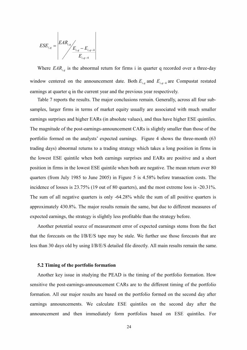
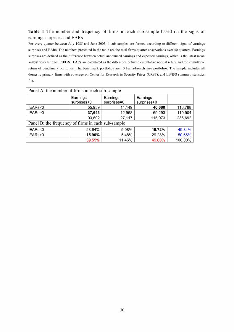
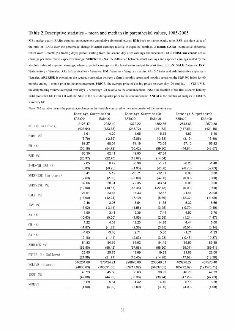
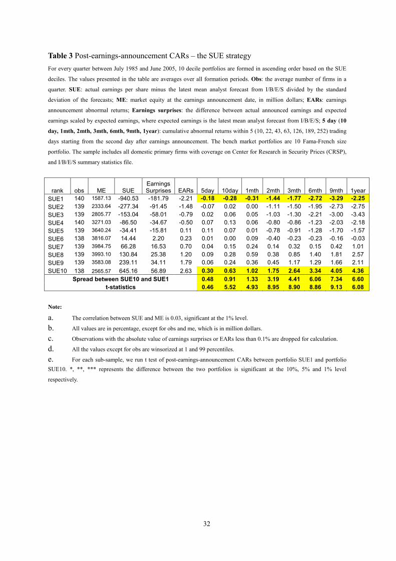
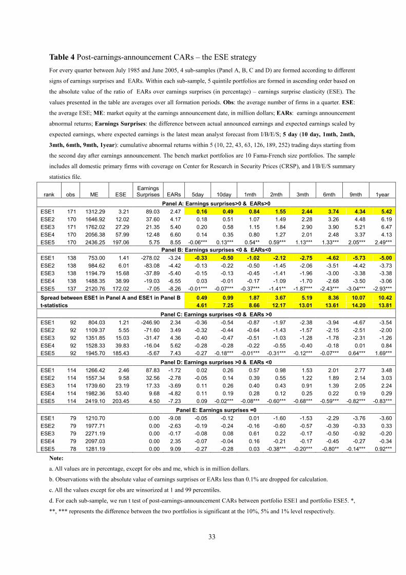
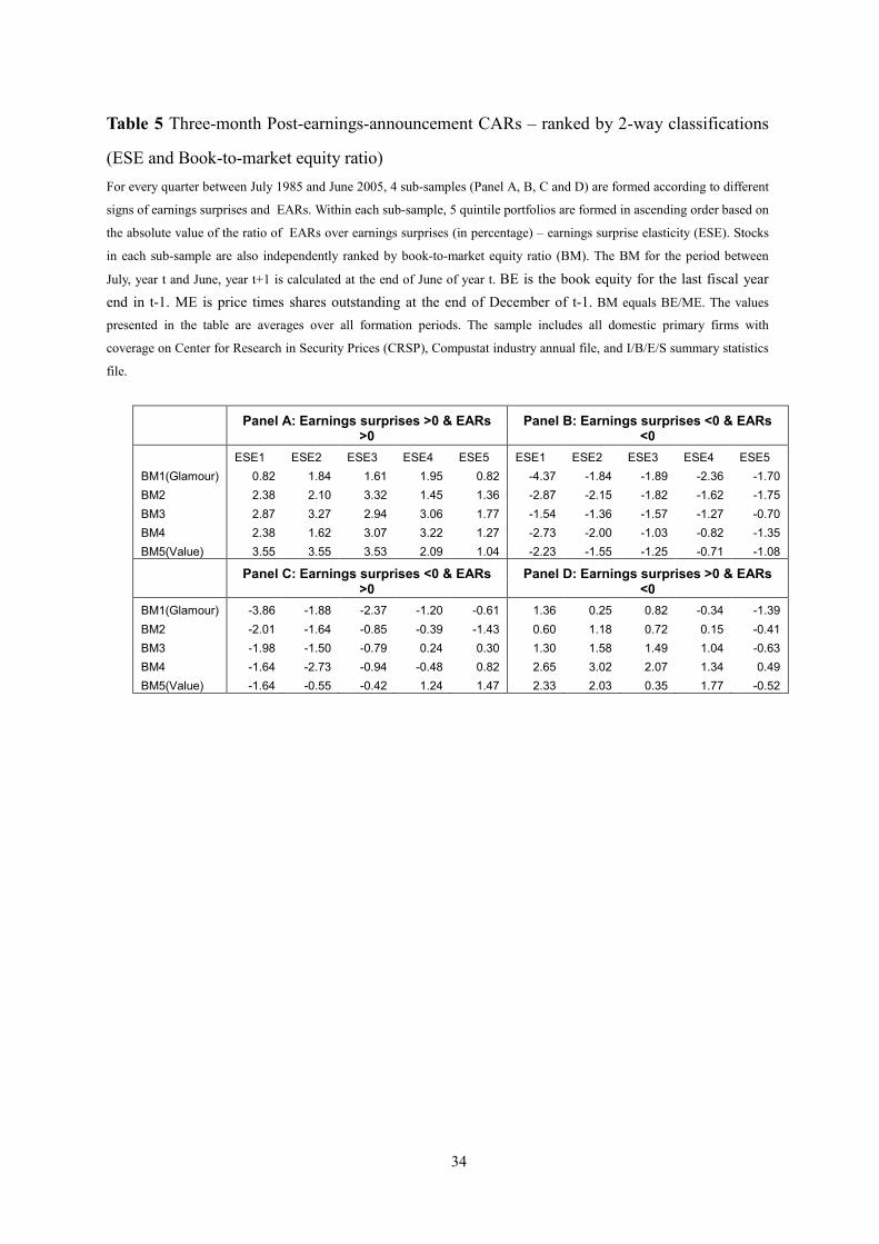
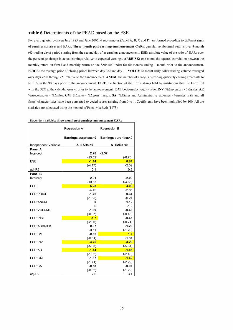
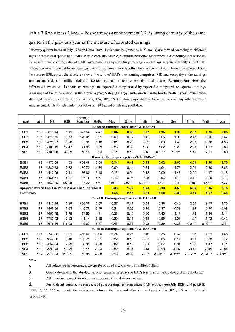
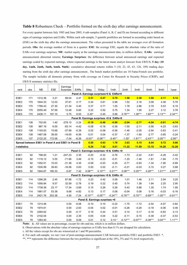
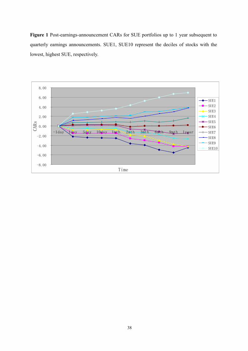
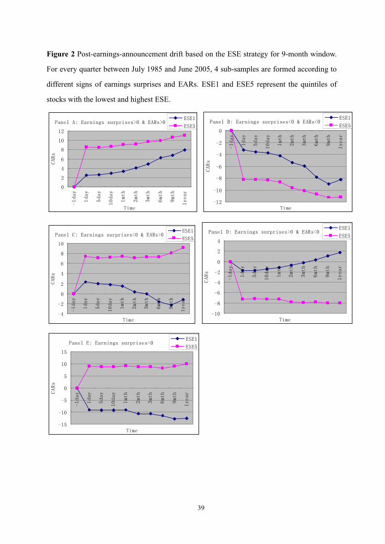
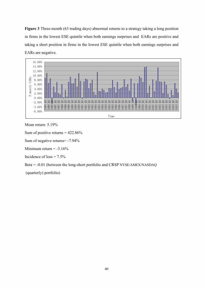
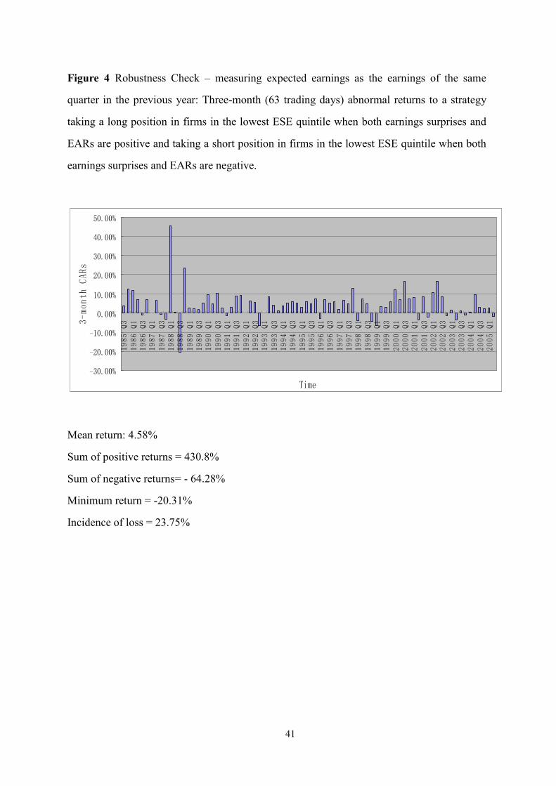
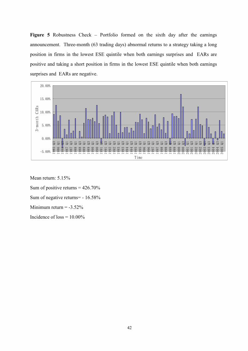