a new model for analyzing sociolinguistic variation: the interaction of
TRANSCRIPT
1
NEW MODEL FOR ANALYZING SOCIOLINGUISTIC VARIATION: THE INTERACTION OF SOCIAL AND LINGUISTIC CONSTRAINTS
By
RANIA HABIB
A DISSERTATION PRESENTED TO THE GRADUATE SCHOOL OF THE UNIVERSITY OF FLORIDA IN PARTIAL FULFILLMENT
OF THE REQUIREMENTS FOR THE DEGREE OF DOCTOR OF PHILOSOPHY
UNIVERSITY OF FLORIDA
2008

2
© 2008 Rania Habib

3
To my parents: Ibrahim and Amira
To my sister: Suzi To my brothers: Husam and Faraj
I love you ….
4
ACKNOWLEDGMENTS
This study owes a great deal to my adviser, Professor Fiona McLaughlin. Although I did
not take a course with her, I had a very nice experience working with her as a Research Assistant
in “The Project on the Languages of Urban Africa.” I admired her eloquence and personality
from the time I met her and when she attended one of our Research Methods class as a visiting
professor. In that class, Dr. McLaughlin shared her experience with us about collecting data in
Senegal in Africa as part of an introduction to Field Methods. She has been very kind and
listened closely whenever I felt hesitant towards making a decision. She has been supportive in
my job search and promoting my research and me among colleagues.
This study also owes a great deal to Professor Caroline Wiltshire who has helped me with
the Gradual Learning Algorithm (GLA). My interest in GLA started when I was taking Issues in
Phonology with her. Then, I wrote a paper for that class, using the idea of the GLA. This idea
extended to my study in greater depth. She has been caring and supportive from the time I came
to UF as a Fulbright student. I do not forget the time when I was very sick and she offered to take
me to the doctor and the time she sent me a wonderful report about my performance in my
classes and the professors’ evaluation of me.
I would like to thank Professor Atiqa Hachimi for being on my committee and for the
support and comments she has given me. I would also like to thank Professor Jessi Aaron for
agreeing to be on my committee as an external member at a short notice. Her comments have
been valuable. I would also like to thank Professor André Khuri for his help in statistics.
Unfortunately, uncontrollable circumstances prevented him from staying on my committee.
I would like to extend my thanks to all the faculty members at the Linguistics Department
who were part of my training in many fields and a window for widening my horizons. Many of
them have been very helpful and willing to discuss some questions regarding my study or were
5
very interested in my work and progress and supportive of my career development as well as the
promotion of my work among colleagues, such as Diana Boxer, Edith Kaan, Brent Henderson,
Wind Cowles, Ratree Wayland, and Eric Potsdam. I would also like to pass a note of thanks to
all my graduate friends and colleagues at the Linguistics Department, wishing them all the best
in their careers.
I would like to thank my international adviser, Debra Anderson, who has been like a
mother to me in the absence of my real mother. She has been a great companion when I needed
one. She listened and advised whenever she could. Thanks go to all my friends and those who
opened their hearts and homes to me here in Gainesville, FL and in the U.S. Everyone has
contributed in some way to my life.
My greatest appreciation goes to my parents who brought me to this world and have shown
support throughout my life. Their support has made me who I am. I hope you will always be
proud of me. To my sister, Suzi, and two brothers, Faraj and Husam, who have also shown me
great support, I want to say I am proud of you and of being your sister. I love you all so much.
Finally, I want to extend special thanks to all those who participated in this study. Without
you, it would not have been possible. I appreciate your enthusiasm to help and be part of my
work. I am grateful to you for the rest of my life.
6
TABLE OF CONTENTS page
ACKNOWLEDGMENTS ...............................................................................................................4
LIST OF TABLES .........................................................................................................................12
LIST OF FIGURES .......................................................................................................................16
LIST OF ABBREVIATIONS ........................................................................................................17
ABSTRACT ...................................................................................................................................18
CHAPTER
1 INTRODUCTION ..................................................................................................................21
1.1 Proposal ............................................................................................................................21 1.2 Correlation between Linguistic Variables and Social Factors in the Course of the
Development of Sociolinguistic Methodology ...................................................................30 1.2.1 Quantitative Methods .............................................................................................31 1.2.2 Long Term Participant Observation Methods ........................................................33
1.2.2.1 Participant observation (ethnography of communication) and quantitative analysis ..............................................................................................34
1.2.2.2 Participant observation and qualitative analysis ..........................................35 1.2.2.3 Participant observation and combining quantitative and qualitative
analyses .................................................................................................................37 1.2.3 Summary of the above Sociolinguistic Methods ....................................................39
1.3 Introduction to Optimality Theory (OT) ...........................................................................43 1.3.1 Constraint Demotion Algorithm (CDA), Floating Constraints (FCs), and
Stratified Grammars (SG) ............................................................................................45 1.3.1.1 Constraint Demotion Algorithm (CDA) ......................................................46 1.3.1.2 Floating Constraints (FCs) ...........................................................................46 1.3.1.3 Stratified Grammar (SG) ..............................................................................48
1.3.2 Working Mechanism and Advantages of the GLA over CDA, FCs, and SG ........49 1.3.2.1 Pure linguistic applications of the GLA .......................................................54 1.3.2.2 Example of a sociolinguistic application of GLA ........................................55 1.3.2.3 Concluding remarks about the GLA ............................................................58
1.4 Conclusion ........................................................................................................................59 1.5 Research Questions ...........................................................................................................61 1.6 Structure of the Study .......................................................................................................61
2 METHODOLOGY .................................................................................................................65
2.1 Setting: The City of Hims .................................................................................................65 2.2 Speech Sample ..................................................................................................................69 2.3 Variables under Investigation ...........................................................................................75
7
2.3.1 Linguistic Variables ................................................................................................75 2.3.1.1 The variable (q) ............................................................................................76
2.3.1.2 The variable () ............................................................................................77
2.3.1.3 The variable () ............................................................................................79 2.3.2 Social Variables ......................................................................................................80
2.3.2.1 Overview of Al-Hameeddieh .......................................................................81 2.3.2.2 Overview of Akrama ....................................................................................82
2.4 Analysis ............................................................................................................................83
3 THEORETICAL ANALYSIS ................................................................................................87
3.1 Introduction to the Theoretical Analysis of the Data ........................................................87
3.2 Modeling Variation between [q] and [] ..........................................................................88
3.2.1 Linguistic Constraints Pertinent to the Variation between [q] and [] ...................89 3.2.1.1 Grammar of RCA .........................................................................................91 3.2.1.2 Grammar of HCA .........................................................................................93 3.2.1.3 Acquisition of the HCA form by an RCA speaker .......................................94
3.2.2 Social Constraints Pertinent to the Variation between [q] and [] .......................101
3.2.3 Praat Analysis of the Variation between [q] and [] ............................................103
3.2.4 Concluding Remarks on the Sociolinguistic Variation between [q] and [] .128 3.3 Modeling Variation between [t] and [s] and between [d] and [z] ...................................130
3.3.1 Linguistic Constraints Pertinent to the Variation between [t] and [s] and [d] and [z] ........................................................................................................................135
3.3.2 Faithfulness and the Variants [t] and [s] and [d] and [z] ......................................136 3.3.3 Social Constraints Pertinent to the Variants [t] and [s] and [d] and [z] ...............140 3.3.4 Will Social Constraints Affect the Previous Results? ..........................................142
3.3.2.1 Concluding remarks on the stable variation among [t] and [s] and [d] and [z] .................................................................................................................144
4 QUANTITATIVE ANALYSES OF [q] VS. [] ..................................................................145
4.1 Introduction .....................................................................................................................145 4.2 Tests of Association of Social Class with Education, Income, Residential Area, and
Occupation ........................................................................................................................145 4.2.1 Test of Association between Social Class and Education ....................................147 4.2.2 Test of Association between Social Class and Income ........................................148 4.2.3 Test of Association between Social Class and Occupation ..................................149 4.2.4 Test of Association between Social Class and Residential Area .........................150 4.2.5 Concluding Remarks on the Tests of Association between Social Class and
Education, Income, Occupation, and Residential Area .............................................151
4.3. Speakers’ Distribution of [q] and [] .............................................................................153 4.3.1 Exploring the Type of Statistical Distribution among the Various Groups .........155 4.3.2 Bivariate Correlations Procedure between the Two Dependent Variants [q]
and [] ........................................................................................................................158
8
4.3.3 Generalized Linear Models (GZLM) Procedure for the Effect of the Four Independent Variables on the Two Dependent Variants [q] and [] .........................159
4.3.3.1 Negative binomial regression showing the main effects of the four independent variables, age, gender, residential area, and social class, on the variable use of the dependent variant [q] ............................................................161
4.3.3.2 Negative binomial regression showing the effect of the interaction of the independent variables, age, gender, and residential area, on the variable use of the dependent variant [q] ..........................................................................165
4.3.3.3 Negative binomial regression showing the effect of the interaction of the two independent variables, age and gender, on the variable use of the dependent variant [q] ..........................................................................................167
4.3.3.4 Negative binomial regression showing the main effects of the four independent variables, age, gender, residential area, and social class, on the variable use of the dependent variant [] ............................................................168
4.3.3.5 Negative binomial regression showing the effect of the interaction of the independent variables, age, gender, and residential area, on the variable use of the dependent variant [] ..........................................................................171
4.3.3.6 Negative binomial regression showing the effect of the interaction of the two independent variables, age and gender, on the variable use of the dependent variant [] ..........................................................................................172
4.4 Discussion of the Statistical Results ...............................................................................173 4.4.1 Age .......................................................................................................................173 4.4.2 Gender ..................................................................................................................177 4.4.3 Residential area ....................................................................................................180 4.4.4 Social class ...........................................................................................................182 4.4.5 Relationship of the Statistical Findings to the Theoretical Analysis ....................185
4.5 Frequency Effects on the Acquisition of [] ...................................................................188 4.6 Conclusion ......................................................................................................................192
5 QUANTITATIVE ANALYSIS OF THE VARIANTS [t] AND [s] AND [d] AND [z] ......200
5.1 Introduction .....................................................................................................................200 5.2 Analysis of the Use of [t] and [s] ....................................................................................200 5.3 Discussion of the Frequency Analysis of the Stable Variants [t] and [s] .......................206 5.4 Analysis of the Use of [d] and [z] ...................................................................................209 5.5 Discussion of the Frequency Analysis of the Stable Variants [d] and [z] ......................214 5.6 General Discussion .........................................................................................................216 5.7 Conclusion ......................................................................................................................222
6 CONCLUSION .....................................................................................................................224
6.1 Introduction .....................................................................................................................224 6.2 Use of OT and the GLA to Account for Switching between Two Different Dialects
and Inter- and Intra-speaker Variation ..............................................................................224 6.3 Incorporating Social Factors into the GLA ....................................................................226 6.4 Role Played by Social Factors ........................................................................................227
9
6.5 Consistency of Variation ................................................................................................228 6.6 Markedness Constraints versus Social Constraints ........................................................229 6.7 Advantages of and Caveats about the New Model .........................................................232
6.7.1 Advantages of the New Model .............................................................................232 6.7.2 Caveats about the New Model and Other Limitations of the Study .....................235
6.8 Frequency effects ............................................................................................................237 6.9 Implications, Directions and Recommendations for Future Research ...........................238 6.10 Conclusion ....................................................................................................................244
APPENDIX
A TESTS OF ASSOCIATION FOR SOCIAL CLASS WITH EDUCATION, INCOME, OCCUPATION, AND RESIDENTIAL AREA ...................................................................245
Cross Tabulations (Contingency Tables) ..............................................................................245 Social Class * Education ...............................................................................................245 Social Class * Income ...................................................................................................246 Social Class * Occupation .............................................................................................247 Social Class * Residential Area .....................................................................................248
B DESCRIPTIVE STATISTICS EXAMINING TYPE OF DISTRIBUTION IN THE DATA ...................................................................................................................................250
Gender ...................................................................................................................................250 qaf: Gender Histograms .................................................................................................254 qaf: Gender Boxplots .....................................................................................................255 hamza: Gender Histograms ...........................................................................................255 hamza: Gender Boxplots ...............................................................................................256
Age ........................................................................................................................................257 qaf: Age Histograms ......................................................................................................261 qaf: Age Boxplots ..........................................................................................................262 hamza: Age Histograms ................................................................................................263 hamza: Age Boxplots ....................................................................................................264
Area .......................................................................................................................................264 qaf: Area Histograms .....................................................................................................269 qaf: Area Boxplots .........................................................................................................270 hamza: Area Histograms ...............................................................................................270 hamza: Area Boxplots ...................................................................................................271
Social Class ...........................................................................................................................272 qaf: Social Class Histograms .........................................................................................276 qaf: Social Class Boxplots .............................................................................................277 hamza: Social Class Histograms ...................................................................................278 hamza: Social Class Boxplots .......................................................................................279
C GENERALIZED LINEAR MODELS RESULTS FOR THE DEPENDENT VARIABLE [q] ....................................................................................................................280

10
Poisson Loglinear Regression Showing the Main Effects of the Independent Variables, Age, Gender, Residential Area, and Social Class, on the Use of the Dependent Variant [q] .........................................................................................................................280
Negative Binomial Regression to Show the Main Effects of Gender, Age, Residential Area, And Social Class on the Use of [q] .........................................................................283
Estimated Marginal Means 1: Age ................................................................................286 Estimated Marginal Means 2: Gender ...........................................................................287 Estimated Marginal Means 3: Area ...............................................................................287 Estimated Marginal Means 4: Social Class ...................................................................288
Negative Binomial Regression Showing the Effect of the Interaction of Three Independent Variables, Age, Gender, and Residential Area, on the Use of the Dependent Variant [q] .......................................................................................................289
Negative Binomial Regression to Show the Effect of the Interaction of Gender and Age on the Use of [q] ................................................................................................................293
D GENERALIZED LINEAR MODELS RESULTS FOR THE DEPENDENT VARIABLE [] .....................................................................................................................297
Negative Binomial Regression to Show the Effect of Gender, Age, Residential Area, and Social Class on the Use of [] ....................................................................................297
Estimated Marginal Means 1: Age ................................................................................300 Estimated Marginal Means 2: Gender ...........................................................................300 Estimated Marginal Means 3: Area ...............................................................................301 Estimated Marginal Means 4: Social Class ...................................................................301
Negative Binomial Regression Showing the Effect of the Interaction of the Three Independent Variables, Age, Gender, and Residential Area on the Use of the Dependent Variant [] .......................................................................................................302
Negative Binomial Regression Showing the Effect of the Interaction of the Two Independent Variables, Age and Gender, on the Use of the Dependent Variant [] ........306
E GENERALIZED LINEAR MODELS THE DEPENDENT VARIABLES [q] AND [] ....310
Negative Binomial Regression Showing the Main Effects of Education, Income, and Occupation on the Variable Use of [q] .............................................................................310
Negative Binomial Regression Showing the Main Effects of Education, Income, and Occupation on the Variable Use of [] ..............................................................................313
F INTERNTIONAL PHONETIC ALPHABET (IPA) SYMBOLS FOR STANDARD ARABIC, HIMSI COLLOQUIAL ARABIC, AND RURAL COLLOQUIAL ARABIC ...317
Standard Arabic Phonemic System in IPA ...........................................................................317 Himsi Colloquial Arabic Phonemic System in IPA .............................................................317 Rural Colloquial Arabic Phonemic System in IPA ..............................................................318

11
LIST OF REFERENCES .............................................................................................................319
BIOGRAPHICAL SKETCH .......................................................................................................333
12
LIST OF TABLES
Table page 2-1. Distribution of study participants ...........................................................................................72
2-2. Variants of the variables (q), (), and () in the speech of non-migrant rural speakers, native Himsi speakers, and migrant rural speakers ............................................................75
3-1. Variants of the variable (q) in SA, HCA, and RCA ...............................................................89
3-2. Phonemic difference between HCA and RCA speakers ........................................................90
3-3. Ranking of RCA: Underlying form /qaraabi/ .........................................................................93
3-4. Ranking of RCA: Underlying form /alem/ ...........................................................................93
3-5. Ranking of HCA: Underlying form /araabi/ .........................................................................94
3-6. Acquisition of HCA form by RCA speaker: Underlying form /qaraabi/ ...............................97
3-7. Ranking values and disharmonies of *, *q, and IDENT-IO (RTR) ...................................107
3-8. Ranking values and disharmonies of *, *q, and IDENT-IO (RTR), manipulating the output distribution to 100% use of [q] and [] and 0% use of [] and [q] when the input has /q/ and // respectively ......................................................................................109
3-9. Ranking values and disharmonies of *, *q, and IDENT-IO (RTR), manipulating the values of the pair distribution to 18% [] and 82% [q] ....................................................110
3-10. Ranking values and disharmonies of *, *q, and IDENT-IO (RTR), manipulating the values of the pair distribution to 4% [] and 96% [q] ......................................................110
3-11. Ranking values and disharmonies of *, *q, and IDENT-IO (RTR), manipulating the values of the pair distribution to 98% [] and 2% [q] ......................................................111
3-12. Ranking values and disharmonies of *, *q, *F[q], and IDENT-IO (RTR), without manipulation of the values of the pair distribution ..........................................................114
3-13. Ranking values and disharmonies of *, *q, *F[q], and IDENT-IO (RTR), manipulating the values of the pair distribution to 65% [] and 35% [q] ........................116
3-14. Ranking values and disharmonies of *, *q, *F[q], *OLD[], and IDENT-IO (RTR), without manipulation of the values of the pair distribution .............................................117
13
3-15. Ranking values and disharmonies of *, *q, *F[q], *OLD[], and IDENT-IO (RTR), manipulating the values of the pair distribution to 37% [] and 63% [q] ........................118
3-16. Ranking values and disharmonies of *, *q, *F[q], *OLD[], *AKR[], and IDENT-IO (RTR), manipulating the values of the pair distribution to 18% [] and 82% [q] ...........119
3-17. Ranking values and disharmonies of *, *q, *F[q], *OLD[], *AKR[], and IDENT-IO (RTR), without manipulation of the values of the pair distribution ................................120
3-18. Ranking values and disharmonies of *, *q, *F[], *OLD[], *AKR[], and IDENT-IO (RTR), without manipulation of the values of the pair distribution ................................121
3-19. Ranking values and disharmonies of *, *q, *F[], *OLD[], *AKR[], and IDENT-IO (RTR), manipulating the values of the pair distribution to18% [] and 82% [q] ............121
3-20. Ranking values and disharmonies of *, *q, *M[], *OLD[], *AKR[], and IDENT-IO (RTR), manipulating of the values of the pair distribution to 4% [] and 96% [q] .........124
3-21. RCA input: Ranking values and disharmonies of *, *q, *F[q], *YOUNG[q], *HAM[q], and IDENT-IO (RTR), with manipulation of the values of pair distribution to 98% [] and 2% [q] ..................................................................................................................125
3-22. HCA input: Ranking values and disharmonies of *, *q, *F[q], *YOUNG[q], *HAM[q], and IDENT-IO (RTR), with manipulation of the values of pair distribution to 98% [] and 2% [q] ..................................................................................................................127
3-23. The variants of the variables () and () in SA, HCA, and RCA .......................................133
3-24. List of environments for [t] and [s] and [d] and [z] ............................................................134
3-25. Ranking values and disharmonies of *s, *t, and IDENT-IO (Manner), without manipulation of the values of the pair distribution ..........................................................137
3-26. Ranking values and disharmonies of *s, *t, and IDENT-IO (Manner) when ranked at 90, 90, 100 respectively ...................................................................................................137
3-27. Ranking of *s, *t, and IDENT-IO (Manner): Underlying form /ktiir/ ...............................138
3-28. Ranking of *s, *t, and IDENT-IO (Manner): Underlying form /masalan/ .........................138
3-29. Ranking values and disharmonies of *s, *t, and IDENT-IO (Manner), manipulating the pair distribution to 100% use of [ktiir] and 100% use of [masalan] ................................138
3-30. Ranking values and disharmonies of *s, *t, and IDENT-IO (Manner) with manipulation of the pair distribution to 100% use of [ktiir] ............................................139
14
3-31. Ranking values and disharmonies of *s, *t, IDENT-IO (Manner), *F[t], and *F[s] without manipulation of the values of the pair distribution .............................................143
3-32. Ranking values and disharmonies of *s, *t, IDENT-IO (Manner), *F[t], and *F[s], manipulating the values of the pair distribution to 100% use of both [ktiir] and [masalan] ..........................................................................................................................143
4-1. Distribution of [q] and [] in the speech of each speaker .....................................................154
4-2. Bivariate correlations between the dependent scale variants [q] and [] .............................158
4-3. Distribution of [q] and [] according to age group ...............................................................174
4-4. Distribution of [q] and [] according to gender ....................................................................177
4-5. Variability in the speech of Speaker-20 ...............................................................................179
4-6. Distribution of [q] and [] according to age and gender .......................................................180
4-7. Distribution of [q] and [] according to age and gender without speakers 29, 30, & 31 .....180
4-8. Distribution of [q] and [] according to residential area ......................................................181
4-9. Distribution of [q] and [] according to age and residential area .........................................182
4-10. Distribution of [q] and [] according to social class ...........................................................183
4-11. Most frequent words produced with [q] and [] .................................................................194
4-12. Percentage of the occurrence of frequently occurring words in the speech of varying speakers ............................................................................................................................196
5-1. Most frequent words produced with [t] and [s] ....................................................................202
5-2. Contingency table showing the frequency use of [t] and [s] words and their conditional distribution in all speakers ...............................................................................................204
5-3. Two tailed One-Sample T-Test comparing the significance of the difference in the frequency of [t]-words and [s] words ...............................................................................206
5-4. Similarity between the vowel system of observed words with [s] with their counterparts in SA ................................................................................................................................208
5-5. Assimilated words with [s] to the vowel system of the dialects ...........................................208
5-6. Most frequent words produced with [d] and [z] ...................................................................210
15
5-7. Contingency table showing the frequency use of [d] and [z] words in all speakers ............212
5-8. Two tailed One-Sample T-Test comparing the significance of the difference in the frequency of [d]-words and [z]-words .............................................................................214
5-9. Similarity between the vowel system of observed words with [z] with their counterparts in SA ................................................................................................................................216
5-10. Assimilated words with [s] to the vowel system of the dialects .........................................216
16
LIST OF FIGURES
Figure page 1-1. Categorical Ranking ...............................................................................................................50
1-2. Free Ranking...........................................................................................................................50
1-3. C2 >> C1 ..................................................................................................................................50
1-4. C1 >> C2 ..................................................................................................................................51
2-1. Map of Syria and neighboring countries. ...............................................................................67
2-2. City Plan of Hims. Adopted from the Homs City Council (2008). I point to the areas of concern in this study and give their name in English, as a point of reference. ..................86
3-1. Ranking of RCA .....................................................................................................................98
3-2. Ranking of HCA form ...........................................................................................................99
3-3. Ranking of the three constraints IDENT-IO (RTR), * and *q in an oscillating speaker ......100
4-1. Bar chart for the distribution of the six educational groups between lower-middle and upper-middle classes ........................................................................................................148
4-2. Bar chart for the distribution of the three income groups between lower-middle and upper-middle classes ........................................................................................................149
4-3. Bar chart for the distribution of the four occupational groups between lower-middle and upper-middle classes ........................................................................................................150
4-4. Bar chart for the distribution of the lower-middle and upper-middle classes in the two residential areas: Akrama and Al-Hameeddieh ...............................................................151
4-5. Histogram showing the skewness to the left in the females’ use of [q] ...............................157
5-1. Distribution of [t]-words between high and low frequency .................................................205
5-2. Distribution of [s]-words between high and low frequency .................................................205
5-3. The distribution of [d]-words between high and low frequency ..........................................213
5-4. The distribution of [z]-words between high and low frequency ..........................................213
17
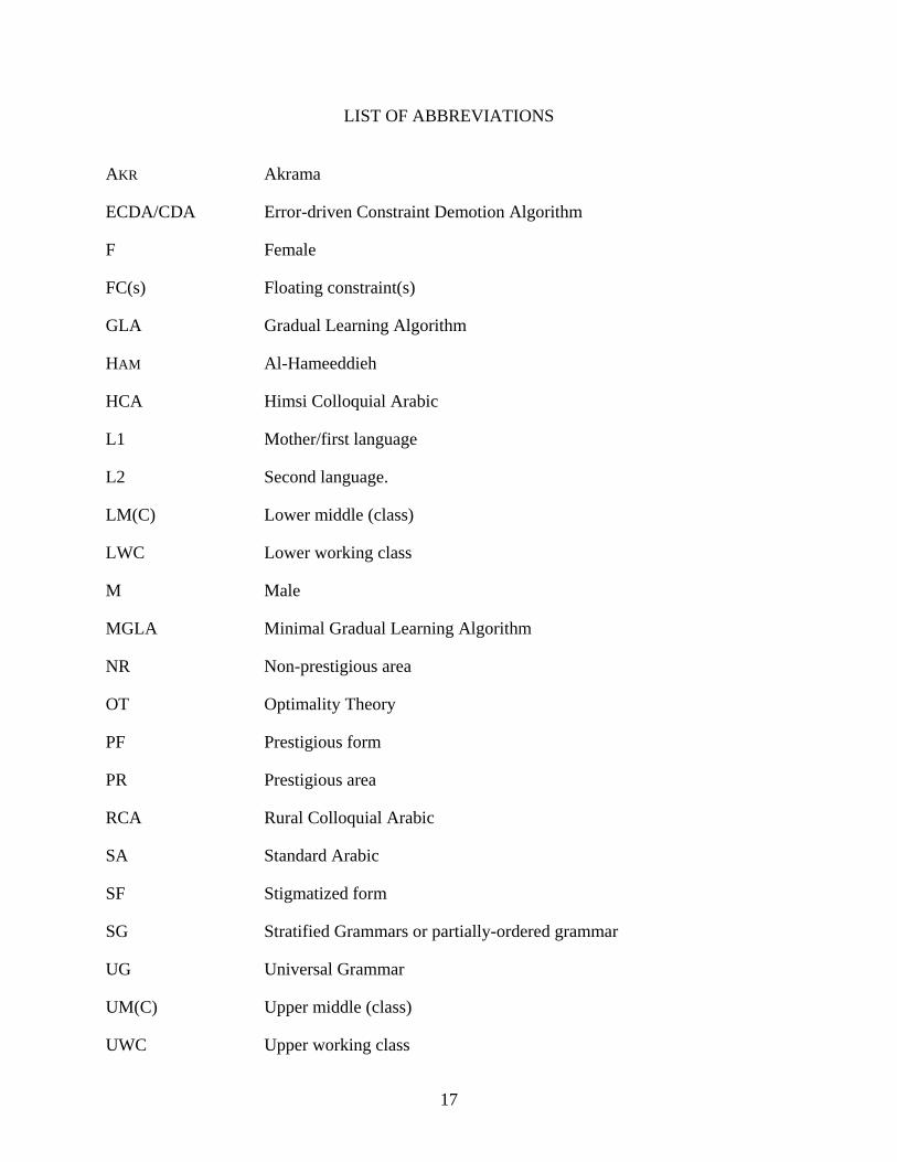
LIST OF ABBREVIATIONS
AKR Akrama
ECDA/CDA Error-driven Constraint Demotion Algorithm
F Female
FC(s) Floating constraint(s)
GLA Gradual Learning Algorithm
HAM Al-Hameeddieh
HCA Himsi Colloquial Arabic
L1 Mother/first language
L2 Second language.
LM(C) Lower middle (class)
LWC Lower working class
M Male
MGLA Minimal Gradual Learning Algorithm
NR Non-prestigious area
OT Optimality Theory
PF Prestigious form
PR Prestigious area
RCA Rural Colloquial Arabic
SA Standard Arabic
SF Stigmatized form
SG Stratified Grammars or partially-ordered grammar
UG Universal Grammar
UM(C) Upper middle (class)
UWC Upper working class
18
Abstract of Dissertation Presented to the Graduate School of the University of Florida in Partial Fulfillment of the Requirements for the Degree of Doctor of Philosophy
NEW MODEL FOR ANALYZING SOCIOLINGUISTIC VARIATION: THE INTERACTION OF SOCIAL AND LINGUISTIC CONSTRAINTS
By
Rania Habib
August 2008
Chair: Fiona Mc Laughlin Cochair: Caroline Wiltshire Major: Linguistics
In this study, I present a new model for analyzing sociolinguistic variation within the
framework of Optimality Theory (OT) and the Gradual Learning Algorithm (GLA). This model
contributes to the advancement of sociolinguistic methodology as well as to OT and the GLA,
unifying both linguistic and social factors. I propose a number of social constraints and
incorporate them with linguistic constraints in the GLA. I show that incorporating social
constraints yields variant-usage percentages that match real life occurrences. I follow the
evaluation process of stochastic grammar in which social constraints are treated like linguistic
constraints on a continuous scale of ranking strictness. Their ranking values may differ from one
speaker or group of speakers to another. These differences in the ranking values may result in
intra- and inter-speaker, intra- and inter-group, intra- and inter-community, or intra- and inter-
dialect variation. The number and type of social constraints involved influence the percentage of
occurrence of each variant and affect the ranking values of other constraints and the grammar
chosen by a speaker or a group of speakers at a particular time and place.
This model enables us to show the effect of linguistic and social constraints
simultaneously. It allows us to investigate individual as well as group grammars and shows that
19
those grammars may act independently from each other. It also enables us to project expected
percentages of variation by manipulating either the ranking values of constraints or the pair
distribution of the output. Evidence comes from the study of the naturally occurring speech of
migrant rural speakers of Colloquial Arabic to the city of Hims, Syria. These speakers show
different degrees of variation, particularly regarding the use of the two variants [q] and [], based
on various social factors, such as age, gender, residential area, and social class.
The aim of the study is to show how rural migrants adopt the new phonological system of
the urban dialect to appear prestigious. The study will focus on the sound change of [q] to [] and
the four stable variants [t] and [s] and [d] and [z]. It will show that variation may be influenced
by different factors. The variable use of [q] and [] is attributed to prestige and social factors.
The use of [t] and [s] and [d] and [z] is not social in nature; it has developed historically from the
Standard Arabic (SA) [] and [] respectively as a response to markedness constraints. Today,
this variation is stable and each of the four variants is used in specific lexical items. Faithfulness
constraints play a major role in maintaining the pronunciation of the input as [t] and [s] and [d]
and [z] in the output. This stable phenomenon is further explained in terms of the two opposing
effects of frequency (Bybee 2001).
In a situation where prestige plays a role in adopting a new variant, as in the case of rural
migrants to the city of Hims, social constraints are viewed as the motivating force behind
changing a grammar at a particular time and place. However, one should take into account that
the activation of social constraints depends on the speaker’s selection or choice to activate them
or not. Hence, these constraints may rank very high in the speech of a speaker who is highly
aware of the social values attached to a certain sound. On the other hand, they may rank very low
in the speech of a person who, for example, does not care to adopt a new form.

20
A theory that can take into account all the factors that lead to variation is a better theory
than one that takes into account social factors in isolation and ignores grammatical factors or
vice versa. Integrating social constraints into formal theory and showing that social constraints
can have equal weight or even more weight than grammatical constraints in conditioning
variation and change is essential in this study. Including social constraints in the computation
provides explanation of the observed sociolinguistic variation between [q] and [] among
members of the same social group or among different speakers or social groups. Interacting
social constraints with linguistic constraints in the same framework is a simple comprehensive
method to depict and explain the mental process of a speaker at a certain time and/or place.
Feeding the GLA with the right output distribution gives the specific ranking values or grammar
of each speaker or group of speakers. In other words, the model takes advantage of the stochastic
grammar embedded in the GLA to generate grammars that match real life output percentages
without trying all the possible rankings of constraints and counting the times those rankings give
a certain output. Furthermore, where a statistical analysis fails to indicate the interaction between
one social factor and others, the specificity implemented in the GLA by dividing a social factor
into a number of social constraints enables us to see interaction among the same social
constraints that emerged as insignificant in the statistical analysis. In this sense, implementing
social factors as constraints and accounting for sociolinguistic variation within the framework of
OT and the GLA has an advantage over other theories.
21
CHAPTER 1 INTRODUCTION
1.1 Proposal
In this study, I present a new model for analyzing sociolinguistic variation, employing
Optimality Theory (OT) (Prince and Smolensky 2004 [1993]) and the Gradual Learning
Algorithm (GLA) (Boersma and Hayes 2001). This model contributes to the advancement of
sociolinguistic methodology as well as to OT and the GLA, unifying both linguistic and social
factors. I propose a number of social constraints and incorporate them into the GLA, where they
intersect with linguistic constraints, and show that incorporating social constraints with linguistic
constraints in the GLA yields results that reflect real life performances. Introducing social
constraints, for the first time, as integral part of linguistic theory could be considered an
advancement to OT and the GLA, which so far dealt only with linguistic constraints. As the GLA
is based on continuous ranking and stochastic constraints, these social constraints will be treated
as continuous constraints whose ranking values differ from one speaker to another, from one
group of speakers to another, and from one community to another. These differences in the
ranking values may result in inter-speaker, intra- and inter-group, intra- and inter-community, or
intra- and inter-dialect variation. These ranking values may even differ within the same speaker
yielding intra-speaker variation. The number and type of social constraints involved influence
the percentage of occurrence of each variant and affect the weight of other constraints and the
grammar chosen by a speaker or a group of speakers at a particular time and place.
This model enables us to show the effect of linguistic and social constraints
simultaneously. It gives a mental representation of the grammatical process that takes place in
the speaker’s mind as a result of the integration of social and linguistic constraints. It allows us to
investigate individual as well as group grammars and shows that those grammars may act
22
independently from each other. In this sense, the model allows us to see that certain social
constraints, for example, may be activated by a certain speaker, but not others, and by one group
of speakers or more, but not others. Thus, in the same way that linguistic constraints have their
language specific ranking, social constraints maintain their relativity and specificity in the
particularity of the individual grammars and constraint rankings of individual speakers or groups
of speakers. The model also enables us to project expected percentages of variation by
manipulating the weight of the various constraints or the output pair distribution. Interestingly
enough, when constraints are set at an initial equal ranking value, the addition of one or more
social constraint(s) changes the ranking value of other constraints and gives us predictions on
what variation will look like if those social constraints are involved. Certain social constraints
give us expectations on what the speech of a particular speaker or group of speakers should
sound like. Furthermore, feeding the GLA with the right output distribution generates grammars
that match real life output percentages of each speaker or group of speakers without trying all the
possible rankings of constraints and counting the number of rankings that give each output.
Evidence comes from the study of the naturally occurring speech of migrant rural speakers of
Colloquial Arabic to the city of Hims, Syria. These speakers show different degrees of variation,
particularly regarding the use of the two variants [q] and [], based on various social factors,
such as age, gender, residential area, and social class. Their variation may also depend on the
interlocutor: a family member or a stranger.
The ability of the model to give a mental representation of what goes on in the speaker’s
mind and the conscious choice of a ranking value at a certain time and place endow the model
and the proposed linguistic and social constraints with psychological reality. The psychological
reality of grammars is a broad issue that is hard to determine or support completely. The idea of
23
the psychological reality of rules and representations goes back to Chomsky. However, many
expressed skepticism about Chomsky’s (1980) argument that rules and representations are part of
a grammar and a mental process (i.e., rules are psychologically real). Devitt (2006a), for
example, is skeptic of rules and principles and believes that they are not psychologically real.
Devitt (2006b) believes that there is only a “linguistic reality” that is mainly associated with
what is produced (whether spoken, signed, or written) (i.e., “the real subject matter of grammars”
(Slezak 2007)). Devitt’s (2006a) objection to Chomsky’s view of the psychological reality of
grammars as mental representations was critiqued by Slezak (2007) who observed that the
difference between Devitt’s view and Chomsky’s is merely terminological. Furthermore, Aske
(1990), in testing the psychological reality of Spanish stress rules, arrived at results that
contradict the traditional idea of the mental representation of rules (i.e., rules are not
psychologically real). Rather speakers access their lexicon when assigning stress to new words
they never heard before. They assign stress by analogy to existent patterns in the brain/lexicon.
Thus, patterns, not rules, are mentally represented. Similarly, Bybee and McClelland (2005)
argue against rule-based systems and the mental representation of rules in support of exemplar
models and connectionist models. They adopt the view that “specific experiences” have an
impact “on the mental organization and representation of language” (p. 381). For them,
language use has a major impact on language structure. The experience that users have with language shapes cognitive representations, which are built up through the application of general principles of human cognition to linguistic input. The structure that appears to underlie language use reflects the operation of these principles as they shape how individual speakers and hearers represent form and meaning and adapt these forms and meanings as they speak. (p. 382)
Bybee and McClelland’s view does not eliminate a cognitive representation of some kind
of form and meaning that are influenced by language use rather than by innate universal rules. In
this sense, language use may influence the mental representation of language. This view is not
24
very far apart from the influence that social factors could exert on the mental representation of
language in a sociolinguistic variation situation. In a sociolinguistic contact situation, speakers
are most likely aware of a linguistic change around them. For example, the Casablancan dialect,
which developed because of the extensive contact between different regional dialects of migrants
from rural and urban areas, was described towards the end of the twentieth century as an
“interdialect” that has psychological reality for Moroccans (Moumine 1990, cited in Hachimi
2007). Furthermore, Milroy (2006:151) espouses the view that “linguistic change is a process”
and some aspects of this process are “related to social factors”. For Milroy, language cannot
change on its own. It is a social phenomenon that involves a speaker and a listener. There is a
distinction between speaker innovation and linguistic change. Social factors constitute part of
any type of linguistic change because even internal changes involve production on the part of the
speaker and perception on the part of the listener. If we take Milroy’s argument into
consideration, we can conclude that in a sociolinguistic variation situation, people are aware of
the linguistic changes surrounding them and are most likely involved in them.
Returning to my initial assumption that the model and constrains proposed in this study are
psychologically real, I add that the speaker’s awareness of the social significance of a sound and
the change of the ranking values of constraints to sound prestigious involves learnability of new
ranking values. Learnability is usually associated with some mental grammatical processes. This
idea may contradict with Rumelhart and McClelland’s (1987) idea that learnability and language
use do not involve rules because of the probabilistic nature of natural language and the
variability in language use. However, I argue that variability in language use could be the result
of external factors that influence the choice of one ranking value over another. Choice is related
to consciousness (of grammatical processes and the likes), and thus has some mental realization
25
and psychological understanding of what is going on in a social situation in which a speaker
switches from one form to another and is noticed by listeners. In support of this view, I present
Cutillas-Espinosa’s (2004) view that a speaker can control the ranking values of his/her grammar
consciously (Section 1.3.2.2). For him, variation is not mechanical or automatic; rather, it is
based on personal conscious choices. In this way, Cutillas-Espinosa opposes the Neogrammarian
view that change is mechanical and automatic. Many researchers have argued, however, that
repetition and frequency may lead to the automatization of words and sequences of words (e.g.
Bybee 2001, 2003). That is, words or sequences of words form chunks in the brain and become
entrenched in their own representation and thus easier to access and use. This automatization is
applied also to social identity and information about the interlocutor and social settings. In other
words, speakers access this stored information along with the form or structure suitable for the
social setting or situation. Labov (1994:604), on the other hand, supports the Neogrammarian
view that language change is mechanical and automatic when it is “outside the range of
conscious recognition and choice.” In this way, any conscious attempt to change language is
subject to “higher-level stylistic options” or adherence to social factors and pressures. In this
sense, sociolinguistic change is mainly conscious and involves choice. Whether this change
becomes automatic or not later on in life is beyond the scope of this study and is worth
investigating in further research. However, it is noteworthy that for a sound change to be
considered automatic, it should not be the “goal of anyone at any time” (Boersma 1997b:2).
Since the change from [q] to [] is driven by prestige, it is teleological, and thus follows a
conscious process at least in the initial stages of learnability of the new prestigious form []. In
addition, the stigma that is associated with the rural form [q] encourages its users to abandon it
and adopt the prestigious form instead. Stereotype variables such as (q) which are avoided by

26
their own native speakers are indicative of the social awareness of them and their stigma as well
as of the prestige of the form those speakers switch to, in our case [].
Moreover, the social awareness that leads to learnability of new ranking values of
constraints provides evidence of the speaker’s consciousness of those constraints and the process
that accompanies them, not only in him/herself but also in other speakers or interlocutors who
tend to switch to a different sound or dialect or maintain his/her native sounds or dialect. A rural
migrant speaker to the city of Hims, for example, is aware of the accommodation to the Himsi
prestigious form, []. This awareness is expressed by many speakers in the recorded
conversations. Those speakers notice their own shift as well as the shift of others towards the use
of [] with strangers or non-family members. A number of speakers mentioned their observations
of other speakers changing their speech and using [] instead of [q] outside the family sphere
(Habib 2005, Sections 5.2 and 5.3). This awareness reflects on the psychological reality of the
different grammars and ranking values of constraints in each individual or group of individuals.
Awareness of such grammatical change in the other is a further reflection on the psychological
reality of the model and constraints. What makes this model interesting is that it does not
separate the social reality of language from the psychological reality of language. It integrates
both realities in the same framework, presenting the external influence on language as part of a
speaker’s internal process to sound externally prestigious.
The aim of the study is to show how rural migrants adopt the new phonological system of
the urban dialect to appear prestigious. The study will focus on the sound change of [q] to []; []
to [d], [z], or []; and [] to [t], [s], or []. It will show that variation may be influenced by
different factors. Variation in the use of [q] and [] is attributed to prestige and social factors.
27
Variation in the use of [d] and [z] and [t] and [s] is not social in nature; it has probably developed
historically as a response to markedness constraints. Today, this variation is stable and each of
the four variants is used in specific lexical items. Consequently, the underlying form of these
four variants is /d/ and /z/ and /t/ and /s/ respectively. Faithfulness constraints play the major role
in maintaining the pronunciation of the input as [d] and [z] and [t] and [s] in the output to
preserve the specificity observed in lexical items, in that each variant is designated a particular
phoneme with its correspondent allophone. Thus, the historical development led to the
disappearance of // and // from the phonemic system of speakers; they rarely appear as [] and
[] in colloquial speech. If they do, they appear as lexical borrowings from SA. Even then, they
may appear as [z] and [s] respectively. This is further attributed to markedness.
In a situation where prestige plays a role in adopting a new variant, as in the case of rural
migrants to the city of Hims, I view social factors as constraints that were inactive when the
speaker was living in his/her hometown. When this speaker moves to the city, s/he starts
activating those social constraints in addition to linguistic constraints based on positive evidence
or negative comments that s/he may hear from city people. The situation is analogous to a child
who is born with no previous knowledge of his/her mother tongue and based on positive
evidence, s/he starts activating the appropriate constraints and changing the ranking of those
constraints as s/he receives more input (e.g., Demuth 1995; Gnanadesikan 1995; Smolensky
1996). The difference between a child and an adult is that the child is not yet influenced by
society and social factors. In the case of the adult, social factors, such as prestige, societal
attitude, age, gender, social class, residential area, education, occupation, and social networks
potentially influence linguistic performance. Thus, I view social constraints as the motivating
force behind changing a grammar at a particular time and place. In this sense, the two types of

28
constraints – linguistic and social – interact to arrive at the desired result. However, one should
take into account that the activation of social constraints depends on the speaker’s selection or
choice to activate them or not. If the speaker chooses not to activate them or to activate just some
of them, s/he may continue to use his/her mother dialect or rather vary his/her speech, resulting
in intra- and inter-speaker variation. Many researchers emphasize the role of social factors in
affecting a change (e.g., Labov, 1963, 1966, 1972a, 2001; Trudgill 1974; Milroy 1980; Eckert
1991a; Haeri 1996). For example, Labov (2001:498) emphasizes that social factors are “the
forces that move and motivate change, and are responsible for incrementation and transmission
across generations.” Since social constraints can be the impetus for grammatical change, then we
can assume that they can play a major role in intra- and inter-speaker variation. Hence, these
constraints may rank very high in the speech of a speaker who is highly aware of the social
values attached to a certain sound. On the other hand, they may rank very low in the speech of a
person who, for example, does not care to adopt a new form or is too old to think about changing
his/her speech or his/her identity for this matter. Cases such as these have been observed in some
studies, such as Labov’s study of Martha’s Vineyard (1963). In Martha’s Vineyard, the Chilmark
fishermen, for example, showed strong defiance to forms from the mainland of New England;
they clung to the island’s old ways of pronouncing (ay) and (aw). That is, they maintained the
island’s centralized features. The younger age group also showed more centralization than most
age groups to show strong identification with the island and to distinguish themselves from the
summer tourists who come from the mainland. In addition, situations in which linguistic
behavior differs with age are very common. For instance, Miller (2005) found that there is a
great difference of accommodation to the Cairene forms between the first generation migrants to
Cairo and the second generation migrants who were born in Cairo. The second generation shows
29
complete accommodation to the Cairene forms, whereas the first generation migrants show
variation in their accommodation to the new forms. Furthermore, since those social constraints
will be considered on a continuous scale, they may lead to variation even within the same person,
leading to oscillation in the choice between two variants in the same conversation regardless of
the interlocutor. In this case, the speaker is trying to adjust his/her social constraints to fit in the
community. At the same time, s/he is also trying to adjust her/his grammatical constraints to fit
the social requirement. The result is that the speaker is probably confused and is unable to have a
good grip on one particular grammar and s/he will continue to oscillate in selecting different
ranking values and rankings for the various constraints.
Consequently, a theory that can take into account all the factors that lead to variation is a
better theory than one that takes into account social factors in isolation and ignores grammatical
factors or vice versa. Integrating social constraints into formal theory and showing that social
constraints can have equal weight or even more weight than grammatical constraints in
conditioning variation and change is an important development in this study. Including social
constraints in the computation provides explanation of the observed sociolinguistic variation
between [q] and [] among members of the same social group or among different speakers or
groups of speakers. Interacting social constraints with linguistic constraints in the same
framework is a simple comprehensive method to depict and explain the grammatical mental
process that takes place in the mind of a speaker at a certain time and/or place. Furthermore,
where a statistical analysis fails to indicate the interaction between one social factor and others,
the specificity implemented in the GLA by dividing a social factor into a number of social
constraints enables us to see interaction among the same social constraints that emerged as
insignificant in the statistical analysis. In this sense, combining OT and the GLA and including
30
social constraints in the computation have an advantage over other theories in accounting for
sociolinguistic variation and change. Traditional generative phonology manipulated grammatical
rules to deal with variation, which have their problems (Section 1.3). Traditional OT only
manipulated the rankings of linguistic constraints to analyze variation (e.g., Kochetov 1998 on
variation among four Polish dialects; Morris 2000 on variation among three Spanish varieties).
Sociolinguistic methods of analyzing linguistic variation focused on correlations between social
factors and linguistic variables with more emphasis on the development of methods of data
collection. In Section 1.2, I will give a brief background on the sequential development of
sociolinguistic methodology before presenting my model to allow the reader to compare my
model with previous ones.
1.2 Correlation between Linguistic Variables and Social Factors in the Course of the Development of Sociolinguistic Methodology
Since the mid 1960s and with the foundation of sociolinguistics by William Labov, social
factors started to gain importance in the field of linguistics and to play an important role in
analyzing and modeling speech. In Sociolinguistic Patterns (1972a:163), Labov stresses that
“[t]he process of sound change is not an autonomous movement within the confines of a
linguistic system, but rather a complex response to many aspects of human behavior.” Further,
in Principles of Linguistic Change (1994:1), Labov asserts that “[t]he separation of ‘internal’
from ‘external,’ ‘linguistic factors’ from ‘social factors’ may not seem practical to those who
view language as a unified whole where tout se tient, or those who believe that every feature of
language has a social aspect.” Throughout decades of sociolinguistic studies of variation, a great
shift in views took place, a shift from viewing language as reflection of the social to viewing
language as creator of the social (Rickford and Eckert 2001). The shift starts with Labov’s (1966,
1972a; Trudgill 1974) view of style variation as different levels of attention paid to speech and
31
ends with the constructivists’ view of the use of style to project a self-image and to construct
identity and social meaning (e.g., Eckert 1991b; Coupland 1985, 2001; Shilling-Estes 1999,
2002; Cameron 1998). Other views were also formed, such as Bell’s (1984, 1991) model of
‘audience design’ in which a speaker’s style is seen as a response to an audience. Bell viewed
style as a reflection of social variation, whereas Finegan and Biber (1994) viewed social
variation as a reflection of style. This is not to mention accommodation theory (Giles and
Powesland 1975; Giles, Coupland and Coupland 1991) which draws on the speaker’s orientation
and attitude to the interlocutor and on the role of identity (Coupland 1980) in determining
speakers’ style and their perception of style. In recent formal models, stylistic variation is
starting to be viewed as gradual, not abrupt (Boersma and Hayes 2001); it involves optionality
and learnability.
1.2.1 Quantitative Methods
Linguistic and stylistic variation was mainly measured by correlating various social factors
with the production of a certain linguistic variant in a particular way. Being the founding rock of
sociolinguistics, Labov’s quantitative methods of data analyses and modeling have influenced
many Arabic sociolinguists (e.g., Abd-el-Jawad 1981; Holes 1986; Walters 1989; Haeri 1991;
Abu-Haidar 1992; Daher 1998; Habib 2005). In his study of New York City (r) (1966, 1972a),
Labov correlated a number of social factors – age, sex, social class – with the pronunciation of
postvocalic r as (r-1) or (r-0)1, using various statistical methods. To examine the social
stratification of (r) in the speech of New Yorkers, Labov conducted a rapid and anonymous
survey to avoid the observer’s paradox. He selected three department stores in three different
locations in Manhattan, which are socially stratified: Saks Fifth Avenue (a high-status store with
1 (r-1) stands for r-full or the pronunciation of the variable (r) as [r]; (r-0) refers to the deletion of the variable (r) in pronunciation, that is it is realized as null or not realized at all, [Ø].
32
high prices), Macy’s (middle-class with middle prices), and Klein’s (a store with cheaper prices
for less affluent customers). In order to show that his hypothesis is general, he chose one
occupational group, salespeople, to show that social differences occur even within the same
occupational group, based on the status of the store and the customers. His prediction that the use
of (r-1) is socially stratified was confirmed. Saks’ employees used (r-1) sixty percent; Macy’s
employees fifty one percent; and Klein’s employees twenty percent. However, in the more
deliberate answer, all groups showed an increase in (r-1). What was striking is that the middle-
class store showed the highest degree of increase, which was attributed to hypercorrection among
the middle class. The study showed minor differences between men’s and women’s linguistic
behavior. There was also no strong correlation with age. While the younger generation in Saks
showed higher use of (r-1), the same was not observed in Macy’s and Klein’s. Rather, the
middle-aged group of the lower-middle class showed hypercorrection; it used more (r-1) than the
upper class, which is a sign of ‘linguistic insecurity’ (Labov 1972a, 2001). This survey was the
starting point for a larger project, expanding to the Lower East Side of New York, in which the
findings were no different.
In the Lower East Side of New York study (1972a), Labov sought to gather a more
representative sample of the city than its salespeople, using extensive interviews. He used a ten-
point scale to classify the various social classes. Labov assigned 0-1 for lower working-class
(LWC), 2-4 for upper working-class (UWC), 5-8 for lower middle-class (LMC), and 9 for upper
middle-class (UMC). In Labov’s study, the division among social classes was most evident
concerning the variable (th) that is realized as [], [t], and [t]. The latter is the most stigmatized
form and the most common among the LWC, whereas [] emerged as the most common among
the UMC. This is evident in the increase in the use of [] with the shift of style from casual
33
speech to word lists. The (r) variable showed similar results, but slightly smaller division among
social classes. There was also increase in the use of (r-1) in the speech of participants along the
style shift towards the most formal or minimal pairs. In this study, Labov used the “matched
guise” technique that was developed by Wallace Lambert (Lambert, Hodgson, and Fillenbaum
1960), which is a subjective reaction test, in order to see if all social classes evaluated the (r-1) in
the same way and whether New York City constitutes a speech community. Participants were
asked to listen to a tape, containing 24 sentences from five female readers. The same reader
pronounced the same sentence twice: once with [r] and once without it, but listeners were not
aware that the same speaker had said both utterances because sentences were randomized.
Participants were asked to judge the readers on a scale of occupational suitability (i.e., will the
speaker be acceptable as a television personality, secretary, factory worker, etc). All participants
age 18-39 positively evaluated (r-1). Based on the uniformity of those subjective evaluations,
Labov concluded that New York City forms a speech community and that (r-1) is the prestige
marker of the city.
1.2.2 Long Term Participant Observation Methods
Rapid surveys and individual interviews are not the only techniques advocated by Labov;
rather, in later work, Labov (1972b) conducted with the help of fieldworkers a long-term
participant observation of adolescent gangs in Harlem, an African American neighborhood in
New York City. He also applied this method in his ‘neighborhood studies’ in Philadelphia
(starting in the 1970s). Such neighborhood studies aimed to obtain a large amount of social and
linguistic data, treating individual neighborhoods as social units, maintaining the sociolinguistic
interview, but abandoning random sampling. Regardless of the method of data collection,
consequent work proceeded with correlating linguistic variables with social constraints (e.g.,
Milroy 1980; Gal 1979; Eckert 1989, 1991b). While studies like Milroy’s (1980) employed
34
quantitative methods of analyses, studies like Gal’s employed qualitative methods of analyses.
Other studies such as Eckert’s incorporated both qualitative and quantitative methods of
analyses. The combination of the two types of analyses may be preferable for a better
understanding of a community in ethnography-of-communication studies (Hymes 1972) that
involve becoming an in-group member, gaining acceptance and integrating into the community.
1.2.2.1 Participant observation (ethnography of communication) and quantitative analysis
The ethnography of communication approach to data collection was developed by Milroy
and Milroy (1985, 1992) in their investigations of speech in Belfast. Their concern was
vernacular maintenance and their hypothesis held that the use of vernacular forms is related to
the speaker’s integration into the community’s social network. The two major concepts in the
model of social networks (Milroy 1980) were density and multiplexity. High-density and
multiplex networks exhibit stronger relationships among their members in contrast to low-
density and uniplex networks. Usually dense and multiplex networks are characteristic of rural
villages and working-class areas. Milroy (1980) carried out her fieldwork between 1975-6 in
three working-class areas in Belfast: Ballymacarrett, the Clonard, and the Hammer, all of which
were characterized as dense and multiplex networks. Milroy’s concern was how to access the
most natural speech from these social networks. She successfully entered the community as the
friend of a friend, claiming connections with students from the area. She was able to meet more
informants through her original contacts. Her use of the participant observation strategy of data
collection prompted her to become part of the community. Consequently, Milroy was able to
collect a variety of natural speech styles in different situational contexts. Rather than conducting
the formal sociolinguistic interviews that were implemented by Labov (1972a), she recorded
natural conversations among informants. Milroy applied quantitative analysis to the data
collected from forty-six participants. The analysis showed that a number of phonological
35
variables were stratified according to gender in the three working-class areas. The effect of
gender was particularly evident in the use of the variable (th); the vernacular was characterized
by deletion of (th) intervocalically (e.g., Mother becomes [mr]). In both age groups (18-25 and
40-50), women used fewer vernacular forms than men, particularly younger women. This
difference between men and women within the same community was attributed to their social
networks, strong ties with the local people, and degree of integration into the community. To
calculate the degree of integration into the community, Milroy (1980) developed a six-point scale
from 0-5 to measure the degree of density and multiplexity of each individual network. This
method is called Network Strength Scale or NSS. The analysis showed that male network scores
were higher than those of female networks, indicating that men had stronger ties with the local
community than women and that their use of the vernacular is a way of showing solidarity. The
Milroys (1985, 1992) found that language use is affected by status and solidarity and that the use
of standard language is associated with high social status, whereas the use of the vernacular, and
thus covert prestige, is an instantiation of solidarity with the local community’s linguistic and
social norms and customs. The norms do not have to be prestigious; they are the dominant ones
in the community.
1.2.2.2 Participant observation and qualitative analysis
Like Milroy’s study in Belfast, Gal (1979) conducted a one-year participant observation in
Oberwart, a town in eastern Austria, near the Hungarian borders. She also had to become part of
the community, observing people’s behavior and recording examples of language use. In contrast
to Milroy’s use of quantitative analysis, she used qualitative analysis of the data. The majority of
the inhabitants of Oberwart were Hungarians who were bilingual in German. Language,
according to Gal became an indicator of social status: Hungarian was associated with
36
“peasantness”, as Gal terms it, and German was associated with higher status: the language of
prestige, money, modernity, and economic prosperity. From closely studying the linguistic habits
of individuals and groups, she was able to identify the motivating factors for the shift from
Hungarian to German. The informants came from eight households and their visitors. 68
speakers constituted her sample: 37 women and 31 men. Gal observed when they used
Hungarian, when they used German, and when they used both. Initially, she used the traditional
sociolinguistic interview devised by Labov, but she was only able to elicit a narrow range of
styles. She used the interviews to elicit information about informants’ language use in different
contexts and their daily contacts with others. After spending more time in the community, she
was able to record naturally occurring conversations among her informants in a variety of
settings. Using an ethnographic approach, Gal observed and tried to make sense of naturally
occurring linguistic behavior of the participants. For this reason, her study contrasts with survey
studies and those based on the formal interview. Gal found that the two factors that strongly
correlated with the choice of a language were age and peasantness. The latter reflects the
individual’s social status: a peasant or a waged worker. Age played a role in the choice between
German and Hungarian: the younger generation preferred the use of German, whereas older
speakers preferred the use of Hungarian. However, the choice of language also depended on the
person spoken to: peasant or Austrian/urban. Younger speakers are associated with urbanization
and since German is associated with urbanism, it is the language chosen when speaking to
persons associated with ‘urbanization’ or ‘Austria’. Gal also found that social networks played a
role in language choice and noticed the great difference in men’s and women’s behavior with
respect to such choices. Women in general were faster to adopt the German language as a sign of
their rejection of peasant life. They preferred marriage to a wage laborer than to a peasant
37
because they “do not want to be peasants; they do not present themselves as peasants in speech”
(Gal 1978:13). This forced peasant men to look for marriage outside Oberwart where peasant life
is less stigmatized. These marriages accelerated language shift because the outsider women were
usually monolingual German speakers and children of such marriages became monolingual
German speakers. This behavior is reflected in the younger generation’s preference for German.
Thus, both local young women and incoming women prompted the language shift from
Hungarian to German in the community.
1.2.2.3 Participant observation and combining quantitative and qualitative analyses
Other works that used the participant observation technique are Eckert’s (1989, 1991b)
studies of high-school adolescents in Detroit (i.e., the two adolescent groups: the Jocks and the
Burnouts). Rather than assuming a class continuum, like Labov, she applied previous social
grouping in the community under investigation. Eckert (1991b:213) believed that the best way to
understand membership in a social group and the influence of such membership on the linguistic
behavior of the members of that social group was through long-term observation and
ethnographic methodology in studying variation:
The use of ethnography in the study of variation allows the researcher to discover the social groups, categories, and divisions particular to the community in question, and to explore their relation to linguistic form. It is in these small-scale studies, ultimately, that we can directly observe social process at work in linguistic variation and change. (1991b:213)
Eckert spent two years observing a graduating class of a Detroit suburban high school. The
ages of those participants did not exceed 20. The differential linguistic behavior of these two
social groups is manifested not only quantitatively but also qualitatively to show the opposed
directions in variant choice between the two groups in a situation of sound change in progress.
One would expect the adolescents’ identity and variation to correlate with their parents’
socioeconomic status; rather, their identity and variation correlated with “adolescent social group
38
affiliation”, as Eckert commented (1991b: 214) “[t]he main business of adolescence is the
accomplishment of separation from the family and the development of a social identity defined
in terms of the larger society”. The Jocks are representative of the social category whose lives
revolve around the school and who gain status by participating in the school’s activities and
extracurricular activities. In contrast, Burnouts reject the school’s and their parents’ domination
over their lives. The two categories differ in every aspect of life: appearance, the music they
listen to, clothing, behavior, etc. Because of this social and identity polarization, one would
expect difference in their linguistic behavior.
One of the variables that was under investigation was (e) which is realized as two backed
variants [] or [a], in addition to the less conservative form [] and the two front variants [] and
[]. The Burnouts exhibited more backing of (e) to [] than the Jocks. On the other hand, the
Jocks led in the lowering of (e) to []. The Burnouts’ urban contacts and orientation made them
adopt urban forms, whereas the Jocks’ suburban association prevented them from adopting such
forms. Hence, they were seen by the Burnouts as conservative and “talk just like their parents”
(1991:220). As a result, the Jocks decided to develop their own innovative form, [], in order not
to appear conservative and to establish a signaling identity. None of the groups rejected each
other’s variant; rather they developed their own as a signal of their identity and preservation of
the split and distinction between the two groups. The centralized variant and the fronted one also
corresponded to each group’s demeanor. The Jocks were known for their juvenile nature; they
were always smiling and making a point in greeting and smiling to people in the halls. On the
other hand, the Burnouts were always somber and always looked at the Jocks as privileged.
Because of their parents’ low socioeconomic status, they perceived themselves and were
perceived by others as people with problems. Eckert commented:
39
The open-faced, smiling demeanor of the Jocks and the more somber aspect of the burnouts correspond to their choice of variants: the fronted, spread [] variant for Jocks and the central, unspread [] for burnouts. (1991b:230)
The VARBRUL analysis showed that sex differences were insignificant. Eckert’s
conclusion was that gender should not be separated from social class; rather, gender and social
status interacted as a Jock or a Burnout and urban-suburban orientation. For example, the
Burnouts led slightly in backing of (e) to [] before /l/, but the Jock girls showed a slight lead in
backing in the same environment. In other environments, the Burnout girls highly exceeded the
backing of the Jock girls, which is a strong indication that this variant is related to Burnout
identity. On the other hand, Jocks led in lowering to [] more than the Burnouts led in backing.
Girls led in the use of this variant, which meant that Burnout girls also showed use of the variant
[], though their use is less than that of the Jock girls. One can, thus, observe the “powerful
social symbolic role for variation” (1991: 227) in the existing correlation between social groups,
their sex, and the linguistic variants.
1.2.3 Summary of the above Sociolinguistic Methods
In the last three reviewed studies, the sample might have been smaller than those presented
in survey and individual-interview studies. Nonetheless, this does not necessarily jeopardize the
validity and reliability of the results because the researchers took upon themselves the task of
becoming part of the community to have a better understanding of the social and linguistic
behavior of those communities and to be able to arrive at carefully investigated conclusions.
However, the three studies differed in their choice of data analysis methods. Milroy (1980) took
a quantitative approach to measure the density and multiplexity of the working-class networks
that she studied and based her conclusions on it. In contrast, Gal (1979) adopted a qualitative
approach in her evaluation of the language shift observed in Oberwart from Hungarian to
40
German. Eckert (1989, 1991b), on the other hand, combined both approaches, which I view as
essential for a more comprehensive understanding of the interaction of the social and the
linguistic. When the qualitative analysis and the quantitative analysis complement each other, we
have better confirmation of the results and stronger observations to report.
One observation of all the reviewed studies and other similar studies is that they only focus
on the social aspect of variation and the correlation of linguistic variants with social factors.
They do not take into account how the human mind works and the grammars that are
interchanged and exchanged as those social factors exert pressure and play a role in initiating,
implementing, or advocating a change. Language change without doubt involves the social but
one has to look behind the scenes to observe the grammatical changes that take place as a result
of the social as well as the internal/linguistic aspect of language change. Mufwene (2005), for
example, argues that both the internal and the external are involved in language change. For him,
the interaction of “linguistic ecology” and “social ecology” should reveal the causes of linguistic
change and its spread. Mufwene compares linguistic species to viral species whose change
occurs as a result of the social practices of their host. In this sense, internal selection of one
variant over another is related to the speaker’s relationship with his/her social environment, the
speaker’s personality, and the social group that the speaker would like to associate and fit in
with. This implies that internal change is affected by external or social factors. At the same time,
internal change is constrained by the relationship of one variant with other variants with which it
coexists.
The studies presented so far are representative of the sequential methodological
developments in sociolinguistics. As we have seen, each method of data collection and analysis
has its advantages and disadvantages. While surveys enable us to gather a large sample in a short
41
period of time and in a cost effective manner, the data transcription might suffer from
unconscious bias. Interviews, on the other hand, allow us to gather a sizable sample, but it may
suffer from superficiality unless one is an in-group participant or becomes one. While
quantitative analyses require a large sample, qualitative analyses are less demanding in this
respect but may suffer from generalizability. However, qualitative analyses are recommended in
cases where one needs to understand the cultural and social relations and processes in a certain
community. Thus, the quantitative and the qualitative could complement each other and provide
a comprehensive understanding of language variation and change. The choice among these
methods of data collection and analyses depends on the purpose of the study and what the
researcher is trying to establish and account for. In this study, my intention is to depict how the
human mind deals with social and linguistic constraints simultaneously. I would like to show the
interaction of both types of constraints within one theoretical framework and observe the degree
of influence that each one of them exerts on the degree of language variation.
Many researchers have stressed the role of both external and internal factors in language
change (e.g., Labov 1972a, 1994, 2001; Bell 1984; Eckert 1991a; Finegan and Biber 1994:316;
Mufwene 2005) and the importance of taking both of these components into consideration when
choosing a method of data analysis. For example, Eckert indicates that
Any theory of language must account for this association, and any theory of linguistic change must account for the social meanings involved in the patterns of variation that constitute change. (1991a:xii)
She adds stressing her previous conviction:
The study of sound change, then, needs not only a theory of linguistic constraints, but a social theory that deals with the limits of the symbolic function of linguistic variation. Indeed, what we think of as internal (linguistic) and external (social) constraints in linguistic change may not be as separable as conventional practice suggests. (1991a:xiii)
42
Eckert’s strong convictions show the importance of combing the social and the linguistic in one
comprehensive theory. While some phonologists reject the idea of incorporating external factors
into phonological theory (e.g., Anttila 2002), others encourage future research that incorporates
sociolinguistic or external factors in phonological theory (e.g., Gess 2003, Holt 2003). Reynolds
(1994) also advocates the idea that sociolinguistics should make use of phonological theory and
vice versa. Recently, many linguists call for unifying sociolinguistics with other linguistic
theories; they would like to see more research focusing on the intersection of various linguistic
subfields with sociolinguistics. For example, Hume and Nagy (2008) call for such unification
with phonological theory; Johnson and Niedzielski (2008) call for unification with phonetics as
well as working at the phonetic-phonology interface; and Gundel and Sankoff (2008) call for
unification with pragmatics. However, in order to combine both the social and the phonological,
it is important to find a model that can integrate both of them and can reveal the inner workings
of the various constraints: linguistic and social. The choice of an approach to data analysis
should be geared towards a method that instantiates the real, gradual and natural life learning
processes, a method that could integrate the social and the linguistic.
For this reason, I adopt a formal model, OT and the GLA, to account for sociolinguistic
variation and change to delve into the inner works of our linguistic system in pursuit of a better
understanding of the interaction between the social and the linguistic. I believe that a linguistic
theory should be comprehensive enough to be able to account for the phonological processes
accompanying language variation and change, which are influenced by social factors. This
prompts us to review the working mechanisms of OT and the GLA as well as to review the
developments that have been made towards accounting for sociolinguistic variation in
phonological theory (Reynolds 1994; Nagy and Reynolds 1996 applying FCs; Cutillas-Espinosa
43
2004 applying GLA). The advantages of GLA over other accounts or formal models will be
made clear within the course of this development.
1.3 Introduction to Optimality Theory (OT)
OT (Prince and Smolensky 2004 [1993]) is a non-derivation model that depends on the
application of markedness and faithfulness constraints to an input. The ranking of these
constraints determines the most optimal output among a set of generated output candidates.
Constraints are universal, but the ranking of these constraints is language specific and determines
the grammar of that language or dialect. With the emergence of this non-derivational model, OT,
researchers began to point out its many advantages over rule-based models (e.g., Bermúdez-
Otero and Hogg 2003). First, it avoids the conspiracy effect that is attributed to rules (Kisseberth
1970) that have no output goal (Kager 1999): a rule determines the structural change based on a
structural condition. On the other hand, OT exhibits unification of interaction among constraints
in one parallel step, aiming at a particular output goal. Second, in rule-based models,
intermediate levels take place in the derivation. Rules are based on serial/linear ordering; each
step results in an output that becomes the input for the next rule and so on. Thus, there are many
mappings from various inputs to various outputs. These intermediate levels do not exist in OT;
there is a single mapping from input to output, which is more economical. The role of the
interaction of markedness and faithfulness constraints is to shape the output in a manner
satisfactory to Universal Grammar (UG) and to the input. A further advantage of OT over
derivational models, in which the underlying form should be as underspecified as possible
because of the principle of lexical minimality, is that the input can be fully specified without
recourse to lexical minimality or underspecification (e.g., McMahon 2000; Bermúdez-Otero and
Hogg 2003; Holt 2003). Lexical minimality and underspecification “presuppose an overpowerful
learner” (Bermúdez-Otero and Hogg 2003:93). Thus, in a rule-base model, a learner has to figure
44
out the rules and work his/her way through to arrive at the fully specified and correct output. In
OT, what is important is the relationship between the input and the output and how harmonious
is the output with the input. The learner hypothesizes the input and tries to adjust the ranking of
his/her constraints to match the output with the input. In this sense, it does not matter how
specified or underspecified for features an input is. For example, in the case of a child’s
acquisition of L1, the surface form of the adult is fully specified. It is this surface form that is
considered the L1 input, and from this input, the child develops an underlying form that mirrors
the adult surface form (Smolensky 1996).
One example of the OT superiority over a rule-based model was explored by Lombardi
(2003), who investigated the acquisition of the English interdental fricatives, which are marked
and uncommon sounds, by speakers of Thai and Russian who used [t] instead of [] and German
and Japanese who used [s] in place of []. Lombardi pointed out that in the absence of the []
sound from the inventory of those speakers, it is impossible for them to apply or come up with
rules to account for the replacement of [] with [t] or [s], putting OT at an advantage with its
dependence on constraints and positive evidence. In OT, the change of [] into [t] or [s] is
ascribed to the interaction of faithfulness and markedness constraints, and “some L1 phonology
has forced reranking, making this an effect of L1 transfer” (2003:225).
However, traditional OT (Prince and Smolensky 2004 [1993]) ran into problems when
accounting for opacity, absolute ungrammaticality, free variation, positional faithfulness, and
allomorphy vs. underlying representations. Some of these problems, such as free variation and
absolute ungrammaticality, are due to its strict ranking principle. For these reasons, researchers
started proposing various improvements to OT, which could provide better accounts of
learnability and variation. One approach that has been gaining momentum in the last few years is
45
the Maximal Gradual Learning Algorithm (GLA). Since the GLA must be coupled with OT
(Section 1.3.2), it gains the same advantages that OT has over rules, and since the GLA can
account for free variation without the addition of rules, loss of rules or inversion of rules, as were
necessary in traditional rule-based theory, it certainly excels in this aspect over rules. This is not
to mention the idea of Lexicon optimization (e.g., Stampe 1972 cited in Kager 1999; Prince and
Smolensky 2004 [1993]) and restructuring (e.g., Boersma 1997a,b, 1998, 2000; Boersma and
Hayes 2001) of the input based on positive evidence. The GLA not only can learn and account
for categorical outputs but also can account for free variation, optionality, and gradient well-
formedness2 (Boersma and Hayes 2001).
1.3.1 Constraint Demotion Algorithm (CDA), Floating Constraints (FCs), and Stratified Grammars (SG)
Before exploring in detail the working mechanism of the GLA and its applications and
advantages over other approaches, I will briefly review in the next three sections the operating
mechanism of the following approaches that were developed to account for learnability or
variation within the framework of OT: Error-driven Constraint Demotion Algorithm (ECDA) or
(CDA) (Tesar 1995; Tesar and Smolensky 1993, 1996, 1995,1998, 2000), Floating Constraints
(FCs) (Reynolds 1994; Nagy and Reynolds 1996, 1997; Morris 1998), and Stratified Grammars
(SG) or partially-ordered grammar (Anttila 1997a,b, 2002; Anttila and Cho 1998).
2 Gradient or intermediate well-formedness is used to describe forms that occur in speech, which cannot be judged as totally ill-formed or totally well-formed. These forms are neither perfect nor impossible; hence, judging them is intermediate or gradient. These forms are different from speech errors that may occur rarely in speech. They may be rare but they occur more frequently than speech errors and may have an effect on the learning process of a certain form in addition to the well-formed forms because they can also be considered positive evidence. In other words, the GLA can learn intermediate well-formedness judgments based on the frequencies of those forms, because those judgments are “the result of frequency effects in the learning data” (Boersma and Hayes 2001:76). In this sense, the GLA learns those judgments by learning those frequencies.
46
1.3.1.1 Constraint Demotion Algorithm (CDA)
Tesar and Smolensky (1993, 1995, 1996, 1998, 2000) proposed the CDA to account for
learnability. In the initial state of acquisition in the CDA, ranking is random, and the process of
language acquisition of rankings follows incrementally from positive evidence. However, one
observable fact in real life is that the task of acquisition may not be complete and some degree of
randomness is carried out in adult grammars. This creates one problem for the CDA. Hayes
(2000) pointed out that the CDA is very successful in accounting for language learning but not
free variation. The CDA’s main principle of acquisition is constraint demotion, never promotion:
demote the constraints violated by the intended winner below the highest constraint violated by
the intended loser. On the next evaluation, the CDA makes sure that the learner will learn the
correct form. Thus, the learning process is drastic, although in the real world a child does not
change his/her constraint ranking unless s/he has heard sufficient amount of data to do so. For
example, hearing [dl] that is an illegal onset in English once or twice does not suffice to change
the child’s constraint ranking. In addition, the CDA cannot account for free variation because a
demotion of one constraint to generate a variant may lead to the generation of another unattested
output that will lead to another demotion and so on. The constant constraint demotion where one
demotion may lead to the demotion of other constraints causes irreparable damage to the
grammar or leads to what is referred to as entering into an eternal loop (Kager 1999).
1.3.1.2 Floating Constraints (FCs)
To account for variation, a second approach, FCs (Reynolds 1994; Nagy and Reynolds
1996, 1997; Morris 1998), was developed. It holds that one constraint can be ranked freely with
respect to all the other constraints. Nagy and Reynolds (1996:151) used FCs to account for “the
rates of inter- and intra-speaker variation” in “Faeter, a branch of Francoprovenal spoken in two
47
farming villages in southern Italy”, taking into account the influence of social factors (age,
speaker, and sex) on the occurrence of a certain form more frequently than others. In Faeter,
variation results from deleting a syllable or more from the word. To elicit a controlled number of
tokens, they recorded natural speech by showing a picture book to 40 speakers. They first asked
the speakers to name the objects that are at the bottom of the page to see how they pronounced
them in isolation. Then, they asked them to give a description of the picture to see how they used
the same word in context. They considered the following phonological variants: “(1) full form
surfaced, (2) final schwa didn’t surface, (3) final syllable didn’t surface, (4) final syllable plus
preceding schwa didn’t surface, and (5) more than schwa + onset + schwa didn’t surface”
(1996:153). The problem with their use of FCs is that you could have in their case twelve
possible rankings, where you only have two to four optimal outputs. Thus, the model may predict
some unattested outputs to be optimal when they are not. Though they showed that the number
of rankings that give a particular output corresponds with the observed number of its occurrence
in real speech, their data showed exceptions to this observation. For example, /kut.te.jə/ ‘knife’
is predicted to surface more as [kut.te], but in reality [kut.te.je] is used more. They attributed
this to analogy to similar forms such as /kəi:jə/ ‘spoon’. A further explanation offered by them
is that each of the surface forms, [kut.te.je] and [kut.tei] (this is the Italian cognate), has its own
underlying form, /kut.te.je/ and /kuttei/ respectively, and surfaces one hundred percent of the
time. Thus, some speakers, particularly young females, use the Italian cognates (the two syllable
forms) more than the Faeter forms (the trisyllabic forms). They found that social factors exhibit
influence on “the relative likelihood of the various rankings possible for a Floating constraint”
(1996:158). For example, the FC might be closer to the high end of a set of constraints in the
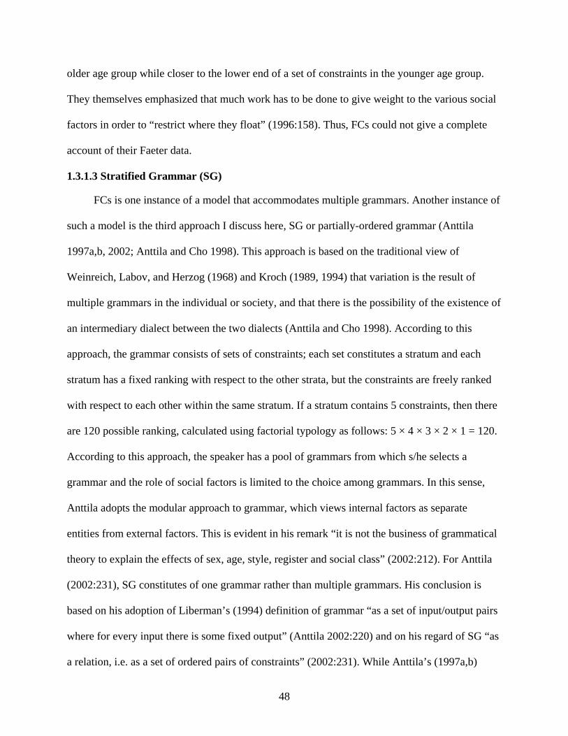
48
older age group while closer to the lower end of a set of constraints in the younger age group.
They themselves emphasized that much work has to be done to give weight to the various social
factors in order to “restrict where they float” (1996:158). Thus, FCs could not give a complete
account of their Faeter data.
1.3.1.3 Stratified Grammar (SG)
FCs is one instance of a model that accommodates multiple grammars. Another instance of
such a model is the third approach I discuss here, SG or partially-ordered grammar (Anttila
1997a,b, 2002; Anttila and Cho 1998). This approach is based on the traditional view of
Weinreich, Labov, and Herzog (1968) and Kroch (1989, 1994) that variation is the result of
multiple grammars in the individual or society, and that there is the possibility of the existence of
an intermediary dialect between the two dialects (Anttila and Cho 1998). According to this
approach, the grammar consists of sets of constraints; each set constitutes a stratum and each
stratum has a fixed ranking with respect to the other strata, but the constraints are freely ranked
with respect to each other within the same stratum. If a stratum contains 5 constraints, then there
are 120 possible ranking, calculated using factorial typology as follows: 5 × 4 × 3 × 2 × 1 = 120.
According to this approach, the speaker has a pool of grammars from which s/he selects a
grammar and the role of social factors is limited to the choice among grammars. In this sense,
Anttila adopts the modular approach to grammar, which views internal factors as separate
entities from external factors. This is evident in his remark “it is not the business of grammatical
theory to explain the effects of sex, age, style, register and social class” (2002:212). For Anttila
(2002:231), SG constitutes of one grammar rather than multiple grammars. His conclusion is
based on his adoption of Liberman’s (1994) definition of grammar “as a set of input/output pairs
where for every input there is some fixed output” (Anttila 2002:220) and on his regard of SG “as
a relation, i.e. as a set of ordered pairs of constraints” (2002:231). While Anttila’s (1997a,b)
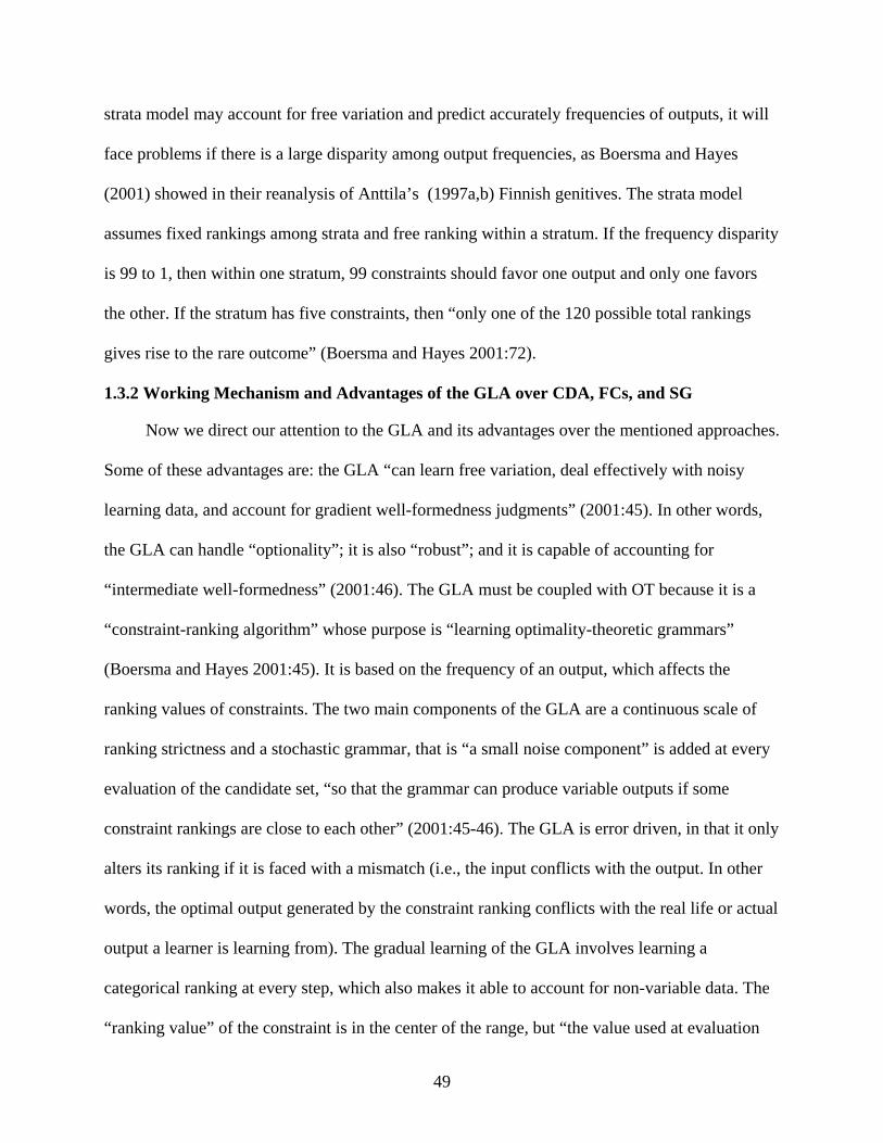
49
strata model may account for free variation and predict accurately frequencies of outputs, it will
face problems if there is a large disparity among output frequencies, as Boersma and Hayes
(2001) showed in their reanalysis of Anttila’s (1997a,b) Finnish genitives. The strata model
assumes fixed rankings among strata and free ranking within a stratum. If the frequency disparity
is 99 to 1, then within one stratum, 99 constraints should favor one output and only one favors
the other. If the stratum has five constraints, then “only one of the 120 possible total rankings
gives rise to the rare outcome” (Boersma and Hayes 2001:72).
1.3.2 Working Mechanism and Advantages of the GLA over CDA, FCs, and SG
Now we direct our attention to the GLA and its advantages over the mentioned approaches.
Some of these advantages are: the GLA “can learn free variation, deal effectively with noisy
learning data, and account for gradient well-formedness judgments” (2001:45). In other words,
the GLA can handle “optionality”; it is also “robust”; and it is capable of accounting for
“intermediate well-formedness” (2001:46). The GLA must be coupled with OT because it is a
“constraint-ranking algorithm” whose purpose is “learning optimality-theoretic grammars”
(Boersma and Hayes 2001:45). It is based on the frequency of an output, which affects the
ranking values of constraints. The two main components of the GLA are a continuous scale of
ranking strictness and a stochastic grammar, that is “a small noise component” is added at every
evaluation of the candidate set, “so that the grammar can produce variable outputs if some
constraint rankings are close to each other” (2001:45-46). The GLA is error driven, in that it only
alters its ranking if it is faced with a mismatch (i.e., the input conflicts with the output. In other
words, the optimal output generated by the constraint ranking conflicts with the real life or actual
output a learner is learning from). The gradual learning of the GLA involves learning a
categorical ranking at every step, which also makes it able to account for non-variable data. The
“ranking value” of the constraint is in the center of the range, but “the value used at evaluation
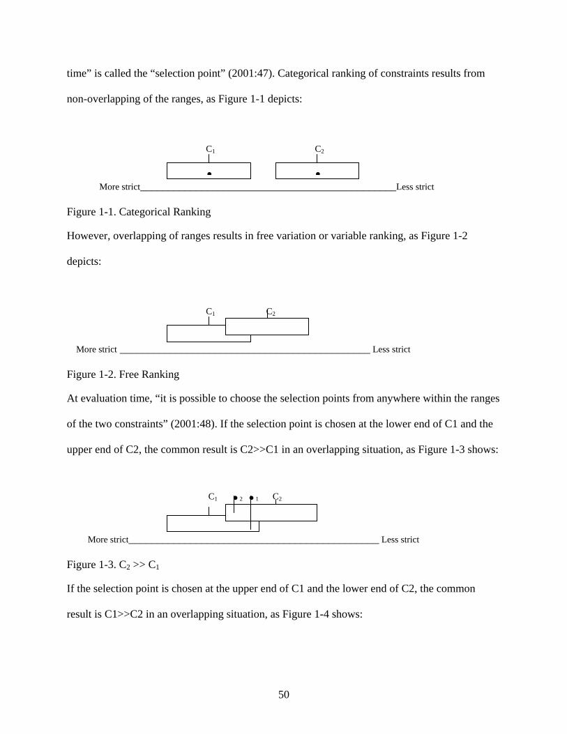
50
time” is called the “selection point” (2001:47). Categorical ranking of constraints results from
non-overlapping of the ranges, as Figure 1-1 depicts:
C1 C2
More strict______________________________________________Less strict
Figure 1-1. Categorical Ranking
However, overlapping of ranges results in free variation or variable ranking, as Figure 1-2
depicts:
C1 C2
More strict _____________________________________________ Less strict
Figure 1-2. Free Ranking
At evaluation time, “it is possible to choose the selection points from anywhere within the ranges
of the two constraints” (2001:48). If the selection point is chosen at the lower end of C1 and the
upper end of C2, the common result is C2>>C1 in an overlapping situation, as Figure 1-3 shows:
C1 .2 .1 C2
More strict_____________________________________________ Less strict
Figure 1-3. C2 >> C1
If the selection point is chosen at the upper end of C1 and the lower end of C2, the common
result is C1>>C2 in an overlapping situation, as Figure 1-4 shows:
• •
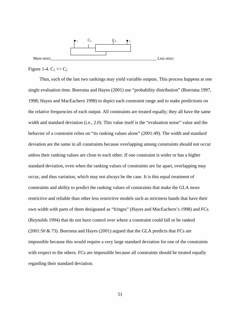
51
.1 C1 C2 .2
More strict_____________________________________________ Less strict
Figure 1-4. C1 >> C2
Thus, each of the last two rankings may yield variable outputs. This process happens at one
single evaluation time. Boersma and Hayes (2001) use “probability distribution” (Boersma 1997,
1998; Hayes and MacEachern 1998) to depict each constraint range and to make predictions on
the relative frequencies of each output. All constraints are treated equally; they all have the same
width and standard deviation (i.e., 2.0). This value itself is the “evaluation noise” value and the
behavior of a constraint relies on “its ranking values alone” (2001:49). The width and standard
deviation are the same in all constraints because overlapping among constraints should not occur
unless their ranking values are close to each other. If one constraint is wider or has a higher
standard deviation, even when the ranking values of constraints are far apart, overlapping may
occur, and thus variation, which may not always be the case. It is this equal treatment of
constraints and ability to predict the ranking values of constraints that make the GLA more
restrictive and reliable than other less restrictive models such as strictness bands that have their
own width with parts of them designated as “fringes” (Hayes and MacEachern’s 1998) and FCs
(Reynolds 1994) that do not have control over where a constraint could fall or be ranked
(2001:50 & 73). Boersma and Hayes (2001) argued that the GLA predicts that FCs are
impossible because this would require a very large standard deviation for one of the constraints
with respect to the others. FCs are impossible because all constraints should be treated equally
regarding their standard deviation.
52
Boersma and Hayes (2001) explained the process of the GLA in 4 steps. In the “initial
state” of the GLA, each constraint is given a value specified by the linguist. The value could be
the same for all constraints or different; the grammar that results after learning nonetheless will
be the same but the amount of input data and computation necessary to learn it differ. The first
step is to present the GLA with a learning datum (i.e., the input) that is the surface form of the
adult, not the learner. The GLA was first used for L1 acquisition. Thus, the child has access only
to the adult surface forms from which s/he learns his/her L1. From those surface forms, the child
learns the L1 grammar and develops an underlying form that mirrors the adult’s surface forms.
However, when using the GLA to model L2 acquisition, in our case a second dialect, the learner
has already developed an underlying form of his L1 in childhood. It is this underlying form that
is used as the input in the GLA and it is this form that undergoes change in the learning process.
This is the core principle of Prince and Smolensky’s (2004 [1993]) idea of Lexicon
Optimization. A learner may or may not be able to restructure his/her underlying form from
exposure to a surface form that does not match his/her underlying form.
The second step is to generate outputs by adding a noise value to the current ranking value
of the constraint to obtain the selection point at every evaluation time. The third step constitutes
comparison. If the generated output matches the learning datum, nothing further is done. If a
mismatch between the learning datum and the generated output occurs, the grammar must be
adjusted; the algorithm takes a learning step and thus alters the grammar. The next step is “mark
cancellation” if the same constraint is violated by both candidates. The fourth step constitutes
“moderate adjustments of the ranking values” (2001:52) to obtain the right result. Since there is
no certainty on whether the constraints with uncancelled marks for the learning datum are too
high or those for the learner’s output are too low, both promotion and demotion take place. The
53
adjustment of the ranking values of constraints involves increasing or decreasing the constraint’s
value by the amount of the plasticity value. Plasticity refers to “the numerical quantity by which
the algorithm adjusts the constraints’ ranking values at any given time” (2001:52). In the “final
state”, the algorithm arrives at the appropriate grammar that generates the adult’s surface form
after cycles of repeating steps 1-4.
Boersma (1998) and Boersma and Hayes (2001) realized the incorrectness of the
predictions of the earlier version of the GLA that was referred to as the Minimal Gradual
Learning Algorithm (MGLA), in which only one constraint, the highest violated constraint by
the intended winner, is demoted and only one constraint, the highest violated constraint by the
intended loser, is promoted. In the GLA, all constraints violated by the correct form are demoted
and all the constraints violated by the incorrect form are promoted. Although Boersma and
Hayes (2001) do not deny that other methods of evaluation, such as the CDA may work well for
non-variable data, they point out that the GLA has many advantages over other models. To test
the GLA and to show that it has advantages over the CDA, they provide empirical evidence by
reanalyzing Hayes and Abad’s (1989) data of metathesis in Ilokano and Hayes and
MacEachern’s (1998) data of English light and dark /l/. What makes the GLA advantageous over
the drastic learning process of the CDA is that it does its job gradually, continuously generating
more correct outputs without causing any damage to the grammar.
To test the GLA against the SG approach to free variation, Boersma and Hayes (2001)
reanalyzed Anttila’s (1997a,b) data of Finnish genitives. They found that SG runs into problems
when faced with large disparity among output frequencies. This makes the GLA more
advantageous than SG. In addition, Antilla thinks that Boersma and Hayes’s (2001) model of
continuous ranking and stochastic constraints may have advantages over other models because of
54
its use of the GLA that enables us to arrive at the right ranking from the surface forms and the
corresponding underlying form. While the multiple grammars model and its derivatives (e.g.,
SG) rely on frequencies and grammar-counting, the continuous ranking approach moves OT in
the direction of quantification.
1.3.2.1 Pure linguistic applications of the GLA
Boersma and Hayes’s (2001) first test of the GLA was Hayes and Abad’s (1989) Ilokano
metathesis data: /w/ optionally becomes [w], where [w] is not an underlying segment, rather
derived from /o/. The process includes: 1) computing “the factorial typology of the constraint set
over the candidates given” and 2) then add gradually “pairwise constraint rankings, recomputing
the factorial typology as constrained a priori by these rankings, until the output set had shrunk to
include only the attested cases of free variation” (2001:61). The CDA could not converge on the
same data, concluding that it cannot account for free variation because, as mentioned above, this
leads to constant demotions of constraints and damaging of the grammar. In contrast, The GLA
was able to converge, did its job gradually without damaging the grammar, and continued to
generate correct outputs.
Another advantage of the GLA is that it can account for intermediate well-formedness
without recourse to different width of ranges or to fringes (Hayes 2000). Hayes and
MacEachern’s (1998) model of strictness bands and fringes is “less restrictive” because “it
permits individual constraints to be affiliated with “bands”, each with its own width, that specify
the range of selection points”. The model also “permits parts of each band to be designated
‘fringes’,” which lead to intermediate well-formedness if a selection point falls within them”
(Boersma and Hayes 2001:73). Being a less powerful theory and being able to account for the
same data, the GLA is advancement to other approaches as it generates its own learning
55
algorithm. To account for intermediate well-formedness, Boersma and Hayes 1) “use one
equation to convert gathered gradient well-formedness judgments into conjectured frequencies;
2) then, they feed these conjectured frequencies into the GLA, “which will produce (if all goes
well) a grammar that closely mimics them” (2001:76) (i.e., predicted frequencies); 3) “by
feeding the predicted frequencies into the mathematical inverse of the first equation”, they get
predicted judgments; and 4) finally, make comparison between the observed judgments and the
predicted judgments. These comparisons show that the grammar learned by the GLA is very
close in form to Hayes’s (2000) fringes.
1.3.2.2 Example of a sociolinguistic application of GLA
After discussing the advantages of the GLA over other models, it would be of interest to
review the only application of it, to the best of my knowledge, to sociolinguistic variation and
change (Cutillas-Espinosa 2004). Like Boersma and Hayes (2001), Cutillas-Espinosa
emphasized two main points: variation is gradual and continuous (2004:171), designating a
special weight to personal choice in variation. His approach involves: (i) a continuous ranking
approach to constraints (Boersma 1997, 2000; Hayes 2000; Boersma and Hayes 2001) and (ii) a
limited number of available grammars, (2004:171) (i.e. his model consists of three grammars to
account for sociolinguistic variation). The first grammar G1 is the standard one that is associated
with prestige, education and propriety. The third grammar G3 is the local grammar that is used by
the community. The second grammar G2 is the default grammar or intermediate grammar that
could be closer to either the first or the third grammar due to various social, personal, or
contextual factors; it is the everyday, informal, and ‘in use’ grammar, characterized as
“dynamic” because it changes according to the speaker’s need (2004:172). Cutillas-Espinosa
suggests that the GLA could account for one of the three grammars that every person has (i.e. the
second/default grammar). In this sense, G2 is assumed to be a continuous ranking of constraints,
56
based on conscious choice of the speaker of the appropriate ranking for the appropriate output in
a particular context. Cutillas-Espinosa assumes that a speaker who is exposed to two different
grammars tends to build his/her own constraint ranking to accommodate the social context, to
build an identity, or to project a self-image. In this sense, grammar is no longer observed as a
mechanism in which personal decisions are not taken into consideration. Rather, a speaker can
control the ranking values of his/her grammar consciously. To quote him “Grammar is no longer
seen as a fully automated mechanism; personal and meaningful decisions are granted a place”
(2004:175).
Cutillas-Espinosa applied the GLA model to both Labov’s (1966) study of the English (r)
that can be realized as [] or Ø in the speech of New York City and to the Castilian Spanish (s) in
Murcia, which can be realized as either [s] or Ø (Hernández-Campoy and Trudgill, 2002). He
examined the case of Susan Salto from Labov’s (1966) study, who showed great stylistic shifts
for the variable (r). She used [] 100% of the time in her most careful style, minimal pairs, and
suppressed it 98% of the time in casual speech. Starting with the fixed ranking value 80 for the
markedness constraint *CODA/r, the results showed that MAX would have the ranking value
91.31 in minimal pairs, ensuring that MAX will be higher ranked than *CODA/r, whereas it will
have the ranking value 68.69 in casual speech, guaranteeing a higher ranking of *CODA/r.
Cutillas-Espinosa also examined the case of a radio presenter at a local station in Murcia (Spain)
from Cutillas-Espinosa and Hernández-Campoy’s (2004) study of the differences in (s) deletion
in the speech of the presenter in two different settings: 1) in broadcasting, talking to non-standard
speaking audience on the phone, whose speech is characterized with suppression of (s), and 2) in
a formal interview with the researchers (Cutillas-Espinosa 2004:176). Cutillas-Espinosa and
Hernández-Campoy (2004) had found that the presenter used the [s], the standard variant, 89% in
57
broadcasting and only 1% in the interview. Cutillas-Espinosa conducted the same analysis done
on the previous study and found that the ranking value of MAX correlated with the style chosen
by the presenter: 83.46 in broadcasting and 73.4 in interview. Thus, he assumed fixed ranking for
markedness constraints and that faithfulness constraints are the ones that change ranking value
and move around to arrive at the desired output. For him, the continuous ranking scale overrides
all other models (FCs, CDA, and SG), in that it can feature a continuum of grammar where style
can shift gradually, rather than abruptly. His approach is more of the antimodular type because it
takes both internal and external factors into consideration in opposition to Anttila’s (1997a,b,
2002) modular approach that only takes internal factors into consideration.
Cutillas-Espinosa’s model is insightful and it opens a field of sociolinguistic investigation
within an Optimality-Theoretic approach, embellished with the numerical and functional
workings of the GLA. In this study, I will elaborate on this insightful model by taking into
account that the human mind may not be limited to three particular grammars and the observed
intra-speaker oscillation and inter-speaker differences in adopting or acquiring a new grammar. I
also introduce social factors as constraints to the GLA and interweave them with linguistic
constraints to show their immediate effect on the ranking values of linguistic constraints and the
choice of one grammar over another at a certain time and place. One further advancement is
showing which social constraints are activated or not, and to what extent, by certain speakers or
groups of speakers at a certain time and place. In addition, I would like to stress the differences
that may be observed among individual grammars within the same community or the same group
of speakers. In this study, I am also using my own original data that is based on naturally
occurring speech to see if all speakers behave in the same way regarding choices made among
grammars, and if the pattern is uniform throughout the community. A larger sample of speakers
58
and a comparison among the different grammars used by the speakers may give us a better
understanding of these differences. Furthermore, G1 and G3 may not be stable as well; they may
be variable and might be presented on a continuous ranking scale. In Arabic, for example, the
standard language itself is variable: not all speakers use the same level of Case marking or their
degree of reverting to the vernacular may vary within the same formal setting.
1.3.2.3 Concluding remarks about the GLA
The discussion above reveals many advantages of the GLA over other models. The last
example shows the possibility of applying it to sociolinguistic variation and change and naturally
occurring speech. It remains to be seen if one can include social factors in the computational
process of the GLA as ranked constraints. In addition, the non-teleological approach (Boersma
1997b) to the GLA may need some revision, in my opinion, because if selection and choice play
a role in determining the ranking value of constraints, then there might be some teleological
effects in the adults’ acquisition of a second grammar. The non-teleological approach to the GLA
might work well in its application to L1 acquisition, not to dialectal and sociolinguistic variation
where social factors can be involved and play a selective role. Thus, social factors may influence
the ranking values and rankings of linguistic constraints. In applying the GLA to sociolinguistic
variation, one can predict the ranking values of constraints and depict the intrapersonal and
interpersonal oscillation that one may observe in the speech of those who try to change the way
they speak in attempt to sound city-like, more prestigious, or probably more or less formal. The
stochastic feature of constraints and the continuous feature of ranking should be applicable to
social factors because sociolinguistic variation is gradual and stochastic in nature. Not all
speakers behave in the same way or have the same level of sociolinguistic competence. Even the
same speaker may vary his/her speech along a continuous scale of values. Sometimes, there is a
kind of internal conflict between grammars, leading to confusion regarding the choice of one
59
grammar over another or a kind of stalemate situation where the speaker/learner is in an
intermediate position from which s/he cannot escape.
In the same way that social factors should be included in formal theory, sociolinguistics
should take markedness into account, because markedness, in addition to social factors, does
sometimes play a major role in language variation and change (Reynolds 1994). This markedness
could have played a major role historically in producing the SA [] and [] as [t] as [d]
respectively. The merger of [] and [] with [t] and [d] respectively was completed around the
14th century (Daher, 1998a, 1999). This is comparable to the use of Thai, Russian, German, and
Japanese learners of English of [t] and [s] instead of [] because of the absence of this sound
from their inventory, which is attributed to the interaction of faithfulness and markedness
constraints (Lombardi 2003).
1.4 Conclusion
A number of studies have employed OT in one way or another to account for language
variation from various perspectives. While most researchers agree that sound systems change
continuously (Boersma 1997b; Labov 1994; Ohala 1993), even if the change only results from
“internal factors” (Boersma 1997b: 1), they may disagree on the reason behind sound change.
Sound change does not have to be teleological (Boersma 1997b; Ohala 1993), facilitative or
based on meaning preservation (Labov 1994). It could be based on historical factors (Adam
2002) or perceptual and lexicon optimization reasons (Holts 1997). However, Boersma (2000)
argues that optimization is not the main “internal factor” (Boersma 2000: 1) for sound change.
Thus, most of the language variation studies that implement OT do not deal with sociolinguistic
variation and do not refer to the social interface with the linguistic and historical factors that
commonly involve internal, perceptual, or lexicon optimization factors. Unlike other studies, this

60
study deals with variation from a social perspective where social factors play a major role in the
change. They are integrated into the mental computing system of the speaker in the form of
constraints that intersect with linguistic constraints to account for real life occurrences of
particular variants. The study reflects the intra- and inter-speaker preference for certain sounds
according to the interlocutor, although the speaker is capable of pronouncing both sounds of both
dialects perfectly. The situation is similar to knowing two languages and switching between the
two according to the interlocutor. The difference is that the switch is not done for the sake of
comprehension on the part of the interlocutor but for the sake of competing with the interlocutor
for prestige. This is the case that we will observe concerning the two variants [q] and [].
It would thus be of interest to see how one can model this sociolinguistic variation within
the framework of OT and the GLA and how one can incorporate social constraints into the
human mind computing system. This may give us an answer to how speakers oscillate between
two different dialects and how the degree of social success that those speakers achieve depends
on the level of acquisition of the new dialect. It may also explain the intra- and inter-speaker
variation observed among speakers who use more than one variety, in an attempt to
accommodate the speech of the interlocutor. Thus, at the core of this study is the development of
a model for variation and change that could have cross-linguistic implementations. The model
will present how the intersection of linguistic constraints with social constraints can model and
predict real life variable use of variants as well as predict the direction of change when
constraints are given specific values. This model will also highlight the importance of social
constraints in determining the ranking values of other constraints as well as the chosen grammar
at a certain time and place. The model will show that variation within the speech of a community
could be driven by various factors at the same time. While one variation may be led by social

61
factors, another variation could have been led by markedness diachronically and be maintained
by faithfulness constraints synchronically. I will also show that this model can account for these
different types of variation within the same dialect. It can deal with these different variations
independently from each other since these variations are the result of different factors and act
independently from each other. This discussion provokes a number of research questions that
will be stated in Section 1.5.
1.5 Research Questions
The research questions that guide this study are:
1. How can Optimality Theory account for speakers’ switches between two different dialects
and their intrapersonal and interpersonal variation in the use of particular sounds (e.g., the
use of [] in place of [q]) based on their interlocutor’s background?
2. How can social factors be incorporated into the GLA?
3. To what degree do social factors play a role in building our grammars, or rather developing
new grammars?
4. How consistent is the pattern of variation and sound change within and among rural
migrant speakers to the city of Hims?
5. Which factors are stronger in leading a sound change: markedness constraints or social
constraints?
1.6 Structure of the Study
The study is organized as follows. Chapter 2 presents the methodology used in data
collection and analysis. It includes a brief description of the community under investigation. It
introduces the city of Hims, the speech sample, the linguistic and social variables, and a brief
62
description of data analysis, including the statistical models and other quantitative methods
employed.
Chapter 3 introduces the theoretical analysis of the study. In this chapter, the new model
proposed in this study will be explored in detail. The chapter begins with descriptions of the
Himsi and rural grammars and the change that the rural migrant speaker grammar undergoes in
his/her attempt to appear prestigious. Then, social constraints and the stochastic process that is
followed in examining the simultaneous effect of social and linguistic constraints on the choice
of a grammar at a certain time and place are introduced. This chapter shows that social
constraints should constitute an essential part of our grammar. The inclusion of social constraints
in OT and the GLA yields results that match real life occurrences. These social constraints play a
major role in determining the grammar chosen by certain speakers from a certain age group,
gender, residential area, and social class, particularly in the use of socially conditioned variants,
such as [q] and []. Including social constraints in the computation explains the variability in the
use of [q] and [] among speakers from the same social group or different social groups. Chapter
3 also shows that certain social constraints give us expectations on what the speech of a certain
speaker or a group of speakers should sound like. The same model deals with other types of
phenomena independently from the sociolinguistic variation between [q] and []. It shows that
social constraints do not play a role in the stable use of [t] and [s] and [d] and [z]. The chapter
shows that each of these four sounds has an underlying form that is identical to its surface form.
Faithfulness constraints play a major role in maintaining the input in the output.
Chapter 4 presents the quantitative analysis regarding the use of the two sociolinguistic
variants [q] and []. In this chapter, I explore the association between social class and education,
income, occupation, and residential area. Income, occupation, and residential area emerge as
63
significant indicators of social class, whereas education emerges as insignificant. These findings
correspond with my predictions of how social class should be determined in Syria and other
Arab countries. I show that there is correlation between the two variants [q] and [], using a Chi-
squared Bivariate test. I also explore the distribution of the data with respect to each of the
independent variables to determine the type of statistical tests that should be implemented. The
non-normality of the distribution and the overdispersion of the data called for the use of Negative
Binominal regression procedures. In the main effects tests on both [q] and [], age, gender, and
residential area emerged as significant factors in determining the use of [q] and []. However, in
the interaction tests, residential area emerged as insignificant regarding the use of []. This result
added one advantage to the model proposed in Chapter 3. Making social factors more specific by
dividing them into a number of social constraints and implementing them in the GLA enables us
to see interaction between one of the constraints of a social factor and other constraints. This
specificity shows that the whole social factor does not have to be involved in the variation, but
part of it may. Chapter 4 further examines whether frequency plays a role in acquiring certain
words before other words. Frequency emerges as a facilitative factor in the acquisition of the
prestigious form. Highly frequent words appear with [] in the speech of varying speakers more
than less frequent words.
Chapter 5 presents a quantitative analysis of the use of [t] and [s] and [d] and [z]. Because
this stable phenomenon is not socially conditioned, frequency effects are explored against two
diachronic changes that led to the replacement of the SA [θ] and [] with [t] and [d] first and
later with [s] and [z] respectively. Today, the use of the four variants is stable due to two
opposing frequency effects (Bybee 2001). The first frequency effect led to the first diachronic

64
change and the merger with [t] and [d]. The second frequency effect made highly frequent words
resistant to the new creeping change: the use of [s] and [z] in place of [θ] and [] in borrowed
words from SA. That is why we observe the use of [t] and [d] in highly frequent words in
comparison to the use of [s] and [z] in less frequent words.
Chapter 6 concludes this work. It gives a brief answer to each of the five research
questions that led this research. It also highlights other findings of the study such as the role
frequency plays in both the use of [q] and [] and [t] and [d] and [s] and [z]. It also lists the
advantages of and caveats about the new model. It gives suggestions and recommendations for
future research, showing the possibilities of expanding on the social constraints proposed in this
study. In general, the conclusion calls for exploring the possibility that social constraints could
be universal in the same way that linguistic constraints are.
65
CHAPTER 2 METHODOLOGY
2.1 Setting: The City of Hims
The city we are concerned with in this study is Hims or Homs, as some people refer to it as
a result of rounding the first vowel that is also a feature of the Himsi dialect. Hims is the third
most important city in Syria and it is strategically located in the fertile Orontes River Valley in
the central western part of Syria (Figure 2-1) on a hill approximately 450 meters above sea level.
It is a crossroad between the capital Damascus 160 km to the south and the second major city
Aleppo 190 km to the north and between coastal cities to the west, such as Tartus and Latakia
and the eastern cities of Syria, such as Palmyra (in Arabic Tadmur) and Dayr az Zawr. Hims,
known in Roman times as Emesa, is an ancient city dating back to the year 2300 B.C. (The
Colombia Encyclopaedia 2007). The population of the City of Hims, according to 2002 estimates
provided by the Homs City Council (2008), is 1,033,000. The city of Hims is the capital of the
Hims Governorate, which is the largest among other Syrian governorates (40,940 square
kilometer) (Syrian Arab Republic Central Bureau of Statistics 2002). The population of the Hims
Governorate according to civil registration records is 1,791,000 (Arab Republic Central Bureau
of Statistics 2004). This number includes both urban and rural areas (i.e., the city of Hims and
the surrounding villages respectively). Excluding those who live outside Syria, the number of
physically present residents of the Hims Governorate is estimated at 1,577,000.
The important strategic location and size of the Hims Governorate distinguish it from other
Syrian governorates. It is the third governorate in industry, trade, and agriculture. The city itself
is the “third largest industrial city in Syria” (Gilford 1978). The centrality of the city of Hims
makes it an attractive center to a large number of rural people from the neighboring countryside.
Those rural migrants find haven in Hims’ Al-Baath University, the third major public university
66
in Syria, job market, and shopping and trading centers. From the late sixties and early seventies,
a larger influx of rural migrants to major cities in Syria, particularly Hims, started taking place.
Rural people started abandoning agriculture and their lands in their villages. With the
government facilitating education and making it available free to everyone, they sought higher
education to obtain governmental jobs, such as teaching, construction, and industry that includes
the refinery and other major phosphate and chemical plants all of which are situated in Hims.
However, Zakaria and Sibai (1989 cited in Mahayni 1990) suggest that migration was not only a
response to industrialization but also to the dire socioeconomic situation in many rural areas of
Syria. Thus, they suggest that the search for better life style and higher level of income motivates
many to move to the city, particularly those with higher levels of education. In addition to the
growth of sectors such as building and construction and social and personal services, the higher
growth in the government sector provided more employment opportunities for the educated from
the rural areas, inducing more migration (Mahayni 1990). Mahayni (1990) traced the population
growth of both urban and rural areas in the Syrian governorates between the years 1960 and 1986
based on statistics from the Syrian Arab Republic Central Bureau of Statistics (1960, 1986). He
found that the population of the city of Hims increased annually by 4.76% from 150,000 in 1960
to 502,000 in 1986, whereas the annual population growth of rural areas increased by 2.43%
from 251,000 in 1960 to 469,000 in 1986. The higher growth rate of the population of the city of
Hims is not ascribed to higher birth rate in the city; rather, it is the result of the migration of huge
numbers of rural dwellers to the city of Hims. The proportion of rural migrants who lived in the
city of Hims in 1970 was 25.4% of the total city population according to the Syrian Arab
Republic Central Bureau of Statistics (reported in UNCEWA 1980).
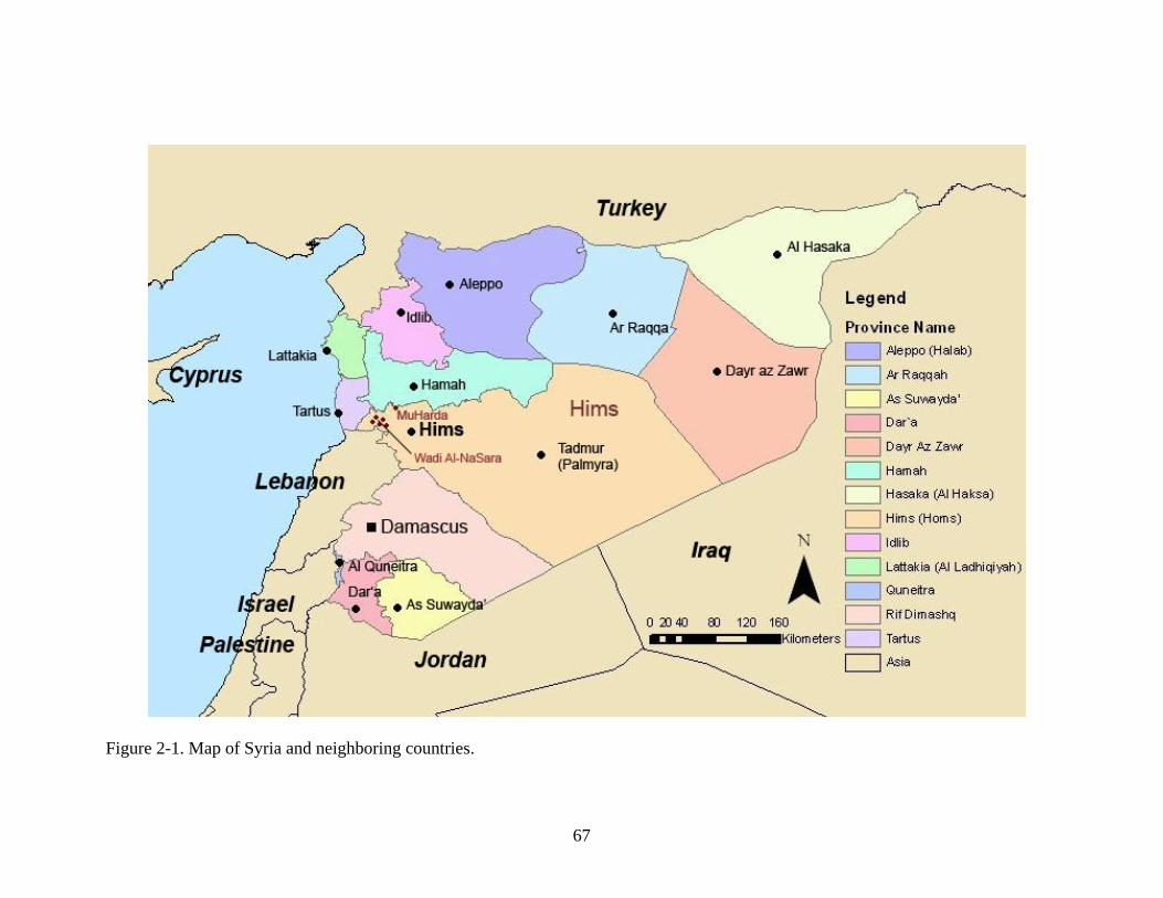
67
Figure 2-1. Map of Syria and neighboring countries.
68
Rural migration to big urban centers, such as Hims, is not only a Syrian phenomenon but
also a phenomenon of many Arab countries that were developing and growing industrially. For
example, Casablanca in Morocco has seen a huge influx of rural migration in the second half of
the twentieth century because of industrialization (Hachimi 2005, 2007). This migration also
resulted in “social, cultural and linguistic changes” (Hachimi 2007: 97). Thus, rural migration to
urban (e.g., Hims) or urbanized (e.g., Casablanca) centers seems to be a wide spread
phenomenon in the Arab world and usually results in linguistic variation because of language
contact among various language varieties.
Hims, like other Syrian cities, is home to a diverse population of Sunnis, Alawites, and
Christians as well as Armenians and Palestinian refugees. Before the Arab conquests after the
birth of Islam in 622 A.D., Hims was mainly populated by Christians. It was taken by Muslims
in 636 A.D. and the large Christian element of the city was eliminated after the rebellion in 855
A.D. (Encyclopedia Britannica 2008). However, Hims continues to have smaller concentrations
of Christians in different residential areas and contains historically significant ancient churches
from early Christianity, such as Umm Al-Zunnar (The Virgin Mary’s Girdle) and Mar Elian (St.
Elias). These churches are situated in Al-Hameeddieh, one of the residential areas from which
most of the participants (39 speakers) in this study come. Hims is also surrounded by a collection
of Christian villages called Wadi Al-Nasara ‘The Valley of the Christians’ from which almost all
of the study participants come (Section 2.1.2).
The Himsi people are known for their pride in their dialect, which is characterized by the
use of []. For this reason, they usually stigmatize other dialects, particularly the ones that
contain the [q] sound such as many nearby rural dialects. The stigmatization of the use of [q]
leads the rural people to adopt the [] and other speech features of the city people, so they can
69
integrate into and be accepted as part of the urban community. The use of [] instead of [q] is
considered more urbane in major Syrian cities, such as Damascus (Daher 1998a, 1998b) and
Aleppo. Thus, many rural migrants start switching to the use of [] instead of [q] and
consequently switch to other speech features.
2.2 Speech Sample
Thus, the center of investigation is the speech community of the city of Hims to which
many rural speakers have migrated at one point in their life. The study greatly depends on
naturally occurring speech from speakers who are not picked at random. According to Labov
(1966: 43), the effects of the “observer’s paradox” may be partially overcome by obtaining
samples from natural social interactions among in-group members (e.g., interacting with family
members or “peer group”). The speech sample is taken from rural migrant speakers who belong
to the Christian community at large to which I myself belong. They reside in two residential
areas in Hims: Al-Hameeddieh and Akrama (Section 2.3.2 and Figure 2-2).
One important criterion when choosing the participants was being rural migrants to the city
of Hims, representing the first generation, or the sons and daughters of those migrants who were
born in the city of Hims, representing the second generation. In this sense, the study focuses on
two generations or age groups: older and younger. Both male and female speakers were chosen
from different economic and social background. With the exception of Speakers 19 & 5, all other
participants come from the collection of the Christian villages called Wadi Al-Nasara (Figure 2-
1) and mainly from the village of Oyoun Al-Wadi (thereafter Oyoun) ‘The Springs of the
Valley’. The reason for choosing the village Oyoun and other neighboring villages is that I am
originally from that village and familiar with the surrounding villages. Being an in-group
member adds more naturalness to the conversations, having the opportunity to interview people
70
who are relatives, friends, family members, and neighbors. Being an in-group member has been
emphasized by many researchers as the most preferable method to obtain the most naturalistic
speech data (e.g., Labov 1972a; Eckert 1991; Milroy & Milroy 1992). Hence, integrating into the
investigated speech community has been the focus of many ethnographic studies, which required
researchers to spend a long period getting to know the community (e.g., Gal 1978; Eckert 1989;
Milroy 1980). Fortunately, I have had the advantage of being part of the community under
investigation in this study. My own family is from the village of Oyoun, and I moved to Hims at
the age of two years and two months. Most of the speakers moved to the city around the same
time like my parents in the mid seventies, and we have strong social ties with them in one way or
another. At home, my family uses the village dialect, but with distant friends and acquaintances,
there is a switch to the Himsi dialect. Thus, I am acquainted with both dialects. This
phenomenon of switching between two forms or two dialects is apparent in the speech of many
rural migrants who live in the city and occasionally go back to visit the countryside.
A sample of fifty-two interviews comprises the data set (Table 2-1). The data were
collected on two separate field trips to Syria. One trip took place in 2004; the other one was in
2006. In my first trip to Syria, I recorded forty-two speakers of whom I only investigate twenty-
six speakers, those who fall within the age ranges that I am investigating in this study. During
my second trip to Syria, I recorded thirty-six participants of whom I only investigate twenty-six
speakers. Ten of the twenty-six speakers, who were recorded in 2004, were rerecorded in 2006
with the purpose of obtaining better sound quality as I was using a more advanced digital
recorder with better voice reception equipment. Their recordings from 2006 are used in this
study. The other sixteen speakers constitute new participants. In my first trip to Syria, I was able
to record more participants because I went in a time of the year – May and June – when it was
71
easy to find participants and record them; people had not yet started their summer vacations.
Most of the people were still in the city because schools and universities were still open;
university and school exams usually finish by the end of June. On my second trip, it was more
difficult to get in touch with participants because July and August are the main vacation months
for people in Syria. Most people commute a great deal more in these two months between the
city and the village as well as take trips to the beach and other excursion trips. The fifty-two
speakers are almost equally distributed between males (24) and females (28); lower middle class
(29) and upper middle class (23); and younger age group (18-35) (24) and older age group (52+)
(28). It is important to have a varied sample to examine the variable use of [q] and []; [], [d],
and [z]; and [], [t], and [s]. Most of the participants – fourty participants – come from the
village of Oyoun where [q] is dominant. The other twelve participants come from the
neighboring Christian villages, Wadi Al-Nasara, in which [q] is dominant. In addition, those
twelve participants are either married to someone from Oyoun or are the son or daughter of one
parent from Oyoun, and his/her other parent is from a neighboring village that has the same
speech characteristics of Oyoun. For example, Speaker-1 is from Tin Sbil and married to
Speaker-14 from Oyoun; Speaker-8 is from Juwaikhat and married to Speaker-20 from Oyoun;
Speakers 33, 34, & 43 are the two sons and daughter of Speakers 8 & 20; Speakers 9 & 26 are
from Ain Al-Ajooz and are husband and wife; Speaker-17 is from Habb Nimra; Speaker-21 is
from Treez and married to Speaker-6 from Oyoun; and Speaker-42 is the daughter of a man from
Oyoun. Speaker-19 is from Muharda; Speaker-5 is from Ilbi and married to Speaker-22 from
Oyoun. Muharda and Ilbi are not in Wadi Al-Nasara, but they are also Christian villages
characterized by the use of [q].
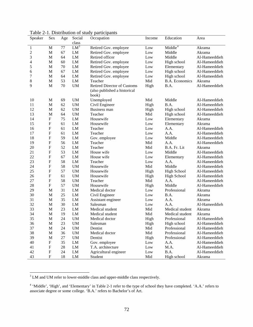
72
Table 2-1. Distribution of study participants Speaker Sex Age Social
class Occupation Income Education Area
1 M 77 LM3 Retired Gov. employee Low Middle4 Akrama 2 M 67 LM Retired Gov. employee Low Middle Akrama 3 M 64 LM Retired officer Low Middle Al-Hameeddieh 4 M 60 LM Retired Gov. employee Low High school Al-Hameeddieh 5 M 70 LM Retired Gov. employee Low Elementary Al-Hameeddieh 6 M 67 LM Retired Gov. employee Low High school Al-Hameeddieh 7 M 64 LM Retired Gov. employee Low High school Al-Hameeddieh 8 M 53 LM Teacher Mid B.A. Economics Akrama 9 M 70 UM Retired Director of Customs
(also published a historical book)
High B.A. Al-Hameeddieh
10 M 69 UM Unemployed Mid Middle Al-Hameeddieh 11 M 62 UM Civil Engineer High B.A. Al-Hameeddieh 12 M 62 UM Business man High High school Al-Hameeddieh 13 M 64 UM Teacher Mid High school Al-Hameeddieh 14 F 75 LM Housewife Low Elementary Akrama 15 F 61 LM Housewife Low Elementary Akrama 16 F 61 LM Teacher Low A.A. Al-Hameeddieh 17 F 61 LM Teacher Low A.A. Al-Hameeddieh 18 F 59 LM Gov. employee Low Middle Al-Hameeddieh 19 F 56 LM Teacher Mid A.A. Al-Hameeddieh 20 F 52 LM Teacher Mid B.A. Fr. Lit Akrama 21 F 53 LM House wife Low Middle Al-Hameeddieh 22 F 67 LM House wife Low Elementary Al-Hameeddieh 23 F 58 LM Teacher Low A.A. Al-Hameeddieh 24 F 58 UM Housewife Mid Middle Al-Hameeddieh 25 F 57 UM Housewife High High School Al-Hameeddieh 26 F 61 UM Housewife High High School Al-Hameeddieh 27 F 58 UM Teacher Mid A.A. Al-Hameeddieh 28 F 57 UM Housewife High Middle Al-Hameeddieh 29 M 31 LM Medical doctor Low Professional Akrama 30 M 25 LM Civil Engineer Low B.A. Akrama 31 M 35 LM Assistant engineer Low A.A. Akrama 32 M 30 LM Salesman Low A.A. Al-Hameeddieh 33 M 23 LM Medical student Mid Medical student Akrama 34 M 19 LM Medical student Mid Medical student Akrama 35 M 24 UM Medical doctor High Professional Al-Hameeddieh 36 M 23 UM Salesman High High school Al-Hameeddieh 37 M 24 UM Dentist Mid Professional Al-Hameeddieh 38 M 36 UM Medical doctor Mid Professional Al-Hameeddieh 39 M 27 UM Dentist High Professional Al-Hameeddieh 40 F 35 LM Gov. employee Low A.A. Al-Hameeddieh 41 F 28 LM T.A. architecture Low M.A. Al-Hameeddieh 42 F 24 LM Agricultural engineer Low B.A. Al-Hameeddieh 43 F 18 LM Student Mid High school Akrama
3 LM and UM refer to lower-middle class and upper-middle class respectively.
4 ‘Middle’, ‘High’, and ‘Elementary’ in Table 2-1 refer to the type of school they have completed. ‘A.A.’ refers to associate degree or some college. ‘B.A.’ refers to Bachelor’s of Art.
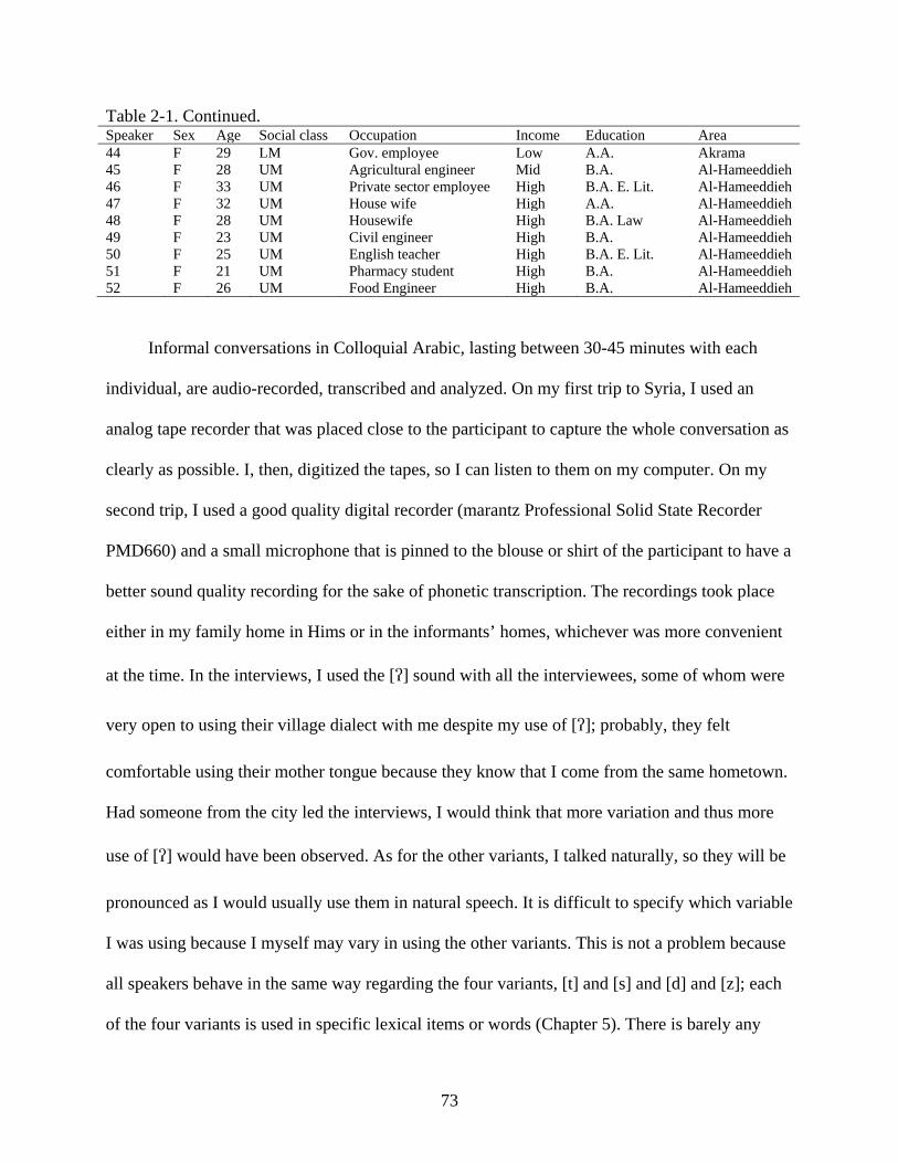
73
Table 2-1. Continued. Speaker Sex Age Social class Occupation Income Education Area 44 F 29 LM Gov. employee Low A.A. Akrama 45 F 28 UM Agricultural engineer Mid B.A. Al-Hameeddieh 46 F 33 UM Private sector employee High B.A. E. Lit. Al-Hameeddieh 47 F 32 UM House wife High A.A. Al-Hameeddieh 48 F 28 UM Housewife High B.A. Law Al-Hameeddieh 49 F 23 UM Civil engineer High B.A. Al-Hameeddieh 50 F 25 UM English teacher High B.A. E. Lit. Al-Hameeddieh 51 F 21 UM Pharmacy student High B.A. Al-Hameeddieh 52 F 26 UM Food Engineer High B.A. Al-Hameeddieh
Informal conversations in Colloquial Arabic, lasting between 30-45 minutes with each
individual, are audio-recorded, transcribed and analyzed. On my first trip to Syria, I used an
analog tape recorder that was placed close to the participant to capture the whole conversation as
clearly as possible. I, then, digitized the tapes, so I can listen to them on my computer. On my
second trip, I used a good quality digital recorder (marantz Professional Solid State Recorder
PMD660) and a small microphone that is pinned to the blouse or shirt of the participant to have a
better sound quality recording for the sake of phonetic transcription. The recordings took place
either in my family home in Hims or in the informants’ homes, whichever was more convenient
at the time. In the interviews, I used the [] sound with all the interviewees, some of whom were
very open to using their village dialect with me despite my use of []; probably, they felt
comfortable using their mother tongue because they know that I come from the same hometown.
Had someone from the city led the interviews, I would think that more variation and thus more
use of [] would have been observed. As for the other variants, I talked naturally, so they will be
pronounced as I would usually use them in natural speech. It is difficult to specify which variable
I was using because I myself may vary in using the other variants. This is not a problem because
all speakers behave in the same way regarding the four variants, [t] and [s] and [d] and [z]; each
of the four variants is used in specific lexical items or words (Chapter 5). There is barely any
74
doubt or rather it is predictable which variant will occur in a certain word. No one was informed
of the exact focus of the study. When they asked about the purpose of the study, they were
informed that it deals with the social influence on sound change, but no specific details were
added. However, the participants were instructed that the interviews were intended to be as
natural and as informal as possible, so they should not put any effort into thinking about what
they should or should not say. In addition, they were informed that their identity as well as their
conversation would be highly confidential. All of the conversations were natural and did not
follow any preconceived format. Topics of the conversations varied, allowing the speaker to talk
about any subject that appealed to him/her (e.g., telling jokes; funny, sad, or frightening stories;
relating dreams; work, love, marriage, and relationships stories; family issues; and other personal
interests). Thus, the interviewees were free to speak about any topic they wanted. Conversations
mostly started by my asking the participant about his/her family, children and other matters of
mutual interest. After some questions and answers, if the conversation slowed down or there was
not much to say, informants were asked to tell a happy or sad story, a dream, or an experience
that they had experienced. To maintain the naturalness of the conversation, other family
members were allowed to be present during the recording of all the participants. Thus, occasional
intervention from other attendees sometimes heated the conversation and made the speaker more
oblivious of the tape recorder.
It is worth noting that some of the speakers are related to each other. Speakers 35, 36, 46,
47, & 48 are respectively the two sons and three daughters of Speakers 12 & 28. Speaker-52 is
the daughter of Speaker-25. Speakers 49, 50, & 51 are sisters. Speakers 45, 37, & 38 are
respectively the daughter and two sons of Speakers 27 & 13. Speakers 44, 29, 30 & 31 are
respectively the daughter and three sons of Speakers 15 & 2. Speakers 33, 34 & 43 are
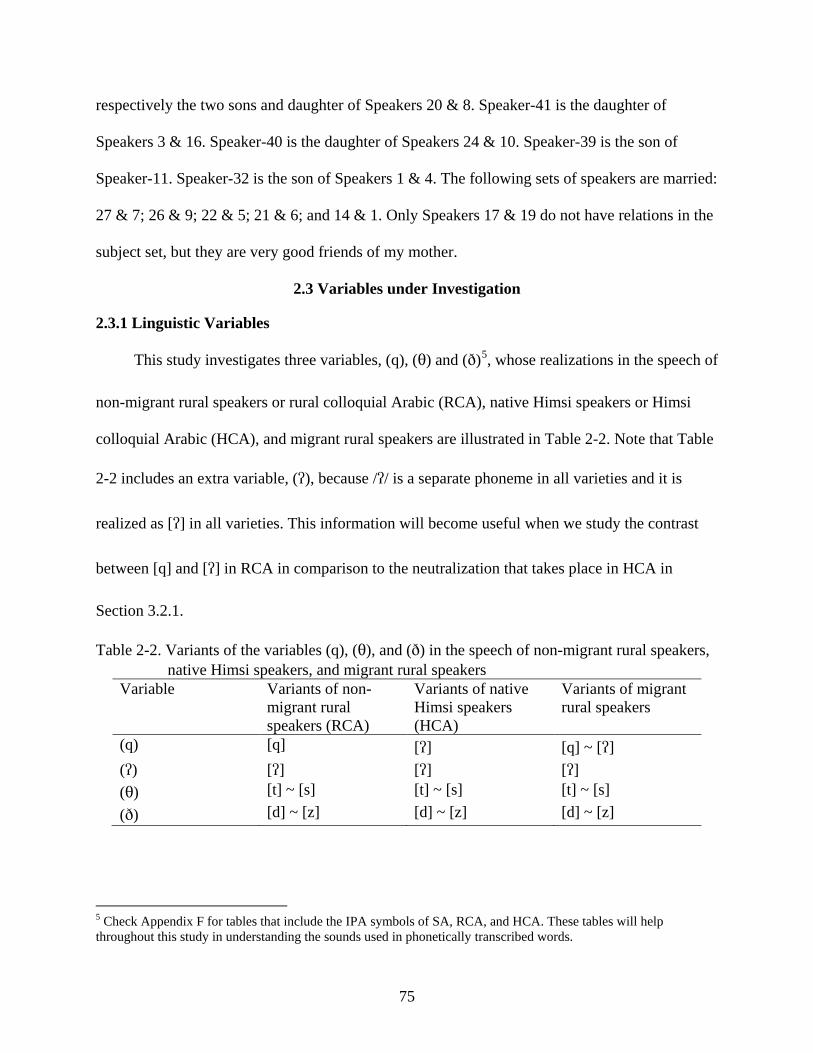
75
respectively the two sons and daughter of Speakers 20 & 8. Speaker-41 is the daughter of
Speakers 3 & 16. Speaker-40 is the daughter of Speakers 24 & 10. Speaker-39 is the son of
Speaker-11. Speaker-32 is the son of Speakers 1 & 4. The following sets of speakers are married:
27 & 7; 26 & 9; 22 & 5; 21 & 6; and 14 & 1. Only Speakers 17 & 19 do not have relations in the
subject set, but they are very good friends of my mother.
2.3 Variables under Investigation
2.3.1 Linguistic Variables
This study investigates three variables, (q), () and ()5, whose realizations in the speech of
non-migrant rural speakers or rural colloquial Arabic (RCA), native Himsi speakers or Himsi
colloquial Arabic (HCA), and migrant rural speakers are illustrated in Table 2-2. Note that Table
2-2 includes an extra variable, (), because // is a separate phoneme in all varieties and it is
realized as [] in all varieties. This information will become useful when we study the contrast
between [q] and [] in RCA in comparison to the neutralization that takes place in HCA in
Section 3.2.1.
Table 2-2. Variants of the variables (q), (), and () in the speech of non-migrant rural speakers, native Himsi speakers, and migrant rural speakers
Variable Variants of non-migrant rural speakers (RCA)
Variants of native Himsi speakers (HCA)
Variants of migrant rural speakers
(q) [q] [] [q] ~ [] () [] [] [] () [t] ~ [s] [t] ~ [s] [t] ~ [s] () [d] ~ [z] [d] ~ [z] [d] ~ [z]
5 Check Appendix F for tables that include the IPA symbols of SA, RCA, and HCA. These tables will help throughout this study in understanding the sounds used in phonetically transcribed words.
76
2.3.1.1 The variable (q)
One of the dependent variables of the study is (q), which is realized in the speech of the
Himsi community, including native Himsi speakers and rural migrants, as two variants: [q] and
[] (Table 2.2). Native Himsi speakers always use [], whereas rural migrants may vary between
[q] and [], taking into account that [q] is their native form. There is no specific phonological
context in which [] occurs as a replacement for [q] in the speech of rural migrants. It can occur
in many phonological contexts except in certain lexical borrowings from SA, such as [quraan]
‘Qur’an’, [liqaa] ‘meeting’, and [aqaafe] ‘cultural’. For example, the rural migrants’ words
[qalem] ‘pen’, [raqbi] ‘neck’, and [wareq] ‘paper’ become [alam], [rabi], and [wara]
respectively in the speech of those who adopt the Himsi variant []. These examples show that
the change could occur word-initially, word-internally, and word-finally. One can also observe in
the given examples that the change from [q] to [] could also be accompanied by vowel changes,
such as the change of [e]6 to [a] in [qalem] and [alam] and [wareq] and [wara]. This is not the
case with all speakers. The change from [q] to [] could act independently from vowel changes.
However, this is beyond the scope of this study.
6 This is what is called an imala. This feature exists in some Arabic dialects; it is defined as the use of [e] instead of [a] or [ee] instead of [aa]. imala is a feature of the rural dialects under investigation, and it usually undergoes change in the speech of rural migrant speakers who accommodate the Himsi forms, [a] and [aa], to appear prestigious. imala exists in some central Syrian dialects (Versteegh 1997:153), which include the rural dialects under investigation. It is a historical change from a > e in different linguistic environments. In Northern Syrian dialects, such as the dialect of Aleppo, this change takes place in the neighborhood of an [i] vowel or when the [a] vowel occurs after consonants (e.g., lisan > lsen ‘tongue’, ami > eme ‘mosque’, kateb > keteb ‘writing’, and taleb > teleb ‘striving’) (Versteegh 1997). The change in the speech of migrant rural speakers takes the opposite direction of that historical change, i.e. [e] becomes [a], in order to sound urbane. Nonetheless, this vowel change is beyond the scope of this study and requires further investigation.
77
It is worth noting that lexical borrowings are excluded from this study because rural and
urban people pronounce them the same. Including them may skew the results, particularly in the
speech of professionals who use a number of jargon words from their own profession and repeat
them many times in their speech. Hence, excluding lexical borrowings from the data yields better
results and gives a better picture of the variation among the various groups of speakers. Ferguson
(1997) and Daher (1998a, 1998b) emphasize that the use of [q] in some words in Damascene
Arabic, which is characterized by the use of the glottal stop as a replacement to the /q/ sound in
Classical/Standard Arabic, is the result of lexical borrowing. Haeri (1991, 1996) also attributes
the existence of [q] in some words in Cairene Arabic to lexical borrowing. In a study (2005) of
‘The role of social factors, lexical borrowing and speech accommodation in the variation of [q]
and [] in the colloquial Arabic of rural migrant families in Hims, Syria’, I investigated lexical
borrowings in Himsi colloquial speech. I found that a native Himsi speaker also uses [q] in
borrowed words from SA. I compared the words produced by that Himsi speaker with the [q]
sound with other studies and found that they are similar to the borrowed words used in Cairene
Arabic (Haeri 1991, 1996) and they are similar to the words produced with the [q] sound by the
younger generation. Given the similarity among urban dialects characterized with [] and based
on my (2005) study of lexical borrowings in HCA, I have no reason to believe that lexical
borrowings should be included in this study.
2.3.1.2 The variable ()
The second dependent variable is (), which occurs in the colloquial speech of the Himsi
community as either [t] or [s] (Table 2.2) (e.g., [al] ‘snow’ in SA is pronounced as [tal] in
HCA and RCA, whereas [alab] ‘fox’ in SA occurs as [salab] in HCA and RCA). Some words
78
may occur using either variants (e.g., [aaluu] ‘Trinity’ in SA could occur as either [taaluut] or
[saaluus] in HCA and RCA). One can observe that when one [] changes to [t], the other [] also
changes to [t] and so is the case with respect to [s]. Since conversations were very natural, the
SA variant [] rarely occurred and was mostly in lexical borrowings from SA. Even then, it was
mostly produced as [s], rather than []. For example, the form [saaluus] ‘Trinity’ could be
considered an attempt on the part of the speaker to imitate the SA form. The lack of [] in the
speech of speakers results in the choice of the closest less marked form possible, in this case [s]
that has a phonemic representation, /s/, in the speakers’ repertoire. This is comparable to the Thai
and Russian use of [t] and German and Japanese use of [s] instead of [] because of the absence
of this sound from their inventory. Lombardi (2003) attributes this phenomenon to the interaction
of faithfulness and markedness constraints. Similarly, markedness could have played a major
role historically in producing the SA [] and [] as [t] and [d] respectively. The merger of []
and [] with [t] and [d] respectively was completed around the 14th century (Daher, 1998a,
1999). We know that fricatives are more marked than stops cross-linguistically, and interdental
fricatives are even more marked than other fricatives because of the extra distributed feature
[+Distributed] they have. Consequently, people in the past apparently preferred to use the less
marked forms in their colloquial dialects, deviating from the SA pronunciation. Recently, the
minor reappearance of [] and [] in the speech of some Damascene speakers who hold writing
jobs is attributed to increased education and lexical borrowings from SA (Daher, 1998a, 1999).
Daher’s hypothesis may also apply to the production of [] and [] as [s] and [z] respectively in
the speech of some speakers. In their attempt to imitate the SA variety, speakers fail to produce
79
the more marked sounds [] and [], replacing them instead with the less marked sounds [s] and
[z] respectively. This can be evidence of the absence of the two sounds // and // from their
inventory, given the fact that those speakers have the two phonemes /s/ and /z/ in their inventory.
In this case, education as a social factor may play a role alongside markedness to yield an output
that is close to the input, but lacking a feature that adds markedness to it (i.e., [+ Distributed]).
This situation mirrors a struggle between markedness and faithfulness constraints that might be
militating against the change of the continuant feature in [] and [] but not against the change of
the distributed feature, resulting in [s] and [z] respectively instead.
2.3.1.3 The variable ()
The third dependent variable is (), which often occurs as either [d] or [z] in HCA and
RCA (Table 2.2) (e.g., [aqn] in SA occurs as [dan] in HCA and [daqn] in RCA, whereas
[auuq] ‘taste, propriety’ in SA occurs in HCA as [zoo] and in RCA as [zooq]). Notice also the
vowel differences between the two words. Some words may occur using either variants (e.g.,
[ib] ‘wolf’ in SA is pronounced [diib] or [zib] in HCA and RCA). Notice when the []
changes to [d], vowels tend to change too. On the other hand, when [] changes to [z], vowels
and other sounds existent in the words are retained. This might be an indication that the speaker
is trying to imitate the SA pronunciation but because of the high markedness of [] or the lack of
this sound in the HCA and RCA phonemic repertoire, s/he tends to resort to the closest sound
possible (i.e., [z]), which exists in their phonemic inventory. At the same time, they maintain the
vowel system and possibly other sounds in that word. One can observe in words such as the SA
[ababa] ‘vibration, oscillation’, which are produced as [zabzabi] in HCA and RCA, that when
80
one [] is produced as [z], the other [] is also produced as [z]. Since conversations were very
natural, the SA variant [] rarely occurred and was mostly in lexical borrowings from SA. Even
then, it was mostly produced as [z], rather than []. As in the case of the variable (q), the very
few lexical borrowings with [] and [], which occur in the data are excluded for better
understanding of this phenomenon.
2.3.2 Social Variables
Independent or extralinguistic variables included are as follows:
1. Sex (24 males and 28 females).
2. Age (two age groups: 18-35 and 52+). Twenty-four participants are in the younger age
group, and twenty-eight participants are in the older age group. The older age group
consists of 13 males and 15 females; the younger age group consists of 11 males and 13
females.
3. Social class (two social classes: lower-middle and upper-middle). The social class of
participants is determined based on the community’s general classification of them as
somewhat rich or somewhat poor (Section 4.2). This social classification will be examined
in Section 4.2 against the following social indicators: family income (mainly breadwinner
income), education, occupation and residential area. Twenty-three participants are in the
upper-middle class, and twenty-nine participants are in the lower-middle class. However,
education and occupation may affect the person’s social class with time. If a person is a
medical doctor or an engineer who comes from a poor family, his/her social status may
change when s/he becomes more known and starts making more money. This kind of
social mobility (Haeri 1991, 1996) is taken into account.
81
4. Residential areas (two residential areas in the City of Hims: Al-Hameeddieh and Akrama).
Only 13 speakers are from Akrama; the remaining 39 speakers are from Al-Hameeddieh.
2.3.2.1 Overview of Al-Hameeddieh
Al-Hameeddieh is one of the oldest residential areas in Hims connected to the central
downtown area of Hims (Figure 2-2). It is in the center of the old city of Hims, which is
surrounded by a wall that has seven gates that connect the old part of the city to the newer one.
Very few remains of the wall exist on the eastern side of the old city. The gates surround the Al-
Hameeddieh area and continue to play symbolically the role of a connecting passageway
between the old city and the new extensions of the city of Hims. Al-Hameeddieh is mainly a
Christian residential area with cultural and traditional values, which include the linguistic
behavior of the native Himsi inhabitants (i.e., the use of []). It obtains many of its cultural and
traditional values from the many historical and residential palaces and historical sites, which
exist in it and surround it. These sites include Umm Al-Zunnar (The Virgin Mary’s Girdle)
Church; Mar Elian (St. Elias) Church; Al-Arba‘in Shahid (Forty Martyrs) Church; Al-Zahrawi
Palace, a tourist site; Farkouh Palace among others that are turned into beautiful restaurants that
maintain traditional decoration traits; Hims Citadel; Al-Nour Mosque; and the Mosque of Khalid
Ibn Al-Walid, the Muslim conqueror to whom the city fell in 636 A.D. This mosque is also used
as a logo to represent the city of Hims. The residential houses, or, as referred to, palaces, stand
witness to the prominent people that have lived historically in this area. Up to this day, people
who live in Al-Hameeddieh are conceived of by other inhabitants of the city of Hims as upper
class; thus, as a residential area, it is imbued with prestige. The cultural richness of Al-
Hameeddieh contributes to this general view. Being a Christian residential area, many of the
Christian rural migrants, who constitute the participants of this study, prefer living in it to living

82
in the suburbs. Furthermore, kinship, family ties, and social ties with friends, relatives and
neighbors are highly valued in most of the Arab countries and particularly for rural people.
Hence, it is important for most rural migrants to the city to live in an area, such as Al-
Hameeddieh, where they can maintain connection with their own Christian tradition, practices
and rituals as well as keep their strong ties with relatives and friends who come from the same
background and live in the same area. Living in the same area enables them to see each other
more often and keep up with each other’s life as well as have a solid support system.
2.3.2.2 Overview of Akrama
On the other hand, Akrama is a newly developing residential area in the suburbs of Hims
(Figure 2-2). It started developing and growing about thirty years ago. Its development is
concurrent with the establishment and development of Al-Baath University (founded 1979),
which is located in that suburban area. Akrama is mainly occupied by rural migrants, mainly
Alawites whose speech is characterized by the use of [q]7. Hence, it is more diverse in terms of
inhabitants than Al-Hameeddieh. Therefore, the two residential areas differ with respect to their
history. As a new residential area, Akrama has not yet acquired the prestige associated with Al-
Hameeddieh. The well-established linguistic tradition and prestige associated with Al-
Hameeddieh are expected to have a greater influence on the newcomers, especially since the
majority of the residents are native Himsis. This influence not only includes cultural and
7 Religion could be considered a variable, as there is always the possibility that Christian rural migrants may behave differently from other rural migrants from other religions, such as Alawites. This variable is not tested in this study, but it could be a good source of information in future studies and comparisons among various rural migrant speakers to the city of Hims or any other urban area in Syria. It is also worth noting here that the [q] sound used by the Alawites is observed to be stronger and more prominent than the [q] sound produced by the Christians whose speech is characterized with [q]. Some people ascribe the strength of the [q] sound of the Alawites to their desire to distinguish themselves as Alawites. They feel proud to be Alawites because the leader of Syria is Alawite; they feel that they could obtain power over others through their speech. If they sound like an Alawite, other people may fear them or surrender to their wishes. Consequently, one would expect Alawites to behave differently from Christian rural migrants. In other words, they may cling to their native linguistic features more than Christian rural migrants. Thus, one may find that the Alawite rural migrants’ use of [q] is higher than that of Christian rural migrants.
83
traditional values, but also salient linguistic features and values. This influence might be minor in
Akrama, since the majority of the residents are not originally Himsis. Those residents have
moved in recently and most of them maintain their native linguistic features since they come
from diverse backgrounds. This, however, does not exclude the possibility that there may be
some influence of the city linguistic features on some residents in Akrama. This could be due to
exposure to the city linguistic features through school, university, workplace and acquaintances
from different parts of the city.
2.4 Analysis
I listened to all recordings more than once for intra-rater reliability, transcribing all the
words that contain the variants under investigation. Since the study deals with quantitative
analysis of the data, there was no need to transcribe all the recordings; it was sufficient to
transcribe features that are relevant to the study.
After transcribing all the relevant words, the number of occurrences of [q] and [] (Chapter
4); [], [d], and [z]; and [], [t], and [s] (Chapter 5) in the speech of each informant is calculated.
The raw numbers of observations are transformed into percentages to have balanced comparisons
among individuals. Percentages within groups and among groups are also calculated to have an
estimate of the difference in variation between males and females, the two age groups, the two
residential areas, and the two social classes. An SPSS program is used to enter the various
dependent and independent variables. The independent variables are classified using a nominal
measure that is assigned a numeric value in SPSS. For example, females and males are given the
numbers 1 and 2 respectively and so is the case with respect to the two age groups, the two social
classes, and the two residential areas. The numbers of observations of each of the dependent
variants for each informant are entered as a scale measure. For example, if the [q] sound occurs
84
100 times in the speech of a participant, the number 100 is entered as it is for that participant
under the variant column specified for [q] and so is the case for the other variants and for all the
participants. These raw observations are entered into a Generalized Linear Model (GZLM) to
determine the effect of all of the extralinguistic variables on the usage of the linguistic variants.
The GZLM is used when the dependent variable is quantitative and the independent variables are
quantitative and/or qualitative. These models are regression models in which dummy variables
are used for qualitative variables (Agresti and Finlay 1997). The GZLM has an advantage over
the multivariate procedure of the General Linear Model (GLM), which only assumes a normal
distribution of the data. The GZLM does not assume normal distribution, which may not be the
case in variable data. The GZLM can deal with both normally and non-normally distributed
data. Like the GLM, the GZLM enables us to enter more than one independent variable at the
same time and see the effect of each of the social factors on each of the dependent variants. It
also enables us to select the most significant social factors in fomenting the change and to
exclude the non-significant ones. Further, within the same model, we are able to measure the
main effects of each social variable as well as the interaction among those variables. Thus, the
results will show which independent variable(s) is(are) the most significant and which one(s)
is(are) the least significant. Chapter 4 gives more details about the use of these statistical models.
Other analyses were performed, such as investigating the linguistic environment for each
of the four variants, [t] and [s] and [d], and [z], to see if the linguistic environment influences the
choice of one variant over another (Section 3.3). I also manually entered the transcribed words
for each variant for each speaker into the computer. I then calculated the occurrence of each
word in the speech of each individual. I tabulated this information for each of the fifty-two
speakers, including the words, their meaning, the number of occurrence of each word, the total
85
number of words for each variant, and the total number of words for each set of alternating
variants (i.e., for [t] and [s] and for [d] and [z]). I also calculated the percentages of the total
number of words for each variant with respect to the total number of words for each set of
alternating variants. Then, I manually calculated the number of occurrence of each word in the
speech of the fifty-two speakers to check if frequency plays a role in determining the choice of
one variant over another. I tabulated this information separately, including the words, their
meaning, the number of occurrences of each word, and at the end the total number of words for
each variant. This information forms a small corpus of words for the four variants. I performed
this process first for the variants [t] and [s] and [d], and [z] (Chapter 5). Then, I performed the
same process for the variants [q] and [] (Chapter 4).
The following chapter will present a theoretical analysis of the data, applying OT and the
GLA. I will introduce a number of social constraints and incorporate them with linguistic
constraints to explore the possibilities that this model can offer us in accounting for
sociolinguistic variation and change.
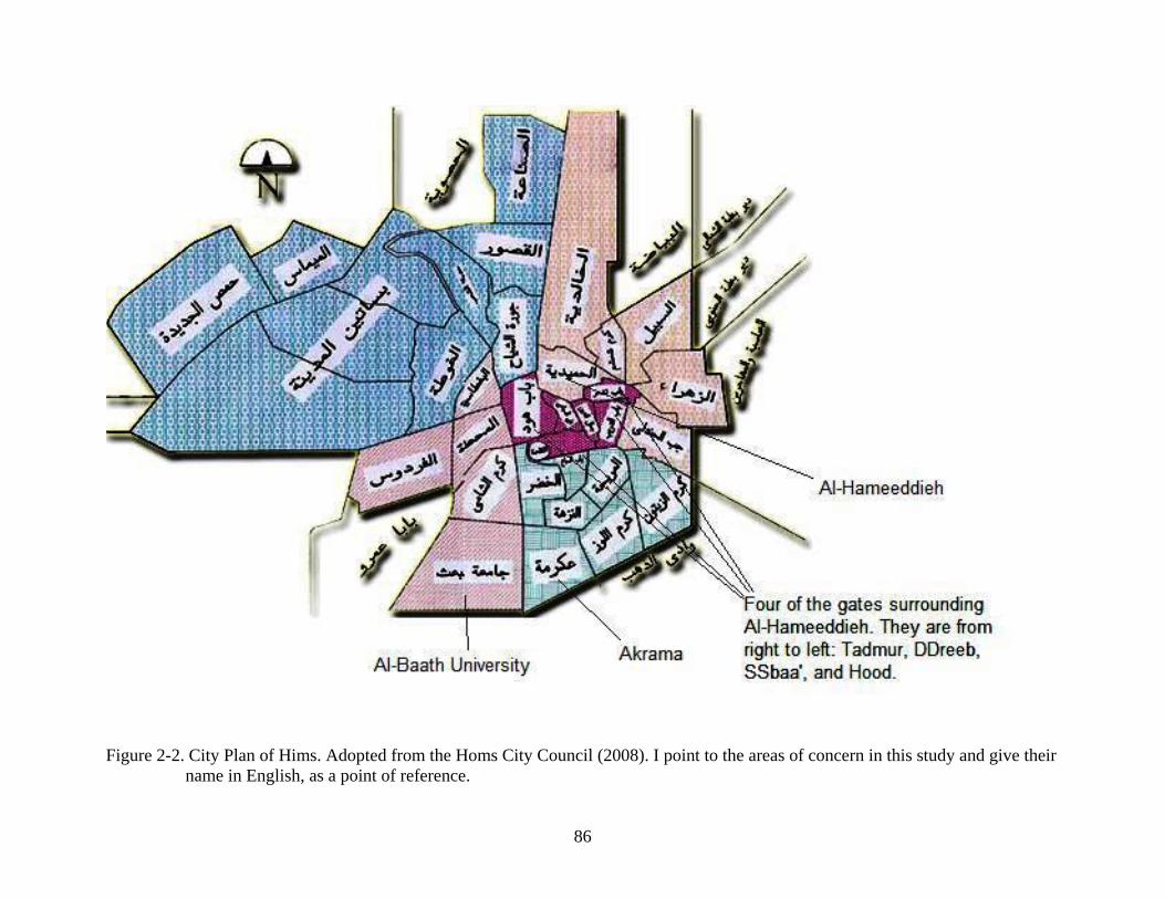
86
Figure 2-2. City Plan of Hims. Adopted from the Homs City Council (2008). I point to the areas of concern in this study and give their name in English, as a point of reference.

87
CHAPTER 3 THEORETICAL ANALYSIS
3.1 Introduction to the Theoretical Analysis of the Data
Having discussed the working mechanism of the GLA and its advantages over other
approaches to language variation, I will now present the theoretical analysis that motivated this
study. In the GLA and OT, mainly linguistic, phonetic, phonological, morphological, or syntactic
constraints have been taken into account. Thus, to answer the question about how we could
model sociolinguistic variation using these theoretical frameworks and how we could intersect
the social and the linguistic within the same theory or framework, I propose a number of social
constraints and integrate them into the GLA. These constraints will interact with linguistic
markedness and faithfulness constraints that militate against a certain sound or against the
change of a certain sound respectively.
I will start with modeling the observed variation between [q] and [] in the speech of rural
migrant speakers to the city of Hims, proposing and implementing linguistic constraints and
social constraints that are pertinent to this variation, stating the motivation behind them. I will
show examples with and without the intersection of social constraints with phonological
constraints. This will allow the reader to see different results when social constraints are
involved, results that match or approximate real life occurrences. The inclusion of social
constraints in the computation will provide an explanation of the observed intra- and inter-
speaker variation (i.e., the speakers’ different grammars within the same social group or
community or among different social groups).
Then, I will take on the constraints that are required to model the stable variation we
observe with respect to [t] and [s] and [d] and [z] in the speech of all speakers. With stable
variation, I mean that certain words are consistently pronounced with one of the four variants and

88
never with one of the other variants; thus, the four variants are not interchangeable. I will explain
this point more when I explore these four variants in depth in Section 3.3. We will observe later
on that the latter variation is led by different factors from the former variation, in that the
interaction between social constraints and linguistic constraints does not make a difference. What
are at work in this type of variation are mainly faithfulness constraints that militate against the
change of some sound features to maintain contrast in pronunciation among various words that
historically stemmed from SA [] and [].
3.2 Modeling Variation between [q] and []
In this section, I will first explore the linguistic constraints that are required to account for
the observed variation between [q] and [] in the speech of rural migrant speakers to the city of
Hims. Then, I will propose a number of social constraints and intersect them with the proposed
linguistic constraints to account for the intra- and interpersonal variation observed in my data.
The proposition of social constraints and intersecting them with linguistic constraints will show
that the social and linguistic can be intertwined in one linguistic theory. It will also show that
social factors do influence our choice of a grammar at a certain time and place. Above all, social
constraints determine the degree of intra- and interpersonal speech variation, the ranking value of
other constraints, and the percentages of the occurrence of each of [q] and []. They provide
explanation of the speakers’ different grammars and give us expectations on what the speech of a
certain speaker or group of speakers should sound like. In this study, we will see tangible
evidence of the influence of social constraints on our grammar, evidence that makes them not
only influential but also part of our grammar.
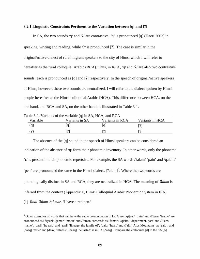
89
3.2.1 Linguistic Constraints Pertinent to the Variation between [q] and []
In SA, the two sounds /q/ and // are contrastive; /q/ is pronounced [q] (Haeri 2003) in
speaking, writing and reading, while // is pronounced []. The case is similar in the
original/native dialect of rural migrant speakers to the city of Hims, which I will refer to
hereafter as the rural colloquial Arabic (RCA). Thus, in RCA, /q/ and // are also two contrastive
sounds; each is pronounced as [q] and [] respectively. In the speech of original/native speakers
of Hims, however, these two sounds are neutralized. I will refer to the dialect spoken by Himsi
people hereafter as the Himsi colloquial Arabic (HCA). This difference between HCA, on the
one hand, and RCA and SA, on the other hand, is illustrated in Table 3-1.
Table 3-1. Variants of the variable (q) in SA, HCA, and RCA Variable Variants in SA Variants in RCA Variants in HCA (q) [q] [q] [] () [] [] []
The absence of the [q] sound in the speech of Himsi speakers can be considered an
indication of the absence of /q/ form their phonemic inventory. In other words, only the phoneme
// is present in their phonemic repertoire. For example, the SA words /alam/ ‘pain’ and /qalam/
‘pen’ are pronounced the same in the Himsi dialect, [alam]8. Where the two words are
phonologically distinct in SA and RCA, they are neutralized in HCA. The meaning of alam is
inferred from the context (Appendix F, Himsi Colloquial Arabic Phonemic System in IPA):
(1) indi alam aħmar. ‘I have a red pen.’ 8 Other examples of words that can have the same pronunciation in HCA are: /qiaar/ ‘train’ and /iaar/ ‘frame’ are pronounced as [iaar]; /qamar/ ‘moon’ and /amar/ ‘ordered’ as [amar]; /qisim/ ‘department, part’ and /isim/ ‘name’; [qaal] ‘he said’ and [aal] ‘lineage, the family of’; /qalb/ ‘heart’ and /alb/ ‘Alps Mountains’ as [alb]; and [daaq] ‘taste’ and [daa] ‘illness’. [daaq] ‘he tasted’ is in SA [aaq]. Compare the colloquial [d] to the SA [].
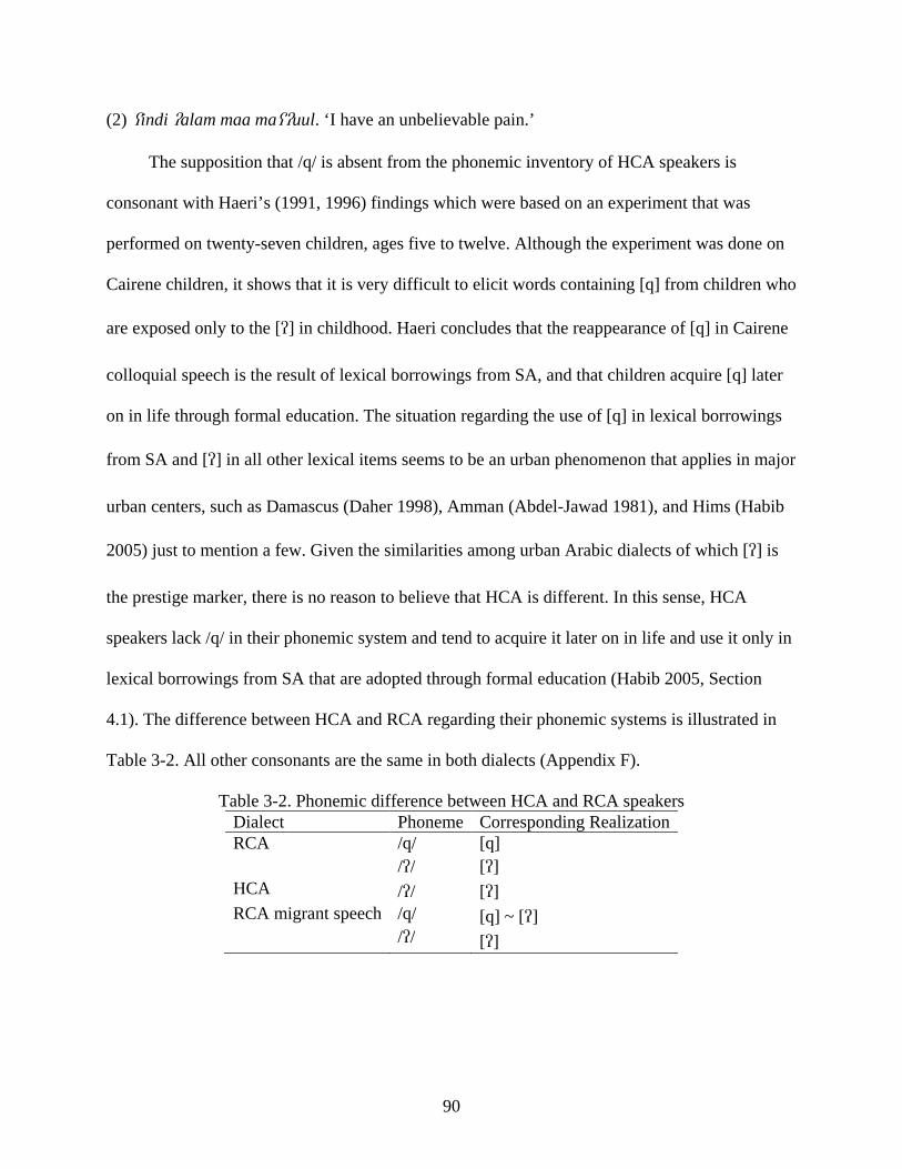
90
(2) indi alam maa mauul. ‘I have an unbelievable pain.’
The supposition that /q/ is absent from the phonemic inventory of HCA speakers is
consonant with Haeri’s (1991, 1996) findings which were based on an experiment that was
performed on twenty-seven children, ages five to twelve. Although the experiment was done on
Cairene children, it shows that it is very difficult to elicit words containing [q] from children who
are exposed only to the [] in childhood. Haeri concludes that the reappearance of [q] in Cairene
colloquial speech is the result of lexical borrowings from SA, and that children acquire [q] later
on in life through formal education. The situation regarding the use of [q] in lexical borrowings
from SA and [] in all other lexical items seems to be an urban phenomenon that applies in major
urban centers, such as Damascus (Daher 1998), Amman (Abdel-Jawad 1981), and Hims (Habib
2005) just to mention a few. Given the similarities among urban Arabic dialects of which [] is
the prestige marker, there is no reason to believe that HCA is different. In this sense, HCA
speakers lack /q/ in their phonemic system and tend to acquire it later on in life and use it only in
lexical borrowings from SA that are adopted through formal education (Habib 2005, Section
4.1). The difference between HCA and RCA regarding their phonemic systems is illustrated in
Table 3-2. All other consonants are the same in both dialects (Appendix F).
Table 3-2. Phonemic difference between HCA and RCA speakers Dialect Phoneme Corresponding Realization RCA /q/
// [q] []
HCA // [] RCA migrant speech /q/
// [q] ~ [] []
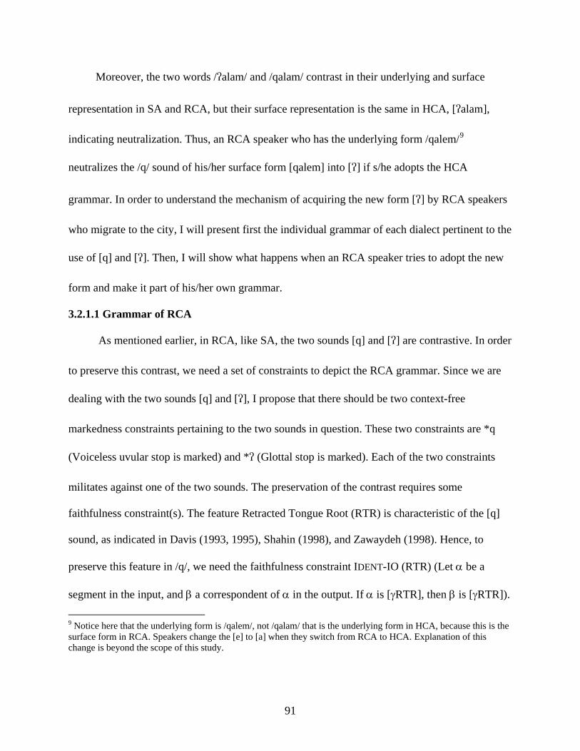
91
Moreover, the two words /alam/ and /qalam/ contrast in their underlying and surface
representation in SA and RCA, but their surface representation is the same in HCA, [alam],
indicating neutralization. Thus, an RCA speaker who has the underlying form /qalem/9
neutralizes the /q/ sound of his/her surface form [qalem] into [] if s/he adopts the HCA
grammar. In order to understand the mechanism of acquiring the new form [] by RCA speakers
who migrate to the city, I will present first the individual grammar of each dialect pertinent to the
use of [q] and []. Then, I will show what happens when an RCA speaker tries to adopt the new
form and make it part of his/her own grammar.
3.2.1.1 Grammar of RCA
As mentioned earlier, in RCA, like SA, the two sounds [q] and [] are contrastive. In order
to preserve this contrast, we need a set of constraints to depict the RCA grammar. Since we are
dealing with the two sounds [q] and [], I propose that there should be two context-free
markedness constraints pertaining to the two sounds in question. These two constraints are *q
(Voiceless uvular stop is marked) and * (Glottal stop is marked). Each of the two constraints
militates against one of the two sounds. The preservation of the contrast requires some
faithfulness constraint(s). The feature Retracted Tongue Root (RTR) is characteristic of the [q]
sound, as indicated in Davis (1993, 1995), Shahin (1998), and Zawaydeh (1998). Hence, to
preserve this feature in /q/, we need the faithfulness constraint IDENT-IO (RTR) (Let α be a
segment in the input, and β a correspondent of α in the output. If α is [γRTR], then β is [γRTR]).
9 Notice here that the underlying form is /qalem/, not /qalam/ that is the underlying form in HCA, because this is the surface form in RCA. Speakers change the [e] to [a] when they switch from RCA to HCA. Explanation of this change is beyond the scope of this study.
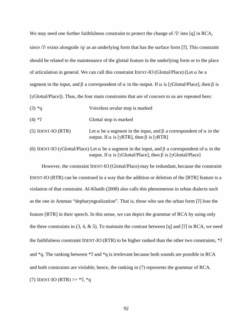
92
We may need one further faithfulness constraint to protect the change of // into [q] in RCA,
since // exists alongside /q/ as an underlying form that has the surface form []. This constraint
should be related to the maintenance of the glottal feature in the underlying form or to the place
of articulation in general. We can call this constraint IDENT-IO (Glottal/Place) (Let α be a
segment in the input, and β a correspondent of α in the output. If α is [γGlottal/Place], then β is
[γGlottal/Place]). Thus, the four main constraints that are of concern to us are repeated here:
(3) *q Voiceless uvular stop is marked
(4) * Glottal stop is marked
(5) IDENT-IO (RTR) Let α be a segment in the input, and β a correspondent of α in the output. If α is [γRTR], then β is [γRTR] (6) IDENT-IO (γGlottal/Place) Let α be a segment in the input, and β a correspondent of α in the output. If α is [γGlottal/Place], then β is [γGlottal/Place]
However, the constraint IDENT-IO (Glottal/Place) may be redundant, because the constraint
IDENT-IO (RTR) can be construed in a way that the addition or deletion of the [RTR] feature is a
violation of that constraint. Al-Khatib (2008) also calls this phenomenon in urban dialects such
as the one in Amman “depharyngealization”. That is, those who use the urban form [] lose the
feature [RTR] in their speech. In this sense, we can depict the grammar of RCA by using only
the three constraints in (3, 4, & 5). To maintain the contrast between [q] and [] in RCA, we need
the faithfulness constraint IDENT-IO (RTR) to be higher ranked than the other two constraints, *
and *q. The ranking between * and *q is irrelevant because both sounds are possible in RCA
and both constraints are violable; hence, the ranking in (7) represents the grammar of RCA.
(7) IDENT-IO (RTR) >> *, *q
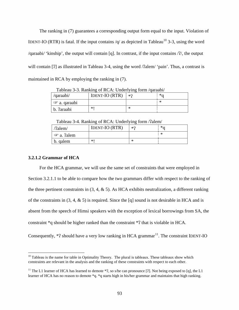
93
The ranking in (7) guarantees a corresponding output form equal to the input. Violation of
IDENT-IO (RTR) is fatal. If the input contains /q/ as depicted in Tableau10 3-3, using the word
/qaraabi/ ‘kinship’, the output will contain [q]. In contrast, if the input contains //, the output
will contain [] as illustrated in Tableau 3-4, using the word /alem/ ‘pain’. Thus, a contrast is
maintained in RCA by employing the ranking in (7).
Tableau 3-3. Ranking of RCA: Underlying form /qaraabi/ /qaraabi/ IDENT-IO (RTR) * *q ☞ a. qaraabi * b. araabi *! *
Tableau 3-4. Ranking of RCA: Underlying form /alem/
/alem/ IDENT-IO (RTR) * *q ☞ a. alem * b. qalem *! *
3.2.1.2 Grammar of HCA
For the HCA grammar, we will use the same set of constraints that were employed in
Section 3.2.1.1 to be able to compare how the two grammars differ with respect to the ranking of
the three pertinent constraints in (3, 4, & 5). As HCA exhibits neutralization, a different ranking
of the constraints in (3, 4, & 5) is required. Since the [q] sound is not desirable in HCA and is
absent from the speech of Himsi speakers with the exception of lexical borrowings from SA, the
constraint *q should be higher ranked than the constraint * that is violable in HCA.
Consequently, * should have a very low ranking in HCA grammar11. The constraint IDENT-IO
10 Tableau is the name for table in Optimality Theory. The plural is tableaux. These tableaux show which constraints are relevant in the analysis and the ranking of these constraints with respect to each other.
11 The L1 learner of HCA has learned to demote *, so s/he can pronounce []. Not being exposed to [q], the L1 learner of HCA has no reason to demote *q. *q starts high in his/her grammar and maintains that high ranking.
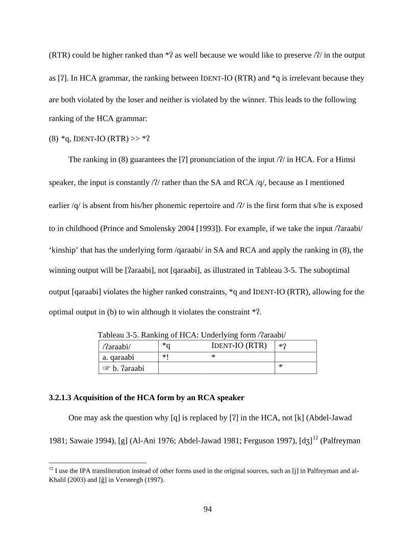
94
(RTR) could be higher ranked than * as well because we would like to preserve // in the output
as []. In HCA grammar, the ranking between IDENT-IO (RTR) and *q is irrelevant because they
are both violated by the loser and neither is violated by the winner. This leads to the following
ranking of the HCA grammar:
(8) *q, IDENT-IO (RTR) >> *
The ranking in (8) guarantees the [] pronunciation of the input // in HCA. For a Himsi
speaker, the input is constantly // rather than the SA and RCA /q/, because as I mentioned
earlier /q/ is absent from his/her phonemic repertoire and // is the first form that s/he is exposed
to in childhood (Prince and Smolensky 2004 [1993]). For example, if we take the input /araabi/
‘kinship’ that has the underlying form /qaraabi/ in SA and RCA and apply the ranking in (8), the
winning output will be [araabi], not [qaraabi], as illustrated in Tableau 3-5. The suboptimal
output [qaraabi] violates the higher ranked constraints, *q and IDENT-IO (RTR), allowing for the
optimal output in (b) to win although it violates the constraint *.
Tableau 3-5. Ranking of HCA: Underlying form /araabi/ /araabi/ *q IDENT-IO (RTR) * a. qaraabi *! * ☞ b. araabi *
3.2.1.3 Acquisition of the HCA form by an RCA speaker
One may ask the question why [q] is replaced by [] in the HCA, not [k] (Abdel-Jawad
1981; Sawaie 1994), [g] (Al-Ani 1976; Abdel-Jawad 1981; Ferguson 1997), [d]12 (Palfreyman
12 I use the IPA transliteration instead of other forms used in the original sources, such as [j] in Palfreyman and al-Khalil (2003) and [g] in Versteegh (1997).
95
and al-Khalil 2003; Versteegh 1997:149), or its more fronted variant [dz] (Versteegh 1997:149).
/g/ used to exist in Old Arabic, but with time, it was lost for another place of articulation,
palatoalveolar affricate /d/ (Moscati, Spitaler, Ullendorff, and von Soden 1964). Nowadays, [g]
still exists in some Bedouin or village dialects, where it replaces the /q/ sound (Abdel-Jawad
1981; Ferguson, 1997). Because [], not [k], [g], [d], [dz], or [q], is the sound used in HCA, we
can assume that if a set of context-free markedness constraints exist for all the unused sounds in
HCA, these constraints will be ranked higher than * in HCA, as illustrated in (9).
(9) *k, *g, *d, *dz, *q >> *
On the other hand, in the RCA dialect [q] and [] have equal weight because they are
contrastive. Thus, the same set of context-free markedness constraints will be ranked in RCA as
in (10) because the other four sounds do not occur in RCA.
(10) *k, *g, *d, *dz >> *, *q
Since neither dialect allows [k], [g], [d] or [dz] as a replacement for [q], I do not include
the constraints *k, *g, *d, and *dz in the ranking of constraints for each dialect. In both dialects,
these four constraints are undominated. Thus, we should not concern ourselves with them. These
constraints could be used to describe changes that occur in other Arabic dialects that make use of
the sounds [k], [g], [d], or [dz] in place of [q]. Our main concern here is the change of grammar
that occurs as a result of the switch from RCA to HCA. Since the change is taking place from the
RCA form to the HCA form, there must be some process of reranking of the three constraints in
the RCA grammar (IDENT-IO (RTR) >> *q, *) for an RCA speaker to sound like an HCA
speaker. Because the change is taking place from the village dialect to the city dialect, the
96
assumed input is the surface form of the RCA dialect, in accordance with Prince and
Smolensky’s (2004 [1993]) idea of Lexicon Optimization, which is an elaboration on Stampe’s
(1972) idea. Lexicon Optimization holds that the input should be the form closest to the surface
form that a child is first exposed to, unless there is evidence otherwise as from alternations, and
it is this input that undergoes change.
It is worth noting here that the acquisition of the HCA form does not necessarily involve
complete acquisition of the HCA grammar because of the difference in input form for an HCA
speaker and an RCA speaker. It also seems that the RCA ranking (IDENT-IO (RTR) >> *, *q)
promotes faithfulness over markedness to maintain the contrast between [q] and [], whereas the
HCA ranking (*q, IDENT-IO (RTR) >> *) partially promotes markedness to avoid the marked
sound [q]. This implies that rural speakers who attempt to learn the new form [] of the HCA
dialect are inclined towards the unmarked. It may appear to the observer at first sight that the
variation observed in the speech of rural migrant speakers is only a kind of change towards the
unmarked.
However, the situation is more complex than it may appear. It is true that the variation
observed in the speech of rural migrant speakers to the city of Hims is an indication of an attempt
on the part of the learners to acquire the HCA grammar. However, the degree of variation differs
from one speaker to another and from one group of speakers to another. The degree of use of the
new form may range from zero to one hundred percent based on a number of social factors, such
as age, gender, social class, and residential area. Before delving into the social influence on our
choice of a grammar, let us portray what we mean by complete acquisition of or competence in
the HCA form by an RCA speaker. In other words, let us examine what results from the
interaction of the two grammars.
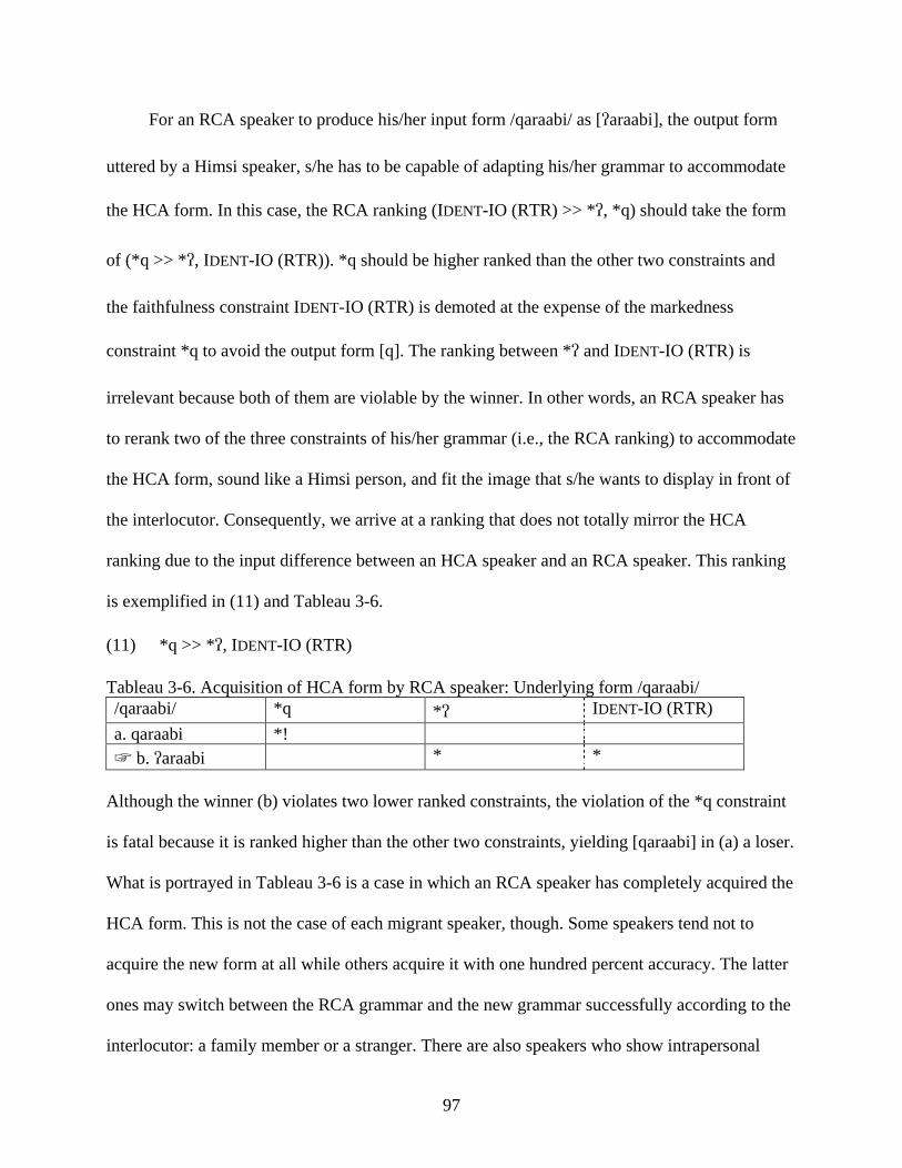
97
For an RCA speaker to produce his/her input form /qaraabi/ as [araabi], the output form
uttered by a Himsi speaker, s/he has to be capable of adapting his/her grammar to accommodate
the HCA form. In this case, the RCA ranking (IDENT-IO (RTR) >> *, *q) should take the form
of (*q >> *, IDENT-IO (RTR)). *q should be higher ranked than the other two constraints and
the faithfulness constraint IDENT-IO (RTR) is demoted at the expense of the markedness
constraint *q to avoid the output form [q]. The ranking between * and IDENT-IO (RTR) is
irrelevant because both of them are violable by the winner. In other words, an RCA speaker has
to rerank two of the three constraints of his/her grammar (i.e., the RCA ranking) to accommodate
the HCA form, sound like a Himsi person, and fit the image that s/he wants to display in front of
the interlocutor. Consequently, we arrive at a ranking that does not totally mirror the HCA
ranking due to the input difference between an HCA speaker and an RCA speaker. This ranking
is exemplified in (11) and Tableau 3-6.
(11) *q >> *, IDENT-IO (RTR) Tableau 3-6. Acquisition of HCA form by RCA speaker: Underlying form /qaraabi/ /qaraabi/ *q * IDENT-IO (RTR) a. qaraabi *! ☞ b. araabi * *
Although the winner (b) violates two lower ranked constraints, the violation of the *q constraint
is fatal because it is ranked higher than the other two constraints, yielding [qaraabi] in (a) a loser.
What is portrayed in Tableau 3-6 is a case in which an RCA speaker has completely acquired the
HCA form. This is not the case of each migrant speaker, though. Some speakers tend not to
acquire the new form at all while others acquire it with one hundred percent accuracy. The latter
ones may switch between the RCA grammar and the new grammar successfully according to the
interlocutor: a family member or a stranger. There are also speakers who show intrapersonal
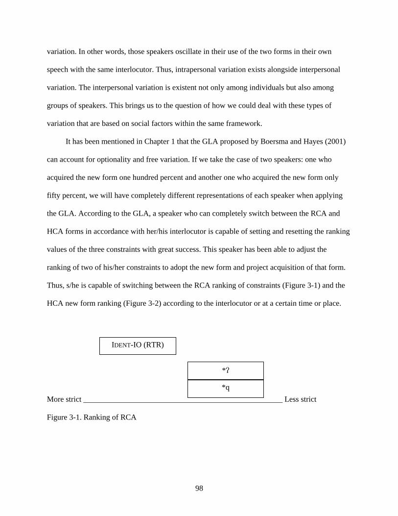
98
variation. In other words, those speakers oscillate in their use of the two forms in their own
speech with the same interlocutor. Thus, intrapersonal variation exists alongside interpersonal
variation. The interpersonal variation is existent not only among individuals but also among
groups of speakers. This brings us to the question of how we could deal with these types of
variation that are based on social factors within the same framework.
It has been mentioned in Chapter 1 that the GLA proposed by Boersma and Hayes (2001)
can account for optionality and free variation. If we take the case of two speakers: one who
acquired the new form one hundred percent and another one who acquired the new form only
fifty percent, we will have completely different representations of each speaker when applying
the GLA. According to the GLA, a speaker who can completely switch between the RCA and
HCA forms in accordance with her/his interlocutor is capable of setting and resetting the ranking
values of the three constraints with great success. This speaker has been able to adjust the
ranking of two of his/her constraints to adopt the new form and project acquisition of that form.
Thus, s/he is capable of switching between the RCA ranking of constraints (Figure 3-1) and the
HCA new form ranking (Figure 3-2) according to the interlocutor or at a certain time or place.
More strict ___________________________________________________ Less strict
Figure 3-1. Ranking of RCA
IDENT-IO (RTR)
*
*q
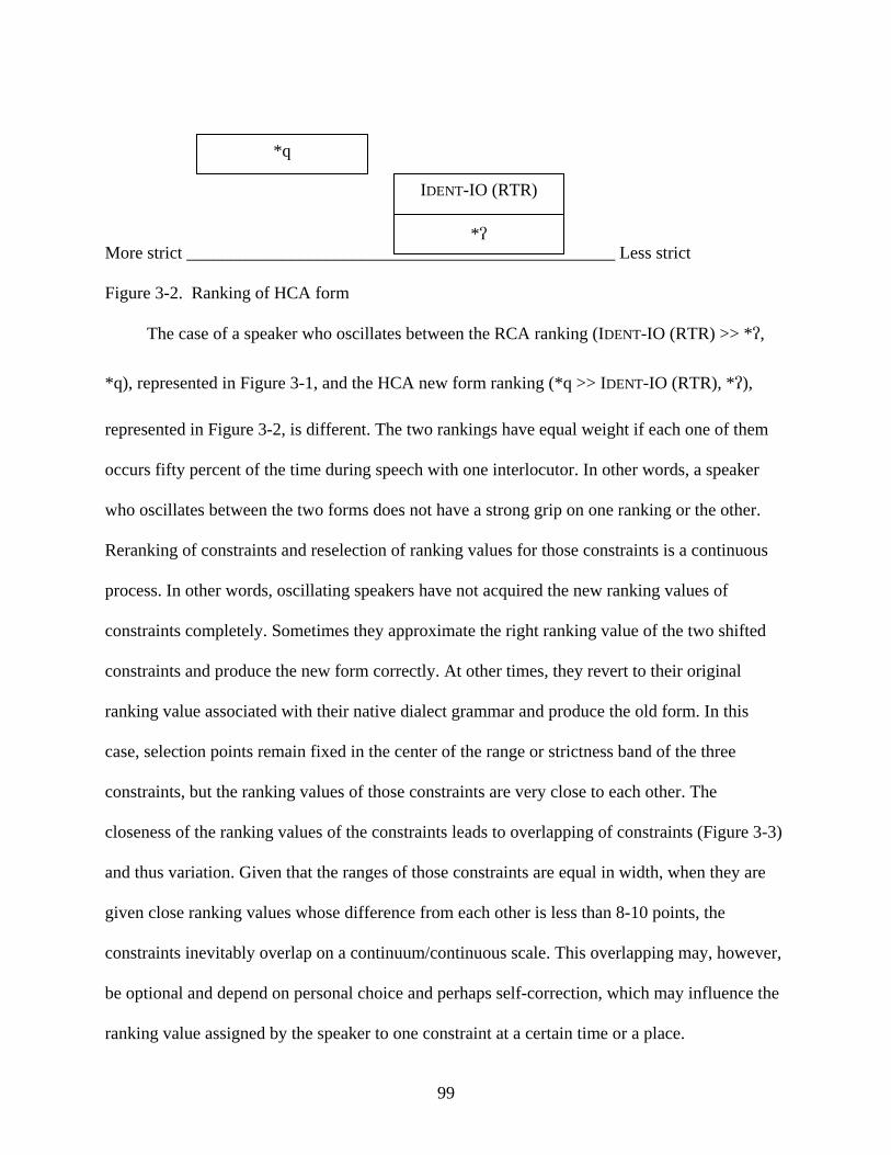
99
More strict _________________________________________________ Less strict
Figure 3-2. Ranking of HCA form
The case of a speaker who oscillates between the RCA ranking (IDENT-IO (RTR) >> *,
*q), represented in Figure 3-1, and the HCA new form ranking (*q >> IDENT-IO (RTR), *),
represented in Figure 3-2, is different. The two rankings have equal weight if each one of them
occurs fifty percent of the time during speech with one interlocutor. In other words, a speaker
who oscillates between the two forms does not have a strong grip on one ranking or the other.
Reranking of constraints and reselection of ranking values for those constraints is a continuous
process. In other words, oscillating speakers have not acquired the new ranking values of
constraints completely. Sometimes they approximate the right ranking value of the two shifted
constraints and produce the new form correctly. At other times, they revert to their original
ranking value associated with their native dialect grammar and produce the old form. In this
case, selection points remain fixed in the center of the range or strictness band of the three
constraints, but the ranking values of those constraints are very close to each other. The
closeness of the ranking values of the constraints leads to overlapping of constraints (Figure 3-3)
and thus variation. Given that the ranges of those constraints are equal in width, when they are
given close ranking values whose difference from each other is less than 8-10 points, the
constraints inevitably overlap on a continuum/continuous scale. This overlapping may, however,
be optional and depend on personal choice and perhaps self-correction, which may influence the
ranking value assigned by the speaker to one constraint at a certain time or a place.
IDENT-IO (RTR)
*
*q
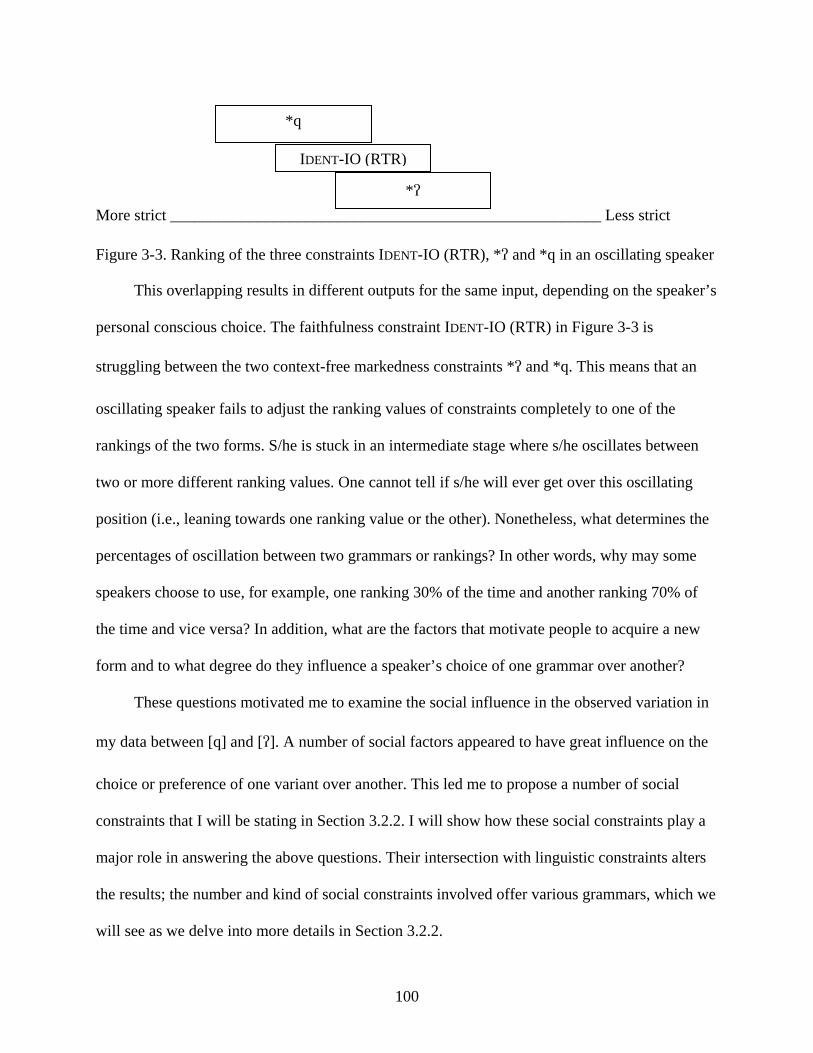
100
More strict ______________________________________________________ Less strict
Figure 3-3. Ranking of the three constraints IDENT-IO (RTR), * and *q in an oscillating speaker
This overlapping results in different outputs for the same input, depending on the speaker’s
personal conscious choice. The faithfulness constraint IDENT-IO (RTR) in Figure 3-3 is
struggling between the two context-free markedness constraints * and *q. This means that an
oscillating speaker fails to adjust the ranking values of constraints completely to one of the
rankings of the two forms. S/he is stuck in an intermediate stage where s/he oscillates between
two or more different ranking values. One cannot tell if s/he will ever get over this oscillating
position (i.e., leaning towards one ranking value or the other). Nonetheless, what determines the
percentages of oscillation between two grammars or rankings? In other words, why may some
speakers choose to use, for example, one ranking 30% of the time and another ranking 70% of
the time and vice versa? In addition, what are the factors that motivate people to acquire a new
form and to what degree do they influence a speaker’s choice of one grammar over another?
These questions motivated me to examine the social influence in the observed variation in
my data between [q] and []. A number of social factors appeared to have great influence on the
choice or preference of one variant over another. This led me to propose a number of social
constraints that I will be stating in Section 3.2.2. I will show how these social constraints play a
major role in answering the above questions. Their intersection with linguistic constraints alters
the results; the number and kind of social constraints involved offer various grammars, which we
will see as we delve into more details in Section 3.2.2.
IDENT-IO (RTR)
*
*q
101
3.2.2 Social Constraints Pertinent to the Variation between [q] and []
In this section, I propose a number of social constraints based on social factors that have
been often investigated and stressed as essential factors in language variation and change (e.g.,
Labov 2001). Among these factors are age, gender, residential area, and social class (e.g., Labov
1966, 1972a; Milroy 1980; Eckert 1989, 1991). I choose these factors because I believe that they
play a major role in this study, and they are applicable to other studies and languages or dialects.
In the following list of constraints, each of the social factors included in the study is split
into four social constraints. Of course, this division of constraints may differ in other languages
or when dealing with different variables. As I am dealing here with the variation between [q] and
[], I state the social constraints that can restrict the use of each of these two sounds. For
example, the category of gender consists of males and females who can either use [q] or []. This
motivates the division of the gender social factor into four separate gender constraints, each
stating that one of the sounds is socially marked when used by one of the genders. Thus, gender
is factored first into males and females. Then, males are factored into marked usage of [q] and
marked usage of []. Females are factored in the same way, resulting in four distinct social
constraints pertaining to gender and to the use of [q] and []. Each social factor is treated in the
same way, resulting in sixteen different social constraints. Each social factor consists of two
categories, and each category is split into those to whom [q] is marked socially and those to
whom [] is marked socially. We need a balanced number and type of constraints for each social
factor, even in cases in which certain constraints are inactive or not activated by a certain
individual or a group of individuals because the theory should be as general as possible. In
addition, the social values of linguistic sounds may differ from one speaker to another or from
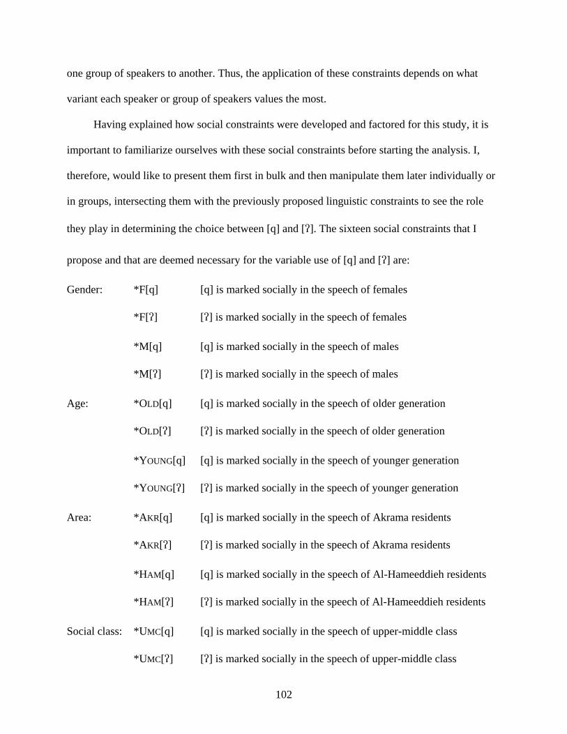
102
one group of speakers to another. Thus, the application of these constraints depends on what
variant each speaker or group of speakers values the most.
Having explained how social constraints were developed and factored for this study, it is
important to familiarize ourselves with these social constraints before starting the analysis. I,
therefore, would like to present them first in bulk and then manipulate them later individually or
in groups, intersecting them with the previously proposed linguistic constraints to see the role
they play in determining the choice between [q] and []. The sixteen social constraints that I
propose and that are deemed necessary for the variable use of [q] and [] are:
Gender: *F[q] [q] is marked socially in the speech of females
*F[] [] is marked socially in the speech of females
*M[q] [q] is marked socially in the speech of males
*M[] [] is marked socially in the speech of males
Age: *OLD[q] [q] is marked socially in the speech of older generation
*OLD[] [] is marked socially in the speech of older generation
*YOUNG[q] [q] is marked socially in the speech of younger generation
*YOUNG[] [] is marked socially in the speech of younger generation
Area: *AKR[q] [q] is marked socially in the speech of Akrama residents
*AKR[] [] is marked socially in the speech of Akrama residents
*HAM[q] [q] is marked socially in the speech of Al-Hameeddieh residents
*HAM[] [] is marked socially in the speech of Al-Hameeddieh residents
Social class: *UMC[q] [q] is marked socially in the speech of upper-middle class
*UMC[] [] is marked socially in the speech of upper-middle class
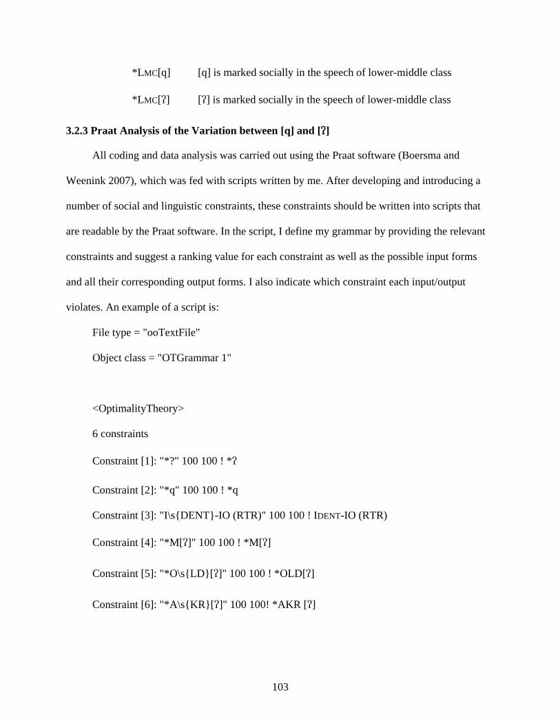
103
*LMC[q] [q] is marked socially in the speech of lower-middle class
*LMC[] [] is marked socially in the speech of lower-middle class
3.2.3 Praat Analysis of the Variation between [q] and []
All coding and data analysis was carried out using the Praat software (Boersma and
Weenink 2007), which was fed with scripts written by me. After developing and introducing a
number of social and linguistic constraints, these constraints should be written into scripts that
are readable by the Praat software. In the script, I define my grammar by providing the relevant
constraints and suggest a ranking value for each constraint as well as the possible input forms
and all their corresponding output forms. I also indicate which constraint each input/output
violates. An example of a script is:
File type = "ooTextFile"
Object class = "OTGrammar 1"
<OptimalityTheory>
6 constraints
Constraint [1]: "*?" 100 100 ! *
Constraint [2]: "*q" 100 100 ! *q
Constraint [3]: "I\s{DENT}-IO (RTR)" 100 100 ! IDENT-IO (RTR)
Constraint [4]: "*M[]" 100 100 ! *M[]
Constraint [5]: "*O\s{LD}[]" 100 100 ! *OLD[]
Constraint [6]: "*A\s{KR}[]" 100 100! *AKR []
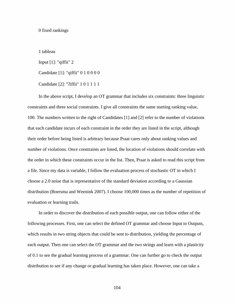
104
0 fixed rankings
1 tableau
Input [1]: "qiffii" 2
Candidate [1]: "qiffii" 0 1 0 0 0 0
Candidate [2]: "iffii" 1 0 1 1 1 1
In the above script, I develop an OT grammar that includes six constraints: three linguistic
constraints and three social constraints. I give all constraints the same starting ranking value,
100. The numbers written to the right of Candidates [1] and [2] refer to the number of violations
that each candidate incurs of each constraint in the order they are listed in the script, although
their order before being listed is arbitrary because Praat cares only about ranking values and
number of violations. Once constraints are listed, the location of violations should correlate with
the order in which these constraints occur in the list. Then, Praat is asked to read this script from
a file. Since my data is variable, I follow the evaluation process of stochastic OT in which I
choose a 2.0 noise that is representative of the standard deviation according to a Gaussian
distribution (Boersma and Weenink 2007). I choose 100,000 times as the number of repetition of
evaluation or learning trails.
In order to discover the distribution of each possible output, one can follow either of the
following processes. First, one can select the defined OT grammar and choose Input to Outputs,
which results in two string objects that could be sent to distribution, yielding the percentage of
each output. Then one can select the OT grammar and the two strings and learn with a plasticity
of 0.1 to see the gradual learning process of a grammar. One can further go to check the output
distribution to see if any change or gradual learning has taken place. However, one can take a
105
shortcut to grammar learning (Boersma and Weenink 2007) by skipping the strings step and
immediately choose to go to pair distribution from selecting the OT grammar, then select the OT
grammar and the pair distribution and learn with a plasticity of 0.1. This not only allows us to
observe learning but also to find out the output distribution (i.e., the percentage of the occurrence
of each variant) by choosing to go to strings from pair distribution and then from strings to
distribution. Consequently, we will get input distribution and output distribution. This process is
applied to a number of grammars defined by me to see how social constraints could affect our
choice of a grammar at a certain time and place and the degree to which they affect our
grammars and the ranking values as well as the rankings of other constraints.
Because I am interested in modeling real life variation, after applying the previous process
I chose to apply learning from partial outputs that become inputs for speakers. I select the OT
grammar and the output distribution or the output string and learn from partial outputs. The
motivation behind this type of learning is that speakers are constantly exposed to variation in the
output they receive as input. This should definitely influence their learning process and their next
set of outputs. In other words, it will influence the percentages of the occurrence of each of the
variants in their speech. The complete process of learning from partial outputs is that we first
read an OT grammar from a script file prepared and defined by the author, select it, and go to
pair distribution. Then, we select the pair distribution that appears in the object window and go to
strings. We can select only the output string and go to output distribution. This output
distribution is selected with the previously defined OT grammar, and we let Praat learn from
partial outputs with a plasticity of 0.1 and a number of learning trails set to 100,000. In order to
explain this learning process, I will present a number of examples and show how it can model
real life occurrences of the variants under investigation. It is worth noting here that the examples
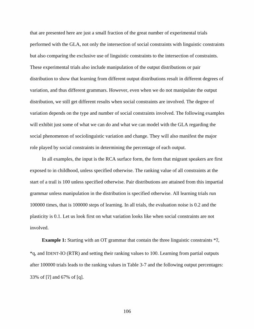
106
that are presented here are just a small fraction of the great number of experimental trials
performed with the GLA, not only the intersection of social constraints with linguistic constraints
but also comparing the exclusive use of linguistic constraints to the intersection of constraints.
These experimental trials also include manipulation of the output distributions or pair
distribution to show that learning from different output distributions result in different degrees of
variation, and thus different grammars. However, even when we do not manipulate the output
distribution, we still get different results when social constraints are involved. The degree of
variation depends on the type and number of social constraints involved. The following examples
will exhibit just some of what we can do and what we can model with the GLA regarding the
social phenomenon of sociolinguistic variation and change. They will also manifest the major
role played by social constraints in determining the percentage of each output.
In all examples, the input is the RCA surface form, the form that migrant speakers are first
exposed to in childhood, unless specified otherwise. The ranking value of all constraints at the
start of a trail is 100 unless specified otherwise. Pair distributions are attained from this impartial
grammar unless manipulation in the distribution is specified otherwise. All learning trials run
100000 times, that is 100000 steps of learning. In all trials, the evaluation noise is 0.2 and the
plasticity is 0.1. Let us look first on what variation looks like when social constraints are not
involved.
Example 1: Starting with an OT grammar that contain the three linguistic constraints *,
*q, and IDENT-IO (RTR) and setting their ranking values to 100. Learning from partial outputs
after 100000 trials leads to the ranking values in Table 3-7 and the following output percentages:
33% of [] and 67% of [q].
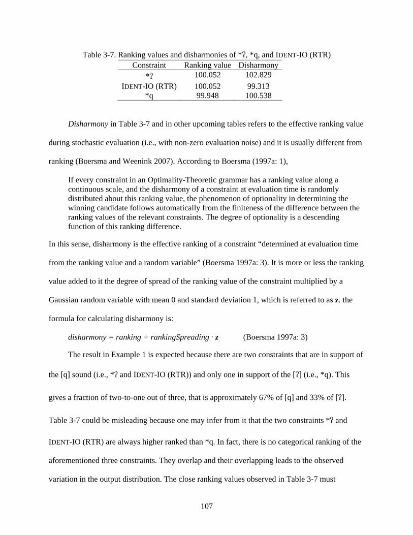
107
Table 3-7. Ranking values and disharmonies of *, *q, and IDENT-IO (RTR) Constraint Ranking value Disharmony
* 100.052 102.829 IDENT-IO (RTR) 100.052 99.313
*q 99.948 100.538
Disharmony in Table 3-7 and in other upcoming tables refers to the effective ranking value
during stochastic evaluation (i.e., with non-zero evaluation noise) and it is usually different from
ranking (Boersma and Weenink 2007). According to Boersma (1997a: 1),
If every constraint in an Optimality-Theoretic grammar has a ranking value along a continuous scale, and the disharmony of a constraint at evaluation time is randomly distributed about this ranking value, the phenomenon of optionality in determining the winning candidate follows automatically from the finiteness of the difference between the ranking values of the relevant constraints. The degree of optionality is a descending function of this ranking difference.
In this sense, disharmony is the effective ranking of a constraint “determined at evaluation time
from the ranking value and a random variable” (Boersma 1997a: 3). It is more or less the ranking
value added to it the degree of spread of the ranking value of the constraint multiplied by a
Gaussian random variable with mean 0 and standard deviation 1, which is referred to as z. the
formula for calculating disharmony is:
disharmony = ranking + rankingSpreading · z (Boersma 1997a: 3)
The result in Example 1 is expected because there are two constraints that are in support of
the [q] sound (i.e., * and IDENT-IO (RTR)) and only one in support of the [] (i.e., *q). This
gives a fraction of two-to-one out of three, that is approximately 67% of [q] and 33% of [].
Table 3-7 could be misleading because one may infer from it that the two constraints * and
IDENT-IO (RTR) are always higher ranked than *q. In fact, there is no categorical ranking of the
aforementioned three constraints. They overlap and their overlapping leads to the observed
variation in the output distribution. The close ranking values observed in Table 3-7 must
108
inevitably result in this overlapping and the non-categorical ranking. The percentages indicate
the number of times the ranking that allows for [q] is chosen and the number of times the ranking
that allows for [] is chosen. But in real life this is not the case. In real life, a person who is
exposed to the overt form [q] 100% of the time, should have 100% pronunciation of [q]; his/her
underlying form, /q/, and surface form [q] should match. There should be a categorical ranking
that determines the grammar of that speaker and identical to the RCA grammar ranking, IDENT-
IO (RTR) >> *q, *. The disparity between real life occurrences and the results of the Praat
software lies in that the software is given equal rankings to the three constraints and two output
candidates for one input (e.g., the outputs [qaraabi] and [araabi] for the input /qaraabi/).
Consequently, the number of constraints that favor one of the two outputs over the other
determines the output distribution or percentages. This situation mirrors Anttila’s SG model for
free variation in which the number of constraints that favors one sound over another determines
the frequency of its occurrence (Anttila 1997a,b, 2002; Anttila and Cho 1998). In Section
1.3.1.3, I mentioned that Anttila’s SG model runs into problems if there is a large disparity in the
output frequencies. The GLA can overcome this problem because of its stochastic process of
learning and the ability to manipulate the ranking values of constraints or the output pair
distribution from which a speaker can learn and mirror his/her environment. The ability to
manipulate the output pair distribution to match real life occurrences can give us the ranking
values of constraints in a speaker or a group of speakers (i.e., the grammar implemented by a
speaker or a group of speakers). Thus, instead of having multiple grammars from which a
speaker chooses one as in the case of SG, the GLA presents one stochastic grammar for each
speaker or group of speakers through manipulation of the pair distribution or the ranking values
of constraints.
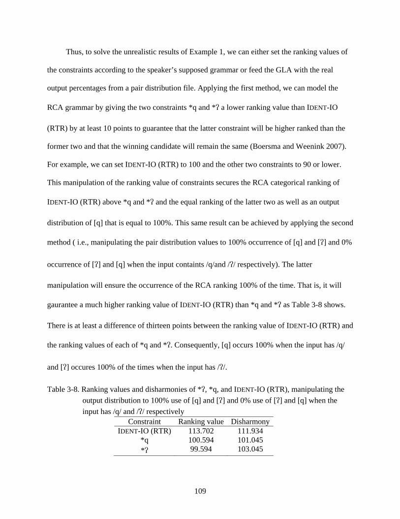
109
Thus, to solve the unrealistic results of Example 1, we can either set the ranking values of
the constraints according to the speaker’s supposed grammar or feed the GLA with the real
output percentages from a pair distribution file. Applying the first method, we can model the
RCA grammar by giving the two constraints *q and * a lower ranking value than IDENT-IO
(RTR) by at least 10 points to guarantee that the latter constraint will be higher ranked than the
former two and that the winning candidate will remain the same (Boersma and Weenink 2007).
For example, we can set IDENT-IO (RTR) to 100 and the other two constraints to 90 or lower.
This manipulation of the ranking value of constraints secures the RCA categorical ranking of
IDENT-IO (RTR) above *q and * and the equal ranking of the latter two as well as an output
distribution of [q] that is equal to 100%. This same result can be achieved by applying the second
method ( i.e., manipulating the pair distribution values to 100% occurrence of [q] and [] and 0%
occurrence of [] and [q] when the input containts /q/and // respectively). The latter
manipulation will ensure the occurrence of the RCA ranking 100% of the time. That is, it will
gaurantee a much higher ranking value of IDENT-IO (RTR) than *q and * as Table 3-8 shows.
There is at least a difference of thirteen points between the ranking value of IDENT-IO (RTR) and
the ranking values of each of *q and *. Consequently, [q] occurs 100% when the input has /q/
and [] occures 100% of the times when the input has //.
Table 3-8. Ranking values and disharmonies of *, *q, and IDENT-IO (RTR), manipulating the output distribution to 100% use of [q] and [] and 0% use of [] and [q] when the input has /q/ and // respectively
Constraint Ranking value Disharmony IDENT-IO (RTR) 113.702 111.934
*q 100.594 101.045 * 99.594 103.045
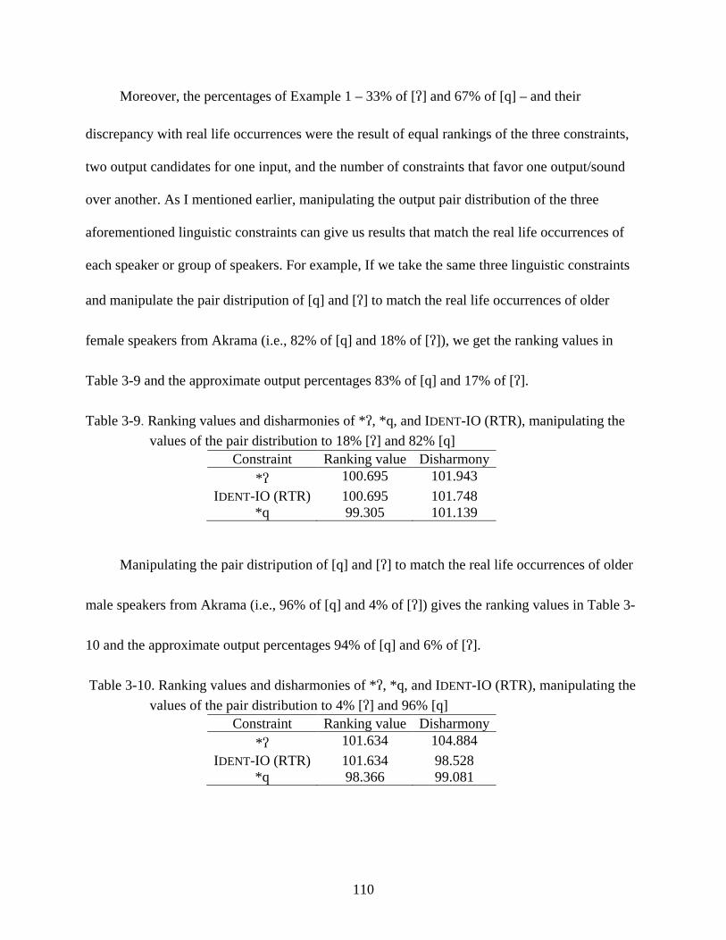
110
Moreover, the percentages of Example 1 – 33% of [] and 67% of [q] – and their
discrepancy with real life occurrences were the result of equal rankings of the three constraints,
two output candidates for one input, and the number of constraints that favor one output/sound
over another. As I mentioned earlier, manipulating the output pair distribution of the three
aforementioned linguistic constraints can give us results that match the real life occurrences of
each speaker or group of speakers. For example, If we take the same three linguistic constraints
and manipulate the pair distripution of [q] and [] to match the real life occurrences of older
female speakers from Akrama (i.e., 82% of [q] and 18% of []), we get the ranking values in
Table 3-9 and the approximate output percentages 83% of [q] and 17% of [].
Table 3-9. Ranking values and disharmonies of *, *q, and IDENT-IO (RTR), manipulating the values of the pair distribution to 18% [] and 82% [q]
Constraint Ranking value Disharmony * 100.695 101.943
IDENT-IO (RTR) 100.695 101.748 *q 99.305 101.139
Manipulating the pair distripution of [q] and [] to match the real life occurrences of older
male speakers from Akrama (i.e., 96% of [q] and 4% of []) gives the ranking values in Table 3-
10 and the approximate output percentages 94% of [q] and 6% of [].
Table 3-10. Ranking values and disharmonies of *, *q, and IDENT-IO (RTR), manipulating the values of the pair distribution to 4% [] and 96% [q]
Constraint Ranking value Disharmony * 101.634 104.884
IDENT-IO (RTR) 101.634 98.528 *q 98.366 99.081

111
Furthermore, manipulation of the pair distripution of [q] and [] to match the real life
occurrences of younger female speakers from Al-Hameeddieh (i.e., 2% of [q] and 98% of [])
leads to the ranking values in Table 3-11 and the approximate output percentages 2% of [q] and
98% of [].
Table 3-11. Ranking values and disharmonies of *, *q, and IDENT-IO (RTR), manipulating the values of the pair distribution to 98% [] and 2% [q]
Constraint Ranking value Disharmony *q 103.289 103.766 * 96.711 97.238
IDENT-IO (RTR) 96.711 95.237
The last three manipulations give us three different grammars for three different groups of
speakers all of which are rural migrants to the city of Hims. Further manipulations will show us
that even individual speakers may have different grammars from the grammar of the social group
to which they belong. For example, Speaker-30 (and so is the case concerning Speakers 29 & 31)
is a young male residing in Akrama. He uses [q] 96% and [] 4%. His grammar and the ranking
values of his constraints will be the same as those of older male speakers residing in Akrama
(Table 3-10). Although Speaker-30 belongs to the younger age group, his grammar differs from
that of the younger age group who uses [q] 3% and [] 97% (Section 4.4.1). The younger age
gourp grammar will be similar to that of young female speakers from Al-Hameeddieh and the
ranking values in Table 3-11. This disparity between the members of the same social group
raises the issue of the unrelatedness of the grammar of some members of a social group to the
grammar of that social group. Manipulating the pair distribution and creating different grammars
for each speaker or group of speakers from the same linguistic constraints does not explain why
speakers that belong to the same social group behave differently and have different grammars. It
112
does not also explain why the grammar of one social group differs from the grammar of another
social group (e.g., the difference between older female speakers and younger female speakers).
This is one of the reasons that motivated me to intersect social constraints with linguistic
constraints within the same framework.
Including social constraints in the computation provides some kind of explanation of what
takes place in the mind of a speaker because of social factors. In other words, including social
constraints provides explanation for such disparity among members of the same social group or
disparity among different speakers or social groups. Interacting social constraints with linguistic
constraints in the same framework is a simple comprehensive method to depict and explain the
mental process of a speaker at a certain time and/or place. One can see what happens in the mind
of a varying speaker in one simple step in the GLA. Feeding the GLA with the right output
disribution/percentages gives the specific ranking values or grammar of each speaker or group of
speakers. In other words, the model takes advantage of the stochastic grammar embedded in the
GLA to generate grammars that match real life output percentages without trying all the possible
rankings of constraints and counting the times those rankings give a certain output, as it is the
case in SG. Some real life percentages are hard to achieve exactly, when applying only all the
possible rankings of the pertinent constraints. This is the downfall of the SG, although one
should take into consideration that knowing the number and type of social constraints involved
can help in giving approximate percentages to real life occurrences. Thus, knowing the social
constraints involved and manipulating the output distribution in the GLA to match real life
output percentages provide us with more precise grammars that match the target output
percentages in a sociolinguistic variation situation.

113
Another reason for including social constraints in the computation is that speakers may
rank social constraints that do not affect their speech. Ranking these constraints gives speakers
and listeners alike expectations about what the speech of others would sound like. For example,
an older speaker may rank *YOUNG[q] higher than other constraints, although this constraint may
not affect the way s/he speaks. Such ranking gives him/her expectations about what the speech of
younger speakers should sound like. This higher ranking of *YOUNG[q] tells him/her that
younger speakers do not use or are not expected to use the [q] sound in their speech. The same is
applicable to other speakers or groups of speakers who may rank constraints that are not active in
their speech but are active in others, and thus know the grammar of the other/interlocutor.
Thus, in the case of sociolinguistic variation, it is wise to include social constraints in the
mental process of a speaker because they influence the way s/he speaks. These social constraints
play a role in the linguistic discrepancy among speakers (even members of the same social
group) or groups of speakers. This means the different degrees of variation that are encountered
in the speech of rural migrant speakers to the city of Hims are influenced by a number of social
constraints, and it is the ranking values of those constraints that lead to change and determine the
degree of variation. Therefore, there is much more involved than the manipulation of the pair
distribution or the ranking values of the aforementioned three linguistic constraints. I believe that
social constraints should be taken into consideration to see their simultaneous degree of effect on
the variation between [q] and [] in the speech of rural migrant speakers to a city in which [] is
the prestigous form. In Example 2, we will see a difference in percentages from Example 1 as a
result of the intersection of one social constraint with the aforementioned three linguistic
constraints.
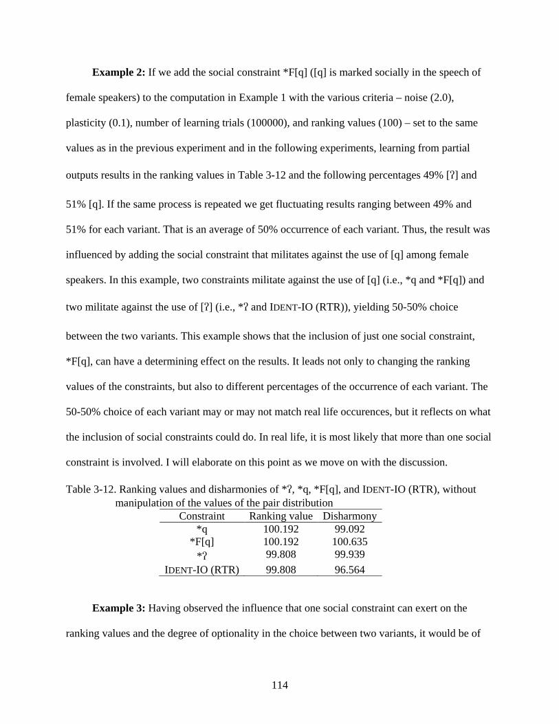
114
Example 2: If we add the social constraint *F[q] ([q] is marked socially in the speech of
female speakers) to the computation in Example 1 with the various criteria – noise (2.0),
plasticity (0.1), number of learning trials (100000), and ranking values (100) – set to the same
values as in the previous experiment and in the following experiments, learning from partial
outputs results in the ranking values in Table 3-12 and the following percentages 49% [] and
51% [q]. If the same process is repeated we get fluctuating results ranging between 49% and
51% for each variant. That is an average of 50% occurrence of each variant. Thus, the result was
influenced by adding the social constraint that militates against the use of [q] among female
speakers. In this example, two constraints militate against the use of [q] (i.e., *q and *F[q]) and
two militate against the use of [] (i.e., * and IDENT-IO (RTR)), yielding 50-50% choice
between the two variants. This example shows that the inclusion of just one social constraint,
*F[q], can have a determining effect on the results. It leads not only to changing the ranking
values of the constraints, but also to different percentages of the occurrence of each variant. The
50-50% choice of each variant may or may not match real life occurences, but it reflects on what
the inclusion of social constraints could do. In real life, it is most likely that more than one social
constraint is involved. I will elaborate on this point as we move on with the discussion.
Table 3-12. Ranking values and disharmonies of *, *q, *F[q], and IDENT-IO (RTR), without manipulation of the values of the pair distribution
Constraint Ranking value Disharmony *q 100.192 99.092
*F[q] 100.192 100.635 * 99.808 99.939
IDENT-IO (RTR) 99.808 96.564
Example 3: Having observed the influence that one social constraint can exert on the
ranking values and the degree of optionality in the choice between two variants, it would be of

115
interest to observe what results would look like if we manipulated the values of the pair
distripution. Conversely, we take the real life percentages of each of [q] and [] in the speech of
female speakers in this study, which are 35% and 65% respectively, and put these percentages as
pair distribution values of [q] and [] respectively in the computation. In this case, learning from
partial outputs in which [] occurs 65% as a result of the *F[q] constraint, and the learner hears
these outputs as inputs, the ranking values of the four constraints in Table 3-12 will be after
100000 learning trials as in Table 3-13. The output distribution will be as follows: 66.5% [] and
33.5% [q], which is very close to the real life percentages. The slight difference in results is
expected because of the learning process and optionality that is held here as a core feature of
variation. Learning from partial outputs that has a higher percentage of [] may result in higher
learning percentage of the [] sound. Thus, our surroundings and the people we interact with may
determine our grammar because they determine the percentage of the input of each of [] and [q].
Further, this alone does not explain why some people may have similar attributes and similar
interactions, yet one switches between the two forms with great success according to the
interlocutor, while one may oscillate between the two forms with the same interlocutor. This is
why I believe that social constraints play a major role in determining our grammars. It depends
on what social constraints are activated at a certain time and place in addition to the input intake.
This will be further examined by the addition of further social constraints to see how results shift
as we add social constraints of various types.
Including the right social constraints and manipulating the pair distribution of [q] and [] to
arrive at the observed variation in the data is important to model the various speakers’ or groups
of speakers’ different grammars. Following this process determines that, for example, the group
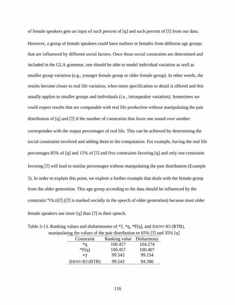
116
of female speakers gets an input of such percent of [q] and such percent of [] from our data.
However, a group of female speakers could have outliers or females from different age groups
that are influenced by different social factors. Once those social constraints are determined and
included in the GLA grammar, one should be able to model individual variation as well as
smaller group variation (e.g., younger female group or older female group). In other words, the
results become closer to real life variation, when more specification or detail is offered and this
usually applies to smaller groups and individuals (i.e., intraspeaker variation). Sometimes we
could expect results that are compatable with real life production without manipulating the pair
distribution of [q] and [] if the number of constraints that favor one sound over another
correspondes with the output percentages of real life. This can be achieved by determining the
social constraints involved and adding them to the computation. For example, having the real life
percentages 85% of [q] and 15% of [] and five constraints favoring [q] and only one constraint
favoring [] will lead to similar percentages without manipulating the pair distribution (Example
5). In order to explain this point, we explore a further example that deals with the female group
from the older generation. This age group according to the data should be influenced by the
constraint *OLD[] ([] is marked socially in the speech of older generation) because most older
female speakers use more [q] than [] in their speech.
Table 3-13. Ranking values and disharmonies of *, *q, *F[q], and IDENT-IO (RTR), manipulating the values of the pair distribution to 65% [] and 35% [q]
Constraint Ranking value Disharmony *q 100.457 104.274
*F[q] 100.457 100.407 * 99.543 99.154
IDENT-IO (RTR) 99.543 94.586
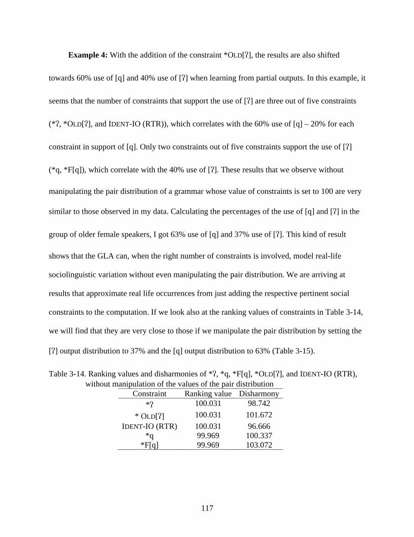
117
Example 4: With the addition of the constraint *OLD[], the results are also shifted
towards 60% use of [q] and 40% use of [] when learning from partial outputs. In this example, it
seems that the number of constraints that support the use of [] are three out of five constraints
(*, *OLD[], and IDENT-IO (RTR)), which correlates with the 60% use of [q] – 20% for each
constraint in support of [q]. Only two constraints out of five constraints support the use of []
(*q, *F[q]), which correlate with the 40% use of []. These results that we observe without
manipulating the pair distribution of a grammar whose value of constraints is set to 100 are very
similar to those observed in my data. Calculating the percentages of the use of [q] and [] in the
group of older female speakers, I got 63% use of [q] and 37% use of []. This kind of result
shows that the GLA can, when the right number of constraints is involved, model real-life
sociolinguistic variation without even manipulating the pair distribution. We are arriving at
results that approximate real life occurrences from just adding the respective pertinent social
constraints to the computation. If we look also at the ranking values of constraints in Table 3-14,
we will find that they are very close to those if we manipulate the pair distribution by setting the
[] output distribution to 37% and the [q] output distribution to 63% (Table 3-15).
Table 3-14. Ranking values and disharmonies of *, *q, *F[q], *OLD[], and IDENT-IO (RTR), without manipulation of the values of the pair distribution
Constraint Ranking value Disharmony * 100.031 98.742
* OLD[] 100.031 101.672 IDENT-IO (RTR) 100.031 96.666
*q 99.969 100.337 *F[q] 99.969 103.072
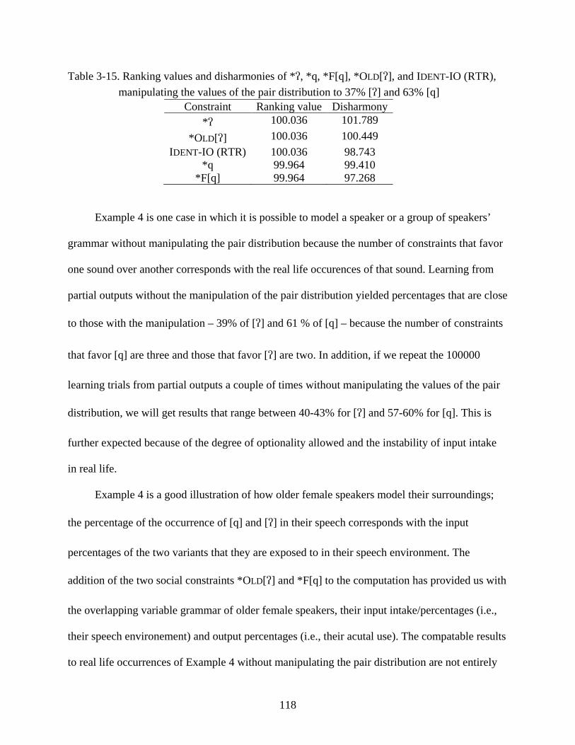
118
Table 3-15. Ranking values and disharmonies of *, *q, *F[q], *OLD[], and IDENT-IO (RTR), manipulating the values of the pair distribution to 37% [] and 63% [q]
Constraint Ranking value Disharmony * 100.036 101.789
*OLD[] 100.036 100.449 IDENT-IO (RTR) 100.036 98.743
*q 99.964 99.410 *F[q] 99.964 97.268
Example 4 is one case in which it is possible to model a speaker or a group of speakers’
grammar without manipulating the pair distribution because the number of constraints that favor
one sound over another corresponds with the real life occurences of that sound. Learning from
partial outputs without the manipulation of the pair distribution yielded percentages that are close
to those with the manipulation – 39% of [] and 61 % of [q] – because the number of constraints
that favor [q] are three and those that favor [] are two. In addition, if we repeat the 100000
learning trials from partial outputs a couple of times without manipulating the values of the pair
distribution, we will get results that range between 40-43% for [] and 57-60% for [q]. This is
further expected because of the degree of optionality allowed and the instability of input intake
in real life.
Example 4 is a good illustration of how older female speakers model their surroundings;
the percentage of the occurrence of [q] and [] in their speech corresponds with the input
percentages of the two variants that they are exposed to in their speech environment. The
addition of the two social constraints *OLD[] and *F[q] to the computation has provided us with
the overlapping variable grammar of older female speakers, their input intake/percentages (i.e.,
their speech environement) and output percentages (i.e., their acutal use). The compatable results
to real life occurrences of Example 4 without manipulating the pair distribution are not entirely
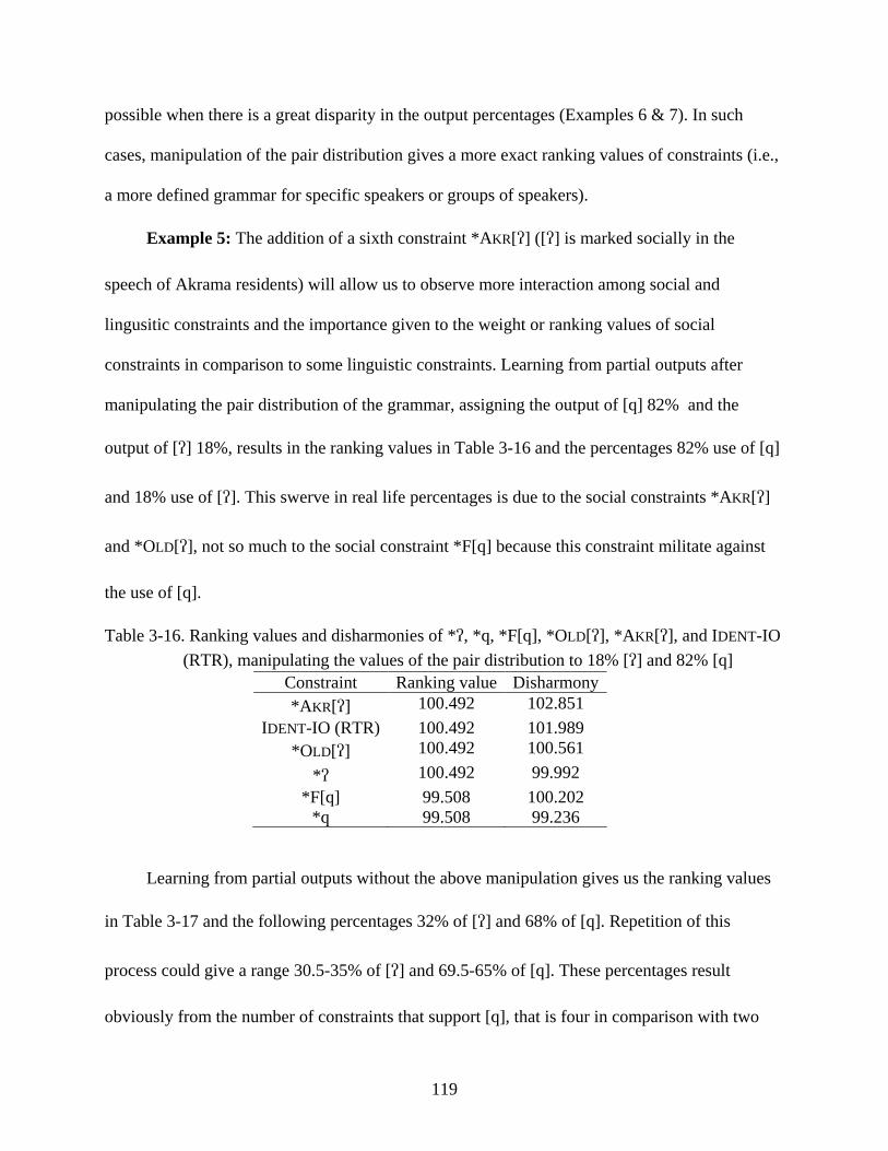
119
possible when there is a great disparity in the output percentages (Examples 6 & 7). In such
cases, manipulation of the pair distribution gives a more exact ranking values of constraints (i.e.,
a more defined grammar for specific speakers or groups of speakers).
Example 5: The addition of a sixth constraint *AKR[] ([] is marked socially in the
speech of Akrama residents) will allow us to observe more interaction among social and
lingusitic constraints and the importance given to the weight or ranking values of social
constraints in comparison to some linguistic constraints. Learning from partial outputs after
manipulating the pair distribution of the grammar, assigning the output of [q] 82% and the
output of [] 18%, results in the ranking values in Table 3-16 and the percentages 82% use of [q]
and 18% use of []. This swerve in real life percentages is due to the social constraints *AKR[]
and *OLD[], not so much to the social constraint *F[q] because this constraint militate against
the use of [q].
Table 3-16. Ranking values and disharmonies of *, *q, *F[q], *OLD[], *AKR[], and IDENT-IO (RTR), manipulating the values of the pair distribution to 18% [] and 82% [q]
Constraint Ranking value Disharmony *AKR[] 100.492 102.851
IDENT-IO (RTR) 100.492 101.989 *OLD[] 100.492 100.561
* 100.492 99.992 *F[q] 99.508 100.202
*q 99.508 99.236
Learning from partial outputs without the above manipulation gives us the ranking values
in Table 3-17 and the following percentages 32% of [] and 68% of [q]. Repetition of this
process could give a range 30.5-35% of [] and 69.5-65% of [q]. These percentages result
obviously from the number of constraints that support [q], that is four in comparison with two
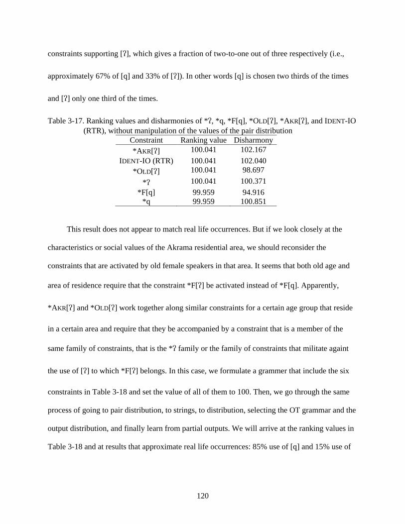
120
constraints supporting [], which gives a fraction of two-to-one out of three respectively (i.e.,
approximately 67% of [q] and 33% of []). In other words [q] is chosen two thirds of the times
and [] only one third of the times.
Table 3-17. Ranking values and disharmonies of *, *q, *F[q], *OLD[], *AKR[], and IDENT-IO (RTR), without manipulation of the values of the pair distribution
Constraint Ranking value Disharmony *AKR[] 100.041 102.167
IDENT-IO (RTR) 100.041 102.040 *OLD[] 100.041 98.697
* 100.041 100.371 *F[q] 99.959 94.916
*q 99.959 100.851
This result does not appear to match real life occurrences. But if we look closely at the
characteristics or social values of the Akrama residential area, we should reconsider the
constraints that are activated by old female speakers in that area. It seems that both old age and
area of residence require that the constraint *F[] be activated instead of *F[q]. Apparently,
*AKR[] and *OLD[] work together along similar constraints for a certain age group that reside
in a certain area and require that they be accompanied by a constraint that is a member of the
same family of constraints, that is the * family or the family of constraints that militate againt
the use of [] to which *F[] belongs. In this case, we formulate a grammer that include the six
constraints in Table 3-18 and set the value of all of them to 100. Then, we go through the same
process of going to pair distribution, to strings, to distribution, selecting the OT grammar and the
output distribution, and finally learn from partial outputs. We will arrive at the ranking values in
Table 3-18 and at results that approximate real life occurrences: 85% use of [q] and 15% use of
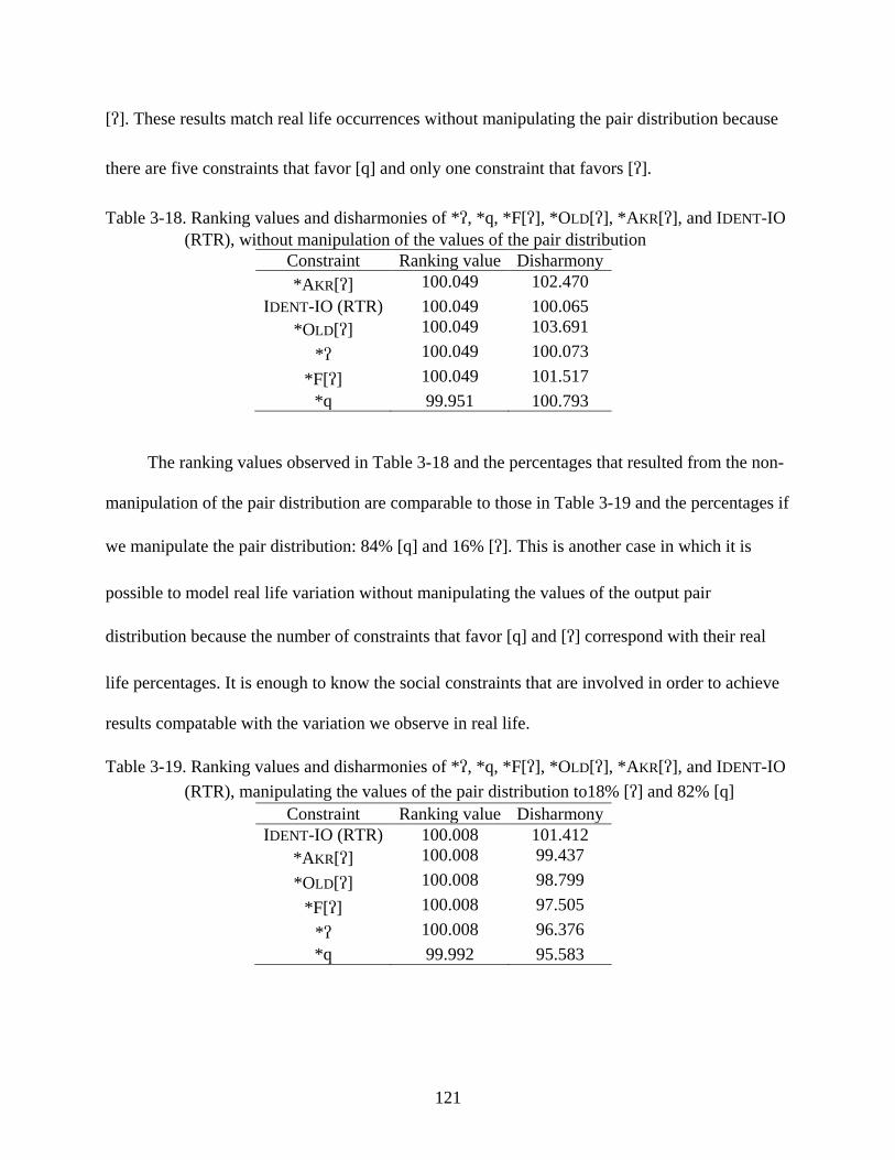
121
[]. These results match real life occurrences without manipulating the pair distribution because
there are five constraints that favor [q] and only one constraint that favors [].
Table 3-18. Ranking values and disharmonies of *, *q, *F[], *OLD[], *AKR[], and IDENT-IO (RTR), without manipulation of the values of the pair distribution
Constraint Ranking value Disharmony *AKR[] 100.049 102.470
IDENT-IO (RTR) 100.049 100.065 *OLD[] 100.049 103.691
* 100.049 100.073 *F[] 100.049 101.517
*q 99.951 100.793
The ranking values observed in Table 3-18 and the percentages that resulted from the non-
manipulation of the pair distribution are comparable to those in Table 3-19 and the percentages if
we manipulate the pair distribution: 84% [q] and 16% []. This is another case in which it is
possible to model real life variation without manipulating the values of the output pair
distribution because the number of constraints that favor [q] and [] correspond with their real
life percentages. It is enough to know the social constraints that are involved in order to achieve
results compatable with the variation we observe in real life.
Table 3-19. Ranking values and disharmonies of *, *q, *F[], *OLD[], *AKR[], and IDENT-IO (RTR), manipulating the values of the pair distribution to18% [] and 82% [q]
Constraint Ranking value Disharmony IDENT-IO (RTR) 100.008 101.412
*AKR[] 100.008 99.437 *OLD[] 100.008 98.799
*F[] 100.008 97.505 * 100.008 96.376 *q 99.992 95.583
122
Thus, like SG, the GLA can easily model sociolinguistic variation. It can give us
probabilities of variation that could reflect real life variation based on incorporating the right
type and number of social constraints. However, it exceeds SG in that it is capable of modeling
any speaker’s or group’s variable grammar through manipulation of the output pair distribution.
The GLA dispenses with trying all possible rankings of constraints to arrive at the frequencies of
each variant. Even all possible rankings of constraints may not reflect the exact real life
percentages of variants and do not provide explanation of why such inter- and intra-speaker
sociolinguistic variation exists. I have also argued that the inclusion of social constraints in the
GLA, in addition to the manipulation of pair distribution, is essential to explain linguistic
differences among speakers from the same social group or different social groups and to model
sociolinguistic variation in formal theory. In addition, certain social constraints could give us
expectations about what other speakers’ speech should sound like. In Example 5, the
constraints*F[], *OLD[], and *AKR[] make us expect limited use of [] in the speech of older
female speakers from Akrama. What is expected from these constraints is what we observe in the
speech of older female speakers from Akrama in real life. In this sense, listeners may also be
able to discover the grammar used by a certain speaker or group of speakers and the social
constraints activated by those speakers at a certain time and place, as some interviewees’
comments indicate. That is, they observe variation in the speech of their relatives based on the
interlocutor. These interviewees point out their awareness of such shift in pronunciation, when it
takes place, and with whom it takes place. This awareness may be an indication of their
knowledge of the various social constraints and various grammars that exist in their community
and that result from different activations of different social constraints. In support of this
argument, I will explore one further example.
123
Example 6: Similarly, if we only replace *F[] with the constraint *M[] ([] is marked
socially in the speech of male speakers) and learn from partial outputs, the percentages of each of
[q] and [] will be after 100000 learning trials: 84% and 16% respectively. These percentages are
also close to real life occurences. In our case, [q] occurs 96% in the speech of older male
speakers from Akrama. This precentage may be lower and closer to 84% if the sample is taken
from more than three speakers, which is the number of older male speakers from Akrama that are
part of my original data. It seems that the following social constraints *AKR[], *M[] and
*OLD[] play a major role in determining the results and the precentages of each of [] and [q].
They make us expect a low percentage of [] and this is the case in older male speakers from
Akrama. Since the percentage of [] in older male speakers from Akrama is lower than that of
older female speakers from Akrama and the only constraint that differs between the two social
groups is *M[] instead of *F[], we can conclude that *M[] gives lower percentages of [] in
the speech of male speakers than does *F[] in the speech of female speakers. In other words,
*M[] has a higher ranking value than *F[] in all speakers. It makes speakers and listeners
expect a difference between the speech of males and females (i.e., less [] and more [q] in the
speech of males than in the speech of females).
If we change the percentages of the pair distibution we get from the OT grammar that
include the six constraints in Table 3-20 and that resulted in 16% [] and 84% [q] to 96% [q] and
4% [], we will get from learning from partial outputs the ranking values in Table 3-20 and the
approximate percentages: 94% use of [q] and 6% use of []. Table 3-20 shows that *M[] has a
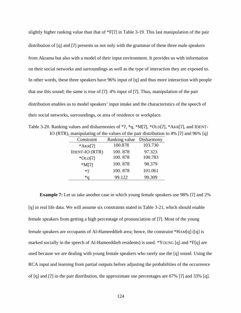
124
slightly higher ranking value than that of *F[] in Table 3-19. This last manipulation of the pair
distribution of [q] and [] presents us not only with the grammar of these three male speakers
from Akrama but also with a model of their input environment. It provides us with information
on their social networks and surroundings as well as the type of interaction they are exposed to.
In other words, these three speakers have 96% input of [q] and thus more interaction with people
that use this sound; the same is true of []: 4% input of []. Thus, manipulation of the pair
distribution enables us to model speakers’ input intake and the characteristics of the speech of
their social networks, surroundings, or area of residence or workplace.
Table 3-20. Ranking values and disharmonies of *, *q, *M[], *OLD[], *AKR[], and IDENT-IO (RTR), manipulating of the values of the pair distribution to 4% [] and 96% [q]
Constraint Ranking value Disharmony *AKR[] 100.878 103.730
IDENT-IO (RTR) 100. 878 97.323 *OLD[] 100. 878 100.783 *M[] 100. 878 98.379
* 100. 878 101.061 *q 99.122 99.309
Example 7: Let us take another case in which young female speakers use 98% [] and 2%
[q] in real life data. We will assume six constraints stated in Table 3-21, which should enable
female speakers from getting a high percentage of pronunciation of []. Most of the young
female speakers are occupants of Al-Hameeddieh area; hence, the constraint *HAM[q] ([q] is
marked socially in the speech of Al-Hameeddieh residents) is used. *YOUNG [q] and *F[q] are
used because we are dealing with young female speakers who rarely use the [q] sound. Using the
RCA input and learning from partial outputs before adjusting the probabilities of the occurrence
of [q] and [] in the pair distribution, the approximate use percentages are 67% [] and 33% [q].
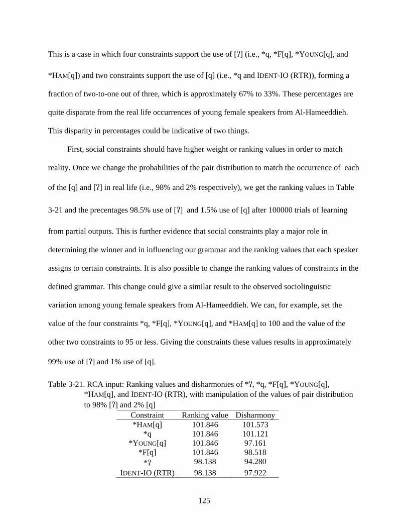
125
This is a case in which four constraints support the use of [] (i.e., *q, *F[q], *YOUNG[q], and
*HAM[q]) and two constraints support the use of [q] (i.e., *q and IDENT-IO (RTR)), forming a
fraction of two-to-one out of three, which is approximately 67% to 33%. These percentages are
quite disparate from the real life occurrences of young female speakers from Al-Hameeddieh.
This disparity in percentages could be indicative of two things.
First, social constraints should have higher weight or ranking values in order to match
reality. Once we change the probabilities of the pair distribution to match the occurrence of each
of the [q] and [] in real life (i.e., 98% and 2% respectively), we get the ranking values in Table
3-21 and the precentages 98.5% use of [] and 1.5% use of [q] after 100000 trials of learning
from partial outputs. This is further evidence that social constraints play a major role in
determining the winner and in influencing our grammar and the ranking values that each speaker
assigns to certain constraints. It is also possible to change the ranking values of constraints in the
defined grammar. This change could give a similar result to the observed sociolinguistic
variation among young female speakers from Al-Hameeddieh. We can, for example, set the
value of the four constraints *q, *F[q], *YOUNG[q], and *HAM[q] to 100 and the value of the
other two constraints to 95 or less. Giving the constraints these values results in approximately
99% use of [] and 1% use of [q].
Table 3-21. RCA input: Ranking values and disharmonies of *, *q, *F[q], *YOUNG[q], *HAM[q], and IDENT-IO (RTR), with manipulation of the values of pair distribution to 98% [] and 2% [q]
Constraint Ranking value Disharmony *HAM[q] 101.846 101.573
*q 101.846 101.121 *YOUNG[q] 101.846 97.161
*F[q] 101.846 98.518 * 98.138 94.280
IDENT-IO (RTR) 98.138 97.922
126
Second, the input of the younger generation is the HCA form, not the RCA form.
Changing the input to // instead of /q/ in the above computation yields without manipulation of
the pair distribution of [] and [q] the approximate percentages 83% use of [] and 17% use of
[q]. These percentages are the result of five constraints in support of the use of [] (i.e., *q,
*F[q], *YOUNG[q], *HAM[q], and IDENT-IO (RTR)) and only one constraint in support of the use
of [q], that is *. Changing the young generation’s input from /q/ to // without manipulating the
pair distribution gives percentages that are closer to those of the real life occurrences of [q] and
[] in the speech of young female speakers, although the resulting percentages are not the exact
percentages of those speakers. In the initial stage of Example 7, we got the percentages 67% use
of [] and 33% use of [q] when the input was the RCA form, which are very different from the
real life occurrences of [q] and [] in the speech of young female speakers from Al-Hameeddieh.
This raises issue of the ability of the younger generation to restructure their input. I believe that
not only do social constraints exert an effect on the younger generation’s grammar but also that
the younger generation has succeeded in restructuring their input. Their input becomes the HCA
input instead of the RCA input. Conversely, the input should contain // instead of /q/. Being
born in the city of Hims, although to a rural family that uses the overt form [q] at home, and
being exposed from an early age to the overt form [] at school, the younger generation may
have been able to restructure their parents’ input from listening to the majority of their
environment’s input (i.e., friends at school). This means the younger generation, perhaps, do not
have /q/ in their phonemic inventory any more; all they have is // like HCA speakers and they
tend to neutralize in the same way.
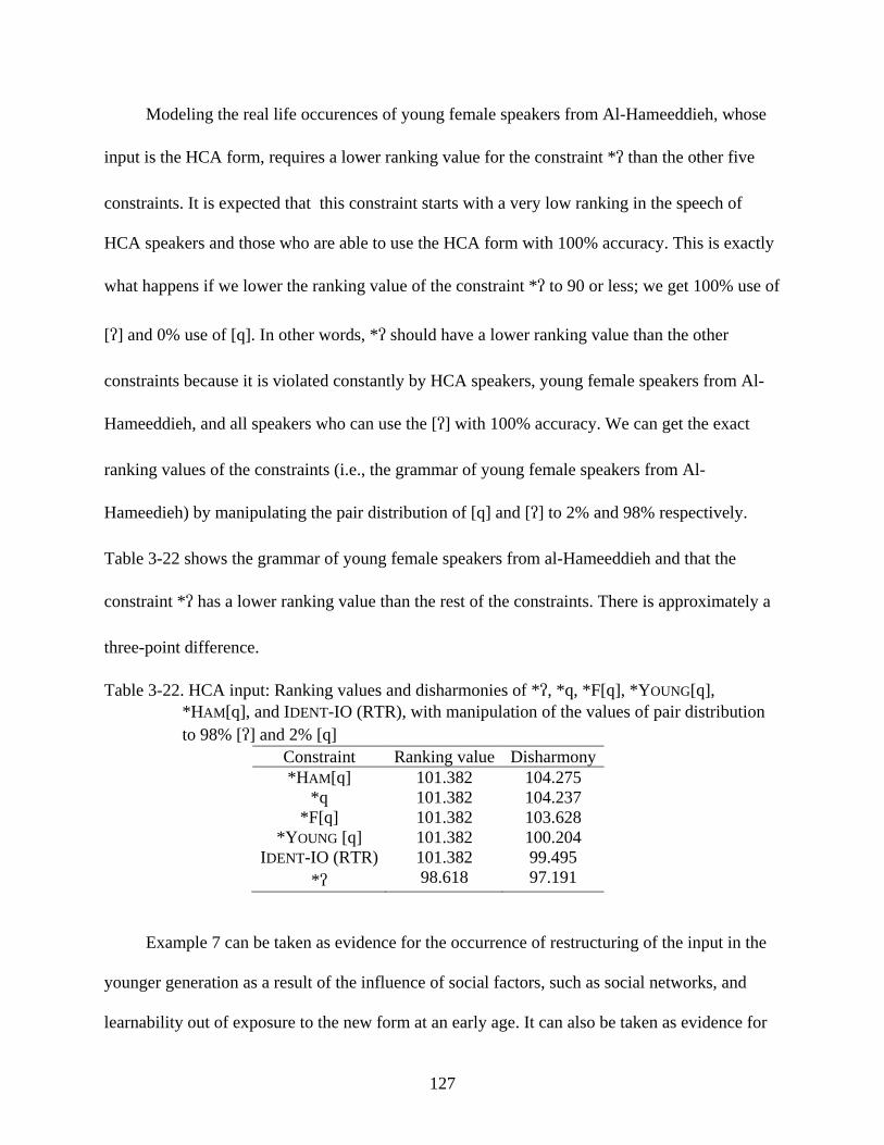
127
Modeling the real life occurences of young female speakers from Al-Hameeddieh, whose
input is the HCA form, requires a lower ranking value for the constraint * than the other five
constraints. It is expected that this constraint starts with a very low ranking in the speech of
HCA speakers and those who are able to use the HCA form with 100% accuracy. This is exactly
what happens if we lower the ranking value of the constraint * to 90 or less; we get 100% use of
[] and 0% use of [q]. In other words, * should have a lower ranking value than the other
constraints because it is violated constantly by HCA speakers, young female speakers from Al-
Hameeddieh, and all speakers who can use the [] with 100% accuracy. We can get the exact
ranking values of the constraints (i.e., the grammar of young female speakers from Al-
Hameedieh) by manipulating the pair distribution of [q] and [] to 2% and 98% respectively.
Table 3-22 shows the grammar of young female speakers from al-Hameeddieh and that the
constraint * has a lower ranking value than the rest of the constraints. There is approximately a
three-point difference.
Table 3-22. HCA input: Ranking values and disharmonies of *, *q, *F[q], *YOUNG[q], *HAM[q], and IDENT-IO (RTR), with manipulation of the values of pair distribution to 98% [] and 2% [q]
Constraint Ranking value Disharmony *HAM[q] 101.382 104.275
*q 101.382 104.237 *F[q] 101.382 103.628
*YOUNG [q] 101.382 100.204 IDENT-IO (RTR) 101.382 99.495
* 98.618 97.191
Example 7 can be taken as evidence for the occurrence of restructuring of the input in the
younger generation as a result of the influence of social factors, such as social networks, and
learnability out of exposure to the new form at an early age. It can also be taken as evidence for
128
the dormancy of some linguistic constraints, such as *, in some speakers and the activation of
other constraints instead. The example further shows the importance of social constraints in
comparison to some linguistics constraints in determing a speaker’s grammar. It is worth noting
here that even in cases where the percentages are a little different from real life data, these
examples show that social constraints do influence our selection of a ranking value for a certain
linguistic constraint and do play a role in our choice of a grammar at a certain time or place.
These social constraints determine the approximate number of times each output occurs (i.e., the
percentage of the occurrence of each variant).
3.2.4 Concluding Remarks on the Sociolinguistic Variation between [q] and []
The above examples have shown that the manipulation of the pair distribution can model
the different grammars of different speakers or groups of speakers. To explain the differences
among those speakers or groups of speakers, it was essential to include social constraints in the
computation. Manipulating the pair distribution of the linguistic constraints alone does not
explain why speakers’ speech differs from each other in a sociolinguistic variation situation or
why speakers from the same social group or different social groups have different grammars.
Furthermore, the above examples have shown that certain social constraints may give us
expectations about what a speaker’s or a group of speakers’ speech should sound like. For
example, the bundling of the constraints *F[], *Old[], and *AKR[] in Example 5 tells us to
expect very low percentage of [] in the speech of older female speakers from Akrama but a little
higher than the percentage of [] in the speech of older male speakers from Akrama. As a result,
the [] sound is probably more marked among older male speakers from Akrama, leading to the
suggestion that the constraint *M[] is probably ranked higher than *F[] and is assigned a
129
higher ranking value by male and female speakers alike. Ranking constraints that are activated
by other speakers highlight the importance of the inclusion of social constraints in the
computation in the case of a sociolinguistic variation. Having the constraint *M[] ranked higher
than other constraints in the grammar of all speakers means that the listener should expect what
the interlocutor’s speech should sound like based on whether the interlocutor is a rural male or
female migrant speaker to the city13. In the same way that an RCA speaker expects an HCA
speaker to produce [] as a result of a different grammar, an RCA speaker may expect what an
older male migrant speaker should sound like and simultaneously the social constraints that
allow him to speak in a certain way or to make choices of his grammar. A listener who listens to
a speaker in two different setting using a different form in each of the settings is aware of that
speaker’s change of grammar and is most likely aware of the social contraints involved in that
switch according to the interlocutor.
In addition, the above examples present how each speaker or group of speakers can model
their environment. Examples 4, 5 and 7 show that female speakers model their environment and
so do male speakers in Example 6. It also seems from Examples 5 and 6 that female speakers are
capable of modeling their environment, the HCA setting, better than male speaker. Thus, it may
be possible to predict that males use the [q] sound more than females because of their activation
13 This does not exclude the possibility that males may be exposed more to the [q] sound than females are. In other words, they associate more with people (particularly males) from their own background and maintain their [q] sound to express solidarity. Such associations with people who use their own native sound expose males to higher output (i.e., input for the learner) percentages of the [q] sound (i.e., the pair distribution from which they learn is inclined more towards the [q] sound than it is in females). Learning from higher percentages of [q] leads to higher production percentages of [q] because the surrounding linguistic environment of speakers influences their degree of learnability of a form. In other words, males do not learn the new form, [], as much as females do because they are not as exposed to it as females are. Their production (i.e., learnability) is affected by the pair distribution of [q] and [] in their environment. Even in the case of different pair distribution of [q] and [] for males and females, *M[] will have in the computation a slightly higher ranking value than *F[] to match this difference (Compare Table 3-20 to Table 3-19).
130
of the *M[] constraint that is as aforementioned more fatal or has higher ranking among gender
constraints than *F[]. Thus, social constraints within one social factor may have a variety of
strength and ranking values based on the social significance or markedness of a sound to a
particular gender, age group, residential area, social class, etc. In my data, *M[] may be more
fatal than *F[], but in other social settings or linguistic environment, *F[] may be more fatal
because [] is considered more marked among females than among males. This does not only
apply to the constraints proposed in this study, but could apply to other social constraints that are
pertinent to other varieties or languages. All what has been mentioned so far support the
psychological reality of the model and the constraints involved in the computation, particularly
when we speak of choice, expectations, and awareness of one’s grammar as well as the other’s
grammar.
3.3 Modeling Variation between [t] and [s] and between [d] and [z]
After discussing the variable use of [q] and [] and their modeling in the GLA by
proposing social constraints and incorporating them in the computation process, I move our
attention to the variable use of [t] and [s] and [d] and [z] in the colloquial speech of HCA and
RCA speakers. I refer to this type of variation as stable because each variant occurs in particular
words of the RCA and HCA dialects; there is no interchangeability between the variants. This
type of variation is different from the variation observed between [q] and []. The latter can be
considered of the gradient type because it varies based on a number of social factors. The former
is more of the categorical type because it does not vary within a speaker, among speakers, or
among groups of speakers. The same variant is used by all speakers to pronounce certain words
131
(Chapter 5). In this sense, it could be referred to as a phenomenon in its current state rather than
variation. This current stable phenomenon may have resulted from variation historically.
The first two variants, [t] and [s], are pronounced [] in SA and the latter two variants, [d]
and [z] are pronounced []. In other words, the SA variants do not exist anymore in HCA or
RCA speech except in very rare use of lexical borrowings from SA that contain those two
variants. The SA variants [] and [] merged completely with [t] and [d] respectively around the
14th century (Daher, 1998a, 1999). This was the first historical change in the history of the SA
variants [] and [] (Schmidt 1974: 94, cited in Daher 1999, 164). The second change took place
some time after the 14th century (Birkeland 1952; Schmidt 1986: 57; Schulz 1981:33; all cited in
Daher 1999); some [] and [] variants in borrowed words from SA were replaced in colloquial
speech with [s] and [z] respectively. According to Daher (1999), the sounds [] and [] might
only appear in the speech of some Damascene speakers who are highly educated and whose jobs
involve extensive use of the written language, SA. Daher tries to argue that the appearance of the
SA variants [] and [] in colloquial speech as [s] and [z] respectively is due to attempting to
imitate the SA variants but pronouncing them as [s] amd [z] instead (p. 164). According to
Daher, the use of [s] and [z] is more elevated than the use of [t] and [d] respectively, despite
being also dialectal variants. Thus, some speakers may produce [s] and [z] when aiming at
producing the SA variants [] and [] respectively. However, he discovered that the observed
variation between [t] and [s] and between [d] and [z] is “stable” (p. 180) with no indication of
any change in progress. Daher dealt with the variants of interest from a different perspective; he
treated them as ternary and binary variables. The ternary variables are [t] and [d] and the binary
variables are [s] and [z]. Ternary refers to the possibility of using the three forms in one word
132
interchangeably. For example, [t], [s], or [] can occur in the word for ‘snow’: [tal], [sal], or
[al]. In this case, the underlying forms for all the variants would be /t/. It would be /d/ for
words that can be pronounced with either [d], [z], or []. On the other hand, the underlying form
for binary variables would be /s/ and /z/ because words can be pronounced with either [s] and []
or [z] and []. Daher’s findings are different from the findings in this study because his primary
purpose was comparing females’ and males’ use of standard and colloquial variants. These
findings are based on his data that were probably elicited in a less natural way, in that people
used the [] or the [s] sounds instead of [t] and the [] and [z] sounds instead of [d] in words that
are normally pronounced in colloquial speech with [t] and [d] respectively. According to Daher
(1998: 2), the sociolinguistic interview could elicit spoken SA from educated speakers outside a
formal setting, such as television and radio broadcasting, public speeches, journalism, etc. This is
not the case in my data. All speakers spoke naturally using their dialectal variants all the time.
They used specifically [t] in some words and specifically [s] in other words in place of the SA
variant []. The same applies for the use of [d] and [z]; each is used specifically in certain words
instead of the SA variant []. For this reason, I call this kind of variation stable variation, and I
suggest that each variant has its own underlying form that is the surface form of each one of
them, which is found in the colloquial speech of RCA and HCA speakers. In this sense, /t/ is the
underlying form for [t]; /s/ for [s]; /d/ for [d]; and /z/ for [z]. I will also argue that the two SA
phonemes // and // are absent from the inventory of RCA and HCA speakers (Appendix F).
The difference between HCA and RCA, on the one hand, and SA, on the other hand, is
illustrated in Table 3-23.
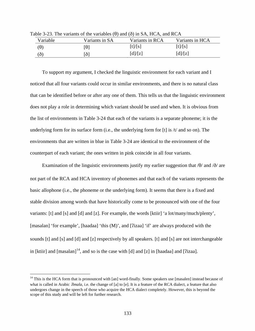
133
Table 3-23. The variants of the variables () and () in SA, HCA, and RCA Variable Variants in SA Variants in RCA Variants in HCA () [] [t]/[s] [t]/[s] () [] [d]/[z] [d]/[z]
To support my argument, I checked the linguistic environment for each variant and I
noticed that all four variants could occur in similar environments, and there is no natural class
that can be identified before or after any one of them. This tells us that the linguistic environment
does not play a role in determining which variant should be used and when. It is obvious from
the list of environments in Table 3-24 that each of the variants is a separate phoneme; it is the
underlying form for its surface form (i.e., the underlying form for [t] is /t/ and so on). The
environments that are written in blue in Table 3-24 are identical to the environment of the
counterpart of each variant; the ones written in pink coincide in all four variants.
Examination of the linguistic environments justify my earlier suggestion that // and // are
not part of the RCA and HCA inventory of phonemes and that each of the variants represents the
basic allophone (i.e., the phoneme or the underlying form). It seems that there is a fixed and
stable division among words that have historically come to be pronounced with one of the four
variants: [t] and [s] and [d] and [z]. For example, the words [ktiir] ‘a lot/many/much/plenty’,
[masalan] ‘for example’, [haadaa] ‘this (M)’, and [izaa] ‘if’ are always produced with the
sounds [t] and [s] and [d] and [z] respectively by all speakers. [t] and [s] are not interchangeable
in [ktiir] and [masalan]14, and so is the case with [d] and [z] in [haadaa] and [izaa].
14 This is the HCA form that is pronounced with [an] word-finally. Some speakers use [masalen] instead because of what is called in Arabic imala, i.e. the change of [a] to [e]. It is a feature of the RCA dialect, a feature that also undergoes change in the speech of those who acquire the HCA dialect completely. However, this is beyond the scope of this study and will be left for further research.
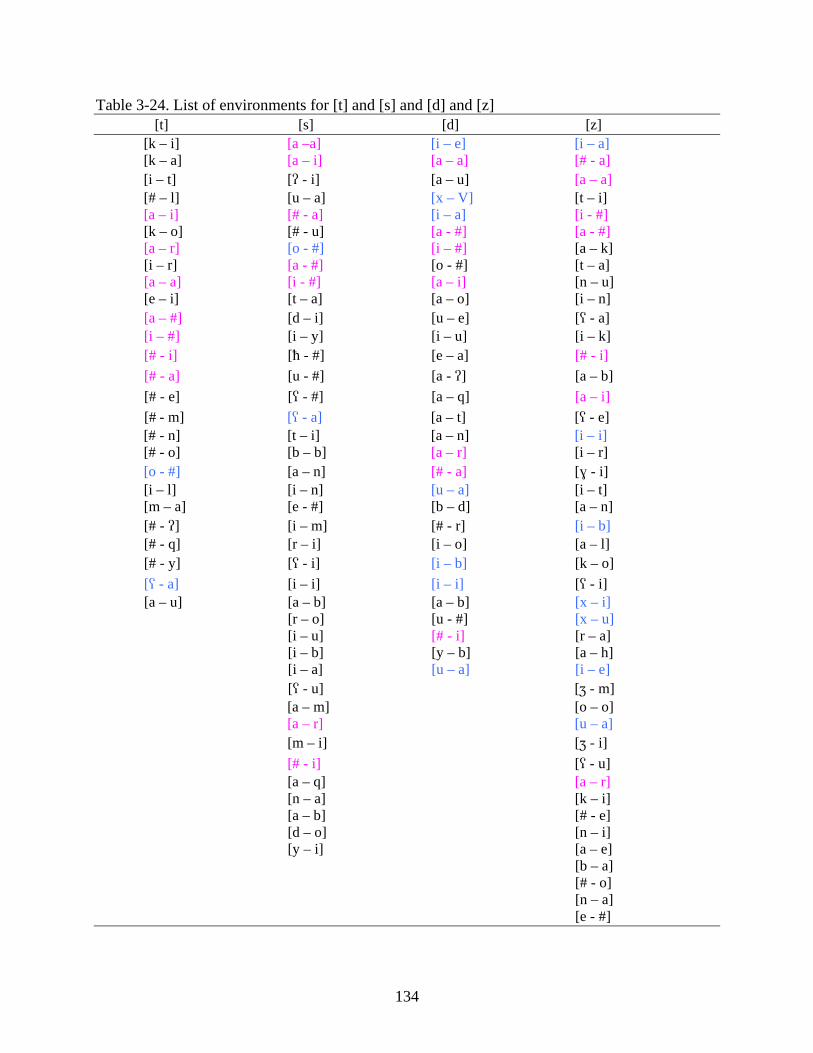
134
Table 3-24. List of environments for [t] and [s] and [d] and [z] [t] [s] [d] [z]
[k – i] [a –a] [i – e] [i – a] [k – a] [a – i] [a – a] [# - a] [i – t] [ - i] [a – u] [a – a] [# – l] [u – a] [x – V] [t – i] [a – i] [# - a] [i – a] [i - #] [k – o] [# - u] [a - #] [a - #] [a – r] [o - #] [i – #] [a – k] [i – r] [a - #] [o - #] [t – a] [a – a] [i - #] [a – i] [n – u] [e – i] [t – a] [a – o] [i – n] [a – #] [d – i] [u – e] [ - a] [i – #] [i – y] [i – u] [i – k] [# - i] [ - #] [e – a] [# - i] [# - a] [u - #] [a - ] [a – b] [# - e] [ - #] [a – q] [a – i] [# - m] [ - a] [a – t] [ - e] [# - n] [t – i] [a – n] [i – i] [# - o] [b – b] [a – r] [i – r] [o - #] [a – n] [# - a] [ - i] [i – l] [i – n] [u – a] [i – t] [m – a] [e - #] [b – d] [a – n] [# - ] [i – m] [# - r] [i – b] [# - q] [r – i] [i – o] [a – l] [# - y] [ - i] [i – b] [k – o] [ - a] [i – i] [i – i] [ - i] [a – u] [a – b] [a – b] [x – i]
[r – o] [u - #] [x – u] [i – u] [# - i] [r – a] [i – b] [y – b] [a – h] [i – a] [u – a] [i – e] [ - u] [ - m] [a – m] [o – o] [a – r] [u – a] [m – i] [ - i] [# - i] [ - u] [a – q] [a – r] [n – a] [k – i] [a – b] [# - e] [d – o] [n – i] [y – i] [a – e] [b – a] [# - o] [n – a] [e - #]
135
3.3.1 Linguistic Constraints Pertinent to the Variation between [t] and [s] and [d] and [z]
Because of the fixed and stable variation that is observed in the data, I propose a number of
linguistic constraints that are required for the maintenance of the four variants in their respective
words. Since the SA variants [] and [] are not observed in the data, I assume that they are not
part of the phonemic system of speakers. In other words, the SA variables // and // are absent
from the speakers’ phonemic inventory. The context-free markedness constraints militating
against these two sounds (i.e., * and *) will be undominated in the grammar of speakers’
speech. What is present in speakers’ phonemic repertoire are the observed variants in the data:
/t/, /s/, /d/, and /z/. For example, the SA words /alaaa/ ‘three’ and /haaaa/ ‘this (M)’ are
always pronounced in RCA and HCA as [tlaati] and [haadaa] respectively. Since this applies to
all speakers, there is no reason to believe there is an underlying form that is different from the
surface form. The existence of all four variants (/t/, /s/, /d/, and /z/) in the speech of speakers
impels us to suggest four context-free markedness constraints that militate against each of the
four variants in attempt to eliminate it from or prevent it from occurring in certain words. These
four context-free markedness constraints are:
(12) *t Voiceless alveolar stop is marked (13) *s Voiceless alveolar fricative is marked (14) *d Voiced alveolar stop is marked (15) *z Voiced alveolar fricative is marked
A switch from the use of [t] to the use of [s], for example, or vice versa involves a manner
of articulation change: a change from a stop to a fricative or from a fricative to a stop, and so is
the case with respect to switching between [d] and [z]. Hence, we need the following faithfulness
constraints to maintain the friction and stop features in the input:

136
(16) IDENT-IO (Fric) Let α be a segment in the input, and β a correspondent of α in the output. If α is [γFric], then β is [γFric]
(17) IDENT-IO (Stop) Let α be a segment in the input, and β a correspondent of α
in the output. If α is [γStop], then β is [γStop] Any change from /t/ into [s], /s/ into [t], /d/ into [z], and /z/ into [d] will result in violation of one
of the two constraints in (16) and (17). Since both constraints in (16) and (17) militate against the
change of some manner of articulation, we can combine them in one IDENT-IO constraint for
manner:
(18) IDENT-IO (Manner) Let α be a segment in the input, and β a correspondent of α in the output. If α is [γManner], then β is [γManner]
The constraint in (18) is sufficient to prevent any change in the manner of articulation and
guarantees that all input forms will have equivalent corresponding output forms. In other words,
the faithfulness constraint must be higher ranked than the four markedness constraints to
preserve the input in the output. The ranking among the four markedness constraints is irrelevant
because they are all violable since all fours sounds are possible in natural speech.
3.3.2 Faithfulness and the Variants [t] and [s] and [d] and [z]
Here, I will follow the same process that I followed in modeling the variable use of [q] and
[]. I define a number of grammars. The ranking value of constraints will be set at 100 unless
specified otherwise. Each grammar will be forwarded to pair distribution, then to strings and to
distributions. We learn from partial outputs by selecting the output string or the output
distribution with the defined OT grammar. The number of learning trials is 100,000 unless
specified otherwise with 0.2 noise and 0.1 plasticity. The underlying form is assumed to be the
surface form of the speakers, that is /ktiir/ for [ktiir] and /masalan/ for [masalan], for example. I
will start examining the variable use of [t] and [s], using the two mentioned underlying forms as
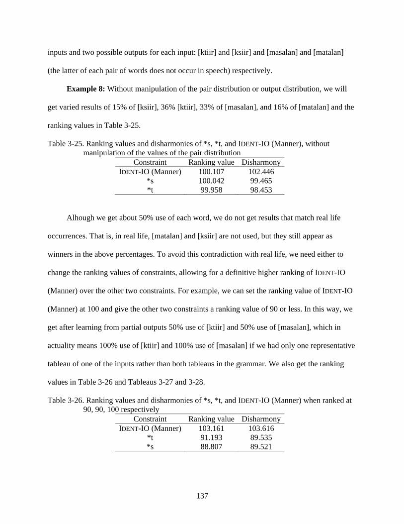
137
inputs and two possible outputs for each input: [ktiir] and [ksiir] and [masalan] and [matalan]
(the latter of each pair of words does not occur in speech) respectively.
Example 8: Without manipulation of the pair distribution or output distribution, we will
get varied results of 15% of [ksiir], 36% [ktiir], 33% of [masalan], and 16% of [matalan] and the
ranking values in Table 3-25.
Table 3-25. Ranking values and disharmonies of *s, *t, and IDENT-IO (Manner), without manipulation of the values of the pair distribution
Constraint Ranking value Disharmony IDENT-IO (Manner) 100.107 102.446
*s 100.042 99.465 *t 99.958 98.453
Alhough we get about 50% use of each word, we do not get results that match real life
occurrences. That is, in real life, [matalan] and [ksiir] are not used, but they still appear as
winners in the above percentages. To avoid this contradiction with real life, we need either to
change the ranking values of constraints, allowing for a definitive higher ranking of IDENT-IO
(Manner) over the other two constraints. For example, we can set the ranking value of IDENT-IO
(Manner) at 100 and give the other two constraints a ranking value of 90 or less. In this way, we
get after learning from partial outputs 50% use of [ktiir] and 50% use of [masalan], which in
actuality means 100% use of [ktiir] and 100% use of [masalan] if we had only one representative
tableau of one of the inputs rather than both tableaus in the grammar. We also get the ranking
values in Table 3-26 and Tableaus 3-27 and 3-28.
Table 3-26. Ranking values and disharmonies of *s, *t, and IDENT-IO (Manner) when ranked at 90, 90, 100 respectively
Constraint Ranking value Disharmony IDENT-IO (Manner) 103.161 103.616
*t 91.193 89.535 *s 88.807 89.521
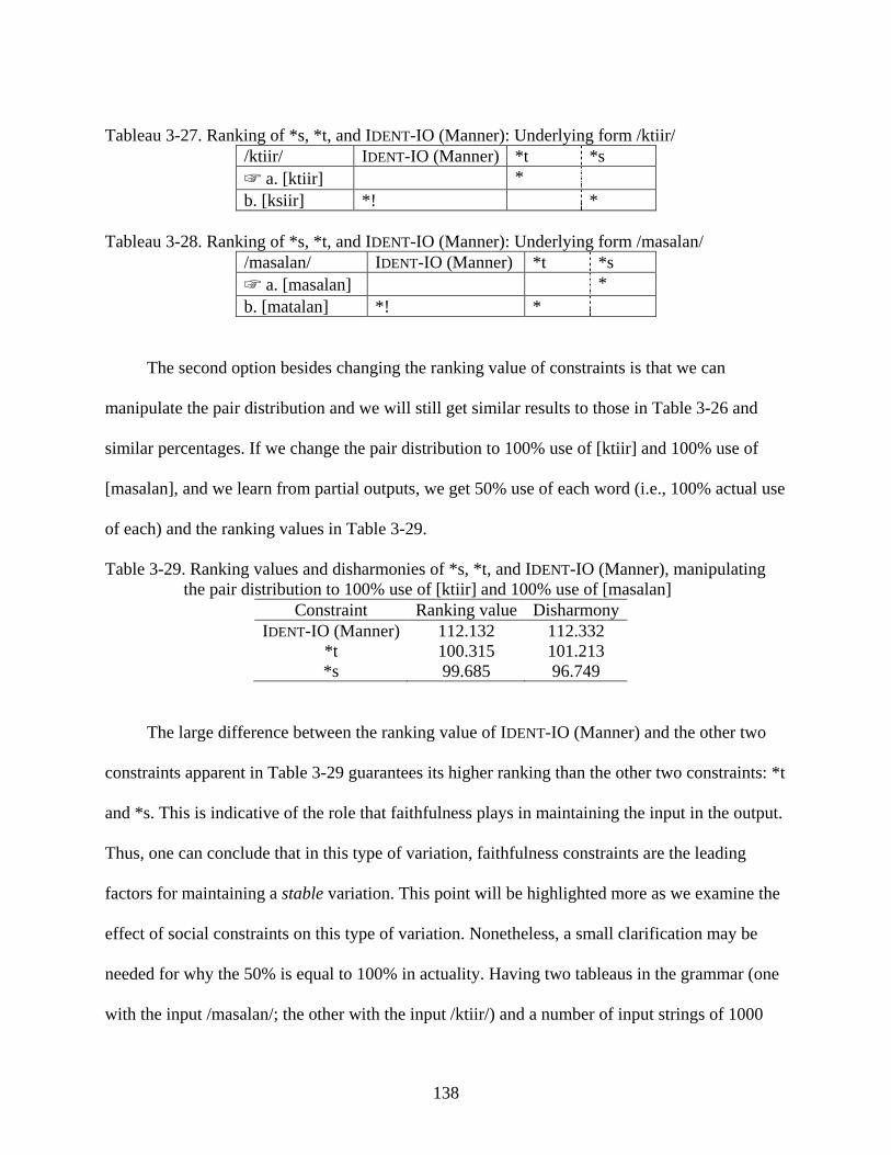
138
Tableau 3-27. Ranking of *s, *t, and IDENT-IO (Manner): Underlying form /ktiir/
/ktiir/ IDENT-IO (Manner) *t *s ☞ a. [ktiir] * b. [ksiir] *! *
Tableau 3-28. Ranking of *s, *t, and IDENT-IO (Manner): Underlying form /masalan/
/masalan/ IDENT-IO (Manner) *t *s ☞ a. [masalan] * b. [matalan] *! *
The second option besides changing the ranking value of constraints is that we can
manipulate the pair distribution and we will still get similar results to those in Table 3-26 and
similar percentages. If we change the pair distribution to 100% use of [ktiir] and 100% use of
[masalan], and we learn from partial outputs, we get 50% use of each word (i.e., 100% actual use
of each) and the ranking values in Table 3-29.
Table 3-29. Ranking values and disharmonies of *s, *t, and IDENT-IO (Manner), manipulating the pair distribution to 100% use of [ktiir] and 100% use of [masalan]
Constraint Ranking value Disharmony IDENT-IO (Manner) 112.132 112.332
*t 100.315 101.213 *s 99.685 96.749
The large difference between the ranking value of IDENT-IO (Manner) and the other two
constraints apparent in Table 3-29 guarantees its higher ranking than the other two constraints: *t
and *s. This is indicative of the role that faithfulness plays in maintaining the input in the output.
Thus, one can conclude that in this type of variation, faithfulness constraints are the leading
factors for maintaining a stable variation. This point will be highlighted more as we examine the
effect of social constraints on this type of variation. Nonetheless, a small clarification may be
needed for why the 50% is equal to 100% in actuality. Having two tableaus in the grammar (one
with the input /masalan/; the other with the input /ktiir/) and a number of input strings of 1000
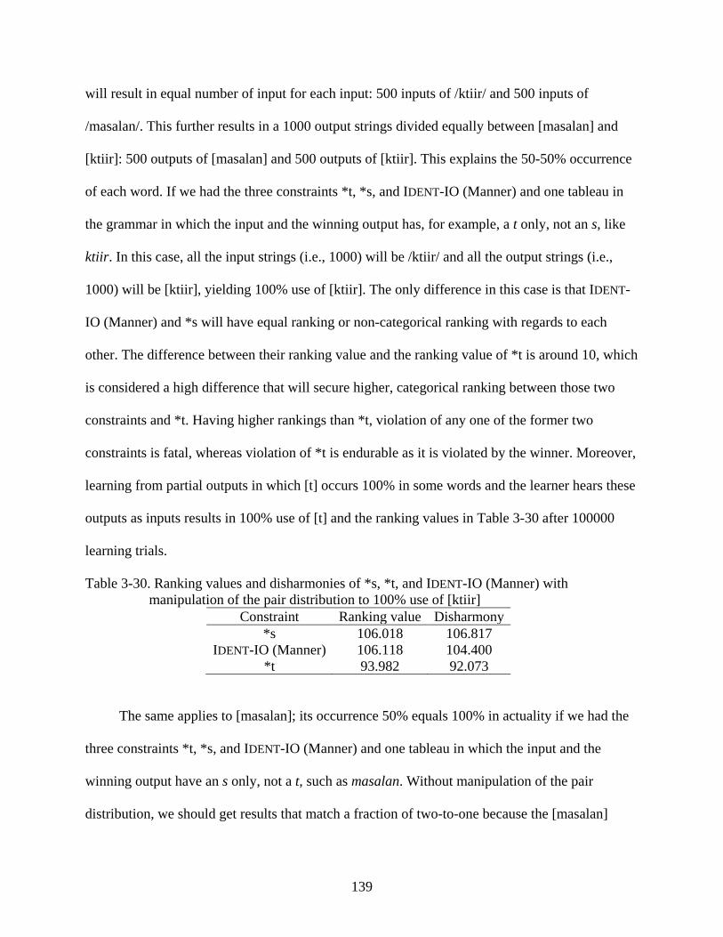
139
will result in equal number of input for each input: 500 inputs of /ktiir/ and 500 inputs of
/masalan/. This further results in a 1000 output strings divided equally between [masalan] and
[ktiir]: 500 outputs of [masalan] and 500 outputs of [ktiir]. This explains the 50-50% occurrence
of each word. If we had the three constraints *t, *s, and IDENT-IO (Manner) and one tableau in
the grammar in which the input and the winning output has, for example, a t only, not an s, like
ktiir. In this case, all the input strings (i.e., 1000) will be /ktiir/ and all the output strings (i.e.,
1000) will be [ktiir], yielding 100% use of [ktiir]. The only difference in this case is that IDENT-
IO (Manner) and *s will have equal ranking or non-categorical ranking with regards to each
other. The difference between their ranking value and the ranking value of *t is around 10, which
is considered a high difference that will secure higher, categorical ranking between those two
constraints and *t. Having higher rankings than *t, violation of any one of the former two
constraints is fatal, whereas violation of *t is endurable as it is violated by the winner. Moreover,
learning from partial outputs in which [t] occurs 100% in some words and the learner hears these
outputs as inputs results in 100% use of [t] and the ranking values in Table 3-30 after 100000
learning trials.
Table 3-30. Ranking values and disharmonies of *s, *t, and IDENT-IO (Manner) with manipulation of the pair distribution to 100% use of [ktiir]
Constraint Ranking value Disharmony *s 106.018 106.817
IDENT-IO (Manner) 106.118 104.400 *t 93.982 92.073
The same applies to [masalan]; its occurrence 50% equals 100% in actuality if we had the
three constraints *t, *s, and IDENT-IO (Manner) and one tableau in which the input and the
winning output have an s only, not a t, such as masalan. Without manipulation of the pair
distribution, we should get results that match a fraction of two-to-one because the [masalan]
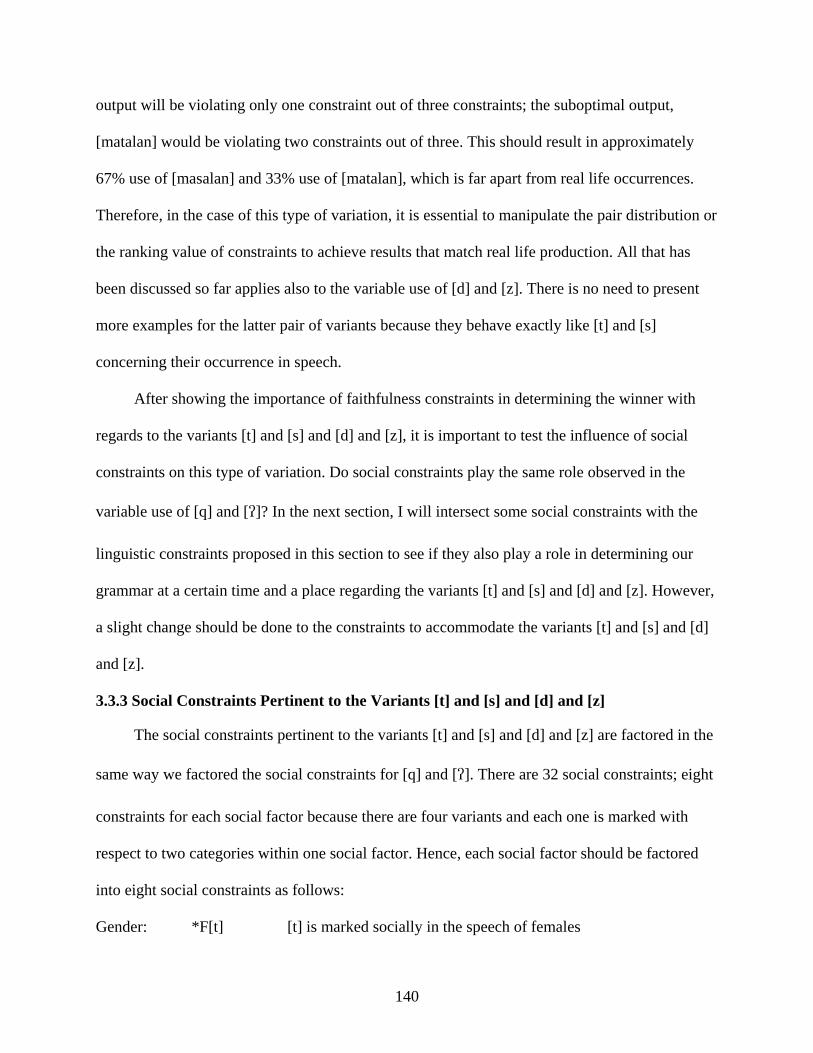
140
output will be violating only one constraint out of three constraints; the suboptimal output,
[matalan] would be violating two constraints out of three. This should result in approximately
67% use of [masalan] and 33% use of [matalan], which is far apart from real life occurrences.
Therefore, in the case of this type of variation, it is essential to manipulate the pair distribution or
the ranking value of constraints to achieve results that match real life production. All that has
been discussed so far applies also to the variable use of [d] and [z]. There is no need to present
more examples for the latter pair of variants because they behave exactly like [t] and [s]
concerning their occurrence in speech.
After showing the importance of faithfulness constraints in determining the winner with
regards to the variants [t] and [s] and [d] and [z], it is important to test the influence of social
constraints on this type of variation. Do social constraints play the same role observed in the
variable use of [q] and []? In the next section, I will intersect some social constraints with the
linguistic constraints proposed in this section to see if they also play a role in determining our
grammar at a certain time and a place regarding the variants [t] and [s] and [d] and [z]. However,
a slight change should be done to the constraints to accommodate the variants [t] and [s] and [d]
and [z].
3.3.3 Social Constraints Pertinent to the Variants [t] and [s] and [d] and [z]
The social constraints pertinent to the variants [t] and [s] and [d] and [z] are factored in the
same way we factored the social constraints for [q] and []. There are 32 social constraints; eight
constraints for each social factor because there are four variants and each one is marked with
respect to two categories within one social factor. Hence, each social factor should be factored
into eight social constraints as follows:
Gender: *F[t] [t] is marked socially in the speech of females
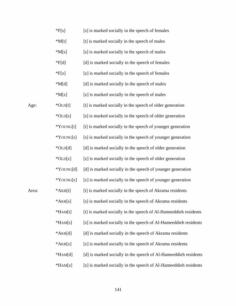
141
*F[s] [s] is marked socially in the speech of females
*M[t] [t] is marked socially in the speech of males
*M[s] [s] is marked socially in the speech of males
*F[d] [d] is marked socially in the speech of females
*F[z] [z] is marked socially in the speech of females
*M[d] [d] is marked socially in the speech of males
*M[z] [z] is marked socially in the speech of males
Age: *OLD[t] [t] is marked socially in the speech of older generation
*OLD[s] [s] is marked socially in the speech of older generation
*YOUNG[t] [t] is marked socially in the speech of younger generation
*YOUNG[s] [s] is marked socially in the speech of younger generation
*OLD[d] [d] is marked socially in the speech of older generation
*OLD[z] [z] is marked socially in the speech of older generation
*YOUNG[d] [d] is marked socially in the speech of younger generation
*YOUNG[z] [z] is marked socially in the speech of younger generation
Area: *AKR[t] [t] is marked socially in the speech of Akrama residents
*AKR[s] [s] is marked socially in the speech of Akrama residents
*HAM[t] [t] is marked socially in the speech of Al-Hameeddieh residents
*HAM[s] [s] is marked socially in the speech of Al-Hameeddieh residents
*AKR[d] [d] is marked socially in the speech of Akrama residents
*AKR[z] [z] is marked socially in the speech of Akrama residents
*HAM[d] [d] is marked socially in the speech of Al-Hameeddieh residents
*HAM[z] [z] is marked socially in the speech of Al-Hameeddieh residents
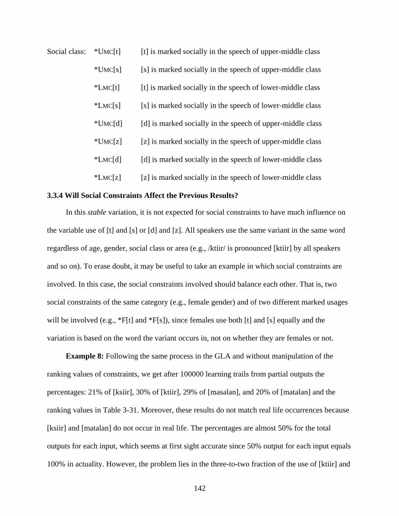
142
Social class: *UMC[t] [t] is marked socially in the speech of upper-middle class
*UMC[s] [s] is marked socially in the speech of upper-middle class
*LMC[t] [t] is marked socially in the speech of lower-middle class
*LMC[s] [s] is marked socially in the speech of lower-middle class
*UMC[d] [d] is marked socially in the speech of upper-middle class
*UMC[z] [z] is marked socially in the speech of upper-middle class
*LMC[d] [d] is marked socially in the speech of lower-middle class
*LMC[z] [z] is marked socially in the speech of lower-middle class
3.3.4 Will Social Constraints Affect the Previous Results?
In this stable variation, it is not expected for social constraints to have much influence on
the variable use of [t] and [s] or [d] and [z]. All speakers use the same variant in the same word
regardless of age, gender, social class or area (e.g., /ktiir/ is pronounced [ktiir] by all speakers
and so on). To erase doubt, it may be useful to take an example in which social constraints are
involved. In this case, the social constraints involved should balance each other. That is, two
social constraints of the same category (e.g., female gender) and of two different marked usages
will be involved (e.g., *F[t] and *F[s]), since females use both [t] and [s] equally and the
variation is based on the word the variant occurs in, not on whether they are females or not.
Example 8: Following the same process in the GLA and without manipulation of the
ranking values of constraints, we get after 100000 learning trails from partial outputs the
percentages: 21% of [ksiir], 30% of [ktiir], 29% of [masalan], and 20% of [matalan] and the
ranking values in Table 3-31. Moreover, these results do not match real life occurrences because
[ksiir] and [matalan] do not occur in real life. The percentages are almost 50% for the total
outputs for each input, which seems at first sight accurate since 50% output for each input equals
100% in actuality. However, the problem lies in the three-to-two fraction of the use of [ktiir] and
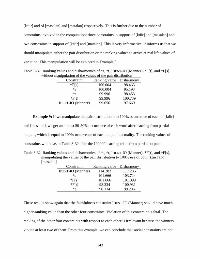
143
[ksiir] and of [masalan] and [matalan] respectively. This is further due to the number of
constraints involved in the computation: three constraints in support of [ktiir] and [masalan] and
two constraints in support of [ksiir] and [matalan]. This is very informative; it informs us that we
should manipulate either the pair distribution or the ranking values to arrive at real life values of
variation. This manipulation will be explored in Example 9.
Table 3-31. Ranking values and disharmonies of *s, *t, IDENT-IO (Manner), *F[t], and *F[s] without manipulation of the values of the pair distribution
Constraint Ranking value Disharmony *F[s] 100.004 98.465
*s 100.004 95.193 *t 99.996 98.453
*F[t] 99.996 100.739 IDENT-IO (Manner) 99.656 97.660
Example 9: If we manipulate the pair distribution into 100% occurrence of each of [ktiir]
and [masalan], we get an almost 50-50% occurrence of each word after learning from partial
outputs, which is equal to 100% occurrence of each output in actuality. The ranking values of
constraints will be as in Table 3-32 after the 100000 learning trials from partial outputs.
Table 3-32. Ranking values and disharmonies of *s, *t, IDENT-IO (Manner), *F[t], and *F[s], manipulating the values of the pair distribution to 100% use of both [ktiir] and [masalan]
Constraint Ranking value Disharmony IDENT-IO (Manner) 114.282 117.236
*s 101.666 103.724 *F[s] 101.666 101.099 *F[t] 98.334 100.931
*t 98.334 99.206
These results show again that the faithfulness constraint IDENT-IO (Manner) should have much
higher-ranking value than the other four constraints. Violation of this constraint is fatal. The
ranking of the other four constraints with respect to each other is irrelevant because the winners
violate at least two of them. From this example, we can conclude that social constraints are not
144
very important in determining our grammar with respect to the variable use of [t] and [s] and [d]
and [z]. What are important in this type of stable variation are faithfulness constraints; these
constraints play a major role in maintaining an equal corresponding output to the input.
3.3.2.1 Concluding remarks on the stable variation among [t] and [s] and [d] and [z]
In conclusion, Examples 8 and 9 show that the inclusion and exclusion of social constraints
regarding the use of the four sounds [t] and [s] and [d] and [z] do not make a difference. Whether
the social constraints *F[s] and *F[t] are included or not, the results are the same (i.e., the
faithfulness constraint is higher ranked than the other constraints (social or linguistic) to preserve
the input in the output). Thus, IDENT-IO (Manner) plays a major role in determining the winners;
it must always have a higher-ranking value than the other markedness constraints to ensure the
observed stable variation between [t] and [s] as well as between [d] and [z]. However, this kind
of lexical conditioning could still be attributed to markedness because even when someone is
reading (which is the case of one speaker who was reading a document to his cousin during the
recording), the person uses [s] instead of []. This presents evidence that speakers prefer less
marked sounds and use them even in casual reading. In other words, speakers may find it easier
to access sounds in their native phonemic inventory and use them instead of those learned later
on in life (i.e., access /s/ and use its surface form [s] rather than use [] that was learned through
formal education of SA as a second language).
145
CHAPTER 4 QUANTITATIVE ANALYSES OF [q] VS. []
4.1 Introduction
In this chapter, I present quantitative analyses for the observed variation in the use of [q]
and []. The purpose of these quantitative analyses is to examine associations and correlations
between both the dependent variants and the independent variables. First, I present tests of
association that could inform us on what determines social class in the city of Hims. Next, a
Bivariate test will be performed on the two dependent variants – [q] and [] – to see if they are
correlated. To examine the main effects of and the interaction effects among the four
independent variables – age, gender, residential area, and social class – on the variable use of [q]
and [], I apply a number of statistical methods. These statistical procedures will help understand
which of these four social factors plays a major or a minor role in the variation. Such
investigations may help in confirming the findings of the theoretical analysis in Chapter 3. A
number of statistical procedures are required for each variant as the following sections will
reveal. The chapter will conclude with a discussion of the findings of the statistical analyses,
trying to relate these findings to previous studies and the findings in Chapter 3. It will also
present implications of these findings.
4.2 Tests of Association of Social Class with Education, Income, Residential Area, and Occupation
These tests are important because social class is a very hazy concept in the Arab World;
many factors may play a role in determining someone’s class. In addition, the social mobility
existent in most societies affects a person’s classification within one social class or another
(Haeri 1996; Labov 2001). This is particularly true of Arab societies because of the great influx
of migration from rural areas to urban centers. Most urban centers are associated with more
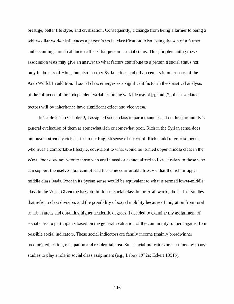
146
prestige, better life style, and civilization. Consequently, a change from being a farmer to being a
white-collar worker influences a person’s social classification. Also, being the son of a farmer
and becoming a medical doctor affects that person’s social status. Thus, implementing these
association tests may give an answer to what factors contribute to a person’s social status not
only in the city of Hims, but also in other Syrian cities and urban centers in other parts of the
Arab World. In addition, if social class emerges as a significant factor in the statistical analysis
of the influence of the independent variables on the variable use of [q] and [], the associated
factors will by inheritance have significant effect and vice versa.
In Table 2-1 in Chapter 2, I assigned social class to participants based on the community’s
general evaluation of them as somewhat rich or somewhat poor. Rich in the Syrian sense does
not mean extremely rich as it is in the English sense of the word. Rich could refer to someone
who lives a comfortable lifestyle, equivalent to what would be termed upper-middle class in the
West. Poor does not refer to those who are in need or cannot afford to live. It refers to those who
can support themselves, but cannot lead the same comfortable lifestyle that the rich or upper-
middle class leads. Poor in its Syrian sense would be equivalent to what is termed lower-middle
class in the West. Given the hazy definition of social class in the Arab world, the lack of studies
that refer to class division, and the possibility of social mobility because of migration from rural
to urban areas and obtaining higher academic degrees, I decided to examine my assignment of
social class to participants based on the general evaluation of the community to them against four
possible social indicators. These social indicators are family income (mainly breadwinner
income), education, occupation and residential area. Such social indicators are assumed by many
studies to play a role in social class assignment (e.g., Labov 1972a; Eckert 1991b).
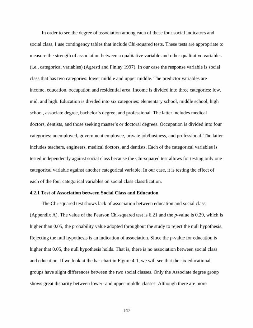
147
In order to see the degree of association among each of these four social indicators and
social class, I use contingency tables that include Chi-squared tests. These tests are appropriate to
measure the strength of association between a qualitative variable and other qualitative variables
(i.e., categorical variables) (Agresti and Finlay 1997). In our case the response variable is social
class that has two categories: lower middle and upper middle. The predictor variables are
income, education, occupation and residential area. Income is divided into three categories: low,
mid, and high. Education is divided into six categories: elementary school, middle school, high
school, associate degree, bachelor’s degree, and professional. The latter includes medical
doctors, dentists, and those seeking master’s or doctoral degrees. Occupation is divided into four
categories: unemployed, government employee, private job/business, and professional. The latter
includes teachers, engineers, medical doctors, and dentists. Each of the categorical variables is
tested independently against social class because the Chi-squared test allows for testing only one
categorical variable against another categorical variable. In our case, it is testing the effect of
each of the four categorical variables on social class classification.
4.2.1 Test of Association between Social Class and Education
The Chi-squared test shows lack of association between education and social class
(Appendix A). The value of the Pearson Chi-squared test is 6.21 and the p-value is 0.29, which is
higher than 0.05, the probability value adopted throughout the study to reject the null hypothesis.
Rejecting the null hypothesis is an indication of association. Since the p-value for education is
higher that 0.05, the null hypothesis holds. That is, there is no association between social class
and education. If we look at the bar chart in Figure 4-1, we will see that the six educational
groups have slight differences between the two social classes. Only the Associate degree group
shows great disparity between lower- and upper-middle classes. Although there are more
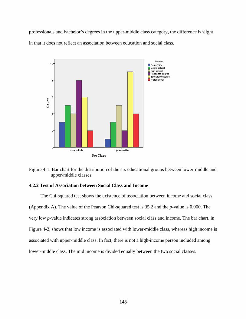
148
professionals and bachelor’s degrees in the upper-middle class category, the difference is slight
in that it does not reflect an association between education and social class.
Figure 4-1. Bar chart for the distribution of the six educational groups between lower-middle and upper-middle classes
4.2.2 Test of Association between Social Class and Income
The Chi-squared test shows the existence of association between income and social class
(Appendix A). The value of the Pearson Chi-squared test is 35.2 and the p-value is 0.000. The
very low p-value indicates strong association between social class and income. The bar chart, in
Figure 4-2, shows that low income is associated with lower-middle class, whereas high income is
associated with upper-middle class. In fact, there is not a high-income person included among
lower-middle class. The mid income is divided equally between the two social classes.
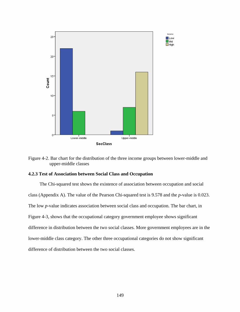
149
Figure 4-2. Bar chart for the distribution of the three income groups between lower-middle and upper-middle classes
4.2.3 Test of Association between Social Class and Occupation
The Chi-squared test shows the existence of association between occupation and social
class (Appendix A). The value of the Pearson Chi-squared test is 9.578 and the p-value is 0.023.
The low p-value indicates association between social class and occupation. The bar chart, in
Figure 4-3, shows that the occupational category government employee shows significant
difference in distribution between the two social classes. More government employees are in the
lower-middle class category. The other three occupational categories do not show significant
difference of distribution between the two social classes.

150
Figure 4-3. Bar chart for the distribution of the four occupational groups between lower-middle
and upper-middle classes
4.2.4 Test of Association between Social Class and Residential Area
The Chi-squared test shows the existence of association between residential area and social
class (Appendix A). The value of the Pearson Chi-squared test is 10.317 and the p-value is 0.001.
The very low p-value indicates strong association between social class and residential area. The
bar chart, in Figure 4-4, shows that much more upper-middle class people live in Al-Hameedieh
than in Akrama. On the other hand, the number of lower-middle class people living in Al-
Hameeddieh and Akrama is not much different.
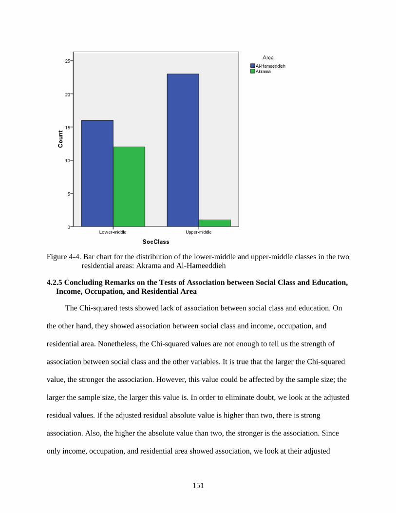
151
Figure 4-4. Bar chart for the distribution of the lower-middle and upper-middle classes in the two
residential areas: Akrama and Al-Hameeddieh
4.2.5 Concluding Remarks on the Tests of Association between Social Class and Education, Income, Occupation, and Residential Area
The Chi-squared tests showed lack of association between social class and education. On
the other hand, they showed association between social class and income, occupation, and
residential area. Nonetheless, the Chi-squared values are not enough to tell us the strength of
association between social class and the other variables. It is true that the larger the Chi-squared
value, the stronger the association. However, this value could be affected by the sample size; the
larger the sample size, the larger this value is. In order to eliminate doubt, we look at the adjusted
residual values. If the adjusted residual absolute value is higher than two, there is strong
association. Also, the higher the absolute value than two, the stronger is the association. Since
only income, occupation, and residential area showed association, we look at their adjusted
152
residuals (Appendix A) to see which one of them has the strongest association. Income has an
adjusted residual absolute value of 5.4 for low income; 5.2 for high income; and only 0.6 for mid
income. Occupation has an adjusted residual absolute value of 3 for government employee; 0.7
for unemployed; 1.2 and 1.3 for business/private job and professional respectively. Residential
area has an adjusted residual absolute value of 3.2 for each of the residential areas. In this sense,
income shows the strongest association followed by residential area. Occupation has the smallest
association; there is only strong association with the government employee category. This fact
was observed in the bar chart in Figure 4-3.
These results are confirmed by the Pearson correlation coefficient, which has the symbol
R. The value of R is usually between -1 and 1; the closer the value to -1 or 1, the stronger the
association. If the value is close to 0, the association is weak. The value of R for education is 0.2,
indicating lack of association. The value of R for income is 0.82, indicating strong association.
The value of R for occupation is 0.1, indicating lack of association. This last result contradicts
the Chi-squared test result for occupation. Hence, one should consider other statistics in addition
to the Chi-squared value and p-value to determine the strength of association. The value of R for
residential area is 0.45, indicating moderate association. The R values for the different
categorical variables investigated for strength of association with social class correlate with the
adjusted residuals results. According to both the R values and the adjusted residual values,
income has the strongest association, followed by residential area. Occupation and education
have no association with social class according to the R values; occupation only shows
significant association with respect to the government employee category according to the
adjusted residual values.
153
In conclusion, one can assume that social class is mainly determined by income and area of
residence in urban centers in the Arab World. It is slightly affected by occupation. Education
does not seem to be a good determining factor of social class. These findings may be helpful for
other researchers who tend to study the influence of social class on linguistic variation in the
Arab World. They could be a starting point for further investigation in urban center, not only in
Syria, but also in other Arab countries.
4.3. Speakers’ Distribution of [q] and []
Before applying statistical procedures to the data to see the effect of the four social factors
on the variable use of [q] and [], I present the distribution of [q] and [] in the speech of each
speaker in Table 4-1. Table 4-1 shows the number of occurrence of each sound from the total
number of sounds for each speaker under the columns [q] and []. Next to each of these columns,
the percentage of the occurrence of each sound is calculated and presented under the percentage
columns. The speakers’ distribution regarding the four factors tested for effect on the observed
variation is also included under separate columns for each factor. Table 4-1 shows that the total
number of tokens for [q] and [] is 11,548. 5874 tokens of [q], which constitute 51% of the total
number of tokens; 5674 tokens of [], which constitute 49% of the total number of tokens.
I entered the information included in Table 4-1 into SPSS to examine the effect of age,
gender, residential area, and social class on the variable use of [q] and []. I created two separate
SPSS data files to perform different tests. I entered social factors in the same way in both data
files. Each of the social factors contains two categories and is entered as a nominal variable. Age
is assigned 1 for the younger age group and 2 for the older age group. Gender is assigned 1 for
females and 2 for males. Residential area is assigned 1 for Al-Hameeddieh and 2 for Akrama.
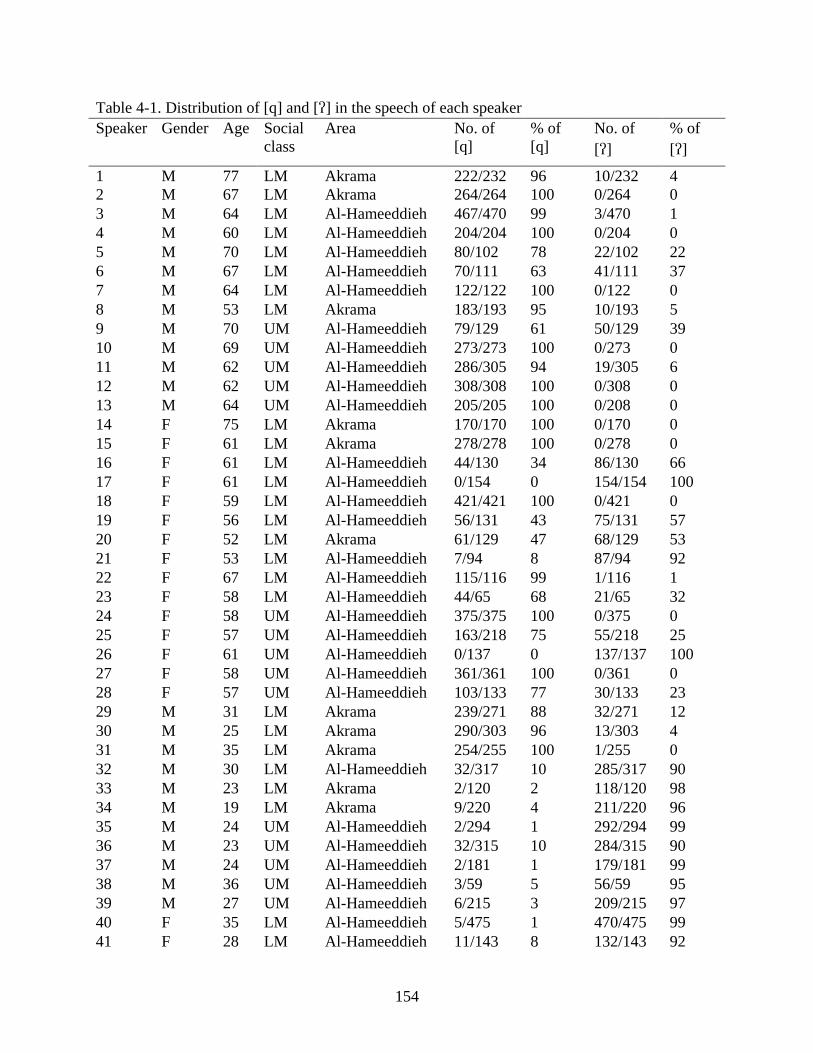
154
Table 4-1. Distribution of [q] and [] in the speech of each speaker Speaker Gender Age Social
class Area No. of
[q] % of [q]
No. of []
% of []
1 M 77 LM Akrama 222/232 96 10/232 4 2 M 67 LM Akrama 264/264 100 0/264 0 3 M 64 LM Al-Hameeddieh 467/470 99 3/470 1 4 M 60 LM Al-Hameeddieh 204/204 100 0/204 0 5 M 70 LM Al-Hameeddieh 80/102 78 22/102 22 6 M 67 LM Al-Hameeddieh 70/111 63 41/111 37 7 M 64 LM Al-Hameeddieh 122/122 100 0/122 0 8 M 53 LM Akrama 183/193 95 10/193 5 9 M 70 UM Al-Hameeddieh 79/129 61 50/129 39 10 M 69 UM Al-Hameeddieh 273/273 100 0/273 0 11 M 62 UM Al-Hameeddieh 286/305 94 19/305 6 12 M 62 UM Al-Hameeddieh 308/308 100 0/308 0 13 M 64 UM Al-Hameeddieh 205/205 100 0/208 0 14 F 75 LM Akrama 170/170 100 0/170 0 15 F 61 LM Akrama 278/278 100 0/278 0 16 F 61 LM Al-Hameeddieh 44/130 34 86/130 66 17 F 61 LM Al-Hameeddieh 0/154 0 154/154 100 18 F 59 LM Al-Hameeddieh 421/421 100 0/421 0 19 F 56 LM Al-Hameeddieh 56/131 43 75/131 57 20 F 52 LM Akrama 61/129 47 68/129 53 21 F 53 LM Al-Hameeddieh 7/94 8 87/94 92 22 F 67 LM Al-Hameeddieh 115/116 99 1/116 1 23 F 58 LM Al-Hameeddieh 44/65 68 21/65 32 24 F 58 UM Al-Hameeddieh 375/375 100 0/375 0 25 F 57 UM Al-Hameeddieh 163/218 75 55/218 25 26 F 61 UM Al-Hameeddieh 0/137 0 137/137 100 27 F 58 UM Al-Hameeddieh 361/361 100 0/361 0 28 F 57 UM Al-Hameeddieh 103/133 77 30/133 23 29 M 31 LM Akrama 239/271 88 32/271 12 30 M 25 LM Akrama 290/303 96 13/303 4 31 M 35 LM Akrama 254/255 100 1/255 0 32 M 30 LM Al-Hameeddieh 32/317 10 285/317 90 33 M 23 LM Akrama 2/120 2 118/120 98 34 M 19 LM Akrama 9/220 4 211/220 96 35 M 24 UM Al-Hameeddieh 2/294 1 292/294 99 36 M 23 UM Al-Hameeddieh 32/315 10 284/315 90 37 M 24 UM Al-Hameeddieh 2/181 1 179/181 99 38 M 36 UM Al-Hameeddieh 3/59 5 56/59 95 39 M 27 UM Al-Hameeddieh 6/215 3 209/215 97 40 F 35 LM Al-Hameeddieh 5/475 1 470/475 99 41 F 28 LM Al-Hameeddieh 11/143 8 132/143 92
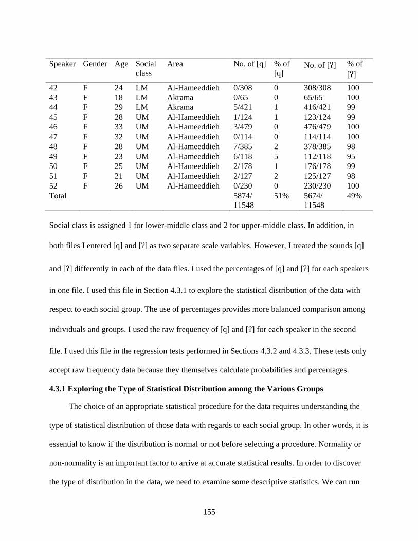
155
Speaker Gender Age Social
class Area No. of [q] % of
[q] No. of [] % of
[] 42 F 24 LM Al-Hameeddieh 0/308 0 308/308 100 43 F 18 LM Akrama 0/65 0 65/65 100 44 F 29 LM Akrama 5/421 1 416/421 99 45 F 28 UM Al-Hameeddieh 1/124 1 123/124 99 46 F 33 UM Al-Hameeddieh 3/479 0 476/479 100 47 F 32 UM Al-Hameeddieh 0/114 0 114/114 100 48 F 28 UM Al-Hameeddieh 7/385 2 378/385 98 49 F 23 UM Al-Hameeddieh 6/118 5 112/118 95 50 F 25 UM Al-Hameeddieh 2/178 1 176/178 99 51 F 21 UM Al-Hameeddieh 2/127 2 125/127 98 52 F 26 UM Al-Hameeddieh 0/230 0 230/230 100 Total 5874/
11548 51% 5674/
11548 49%
Social class is assigned 1 for lower-middle class and 2 for upper-middle class. In addition, in
both files I entered [q] and [] as two separate scale variables. However, I treated the sounds [q]
and [] differently in each of the data files. I used the percentages of [q] and [] for each speakers
in one file. I used this file in Section 4.3.1 to explore the statistical distribution of the data with
respect to each social group. The use of percentages provides more balanced comparison among
individuals and groups. I used the raw frequency of [q] and [] for each speaker in the second
file. I used this file in the regression tests performed in Sections 4.3.2 and 4.3.3. These tests only
accept raw frequency data because they themselves calculate probabilities and percentages.
4.3.1 Exploring the Type of Statistical Distribution among the Various Groups
The choice of an appropriate statistical procedure for the data requires understanding the
type of statistical distribution of those data with regards to each social group. In other words, it is
essential to know if the distribution is normal or not before selecting a procedure. Normality or
non-normality is an important factor to arrive at accurate statistical results. In order to discover
the type of distribution in the data, we need to examine some descriptive statistics. We can run
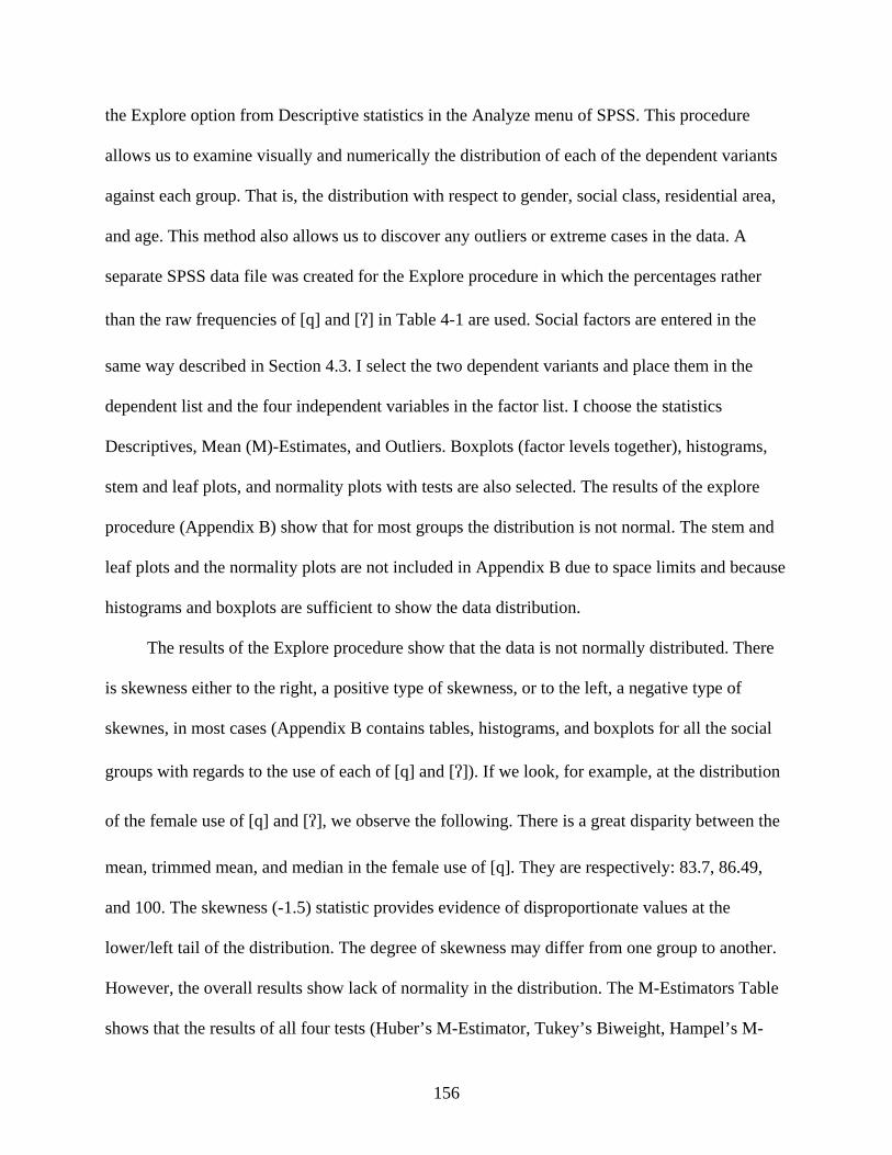
156
the Explore option from Descriptive statistics in the Analyze menu of SPSS. This procedure
allows us to examine visually and numerically the distribution of each of the dependent variants
against each group. That is, the distribution with respect to gender, social class, residential area,
and age. This method also allows us to discover any outliers or extreme cases in the data. A
separate SPSS data file was created for the Explore procedure in which the percentages rather
than the raw frequencies of [q] and [] in Table 4-1 are used. Social factors are entered in the
same way described in Section 4.3. I select the two dependent variants and place them in the
dependent list and the four independent variables in the factor list. I choose the statistics
Descriptives, Mean (M)-Estimates, and Outliers. Boxplots (factor levels together), histograms,
stem and leaf plots, and normality plots with tests are also selected. The results of the explore
procedure (Appendix B) show that for most groups the distribution is not normal. The stem and
leaf plots and the normality plots are not included in Appendix B due to space limits and because
histograms and boxplots are sufficient to show the data distribution.
The results of the Explore procedure show that the data is not normally distributed. There
is skewness either to the right, a positive type of skewness, or to the left, a negative type of
skewnes, in most cases (Appendix B contains tables, histograms, and boxplots for all the social
groups with regards to the use of each of [q] and []). If we look, for example, at the distribution
of the female use of [q] and [], we observe the following. There is a great disparity between the
mean, trimmed mean, and median in the female use of [q]. They are respectively: 83.7, 86.49,
and 100. The skewness (-1.5) statistic provides evidence of disproportionate values at the
lower/left tail of the distribution. The degree of skewness may differ from one group to another.
However, the overall results show lack of normality in the distribution. The M-Estimators Table
shows that the results of all four tests (Huber’s M-Estimator, Tukey’s Biweight, Hampel’s M-
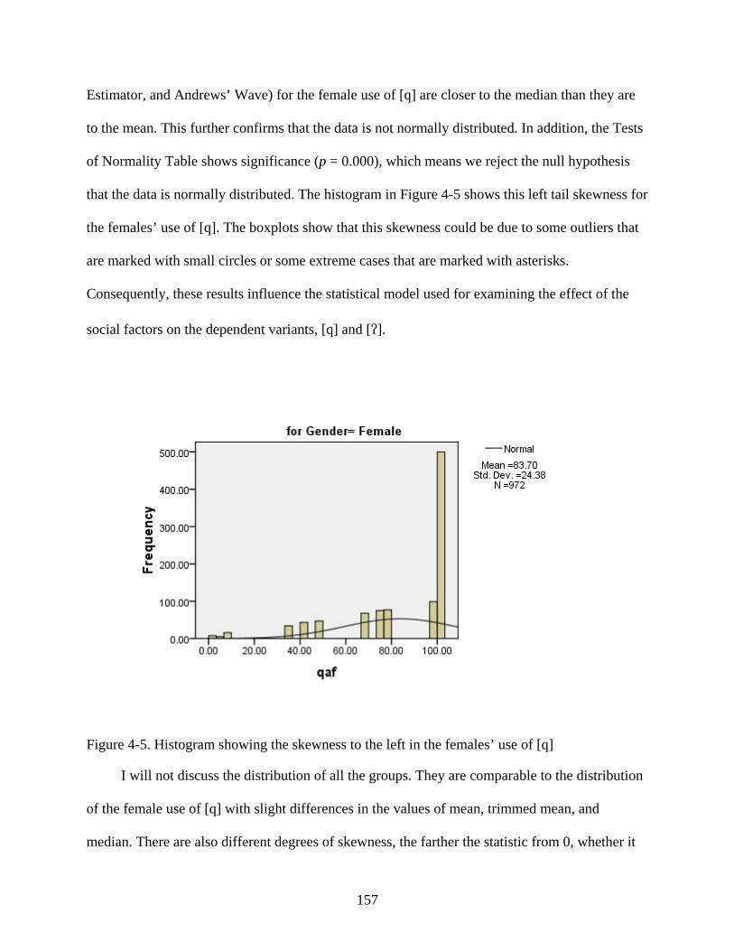
157
Estimator, and Andrews’ Wave) for the female use of [q] are closer to the median than they are
to the mean. This further confirms that the data is not normally distributed. In addition, the Tests
of Normality Table shows significance (p = 0.000), which means we reject the null hypothesis
that the data is normally distributed. The histogram in Figure 4-5 shows this left tail skewness for
the females’ use of [q]. The boxplots show that this skewness could be due to some outliers that
are marked with small circles or some extreme cases that are marked with asterisks.
Consequently, these results influence the statistical model used for examining the effect of the
social factors on the dependent variants, [q] and [].
Figure 4-5. Histogram showing the skewness to the left in the females’ use of [q]
I will not discuss the distribution of all the groups. They are comparable to the distribution
of the female use of [q] with slight differences in the values of mean, trimmed mean, and
median. There are also different degrees of skewness, the farther the statistic from 0, whether it
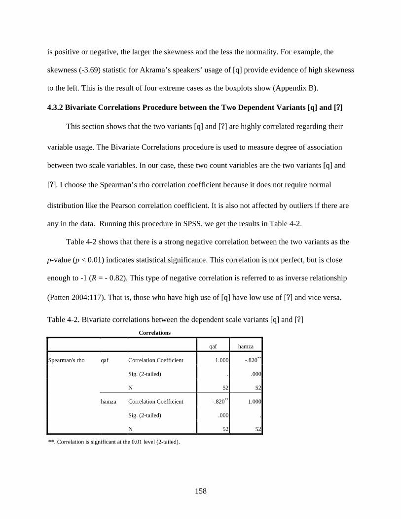
158
is positive or negative, the larger the skewness and the less the normality. For example, the
skewness (-3.69) statistic for Akrama’s speakers’ usage of [q] provide evidence of high skewness
to the left. This is the result of four extreme cases as the boxplots show (Appendix B).
4.3.2 Bivariate Correlations Procedure between the Two Dependent Variants [q] and []
This section shows that the two variants [q] and [] are highly correlated regarding their
variable usage. The Bivariate Correlations procedure is used to measure degree of association
between two scale variables. In our case, these two count variables are the two variants [q] and
[]. I choose the Spearman’s rho correlation coefficient because it does not require normal
distribution like the Pearson correlation coefficient. It is also not affected by outliers if there are
any in the data. Running this procedure in SPSS, we get the results in Table 4-2.
Table 4-2 shows that there is a strong negative correlation between the two variants as the
p-value (p < 0.01) indicates statistical significance. This correlation is not perfect, but is close
enough to -1 (R = - 0.82). This type of negative correlation is referred to as inverse relationship
(Patten 2004:117). That is, those who have high use of [q] have low use of [] and vice versa.
Table 4-2. Bivariate correlations between the dependent scale variants [q] and [] Correlations
qaf hamza
Spearman's rho qaf Correlation Coefficient 1.000 -.820**
Sig. (2-tailed) . .000
N 52 52
hamza Correlation Coefficient -.820** 1.000
Sig. (2-tailed) .000 .
N 52 52
**. Correlation is significant at the 0.01 level (2-tailed).

159
4.3.3 Generalized Linear Models (GZLM) Procedure for the Effect of the Four Independent Variables on the Two Dependent Variants [q] and []
The GZLM includes statistical procedures such as linear regression for normally
distributed response variables, logistic models for binary response or event count data, and
loglinear models for event count responses. One can also use a mix of statistical models through
the very general model formulation. The GZLM allow us to measure the main effects of one or
more independent variables on a dependent variable. In our case, the independent variables are
four: age, gender, residential area, and social class. The dependent variants are [q] and []. The
GZLM also allow us to measure the effect of interaction among the independent variables on the
dependent variable. The general linear model (GLM) multivariate procedure allows us to
measure the main effects and interaction of a number of independent variables on one or more
dependent variables through a multivariate test. The GLM, however, assumes normal distribution
and constant variance. The GZLM, thus, has an advantage over the GLM. They do not
necessarily “assume a normal distribution or constant variance” (Agresti and Finlay 1997: 550).
Having discovered in Section 4.2.1 that the distribution of the dependent variants among the
different groups is not normal, it is more appropriate to use one of the GZLM. In addition to
allowing non-normal distribution, the GZLM expands the GLM by specifying a link function
that relates the dependent variable linearly to the independent variables.
To choose the appropriate GZLM model, we check the type of data in addition to the
distribution. In this study, the data are count. Count data refer to the number of events of a
number of trials. The number of events in my data is the number of occurrence of each of the two
dependent variants in the speech of each speaker. The number of trials is the total number of
occurrences for all speakers/subjects for each variant. The number of trials, in my data, is the
fixed value 5874 for the [q] variant and 5674 for the [] variant (Table 4-1). One can use binary

160
logistic to account for count data by specifying the fixed value of the variable (i.e., the total
number of trials) for each variant, rather than treating the variant as binary. However, a Poisson
distribution is more commonly used for non-normally distributed count response variable. The
link function that is appropriate for count data and is usually used with a Poisson distribution is a
Log link. The Log link, unlike the identity link, allows the mean to relate non-linearly to the
independent variables. The Log link is often referred to as loglinear model. Hence, my initial
choice of procedure for my statistical analysis is the Poisson loglinear regression, which is one
type of regression tests that are used in probabilistic linguistics for count data (Manning
2003:335).
However, after performing the Poisson loglinear procedure, I realized that in the Goodness
of Fit Table (Appendix C) that the Deviance and the Pearson Chi-squared (4798.992 and
5687.238 respectively) are too high. The value/df is also too high (102.106 for the Deviance and
121.005 for the Pearson Chi-squared), indicating overdispersion of the data. The value/df should
be close to 1. If it is higher than 1, it could still indicate a good fit of the model. However, if it is
too high, it indicates overdispersion and probably the need for a better fitting model for
overdispersion. In addition, the Log Likelihood is too low (-2527.807). The Akaike's Information
Criterion (AIC) (5065.613) and the Bayesian Information Criterion (BIC) (5075.369) are also too
high. The smaller the AIC and BIC, the better the fit. The values of the Deviance, Pearson Chi-
squared, Log Likelihood, the value/df, AIC, and BIC cast doubt on the goodness-of-fit of the
model, although the Likelihood ratio Chi-squared (G2) value (28.042) in the Omnibus Test Table
shows significance (p = 0.000). The observed significance of the G2 means that we can reject the
null hypothesis that the independent variables have no effect on the variable use of the dependent
variant [q]. To evade this doubt, I checked the goodness-of-fit criteria of the standard Poisson
161
regression procedure against those of a negative binomial regression procedure with all other
settings equal. Usually, negative binomial regression is recommended for overdispersed data. By
changing the type of model to negative binomial with Log link, we actually get a better fitting
model. The Log Likelihood (Appendix C) becomes higher (-265.034), and the value/df is higher
than 1, but not extremely higher than one (1.932 for the deviance and 1.598 for the Pearson Chi-
squared). In addition, the Deviance and the Pearson Chi-squared (90.806 and 75.09 respectively)
are much smaller. The AIC (540.068) and BIC (549.825) are also much smaller than those in the
Poisson regression. The Omnibus Test Table also shows significance (p = 0.000) of the G2 value
(41.313). In other words, the negative binomial procedure also rejects the null hypothesis and
indicates that at least some of the social factors influence the variable use of [q]. Since both
Poisson and negative binomial regressions show significant G2 values, negative binomial
regression provides a better fit for the overdispersed data by having other supporting goodness-
of-fit criteria.
4.3.3.1 Negative binomial regression showing the main effects of the four independent variables, age, gender, residential area, and social class, on the variable use of the dependent variant [q]
In this section, mainly age and gender emerge as significant. Although residential area
emerges as significant in one test, it shows otherwise in another test. On the other hand, social
class emerges as insignificant. The negative binomial regression procedure is run though the
SPSS software. From the analyze menu, I choose Generalized Linear Models. Then, I choose
negative binomial regression as the type of model. Like the Poisson regression, negative
binomial assumes non-normal distribution of the count data and the link function Log. For the
response variable, I choose [q]. For the predictors, I choose the four independent variables as
factors: social class, age, gender, and residential area. From options, I choose descending. For the
model, I choose first the main effects of the four factors to see the effect of each independent
162
variable on the response variable independently. For the estimation, I use the Pearson Chi-
squared scale parameter method. This method is better for overdispersed data. For statistics, I
check the case processing summary statistics, descriptive statistics, model information, goodness
of fit, model summary statistics, and parameter estimates including exponential parameter
estimates. Under the estimated mean (EM)-estimates, I select all four factors to measure simple
contrast between each of the two categories included in the factor (e.g., contrast between the
female and male categories in the gender factor). I also identify the category of reference, usually
the highest number (2). For example, I chose the [Gender = 2], that is males who have been
assigned to the category 2, as the reference category. Finally, I save the predicted value of linear
predictor and the standardized deviance residual. These values are saved to the active data base
and later used in a scatter plot to perform an informal model check. From graphs, I select simple
scatter plot and drag it to the open window. The predicted value of linear predictor is dragged to
the horizontal/X-axis and the standardized deviance residual is dragged to the vertical/Y-axis.
The resultant plot should show us if there are any outliers.
The results of the negative binomial regression (Appendix C) show in the Tests of Model
Effects Table that age (p = 0.000), gender (p = 0.009), and residential area (p = 0.008) play
significant roles in the observed variation in the use of [q]. In contrast, social class (p = 0.862) do
not seem to play a significant role in the variable use of [q]. The role played by age seems to be
more important than the role played by gender and residential area. In the Parameter Estimate
Table, we can read the coefficients under the column entitled B. These coefficients enable us to
interpret the degree of use of each variant by the various groups of speakers. We can also read
the exponential of the coefficient B under the column entitled Exp(B), which tells us the odds
ratio of the occurrence of a certain sound in the speech of a group of speakers. The B coefficient
163
for age is 2.866; it is positive. This means that older speakers [Age = 2] use more [q] than
younger speaker [Age = 1]. The Exp(B) for age is 17.564. This number informs us that the odds
that older speakers would use the [q] are 18 times the odds that the younger speakers would use
the [q]. The coefficient for gender is 1.117; it is also positive. This means that males [Gender =
2] use more [q] than females [Gender = 1]. The Exp(B) for gender is 3.055. This number informs
us that the odds that males would use the [q] are 3 times the odds that females would use the [q].
The coefficient for residential area is 1.481; it is also positive. This means that Akrama speakers
[Area = 2] use more [q] than Al-Hameeddieh speakers [Area = 1]. The Exp(B) for residential
area is 4.398. This number informs us that the odds that Akrama speakers would use the [q] are 4
times the odds that Al-Hameeddieh speakers would use the [q]. Although social class did not
show significant effects, reading the coefficient may reveal some variation between the two
social classes in their use of [q]. Speakers from the upper-middle class use [q] slightly less than
speakers from the lower-middle class (coefficient B = - 0.072). The Exp(B) for social class is
0.93. This number informs us that the odds that upper-middle class would use the [q] are 93% of
the odds/amount that lower-middle class would use the [q]. It is also useful to look at the
estimated marginal means that result from the simple contrast performed on the two categories
within each factor. The estimated marginal means indicate the difference between the two
categories within a factor.
Age. With regards to age, the estimated marginal mean for older speakers is 333.42 and
18.98 for younger speakers. If we multiply 18.98 by the odds ratio, 17.564, we get 333.36. This
result confirms that older speakers use [q] 18 times the amount used by younger speakers. In this
sense, older speakers are expected to use [q] much more than younger speaker do. The Individual
Result Table shows that the difference between older and younger speakers is highly significant
164
(p = 0.003). The Overall Test Table also reports significant contrast between older and younger
speakers (p = 0.003).
Gender. As for Gender, the estimated marginal mean for males is 139.06, whereas it is
45.51 for females. Multiplying 45.51 by the odds ratio, 3.055, we get 139.03, indicating males
are expected to use 3 times what females use. The Individual Result Table displays the
significance (p = 0.023) of this difference between males’ and females’ use of [q]. The Overall
Test Table also reports significant contrast between males and females (p = 0.023).
Residential area. Although the estimated marginal means for residential area show great
difference (166.85 for Akrama speakers and 37.93 for Al-Hameeddieh speakers), this difference
is not significant according to the Individual Result Table and the Overall Test Table. Both tables
report a p-value that is larger than 0.05 (p = 0.092).
Social class. The same applies to social class. The estimated marginal mean for upper-
middle class is 76.74 and 82.48 for lower-middle class). This difference is not significant
according to the Individual Result Table and the Overall Test Table. Both tables report a p-value
that is much larger than 0.05 (p = 0.86).
The significance shown in the contrast tests for age and gender indicate that the variation is
not due to chance; rather, it is a variation that is affected by those two social factors. The
difference is still significant even after the p-values are adjusted by the sequential Sidak method.
However, the insignificance of the contrast test for residential area shows that the variation
between Akrama and Al-Hameeddieh speakers is a chance variation, not necessarily a variation
affected by residential area. Thus, the simple contrast results for all social factors do not
completely accord with the results of the Parameter Estimates Table. Age and gender are
significant predictors of the variable use of [q], but residential area is not as significant.
165
Looking also at the scatter plot resulting from saving the standardized deviance residuals
and the estimated linear predictors, we note that there is strong variability of residuals across all
values of the linear predictor. However, variability increases towards the central value of the
mean and decreases as the mean increases. There may be a possible cause for concern regarding
outliers. There are 3 points that are higher than 2. Usually, residuals that are higher than 2 are
considered outliers. Some sources suggest that for a point to be consider an outlier, it should be
higher than 3 (Agresti and Finlay 1997). In this case, the scatter plot does not show any outliers.
4.3.3.2 Negative binomial regression showing the effect of the interaction of the independent variables, age, gender, and residential area, on the variable use of the dependent variant [q]
In this section, we will see interaction between age, gender, and residential area. However,
this interaction does not hold for all social categories. I apply a three-way interaction model to
see if there is interaction among the social factors that have shown significant main effects in
Section 4.2.3.1. I only exclude social class because it showed the least effect among the four
independent variables. I do not exclude residential area, although it did not show significant
difference between Akrama and Al-Hameeddieh speakers in the contrast test. The three-way
interaction model of the negative binomial regression seems to be more fitting than the main
effects model in Section 4.2.3.1. The Log Likelihood value is (-254.43), which is higher than the
Log Likelihood value of the main effects model (-265.034). The Deviance, Pearson Chi-squared,
AIC, and BIC show smaller values (69.59, 36.965, 524.86, and 540.47 respectively) than the
main effects model. Also, the value/df are smaller than the main effects model (1.582 for
Deviance and 0.84 for Pearson Chi-squared). The Omnibus Test Table also shows significance at
p < 0.05 and the Likelihood ratio Chi-squared is 103.808. The Test of Model Effect Table shows
that age (p = 0.000) and gender (p = 0.000) have significant effects independently from each
other. The p-value for residential area (p = 0.052) approaches significance. Thus, residential area
166
is included in the interaction model. The interaction of age, gender, and area is also statistically
significant (p = 0.000). The Parameter Estimates Table shows that age (p = 0.000), gender (p =
0.007) and the interaction between the [Age=1], [Gender=2], and [Area=2] (younger males from
Akrama) (0.005) are statistically significant. Residential area and other interactions of the
categories within the three factors do not show significance. Looking at the coefficient B values
may, however, be useful in determining the difference between the two categories within a factor
or the interaction between the various categories. The coefficient B for age is (3.734), which
indicates much more use of [q] by the older age group [Age = 2] than the younger age group.
The odds ratio under column Exp(B) shows that the odds that older speakers would use the [q]
sound is 41.845 times the odds that the younger speakers will use the [q] sound. The coefficient
B for gender is (1.339), which indicates much more use of [q] by males [Gender = 2] than
females group. The odds ratio under column Exp(B) shows that the odds that males would use
the [q] sound is 3.815 times the odds that females would use the [q] sound. The interaction
among [Age=1], [Gender=2], and [Area=2] seems to have the highest coefficient B (2.812)
among all other interactions. This means that younger male speakers who reside in Akrama use
more [q] than younger female speakers who reside in Akrama. This is supported by the fact that
in Table 4-1, there are three younger male speakers (29, 30, & 31) who reside in Akrama and use
almost 100% [q], in contrast to younger female speakers from the same area. In addition, the
coefficient (B = 484) of the interaction among [Age=2], [Gender=1], and [Area=2] shows that
older female speakers from Akrama use slightly more [q] than older female speakers from Al-
Hameeddieh and younger female speakers from both Akrama and Al-Hameeddieh.
167
4.3.3.3 Negative binomial regression showing the effect of the interaction of the two independent variables, age and gender, on the variable use of the dependent variant [q]
This section will show strong interaction between age and gender. A two-way interaction
model is employed to investigate this interaction. This model shows a worse fit than the three-
way interaction model discussed in Section 4.2.3.2, but a better fit than the main effects model.
The Log Likelihood value for the two-way interaction is (-261.794). The Omnibus Test Table
shows significance (p = 0.000) and a Likelihood ratio Chi-squared of (71.153). The Test of
Model Effect Table shows that both age (p =0.000) and gender (p = 0.000) have significant
effects independently from each other. The interaction between age and gender is also significant
(p = 0.000). The Parameter Estimates Table shows similar results to the Test of Model Effect
Table. Age (p =0.000) and gender (p = 0.000) are statistically significant as well as the
interaction between gender and age (p = 0.000). The coefficient B (3.815) shows that older age
group uses [q] more than younger age group. The odds ratio shows that the odds that older
speakers would use [q] are 45.356 times the use of [q] by younger speakers. The coefficient B
(3.119) shows that males use [q] more than females. The odds ratio shows that the odds that
males would use [q] are 24.509 times the use of [q] by females. The coefficient B (-2.827) for the
interaction between age and gender shows negative association. That is, older male speakers use
[q] less than older female speakers and younger female and male speakers. The odds ratio shows
that the odds that older male speakers would use [q] are 5.9% of the use of other speakers. This
result does not sound right because my observations of speakers and all the previous statistical
tests show that older speakers and male speakers use more [q] than younger speakers and female
speakers.
168
4.3.3.4 Negative binomial regression showing the main effects of the four independent variables, age, gender, residential area, and social class, on the variable use of the dependent variant []
As it is the case regarding the use of [q], in this section age, gender, and residential area
emerge as significant concerning the use of []. I follow the same procedure of the negative
binomial regression that I followed for [q]. The only difference is that the response variable is []
instead of [q]. In the Goodness-of-Fit Table (Appendix D), Deviance and Pearson Chi-squared
are 104.98 and 50.341 respectively. The value/df are higher than 1 (2.234 for Deviance and
1.071 for Pearson Chi-squared), indicating the fitness of the model for the observed variation.
The Log Likelihood is -268.473. The Omnibus Test Table shows significance at p < 0.05 and a
Likelihood ratio Chi-squared of (51.853), indicating the existence of main effects of at least
some of the independent variables.
The results of the negative binomial regression procedure (Appendix D, Tests of Model
Effects Table) show that age (p = 0.000), gender (p = 0.005), and area (p = 0.035) play
significant roles in the observed variation in the use of []. In contrast, social class (p = 0.321) do
not seem to play a significant role in the variable use of [].The role played by age seems to be
more imprtant than the role played by gender and area. These results are similar to those when
examining the main effects of age, gender, residential area, and social class on the variable use of
[q]. In the Parameter Estimate Table, we can read the coefficients under the column entitled B.
Those coefficients enable us to interpret the degree of use of the variant [] by the various groups
of speakers. The coefficient for age is (-2.186); it is negative. This means that older speakers
[Age = 2] use much less [] than younger speakers [Age =1]. The odds ratio for age (0.112)
shows that the odds that older speakers would use [] is very small (i.e., 1.12% of the amount of
169
use of [] by the younger speakers). The coefficient for gender is (-0.858), which means that
male speakers [Gender = 2] use slightly less [] than female speakers [Gender = 1]. The odds
ratio for gender (0.424) shows that the odds that male speakers would use [] is very small (i.e.,
4.24% of the amount of use of [] by female speakers). The coefficient for area is (-0.887); it is
also negative. This means that speakers from Akrama [Area = 2] use less [] than speakers from
Al-Hameeddieh [Area =1]. The odds ratio for area (0.412) shows that the odds that speakers
from Akrama would use [] is very small (i.e., 4.12% of the amount of use of [] by the speakers
from Al-Hameeddieh). Although social class does not play a significant role in the variation,
reading the coefficient column shows that there is a slight difference between the two social
classes. Speakers from the upper-middle class use [] slightly less than speakers from the lower-
middle class (coefficient B = -0.353). The odds ratio for social class (0.703) shows that the odds
that the upper-middle class would use [] is very small (i.e., 7.03% of the amount of use of [] by
the lower-middle class). It is also useful to look at the estimated marginal means that result from
the simple contrast performed on the two categories within each factor. The estimated marginal
means indicate the difference between the two categories.
Age. With regards to age, the estimated marginal mean for younger speakers is 157.38,
whereas it is 17.68 for older speakers. Thus, younger speakers are expected to use [] much more
than older speakers. Both the Individual Result Table and the Overall Test Table show that the
difference between the two age group in their use of [] is significant (p = 0.000).
Gender. The estimated marginal means for gender also show great difference (81.01 for
female speakers and 34.35 for male speakers). This difference is significant according to the
170
Individual Result Table and the Overall Test Table. Both tables report a p-value smaller than
0.05 (p = 0.017).
Residential area. As for residential area, the estimated marginal mean for Al-Hameeddieh
speakers is 82.2 and 33.85 for Akrama speakers. In this sense, Al-Hameeddieh speakers’ use of
[] is more than double Akrama speakers’ use of it. Both the Individual Result Table and the
Overall Test Table show that the difference Al-Hameeddieh and Akrama speakers is highly
significant (p = 0.016).
Social class. In contrast, the estimated marginal mean do not show a great difference
between the two classes (44.22 for the upper-middle class and 62.93 for the lower-middle class).
This difference is not significant according to the Individual Result Table and the Overall Test
Table. Both tables report a p-value that is larger than 0.05 (p = 0.304).
The significance of age, gender, and area shown in the contrast tests indicate that the
variation is not due to chance; rather, it is a variation that is affected by the three social factors:
age, gender and residential area. The difference is still significant even after the p-values are
adjusted by the sequential Sidak method. Thus, the simple contrast results for all social factors
accord with the results of the Parameter Estimates Table. That is, age, gender, and residential
area are significant predictors of the variable use of [].
Looking also at the scatter plot resulting from saving the standardized deviance residuals
and the estimated linear predictors, we note that there is strong variability of residuals across all
values of the linear predictor. There may be a possible cause for concern regarding outliers.
There are 9 points that are higher than 2. Usually, residuals that are higher than 2 are considered
outliers. Some sources suggest that for a point to be consider an outlier, it should be higher than
3 (Agresti and Finlay 1997). In this case, the scatter plot does not show any outliers.
171
4.3.3.5 Negative binomial regression showing the effect of the interaction of the independent variables, age, gender, and residential area, on the variable use of the dependent variant []
In this section, we note that unlike the case of [q], there is no interaction between age,
gender, and residential area regarding the use of []. Like in the case of [q], I apply a three-way
interaction model to see if there is interaction among the social factors that have shown
significant main effects in Section 4.2.3.4. I only exclude social class because it showed the least
effect among the four independent variables. The three-way interaction model of the negative
binomial regression seem to be more fitting than the main effects model in Section 4.2.3.4. In the
Goodness-of-Fit Table (Appendix D), Deviance and Pearson Chi-squared are 101.808 and
45.578 respectively, which are smaller than the ones in the main effects model and closer to the
degree of freedom (df) value. The value/df are higher than 1 (2.314 for Deviance and 1.036 for
Pearson Chi-squared), which shows smaller dispersion than the main effects model and a better
fit. The Log Likelihood value is (-266.887), which is higher than the Log Likelihood value of the
main effects model. The Omnibus Test Table shows significance at p < 0.05 and a Likelihood
ratio Chi-squared 56.678. The Test of Model Effect Table shows that only age (p = 0.000) and
gender (p = 0.006) are statistically significant. Residential area (p = 0.077) does not have
significant effects. The interaction among the three social factors is also insignificant (p = 0.395).
In the Parameter Estimates Table shows only age (p = 0.000) is statistically significant. Gender
(p = 0.847) and residential area (p = 0.999), in contrast, do not show significance as well as the
interaction among the various categories. The coefficient B for age (-1.496) from the Parameter
Estimates Table shows that older speakers use [] less than younger speakers. The odds ratio for
age shows that the odds that older speakers would use [] is smaller than the odds that the
younger speakers would use [] (i.e., 2.24% of the amount used by younger speakers). Although
172
the other two factors and the interaction among the three factors are not significant, I will discuss
them in terms of what the coefficients show us. It is worth noting that the coefficients and the
odds ratio show that males use less [] than females (B = - 0.1; Exp(B) = 0.905 = 9.05% of the
females use of []). The coefficients and the odds ratio show that younger males from Akrama
use less [] than younger males from Al-Hameedieh (B = - 1.065; Exp(B) = 0.345 = 3.45% of the
use of [] by younger males from Al-Hameeddieh). In addition, older female speakers form
Akrama use less [] than older females from Al-Hameedieh and younger female speakers from
both Akrama and Al-Hameeddieh (B = - 0.866; Exp(B) = 0.421 = 4.21% of the other females’
use of []).
4.3.3.6 Negative binomial regression showing the effect of the interaction of the two independent variables, age and gender, on the variable use of the dependent variant []
This section will also show that unlike the case of [q], there is no interaction between age
and gender regarding the use of []. A two-way interaction model has a worse fit than both the
main effects model and the three-way interaction. In the Goodness-of-Fit Table (Appendix D),
Deviance and Pearson Chi-squared are 107.027 and 48.573 respectively, which are higher than
the other two models. The value/df are higher than 1 (2.23 for Deviance and 1.012 for Pearson
Chi-squared), an indication of a good fit. The Log Likelihood value is (-269.497), which is lower
than the Log Likelihood value of the other two models. The Omnibus Test Table shows
significance at p < 0.05 and a Likelihood ratio Chi-squared 52.86. The significance of Likelihood
ratio indicates rejection of the null hypothesis that the independent variables are insignificant.
The Test of Model Effect Table shows that only age (p = 0.000) and gender (p = 0.002) are
statistically significant independently from each other. The interaction among the two social
173
factors is insignificant (p = 0.103). In the Parameter Estimates Table only age (p = 0.000) is
statistically significant. Gender (p = 0.272) as well as the interaction between the two
independent variables (p = 0.102) are not significant. The coefficients and the odds ratio show
that older speakers use less [] than younger speakers (B = - 1.619; Exp(B) = 0.198 = 1.98% of
the younger speakers’ use of []). The coefficients and the odds ratio show that males use less []
than females (B = - 0.454; Exp(B) = 0.635 = 6.35% of the female speakers’ use of []). In
addition, older males use less [] than younger males and older and younger females (B = -
0.931; Exp(B) = 0.394 = 3.94% of other speakers’ use of []). It seems that a three-way
interaction (Section 4.2.3.5) and a two-way interaction (this section) do not show statistically
significant interaction among the social factors regarding the observed variation in the use of [].
The three social factors, age, gender, and area, seem to work mostly independently from each
other.
4.4 Discussion of the Statistical Results
After investigating the degree of influence of each of the four social factors – age, gender,
residential are, and social class – on the variable use of [q] and [], I will present a summary of
those findings, their implications, and their relation to other variationist studies and to the
theoretical proposal of this study. First, I will explore each variable separately. Then, I will
conclude with a general summary.
4.4.1 Age
Age has been investigated by many sociolinguistic studies and found to play a major role
in linguistic variation (e.g., Walters 1991, 1992; Miller 2005; Sankoff and Blondeau 2007). In
most studies, younger speakers are more likely to adopt the prestigious form. From the statistical
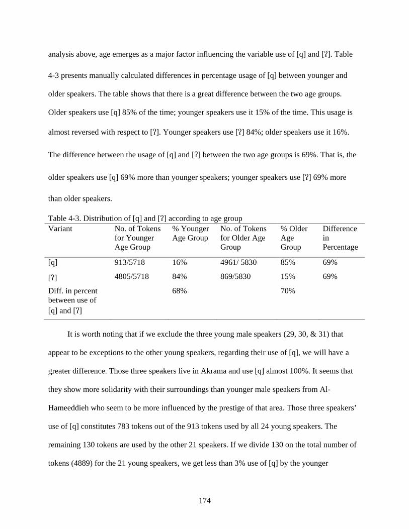
174
analysis above, age emerges as a major factor influencing the variable use of [q] and []. Table
4-3 presents manually calculated differences in percentage usage of [q] between younger and
older speakers. The table shows that there is a great difference between the two age groups.
Older speakers use [q] 85% of the time; younger speakers use it 15% of the time. This usage is
almost reversed with respect to []. Younger speakers use [] 84%; older speakers use it 16%.
The difference between the usage of [q] and [] between the two age groups is 69%. That is, the
older speakers use [q] 69% more than younger speakers; younger speakers use [] 69% more
than older speakers.
Table 4-3. Distribution of [q] and [] according to age group Variant No. of Tokens
for Younger Age Group
% Younger Age Group
No. of Tokens for Older Age Group
% Older Age Group
Difference in Percentage
[q] 913/5718 16% 4961/ 5830 85% 69%
[] 4805/5718 84% 869/5830 15% 69%
Diff. in percent between use of [q] and []
68% 70%
It is worth noting that if we exclude the three young male speakers (29, 30, & 31) that
appear to be exceptions to the other young speakers, regarding their use of [q], we will have a
greater difference. Those three speakers live in Akrama and use [q] almost 100%. It seems that
they show more solidarity with their surroundings than younger male speakers from Al-
Hameeddieh who seem to be more influenced by the prestige of that area. Those three speakers’
use of [q] constitutes 783 tokens out of the 913 tokens used by all 24 young speakers. The
remaining 130 tokens are used by the other 21 speakers. If we divide 130 on the total number of
tokens (4889) for the 21 young speakers, we get less than 3% use of [q] by the younger
175
generation. Calculating also the three speakers’ use of [] leads to a total of 46 tokens out of the
4805 tokens of the 24 speakers. Subtracting these 46 tokens from 4805 and dividing the resulting
number (4759) on the total number of tokens for the 21 young speakers (4889) gives a 97% use
of [] by the younger speakers.
These findings have a number of implications. First, the great difference between the two
age groups indicates that the shift towards the urban, prestigious form is quick. The younger
generation is more inclined towards the new form than older speakers. It took only one
generation to adopt the new form. Although the younger generation, in this study, are the sons
and daughters of the older generation and have been exposed to their parents’ linguistic forms
from birth, they show complete shift of linguistic interest. This situation is comparable to
Miller’s (2005:924) study of migrant speakers to Cairo. She suggests that the contact situation in
Cairo leads “to a long-term accommodation for the first migrant generation and to total
accommodation or dialect shift for the second generation, for example, those born in Cairo who
speak almost dominantly CA.” It seems that the younger speakers’ exposure to schools, which
involves mixing with native Himsi children, at an early age, has greatly influenced their choice
of a variant. In this sense, they started understanding the social stigma associated with [q] at an
earlier stage and were able to evade it by completely adopting the Himsi form, []. The city
social values along with their influence on the selection of a linguistic variant became their
values, leading to their selection of [] over [q]. This is the core of Mufwene’s (2005) theory of
language evolution and selection. Selection is very much influenced by the species’ surroundings
and their relationship to their environment. Adopting the social values of their surroundings leads
to restructuring of their parents’ initial input to adapt to their environment, an environment that
could be demanding linguistically and socially.
176
Second, some parents may be showing a struggle with this stigma, particularly older
females who show greater variation than older males. They are trying to adopt the new form.
Intra- and inter-speaker variation results from such attempts. Not all older speakers adopt the
prestigious form to the same degree. Such variation may be very indicative of a number of
issues. Older speakers are aware of the social stigma associated with [q], but they are unable to
employ their social knowledge to its fullest. Some of them show almost complete acquisition of
the new form (e.g., Speakers 17 & 21). Others do not show any kind of adaptation to the new
form. There are also those who oscillate between the two forms within the same conversation
with the same interlocutor. In the latter case, speakers probably have an internal struggle between
their original social values and the present social values that impose pressure on their linguistic
behavior. This internal struggle among social values leads to linguistic struggle because the
social and linguistic are highly associated. Those who do not show any adaptation to the new
environment could be the result of a fully developed social system that is very difficult to
interfere with after full development. This is similar to species that may easily change genetically
at their early stage of development for the sake of environmental adaptation, but once developed,
they hardly change.
This brings us to the third point. These findings are consonant with my theoretical proposal
in Chapter 3, in that, social factors should be treated on a continuous scale. They may be
employed completely in the adoption process, resulting in 100% usage of the new form. In other
words, their ranking values have been acquired and applied accurately in speech. In varying
speakers, their new ranking values are not totally acquired; hence, the observed oscillation
between the two forms. Speakers who do not show any kind of adoption of the new form seem to
cling to their original social values, and thus, the ranking values of their native form. Such
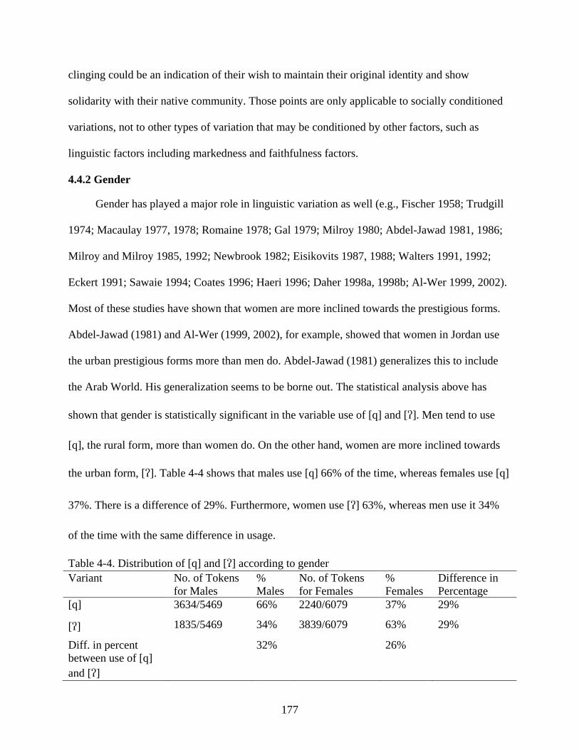
177
clinging could be an indication of their wish to maintain their original identity and show
solidarity with their native community. Those points are only applicable to socially conditioned
variations, not to other types of variation that may be conditioned by other factors, such as
linguistic factors including markedness and faithfulness factors.
4.4.2 Gender
Gender has played a major role in linguistic variation as well (e.g., Fischer 1958; Trudgill
1974; Macaulay 1977, 1978; Romaine 1978; Gal 1979; Milroy 1980; Abdel-Jawad 1981, 1986;
Milroy and Milroy 1985, 1992; Newbrook 1982; Eisikovits 1987, 1988; Walters 1991, 1992;
Eckert 1991; Sawaie 1994; Coates 1996; Haeri 1996; Daher 1998a, 1998b; Al-Wer 1999, 2002).
Most of these studies have shown that women are more inclined towards the prestigious forms.
Abdel-Jawad (1981) and Al-Wer (1999, 2002), for example, showed that women in Jordan use
the urban prestigious forms more than men do. Abdel-Jawad (1981) generalizes this to include
the Arab World. His generalization seems to be borne out. The statistical analysis above has
shown that gender is statistically significant in the variable use of [q] and []. Men tend to use
[q], the rural form, more than women do. On the other hand, women are more inclined towards
the urban form, []. Table 4-4 shows that males use [q] 66% of the time, whereas females use [q]
37%. There is a difference of 29%. Furthermore, women use [] 63%, whereas men use it 34%
of the time with the same difference in usage.
Table 4-4. Distribution of [q] and [] according to gender Variant No. of Tokens
for Males % Males
No. of Tokens for Females
% Females
Difference in Percentage
[q] 3634/5469 66% 2240/6079 37% 29%
[] 1835/5469 34% 3839/6079 63% 29%
Diff. in percent between use of [q] and []
32% 26%
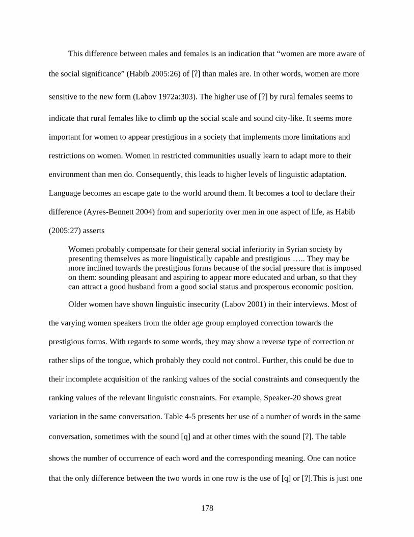
178
This difference between males and females is an indication that “women are more aware of
the social significance” (Habib 2005:26) of [] than males are. In other words, women are more
sensitive to the new form (Labov 1972a:303). The higher use of [] by rural females seems to
indicate that rural females like to climb up the social scale and sound city-like. It seems more
important for women to appear prestigious in a society that implements more limitations and
restrictions on women. Women in restricted communities usually learn to adapt more to their
environment than men do. Consequently, this leads to higher levels of linguistic adaptation.
Language becomes an escape gate to the world around them. It becomes a tool to declare their
difference (Ayres-Bennett 2004) from and superiority over men in one aspect of life, as Habib
(2005:27) asserts
Women probably compensate for their general social inferiority in Syrian society by presenting themselves as more linguistically capable and prestigious ….. They may be more inclined towards the prestigious forms because of the social pressure that is imposed on them: sounding pleasant and aspiring to appear more educated and urban, so that they can attract a good husband from a good social status and prosperous economic position.
Older women have shown linguistic insecurity (Labov 2001) in their interviews. Most of
the varying women speakers from the older age group employed correction towards the
prestigious forms. With regards to some words, they may show a reverse type of correction or
rather slips of the tongue, which probably they could not control. Further, this could be due to
their incomplete acquisition of the ranking values of the social constraints and consequently the
ranking values of the relevant linguistic constraints. For example, Speaker-20 shows great
variation in the same conversation. Table 4-5 presents her use of a number of words in the same
conversation, sometimes with the sound [q] and at other times with the sound []. The table
shows the number of occurrence of each word and the corresponding meaning. One can notice
that the only difference between the two words in one row is the use of [q] or [].This is just one
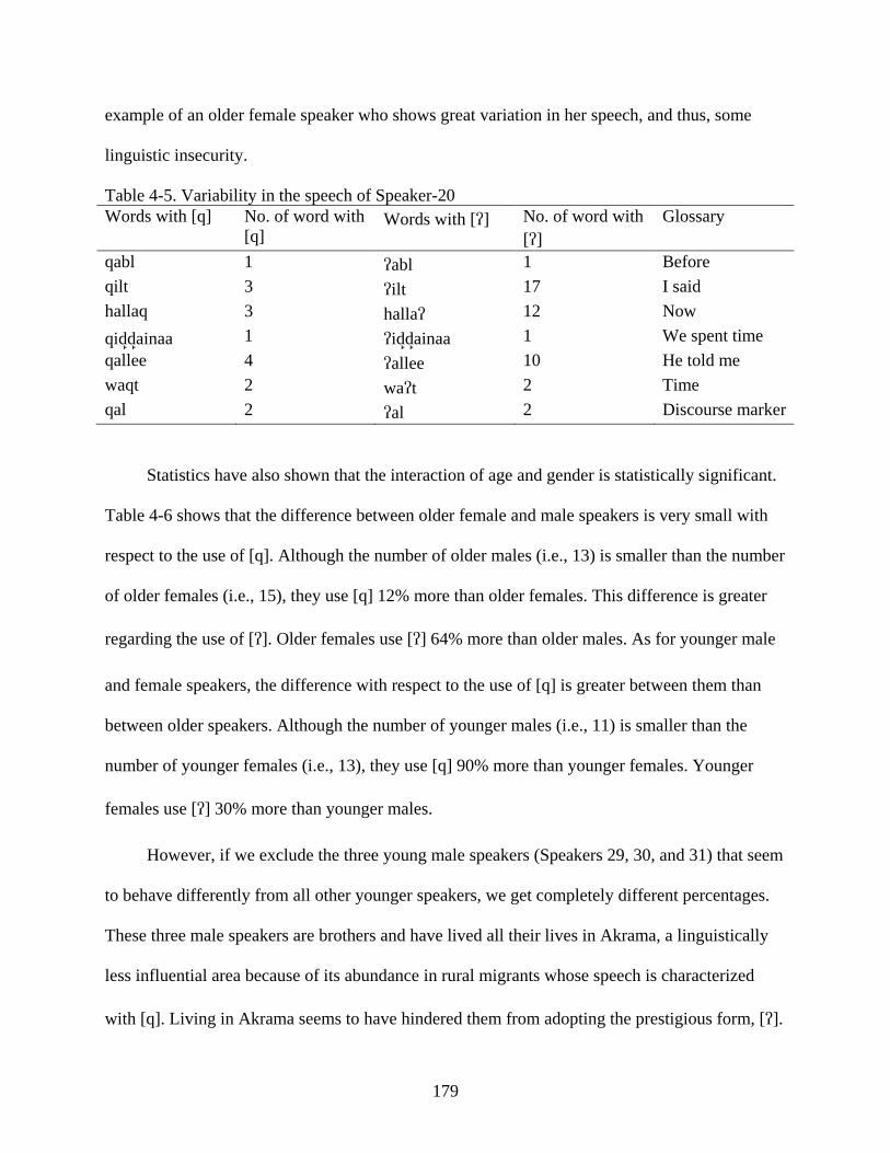
179
example of an older female speaker who shows great variation in her speech, and thus, some
linguistic insecurity.
Table 4-5. Variability in the speech of Speaker-20 Words with [q] No. of word with
[q] Words with [] No. of word with
[] Glossary
qabl 1 abl 1 Before qilt 3 ilt 17 I said hallaq 3 halla 12 Now qiddainaa 1 iddainaa 1 We spent time qallee 4 allee 10 He told me waqt 2 wat 2 Time qal 2 al 2 Discourse marker
Statistics have also shown that the interaction of age and gender is statistically significant.
Table 4-6 shows that the difference between older female and male speakers is very small with
respect to the use of [q]. Although the number of older males (i.e., 13) is smaller than the number
of older females (i.e., 15), they use [q] 12% more than older females. This difference is greater
regarding the use of []. Older females use [] 64% more than older males. As for younger male
and female speakers, the difference with respect to the use of [q] is greater between them than
between older speakers. Although the number of younger males (i.e., 11) is smaller than the
number of younger females (i.e., 13), they use [q] 90% more than younger females. Younger
females use [] 30% more than younger males.
However, if we exclude the three young male speakers (Speakers 29, 30, and 31) that seem
to behave differently from all other younger speakers, we get completely different percentages.
These three male speakers are brothers and have lived all their lives in Akrama, a linguistically
less influential area because of its abundance in rural migrants whose speech is characterized
with [q]. Living in Akrama seems to have hindered them from adopting the prestigious form, [].
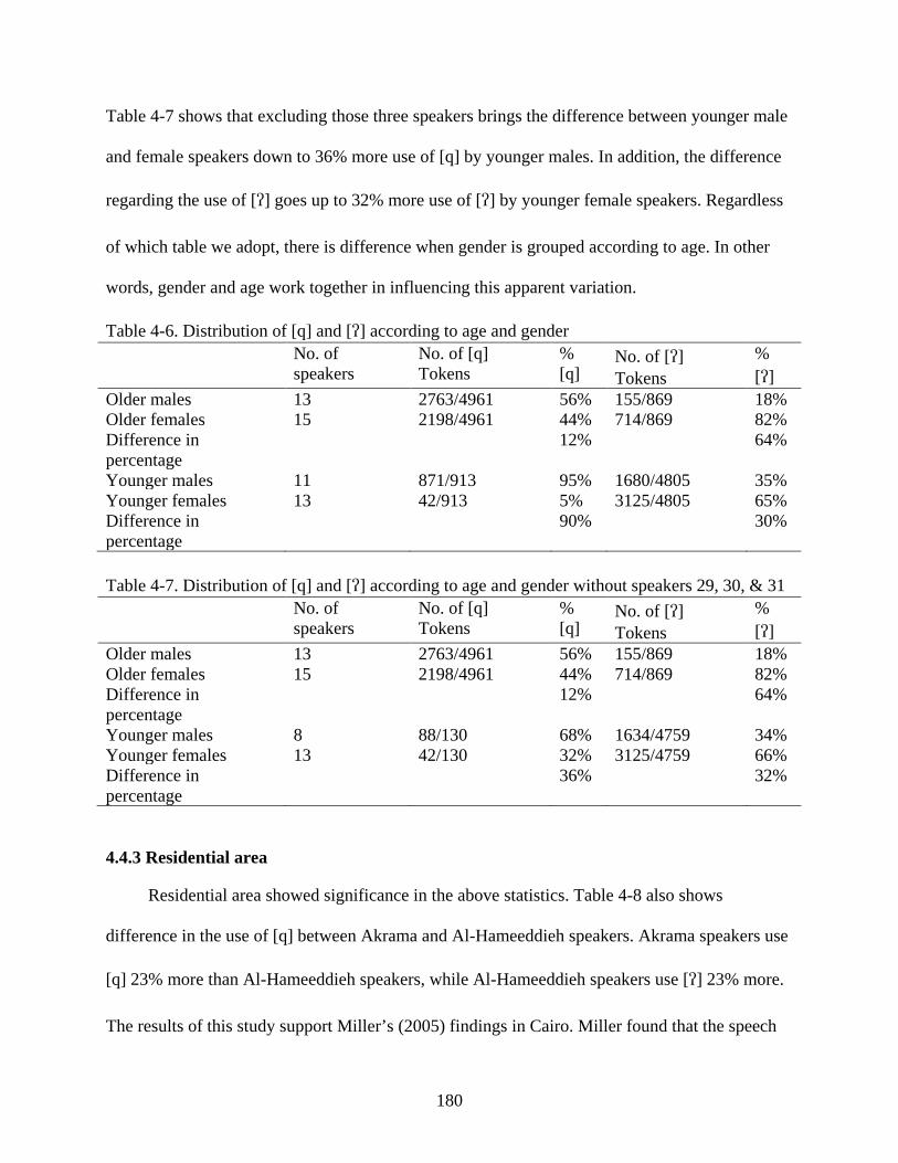
180
Table 4-7 shows that excluding those three speakers brings the difference between younger male
and female speakers down to 36% more use of [q] by younger males. In addition, the difference
regarding the use of [] goes up to 32% more use of [] by younger female speakers. Regardless
of which table we adopt, there is difference when gender is grouped according to age. In other
words, gender and age work together in influencing this apparent variation.
Table 4-6. Distribution of [q] and [] according to age and gender No. of
speakers No. of [q] Tokens
% [q]
No. of [] Tokens
% []
Older males 13 2763/4961 56% 155/869 18% Older females 15 2198/4961 44% 714/869 82% Difference in percentage
12% 64%
Younger males 11 871/913 95% 1680/4805 35% Younger females 13 42/913 5% 3125/4805 65% Difference in percentage
90% 30%
Table 4-7. Distribution of [q] and [] according to age and gender without speakers 29, 30, & 31 No. of
speakers No. of [q] Tokens
% [q]
No. of [] Tokens
% []
Older males 13 2763/4961 56% 155/869 18% Older females 15 2198/4961 44% 714/869 82% Difference in percentage
12% 64%
Younger males 8 88/130 68% 1634/4759 34% Younger females 13 42/130 32% 3125/4759 66% Difference in percentage
36% 32%
4.4.3 Residential area
Residential area showed significance in the above statistics. Table 4-8 also shows
difference in the use of [q] between Akrama and Al-Hameeddieh speakers. Akrama speakers use
[q] 23% more than Al-Hameeddieh speakers, while Al-Hameeddieh speakers use [] 23% more.
The results of this study support Miller’s (2005) findings in Cairo. Miller found that the speech
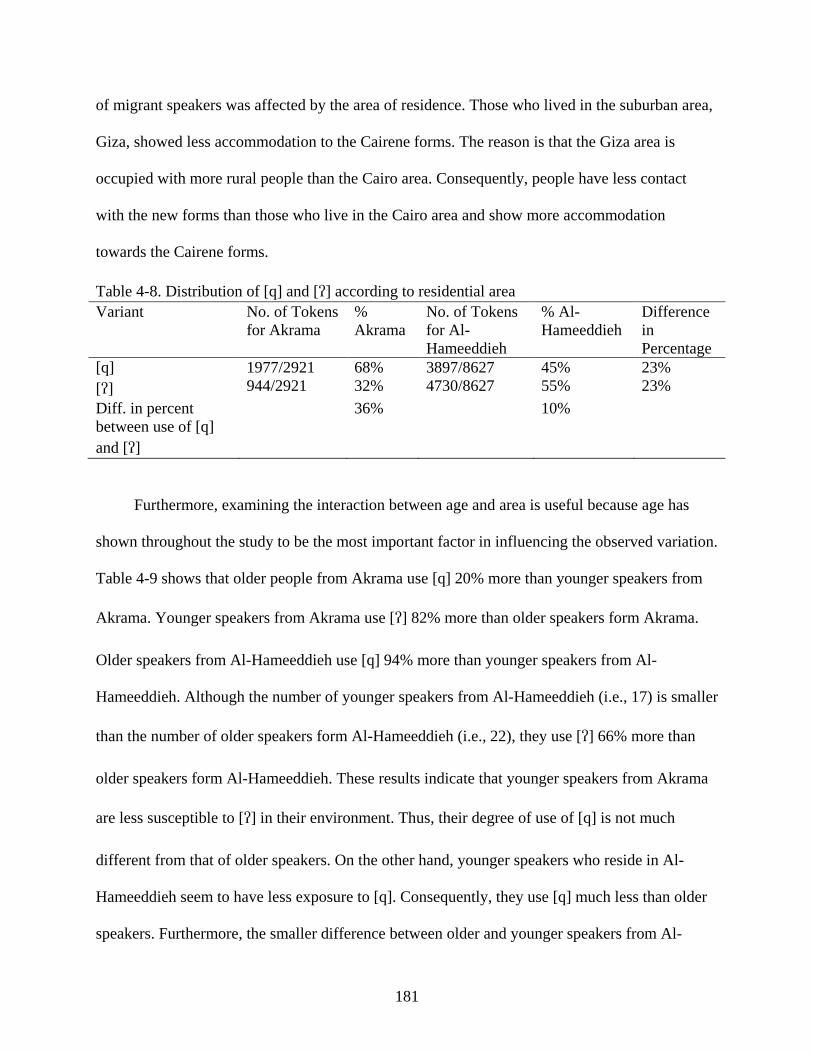
181
of migrant speakers was affected by the area of residence. Those who lived in the suburban area,
Giza, showed less accommodation to the Cairene forms. The reason is that the Giza area is
occupied with more rural people than the Cairo area. Consequently, people have less contact
with the new forms than those who live in the Cairo area and show more accommodation
towards the Cairene forms.
Table 4-8. Distribution of [q] and [] according to residential area Variant No. of Tokens
for Akrama % Akrama
No. of Tokens for Al-Hameeddieh
% Al-Hameeddieh
Difference in Percentage
[q] 1977/2921 68% 3897/8627 45% 23% [] 944/2921 32% 4730/8627 55% 23% Diff. in percent between use of [q] and []
36% 10%
Furthermore, examining the interaction between age and area is useful because age has
shown throughout the study to be the most important factor in influencing the observed variation.
Table 4-9 shows that older people from Akrama use [q] 20% more than younger speakers from
Akrama. Younger speakers from Akrama use [] 82% more than older speakers form Akrama.
Older speakers from Al-Hameeddieh use [q] 94% more than younger speakers from Al-
Hameeddieh. Although the number of younger speakers from Al-Hameeddieh (i.e., 17) is smaller
than the number of older speakers form Al-Hameeddieh (i.e., 22), they use [] 66% more than
older speakers form Al-Hameeddieh. These results indicate that younger speakers from Akrama
are less susceptible to [] in their environment. Thus, their degree of use of [q] is not much
different from that of older speakers. On the other hand, younger speakers who reside in Al-
Hameeddieh seem to have less exposure to [q]. Consequently, they use [q] much less than older
speakers. Furthermore, the smaller difference between older and younger speakers from Al-
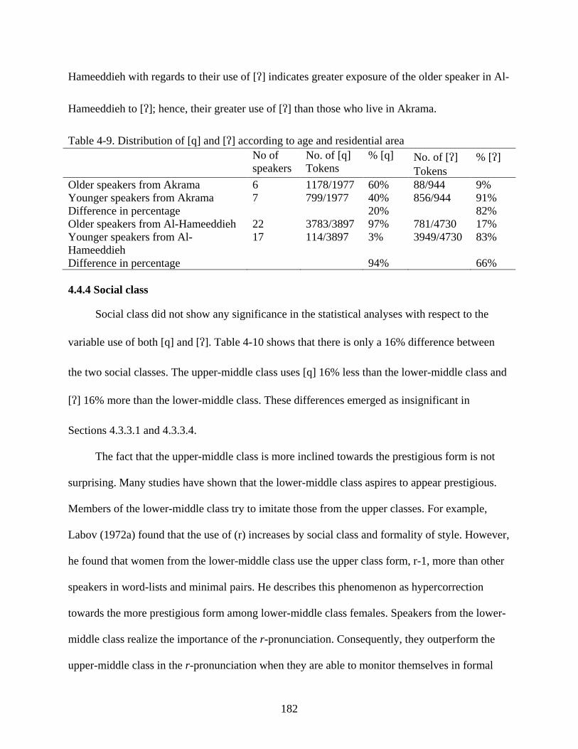
182
Hameeddieh with regards to their use of [] indicates greater exposure of the older speaker in Al-
Hameeddieh to []; hence, their greater use of [] than those who live in Akrama.
Table 4-9. Distribution of [q] and [] according to age and residential area No of
speakers No. of [q] Tokens
% [q] No. of [] Tokens
% []
Older speakers from Akrama 6 1178/1977 60% 88/944 9% Younger speakers from Akrama 7 799/1977 40% 856/944 91% Difference in percentage 20% 82% Older speakers from Al-Hameeddieh 22 3783/3897 97% 781/4730 17% Younger speakers from Al-Hameeddieh
17 114/3897 3% 3949/4730 83%
Difference in percentage 94% 66% 4.4.4 Social class
Social class did not show any significance in the statistical analyses with respect to the
variable use of both [q] and []. Table 4-10 shows that there is only a 16% difference between
the two social classes. The upper-middle class uses [q] 16% less than the lower-middle class and
[] 16% more than the lower-middle class. These differences emerged as insignificant in
Sections 4.3.3.1 and 4.3.3.4.
The fact that the upper-middle class is more inclined towards the prestigious form is not
surprising. Many studies have shown that the lower-middle class aspires to appear prestigious.
Members of the lower-middle class try to imitate those from the upper classes. For example,
Labov (1972a) found that the use of (r) increases by social class and formality of style. However,
he found that women from the lower-middle class use the upper class form, r-1, more than other
speakers in word-lists and minimal pairs. He describes this phenomenon as hypercorrection
towards the more prestigious form among lower-middle class females. Speakers from the lower-
middle class realize the importance of the r-pronunciation. Consequently, they outperform the
upper-middle class in the r-pronunciation when they are able to monitor themselves in formal

183
styles, such as reading word-lists or minimal pairs. This phenomenon is also termed as the
“crossover pattern” (Labov 1972a) or “apparent deviation” (Labov 1966:227). Such crossover
patterns are taken as a sign for change in progress. Like Labov (1966, 1972a), Trudgill (1974)
found a crossover pattern in the use of the variable (ing) in Norwich. Female speakers from the
lower-middle class showed a great shift from the use of -in in casual style to the use of -ing in
formal style. This shift is much greater in the lower-middle class than it is in any other social
group. However, in other studies like Milroy’s (1980), males from working classes showed less
use of the prestigious form in Belfast because of their strong connection to their working class
community. It is a way of expressing solidarity with their fellow workers.
Table 4-10. Distribution of [q] and [] according to social class Variant No. of Tokens
for LM % LM
No. of Tokens for UM
% UM
Difference in Percentage
[q] 3655/6284 58% 2219/5264 42% 16 [] 2629/6284 42% 3045/5264 58% 16 Diff. in percent between use of [q] and []
16% 16%
Since social class emerged as statistically insignificant, the associated factors such as
income and occupation are assumed, in Section 4.2, not to play a role on their own, by
inheritance, in determining variation in the use of [q] and []. A GZLM procedure was
performed to examine the influence of income, occupation, and education on each of the variants
[q] and []. The results are included in Appendix E. The results show that income (p = 0.318),
occupation (p = 0.804), and education (p = 0.353) do not play a significant role in the variable
use of [q]. However, the results are slightly different with respect to the variable use of [].
Income (p = 0.114) and occupation (p = 0.148), which are associated with social class, do not
184
play a significant role. In contrast, Education, which is not associated with social class, plays a
significant role (p = 0.000). Speakers with elementary education [Education = 1] (p = 0.531) and
middle-school education [Education = 2] do not show significance according to the Parameter
Estimates Table. The other four educational categories show significance. The least significant
category is speakers with high-school education [Education = 3] (p = 0.043). The other three
categories – associate degree [Education = 4], bachelor’s degree [Education = 5], and
professional [Education = 6] – are highly significant, all of which have the p–value (p = 0.000).
Examining the coefficients in the Parameter Estimates Table, we notice that the higher the
education, the higher the use of []. The coefficient for professional [Education = 6] is 4.029,
indicating that professionals use [] much more than other categories. The Exp(B) is 56.201,
which informs us that the odds that professionals will use the [] sound is 56 times the odds that
other educational categories will use the [].The coefficient for bachelor’s degree [Education =
5] is 3.588, indicating that speakers with a bachelor’s degree use [] much more than those with
less education. The Exp(B) is 36.169, which informs us that the odds that speakers with a
bachelor’s degree will use the [] sound is 36 times the odds that lower educational categories
will use the []. The coefficient for associate degree [Education = 4] is 3.473, indicating that
speakers with an associate degree use [] much more than those with less education. The Exp(B)
is 32.249, which informs us that the odds that speakers with an associate degree will use the []
sound is 32 times the odds that lower educational categories will use the []. The coefficient for
high school [Education = 3] is 1.836, indicating that speakers with high school education use []
more than those with less education. The Exp(B) is 6.274, which informs that the odds that
185
speakers with high school education will use the [] sound is 6 times the odds that speakers with
middle school or elementary school education will use the [].
These findings implicate that schooling greatly affects a speaker’s adoption of the
prestigious form, []. Although in formal education the [q] sound is the basis for learning reading
and writing (Daher 1998a; Haeri 2003), it seems that the social influence of the people we
interact with in the school setting is greater, resulting in increased use of [] and decreased use of
[q]. This finding is very interesting because it emphasizes the need to separate, in the Arab
World, between what is considered prestigious in speech, [] in our case, and what is prestigious
or standard in formal education, [q]. This separation was first suggested by Ibrahim (1986:125)
“Standard Arabic has a certain degree of prestige and its religious, ideological, and educational
values are undeniable, but its social evaluative connotations are much weaker than those of
locally prestigious varieties.” Walters (1996:177), likewise, differentiates between two norms, a
norm that is chosen for “free speech” and is “local”, the other is chosen for reading aloud and is
“external”. Hachimi (2001:30) further refers to the possibility of having “competing prestige
varieties”. Thus, even local varieties may carry different types of prestige and may be evaluated
differently by different speakers based on the social class they belong to or their educational and
occupational background.
4.4.5 Relationship of the Statistical Findings to the Theoretical Analysis
In Chapter 3, I showed that the three social constraints *F[], *OLD[], and *AKR[] are
involved in giving us results that match real life occurrences of [q] (82%) and [] (18%) in the
speech of older female speakers from Akrama. The quantitative analysis of this chapter has
shown that there is significant interaction between gender, age, and residential area with respect
186
to the use of [q], not with respect to the use of []. This finding slightly contradicts with the
findings of the theoretical analysis. Although, it reveals that there is interaction among the three
factors, it eliminates this interaction in the case of the variable use of []. Consequently, the
theoretical analysis has an advantage over the quantitative analysis, in that it shows that there is
partial interaction among the three factors with regards to the variable use of each of the
independent variants. The theoretical analysis splits each social factor into four different
constrains and specifies exactly which of the four constraints is involved. In this sense, only one
of the constraints may be involved at one time or used by a certain speaker or group of speakers,
whose effect may not show clearly in the quantitative analysis. Furthermore, not all speakers
may use the same social factor in the same way. Speakers may activate different constraints
within the same social factor. For example, I showed that younger female speakers from Al-
Hameeddieh activate *F[q], *YOUNG[q], and *HAM[q], as opposed to older female speakers
from Akrama, to arrive at their real life occurrences of [q] (2%) and [] (98%). These results tell
us that residential area interacts with age and gender with regards to the use of [], in contrast to
the results of the quantitative analysis. This finding highlights one further advantage of the
theoretical analysis. Although a whole factor may not be involved in the interaction with regards
to the use of one variant, part of it may be implemented by some speakers. Thus, the theoretical
proposal of this study allows for more options and accounts more closely for the differences
among different groups of speakers as well as individual speakers, which is very hard to do in
one step in the statistical analyses. The theoretical analysis shows that it is not sufficient to say
that this factor does not interact with other factors. It informs us specifically what constraint(s)
is(are) involved. It also gives us the mental representation of how these factors interact with the
linguistic constraints and how they influence the ranking values of those constraints.
187
Furthermore, the theoretical proposal allows us to see that certain social constraints may have
higher ranking values in some speakers than others. For examples, we have seen that *M[] may
have a higher ranking value than *F[] in the speech of older male speakers from Akrama
because of their higher use of [q] (96%) and lower use of [] (4%) than older female speakers
from Akrama. This is a further advantage of the theoretical analysis. It can indicate that one
social factor, such as gender, may be more important to one group of speakers than another
group of speakers. In the case of the variable use of [q] and [], it may explain the masculine
connotation of [q] and the feminine connotation of [] in the literature (Sawaie 1994; Daher
1998a). Moreover, it may explain the masculine meaning that is associated with non-prestigious
forms versus the feminine meaning associated with the prestigious forms (Abdel-Jawad 1986).
Nonetheless, the quantitative analysis cannot be disregarded completely because it has also
its advantages, such as giving us a head start on what social factors may be involved or not,
particularly for someone who may not be very familiar with the community. For someone who is
from a community under investigation, like me, s/he will be able in the theoretical analysis to
know the social constraints that are involved in the learning process for each group of speakers.
Knowing the gender, area, and age of the speaker and the linguistic behavior of that speaker or
group of speakers would enable a researcher to easily discover the social constraints involved in
the speech of that speaker. Furthermore, I have mentioned in Chapter 3 that the GLA gives
predications on what the speech of speakers would sound like if certain social constraints are
involved. A listener is also capable of discovering the social constraints employed by a certain
speaker at a certain time and place because they are familiar with their environment and the
social constraints that are usually activated by different speakers. The GLA also gives
188
representations of the amount of input of each variant that a speaker or a group of speakers is
exposed to. Thus, it reflects on the social networks of the speakers. It can tell us that those older
female speakers from Akrama receive approximately 82% input of [q] and 18% input of [],
implicating that the Akrama environment is more dense with rural people and it is not a good
environment for acquiring the new form quickly. This is apparent in the speech of the three
young male speakers from Akrama (29, 30, & 31). They differ from their counterparts who
reside in Al-Hameeddieh and who only took one generation to acquire the new form completely.
The complete acquisition of [] by young female speakers from Al-Hameeddieh is a further
indication of the density of Himsi people in that area and that Al-Hameeddieh is a facilitative
learning environment of the new form.
This discussion leaves us with one further question. How does the learning process
proceeds? In other words, do speakers learn some words quicker than others? If that is the case,
does the frequency of certain words influence such acquisition? We have seen that the variable
use of [q] and [] is influenced by social factors. However, it is worth examining if this variation
proceeds first in the direction of the most common words than it does in the direction of the less
frequent words.
4.5 Frequency Effects on the Acquisition of []
It is expected that highly frequent words will be acquired faster by speakers than less
frequent words (Pierrehumbert 2001; Medoza-Denton, Hay, & Jannedy 2003). First, I entered the
words for each speaker in a separate table, grouping similar words together. Then, I created one
huge table in which I grouped similar words from all speakers. I added the number of similar
words to examine the frequency of their occurrence. I extracted from that huge table the most
frequent words produced with [], words that occur 20 times or more (Table 4-11). I also
189
extracted the most frequent words produced with [q], words that occur 20 times or more (Table
4-11). I performed this extraction because it may help in making comparison between the two
lists – the [] list and the [q] list. Having similar words in the two frequent lists may be a further
indication that the frequency of these words leads to faster acquisition of them. The frequency of
words produced with [q] does not necessary mean that it will negatively affect the acquisition.
Rather, it informs us that those words are very frequent in speech in society in general and that
people are exposed to them more often than to other words.
The process of learnability of the new form [] will be noticed significantly if we examine
the words produced with [] by older speakers whose speech is characterized with variation. For
this reason, I decided to investigate the words used with the [] sound by those speakers. The
speakers who show greater variability are speakers 5, 6, 9, 16, 19, 20, 23, 25, and 28. There are
older speakers who show minor variability, such as speakers 1, 3, 8, 11, and 22. I will examine
first those with lower variability and then those with higher variability to see which words with
the [] sound are used by them. Then, I will present in Table 4-12, the number of occurrence of
some of the frequent words extracted in Table 4-11 in their speech in comparison to less frequent
words. I will also calculate the percentage of the occurrence of these frequent words in relation
to other words uttered with [] in their speech to arrive at conclusions regarding whether
frequency has influenced their acquisition of certain words before other words.
Table 4-12 strongly suggests that the more frequent the word, the more likely to occur in
the speech of varying speakers. This implies that frequently occurring words are acquired faster
than non-frequent words. In most of the varying speakers the word halla ‘now’ shows the
highest percentages because it is the most frequent word in Table 4-11 (735 tokens with [] and
190
457 tokens with [q]). Even in speakers whose variation is minor, this word seems to penetrate
into their system because of its high frequency, as is the case with regards to speakers 1, 3, 8, and
11 (Table 4-12). The second most frequent word in Table 4-11 is wat ‘time’ (295 occurrences
with []). Table 4-12 shows that this word occurs in high percentages in the speech of most
speakers. For example, it is the only occurring word besides halla ‘now’ in the speech of
Speaker-8 and has a higher percentage than halla ‘now’ (Table 4-12). It has the highest
percentage after halla ‘now’ in the speech of Speaker-16 (Table 4-12). The next four words in
frequency are aal ‘said’, ilt ‘I/you said’, baaa ‘so/such/yet’, and allee ‘he told me’ (264,
234, 124, , and 115 occurrences with [] respectively) (Table 4-11). aal ‘said’, for instance, has
the second highest percentage in Speaker-25, the third highest percentage in Speakers 16 & 19 ,
and the fourth highest percentage in Speaker-20 (Table 4-12). It occurs in the speech of most
other speakers. ilt ‘I/you said’ has the second highest percentage in Speakers 19 & 28. It also
occurs in the speech of most other speakers. baaa ‘so/such/yet’ has the second highest
percentage in Speaker-23, the third highest percentage in Speaker-28, the fourth highest
percentage in Speakers 6 & 16, and the fifth highest percentage in Speakers 9 & 25. This word
appears in the speech of most other speakers. allee ‘he told me’ has the third highest percentage
in Speaker-20 and it occurs in the speech of most other speakers. It is worth noting here that a
word like allee ‘he told me’ is related semantically to other frequently occurring words like
allaa ‘he told her’, alluu ‘he told him’, uul ‘say/I say’, etc. All of these words carry the
semantic meaning of ‘saying’. They are calculated independently from each other. However, it is
possible to group them together because they are derived from the same root in Arabic. Arabic
191
morphology depends mainly on root and patterns; patterns are added to roots to derive other
words which are semantically related. Grouping them together will give higher frequencies of
them. Although the various forms of this verb and other words have been calculated separately, I
do not eliminate the possibility that speakers may operate on the basis of the frequency of the
root, not the word. Feldman, Frost, and Pnini (1995) have argued that morphemes and rules are
stored in the brain, comparing English, a concatenative language, with Hebrew, a non-
concatenative language like Arabic. Their study showed morphological relatedness effects in a
repetition priming study among words that share the same root, even at long lags. This indicates
that roots are stored separately in the lexicon and are accessed quickly by speakers who have
encountered them earlier on in speech. Once accessed, speakers apply stored rules to build or
decipher semantically related words. Nonetheless, Beret, Vaknin, and Marcus (2006) argued that
in Hebrew, stems, not roots, are stored in the brain, although their findings do not completely
eliminate the possibility of roots being stored. On the other hand, Davis and Zawaydeh (2001)
and Arad (2003) propose that both stems and roots are stored in the brain. This point is beyond
the scope of this study and requires further research.
In conclusion, from comparisons between Table 4-11 and Table 4-12, one can confirm that
frequency plays a major role in the acquisition process. Mostly, high frequency words are the
ones that occur in the speech of varying speakers. This is apparent in the high percentages of
these words in their speech. We have seen that the more frequent the word, the higher its
percentage in the speech of varying speakers. This leads to the conclusion that the more frequent
the word, the faster the acquisition of that word and the more likely for it to be acquired by
learners. Highly frequent words are even acquired by those whose speech can be characterized
with almost 100% use of [q]. Knowing the frequency of a word allows us to make predications
192
on whether this word is used by varying speakers or not. In other words, the frequency of words
gives expectations on what a varying speaker’s speech is likely to contain. Moreover, frequency
should not be understood as the main reason for acquisition of the new form. Social factors
impose pressure on speakers to adopt the new form. The role of frequency is leading this
adoption process towards the most common words first.
4.6 Conclusion
This chapter has shown the influence of social factors on the variable use of [q] and [].
The results have shown that age, gender, and residential area play major roles in affecting this
variation. Social class emerged as an insignificant factor in this variation. The results have also
shown some interaction between the three significant factors with respect to the use of [q], but
not with regards to the use of []. The interaction between gender and age proved significant for
both variants. The chapter has also tested the association between social class and education,
income, occupation, and residential area. Education did not show significant association with
social class. Income and residential area showed the most significance. Occupation proved to be
significant with respect to the government employees’ category. The factors that showed
association with social class, occupation and income, did not have an effect on the variable use
of [q] and []. However, education showed some significance with respect to the use of []
independently from social class, to which it is not associated. The chapter has also shown some
advantages of the theoretical analysis over the quantitative analysis. The theoretical analysis
allows more specificity with regards to social factors; it gives clearer picture of what revolves in
the mind of a speaker at a certain time and place. While some social constraints within one social
factor may be activated by a speaker or a group of speaker, they may not be activated by others.
While the quantitative analysis did not show interaction among age, gender, and residential area
193
with regards to the use of [], the theoretical analysis was able to show this interaction because of
its specificity. Furthermore, the theoretical analysis has shown that one social constraint within
one social factor may have a higher ranking value within the same speech community than its
counterpart. This specificity is not as achievable in the quantitative analysis as it is in the
theoretical analysis. Finally, this chapter has shown that word frequency influence the acquisition
process. Highly frequent words are acquired before less frequent words. The following chapter
will present a quantitative analysis of the four variants [t] and [s] and [d] and [z]. Those four
variants will be dealt with differently from the two variants [q] and [] because as we have seen
they are not socially conditioned.

194
Table 4-11. Most frequent words produced with [q] and [] Word produced
with [] No. of tokens
Matching word produced with [q]
Glossary No. of tokens
1 halla/halle 735 hallaq/halleq Now 457 2 wat 295 waqt Time 82 3 aal 264 qaal Said 424 4 ilt 234 qilt I/you said 397 5 baaa 124 baqaa So/such/yet 98 6 allee 115 qallee He told me 172 7 abl 96 qabl Before 87 8 aam 77 qaam Discourse marker (Lit. ‘got
up/did’) 41
9 rifaat/rifeet 76 rifqaat Friends 53 10 uulee 68 quulee You can say/say 61 11 a 58 aqq Right/price 49 12 tlaaee 52 tlaaqee You can find 22 13 rfii 50 rfiiq Friend 24 14 illik 50 qillik I tell you 110 15 biiuuloo 49 quuloo You (pl)/they say 47 16 addee 42 qaddee How much 19 17 t arii 42 t ariiq Road/way 48 18 tariiban/tariiban 43 taqriiban/taqriiben Almost/approximately 59 19 alluu 41 qalluu He told him 148 20 far 38 farq Difference 13 21 al 36 qal Discourse marker (Lit. ‘it has
been said’) 139
22 aad 36 qaad He sat/lived 7 23 is s a 35 qis s a Story 21 24 imt/umit 34 qimt Discourse marker (Lit. ‘I got
up/did’) 3
25 add 33 qadd As much 34 26 allaa 32 qallaa He told her 42 27 alb 32 qalb Heart 39 28 uul 31 quul Say/I say 20 29 aadi 31 qaadi/deedi Sitting/living (F) 10 30 foo 31 fooq Up/above/upstairs 55 31 ilnaa 30 qilnaa We said 88 32 iddaam/iddeem 31 qiddaam/qiddeem Before/in front of 60
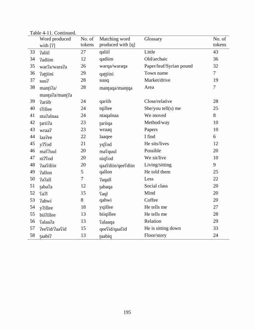
195
Table 4-11. Continued. Word produced
with [] No. of tokens
Matching word produced with [q]
Glossary No. of tokens
33 aliil 27 qaliil Little 43 34 adiim 12 qadiim Old/archaic 36 35 wara/waraa 26 warqa/waraqa Paper/leaf/Syrian pound 32 36 at tiini 29 qat tiini Town name 7 37 suu 28 suuq Market/drive 19 38 mant ia/
mant aa/mant a 28 mant aqa/mant qa Area 7
39 ariib 24 qariib Close/relative 28 40 tillee 24 tqillee She/you tell(s) me 25 41 ntaalnaa 24 ntaqalnaa We moved 8 42 t ariia 23 t ariiqa Method/way 10 43 wraa 23 wraaq Papers 10 44 laaee 22 laaqee I find 6 45 yod 21 yqod He sits/lives 12 46 mauul 20 maquul Possible 20 47 niod 20 niqod We sit/live 10 48 aadiin 20 qaadiin/qeediin Living/sitting 9 49 allon 5 qallon He told them 25 50 aall 7 aqall Less 22 51 t abaa 12 t abaqa Social class 20 52 al 15 aql Mind 20 53 ahwi 8 qahwi Coffee 20 54 yillee 18 yqillee He tells me 27 55 biiillee 13 biiqillee He tells me 28 56 alaaa 13 alaaqa Relation 29 57 eeid/aaid 15 qeeid/qaaid He is sitting down 33 58 t aabi 13 t aabiq Floor/story 24
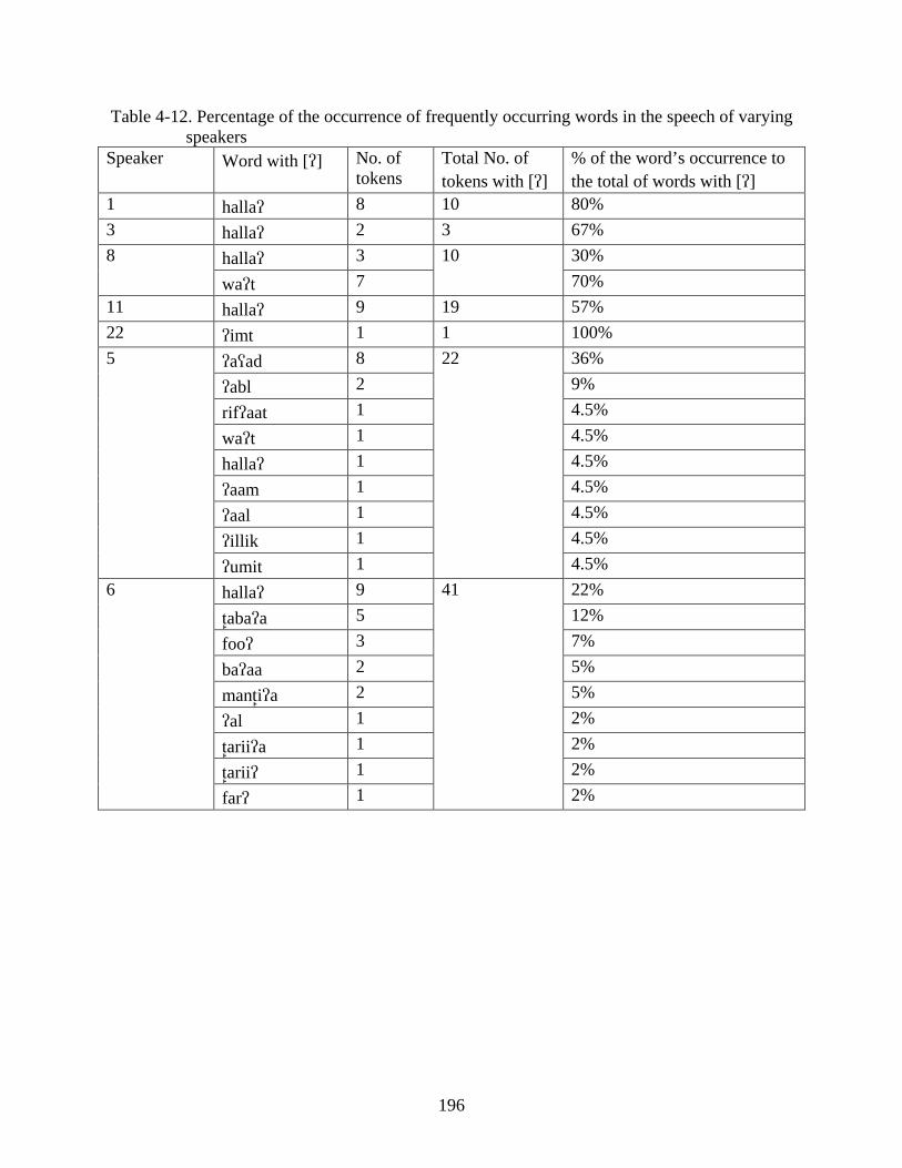
196
Table 4-12. Percentage of the occurrence of frequently occurring words in the speech of varying speakers
Speaker Word with [] No. of tokens
Total No. of tokens with []
% of the word’s occurrence to the total of words with []
1 halla 8 10 80% 3 halla 2 3 67% 8 halla 3 10 30%
wat 7 70% 11 halla 9 19 57% 22 imt 1 1 100% 5 aad 8 22 36%
abl 2 9% rifaat 1 4.5% wat 1 4.5% halla 1 4.5% aam 1 4.5% aal 1 4.5% illik 1 4.5% umit 1 4.5%
6 halla 9 41 22% t abaa 5 12% foo 3 7% baaa 2 5% mant ia 2 5% al 1 2% t ariia 1 2% t arii 1 2% far 1 2%
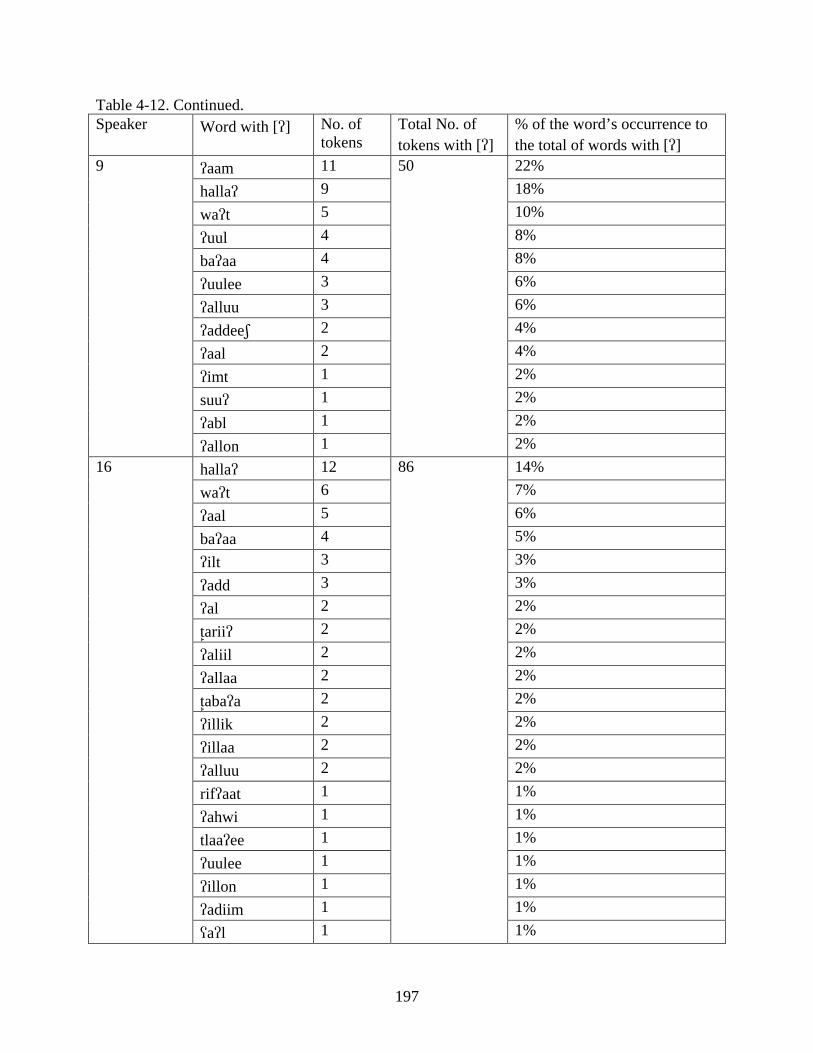
197
Table 4-12. Continued. Speaker Word with [] No. of
tokens Total No. of tokens with []
% of the word’s occurrence to the total of words with []
9 aam 11 50 22% halla 9 18% wat 5 10% uul 4 8% baaa 4 8% uulee 3 6% alluu 3 6% addee 2 4% aal 2 4% imt 1 2% suu 1 2% abl 1 2% allon 1 2%
16 halla 12 86 14% wat 6 7% aal 5 6% baaa 4 5% ilt 3 3% add 3 3% al 2 2% t arii 2 2% aliil 2 2% allaa 2 2% t abaa 2 2% illik 2 2% illaa 2 2% alluu 2 2% rifaat 1 1% ahwi 1 1% tlaaee 1 1% uulee 1 1% illon 1 1% adiim 1 1% al 1 1%
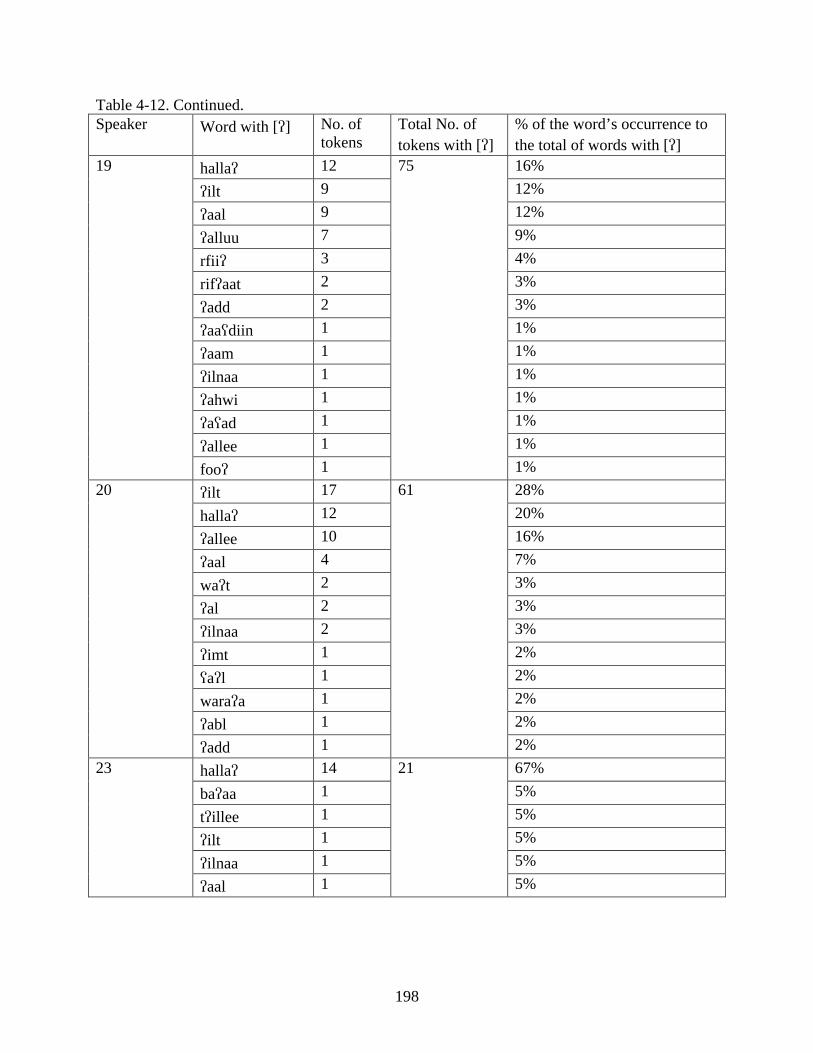
198
Table 4-12. Continued. Speaker Word with [] No. of
tokens Total No. of tokens with []
% of the word’s occurrence to the total of words with []
19 halla 12 75 16% ilt 9 12% aal 9 12% alluu 7 9% rfii 3 4% rifaat 2 3% add 2 3% aadiin 1 1% aam 1 1% ilnaa 1 1% ahwi 1 1% aad 1 1% allee 1 1% foo 1 1%
20 ilt 17 61 28% halla 12 20% allee 10 16% aal 4 7% wat 2 3% al 2 3% ilnaa 2 3% imt 1 2% al 1 2% waraa 1 2% abl 1 2% add 1 2%
23 halla 14 21 67% baaa 1 5% tillee 1 5% ilt 1 5% ilnaa 1 5% aal 1 5%
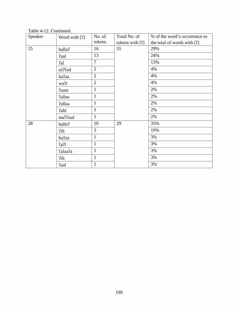
199
Table 4-12. Continued. Speaker Word with [] No. of
tokens Total No. of tokens with []
% of the word’s occurrence to the total of words with []
25 halla 16 55 29% aal 13 24% al 7 13% niod 2 4% baaa 2 4% wat 2 4% aam 1 2% allee 1 2% allaa 1 2% abl 1 2% mauul 1 2%
28 halle 10 29 35% ilt 3 10% baaa 1 3% al 1 3% alaaa 1 3% ilt 1 3% aal 1 3%
200
CHAPTER 5 QUANTITATIVE ANALYSIS OF THE VARIANTS [t] AND [s] AND [d] AND [z]
5.1 Introduction
Because all speakers behave in the same way regarding the use of the variants [t] and [s]
and [d] and [z], social factors do not seem to play a role in this type of variation. If social factors
were to play a role, we would notice variation among speakers and groups of speakers. On the
contrary, what we notice is that certain words are always used by all speakers with only one of
the variants, [t] or [s] or [d] or [z]. In Chapter 3, I have shown that the linguistic environment
does not influence the use of one variant over another. This led me to examine the frequency of
these words to see if the number of occurrences of words has diachronically led to the present
stable phenomenon.
To investigate the effect of frequency on the use of the four variants, I entered the words
pronounced with each of the four variants in a separate table for each speaker, grouping similar
words together. Then, I grouped similar words from all speakers in one large table to arrive at the
frequency of each word in the speech of all 52 speakers. Then, I summarized the most frequent
words in Tables 5-1 and 5-6. The results of this process will be explored in the following
sections. I will first start with the frequency analysis of the two sounds [t] and [s] followed by a
discussion of the results. Then, I will present the frequency analysis of the two sounds [d] and [z]
followed by a discussion of the results. The general discussion and conclusion Sections 5.6 and
5.7 will touch on usage-based theory proposed by Bybee (2001) and on how this theory is able to
explain the present situation as a result of two different diachronic changes.
5.2 Analysis of the Use of [t] and [s]
I extracted from the large table, in which I grouped all similar words produced with [t] and
[s] and [d] and [z] together, the most frequent words produced with [t] and [s], words whose
201
frequency is 10 or higher (Table 5-1). The total number of words produced with [t] is 2767.
Table 5-1 shows that the most frequent word produced with [t] is ktiir ‘much/a lot’; it occurs
1159 times, which constitutes 42% of the total number of words produced with [t]. The second
most frequent word is mitl ‘like/as’ (288 tokens = 10%). The third word in frequency is
aktar/aktor15 ‘more’ (245 tokens = 9%). tlat ‘three’ (153 tokens), taanee/teenee ‘second (M)’
(149 tokens), and tlaati ‘three’ (123 tokens) are respectively next highest in frequency. They
constitute 6%, 5%, and 4% of the total number of words produced with [t] respectively. Though
tlat and tlaati have exactly the same meaning, their syntactic position is usually different, and
thus their usage. tlat is used as the first term of a construct state (two consecutive nouns) (e.g.,
tlat kutub ‘three books’). It cannot stand as a number on its own or be connected to an enclitic
pronoun. tlaati, on the other hand, is used as a number on its own and can be suffixed to an
enclitic pronoun (e.g., tlaatiton ‘the three of them’). Other words such as tlaatiin/tleetiin ‘thirty’
(93 tokens = 3%), tneen ‘two’ (71 tokens = 3%) and taaniiyii/teeniiyii ‘second (F)’ (64 tokens =
2%) also show high frequency.
As for the variant [s], the total number of words produced with [s] is 870. The most
frequent word produced with [s] is masalin/masalan ‘for example/instance’ (530 tokens = 61%).
This seems to be the most frequent word among all words produced with [s]. Other words such
as saair ‘a proper noun’ (19 tokens), adiis ‘modern/talk’ (18 tokens), and aadis ‘accident’
(16 tokens) constitute about 2% each.
15 aktar occurs in free variation with aktor. aktar is the HCA; aktor is the RCA from. This example shows one of the vowel differences between the two dialects. As aktor and aktar occur in free variation, other subsequent words in the text such as taanee/teenee, tlaatiin/tleetiin, taaniiyii/teeniiyii, masalan/masalin occur in free variation. In each of these pairs of words, the first term is the HCA form; the second term is the RCA form. These are examples that show vowel differences between the two dialects. RCA speakers who reside in Hims may vary their speech regarding the use of these vowels, which is beyond the scope of this study.
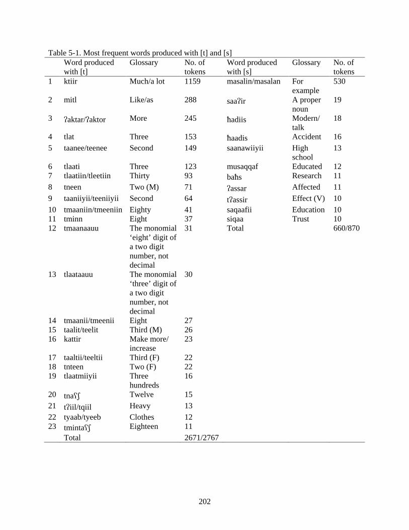
202
Table 5-1. Most frequent words produced with [t] and [s] Word produced
with [t] Glossary No. of
tokens Word produced with [s]
Glossary No. of tokens
1 ktiir Much/a lot 1159 masalin/masalan For example
530
2 mitl Like/as 288 saair A proper noun
19
3 aktar/aktor More 245 adiis Modern/ talk
18
4 tlat Three 153 aadis Accident 16 5 taanee/teenee Second 149 saanawiiyii High
school 13
6 tlaati Three 123 musaqqaf Educated 12 7 tlaatiin/tleetiin Thirty 93 bas Research 11 8 tneen Two (M) 71 assar Affected 11 9 taaniiyii/teeniiyii Second 64 tassir Effect (V) 10 10 tmaaniin/tmeeniin Eighty 41 saqaafii Education 10 11 tminn Eight 37 siqaa Trust 10 12 tmaanaauu The monomial
‘eight’ digit of a two digit number, not decimal
31 Total 660/870
13 tlaataauu The monomial ‘three’ digit of a two digit number, not decimal
30
14 tmaanii/tmeenii Eight 27 15 taalit/teelit Third (M) 26 16 kattir Make more/
increase 23
17 taaltii/teeltii Third (F) 22 18 tnteen Two (F) 22 19 tlaatmiiyii Three
hundreds 16
20 tna Twelve 15 21 tiil/tqiil Heavy 13 22 tyaab/tyeeb Clothes 12 23 tminta Eighteen 11 Total 2671/2767
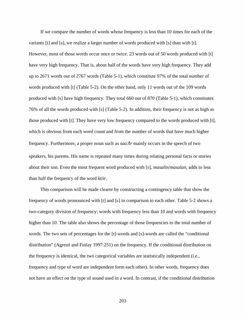
203
If we compare the number of words whose frequency is less than 10 times for each of the
variants [t] and [s], we realize a larger number of words produced with [s] than with [t].
However, most of those words occur once or twice. 23 words out of 50 words produced with [t]
have very high frequency. That is, about half of the words have very high frequency. They add
up to 2671 words out of 2767 words (Table 5-1), which constitute 97% of the total number of
words produced with [t] (Table 5-2). On the other hand, only 11 words out of the 109 words
produced with [s] have high frequency. They total 660 out of 870 (Table 5-1), which constitutes
76% of all the words produced with [s] (Table 5-2). In addition, their frequency is not as high as
those produced with [t]. They have very low frequency compared to the words produced with [t],
which is obvious from each word count and from the number of words that have much higher
frequency. Furthermore, a proper noun such as saair mainly occurs in the speech of two
speakers, his parents. His name is repeated many times during relating personal facts or stories
about their son. Even the most frequent word produced with [s], masalin/masalan, adds to less
than half the frequency of the word ktiir.
This comparison will be made clearer by constructing a contingency table that show the
frequency of words pronounced with [t] and [s] in comparison to each other. Table 5-2 shows a
two-category division of frequency: words with frequency less than 10 and words with frequency
higher than 10. The table also shows the percentage of those frequencies to the total number of
words. The two sets of percentages for the [t]-words and [s]-words are called the “conditional
distribution” (Agresti and Finlay 1997:251) on the frequency. If the conditional distribution on
the frequency is identical, the two categorical variables are statistically independent (i.e.,
frequency and type of word are independent form each other). In other words, frequency does
not have an effect on the type of sound used in a word. In contrast, if the conditional distribution
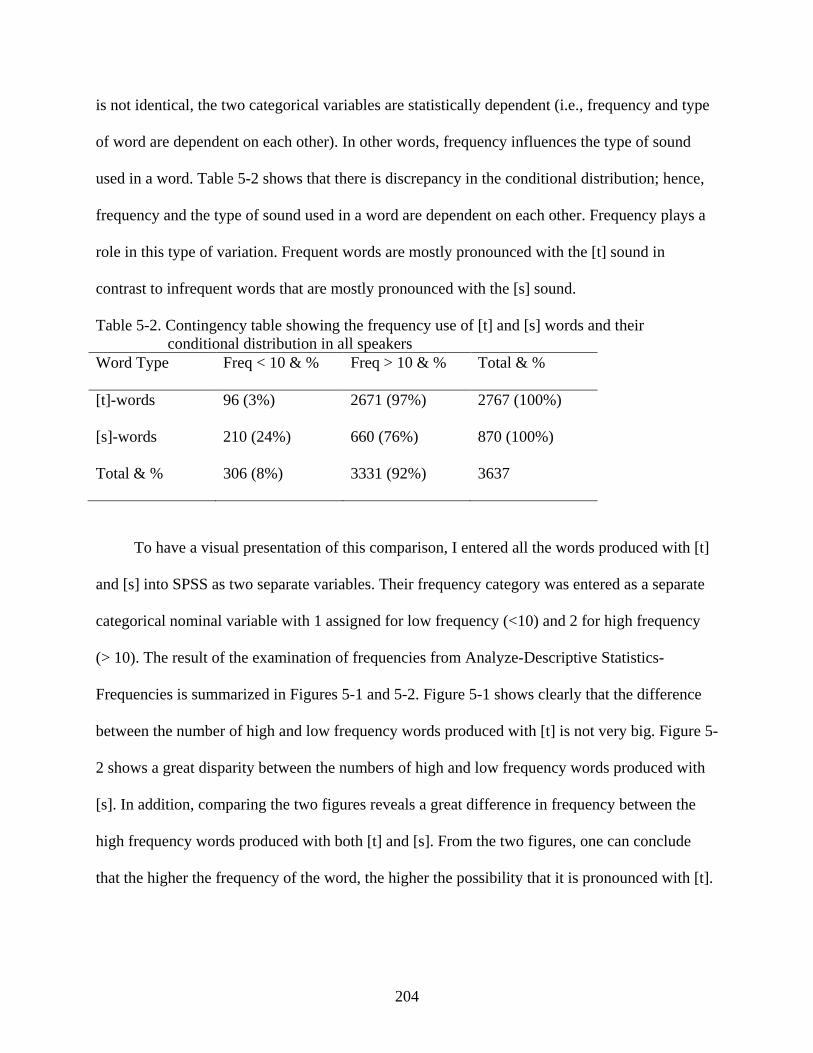
204
is not identical, the two categorical variables are statistically dependent (i.e., frequency and type
of word are dependent on each other). In other words, frequency influences the type of sound
used in a word. Table 5-2 shows that there is discrepancy in the conditional distribution; hence,
frequency and the type of sound used in a word are dependent on each other. Frequency plays a
role in this type of variation. Frequent words are mostly pronounced with the [t] sound in
contrast to infrequent words that are mostly pronounced with the [s] sound.
Table 5-2. Contingency table showing the frequency use of [t] and [s] words and their conditional distribution in all speakers
Word Type Freq < 10 & % Freq > 10 & % Total & %
[t]-words 96 (3%) 2671 (97%) 2767 (100%)
[s]-words 210 (24%) 660 (76%) 870 (100%)
Total & % 306 (8%) 3331 (92%) 3637
To have a visual presentation of this comparison, I entered all the words produced with [t]
and [s] into SPSS as two separate variables. Their frequency category was entered as a separate
categorical nominal variable with 1 assigned for low frequency (<10) and 2 for high frequency
(> 10). The result of the examination of frequencies from Analyze-Descriptive Statistics-
Frequencies is summarized in Figures 5-1 and 5-2. Figure 5-1 shows clearly that the difference
between the number of high and low frequency words produced with [t] is not very big. Figure 5-
2 shows a great disparity between the numbers of high and low frequency words produced with
[s]. In addition, comparing the two figures reveals a great difference in frequency between the
high frequency words produced with both [t] and [s]. From the two figures, one can conclude
that the higher the frequency of the word, the higher the possibility that it is pronounced with [t].
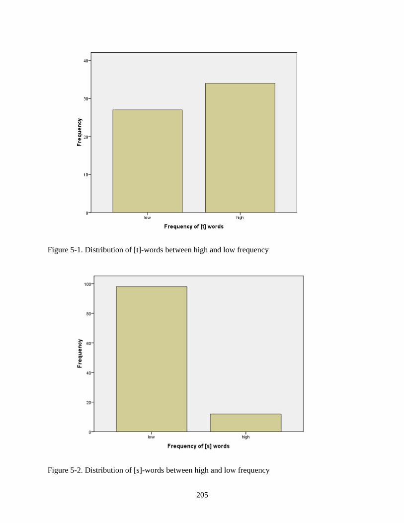
205
Figure 5-1. Distribution of [t]-words between high and low frequency
Figure 5-2. Distribution of [s]-words between high and low frequency
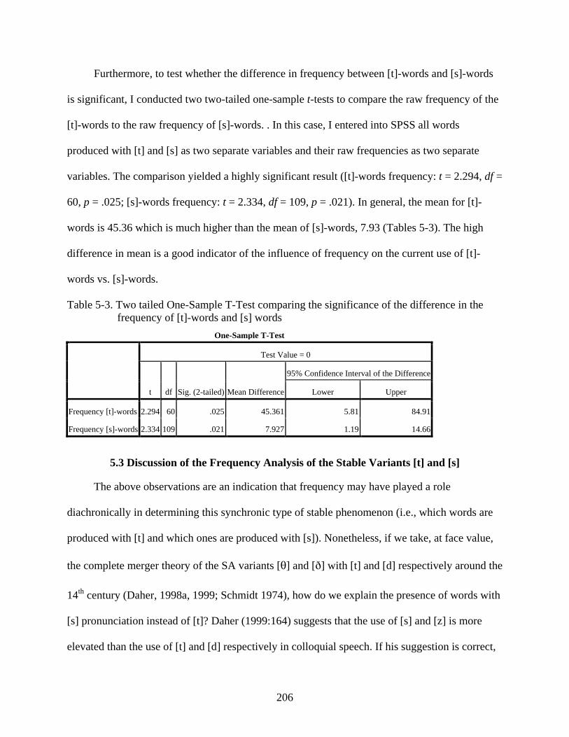
206
Furthermore, to test whether the difference in frequency between [t]-words and [s]-words
is significant, I conducted two two-tailed one-sample t-tests to compare the raw frequency of the
[t]-words to the raw frequency of [s]-words. . In this case, I entered into SPSS all words
produced with [t] and [s] as two separate variables and their raw frequencies as two separate
variables. The comparison yielded a highly significant result ([t]-words frequency: t = 2.294, df =
60, p = .025; [s]-words frequency: t = 2.334, df = 109, p = .021). In general, the mean for [t]-
words is 45.36 which is much higher than the mean of [s]-words, 7.93 (Tables 5-3). The high
difference in mean is a good indicator of the influence of frequency on the current use of [t]-
words vs. [s]-words.
Table 5-3. Two tailed One-Sample T-Test comparing the significance of the difference in the frequency of [t]-words and [s] words
One-Sample T-Test
Test Value = 0
t df Sig. (2-tailed) Mean Difference
95% Confidence Interval of the Difference
Lower Upper
Frequency [t]-words 2.294 60 .025 45.361 5.81 84.91
Frequency [s]-words 2.334 109 .021 7.927 1.19 14.66
5.3 Discussion of the Frequency Analysis of the Stable Variants [t] and [s]
The above observations are an indication that frequency may have played a role
diachronically in determining this synchronic type of stable phenomenon (i.e., which words are
produced with [t] and which ones are produced with [s]). Nonetheless, if we take, at face value,
the complete merger theory of the SA variants [] and [] with [t] and [d] respectively around the
14th century (Daher, 1998a, 1999; Schmidt 1974), how do we explain the presence of words with
[s] pronunciation instead of [t]? Daher (1999:164) suggests that the use of [s] and [z] is more
elevated than the use of [t] and [d] respectively in colloquial speech. If his suggestion is correct,
207
we would expect variation among speakers and groups of speakers. This is not the case in my
data. All speakers behave similarly. According to some studies, a second change occured some
time after the 14th century (Birkeland 1952; Schmidt 1986:57; Schulz 1981:33; all cited in Daher
1999). Borrowed words form SA with the [] and [] variants were replaced in colloquial speech
with [s] and [z] respectively. This seems plausible given the following observations.
The non-frequent words with the [t] sound are related semantically to the frequent words.
They are derived from the same root and most of them are related to the numbers three and eight
as well as the word for much. On the other hand, the low frequency words with the sound [s] are
not necessarily semantically related to those of high frequency, but they may be semantically
related to each other. A close examination of these words reveals that many of them have the
vowel system of the SA corresponding words, indicating that they are mainly borrowings from
SA. However, due to the high markedness of the sound [], the sound [s] is used instead. Table
5-4 presents just a few examples that show the similarity in vowel system between the observed
forms and their SA corresponding forms. Other words may have shown some assimilation to the
vowel system of the dialects, but this change is less likely to happen word-internally. It mostly
occurs word-finally as a result of suffixing a colloquial suffix in place of the SA suffix, for
example, the colloquial feminine marker [-i] in place of the SA feminine marker [-a] (Examples
1-3 in Table 5-5); the relational adjective marker [-ee] in place of [-iiy] (Examples 4 & 5 in
Table 5-5); or a colloquial pronominal in place of a SA pronominal (Examples 6 & 7 in Table 5-
5). There is a number of word-internal vowel assimilation to the vowel system of the dialects, as
in Examples 8 & 9 in Table 5-5. The integration of the SA root with the colloquial dialects
patterns could be an indication that roots and patterns are stored separately in the brain because
speakers could interlock the root of the SA with a pattern from the colloquial dialects. Thus, the

208
root is borrowed from SA, not the pattern, in some cases. Furthermore, the previously observed
semantic relatedness among words that are produced with one of the two variants provides
evidence for the possibility that roots and patterns are stored separately in the brain, because
roots are “semantic abstractions” from which semantically related words are derived (Holes
2004:99). Speakers seem to use the same root with its dialectal phonemic representation (i.e., the
same sound [t] or [s]) in different words that are semantically related.
Table 5-4. Similarity between the vowel system of observed words with [s] with their counterparts in SA
Observed word with [s] SA corresponding word with [] Glossary 1 asar aar Trace 2 asnaa anaa During 3 isbaat ibaat Proof 4 adaas adaa Incidents 5 saabit aabit Firm/fixed 6 tamsiil tamiil Acting Table 5-5. Assimilated words with [s] to the vowel system of the dialects Observed word with [s] SA corresponding word with [] Glossary 1 wiraas-i wiraa-a Heredity/ inheritance 2 basi ba-a Delegation 3 lissi li-a Gum 4 sawaanee awaan-iiy Seconds 5 saanawee aanaw-iiy High school 6 saqaaft-uu aqaafatu-huu His education 7 ytadds-oo yataadda-uuna They talk 8 tuusaq-ee taiq-iina You (F) trust 9 tuuras tari Inherit
In Chapter 3, I have established that /t/ and /s/ are the underlying form for [t] and [s]
respectively in colloquial speech. The phonological representations of these two sounds are
accessed when using similar words. Because phonemes constitute morphemes and roots are
separate morphemes in Arabic, one can conclude that speakers access these root morphemes with
209
their phonemic representations. The status of the root and the pattern in the brain is beyond the
scope of this study and requires further research. They are mentioned here to show that there is
the possibility that some words (more specifically roots/morphemes) are borrowed from SA and
are intersected with colloquial morphology and phonology. The borrowings show assimilation to
the vowel system of the dialects and adoption of the phonemic system of those dialects, which
consists of the phonemes /t/ and /s/, not //.
5.4 Analysis of the Use of [d] and [z]
I also extracted from the large table that contains all words produced with [t] and [s] and
[d] and [z] the most frequent words produced with [d] and [z], words whose frequency is 10 or
higher (Table 5-6). The total number of tokens produced with [d] is 1740. Table 5-6 shows that
the most frequent word produced with [d] is haadaa ‘this (M)’; it occurs 607 times, which
constitutes 35% of the total number of words produced with [d]. The second most frequent word
is hadool ‘these’ (135 tokens = 8%). The third word in frequency is haadii ‘this (F)’ (116 tokens
= 7%). aad ‘took’ (114 tokens = 7%), hadiik ‘that (F)’ (67 tokens = 4%), and ad ‘take’ (59
tokens = 3%) are respectively next highest in frequency. Other words such as aaod ‘I take’ (48
tokens = 3%), yaaod ‘he takes’ (48 tokens = 3%) and aad ‘take’ (47 tokens = 3%) also show
high frequency. It is also worth noting here that there are a number of variants of haadaa ‘this
(M)’, hadool ‘these’, and haadii ‘this (F)’, all pronounced with [d], but they show various vowel
patterns. These words are haad ‘this (M)’ (2 tokens), hadaa ‘this (M)’ (1 token), hedaa ‘this
(M)’ (1 token), hidaak ‘that (M)’ (1 token), hauud ‘these’ (1 token), hauudaalee ‘these’ (2
tokens), haduuk ‘those’ (4 tokens), and haidii ‘this (F)’ (8 tokens). If we add these words to their
respective variants (i.e., those with which they show free variation), we will find even higher
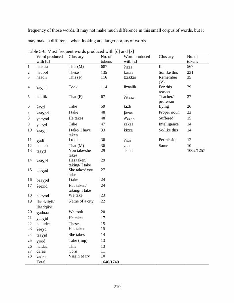
210
frequency of those words. It may not make much difference in this small corpus of words, but it
may make a difference when looking at a larger corpus of words.
Table 5-6. Most frequent words produced with [d] and [z] Word produced
with [d] Glossary No. of
tokens Word produced with [z]
Glossary No. of tokens
1 haadaa This (M) 607 izaa If 567 2 hadool These 135 kazaa So/like this 231 3 haadii This (F) 116 tzakkar Remember
(V) 35
4 aad Took 114 lizaalik For this reason
29
5 hadiik That (F) 67 staaz Teacher/ professor
27
6 ad Take 59 kizb Lying 26 7 aaod I take 48 azaa Proper noun 22 8 yaaod He takes 48 tzzab Suffered 15 9 yaad Take 47 zakaa Intelligence 14 10 aad I take/ I have
taken 33 kizza So/like this 14
11 adt I took 30 izn Permission 12 12 hadaak That (M) 30 zaat Same 10 13 taad You take/she
takes 29 Total 1002/1257
14 aaid Has taken/ taking/ I take
29
15 taaod She takes/ you take
27
16 baaod I take 24 17 eexid Has taken/
taking/ I take 24
18 naaod We take 23 19 llaadiiyii/
llaadqiiyii Name of a city 22
20 adnaa We took 20 21 yaaid He takes 17 22 hauudee These 15 23 eed Has taken 15 24 taaid She takes 14 25 ood Take (imp) 13 26 haidaa This 13 27 daraa Corn 11 28 adraa Virgin Mary 10 Total 1640/1740
211
As for the variant [z], the total number of tokens produced with [z] is 1257 (Table 5-6).
The most frequent word produced with [z] is izaa ‘if’ (567 tokens = 45%). The second most
frequent word is kazaa ‘so/like this’ (231 tokens = 18%). tzakkar ‘remember’ (35 tokens)
constitutes 3%. Other words such as lizaalik ‘for this reason’ (29 tokens), and staaz
‘teacher/Mr./professor’ (27 tokens), and kizb ‘lying’ (26 tokens) constitute about 2% each.
If we compare the number of words whose frequency is less than 10 times for each of the
variants [d] and [z], we realize a larger number of words produced with [z] than with [d].
However, most of those words occur once or twice. 28 words out of 64 words produced with [d]
have very high frequency. That is, about half of the words have very high frequency. They add
up to 1640 words out of 1740 words (Table 5-6), which constitute 94% of the total number of
words produced with [d] (Table 5-7). On the other hand, only 12 words out of the 138 words
produced with [z] have high frequency. They total 1002 out of 1257 (Table 5-6), which
constitutes 80% of all the words produced with [z] (Table 5-7). In addition, the frequency of
most of the words produced with [z] is not as high as those produced with [d]. Most of them have
very low frequency compared to the words produced with [d], which is obvious from each word
count and from the number of words that have higher frequency. However, two words produced
with [z] could be considered exceptions regarding their high frequency: izaa ‘if’ that occurs 567
times and kazaa ‘so/like this’ that occurs 231 times. I attribute the high frequency of these two
words to their being a conditional expression and a discourse marker respectively. Consequently,
these two words occur frequently in speech.
As in the case of words with [t] and [s], this comparison will be made clearer by
constructing a contingency table that show the frequency of words pronounced with [d] and [z]
in comparison to each other. Table 5-7 shows the two-category division of frequency and the
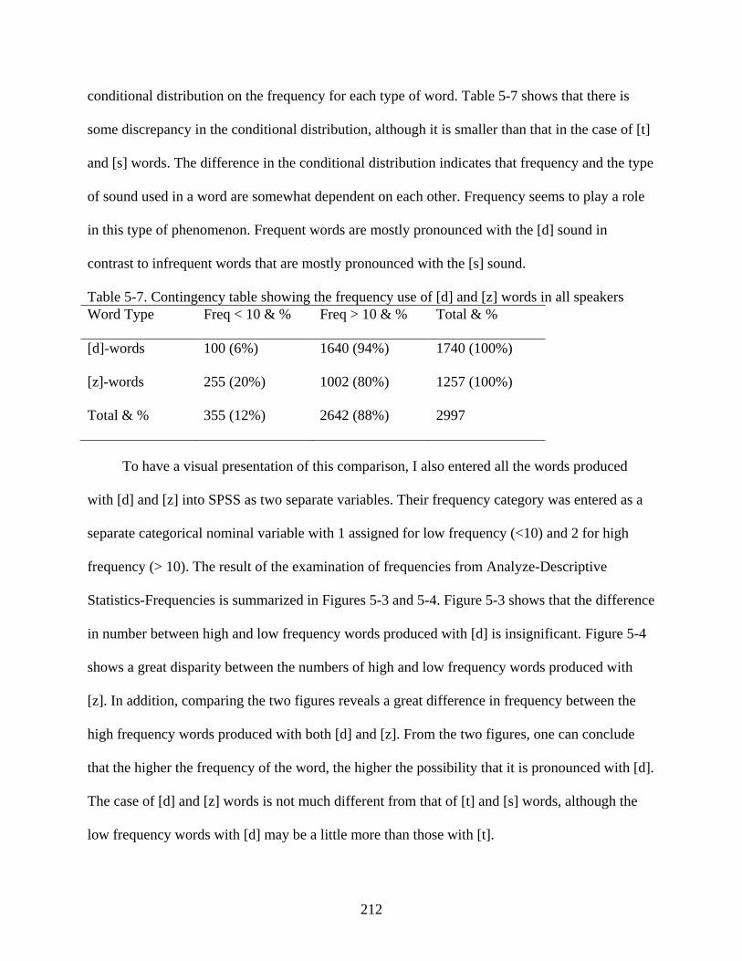
212
conditional distribution on the frequency for each type of word. Table 5-7 shows that there is
some discrepancy in the conditional distribution, although it is smaller than that in the case of [t]
and [s] words. The difference in the conditional distribution indicates that frequency and the type
of sound used in a word are somewhat dependent on each other. Frequency seems to play a role
in this type of phenomenon. Frequent words are mostly pronounced with the [d] sound in
contrast to infrequent words that are mostly pronounced with the [s] sound.
Table 5-7. Contingency table showing the frequency use of [d] and [z] words in all speakers Word Type Freq < 10 & % Freq > 10 & % Total & %
[d]-words 100 (6%) 1640 (94%) 1740 (100%)
[z]-words 255 (20%) 1002 (80%) 1257 (100%)
Total & % 355 (12%) 2642 (88%) 2997
To have a visual presentation of this comparison, I also entered all the words produced
with [d] and [z] into SPSS as two separate variables. Their frequency category was entered as a
separate categorical nominal variable with 1 assigned for low frequency (<10) and 2 for high
frequency (> 10). The result of the examination of frequencies from Analyze-Descriptive
Statistics-Frequencies is summarized in Figures 5-3 and 5-4. Figure 5-3 shows that the difference
in number between high and low frequency words produced with [d] is insignificant. Figure 5-4
shows a great disparity between the numbers of high and low frequency words produced with
[z]. In addition, comparing the two figures reveals a great difference in frequency between the
high frequency words produced with both [d] and [z]. From the two figures, one can conclude
that the higher the frequency of the word, the higher the possibility that it is pronounced with [d].
The case of [d] and [z] words is not much different from that of [t] and [s] words, although the
low frequency words with [d] may be a little more than those with [t].

213
Figure 5-3. The distribution of [d]-words between high and low frequency
Figure 5-4. The distribution of [z]-words between high and low frequency
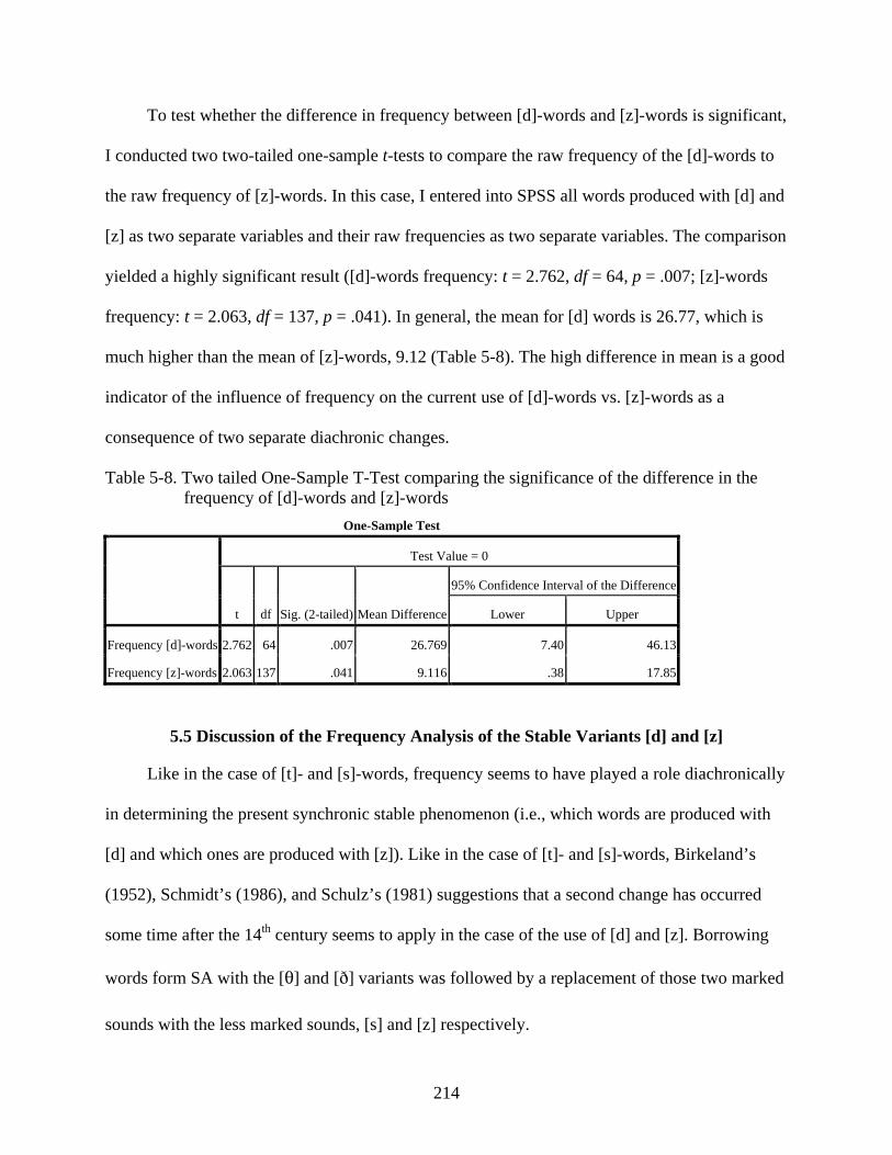
214
To test whether the difference in frequency between [d]-words and [z]-words is significant,
I conducted two two-tailed one-sample t-tests to compare the raw frequency of the [d]-words to
the raw frequency of [z]-words. In this case, I entered into SPSS all words produced with [d] and
[z] as two separate variables and their raw frequencies as two separate variables. The comparison
yielded a highly significant result ([d]-words frequency: t = 2.762, df = 64, p = .007; [z]-words
frequency: t = 2.063, df = 137, p = .041). In general, the mean for [d] words is 26.77, which is
much higher than the mean of [z]-words, 9.12 (Table 5-8). The high difference in mean is a good
indicator of the influence of frequency on the current use of [d]-words vs. [z]-words as a
consequence of two separate diachronic changes.
Table 5-8. Two tailed One-Sample T-Test comparing the significance of the difference in the frequency of [d]-words and [z]-words
One-Sample Test
Test Value = 0
t df Sig. (2-tailed) Mean Difference
95% Confidence Interval of the Difference
Lower Upper
Frequency [d]-words 2.762 64 .007 26.769 7.40 46.13
Frequency [z]-words 2.063 137 .041 9.116 .38 17.85
5.5 Discussion of the Frequency Analysis of the Stable Variants [d] and [z]
Like in the case of [t]- and [s]-words, frequency seems to have played a role diachronically
in determining the present synchronic stable phenomenon (i.e., which words are produced with
[d] and which ones are produced with [z]). Like in the case of [t]- and [s]-words, Birkeland’s
(1952), Schmidt’s (1986), and Schulz’s (1981) suggestions that a second change has occurred
some time after the 14th century seems to apply in the case of the use of [d] and [z]. Borrowing
words form SA with the [] and [] variants was followed by a replacement of those two marked
sounds with the less marked sounds, [s] and [z] respectively.
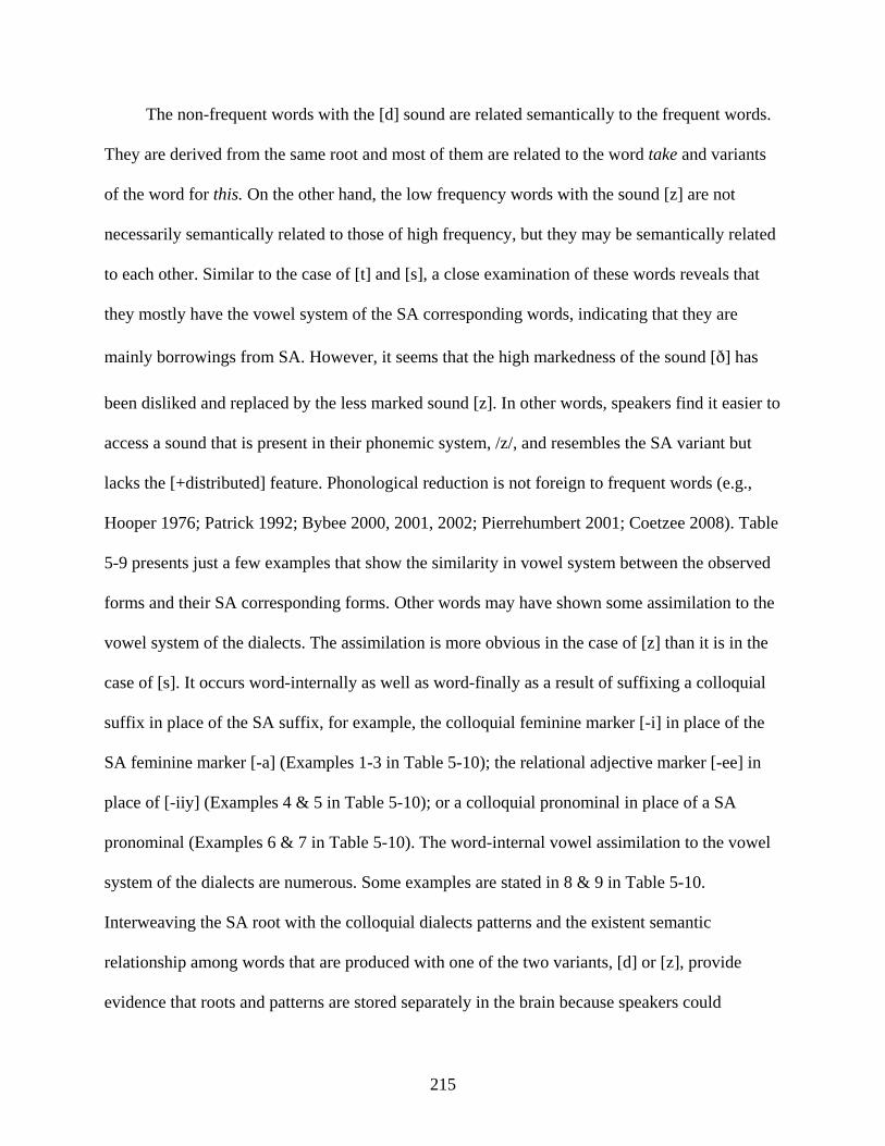
215
The non-frequent words with the [d] sound are related semantically to the frequent words.
They are derived from the same root and most of them are related to the word take and variants
of the word for this. On the other hand, the low frequency words with the sound [z] are not
necessarily semantically related to those of high frequency, but they may be semantically related
to each other. Similar to the case of [t] and [s], a close examination of these words reveals that
they mostly have the vowel system of the SA corresponding words, indicating that they are
mainly borrowings from SA. However, it seems that the high markedness of the sound [] has
been disliked and replaced by the less marked sound [z]. In other words, speakers find it easier to
access a sound that is present in their phonemic system, /z/, and resembles the SA variant but
lacks the [+distributed] feature. Phonological reduction is not foreign to frequent words (e.g.,
Hooper 1976; Patrick 1992; Bybee 2000, 2001, 2002; Pierrehumbert 2001; Coetzee 2008). Table
5-9 presents just a few examples that show the similarity in vowel system between the observed
forms and their SA corresponding forms. Other words may have shown some assimilation to the
vowel system of the dialects. The assimilation is more obvious in the case of [z] than it is in the
case of [s]. It occurs word-internally as well as word-finally as a result of suffixing a colloquial
suffix in place of the SA suffix, for example, the colloquial feminine marker [-i] in place of the
SA feminine marker [-a] (Examples 1-3 in Table 5-10); the relational adjective marker [-ee] in
place of [-iiy] (Examples 4 & 5 in Table 5-10); or a colloquial pronominal in place of a SA
pronominal (Examples 6 & 7 in Table 5-10). The word-internal vowel assimilation to the vowel
system of the dialects are numerous. Some examples are stated in 8 & 9 in Table 5-10.
Interweaving the SA root with the colloquial dialects patterns and the existent semantic
relationship among words that are produced with one of the two variants, [d] or [z], provide
evidence that roots and patterns are stored separately in the brain because speakers could
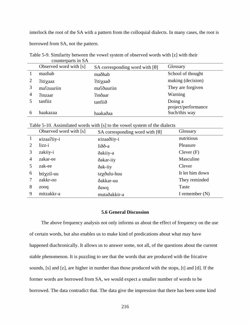
216
interlock the root of the SA with a pattern from the colloquial dialects. In many cases, the root is
borrowed from SA, not the pattern.
Table 5-9. Similarity between the vowel system of observed words with [z] with their counterparts in SA
Observed word with [s] SA corresponding word with [] Glossary 1 mazhab mahab School of thought 2 itiaaz itiaa making (decision) 3 mazuuriin mauuriin They are forgiven 4 inzaar inaar Warning 5 tanfiiz tanfii Doing a
project/performance 6 haakazaa haakaaa Such/this way Table 5-10. Assimilated words with [s] to the vowel system of the dialects Observed word with [s] SA corresponding word with [] Glossary 1 izaaiiy-i izaaiiy-i nutritious 2 lizz-i li-a Pleasure 3 zakiiy-i akiiy-a Clever (F) 4 zakar-ee akar-iiy Masculine 5 zak-ee ak-iiy Clever 6 btizil-uu taulu-huu It let him down 7 zakkr-oo akkar-uu They reminded 8 zooq awq Taste 9 mitzakkr-a mutaakkir-a I remember (N)
5.6 General Discussion
The above frequency analysis not only informs us about the effect of frequency on the use
of certain words, but also enables us to make kind of predications about what may have
happened diachronically. It allows us to answer some, not all, of the questions about the current
stable phenomenon. It is puzzling to see that the words that are produced with the fricative
sounds, [s] and [z], are higher in number than those produced with the stops, [t] and [d]. If the
former words are borrowed from SA, we would expect a smaller number of words to be
borrowed. The data contradict that. The data give the impression that there has been some kind
217
of influx of SA borrowings into the dialects, but this influx stopped at a certain point in time for
some reason. The data give a sense of creeping foreign elements that were stopped by an
opposing force. This leads to the question: what is this opposing force?
We have observed one list of words for each of the sounds, [t] and [s] and [d] and [z]. The
most frequent words maintain the stops; the least frequent ones maintain the fricatives, although
few words produced with the fricatives show very high frequency. If we only take markedness or
“the emergence of the unmarked” (McCarthy and Prince 1994) into consideration, we would
expect to have more words pronounced with [t] and [d] than with [s] and [z] because fricatives
are more marked than stops (*[+cont] >> *[-cont]) cross-linguistically (Clement 1990; Roca and
Johnson 1999; Lombardi 2003). In addition, [t] is the least marked consonant because it is
“unmarked for all features” (Frisch, Broe, and Pierrehumbert 1998:23). In other words, it is
underspecified for dorsal, labial, [-anterior], [+distributed], lateral, round, [+continuant], and
[+continuant, -strident]. All of these features add some kind of markedness to a sound. [t] is
simply characterized as a [coronal] and [-voice], which are the least marked among all the
mentioned features. For example, in English, words such as [in] ‘thin’ and [is] ‘this’ are
replaced by some speakers with [tin] and [dis] respectively (Labov 1972a), not [*sin] and [*sis].
One would expect more words produced with [t] and [d] not only based on markedness but also
due to the complete merger that happened in the 14th century between the SA interdentals [] and
[] and the stops [t] and [d] respectively (Daher, 1998a, 1999; Schmidt 1974). The situation is
the contrary; we find more words produced with the fricatives [s] and [z] as a result of the second
historical change that occurred sometime after the 14th century (Birkeland 1952; Schmidt
1986:57; Schulz 1981:33; all cited in Daher 1999). However, this change did not seem to affect
certain words that are produced with [t] and [d] (i.e., the most frequent words of all). It stopped
218
at a certain point, affecting mainly the least frequent words, which are supposedly borrowed
from SA and replaced by the colloquial Arabic phonology, in our case /s/ and /z/.
To explain the current split between lexical items that are totally produced with the stops
and others that are completely produced with the fricative, we may have to follow one of two
possibilities. The first possibility will be to refute the theory of a complete merger in the 14th
century between stops and interdentals (Daher, 1998a, 1999; Schmidt 1974), that is traces of
interdentals continue to surface, although not as interdentals, rather as fricatives. Refuting the
first theory leads to refuting the second theory of a second change after the 14th century, which
introduced the fricatives in place of the interdentals (Birkeland 1952; Schmidt 1986:57; Schulz
1981:33; all cited in Daher 1999). Refuting this theory will be accompanied with then suggesting
that the historical change only affected highly frequent words on the basis of usage-based models
(Bybee 2001) or exemplar-based models (Pierrehumbert 2001). These models propose that
words of higher frequency are more prone to reduction. Non-frequent words are less affected by
change and usually retain their original form or features. Thus, one can assume on these grounds
that highly frequent words, such as haadaa and ktiir, historically underwent reduction of the SA
features [+continuant] and [+distributed], but the least frequent words did not. However, there
are no traces of interdentals in natural speech. In addition, refuting this theory does not explain
the two lists of words with fricatives, such as masalan and izaa, instead of the SA interdentals.
These two lists also show reduction of the feature [+distributed]. The few high frequency words
with the fricatives do not behave like other highly frequent words that have also reduced the
[+continuant] feature. They seem to have resisted this type of reduction. Why would some
frequent words resist one reduction and not the other? In other words, why would some frequent
words show reduction of two features and others show reduction of only one feature?
219
Furthermore, if there was not a complete merger, we would expect some kind of variation and
probably a balanced number of words with the stops and the fricatives. We actually have no
variation and continue to have a large number of words produced with fricatives and less words
produced with stops. It seems this possibility cannot completely explain the present split among
stops and fricatives. Consequently, we have to take the second theory into consideration. That is,
a second change happened some time after the 14th century and led to this stable phenomenon.
Taking the second theory into account implies accepting the first theory too. Furthermore, a
support of the merger theory comes from Churchyard’s (1993:335) historical study. He
mentions, in a footnote, “[t]hat *θ, *θ, and * actually remained distinct in Old Aramaic is seen
from the fact that in later Aramaic these sounds merged with the dental/alveolar stops *t, *t, and
*d, respectively”16. These historical sound variation and changes, according to Churchyard, may
have developed in some dialects before others and then they gained prestige to the point that they
started to gain importance and prestige in other dialects later on, leading to the spread of the
change to other dialects and eventually a merger. Since Arabic is Proto-Semitic language and
most of its sound system (twenty-one out of the twenty-eight letters in Arabic were borrowed
from the twenty-two Aramaic Alphabet) was adopted from Aramaic, a similar change and a
merger may have happened in Arabic. This seems to be a feature of Proto-Semitic languages in
which similar shifts and mergers have occurred historically and have influenced each other, as is
16 The asterisk before each of the sounds in the quotation is used to indicate a variable, not a variant. The symbol *θ is used to refer to a dental/alveolar emphatic fricative; *t is the symbol used to refer to dental/alveolar emphatic stop. These two symbols are represented in IPA as and t respectively.
220
the case of the influence of Aramaic dental/alveolar *s sound shift ([] → [s]) on the Hebrew *s
sound shift ( [] → [] and []→ [s])17.
This brings us to the second possibility and back to the role of frequency in this stable
phenomenon. According to Bybee (2001:11), “token frequency”18 has two main effects. In one
effect of frequency “phonetic change often progresses more quickly in items with high token
frequency”. Pierrehumbert (2001:3) argues on the basis of Bybee’s (2000, 2001) theory of usage-
based phonology that “leniting historical changes are more advanced in frequent words than in
rarer ones.” Thus, high frequency words are more likely to undergo change, mainly reduction.
For example, the deletion of [t] and [d] word-finally post-consonantally is more common in
English in highly frequent words, such as went, just, and and, than in infrequent words (Guy
1991; Santa Ana 1992; Bybee 2000; Phillips 2006; Coetzee 2008; Coetzee and Pater 2008). This
is an example of a whole segment reduction, but reduction could include feature reduction for the
purpose of minimizing articulatory effort (Saussure 1959, Martinet 1964) (i.e., easier and simpler
articulation). This first frequency effect proposed by Bybee (2001) can explain the first historical
change towards the use of [t] and [d] in place of [] and [] respectively. The SA interdentals
were reduced to full stops; the features [+distributed] and [+cont] were eradicated. This merger
apparently happened gradually, affecting the most frequent words first and then the least frequent
ones.
The second effect of token frequency contradicts the first effect, because “it makes items
more resistant to change” (Bybee 2001:12). In other words, high frequency words become
17 *s refers to voiceless lateral fricative. [] stands for (alveo)palatal fricative-lateral that existed in early first millennium B.C.E. Hebrew. [] stands for dental/alveolar fricative-lateral that existed in early first millennium B.C.E. Aramaic.
18 “Token Frequency” to the frequency of the occurrence of a word.
221
resistant to a new swiping change because they have already developed an automatized
production (p. 12). Because “tokens of use map onto existing representations, high-frequency
items grow strong and therefore are easier to access” (p. 28). Bybee (2001:12) refers to this type
of resistance as “conserving” effect, rendering some words more “conservative” in the face of
change. For her, the frequency of words
gives them a high level of lexical strength. That is, they are so engrained as individual patterns that they are less likely to change even if general changes are occurring in the language. To account for this entrenchment effect, I have proposed (Bybee 1985) that representations are strengthened whenever they are accessed. This strengthening makes them subsequently easier to access and also more resistant to some forms of change.
This second effect of frequency, as proposed by Bybee (2001), can account for the
existence of [s]- and [z]-words alongside the [t]- and [d]-words that resulted from the 14th
century merger. It seems that the second historical change that occurred sometime after the 14th
century (Birkeland 1952; Schmidt 1986:57; Schulz 1981:33; all cited in Daher 1999) did not
affect the most frequent words in the dialects (i.e., words that are produced with the stops, [t] and
[d]). We have observed in the data that the most frequent words are those produced with the
stops with few exceptions that are produced with the fricatives, [s] and [z]. The findings of this
study support Bybee’s (2001) usage-based theory, which provides explanation to the current
stable situation of the use of [t] and [s] and [d] and [z]. For Bybee (2003), “repetition” and “high
frequency” develop ‘automatization” and “autonomy” that lead to “entrenchment”. In this sense,
the highly frequent words produced with the stops were not affected by the second historical
change because they became entrenched in their own phonemic representation. I avoid here
using Bybee’s (2001) suggestion that words are stored as whole units in the lexicon because of
their autonomy. In a language like Arabic that has a more complex morphological system, this
may not be case. Bybee’s suggestion was actually critiqued by Pierrehumbert (2002) in her
review of Bybee’s (2001) book. Pierrehumbert suggests that
222
the case for excluding morphemes in addition to words is less firm. Even in English, and even for infants, words are normally extracted from running speech rather than learned in isolation; positing a mental lexicon of any and all effectively extractable chunks might provide a better basis for the analysis of more complex morphological systems. (2002:462)
The case of how words and morphemes are stored in Arabic requires further
investigation. Suggesting that words become entrenched in their phonemic representation does
not violate the view that words could be “storage units” (Bybee 2001; Beret, Vaknin, and Marcus
2006) or morphemes could be stored separately (Feldman, Frost, and Pnini 1995; Pierrehumbert
2002).
5.7 Conclusion
In conclusion, Bybee’s (2001) usage-based theory with its two frequency effects provides
an explanation to the current stable phenomenon regarding the use of the four variants [t] and [s]
and [d] and [z] in the naturally occurring speech of rural migrant speakers to the city of Hims.
The two frequency effects of the usage-based theory support the theories of two different
historical changes. It is because of those two historical changes and frequency effects that we
have two different categories of words for each of the SA interdentals. The first change led to the
loss of the two features [+distributed] and [+continuant] from the SA interdentals. The second
change began with borrowing a large number of words from SA. Instead of using the marked
sounds [] and [], speakers apparently sought in their native phonology similar sounds that are
less marked, [s] and [z]. This is not surprising for a people that grew accustomed to producing
much less marked sound, [t] and [d]. Borrowing the SA forms was, thus, accompanied in this
case with one feature reduction instead of two, [+distributed]. This case of seeking native
phonology is observed in an example given by Morris (2000:14) in an endnote. The example
presents the case of the Peninsular dialect of Chinato, native to the province of Cáceres
(Extremadura), in which there is no underlying /s/. Instead, the dialect has only // (spelled with
223
‘s’, ‘c’, or ‘z’), which is realized as [h] in syllable coda (2000:14). Because [] is highly marked
in that dialect, it is replaced with the native dialect phonology (i.e., /h/). Although I have been
able, to a great extent, to explain the reason behind this stable phenomenon, I still think that
further research is required in this area to confirm these findings.
Although the speech sample is taken from only RCA speakers, it is my belief that the same
pattern applies to HCA speakers. It is also believed to be a characteristic of big urban centers in
Arab countries, such as Amman (Abdel-Jawad 1986). This pattern may differ in Bedouin dialects
or in other Arab dialects. In Bahrain, for example, Holes (1986) actually notes a kind of
convergence towards the SA variant [] away from the non-standard form [f]. For him, this
variation is led by social factors such as religious denominations and social identity as well as the
influence of SA through education. The [] is used by the ‘Arab, the “Sunni descendents of the
Bedouin tribes” (p. 33) whose dialect is perceived as prestigious. This example among others
calls for investigating similar phonological changes, in which the marked interdentals are used. It
seems their use and variation may depend on different factors in different settings and require
explanation from different angles.
224
CHAPTER 6 CONCLUSION
6.1 Introduction
In the first chapter, a number of research questions were set forth for investigation. This
chapter aims not only to give a brief summary of the answers to each of those five research
questions but also to summarize other findings that emerged throughout the study. I will first
provide an answer to each question individually, based on the findings in the various analysis
chapters. I will then provide some advantages of and caveats concerning the new model
proposed in this study. Then, I will touch on the role of frequency effects in this study. I will also
present some implications, directions and recommendations for future research. I will conclude
this chapter by emphasizing the importance of combining both the social and linguistic in one
linguistic theory.
6.2 Use of OT and the GLA to Account for Switching between Two Different Dialects and Inter- and Intra-speaker Variation
Research question 1: How can Optimality Theory account for speakers’ switch between
two different dialects and their intrapersonal and interpersonal variation in the use of particular
sounds (e.g., the use of [] in place of [q]) based on their interlocutor’s background?
To answer this question, I developed a new model for analyzing sociolinguistic variation,
employing OT and the GLA. In this model, I proposed a number of social constraints in addition
to more conventional linguistic constraints of OT and the GLA, although the particular linguistic
constraints themselves may not have been proposed previously. I treated social constraints in the
same way that linguistic constraints are treated in the GLA. They are given a continuous scale of
ranking values and are subject to the continuous ranking of stochastic grammar. In other words,
their ranking values may differ from one speaker to another and from one group of speakers to
225
another. I have shown that the interaction of those social constraints with linguistic constraints
yields results that match real life occurrences. I have also shown that the choice of the right type
and number of social constraints determines the grammar of an individual or a group of
individuals at a certain time and place. In order for a speaker to acquire the new form, [],
completely, s/he has to change the ranking values of two constraints of his/her mother dialect,
RCA. Speakers who can switch between the two forms [q] and [] with one hundred percent
accuracy have acquired the new ranking values with one hundred percent accuracy, in that they
do not have overlapping among certain constraints. Thus, they sound city-like because of
acquiring the new grammar, and thus, the new form completely. In those speakers, certain social
constraints rank very high, affecting their choice of a ranking value at a certain time and place.
Speakers who show intra- and inter-speaker variation in the use of [q] and [] with the
same interlocutor have not acquired the new ranking values of the constraints completely. The
ranking values of constraints become very close to each other, and to the constraints of their
mother dialect, leading to overlapping of constraints. This overlapping leads to variable outputs.
The degree of variation relies on the type and number of social constraints involved. For
example, a speaker or a group of speakers that uses [q] 85% and [] 15% may have more social
constraints or different social constraints involved than a speaker or a group of speakers that uses
[q] 65% and [] 35%. I would like to add that some social constraints might rank higher than
other social constraints in some speakers, leading also to inter-speaker variation.
OT and the GLA not only account for sociolinguistics variations, such as the variable use
of [q] and [], but also for other types of phenomena that may occur within the same speech.
They have the advantage of accounting for two different variations independently from each
226
other. For example, the use of the sounds [t] and [s] and [d] and [z] is a stable situation in the
naturally occurring speech of rural migrant speakers to Hims. OT and the GLA have been able to
deal with this phenomenon separately from the sociolinguistic variation between [q] and []. One
variation does not necessarily affect the other. In the case of the variants [t] and [s] and [d] and
[z], OT and the GLA have shown that faithfulness to the input is the major factor that determines
the output, in contrast to the variable use of [q] and [], in which faithfulness constraints are
easily violated.
6.3 Incorporating Social Factors into the GLA
Research question 2: How can social factors be incorporated into the GLA?
I implemented social constraints as part of OT and the GLA like linguistic constraints.
They interact with linguistic constraints to represent what goes on in the brain of speakers during
speech production because of their social surroundings. I showed that their interaction with
linguistic constraints is essential to give percentages that match real life occurrences. I treated
these social constraints like stochastic constraints on a continuous scale. The ranking value of
these social constraints may differ from one speaker or group of speakers to another. The
difference in their ranking values among speakers reflects the difference in real life percentages.
For example, the social constraint *M[] may be higher ranked than *F[] because women are
more socially conscious of the prestige associated with the form [] than males are, particularly
older females. The higher ranking value of *M[] leads to higher percentages of use of [q] by
males than by females. In addition, some social constraints form groups together and work as
one family. For example, older female speakers from Akrama should have all of the following
social constraints higher ranked than other constraints to maintain their mother dialect form [q]:
227
*F[], *OLD[], *AKR[]. Conflict may arise when speakers employ constraints that militate
against two opposing sounds (i.e., more variation results from such implementation).
Furthermore, incorporating social constraints in the computation explains the variable use of [q]
and [] among members of the same social groups or different groups. In addition, certain social
constraints give expectations on what the speech of a certain speaker or group of speakers should
sound like.
6.4 Role Played by Social Factors
Research question 3: To what degree do social factors play a role in building our
grammars, or rather developing new grammars?
We have noticed that the intersection of social constraints with linguistic constraints
provides a clear picture of what goes on in the mind of a learner of a new dialect (usually
prestigious urban dialects). The social constraints that are involved determine the percentages of
the occurrence of each variant in the naturally occurring speech of rural migrant speakers. The
degree of the social awareness, which is related in this study to the ranking value of the social
constraints, affects the choice of a certain variant over another. Thus, if the social constraints that
impose the use of the urban prestigious variant have high-ranking values (i.e., are highly valued
by speakers), such as *F[q] and *OLD[q], the prestigious form is more likely to be produced. If
they are ranked low, the mother dialect form is more likely to be produced. The latter situation
reflects the importance of the mother dialect social values in the speech of those speakers. In
speakers who do not show acquisition of the new form, the ranking values of their mother dialect
social constraints are fixed and do not change, particularly in the speech of older speakers. In
such situation, social constraints such as *F[] and *OLD[] would be highly ranked, whereas
social constraints such as *F[q] and *OLD[q] would be low ranked. I have compared this to
228
species that, when fully developed in their environment, are less likely to change and develop
later on in life. They maintain their features and move on with life. One should, in any case,
consider that whether speakers adopt the new ranking values of social constraints or not, these
social constraints affect the way they speak and the type of grammar chosen at a particular time
and place. If they are affected by their new environment and the new social constraints, they tend
to vary their speech and some of them my reach complete levels of acquisition of the new form.
If they are not influenced by the urban society’s values, they retain their rural community social
values and continue to produce their native form almost invariably.
6.5 Consistency of Variation
Research question 4: How consistent is the pattern of variation and sound change within
and among rural migrant speakers to the city of Hims?
Concerning the two variants [q] and [], intra- and inter-speaker variation has been
observed. Thus, some speakers showed not only variation in their speech within the same
conversation but also correction towards the new form. In addition, varying speakers differed
from each other in the degree of usage of each variant. Other speakers used either the [q] sound
or the [] sound invariably. Thus, the variable use of [q] and [] is not consistent. There is a clear
inter- and intra-speaker variation. We have seen that social factors play a major role in this
variation, particularly age. Younger speakers are more inclined towards the urban form, [],
whereas the majority of older speakers are more inclined towards the [q] sound. Females are
more inclined towards the prestigious form [] than men are. Actually, men, mainly elderly men,
are more inclined towards the [q] sound. Furthermore, residents of Al-Hameeddieh show higher
usage of [] than residents in Akrama because of their environment, which is more linguistically

229
demanding in Al-Hameeddieh than it is in Akrama. This inconsistency is reflected in both the
statistical analyses and the ranking values of social and linguistic constraints.
As for the variants [t] and [s] and [d] and [z], speakers have shown consistency in their use.
All speakers – young and old, males and females, upper- and middle-class, and residents of both
residential areas, Akrama and Al-Hameeddieh – use a certain variant with certain words and the
other variant in other specific words. I have called this a stable variation because of the observed
consistency among speakers. This phenomenon developed historically because of two different
changes: one that led to a merger between the SA forms [θ] and [ð] and the stops [t] and [d]
respectively; the second led to the introduction of [s] and [z] in place of the SA forms [θ] and [ð]
as a result of lexical borrowings from SA.
6.6 Markedness Constraints versus Social Constraints
Research question 5: Which factors are stronger in leading a sound change: markedness
constraints or social constraints?
We have seen that in the variable use of [q] and [], social constraints play a major role in
determining the grammar chosen at a particular time and place. In this type of variation, social
constraints are the ones leading the present change towards the prestigious form more than
linguistic markedness constraints do, although one cannot completely eliminate the effect of
markedness on this type of variation. First, the glottal stop is less marked cross-linguistically
than the uvular voiceless stop. It lacks the [RTR] feature that is characteristic of the [q] sound.
According to radical underspecification, the positive value of a feature is the marked one and the
negative value is the default, unmarked one (Archangeli 1984, 1988). In an endoscopic study of
tokens of / h/ spoken by a Jordanian Arabic speaker, Zawaydeh (1999) found that no retraction
of the tongue root accompanied these two segments. Thus, they are considered underspecified

230
for place, which makes them less marked than other consonants. This finding is supported by a
number of phonological analyses of laryngeals (e.g., Clements 1985; Steriade 1987; Kenstowicz
1994; Rose 1996), which have indicated that / h/ are produced with only a glottal gesture,
rendering them placeless. This makes Glottal the least marked place of articulation in many
languages, allowing for the following hierarchy *[LAB] >> *[DOR] >> *[COR] >> *[Glottal].
The unmarkedness of the glottal stop //, for example, can be observed in its use as an
epenthetic consonant in Arabic (Holes 2004) and many other languages to avoid onsetless
syllables, such as Malay (from the Austronesian language Bahasa Melayu/Indonesia as spoken in
Malaysia) (e.g., El-Imam and Don 2005). Shahin (2002:60) argues that all word-initial glottal
stops in Arabic are epenthetic and the evidence “is that they are not observed when another
consonant can serve as onset of the word-initial syllable.” For example, in Palestinian Arabic,
[ik.tib] ‘write’ is possible, but not *[ik.tib] or *[bi.-ik.tib]19.
The unmarkedness of [] may have led historically to the merger of [q] with [] (Abdel-
Jawad 1981; Haeri 1996: 122) in major urban areas, such as Hims (Habib 2005), Damascus
(Daher 1998a), Cairo (Haeri 1991), Amman (Abdel-Jawad 1981), etc. This merger, according to
Garbell 1978 [1958]) occurred sometime between the 11th and the 15th centuries. However, the
role of markedness in the variable use of [q] and [] is not limited to the historical linguistic
markedness of [q] in comparison to the unmarkedness of []. If we look closely at the social
constraints that have been employed in this study, we find that they are mainly markedness
constraints that militate against the use of a certain variant by a speaker or a group of speakers.
19 Dots indicate syllable boundary; hyphens indicate morpheme boundary; and asterisks indicate ill-formedness/ungrammaticality.
231
Thus, those social constraints that are pertinent to what is prohibited, allowed or expected in
certain communities are one type of markedness constraints. In the current synchronic variation,
they play a more pronounced role than linguistic markedness constraints in determining the
grammars of the various speakers. Those affected by the urban markedness constraints tend to
vary their speech. On the other hand, those who maintain their mother dialect forms show their
maintenance or clinging to the social values of their native communities, and thus are affected by
the markedness social constraints that are pertinent to their communities. This could also be
viewed as the effect of faithfulness to their social values.
As for the four variants [t] and [s] and [d] and [z], social constraints did not seem to play
any role in this phenomenon. The study has indicated that markedness may have played a role
historically in pronouncing the SA variants [θ] and [ð] as [t] and [d] respectively. The merger
with these two sounds was completed around the 14th century (Daher, 1998a, 1999; Schmidt
1974). In addition, the use of [s] and [z] in place of [θ] and [ð] of the borrowed words from SA is
another indication of the role of markedness in the second diachronic change which took place
some time after the 14th century (Birkeland 1952; Schmidt 1986:57; Schulz 1981:33; all cited in
Daher 1999). There is ample evidence from Arabic and other languages that show that the
sounds [θ] and [ð] are marked. Morris (2000:3), for example, indicates that the realization of
Spanish aspirated /s/ and // as [h] word-finally and sometimes word-internally are cases of the
emergence of the unmarked, e.g., diez /die/ may surface as die[h]. Today, markedness is no
longer playing a role in the use of the four variants [t] and [s] and [d] and [z]. What maintains the
pronuncation of each of the four variants as it is are faithfulness constraints. Each of the four
variants has its identical underlying form, which represents the input in OT. This input is
protected by faithfulness constraints to appear as it is in the output.
232
6.7 Advantages of and Caveats about the New Model
6.7.1 Advantages of the New Model
The five questions that started this work led to the development of a new model that has
the following advantages:
1. It gives mental representation of the interaction between social and linguistic
constraints and the effect of each type of constraints simultaneously. The results have
shown how the GLA can model sociolinguistic variation by incorporating the right
type and number of social constraints. The continuous approach to constraints allows
for great degrees of optionality and variation. The results show that social constraints
should constitute an important part of linguistic theory, as they play a major role in
determining our grammar at a certain time and place. It is social constraints that
influence our degree of acquisition of the ranking value of constraints and the degree of
usage of each of the sociolinguistic variants, [q] and []. Giving mental representations
of the various individual and group grammars in a sociolinguistic variation situation
endows the model and the proposed constraints with a psychological reality (Section
1.1). The second, third, and fourth advantages of the model also draw our attention to
the psychological reality of the proposed constraints and the accompanying
sociolinguistic process.
2. This new model not only presents what goes on in the human’s brain when a
sociolinguistic variation is in process but also gives predications on what variation
would look like if certain constraints are involved. A listener can predict from listening
to the speech of an interlocutor what type of grammar or constraints are involved. If
that listener is a rural migrant and the interlocutor is another rural migrant who displays
233
some kind of variation between the rural and the urban forms, s/he will most likely
notice the interlocutor’s variable use and the social constraints involved in this
variation. For instance, a male listener to an older female speaker from Al-Hameeddieh
knows that she activates the two constraints *F[q] and *OLD[]. These two constraints
have also opposing effects: one of them militates against the use of [q] and the other
one militates against the use of []. This could be a further reason for the occurrence of
variation in a certain speaker or group of speakers. Opposing social constraints may
create conflict between the social meaning associated with each variant in a speaker’s
brain, leading to overlapping of constraints and consequently variation.
3. The model further reflects on each individual’s or group of individuals’ linguistic
environment because the degree of input of a form affects the degree of acquisition of
that form. A speaker who has ample contact with urban interlocutors is more likely to
have higher degree of acquisition of the new form than a speaker who is surrounded
with rural speakers most of the time, as was the case when comparing Al-Hameeddieh
speakers to Akrama speakers.
4. It has also been observed during applying this new model that because of the young
speakers’ early contact with the urban form, they tend to acquire it and use it all the
time. The model, in this case, predicts that the younger speakers have reconstructed
their input despite their initial exposure to their parents’ rural form, [q]. In other words,
their input becomes the urban form, //. They restructured their input not only because
they are in contact with a new form but also because they notice the prestigious social
value of the urban form. As many may know, children are very sensitive to comments
and criticism. They do not like to be stigmatized or ridiculed by their peers or friends
234
because they do not sound like them. As soon as these children notice the new form
and the stigma associated with their parents’ form, they decide to adopt the new form.
In their early stage of acquisition, it is easy to restructure their input and sound more
urbane than their parents are. We have seen exceptions among three young male
speakers who have lived all their lives in Akrama. Because of their less demanding
environment to learn the new form, they retain their parents’ form. However, all the
other young speakers, who are likewise the sons and daughters of rural migrants, show
complete acquisition of the new form in just the span of one generation, as is the case
of the sons and daughters of rural migrant speakers to Cairo (Miller 2005).
5. The model not only accounts for sociolinguistic variation but also other accompanying
phenomena that may be led by different factors. This is an important aspect of the
GLA, its ability to account for categorical and optional ranking values. The GLA has
enabled me to account for the use of the variants [t] and [s] and [d] and [z] separately
from the sociolinguistic variation between [q] and []. It has shown that social
constraints do not play a role in the case of the former four variants, although they play
a role in the variable use of [q] and []. It has further shown that the consistent
occurrence of each variant in certain words is the result of the categorical higher
ranking of faithfulness constraints with respect to other constraints.
6. Where statistical analyses fail to indicate a specific influence of a social factor on the
variation observed, the new model provides evidence of the effect of that factor
because of the model’s more refined specificity. Each social factor is divided into a
balanced number of constraints in relation to its categories and the sociolinguistic
variants. A social factor such as residential area could be divided into four social

235
constraints if there are two residential areas and two variants. Thus, the constraints are
calculated in a factorial manner, multiplying the number of the social factor categories
with the number of the sociolinguistic variants. This specificity allows, for example,
for only one of the four constraints to be involved in the computation. In Section 4.4.4,
I have shown that the statistical analysis fails to show significant interaction between
residential area and gender and age, regarding the variable use of []. However, the
results of Example 7 in Chapter 3 have shown that young female speakers from Al-
Hameeddieh must rank all three constraints – *F[q], *YOUNG[q], and *HAM[q] –
higher than * to achieve 98% pronunciation of [] and 2% of [q]. Thus, the social
constraint, *HAM[q], which constitutes one of the four social constraints of residential
area, is implemented in the speech of young female speakers from Al-Hameeddieh to
produce high percentages of [].
6.7.2 Caveats about the New Model and Other Limitations of the Study
A researcher should know the speech community well to be able to discover the social
constraints that are involved in the variation and the learning process. It was feasible for me to
investigate the speech of rural migrant speakers to the city of Hims because I am a close member
of that community. I know the participants well. I know their life styles and the community’s
social evaluation for each one of them. I also know the culture and the social values and behavior
associated with each linguistic form. This is not only knowledge on my part but also on the part
of many speakers who have expressed throughout their conversations the stigma associated with
[q] and the rural dialects. They also mentioned who they think tend to change their speech the
most (i.e., older females). In addition, some of them pointed out some of the reasons that rural
speakers tend to change their speech (Habib 2005, Sections 5.2 and 5.3).
236
The model cannot converge on a simple categorical grammar for multiple varying
speakers, which is normal because the ranking values of constraints are very close to each other,
leading to overlapping of constraints, and hence variation. Because the model cannot converge
on a strictly dominated grammar, one can only predict continuous variation and the present
percentage usage of each variant in speakers. One cannot predict if a varying speaker can acquire
the new form completely. The only way to make such prediction is to manipulate the pair
distribution in the GLA and make speakers learn from partial outputs that are considered
potential input. Changing the amount of input that a speaker receives of each variant can change
the result in the direction of convergence towards one grammar or the other. However, in the real
world the exact percentages of input are hard to determine; there are many factors that can play a
role in determining the input intake, which is very hard to determine without observing a speaker
over a very long period of time or for the rest of his/her life. Although it is beyond the scope of
this study, it is worth mentioning that I have noticed during the examination of the speech of one
older female speaker whom I recorded in 2004 and 2006 that she has progressed more, in two
years, towards the prestigious form. More observations of this type throughout upcoming years
are essential to understand and arrive at conclusions on how language change progresses in a
society.
Although this study did not cover all the possible social factors that could be involved in
the variation under investigation, it introduced a new model of sociolinguistic analysis that could
be improved and expanded on. It may be a good idea to include social factors, such as religion,
social status, and social distance in future studies. It may also be a good idea to have more than
one interviewer conduct the interviews with the same interviewees (Walters 1991). The
background of the interviewer may have influenced the way speakers speak. I would expect
237
speakers to use the [] sound more frequently with a speaker who is originally from the city of
Hims, for example. Because interviewees in this study are very close relatives and friends to me,
they may have felt more comfortable using their native form, [q], with me, particularly in the
case of Speakers 29, 30, and 31. According to their sister (i.e., Speaker-44), those three young
male speakers who reside in Akrama change their speech towards the prestigious form, [], when
conversing with urban interlocutors or strangers, particularly from the opposite sex. This was not
the case when I interviewed them. My explanation of this situation is that they felt very
comfortable talking to me in their native form, [q], because of their strong familiarity with me.
They know that I am familiar with their rural form and the way people from Oyoun speak. They
also know that I will not be critical of that rural form because my parents use it with us all the
time.
6.8 Frequency effects
Although frequency was not a part of the research questions that led this work, I felt that it
was essential to examine the influence of frequency of words on the acquisition process of the
urban form []. The examination of word frequency was even more important in the case of the
four variants [t] and [s] and [d] and [z], because this stable phenomenon cannot be explained by
social factors, as all speakers are consistent in using them. The results show that frequency has
varying roles with respect to the two types of variations that are dealt with in this work.
Frequency has a facilitative learning effect concerning the sociolinguistic variation between [q]
and []. In other words, it is not the factor that leads the change from [q] to []; rather, it is the
leading factor for acquiring highly frequent words faster than less frequent words which contain
238
the prestigious form []. Thus, frequency, in this case, plays a major role in determining which
words a varying speaker acquires initially.
As for the use of the variants [t] and [s] and [d] and [z], frequency has two opposing
effects. The first effect led to the historical merger between the SA [θ] and [ð] and the stops [t]
and [d] respectively. The second effect safeguarded the most frequent words that contain the [t]
and [d] from another historical sweeping change (i.e., from the use of [s] and [z] in place of the
SA [θ] and [ð] in borrowed words). Very frequent words develop with time some kind of
autonomy or automatization because of continuous repetition (Bybee 2001); they develop a
strong mental representation that makes them easier to access and more resistant to change.
6.9 Implications, Directions and Recommendations for Future Research
For a long time phonological theory and sociolinguistic theory acted independently from
each other. In this work, I was able to bring these two subfields together. Linguistic theory
should be general enough to account for not only the phonological aspect of grammar but also
the social aspect of that grammar. Researchers who are interested in factors other than social
factors may find the new model helpful in accounting for psychological, pragmatic, or other
factors within the same framework. I would not want to make the claim that the model is perfect
in its present shape. I believe more work and modifications may need to be done to improve the
model. It needs to be tested on other languages and other social constraints. The development of
the model does not stop at the application of the social constraints proposed in this study. Rather,
it should extend to the proposition of other social constraints that may be pertinent to different
sound changes in different speech communities.
One important implication of this study is the possibility of generalizing the proposed
social constraints to other languages. Many sociolinguistic studies have shown similar results
239
regarding the increased use of prestigious forms by women, younger generations, or residents of
prestigious areas (e.g., Labov 1972a; Gal 1979; Milroy 1980; Eckert 1991b; Miller 2005). These
similar results prompt me to propose some general social constraints that can be applied to any
language and any linguistic form. At the same time, there are studies that have shown
contradictory results. Thus, the ranking values of those social constraints are the determining
factor of what form is chosen at a certain time and place by a certain speaker or group of
speakers. Those ranking values, in this sense, may differ from one speech community to another
or from one language to another. Because not all speech communities evaluate sounds in the
same way, one should always take into consideration different grammars and different social
constraints. Consequently, generalizing the social constraints does not have negative effects
because those general constraints could be higher or lower ranked in one speech community or
another. The general social constraints that I propose are as follows:
Gender:
*F[SF] Stigmatized forms are marked in the speech of females
*M[SF] Stigmatized forms are marked in the speech of males
*F[PF] Prestigious forms are marked in the speech of females
*M[PF] Prestigious forms are marked in the speech of males
Age:
*OLD[SF] Stigmatized forms are marked in the speech of older speakers
*YOUNG[SF] Stigmatized forms are marked in the speech of younger speakers
*OLD[PF] Prestigious forms are marked in the speech of older speakers
*YOUNG[PF] Prestigious forms are marked in the speech of younger speakers
240
Social class:
*UM[SF] Stigmatized forms are marked in the speech of upper-middle class
*LM[SF] Stigmatized forms are marked in the speech of lower-middle class
*UM[PF] Prestigious forms are marked in the speech of upper-middle class
*LM[PF] Prestigious forms are marked in the speech of lower-middle class
Residential area:
*PR[SF] Stigmatized forms are marked in the speech of prestigious areas
*NR[SF] Stigmatized forms are marked in the speech of non-prestigious areas
*PR[PF] Prestigious forms are marked in the speech of prestigious areas
*NR[PF] Prestigious forms are marked in the speech of non-prestigious areas
Of course, these constraints do not form an exhaustive list of general social constraints;
rather, they are just a subset of the possible general social constraints that can be proposed. One
can even modify these general ones to include more constraints if one is dealing with more than
two variants of the same variable. If there are three variants, then the social factor could be
divided into six constraints. Furthermore, stigmatized forms and prestigious forms in the
constraints’ description could be replaced with the respective sounds under investigation. One
can also take into consideration the length of stay in the city and other factors such as religion,
education, etc.
Proposing general social constraints raises the issue of the universality of the
sociolinguistic behavior of speakers across languages. This is a wide topic to explore in future
research. Questions such as the following may occur. Are human beings endowed with a
universal set of social constraints? Do they eliminate or reactivate some of these constraints
because of their observations of the societal behavior around them? In other words, do they
241
acquire the ranking of these constraints in the same way they acquire the ranking of their L1
linguistic constraints? And do they acquire these social constraints in the same way an L2 learner
acquires the ranking of the linguistic constraints of an L2?
I propose that humans may have universal social constraints in the same way that they
have a universal set of linguistic constraints. Similar to how they acquire their mother tongue by
eliminating or reranking markedness and faithfulness linguistic constraints that are pertinent to
their L1, speakers acquire their social skills from their surroundings and tend to eliminate some
social constraints and rerank social constraints that are pertinent to their environment. Thus, like
linguistic constraints that are universal in nature but their ranking with respect to each other is
language specific, social constraints could be universal in nature and their ranking is language,
dialect, or community specific. In other words, the relativity of the social constraints is
maintained in the specificity of individual grammars and constraint rankings of particular
speakers or communities of speakers. When speakers learn a second language or dialect, they
attempt to change the ranking of those social constraints or reactivate some dormant social
constraints to fit into their new environment. This is true pragmatically. For example, an L2
speaker has to learn the pragmatics of the L2 in order to sound native-like and to integrate into
the new culture. Thus, the idea of universal social constraints is worth exploring in future
research.
One further suggestion for future research is applying the new model to examine the
percentage of usage of [q] and [] in other Arab urban communities (within or outside Syria)
against those found in this study. If percentages match, then there is a similar trend in most Arab
urban communities towards not only the activation of the same social constraints but also the
same ranking values. If percentages do not match, then there might be difference in the ranking
242
values of the same social constraints from one community to another or from one country to
another. In addition, the difference among Arab countries with respect to the use of various
variants as a replacement for [q] calls for further studies to examine those usages against the
usage of other variants in other Arab countries to look for similar or different trends.
The variants [t] and [s] and [d] and [z] are not socially conditioned in the speech of most
Syrian speakers. However, this may not be the case in other Arab countries. Thus, further studies
are needed to investigate if the naturally occurring speech of other Arab dialects has socially
conditioned variations in the use of these four variants. I presented the example of Bahrain
(Holes 1986), in which the SA variant [θ] is considered socially and colloquially prestigious and
there is a kind of convergence towards this form away from the non-standard form [f]. In this
case, social constraints could be included in the GLA to account for the sociolinguistic variable
use of [θ] and [f].
In addition to all the above suggestions, longitudinal observational studies are a good
source of data to make future predictions in the GLA about changes in progress. Such
longitudinal observations could complement this study, in that they could provide the usage
percentages of each variant in varying speakers throughout a number of years. The results may
be informative about the directionality of variation and the change in the input intake of each
variant if there is any. If changes in usage percentages differ throughout a period of time, then
we can conclude that some learnability is taking place despite the speakers’ surrounding varying
linguistic environment. Such results may also be informative about the speakers’ increased or
decreased social contact with speakers of the prestigious form.
Based on my personal observations and the comments of some speakers, I believe it is
important to trace the sound change of [q] into [] in some villages of Wadi Al-Nasara because
243
of contact with urban speakers through marriage or increased commuting between these villages
and urban areas. I believe some villages may show greater use of [] than [q] within the village
itself. Furthermore, some villages may show greater use of [] or [q] than other villages. The
spread of the use of [] to the villages and the difference in spread among these villages is worth
investigating. Such research should focus on children from all ages that live in the villages and
receive their education in the schools of those villages to observe the outside influence on them. I
mean by outside influence any of the following: going to visit relatives in urban areas or []-
speaking areas; mothers from outside the villages that have been married to men in the villages
and brought with them the prestigious form []; and the children’s contact with relatives visiting
from []-speaking area. In such studies, not only children who undergo such outside influences
should be investigated but also other village children who are not directly affected by an outside
influence. They may have minor contact with [] through exposure to television stations that use
the [] sound instead of [q] or through contact with other village children who are exposed to
those outside influences. Starting with observing village children may lead to predicting the
future pronunciation of the villages. In other words, we may be able to foresee a change in
progress in the villages themselves. I believe there is a change in progress in the villages towards
the urban prestigious form but this change has different degrees. In one or two villages of Wadi
Al-Nasara, such as Marmarita, there is obvious difference between the older and younger
generation regarding the use of [q] and []. This issue will be reserved for future research that I
believe can give us fascinating results.
244
6.10 Conclusion
This work has presented a new model for analyzing sociolinguistic variation. It is my hope
that this model will be put to use by other researchers to investigate what goes on in the brain of
a speaker who varies his/her speech for social reasons. In the same way that this work has
brought two linguistic subfields closer together, phonologists should start accepting social factors
as part of linguistic theory, and sociolinguists should not distance themselves from theoretical
models to explore variation throughout the world. Interacting social constraints with linguistic
constraints within one theoretical framework allows us to observe the simultaneous workings of
those constraints. In some variations, social constraints are involved and required. In other
variations, no social constraints are involved or required. Both situations can be accounted for in
OT and the GLA. The GLA allows us to deal with different phenomena independently from each
other. For example, vowel variation within the same speaker may act independently from
consonant variation. Habib (in progress) has shown that the variable use of [q] and [] may or
may not be accompanied by certain vowel changes. Some speakers may choose to vary between
[q] and [] but use the rural dialect vowel system. Other speakers may vary in both their use of
[q] and [] and their use of the rural and urban vowel systems. Furthermore, some speakers may
show complete acquisition of both systems. Finally, the social constraints proposed in this study
do not necessarily play a role in all types of variations. One should examine all possible causes
of a certain phenomenon, such as frequency effects and linguistic, internal and psychological
forces.
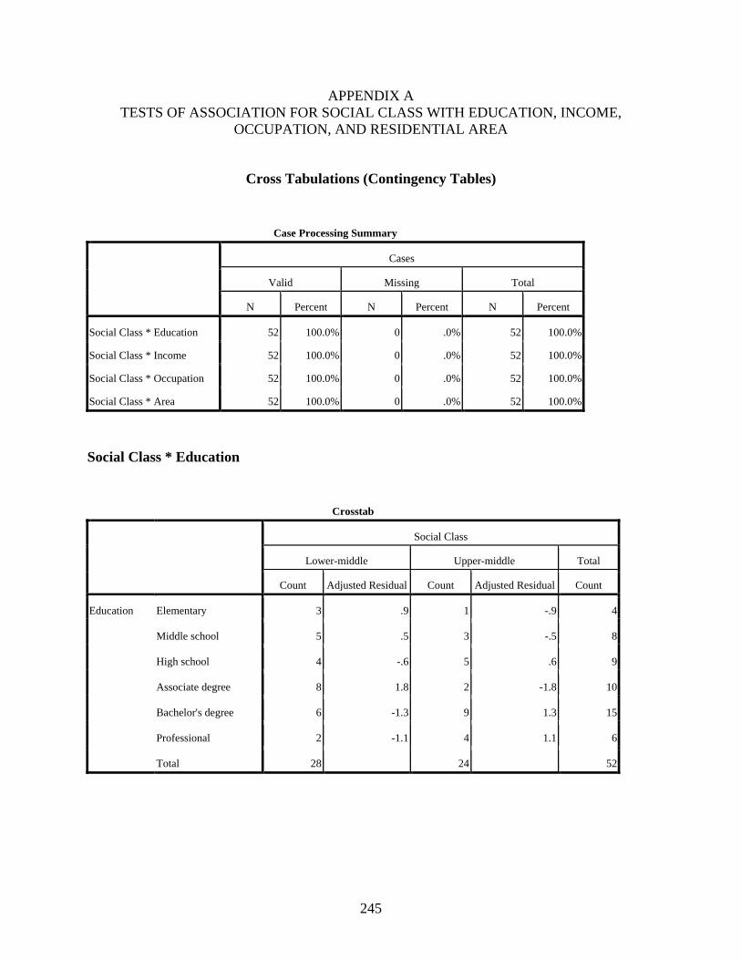
245
APPENDIX A TESTS OF ASSOCIATION FOR SOCIAL CLASS WITH EDUCATION, INCOME,
OCCUPATION, AND RESIDENTIAL AREA
Cross Tabulations (Contingency Tables)
Case Processing Summary
Cases
Valid Missing Total
N Percent N Percent N Percent
Social Class * Education 52 100.0% 0 .0% 52 100.0%
Social Class * Income 52 100.0% 0 .0% 52 100.0%
Social Class * Occupation 52 100.0% 0 .0% 52 100.0%
Social Class * Area 52 100.0% 0 .0% 52 100.0%
Social Class * Education
Crosstab
Social Class
Lower-middle Upper-middle Total
Count Adjusted Residual Count Adjusted Residual Count
Education Elementary 3 .9 1 -.9 4
Middle school 5 .5 3 -.5 8
High school 4 -.6 5 .6 9
Associate degree 8 1.8 2 -1.8 10
Bachelor's degree 6 -1.3 9 1.3 15
Professional 2 -1.1 4 1.1 6
Total 28 24 52
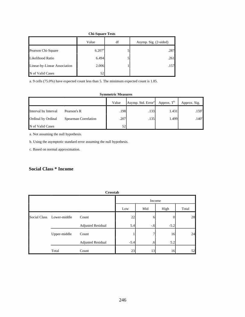
246
Chi-Square Tests
Value df Asymp. Sig. (2-sided)
Pearson Chi-Square 6.207a 5 .287
Likelihood Ratio 6.494 5 .261
Linear-by-Linear Association 2.006 1 .157
N of Valid Cases 52
a. 9 cells (75.0%) have expected count less than 5. The minimum expected count is 1.85.
Symmetric Measures
Value Asymp. Std. Errora Approx. Tb Approx. Sig.
Interval by Interval Pearson's R .198 .133 1.431 .159c
Ordinal by Ordinal Spearman Correlation .207 .135 1.499 .140c
N of Valid Cases 52
a. Not assuming the null hypothesis.
b. Using the asymptotic standard error assuming the null hypothesis.
c. Based on normal approximation.
Social Class * Income
Crosstab
Income
Low Mid High Total
Social Class Lower-middle Count 22 6 0 28
Adjusted Residual 5.4 -.6 -5.2
Upper-middle Count 1 7 16 24
Adjusted Residual -5.4 .6 5.2
Total Count 23 13 16 52
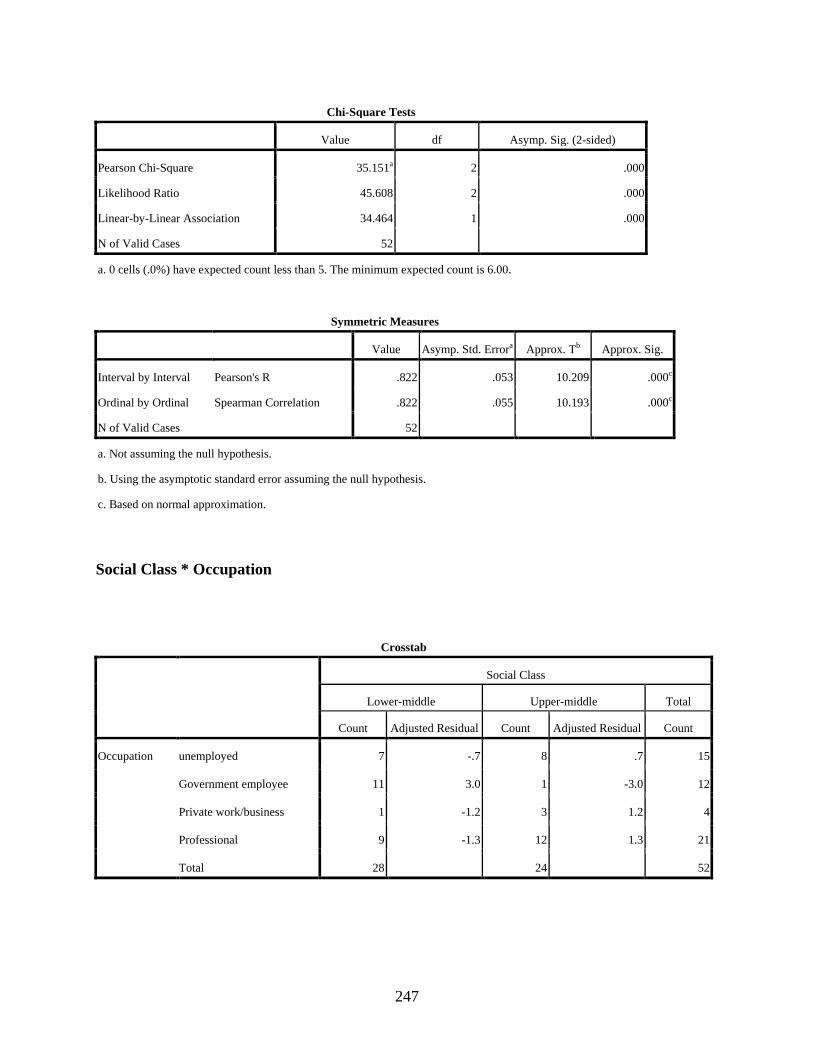
247
Chi-Square Tests
Value df Asymp. Sig. (2-sided)
Pearson Chi-Square 35.151a 2 .000
Likelihood Ratio 45.608 2 .000
Linear-by-Linear Association 34.464 1 .000
N of Valid Cases 52
a. 0 cells (.0%) have expected count less than 5. The minimum expected count is 6.00.
Symmetric Measures
Value Asymp. Std. Errora Approx. Tb Approx. Sig.
Interval by Interval Pearson's R .822 .053 10.209 .000c
Ordinal by Ordinal Spearman Correlation .822 .055 10.193 .000c
N of Valid Cases 52
a. Not assuming the null hypothesis.
b. Using the asymptotic standard error assuming the null hypothesis.
c. Based on normal approximation.
Social Class * Occupation
Crosstab
Social Class
Lower-middle Upper-middle Total
Count Adjusted Residual Count Adjusted Residual Count
Occupation unemployed 7 -.7 8 .7 15
Government employee 11 3.0 1 -3.0 12
Private work/business 1 -1.2 3 1.2 4
Professional 9 -1.3 12 1.3 21
Total 28 24 52
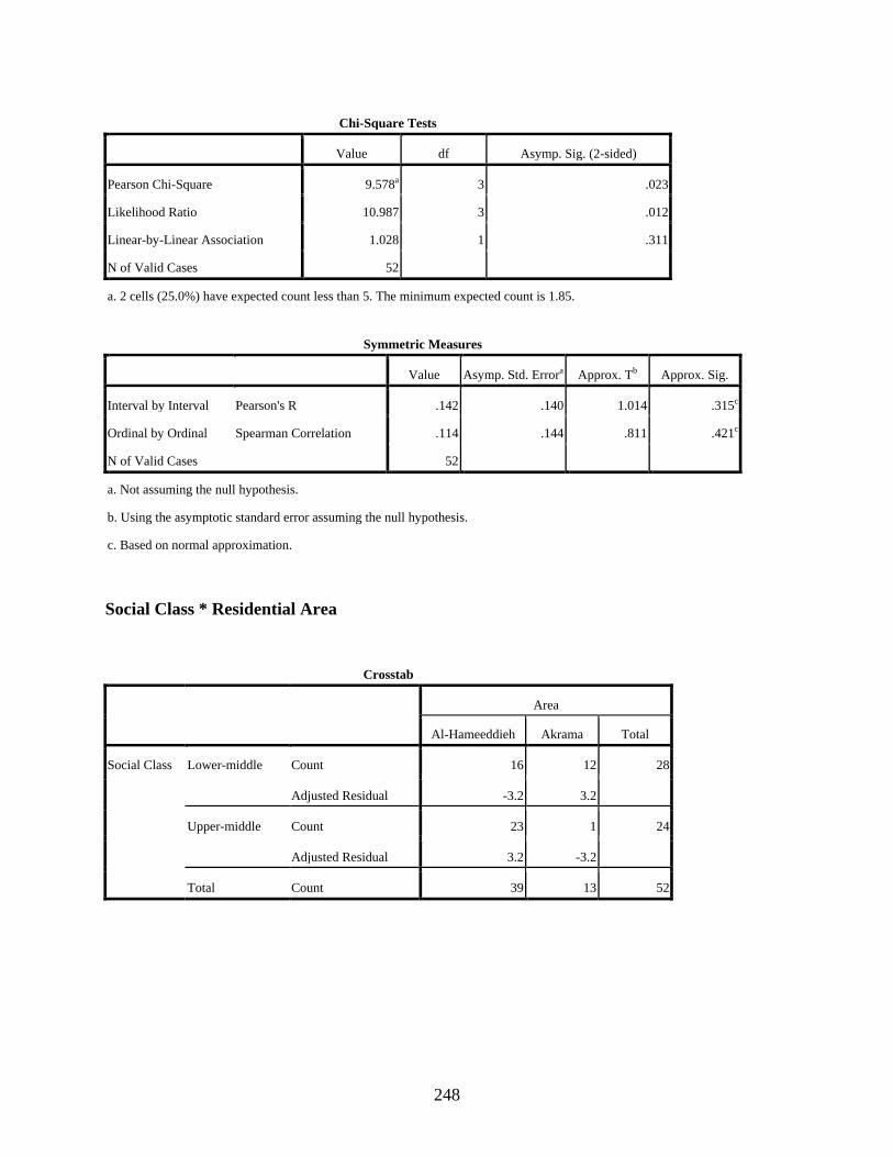
248
Chi-Square Tests
Value df Asymp. Sig. (2-sided)
Pearson Chi-Square 9.578a 3 .023
Likelihood Ratio 10.987 3 .012
Linear-by-Linear Association 1.028 1 .311
N of Valid Cases 52
a. 2 cells (25.0%) have expected count less than 5. The minimum expected count is 1.85.
Symmetric Measures
Value Asymp. Std. Errora Approx. Tb Approx. Sig.
Interval by Interval Pearson's R .142 .140 1.014 .315c
Ordinal by Ordinal Spearman Correlation .114 .144 .811 .421c
N of Valid Cases 52
a. Not assuming the null hypothesis.
b. Using the asymptotic standard error assuming the null hypothesis.
c. Based on normal approximation. Social Class * Residential Area
Crosstab
Area
Al-Hameeddieh Akrama Total
Social Class Lower-middle Count 16 12 28
Adjusted Residual -3.2 3.2
Upper-middle Count 23 1 24
Adjusted Residual 3.2 -3.2
Total Count 39 13 52
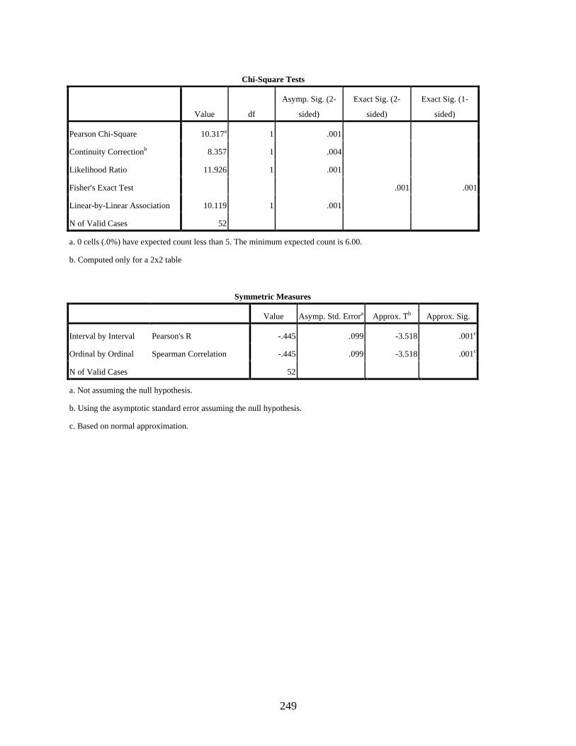
249
Chi-Square Tests
Value df
Asymp. Sig. (2-
sided)
Exact Sig. (2-
sided)
Exact Sig. (1-
sided)
Pearson Chi-Square 10.317a 1 .001
Continuity Correctionb 8.357 1 .004
Likelihood Ratio 11.926 1 .001
Fisher's Exact Test .001 .001
Linear-by-Linear Association 10.119 1 .001
N of Valid Cases 52
a. 0 cells (.0%) have expected count less than 5. The minimum expected count is 6.00.
b. Computed only for a 2x2 table
Symmetric Measures
Value Asymp. Std. Errora Approx. Tb Approx. Sig.
Interval by Interval Pearson's R -.445 .099 -3.518 .001c
Ordinal by Ordinal Spearman Correlation -.445 .099 -3.518 .001c
N of Valid Cases 52
a. Not assuming the null hypothesis.
b. Using the asymptotic standard error assuming the null hypothesis.
c. Based on normal approximation.
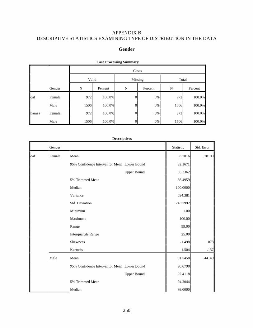
250
APPENDIX B DESCRIPTIVE STATISTICS EXAMINING TYPE OF DISTRIBUTION IN THE DATA
Gender
Case Processing Summary
Gender
Cases
Valid Missing Total
N Percent N Percent N Percent
qaf Female 972 100.0% 0 .0% 972 100.0%
Male 1506 100.0% 0 .0% 1506 100.0%
hamza Female 972 100.0% 0 .0% 972 100.0%
Male 1506 100.0% 0 .0% 1506 100.0%
Descriptives
Gender Statistic Std. Error
qaf Female Mean 83.7016 .78199
95% Confidence Interval for Mean Lower Bound 82.1671
Upper Bound 85.2362
5% Trimmed Mean 86.4959
Median 100.0000
Variance 594.381
Std. Deviation 24.37992
Minimum 1.00
Maximum 100.00
Range 99.00
Interquartile Range 25.00
Skewness -1.498 .078
Kurtosis 1.504 .157
Male Mean 91.5458 .44149
95% Confidence Interval for Mean Lower Bound 90.6798
Upper Bound 92.4118
5% Trimmed Mean 94.2044
Median 99.0000
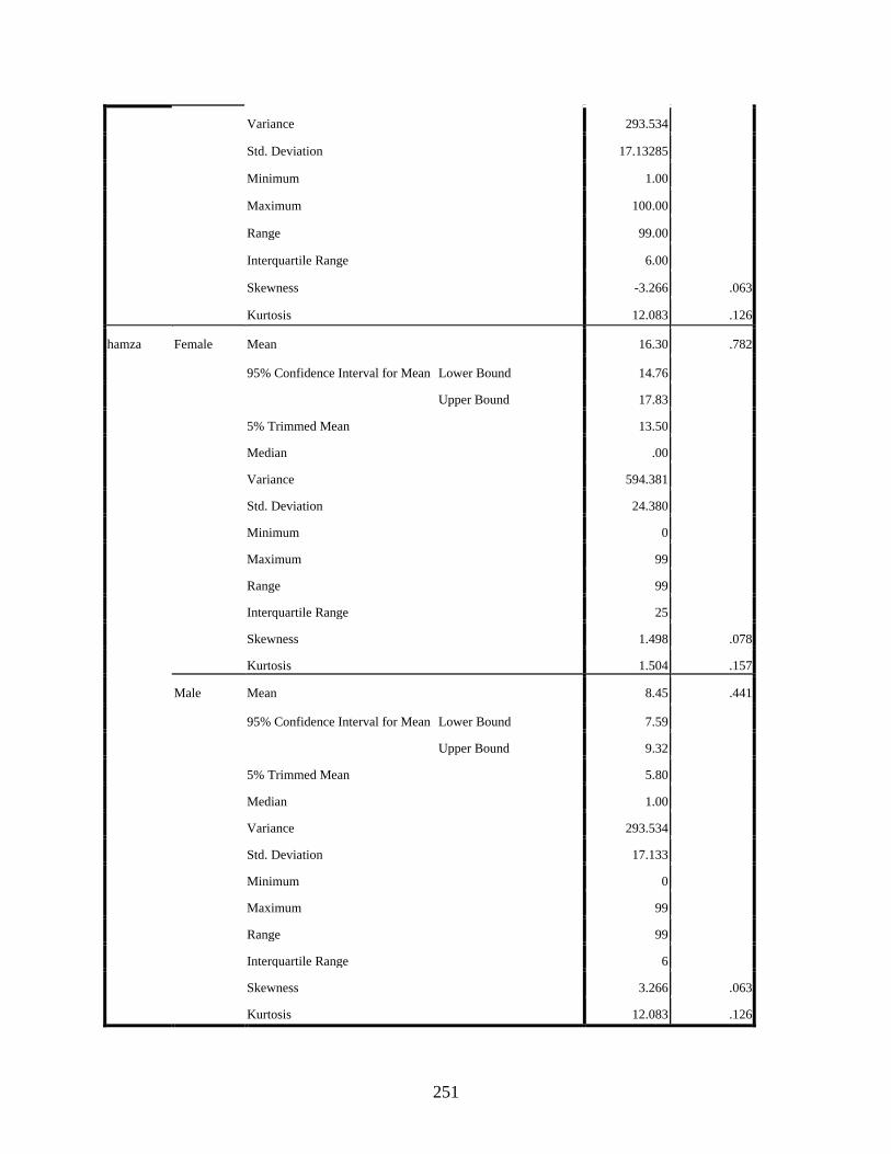
251
Variance 293.534
Std. Deviation 17.13285
Minimum 1.00
Maximum 100.00
Range 99.00
Interquartile Range 6.00
Skewness -3.266 .063
Kurtosis 12.083 .126
hamza Female Mean 16.30 .782
95% Confidence Interval for Mean Lower Bound 14.76
Upper Bound 17.83
5% Trimmed Mean 13.50
Median .00
Variance 594.381
Std. Deviation 24.380
Minimum 0
Maximum 99
Range 99
Interquartile Range 25
Skewness 1.498 .078
Kurtosis 1.504 .157
Male Mean 8.45 .441
95% Confidence Interval for Mean Lower Bound 7.59
Upper Bound 9.32
5% Trimmed Mean 5.80
Median 1.00
Variance 293.534
Std. Deviation 17.133
Minimum 0
Maximum 99
Range 99
Interquartile Range 6
Skewness 3.266 .063
Kurtosis 12.083 .126
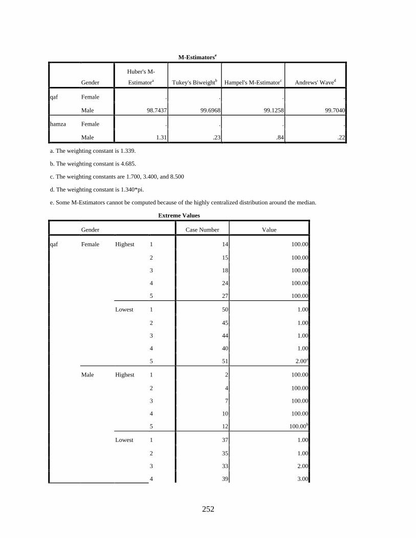
252
M-Estimatorse
Gender
Huber's M-
Estimatora Tukey's Biweightb Hampel's M-Estimatorc Andrews' Waved
qaf Female . . . .
Male 98.7437 99.6968 99.1258 99.7040
hamza Female . . . .
Male 1.31 .23 .84 .22
a. The weighting constant is 1.339.
b. The weighting constant is 4.685.
c. The weighting constants are 1.700, 3.400, and 8.500
d. The weighting constant is 1.340*pi.
e. Some M-Estimators cannot be computed because of the highly centralized distribution around the median.
Extreme Values
Gender Case Number Value
qaf Female Highest 1 14 100.00
2 15 100.00
3 18 100.00
4 24 100.00
5 27 100.00
Lowest 1 50 1.00
2 45 1.00
3 44 1.00
4 40 1.00
5 51 2.00a
Male Highest 1 2 100.00
2 4 100.00
3 7 100.00
4 10 100.00
5 12 100.00b
Lowest 1 37 1.00
2 35 1.00
3 33 2.00
4 39 3.00
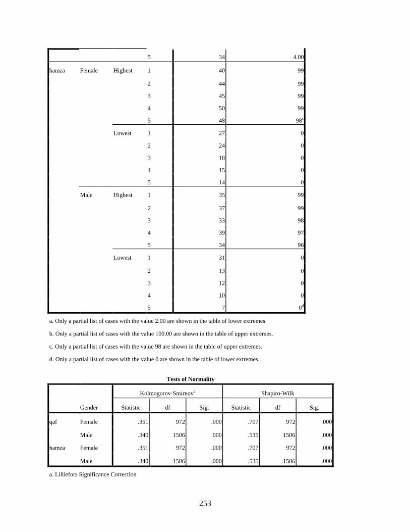
253
5 34 4.00
hamza Female Highest 1 40 99
2 44 99
3 45 99
4 50 99
5 48 98c
Lowest 1 27 0
2 24 0
3 18 0
4 15 0
5 14 0
Male Highest 1 35 99
2 37 99
3 33 98
4 39 97
5 34 96
Lowest 1 31 0
2 13 0
3 12 0
4 10 0
5 7 0d
a. Only a partial list of cases with the value 2.00 are shown in the table of lower extremes.
b. Only a partial list of cases with the value 100.00 are shown in the table of upper extremes.
c. Only a partial list of cases with the value 98 are shown in the table of upper extremes.
d. Only a partial list of cases with the value 0 are shown in the table of lower extremes.
Tests of Normality
Gender
Kolmogorov-Smirnova Shapiro-Wilk
Statistic df Sig. Statistic df Sig.
qaf Female .351 972 .000 .707 972 .000
Male .340 1506 .000 .535 1506 .000
hamza Female .351 972 .000 .707 972 .000
Male .340 1506 .000 .535 1506 .000
a. Lilliefors Significance Correction
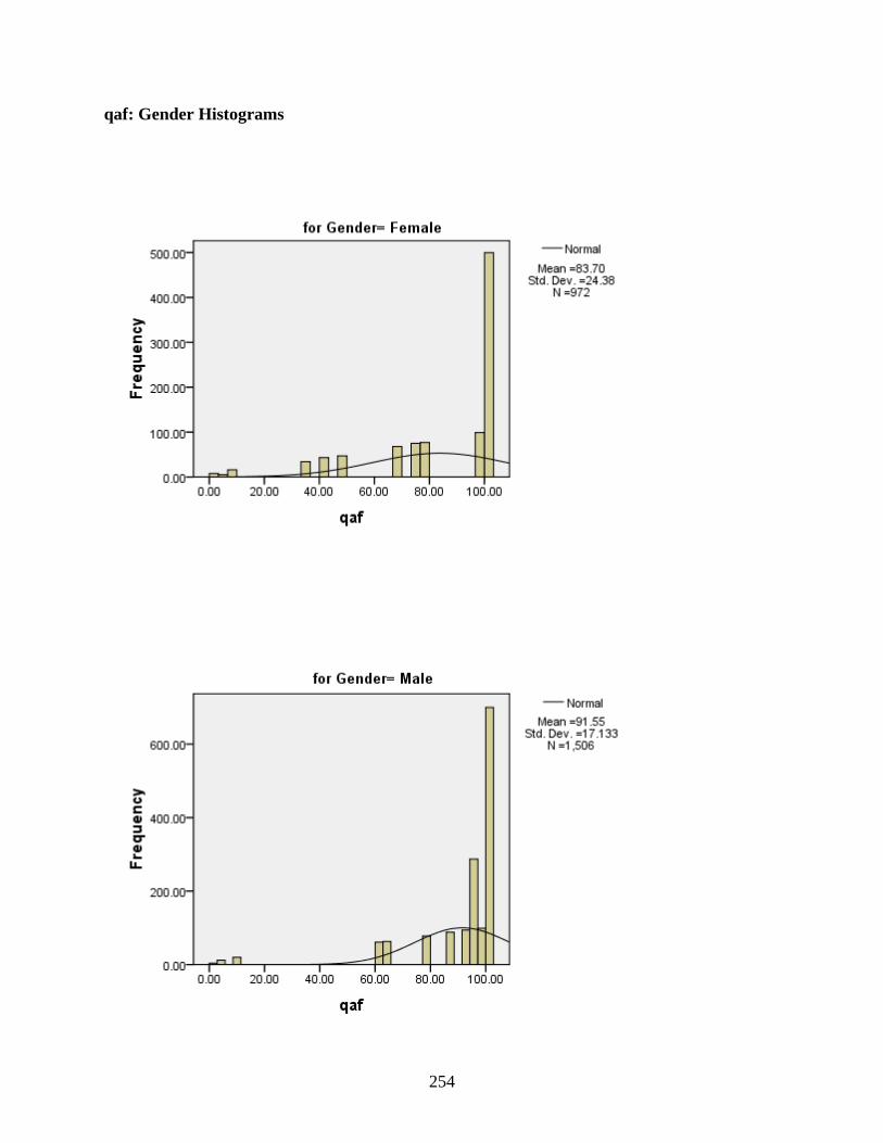
254
qaf: Gender Histograms

255
qaf: Gender Boxplots
hamza: Gender Histograms
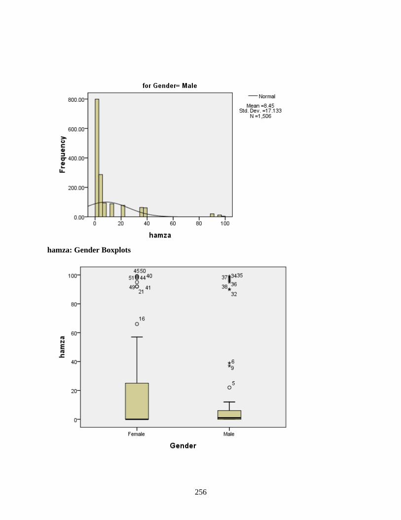
256
hamza: Gender Boxplots
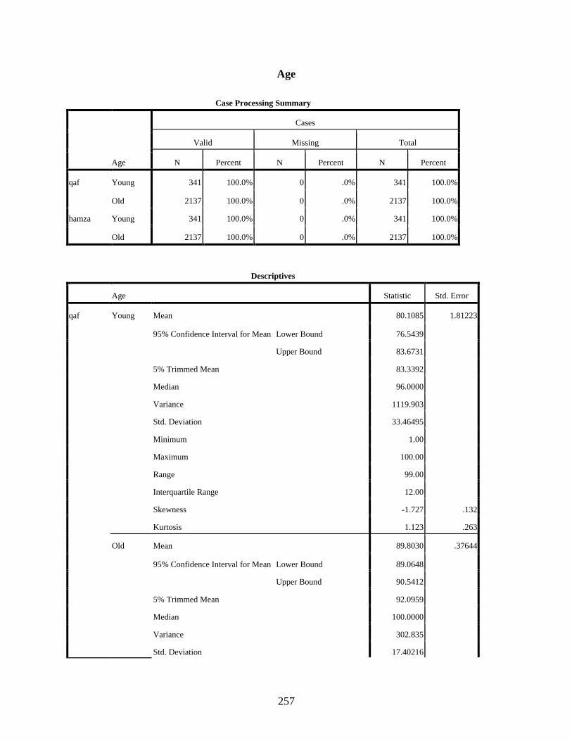
257
Age
Case Processing Summary
Age
Cases
Valid Missing Total
N Percent N Percent N Percent
qaf Young 341 100.0% 0 .0% 341 100.0%
Old 2137 100.0% 0 .0% 2137 100.0%
hamza Young 341 100.0% 0 .0% 341 100.0%
Old 2137 100.0% 0 .0% 2137 100.0%
Descriptives
Age Statistic Std. Error
qaf Young Mean 80.1085 1.81223
95% Confidence Interval for Mean Lower Bound 76.5439
Upper Bound 83.6731
5% Trimmed Mean 83.3392
Median 96.0000
Variance 1119.903
Std. Deviation 33.46495
Minimum 1.00
Maximum 100.00
Range 99.00
Interquartile Range 12.00
Skewness -1.727 .132
Kurtosis 1.123 .263
Old Mean 89.8030 .37644
95% Confidence Interval for Mean Lower Bound 89.0648
Upper Bound 90.5412
5% Trimmed Mean 92.0959
Median 100.0000
Variance 302.835
Std. Deviation 17.40216
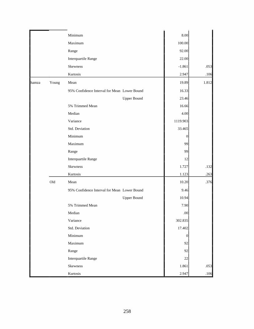
258
Minimum 8.00
Maximum 100.00
Range 92.00
Interquartile Range 22.00
Skewness -1.861 .053
Kurtosis 2.947 .106
hamza Young Mean 19.89 1.812
95% Confidence Interval for Mean Lower Bound 16.33
Upper Bound 23.46
5% Trimmed Mean 16.66
Median 4.00
Variance 1119.903
Std. Deviation 33.465
Minimum 0
Maximum 99
Range 99
Interquartile Range 12
Skewness 1.727 .132
Kurtosis 1.123 .263
Old Mean 10.20 .376
95% Confidence Interval for Mean Lower Bound 9.46
Upper Bound 10.94
5% Trimmed Mean 7.90
Median .00
Variance 302.835
Std. Deviation 17.402
Minimum 0
Maximum 92
Range 92
Interquartile Range 22
Skewness 1.861 .053
Kurtosis 2.947 .106

259
M-Estimatorse
Age
Huber's M-
Estimatora Tukey's Biweightb Hampel's M-Estimatorc Andrews' Waved
qaf Young 94.1673 95.5674 95.0705 95.5673
Old . . . .
hamza Young 6.46 4.60 5.00 4.60
Old . . . .
a. The weighting constant is 1.339.
b. The weighting constant is 4.685.
c. The weighting constants are 1.700, 3.400, and 8.500
d. The weighting constant is 1.340*pi.
e. Some M-Estimators cannot be computed because of the highly centralized distribution around the median.
Extreme Values
Age Case Number Value
qaf Young Highest 1 31 100.00
2 30 96.00
3 29 88.00
4 32 10.00
5 36 10.00
Lowest 1 50 1.00
2 45 1.00
3 44 1.00
4 40 1.00
5 37 1.00a
Old Highest 1 2 100.00
2 4 100.00
3 7 100.00
4 10 100.00
5 12 100.00b
Lowest 1 21 8.00
2 16 34.00
3 19 43.00
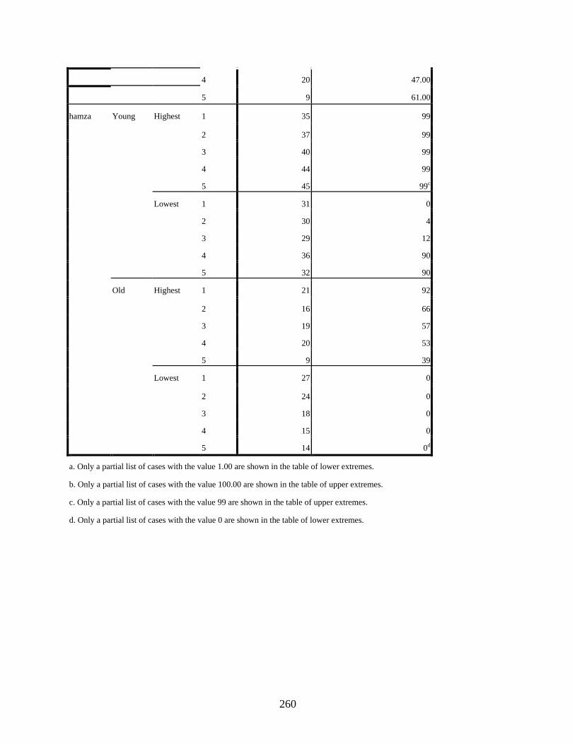
260
4 20 47.00
5 9 61.00
hamza Young Highest 1 35 99
2 37 99
3 40 99
4 44 99
5 45 99c
Lowest 1 31 0
2 30 4
3 29 12
4 36 90
5 32 90
Old Highest 1 21 92
2 16 66
3 19 57
4 20 53
5 9 39
Lowest 1 27 0
2 24 0
3 18 0
4 15 0
5 14 0d
a. Only a partial list of cases with the value 1.00 are shown in the table of lower extremes.
b. Only a partial list of cases with the value 100.00 are shown in the table of upper extremes.
c. Only a partial list of cases with the value 99 are shown in the table of upper extremes.
d. Only a partial list of cases with the value 0 are shown in the table of lower extremes.

261
Tests of Normality
Age
Kolmogorov-Smirnova Shapiro-Wilk
Statistic df Sig. Statistic df Sig.
qaf Young .426 341 .000 .569 341 .000
Old .336 2137 .000 .650 2137 .000
hamza Young .426 341 .000 .569 341 .000
Old .336 2137 .000 .650 2137 .000
a. Lilliefors Significance Correction
qaf: Age Histograms
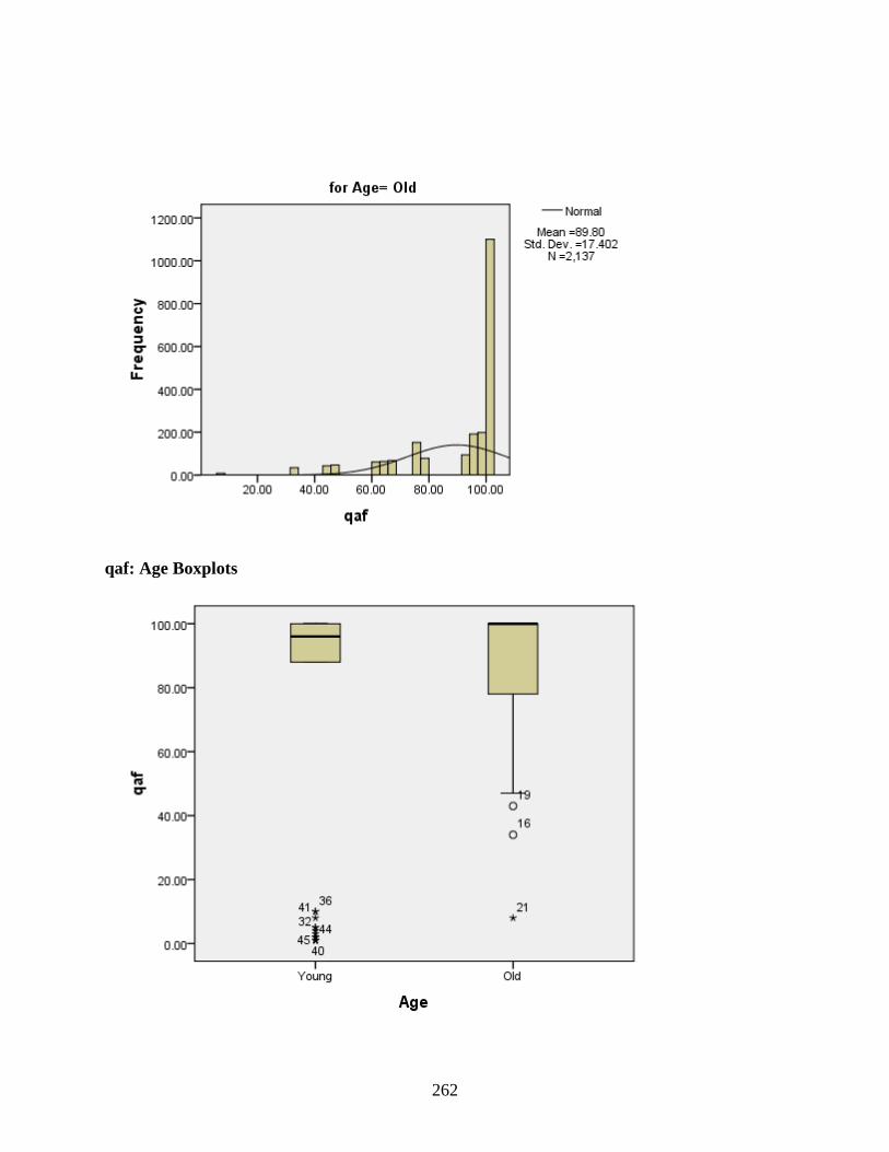
262
qaf: Age Boxplots
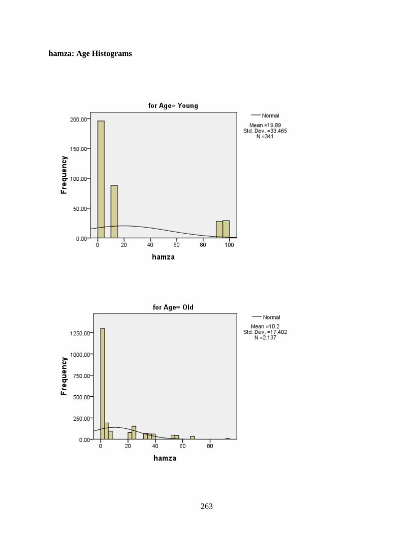
263
hamza: Age Histograms
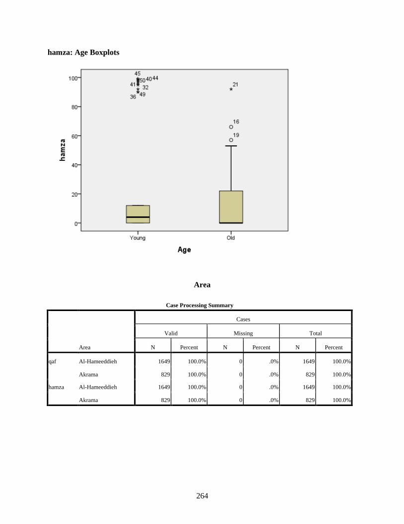
264
hamza: Age Boxplots
Area
Case Processing Summary
Area
Cases
Valid Missing Total
N Percent N Percent N Percent
qaf Al-Hameeddieh 1649 100.0% 0 .0% 1649 100.0%
Akrama 829 100.0% 0 .0% 829 100.0%
hamza Al-Hameeddieh 1649 100.0% 0 .0% 1649 100.0%
Akrama 829 100.0% 0 .0% 829 100.0%
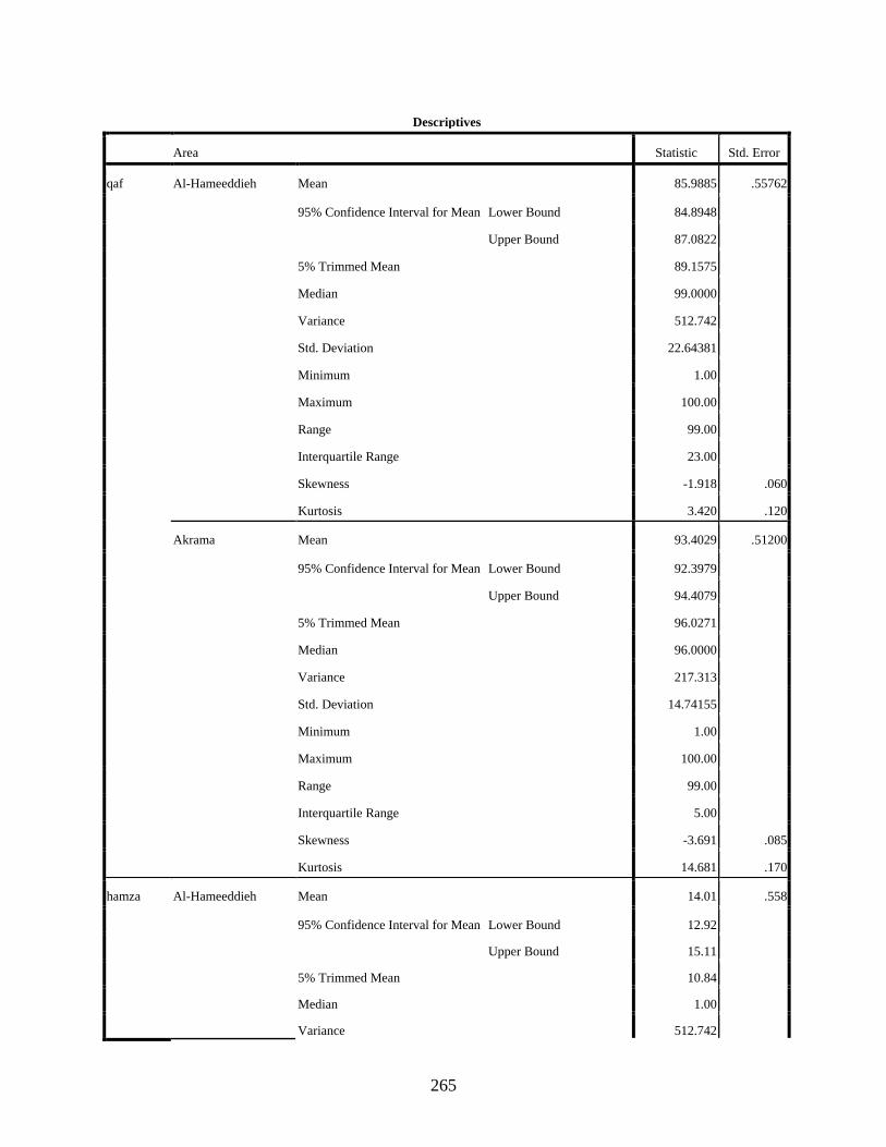
265
Descriptives
Area Statistic Std. Error
qaf Al-Hameeddieh Mean 85.9885 .55762
95% Confidence Interval for Mean Lower Bound 84.8948
Upper Bound 87.0822
5% Trimmed Mean 89.1575
Median 99.0000
Variance 512.742
Std. Deviation 22.64381
Minimum 1.00
Maximum 100.00
Range 99.00
Interquartile Range 23.00
Skewness -1.918 .060
Kurtosis 3.420 .120
Akrama Mean 93.4029 .51200
95% Confidence Interval for Mean Lower Bound 92.3979
Upper Bound 94.4079
5% Trimmed Mean 96.0271
Median 96.0000
Variance 217.313
Std. Deviation 14.74155
Minimum 1.00
Maximum 100.00
Range 99.00
Interquartile Range 5.00
Skewness -3.691 .085
Kurtosis 14.681 .170
hamza Al-Hameeddieh Mean 14.01 .558
95% Confidence Interval for Mean Lower Bound 12.92
Upper Bound 15.11
5% Trimmed Mean 10.84
Median 1.00
Variance 512.742
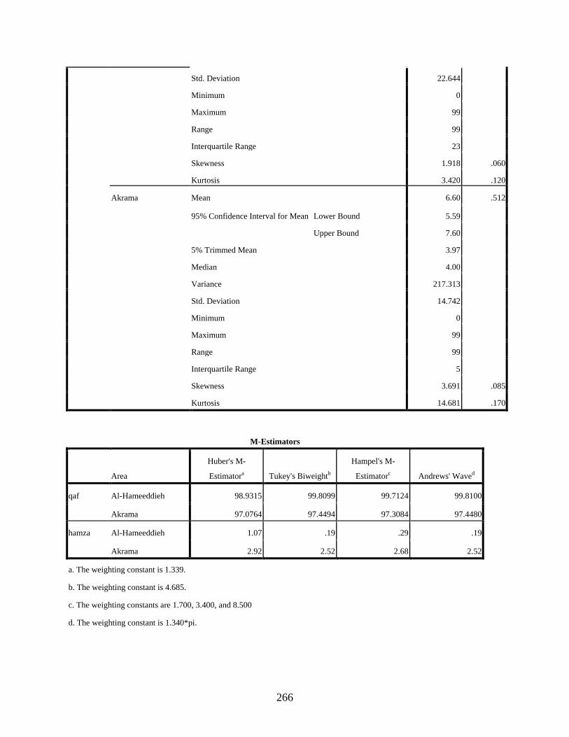
266
Std. Deviation 22.644
Minimum 0
Maximum 99
Range 99
Interquartile Range 23
Skewness 1.918 .060
Kurtosis 3.420 .120
Akrama Mean 6.60 .512
95% Confidence Interval for Mean Lower Bound 5.59
Upper Bound 7.60
5% Trimmed Mean 3.97
Median 4.00
Variance 217.313
Std. Deviation 14.742
Minimum 0
Maximum 99
Range 99
Interquartile Range 5
Skewness 3.691 .085
Kurtosis 14.681 .170
M-Estimators
Area
Huber's M-
Estimatora Tukey's Biweightb
Hampel's M-
Estimatorc Andrews' Waved
qaf Al-Hameeddieh 98.9315 99.8099 99.7124 99.8100
Akrama 97.0764 97.4494 97.3084 97.4480
hamza Al-Hameeddieh 1.07 .19 .29 .19
Akrama 2.92 2.52 2.68 2.52
a. The weighting constant is 1.339.
b. The weighting constant is 4.685.
c. The weighting constants are 1.700, 3.400, and 8.500
d. The weighting constant is 1.340*pi.
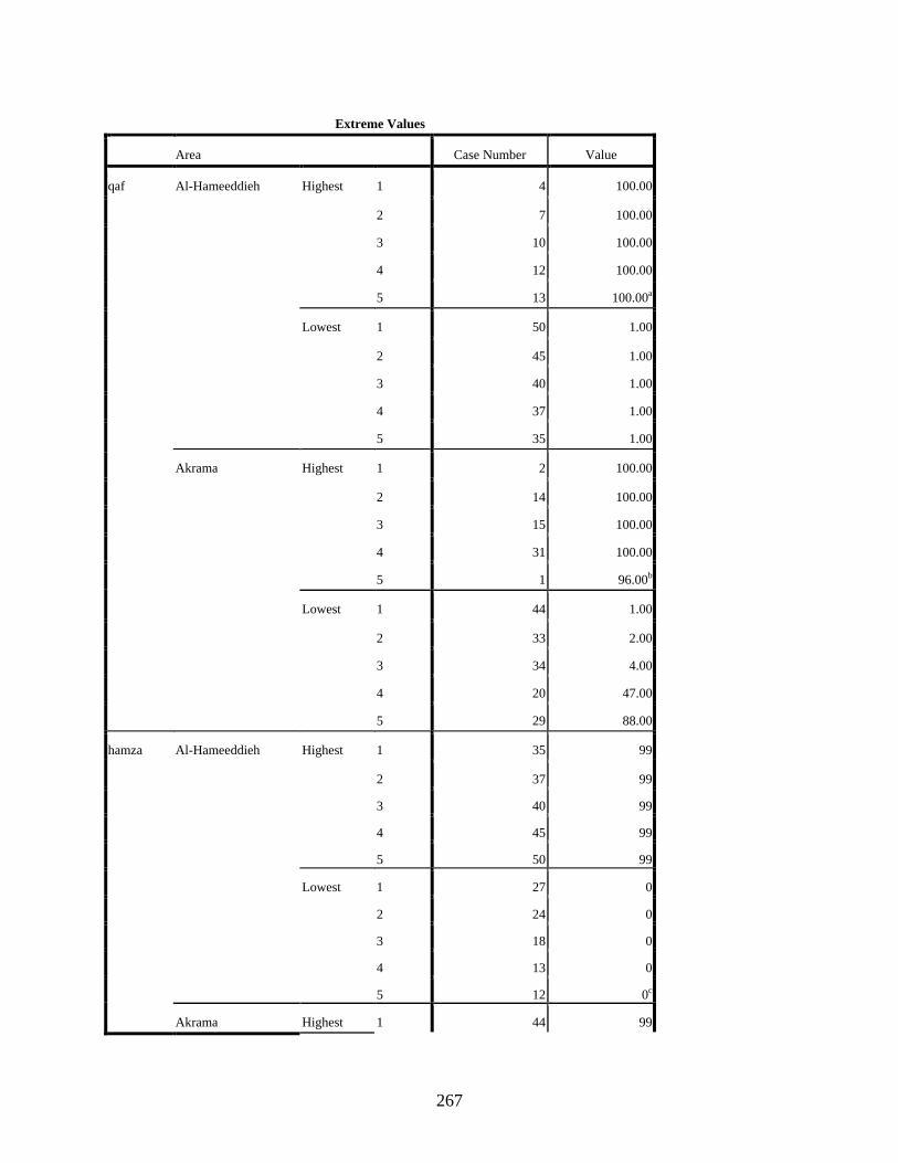
267
Extreme Values
Area Case Number Value
qaf Al-Hameeddieh Highest 1 4 100.00
2 7 100.00
3 10 100.00
4 12 100.00
5 13 100.00a
Lowest 1 50 1.00
2 45 1.00
3 40 1.00
4 37 1.00
5 35 1.00
Akrama Highest 1 2 100.00
2 14 100.00
3 15 100.00
4 31 100.00
5 1 96.00b
Lowest 1 44 1.00
2 33 2.00
3 34 4.00
4 20 47.00
5 29 88.00
hamza Al-Hameeddieh Highest 1 35 99
2 37 99
3 40 99
4 45 99
5 50 99
Lowest 1 27 0
2 24 0
3 18 0
4 13 0
5 12 0c
Akrama Highest 1 44 99

268
2 33 98
3 34 96
4 20 53
5 29 12
Lowest 1 31 0
2 15 0
3 14 0
4 2 0
5 30 4d
a. Only a partial list of cases with the value 100.00 are shown in the table of upper extremes.
b. Only a partial list of cases with the value 96.00 are shown in the table of upper extremes.
c. Only a partial list of cases with the value 0 are shown in the table of lower extremes.
d. Only a partial list of cases with the value 4 are shown in the table of lower extremes.
Tests of Normality
Area
Kolmogorov-Smirnova Shapiro-Wilk
Statistic df Sig. Statistic df Sig.
qaf Al-Hameeddieh .322 1649 .000 .672 1649 .000
Akrama .372 829 .000 .455 829 .000
hamza Al-Hameeddieh .322 1649 .000 .672 1649 .000
Akrama .372 829 .000 .455 829 .000
a. Lilliefors Significance Correction
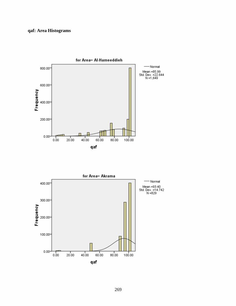
269
qaf: Area Histograms
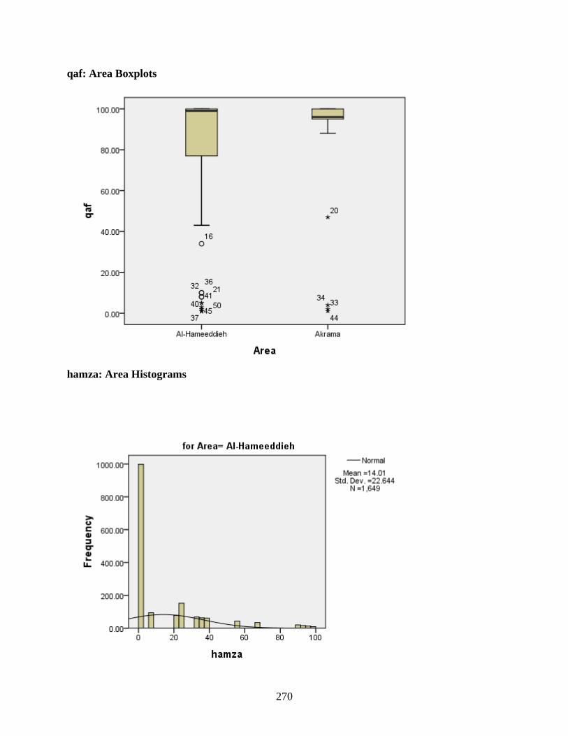
270
qaf: Area Boxplots
hamza: Area Histograms

271
hamza: Area Boxplots
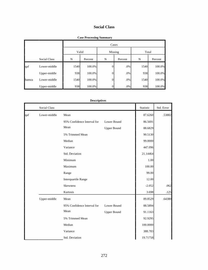
272
Social Class
Case Processing Summary
Social Class
Cases
Valid Missing Total
N Percent N Percent N Percent
qaf Lower-middle 1540 100.0% 0 .0% 1540 100.0%
Upper-middle 938 100.0% 0 .0% 938 100.0%
hamza Lower-middle 1540 100.0% 0 .0% 1540 100.0%
Upper-middle 938 100.0% 0 .0% 938 100.0%
Descriptives
Social Class Statistic Std. Error
qaf Lower-middle Mean 87.6260 .53882
95% Confidence Interval for
Mean
Lower Bound 86.5691
Upper Bound 88.6829
5% Trimmed Mean 90.5130
Median 99.0000
Variance 447.096
Std. Deviation 21.14464
Minimum 1.00
Maximum 100.00
Range 99.00
Interquartile Range 12.00
Skewness -2.052 .062
Kurtosis 3.698 .125
Upper-middle Mean 89.8529 .64380
95% Confidence Interval for
Mean
Lower Bound 88.5894
Upper Bound 91.1163
5% Trimmed Mean 92.9295
Median 100.0000
Variance 388.783
Std. Deviation 19.71758
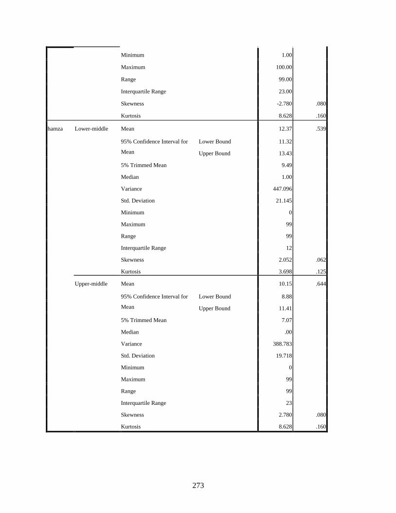
273
Minimum 1.00
Maximum 100.00
Range 99.00
Interquartile Range 23.00
Skewness -2.780 .080
Kurtosis 8.628 .160
hamza Lower-middle Mean 12.37 .539
95% Confidence Interval for
Mean
Lower Bound 11.32
Upper Bound 13.43
5% Trimmed Mean 9.49
Median 1.00
Variance 447.096
Std. Deviation 21.145
Minimum 0
Maximum 99
Range 99
Interquartile Range 12
Skewness 2.052 .062
Kurtosis 3.698 .125
Upper-middle Mean 10.15 .644
95% Confidence Interval for
Mean
Lower Bound 8.88
Upper Bound 11.41
5% Trimmed Mean 7.07
Median .00
Variance 388.783
Std. Deviation 19.718
Minimum 0
Maximum 99
Range 99
Interquartile Range 23
Skewness 2.780 .080
Kurtosis 8.628 .160
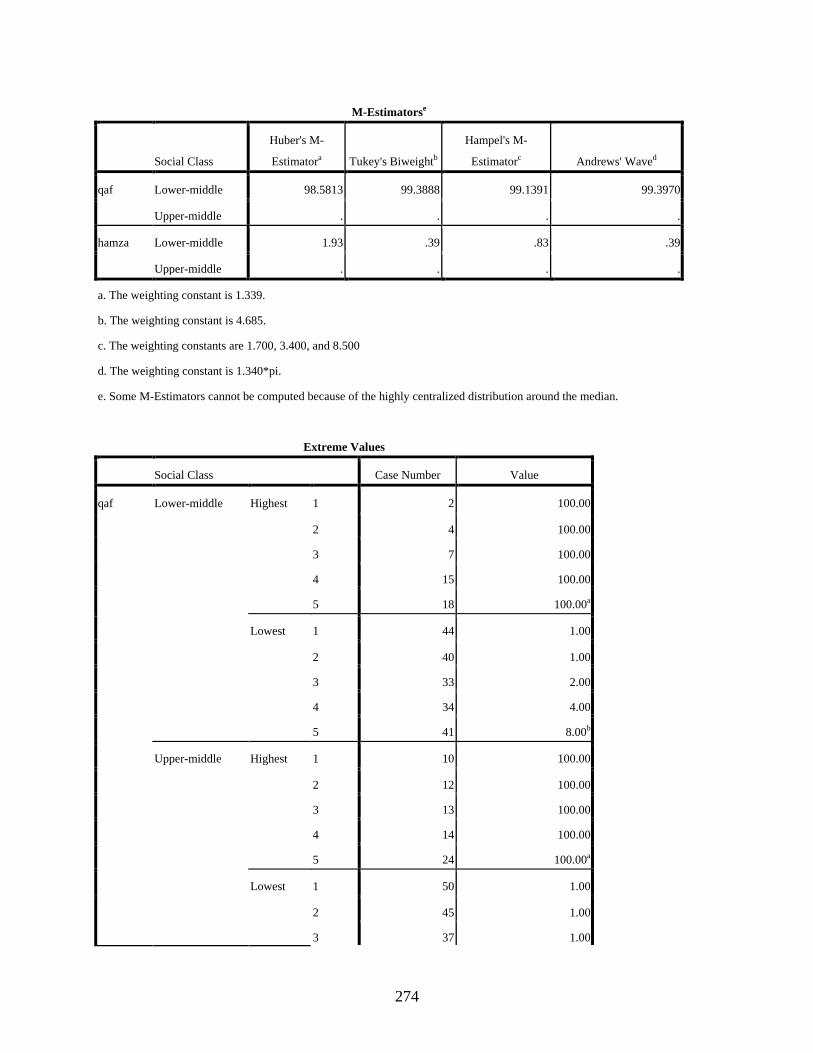
274
M-Estimatorse
Social Class
Huber's M-
Estimatora Tukey's Biweightb
Hampel's M-
Estimatorc Andrews' Waved
qaf Lower-middle 98.5813 99.3888 99.1391 99.3970
Upper-middle . . . .
hamza Lower-middle 1.93 .39 .83 .39
Upper-middle . . . .
a. The weighting constant is 1.339.
b. The weighting constant is 4.685.
c. The weighting constants are 1.700, 3.400, and 8.500
d. The weighting constant is 1.340*pi.
e. Some M-Estimators cannot be computed because of the highly centralized distribution around the median.
Extreme Values
Social Class Case Number Value
qaf Lower-middle Highest 1 2 100.00
2 4 100.00
3 7 100.00
4 15 100.00
5 18 100.00a
Lowest 1 44 1.00
2 40 1.00
3 33 2.00
4 34 4.00
5 41 8.00b
Upper-middle Highest 1 10 100.00
2 12 100.00
3 13 100.00
4 14 100.00
5 24 100.00a
Lowest 1 50 1.00
2 45 1.00
3 37 1.00
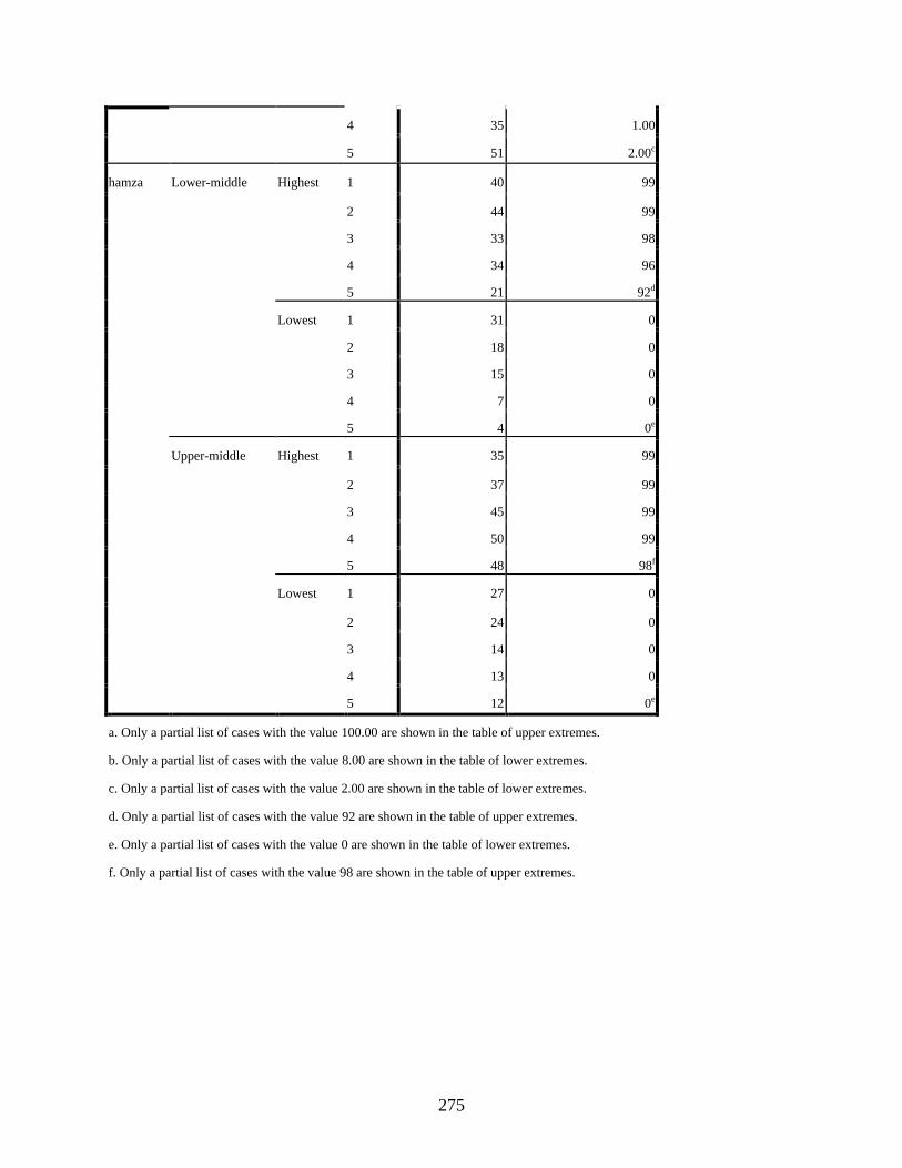
275
4 35 1.00
5 51 2.00c
hamza Lower-middle Highest 1 40 99
2 44 99
3 33 98
4 34 96
5 21 92d
Lowest 1 31 0
2 18 0
3 15 0
4 7 0
5 4 0e
Upper-middle Highest 1 35 99
2 37 99
3 45 99
4 50 99
5 48 98f
Lowest 1 27 0
2 24 0
3 14 0
4 13 0
5 12 0e
a. Only a partial list of cases with the value 100.00 are shown in the table of upper extremes.
b. Only a partial list of cases with the value 8.00 are shown in the table of lower extremes.
c. Only a partial list of cases with the value 2.00 are shown in the table of lower extremes.
d. Only a partial list of cases with the value 92 are shown in the table of upper extremes.
e. Only a partial list of cases with the value 0 are shown in the table of lower extremes.
f. Only a partial list of cases with the value 98 are shown in the table of upper extremes.
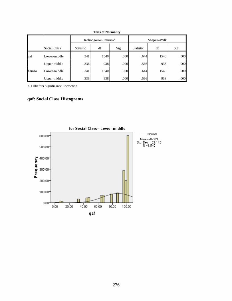
276
Tests of Normality
Social Class
Kolmogorov-Smirnova Shapiro-Wilk
Statistic df Sig. Statistic df Sig.
qaf Lower-middle .341 1540 .000 .644 1540 .000
Upper-middle .336 938 .000 .566 938 .000
hamza Lower-middle .341 1540 .000 .644 1540 .000
Upper-middle .336 938 .000 .566 938 .000
a. Lilliefors Significance Correction
qaf: Social Class Histograms
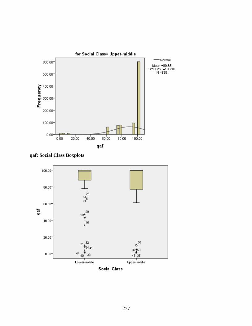
277
qaf: Social Class Boxplots
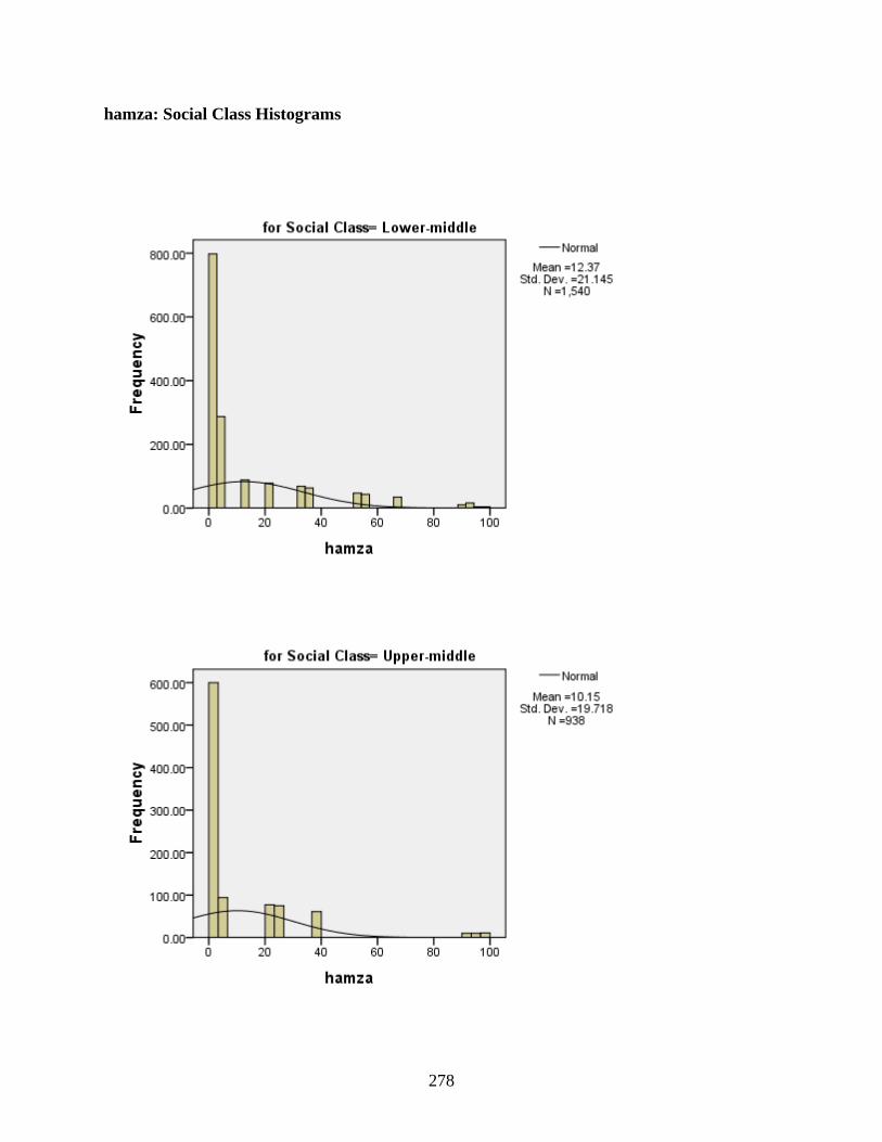
278
hamza: Social Class Histograms

279
hamza: Social Class Boxplots
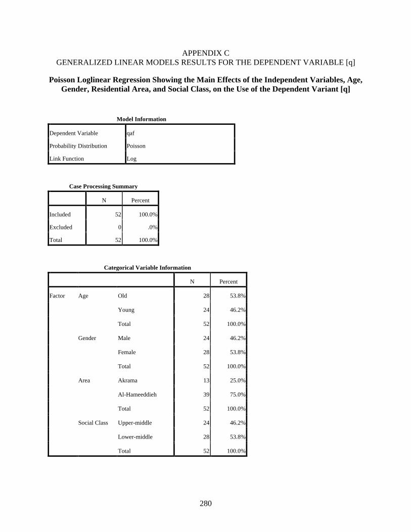
280
APPENDIX C GENERALIZED LINEAR MODELS RESULTS FOR THE DEPENDENT VARIABLE [q]
Poisson Loglinear Regression Showing the Main Effects of the Independent Variables, Age, Gender, Residential Area, and Social Class, on the Use of the Dependent Variant [q]
Model Information
Dependent Variable qaf
Probability Distribution Poisson
Link Function Log
Case Processing Summary
N Percent
Included 52 100.0%
Excluded 0 .0%
Total 52 100.0%
Categorical Variable Information
N Percent
Factor Age Old 28 53.8%
Young 24 46.2%
Total 52 100.0%
Gender Male 24 46.2%
Female 28 53.8%
Total 52 100.0%
Area Akrama 13 25.0%
Al-Hameeddieh 39 75.0%
Total 52 100.0%
Social Class Upper-middle 24 46.2%
Lower-middle 28 53.8%
Total 52 100.0%

281
Continuous Variable Information
N Minimum Maximum Mean Std. Deviation
Dependent Variable qaf 52 0 467 112.96 132.696
Goodness of Fitd
Value df Value/df
Deviance 4798.992 47 102.106
Scaled Deviance 39.659 47
Pearson Chi-Square 5687.238 47 121.005
Scaled Pearson Chi-Square 47.000 47
Log Likelihooda -2527.807
Adjusted Log Likelihoodc -20.890
Akaike's Information Criterion (AIC) 5065.613
Finite Sample Corrected AIC (AICC) 5066.918
Bayesian Information Criterion (BIC) 5075.369
Consistent AIC (CAIC) 5080.369
Dependent Variable: qaf
Model: (Intercept), Age, Gender, Area, Social Class
a. The full log likelihood function is displayed and used in computing information criteria.
c. The adjusted log likelihood is based on an estimated scale parameter and is used in the
model fitting omnibus test.
d. Information criteria are in small-is-better form.
Omnibus Testa
Likelihood Ratio
Chi-Square Df Sig.
28.042 4 .000
Dependent Variable: qaf
Model: (Intercept), Age, Gender, Area, Social Class
a. Compares the fitted model against the intercept-only model.
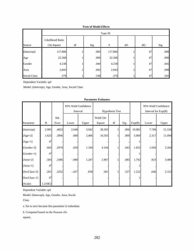
282
Tests of Model Effects
Source
Type III
Likelihood Ratio
Chi-Square df Sig. F df1 df2 Sig.
(Intercept) 117.806 1 .000 117.806 1 47 .000
Age 22.268 1 .000 22.268 1 47 .000
Gender 4.238 1 .040 4.238 1 47 .045
Area 2.843 1 .092 2.843 1 47 .098
Social Class .379 1 .538 .379 1 47 .541
Dependent Variable: qaf
Model: (Intercept), Age, Gender, Area, Social Class
Parameter Estimates
Parameter B
Std.
Error
95% Wald Confidence
Interval Hypothesis Test
Exp(B)
95% Wald Confidence
Interval for Exp(B)
Lower Upper
Wald Chi-
Square df Sig. Lower Upper
(Intercept) 2.995 .4833 2.048 3.942 38.393 1 .000 19.982 7.749 51.530
[Age=2] 1.623 .3996 .840 2.406 16.503 1 .000 5.069 2.317 11.094
[Age=1] 0a . . . . . . 1 . .
[Gender=2] .602 .2970 .020 1.184 4.104 1 .043 1.825 1.020 3.266
[Gender=1] 0a . . . . . . 1 . .
[Area=2] .583 .3386 -.080 1.247 2.967 1 .085 1.792 .923 3.480
[Area=1] 0a . . . . . . 1 . .
[SocClass=2] .201 .3252 -.437 .838 .381 1 .537 1.222 .646 2.312
[SocClass=1] 0a . . . . . . 1 . .
(Scale) 1.210E2
Dependent Variable: qaf
Model: (Intercept), Age, Gender, Area, Social
Class
a. Set to zero because this parameter is redundant.
b. Computed based on the Pearson chi-
square.
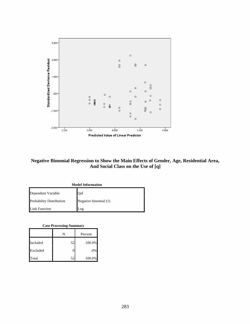
283
Negative Binomial Regression to Show the Main Effects of Gender, Age, Residential Area, And Social Class on the Use of [q]
Model Information
Dependent Variable Qaf
Probability Distribution Negative binomial (1)
Link Function Log
Case Processing Summary
N Percent
Included 52 100.0%
Excluded 0 .0%
Total 52 100.0%

284
Categorical Variable Information
N Percent
Factor Age Old 28 53.8%
Young 24 46.2%
Total 52 100.0%
Gender Male 24 46.2%
Female 28 53.8%
Total 52 100.0%
Area Akrama 13 25.0%
Al-Hameeddieh 39 75.0%
Total 52 100.0%
Social Class Upper-middle 24 46.2%
Lower-middle 28 53.8%
Total 52 100.0%
Continuous Variable Information
N Minimum Maximum Mean Std. Deviation
Dependent Variable qaf 52 0 467 112.96 132.696
Goodness of Fitd
Value df Value/df
Deviance 90.806 47 1.932
Scaled Deviance 56.837 47
Pearson Chi-Square 75.090 47 1.598
Scaled Pearson Chi-Square 47.000 47
Log Likelihooda -265.034
Adjusted Log Likelihoodc -165.890
Akaike's Information Criterion (AIC) 540.068
Finite Sample Corrected AIC (AICC) 541.373
Bayesian Information Criterion (BIC) 549.825
Consistent AIC (CAIC) 554.825
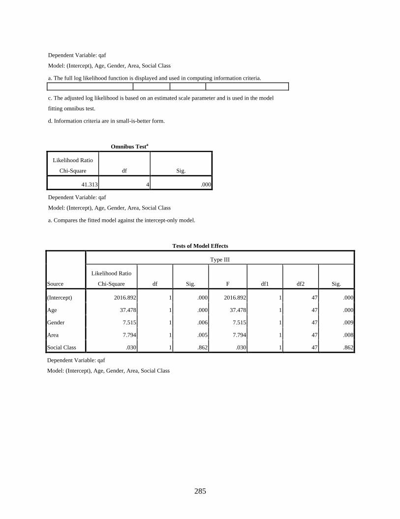
285
Dependent Variable: qaf
Model: (Intercept), Age, Gender, Area, Social Class
a. The full log likelihood function is displayed and used in computing information criteria.
c. The adjusted log likelihood is based on an estimated scale parameter and is used in the model
fitting omnibus test.
d. Information criteria are in small-is-better form.
Omnibus Testa
Likelihood Ratio
Chi-Square df Sig.
41.313 4 .000
Dependent Variable: qaf
Model: (Intercept), Age, Gender, Area, Social Class
a. Compares the fitted model against the intercept-only model.
Tests of Model Effects
Source
Type III
Likelihood Ratio
Chi-Square df Sig. F df1 df2 Sig.
(Intercept) 2016.892 1 .000 2016.892 1 47 .000
Age 37.478 1 .000 37.478 1 47 .000
Gender 7.515 1 .006 7.515 1 47 .009
Area 7.794 1 .005 7.794 1 47 .008
Social Class .030 1 .862 .030 1 47 .862
Dependent Variable: qaf
Model: (Intercept), Age, Gender, Area, Social Class
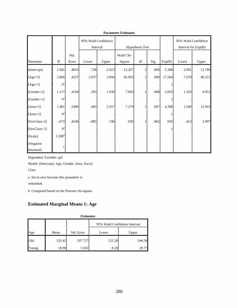
286
Parameter Estimates
Parameter B
Std.
Error
95% Wald Confidence
Interval Hypothesis Test
Exp(B)
95% Wald Confidence
Interval for Exp(B)
Lower Upper
Wald Chi-
Square df Sig. Lower Upper
(Intercept) 1.681 .4810 .738 2.623 12.207 1 .000 5.368 2.091 13.780
[Age=2] 2.866 .4227 2.037 3.694 45.963 1 .000 17.564 7.670 40.221
[Age=1] 0a . . . . . . 1 . .
[Gender=2] 1.117 .4194 .295 1.939 7.093 1 .008 3.055 1.343 6.951
[Gender=1] 0a . . . . . . 1 . .
[Area=2] 1.481 .5490 .405 2.557 7.279 1 .007 4.398 1.500 12.901
[Area=1] 0a . . . . . . 1 . .
[SocClass=2] -.072 .4146 -.885 .740 .030 1 .862 .930 .413 2.097
[SocClass=1] 0a . . . . . . 1 . .
(Scale) 1.598b
(Negative
binomial) 1
Dependent Variable: qaf
Model: (Intercept), Age, Gender, Area, Social
Class
a. Set to zero because this parameter is
redundant.
b. Computed based on the Pearson chi-square.
Estimated Marginal Means 1: Age
Estimates
Age Mean Std. Error
95% Wald Confidence Interval
Lower Upper
Old 333.42 107.727 122.28 544.56
Young 18.98 5.502 8.20 29.77
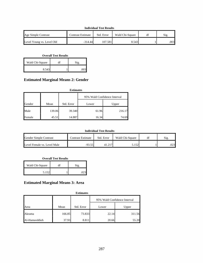
287
Individual Test Results
Age Simple Contrast Contrast Estimate Std. Error Wald Chi-Square df Sig.
Level Young vs. Level Old -314.44 107.581 8.543 1 .003
Overall Test Results
Wald Chi-Square df Sig.
8.543 1 .003
Estimated Marginal Means 2: Gender
Estimates
Gender Mean Std. Error
95% Wald Confidence Interval
Lower Upper
Male 139.06 39.340 61.96 216.17
Female 45.51 14.887 16.34 74.69
Individual Test Results
Gender Simple Contrast Contrast Estimate Std. Error Wald Chi-Square df Sig.
Level Female vs. Level Male -93.55 41.217 5.152 1 .023
Overall Test Results
Wald Chi-Square df Sig.
5.152 1 .023
Estimated Marginal Means 3: Area
Estimates
Area Mean Std. Error
95% Wald Confidence Interval
Lower Upper
Akrama 166.85 73.833 22.14 311.56
Al-Hameeddieh 37.93 8.811 20.66 55.20
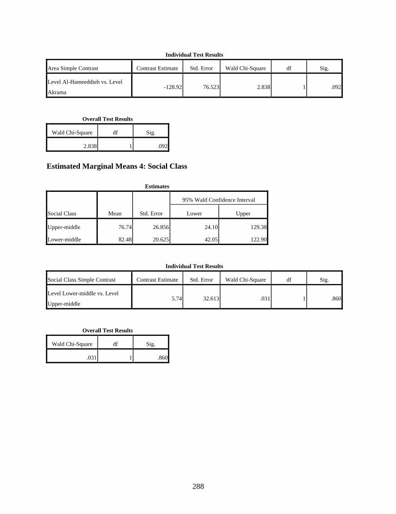
288
Individual Test Results
Area Simple Contrast Contrast Estimate Std. Error Wald Chi-Square df Sig.
Level Al-Hameeddieh vs. Level
Akrama -128.92 76.523 2.838 1 .092
Overall Test Results
Wald Chi-Square df Sig.
2.838 1 .092
Estimated Marginal Means 4: Social Class
Estimates
Social Class Mean Std. Error
95% Wald Confidence Interval
Lower Upper
Upper-middle 76.74 26.856 24.10 129.38
Lower-middle 82.48 20.625 42.05 122.90
Individual Test Results
Social Class Simple Contrast Contrast Estimate Std. Error Wald Chi-Square df Sig.
Level Lower-middle vs. Level
Upper-middle 5.74 32.613 .031 1 .860
Overall Test Results
Wald Chi-Square df Sig.
.031 1 .860
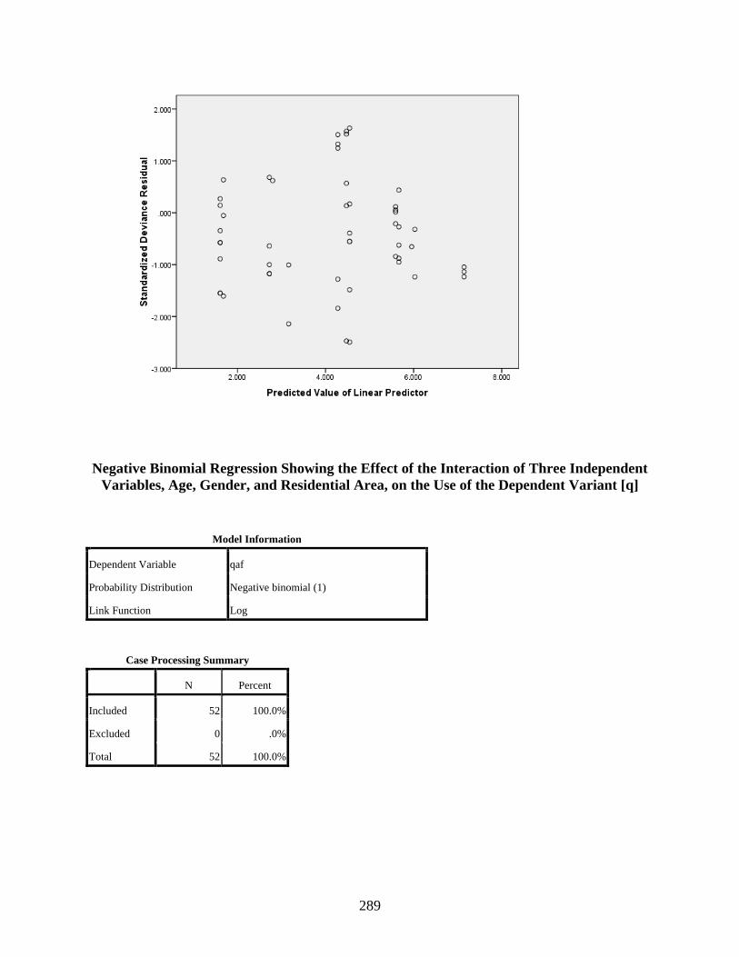
289
Negative Binomial Regression Showing the Effect of the Interaction of Three Independent Variables, Age, Gender, and Residential Area, on the Use of the Dependent Variant [q]
Model Information
Dependent Variable qaf
Probability Distribution Negative binomial (1)
Link Function Log
Case Processing Summary
N Percent
Included 52 100.0%
Excluded 0 .0%
Total 52 100.0%
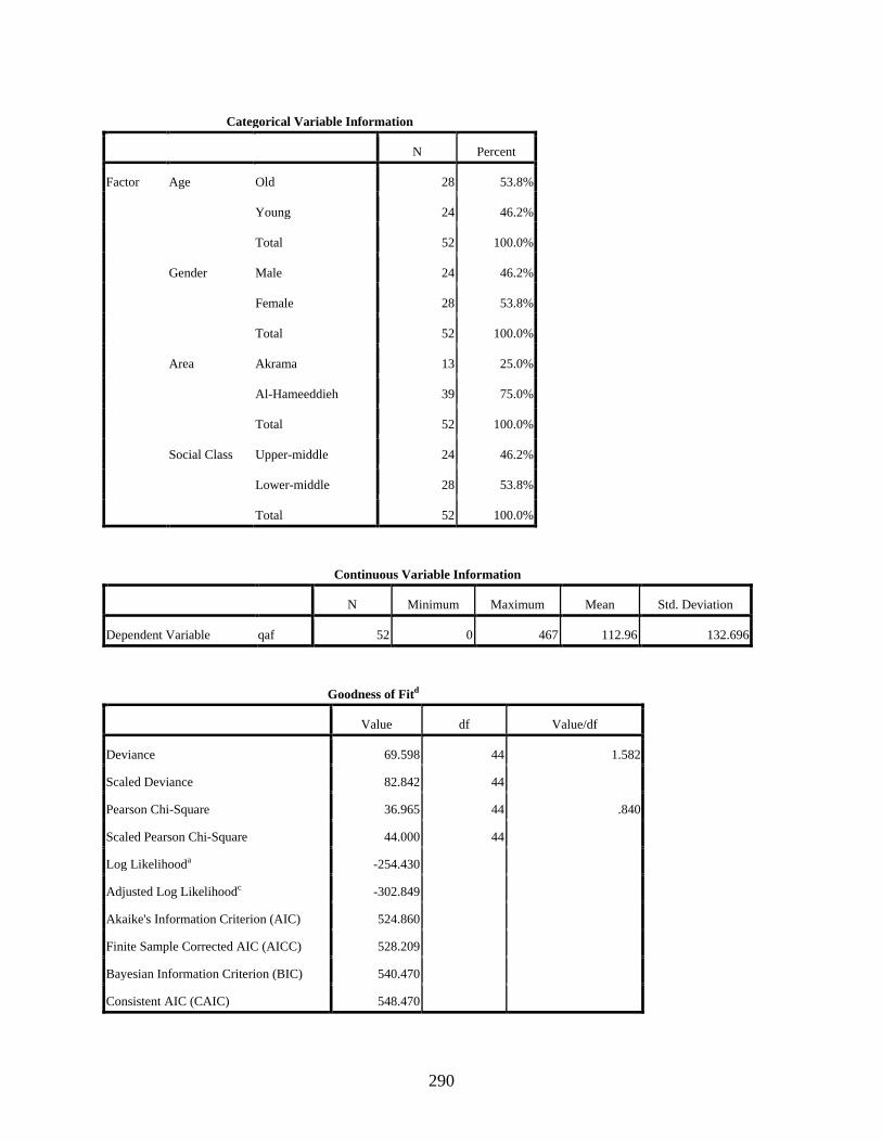
290
Categorical Variable Information
N Percent
Factor Age Old 28 53.8%
Young 24 46.2%
Total 52 100.0%
Gender Male 24 46.2%
Female 28 53.8%
Total 52 100.0%
Area Akrama 13 25.0%
Al-Hameeddieh 39 75.0%
Total 52 100.0%
Social Class Upper-middle 24 46.2%
Lower-middle 28 53.8%
Total 52 100.0%
Continuous Variable Information
N Minimum Maximum Mean Std. Deviation
Dependent Variable qaf 52 0 467 112.96 132.696
Goodness of Fitd
Value df Value/df
Deviance 69.598 44 1.582
Scaled Deviance 82.842 44
Pearson Chi-Square 36.965 44 .840
Scaled Pearson Chi-Square 44.000 44
Log Likelihooda -254.430
Adjusted Log Likelihoodc -302.849
Akaike's Information Criterion (AIC) 524.860
Finite Sample Corrected AIC (AICC) 528.209
Bayesian Information Criterion (BIC) 540.470
Consistent AIC (CAIC) 548.470
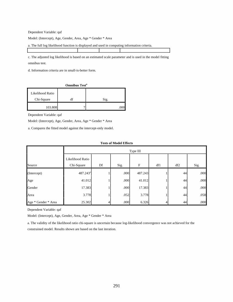
291
Dependent Variable: qaf
Model: (Intercept), Age, Gender, Area, Age * Gender * Area
a. The full log likelihood function is displayed and used in computing information criteria.
c. The adjusted log likelihood is based on an estimated scale parameter and is used in the model fitting
omnibus test.
d. Information criteria are in small-is-better form.
Omnibus Testa
Likelihood Ratio
Chi-Square df Sig.
103.808 7 .000
Dependent Variable: qaf
Model: (Intercept), Age, Gender, Area, Age * Gender * Area
a. Compares the fitted model against the intercept-only model.
Tests of Model Effects
Source
Type III
Likelihood Ratio
Chi-Square Df Sig. F df1 df2 Sig.
(Intercept) 487.243a 1 .000 487.243 1 44 .000
Age 41.012 1 .000 41.012 1 44 .000
Gender 17.383 1 .000 17.383 1 44 .000
Area 3.778 1 .052 3.778 1 44 .058
Age * Gender * Area 25.302 4 .000 6.326 4 44 .000
Dependent Variable: qaf
Model: (Intercept), Age, Gender, Area, Age * Gender * Area
a. The validity of the likelihood ratio chi-square is uncertain because log-likelihood convergence was not achieved for the
constrained model. Results shown are based on the last iteration.
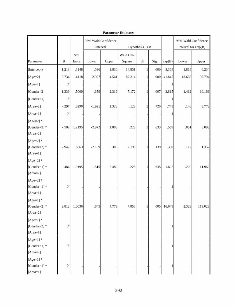
292
Parameter Estimates
Parameter B
Std.
Error
95% Wald Confidence
Interval Hypothesis Test
Exp(B)
95% Wald Confidence
Interval for Exp(B)
Lower Upper
Wald Chi-
Square df Sig. Lower Upper
(Intercept) 1.213 .3148 .596 1.830 14.851 1 .000 3.364 1.815 6.234
[Age=2] 3.734 .4118 2.927 4.541 82.214 1 .000 41.845 18.668 93.794
[Age=1] 0a . . . . . . 1 . .
[Gender=2] 1.339 .5000 .359 2.319 7.172 1 .007 3.815 1.432 10.166
[Gender=1] 0a . . . . . . 1 . .
[Area=2] -.297 .8290 -1.921 1.328 .128 1 .720 .743 .146 3.773
[Area=1] 0a . . . . . . 1 . .
[Age=2] *
[Gender=2] *
[Area=2]
-.582 1.2195 -2.972 1.808 .228 1 .633 .559 .051 6.099
[Age=2] *
[Gender=2] *
[Area=1]
-.942 .6363 -2.189 .305 2.190 1 .139 .390 .112 1.357
[Age=2] *
[Gender=1] *
[Area=2]
.484 1.0195 -1.515 2.482 .225 1 .635 1.622 .220 11.962
[Age=2] *
[Gender=1] *
[Area=1]
0a . . . . . . 1 . .
[Age=1] *
[Gender=2] *
[Area=2]
2.812 1.0036 .845 4.779 7.853 1 .005 16.649 2.329 119.023
[Age=1] *
[Gender=2] *
[Area=1]
0a . . . . . . 1 . .
[Age=1] *
[Gender=1] *
[Area=2]
0a . . . . . . 1 . .
[Age=1] *
[Gender=1] *
[Area=1]
0a . . . . . . 1 . .
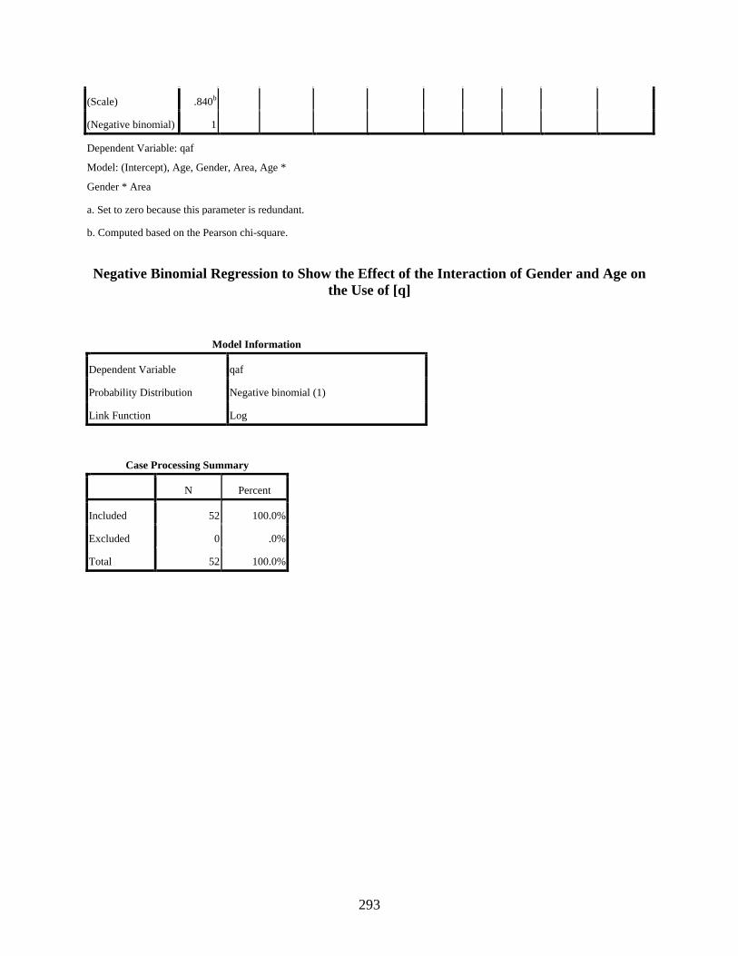
293
(Scale) .840b
(Negative binomial) 1
Dependent Variable: qaf
Model: (Intercept), Age, Gender, Area, Age *
Gender * Area
a. Set to zero because this parameter is redundant.
b. Computed based on the Pearson chi-square.
Negative Binomial Regression to Show the Effect of the Interaction of Gender and Age on
the Use of [q]
Model Information
Dependent Variable qaf
Probability Distribution Negative binomial (1)
Link Function Log
Case Processing Summary
N Percent
Included 52 100.0%
Excluded 0 .0%
Total 52 100.0%
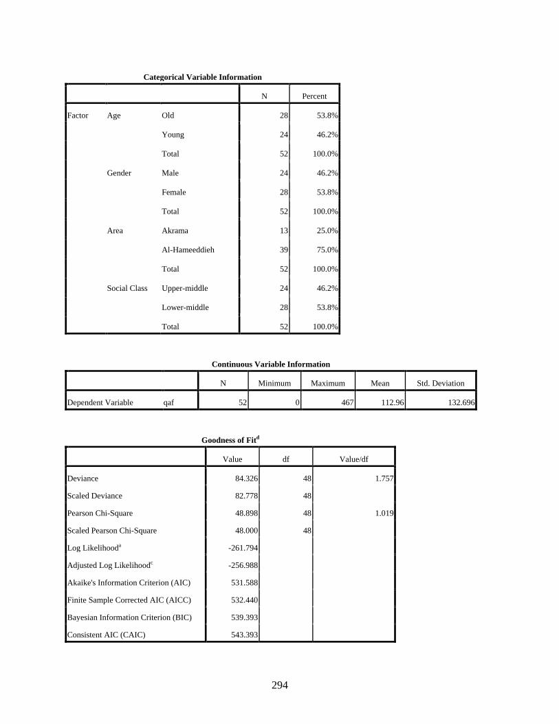
294
Categorical Variable Information
N Percent
Factor Age Old 28 53.8%
Young 24 46.2%
Total 52 100.0%
Gender Male 24 46.2%
Female 28 53.8%
Total 52 100.0%
Area Akrama 13 25.0%
Al-Hameeddieh 39 75.0%
Total 52 100.0%
Social Class Upper-middle 24 46.2%
Lower-middle 28 53.8%
Total 52 100.0%
Continuous Variable Information
N Minimum Maximum Mean Std. Deviation
Dependent Variable qaf 52 0 467 112.96 132.696
Goodness of Fitd
Value df Value/df
Deviance 84.326 48 1.757
Scaled Deviance 82.778 48
Pearson Chi-Square 48.898 48 1.019
Scaled Pearson Chi-Square 48.000 48
Log Likelihooda -261.794
Adjusted Log Likelihoodc -256.988
Akaike's Information Criterion (AIC) 531.588
Finite Sample Corrected AIC (AICC) 532.440
Bayesian Information Criterion (BIC) 539.393
Consistent AIC (CAIC) 543.393
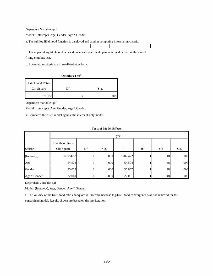
295
Dependent Variable: qaf
Model: (Intercept), Age, Gender, Age * Gender
a. The full log likelihood function is displayed and used in computing information criteria.
c. The adjusted log likelihood is based on an estimated scale parameter and is used in the model
fitting omnibus test.
d. Information criteria are in small-is-better form.
Omnibus Testa
Likelihood Ratio
Chi-Square Df Sig.
71.153 3 .000
Dependent Variable: qaf
Model: (Intercept), Age, Gender, Age * Gender
a. Compares the fitted model against the intercept-only model.
Tests of Model Effects
Source
Type III
Likelihood Ratio
Chi-Square Df Sig. F df1 df2 Sig.
(Intercept) 1702.422a 1 .000 1702.422 1 48 .000
Age 54.524 1 .000 54.524 1 48 .000
Gender 35.057 1 .000 35.057 1 48 .000
Age * Gender 22.061 1 .000 22.061 1 48 .000
Dependent Variable: qaf
Model: (Intercept), Age, Gender, Age * Gender
a. The validity of the likelihood ratio chi-square is uncertain because log-likelihood convergence was not achieved for the
constrained model. Results shown are based on the last iteration.

296
Parameter Estimates
Parameter B
Std.
Error
95% Wald Confidence
Interval Hypothesis Test
Exp(B)
95% Wald Confidence
Interval for Exp(B)
Lower Upper
Wald Chi-
Square df Sig. Lower Upper
(Intercept) 1.173 .3203 .545 1.801 13.402 1 .000 3.231 1.724 6.053
[Age=2] 3.815 .4135 3.004 4.625 85.095 1 .000 45.356 20.167 102.003
[Age=1] 0a . . . . . . 1 . .
[Gender=2] 3.199 .4432 2.330 4.068 52.108 1 .000 24.509 10.282 58.417
[Gender=1] 0a . . . . . . 1 . .
[Age=2] *
[Gender=2] -2.827 .5861 -3.976 -1.678 23.269 1 .000 .059 .019 .187
[Age=2] *
[Gender=1] 0a . . . . . . 1 . .
[Age=1] *
[Gender=2] 0a . . . . . . 1 . .
[Age=1] *
[Gender=1] 0a . . . . . . 1 . .
(Scale) 1.019b
(Negative
binomial) 1
Dependent Variable: qaf
Model: (Intercept), Age, Gender, Age * Gender
a. Set to zero because this parameter is redundant.
b. Computed based on the Pearson chi-square.

297
APPENDIX D GENERALIZED LINEAR MODELS RESULTS FOR THE DEPENDENT VARIABLE []
Negative Binomial Regression to Show the Effect of Gender, Age, Residential Area, and Social Class on the Use of []
Model Information
Dependent Variable hamza
Probability Distribution Negative binomial (1)
Link Function Log
Case Processing Summary
N Percent
Included 52 100.0%
Excluded 0 .0%
Total 52 100.0%
Categorical Variable Information
N Percent
Factor Age Old 28 53.8%
Young 24 46.2%
Total 52 100.0%
Gender Male 24 46.2%
Female 28 53.8%
Total 52 100.0%
Area Akrama 13 25.0%
Al-Hameeddieh 39 75.0%
Total 52 100.0%
Social Class Upper-middle 24 46.2%
Lower-middle 28 53.8%
Total 52 100.0%
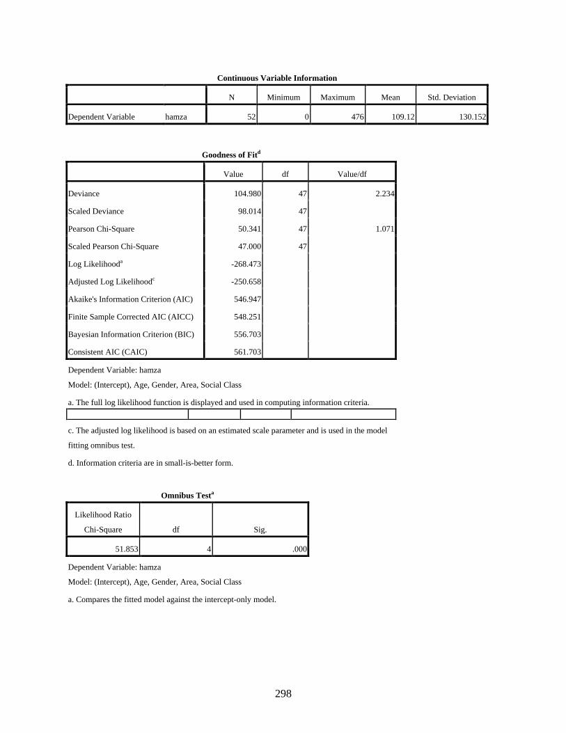
298
Continuous Variable Information
N Minimum Maximum Mean Std. Deviation
Dependent Variable hamza 52 0 476 109.12 130.152
Goodness of Fitd
Value df Value/df
Deviance 104.980 47 2.234
Scaled Deviance 98.014 47
Pearson Chi-Square 50.341 47 1.071
Scaled Pearson Chi-Square 47.000 47
Log Likelihooda -268.473
Adjusted Log Likelihoodc -250.658
Akaike's Information Criterion (AIC) 546.947
Finite Sample Corrected AIC (AICC) 548.251
Bayesian Information Criterion (BIC) 556.703
Consistent AIC (CAIC) 561.703
Dependent Variable: hamza
Model: (Intercept), Age, Gender, Area, Social Class
a. The full log likelihood function is displayed and used in computing information criteria.
c. The adjusted log likelihood is based on an estimated scale parameter and is used in the model
fitting omnibus test.
d. Information criteria are in small-is-better form.
Omnibus Testa
Likelihood Ratio
Chi-Square df Sig.
51.853 4 .000
Dependent Variable: hamza
Model: (Intercept), Age, Gender, Area, Social Class
a. Compares the fitted model against the intercept-only model.
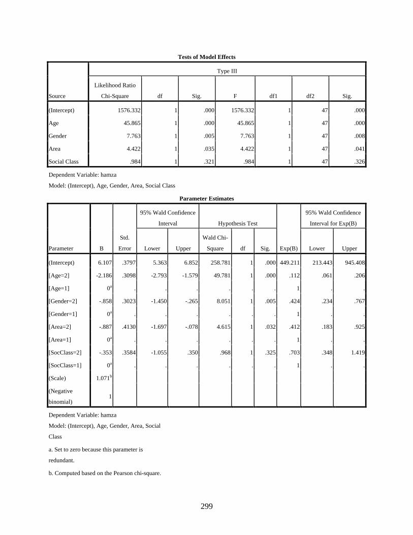
299
Tests of Model Effects
Source
Type III
Likelihood Ratio
Chi-Square df Sig. F df1 df2 Sig.
(Intercept) 1576.332 1 .000 1576.332 1 47 .000
Age 45.865 1 .000 45.865 1 47 .000
Gender 7.763 1 .005 7.763 1 47 .008
Area 4.422 1 .035 4.422 1 47 .041
Social Class .984 1 .321 .984 1 47 .326
Dependent Variable: hamza
Model: (Intercept), Age, Gender, Area, Social Class
Parameter Estimates
Parameter B
Std.
Error
95% Wald Confidence
Interval Hypothesis Test
Exp(B)
95% Wald Confidence
Interval for Exp(B)
Lower Upper
Wald Chi-
Square df Sig. Lower Upper
(Intercept) 6.107 .3797 5.363 6.852 258.781 1 .000 449.211 213.443 945.408
[Age=2] -2.186 .3098 -2.793 -1.579 49.781 1 .000 .112 .061 .206
[Age=1] 0a . . . . . . 1 . .
[Gender=2] -.858 .3023 -1.450 -.265 8.051 1 .005 .424 .234 .767
[Gender=1] 0a . . . . . . 1 . .
[Area=2] -.887 .4130 -1.697 -.078 4.615 1 .032 .412 .183 .925
[Area=1] 0a . . . . . . 1 . .
[SocClass=2] -.353 .3584 -1.055 .350 .968 1 .325 .703 .348 1.419
[SocClass=1] 0a . . . . . . 1 . .
(Scale) 1.071b
(Negative
binomial) 1
Dependent Variable: hamza
Model: (Intercept), Age, Gender, Area, Social
Class
a. Set to zero because this parameter is
redundant.
b. Computed based on the Pearson chi-square.
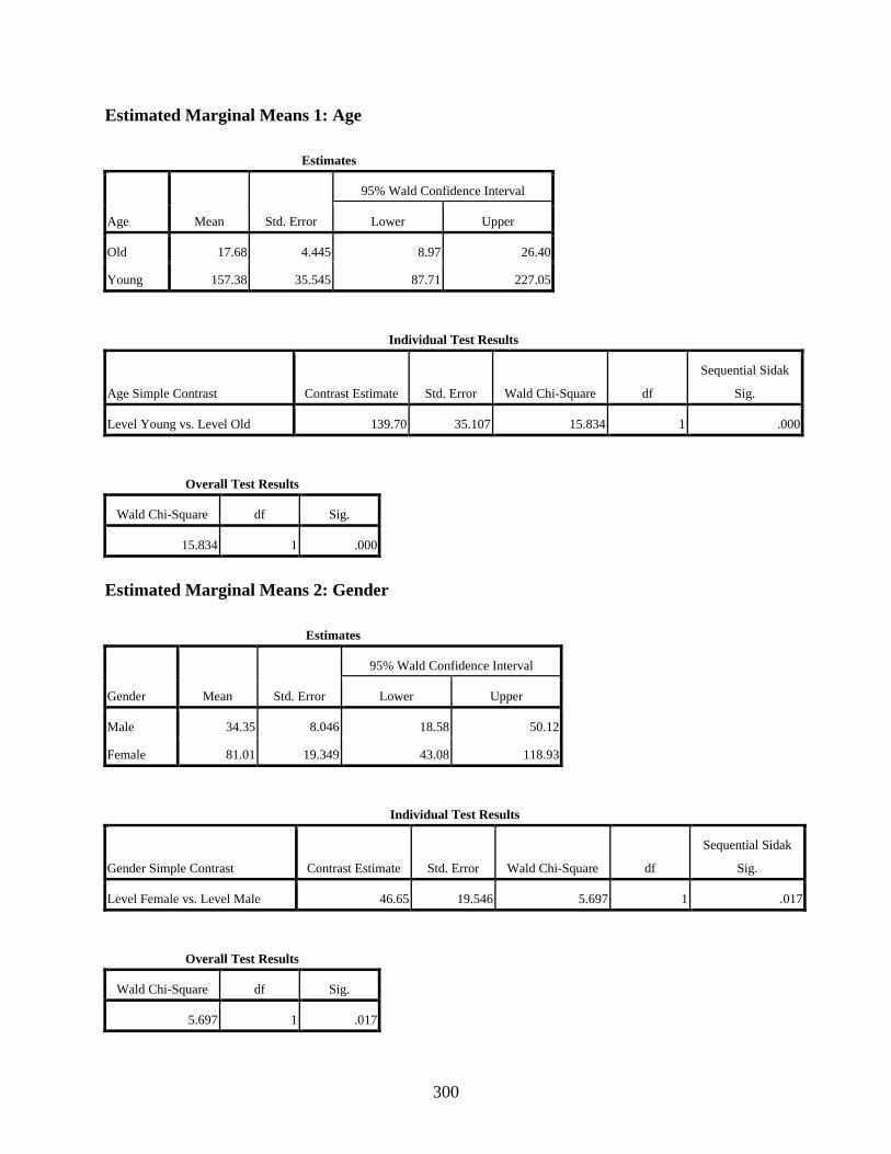
300
Estimated Marginal Means 1: Age
Estimates
Age Mean Std. Error
95% Wald Confidence Interval
Lower Upper
Old 17.68 4.445 8.97 26.40
Young 157.38 35.545 87.71 227.05
Individual Test Results
Age Simple Contrast Contrast Estimate Std. Error Wald Chi-Square df
Sequential Sidak
Sig.
Level Young vs. Level Old 139.70 35.107 15.834 1 .000
Overall Test Results
Wald Chi-Square df Sig.
15.834 1 .000
Estimated Marginal Means 2: Gender
Estimates
Gender Mean Std. Error
95% Wald Confidence Interval
Lower Upper
Male 34.35 8.046 18.58 50.12
Female 81.01 19.349 43.08 118.93
Individual Test Results
Gender Simple Contrast Contrast Estimate Std. Error Wald Chi-Square df
Sequential Sidak
Sig.
Level Female vs. Level Male 46.65 19.546 5.697 1 .017
Overall Test Results
Wald Chi-Square df Sig.
5.697 1 .017
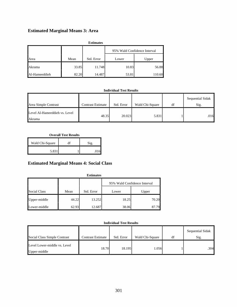
301
Estimated Marginal Means 3: Area
Estimates
Area Mean Std. Error
95% Wald Confidence Interval
Lower Upper
Akrama 33.85 11.748 10.83 56.88
Al-Hameeddieh 82.20 14.487 53.81 110.60
Individual Test Results
Area Simple Contrast Contrast Estimate Std. Error Wald Chi-Square df
Sequential Sidak
Sig.
Level Al-Hameeddieh vs. Level
Akrama 48.35 20.023 5.831 1 .016
Overall Test Results
Wald Chi-Square df Sig.
5.831 1 .016
Estimated Marginal Means 4: Social Class
Estimates
Social Class Mean Std. Error
95% Wald Confidence Interval
Lower Upper
Upper-middle 44.22 13.252 18.25 70.20
Lower-middle 62.93 12.687 38.06 87.79
Individual Test Results
Social Class Simple Contrast Contrast Estimate Std. Error Wald Chi-Square df
Sequential Sidak
Sig.
Level Lower-middle vs. Level
Upper-middle 18.70 18.195 1.056 1 .304
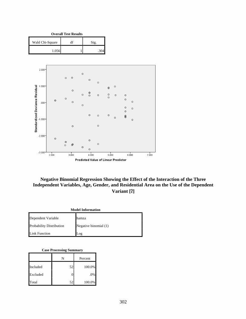
302
Overall Test Results
Wald Chi-Square df Sig.
1.056 1 .304
Negative Binomial Regression Showing the Effect of the Interaction of the Three Independent Variables, Age, Gender, and Residential Area on the Use of the Dependent
Variant []
Model Information
Dependent Variable hamza
Probability Distribution Negative binomial (1)
Link Function Log
Case Processing Summary
N Percent
Included 52 100.0%
Excluded 0 .0%
Total 52 100.0%

303
Categorical Variable Information
N Percent
Factor Age Old 28 53.8%
Young 24 46.2%
Total 52 100.0%
Gender Male 24 46.2%
Female 28 53.8%
Total 52 100.0%
Area Akrama 13 25.0%
Al-Hameeddieh 39 75.0%
Total 52 100.0%
Social Class Upper-middle 24 46.2%
Lower-middle 28 53.8%
Total 52 100.0%
Continuous Variable Information
N Minimum Maximum Mean Std. Deviation
Dependent Variable hamza 52 0 476 109.12 130.152
Goodness of Fitd
Value df Value/df
Deviance 101.808 44 2.314
Scaled Deviance 98.283 44
Pearson Chi-Square 45.578 44 1.036
Scaled Pearson Chi-Square 44.000 44
Log Likelihooda -266.887
Adjusted Log Likelihoodc -257.647
Akaike's Information Criterion (AIC) 549.775
Finite Sample Corrected AIC (AICC) 553.124
Bayesian Information Criterion (BIC) 565.385
Consistent AIC (CAIC) 573.385
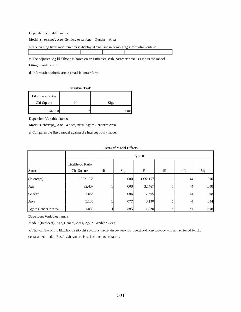
304
Dependent Variable: hamza
Model: (Intercept), Age, Gender, Area, Age * Gender * Area
a. The full log likelihood function is displayed and used in computing information criteria.
c. The adjusted log likelihood is based on an estimated scale parameter and is used in the model
fitting omnibus test.
d. Information criteria are in small-is-better form.
Omnibus Testa
Likelihood Ratio
Chi-Square df Sig.
56.678 7 .000
Dependent Variable: hamza
Model: (Intercept), Age, Gender, Area, Age * Gender * Area
a. Compares the fitted model against the intercept-only model.
Tests of Model Effects
Source
Type III
Likelihood Ratio
Chi-Square df Sig. F df1 df2 Sig.
(Intercept) 1332.157a 1 .000 1332.157 1 44 .000
Age 32.467 1 .000 32.467 1 44 .000
Gender 7.665 1 .006 7.665 1 44 .008
Area 3.130 1 .077 3.130 1 44 .084
Age * Gender * Area 4.080 4 .395 1.020 4 44 .408
Dependent Variable: hamza
Model: (Intercept), Age, Gender, Area, Age * Gender * Area
a. The validity of the likelihood ratio chi-square is uncertain because log-likelihood convergence was not achieved for the
constrained model. Results shown are based on the last iteration.
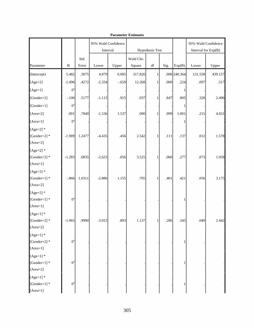
305
Parameter Estimates
Parameter B
Std.
Error
95% Wald Confidence
Interval Hypothesis Test
Exp(B)
95% Wald Confidence
Interval for Exp(B)
Lower Upper
Wald Chi-
Square df Sig. Lower Upper
(Intercept) 5.482 .3075 4.879 6.085 317.826 1 .000 240.364 131.558 439.157
[Age=2] -1.496 .4272 -2.334 -.659 12.268 1 .000 .224 .097 .517
[Age=1] 0a . . . . . . 1 . .
[Gender=2] -.100 .5177 -1.115 .915 .037 1 .847 .905 .328 2.496
[Gender=1] 0a . . . . . . 1 . .
[Area=2] .001 .7840 -1.536 1.537 .000 1 .999 1.001 .215 4.651
[Area=1] 0a . . . . . . 1 . .
[Age=2] *
[Gender=2] *
[Area=2]
-1.989 1.2477 -4.435 .456 2.542 1 .111 .137 .012 1.578
[Age=2] *
[Gender=2] *
[Area=1]
-1.283 .6835 -2.623 .056 3.525 1 .060 .277 .073 1.058
[Age=2] *
[Gender=1] *
[Area=2]
-.866 1.0311 -2.886 1.155 .705 1 .401 .421 .056 3.175
[Age=2] *
[Gender=1] *
[Area=1]
0a . . . . . . 1 . .
[Age=1] *
[Gender=2] *
[Area=2]
-1.065 .9990 -3.023 .893 1.137 1 .286 .345 .049 2.442
[Age=1] *
[Gender=2] *
[Area=1]
0a . . . . . . 1 . .
[Age=1] *
[Gender=1] *
[Area=2]
0a . . . . . . 1 . .
[Age=1] *
[Gender=1] *
[Area=1]
0a . . . . . . 1 . .
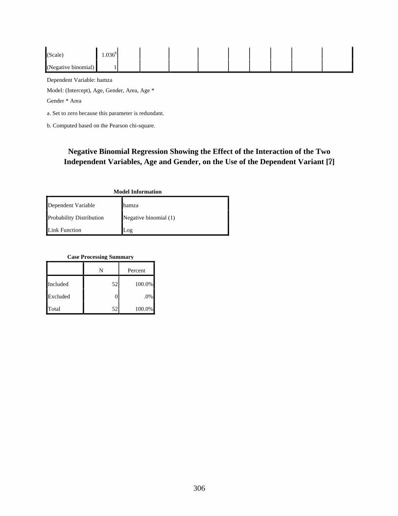
306
(Scale) 1.036b
(Negative binomial) 1
Dependent Variable: hamza
Model: (Intercept), Age, Gender, Area, Age *
Gender * Area
a. Set to zero because this parameter is redundant.
b. Computed based on the Pearson chi-square.
Negative Binomial Regression Showing the Effect of the Interaction of the Two Independent Variables, Age and Gender, on the Use of the Dependent Variant []
Model Information
Dependent Variable hamza
Probability Distribution Negative binomial (1)
Link Function Log
Case Processing Summary
N Percent
Included 52 100.0%
Excluded 0 .0%
Total 52 100.0%
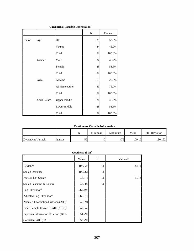
307
Categorical Variable Information
N Percent
Factor Age Old 28 53.8%
Young 24 46.2%
Total 52 100.0%
Gender Male 24 46.2%
Female 28 53.8%
Total 52 100.0%
Area Akrama 13 25.0%
Al-Hameeddieh 39 75.0%
Total 52 100.0%
Social Class Upper-middle 24 46.2%
Lower-middle 28 53.8%
Total 52 100.0%
Continuous Variable Information
N Minimum Maximum Mean Std. Deviation
Dependent Variable hamza 52 0 476 109.12 130.152
Goodness of Fitd
Value df Value/df
Deviance 107.027 48 2.230
Scaled Deviance 105.764 48
Pearson Chi-Square 48.573 48 1.012
Scaled Pearson Chi-Square 48.000 48
Log Likelihooda -269.497
Adjusted Log Likelihoodc -266.317
Akaike's Information Criterion (AIC) 546.994
Finite Sample Corrected AIC (AICC) 547.845
Bayesian Information Criterion (BIC) 554.799
Consistent AIC (CAIC) 558.799

308
Dependent Variable: hamza
Model: (Intercept), Age, Gender, Age * Gender
a. The full log likelihood function is displayed and used in computing information criteria.
c. The adjusted log likelihood is based on an estimated scale parameter and is used in the model fitting
omnibus test.
d. Information criteria are in small-is-better form.
Omnibus Testa
Likelihood Ratio
Chi-Square df Sig.
52.860 3 .000
Dependent Variable: hamza
Model: (Intercept), Age, Gender, Age * Gender
a. Compares the fitted model against the intercept-only model.
Tests of Model Effects
Source
Type III
Likelihood Ratio
Chi-Square df Sig. F df1 df2 Sig.
(Intercept) 2618.410 1 .000 2618.410 1 48 .000
Age 48.470 1 .000 48.470 1 48 .000
Gender 9.883 1 .002 9.883 1 48 .003
Age * Gender 2.658 1 .103 2.658 1 48 .110
Dependent Variable: hamza
Model: (Intercept), Age, Gender, Age * Gender
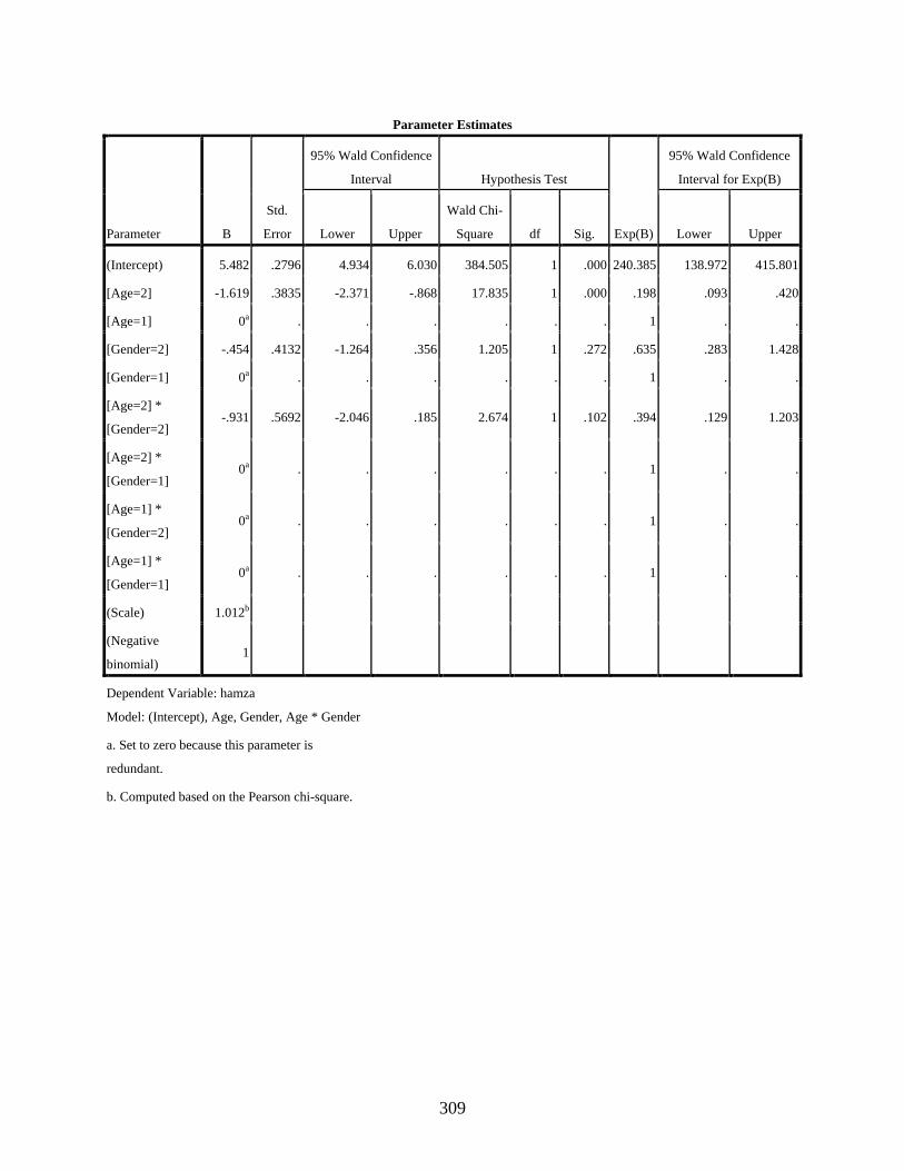
309
Parameter Estimates
Parameter B
Std.
Error
95% Wald Confidence
Interval Hypothesis Test
Exp(B)
95% Wald Confidence
Interval for Exp(B)
Lower Upper
Wald Chi-
Square df Sig. Lower Upper
(Intercept) 5.482 .2796 4.934 6.030 384.505 1 .000 240.385 138.972 415.801
[Age=2] -1.619 .3835 -2.371 -.868 17.835 1 .000 .198 .093 .420
[Age=1] 0a . . . . . . 1 . .
[Gender=2] -.454 .4132 -1.264 .356 1.205 1 .272 .635 .283 1.428
[Gender=1] 0a . . . . . . 1 . .
[Age=2] *
[Gender=2] -.931 .5692 -2.046 .185 2.674 1 .102 .394 .129 1.203
[Age=2] *
[Gender=1] 0a . . . . . . 1 . .
[Age=1] *
[Gender=2] 0a . . . . . . 1 . .
[Age=1] *
[Gender=1] 0a . . . . . . 1 . .
(Scale) 1.012b
(Negative
binomial) 1
Dependent Variable: hamza
Model: (Intercept), Age, Gender, Age * Gender
a. Set to zero because this parameter is
redundant.
b. Computed based on the Pearson chi-square.
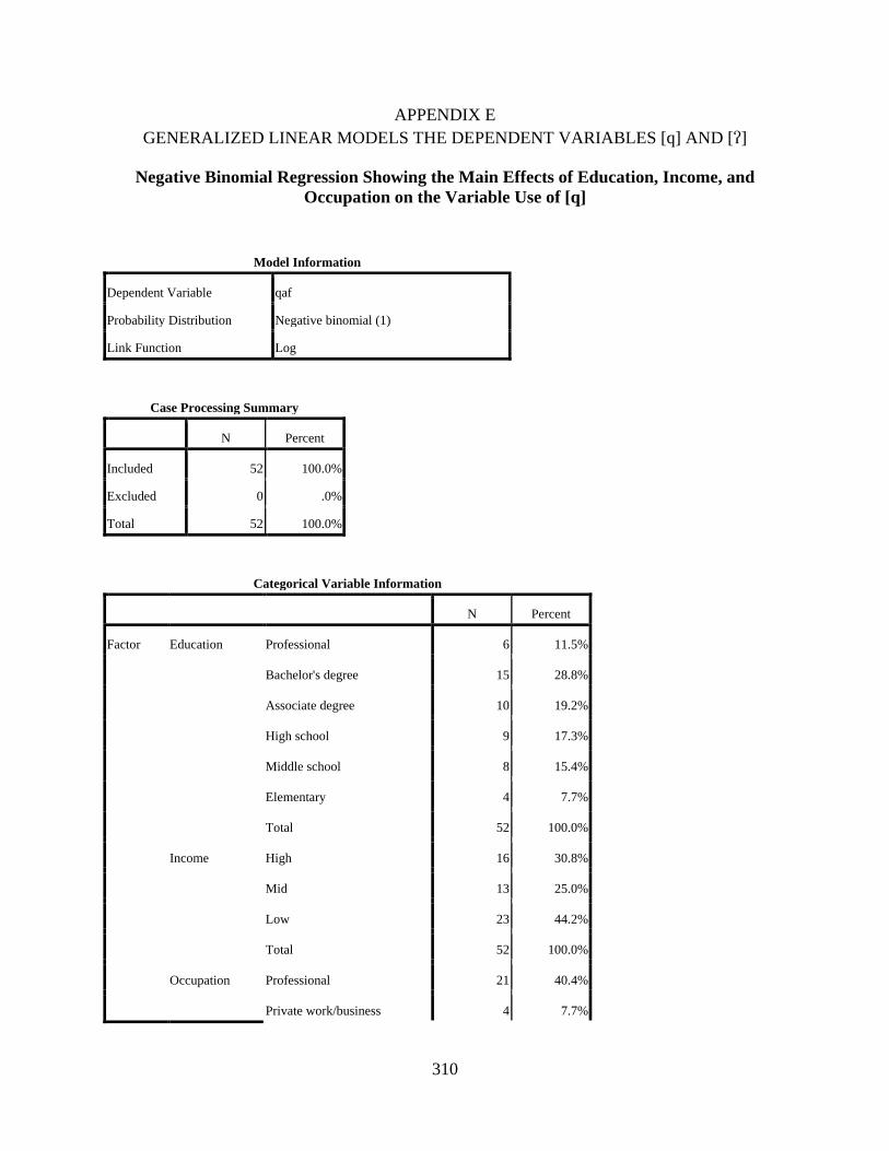
310
APPENDIX E GENERALIZED LINEAR MODELS THE DEPENDENT VARIABLES [q] AND []
Negative Binomial Regression Showing the Main Effects of Education, Income, and Occupation on the Variable Use of [q]
Model Information
Dependent Variable qaf
Probability Distribution Negative binomial (1)
Link Function Log
Case Processing Summary
N Percent
Included 52 100.0%
Excluded 0 .0%
Total 52 100.0%
Categorical Variable Information
N Percent
Factor Education Professional 6 11.5%
Bachelor's degree 15 28.8%
Associate degree 10 19.2%
High school 9 17.3%
Middle school 8 15.4%
Elementary 4 7.7%
Total 52 100.0%
Income High 16 30.8%
Mid 13 25.0%
Low 23 44.2%
Total 52 100.0%
Occupation Professional 21 40.4%
Private work/business 4 7.7%
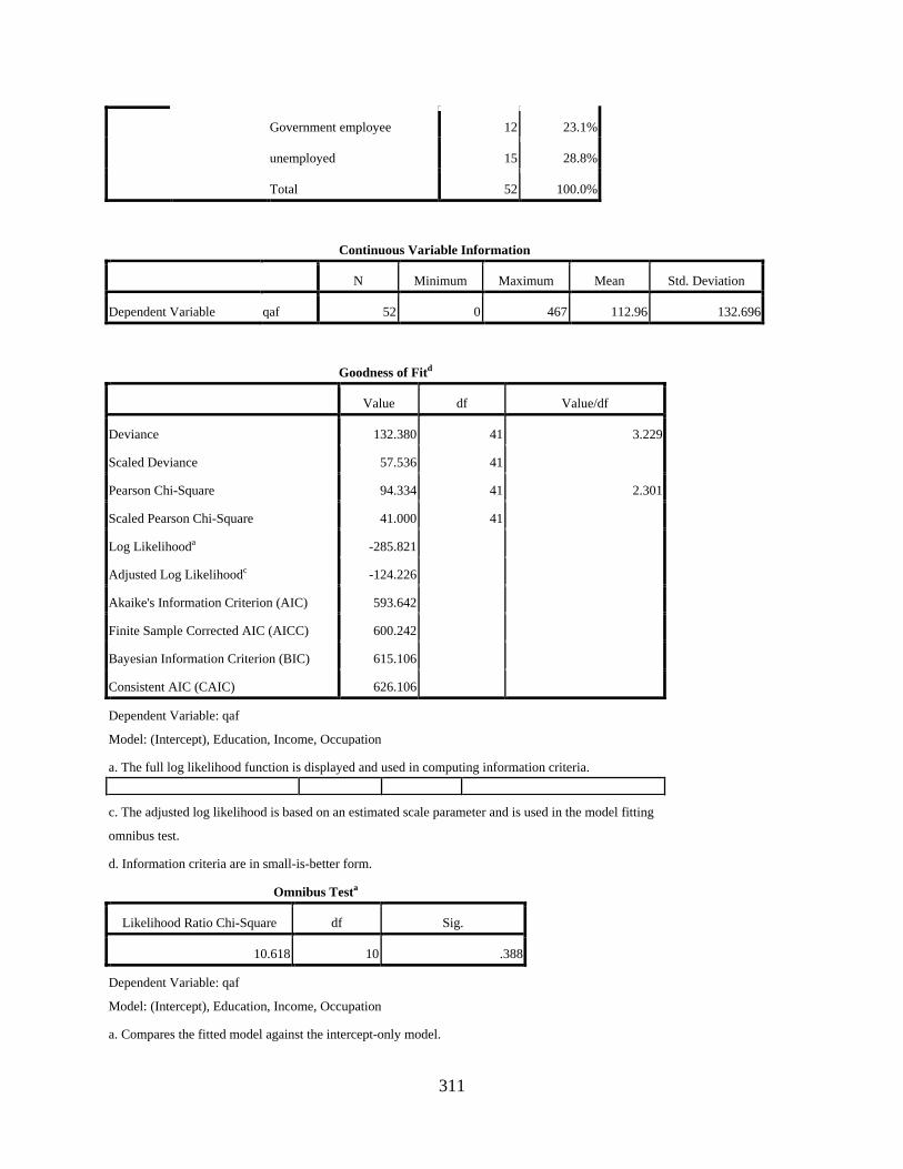
311
Government employee 12 23.1%
unemployed 15 28.8%
Total 52 100.0%
Continuous Variable Information
N Minimum Maximum Mean Std. Deviation
Dependent Variable qaf 52 0 467 112.96 132.696
Goodness of Fitd
Value df Value/df
Deviance 132.380 41 3.229
Scaled Deviance 57.536 41
Pearson Chi-Square 94.334 41 2.301
Scaled Pearson Chi-Square 41.000 41
Log Likelihooda -285.821
Adjusted Log Likelihoodc -124.226
Akaike's Information Criterion (AIC) 593.642
Finite Sample Corrected AIC (AICC) 600.242
Bayesian Information Criterion (BIC) 615.106
Consistent AIC (CAIC) 626.106
Dependent Variable: qaf
Model: (Intercept), Education, Income, Occupation
a. The full log likelihood function is displayed and used in computing information criteria.
c. The adjusted log likelihood is based on an estimated scale parameter and is used in the model fitting
omnibus test.
d. Information criteria are in small-is-better form.
Omnibus Testa
Likelihood Ratio Chi-Square df Sig.
10.618 10 .388
Dependent Variable: qaf
Model: (Intercept), Education, Income, Occupation
a. Compares the fitted model against the intercept-only model.
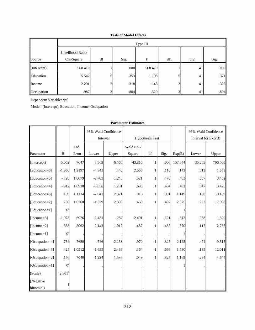
312
Tests of Model Effects
Source
Type III
Likelihood Ratio
Chi-Square df Sig. F df1 df2 Sig.
(Intercept) 568.410 1 .000 568.410 1 41 .000
Education 5.542 5 .353 1.108 5 41 .371
Income 2.291 2 .318 1.145 2 41 .328
Occupation .987 3 .804 .329 3 41 .804
Dependent Variable: qaf
Model: (Intercept), Education, Income, Occupation
Parameter Estimates
Parameter B
Std.
Error
95% Wald Confidence
Interval Hypothesis Test
Exp(B)
95% Wald Confidence
Interval for Exp(B)
Lower Upper
Wald Chi-
Square df Sig. Lower Upper
(Intercept) 5.062 .7647 3.563 6.560 43.816 1 .000 157.844 35.265 706.500
[Education=6] -1.950 1.2197 -4.341 .440 2.556 1 .110 .142 .013 1.553
[Education=5] -.728 1.0079 -2.703 1.248 .521 1 .470 .483 .067 3.482
[Education=4] -.912 1.0938 -3.056 1.231 .696 1 .404 .402 .047 3.426
[Education=3] .139 1.1134 -2.043 2.321 .016 1 .901 1.149 .130 10.189
[Education=2] .730 1.0760 -1.379 2.839 .460 1 .497 2.075 .252 17.098
[Education=1] 0a . . . . . . 1 . .
[Income=3] -1.073 .6926 -2.431 .284 2.401 1 .121 .342 .088 1.329
[Income=2] -.563 .8062 -2.143 1.017 .487 1 .485 .570 .117 2.766
[Income=1] 0a . . . . . . 1 . .
[Occupation=4] .754 .7650 -.746 2.253 .970 1 .325 2.125 .474 9.515
[Occupation=3] .425 1.0512 -1.635 2.486 .164 1 .686 1.530 .195 12.011
[Occupation=2] .156 .7040 -1.224 1.536 .049 1 .825 1.169 .294 4.644
[Occupation=1] 0a . . . . . . 1 . .
(Scale) 2.301b
(Negative
binomial) 1
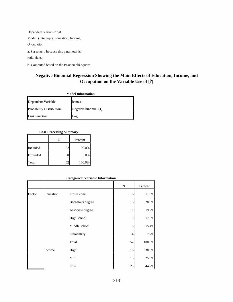
313
Dependent Variable: qaf
Model: (Intercept), Education, Income,
Occupation
a. Set to zero because this parameter is
redundant.
b. Computed based on the Pearson chi-square.
Negative Binomial Regression Showing the Main Effects of Education, Income, and Occupation on the Variable Use of []
Model Information
Dependent Variable hamza
Probability Distribution Negative binomial (1)
Link Function Log
Case Processing Summary
N Percent
Included 52 100.0%
Excluded 0 .0%
Total 52 100.0%
Categorical Variable Information
N Percent
Factor Education Professional 6 11.5%
Bachelor's degree 15 28.8%
Associate degree 10 19.2%
High school 9 17.3%
Middle school 8 15.4%
Elementary 4 7.7%
Total 52 100.0%
Income High 16 30.8%
Mid 13 25.0%
Low 23 44.2%
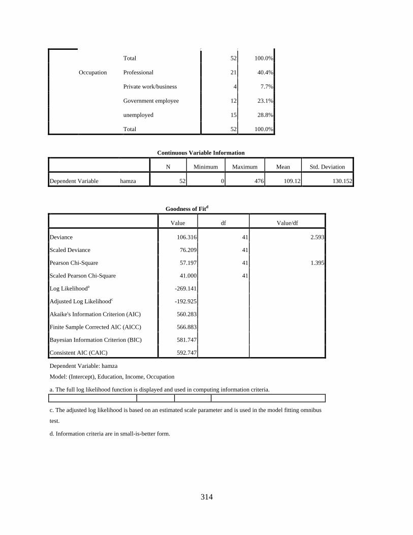
314
Total 52 100.0%
Occupation Professional 21 40.4%
Private work/business 4 7.7%
Government employee 12 23.1%
unemployed 15 28.8%
Total 52 100.0%
Continuous Variable Information
N Minimum Maximum Mean Std. Deviation
Dependent Variable hamza 52 0 476 109.12 130.152
Goodness of Fitd
Value df Value/df
Deviance 106.316 41 2.593
Scaled Deviance 76.209 41
Pearson Chi-Square 57.197 41 1.395
Scaled Pearson Chi-Square 41.000 41
Log Likelihooda -269.141
Adjusted Log Likelihoodc -192.925
Akaike's Information Criterion (AIC) 560.283
Finite Sample Corrected AIC (AICC) 566.883
Bayesian Information Criterion (BIC) 581.747
Consistent AIC (CAIC) 592.747
Dependent Variable: hamza
Model: (Intercept), Education, Income, Occupation
a. The full log likelihood function is displayed and used in computing information criteria.
c. The adjusted log likelihood is based on an estimated scale parameter and is used in the model fitting omnibus
test.
d. Information criteria are in small-is-better form.
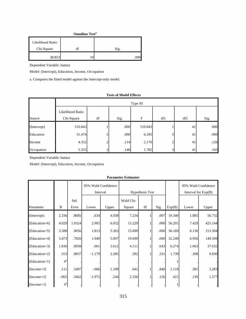
315
Omnibus Testa
Likelihood Ratio
Chi-Square df Sig.
38.853 10 .000
Dependent Variable: hamza
Model: (Intercept), Education, Income, Occupation
a. Compares the fitted model against the intercept-only model.
Tests of Model Effects
Source
Type III
Likelihood Ratio
Chi-Square df Sig. F df1 df2 Sig.
(Intercept) 510.843 1 .000 510.843 1 41 .000
Education 31.474 5 .000 6.295 5 41 .000
Income 4.352 2 .114 2.176 2 41 .126
Occupation 5.355 3 .148 1.785 3 41 .165
Dependent Variable: hamza
Model: (Intercept), Education, Income, Occupation
Parameter Estimates
Parameter B
Std.
Error
95% Wald Confidence
Interval Hypothesis Test
Exp(B)
95% Wald Confidence
Interval for Exp(B)
Lower Upper
Wald Chi-
Square df Sig. Lower Upper
(Intercept) 2.336 .8685 .634 4.038 7.234 1 .007 10.340 1.885 56.732
[Education=6] 4.029 1.0324 2.005 6.052 15.229 1 .000 56.201 7.429 425.144
[Education=5] 3.588 .9056 1.813 5.363 15.699 1 .000 36.169 6.130 213.394
[Education=4] 3.473 .7826 1.940 5.007 19.699 1 .000 32.249 6.956 149.509
[Education=3] 1.836 .9058 .061 3.612 4.111 1 .043 6.274 1.063 37.032
[Education=2] .553 .8837 -1.179 2.285 .392 1 .531 1.739 .308 9.830
[Education=1] 0a . . . . . . 1 . .
[Income=3] .111 .5497 -.966 1.189 .041 1 .840 1.118 .381 3.283
[Income=2] -.865 .5662 -1.975 .244 2.336 1 .126 .421 .139 1.277
[Income=1] 0a . . . . . . 1 . .

316
[Occupation=4] -1.093 .5929 -2.255 .070 3.396 1 .065 .335 .105 1.072
[Occupation=3] .389 .7414 -1.064 1.842 .276 1 .600 1.476 .345 6.311
[Occupation=2] -.667 .6469 -1.935 .601 1.064 1 .302 .513 .144 1.824
[Occupation=1] 0a . . . . . . 1 . .
(Scale) 1.395b
(Negative
binomial) 1
Dependent Variable: hamza
Model: (Intercept), Education, Income,
Occupation
a. Set to zero because this parameter is
redundant.
b. Computed based on the Pearson chi-square.

317
APPENDIX F INTERNTIONAL PHONETIC ALPHABET (IPA) SYMBOLS FOR STANDARD ARABIC,
HIMSI COLLOQUIAL ARABIC, AND RURAL COLLOQUIAL ARABIC
Standard Arabic Phonemic System in IPA20
Bilabial Labio- dental
(Inter) dental
Alveolar Alveo- palatal
Palatal Velar Uvular Pharyngeal glottal
Stop b t d t d
k q
Nasal m n Affricate
d
Fricative f θ ð
s z s
ʃ h
Liquid l r
Glide w j
Himsi Colloquial Arabic Phonemic System in IPA
Bilabial Labio- dental
Alveolar Alveo- palatal
Palatal Velar Uvular Pharyngeal glottal
Stop b t d t d
k
Nasal m n Fricative f s z
s z ʃ h
Liquid l r
Glide w j
20 The sounds on the left within the same column are voiceless; the ones on the right are voiced. This applies to the other two tables.
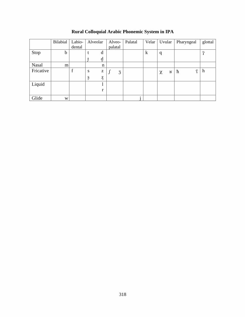
318
Rural Colloquial Arabic Phonemic System in IPA
Bilabial Labio- dental
Alveolar Alveo- palatal
Palatal Velar Uvular Pharyngeal glottal
Stop b t d t d
k q
Nasal m n Fricative f s z
s z ʃ h
Liquid l r
Glide w j
319
LIST OF REFERENCES
Abdel-Jawad, Hassan R. 1981. Phonological and social variation in Arabic in Amman. Philadelphia, PA: University of Pennsylvania dissertation.
Abd-el-Jawad, Hassan Rashid, 1986. The emergence of an urban dialect in the Jordanian urban
centers. International Journal of the Sociology of Language 61.53-63. Abu-Haidar, Farida. 1992. Shifting boundaries: The effect of MSA on dialect convergence in
Baghdad. Perspectives on Arabic linguistics IV, ed. by Ellen Broselow, Mushira Eid, and John McCarthy, 91-106. (Current Issues in Linguistic Theory 85). Amsterdam: John Benjamins.
Adam, Galit. 2002. From Variable to Optimal Grammar: Evidence from language acquisition
and language change. Tel-Aviv, Israel: Tel-Aviv University dissertation. Rutgers Optimality Archive21 ROA-567.
Agresti, Alan, and Barbara Finlay. 1997. Statistical Methods for the Social Sciences, Third
Edition. Upper Saddle River, NJ: Prentice Hall International, Inc. Al-Ani, Salman H. 1976. The development and distribution of the Arabic ‘qaf’ in Iraq. Essays on
Islamic civilization, ed. by Donald P. Little, 48-55. Leiden: E. J. Brill. [Reprinted in Readings in Arabic Linguistics (1978), ed. by Salman H. Al-Ani. Bloomington, Indiana: Indiana University Linguistics Club, 1978].
Al-Khatib, Samer. 2008. On the directionality of emphasis spread. Paper presented at the annual meeting of the Linguistics Society of America, Chicago.
Al-Wer, Enam. 1999. Why do different variables behave differently? Data from Arabic.
Language and Society in the Middle East and North Africa, ed. by Yasir Suleiman, 38-57. London: Curzon.
Al-Wer, Enam. 2002. Education as a speaker variable. Language Contact and Language Conflict
in Arabic, ed. by Aleya Rouchdy, 41-53. London: Curzon. Anttila, Arto. 1997a. Deriving variation from grammar. Variation, change and phonological
theory, ed. by Frans Hinskens, Roeland van Hout, and W. Leo Wetzels, 35-68. Amsterdam: John Benjamins.
Anttila, Arto. 1997b. Variation in Finnish phonology and morphology. Stanford, CA: Stanford University dissertation.
21 Rutgers Optimality Archive can be accessed at this website http://roa.rutgers.edu/index.php3.
320
Anttila, Arto. 2002. Variation and phonological theory. The Handbook of Language Variation and Change, ed. by Jack K. Chambers, Peter Trudgill, and Natalie Schilling-Estes, 206- 243. Oxford: Blackwell.
Anttila, Arto, and Young-mee Yu Cho. 1998. Variation and change in optimality theory. Lingua 104.31-56.
Arad, Maya. 2003. Locality constraints on the interpretation of roots: the case of Hebrew denominal verbs. Natural Language and Linguistic Theory 21.737–778.
Archangeli, Diana. 1984. Underspecification in Yawelmani Phonology and Morphology, Cambridge, MA: MIT doctoral dissertation.
Archangeli, Diana. 1988. Aspects of underspecification theory. Phonology 5.183-208. Aske, Jon. 1990. Disembodied rules vs. patterns in the lexicon: Testing the psychological reality
of Spanish stress rules. BLS 7.30–45.
Ayres-Bennett, Wendy. 2004. Sociolinguistic Variation in Seventeenth-Century France: Methodology and Case Studies. Cambridge and New York: Cambridge University Press.
Bayley, Robert. 1994. Consonant cluster reduction in Tejano English. Language Variation and Change 6.303-326.
Bell, Alan. 1984. Language style as audience design. Language in Society 13 (2).145-204. Bell, Alan. 1991. The Language of News Media. Oxford: Blackwell. Beret, Iris; Vered Vaknin; and Gary F. Marcus. 2007. Roots, stems, and the universality of
lexical representations: Evidence form Hebrew. Cognition 104 (2).254-286. Bermúdez-Otero, Ricardo, and Richard M. Hogg. 2003. The actuation problem in Optimality
Theory: phonologization, rule inversion, and rule loss. In Holt, 91-119.
Birkeland, Harris. 1952. Growth and structure of Egyptian Arabic dialect. Oslo: Avhandlinger utg. Av det Norske Videnskape-Acad.
Bod, Rens; Jennifer Hay; and Stefanie Jannedy (eds.). 2003. Probabilistic Linguistics, 289-341. Cambridge, MA: The MIT Press.
Boersma, Paul, and David Weenink. 2007. Praat: a system for doing phonetics by computer
(Version 4.6.03) [Computer program]. Retrieved May 24, 2007, from http://www.praat.org/
Boersma, Paul. 1997a. How we learn variation, optionality, and probability. The Institute of Phonetic Sciences of the University of Amsterdam 21.43–58.
321
Boersma, Paul. 1997b. Sound change in functional phonology. Rutgers Optimality Archive ROA-237, ms.
Boersma, Paul. 1998. Functional Phonology: Formalizing the Interaction between Articulatory and Perceptual Drives. Amsterdam: University of Amsterdam dissertation.
Boersma, Paul. 2000. Learning a grammar in Functional Phonology. In Dekkers, van
der Leeuw, and van de Weijer, 465-523.
Boersma, Paul. 2001. Praat: a system for doing phonetics by computer. Glot international 5:9/10.341-345.
Boersma, Paul, and Bruce Hayes. 2001. Empirical Tests of the Gradual Learning Algorithm. Linguistic Inquiry 32 (1).45–86.
Bybee, Joan L. 1985. Morphology as lexical organization: evidence from lexical diffusion. Theoretical Morphology, ed. by Michael Hammond, and Michael Noonan, 119-41. San Diego, CA: Academic Press.
Bybee, Joan L. 2000. The phonology of the lexicon: evidence from lexical diffusion.
Usage-based models of language, ed. by Michael Barlow and Suzanne Kemmer, 65-85. Stanford, CA: CSLI.
Bybee, Joan L. 2001. Phonology and Language Use. (Cambridge Studies in Linguistics 94). Cambridge: Cambridge University Press.
Bybee, Joan L. 2002. Word frequency and context of use in the lexical diffusion of phonetically
conditioned sound change. Language Variation and Change 14.261-290. Bybee, Joan L. 2003. Mechanisms of change in grammaticization: the role of frequency.
The Handbook of Historical Linguistics, ed. by Brian D. Joseph and Richard D. Janda, 602-623. Oxford: Blackwell.
Bybee, Joan L., and James L. McClelland. 2005. Alternatives to the combinatorial paradigm of
linguistic theory based on domain general principles of human cognition. The Linguistic Review 22.381-410.
Cameron, Deborah, 1998. Performing gender identity: Young men’s talk and the construction of
heterosexual masculinity. Language and Gender. A Reader, ed. by Jennifer Coates, 270-284. Oxford: Blackwell.
Chambers, Jack K.; Peter Trudgill; and Natalie Schilling-Estes (eds.). 2002. The Handbook of
Language Variation and Change. Malden, MA: Blackwell.
Chomsky, Noam. 1980. Rules and Representations. Behavioral and Brain Sciences 3. 1-61.
322
Churchyard, Henry. 1993. Early Arabic siin and siin in light of the proto-Semitic fricative-lateral hypothesis. Perspectives on Arabic linguistics V: Papers from the Fifth Annual Symposium on Arabic Linguistics, ed. by Mushira Eid and Clive Holes, 313-342. Amsterdam: John Benjamins.
Clements, George N. 1985. The geometry of phonological features. In Phonology Yearbook 2,
225-252. Cambridge: Cambridge University Press. Clements, George N. 1990. The role of sonority cycle in core syllabification. Papers in
Laboratory Phonology I: Between the Grammar and Physics of Speech, ed. by John Kingston and Mary F. Beckman, 283-333. Cambridge: Cambridge University Press.
Coates, Jennifer. 1996. Women, Men and Language. London: Longman Group Limited. Coetzee, Andries W. 2008. Phonological Variation and Lexical Frequency. ‘Short’ version to
appear in the Proceedings of the 38th Annual Meeting of the North East Linguistics Society (NELS 38). Rutgers Optimality Archive ROA-952, ms.
Coupland, Nikolas. 1980. Style-shifting in a Cardiff work-setting. Language in Society 9.1-12. Coupland, Nikolas. 1985. Hark, hark the lark: Social motivations for phonological style-
shifting. Language and Communication 5 (3).195-72. Coupland, Nikolas. 2001. Dialect stylization in radio talk. Language in society 30 (3).345-75. Cutillas-Espinosa, Juan A. 2004. Meaningful variability: A sociolinguistically-grounded
approach to variation in Optimality theory. International Journal of English Studies 4 (2).165-184.
Cutillas-Espinosa, Juan Antonio, and Juan Manuel Hernández-Campoy. 2004. Audience and
speaker design in radio broadcasting: Attitudes to language as a starting script. Universidad de Murcia, ms.
Daher, Jamil. 1998a. Linguistic variation in Damascus Arabic: A quantitative analysis of men's
and women's speech. New York, NY: New York University dissertation.
Daher, Jamil. 1998b. Gender in linguistic variation: The variable (q) in Damascus Arabic. Perspectives on Arabic linguistics XI: Papers from the Eleventh Annual Symposium on Arabic Linguistics, ed. by Elabbas Benmamoun, Mushira Eid, and John McCarthy, 183-206. Amsterdam: John Benjamins.
Daher, Jamil. 1999. ((theta)) and ((eth)) as Ternary and Binary Variables in Damascene Arabic.
Perspectives on Arabic linguistics XII: Papers from the Twelfth Annual Symposium on Arabic Linguistics, ed. by Elabbas Benmamoun, 163-182. Amsterdam: John Benjamins.
323
Davis, Stuart. 1993. Arabic pharyngealization and phonological features. Perspectives on Arabic linguistics V, ed. by Mushira Eid and Clive Holes, 49-162. Amsterdam: John Benjamins.
Davis, Stuart. 1995. Emphasis spread in Arabic and grounded phonology. Linguistic Inquiry 26 (3).465-498.
Davis, Stuart, and Zawaydeh, Bushra A. 2001. Arabic hypocoristics and the status of the
consonantal root. Linguistic Inquiry 32.512–520. Dekkers, Joost; Frank van der Leeuw; and Jeroen van de Weijer (eds.) 2000. Optimality Theory:
Phonology, syntax, and acquisition. Oxford: Oxford University Press.
Devitt, Michael. 2006a. Ignorance of Language. Oxford: Oxford University Press. Devitt, Michael. 2006b. Intuitions in Linguistics. British Journal for the Philosophy of Science
57. 481-513. Demuth, Katherine. 1995. Markedness and the development of prosodic structure. Proceedings
of the Twenty-Fifth Annual Meeting of the North East Linguistics Society (NELS 25), ed. by Jill N. Beckman, 13-25. GLSA: University of Massachusetts, Amherst.
Eckert, Penelope. 1989. Jocks and Burnouts: Social Categories and Identity n the High School.
New York: Teachers College Press. Eckert, Penelope (ed.) 1991a. New Ways of Analyzing Sound Change. San Diego: Academic
Press. Eckert, Penelope. 1991b. Social polarization and the choice of linguistic variants. New Ways of
Analyzing Sound Change, ed. by Penelope Eckert, 213-232. San Diego: Academic Press. Eisikovits, Edna. 1987. Sex differences in inter-group and intra-group interaction
among adolescents. Women and Language in Australian and New Zealand Society, ed. by Anne Paulwels 45-58. Sydney: Australian Professional Publications.
Eisikovits, Edna. 1988. Girl-talk/boy-talk: Sex differences in adolescent speech. Australian
English, ed. by Peter Collins and David Blair, 35-54. New York: University of Queensland Press.
El-Imam, Yousif A., and Zuraidah Mohd Don. 2005. Rules and Algorithms for Phonetic
Transcription of Standard Malay. IEICE TRANS. INF. and SYST. E88–D (10). 2354-2372. Encyclopedia Britannica. 2008. Hims. Retrieved January 27, 2008, from Encyclopedia
Britannica Online: http://www.britannica.com/eb/article-9040501
324
Feldman, Laurie Beth; Ram Frost; and Tamar Pnini. 1995. Decomposing words into their constituent morphemes: Evidence from English and Hebrew. Journal of Experimental psychology: Learning, Memory, and Cognition 21 (4).947-960.
Ferguson, Charles. A. 1997. Grammatical agreement in Classical Arabic and the modern
dialects: A response to Versteegh’s pidginization hypothesis. Structuralist studies in Arabic linguistics: Charles A. Ferguson’s papers, 1954-1994, compiled by R. Kirk Belnap and Niloofar Haeri, 81-91. Leiden and New York: E. J. Brill.
Finegan, Edward, and Douglas Biber. 1994. Register and Social Dialect Variation: An Integrated
Approach. Sociolinguistic Perspectives on Register, ed. by Douglas Biber and Edward Finegan, 315-347. New York: Oxford University Press.
Fischer, John L. 1958. Social influences on the choice of a linguistic variant. Word 14.47-56. Frisch, Stefan; Michael Broe; and Janet Pierrehumbert. 1998. Similarity and phonotactics
in Arabic. ROA-223.
Gal, Susan, 1978. Peasant men can’t get wives: Language change and sex roles in bilingual community. Language in Society 77 (1).1-16.
Gal, Susan. 1979. Language Shift: Social Determinants of Linguistic Change in Bilingual
Austria. New York: Academic Press. Garbell, Irene. 1958. Remarks on the historical phonology of an Eastern Mediterranean
Arabic dialect. Word 14. 303-337. [Reprinted in Readings in Arabic Linguistics, ed. by Salman Al-Ani, 204-241. Bloomington, Indiana: Indiana University Linguistics Club, 1978].
Giles, Howard; Nikolas Coupland; and Justine Coupland. 1991. Accommodation Theory:
Communication, context and consequence. Contexts of Accommodation: Developments in Applied Sociolinguistics, ed. by Howard Giles, Justine Coupland, and Nikolas Coupland, 1-68. Cambridge: Cambridge University Press.
Giles, Howard, and Peter F. Powesland. 1975. Speech Style and Social Education. London:
Academic Press in association with the European association of Experimental Social Psychology.
Gilford, Henry. 1978. Syria, A First Book. New York; London: Franklin Watts. Gnanadesikan, Amalia E. 1995. Markedness and Faithfulness Constraints in Child Phonology.
Ms., Rutgers Optimality Archive ROA-67. Gundel, Jeanette, and Gillian Sankoff. 2008. Pragmatics and sociolinguistics: Still in the
courtship phase. Paper presented at annual meeting of the Linguistics Society of America.

325
Guy, Gregory R. 1991. Explanation in variable phonology: an exponential model of
morphological constraints. Language Variation and Change 3.1-22. Habib, Rania. 2005. The role of social factors, lexical borrowing and speech accommodation in
the variation of [q] and [] in the colloquial Arabic of rural migrant families in Hims, Syria. Gainesville, FL: The University of Florida MA thesis.
Hachimi, Atiqa. 2001. Shifting sands: Language and gender in Moroccan Arabic. Gender across
Languages, Volume I, IMPACT: Studies in Language and Society 9, ed. by Marlis Hellinger and Hadumod Bussmann, 27-51. Amsterdam: John Benjamins.
Hachimi, Atiqa. 2005. Dialect Leveling, Maintenance and Urban Identity in Morocco. Manawa,
Hawaii: University of Hawaii dissertation. Hachimi, Atiqa. 2007. Becoming Casablancan: Fessis in Casablanca as a Case Study. Arabic
in the City: Issues in Dialect Contact and Variation, ed. by Catherine Miller, Enam Al-Wer, Dominique Caubet, and Janet C.E. Watson, 97-122. London: Routledge-Taylor and Francis.
Haeri, Niloofar. 1991. Sociolinguistic Variation in Cairene Arabic: Palatalization and the Qaf in
the Speech of Men and Women. Philadelphia, PA: University of Pennsylvania Ph.D. dissertation.
Haeri, Niloofar. 1996. The sociolinguistic market of Cairo: gender, class, and education. London/New York: Kegan Paul International; Distributed by Columbia University Press.
Haeri, Niloofar. 2003. Second language, ordinary people: Dilemmas of culture and politics in
Egypt. New York: Palgrave Macmillan. Hayes, Bruce. 2000. Gradient well-formedness in Optimality Theory. In Dekkers, van der
Leeuw, and van de Weijer, 88-92. Hayes, Bruce, and May Abad. 1989. Reduplication and syllabification in Ilokano. Lingua
77.331–374. Hayes, Bruce, and Margaret MacEachern. 1998. Quatrain form in English folk verse. Language
74.473–507. Hernández-Campoy, Juan M., and Peter Trudgill. 2002. Functional compensation and
southern peninsular Spanish /s/ loss. Folia Linguistica Historica XXIII.141-167.
Holes, Clive. 1986.The social motivation for phonological convergence in three Arabic dialects. International Journal of the Sociology of Language 61.33-51.
326
Holes, Clive. 2004. Modern Arabic: Structures, Functions, and Varieties. Washington, D.C.: Georgetown University Press.
Holt, David Eric, 2003. Remarks on Optimality Theory and language change. In Holt, 1-30. Holt, David Eric (ed.). 2003. Optimality Theory and Language Change. Dordrecht:
Kluwer Academic Publishers.
Homs City Council. 2008. lama an madinat ims (A glance at the city of Hims). Retrieved February 4, 2008, from http://www.homscitycouncil.org.sy/modules/0/3.php
Hooper, Joan B. 1976. Word frequency in lexical diffusion and the source of morphological
change. Current Progress in Historical Linguistics, ed. by William M. Christie, 95-105. Amsterdam: North-Holland Publishing Co.
Hume, Elizabeth and Naomi Nagy. 2008. Phonology. Paper presented at the annual meeting of
the Linguistics Society of America. Hymes, Dell. 1972. The Ethnography of Speaking. Anthropology and Human Behavior, ed. by
Thomas Galdwin and William C. Sturdevant, 15-53. Washington, D.C.: Anthropological Society of Washington.
Ibrahim, H. Muhammad. 1986. Standard and prestige language: A problem in Arabic linguistics.
Anthropological Linguistics 28.115-126. Johnson, Keith, and Nancy Niedzielski. 2008. Phonetics, sociophonetics, and the phonetics-
phonology interface. Paper presented at the annual meeting of the Linguistics Society of America.
Kager, René. 1999. Optimality Theory. New York, NY: Cambridge University Press. Kenstowicz, Michael.1994. Phonology in Generative Grammar. Oxford: Blackwell Publications Kisseberth, Charles. 1970. On the functional unity of phonological rules. Linguistic Inquiry
1.291-306.
Kochetov, Alexei. 1998. Labial Palatalization: A Gestural Account of Phonetic Implementation. The Canadian Linguistic Association Annual Proceeding.38-50.
Kroch, Anthony. 1989. Reflexes of grammar in patterns of language change. Language
Variation and Change 1 (3).199-244.
Kroch, Anthony. 1994. Morphosyntactic variation. The Parasession on Variation in Linguistic Theory, ed. by Katherine Beals, Jeanette Denton, Robert Knippen, Lynette Melnar, Hisami Suzuki, and Erica Zeinfeld 180-201. CLS 30 (2), Chicago.
327
Labov, William. 1963. The social motivation of a sound change. Word 19.273-309. Labov, William. 1966. The Social Stratification of English in New York City. Washington:
Center for Applied Linguistics. Labov, William. 1972a. Sociolinguistic patterns. Philadelphia: University of Pennsylvania Press. Labov, William, 1972b. Language in the Inner City: Studies in the Black English Vernacular.
Philadelphia: University of Pennsylvania Press. Labov, William. 1994. Principles of Linguistic Change. Volume I: Internal Factors. Oxford:
Blackwell. Labov, William. 2001. Principles of Linguistic Change. Volume II: Social Factors. Oxford:
Blackwell. Lambert, Wallace E.; R. C. Hodgson; Robert D. Gardner; and Samuel Fillenbaum. 1960.
Evaluational Reactions to Spoken Languages. Journal of Abnormal and Social Psychology 60.44-51.
Liberman, Mark. 1994. Optionality and optimality. Fragment of a draft, Department of
Linguistics, University of Pennsylvania. Lombardi, Linda. 2003. Second language data and constraints on Manner: Explaining
substitution for English interdentals. Second Language Research 19(3).225-250. Macaulay, Ronald K. S. 1977. Language, Social Class and Education. Edinburgh University
Press. Macaulay, Ronald K. S. 1978. Variation and consistency in Glaswegian English. In Trudgill,
132-143. Mahayni, Riad G. 1990. A Decentralized Approach to Urbanization: The Case of Syria. Journal
of Planning Education and Research 9 (2).117-125.
Manning, Christopher D. 2003. Probabilistic syntax. Probabilistic Linguistics, ed. by Rens Bod, Jennifer Hay, and Stefanie Jannedy, 289-341. Cambridge: The MIT Press.
Martinet, André. 1964. Elements of General Linguistics. Chicago: University of Chicago Press.
McCarthy, John J., and Alan Prince. 1994. The emergence of the unmarked: Optimality in prosodic morphology. Proceedings of the North East Linguistic Society 24, ed. by Gonzàlez Mercè, 333-79. Amherst, MA: GLSA Publications. [Reprinted in Optimality Theory in Phonology: A Reader, ed. by McCarthy, John J. Malden, MA: Blackwell, 2004].
328
McMahon, April M. S. 2000. Lexical Phonology and the History of English. Cambridge: Cambridge University Press.
Medoza-Denton, Norma, Jennifer Hay, and Stefanie Jannedy. 2003. Probabilistic
Sociolinguistics: Beyond Variable Rules. In Bod, Hay, and Jannedy, 97-138. Miller, Catherine. 2005. Between accommodation and resistance: Upper Egyptian migrants in
Cairo. Linguistics 43 (5).903-956. Milroy, Lesley. 1980. Language and social networks. Oxford: Basil Blackwell. Milroy, James. 2006. Language change and the speaker: On the discourse of historical linguistics.
Variation and reconstruction, ed. by Thomas D. Cravens. Amsterdam: John Benjamins.
Milroy, James, and Lesley Milroy. 1985. Linguistic change and social network and speaker innovation. Journal of Linguistics 21.339-384.
Milroy, James, and Lesley Milroy. 1992. Social network and social class: toward an integrated
sociolinguistic model. LiS 21.1-26. Moumine, M. E. 1990. Sociolinguistic variation in Casablanca Moroccan Arabic. Casablanca,
Morocco: University Mohammed V dissertation. Morris, Richard E. 1998. Stylistic variation in Spanish phonology. Columbus, OH: The Ohio
State University dissertation. Rutgers Optimality Archive ROA-292. Morris, Richard E. 2000. Constraint interaction in Spanish /s/-aspiration: three peninsular
varieties. Hispanic Linguistics at the Turn of the Millennium: Papers from the 3rd Hispanic Linguistics Symposium, ed. by Héctor Campos, Elena Herburger, Alfonso Morales-Front, and Thomas J. Walsh. Somerville, MA: Cascadilla. Also Rutgers Optimality Archive ROA-391.
Moscati, Sabatino; Anton Spitaler; Edward Ullendorff; and Wolfram von Soden. 1964. An
introduction to the comparative grammar of the Semitic languages. Wiesbaden: Otto Harrassowitz.
Mufwene, Salikoko S. 2005. Language evolution: The population genetics way.
Gene, Sprachen, und ihre Evolution, ed. by Guenther Hauska, 30-52. Universitaetsverlag Regensburg.
Nagy, Naomi, and William T. Reynolds. 1996. Accounting for variable word-final deletion
within Optimality Theory. Sociolinguistic variation: Theory, Data and Analysis (Selected Papers from NWAV 23), ed. by Jennifer Arnold, Renee Blake, Brad Davidson, Scott Schwenter, Julie Solomon. Stanford, CA: CSLI Publications.
329
Nagy, Naomi, and William T. Reynolds. 1997. Optimality Theory and variable word-final deletion in Faeter. Language Variation and Change 9.37-55.
Newbrook, Mark. 1982. Sociolinguistic Reflexes of Dialect Interference in West Wirral.
Reading, Berkshire, United Kingdom: Reading University Dissertation. Ohala, John J. 1993. The phonetics of sound change. Historical linguistics: problems and
perspectives, ed. by Charles Jones, 237-278. London: Longman. Palfreyman, David, and Muhamad al-Khalil. 2003. “A Funky Language for Teenzz to Use”:
Representing Gulf Arabic in Instant Messaging. Journal of Computer-Mediated Communication 9 (1). Retrieved November 18, 2007, from http://jcmc.indiana.edu/vol9/issue1/palfreyman.html
Patrick, Peter L. 1992. Creoles at the intersection of variable processes: -t, d deletion and past-
marking in the Jamaican mesolect. Language Variation and Change 3.171-189. Patten, Mildred L. 2004. Understanding research methods: An overview of the essentials, Fourth
Edition. Glendale, CA: Pyrczak Publishing. Phillips, Betty S. 2006. Word Frequency and Lexical Diffusion. New York: Palgrave Macmillan. Pierrehumbert, Janet. 2001. Exemplar dynamics: Word frequency, lenition and contrast.
Frequency and the emergence of linguistic structure, ed. by Joan Bybee and Paul Hopper, 137-157. Amsterdam: John Benjamins.
Pierrehumbert, Janet. 2002. Review of Phonology and language use, by Joan Bybee. 2001.
(Cambridge Studies in Linguistics 94.) Cambridge: Cambridge University Press. Phonology 19.459–463.
Prince, Alan, and Paul Smolensky. 2004. Optimality Theory: Constraint interaction in
Generative Grammar. Malden, MA: Blackwell. Previously available as a Ms., 1993, Piscataway, NJ: Center for Cognitive Science, Rutgers University.
Rickford, John R., and Penelope Eckert (eds.). 2001. Style and sociolinguistic variation.
Cambridge, UK and New York: Cambridge University Press. Reynolds, William T. 1994. Variation and phonological theory. Philadelphia, PA: University of
Pennsylvania dissertation. Roca, Iggy, and Wyn Johnson. 1999. A Course in Phonology. Malden, MA: Blackwell
Publishing. Romaine, Suzanne. 1978. Postvocalic /r/ in Scottish English: Sound change in progress? In
Trudgill, 144-157.
330
Rose, Sharon. 1996. Variable laryngeals and vowel lowering. Phonology 13.73-117. Rumelhart, David E., and James L. McClelland. 1987. Learning the past tenses of English verb:
Implicit rules or parallel distributed processing? Mechanisms of language acquisition, ed. by Brain MacWhinney. Hillsdale, NJ: Lawrence Erlbaum Associates.
Sankoff, Gillian, and Hele ne Blondeau. 2007. Language change across the lifespan: /r/ in
Montreal French. Language 83 (3).560-588. Santa Ana A., Otto. 1992. Chicano English evidence for the exponential hypothesis: a variable
rule pervades lexical phonology. Language Variation and Change 4.275-288. Saussure, Ferdinand de. 1959. Course in General Linguistics. New York: McGraw-Hill. First
published 1919. Sawaie, Mohammed. 1994. Linguistic Variation and Speakers’ Attitudes: A Sociolinguistic Study
of Some Arabic Dialects. Damascus: Al-Jaffan and Al-Jabi Publishers in co-operation with the Institut Français d’Études Arabes de Damas.
Schilling-Estes, Natalie, 1999. Situated ethnicities: Constructing and reconstructing identity in
the sociolinguistic interview. University of Pennsylvania Working Papers in Linguistics 6 (2).137-51.
Schilling-Estes, Natalie, 2002. Investigating Stylistic Variation. In Chambers, Trudgill, and
Schilling-Estes, 375-401.
Schmidt, Richard W. 1974. Sociostylistic variation in spoken Egyptian Arabic: A reexamination of the concept of diglossia. Washington, D.C.: Georgetown University dissertation.
Schmidt, Richard W. 1986. Applied Sociolinguistics: The case of Arabic as a second language.
Anthropological Linguistics 28 (1).55-71. Schultz, David E. 1981. Diglossia and variation in formal spoken Arabic in Egypt. Madison, WI:
University of Wisconsin, Madison dissertation. Shahin, Kimary N. 1998. Optimized postvelar harmony in Palestinian Arabic. In Benmamoun,
Eid, and Haeri, 143-166. Slezak, Peter. 2007. Linguistic explanation and ‘psychological reality’. Retrieved June 7, 2008
from: http://web.gc.cuny.edu/Philosophy/people/devitt/Slezak_Devitt_2007.pdf Smolensky, Paul. 1996. On the comprehension/production dilemma in child language. Linguistic
Inquiry 27.720-731. Stampe, David. 1972. How I spent my summer vacation (A dissertation on natural phonology).
Chicago, IL: University of Chicago dissertation.
331
Steriade, Donca. 1987. Locality conditions and feature geometry. Proceedings of the 17th annual
Meeting of the North East Linguistics Society (NELS 17), ed. by Joyce McDonough and Bernadette Plunkett, 595-618. Graduate Student Linguistic Association, University of Massachusetts, Amherst.
Syrian Arab Republic Central Bureau of Statistics. 1960. Statistical Abstract. Damascus, Syria:
Office of the Prime Minister. Syrian Arab Republic Central Bureau of Statistics. 1986. Statistical Abstract. Damascus, Syria:
Office of the Prime Minister. Syrian Arab Republic Central Bureau of Statistics. 2002. Information Syria Description. Homs.
Statistic Abstract. Damascus, Syria: Office of the Prime Minister. Retrieved February 5, 2008, from http://www.cbssyr.org/services.htm
Syrian Arab Republic Central Bureau of Statistics. 2004. Population and demographic indicators. Statistic Abstract. Damascus, Syria: Office of the Prime Minister. Retrieved February 5, 2008, from http://www.cbssyr.org/services.htm
Tesar, Bruce. 1995. Computational Optimality Theory. Boulder: University of Colorado dissertation.
Tesar, Bruce, and Paul Smolensky. 1993.The learnability of Optimality Theory: an algorithm and
some basic complexity results. Rutgers Optimality Archive ROA-2, ms. Tesar, Bruce, and Paul Smolensky. 1995. The learnability of optimality theory. The Thirteenth
West Coast Conference on Formal Linguistics (WCCFL XIII), ed. by Raul Aranovich, William Byrne, Susanne Preuss, and Martha Senturia, 122-137. Stanford, CA: CSLI.
Tesar, Bruce, and Paul Smolensky. 1996. Learnability in Optimality Theory (long version). Rutgers Optimality Archive ROA-156, ms.
Tesar, Bruce, and Paul Smolensky. 1998. Learnability in Optimality Theory. Linguistic Inquiry 29.229-68.
Tesar, Bruce, and Paul Smolensky. 2000. Learnability in Optimality Theory. Cambridge, MA: The MIT Press.
The Columbia Encyclopedia, Sixth Edition. 2007. Homs. New York: Columbia University Press.
Retrieved January 27, 2008, from Encyclopedia.com: http://www.encyclopedia.com/doc/1E1-Homs.html Trudgill, Peter. 1974. The Social Differentiation of English in Norwich. Cambridge: Cambridge
University Press.
332
Trudgill, Peter (ed.). 1978. Sociolinguistic Patterns in British English. London: Edward Arnold. United Nations Economic Commission for Western Asia. 1980. The Population Situation in the
ECWA Region: Syrian Arab Republic. Beirut. Versteegh, Kees. 1997. The Arabic language. Edinburgh: Edinburgh University Press. Walters, Keith. 1989. Social Change and Linguistic Variation in Korba, a Small Tunisian Town.
Austin, TX: University of Texas at Austin dissertation. Walters, Keith. 1991. Women, men, and linguistic variation in the Arab World. Perspectives on
Arabic Linguistics III, ed. by Bernard Comrie and Mushira Eid, 199-229. (Current Issues in Linguistic Theory 80). Amsterdam: John Benjamins.
Walters, Keith. 1992. A sociolinguistic description of (u:) in Korba Arabic: Defining
linguistic variables in contact situations and relic areas. Perspectives on Arabic linguistics IV, ed. by Ellen Broselow, Mushira Eid, and John McCarthy, 181-217. (Current Issues in Linguistic Theory 85). Amsterdam: John Benjamins.
Walters, Keith. 1996. Diglossia, linguistic variation and language change in Arabic. Perspectives
on Arabic Linguistics VIII, ed. by Mushira Eid, 157-197. (Current Issues in Linguistic Theory 134). Philadelphia: John Benjamin.
Weinreich, Uriel; William Labov; and Marvin I. Herzog. 1968. Empirical foundation for a theory
of language change. Directions for Historical Linguistics: A Symposium, ed. by W. Lehmann and Y. Malkiel, 95-195. Austin, TX: University of Texas Press.
Zakaria, K., and B. Sibai. 1989. Mohdadat al-Higra al-Dakheliah fi Souria (Bases of Internal
Migration in Syria). Damascus: Institute of State Planning. Zawaydeh, Bushra Adnan. 1998. Gradient uvularization spread in Ammani-Jordanian Arabic. In
Benmamoun, Eid, and Haeri, 117-142.
Zawaydeh, Bushra Adnan. 1999. The phonetics and Phonology of Gutturals in Arabic. Bloomington, Indiana: University of Indiana, Bloomington dissertation.
333
BIOGRAPHICAL SKETCH
Rania Habib was born in the small village Oyoun Al-Wadi in Syria. She moved to Hims,
Syria, at the age of two, where she attended primary, middle, high school, and college. Rania
attained her bachelor’s degree in English literature in 1999 and a Higher Studies Diploma in
English Literary Studies in 2000 from the Department of English, Al-Baath University, Hims,
Syria. In each of her undergraduate academic years, she received the Al-Basil Certificate of
Achievement and a prize for outstanding scholarship. During her diploma year, Rania started
teaching English as a Foreign Language at The Institute of Languages, Al-Baath University,
Hims, Syria. While she was teaching at the Institute, she started teaching English for Specific
Purposes to third- and fourth-year chemical engineering students and to fourth- and fifth-year
Food Engineering students at The Faculty of Petroleum and Chemical Engineering, Al-Baath
University, Hims, Syria. She continued to teach English as a Foreign Language at The Institute
of Languages until 2003 when she came to the United States on the Fulbright scholarship to
pursue a master’s degree in Linguistics.
Shortly after her appointment in the Language Institute, she became the Vice Director of
the Institute. Her teaching experience at the Institute includes teaching English courses of
different levels and TOEFL to M.A. students, assistant lecturers, teaching assistants, and
university professors from all different academic departments. The courses involve the
development of all kinds of skills like reading, listening, vocabulary, writing and speaking. Her
duties also involved the construction of placement tests and the evaluation of tests for M.A. and
Ph.D. candidates. Those tests included instantaneous translation and oral and written
comprehension. Due to her commitment and dedication to her work at the Institute, she received
Employee of the Year (2002) award and prize from Al-Baath University. During this time, Rania
also taught at private institutes various English courses of different levels including TOEFL,

334
Translation, Reading Comprehension and Writing to undergraduate students who are pursuing a
major in translation or English literature. She also privately tutored many English literature
students in various subjects, such as phonetics and phonology, drama, translation, prose, poetry,
and other fields. Her private tutoring included students who were interested in English as a
foreign language and who were from various levels: beginners, intermediate, advanced and
TOFEL, including helping a SAT student in the verbal section. Furthermore, Rania did many
translation jobs including research papers from English into Arabic and from Arabic into
English. This is not to mention her great contribution to the translation of the major part of the
website of Al-Baath University and the revision of the translation of others.
In 2003, Rania received the Fulbright Scholarship to complete a master’s degree in
Linguistics at the University of Florida for the academic years 2003 to 2005. During her major in
Linguistics, Rania attained a Certificate in Teaching English as a Second Language. After
completing her master’s degree in 2005, she was admitted to the Ph.D. program in Linguistics at
UF. In each of her academic years at UF, Rania received a Certificate of Academic Achievement
from the University of Florida for outstanding academic accomplishment. In addition, she was
nominated in 2007 by the Linguistics Program at UF to the Alec Courtelis Award, which is given
annually to three outstanding international graduate students, and to the Outstanding
International Student Award. Rania attained the latter award. In 2007, she was also one of the six
finalists to the Madelyn Lockhart Dissertation Fellowship Award. Consequently, Rania was
awarded a supporting grant from the President of the University of Florida.
During Rania’s studies in the University of Florida, she received a one year Research
Assistantship to work with Professor Fiona McLaughlin in ‘The Project on the Languages of
Urban Africa’. In addition, Rania taught several courses: Scholarly Writing (Academic Written
335
English) and Introduction to Linguistics in the Linguistic Program and First-year Arabic, Third-
year Arabic, Fourth-year Arabic, Arabic through the Texts, Arabic Culture, and Structure of
Standard Arabic in the Arabic Program in the Department of African and Asian Languages and
Literatures.
Rania received training in teaching English as a second language through a teacher’s
training course in 2001 at The Institute of Languages, Al-Baath University, Hims, Syria. She also
received training in teaching Arabic as a second language through an Arabic Instructor Training
Seminar in 2004 at Middlebury College, Arabic School, Middlebury, Vermont. Rania presented
papers and posters in a number of professional conferences. She also has published a number of
papers in professional journals, proceedings, or books. Rania has also done a number of
professional services, such as participating in many cultural enrichment seminars and
presentations through the Fulbright Program and the International Center at the University of
Florida. She also was a blind reviewer on a number of articles. Rania was a member of the
Higher Education Committee at Al-Baath University, Hims, Syria. She served as the President of
the UF Linguistics Society of which she is still a member. She is also a member of the American
Association of Applied Linguistics (AAAL) and the Linguistic Society of America (LSA).