a new resource scheduling strategy based on genetic algorithm in cloud computing environment

A New Resource Scheduling Strategy Based on

Genetic Algorithm in Cloud Computing

Environment

Jianhua Gu Jinhua Hu Tianhai Zhao Guofei Sun School of Computer School of Computer School of Computer School of Computer

NPU HPC Center NPU HPC Center NPU HPC Center NPU HPC Center

Xi’an, China Xi’an, China Xi’an, China Xi’an, China

[email protected] [email protected] [email protected] [email protected]

Abstract—In view of the load balancing problem in VM

resources scheduling, this paper presents a scheduling

strategy on load balancing of VM resources based on

genetic algorithm. According to historical data and current

state of the system and through genetic algorithm, this

strategy computes ahead the influence it will have on the

system after the deployment of the needed VM resources

and then chooses the least-affective solution, through which

it achieves the best load balancing and reduces or avoids

dynamic migration. At the same time, this paper brings in

variation rate to describe the load variation of system

virtual machines, and it also introduces average load

distance to measure the overall load balancing effect of the

algorithm. The experiment shows that this strategy has

fairly good global astringency and efficiency, and the

algorithm of this paper is, to a great extent, able to solve the

problems of load imbalance and high migration cost after

system VM being scheduled. What is more, the average load

distance does not grow with the increase of VM load

variation rate, and the system scheduling algorithm has

quite good resource utility.

Index Terms—computing; virtual machine resources; load

balancing; genetic algorithm; scheduling strategy

I. INTRODUCTION

Cloud computing is a new technology in academic

world [1]. On cloud computing platform, resources are

provided as service and by needs, and it guarantees to the

subscribers that it sticks to the Service Level Agreement

(SLA). However, due to the situation that the resources

are shared, and the needs of the subscribers have big

dynamic heterogeneity and platform irrelevance, it will

definitely lead to resource waste if the resources cannot

be distributed properly[2]. Besides, the cloud computing

platform also needs to dynamically balance the load

among the servers in order to avoid hotspot and improve resource utility. Therefore, how to dynamically and

efficiently manage resources and to meet the needs of

subscribers become the problems to be solved.

Virtualization technology provides an effective

solution to the management of dynamic resources on

cloud computing platform. Through sealing the service in

virtual machines and mapping it to every physical server,

the problem of the heterogeneity and platform irrelevance

of subscribers’ needs can be better solved and at the same

time the SLA is guaranteed. What is more, virtualization

technology is able to carry out remapping between virtual

machine (VM) and physical resources according to the

load change so as to achieve the load balance of the

whole system in a dynamic manner [3]. Therefore,

virtualization technology is being comprehensively used

in cloud computing. However, due to the highly dynamic

heterogeneity of resources on cloud computing platform,

virtual machines must adapt to the cloud computing

environment dynamically so as to achieve its best performance by fully using its service and resources. But

in order to improve resource utility, resources must be

properly allocated and load balancing must be guaranteed

[4]. Therefore, how to schedule VM resources to realize

load balancing in cloud computing and to improve

resource utility becomes an important research point.

Currently in cloud computing, it mainly considers the

current system condition in VM resources scheduling but

seldom considers the pervious condition before

scheduling and the influence on system load after

scheduling which usually leads to load imbalance. Most

of the load balancing exists in VM migration [5]. Yet, when the entire VM resources are migrated, due to the

large granularity of VM resources and the great amount

of data transferred in migration and the suspension of

VM service, the migration cost becomes a problem. This

paper presents a scheduling strategy to realize load

balancing. According to historical data and current state

and through genetic algorithm, this method computes in

advance the influence it will have when the current VM

service resources that need deploying are arranged to

every physical node, then it chooses the deployment that

will have the least influence on the system. In this way, the method realizes the best load balancing and reduces

or avoids dynamic migration.

II. RELATED WORK

Load balancing has always been a research subject

whose objective is to ensure that every computing

resource is distributed efficiently and fairly and in the

end improves resource utility. In traditional computing

environments of distributed computing, parallel

42 JOURNAL OF COMPUTERS, VOL. 7, NO. 1, JANUARY 2012

© 2012 ACADEMY PUBLISHERdoi:10.4304/jcp.7.1.42-52

computing and grid computing, researchers in and abroad

have proposed a series of static and dynamic and mixed

scheduling strategies [6]. In static scheduling algorithm,

ISH [7], MCP [8] and ETF [9] algorithms based on BNP

are suitable for small distributed environments with high

internet speed and ignorable communication delay while

MH [10] and DSL [11] algorithm based on APN take into

consideration of the communication delay and execution

time so they are suitable for larger distributed

environments. In dynamic scheduling algorithm, some

algorithms guarantee the load balancing and load sharing in task distribution through self-adapting distribution and

intelligent distribution. In mixed scheduling algorithm, it

mainly emphasizes equal distribution of assigned

computing task and reduction of communication cost of

distributed computing nodes and at the same time it

realizes balanced scheduling according to the computing

volume of every node. Researchers have also conducted

studies on algorithms of autonomic scheduling, central

scheduling, intelligent scheduling and agent negotiated

scheduling. There are many similarities and also

differences between traditional scheduling algorithms and the scheduling of VM resources in cloud computing

environment. First, the biggest difference between cloud

computing environment and traditional computing

environment is the target of scheduling. In traditional

computing environment, it mainly schedules process or

task so the granularity is small and the transferred data is

small; whereas in cloud computing environment the

scheduled target is VM resources so the granularity is

large and the transferred data is large as well. Second, in

cloud computing environment, compared with the

deployment time of VMs, the time of scheduling algorithm can almost be neglected. This paper sees to the

equal distribution of hardware resources of VMs in cloud

computing environment so that the VM can improve its

running efficiency while meeting the QoS needs of

subscribers.

At present, a number of studies on the balanced

scheduling of VM resources are based on dynamic

migration of VMs. Sandpiper [12] system carries out

dynamic monitoring and hotspot probing on the utility of

system’s CPU, Memory resources and network

bandwidth. It also puts up with the resource monitoring

methods based on black-box and white-box. The focus of this system is how to define hotspot memory and how to

dispose hotspots through the remapping of resources in

VM migration. VMware Distributed Resource Scheduler

(DRS)[13] is a tool to distribute and balance computing

volume by using the available resources in virtualized

environment. VMware DRS continuously monitors

resource utility over the resources pool then conducts

intelligent distribution of available resources among

several VMs according to the predefined rule which

reflects business needs and the changing priority. If there

is dramatic change of workload in one or more VMs, VMware DRS will redistribute VMs among physical

servers and migrate VMs to different physical servers

through VMware VMotion. All of the above systems

achieve system load balance through dynamic migration,

but frequent dynamic migration will employ a large

number of resources which finally leads to performance

degrading of the whole system.

Though, there are many opensource cloud systems for

researchers emerges as the development of cloud

computing. For instance, there are some popular

open-source cloud systems, such as Eucalyptus [14],

Open Nebula [15], Nimbus [16], etc. To decide the

allocation, Eucalyptus uses Greedy (First fit) and

Rotating algorithm [14], Open Nebula uses queuing

system, advanced reservation and preemption scheduling [15], and Nimbus uses some customizable tools like PBS

and SGE [16]. In the above scheduling approaches,

Greedy and Rotating that provided by Eucalyptus is a

random method to select adaptive physical resources for

the VM requests that not considering maximum usage of

physical resource. The queuing system, advanced

reservation and preemption scheduling policies are not

considering the utilization rate of physical resource. For

customizable strategies, are basic queuing systems that

do not provide automated optimal resource scheduling

and being indeterminate. Genetic algorithm [17] is a random searching method

developed from the evolution rule in ecological world

(the genetic mechanism of survival of the fittest).It has

internal implicit parallelism and better optimization

ability. By the optimization method of probability, it can

automatically obtain and instruct the optimized searching

space and adjust the searching direction by itself.

Considering the VM resources scheduling in cloud

computing environment and with the advantage of

genetic algorithm, this paper presents a balanced

scheduling strategy of VM resources based on genetic algorithm[18][19][20][21]. According to historical data

and current states, this method computes in advance the

influence it will have when the current VM service

resources that need deploying are arranged to every

physic node, based on which the method achieves the

best load balancing. In the first part of this paper, it

introduces the current situation of VM resources

scheduling in cloud computing environment; in the

second part, it designs the VM scheduling model; in the

third part, it raises the VM resources scheduling method

based on genetic algorithm; at the end, an analysis of the

method is made and an experiment and summary is also conducted.

III. SCHEDULING ARCHITECTURE IN CLOUD

COMPUTING ENVIROMENT

According to the popular cloud systems, the

computational resources are usually connected by LAN.

The cloud is somehow centralized and we just need to

consider the “scheduler” [22]. Figure 1 illustrates the

popular standard-based cloud architecture, and the

scheduler is always at the top lawyer [23].

JOURNAL OF COMPUTERS, VOL. 7, NO. 1, JANUARY 2012 43

© 2012 ACADEMY PUBLISHER

Figure 1. Standard-based cloud virtual infrastructure manager

Figure 2 shows the mapping relationship between

VMs and physical machines. Cloud provides all kinds of

machines it possesses in forms of virtual machine that

clients can visit it through Internet as a service, and it

always play a role of scheduling sever. And the

computing nodes are different kinds of ordinary PCs,

servers, and even high performance clusters in which we

will set up VMs.

Scheduling Server

Physical Server Physical Server Physical Server

VM VM VM VM VM VM

Figure 2. Scheduling Architecture in Cloud Computing Environment

There are many scheduling strategies in the popular

cloud systems. Eucalyptus uses Greedy (First fit) and

rotating scheduling strategies. Greedy query all the

computational resources from the first to the last node

until finding a suitable node every time new request comes and deal with them one by one for multiple

requests. Rotating records the last position of the

scheduler visited. And the scheduler starts from the last

visited position next time new request(s) come(s)

meanwhile the resources are considered as a circular

linked list. OpenNebula uses Haizea [24], an opensource

VM-based lease management architecture as the

scheduler and provides the queuing system, advanced

reservation, preemption, immediate lease strategies, etc.

All these policies pay more attention to “when” but

neglect “how”. Nimbus can be configured to use familiar schedulers like PBS (Portable Batch System) or SGE

(Sun Grid Engine) to schedule virtual machines

[25][26][27]. PBS is a queuing system and SGE uses Job

Scheduling Hierarchically (JOSH), both do not have a

good utilization of resources.

IV. THE MODEL DESIGN OF VM SCHEDULING

A. VM Model

From Figure 2, we can see the mapping relationship between VMs and physical machines. The set of all the

physical machines in the system is1 2{ , , }NP P P P …, , N is

the number of physical machines, (1 )iP i N stands for

physical machine No.i. We name the VMs set on

physical machineiP

1 2{ , ,, }ii i i imV V V V in which

im is the

number of VMs on physical machine No.i. Suppose we

need to deploy VM V at present, and we use

1 2{ , , , }NS S S S … to represent the mapping solution set

after V is arranged to every physical machine.iS here

refers to the mapping solution when VM V is arranged

to physical machine iP .

B. The Expression of Load

The load of a physical machine usually can be

obtained by adding the loads of the VMs running on it.

We suppose the best time span monitored by historical

data is T. That is, the time zone of T from the current

time is the monitoring zone by historical data. According

to the varying law of physical machine load, we can divide time T into n time periods. Thus we hereby define

1 0 2 1 1[( ),( ), , ( )]n nT t t t t t t … . In the definition, 1( )k kt t

refers to time period k. Suppose the load of VMs is

relatively stable in every period, then we can define the

load of VM No.i in period k is ( , )V i k . Therefore, we can

conclude that in cycle T, the average load of VM iV on

physical machine iP is

1

1

1( , ) ( , ) ( )

n

i k k

k

V i T V i k t tT

(1)

According to the system structure, the load of a

physical machine usually can be obtained by adding the

loads of the VMs running on it. Therefore we can

conclude the load of physical machineiP is

1

( , ) ( , )im

i

j

P i T V j T

(2)

The current virtual machine needs deploying isV .

Since the resources information needed by the current deployment VM has already been defined, we can

estimate the load of the VM is 'V based on relevant

information. So when VM V is arranged to physical

machine, the load of every physical machine should be

'

'( , )

( , )

( , )

VP i T VP i T

P i T

After Deploy

Others

(3)

Usually, when VM V is arranged to physical machine

iP , there will be a certain change in system load. Thus



we need to carry out load adjustment to achieve load

balancing. The load variation of mapping solution iS in

time period T after VM V is arranged to physical

machine iP is

' ' 2

1

1( ) ( ( ) ( , ) )

N

i

i

T P T P i TN

(4)

where

' '

1

1( ) ( , )

N

i

P T P i TN

(5)

C. Mathematical Model

Through the previous analysis, we define the

following mathematical model:

Definition 1: Under system mapping solution iS , the

load of every physical machine is '),( TiP , and the total

load variation (mean square deviation to the average load)

in time period T is defined as

' ' 2

1

1( , ) ( ( ) ( , ) )

N

i i

i

S T P T P i TN

(6)

where

' '

1

1( ) ( , )

N

i

P T P i TN

(7)

Definition 2: the balanced mapping solution of system

mapping solution iS is '

iS , and then the set of mapping

solution S should correspond to the set of balanced

mapping solution ' ' ' '

1 2{ , , , }NS S S S … . '

iS is the best

mapping solution to make ( , )i iS T meet the predefined

load constraints.

Definition 3: we define the ratio of VM number 'M

need migrating to achieve load balancing in a certain

mapping solution to the total VM number M as cost

divisor. Then for every mapping solutioniS , the cost

divisor ( )iS to reach load balancing '

iS is defined as

'

( )i

MS

M (8)

The objective of this paper is to find the best mapping

solution iS so as to achieve the best system load

balancing or rather, to minimize the cost divisor ( )iS

in load balancing. We can obtain the best mapping

solution '

iS from mapping solution iS though genetic

algorithm.

V. REALIZATION OF BALANCED

SCHEDULING THROUGH GENETIC ALGORITHM

Genetic algorithm is a random searching method

developed from the evolution law in the ecological world.

After the first population is produced, it evolves better and better approximate solutions based on the law of

survival of the fittest and from generation to generation.

In every generation, the individual is chosen based on the

fitness of different individuals in a certain problem

domain. Then the individuals combine and cross and vary

by the genetic operators in natural genetics and then a

new population representing a new solution set is

produced. Based on the real situation of cloud computing,

this paper presents a scheduling strategy through genetic

algorithm.

A. Population Coding

To tackle problems by genetic algorithm, it is not

to function on the solution pool but to produce a

certain coding denotation. So first we need to do the

coding for the problem to be tackled. The selection

of the coding method to a great extent depends on

the property of the problem and the design of

genetic operators. The classic genetic algorithm

marks the chromosome structure of genes by binary codes. Judged from the data model in this paper, it

can be found that it is a one-to-many mapping

relationship between physical machines and VMs.

Therefore, this paper chooses tree structure to mark

the chromosome of genes [28]. That is to say, every

mapping solution is marked as one tree; the

scheduling and managing node of the system on the

first level are the root nodes while all of the N nodes

on the second level stand for physical machines and

the M nodes on the third level stand for the VMs on

a certain physical machines.

B. Initialization of Population

For the initialization of population, this paper

mainly uses the method of spanning tree. We have

the following definitions for the tree:

This tree is a spanning tree constructed by the

elements in the physical machine set and VM set.

The root node of this tree is the predefined

management source node.

All of the physical machine nodes and VM

nodes are included in this tree.

All of the leaf nodes are VM nodes.

ROOT

P P P

V V V V V V

The Predefined Node

of Scheduling Sever

The Father Node of the

Physical Machine

The Leaf Node of

Virtual Machine

Figure 3. The spanning tree of the initialized population

The principle of the spanning tree is that it should

meet the given load balancing conditions or it

should produce relatively fine descendents through

inheritance. This means the tree itself should also be

a comparatively fine individual. Therefore we can get the mapping relationship between physical

machines and VMs through the following

procedures. First, we compute the selection



probability p (p is the ratio of a single VM load to

the load sum of all the VMs) of every VM according

to the VM load in the VM set; then based on the

probability p all of the VMs are allocated to the

smallest-loaded node in the physical machine set to

produce the leaf node of the initial spanning tree. In

this way, the possibility of those VM with more heat

being selected is raised and those VM with low heat

can also be selected.

C. Fitness Function

In the natural world, an individual’s fitness is its

productivity which directly relates to the number of its

descendents. In genetic algorithm, fitness function is the

criterion for the quality of the individuals in the

population. It directly reflects the performance of the

individuals – the better the performance, the bigger the fitness, vice versa. The individuals are decided to

multiply or to extinct by the value of the fitness function.

Therefore, fitness function is the driving force of genetic

algorithm. The fitness function in this paper is

1( , )

H

f S TA B f

(9)

0

1, 0( ( , ) ), ( )

, 0H i

Xf S T X

r X

(10)

Where, A and B are weighted coefficients which are

defined in concrete application. 0 stands for the heat

variation constraints permitted in system load balancing

and can be predefined. ( )X is penalty function in

which the value is 1 when the individual meets the

correspondent constraints; otherwise the value is r which

can also be defined according to concrete situations.

D. Selection Strategy

Selection strategy means to select the individual of

next generation according to the principle of survival of

the fitness. Selection strategy is the guiding factor for

genetic performance. Different selection strategies will

lead to different selection pressure or rather, the different

distribution relationship of parental individuals of next

generation. The algorithm in this paper mainly uses the

selection strategy based on fitness ratio. First we work out the fitness of the individuals in

current population by fitness function, and we keep the

individual with the highest fitness into the child

population; then we compute the selection probability of

the individuals according to their fitness values.

1

( , )( )

( , )

ii D

i

i

f S Tp S

f S T

(11)

Where, ( , )if S T stands for the fitness of member No.i

in the population; D stands for the scale of the

population.

Lastly, we conduct election of the individuals by the

rotating selection strategy so that the individual with the

high fitness has higher probability being selected and those with low fitness also have the chance to be chosen.

p1

p2……

pi

……

pD

2πp i

Figure 4. The circle of the rotating selected strategy

The rotating selection strategy according to the

selection probability pi (i = 1,2,… , D) and based on the

population scale divides a circle into D parts, among

which the central angle of No.i is 2πpi as is shown in

Figure 4. Spin the circle until it stops. If some reference point stops within the sphere of No.i, then select the No.i

individuals. To realize this, we need to get a random

number k, k∈[0, 1], whereas if p1 + p2 + …+pi−1 < k ≤ p1 + p2 + …+ pi , then choose the No.i

individuals. In this way, the bigger the fitness value, the

bigger the area it takes in the sector, and the bigger

chance of being selected.

E. Crossover Operation

Crossover operation is to produce new individuals by

substituting and reforming parts of the two subsequently

selected parental individuals. Through hybridization the

searching ability of genetic algorithm gets tremendous

improvement. Since genetic algorithm uses tree coding,

so in order to ensure the validity of the chromosome of

the descendents, the algorithm here cannot do the

hybridization like the genetic algorithm using binary

coding which simply exchanges parts of the genes[28].

This paper simulates the hybridizing process of

life-beings to ensure the descendents intake the same gene from the parental chromosome and also to

guarantee the validity of the trees of the descendents. The

hybridization operators are as Figure 5.

Choose two parental individuals 1T and

2T

according to the rotating selection algorithm;

Combine the two parental individuals to form a

new individual tree 0T which keeps the

individuals with the same leaf nodes in the two

parental individuals and disposes the different

ones;

For the different leaf nodes in the two parental individuals, first compute their selection

probability p according to the load of every VM,

then based on p distribute them as leaf nodes to the

smallest-loaded nodes in the physical machine set

until the distribution is completed;

Repeat the above procedures until the produced

individuals reach the number required.



ROOT

P1 P2 P3

V1 V2 V3 V4 V7 V8V5 V6

ROOT

P1 P2 P3

V1 V2 V3 V4 V7 V8V5 V6

T1 T2

ROOT

P1 P2 P3

V1 V2 V3 V4 V7 V8V5 V6

ROOT

P1 P2 P3

V1 V2 V4 V7 V8

ROOT

P1 P2 P3

V1 V2 V6 V4 V7 V8V3 V5

T0 Figure 5. Crossover operation

F. Mutation Operation

In order to get bigger variation operators in the

beginning of genetic operation to maintain the variety of

the population and avoid prematurity, the variation operator is reduced to ensure the regional searching

ability when the algorithm gets close to the best solution

vicinity. This paper uses the following self-adaptive

variation probability.

exp( 1.5 0.5 ) /mP t D M (12)

Where, t is the number of generations; D is the scale of

the population; and M is the number of VMs.

The individuals are randomly chosen to vary according

to the variation probability. Besides, to avoid the

reoccurrence of the same gene on the same one

chromosome, when the gene on one locus varies in this

chromosome, the gene on the correspondent locus of the

varied gene code should consequently change into the original gene code of the varied locus. That is to say, the

leaf nodes should be changed after variation.

G. Scheduling Strategy

The objective of this paper is to find the best mapping

solution to meet the system load balance to the greatest extent or to make the cost gene of load balancing the

lowest. We want to find the best scheduling solution for

the current scheduling through genetic algorithm. And

the terminating condition of this hunting for the best

scheduling solution is the existence of a tree that meets

the heat restriction requirement. We first compute the

cost gene through the ratio of the current scheduling

solution to the best scheduling solution, and then we

decide the scheduling strategy according to the cost gene.

We choose the scheduling solution with the lowest cost

as the final scheduling solution so that it has the least

influence on the load of the system after scheduling and

it has the lowest cost to reach load balancing. In this way, the best strategy is formed.

VI. ALGORITHM ANALYSIS

A. Global Scheduling Algorithm

Considering the VM resource scheduling in cloud

computing environment and with the advantage of genetic algorithm, this paper presents a balanced

scheduling strategy of VM resources based on genetic

algorithm. Starting from the initialization in cloud

computing environment, we look for the best scheduling

solution by genetic algorithm in every scheduling. When

there are no VM resources in the whole system, we use

the algorithm to choose the scheduling solution according

to the computed probability; with the increase of VM

resources and the increase of running time, according to

historical data and the current state we compute in

advance the influence it will have when the current VM

service resources that need deploying are arranged to every physic node, and then choose the best solution. The

main procedures are as follow.

Step 1: In initialization, there are not any VM

resources in the system so there is no historical

information. When there are VM resources to be

scheduled, based on the computed probability, the

algorithm randomly chooses the free physical machine

and starts scheduling;

Step 2: With the increase of VM resources in the

system and the increase of running time, according to

historical information and the current state, the algorithm computes the load and variance of every physical

machine in every solution from the scheduling solution

set S .

Step 3: The algorithm uses genetic algorithm to

compute the best mapping solution for every solution in

S . The best solution refers to the one in which the

variance meets the predefined load constraints;

Step 4: The algorithm computes respectively the costs

or cost divisors of every solution in S to achieve the best

mapping solution;

Step 5: According to the cost divisor of every solution,

the algorithm chooses the one with the lowest cost as the

scheduling solution and completes the scheduling;

Step 6: Should there be new VM resources need

scheduling, then go back to step 2.

In every scheduling, we use genetic algorithm to find

the best scheduling solution; and in the next scheduling, because of the accumulation of the best solutions by the

original scheduling solutions, the best scheduling



solution can always be found to achieve load balancing.

Even though there is big load variation in the system due

to special reasons and one time scheduling cannot

achieve system load balance, the method can still find a

scheduling solution with the lowest cost to achieve load

balancing of the system.

B. Astringency Analysis of the Genetic Algorithm

To test the astringency of the genetic algorithm, we

carry out the following experiment. We suppose the

number of physical machines is 5 and the number of

started VMs is 15. The mapping relationship between

physical machines and VMs is shown in Figure 6. The

average load of every VM in period T is shown in Table 1.

Meanwhile according to the whole system condition, we

make the following supposition. The scale of the

population D=50, replication probability 0.1rP ,

hybridization probability 0.9cP , variation probability is

self-adaptive probability. Besides, according to the theory,

we conclude that hybridization probability [0,1]cP ,

variation probability (0,1)mP . When the system load

variation constrain 0.5 , through the experiment we

finally attain a new mapping solution shown in Figure 6.

TABLE I. VM AVERAGE LOAD

Virtual Machine CPU Utility Virtual Machine CPU Utility

V1 28.8 V9 18.0

V2 23.4 V10 9.2

V3 17.9 V11 8.8

V4 16.8 V12 7.3

V5 12.6 V13 8.1

V6 22.3 V14 28.8

V7 13.9 V15 24.0

V8 40.2 V16 26.9

root

P1 P2 P3 P4 P5

V2 V3 V4 V5 V6 V7 V8 V9 V10 V11 V12 V13 V14 V15V1 V16

root

P1 P2 P3 P4 P5

V2 V10 V3 V5 V6 V11 V7 V8 V12 V13 V14 V15 V4 V9V1 V16

Before Experiment

After Experiment

Figure 6. Mapping relationship before and after using the algorithm

Through the experiment, we get the mapping

relationships before and after using the algorithm

respectively. The results are shown in Figure 6. It can be

seen in the figure that after using the algorithm, the loads

of every node basically tend to be balanced and the

system load variation is smaller than . Therefore we

can conclude that the algorithm has fairly good global

astringency and can converge to the best solution in a

very short time.

C. Efficiency Analysis of the Genetic Algorithm

This paper through selecting different number of physical machines and virtual machines and making a

larger number of experiments attain CPU execution time

of the best solution under different number of VMs. From

the Figure 7 shown we can see that with the increase of

VM number, there is no significant increase of execution

time for this genetic algorithm and it can still keep a good

performance, which proves that the efficiency of this

genetic algorithm is relatively high.

Figure 7. CPU execution time under different number of VMs

VII. EXPERIMENT AND RESULTS ANALYSIS

After the above verification of the astringency of the

genetic algorithm, in order to further assess the

performance of the global algorithm, we carried out the

experiment on the Platform ISF® [29] and open-source

VM management platform OpenNebula. We chose a

physical machine as the host machine in which we

installed front-end to manage and schedule VM; and its

operation system is RHEL5.4, the CPU is Intel® Core™

2 Duo 3.0GHz, and the Memory is 2.0GB. Meanwhile,

we chose 20 physical machines as client machines in which we installed Agent client and KVM VM; and the

operation system is Ubuntu 10.04, CPU is Intel® Core™

2 Duo 3.0GHz and Memory is 2.0GB, and the disk

capacity is 320GB. The whole network was connected by

LAN (Local Area Network). In the experiment, the host

machine was the root node; the client physical machines

were the second level nodes and the VM client operation

systems on the physical machines were child nodes. The

whole algorithm was realized by C++.

To better test the stability of the algorithm, we define

VM load variation rate as α which indicates the variation range of VM load. Suppose the initial VM load deployed

is L(T0), the current VM load is L(t), then the load

variation rate is:

α =|L T0 − L(t)|

L T0 (13)

The experiment mainly analyzes the load balancing

0

0.5

1

1.5

2

2.5

3

1 3 5 7 9 11 13 15 17 19 21 23 25 27 29

The Number of Running VM

The CPU Execution Time/s



effect of the algorithm and the migration cost to realize

the system load balancing after scheduling by the

algorithm, and makes relevant comparisons between this

algorithm and the current VM balancing scheduling

methods including the least-loaded scheduling method

and the rotating scheduling method.

A. Algorithm Effect Analysis

Usually in real application environment, the instant

load of every physical machine cannot reflect the real

load situation. When there are a large number of users for

the VM resources of a certain server, the average load of

the sever in this period of time will be relatively high;

whereas at some moment when there is a big loss of users

or a crush of users which makes the instant load of the

server too low or too high, then this load value is not the

real reflection of the server. The least-load method chooses the server with the lowest load to schedule based

on the instant load of every current server. Therefore,

when the resource utilization of the server is relatively

stable within a certain time and the variation of the

server's load is relatively subtle, the scheduling will be

relatively balanced; however, if the resource utilization of

the server is variant in a certain period of time, the instant

load value will not be able to reflect the load situation of

the server because the variation of the server's load is too

big, and if the instant load value happens to be that of the

wave crest or the wave trough, the scheduling under the

least-load method will be severely affected. As for the rotation scheduling method, it first numbers the physical

machines and then chooses the next physical machine to

schedule without considering the load situation of every

physical machine. Thus the system load will be highly

unbalanced while the load variation is big. In the

scheduling algorithm of this paper, the load value of

every physical machine is able to reflect the real load

situation of the server thanks to its consideration of the

comprehensive load situation of every physical machine

within a certain period of time. According to historical

data and current state and through genetic algorithm, this method computes in advance the influence it will have

when the current VM service resources that need

deploying are arranged to every physical node, then it

chooses the deployment that will have the least influence

on the system. In this way, the load balance of the system

can be well kept after scheduling both when the system

load is stable and variant.

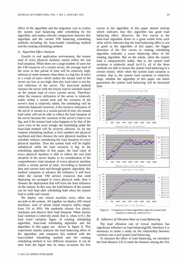
We deploy one virtual machine every other ten

seconds to the system. All together we deploy 100 virtual

machines, each of whose initial resource utility ranges

from 5% to 30%. We randomly choose five physic

machines and observe their load situation. When system load variation is relatively small, that is, when α<0.1, the

load trend variation figure of rotating scheduling

algorithm, least-load scheduling algorithm and the

algorithm of this paper are shown in figure 8. This

experiment mainly analyzes the load balancing effect of

the algorithm, and compares this method with the

least-loaded scheduling method and the rotating

scheduling method in two different situations. It can be

seen from the figure that on many occasions the five

curves in the algorithm of this paper almost overlap

which indicates that this algorithm has good load

balancing effect. However, the five curves in the

least-load algorithm divert to a great extent from each

other which indicates that the load balancing effect is not

as good as the algorithm of this paper; the bigger

diversion of the five curves in rotating scheduling

algorithm indicates a worse balancing effect of the

rotating algorithm. But on the whole, when the system

load is comparatively stable, that is, the system load

variation is relatively small (α<0.1), all of the three methods are able to ensure the system load balancing to a

certain extent; while when the system load variation is

evident, that is, the system load variation is relatively

large, whether the algorithm of this paper can better

guarantees the system load balancing will be discussed

later.

Figure 8. Comparison of three algorithms when the system load

variation is relatively small (α<0.1)

B. Influence of Vibration Rate on Load Balancing

The load vibration rate of virtual machines has

significant influence on load balancing[30], therefore it is

necessary to make a study on the relationship between

variation rate α and system load balancing. To measure the effect of load balancing, we introduce

the load distance LD to mark the distance among the five

Least-Load Scheduling Algorithm

0

10

20

30

40

50

60

70

80

90

100

1 6 11 16 21 26 31 36

Running Time of the System(s)

Load of Physical Machine(%)

PhysicalMachine1PhysicalMachine2PhysicalMachine3PhysicalMachine4PhysicalMachine5

0 500 1000 1500 2000 2500 3000 3500 4000

Algorithm of this paper

0

10

20

30

40

50

60

70

80

90

100

1 6 11 16 21 26 31 36




0 500 1000 1500 2000 2500 3000 3500 4000

Rotating Scheduling Algorithm

0

10

20

30

40

50

60

70

80

90

100

1 6 11 16 21 26 31 36




0 500 1000 1500 2000 2500 3000 3500 4000



curves. At any moment, LD refers to the added distance

between every two points on the five curves. The closer

the five curves, the smaller LD is and the more balanced

the system load is.

Suppose G is the group of all load observation points,

N is the total number of observation points. If P is one

certain point, then the load of five servers observed at

point P are L0，L1，L2，L3，L4. And the load distance LDP

at point P is:

LD𝑃 = |L𝑖 − L𝑗 |4

𝑗=𝑖+1

3

𝑖=0

(14)

We measure the whole load balancing effect by the

average load distance which refers to the mean of the

load distance at all observation points. The computing

formula of this mean is:

LD = LD PP∈G

N (15)

In order to examine the influence of VM load

variation rate α on average load distance, we work out

the correspondent average load distance respectively

when α is 0.1, 0.2, …, 0.9. The result is shown in figure 9.

It indicates that load variation has very little influence on the load balancing effect of the algorithm in this paper; in

contrast, it has bigger influence on least-load algorithm

and the biggest influence on rotating scheduling

algorithm.

Figure 9. Comparison of three algorithms when the system load

variation is relatively changed

C. Migration Cost Analysis

In cloud-computing environment, the resources of a

specific VM provide specific service, such as the specific

software resources and computing resources. However,

the uncertainty of users usually leads to the uncertainty of

the utilization of server resources. Consequently there

will be big variation in the load of every physical machine. And very often the system still needs a dynamic

migration in a period of time to realize load balance after

the scheduling. The scheduling effects of the least-load

method and the method in this paper are relatively

satisfactory when then resources utilization is certain or

rather the variation of the system load is small; and the

migration cost caused by the system variation after

scheduling is low; in contrast, due to its ignorance of the

load situation of the system. The rotation scheduling

method brings high migration cost after scheduling both

when the system load is stable and variant. What is more, since the least-load method only takes into consideration

of the instant load of very server during system

scheduling which is not able to reflect the real load of

physical servers, it will probably lead to the serious

unbalance for the system load after scheduling. The

rotation scheduling method may also lead to the increase

of the system migration cost which means the VM

number will be increased to achieve system load

balancing and the migration cost of the algorithm will be

raised sharply with the increase of the system load

variation. The method in this paper according to

historical data and current state and through genetic algorithm, computes in advance the influence it will have

when the current VM service resources that need

deploying are arranged to every physical node, then

chooses the deployment that will have the least influence

on the system. In this way, the problem of load imbalance

of the system after scheduling can be avoided to a great

extent, and the migration cost after scheduling is reduced

to the lowest level.

On some special occasions, there is a big increase of

the load of some nodes in the system due to frequent

access thus leads to the load imbalance of the whole system. Under this situation, usually the system cannot

realize the system load balancing through only one-time

scheduling so it must do it through VM migration.

However, the cost of VM migration cannot be neglected.

Thus where the VM should be migrated and how to

migrate the least number of VM are also the problems

that need consideration during VM scheduling. The

algorithm of this paper takes historical factors into

consideration. It computes the situation of the whole

system after scheduling in advance through genetic

algorithm and then chooses the scheduling solution with the lowest cost. Figure 10 shows the average VM

migration ratio while the VM load variation rate α is

changing. It can be seen that the method of this paper

shows conspicuous advantage. The experiment shows

that the method of this paper can greatly brings down the

migration cost.

Figure 10. The migration ratio of VM when the number of started VM

is different

D. Utilization Rate of the Algorithm

We investigate the utilization rate of the algorithm in

this paper, Least-loaded, Rotating algorithm and the

average utilization for other queuing and configurable

scheduling. From the Figure 11, we can work out how

much resource each model wasted when allocating

different number of VMs. And we find that sometimes

0

50

100

150

200

250

300

350

400

450

1 2 3 4 5 6 7 8 9

Load Volatility a

Average load distance

Algotithm ofthis paper

Least-loadschedulingalgorithm

Rotatingschedulingalgorithm

0.1 0.2 0.3 0.4 0.5 0.6 0.7 0.8 0.9

0

10

20

30

40

50

60

70

80

90

100

1 3 5 7 9 11 13 15 17 19

The Number of VM Started

The Ratio of VM Migration(%)

Algotithm ofthis paper

Least-loadschedulingalgorithm

Rotatingschedulingalgorithm

5010 20 30 40 60 70 80 9050



the Least-loaded, Rotating and queuing systems cannot

allocate resources for all the VMs even if there are

enough resources for the VMs. But the algorithm in this

paper always gives a good scheduling as long as there are

enough resources. On the other hand, we can see that the

algorithm in this paper saves the most resources.

Figure 11. Comparison of three algorithms for the utilization rate

VIII. CONCLUSIONS

In view of the current load balancing in VM resources

scheduling, this paper presents a scheduling strategy on

VM load balancing based on genetic algorithm.

Considering the VM resources scheduling in cloud

computing environment and with the advantage of

genetic algorithm, this method according to historical data and current states computes in advance the influence

it will have on the whole system when the current VM

service resources that need deploying are arranged to

every physical node, and then it chooses the solution

which will have the least influence on the system after

arrangement. In this way, the method achieves the best

load balancing and reduces or avoids dynamic migration

thus resolves the problem of load unbalancing and high

migration cost caused by traditional scheduling

algorithms. The experimental results show that this

method can better realize load balancing and proper resource utilization.

This paper builds a model based on the concrete

situations of cloud computing. It considers the historical

data and current states of VM, uses tree structure to do

the coding in genetic algorithm, proposes the

correspondent strategies of selection, hybridization and

variation also puts some control on the method so that it

has better astringency. However in real cloud computing

environment, there might be dynamic change in VMs,

and there also might be an increase of computing cost of

virtualization software and some unpredicted load

wastage with the increase of VM number started on every physical machine. Therefore, a monitoring and analyzing

mechanism is needed to better solve the problem of load

balancing. This is also a further research subject.

ACKNOWLEDGMENT

This work is supported by The National "863"

Program of China (Grant No.2009AA01Z142). Thanks

for the support from Platform Corporation and High

Performance Computing center of Northwestern

Polytechnical University.

REFERENCES

[1] Michael Armbrust, Armando Fox, Rean Griffith, Anthony D.

Joseph, Randy Katz, Andy Konwinski, Gunho Lee, David

Patterson, Ariel Rabkin, Ion Stoica, and Matei Zaharia, “Above

the clouds: A berkeley view of cloud computing,” UC Berkeley

Technical Report UCB/EECS-2009-28, February 2009.

[2] Borja Sotomayor, Kate Keahey, and Ian Foster, “Overhead

matters: A model for virtual resource management,” In VTDC '06:

Proceedings of the 1st International Workshop on Virtualization

Technology in Distributed Computing, page 5, Washington, DC,

USA, 2006.

[3] Borja Sotomayor, Kate Keahey, Ian Foster, and Tim Freeman,

“Enabling cost-effective resource leases with virtual machines,”

In Hot Topics session in ACM/IEEE International Symposium on

High Performance Distributed Computing 2007 (HPDC 2007),

2007.

[4] L. Cherkasova, D. Gupta, and A. Vahdat, “When virtual is harder

than real: Resource allocation challenges in virtual machine based

it environments,” Technical Report HPL-2007-25, February 2007.

[5] Clark C, Fraser K, Hand S, “Live Migration of Virtual

Machines[C],” Proceedings of the 2nd Int’l Conference on

Networked Systems Design & Implementation. Berkeley, CA,

USA, 2005.

[6] Wei Wang, “A reliable dynamic scheduling algorithm based on

Bayes trust model,” Computer Science, 2007.

[7] Rewinin H E, Lewis T G, Ali H H, “Task Scheduling in parallel

and Distributed System Englewood Cliffs,” New Jersey: Prentice

Hall, 1994, pp. 401-403.

[8] Wu M, Gajski D, Hypertool, “A programming aid for message

passing system,” IEEE Trans Parallel Distrib Syst, 1990, pp.

330-343.

[9] Hwang J J, Chow Y C, Anger F D, “Scheduling precedence

graphics in systems with inter-processor communication times,”

SIAM J Comput, 1989, pp. 244-257.

[10] Rewinin H E, Lewis T G, “Scheduling parallel programs onto

arbitrary target machines,” J Parallel Distrib Comput, 1990, pp.

138-53.

[11] Sih G C, Lee E A, “A compile-time scheduling heuristic for

Interconnection-constraint heterogeneous processor architectures,”

IEEE Trans Parallel Distrib Syst, 1993, pp. 175-187.

[12] Wood T, “Black-box and Gray-box Strategies for Virtual Machine

Migration[C],” Proceedings of the 4th Int’l Conference on

Networked Systems Design & Implementation, IEEE Press, 2007.

[13] VMWare, “VMware DRS - Dynamic Scheduling of System

Resources,” http://www.vmware.com/cn/products/vi/vc/drs.html,

2009.

[14] D. Nurmi, R. Wolski, C. Grzegorczyk, G. Obertelli, S. So-man, L.

Youseff, and D. Zagorodnov, “ The Eucalyptus open-source

cloud-computing system”, IEEE International Symposium on

Cluster Computing and the Grid (CCGrid ’09), 2009.

[15] OpenNebula, “OpenNebula Software,”

http://www.opennebula.org, 2010.

[16] Nimbus, http://nimbusproject.org, 2010.

[17] E. Goldberg, “The existential pleasures of genetic algorithms,” In:

Genetic Algorithms in Engineering and Computer Science, Winter

G ed. New York: Wiley, 1995, pp. 23-31.

[18] Kim, H. Kim, M. Jeon, E. Seo, J. Lee, “Guest-aware prioritybased

virtual machine scheduling for highly consolidated server,” In

Proc. Euro-Par, 2008.

[19] Ongaro, A. L. Cox, and S. Rixner, “Scheduling I/O in virtual

machine monitors,” In Proc. VEE, 2008.

[20] L. Cherkasova, D. Gupta, and A. Vahdat, “Comparison of the

three CPU schedulers in Xen,” SIGMETRICS Perform. Eval.

Rev., 2007, pp. 42–51.

0

20

40

60

80

100

1 2 3 4 5 6

The Number of Started VM

Utilization Rate(%)

GA Algorithm Least-loaded Rotating Average

5

0

0

20 40 60 80 100



[21] Hu Jinhua, Gu Jianhua, Sun Guofei, Zhao Tianhai. A Scheduling

Strategy on Load Balancing of Virtual Machine Resources in

Cloud Computing Environment, PAAP2010, 2010, pp. 89-96.

[22] Hai Zhong, Kun Tao, Xuejie Zhang, “An Approach to Optimized

Resource Scheduling Algorithm for Open-source Cloud Systems”,

The Fifth Annual ChinaGrid Conference, 2010.

[23] T. Tan and C. Kiddle, “An Assessment of Eucalyptus Version

1.4”, Technical Report 2009-928-07, Department of Computer

Science, University of Calgary, 2009.

[24] Haizea, http://haizea.cs.uchicago.edu, 2010.

[25] Amazon Web Services, http://aws.amazon.com, 2010.

[26] openPBS, http://pbsgridworks.com, 2010.

[27] SunGridEngine, http://gridengine.sunsource.net, 2010.

[28] Yunzhu Ni, Guanghong Lv, Yanhui Huang, “The Solution of Disk

Load Balancing Based on Disk Striping with Geneti Algorithm,”

Chinese Journal of Computers, 2006.

[29] Platform, “Platform ISF Software”, http://www.platform.com.cn/,

2010.

[30] Li WZ, Guo S, Xu P, Lu SL, Chen DX．An adaptive load

balancing algorithm for service composition．Journal ofSoftware，

2006，17(5)：1068—1077.

BIOGRAPHIES

Jianhua Gu, Male, Doctor, Professor, Doctor Supervisor,

Specialized in Distributed Computing, High Performance

Computing

Jinhua Hu, Male, Master, Specialized in Distributed

Computing

Tianhai Zhao, Male, Doctor, Instructor, Specialized in

Distributed Computing, High Performance Computing

Guofei Sun, Male, Master, Specialized in Distributed

Computing



a new resource scheduling strategy based on genetic algorithm in cloud computing environment

Documents