A Nonstandard Derivation for the Special Theory of Relativity*

Robert A. Herrmann

Mathematics DepartmentU. S. Naval Academy572C Holloway Rd

Annapolis, MD 21402-5002 USA21 SEP 1993, last revision 25 APR 2010.

Abstract: Using properties of the nonstandard physical world, a new

fundamental derivation for all of the effects of the Special Theory of

Relativity is given. This fundamental derivation removes all the con-

tradictions and logical errors in the original derivation and leads to the

fundamental expressions for the Special Theory Lorentz transformations.

Necessary, these are obtained by means of hyperbolic geometry. It is

shown that the Special Theory effects are manifestations of the inter-

action between our natural world and a nonstandard photon-particle

medium (NSPPM). This derivation eliminates the controversy associ-

ated with any physically unexplained absolute time dilation and length

contraction. It is shown that there is no such thing as a absolute time

dilation and length contraction but, rather, alterations in pure numerical

quantities associated with interactions with the NSPPM.

1. The Fundamental Postulates.

There are various Principles of Relativity. The most general and least justifiedis the one as stated by Dingle “There is no meaning in absolute motion. By sayingthat such motion has no meaning, we assert that there is no observable effect bywhich we can determine whether an object is absolutely at rest or in motion, orwhether it is moving with one velocity or another.”[1:1] Then we have Einstein’sstatements that “I. The laws of motion are equally valid for all inertial framesof reference. II. The velocity of light is invariant for all inertial systems, beingindependent of the velocity of its source; more exactly, the measure of this velocity(of light) is constant, c, for all observers.”[7:6–7] I point out that Einstein’s originalderivation in his 1905 paper (Ann. der Phys. 17: 891) uses certain well-knownprocesses related to partial differential calculus.

In 1981 [5] and 1991 [2], it was discovered that the intuitive concepts asso-ciated with the Newtonian laws of motion were inconsistent with respect to themathematical theory of infinitesimals when applied to a theory for light propaga-tion. The apparent nonballistic nature for light propagation when transferred toinfinitesimal world would also yield a nonballistic behavior. Consequently, there is

*This is an expanded version of the paper: Herrmann, R. A., Special relativityand a nonstandard substratum, Speculat. Sci. Technol., 17(1994), 2-10.

1

an absolute contradiction between Einstein’s postulate II and the deriva-tion employed. This contradiction would not have occurred if it had not beenassumed that the æther followed the principles of Newtonian physics with respectto electromagnetic propagation. [Note: On Nov. 14, 1992, when the informationin this article was formally presented, I listed various predicates that Einstein usedand showed the specific places within the derivations where the predicate’s domainwas altered without any additional argument. Thus, I gave specific examples of themodel theoretic error of generalization. See page 49.]

I mention that Lorentz speculated that æther theory need not correspond di-rectly to the mathematical structure but could not show what the correct corre-spondence would be. Indeed, if one assumes that the NSPPM satisfies the mostbasic concept associated with an inertial system that a body can be considered ina state of rest or uniform motion unless acted upon by a force, then the expressionF = ma, among others, may be altered for infinitesimal NS-substratum behavior.Further, the NS-substratum, when light propagation is discussed, does not followthe Galilean rules for velocity composition. The additive rules are followed but nonegative real velocities exterior to the Euclidean monads are used since we are onlyinterested in the propagation properties for electromagnetic radiation. The deriva-tion in section 3 removes all contradictions by applying the most simplistic Galileanproperties of motion, including the ballistic property, but only to behavior withina Euclidean monad.

As discussed in section 3, the use of an NSP-world (i.e. nonstandard phys-

ical world) NSPPM allows for the elimination of the well-known Special Theory“interpretation” contradiction that the mathematical model uses the concepts ofNewtonian absolute time and space, and, yet, one of the major interpretations isthat there is no such thing as absolute time or absolute space.

Certain general principles for NSPPM light propagation will be specificallystated in section 3. These principles can be gathered together as follows: (1) Thereis a portion of the nonstandard photon-particle medium - the NSPPM - that sus-tains N-world (i.e. natural = physical world) electromagnetic propagation. Suchpropagation follows the infinitesimally presented laws of Galilean dynamics, whenrestricted to monadic clusters, and the monadic clusters follow an additive and anactual metric property for linear relative motion when considered collectively. [Theterm “nonstandard electromagnetic field” should only be construed as a NSPPMnotion, where the propagation of electromagnetic radiation follows slightly differentprinciples than within the natural world.] (2) The motion of light-clocks withinthe N-world (natural world) is associated with one single effect. This effect is analteration in an appropriate light-clock mechanism. [The light-clock concept willbe explicitly defined at the end of section 3.] It will be shown later that an actualphysical cause may be associated with vreified Special Theory physical alterations.Thus the Principle of Relativity, in its general form, and the inconsistent portionsof the Einstein principles are eliminated from consideration and, as will be shown,the existence of a special type of medium can be assumed without contradicting

2

experimental evidence.

In modern Special Theory interpretations [6], it is claimed that the effect of“length contraction” has no physical meaning, whereas time dilation does. This isprobably true if, indeed, the Special Theory is actually based upon the intrinsicN-world concepts of length and time. What follows will further demonstrate thatthe Special Theory is a light propagation theory, as has been previously arguedby others, and that the so-called “length contraction” and time dilation can bothbe interpreted as physically real effects when they are described in terms of theNSPPM. The effects are only relative to a theory of light propagation.

2. Pre-derivation Comments.

Recently [2]–[4], nonstandard analysis [8] has proved to be a very significanttool in investigating the mathematical foundations for various physical theories. In1988 [4], we discussed how the methods of nonstandard analysis, when applied tothe symbols that appear in statements from a physical theory, lead formally to apregeometry and the entities termed as subparticles. One of the goals of NSP-worldresearch is the re-examination of the foundations for various controversial N-worldtheories and the eventual elimination of such controversies by viewing such theoriesas but restrictions of more simplistic NSP-world concepts. This also leads to indirectevidence for the actual existence of the NSP-world.

The Special Theory of Relativity still remains a very controversial theory due toits philosophical implications. Prokhovnik [7] produced a derivation that yields all ofthe appropriate transformation formulas based upon a light propagation theory, butunnecessarily includes an interpretation of the so-called Hubble textural expansionof our universe as an additional ingredient. The new derivation we give in thisarticle shows that properties of a NSPPM also lead to Prokhovnik’s expression(6.3.2) in reference [7] and from which all of the appropriate equations can bederived. However, rather than considering the Hubble expansion as directly relatedto Special Relativity, it is shown that one only needs to consider simplistic NSP-world behavior for light propagation and the measurement of time by means ofN-world light-clocks. This leads to the conclusion that Special Theory effects maybe produced by a dense NSPPM within the NSP-world. Such an NSPPM – anæther – yields N-world Special Theory effects.

3. The derivation

The major natural system in which we exist locally is a space-time system.“Empty” space-time has only a few characterizations when viewed from an Eu-clidean perspective. We investigate, from the NSP-world viewpoint, electromag-netic propagation through a Euclidean neighborhood of space-time. Further, weassume that light is such a propagation. One of the basic precepts of infinitesimalmodeling is the experimentally verified simplicity for such a local system. For ac-tual time intervals, certain physical processes take on simplistic descriptions. TheseNSP-world descriptions are represented by the exact same description restricted to

3

infinitesimal intervals. Let [a, b], a 6= b, a > 0, be an objectively real conceptionaltime interval and let t ∈ (a, b).

The term “time” as used above is very misunderstood. There are variousviewpoints relative to its use within mathematics. Often, it is but a term used inmathematical modeling, especially within the calculus. It is a catalyst so to speak.It is a modeling technique used due to the necessity for infinitesimalizing physicalmeasures. The idealized concept for the “smoothed out” model for distance measureappears acceptable. Such an acceptance comes from the use of the calculus in suchareas as quantum electrodynamics where it has great predictive power. In thesubatomic region, the assumption that geometric measures have physical meaning,even without the ability to measure by external means, is justified as an appropriatemodeling technique. Mathematical procedures applied to regions “smaller than”those dictated by the uncertainty principle are accepted although the reality of theinfinitesimals themselves need not be assumed. On the other hand, for this modelingtechnique to be applied, the rules for ideal infinitesimalizing should be followed.

The infinitesimalizing of ideal geometric measures is allowed. But, with respectto the time concept this is not the case. Defining measurements of time as repre-sented by the measurements of some physical periodic process is not the definitionupon which the calculus is built. Indeed, such processes cannot be infinitesimalized.To infinitesimalize a physical measurement using physical entities, the entities beingobserved must be capable of being smoothed out in an ideal sense. This means thatonly the macroscopic is considered, the atomic or microscopic is ignored. Underthis condition, you must be able to subdivide the device into “smaller and smaller”pieces. The behavior of these pieces can then be transferred to the world of the in-finitesimals. Newton based the calculus not upon geometric abstractions but uponobservable mechanical behavior. It was this mechanical behavior that Newton usedto define physical quantities that could be infinitesimalized. This includes the defi-nition of “time.”

All of Newton’s ideas are based upon velocities as the defining concept. Thenotation that uniform (constant) velocity exists for an object when that object isnot affected by anything, is the foundation for his mechanical observations. Thisis an ideal velocity, a universal velocity concept. The modern approach would beto add the term “measured” to this mechanical concept. This will not changethe concept, but it will make it more relative to natural world processes and arequired theory of measure. This velocity concept is coupled with a smoothed outscale, a ruler, for measurement of distance. Such a ruler can be infinitesimalized.From observation, Newton then infinitesimalized his uniform velocity concept. Thisproduces the theory of fluxions.

Where does observer time come into this picture? It is simply a defined quantitybased upon the length and velocity concept. Observationally, it is the “thing” wecall time that has passed when a test particle with uniform velocity first crosses apoint marked on a scale and then crosses a second point marked on the same scale.This is in the absence of any physical process that will alter either the constantvelocity or the scale. Again this definition would need to be refined by inserting the

4

word “measured.” Absolute time is the concept that is being measured and cannotbe altered as aconcept.

Now with Einstein relativity, we are told that measured quantities are effectedby various physical processes. All theories must be operational in that the conceptof measure must be included. But, the calculus is used. Indeed, used by Einsteinin his original derivation. Thus, unless there is an actual physical entity that canbe substituted for the Newton’s ideal velocity, then any infinitesimalizing processwould contradict the actual rules of application of the calculus to the most basic ofphysical measures. But, the calculus is used to calculate the measured quantities.Hence, we are in a quandary. Either there is no physical basis for mathematicalmodels based upon the calculus, and hence only selected portions can be realizedwhile other selected portions are simply parameters not related to reality in anymanner, or the calculus is the incorrect mathematical structure for the calculations.Fortunately, nature has provided us with the answer as to why the calculus, whenproperly interpreted, remains such a powerful tool to calculate the measures thatdescribe observed physical behavior.

In the 1930s, it was realized that the measured uniform velocity of the to-and-fro velocity of electromagnetic radiation, (i.e. light) is the only known natural entitythat will satisfy the Newtonian requirements for an ideal velocity and the conceptsof space-time and from which the concept of time itself can be defined. The firstto utilize this in relativity theory was Milne. This fact I learned after the firstdraughts of this paper were written and gives historical verification of this paper’sconclusions. Although, it might be assumed that such a uniform velocity conceptas the velocity of light or light paths in vacuo cannot be infinitesimalized, this isnot the case. Such infinitesimalizing occurs for light-clocks and from the simpleprocess of “scale changing” for a smoothed out ruler. What this means is that, atits most basic physical level, conceptually absolute or universal Newton time canhave operational meaning as a physical foundation for a restricted form of “time”that can be used within the calculus.

As H. Dingle states it, “The second point is that the conformability of light toNewton mechanics . . . makes it possible to define corresponding units of space andtime in terms of light instead of Newton’s hypothetical ‘uniformly moving body.’ ”[The Relativity of Time, Nature, 144(1939): 888–890.] It was Milne who first (1933)attempted, for the Special Theory, to use this definition for a “Kinematic Relativity”[Kinematic Relativity, Oxford University Press, Oxford, 1948] but failed to extendit successfully to the space-time environment. In what follows such an operationaltime concept is being used and infinitesimalized. It will be seen, however, thatbased upon this absolute time concept another time notion is defined, and thisis the actual time notion that must be used to account for the physical changesthat seem to occur due to relativistic processes. In practice, the absolute time iseliminated from the calculations and is replaced by defined “Einstein time.” It isshown that Einstein time can be infinitesimalized through the use of the definable“infinitesimal light-clocks” and gives an exact measurement.

Our first assumption is based entirely upon the logic of infinitesimal analysis,

5

reasoning, modeling and subparticle theory.

(i) “Empty” space within our universe, from the NSP-worldviewpoint, is composed of a dense-like nonstandard medium (theNSPPM) that sustains, comprises and yields N-world Special The-ory effects. These NSPPM effects are electromagnetic in character.

This medium through which the effects appear to propagate comprise the objectsthat yield these effects. The next assumption is convincingly obtained from a simpleand literal translation of the concept of infinitesimal reasoning.

(ii) Any N-world position from or through which an electromag-netic effect appears to propagate, when viewed from the NSP-world, is embedded into a disjoint “monadic cluster” of theNSMP, where this monadic cluster mirrors the same unusual or-der properties, with respect to propagation, as the nonstandardordering of the nonarchimedian field of hyperreal numbers ∗

IR. [2]A monadic cluster may be a set of NS-substratum subparticleslocated within a monad of the standard N-world position. Thepropagation properties within each such monad are identical.

In what follows, consider two (local) fundamental pairs of N-world positionsF1, F2 that are in nonzero uniform (constant) NSP-world linear and relative mo-tion. Our interest is in what effect such nonzero velocity might have upon suchelectromagnetic propagation. Within the NSP-world, this uniform and linear mo-tion is measured by the number w that is near to a standard number ω and thisvelocity is measured with respect to conceptional NSP-world time and a stationarysubparticle field. [Note that field expansion can be additionally incorporated.] Thesame NSP-world linear ruler is used in both the NSP-world and the N-world. Theonly difference is that the ruler is restricted to the N-world when such measurementsare made. N-world time is measured by only one type of machine – the light-clock.The concept of the light-clock is to be considered as any clock-like apparatus thatutilizes either directly or indirectly an equivalent process. As it will be detailed,due to the different propagation effects of electromagnetic radiation within the two“worlds,” measured N-world light-clock time need not be the same as the NSP-world time. Further, the NSP-world ruler is the measure used to define the N-worldlight-clock.

Experiments show that for small time intervals [a, b] the Galilean theory ofaverage velocities (velocitys) suffices to give accurate information relative to thecompositions of such velocities. Let there be an internal function q: ∗ [a, b] → ∗

IR,where q represents in the NSP-world a distance function. Also, let nonnegative andinternal `: ∗ [a, b] → ∗

IR be a function that yields the NSP-world velocity of theelectromagnetic propagation at any t ∈ ∗ [a, b]. As usual µ(t) denotes the monad ofstandard t, where “t” is an absolute NSP-world “time” parameter.

The general and correct methods of infinitesimal modeling state that, within theinternal portion of the NSP-world, two measures m1 and m2 are indistinguishable for

6

dt (i.e. infinitely close of order one) (notation m1 ∼ m2) if and only if 0 6= dt ∈ µ(0),(µ(0) the set of infinitesimals)

m1

dt− m2

dt∈ µ(0). (3.1)

Intuitively, indistinguishable in this sense means that, although within the NSP-world the two measures are only equivalent and not necessarily equal, the first level

(or first-order) effects these measures represent over dt are indistinguishable withinthe N-world (i.e. they appear to be equal.)

In the following discussion, we continue to use photon terminology. Within theN-world our photons need not be conceived of as particles in the sense that thereis a nonzero finite N-world distance between individual photons. Our photons may

be finite combinations of intermediate subparticles that exhibit, when the standardpart operator is applied, basic electromagnetic field properties. They need notbe discrete objects when viewed from the N-world, but rather they could just aswell give the appearance of a dense NS-substratum. Of course, this dense NSPPMportion is not the usual notion of an “æther” (i.e. ether) for it is not a subset ofthe N-world. This dense-like portion of the NS-substratum containsnonstandard

particle medium (NSPPM). Again “photon” can be considered as but a convenientterm used to discuss electromagnetic propagation. Now for another of our simplisticphysical assumptions.

(iii) In an N-world convex space neighborhood I traced out over thetime interval [a, b], the NSPPM disturbances appear to propagatelinearly.

As we proceed through this derivation, other such assumptions will be identified.The functions q, ` need to satisfy some simple mathematical characteristic.

The best known within nonstandard analysis is the concept of S-continuity [8]. So,where defined, let q(x)/x (a velocity type expression) and ` be S-continuous, and` limited (i.e. finite) at each p ∈ [a, b], (a+ at a, b− at b). From compactness,q(x)/x and ` are S-continuous, and ` is limited on ∗ [a, b]. Obviously, both q and` may have infinitely many totally different NSP-world characteristics of which wecould have no knowledge. But the function q represents within the NSP-world thedistance traveled with linear units by an identifiable NSPPM disturbance. But thefunction q represents, within the NSP-world, the distance traveled with linear unitsby an identifiable NSPPM disturbance. The notion of“lapsed-time” is used. Thex 6= 0 is the lapsed-time between two events. It follows from all of this that for eacht ∈ [a, b] and t′ ∈ µ(t) ∩ ∗ [a, b],

q(t′)

t′− q(t)

t∈ µ(0); `(t′)− `(t) ∈ µ(0). (3.2)

Expressions (3.2) give relations between nonstandard t′ ∈ µ(t) and the standard t.Recall that if x, y ∈ ∗

IR, then x ≈ y iff x− y ∈ µ(0).

7

From (3.2), it follows that for each dt ∈ µ(0) such that t + dt ∈ µ(t) ∩ ∗ [a, b]

q(t + dt)

t + dt≈ q(t)

t, (3.3)

`(t + dt) +q(t + dt)

t + dt≈ `(t) +

q(t)

t. (3.4)

From (3.4), we have that(

`(t + dt) +q(t + dt)

t + dt

)

dt ∼(

`(t) +q(t)

t

)

dt. (3.5)

It is now that we begin our application of the concepts of classical Galileancomposition of velocities but restrict these ideas to the NSP-world monadic clus-ters and the notion of indistinguishable effects. You will notice that within theNSP-world the transfer of the classical concept of equality of constant or averagequantities is replaced by the idea of indistinguishable. At the moment t ∈ [a, b] thatthe standard part operator is applied, an effect is transmitted through the NSPPMas follows:

(iv) For each dt ∈ µ(0) and t ∈ [a, b] such that t + dt ∈ ∗ [a, b],the NSP-world distance q(t + dt) − q(t) (relative to dt) traveledby the NSPPM effect within a monadic cluster is indistinguishablefor dt from the distance produced by the Galilean composition ofvelocities.

From (iv), it follows that

q(t + dt)− q(t) ∼(

`(t + dt) +q(t + dt)

t + dt

)

dt. (3.6)

And from (3.5),

q(t + dt)− q(t) ∼(

`(t) +q(t)

t

)

dt. (3.7)

Expression (3.7) is the basic result that will lead to conclusions relative to theSpecial Theory of Relativity. In order to find out exactly what standard functionswill satisfy (3.7), let arbitrary t1 ∈ [a, b] be the standard time at which electromag-netic propagation begins from position F1. Next, let q = ∗s be an extended standardfunction and s is continuously differentiable on [a, b]. Applying the definition of ∼,yields

∗s(t + dt)− s(t)

dt≈ `(t) +

s(t)

t. (3.8)

Note that ` is microcontinuous on ∗ [a, b]. For each t ∈ [a, b], the value `(t) islimited. Hence, let st(`(t)) = v(t) ∈ IR. From Theorem 1.1 in [3] or 7.6 in [10], v iscontinuous on [a, b]. [See note 1 part a.] Now (3.8) may be rewritten as

∗

(

d(s(t)/t)

dt

)

=∗v(t)

t, (3.9)

8

where all functions in (3.9) are *-continuous on ∗ [a, b]. Consequently, we may applythe *-integral to both sides of (3.9). [See note 1 part b.] Now (3.9) implies that fort ∈ [a, b]

s(t)

t= ∗

∫ t

t1

∗v(x)

xdx, (3.10)

where, for t1 ∈ [a, b], s(t1) has been initialized to be zero.Expression (3.10) is of interest in that it shows that although (iv) is a simplistic

requirement for monadic clusters and the requirement that q(x)/x be S-continuousis a customary property, they do not lead to a simplistic NSP-world function, evenwhen view at standard NSP-world times. It also shows that the light-clock assump-tion was necessary in that the time represented by (3.10) is related to the distancetraveled and unknown velocity of an identifiable NSPPM disturbance. It is alsoobvious that for pure NSP-world times the actual path of motion of such propaga-tion effects is highly nonlinear in character, although within a monadic cluster thedistance ∗s(t + dt)− s(t) is indistinguishable from that produced by the linear-likeGalilean composition of velocities.

Further, it is the standard function in (3.10) that allows us to cross over toother monadic clusters. Thus, substituting into (3.7) yields, since the propagationbehavior in all monadic clusters is identical,

∗s(t + dt)− s(t) ∼(

∗v(t) +(

∗∫ t

t1∗v(x)/xdx

))

dt, (3.11)

for every t ∈ [a, b], t + dt ∈ µ(t) ∩ ∗ [a, b]

Consider a second standard position F2 at which electromagnetic reflectionoccurs at t2 ∈ [a, b], t2 > t1, t2 + dt ∈ µ(t2) ∩ ∗ [a, b]. Then (3.11) becomes

∗s(t2 + dt)− s(t2) ∼(

∗v(t2) +(

∗∫ t2t1

∗v(x)/xdx))

dt. (3.12)

Our final assumption for monadic cluster behavior is that the classical ballisticproperty holds with respect to electromagnetic propagation.

(v) From the exterior NSP-world viewpoint, at standard time t ∈[a, b], the velocity ∗v(t) acquires an additional velocity w.

Applying the classical statement (v), with the indistinguishable concept, meansthat the distance traveled ∗s(t2+dt)−s(t2) is indistinguishable from ( ∗v(t2)+w)dt.Hence,

( ∗v(t2) + w)dt ∼ ∗s(t2 + dt)− s(t2) ∼(

∗v(t2) +

(

∗

∫ t2

t1

∗v(x)

xdx

))

dt. (3.13)

Expression (3.13) implies that

∗v(t2) + w ≈ ∗v(t2) +

(

∗

∫ t2

t1

∗v(x)

xdx

)

. (3.14)

9

Since st(w) is a standard number, (3.14) becomes after taking the standard partoperator,

st(w) = st

(

∗

∫ t2

t1

∗v(x)

xdx

)

. (3.15)

After reflection, a NSPPM disturbance returns to the first position F1 arrivingat t3 ∈ [a, b], t1 < t2 < t3. Notice that the function s does not appear in equation(3.15). Using the nonfavored position concept, a reciprocal argument entails that

s1(t3)

t3= st

(

∗

∫ t3

t2

∗v1(x)

xdx

)

, (3.16)

st(w) = st

(

∗

∫ t3

t2

∗v1(x)

xdx

)

, (3.17)

where s1(t2) is initialized to be zero. It is not assumed that ∗v1 = ∗v.We now combine (3.10), (3.15), (3.16), (3.17) and obtain an interesting non-

monadic view of the relationship between distance traveled by an NSPPM distur-bance and relative velocity.

s1(t3)− s(t2) = st(w)(t3 − t2). (3.18)

Although reflection has been used to determine relation (3.18) and a linear-likeinterpretation involving reflection seems difficult to express, there is a simple non-reflection analogue model for this behavior.

Suppose that a NSPPM disturbance is transmitted from a position F1, to aposition F2. Let F1 and F2 have no NSP-world relative motion. Suppose that aNSPPM disturbance is transmitted from F1 to F2 with a constant velocity v withthe duration of the transmission t′′ − t′, where the path of motion is considered aslinear. The disturbance continues linearly after it passes point F2 but has increasedduring its travel through the monadic cluster at F2 to the velocity v + st(w). Thedisturbance then travels linearly for the same duration t′′− t′. The linear differencein the two distances traveled is w(t′′ − t′). Such results in the NSP-world should beconstrued only as behavior mimicked by the analogue NSPPM model.

Equations (3.10) and (3.15) show that in the NSP-world NSPPM disturbancespropagate. Except for the effects of material objects, it is assumed that in the N-world the path of motion displayed by a NSPPM disturbance is linear. This includesthe path of motion within an N-world light-clock. We continue this derivation basedupon what, at present, appears to be additional parameters, a private NSP-worldtime and an NSP-world rule. Of course, the idea of the N-world light-clock is beingused as a fixed means of identifying the different effects the NSPPM is havingupon these two distinct worlds. A question yet to be answered is how can wecompensate for differences in these two time measurements, the NSP-world privatetime measurement of which we can have no knowledge and N-world light-clocks.

10

The weighted mean value theorem for integrals in nonstandard form, whenapplied to equations (3.15) and (3.17), states that there are two NSP-world timesta, tb ∈ ∗ [a, b] such that t1 ≤ ta ≤ t2 ≤ tb ≤ t3 and

st(w) = st( ∗v(ta))

∫ t2

t1

1

xdx = st( ∗v1(tb))

∫ t3

t2

1

xdx. (3.19)

[See note 1 part c.] Now suppose that within the local N-world an F1 → F2, F2 → F1

light-clock styled measurement for the velocity of light using a fixed instrumentationyields equal quantities. (Why this is the case is established in Section 6.) Modelthis by (*) st( ∗v(ta)) = st( ∗v1(tb)) = c in the NSPPM. I point out that there aremany nonconstant *-continuous functions that satisfy property (*). For example,certain standard nonconstant linear functions and nonlinear modifications of them.Property (*) yields

∫ t2

t1

1

xdx =

∫ t3

t2

1

xdx. (3.20)

And solving (3.20) yields

ln

(

t2t1

)

= ln

(

t3t2

)

. (3.21)

From this one hast2 =

√t1t3. (3.22)

Expression (3.22) is Prokhovnik’s equation (6.3.3) in reference [7]. However,(6.3.3) is based upon an ad hoc derivative assumption. Further, the interpretationof this result and the others that follow cannot, for the NSP-world, be those asproposed by Prokhovnik. The times t1, t2, t3, are standard NSPPM times. Further,it is not logically acceptable when considering how to measure such time in the NSP-world or N-world to consider just any mode of measurement. The mode of lightvelocity measurement must be carried out within the confines of the language usedto obtain this derivation. Using this language, a method for time calculation that ispermissible in the N-world is the light-clock method. Any other described methodfor time calculation should not include significant terms from other sources. Timeas expressed in this derivation is not a mystical absolute something or other. It is ameasured quantity based entirely upon some mode of measurement.

They are two major difficulties with most derivations for expressions used inthe Special Theory. One is the above mentioned absolute time concept. The otheris the ad hoc nonderived N-world relative velocity. In this case, no consideration isgiven as to how such a relative velocity is to be measured so that from both F1 andF2 the same result would be obtained. It is possible to achieve such a measurementmethod because of the logical existence of the NSPPM.

In a physical-like sense, the “times” can be considered as the numerical val-ues recorded by single device stationary in the NSPPM. It is conceptual time inthat, when events occur, then such numerical event-times “exist.” It is the not yet

11

identified NSPPM properties that yield the unusual behavior indicated by (3.22).One can use light-clocks and a counter that indicates, from some starting count, thenumber of times the light pulse has traversed back and forth between the mirrorand source of our light-clock. Suppose that F1 and F2 can coincide. When theydo coincide, the F2 light-clock counter number that appears conceptually first afterthat moment can be considered to coincide with the counter number for the F1

light-clock.

After F2 is perceived to no longer coincide with F1, a light pulse is transmittedfrom F1 towards F2 in an assumed linear manner. The “next” F1 counter numberafter this event is τ11. We assume that the relative velocity of F2 with respect toF1 may have altered the light-clock counter numbers, compared to the count at F1,for a light-clock riding with F2. The length L used to define a light-clock is mea-sured by the NSP-world ruler and would not be altered. Maybe the light velocityc, as produced by the standard part operator, is altered by N-world relative veloc-ity. Further, these two N-world light-clocks are only located at the two positionsF1, F2, and this light pulse is represented by a NSPPM disturbance. The lightpulse is reflected back to F1 by a mirror similar to the light-clock itself. The firstcounter number on the F2 light-clock to appear, intuitively, “after” this reflectionis approximated by τ21. The F1 counter number first perceived after the arrival ofthe returning light pulse is τ31.

From a linear viewpoint, at the moment of reflection, denoted by τ21, the pulsehas traveled an operational linear light-clock distance of (τ21−τ11)L. After reflection,under our assumptions and nonfavored position concept, a NSPPM disturbancewould trace out the same operational linear light-clock distance measured by (τ31−τ21)L. Thus the operational light-clock distance from F1 to F2 would be at themoment of operational reflection, under our linear assumptions, 1/2 the sum of thesetwo distances or S1 = (1/2)(τ31−τ11)L. Now we can also determine the appropriateoperational relation between these light-clock counter numbers for S1 = (τ21−τ11)L.Hence, τ31 = 2τ21 − τ11, and τ21 operationally behaves like an Einstein measure.

After, measured by light-clock counts, the pulse has been received back to F1,a second light pulse (denoted by a second subscript of 2) is immediately sent to F2.Although τ31 ≤ τ12, it is assumed that τ31 = τ12 [See note 2.5]. The same analy-sis with new light-clock count numbers yields a different operational distance S2 =(1/2)(τ32−τ12)L and τ32 = 2τ22−τ12. One can determine the operational light-clocktime intervals by considering τ22−τ21 = (1/2)((τ32−τ31)+(τ12−τ11)) and the opera-tional linear light-clock distance difference S2−S1 = (1/2)((τ32−τ31)−(τ12−τ11))L.Since we can only actually measure numerical quantities as discrete or terminatingnumbers, it would be empirically sound to write the N-world time intervals for thesescenarios as t1 = τ12 − τ11, t3 = (τ32 − τ31). This yields the operational Einsteinmeasure expressions in (6.3.4) of [7] as τ22 − τ21 = tE and operational light-lengthrE = S2 − S1, using our specific light-clock approach. This allows us to define,operationally, the N-world relative velocity as vE = rE/tE. [In this section, thet1, t3 are not the same Einstein measures, in form, as described in [7]. But, in sec-

12

tion 4, 5, 6 these operational measures are used along with infinitesimal light-clockcounts to obtain the exact Einstein measure forms for the time measure. This is:the t1 is a specific starting count and the t3 is t1 plus an appropriate lapsed time.]

Can we theoretically turn the above approximate operational approach fordiscrete N-world light-clock time into a time continuum? Light-clocks can be con-sidered from the NSP-world viewpoint. In such a case, the actual NSP-world lengthused to form the light-clock might be considered as a nonzero infinitesimal. Thus,at least, the numbers τ32, τ21, τ31, τ22 are infinite hyperreal numbers, various dif-ferences would be finite and, after taking the standard part operator, all of theN-world times and lengths such as tE, rE , S1, S2 should be exact and not approx-imate in character. These concepts will be fully analyzed in section 6. Indeed, aspreviously indicated, for all of this to hold the velocity c cannot be measured by anymeans. As indicated in section 6, the actual numerical quantity c as it appears in(3.22) is the standard part of pure NSP-world quantities. Within the N-world, oneobtains an “apparent” constancy for the velocity of light since, for this derivation,it must be measured by means of a to-and-fro light-clock styled procedure with afixed instrumentation.

As yet, we have not discussed relations between N-world light-clock measure-ments and N-world physical laws. It should be self-evident that the assumed linear-ity of the light paths in the N-world can be modeled by the concept of projectivegeometry. Relative to the paths of motion of a light path in the NSP-world, theNSPPM disturbances, the N-world path behaves as if it were a projection upon aplane. Prokhovnik analyzes such projective behavior and comes to the conclusionsthat in two or more dimensions the N-world light paths would follow the rules ofhyperbolic geometry. In Prokhovnik, the equations (3.22) and the statements es-tablishing the relations between the operational or exact Einstein measures tE , rE

and vE lead to the Einstein expression relating the light-clock determined relativevelocities for three linear positions having three NSP-world relative and uniformvelocities w1, w2, w3.

In the appendix, in terms of light-clock determined Einstein measures andbased upon the projection idea, the basic Special Theory coordinate transforma-tion is correctly obtained. Thus, all of the NSP-world times have been removedfrom the results and even the propagation differences with respect to light-clockmeasurements. Just use light-clocks in the N-world to measure all these quantitiesin the required manner and the entire Special Theory is forthcoming.

I mention that it can be shown that w and c may be measured by probes thatare not N-world electromagnetic in character. Thus w need not be obtained in thesame manner as is vE except that N-world light-clocks would be used for N-worldtime measurements. For this reason, st(w) = ω is not directly related to the so-called textual expansion of the space within our universe. The NSPPM is not to betaken as a nonstandard translation of the Maxwell EMF equations.

13

4. The Time Continuum.

With respect to models that use the classical continuum approach (i.e. variablesare assumed to vary over such things as an interval of real numbers) does themathematics perfectly measure quantities within nature – quantities that cannotbe perfectly measured by a human being? Or is the mathematics only approximatein some sense? Many would believe that if “nature” is no better than the humanbeing, then classical mathematics is incorrect as a perfect measure of natural systembehavior. However, this is often contradicted in the limit. That is when individualsrefine their measurements, as best as it can done at the present epoch, then thediscrete human measurements seem to approach the classical as a limit. Continuedexploration of this question is a philosophical problem that will not be discussed inthis paper, but it is interesting to model those finite things that can, apparently, beaccomplished by the human being, transfer these processes to the NSP-world andsee what happens. For what follows, when the term “finite” (i.e. limited) hyperrealnumber is used, since it is usually near to a nonzero real number, it will usuallyrefer to the ordinary nonstandard notion of finite except that the infinitesimals havebeen removed. This allows for the existence of finite multiplicative inverses.

First, suppose that tE = st(tEa), rE = st(rEa), S1 = st(S1a), S2 = st(S2a)and each is a nonnegative real number. Thus tEa, rEa, S1a, S2a are all nonnegativefinite hyperreal numbers. Let L = 1/10ω > 0, ω ∈ IN

+∞

. By transfer and the resultthat S1a, S2a, are considered finite (i.e. near standard), then S1a ≈ (1/2)L(τ31 −τ11) ≈ L(τ21−τ11)⇒ (1/2)(τ31−τ11), (τ21−τ11) cannot be finite. Thus, by Theorem11.1.1 [9], it can be assumed that there exist η, γ ∈ IN

+∞

such that (1/2)(τ31−τ11) =η, (τ21 − τ11) = γ. This implies that each τ corresponds to an infinite light-clockcount and that

τ31 = 2η + τ11, τ21 = γ + τ11. (4.1)

In like manner, it follows that

τ32 = 2λ + τ12, τ22 = δ + τ12, λ, δ ∈ IN+∞

. (4.2)

Observe that the second of the double subscripts being 2 indicates the light-clockcounts for the second light transmission.

Now for tEa to be finite requires that the corresponding nonnegative t1a, t3a befinite. Since a different mode of conceptual time might be used in the NSP-world,then there is a need for a number u = L/c that adjusts NSP-world conceptual timeto the light-clock count numbers. [See note 18.] By transfer of the case where theseare real number counts, this yields that t3a ≈ u(τ32−τ31) = 2u(λ−η)+u(τ12−τ11) ≈2u(λ− η)+ t1a and tEa ≈ u(τ22− τ21) ≈ u(δ− γ)+ t1a. Hence for all of this to holdin the NSP-world u(δ − γ) must be finite or that there exists some r ∈ IR

+ suchthat u(δ− γ) ∈ µ(r). Let τ12 = α, τ11 = β. Then tEa ≈ u(δ− γ) + u(α− β) impliesthat u(α− β) is also finite.

The requirement that these infinite numbers exist in such a manner that thestandard part of their products with L [resp. u] exists and satisfies the continuum

14

requirements of classical mathematics is satisfied by Theorem 11.1.1 [9], where inthat theorem 10ω = 1/L [resp. 1/u]. [See note 2.] It is obvious that the nonnegativenumbers needed to satisfy this theorem are nonnegative infinite numbers since theresults are to be nonnegative and finite. Theorem 11.1.1 [9] allows for the appro-priate λ, η, δ, γ to satisfy a bounding property in that we know two such numbersexist such that λ, η < 1/L2, δ, γ < 1/u2. [Note: It is important to realize that dueto this correspondence to a continuum of real numbers that the entire analysis as itappears in section 3 is now consistent with a mode of measurement. Also the timeconcept is replaced in this analysis with a “count” concept. This count concept willbe interpreted in section 8 as a count per some unit of time measure.]

Also note that the concepts are somewhat simplified if it is assumed thatτ12 = τ31. In this case, substitution into 4.1 yields that t1a ≈ 2uη and t3a ≈ 2uλ.Consequently, tEa = (1/2)(t1a + t3a) ≈ u(λ + η). This predicts what is to beexpected, that, in this case, the value of tE from the NSP-world viewpoint is notrelated to the first “synchronizing” light pulse sent.

5. Standard Light-clocks and c.

I mention that the use of subparticles or the concept of the NSPPM are notnecessary for the derivation in section 3 to hold. One can substitute for the NSPPMthe term “NS-substratum” or the like and for the term “monadic cluster” of possiblesubparticles just the concept of a “monadic neighborhood.” It is not necessary thatone assume that the NS-substratum is composed of subparticles or any identifiableentity, only that NSPPM transmission of such radiation behaves in the simplisticmanner stated.

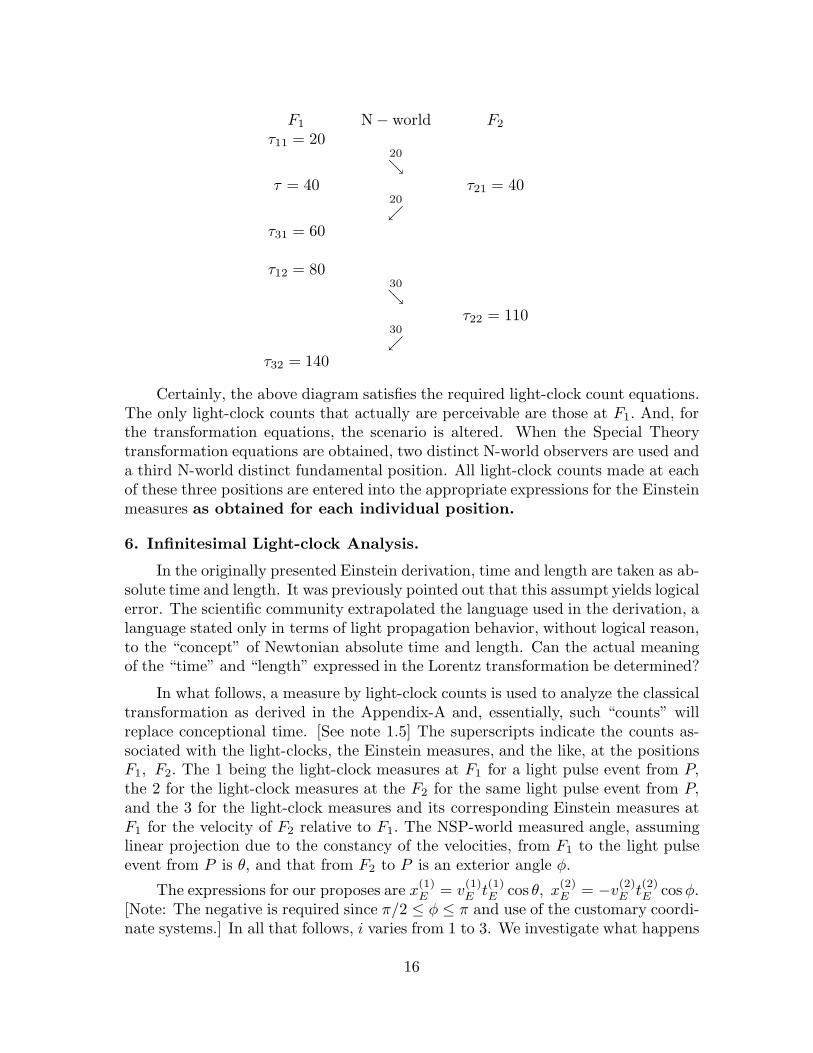
It is illustrative to show by a diagram of simple light-clock counts how thisanalysis actually demonstrates the two different modes of propagation, the NSP-world mode and the different mode when viewed from the N-world. In general, Lis always fixed and for the following analysis and, for this particular scenario, inf.light-clock c may change. This process of using N-world light-clocks to approximatethe relative velocity should only be done once due to the necessity of “indexing”the light-clocks when F1 and F2 coincide. In the following diagram, the numbersrepresent actual light-clock count numbers as perceived in the N-world. The firstcolumn are those recorded at F1, the second column those required at F2. The arrowsand the numbers above them represent our F1 comprehension of what happens whenthe transmission is considered to take place in the N-world. The Einstein measuresare only for the F1 position.

15

F1 N− world F2

τ11 = 2020

↘τ = 40 τ21 = 40

20

↙τ31 = 60

τ12 = 8030

↘τ22 = 110

30

↙τ32 = 140

Certainly, the above diagram satisfies the required light-clock count equations.The only light-clock counts that actually are perceivable are those at F1. And, forthe transformation equations, the scenario is altered. When the Special Theorytransformation equations are obtained, two distinct N-world observers are used anda third N-world distinct fundamental position. All light-clock counts made at eachof these three positions are entered into the appropriate expressions for the Einsteinmeasures as obtained for each individual position.

6. Infinitesimal Light-clock Analysis.

In the originally presented Einstein derivation, time and length are taken as ab-solute time and length. It was previously pointed out that this assumpt yields logicalerror. The scientific community extrapolated the language used in the derivation, alanguage stated only in terms of light propagation behavior, without logical reason,to the “concept” of Newtonian absolute time and length. Can the actual meaningof the “time” and “length” expressed in the Lorentz transformation be determined?

In what follows, a measure by light-clock counts is used to analyze the classicaltransformation as derived in the Appendix-A and, essentially, such “counts” willreplace conceptional time. [See note 1.5] The superscripts indicate the counts as-sociated with the light-clocks, the Einstein measures, and the like, at the positionsF1, F2. The 1 being the light-clock measures at F1 for a light pulse event from P,the 2 for the light-clock measures at the F2 for the same light pulse event from P,and the 3 for the light-clock measures and its corresponding Einstein measures atF1 for the velocity of F2 relative to F1. The NSP-world measured angle, assuminglinear projection due to the constancy of the velocities, from F1 to the light pulseevent from P is θ, and that from F2 to P is an exterior angle φ.

The expressions for our proposes are x(1)E = v

(1)E t

(1)E cos θ, x

(2)E = −v

(2)E t

(2)E cos φ.

[Note: The negative is required since π/2 ≤ φ ≤ π and use of the customary coordi-nate systems.] In all that follows, i varies from 1 to 3. We investigate what happens

16

when the standard model is now embedded back again into the non-infinitesimal

finite NSP-world. All of the “coordinate” transformation equations are in the Ap-pendix and they actually only involve ωi/c. These equations are interpreted in theNSP-world. But as far as the light-clock counts are concerned, their appropriatedifferences are only infinitely near to a standard number. The appropriate expres-sions are altered to take this into account. For simplicity in notation, it is again

assumed that “immediate” in the light-clock count process means τ(i)12 = τ

(i)31 . [See

note 3.] Consequently, t(i)1a ≈ 2uη(i), t

(i)3a ≈ 2uλ(i), η(i), λ(i) ∈ IN

+∞

. Then

t(i)Ea ≈ u(λ(i) + η(i)), λ(i), η(i) ∈ IN

+∞

. (6.1)

Now from our definition r(i)E ≈ L(λ(i) − η(i)), (λ(i) − η(i)) ∈ IN

+∞

. Hence,since all of the numbers to which st is applied are nonnegative and finite and

st(v(i)Ea) st(t

(i)Ea) = st(r

(i)Ea), it follows that

v(i)Ea ≈ L

(λ(i) − η(i))

u(λ(i) + η(i)). (6.2)

Now consider a set of two 4-tuples

(st(x(1)Ea), st(y

(1)Ea), st(z

(1)Ea), st(t

(1Ea)),

(st(x(2)Ea), st(y

(2)Ea), st(z

(2)Ea), st(t

(2)Ea)),

where they are viewed as Cartesian coordinates in the NSP-world. First, we have

st(x(1)Ea) = st(v

(1)Ea)st((t

(1)Ea)st( ∗cosθ), st(x

(2)Ea) = st(v

(2)Ea)st(t

(2)Ea)st( ∗cosφ). Now

suppose the local constancy of c. The N-world Lorentz transformation expressionsare

st(t(1)Ea) = β3(st(t

(2)Ea) + st(v

(3)Ea)st(x

(2)Ea)/c2),

st(x(1)Ea) = β3(st(x

(2)Ea) + st(v

(3)Ea)st(t

(2)Ea)),

where β3 = st((1− (v(3)Ea)2/c2)−1/2). Since L(λ(i)− η(i)) ≈ cu(λ(i)− η(i)), the finite

character of L(λ(i)−η(i)), u(λ(i)−η(i)) yields that c = st(L/u) [See note 8]. Whentransferred to the NSP-world with light-clock counts, substitution yields

t(1)Ea ≈ u(λ(1) + η(1)) ≈ β[u(λ(2) + η(2))− u(λ(2) + η(2))K(3)K(2) ∗cosφ], (6.3)

where K(i) = (λ(i) − η(i))/(λ(i) + η(i)), β = (1 − (K(3))2)−1/2.For the “distance” transformation, we have

x(1)Ea ≈ L(λ(1) − η(1)) ∗cosθ ≈

β(−L(λ(2) − η(2)) ∗cosφ +L(λ(3) − η(3))

u(λ(3) + η(3))u(λ(2) + η(2))). (6.4)

17

Assume in the NSP-world that θ ≈ π/2, φ ≈ π. Consequently, substituting into 6.4yields

−L(λ(2) − η(2)) ≈ L(λ(3) − η(3))

u(λ(3) + η(3))u(λ(2) + η(2)). (6.5)

Applying the finite property for these numbers, and, for this scenario, takinginto account the different modes of the corresponding light-clock measures, yields

L(λ(3) − η(3))

u(λ(3) + η(3))≈ −L(η(2) − λ(2))

u(λ(2) + η(2))⇒ v

(3)Ea ≈ −v

(2)Ea. (6.6)

Hence, st(v(3)Ea) = −st(v(2)

Ea). [Due to the coordinate-system selected, these aredirected velocities.] This predicts that, in the N-world, the light-clock determinedrelative velocity of F2 as measured from the F1 and F1 as measured from the F2

positions would be the same if these special infinitesimal light-clocks are used. Ifnoninfinitesimal N-world light-clocks are used, then the values will be approximatelythe same and equal in the limit.

Expression 6.4 relates the light-clock counts relative to the measure of the to-

and-fro paths of light transmission. By not substituting for x(2)Ea, it is easily seen

that x(2)Ea ≈ LG, where G is an expression written entirely in terms of various light-

clock count numbers. This implies that the so-called 4-tuples (st(x(1)Ea), st(y

(1)Ea),

st(z(1)Ea), st(t

(1Ea)), (st(x

(2)Ea),st(y

(2)Ea), st(z

(2)Ea), st(t

(2)Ea)) are not the absolute Carte-

sian type coordinates determined by Euclidean geometry and used to model Galileandynamics. These coordinates are dynamically determined by the behavior of elec-tromagnetic radiation within the N-world. Indeed, in [7], the analysis within the(outside of the monadic clusters) that leads to Prokhovnik’s conclusions is only rela-tive to electromagnetic propagation and is done by pure number Galilean dynamics.Recall that the monadic cluster analysis is also done by Galilean dynamics.

In general, when it is claimed that “length contracts” with respect to relativevelocity the “proof” is stated as follows: x′ = st(β)(x+vt); x′ = st(β)(x+vt). Thenthese two expressions are subtracted. Supposedly, this yields x′−x′ = st(β)(x−x)

since its assumed that vt = vt. For defined coordinates x(i)E , x

(i)E , i = 1, 2, a more

complete expression would be

x(1)E − x

(1)E = st(β)((x

(2)E − x

(2)E ) + (v

(3)E t

(2)E − v

(3)E t

(2)E )). (6.7)

In this particular analysis, it has been assumed that all NSP-world relativevelocities ωi, ωi ≥ 0. To obtain the classical length contraction expression, let ωi =ωi, i = 1, 2, 3. Now this implies that θ = θ, φ = φ as they appear in the velocityfigure on page 52 and that

x(1)E − x

(1)E = st(β)(x

(2)E − x

(2)E ). (6.8)

The difficulty with this expression has been its interpretation. Many moderntreatments of Special Relativity [6] argue that (6.8) has no physical meaning. But

18

in these arguments it is assumed that x(1)E − x

(1)E means “length” in the Cartesian

coordinate sense as related to Galilean dynamics. As pointed out, such a physicalmeaning is not the case. Expression (6.8) is a relationship between light-clock countsand, in general, displays properties of electromagnetic propagation within the N-world. Is there a difference between the right and left-hand sides of 6.8 when viewed

entirely from the NSP-world. First, express 6.8 as x(1)E −x

(1)E = st(β)x

(2)E −st(β)x

(2)E .

In terms of operational light-clock counts, this expression becomes

L(λ(1)

∗cos θ − η(1) ∗cos θ)− L(λ(1) ∗cos θ − η(1) ∗cos θ) ≈ (6.9)

L(λ(2)

β| ∗cos φ| − η(2)β| ∗cos φ|)− L(λ(2)β| ∗cos φ| − η(2)β| ∗cos φ|),

where finite β = (1− (K(3))2)−1/2 and | · | is used so that the Einstein velocities arenot directed numbers and the Einstein distances are comparable. Also as long asθ, φ satisfy the velocity figure on page 45, then (6.9) is independent of the specificangles chosen in the N-world since in the N-world expression (6.8) no angles appearrelating the relative velocities. That is, the velocities are not vector quantities inthe N-world, but scalars.

Assuming the nontrivial case that θ 6≈ π/2, φ 6≈ π, we have from Theorem

11.1.1 [9] that there exist Λ(i)

, N(i)

, Λ(i), N (i) ∈ IN∞, i = 1, 2 such that ∗cos θ ≈Λ

(1)/λ

(1) ≈ N(1)

/η(1) ≈ Λ(1)/λ(1) ≈ N (1)/η(1), β| ∗cos φ| ≈ Λ(2)

/λ(2) ≈ N

(2)/η(2)

≈ Λ(2)/λ(2) ≈ N (1)/η(2). Consequently, using the finite character of these quotients

and the finite character of L(λ(i)

), L(η(i)), L(λ(i)), L(η(i)), i = 1, 2, the generalthree body NSP-world view 6.9 is

L(Λ(1) −N

(1))− L(Λ(1) −N (1)) = LΓ(1) ≈

LΓ(2)1 = L(Λ

(2) −N(2)

)− L(Λ(2) −N (2)). (6.10)

The obvious interpretation of 6.10 from the simple NSP-world light propagationviewpoint is displayed by taking the standard part of expression 6.10.

st(L(Λ(1) −N

(1)))− st(L(Λ(1) −N (1))) = st(LΓ(1)) =

st(LΓ(2)1 ) = st(L(Λ

(1) −N(1)

))− st(L(Λ(1) −N (1))). (6.11)

This is the general view as to the equality of the standard NSP-world distancetraveled by a light pulse moving to-and-fro within a light-clock as used to measureat F1 and F2, as viewed from the NSPPM only, the occurrence of the light pulseevent from P . In order to interpret 6.9 for the N-world and a single NSP-worldrelative velocity, you consider additionally that ω1 = ω2 = ω3. Hence, θ = π/3 andcorrespondingly φ = 2π/3. In this case, β is unaltered and since cos π/3, cos 2π/3are nonzero and finite, 6.9 now yields

19

st(L(λ(1) − η(1)))− st(L(λ(1) − η(1))) =

st(β)(st(L(λ(2)

1 − η(2)1 ))− st(L(λ

(2)1 − η

(2)1 )))⇒

(st(Lλ(1)

)− st(Lη(1)))− (st(Lλ(1))− st(Lη(1))) =

st(β)((st(Lλ(2)

1 )− st(Lη(2)1 ))− (st(Lλ

(2)1 )− st(Lη

(2)1 ))). (6.12)

Orst(L(λ

(1) − η(1))− L(λ(1) − η(1))) =

st(L[(λ(1) − η(1))− (λ(1) − η(1))]) =

st(LΠ(1)) = st(β)st(LΠ(2)1 ) = st(βLΠ

(2)1 ) = (6.13)

st(L[(λ(1) − η(1))− (λ(1) − η(1))]) =

st(βL[(λ(2)

1 − η(2)1 )− (λ

(2)1 − η

(2)1 )]).

In order to obtain the so-called “time dilation” expressions, follow the same proce-dure as above. Notice, however, that (6.3) leads to a contradiction unless

u((λ(1)

+ η(1))− (λ(1) + η(1))) ≈ βu((λ(2)

+ η(2))− (λ(2) + η(2))). (6.14)

It is interesting, but not surprising, that this procedure yields (6.14) without hypoth-esizing a relation between the ωi, i = 1, 2, 3 and implies that the timing infinitesimallight-clocks are the fundamental constitutes for the analysis. In the NSP-world, 6.14can be re-expressed as

u((λ(1)

+ η(1))− (λ(1) + η(1))) ≈ u(λ(2)

2 − λ(2)2 ). (6.15)

Orst(u((λ

(1)+ η(1))) = st(uΠ

(1)2 ) =

st(uΠ(2)3 ) = st(u(λ

(2)

2 − λ(2)2 )). (6.16)

[See note 4.] From the N-world, the expression becomes, taking the standard partoperator,

st(u(λ(1)

+ η(1)))− st(u(λ(1) + η(1))) =

st(β)(st(u(λ(2)

+ η(2)))− st(u(λ(2) + η(2)))). (6.17)

Orst(uΠ

(1)2 ) = st(β)st(uΠ

(2)4 ) = st(βuΠ

(2)4 ) =

st(u((λ(1)

+ η(1))− (λ(1) + η(1)))) = st(βu[(λ(2)

+ η(2))− (λ(2) + η(2))]). (6.18)

20

Note that using the standard part operator in the above expressions, yields contin-uum time and space coordinates to which the calculus can now be applied. However,the time and space measurements are not to be made with respect to an universal(absolute) clock or ruler. The measurements are relative to electromagnetic prop-agation. The Einstein time and length are not the NSPPM time and length, butrather they are concepts that incorporate a mode of measurement into electromag-netic field theory. This mode of measurement follows from the one wave propertyused for Special Theory scenarios, the property that, in the N-world, the propaga-tion of a photon do not take on the velocity of its source. It is this that helps clarifyproperties of the NSPPM. Expressions such as (6.13), (6.18) will be interpreted inthe next sections of this paper.

7. An Interpretation.

In each of the expressions (6.i), i = 10, . . . , 18 the infinitesimal numbers L, uare unaltered. If this is the case, then the light-clock counts would appear to bealtered. As shown in Note [2], alteration of c can be represented as alterationsthat yield infinite counts. Thus, in one case, you have a specific infinitesimal Land for the other infinitesimal light-clocks a different light-clock c is used. But,L/u = c. Consequently the only alteration that takes place in N-world expressions(6.i), i = 12, 13, 17, 18 is the infiniteimal light-clocks that need to be employed. Thisis exactly what (6.13) and (6.18) state if you consider it written as say, (βL) · ratherthan L(β ·). Although these are external expressions and cannot be “formally”transferred back to the N-world, the methods of infinitesimal modeling require theconcepts of “constant” and “not constant” to be preserved.

These N-world expressions can be re-described in terms of N-world approxi-mations. Simply substitute

.= for =, a nonzero real d [resp. µ] for L [resp. u] and

real natural numbers for each light-clock count in equations (6.i), i = 12, 17. Thenfor a particular d [resp. µ] any change in the light-clock measured relative velocityvE would dictate a change in the the light-clocks used. Hence, the N-world neednot be concerned with the idea that “length” contracts but rather it is the requiredlight-clocks change. It is the required change in infiniteimal light-clocks that leadto real physical changes in behavior as such behavior is compared to a standardbehavior. But, in many cases, the use of light-clocks is not intended to be a literal

use of such instruments. For certain scenarios, light-clocks are to be consideredas analog models that incorporate electromagnetic energy properties. [See note 18,first paragraph.]

The analysis given in the section 3 is done to discover a general property forthe transmission of electromagnetic radiation. It is clear that property (*) doesnot require that the measured velocity of light be a universal constant. All that isneeded is that for the two NSP-world times ta, tb that st(`(ta)) = st(`1(tb)). Thismeans that all that is required for the most basic aspects of the Special Theory tohold is that at two NSP-world times in the F1 → F2, F2 → F1 reflection processst(`(ta)) = st(`1(tb)), ta a time during the transmission prior to reflection andtb after reflection. If `, `1 are nonstandard extensions of standard functions v, v1

21

continuous on [a, b], then given any ε ∈ IR+ there is a δ such that for each t, t′ ∈ [a, b]

such that |t − t′| < δ it follows that |v(t)− v(t′)| < ε/3 and |v1(t) − v1(t′)| < ε/3.

Letting t3 − t1 < δ, then |ta − tb| < δ. Since ∗v(ta) = `(ta) ≈ ∗v1(tb) = `1(tb), *-transfer implies | ∗v(t2)− ∗v1(t2)| < ε. [ See note 5.] Since t2 is a standard number,|v(t2)−v1(t2)| < ε implies that v(t2) = v1(t2). Hence, in this case, the two functions`, `1 do not differentiate between the velocity c at t2. But t2 can be considered anarbitrary (i.e. NSPPM) time such that t1 < t2 < t3. This does not require c tobe the same for all cosmic times only that v(t) = v1(t), t1 < t < t3.

The restriction that `, `1 are extended standard functions appears necessary for

our derivation. Also, this analysis is not related to what ` may be for a stationarylaboratory. In the case of stationary F1, F2, then the integrals are zero in equation(19) of section 3. The easiest thing to do is to simply postulate that st( ∗v(ta)) isa universal constant. This does not make such an assumption correct.

One of the properties that will allow the Einstein velocity transformation ex-pression to be derived is the equilinear property. This property is weaker thanthe c = constant property for light propagation. Suppose that you havewithin the NSP-world three observers F1, F2, F3 that are linearly related. Further,suppose that w1 is the NSP-world velocity of F2 relative to F1 and w2 is the NSP-world velocity of F3 relative to F2. It is assumed that for this nonmonadic clustersituation, that Galilean dynamics also apply and that st(w1) + st(w2) = st(w3).Using the description for light propagation as given in section 3, let t1 be the cosmictime when a light pulse leaves F1, t2 when it “passes” F2, and t3 the cosmic timewhen it arrives at F3.

From equation (3.15), it follows that

st(w1) = st( ∗v1(t1a))st

(

∗

∫ t2

t1

1

xdx

)

+

[st(w2) =]st( ∗v2(t2a))st

(

∗

∫ t3

t2

1

xdx

)

=

st(w3) = st( ∗v3(t3a))st

(

∗

∫ t3

t1

1

xdx

)

. (7.1)

If st( ∗v1(t1a)) = st( ∗v2(t2a)) = st( ∗v3(t3a)), then we say that the velocityfunctions ∗v1,

∗v2,∗v3 are equilinear. The constancy of c implies equilinear, but

not conversely. In either case, functions such as ∗v1 and ∗v2 need not be the samewithin a stationary laboratory after interaction.

Experimentation indicates that electromagnetic propagation does “appear” tobehave in the N-world in such a way that it does not accquire the velocity ofthe source. The light-clock analysis is consistent with the following speculation.Depending upon the scenario, the uniform velocity yields an effect viainteractions with the subparticle field (the NSPPM) that uses a photonparticle behavioral model. This is termed the (emis) effect. Recall that

22

a “light-clock” can be considered as an analog model for the most basic of theelectromagnetic properties. On the other hand, only those experimental methodsthat replicate or are equivalent to the methods of Einstein measure would be relativeto the Special Theory. This is one of the basic logical errors in theory application.The experimental language must be related to the language of the derivation. Theconcept of the light-clock, linear paths and the like are all intended to imply NSPPMinteractions. Any explanation for experimentally verified Special Theory effectsshould be stated in such a language and none other. I also point out that thereare no paradoxes in this derivation for you cannot simply “change your mind” withrespect to the NSPPM. For example, an observer is either in motion or not inmotion, and not both with respect to the NSPPM.

8. A Speculation and Ambiguous Interpretations

Suppose that the correct principles of infinitesimal modeling were known priorto the M-M (i.e. Michelson-Morley) experiment. Scientists would know that the(mathematical) NSPPM is not an N-world entity. They would know that they couldhave very little knowledge as to the refined workings of this NSP-world NSPPMsince ≈ is not an = . They would have been forced to accept the statement of MaxPlanck that “Nature does not allow herself to be exhaustively expressed in humanthought.”[The Mechanics of Deformable Bodies, Vol. II, Introduction to Theoretical

Physics, Macmillian, N.Y. (1932),p. 2.]

Further suppose, that human comprehension was advanced enough so that allscientific experimentation always included a theory of measurement. The M-Mexperiment would then have been performed to learn, if possible, more about thisNSP-world NSPPM. When a null finding was obtained then a derivation such asthat in section 3 might have been forthcoming. Then the following two expressionswould have emerged from the derivation.

The Einstein method for measurement - the “radar” method - is used (seeA3, p. 52) to determining the relative velocity of the moving light-clock. UsingAppendix-A equations (A14), let P correspond to F2. Then θ = 0, φ = π/2. Since,x(2) = 0 from page 54, then F2 is the s-point Hence, t2E = t(2). The superscript andsubscript s represents local measurements about the s-point, using various devices,for laboratory standards (i.e. standard behavior) and using infinitesimal light-clocksor approximating devices such as atomic-clocks. [Due to their construction atomicclocks are effected by relativistic motion and gravitational fields approximately asthe infinitesimal light-clock’s counts are effected.] Superscript or subscript m indi-cates local measurements, using the same devices, for an entity considered at them-point in motion relative to the s-point, where Einstein time and distance via theradar method as registered at s are used to investigate m-point behavior. For ex-ample, m-point time is measured at the s-point via infinitesimal light clock and theradar method and this represents time at the m-point. To determine how physicalbehavior is being altered, the m and s-measurements are compared. Many claimthat you can replace each s with m, and m with s in what follows. This may lead

23

to various controversies which are elimianted in part 3. A specific interpretation of

st(β)−1(t(s) − t(s)) = t

(m)E − t

(m)E (8.1)

or the corresponding

st(β)−1(x(s) − x(s)) = x(m)E − x

(m)E (8.2)

seems necessary. However, (8.2) is unnecessary since vE(st(β)−1(t(s) − t(s))) =

vE(t(m)E − t

(m)E ) yields (8.2), which can be used when convienient. Thus, only the in-

finitesimal light-clock “time” alterations are significant. Actual length as measuredvia the radar method is not altered. It is the clock counts that are altered.

If, in (8.2), which is employed for convenience, x(s) − x(s) = Us (note thatx(s) = vEt(s) etc.) is interpreted as “any” standard unit for length measurement at

the s-point and x(m)E −x

(m)E ) = Um the same “standard” unit for length measurement

in a system moving with respect to the NSPPM (without regard to direction), thenfor equality to take place the unit of measure Um may seem to be altered in themoving system. Of course, it would have been immediately realized that the errorin this last statement is that Us is “any” unit of measure. Once again, the error inthese two statements is the term “any.” (This problem is removed by applicationof (14)a or (14)b p. 60.)

If, in (8.2), which is employed for convenience, x(s) − x(s) = Us (Note thatx(s) = vEt(s).) is interpreted as “any” standard unit for length measurement at the

s-point and x(m)E − x

(m)E ) = Um the same “standard” unit for length measurement

in a system moving with respect to the NSPPM (without regard to direction), thenfor equality to take place the unit of measure Um may seem to be altered in themoving system. Of course, it would have been immediately realized that the errorin this last statement is that Us is “any” unit of measure. Once again, the error inthese two statements is the term “any.” (This problem is removed by applicationof (14)a or (14)b p. 60.)

Consider experiements such as the M-M, Kennedy-Thorndike and many oth-ers. When viewed from the wave state, the interferometer measurement tech-nique is determined completely by a light-clock type process – the number oflight waves in the linear path. We need to use Lm

sc, a scenario associated lightunit, for Um and use a Ls

sc for Us. It appears for this particular scenario, thatLs

sc may be considered the private unit of length in the NSP-world, such as L,used to measure NSP-world light-path length. The “wavelength” λ of any lightsource must also be measured in the same light units. Let λ = NsLs

sc. Takinginto consideration a unit conversion factor k between the unknown NSP-world pri-vate units, such that st(kLs

sc) = Us, the number of light waves in s-laboratorywould be As

st(kLssc)/N

sst(kLs

sc) = As/Ns, where As is a pure number suchthat As

st(kLssc) is the “path-length” using the units in the s-system. In the

moving system, assuming that this simple aspect of light propagation holds in

24

the NSP-world and the N-world which we did to obtain the derivation in sec-tion 3, it is claimed that substitution yields st(β−1AskLs

sc)/st(β−1NskLs

sc) =As

st(β−1kLssc)/N

sst(β−1kLs

sc) = As/Ns. Thus there would be no difference inthe number of light waves in any case where the experimental set up involved thesum of light paths each of which corresponds to the to-and-fro process [1: 24].Further, the same conclusions would be reached using (8.2). not relevant to aSagnac type of experiment. However, this does not mean that a similar derivationinvolving a polygonal propagation path cannot be obtained. [Indeed, this may bea consequence of a result to be derived in article 3. However, see note 8 part 4, p.80.]

Where is the logical error in the above argument? The error is the object uponwhich the st(β)−1 operates. Specifically (6.13) states that

st(β)−1(AskLssc)

(emis)←→ β−1(LΠ(s)) = (β−1L)Π(s) and (8.3)

st(β)−1(NskLssc)

(emis)←→ β−1(LΠ(s)1 ) = (β−1L)Π

(s)1 . (8.4)

It is now rather obvious that the two (emis) aspects of the M-M experiment nullifyeach other. Also for no finite w can β ≈ 0. There is a great difference betweenthe propagation properties in the NSP-world and the N-world. For example, theclassical Doppler effect is an N-world effect relative to linear propagation. Ratherthan indicating that the NSPPM is not present, the M-M results indicateindirectly that the NSP-world NSPPM exists.

Apparently, the well-known Ives-Stillwell, and all similar, experiments used inan attempt to verify such things as the relativistic redshift are of such a naturethat they eliminate other effects that motion is assumed to have upon the scenarioassociated electromagnetic propagation. What was shown is that the frequencyν of the canal rays vary with respect to a representation for vE measured fromelectromagnetic theory in the form νm = st(β)−1νs. First, we must investigate whatthe so-called time dilation statement (8.2) means. What it means is exemplified by(6.14) and how the human mind comprehends the measure of “time.” In the scenarioassociated (8.2) expression, for the right and left-sides to be comprehensible, theexpression should be conceived of as a measure that originates with infinitesimallight-clock behavior. It is the experience with a specific unit and the number ofthem that “passes” that yields the intuitive concept of “observer time.” On theother hand, for some purposes or as some authors assume, (8.2) might be viewedas a change in a time unit T s rather than in an infinitesimal light-clock. Both ofthese interpretations can be incorporated into a frequency statement. First, relativeto the frequency of light-clock counts, for a fixed stationary unit of time T s, (8.2)reads

st(β)−1Cssc/T s .

= Cmsc/T s ⇒ st(β)−1Cs

sc.= Cm

sc . (8.5)

But according to (6.18), the Cssc and Cm

sc correspond to infinitesimal light-clocksmeasures and nothing more than that. Indeed, (8.5) has nothing to do with the

25

concept of absolute “time” only with the different infinitesimal light-clocks thatneed to be used due to relative motion. This requirement may be due to (emis).Indeed, the “length contraction” expression (8.1) and the “time dilation” expression(8.2) have nothing to do with either absolute length or absolute time. These twoexpressions are both saying the same thing from two different viewpoints. There isan alteration due to the (emis). [Note that the second

.= in (8.5) depends upon the

T s chosen.]On the other hand, for a relativistic redshift type experiment, the usual inter-

pretation is that νs.= p/T s and νm

.= p/Tm. This leads to p/Tm .

= st(β)−1p/T s ⇒Tm .

= st(β)T s. Assuming that all frequency alterations due to (emis) have beeneliminated then this is interpreted to mean that “time” is slower in the movingexcited hydrogen atom than in the “stationary” laboratory. When compared to(8.5), there is the ambiguous interpretation in that the p is considered the same forboth sides (i.e. the concept of the frequency is not altered by NSPPM motion). Itis consistent with all that has come before that the Ives-Stillwell result be writtenas νs

.= p/T s and that νm

.= q/T s, where “time” as a general notion is not altered.

This leads to the expression

st(β)−1p.= q [= in the limit]. (8.6)

Expression (8.6) does not correspond to a concept of “time” but rather to theconcept of alterations in emitted frequency due to (emis). One, therefore, has anambiguous interpretation that in an Ives-Stillwell scenario the number that repre-sents the frequency of light emitted from an atomic unit moving with velocity ω withrespect to the NSPPM is altered due to (emis). This (emis) alteration depends uponK(3). It is critical that the two different infinitesimal light-clock interpretations beunderstood. One interpretation is relative to electromagnetic propagation theory.In this case, the light-clock concept is taken in its most literal form. The secondinterpretation is relative to an infinitesimal light-clock as an analogue model. Thismeans that the cause need not be related to propagation but is more probably dueto how individual constituents interact with the NSPPM. The exact nature of thisinteraction and a non-ambiguous approach needs further investigation based uponconstituent models since the analogue model specifically denies that there is sometype of absolute time dilation but, rather, signifies the existences of other possiblecauses. [In article 3, the νm = st(β)−1νs is formally and non-ambiguously derivedfrom a special line-element, a universal functional requirement and Schrodinger’sequation.]

It is clear, however, that under our assumption that the scalar velocities in theNSP-world are additive with respect to linear motion, then if F1 has a velocity ωwith respect to the NSPPM and F2 has the velocity ω′, then it follows that thelight-clock counts for F1 require the use of a different light-clock with respect toa stationary F0 due to the (emis) and the light-clocks for F2 have been similarlychanged with respect to a stationary F0 due to (emis). Consequently, a light-clockrelated expressed by K(3) is the result of the combination, so to speak, of these

26

two (emis) influences. The relative NSPPM velocity ω2 of F1 with respect to F2

which yields the difference between these influences is that which would satisfiesthe additive rule for three linear positions.

As previously stated, within the NSP-world relative to electromagnetic propa-gation, observer scalar velocities are either additive or related as discussed above.Within the N-world, this last statement need not be so. Velocities of individualentities are modeled by either vectors or, at the least, by signed numbers. Once theN-world expression is developed, then it can be modified in accordance with theusual (emis) alterations, in which case the velocity statements are N-world Einsteinmeasures. For example, deriving the so-called relativistic Dopplertarian effect, thecombination of the classical and the relativistic redshift, by means of a NSPPMargument such as appears in [7] where it is assumed that the light propagation lawswith respect to the photon concept in the NSP-world are the same as those in theN-world, is in logical error. Deriving the classical Doppler effect expression then,when physically justified, making the wave number alteration in accordance withthe (emis) would be the correct logic needed to obtain the relativistic Dopplertarianeffect. [See note 6.]

Although I will not, as yet, re-interpreted Special Relativity results with respectto this purely electromagnetic interpretation, it is interesting to note the followingtwo re-interpretations. The so-called variation of “mass” was, in truth, originallyderived for imponderable matter (i.e. elementary matter.) This would lead oneto believe that the so-called rest mass and its alteration, if experimentally verified,is really a manifestation of the electromagnetic nature of such elementary matter.Once again the so-called mass alteration can be associated with an (emis) concept.The µ-meson decay rate may also show the same type of alteration as appearsto be the case in an Ives-Stillwell experiment. It does not take a great stretchof the imagination to again attribute the apparent alteration in this rate to an(emis) process. This would lead to the possibility that such decay is controlled byelectromagnetic properties. Indeed, in order to conserve various things, µ-mesondecay is said to lead to the generation of the neutrino and antineutrino. [After thispaper was completed, a method was discovered that establishes that predicted massand decay time alterations are (emis) effects. The derivations are found in article3.]

I note that such things as neutrinos and antineutrinos need not exist. Indeed,the nonconservation of certain quantities for such a scenario leads to the conclusionthat subparticles exist within the NSP-world and carry off the “missing” quanti-ties. Thus the invention of such objects may definitely be considered as only abookkeeping technique.

As pointed out, all such experimental verification of the properly interpretedtransformation equations can be considered as indirect evidence that the NSP-world NSPPM exists. But none of these results should be extended beyond theexperimental scenarios concerned. Furthermore, I conjecture that no matter howthe human mind attempts to explain the (emis) in terms of a human language, it willalways be necessary to postulate some interaction process with the NSPPM without

27

being able to specifically describe this interaction in terms of more fundamentalconcepts. Finally, the MA-model specifically states that the Special Theory is alocal theory and should not be extended, without careful consideration, beyond alocal time interval [a, b].

9. Reciprocal Relations

As is common to many mathematical models, not all relations generated by themathematics need to correspond to physical reality. This is the modern approach tothe length contradiction controversy [6]. Since this is a mathematical model, thereis a theory of correspondence between the physical language and the mathematicalstructure. This correspondence should be retained throughout any derivation. Thisis a NSPPM theory and what is stationary or what is not stationary with respectto the NSPPM must be maintained throughout any correspondence. This appliesto such reciprocal relations as

st(β)−1(t(m)E − t

(m)E ) = t

(s) − t(s) (9.1)

andst(β)−1(x

(m)E − x

(m)E ) = x(s) − x(s) (9.2)

Statement (8.1) and (9.1) [resp. (8.2) and (9.2)] both hold from the NSPPM view-point only when vE = 0 since it is not the question of the N-world viewpoint ofrelative velocity but rather the viewpoint that F1 is fixed and F2 is not fixed in theNSPPM or ω ≤ ω′. The physical concept of the (s) and (m) must be maintainedthroughout the physical correspondence. Which expression would hold for a partic-ular scenario depends upon laboratory confirmation. This is a scenario associatedtheory. All of the laboratory scenarios discussed in this paper use infinitesimalized(9.1) and (9.2) as derived from line-elements and the “view” or comparison is alwaysmade relative to the (s). Other authors, such as Dingle [1] and Builder [7], have, ina absolute sense, excepted one of these sets of equations, without derivation, ratherthe other set. I have not taken this stance in this paper.

One of the basic controversies associated with the Special Theory is whether(8.2) or (8.1) [resp. (9.1) or (9.2)] actually have physical meaning. The notion isthat either “length” is a fundamental concept and “time” is defined in terms of it,or “time” is a fundamental concept and length is defined in terms of it. Ives, andmany others assumed that the fundamental notion is length contraction and nottime dilation. The modern approach is the opposite of this. Length contractionin the N-world has no physical meaning, but time dilation does [6]. We know thattime is often defined in terms of length and velocities. But, the length or time beingconsidered here is Einstein length or Einstein time. This is never mentioned whenthis problem is being considered. As discussed at the end of section 3, Einsteinlength is actually defined in terms of infinitesimal light-clocks or in terms of theEinstein velocity and Einstein time. As shown after equation (8.2) is considered, itis only infinitesimal light-clock “time” that is altered and length altertions is buta technical artefact. The changes in the infinitesimal light-clock counts yields an

28

analogue model for physical changes that cause Special Theory effects. [See note7.]

{Remark: Karl Popper notwithstanding, it is not the sole purpose of mathemat-ical models to predict natural system behavior. The major purpose is to maintainlogical rigor and, hopefully, when applicable to discover new properties for natu-ral systems. I have used in this speculation a correspondence theory that takesthe stance that any verifiable Special Theory effect is electromagnetic in charac-ter rather than a problem in measure. However, whether such effects are simplyeffects relative to the propagation of electromagnetic information or whether theyare effects relative to the constituents involved cannot be directly obtain from theSpecial Theory. All mathematically stated effects involve the Einstein measure ofrelative velocity, vE – a propagation related measure. The measure of an effectshould also be done in accordance with electromagnetic theory. As demonstrated,the Special Theory should not be unnecessarily applied to the behavior of all na-ture systems since it is related to electromagnetic interaction; unless, of course, allnatural systems are electromagnetic in character. Without strong justification, theassumption that one theory does apply to all scenarios is one of the greatest errorsin mathematically modeling. But, if laboratory experiments verify that alterationsare taking place in measured quantities and these variations are approximated inaccordance with the Special Theory, then this would indicate that either the al-terations are related to electromagnetic propagation properties or the constituentshave an appropriate electromagnetic character.}

NOTES

[1] (a) Equation (3.9) is obtained as follows: since t ∈ [a, b], t finite and notinfinitesimal. Thus division by t preserves ≈ . Hence,

[

t

(

∗s(t + dt)− s(t)

dt

)

− s(t)

]

/t2 ≈ `(t)

t. (1)

Since t is an arbitrary standard number and dt is assume to be an arbitrary and ap-propriate nonzero infinitesimal and the function s(t)/t is differentiable, the standardpart of the left-side equals the standard part of the right-side. [For the end-points,the left and right derivatives are used.] Thus

d(s(t)/t)

dt=

v(t)

t, (2)

for each t ∈ [a, b]. By *-transfer, equation (3.9) holds for each t ∈ ∗ [a, b].(b) Equation (3.10) is then obtained by use of the *-integral and the funda-

mental theorem of integral calculus *-transferred to the NSP-world. It is useful toview the definite integral over a standard interval say [t1, t] as an operator, at least,defined on the set C([t1, t], IR) of all continuous real valued functions defined on[t1, t]. Thus, in general, the fundamental theorem of integral calculus can be viewed

29

as the statement that (f ′, f(t) − f(t1)) ∈∫ t

t1. Hence ∗(f ′, f(t)− f(t1)) ∈ ∗

∫ t

t1⇒

( ∗f ′, ∗(f(t) − f(t1))) ∈ ∗∫ t

t1⇒ ( ∗f ′, f(t) − f(t1)) ∈ ∗

∫ t

t1.

(c) To obtain the expressions in (3.19), consider f(x) = 1/x. Then ∗f is limited

and S-continuous on ∗ [a, b]. Hence ( ∗f, ln t2 − ln t1) ∈ ∗∫ t2

t1. Hence st(( ∗f, ln t2 −

ln t1)) = (f, ln t2 − ln t1) ∈∫ t2t1

. Further (3.19) can be interpreted as an interactionproperty.

[1.5] Infinitesimal light-clocks are based upon the QED model as to how elec-trons are kept in a range of distances in a hydrogen atom proton. The back-and-forth exchanges of photons between a proton and electron replaces “reflection” andthe average distance between the proton and electron is infinitesimalized to the L.In this case, the proton and electron are also infinitesimalized. The large numberof such interchanges over a second, in the model, is motivation for the use of themembers of IN+

∞as count numbers.

[2] The basic theorem that allows for the entire concept of infinitesimal light-clocks and the analysis that appears in this monograph has not been stated. Astaken from “The Theory of Ultralogics,”the theorem, for this application, is:

Theorem 11.1.1 Let 10ω ∈ IN∞. Then for each r ∈ IR there exists an x ∈{2m/10ω | (2m ∈ ∗Z) ∧ (|2m| < λ10ω)}, for any λ ∈ IN∞, such that x ≈ r (i.e.x ∈ µ(r).)

Theorem 11.1.1 holds for other members of IN∞. Let L = 1/10ω where ω isany hyperreal infinite natural number (i.e. ω ∈ IN∞). Hence, by this theorem, forany positive real number r there exists some m ∈ IN∞ such that 2st(m/10ω) = r.I point out that for this nonzero case it is necessary that m ∈ IN∞ for if m ∈ IN,then st(m/10ω) = 0. Since c = st(L/u), then 2st(um) = 2st((L/c)m) = t = r/cas required. Thus, the infinitesimal light-clock determined length r and intervalof time t are determined by the difference in infinitesimal light-clock counts 2m =(λ − η). Note that our approach allows the calculus to model this behavior bysimply assuming that the standard functions are differentiable etc.

[2.5] (4 JUN 2000) Equating these counts here and elsewhere is done so thatthe “light pulse” is considered to have a “single instantaneous effect” from a globalviewpoint and as such is not a signal in that globally it contains no information.Thus additional analysis is needed before one can state that the Special Theoryapplies to informational transmissions. It’s obvious from section 7 that the actualvalue for c may depend upon the physical application of this theory.

[3] At this point and on, the subscripts on the τ have a different meaning thanpreviously indicated. The subscripts denote process numbers while the superscriptdenotes the position numbers. For example, τ 2

12 means the light-clock count numberwhen the second light pulse leaves F2 and τ 2

31 would mean the light-clock countnumber when the first light pulse returns to position F2.

The additional piece of each subscript denoted by the a on this and the fol-lowing pages indicates, what I thought was obvious from the lines that follow their

30

introduction, that these are approximating numbers that are infinitesimally near tostandard NSP-world number obtained by taking the standard part.

[4] Note that such infinite hyperreal numbers as Π(2)3 (here and elsewhere)

denote the difference between two infinitesimal light-clock counts and since we areexcluding the finite number infinitesimally near to 0, these numbers must be infinitehyperreal. Infinitesimal light-clocks can be assumed to measure this number by useof a differential counter. BUT it is always to be conceived of as an infinitesimallight-clock “interval” (increment, difference, etc.) It is important to recall this whenthe various line-elements in the next article are considered.

[5] This result is obtained as follows: since ta ≤ t2 ≤ tb, it follows that |ta−t2| <δ, |tb− t2| < δ. Hence by *-transfer, | ∗v(t2)− ∗v(ta)| < ε/3, | ∗v1(tb)− ∗v1(t2)| <ε/3. Since we assume arbitrary ε/3 is a standard positive number, then ∗v(ta) =`(ta) ≈ ∗v1(tb) = `1(tb)⇒ | ∗v(ta)− ∗v1(tb)| < ε/3. Hence | ∗v(t2)− ∗v1(t2)| < ε.

[6] In this article, I mention that all previous derivations for the completeDopplertarian effect (the N-world and the transverse) are in logical error. Althoughthere are various reasons for a redshift not just the Dopplertarian, the electromag-netic redshift based solely upon properties of the NSPPM can be derived as follows:

(i) let νs denote the “standard” laboratory frequency for radiation emittedfrom an atomic system. This is usually determined by the observer. The NSP-world alteration in emitted frequency at an atomic structure due to (emis) is γνs =νradiation, where γ =

√

1− v2E/c2 and vE is the Einstein measure of the relative

velocity using light-clocks only.

(ii) Assuming that an observer is observing this emitted radiation in a di-rect line with the propagation and the atomic structure is receding with veloc-ity v from the observer, the frequency of the electromagnetic propagation, withinthe N-world, is altered compared to the observers standards. This alteration isνradiation(1/(1 + v/c)) = νreceived. Consequently, this yields the total alteration asγνs(1/(1 + v/c)) = νreceived. Note that v is measured in the N-world and can beconsidered a directed velocity. Usually, if due to the fact that we are dealing withelectromagnetic radiation, we consider v the Einstein measure of linear velocity (i.e.v = vE), then the total Dopplertarian effect for v ≥ 0 can be written as

νs

(

1− vE/c

1 + vE/c

)1/2

= νreceived. (3)

It should always be remembered that there are other reasons, such as the grav-itational redshift and others yet to be analyzed, that can mask this total Doppler-tarian redshift.

[7] A question that has been asked relative to the new derivation that yieldsSpecial Theory resilts is why in the N-world do we have the apparent nonballisticeffects associated with electromagnetic radiation? In the derivation, the oppositewas assumed for the NSP-world monadic clusters. The constancy of the measure,by light-clocks and the like, of the F1 → F2, F2 → F1 velocity of electromagnetic

31

radiation was modeled by letting st(ta) = st(tb). As mentioned in the section onthe Special Theory, the Einstein velocity measure transformation expression canbe obtained prior to embedding the world into a hyperbolic velocity space. It isobtained by considering three in-line standard positions F1, F2, F3 that have theNSP-world velocities w1 for F2 relative to F1, w2 for F3 relative to F2 and the simplecomposition w3 = w1 + w2 for F3 relative to F1. Then simple substitution in thisexpression yields

v(3)E = (v

(1)E + v

(2)E )/

(

1 +v(1)E v

(2)E

c2

)

. (4)

This relation is telling us something about the required behavior in the N-worldof electromagnetic radiation. To see that within the N-world we need to assume

for electromagnetic radiation effects the nonballistic property, simply let v(2)E = c

or v(2)E

.= c. Then v

(3)E = c, or

.= c. Of course, the reason we do not have a con-

tradiction is that we have two distinctly different views of the behavior of electro-magnetic radiation, the NSP-world view and the N-world view. Further, note how,for consistency, the velocity of electromagnetic radiation is to be measured. It ismeasured by the Einstein method, or equivalent, relative to a to-and-fro path andmeasures of “time” and “distance” by means of a (infinitesimal) light-clock counts.Since one has the NSPPM, then letting F1 be fixed in that medium, assuming that“absolute” physical standards are measured at F1, equation (4) indicates why, incomparison, physical behavior varies at F2 and F3. The hyperbolic velocity spaceproperties are the cause for such behavior differences.

I am convinced that the dual character of the Special theory derivation requiresindividual reflection in order to be understood fully. In the NSP-world, electromag-netic radiation behaves in one respect, at least, like a particle in that it satisfies theballistic nature of particle motion. The reason that equation (3) is derivable is dueto the definition of Einstein time. But Einstein time, as measured by electromag-

netic pulses, models the nonballistic or one and only one wave-like property in that

a wave front does not partake of the velocity of the source. This is the reason why Iwrote that a NSPPM disturbance would trace the same operational linear light-clock

distance. The measuring light-clocks are in the N-world in this case. F1 is modeledas fixed in the NSPPM and F2 has an NSP-world relative velocity. The instant thelight pulse is reflected back to F1 it does not, from the N-world viewpoint, partakeof the N-world relative velocity and therefore traces out the exact same apparentN-world linear path. The position F2 acts like a virtual position having no otherN-world effect upon the light pulse except a reversal of direction.

[8] This expression implies that the “c” that appears here and elsewhere is tobe measured by infinitesimal light-clocks. As noted u ≈ L/c, but infinitesimal light-clock construction yields that u = L/c. For a fixed L, from the NSPPM viewpoint,u is fixed. Notice that t(i) ≈ u(2η(i)) = u(γ(i)), γ(i) ∈ IN

+∞

.

[9] In both parts of this monograph, conceptual time is used and NSPPM andgravitational field processes yield non-classical relations between these times. For

32

example, t2 =√

t1t3. For the Special Theory, there is only one aspect of physical-world behavior that corresponds to the infinitesimal-world behavior. This is the sud-den photon interaction with other particles. Hence, such interactions are particle-like, which predicts the QED assumption. An NSPPM velocity for the source isalways necessary for photon emission due to a photon’s momentum. In the actualderivation, the wave-property, where classical wave-mechanics can be applied, isnot a property within the infinitesimal-world. Classical wave-mechanics model pho-ton paths of motion within our physical-world. Wave-behavior emerges after the”st” operator is applied. The particle behavior takes place only for the interactions.Hence, the probability interpretation that comes from a photon’s wave-property canbe used to predict the number of photon interactions. Consequently, there is neithera contradiction between these two interpretations nor the particle assumption.

[10] Modern derivations attempt to remove the mode of measurement, but byso doing the twin anomaly occurs that cannot by removed even by using GR [7]. Itcan be removed by using the method presented here and Einstein measures.

REFERENCES

1 Dingle, H., The Special Theory of Relativity, Methuen’s Monographs on PhysicalSubjects, Methuen & Co. LTD, London, 1950.

2 Herrmann, R. A., Some Applications of Nonstandard Analysis to Undergrad-

uate Mathematics – Infinitesimal Modeling, Instructional Development Project,Mathematics Dept. U. S. Naval Academy, Annapolis, MD 21402-5002, 1991.http://arxiv.org/abs/math/0312432

3 Herrmann, R. A., Fractals and ultrasmooth microeffects. J. Math. Physics.,30(1989), 805–808.

4 Herrmann, R. A., Physics is legislated by a cosmogony. Speculat. Sci. Technol.,11(1988), 17–24.

5 Herrmann, R. A., Rigorous infinitesimal modelling, Math. Japonica 26(4)(1981),461–465.

6 Lawden, D. F., An Introduction to Tensor Calculus, Relativity and Cosmology,John Wiley & Son, New York, 1982.

7 Prokhovnik, S. J., The Logic of Special Relativity, Cambridge University Press,Cambridge, 1967.

8 Stroyan, K. D. and Luxemburg, W. A. J. 1976. Introduction to the Theory of

Infinitesimals, Academic Press, New York.

9 Herrmann, R. A., The Theory of Ultralogics, (1992)http://www.arxiv.org/abs/math.GM/9903081http://www.arxiv.org/abs/math.GM/9903082

10 Davis M., Applied Nonstandard Analysis, John Wiley & Sons, New York, 1977.

NOTE: Since 1994, major portions of this monograph have been published in variousjournals.

33

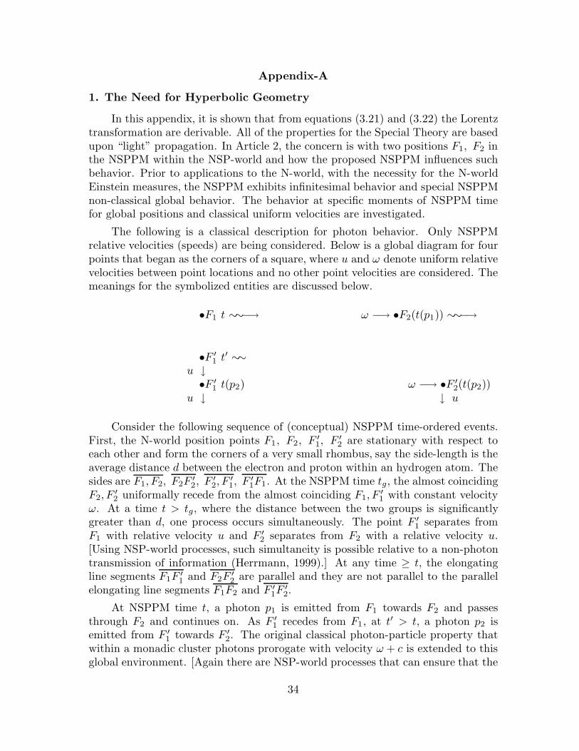
Appendix-A

1. The Need for Hyperbolic Geometry

In this appendix, it is shown that from equations (3.21) and (3.22) the Lorentztransformation are derivable. All of the properties for the Special Theory are basedupon “light” propagation. In Article 2, the concern is with two positions F1, F2 inthe NSPPM within the NSP-world and how the proposed NSPPM influences suchbehavior. Prior to applications to the N-world, with the necessity for the N-worldEinstein measures, the NSPPM exhibits infinitesimal behavior and special NSPPMnon-classical global behavior. The behavior at specific moments of NSPPM timefor global positions and classical uniform velocities are investigated.

The following is a classical description for photon behavior. Only NSPPMrelative velocities (speeds) are being considered. Below is a global diagram for fourpoints that began as the corners of a square, where u and ω denote uniform relativevelocities between point locations and no other point velocities are considered. Themeanings for the symbolized entities are discussed below.

•F1 t ∼∼−→ ω −→ •F2(t(p1)) ∼∼−→

•F ′

1 t′ ∼∼u ↓•F ′

1 t(p2) ω −→ •F ′

2(t(p2))u ↓ ↓ u

Consider the following sequence of (conceptual) NSPPM time-ordered events.First, the N-world position points F1, F2, F ′

1, F ′

2 are stationary with respect toeach other and form the corners of a very small rhombus, say the side-length is theaverage distance d between the electron and proton within an hydrogen atom. Thesides are F1, F2, F2F ′

2, F ′

2, F′

1, F ′

1F1. At the NSPPM time tg, the almost coincidingF2, F

′

2 uniformally recede from the almost coinciding F1, F′

1 with constant velocityω. At a time t > tg, where the distance between the two groups is significantlygreater than d, one process occurs simultaneously. The point F ′

1 separates fromF1 with relative velocity u and F ′

2 separates from F2 with a relative velocity u.[Using NSP-world processes, such simultaneity is possible relative to a non-photontransmission of information (Herrmann, 1999).] At any time ≥ t, the elongatingline segments F1F ′

1 and F2F ′

2 are parallel and they are not parallel to the parallelelongating line segments F1F2 and F ′

1F′

2.

At NSPPM time t, a photon p1 is emitted from F1 towards F2 and passesthrough F2 and continues on. As F ′

1 recedes from F1, at t′ > t, a photon p2 isemitted from F ′

1 towards F ′

2. The original classical photon-particle property thatwithin a monadic cluster photons prorogate with velocity ω + c is extended to thisglobal environment. [Again there are NSP-world processes that can ensure that the

34

emitted photons acquire this prorogation velocity (Herrmann, 1999).] Also, thisclassical photon-particle property is applied to u. Thus, photon p2 is assumed totake on an additional velocity component u. Photon, p1, passes through F2 at theNSPPM time t(p1). Then p2 is received at point F ′

2 at time t(p2).

Classically, t(p′1) > t(p1). From a viewpoint relative to elongating F1F ′

1, thedistance between the two photon-paths of motion measured parallel to elongatingF1F

′

1 is u(t(p2)− t). On the other hand, from the viewpoint of elongating F1F′

1, thedistance between photon-paths, if they were parallel, is u(t′ − t). By the relativityprinciple, from the viewpoint of F ′

1, the first equation in (3.19) should apply. In-tegrating, where st( ∗v(ta))) = c, one obtains u(t(p2) − t)) = ueω/c(t′ − t). [Note:No reflection is required for this restricted application of (3.19).] This result is notthe classical expression u(t(p2) − t)). For better comprehension, use infinitesimallight-clocks to measure NSPPM time. Then using the same NSPPM process thatyields information instantaneously throughout the standard portion of the NSPPM,all clocks used to determine these times can be set at zero when they indicate thetime t. This yields that the two expressions for the distance are ut(p2) and ueω/ct′.However, the classical expression ut(p2) has the time t(p2) dependent upon bothω and, after the t′ moment, upon u. But, for the relativistic expression, the t′ isneither dependent upon the u velocity after t′ nor the ω and the factor eω/c has onlyone variable ω. What property does this NSPPM behavior have that differentiatesit from the classical?

Consider the two velocities u and ueω/c. These two velocities only correspondwhen ω = 0. Hence, if we draw a velocity diagram, one would conclude that, inthis case, the velocities are trivially “parallel.” Using Lobatchewskian’s horocycleconstruction, Kulczycki (1961) shows that for “parallel geometric” lines in hyper-bolic space, the distance between each pair of such lines increases (or decreases) bya factor ex/k, as one moves an ordinary distance x along the lines and k is someconstant related to the x unit of measurement. Phrasing this in terms of veloc-ities, where x = ω and k = c, then, for this case, the velocities, as representedin the NSPPM by standard real numbers, appear to satisfy the properties for anhyperbolic velocity-space. Such velocity behavior would lead to this non-classicalNSPPM behavior.

When simple classical physics is applied to this simple Euclidian configurationwithin the NSPPM, then there is a transformation Φ:NSPPM → N-world, whichis characterized by hyperbolic velocity-space properties. This is also the case forrelative velocity and collinear points, which are exponentially related to the Einsteinmeasure of relative velocity in the N-world. In what follows, this same example isused but generalized slightly by letting F1 and F2 coincide.

2. The Lorentz Transformations

Previously, we obtained the expression that t2 =√

t1t3. The Einstein measures

35

are defined formally as

tE = (1/2)(t3 + t1)rE = (1/2)c(t3 − t1)vE = rE/tE , where defined.

(A1)

Notice that when rE = 0, then vE = 0 and tE = t3 = t1 = t2 is not Einsteinmeasure.The Einstein time tE is obtained by considering the “flight-time” that would resultfrom using one and only one wave-like property not part of the NSPPM but withinthe N-world. This property is that the c is not altered by the velocity of the source.This Einstein approach assumes that the light pulse path-length from F1 to F2

equals that from F2 back to F1. Thus, the Einstein flight-time used for the distancerE is (t3 − t1)/2. The tE, the Einstein time corresponding to an infinfinitesimallight-clock at F2, satisfies t3 − tE = tE − t1. From (A1), we have that

t3 = (1 + vE/c)tE and t1 = (1− vE/c)tE, (A2)

and, hence, t2 = (√

1− v2E/c2)tE . Since eω/c =

√

t3/t1, this yields

eω/c =

(

1 + vE/c

1− vE/c

)(1/2)

. (A3)

Although it would not be difficult to present all that comes next in terms of thenonstandard notions, it is not necessary since all of the functions being consider arecontinuous and standard functions. The effect the NSPPM has upon the N-worldare standard effects produced by application of the standard part operator “st.”

From the previous diagram, let F1 and F2 coincide and not separate. Callthis location P and consider the diagram below. This is a three position classicalNSPPM light-path and relative velocity diagram used for the infinitesimal light-clock analysis in section 6 of Article 2. This diagram is not a vector compositiondiagram but rather represents linear light-paths with respect to Einstein measuresfor relative velocities. It is also a relative velocity diagram to which hyperbolic“geometry” is applied.

36

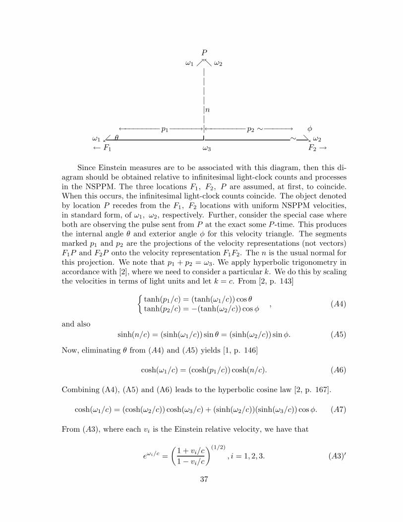
Pω1 ↗↖ ω2

|||||n|

←−−−−−−−−p1−−−−−−→|←−−−−−−−−p2 ∼−−−−−→ φω1 ↙ θ ∼ ↘ ω2

← F1 ω3 F2 →

Since Einstein measures are to be associated with this diagram, then this di-agram should be obtained relative to infinitesimal light-clock counts and processesin the NSPPM. The three locations F1, F2, P are assumed, at first, to coincide.When this occurs, the infinitesimal light-clock counts coincide. The object denotedby location P recedes from the F1, F2 locations with uniform NSPPM velocities,in standard form, of ω1, ω2, respectively. Further, consider the special case whereboth are observing the pulse sent from P at the exact some P -time. This producesthe internal angle θ and exterior angle φ for this velocity triangle. The segmentsmarked p1 and p2 are the projections of the velocity representations (not vectors)F1P and F2P onto the velocity representation F1F2. The n is the usual normal forthis projection. We note that p1 + p2 = ω3. We apply hyperbolic trigonometry inaccordance with [2], where we need to consider a particular k. We do this by scalingthe velocities in terms of light units and let k = c. From [2, p. 143]

{

tanh(p1/c) = (tanh(ω1/c)) cos θtanh(p2/c) = −(tanh(ω2/c)) cos φ

, (A4)

and also

sinh(n/c) = (sinh(ω1/c)) sin θ = (sinh(ω2/c)) sin φ. (A5)

Now, eliminating θ from (A4) and (A5) yields [1, p. 146]

cosh(ω1/c) = (cosh(p1/c)) cosh(n/c). (A6)

Combining (A4), (A5) and (A6) leads to the hyperbolic cosine law [2, p. 167].

cosh(ω1/c) = (cosh(ω2/c)) cosh(ω3/c) + (sinh(ω2/c))(sinh(ω3/c)) cos φ. (A7)

From (A3), where each vi is the Einstein relative velocity, we have that

eωi/c =

(

1 + vi/c

1− vi/c

)(1/2)

, i = 1, 2, 3. (A3)′

37

From the basic hyperbolic definitions, we obtain from (A3)′

tanh(ωi/c) = vi/ccosh(ωi/c) = (1− v2

i /c2)−1/2 = βi

sinh(ωi/c) = βivi/c. (A8)

Our final hyperbolic requirement is to use

tanh(ω3/c) = tanh(p1/c + p2/c) =tanh(p1/c) + tanh(p2/c)

1 + (tanh(p1/c)) tanh(p2/c). (A9)

Now into (A9), substitute (A4) and then substitute the first case from (A8).One obtains

v1 cos θ =v3 − v2 cos φ

1− α, α =

v3v2 cos φ

c2. (A10)

Substituting into (A7) the second and third cases from (A8) yields

β1 = β2β3(1− α), βi = (1− v2i /c2)−1/2. (A11)

From equations (A11), (A5) and the last case in (A8) is obtained

v1 sin θ =v2 sinφ

β3(1− α). (A12)

For the specific physical behavior being displayed, the photons received fromP at F1 and F2 are “reflected back” at the NSPPM P -time tr. We then apply tothis three point scenario our previous results. [Note: For comprehension, it may benecessary to apply certain relative velocity viewpoints such as from F1 the point Pis receding from F1 and F2 is receding from P . In this case, the NSPPM times whenthe photons are sent from F1 and F2 are related. Of course, as usual there is assumedto be no time delay between the receiving and the sending of a “reflected” photon.]In this case, let t(1), r(1), v1 be the Einstein measures at F1 for this P -event, andt(2), r(2), v2 be the Einstein measures at F2. Since tr = β−1

1 t(1), tr = β−12 t(2) (p.

52), thent(1)

β1=

t(2)

β2and r(1) = v1t

(1), r(2) = v2t(2). (A13)

Suppose that we have the four coordinates, three rectangular, for this P eventas measured from F1 = (x(1), y(1), z(1), t(1)) and from F2 = (x(2), y(2), z(2), t(2)) in athree point plane. It is important to recall that the x, y, z are related to Einsteinmeasures of distance. Further, we take the x-axis as that of F1F2. The v3 is theEinstein measure of the F2 velocity as measured by an inf. light-clock at F1. Tocorrespond to the customary coordinate system employed [1, p. 32], this gives

{

x(1) = v1t(1) cos θ, y(1) = v1t

(1) sin θ, z(1) = 0x(2) = −v2t

(2) cos φ, y(2) = v2t(2) sin φ, z(2) = 0

. (A14)

38

It follows from (A10), · · · , (A14) that

t(1) = β3(t(2)− v3x

(2)/c2), x(1) = β3(x(2) − v3t

(2)), y(1) = y(2), z(1) = z(2). (A15)

Hence, for this special case ω1, ω2, θ, φ are eliminated and the Lorentz Trans-formations are established. If P 6= F1, P 6= F2, then the fact that x(1), x(2) are notthe measures for a physical ruler but are measures for a distance related to Einsteinmeasures, which are defined by the properties of the propagation of electromag-netic radiation and infinitesimal light-clock counts, shows that the notion of actualnatural world “length” contraction is false. For logical consistency, Einstein mea-sures as determined by the light-clock counts are necessary. This analysis is relativeto a “second” pulse when light-clock counts are considered. The positions F1 andF2 continue to coincide during the first pulse light-clock count determinations.

Infinitesimal light-clock counts allow us to consider a real interval as an intervalfor “time” measure as well as to apply infinitesimal analysis. This is significantwhen the line-element method in Article 3 is applied to determine alterations inphysical behavior. All of the coordinates being considered must be as they wouldbe understood from the Einstein measure viewpoint. The interpretations mustalways be considered from this viewpoint as well. Finally, the model theoretic errorof generalization is eliminated by predicting alterations in clock behavior ratherthan by the error of inappropriate generalization.

REFERENCES

Dingle, H. The Special Theory of Relativity, Methuem & Co., London, 1950.

Herrmann, R. A. “The NSP-world and action-at-a-distance,” In “InstantaneousAction at a Distance in Modern Physics: ‘Pro’ and ‘Contra,’ ” Edited by Chubykalo,A., N. V. Pope and R. Smirnov-Rueda, (In CONTEMPORARY FUNDAMENTALPHYSICS - V. V. Dvoeglazov (Ed.)) Nova Science Books and Journals, New York,1999, pp. 223-235. Also see http://arxiv.org/abs/math/9903082 pp. 118-119.

Kulczycki, S. Non-Euclidean Geometry, Pergamon Press, New York, 1961.

39