a note on the dirichlet process prior in bayesian - citeseerx

mm7.,,-,~ ,-r ,-..z.,v~,

ELSEVIER Statistics & Probability Letters 36 (1997) 69-83

&

A note on the Dirichlet process prior in Bayesian nonparametric inference with partial exchangeability 1

Sonia Petrone a, Adrian E. Raftery b,*

a Dipartimento di Economia Politica e Metodi Quantitativi, Universita de Pavia 1-27100 Pavia, Baly b Department of Statistics, University of Washinoton, Box 354322, Seattle WA 98195-4322, USA

Received July 1996; received in revised form March 1997

Abstract

We consider Bayesian nonparametric inference for continuous-valued partially exchangeable data, when the partition of the observations into groups is unknown. This includes change-point problems and mixture models. As the prior, we consider a mixture of products of Dirichlet processes. We show that the discreteness of the Dirichlet process can have a large effect on inference (posterior distributions and Bayes factors), leading to conclusions that can be different from those that result from a reasonable parametric model. When the observed data are all distinct, the effect of the prior on the posterior is to favor more evenly balanced partitions, and its effect on Bayes factors is to favor more groups. In a hierarchical model with a Dirichlet process as the second-stage prior, the prior can also have a large effect on inference, but in the opposite direction, towards more unbalanced partitions. (~) 1997 Elsevier Science B.V.

Keywords: Bayesian nonparametric inference; Dirichlet process; Hierarchical model; Partial exchangeability; Partition models

1. Introduction

We consider a Bayesian nonparametric model for partially exchangeable data, when the allocation o f cases to groups is unknown. This includes change-point problems, mixture models and, more generally, can be seen as a nonparametric extension of hierarchical partition models (Consonni and Veronese, 1995, and references therein). As a prior, we consider a mixture of products of Dirichlet processes. This prior has been used by Cifarelli and Regazzini (1978) as a generalization o f the Dirichlet process o f Ferguson (1973, 1974). The peculiarity of the problem we consider is that the partition of the data into groups is unknown and, in fact, is often one of the main objects of inference.

We compute the posterior distributions of the quantities of interest in the proposed model. Our emphasis is on the effects o f the discreteness of the Dirichlet process on inference about the unknown partition (posterior distributions and Bayes factors) in this situation. The phenomenon illustrated here is due to the structure o f

* Corresponding author. I This research was supported by ONR Grants No. N-00014-91-J-1074 and N00014-96-1-0192 and by grants from MURST, Rome.

0167-7152197/$17.00 (~) 1997 Elsevier Science B.V. All rights reserved PH S0 167-7 ! 5 2 ( 9 7 ) 0 0 0 5 0 - 3

70 S. Petrone, A.E. Raftery / Statistics & Probability Letters 36 (1997) 69-83

the distribution of a sample from a Dirichlet process and in this sense it can arise, more generally, in different contexts. For example, it is at the base of the difficulties in using the Dirichlet process prior in goodness of fit testing, pointed out by Carom and Parmigiani (1995).

More specifically, the problem discussed in the paper can be explained as follows: The Dirichlet process almost surely selects a discrete distribution function (d.f.) (Blackwell, 1973; Blackwell and McQueen, 1973). As a result, when used as a prior distribution for a sequence of exchangeable random variables (r.v.'s), it gives positive probability to ties in the data. Nevertheless, the Dirichlet process is also used as a prior in situations where the data are "continuous", i.e., when the probability of ties in the data is very small, or zero. In many situations, the discreteness of the Dirichlet process has no relevant effects. However, in the situation considered in this paper, when the data are partially exchangeable with an unknown partition, it turns out to have a large effect on inferences, in a way that is not clearly part of the prior specification.

When the observed data are all distinct, the effect of the Dirichlet process prior is to favor nearly equally sized groups and to make partitions with very unequally sized groups unlikely a posteriori. It also tends to greatly inflate Bayes factors for more groups against less groups when the number of groups is unknown a priori. Equivalently, it tends to concentrate the posterior distribution of the number of groups on higher values.

Intuitively, the reason is that, when the data are all distinct, the likelihood can be written as the product of two factors: (1) the likelihood under the parametric model that is the mean of the (product of) Dirichlet process(es) prior, and (2) the probability of having no ties in the data. The effect we have observed is due to the second factor: the probability of no ties is higher when the number of groups is bigger, and, given the number of groups, when these are of equal size rather than when they are very unequal, sometimes much more so. What is perhaps surprising is the magnitude of the effect.

This leads to suggestions and warnings about the use of a Dirichlet process prior in this situation. The warning is as follows: If the true distribution is close to the prior mean, we would prefer the posterior distribution from the nonparametric model to be close to that from the parametric model corresponding to the prior mean. However, the presence of the second factor in the likelihood shows that this will not be the case in general, and that the two posterior distributions may be very different. The point that we are making here applies to the situation where the partition into groups is unknown. The discreteness of the Dirichlet process is not so crucial if the partition of data into groups is known, in which case the probability of no ties is a constant depending only on known quantities (Cifarelli and Regazzini, 1978).

In Section 2, we discuss the likelihood of a sample from a Dirichlet process. In Section 3 we illustrate the effect discussed here in the context of a simple change-point problem. In Section 4, we give results for the more general situation of partial exchangeability where the partition is unknown. In Section 5, we make some remarks about the situation where the Dirichlet process is used as a prior at the second stage of a Bayesian hierarchical model. In this situation, the prior can also have a large effect on inference, but in the opposite direction, towards more unbalanced partitions.

2. The likelihood of a sample from a Diriehlet process

Let X1 . . . . . Xn be real valued r.v.'s, which are a sample from a Dirichlet process, i.e., X1 . . . . . Xn ] F are conditionally i.i.d, according to the d.f. F, and F is a Dirichlet process whose parameter is a measure ~: F ~ ~(~). This induces a probability P on the sample space (~n ,~(Rn) ) (Ferguson, 1973). The predictive distribution of Xj IX1 =Xb . . . ,X j -1 = xj_~ for any j = 1 . . . . . n, is

1 P(Xj <~x IX1 =Xl . . . . . Xj-1 = x j - l ) = M + j - 1 ~ ( ( - ° c ' x ] ) +

j - 1 M + j - 1 Fj-l(X)

S. Petrone, A.E. Raftery I Statistics & Probability Letters 36 (1997) 69-83 71

where M = ct(R) and Fj_I is the empirical d.f. o f the first ( j - 1) observations, (xl . . . . ,Xj--1). We will restrict our attention to the case where the parameter ~ is absolutely continuous with respect to the Lebesgue measure 2 on R, with density d~/d2(x) = Mfo(x ) .

From the form of the predictive distribution, proceeding as in Korwar and Hollander (1973) and Antoniak (1974, Lemma 1 ), it can be shown that P, i.e. the joint probability law of (X1 . . . . . X,), gives positive probability to certain collections of hyperplanes in the sample space R ~. Let us introduce the set

Cg(D, nl . . . . . riD) = {(Xl . . . . . X,) : there are D distinct values; one of them is repeated

nl times, one is repeated n2 times . . . . . one is repeated nD times },

where ( n l . . . . . nD) is a sequence of integers such that rt i > 0 , n l ~<n2 ~< " ' " ~nD and ~--~/°=l n i ~- n. An ordering (o) for a sequence (xl . . . . . x , ) E C~(D,n~ . . . . . no) is a subset of the integers (1,2 . . . . . n) showing the positions where a value different from the previous ones appears. For example, if (Xl . . . . . xs) = (1, 1,9, 8, 1 ), the ordering is (1,3, 4), since new values appear in these positions.

Now, let us denote by 2(D;n,,...,no,o) a measure defined on ( ~ , ~ ( ~ ' ) ) which is degenerate on the hyperplane

{(xl . . . . , x , ) E Nn : (x l , . . . ,Xn) E Cg(D, nl . . . . . no) and satisfies the ordering (o)}

and has D-dimensional marginal on the D distinct coordinates coincident with Lebesgue measure on (ND, N(No) ) So, e.g., for n = 3, if (o) denotes the appearance of two distinct values at positions (1,3), 2(2;1,2,o) is a measure o n ( ~ 3 , ~ ( ~ 3 ) ) , degenerate on

{(Xl,X2,X3) E ~3 : Xl = X2 ~ X3},

having Lebesgue measure on ~2 as the marginal of the two distinct coordinates. Since the measures 2(D,n,...,no,o) are defined on the same space, ( ~ n , ~ ( ~ n ) ) , their sum can be defined as

~1(") : ~ Z Z ~(D,nl,...,no,O)("), S E ,~(~n). D : I (nl,...,nD) (O)

It can be shown that P is absolutely continuous with respect to ~b, with derivative

dP

dO - - ( x l . . . . ,Xn) =- f , ( x l . . . . . Xn)

D=I (nh...,no)

MD D D M[n] l - I (ni - 1)[ 1-I f ° (x t i ) I~(D'nl,'",no) (xl . . . . . Xn),

i=l i=l

where M [k] = M ( M + 1 ) . . . (M + k - 1 ) ; M [°] = 1; and (X¢l . . . . . XID) is the vector of distinct values among (xl . . . . . Xn), with x'i repeated ni times. In other words,

MD D D Sn(Xl .. . . ,Xn) = 1-I 1-I So(x',),

i :1 i :1

(1)

if (xl . . . . . x , ) E Cg(D, nt . . . . . no), having D distinct valuesD(x' 1 . . . . . X'D) repeated nl . . . . . nD times. The interpretation of the two components M D / M In] r I i = l ( n i - 1)! and r[D=I fo (x ' i ) of the likelihood (1)

is as follows. The first is the probability that (X1 . . . . . An) belongs to ~(D, nl . . . . . no) and has a given ordering. The second is the joint density of the D distinct values, given the configuration ~(D, nl . . . . . riD); indeed, Korwar and Hollander (1973) show that, given the number D of distinct values, these are i.i.d. according to fo .

72 S. Petrone, A.E. Raftery I Statistics & Probability Letters 36 (1997) 69-83

If 0(1 . . . . . Xn) is a sample from a mixture of Dirichlet processes (Antoniak, 1974), i.e., (X1,...,Xn) are conditionally i.i.d, according to F, F I 0 ~ ~(~(., 0)) and tO ,-~ H(O), and if ct(., 0) is absolutely continuous with respect to Lebesgue measure for any 0, then the likelihood of (xl . . . . . xn J 0) is given, as in (1), by

f n(Xl . . . . . Xn; O) -- ~(~; O)D D D ~(R;0)[n] 1-[ (ni - 1)! I-[ fo(x'i;O). (2)

i=1 i=1

This differs slightly from Lemma 1 of Antoniak (1974), but only in the specification of the dominating measure.

3. A simple change-point example

3.1. Posterior distribution of the change point

To illustrate the general phenomenon, we will describe how it affects inference for a simple change-point problem. Data (X1 . . . . ,Xn) are assumed to arise from the model

X/ '~F1, i = 1,. . . ,C,

X~ ,'~ F2, i = C + I . . . . . n,

where C is the change point, which is unknown. Nonparametric Bayesian inference is carried out by assigning (mixture of) Dirichlet process priors to F1 and F2.

The model can be written

C n P(X1 ~ X l , X 2 ~x2 . . . . . Xn ~x . lg , FhF2) = I] ]I Fz(x,), (3)

i=1 i=C+I

where C is the unknown change point. This means that the observations are conditionally i.i.d, according to F1 up to time C and i.i.d, according to F2 from time (C + 1) on. When C = 0 or C = n there is no change point and the data are conditionally i.i.d, as F2, or F1, respectively.

The prior assumes that C and (Fa,F2) are independently distributed, C with probability mass function p(c) and (FI,F2) as a mixture of products of Dirichlet processes (Cifarelli and Regazzini, 1978). The prior distribution is, thus,

f ~ (0~1 ('; 01 )) ,~ (Gt2 ('; 02)) d/-/(01,02)- (4) (El,F2, C) p(c)

This model has been studied by Muliere and Scarsini (1985) in the special case of independent F1 and F2. A Gibbs sampler algorithm for approximating the posterior distributions in the above model is provided in Mira and Petrone (1995). On the lines of Section 2, it can be shown that, when ~1(.;01) and ~2(';02) have densities M l f l (.; 01 ) and Mzf2(-; 0z), respectively, with respect to Lebesgue measure, the likelihood is

1 I-iMlfl(Xi;O1) 1 f (X l ,X2 . . . . . Xn I c, OI.02,) = ~ ~.r[n-c'---""-~ M2f2(x i ;02) , (5) 1vl i - i=1 i=c+l

where the • indicates that the product is taken over distinct values only. From (5) the posterior distribution of (C, 0~, 02) can be computed by applying Bayes' theorem. In particular,

in the continuous case and if the observations (Xl . . . . . Xn) are all distinct, we have

p(c Ix1 . . . . . x , ) cx k(e, M1,M2,n) I(c) p(c), (6)

S. Petrone, A.E. Raftery / Statistics & Probability Letters 36 (1997) 69-83 73

where, for c -- 0, 1 . . . . . n, we let

l(c) = f r i f l (x i ;o l ) fz(xi;O2)dH(Ol,O2), i=1 i=c+l

and

- M c1 M ,_cl.

The factor k(c, M1,M2,n) is the probability of there being no ties in the data, given that C = c. The probability of the data values all being distinct is

" ~ M~ -1 ""2AAn-~-I ~P(X~ ¢X2 ¢ - . . CX, Ic) p(c)-- (M1 + 1)t~-ll (M2 + 1)t~-~-~l p(c) c=0 c=0

R C ?I--C

~ p(c)

= ~ k(c, ml,M2,n) p(c). c=0

We note that the posterior (6) is equivalent, except for the factor k(c, M1,M2,n), to what we obtain with the parametric model where (Xl . . . . . Xn) have the joint conditional density

f (X l . . . . . Xn Ic, 01,02)= I-I f I(X';O1) r I f2(xi;02)" ( 7 )

i=1 i=r+l

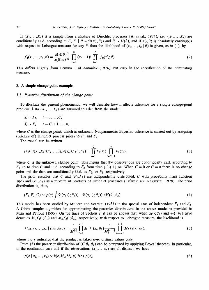
Here, I(c) is the (integrated) likelihood of c, and the posterior is given by (6) with k(c, M1,M2,n) = 1. The factors k(c;M1,M2,n) are plotted in Fig. 1 for the nonparametric model with Ml = M2 = 1, and sample

sizes n = 10 and 50.The plots show that k(c;Mi,M2,n) is much bigger for values of c close to n/2, and that this behavior is more marked if n is larger. For the parametric model (7), in contrast, k(c, M1,M2,n) = 1, a constant. When M1 and M2 are very large, corresponding to a large amount of prior information, this effect is attenuated, since for M1,M2 ~ +c~, (6) converges to the parametric result.

3.2. Bayes factors

Suppose we want to test the hypothesis of no change-point against the alternative that one change-point occurred. In our model, these hypotheses are expressed by: H0 : C E {0,n) and H1 : C E {1,2 . . . . . n - 1}. For this problem, we can compute the relevant Bayes factor (see Kass and Raftery, 1995 for a review).

The Bayes factor for H0 versus H1 is

BOl = )--]~{c=O,.} f (xlc)p°(c) , (8) n - I

~c=1 f(x_ l c)pl(c)

where

po(c) = { p(c) for c = O, n,

p(O) + p(n)

0 otherwise,


I

f ~

Q

• •

O 0 q

0 2 4 6 8 10

o o

Y, '~ °

t ' 3

° I 0J

tO • ° o

n

o . . . . . . . . . o

o 2o

o

o

o

°o . . . . . . . . . . . . .

40 60

(~) (b)

Fig . 1. P lo t o f fac tors k(c, MbM2,n), fo r M1 = M2 = 1; n = 10 and n = 50.

and

p(c) for c = 1 , . . . , n - 1, pl(c) = E~-~ p(c)

0 otherwise.

In the continuous case, with (xl, . . . ,Xn) all distinct, the Bayes factor is given by

B0, = ~{c=0,n} po(e) k(c, Mi,M2) I(c) (9) ~--~-~ pl(c) k(c,M,,M2) I(c)

As for the posterior distribution, the Bayes factor (9) is equivalent, except for the factor k(c, Ml,M2,n), to what we obtain with the parametric model (7); indeed, in the parametric case the Bayes factor is given by (9) with k(c, M b M 2 , n ) = 1. For a review of the Bayesian analysis of parametric change-point problems, see Raflery (1994).

3.3. A numerical example

In the simple nonparametric change-point model of the previous sections, let f i ( . ,O i ) be a normal density with mean Oi and known variance Z 2, 01 and 02 be independent and normally distributed, with Oi

1 N(#i, zi) i = 1,2;, and let p(c) be chosen so that: p ( 0 ) + p(n) = p (1 )+ . . .+ p ( n - 1 ). This gives probability to each of the two hypotheses: (no change-point: c E {0, 1 }) and (a change-point occurred: c E { 1 . . . . . n - 1 }), with p(0) -- p(n) and p(1) . . . . . p(n - 1). We fix a = 1,Zl = z2 = 1,/~l = 5,/~2 = 8,MI =M2 = M and consider varying values of M. Also, let Nk(p, S) denote the k-variate normal density with mean vector/ , and covariance matrix Z, Ik = (1, . . . , 1) p be the (k × 1) vector of ones, Jk be the (k x k) matrix every element of which is unity, and Ik be the k-dimensional identity matrix.

Then it can be shown (Muliere and Scarsini, 1984) that 1(c) is the product of two normal densities: Nc(Itl , Zc ) and Nn_c(la2, Zn_c ), computed from (X 1 . . . . . Xc ) and (Xc + l . . . . . Xn ) respectively, where

zc = ~2I~ + ~J~


t-w

o

o o o

0 5 10 15 2 0

Fig. 2. Data: 20 observations from a translated Student's t distribution with two degrees of freedom.

0

n ?

t ' q

a

5 10 15 2 0 0 5 10 15 2 0

(~) (b)

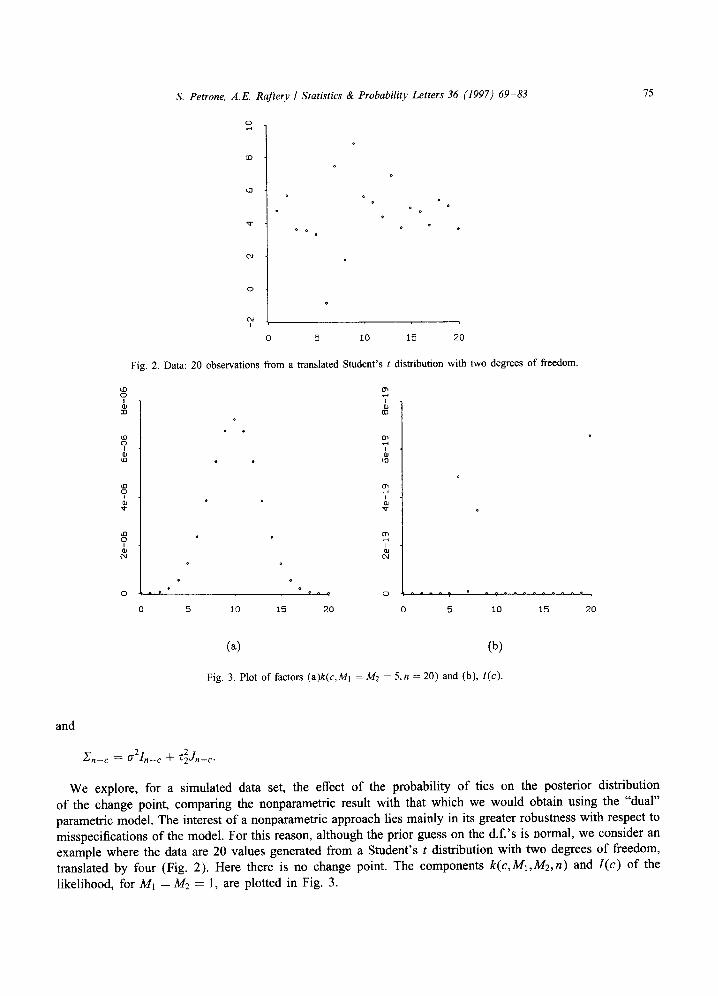
Fig. 3. Plot of factors (a)k(c, Ml = M2 = 5,n = 20) and (b), l(c).

and

Zn--c ~-" 0"2 In--c -~- g~Jn-c.

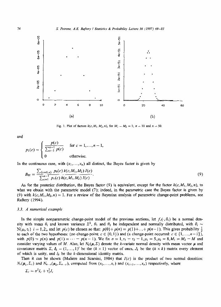
We explore, for a simulated data set, the effect o f the probability of ties on the posterior distribution of the change point, comparing the nonparametric result with that which we would obtain using the "dual" parametric model. The interest o f a nonparametric approach lies mainly in its greater robustness with respect to misspecifications of the model. For this reason, although the prior guess on the d.f.'s is normal, we consider an example where the data are 20 values generated from a Student's t distribution with two degrees o f freedom, translated by four (Fig. 2). Here there is no change point. The components k(c, M1,M2,n) and l (c) of the likelihood, for M1 = M2 --- l, are plotted in Fig. 3.


~D

0

(3

0 5 I0 15 20 0 5 I0 15 20

(~) (b)

Fig. 4. Posterior distribution of the changepoint: (a) nonparametric model, Ml = M2 = 1; (b) parametric model.

Table 1 Bayes factors for H0: no change, against Hi: a change point occurred

Bayes factor

Parametric model 7.3 Nonparametric model, M = 1 0.00018 Nonparametric model, M = 5 0.011

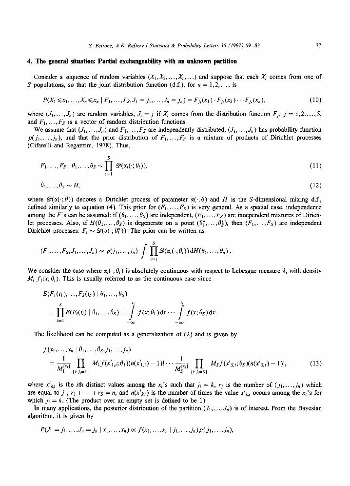
The parametric (integrated) likelihood, I(c), provides some evidence for the change point being at one of the times 20 (i.e. no change), 6 or 8. The parametric posterior distribution (with a prior for c that gives equal total weight to times representing no change as to times representing a change) is shown in Fig. 4(b). This is mostly concentrated on c = 20 (i.e. no change point). The nonparametric posterior distribution in Fig. 4(a) is very different. It suggests that there was almost certainly a change point at one of the times 6-8, and gives no weight at all to c = 20.

The same phenomenon affects the Bayes factor, as shown in Table 1. For the parametric model, the Bayes factor for no change is about 7.3, providing positive evidence against a change point. For the nonparametric model with M = 1, the Bayes factor is about 5000:1 for a change - a very misleading conclusion, and dramatically different from that based on the parametric model. For M = 5 the effect is less dramatic, but still strong.

The posterior distribution of the change point also affects the estimates of the distribution functions before and after the change. The estimate of Fi(t) (i = 1,2) is the average, with respect to the posterior of C, of the conditional expected value of Fi(t) given the data and C = c. In the nonparametric case, the conditional expected value ofFi( t) lC, Xl . . . . . Xn is a weighted average between the prior guess about Fi(t) and the empirical d.f. of the first c observations. One would hope that the component due to the empirical d.f.'s would result in a more robust estimate, compared with that obtained with a strict parametric assumption. Yet, the nonparametric estimate of Fi, being an average with respect to p(c [xl,. . . ,xn), will depend on the probabilities of ties.


4. The general situation: Partial exchangeability with an unknown partition

Consider a sequence of random variables (X1,X2 . . . . . X, . . . . ) and suppose that each X/ comes from one of S populations, so that the joint distribution function (d.f.), for n = 1,2 . . . . . is

P(X1 <.xl . . . . . Xn <~Xn I F1 . . . . . Fs,J1 = j l . . . . . Jn = Jn) = Fj,(Xl )" F j , ( x2 ) "" Fj,(Xn), (10)

where (Jl . . . . . Jn) are random variables, Ji = j if X/ comes from the distribution function Fj, j = 1,2 . . . . . S, and F1 . . . . . Fs is a vector of random distribution functions.

We assume that (Jl . . . . . Jn) and F1 . . . . . Fs are independently distributed, (.Ix . . . . . Jn) has probability function P( j l . . . . . jn), and that the prior distribution of F1 . . . . . Fs is a mixture of products of Dirichlet processes (Cifarelli and Regazzini, 1978). Thus,

S

F1 . . . . . Fs I 01 . . . . . Os ~ I X ~(o~i(';Oi)), i=1

(11)

01 . . . . . O s ~ H , (12)

where ~(~(.; 0)) denotes a Dirichlet process of parameter a(.; 0) and H is the S-dimensional mixing d.f., defined similarly to equation (4). This prior for (Fl . . . . ,Fs) is very general. As a special case, independence among the F ' s can be assumed: if (01 . . . . . Os) are independent, (F1 . . . . . Fs) are independent mixtures of Dirich- let processes. Also, if H(O1 . . . . . Os) is degenerate on a point (0~' . . . . . 0]), then (F1 . . . . . Fs) are independent Dirichlet processes: F i ' ~ ~(~( ' ; 0")). The prior can be written as

(F1 . . . . . Fs,J1 . . . . . Jn) ~ P(jl . . . . . jn)

S

f i x d/-/(01 .... . 0.). i=1

We consider the case where ~i(.; Oi) is absolutely continuous with respect to Lebesgue measure 2, with density Mi f i (x ; Oi). This is usually referred to as the continuous case since

E(F1(t l) . . . . . Fs( ts) I Ox . . . . . Os)

S fi ts

i=l --o~ --oo

The likelihood can be computed as a generalization of (2) and is given by

f ( x l . . . . . Xn 101 . . . . . Os,jl . . . . . jn)

1 -- M[rO :P,= Ml f (X ' l , i ;O1)(n(x ' l , i ) - l)''"Mirs---~ 1-I

{, 1} { i : j i=S}

m / ! s f ( x s,i; Os)(n(x s,i) - 1)!, (13)

where x'k,i is the ith distinct values among the xi's such that j i = k, rj is the number of (J1 . . . . . j , ) which are equal to j , rl + . . . + rs = n, and n(x'k,i) is the number of times the value xlk,i occurs among the xi's for which ji = k. (The product over an empty set is defined to be 1).

In many applications, the posterior distribution of the partition (./1 . . . . . J , ) is of interest. From the Bayesian algorithm, it is given by

P(JI = j l . . . . . .In = jn I Xl . . . . . Xn) c< f ( x l . . . . . Xn I Jl . . . . . j n ) P ( j l . . . . . jn),


where

. . . . . Xn l J1 . . . . . j , ) = f f ( x l . . . . . Xn [ j l . . . . . jn, O1 . . . . . OS) dn(01 . . . . . Os). f ( x l

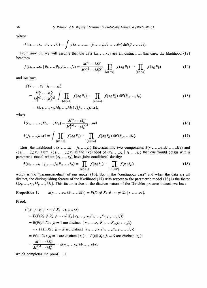
From now on, we will assume that the data (xl . . . . ,Xn) are all distinct. In this case, the l ikelihood (13) becomes

M r , o .oMs S f ( x l . . . . . xn]Ol . . . . . Os,jl . . . . 'Jn)-- .Ar 'O ~¢[rs] I-[ f ( x i ; O l ) " " 1--[ f (x i ;Os) (14)

M r " ' ""aS {i:ji=l} {i:ji=S}

and we have

f (Xl . . . . . Xn I J~ . . . . . J . )

where

M ~ ' ' " M s S / - -M[r ,] :-M--ffsrS] 1-[ f ( x i ; O 1 ) " " I I f ( x i ; O s ) dH(O1 . . . . . On) (15)

{i:j,=l} {i:ji=S}

= k(rl . . . . . rs;M1 . . . . . Ms) 1(jl . . . . . jn;X),

• . .M~ s k ( r l . . . . . rs;M, . . . . . M s ) - M~r" d . . M~rS ] , and

I ( j l . . . . . jn;x)=/ I I f ( x i ;O1)"" H {i:ji=l } {i:j,=S}

f (xi; Os ) dH( 01 . . . . . On).

(16)

(17)

Thus, the l ikelihood f ( x l . . . . . xn [ j l . . . . . jn) factorizes into two components: k(rl . . . . . rs;M1 . . . . . Ms) and I ( j l . . . . . jn;x) . Here, l ( j l . . . . . jn ;x ) is the l ikelihood o f (xl . . . . . Xn l j l . . . . . j , ) that one would obtain with a parametric model where (xl . . . . . Xn) have joint conditional density:

h(Xl . . . . . x n l j l . . . . . jn, O1 . . . . . On)= ]-I f ( x i ; O , ) ' ' " I I f (xi;Os), (18) { i:j,= l } { i:ji=S }

which is the "parametric-dual" o f our model (10). So, in the "continuous case" and when the data are all distinct, the distinguishing feature o f the l ikelihood (15) with respect to the parametric model (18) is the factor k(rl . . . . . rs;Ml . . . . . Ms). This factor is due to the discrete nature o f the Dirichlet process; indeed, we have

Proposi t ion 1. k(rl . . . . . rs;M1 . . . . . Ms) = P(X1 ~ X2 ~ "'" ~ Yn ] rl . . . . . rs).

Proof.

P(X1 (: X2 ( : " " :/: X , I r l . . . . . rs)

= E(P(X1 ¢ X 2 • " " e Xn [ rl . . . . . rs,Fl . . . . . Fs , j l . . . . . jn))

= E(P(aI1X, : ji = 1 are distinct Jr1 . . . . . rs,F1 . . . . . Fs , j l . . . . . j , )

• . . P(a l l X/ : ji = S are distinct [ rl . . . . . rs,Fl . . . . . Fs , j l . . . . . j , ) )

= P(al l X/ : ji = 1 are distinct [ r l ) . . . P(a l l X / : j i = S are distinct [ r s )

M e ' . . . M ; s -- M[rd .MistS ] = k(rl . . . . . rs; M1 . . . . . Ms),

which completes the proof. []

S. Petrone, A.E. Rafter), I Statistics & Probability Letters 36 (1997) 69 -83

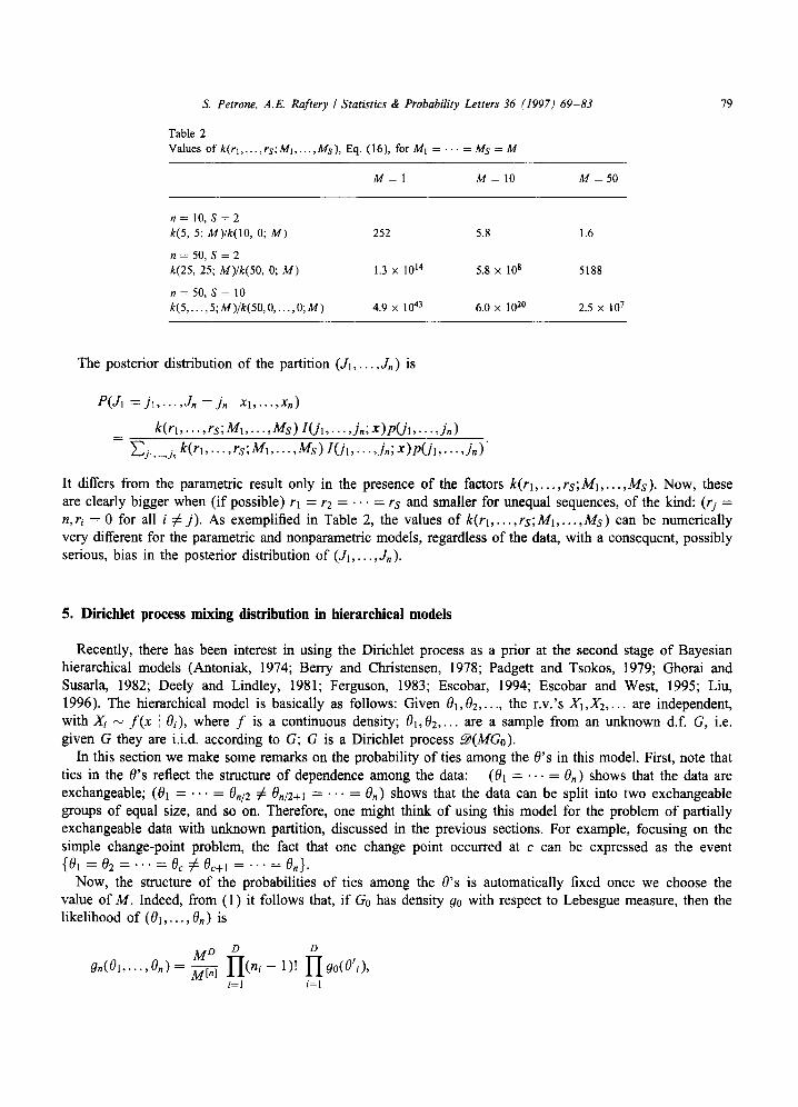
Table 2 Values of k(rl . . . . , rs;Ml . . . . . Ms), Eq. (16), for M1 . . . . . Ms = M

M = 1 M = 10 M = 50

79

n = 1 0 , S = 2 k(5, 5; M)/k(lO, 0; M) 252 5.8 1.6

n = 5 0 , S = 2 k(25, 25; M)/k(50, 0; M) 1.3 × 1014 5.8 x 108 5188

n = 5 0 , S = 1 0 k(5 . . . . . 5;M)/k(50, O . . . . . 0;M) 4.9 × 1043 6.0 × 1020 2.5 × 107

The posterior distribution of the partition (J1 . . . . . Jn) is

P(JI = j l . . . . . Jn = jn IX1 . . . . . Xn)

k(r l . . . . . rs;M1 . . . . . M s ) I ( j l . . . . . jn; x ) p ( j l . . . . . j n )

~j , , ._ , j° k (r l . . . . . rs; M1 . . . . . M s ) I ( j l , . . . , jn; x ) p ( j l . . . . . jn )"

It differs from the parametric result only in the presence of the factors k(r l . . . . . r s ; M l , . . . , M s ) . Now, these are clearly bigger when (if possible) rl = r2 . . . . . rs and smaller for unequal sequences, of the kind: (rj = n, ri = 0 for all i ~ j) . As exemplified in Table 2, the values of k(r l . . . . . rs;M1 . . . . . M s ) can be numerically very different for the parametric and nonparametric models, regardless of the data, with a consequent, possibly serious, bias in the posterior distribution of (J1 . . . . . Jn).

5. Diriehlet process mixing distribution in hierarchical models

Recently, there has been interest in using the Dirichlet process as a prior at the second stage of Bayesian hierarchical models (Antoniak, 1974; Berry and Christensen, 1978; Padgett and Tsokos, 1979; Ghorai and Susarla, 1982; Deely and Lindley, 1981; Ferguson, 1983; Escobar, 1994; Escobar and West, 1995; Liu, 1996). The hierarchical model is basically as follows: Given 01,02 .. . . . the r.v.'s X1,X2 . . . . are independent, with X, ~ f ( x [ Oi), where f is a continuous density; 01,02 . . . . are a sample from an unknown d.f. G, i.e. given G they are i.i.d, according to G; G is a Dirichlet process ~ ( M G o ) .

In this section we make some remarks on the probability of ties among the O's in this model. First, note that ties in the O's reflect the structure of dependence among the data: (01 . . . . . 0n) shows that the data are exchangeable; (01 . . . . . On~2 ~ On/2+l . . . . . On) shows that the data can be split into two exchangeable groups of equal size, and so on. Therefore, one might think of using this model for the problem of partially exchangeable data with unknown partition, discussed in the previous sections. For example, focusing on the simple change-point problem, the fact that one change point occurred at c can be expressed as the event {01 = 02 . . . . . 0c ¢ 0c+1 . . . . . On}.

Now, the structure of the probabilities of ties among the O's is automatically fixed once we choose the value of M. Indeed, from (1) it follows that, if Go has density go with respect to Lebesgue measure, then the likelihood of (01 . . . . . On) is

M D D D

On(O1 . . . . . 0 , , ) = H(n - Hoo(O' ), i=1 i=1


where D is the number of distinct values among (81 . . . . , On) , ( 8 ' 1 . . . . . OtD) is the vector of distinct values and n~ is the number of times the value 0'~ occurs. The probability of a sequence in the subset Cg(D, nl . . . . . no) of the parameter space, having a given ordering, is

MO o H (ni - 1)!. (19) M[n] i=1

The number of such sequences is

n! 1

n l ! . . . n o ! m l ! . . . m n ! '

where mi = number of (nl . . . . ,nD) which are equal to i. It follows that the probability of the configuration C~(D, nl . . . . . nD) is

M D n! 1 (20) P(Cg(D, nl . . . . . r i D ) ) - M[n] nl ...riD ml! ...ran!"

The probability (20) corresponds to formula (4) in Antoniak (1974), noting that nl n 2 . . . n o = 1 m~ 2 m2''" n m". Given the number of distinct values, the prior tends to favor unbalanced partitions over partitions in groups

of equal size. For example, in the change-point problem, the prior probability that a change point occurred at c, c = 1,2 . . . . . n - 1, is, from (19),

M 2 P(01 . . . . . Pc ~ 0c+1 . . . . . On) = ~ (c - 1)! (n - c - 1)!

and, e.g., we have (for even sample size n)

P(01 . . . . . 0n/2 ~ 0n/2+1 . . . . . On) = (n/2 - 1)! (n/2 - 1)!

e(01 . . . . . 0n-1 ¢ On) (n - 2)!

Fixing to fixing share the

(21)

(D, nl . . . . , riD) and the order (o) according to which the D distinct values are located, is equivalent a partition of {1,2 . . . . . n} into D groups Gj = Gj(D, nl . . . . . riD, O), such that the Oi's with i E Gj same value O'j, j = 1, 2 . . . . . D. Then, we can let

n L(X1 . . . . . xn;D,n, . . . . . riD, O) =- f 1-I f(xi l O,)dg.(01 .... '0.)

i = l

MD D / - Mtnl 1-I (ni - 1)!

j=l iEGj(D,nl ,...,riD,O)

where the first integral is over the set

{ (81 . . . . . O n) E Cg(D, nl . . . . . no) which are ordered according to (o)}.

It follows that

n

f ( x l . . . . . xn) =-- / I-[ f ( x i I Oi)dgn(O1 . . . . . On) i=1

~-~-~ E E Z(xa . . . . ,xn;O, nl . . . . . riD, O). D=1 (nb...mD) (O)

H f ( x i l O ' j ) go(O'j)d(O'j), (22)

(23)


The posterior distribution of (01 . . . . . On I x b . . . , X n ) is

g ( 0 1 . . . . . O n IXl , . . . ,Xn) O( I I f ( x i I Oi) gn(O1 . . . . . On)" i=1

Therefore, it depends on the probability of ties, which appears in 9n(O1 . . . . , On) and in the normalizing constant (23). In particular, the posterior distribution of the number D of distinct values among (01,...,0n) is

P ( D = d I xl . . . . . xn) = i dg(Ol . . . . . On Ix1 . . . . . Xn)

{(or, ..., 0 . ) :D=d }

}--]~(nt,...,n~) ~(o)L(Xl . . . . . xn;d, nl . . . . . na, o) (24)

n

~ D = I E(n,,...,nD) ~"~(o) L(Xl . . . . . xn;D, nl . . . . . riD, O)

Expressions (23) and (24) generalize results provided by Liu (1996, Theorems 1 and 2) for the beta-binomial case.

In the change-point problem, we can compute the posterior probability that one change point occurred at C, a s

P(OI . . . . . Oc ¢ Oc+l . . . . . On I xl . . . . . Xn)

{sn iH }" oc f(xi I go(Otl)dO'l f ( x i I Ot2)Oo(Ot2)dOt2 ~ (c - 1)! (n - c - 1)!. i=l i = c + l

The part in brackets is proportional to the posterior of (C, 0'1,0'2) that one would obtain for a parametric model of the kind (7), with 0'i and 0'2 i.i.d, according to 90 and p ( c ) uniform. The second factor is the

0

r l

,:5

o 0 _ _

t

I 0

g d

¢::i

~. o

0

• • • O ~ ~ i Q • o

i i i i i ~ i u

2 4 6 8 0 10 20 30 40 50

Change Point Change Point

Fig. 5. Plot of the factors introduced by the prior in the hierarchical model for M1 = M2 = 1; n == 10 and n = 50.

82 S. Petrone, A.E. Raftery / ,Statistics & Probability Letters 36 (1997) 69-83

prior probability (21) o f one change point at c. In this sense, the posterior probabilities of the change point have a structure similar to (6), with a factor (here M 2 / M In] ( c - 1)! ( n - c - 1)! ) which is part o f the prior and can have a large effect on inference and Bayes factors.

To see this, consider Fig. 5, which shows examples o f these factors contributed by the prior. There are for the same situations as those considered in Fig. 1, with which they can be compared. Clearly, the prior can bias estimation results strongly towards unbalanced partitions.

When using a Dirichlet process for the mixing distribution, the researcher needs to be aware o f this aspect. This is also discussed by Escobar and West (1995), who consider, in addition, the possibility of including uncertainty about M in the model; see also Liu (1996).

6. Discussion

We have shown that when the data are continuous and partially exchangeable with an unknown partition, use o f a Dirichlet process prior can have a large effect on inferences in an unanticipated way.

This is an example o f a case where nonparametric analysis is not robust to the form of the prior. The problem, in our context, seems due to the discrete nature o f the Dirichlet process. Presumably, a more robust nonparametric model would be obtained using a prior incorporating the available information that ties in data will not happen, i.e., a prior that selects a continuous distribution. Unfortunately, in the Bayesian literature there are not many proposals o f priors which are well suited for nonparametric analysis (i.e., which have "large" support on the class o f d.f. 's on the sample space) and which select continuous distributions. In the previous section, we discussed a hierarchical model with X/ [ Oi ~ f ( x [ Oi), and with a Dirichlet process as a prior for the parameters at the second stage. However, as we argued, this solution can also not be robust. Other possibilities include Polya trees priors (Mauldin et al., 1992; Lavine, 1992, 1994), which can be specified to select an absolutely continuous distribution, or, for data in a closed bounded interval, Bemstein priors (Petrone, 1995).

Acknowledgements

The authors are grateful to Peter Green for interesting discussions about the problem treated in Section 5 and to an anonymous referee for helpful comments.

References

Antoniak, C.E., 1974. Mixtures of Dirichlet processes with applications to Bayesian nonparametric problems. Ann. Statist. 2 (6), 1152-1174.

Berry, D.A., Christensen, R., 1979. Empirical Bayes estimation of a binomial parameter via mixtures of Dirichlet processes. Ann. Statist. 3, 558-568.

Blackwell, D., 1973. Discreteness of Ferguson selection. Ann. Statist. 1, 356-358. Blackwell, D., Mac Queen J.B., 1973. Ferguson distributions via Polya scheme. Ann. Statist. 1, 353-355. Carota, C., Parmigiani, G., 1996. On Bayes factors for nonparametric alternatives. In: Bernardo J.M., Berger J.O., Dawid A.P., Smith

A.F.M., (Eds.), Bayesian Statistics, vol. 5. Oxford University Press, Oxford, pp. 507-511. Cifarelli, D.M., Regazzini, E., 1978. Problemi statistici nonparametrici in condizioni di scambiabilita/t parziale. Impiego di medie

associative Quaderni dell'Istituto di Matematica Finanziaria. dell' Universit~ di Torino Serie III, pp. 1-36. Consonni, G., Veronese, P., 1995. A Bayesian method for combining results from sevaral binomial experiments. J. Amer. Statist. Assoc.

90, 935-944. Deely, J.J., Lindley, D.V., 1981. Bayes empirical Bayes. J. Amer. Statist. Assoc. 76, 833-841. Escobar, M.D., 1994. Estimating normal means with a Dirichlet process prior. J. Amer. Statist. Assoc. 89, 268-277. Escobar, M.D., West, M., 1995. Bayesian density estimation and inference using mixtures. J. Amer. Statist. Assoc. 90, 577-587.


Ferguson, T.S., 1973. A Bayesian analysis of some nonparametric problems. Ann. Statist. 1 (2) 209-230. Ferguson, T.S., 1974. Prior distributions on spaces of probability measures. Ann. Statist. 2, (4) 615~529. Ferguson, T.S., 1983. Bayesian density estimation by mixtures of normal distributions. In: Rizvi H., Rustagi J., (Eds.), Recent Advances

in Statistics. Academic Press, New York, 287-302. Ghorai, J.K., Susarla, V., 1982. Empirical Bayes estimation of probability density function with Dirichlet process prior. In: Grossmann,

W., et al. (Eds.), Probability and Statistical Inference. Reidel, Dordrecht, pp. 101-114. Kass, R.E., Raftery, A.E., 1995. Bayes factors. J. Amer. Statist. Assoc. 90, 773-795. Korwar, R.M., Hollander, M., 1973. Contribution to the theory of Dirichlet processes. Ann. Probab. 1, 705-711. Lavine, M., 1992. Some aspects of Polya tree distributions for statistical modelling. Ann. Statist. 20, 1222-1235. Lavine, M., 1994. More aspects of Polya tree distributions for statistical modelling. Ann. Statist. 22, 1161-1176. Liu, J.S., 1996. Nonparametric hierarchical Bayes via sequential imputation. Ann. Statist. 24 (3), 911-930. Mauldin, R.D., Sudderth, W.D., Williams, S.C., 1992. Polya trees and random distributions. Ann. Statist. 20 (3), 1203-1221. Mira, A., Petrone, S., 1996. Bayesian hierarchical nonparametric inference for changepoint problems. Bernardo J.M., Berger J.O., Dawid

A.P., Smith A.F.M., (Eds.), Bayesian Statistics vol. 5. Oxford University Press, Oxford, 693-703. Muliere, P., Scarsini, M., 1984. Bayesian inference for change-point problems. Riv. Statist. Appl. 17, 93-102. Muliere, P., Scarsini, M., 1985. Changepoints problems: a Bayesian nonparametric approach. Appl. Math., 30, 397-402. Padget, W.J., Tsokos, C. T., 1979. Bayes estimation of reliability using an estimated prior distribution. Oper. Res. 27, 1142-1157. Petrone, S., 1995. Random Bernstein polynomials. Quaderni di Dipartimento 30 (12-95), Dipartimento di Economia Politica e Metodi

Quantitativi, Universitfi di Pavia, Raftery, A.E., 1994. Change point and change curve modeling in stochastic processes and spatial statistics. J. Appl. Statist. Sci. 1,

403-424.

a note on the dirichlet process prior in bayesian - citeseerx

Documents