sustainability

Article

A Novel Hybrid Evolutionary Data-IntelligenceAlgorithm for Irrigation and Power ProductionManagement: Application to Multi-PurposeReservoir Systems

Zaher Mundher Yaseen 1 , Mohammad Ehteram 2, Md. Shabbir Hossain 3 , Chow Ming Fai 4,Suhana Binti Koting 5, Nuruol Syuhadaa Mohd 5, Wan Zurina Binti Jaafar 5,Haitham Abdulmohsin Afan 5,*, Lai Sai Hin 5, Nuratiah Zaini 6, Ali Najah Ahmed 4 andAhmed El-Shafie 5

1 Faculty of Civil Engineering, Ton Duc Thang University, Ho Chi Minh City, Vietnam; yaseen@tdtu.edu.vn2 Department of Water Engineering and Hydraulic Structures, Faculty of Civil Engineering,

Semnan University, Semnan 35131-19111, Iran; mohammdehteram@semnan.ac.ir3 School of Energy, Geoscience, Infrastructure and Society, Department of Civil Engineering,

Heriot-Watt University, Putrajaya 62200, Malaysia; m.hossain@hw.ac.uk or realism007@gmail.com4 Institute of Energy Infrastructure (IEI), Civil Engineering Department, Universiti Tenaga Nasional,

Kajang 43000, Selangor, Malaysia; chowmf@uniten.edu.my (C.M.F.); mahfoodh@uniten.edu.my (A.N.A.)5 Civil Engineering Department, Faculty of Engineering, University of Malaya, Kuala Lumpur 50603,

Malaysia; suhana_koting@um.edu.my (S.B.K.); n_syuhadaa@um.edu.my (N.S.M.);wzurina@um.edu.my (W.Z.B.J.); laish@um.edu.my (L.S.H.); elshafie@um.edu.my (A.E.-S.)

6 Department of Civil Engineering, College of Engineering, Universiti Tenaga Nasional, Kajang 43000,Selangor, Malaysia; Nur_Atiah@uniten.edu.my

* Correspondence: haitham.afan@gmail.com

Received: 25 December 2018; Accepted: 19 February 2019; Published: 2 April 2019�����������������

Abstract: Multi-purpose advanced systems are considered a complex problem in water resourcemanagement, and the use of data-intelligence methodologies in operating such systems providesmajor advantages for decision-makers. The current research is devoted to the implementation ofhybrid novel meta-heuristic algorithms (e.g., the bat algorithm (BA) and particle swarm optimization(PSO) algorithm) to formulate multi-purpose systems for power production and irrigation supply.The proposed hybrid modelling method was applied for the multi-purpose reservoir system ofBhadra Dam, which is located in the state of Karnataka, India. The average monthly demand forirrigation is 142.14 (106 m3), and the amount of released water based on the new hybrid algorithm(NHA) is 141.25 (106 m3). Compared with the shark algorithm (SA), BA, weed algorithm (WA),PSO algorithm, and genetic algorithm (GA), the NHA decreased the computation time by 28%, 36%,39%, 82%, and 88%, respectively, which represents an excellent enhancement result. The amountof released water based on the proposed hybrid method attains a more reliable index for thevolumetric percentage and provides a more effective operation rule for supplying the irrigationdemand. Additionally, the average demand for power production is 18.90 (106 kwh), whereas theNHA produces 18.09 (106 kwh) of power. Power production utilizing the NHA’s operation ruleachieved a sufficient magnitude relative to that of stand-alone models, such as the BA, PSO, WA,SA, and GA. The excellent proficiency of the developed intelligence expert system is the resultof the hybrid structure of the BA and PSO algorithm and the substitution of weaker solutions ineach algorithm with better solutions from other algorithms. The main advantage of the proposedNHA is its ability to increase the diversity of solutions and hence avoid the worst possible solutionsobtained using BA, that is, preventing a decrease in local optima. In addition, the NHA enhances theconvergence rate obtained using the PSO algorithm. Hence, the proposed NHA as an intelligence

Sustainability 2019, 11, 1953; doi:10.3390/su11071953 www.mdpi.com/journal/sustainability

Sustainability 2019, 11, 1953 2 of 28

model could contribute to providing reliable solutions for complex multi-purpose reservoir systemsto optimize the operation rule for similar reservoir systems worldwide.

Keywords: hybrid expert system; bat algorithm; particle swarm optimization algorithm; multi-purposesystem; water resource management

1. Introduction

Water resource management attempts to control water scarcity during successive droughtperiods [1]. Climate change phenomena and increasing population demands cause serious naturaldilemmas that necessitate the operation of an optimal and reliable system for managing waterresources [2–4]. The optimal operation of stored water resources in the form of reservoirs behinddams is an important and complicated issue for decision-makers and designers worldwide, becauseoptimal operations can decrease the expenditure of constructing large dams for policymakers in thewater resource management field [5]. Thus, several studies have investigated the optimal operation ofreservoirs to satisfy downstream consumer demands and supply water based on high certainty [6–8].Recently, mathematical models and evolutionary algorithms have been used in the management andplanning of water resources [9–12]. The problem with optimal operations related to water reservoirs canbe defined within the framework of an optimization problem [13–15]. Thus, meta-heuristic algorithms,which are powerful tools, are used for solving such problems [16]. The water supply problemincludes several factors, such as environmental, municipal, and agricultural supply demands [10,17].Consequently, solving these real-life problems can promote comprehensive visions and plans forthe improved management of water resource applications. Various challenges are observed insolving the reservoir operation problem, including the stochasticity in the system input and theuncertainties in the computation of non-linear factors, such as water loss from the reservoir. In addition,the needs of the stakeholders influence the allocation of the reservoir water, and accommodating theseneeds in the operation of the reservoir is a complex task for decision-makers [18–22]. Furthermore,climate change is one of the most influential variables that might negatively affect the pattern ofthe water supply, and addressing these problems is critical for decision-makers. Therefore, definingan appropriate optimization algorithm with effective mathematical models is essential to providingeffective operation guidance and informing comprehensive planning for current and future periods.The successful determination of optimal operation procedures for reservoir water systems couldprovide decision-makers with effective tools to optimize the allocation and distribution of theseresources [23–25]. In fact, most mathematical models, such as nonlinear programming, cannot beaccurately adapted with multi-objective problems and perform the optimization procedure in areasonable time period. In addition, these models should be able to consider effective parametersthat influence the optimization process, such as climate change conditions or uncertain inflow toreservoirs [10]. Furthermore, in a few cases, the proper identification of dam and reservoir watersystem features (complex problems) requires the application of optimization tools as well as waterallocation tools, such as game theory methods, to effectively operate the system [23–25]. Therefore,optimization algorithms capable of receiving and handling large data (non-stationary and stochasticin nature) under different climate change conditions could be used as effective tools for planningand managing water resources. Notably, models that are not limited to one specific problem orone particular boundary condition might not suitable for dam and reservoir water systems, becausereservoir operation problems usually present different boundary conditions and are influenced byclimate change conditions [25]. The water released for irrigation demands is very important becausethe development of agriculture in a basin is dependent on the fair allocation to the downstreamconsumers [17]. Therefore, supplying enough water to meet irrigation water demands requiresaccurate planning to avoid the risk of serious irrigation deficiencies, which will negatively affect crop

Sustainability 2019, 11, 1953 3 of 28

production. In addition, water released from the reservoir is dependent on the physical characteristicsof the dam and reservoir system, and these characteristics can be highly non-linear, such as theinterrelationship among the elevation, surface area, and storage in the reservoir [18]. In this context,generating optimal operation rules for water release based on nonlinear or linear objective functionswith different constraints is considered an important problem for policymakers [20].

1.1. Background

Many research efforts have been developed to investigate the potential of using meta-heuristicalgorithms to generate optimal operation rules for dams and reservoir water systems. The honey beeoptimization algorithm (HBOA) with a mutation operator has been utilized to minimize hydropowerdeficits [25]. This algorithm has been applied in multiple reservoirs, such as the Karun and Dezreservoirs located in southern Iran. The minimum and maximum operational storage for Dez andKarun are set to (453 and 2813) and (1518 and 2802) MCM (million of cubic metres), respectively.The researchers performed a comprehensive sensitivity analysis and compared the results with thoseof the genetic algorithm (GA) to verify the outstanding performance of this method. The resultsindicated that the improved HBOA could be a global solution based on less iteration than that of theGA and the particle swarm optimization (PSO) algorithm.

Genetic programming (GP) is one of the most effective optimization algorithms and has beenapplied for several optimization problems in the hydrology field. GP was used as an optimization toolto optimize the operation rules of a reservoir to meet the irrigation demands [26], where the releasedwater was considered a decision variable. The methodology was applied to the Karaj reservoir asa case study. This reservoir is located on the Karaj River and has an active volume of 176 × 106 m3

and an annual average inflow of 415.23 × 106 m3. The released water based on the GA could meetdownstream demand patterns effectively, and the annual average irrigation deficits based on the GAwere 12% and 22% less than those achieved using the PSO algorithm and GA, respectively.

The PSO algorithm is a heuristic search tool used by Ostadrahimi et al. [27] to extract rule curvesfor optimizing the hydropower generation of multi-reservoir operations. The case study used toexamine the PSO algorithm was a relatively small section of the Columbia River basin, which includesthe Mica, Libby, and Grand Coulee reservoirs. The released water was considered the decision variable,and reservoir storage was considered the state variable. The results indicated that hydropowergeneration could be increased by approximately 12% and 15% using the PSO algorithm comparedwith the HBOA and GA, respectively. Additionally, the convergence rate experienced using the PSOalgorithm was relatively faster than that of GA and HBOA.

Nonlinear order rule curves have been used with GAs for the operation of water systems with theaim of decreasing irrigation deficiencies, and the results have shown that released water based on thethird-order rule curve could supply downstream demands well [28]. Another study conductedreservoir operations of a three-reservoir system (Karoon4, Khersan1, and Karoon3) via GP [29].The capacities of those reservoirs are 2190, 332.55, and 2522 × 106 m3, respectively. The aim ofthese studies was to minimize irrigation deficiencies. Downstream demands were supplied based on avolumetric reliability index of approximately 90%, while the supply for the downstream irrigationdemand based on the GA was accompanied by high deficiencies during the operation period of thereservoir. Another study focused on the Karoon4 reservoir and utilized the water cycle algorithm(WCA) to increase the benefit of hydropower generation based on the released water, and the resultsshowed that compared with the PSO algorithm and the GA, the WCA increased the annual benefitof hydropower generation by approximately 30% and 40%, respectively [30]. For the same reservoir,Haddad et al. [31] tested the biography-based optimization (BBO) algorithm for increasing hydropowergeneration. The results showed the high ability of the BBO algorithm based on a fast convergencespeed and highly accurate computations.

An adaptive PSO algorithm was considered in another study [32]. This algorithm was modifiedbased on the correction of the inertia coefficient. Additionally, the new method was used for

Sustainability 2019, 11, 1953 4 of 28

multi-reservoir operations in a large-scale basin. The proposed method was implemented in theThree Gorges Project, with 42.23 bkW hydropower generation, and the XiLuoDo Project (XLDP),with 30.10 bkW. The new method had faster convergence and could yield solutions that were close tothe global solution [32].

For the Karoon4 reservoir, Haddad et al. [31] tested the BBO algorithm for increasing hydropowergeneration. The results showed the high ability of the BBO algorithm based on a fast convergencespeed and highly accurate computations.

The imperialist competitive algorithm (ICA) optimized ten system reservoirs with the aim ofincreasing power generation. The results showed that the ICA could increase annual power generationand yield the best solution based on fewer iterations during the convergence process [33].

A comparative study has been carried out by Azizipour et al. [8] to optimize the performance ofa multi-reservoir system based on the weed algorithm (WA), GA, and PSO algorithm with the aimof decreasing irrigation deficiencies. This study focused on single and multi-reservoir operations ofDez reservoir, which has an average annual inflow to the reservoir of approximately 5950 millioncubic meter per year. The results showed that the method could decrease the vulnerability index byapproximately 12%, which reduced the deficiency of the operation based on the applied algorithm.

Another comparative study by Ehteram et al. [34] utilized the shark algorithm (SA) to optimize theperformance of a multi-reservoir system for increasing hydropower generation in China. The maximumcapacity of the hydropower plant was 600 MW. This algorithm is based on the rotational movement ofsharks for escaping local optima. The SA could increase the convergence speed compared with the GAand PSO algorithms, and the annual power production was increased by approximately 20% and 40%compared with that of the PSO algorithm and GA, respectively.

The krill algorithm (KA) based on the swarm behaviors of krill is an advanced method used toincrease the benefits of hydropower generation for multi-reservoir operations of the Timah reservoirlocated in Perlis, Malaysia [35]. This reservoir has a storage capacity between 28.74 × 106 and40 × 106 m3. The results indicated that compared with the PSO algorithm and the GA, the KAcould increase the annual benefits of power generation by 12% and 15%, respectively. Additionally,the convergence velocity for the KA was considerable.

The spider monkey algorithm (SMA) has been applied to the Karun reservoir by Ehteram et al. [35]for increasing hydropower generation, where the algorithm is based on the personal and swarm effortsof monkeys to find the best position for acquiring food. The results indicated that the algorithmperformed better than the bat algorithm (BA), PSO algorithm, and GA, because it seeks to realizeglobal solutions and convergence velocities.

However, the previous algorithms have key problems. For example, the GA traps local optima forcertain multi-reservoir systems or exhibits slow convergence for certain problems [35]. The PSOalgorithm encounters immature solutions with early convergence, which is a problem for thisalgorithm [35]. The BA requires the accurate determination of random parameters, such as maximumfrequency, loudness, and pulsation rate, and may also trap local optima for complex engineeringproblems [3]. Studies have attempted to solve the different weaknesses of the various algorithms.For example, one study used the hybrid gravitational search algorithm (GSA) with GA, where GSA wasused to provide a basic solution domain of problems and then genetic operators within the GA wereused for upgrading the solutions [36]. A novel PSO algorithm with mutation strategies was introducedto provide solutions, and was then updated by a time-varying acceleration PSO algorithm to achievethe optimal solutions [37]. A hybrid PSO–GA was used to improve the balance between explorationand exploitation ability of the PSO algorithm based on genetic operators [38]. A parameter-free penaltyfunction for the BBO was used to solve reliability redundancy allocation problems [39]. An improvedartificial bee colony (ABC) based on the foraging behavior of global and guided best honeybees wasused to solve complex optimization tasks [40]. However, these different algorithms have differentweaknesses that should be improved. Note that the motivation for exploring a more robust and stable

Sustainability 2019, 11, 1953 5 of 28

meta-heuristic method for modelling reservoir operation systems is still an ongoing focus for researchon water resources by expert system scholars.

1.2. Problem Statement and Novelty

The studied problem is highly complex, and the main motivation behind establishing the currentresearch is to discover the optimal solution for multi-purpose hydropower systems. The complexityarises from the highly stochastic relationship between optimal reservoir releases and varioushydrological elements (e.g., water storage, water loss, inflow amount, and actual water demand).The maximized hydropower production constraint is not the only predominant variable for theoptimization function, however, irrigation demands and sustainable water storage are tremendouslyimportant variables that affect this function. Such conditions of the multi-reservoir water systemmake the generation of optimal operation rules using a particular optimization algorithm a greatchallenge for researchers and decision-makers. Therefore, relying on one optimization algorithmto solve such a complex optimization application may be insufficient even when using a highlyadvanced algorithm. The main concerns in multi-reservoir water systems in terms of optimizationinclude the search for the global optima of the system domain and the time required for convergence.For example, the BA is a well-known meta-heuristic approach that functions as a suitable tool forsolving optimization problems [41–43]. Bozorg-Haddad et al. [44] applied the BA for reservoiroperations with the aim of increasing power generation, and although power production couldbe increased, the BA is accompanied by certain weaknesses. One of the main problems is trapped localoptima, although the algorithm exhibited a relatively fast convergence rate [44]. Alternatively, the PSOalgorithm is known as an effective optimization algorithm in terms of its searching ability to achievethe global optima [5,32,45]. The local and global versions of this algorithm provide direct solutionsto attain the optimum solution, while its drawback is the slow convergence rate. Thus, the problemsassociated with the BA and PSO algorithm, that is, trapping in local optima and slow convergence,respectively, motivated the authors to conduct the current study.

In this study, a new method based on hybridizing two meta-heuristic model structures (BA andPSO algorithm), namely the new hybrid algorithm (NHA), is proposed and developed to generateoptimal operation rules for a multi-purpose reservoir water system. Conceptually, the proposedNHA model intends to introduce a hybrid algorithm structure that can replace the weakness of eachalgorithm with other algorithms. The PSO algorithm is used based on a hybrid framework to improvethe BA’s ability to search for the global optima, while the BA is used to speed up the convergence rate.In this fashion, the main innovation of this paper is the proposition of an optimization model that cangenerate optimal operation rules for multi-purpose water operating systems with a high ability tosearch for global optima with a relatively high convergence rate.

Therefore, the novelty of the current research is focused mainly on two points: (1) introducing ahybrid optimization algorithm that can expand the search domain with sufficient diversity to avoidtrapping the local optima and (2) creating an algorithm that is flexible enough to handle multi-purposesystems. To this end, the proposed algorithm should be examined using different benchmark functionsto ensure its ability to achieve the global optima. In addition, the algorithm should be applied toa multi-purpose reservoir with different demands, and its results should be examined against therequired system’s purposes to achieve effective and reliable operations. Furthermore, the currentresearch provides insights on several performance indexes proposed to evaluate the achieved results.

1.3. Research Objectives

The main objective of this study is to propose the NHA to generate optimal operation rulesfor a multi-purpose reservoir water system, which is of importance for water resource supply andmanagement worldwide. Therefore, a multi-purpose reservoir water system in India, namely theBhadra reservoir system, which both supplies irrigation demands and produces power, is used in thisstudy to examine the proposed optimization algorithm. In addition, several optimization algorithms

Sustainability 2019, 11, 1953 6 of 28

and the proposed hybrid algorithm were applied to examine the effectiveness of the proposed NHAover the other algorithms. On the basis of the operations, a comprehensive analysis of the ability of theNHA to achieve the global optima and the convergence rate was carried out.

2. Methodological Overview

2.1. Bat Algorithm (BA)

Bats can produce sounds and receive the echo of the sounds from surrounding objects [41]. Thus,they can identify an obstacle from prey based on the received frequencies. The BA is based on thefollowing assumptions:

• Echolocation is used by all bats, and this ability is helpful for identifying prey from obstacles.• Bats fly at a random velocity, vl, and at a random location, xl. The frequency of a bat is fl. A0 and

λ represent the loudness and wavelength of bats, respectively.• The loudness of bats varies from A0 (i.e., a large positive number) to Amin.

The velocity, location, and frequency are updated based on the following equations [46]:

fl = fmin + ( fmax − fmin)× β, (1)

vl(t) = [yl(t− 1)−Y∗]× fl , (2)

yl(t) = yl(t− 1) + vl(t)× t, (3)

where fl is the frequency; fmin is the minimum frequency; fmax is the maximum frequency; β is therandom value between 0 and 1; Y∗ is the best position of bats; vl(t) is the current velocity of bats; yl(t)is the current position of bats; and t is the time step.

A local search is considered based on the following formula using a random walk algorithm,and this level is referred to as the random fly level [41,42].

y(t) = y(t− 1) + εA(t), (4)

where ε is a random value between −1 and 1 and A(t) is the loudness.The loudness (At) and pulsation rate (rl) are updated in each iteration of the algorithms. The value

for loudness decreases and the pulsation rate increases when the bats find their prey. The pulsationrate for the generated sounds is updated based on the following equation [47]:

rt+1l = r0

l [1− exp(−γt)]At+1l = αAt

l , (5)

where rt+1l represents the new pulsation rate and α and γ are constant values. Figure 1 shows the

different levels for the BA.

Sustainability 2019, 11, 1953 7 of 28

Sustainability 2019, 11, x FOR PEER REVIEW 7 of 29

Figure 1. Bat algorithm procedure (rnd: random number).

2.2. Particle Swarm Optimization (PSO) Algorithm

If the search space is considered in the D dimension, the position of the particles is shown by ( )1 2, ,.., T

i i i iDX x x x= , whereas the velocity is represented by ( )1 2, ,.., Ti i i iDV v v v= .

( )1 2, ,.., Ti i i idP p p p= is considered the best prior calculated position, and the index g in the equations

is used to determine the best particle among other particles based on the quality of the objective function. The position and velocity for the PSO algorithm are updated based on the following equations [48]:

( ) ( )11 1 2 2

n nid id gd idn n n n

id id

p x p xv wv c r c r

t tχ+ − − = + +

Δ Δ ,

(6)

1 1n n nid id idx x tv+ += + Δ , (7)

where 1nidv

+ is the new velocity for the particles; χ is the constriction coefficient; w is the inertia coefficient; 1c and 2c are the acceleration coefficients; tΔ is the time step; n is the time index; and

1nidx

+ is the new position of the particles. First, the random parameters, as well as the initial velocity and position, are considered for the

PSO algorithm [49]. The objective function is calculated for each member, and the best particle among the remaining particles is determined; then, the velocity and position are updated based on Equations (6) and (7), respectively [46,49]. Thus, the convergence criteria are stopped, and if the algorithm is satisfied, the algorithm finishes; otherwise, the algorithm returns to the first step. It should be noted here that the used version of the PSO in the current study is the modified one over the standard version. In this version, the one used, the weights are computed based on the following dynamical form equation:

Figure 1. Bat algorithm procedure (rnd: random number).

2.2. Particle Swarm Optimization (PSO) Algorithm

If the search space is considered in the D dimension, the position of the particles is shownby Xi = (xi1, xi2, . . . , xiD)

T , whereas the velocity is represented by Vi = (vi1, vi2, . . . , viD)T .

Pi = (pi1, pi2, . . . , pid)T is considered the best prior calculated position, and the index g in the equations

is used to determine the best particle among other particles based on the quality of the objectivefunction. The position and velocity for the PSO algorithm are updated based on the followingequations [48]:

vn+1id = χ

wvnid + c1rn

1(pid − xn

id)

∆t+ c2rn

2

(pgd − xn

id

)∆t

, (6)

xn+1id = xn

id + ∆tvn+1id , (7)

where vn+1id is the new velocity for the particles; χ is the constriction coefficient; w is the inertia

coefficient; c1 and c2 are the acceleration coefficients; ∆t is the time step; n is the time index; and xn+1id

is the new position of the particles.First, the random parameters, as well as the initial velocity and position, are considered for the

PSO algorithm [49]. The objective function is calculated for each member, and the best particle amongthe remaining particles is determined; then, the velocity and position are updated based on Equations(6) and (7), respectively [46,49]. Thus, the convergence criteria are stopped, and if the algorithm issatisfied, the algorithm finishes; otherwise, the algorithm returns to the first step. It should be notedhere that the used version of the PSO in the current study is the modified one over the standard

Sustainability 2019, 11, 1953 8 of 28

version. In this version, the one used, the weights are computed based on the following dynamicalform equation:

w = wend + (wstart − wend)(

1− TGmax

)← i f

(pgd 6= xid

)w = wend ← i f

(pgd

)= xid

(8)

where T is the number of iterations, T ∈ [0, Gmax); pgd is the global bets position; wstart is the initialweight; and wend is the final value for the weight in the maximum iteration. Thus, the used PSO is animproved PSO that outperforms other versions.

2.3. New Hybrid Algorithm (NHA)

The NHA is considered based on a parallel structure. Each algorithm acts based on an independentprocess, and then the output population of each algorithm is divided into subgroups (see Figure 2).Subsequently, a communication strategy shares information between the PSO algorithm and BA. The Kagent of each algorithm, as the best member, is copied into the other algorithm instead of the worstsolutions of the other algorithm. Thus, the worst solution achieved based on the BA is replaced usingthe one attained using the PSO algorithm. The total size population for the NHA is N, and N/2represents the size population for the BA and PSO algorithm. R in Figure 2 represents the number ofcommunication steps between the PSO algorithm and the BA, t denotes the current iteration count,and they are at the same level because two algorithms act simultaneously. Both the BA and PSOalgorithms are executed concurrently within the same time step, and the achieved solutions at eachtime step are swapped between them synchronously. Accordingly, the NHA starts from an initialpopulation as decision variables and ends when the convergence criteria are satisfied.

The NHA is based on the following levels:

• The random parameters are initialized for two algorithms, and then the velocity and positionvectors are considered for the BA and PSO algorithms;

• The objective function is individually calculated for the two algorithms, and then the best memberis determined for the two algorithms;

• The velocity and position are updated for the BA based on Equations (1)–(3), and the velocity andposition are updated based on Equations (6) and (7), respectively;

• The K agent, as the best member of each algorithm, is copied to the other algorithms, which aresubstituted with the worst solutions of the other algorithm;

• The convergence criteria are checked, and if the algorithm is satisfied, the algorithm finishes;otherwise, the algorithm returns to the second step.

Although the proposed NHA procedure is established with a strong linkage between the BA andPSO algorithm, the NHA still faces a challenge during initialization for several random parametersfor both algorithms. In addition, there is a need to adapt the random parameters for both the BA andthe PSO algorithm within the definition of the NHA communication to enable it to simultaneouslyupdate within the mathematical model of the reservoir. This step adds more complexity within theproposed NHA for generating the operation rule to extract the optimal decision variables accuratelyfor both algorithms.

Sustainability 2019, 11, 1953 9 of 28

Sustainability 2019, 11, x FOR PEER REVIEW 9 of 29

Figure 2. New hybrid algorithm (NHA) diagram of the hybridized particle swarm optimization

(PSO)–bat algorithm (BA) with a communication strategy.

Although the proposed NHA procedure is established with a strong linkage between the BA and PSO algorithm, the NHA still faces a challenge during initialization for several random parameters for both algorithms. In addition, there is a need to adapt the random parameters for both the BA and the PSO algorithm within the definition of the NHA communication to enable it to simultaneously update within the mathematical model of the reservoir. This step adds more complexity within the proposed NHA for generating the operation rule to extract the optimal decision variables accurately for both algorithms.

2.4. Weed Algorithm (WA) The WA is based on the characteristics of weeds [50]. Weeds can grow spontaneously and adapt

to their surroundings easily. The following assumptions are considered for the WA [34]: • Weeds are grown based on seeds, which are spread throughout the environment. • Weeds that grow close to each other are known as a colony, and they can produce

seeds based on their equality. • Each produced seed distributes randomly throughout the environment. • The algorithm finishes when the number of weeds reaches the maximum number. • The different levels for the WA are based on the following levels: • First, the initial population of the algorithm (Pinitial) is considered, and the position

of each weed in the environment (i.e., search space) is considered a decision variable. • The next level is known as the reproduction level. Reproduction causes new seeds to

be produced from colonies, and the maximum and minimum numbers of seeds are ( )0 maxN S and ( )0 minN S , respectively (see Figure 3). Reproduction is an important level for the WA because there are two group solutions in the evolutionary algorithms. Appropriate solutions have a high chance of reproduction to continue the production of the best member for the next generation, and inappropriate solutions may have a weak chance of reproduction; however, they may have important information for the next levels of the algorithm. Thus, reproduction may be extended to inappropriate solutions that are not removed from the population,

Figure 2. New hybrid algorithm (NHA) diagram of the hybridized particle swarm optimization(PSO)–bat algorithm (BA) with a communication strategy.

2.4. Weed Algorithm (WA)

The WA is based on the characteristics of weeds [50]. Weeds can grow spontaneously and adaptto their surroundings easily. The following assumptions are considered for the WA [34]:

• Weeds are grown based on seeds, which are spread throughout the environment.• Weeds that grow close to each other are known as a colony, and they can produce seeds based on

their equality.• Each produced seed distributes randomly throughout the environment.• The algorithm finishes when the number of weeds reaches the maximum number.• The different levels for the WA are based on the following levels:• First, the initial population of the algorithm (Pinitial) is considered, and the position of each weed

in the environment (i.e., search space) is considered a decision variable.• The next level is known as the reproduction level. Reproduction causes new seeds to be produced

from colonies, and the maximum and minimum numbers of seeds are (N0Smax) and (N0Smin),respectively (see Figure 3). Reproduction is an important level for the WA because thereare two group solutions in the evolutionary algorithms. Appropriate solutions have a highchance of reproduction to continue the production of the best member for the next generation,and inappropriate solutions may have a weak chance of reproduction; however, they may haveimportant information for the next levels of the algorithm. Thus, reproduction may be extendedto inappropriate solutions that are not removed from the population, and they can continue theirlife based on suitable reproduction and the improvement in their quality. Some inappropriatesolutions have important information, and this information can be used for the next levels ofthe algorithm.

• The produced seeds are distributed in the search space based on a normal distribution andzero mean.

Sustainability 2019, 11, 1953 10 of 28

Sustainability 2019, 11, x FOR PEER REVIEW 10 of 29

and they can continue their life based on suitable reproduction and the improvement in their quality. Some inappropriate solutions have important information, and this information can be used for the next levels of the algorithm.

• The produced seeds are distributed in the search space based on a normal distribution and zero mean.

Figure 3. Levels of reproduction for each plant with respect to fitness.

The standard deviation for the distribution of seeds is variable and calculated based on the following equation [34,50]:

( )( )

( )max

maxiter initial finaln

iter iter

iterσ σ σ

−= − ,

(9)

where iterσ is the standard deviation; maxiter is the maximum iteration number; iter is the current iteration number; initialσ is the initial standard deviation; n is the nonlinear modulus; and finalσ is the final standard deviation. Equation (9) shows that the distribution of the population is based on the standard deviation.

If weeds cannot produce seeds, they become extinct. Additionally, a number of seeds can be produced based on weeds limited to Pmax, and there is competition among weeds because weeds of poor quality should be removed for population balance. Figure 4 shows the WA procedure.

Figure 3. Levels of reproduction for each plant with respect to fitness.

The standard deviation for the distribution of seeds is variable and calculated based on thefollowing equation [34,50]:

σiter =(itermax − iter)

(itermax)n

(σinitial − σf inal

), (9)

where σiter is the standard deviation; itermax is the maximum iteration number; iter is the currentiteration number; σinitial is the initial standard deviation; n is the nonlinear modulus; and σf inal is thefinal standard deviation. Equation (9) shows that the distribution of the population is based on thestandard deviation.

If weeds cannot produce seeds, they become extinct. Additionally, a number of seeds can beproduced based on weeds limited to Pmax, and there is competition among weeds because weeds ofpoor quality should be removed for population balance. Figure 4 shows the WA procedure.

Sustainability 2019, 11, x FOR PEER REVIEW 10 of 29

and they can continue their life based on suitable reproduction and the improvement in their quality. Some inappropriate solutions have important information, and this information can be used for the next levels of the algorithm.

• The produced seeds are distributed in the search space based on a normal distribution and zero mean.

Figure 3. Levels of reproduction for each plant with respect to fitness.

The standard deviation for the distribution of seeds is variable and calculated based on the following equation [34,50]:

( )( )

( )max

maxiter initial finaln

iter iter

iterσ σ σ

−= − ,

(9)

where iterσ is the standard deviation; maxiter is the maximum iteration number; iter is the current iteration number; initialσ is the initial standard deviation; n is the nonlinear modulus; and finalσ is the final standard deviation. Equation (9) shows that the distribution of the population is based on the standard deviation.

If weeds cannot produce seeds, they become extinct. Additionally, a number of seeds can be produced based on weeds limited to Pmax, and there is competition among weeds because weeds of poor quality should be removed for population balance. Figure 4 shows the WA procedure.

Figure 4. Weed algorithm (WA) procedure.

Sustainability 2019, 11, 1953 11 of 28

2.5. Shark Algorithm (SA)

Sharks have powerful olfactory receptors and can find their prey based on these receptors [51].This algorithm acts based on the following assumptions [35]:

• Injured fish are considered to be prey for sharks, as fish bodies distribute blood throughout thesea. Additionally, injured fish have negligible speeds compared with sharks.

• The blood is distributed into the sea regularly, and the effect of water flow is not considered forblood distribution.

• Each injured fish is considered as one blood production resource for sharks; therefore, the olfactoryreceptors help sharks find their prey.

• The initial population for sharks is shown by[X1

1 , X12 , . . . , X1

NP], NP = population(size).

Each solution candidate or shark position can have the following components based on thefollowing equation:

X1i =

[x1

i,1, x1i,2, . . . x1

i,ND

], (10)

where X1i is the initial position vector; x1

ij is the jth dimension of the shark position; and ND is the

number of decision variables. The initial velocity for sharks is shown by V1i =

[v1

i,1, v1i,2, . . . , v1

i,ND

].

The velocity components are considered based on the following equation:

V1i =

[v1

i,1, v1i,2, . . . , v1

i,ND

], i = 1, . . . NP, (11)

where V1i is the initial velocity vector and v1

ij is the jth dimension of the shark velocity. When theshark receives greater odour intensity, it moves faster towards its prey. Thus, if the odour intensityis considered an objective function, the velocity changes with the variation in the objective functionbased on the following equation:

Vki = ηk.R1.∇(OF)

∣∣∣xki, (12)

where ηk is the number between 0 and 1; R1 is the random number; and OF is theobjective function.

There is inertia in the shark’s movement, which should be considered in the shark velocity; thus,Equation (12) is modified based on the following equation:

vki,j = ηk.R1.

∂(OF)∂xj

+ α.R2.vk−1i,j , (13)

where α is the inertia coefficient and R2 is the random value between 0 and 1.Sharks have a specific domain for velocity. Their maximum velocity is 80 km/hr, and their

minimum velocity is 20 km/hr. Thus, a velocity limit is considered, and Equation (13) is modifiedbased on the following equation:

∣∣∣vki,j

∣∣∣ = min

∣∣∣∣∣ηk.R1.∂(OF)

∂xj

∣∣∣∣∣xk

i,j

+ αk.R2.vk−1i,j

∣∣∣∣∣∣,∣∣∣βk.vk−1

i,j

∣∣∣, (14)

where βk is the velocity limiter. Then, the shark position is updated based on the following equation:

Yk+1i = Xk

i + Vki ∆tk, (15)

Sustainability 2019, 11, 1953 12 of 28

where ∆tk is the time step and Yk+1i is the new position for the shark. Sharks have a rotational

movement operator. This operator indicates which shark can escape from the local optima, and theshark position based on the rotational movement is modified based on the following equation:

Zk+1,mi = Yk+1

i + R3.Yk+1i , m = 1, . . . , M, (16)

where Zk+1,mi is the new shark position and M is the number of local searches for the sharks. Figure 5

shows the SA process.

Sustainability 2019, 11, x FOR PEER REVIEW 12 of 29

where ktΔ is the time step and 1kiY

+ is the new position for the shark. Sharks have a rotational movement operator. This operator indicates which shark can escape from the local optima, and the shark position based on the rotational movement is modified based on the following equation:

1, 1 13. , 1,..,Mk m k k

i i iZ Y R Y m+ + += + = , (16)

where 1,k miZ

+ is the new shark position and M is the number of local searches for the sharks. Figure 5 shows the SA process.

Figure 5. Shark algorithm (SA) procedure.

2.6. Genetic Algorithm (GA) First, the initial population for the GA consists of chromosomes, and the next population for the

next generation is produced based on a repetitive process. The members with the best quality are selected, and the crossover operators and mutation operators are applied to the population to improve the solutions. The crossover is considered based on the following equation [35]:

( )1new old oldi i jPop Pop Popα α= + − , (17)

( )1new old oldj j iPop Pop Popα α= + − , (18)

where newiPop is the i-th child; old

iPop is the i-th parent; oldjPop is the j-th parent; α is the

random number; and newjPop is the j-th child. The mutation is considered based on the following

equation:

( ), , , ,ihnew law law

j i j i j i j iPop Var Var Varβ= + − , (19)

where ,newj iPop is the i-th new gene in the j-th chromosome; ,

lawj iVar is the lower limit of the i-th gene

in the j-th chromosome; ,ihj iVar is the upper limit of the i-th gene in the j-th chromosome; and β is

Figure 5. Shark algorithm (SA) procedure.

2.6. Genetic Algorithm (GA)

First, the initial population for the GA consists of chromosomes, and the next population for thenext generation is produced based on a repetitive process. The members with the best quality areselected, and the crossover operators and mutation operators are applied to the population to improvethe solutions. The crossover is considered based on the following equation [35]:

Popnewi = αPopold

i + (1− α)Popoldj , (17)

Popnewj = αPopold

j + (1− α)Popoldi , (18)

where Popnewi is the i-th child; Popold

i is the i-th parent; Popoldj is the j-th parent; α is the random number;

and Popnewj is the j-th child. The mutation is considered based on the following equation:

Popnewj,i = Varlaw

j,i + β(

Varhij,i −Varlaw

j,i

), (19)

Sustainability 2019, 11, 1953 13 of 28

where Popnewj,i is the i-th new gene in the j-th chromosome; Varlaw

j,i is the lower limit of the i-th gene

in the j-th chromosome; Varhij,i is the upper limit of the i-th gene in the j-th chromosome; and β is

the random number. This crossover causes a change in the genes between two selected memberswhen producing a new member. The mutation operator changes the chromosomes when producingnew members.

3. Case Study and Modelling Procedure

3.1. Benchmark Function

To test the superiority of the NHA, five global optimization problems were selected to comparethe new method with the other methods (Table 1). A unimodal function has a single extremum,and multi-modal functions have multiple extrema; thus, if the exploration ability of the algorithm isweak, it cannot search the entire problem space.

Table 1. Details of benchmark functions.

Test Problem Objective Function SearchRange

OptimumValue Dimension Characteristic Acceptable

Error (AE)

Schwefel function[52] f1(x) =

D∑

i=1

(i

∑j=1

xj

)2

[−100, 100] 0 30 Unimodal 1.0 × 10−3

Rastrigin[52]

f2(x) =

10D +D∑

i=1

∣∣x2i − 10 cos(2πxi)

∣∣ [−5.12, 5.12] 0 30 Multimodal 5.0 × 10−1

Dekkers and Aarts [52]f3(x) = 105x2

1 + x22 −(

x21 + x2

2)+ 10−5(x2

1 + x22)4 [−20,20] −24,777 2 Unimodal 1.0 × 10−5

Step function[52] f4(x) =

D∑

i=1(|xi + 0.5|)

2[−100, 100] 0 30 Unimodal 1.0 × 10−3

Axis parallel function[52] f5(x) =

D∑

i=1ix2

I [−5.12, 5.12] 0 30 Unimodal 1.0 × 10−5

3.2. Multi-Purpose Reservoir Operation

A multi-purpose reservoir system named Bhadra was considered to evaluate the NHA.The Bhadra Dam is located at 13◦42′ N and 75◦38′20” E in the state of Karnataka. The locationis characterized by a mean precipitation value of approximately 2320 mm, and 90% of the precipitationoccurs during the monsoon period. Bhadra is a multi-purpose system reservoir that supplies waterfor demand and power production [53]. The active storage capacity for this reservoir is 1784 Mm3.The irrigation area is 6367 ha, and the total area of the left and right bank canals is 87,512 ha. Figure 6ashows the schematization of the dam and reservoir’s basin, and Figure 6b shows the geographicallocation of the catchment area of the basin. The features of the reservoir can be seen in Table 2.Figure 6a shows the details for the system and Figure 6b shows the location of system on the riversection. The command area for the river basin is 162,818 ha.

There are three turbines in this basin. The turbines are located along the right bank canal, left bankcanal, and riverbed. The operating head for the right bank canal (Phase1) varies from 38.564 to 54.41 m,that of the left bank canal (Phase2) varies from 36.88 m to 56.69 m, and that of the riverbed variesfrom 36.88 to 55.12 m. When the water height is within the domain of the defined operation head,it moves in the direction of the turbines; otherwise, it is used for irrigation demands. Figure 7 showsthe schematic of the multi-purpose system.

Sustainability 2019, 11, 1953 14 of 28

Sustainability 2019, 11, x FOR PEER REVIEW 14 of 29

(a) Dam schematic.

(b) River Basin.

Figure 6. (a) Schematic diagram of the Bhadra reservoir system; (b) location of basin.

The necessary data, such as the monthly inflow, were obtained from the Water Resource Development Organization (Bangalore) and cover 10 years from 1990–1991 to 2000–2001. Semi-dry, garden, and paddy crops are important for this basin. The irrigation demand and power production should be supplied for the downstream region. Thus, the first objective function is to minimize irrigation deficiencies, and the second objective function is related to maximizing power production. Equation (20) is used for minimizing irrigation deficiencies:

( ) ( )2 212 12

l, , , ,1 1

t l t r t r tt t

SQDV D R D R= =

= − + − , (20)

Figure 6. (a) Schematic diagram of the Bhadra reservoir system; (b) location of basin.

The necessary data, such as the monthly inflow, were obtained from the Water ResourceDevelopment Organization (Bangalore) and cover 10 years from 1990–1991 to 2000–2001. Semi-dry,garden, and paddy crops are important for this basin. The irrigation demand and power productionshould be supplied for the downstream region. Thus, the first objective function is to minimize

Sustainability 2019, 11, 1953 15 of 28

irrigation deficiencies, and the second objective function is related to maximizing power production.Equation (20) is used for minimizing irrigation deficiencies:

SQDV =12

∑t=1

(Dl,t − Rl,t)

2

+12

∑t=1

(Dr,t − Rr,t)

2

, (20)

where SQDV is the square deviation in the demand and released water; Dl,t is the demand for the leftbank canal; Dr,t is the demand for the right bank canal; Rl,t is the released water for the right bankcanal; and Rr,t is the released water for the left bank canal.

Table 2. Salient features of the Bhadra system.

Description Quantity

Gross storage capacity 2025 Mm3

Live storage capacity 1784 Mm3

Dead storage capacity 241 Mm3

Average annual inflow 2845 Mm3

Left bank canal capacity 10 m3/sRight bank canal capacity 71 m3/sLeft bank turbine capacity 2000 kW

Right bank turbine capacity (Phase2) 13,200 kWRiverbed turbine capacity (Phase3) 24,000 kW

The second objective function is defined based on the following equation:

E =12

∑t=1

(k1Rl,tHl,t + k2Rr,t Hr,t + k3Rb,tHb,t), (21)

where E is the produced energy; k1, k2, and k3 represent the power coefficients; r is the right side of thebank canal, Rl,t, Rr,t, and Rb,t represent the released water for the left and right bank canals and theriver bed, respectively; and Hl,t, Hr,t, and Hb,t represent the net head for the left and right canals andthe riverbed, respectively. The head values are extracted based on a regression continuity Equation (21)based on storage values. The released water volume is a decision variable to be applied annually forten years during the period between 1991 and 2000.

The continuity equation is defined based on the following equation:

St+1 = St + It − (Rlt + Rrt + Rbt + EVt + OVFt), (22)

where St+1 is the storage at time t + 1; It is the inflow at time t; EVt is the evaporation loss; and OVFt isthe overflow.

The constraints are considered based on the following equations:

• The storage constraint is as follows:

Smin ≤ St ≤ Smax, (23)

where Smax is the maximum storage and Smin is the minimum storage.• The power production constraints are as follows:

k1Rl,tHl,t ≤ E1,max, (24)

k2Rr,tHr,t ≤ E2,max, (25)

k3RbtHbt ≤ E3,max, (26)

Sustainability 2019, 11, 1953 16 of 28

where E1,max, E2,max, and E3,max represent the maximum energy for the left canal, right canal, andriverbed, respectively.

• The canal capacity constraints are as follows:

Rl,t ≤ Cl,max, (27)

Rr,t ≤ Cr,max, (28)

where Cl,max is the maximum capacity for the left canal and Cr,max is the maximum capacity forthe right canal.

• The irrigation demands are as follows:

Dminl,t ≤ Rl,t ≤ Dmax

l,r , (29)

Dminr,t ≤ Rr,t ≤ Dmax

r,t , (30)

where Dminl,t is the minimum demand for the left canal; Dmax

l,r is the maximum demand for the leftcanal; Dmin

r,t is the minimum demand for the right canal; and Dmaxr,t is the maximum demand for

the right canal.• The steady storage constraint is as follows:

S13 = S1. (31)

This constraint has been considered to guarantee no change in reservoir storage at the beginningof each cycle of operation in order to avoid the obstacle of reservoir carryover storage.

The above constraint causes the state condition to occur because the storage condition at the endof the year must be equivalent to that at the beginning of the year. There are two objective functionswith opposite conditions; one objective function should be maximized, and the other objective functionshould be minimized. Thus, a weighted method is used to handle these two factors. There are twoweight coefficients in Equation (32), and the irrigation demand has greater priority in this case study.When the irrigation demands are supplied, water is used for power production. Thus, Kumar andReddy [53] suggested values of wt1= 100 and wt2 = −1 because the irrigation demands have greaterimportance for policymakers in this basin. The weighted aggregate sum product assessment is used toestimate and obtain accurate values for the weights [53]. Different weights are considered for differentterms within the objective function, and their relative indexes are calculated to determine the bestvalues for weights using NHA. Afterward, a ranking process is carried out utilizing the associatedindexes for all the allocated weights. Finally, the multi-criteria decision process is used to identify thebest allocated weight combination based on the highest rank.

The suggested values for these coefficients were calculated based on a sensitivity analysis byconsidering the variation in the objective function versus the variation in the value of the weightcoefficients. Thus, the following equation is suggested for reservoir operations, and the aim of theproblem is to minimize the following objective function:

F = wt112∑

t=1

[(Dl,t−Rl,t

Dl,t

)2+(

Dr,t−Rr,tDr,t

)]+ wt2

12∑

t=1

[E1,max−k1Rl,t Hl,t

E1,max+

E2,max−k2Rr,t Hr,tE2,max

+E3,max−k2Rb,t Hb,t

E3,max

], (32)

where wt1 and wt2 represent the weight values; E1,max, E2,max, and E3,max represent the maximumenergy for the left canal, right canal, and riverbed, respectively; k1, k2, and k3 represent the powercoefficients; Rl,t, Rr,t, and Rb,t represent the released water for the left and right bank canals and theriverbed, respectively; Hl,t, Hr,t, and Hb,t represent the net head for the left and right canals and theriverbed, respectively; Dl,t is the demand for the left bank canal; Dr,t is the demand for the right bank

Sustainability 2019, 11, 1953 17 of 28

canal; Rl,t is the released water for the right bank canal; and Rr,t is the released water for the leftbank canal.

The decision variable for this problem is released water, the total number of decision variables is36 for one year (number of time periods = 12), and the number of variables for released water eachmonth is three (left canal, right canal, and riverbed). Thus, there are 360 decision variables in ten years.The hybrid algorithm is considered based on the following levels for reservoir operation:

• The decision variables for the left canal, right canal, and riverbed are initialized based on theinitial matrix for the NHA. In fact, the released water for the downstream demands is consideredas the initial population.

• The storage reservoir can be calculated based on the continuity equation, and the differentconstraints should be checked.

• If the constraints are not satisfied, the penalty functions are considered as violations; then,the objective function is calculated based on Equation (31).

• Then, the NHA process is considered for the optimization process based on the independentperformances of the BA and PSO algorithm in the NHA.

• The convergence criteria are checked, and if the algorithm is satisfied, it finishes; otherwise,the algorithm returns to the second step.

In fact, the released water for the multi-reservoir system is considered a decision variable, which isinserted into the algorithms based on the initial matrix and population. Then, the reservoir storageshould be calculated based on the inflow into the reservoir and the initial values of the decisionvariables. Subsequently, the storage and released water should be compared with the permissiblevalue so that they are not more or less than the permissible value. Then, the objective function for eachmember or decision variable is calculated for the total operational period. Then, the operators of thedifferent algorithms are applied to the population and decision variables, and the algorithms continueuntil the convergence criterion is satisfied.

4. Modelling Evaluation Indexes

It is necessary to evaluate the utilized evolutionary algorithms to investigate their performancefor downstream irritation supply. Thus, three important indexes are defined based on the followinginformation.

• Volumetric reliability index. This index is based on the ratio of released water to irrigationdemands. Thus, a high percentage of this index represents the high performance of each algorithm.

αV = 1−NT

t=1(Dt > Rt)

T, (33)

where αV is the volumetric reliability; Rt is the released water; Dt is the demand; NTt=1(Dt > Rt) is

the number of periods in which demand is not supplied; and T is the total number of operationalperiods.

• Vulnerability index. This index represents the maximum intensity of the failure that occurredduring the operation period of a system. The periods for which irritation demands are not metare known as failure periods or critical periods, and maximum deficiency occurrences duringthese periods are represented by the vulnerability index; thus, a low percentage for this index ispreferable [35].

λ = MaxTt=1

(Dt − Rt

Dt

)× 100. (34)

Sustainability 2019, 11, 1953 18 of 28

• Resiliency index. This index represents the existing speed of a system from failure. Thus, a highpercentage for this index is preferable. This index shows the flexibility of different algorithmsversus the critical periods when they should manage the system well [35].

γi =fsiFi

, (35)

where γi is the resiliency index; fsi is the number of failure series that occurred; and Fi is thenumber of failure periods that occurred. These indexes were used to evaluate the percentageof success of the examined optimization algorithms based on their achieved operation rules tominimize the gap between the water release and water demand. Furthermore, to evaluate theperformance of each algorithm with respect to the computational time needed for convergence,the time consumption for each algorithm to achieve the operation rule was determined. The bestalgorithm is the one that could achieve the global optima in less time for convergence.

5. Results, Discussion, and Application Analysis

5.1. Benchmark Functions

The standard deviation (SD), mean error (ME), average number of function evaluations (ANFE),and success rate (SR) are used to compare the results achieved from each algorithm for each benchmarkfunction as shown in Table 3. The ANFE is used as the average of the function evaluations thatshould be considered to obtain the termination criteria for 100 runs. The main purpose for includingseveral indexes is the possibility of having biased results, which occurs when using a single index.For example, a particular algorithm might achieve the best value using a certain index, suggestingthat this algorithm has the best potential to achieve the best results, whereas the same algorithmmight fail when examined using another index. The results indicated that the NHA outperforms othermethods when examined using all indexes. In addition, the statistical Mann–Whitney rank sum testis applied to evaluate the average function of 100 runs performed by two different methods, and itindicates whether one method is superior to the other. If the NHA is not significantly better thanthe other methods, the null hypothesis is supported; otherwise, the null hypothesis is rejected andthe two methods are compared with each other. The results show that the NHA could outperformother methods based on statistical tests and different indexes. The parameters for the algorithms wereobtained by the sensitivity analysis and the methods are in the reference [52].

5.2. Sensitivity Analysis for the NHA

There are two main sources of uncertainty in this application; one is related to the optimizationalgorithm itself, and the other is related to the nature of the inputs and outputs of the case study.The uncertainty related to the optimization algorithm involves the initial parameters needed toinitialize the model. The uncertainty related to the case study is based on the historical reservoir inflowrecords and water loss calculations from the reservoir due to evaporation and the release of water fromthe reservoir.

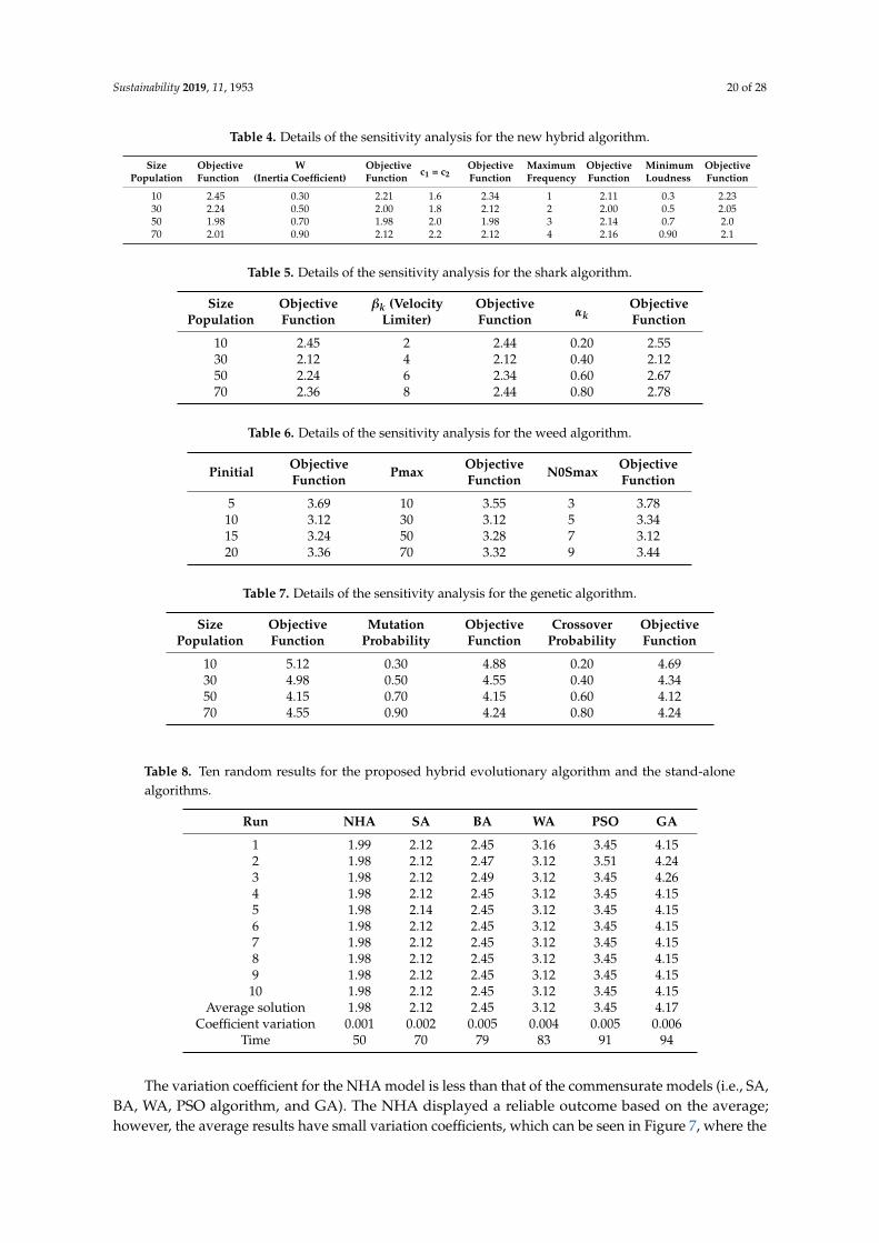
Tables 4–7 show the details of the sensitivity analysis for the proposed and comparableevolutionary algorithms. The sensitivity analysis shows the accuracy values of the random parametersobtained based on the variation in the value of the objective function versus the variation in the valuesof the random parameters. The size of the population for the NHA is 50 because the objective functionhas the smallest value (1.98). The maximum frequency for the NHA is 7 Hz, while the minimumfrequency is 2 Hz. The acceleration coefficients (c1 = c2) are equal to 2, and the inertia weight is 0.7.Other accurate values for the other algorithms can be seen in Tables 5–8. The population size for theSA is 30, and the velocity limit for this method is 4. The mutation and crossover probabilities are0.70 and 0.60, respectively. The size populations for Pinitial and Pmax based on the WA are 10 and 30,respectively. Additionally, other parameters can be seen in Tables 5–7.

Sustainability 2019, 11, 1953 19 of 28

5.3. Ten Random Results for Evolutionary Algorithms

Table 8 shows the ten random run results for different algorithms for the same year. The averagesolution attained using the NHA is 1.98, which is the lowest value among the other algorithms.The average solutions for the SA, BA, WA, PSO algorithm, and GA are 2.12, 2.45, 3.12, 3.45, and 4.15,respectively. On the basis of the achieved results, the NHA minimized the objective function betterthan the other algorithms. The computational time for the NHA is 50 s, whereas it is 70, 79, 83, 91,and 94 s for the SA, WA, BA, PSO algorithm, and GA, respectively. Accordingly, compared with theSA, BA, WA, PSO algorithm, and GA, the NHA decreased the computation time by 28%, 36%, 39%,82%, and 88%, respectively, which is an excellent enhancement result.

Table 3. Experimental results using benchmark functions. SD—standard deviation; ME—mean error;ANFE—average number of function evaluations; SR—success rate; NHA—new hybrid algorithm.

Function Algorithms SD ME ANFE SR

f1

Differential Evolution Algorithm 1.42 × 10−4 [52] 8.68 × 10−4 [52] 27,378 [52] 100Artificial Bee Colony Algorithm 2.02 × 10−4 [52] 7.54 × 10−4 [52] 35,091 [52] 100

Particle Swarm Optimization 6.72 × 10−5 9.34 × 10−4 45,914.5 100Bat Algorithm 5.12 × 10−5 6.12 × 10−4 231,245 100

Shark Algorithm 5.01 × 10−5 5.25 × 10−4 209,878 100Genetic Algorithm 1.34 × 10−5 9.56 × 10−4 37,094 100

Spider Monkey Algorithm 2.12 × 10−6 [52] 5.65 × 10−5 19,878 [52] 100Krill Algorithm 2.22 × 10−6 [52] 7.12 × 10−5 18,235 [52] 100

NHA 5.25 × 10−7 8.12 × 10−6 14,224 100

f2

Differential Evolution Algorithm 4.93 [52] 2.09 × 10−3 [53] 200,000 [52] 98Artificial Bee Colony Algorithm 3.14 × 10−4 [52] 7.48 × 10−4 [53] 87,039 [52] 98

Particle Swarm Optimization 1.35 × 10+1 2.98 × 10−3 200,000 98Bat Algorithm 3.24 × 10−5 3.12 × 10−5 54,223 98

Shark Algorithm 4.56 × 10−7 4.12 × 10−6 45,221 98Genetic Algorithm 8.78 2.12 × 10−3 205,000 98

Spider Monkey Algorithm 6.12 × 10−8 [53] 5.12 × 10−7 [53] 32,124 [53] 98Krill Algorithm 7.91 × 10−7 [53] 6.12 × 10−7 [53] 35,125 [53] 100

NHA 9.12 × 10−9 7.12 × 10−8 310,191 100

f3

Differential Evolution Algorithm 1.12 × 10−3 4.09 × 10−1 2725.5 100Artificial Bee Colony Algorithm 5.25 × 10−3 4.09 × 10−1 2567 85

Particle Swarm Optimization 5.64 × 10−3 4.02 × 10−1 4979 85Bat Algorithm 4.12 × 10−4 3.12 × 10−2 1285 85

Shark Algorithm 5.12 × 10−5 3.22 × 10−2 1100 98Genetic Algorithm 1.12 × 10−2 4.12 × 10+1 1400 98

Spider Monkey Algorithm 5.78 × 10−5 2.12 × 10−4 987 98Krill Algorithm 5.45 × 10−3 3.12 × 10−5 765 98

NHA 1.14 × 10−6 1.12 × 10−6 654 100

f4

Differential Evolution Algorithm 1.12 × 10+2 2.19 × 10+1 180,000 84Artificial Bee Colony Algorithm 1.18 × 10+1 1.19 × 10+1 170,000 84

Particle Swarm Optimization 6.70 × 10+2 2.80 × 10−3 200,000 84Bat Algorithm 5.70 × 10−3 1.12 × 10−4 180,000 84

Shark Algorithm 4.71 × 10−3 5.45 × 10−5 160,000 84Genetic Algorithm 6.14 × 10+3 1.21 × 10−2 210,000 84

Spider Monkey Algorithm 1.45 × 10−4 3.12 × 10−5 180,000 84Krill Algorithm 1.23 × 10−5 4.21 × 10−5 165,000 84

NHA 2.12 × 10−6 2.12 × 10−7 140,000 98

f5

Differential Evolution Algorithm 1.31 × 10−6 4.90 × 10−1 2741 100Artificial Bee Colony Algorithm 2.00 × 10−6 4.87 × 10−1 4811 100

Particle Swarm Optimization 6.12 × 10−7 4.75 × 10−1 4912 100Bat Algorithm 2.12 × 10−8 2.22 × 10−3 1811 100

Shark Algorithm 1.11 × 10−8 2.12 × 10−4 1712 100Genetic Algorithm 1.21 × 10−5 3.21 × 10−4 5121 100

Spider Monkey Algorithm 2.12 × 10−8 5.12 × 10−3 1001 100Krill Algorithm 1.14 × 10−8 5.45 × 10−4 987 100

NHA 1.41 × 10−9 6.78 × 10−5 567 100

Sustainability 2019, 11, 1953 20 of 28

Table 4. Details of the sensitivity analysis for the new hybrid algorithm.

SizePopulation

ObjectiveFunction

W(Inertia Coefficient)

ObjectiveFunction c1 = c2

ObjectiveFunction

MaximumFrequency

ObjectiveFunction

MinimumLoudness

ObjectiveFunction

10 2.45 0.30 2.21 1.6 2.34 1 2.11 0.3 2.2330 2.24 0.50 2.00 1.8 2.12 2 2.00 0.5 2.0550 1.98 0.70 1.98 2.0 1.98 3 2.14 0.7 2.070 2.01 0.90 2.12 2.2 2.12 4 2.16 0.90 2.1

Table 5. Details of the sensitivity analysis for the shark algorithm.

SizePopulation

ObjectiveFunction

βk (VelocityLimiter)

ObjectiveFunction αk

ObjectiveFunction

10 2.45 2 2.44 0.20 2.5530 2.12 4 2.12 0.40 2.1250 2.24 6 2.34 0.60 2.6770 2.36 8 2.44 0.80 2.78

Table 6. Details of the sensitivity analysis for the weed algorithm.

Pinitial ObjectiveFunction Pmax Objective

Function N0Smax ObjectiveFunction

5 3.69 10 3.55 3 3.7810 3.12 30 3.12 5 3.3415 3.24 50 3.28 7 3.1220 3.36 70 3.32 9 3.44

Table 7. Details of the sensitivity analysis for the genetic algorithm.

SizePopulation

ObjectiveFunction

MutationProbability

ObjectiveFunction

CrossoverProbability

ObjectiveFunction

10 5.12 0.30 4.88 0.20 4.6930 4.98 0.50 4.55 0.40 4.3450 4.15 0.70 4.15 0.60 4.1270 4.55 0.90 4.24 0.80 4.24

Table 8. Ten random results for the proposed hybrid evolutionary algorithm and the stand-alonealgorithms.

Run NHA SA BA WA PSO GA

1 1.99 2.12 2.45 3.16 3.45 4.152 1.98 2.12 2.47 3.12 3.51 4.243 1.98 2.12 2.49 3.12 3.45 4.264 1.98 2.12 2.45 3.12 3.45 4.155 1.98 2.14 2.45 3.12 3.45 4.156 1.98 2.12 2.45 3.12 3.45 4.157 1.98 2.12 2.45 3.12 3.45 4.158 1.98 2.12 2.45 3.12 3.45 4.159 1.98 2.12 2.45 3.12 3.45 4.1510 1.98 2.12 2.45 3.12 3.45 4.15

Average solution 1.98 2.12 2.45 3.12 3.45 4.17Coefficient variation 0.001 0.002 0.005 0.004 0.005 0.006

Time 50 70 79 83 91 94

The variation coefficient for the NHA model is less than that of the commensurate models (i.e., SA,BA, WA, PSO algorithm, and GA). The NHA displayed a reliable outcome based on the average;however, the average results have small variation coefficients, which can be seen in Figure 7, where the

Sustainability 2019, 11, 1953 21 of 28

average, minimum, and maximum solutions overlap with each other and are well matched. Figure 8shows the value of the objective function belonging to all data-intelligence models versus the numberof function evaluations (NFEs). The NFE for the NHA model is equal to 5000. The other establishedmodels have NFE values of 8000, 1000, 12,000, 14,000, and 15,000 (SA, BA, WA, GA, and PSO algorithm,respectively). Thus, the NHA can obtain the best solutions with a smaller NFE, which shows that theNHA can obtain the converged solution faster than other algorithms.

Sustainability 2019, 11, x FOR PEER REVIEW 20 of 29

Table 5. Details of the sensitivity analysis for the shark algorithm.

Size Population

Objective Function

kβ (Velocity Limiter)

Objective Function kα

Objective Function

10 2.45 2 2.44 0.20 2.55 30 2.12 4 2.12 0.40 2.12 50 2.24 6 2.34 0.60 2.67 70 2.36 8 2.44 0.80 2.78

Table 6. Details of the sensitivity analysis for the weed algorithm.

Pinitial Objective Function Pmax Objective Function N0Smax Objective Function 5 3.69 10 3.55 3 3.78

10 3.12 30 3.12 5 3.34 15 3.24 50 3.28 7 3.12 20 3.36 70 3.32 9 3.44

Table 7. Details of the sensitivity analysis for the genetic algorithm.

Size Population

Objective Function

Mutation Probability

Objective Function

Crossover Probability

Objective Function

10 5.12 0.30 4.88 0.20 4.69 30 4.98 0.50 4.55 0.40 4.34 50 4.15 0.70 4.15 0.60 4.12 70 4.55 0.90 4.24 0.80 4.24

The variation coefficient for the NHA model is less than that of the commensurate models (i.e., SA, BA, WA, PSO algorithm, and GA). The NHA displayed a reliable outcome based on the average; however, the average results have small variation coefficients, which can be seen in Figure 7, where the average, minimum, and maximum solutions overlap with each other and are well matched. Figure 8 shows the value of the objective function belonging to all data-intelligence models versus the number of function evaluations (NFEs). The NFE for the NHA model is equal to 5000. The other established models have NFE values of 8000, 1000, 12,000, 14,000, and 15,000 (SA, BA, WA, GA, and PSO algorithm, respectively). Thus, the NHA can obtain the best solutions with a smaller NFE, which shows that the NHA can obtain the converged solution faster than other algorithms.

Figure 7. Convergence curve for the maximum, minimum, and average solution.

0.9

1.1

1.3

1.5

1.7

1.9

2.1

0 1000 2000 3000 4000 5000 6000

Obj

ectiv

e Fu

nctio

n

Number of Function Evaluation

Max

Average

Min

Figure 7. Convergence curve for the maximum, minimum, and average solution.Sustainability 2019, 11, x FOR PEER REVIEW 21 of 29

Figure 8. Comparison of the fitness value and number of function evaluation (NFE) for different algorithms. GA—genetic algorithm.

Table 8. Ten random results for the proposed hybrid evolutionary algorithm and the stand-alone algorithms.

Run NHA SA BA WA PSO GA 1 1.99 2.12 2.45 3.16 3.45 4.15 2 1.98 2.12 2.47 3.12 3.51 4.24 3 1.98 2.12 2.49 3.12 3.45 4.26 4 1.98 2.12 2.45 3.12 3.45 4.15 5 1.98 2.14 2.45 3.12 3.45 4.15 6 1.98 2.12 2.45 3.12 3.45 4.15 7 1.98 2.12 2.45 3.12 3.45 4.15 8 1.98 2.12 2.45 3.12 3.45 4.15 9 1.98 2.12 2.45 3.12 3.45 4.15

10 1.98 2.12 2.45 3.12 3.45 4.15 Average solution 1.98 2.12 2.45 3.12 3.45 4.17

Coefficient variation 0.001 0.002 0.005 0.004 0.005 0.006 Time 50 70 79 83 91 94

5.4. Computed Irrigation Deficiencies

Different indexes were used to evaluate the irrigation deficiencies tabulated in Table 9. The highest correlation attained for the proposed model had a magnitude of 0.93. Additionally, the absolute error metric values (e.g., the mean absolute error (MAE) and root mean square error (RMSE)) prove that released water can supply the irrigation demand for the left and right canals based on a smaller error index value and greater correlation value. The SA attained an accurate level of modelling after the use of the proposed hybrid model. Figure 9 shows the mode of the irrigation supply for all applied algorithms. The average demand for the total operation period is 142.14 (106

m3), and the average amounts of released water for the NHA, SA, BA, WA, PSO algorithm and GA are 141.25, 140.33, 138.75, 135.43, 134.12 and 133.21 (106 m3), respectively. Thus, the NHA can supply the irrigation demand as a primary priority in this problem. The volumetric reliability, vulnerability and resiliency indexes were used for more detailed information and a deep comparative analysis of all implemented algorithms. The high percentage for the volumetric reliability index found for the NHA showed that irrigation demands can be supplied for more operation periods; therefore, the volume of released water can respond to downstream irrigation demands. In fact, the volumetric reliability index based on the NHA is 5%, 8%, 17%, 18% and 31% greater than that based on the SA, BA, WA, PSO algorithm and GA, respectively.

0

2000

4000

6000

8000

10000

12000

14000

16000

NHA SA BA WA SA GA

NFE

Method

Figure 8. Comparison of the fitness value and number of function evaluation (NFE) for differentalgorithms. GA—genetic algorithm.

5.4. Computed Irrigation Deficiencies

Different indexes were used to evaluate the irrigation deficiencies tabulated in Table 9. The highestcorrelation attained for the proposed model had a magnitude of 0.93. Additionally, the absolute errormetric values (e.g., the mean absolute error (MAE) and root mean square error (RMSE)) prove thatreleased water can supply the irrigation demand for the left and right canals based on a smaller errorindex value and greater correlation value. The SA attained an accurate level of modelling after theuse of the proposed hybrid model. Figure 9 shows the mode of the irrigation supply for all appliedalgorithms. The average demand for the total operation period is 142.14 (106 m3), and the averageamounts of released water for the NHA, SA, BA, WA, PSO algorithm and GA are 141.25, 140.33, 138.75,135.43, 134.12 and 133.21 (106 m3), respectively. Thus, the NHA can supply the irrigation demand as aprimary priority in this problem. The volumetric reliability, vulnerability and resiliency indexes wereused for more detailed information and a deep comparative analysis of all implemented algorithms.The high percentage for the volumetric reliability index found for the NHA showed that irrigationdemands can be supplied for more operation periods; therefore, the volume of released water can

Sustainability 2019, 11, 1953 22 of 28

respond to downstream irrigation demands. In fact, the volumetric reliability index based on theNHA is 5%, 8%, 17%, 18% and 31% greater than that based on the SA, BA, WA, PSO algorithm andGA, respectively.

Table 9. Evaluation of different algorithms for irrigation demands based on differentindexes. NHA—new hybrid algorithm; SA—shark algorithm; BA—bat algorithm; WA—weedalgorithm; PSO—particle swarm optimization; GA—genetic algorithm; MOGA—multi-objective GA;MOPSO—multi-objective PSO.

Index Equation NHA SA BA WA PSO GA MOGA MOPSO

Correlation Coefficient r =

T∑

t=1(Dt−Dt).(Rt−Rt)√

T∑

t=1(Dt−Dt)

2.

T∑

t=1(Rt−Rt)

0.93 0.91 0.86 0.87 0.75 0.67 0.74 0.83

Root Mean Square Error (RMSE)(106 m3) RMSE =

√T∑

t=1(Dt−Rt)

2

T5.1 7.2 8.8 9.3 10.5 11.8 9.6 8.7

Mean absolute Error(106 m3) MAE =

T∑

t=1|Dt−Rt |

T4.3 5.59 6.1 7.1 6.9 6.4 6.3 6.1

Volumetric Reliability Index% αV =

T∑

t=1Rt

T∑

t=1Dt

× 100 95% 90% 87% 78% 75% 64% 77% 79%

Resiliency Index% γi =fsiFi

45% 40% 38% 35% 33% 29% 35% 34%

Vulnerability Index λ = MaxTt=1

(Dt−Rt

Dt

)× 100 14% 20% 21% 23% 24% 25% 22% 21%

Dt: demand; Dt: average demand; Rt: released water; and Rt: average released water.

Sustainability 2019, 11, x FOR PEER REVIEW 23 of 29

Figure 9. (a) Released water for downstream irrigation and (b) power production for downstream demand.

Additionally, Reddy and Kumar [53] optimized this system based on the multi-objective GA (MOGA) and multi-objective PSO (MOPSO) algorithms. These multi-objective algorithms can be considered substitution strategies instead of weighting methods, and the structure and preparation of such algorithms are complex. The results indicated that the NHA has a better performance than the MOGA and the MOPSO algorithm; therefore, the volumetric reliability index for the NHA is greater than that for the MOGA and the MOPSO algorithms. For example, the Pareto fronts are shown in Figure 10. The marginal rate of substitution strategy [54] is used to select the best solution. The marginal rate of substitution can be calculated based on sacrificing certain terms of the objective function to improve the value of the other terms of the objective function. When one solution has the maximum value of marginal rate of substitution, it is the most suitable solution; in other words, the best solution has the highest slope for two objective functions in the Pareto front. When the MOGA and the MOPSO algorithm are used, a large number of solutions can be observed; thus, the problem must be simplified. Therefore, a simple clustering strategy is used to filter 200 solutions to 20 solutions. First, there are N clusters, and the cluster ranges are calculated for all pairs of clusters; then, each two clusters with the minimum range are combined to generate the large cluster. Finally, the solutions with the minimum average distance from other solutions in the cluster are considered as alternative solutions for clustering (Figure 10). The determined point blue is the optimal solution.

0

50

100

150

200

250

0 10 20 30 40 50 60 70 80 90 100

Rel

ease

d W

ater

(10^

6 m

3)

Month

Demand NHA SA

BA WA PSO

GA

(a)

0

5

10

15

20

25

30

0 10 20 30 40 50 60 70 80 90 100

Pow

er P

rodu

ctio

n (1

0^6

kwh)

Month

Demand NHA

SA BA

WA PSO

GA

(b)

Figure 9. (a) Released water for downstream irrigation and (b) power production for downstreamdemand.

Sustainability 2019, 11, 1953 23 of 28

Additionally, Reddy and Kumar [53] optimized this system based on the multi-objective GA(MOGA) and multi-objective PSO (MOPSO) algorithms. These multi-objective algorithms can beconsidered substitution strategies instead of weighting methods, and the structure and preparationof such algorithms are complex. The results indicated that the NHA has a better performance thanthe MOGA and the MOPSO algorithm; therefore, the volumetric reliability index for the NHA isgreater than that for the MOGA and the MOPSO algorithms. For example, the Pareto fronts areshown in Figure 10. The marginal rate of substitution strategy [54] is used to select the best solution.The marginal rate of substitution can be calculated based on sacrificing certain terms of the objectivefunction to improve the value of the other terms of the objective function. When one solution hasthe maximum value of marginal rate of substitution, it is the most suitable solution; in other words,the best solution has the highest slope for two objective functions in the Pareto front. When the MOGAand the MOPSO algorithm are used, a large number of solutions can be observed; thus, the problemmust be simplified. Therefore, a simple clustering strategy is used to filter 200 solutions to 20 solutions.First, there are N clusters, and the cluster ranges are calculated for all pairs of clusters; then, each twoclusters with the minimum range are combined to generate the large cluster. Finally, the solutionswith the minimum average distance from other solutions in the cluster are considered as alternativesolutions for clustering (Figure 10). The determined point blue is the optimal solution.Sustainability 2019, 11, x FOR PEER REVIEW 24 of 29

Figure 10. Pareto front for the algorithms. MOGA—multi-objective GA; MOPSO—multi-objective PSO.

The vulnerability index for the NHA was 12%, which was the lowest percentage among the analyzed methods. The maximum intensity of the failure probability occurred with the NHA and was less than that of other evolutionary algorithms. The greatest value of the vulnerability index was related to the GA. Additionally, the NHA had a better performance than the MOGA and the MOPSO algorithms based on the lower value of the vulnerability index.

Finally, the resiliency index of the NHA was 45%, which was the highest percentage among the analysed methods; therefore, the multi-purpose system can escape more quickly from critical periods, such as drought periods.

Figure 11 shows that the NHA has the smallest average annual deficit among the evaluated methods. The average annual deficit for the NHA is 10%, 12%, 15%, 17%, and 18% less than that for the SA, BA, WA, PSO algorithm, and GA, respectively. The historical water demand required for various uses was recorded during an earlier time period, whereas the released water decision pattern was calculated based on the achieved optimal operation rules from each algorithm based on objective functions. Finally, a comparative analysis was carried out to identify the gap between the water demand for the irrigation requirement and power production and the allocated water release. The released water as a decision variable was calculated, and then the power generation was calculated based on released water; the resulting power produced was 106 kWh, which was then compared with the actual power required for downstream demands.

Figure 11. Average annual deficits for different algorithms.

020406080

100120140160180200

10000 12000 14000 16000 18000 20000

f (2)

: Hyd

ropo

wer

gen

erat

ed

(Mkw

h)

f(1): Sum of squared irrigation deficits (Mm3)

MOPSO

MOGA

Optimal Solution

0

0.5

1

1.5

2

2.5

1 2 3 4 5 6 7 8 9 10

Aver

age

annu

al d

efici

t (M

CM)

Year

NHA

SA

BA

WA

PSO

GA

Figure 10. Pareto front for the algorithms. MOGA—multi-objective GA; MOPSO—multi-objective PSO.

The vulnerability index for the NHA was 12%, which was the lowest percentage among theanalyzed methods. The maximum intensity of the failure probability occurred with the NHA andwas less than that of other evolutionary algorithms. The greatest value of the vulnerability index wasrelated to the GA. Additionally, the NHA had a better performance than the MOGA and the MOPSOalgorithms based on the lower value of the vulnerability index.

Finally, the resiliency index of the NHA was 45%, which was the highest percentage among theanalysed methods; therefore, the multi-purpose system can escape more quickly from critical periods,such as drought periods.

Figure 11 shows that the NHA has the smallest average annual deficit among the evaluatedmethods. The average annual deficit for the NHA is 10%, 12%, 15%, 17%, and 18% less than thatfor the SA, BA, WA, PSO algorithm, and GA, respectively. The historical water demand requiredfor various uses was recorded during an earlier time period, whereas the released water decisionpattern was calculated based on the achieved optimal operation rules from each algorithm based onobjective functions. Finally, a comparative analysis was carried out to identify the gap between thewater demand for the irrigation requirement and power production and the allocated water release.The released water as a decision variable was calculated, and then the power generation was calculated

Sustainability 2019, 11, 1953 24 of 28

based on released water; the resulting power produced was 106 kWh, which was then compared withthe actual power required for downstream demands.

Sustainability 2019, 11, x FOR PEER REVIEW 24 of 29

Figure 10. Pareto front for the algorithms. MOGA—multi-objective GA; MOPSO—multi-objective PSO.

The vulnerability index for the NHA was 12%, which was the lowest percentage among the analyzed methods. The maximum intensity of the failure probability occurred with the NHA and was less than that of other evolutionary algorithms. The greatest value of the vulnerability index was related to the GA. Additionally, the NHA had a better performance than the MOGA and the MOPSO algorithms based on the lower value of the vulnerability index.

Finally, the resiliency index of the NHA was 45%, which was the highest percentage among the analysed methods; therefore, the multi-purpose system can escape more quickly from critical periods, such as drought periods.

Figure 11 shows that the NHA has the smallest average annual deficit among the evaluated methods. The average annual deficit for the NHA is 10%, 12%, 15%, 17%, and 18% less than that for the SA, BA, WA, PSO algorithm, and GA, respectively. The historical water demand required for various uses was recorded during an earlier time period, whereas the released water decision pattern was calculated based on the achieved optimal operation rules from each algorithm based on objective functions. Finally, a comparative analysis was carried out to identify the gap between the water demand for the irrigation requirement and power production and the allocated water release. The released water as a decision variable was calculated, and then the power generation was calculated based on released water; the resulting power produced was 106 kWh, which was then compared with the actual power required for downstream demands.

Figure 11. Average annual deficits for different algorithms.

020406080

100120140160180200

10000 12000 14000 16000 18000 20000

f (2)

: Hyd

ropo

wer

gen

erat

ed

(Mkw

h)

f(1): Sum of squared irrigation deficits (Mm3)

MOPSO

MOGA

Optimal Solution

0

0.5

1

1.5

2

2.5

1 2 3 4 5 6 7 8 9 10

Aver

age

annu

al d

efici

t (M

CM)

Year

NHA

SA

BA

WA

PSO

GA

Figure 11. Average annual deficits for different algorithms.

5.5. Computational Power Production

The downstream demand for power is 18.90 (106 kwh), and the average amount of producedpower based on the NHA is 18.08 (106 kwh), while it is 17.99, 17.32, 16.96, 16.32, and 15.34 (106 kwh)for the SA, BA, WA, PSO algorithm, and GA, respectively (see Figure 6b). Thus, the NHA can producemore power to supply the demand (Table 10). Additionally, the correlation coefficient for the NHAis greater than that for other algorithms, and the root mean square error (RMSE) and mean absoluteerror (MAE) have the smallest values in the NHA among the evaluated algorithms based on thedifference between demand and power production. Additionally, the NHA has a better performancethan the MOGA and the MOPSO algorithms based on the lower values for the error indexes andhigher correlation values.

Thus, the NHA can supply the irrigation demand first; then, the power production can be usedafter the irrigation supply. Additionally, although the release of more water may generate more power,a considerable deficiency in irrigation would result. Thus, more weight is assigned to the irrigationobjective function to ensure that the demand for irrigation is met; ensuring the necessary powerproduction is an additional concern for policymakers.

Table 10. Evaluation of different algorithms for irrigation demands based on different indexes.

Index Equation NHA SA BA WA PSO GA MOGA(Reddy, 2006)

MOPSO(Reddy, 2006)

Correlation Coefficient r =

T∑

t=1(Pdt−Pdt).(Pst−Pst)√

T∑

t=1(Pdt−Pobt)

2.

T∑

t=1(Pst−Pst)

93% 90% 87% 75% 69% 65% 73% 75%

Root Mean Square Error(RMSE)

(106 kwh) RMSE =

√T∑

t=1(Pobt−Pst)

2

T3.1 4.9 4.2 3.8 4.2 3.7 3.5 3.8

Mean Absolute Error(MAE)

(106 kwh) MAE =

T∑

t=1|Pobt−Pst |

T3.2 4.1 3.8 3.6 3.4 3.5 3.3 3.4

Pdt: power demand; Pdt: average power demand; and Pst: simulated produced power by algorithms.

6. Conclusions

The current research is dedicated to the implementation of a new hybrid intelligence model basedon integrating two meta-heuristic algorithms for optimizing the operation of a multi-purpose reservoirwater system. The optimization problem is solved to satisfy irrigation demands and hydropowerproduction for one case study in India. The capability of the BA is improved by hybridization with the

Sustainability 2019, 11, 1953 25 of 28

PSO algorithm based on local and global search strategies and the substitution of weaker solutions ineach algorithm with the best solutions of the other algorithms. The main idea behind the procedure ofthe proposed NHA is to avoid the possible worst solutions using the BA and the resulting decline inlocal optima; in addition, the NHA enhanced the convergence rate using the PSO algorithm.

After applying the proposed NHA for a multi-purpose reservoir water system, namely the BhadraDam in India, it could be concluded that the NHA could provide a satisfactory improvement todecreasing irrigation deficiencies. In quantitative terms, the average irrigation demand was 142.14(106 m3), and the NHA can release 141.25 (106 m3), which represents a much higher level of accuracyover comparable models. The average demand for power production is 18.08 (106 kwh), and theproduced power using the NHA is 17.99 (106 kwh), which represents the capability of the NHA forapplied applications.

It can be concluded that the proposed NHA as an intelligent model could contribute to providingreliable solutions for complex multi-purpose reservoir systems to optimize the operation rule forsimilar reservoir systems worldwide. In addition, the NHA could be integrated with other forecastingmodels for additional reservoir hydrological variables to optimize its operation under different climatechange scenarios in future periods. Furthermore, the NHA could be used for multi-purpose reservoirsystems and other multi-purpose engineering optimization applications.

Although the proposed NHA showed superior performance over the other optimizationalgorithms, it still experienced a challenge during initialization because several random parametersmust be initialized. This step may prolong the computational time for convergence. In addition tothe need to initialize the random parameters for the BA and PSO algorithms within the definition ofthe NHA communication, a simultaneous procedure must also be adopted to update these randomparameters within the simulation model of the reservoir, and such requirements should be consideredwhen applying the NHA to other case studies.

Author Contributions: Formal analysis: Z.M.Y., M.E., L.S.H., and A.E.-S.; Methodology: M.E.; Resources: M.S.H.;Supervision: A.E.-S.; Validation, N.Z. and A.N.A.; Visualization: N.S.M., W.Z.B.J., and A.N.A.; Writing—originaldraft: S.B.K. and H.A.A.; Writing—review & editing: C.M.F.

Acknowledgments: The authors greatly appreciate the financial support received from the Ministry of Education(MOE) research grant Fundamental Research Grant Scheme (FRGS) 20180120FRGS and University of MalayaResearch Grant (UMRG) coded RP025A-18SUS, University of Malaya, Malaysia. In addition, this studywas partially funded by the TNB Seeding Fund, Institute of Power Energy (IPE) and Institute of EnergyInfrastructure (IEI), Universiti Tenaga Nasional, Malaysia, through research grants coded U-TG-CR-18-03 andU-TG-RD-17-06, respectively.

Conflicts of Interest: The authors declare no conflict of interest. The funders had no role in the design of thestudy; in the collection, analyses, or interpretation of data; in the writing of the manuscript, and in the decision topublish the results.

References

1. Pedro-Monzonís, M.; Solera, A.; Ferrer, J.; Estrela, T.; Paredes-Arquiola, J. A review of water scarcity anddrought indexes in water resources planning and management. J. Hydrol. 2015, 527, 482–493. [CrossRef]

2. You, J.Y.; Cai, X. Hedging rule for reservoir operations: 2. A numerical model. Water Resour. Res. 2008, 44.[CrossRef]

3. Fang, H.; Hu, T.; Zeng, X.; Wu, F. Simulation-optimization model of reservoir operation based on targetstorage curves. Water Sci. Eng. 2014, 7, 433–445. [CrossRef]

4. Srinivasan, K.; Kumar, K. Multi-Objective Simulation-Optimization Model for Long-term ReservoirOperation using Piecewise Linear Hedging Rule. Water Resour. Manag. 2018, 32, 1901–1911. [CrossRef]

5. Xie, A.; Liu, P.; Guo, S.; Zhang, X.; Jiang, H.; Yang, G. Optimal Design of Seasonal Flood Limited Water Levelsby Jointing Operation of the Reservoir and Floodplains. Water Resour. Manag. 2017, 32, 179–193. [CrossRef]

6. Adeyemo, J.A. Reservoir operation using multi-objective evolutionary algorithms—A review. Asian J. Sci.Res. 2011, 4, 16–27. [CrossRef]

Sustainability 2019, 11, 1953 26 of 28

7. Karamouz, M.; Nazif, S.; Sherafat, M.A.; Zahmatkesh, Z. Development of an Optimal Reservoir OperationScheme Using Extended Evolutionary Computing Algorithms Based on Conflict Resolution Approach:A Case Study. Water Resour. Manag. 2014, 28, 3539–3554. [CrossRef]

8. Azizipour, M.; Ghalenoei, V.; Afshar, M.H.; Solis, S.S. Optimal Operation of Hydropower Reservoir SystemsUsing Weed Optimization Algorithm. Water Resour. Manag. 2016, 30, 3995–4009. [CrossRef]

9. Han, C.; Zheng, B.; Qin, Y.; Ma, Y.; Yang, C.; Liu, Z.; Cao, W.; Chi, M. Impact of upstream river inputsand reservoir operation on phosphorus fractions in water-particulate phases in the Three Gorges Reservoir.Sci. Total Environ. 2018, 610–611, 1546–1556. [CrossRef]

10. Wan, W.; Guo, X.; Lei, X.; Jiang, Y.; Wang, H. A Novel Optimization Method for Multi-Reservoir OperationPolicy Derivation in Complex Inter-Basin Water Transfer System. Water Resour. Manag. 2017, 32, 31–51.[CrossRef]

11. Moeini, R.; Babaei, M. Constrained improved particle swarm optimization algorithm for optimal operationof large scale reservoir: Proposing three approaches. Evol. Syst. 2017, 8, 287–301. [CrossRef]

12. Zyoud, S.H.; Kaufmann, L.G.; Shaheen, H.; Samhan, S.; Fuchs-Hanusch, D. A framework for water lossmanagement in developing countries under fuzzy environment: Integration of Fuzzy AHP with FuzzyTOPSIS. Expert Syst. Appl. 2016, 61, 86–105. [CrossRef]

13. Rabiei, M.; Aalami, M.; Talatahari, S. Reservoir Operation Optimization using CBO, ECBO and vpsalgorithms. Iran Univ. Sci. Technol. 2018, 8, 489–509.

14. Tayfur, G. Modern Optimization Methods in Water Resources Planning, Engineering and Management.Water Resour. Manag. 2017, 31, 3205–3233. [CrossRef]

15. Bennett, C.; Stewart, R.A.; Beal, C.D. ANN-based residential water end-use demand forecasting model.Expert Syst. Appl. 2013, 40, 1014–1023. [CrossRef]

16. Nabaei, A.; Hamian, M.; Parsaei, M.R.; Safdari, R.; Samad-Soltani, T.; Zarrabi, H.; Ghassemi, A. Topologiesand performance of intelligent algorithms: A comprehensive review. Artif. Intell. Rev. 2016. [CrossRef]

17. Ethteram, M.; Mousavi, S.F.; Karami, H.; Farzin, S.; Deo, R.; Othman, F.B.; Chau, K.; Sarkamaryan, S.;Singh, V.P.; El-Shafie, A. Bat algorithm for dam–reservoir operation. Environ. Earth Sci. 2018, 77, 510.[CrossRef]

18. Ehteram, M.; Singh, V.; Karami, H.; Hosseini, K.; Dianatikhah, M.; Hossain, M.; Ming Fai, C.; El-Shafie, A.Irrigation Management Based on Reservoir Operation with an Improved Weed Algorithm. Water 2018, 10,1267. [CrossRef]

19. Allawi, M.F.; Jaafar, O.; Mohamad Hamzah, F.; Ehteram, M.; Hossain, M.S.; El-Shafie, A. Operating areservoir system based on the shark machine learning algorithm. Environ. Earth Sci. 2018, 77, 366. [CrossRef]

20. Allawi, M.F.; Jaafar, O.; Mohamad Hamzah, F.; Koting, S.B.; Mohd, N.S.B.; El-Shafie, A. Forecastinghydrological parameters for reservoir system utilizing artificial intelligent models and exploring theirinfluence on operation performance. Knowl.-Based Syst. 2019, 163, 907–926. [CrossRef]

21. Raso, L.; Chiavico, M.; Dorchies, D. Optimal and Centralized Reservoir Management for Drought and FloodProtection on the Upper Seine–Aube River System Using Stochastic Dual Dynamic Programming. J. WaterResour. Plan. Manag. 2019, 145, 5019002. [CrossRef]

22. Allawi, M.F.; Jaafar, O.; Ehteram, M.; Mohamad Hamzah, F.; El-Shafie, A. Synchronizing Artificial IntelligenceModels for Operating the Dam and Reservoir System. Water Resour. Manag. 2018, 32, 3373–3389. [CrossRef]

23. Ehteram, M.; Karami, H.; Farzin, S. Reservoir Optimization for Energy Production Using a New EvolutionaryAlgorithm Based on Multi-Criteria Decision-Making Models. Water Resour. Manag. 2018, 32, 2539–2560.[CrossRef]

24. Ehteram, M.; Mousavi, S.F.; Karami, H.; Farzin, S.; Emami, M.; Binti Othman, F.; Amini, Z.; Kisi, O.;El-Shafie, A. Fast convergence optimization model for single and multi-purposes reservoirs using hybridalgorithm. Adv. Eng. Inform. 2017, 32, 287–298. [CrossRef]

25. Afshar, A.; Shafii, M.; Haddad, O.B. Optimizing multi-reservoir operation rules: An improved HBMOapproach. J. Hydroinform. 2010, 13, 121. [CrossRef]

26. Fallah-Mehdipour, E.; Bozorg Haddad, O.; Mariño, M.A. Real-Time Operation of Reservoir System byGenetic Programming. Water Resour. Manag. 2012, 26, 4091–4103. [CrossRef]

27. Ostadrahimi, L.; Mariño, M.A.; Afshar, A. Multi-reservoir Operation Rules: Multi-swarm PSO-basedOptimization Approach. Water Resour. Manag. 2011, 26, 407–427. [CrossRef]

Sustainability 2019, 11, 1953 27 of 28

28. Bolouri-Yazdeli, Y.; Bozorg Haddad, O.; Fallah-Mehdipour, E.; Mariño, M.A. Evaluation of real-timeoperation rules in reservoir systems operation. Water Resour. Manag. 2014, 28, 715–729. [CrossRef]

29. Akbari-Alashti, H.; Bozorg Haddad, O.; Fallah-Mehdipour, E.; Mariño, M.A. Multi-reservoir real-timeoperation rules: A new genetic programming approach. Proc. Inst. Civ. Eng. Water Manag. 2014, 167, 561–576.[CrossRef]

30. Haddad, O.B.; Moravej, M.; Loáiciga, H.A. Application of the Water Cycle Algorithm to the OptimalOperation of Reservoir Systems. J. Irrig. Drain. Eng. 2015, 141, 04014064. [CrossRef]

31. Haddad, O.B.; Hosseini-Moghari, S.-M.; Loáiciga, H.A. Biogeography-Based Optimization Algorithm forOptimal Operation of Reservoir Systems. J. Water Resour. Plan. Manag. 2016, 142, 04015034. [CrossRef]

32. Zhang, Z.; Jiang, Y.; Zhang, S.; Geng, S.; Wang, H.; Sang, G. An adaptive particle swarm optimizationalgorithm for reservoir operation optimization. Appl. Soft Comput. J. 2014, 18, 167–177. [CrossRef]

33. Hosseini-Moghari, S.-M.; Morovati, R.; Moghadas, M.; Araghinejad, S. Optimum Operation of ReservoirUsing Two Evolutionary Algorithms: Imperialist Competitive Algorithm (ICA) and Cuckoo OptimizationAlgorithm (COA). Water Resour. Manag. 2015, 29, 3749–3769. [CrossRef]

34. Ehteram, M.; Karami, H.; Mousavi, S.-F.; Farzin, S.; Kisi, O. Evaluation of contemporary evolutionaryalgorithms for optimization in reservoir operation and water supply. J. Water Supply Res. Technol. 2017,jws2017109. [CrossRef]

35. Ehteram, M.; Karami, H.; Mousavi, S.-F.; Farzin, S.; Kisi, O. Optimization of energy management andconversion in the multi-reservoir systems based on evolutionary algorithms. J. Clean. Prod. 2017, 168,1132–1142. [CrossRef]

36. Garg, H. A hybrid GSA-GA algorithm for constrained optimization problems. Inf. Sci. 2019, 478, 499–523.[CrossRef]

37. Patwal, R.S.; Narang, N.; Garg, H. A novel TVAC-PSO based mutation strategies algorithm for generationscheduling of pumped storage hydrothermal system incorporating solar units. Energy 2018, 142, 822–837.[CrossRef]

38. Garg, H. A hybrid PSO-GA algorithm for constrained optimization problems. Appl. Math. Comput. 2016, 274,292–305. [CrossRef]

39. Garg, H. An efficient biogeography based optimization algorithm for solving reliability optimizationproblems. Swarm Evol. Comput. 2015, 24, 1–10. [CrossRef]

40. Shah, H.; Tairan, N.; Garg, H.; Ghazali, R. Global Gbest Guided-Artificial Bee Colony Algorithm forNumerical Function Optimization. Computers 2018, 7, 69. [CrossRef]

41. Yang, X.S. Bat algorithm for multi-objective optimisation. Int. J. Bio-Inspired Comput. 2011, 3, 267. [CrossRef]42. Gandomi, A.H.; Yang, X.S. Chaotic bat algorithm. J. Comput. Sci. 2014, 5, 224–232. [CrossRef]43. Yang, X.S. A new metaheuristic Bat-inspired Algorithm. In Studies in Computational Intelligence; Springer:

Berlin/Heidelberg, Germany, 2010; Volume 284, pp. 65–74.44. Bozorg-Haddad, O.; Karimirad, I.; Seifollahi-Aghmiuni, S.; Loáiciga, H.A. Development and Application of

the Bat Algorithm for Optimizing the Operation of Reservoir Systems. J. Water Resour. Plan. Manag. 2015,141, 04014097. [CrossRef]

45. Wang, Y.Y.; Zhou, J.; Zhou, C.; Wang, Y.Y.; Qin, H.; Lu, Y. An improved self-adaptive PSO technique forshort-term hydrothermal scheduling. Expert Syst. Appl. 2012, 39, 2288–2295. [CrossRef]

46. Karami, H.; Mousavi, S.F.; Farzin, S.; Ehteram, M.; Singh, V.P.; Kisi, O. Improved Krill Algorithm for ReservoirOperation. Water Resour. Manag. 2018, 32, 3353–3372. [CrossRef]

47. Li, L.; Zhou, Y. A novel complex-valued bat algorithm. Neural Comput. Appl. 2014, 25, 1369–1381. [CrossRef]48. Kennedy, J.; Eberhart, R. Particle swarm optimization. Neural Netw. 1995, 4, 1942–1948. [CrossRef]49. Ehteram, M.; Karami, H.; Farzin, S. Reducing Irrigation Deficiencies Based Optimizing Model for

Multi-Reservoir Systems Utilizing Spider Monkey Algorithm. Water Resour. Manag. 2018, 32, 2315–2334.[CrossRef]

50. Mehrabian, A.R.; Lucas, C. A novel numerical optimization algorithm inspired from weed colonization.Ecol. Inform. 2006, 1, 355–366. [CrossRef]

51. Hersovici, M.; Jacovi, M.; Maarek, Y.S.; Pelleg, D.; Shtalhaim, M.; Ur, S. The shark-search algorithm.An application: Tailored Web site mapping. Comput. Netw. ISDN Syst. 1998, 30, 317–326. [CrossRef]

52. Bansal, J.C.; Sharma, H.; Jadon, S.S.; Clerc, M. Spider Monkey Optimization algorithm for numericaloptimization. Memetic Comput. 2014, 6, 31–47. [CrossRef]

Sustainability 2019, 11, 1953 28 of 28

53. Reddy, M.J.; Kumar, D.N. Optimal reservoir operation using multi-objective evolutionary algorithm.Water Resour. Manag. 2006, 20, 861–878. [CrossRef]

54. Deb, K.; Zhu, L.; Kulkarni, S. Multi-scenario, multi-objective optimization using evolutionary algorithms:Initial results. In Proceedings of the 2015 IEEE Congress on Evolutionary Computation, Sendai, Japan,25–28 May 2015; pp. 1877–1884.

© 2019 by the authors. Licensee MDPI, Basel, Switzerland. This article is an open accessarticle distributed under the terms and conditions of the Creative Commons Attribution(CC BY) license (http://creativecommons.org/licenses/by/4.0/).