a novel methodology for digital removal of periodic noise ... · pdf fileusing the following...

Contemporary Engineering Sciences, Vol. 7, 2014, no. 3, 103 - 116 HIKARI Ltd, www.m-hikari.com

http://dx.doi.org/10.12988/ces.2014.31065

A Novel Methodology for Digital Removal of

Periodic Noise Using 2D Fast Fourier Transforms

Ashraf Abdel-Karim Helal Abu-Ein

Department of Computer Engineering, Faculty of Engineering Technology P.O. Box: 15008, Al Balqa Applied University, Amman, Jordan

[email protected]

Copyright © 2013 Ashraf Abdel-Karim Helal Abu-Ein. This is an open access article distributed under the Creative Commons Attribution License, which permits unrestricted use, distribution, and reproduction in any medium, provided the original work is properly cited.

Abstract An efficient methodology to remove periodic noise from digital images is proposed. The methodology steps is discussed, analyzed and implemented. Color image is to be converted to gray image, and then 2D fast Fourier transform (2DFFT) is to be applied on the gray image. The magnitude of applying 2DFFT is to be analyzed in order to get the periodic filter, which is to be correlated with the magnitude matrix, and the output of correlation is to be used with the angle matrix to get the un noisy gray image. Experimental results are shown and they demonstrate the efficiency of using that the proposed filter for removing high and low frequencies. Keywords: Color image, gray image, direct transform, indirect transform, periodic noise, 2DFFT, inverse Fourier transform, magnitude matrix, angle matrix

I. INTRODUCTION Color digital images play an important role in daily life application such as television, ultrasound imaging, magnetic resonance imaging, computer tomography as well as in areas of research and technology. Image acquisition is the process of obtaining a digitized image from a real world source. Each step in the acquisition process may introduce random changes into the values of pixels in the image. These changes are called noise [12, 13].

104 Ashraf Abdel-Karim Helal Abu-Ein Periodic (stationary) noise commonly caused by interference between electronic components and has a fixed amplitude [14, 15], frequency and phase as shown in figure (1).

Figure (1): Periodic noise

Periodic noise typically arises from interference during image acquisition. Spatially dependent noise type can be effectively reduced via frequency domain filtering Noise parameters can often be estimated by observing the Fourier spectrum of the image – Periodic noise tends to produce frequency spikes [16] as shown in figure (2).

Figure (2): Sample periodic images and their spectra

Many applications [1, 2, 3, 22, 23 and 24] of digital images processing require an estimation of the noise level that should be local in time and in frequency such that non-stationary and colored noise can be dealt with. Noise level estimation is usually done by explicit detection of time segments that contain only noise, or explicit estimation of harmonically related spectral components [1]. For a given narrow band, e.g. each frequency bin k, the noise distribution can be

modeled by means of Rayleigh with mode ( )kσ Once ( )kσ has been estimated for all k, the curve passing through these σ -value magnitudes defines a reference noise level Lσ . Using the following equation it is now possible to adjust the noise threshold to a desired percentage of misclassified noise peaks. [1-4]

1( ) 2 log(1 ), 0 1px F p p pσ−= = − − < < That is, the frequency dependent _ (k) can be calculated if the mean noise magnitude E[X], which is also frequency dependent, can be estimated [5, 6, and 7].

Novel methodology for digital removal of periodic noise 105 However, estimation of the expected noise magnitude corresponding to each frequency bin requires sufficient observations for statistical evaluation. Most of the existing approaches [1] rely on observations from neighboring frames. Our approach relies on the assumption that the noise spectral envelope is changing only weakly with the bin index k such that we may use the observed spectral peaks in the predefined subbands2 to estimate the (frequency dependent) mean noise level Lm by means of a smoothed curve over the noise peaks. Some parameters affect the procedure of noise estimation and calculating the estimated mean value of the noise and we will considerate the following parameters:

- No of standard deviations of noise to reject.[5,6] - No of filter scales to use. - Multiplying factor between scales. - No of orientations to use.[5] - Gray image size. - Ratio of angular interval between filter orientations and the standard

deviation of the angular Gaussian function used to construct filters in the freq. plane [7-11].

- Ratio of the standard deviation of the Gaussian describing the log Gabor filter's transfer function in the frequency domain to the filter center frequency [10, 11].

- II. Image filtration in the frequency domain

It was shown [17, 18] that 2D Fourier transform can be represented by equation 3.1

1 12 ( / / )

0 0( , ) ( , )

M Nj ux M vy N

x yF u v f x y e π

− −− +

= =

= ⋅∑ ∑(2.1)

Where f(x,y) is a digital image of size MxN. Equation 3.1. must be evaluated for values of the discrete variables u and v in the range u=0....M-1, v=0...N-1. Given the transform F (u,v) we can obtain f(x,y) by using the inverse discrete Fourier transform: 3.2 and

1 12 ( / / )

0 0

1( , ) ( , )M N

j ux M vy N

u vf x y T u v e

MNπ

− −+

= =

= ⋅∑ ∑(2.2)

The variables u and v represented in the equations 2.1 and 2.2 are frequency variables. The function T (u,v) is often called the frequency domain representation of f(x,y) and it is complex-valued function. Note that F (0, 0) is the sum of all the values of f(x,y), for this reason is often called the constant component of the Fourier transform [19-21]. Relationship between spatial x, y and frequency u,v intervals can be represented by equations 3.3 and 3.4. Let Δx and Δy be a distances between samples in spatial domain.Note that the separation between samples in the frequency domain is inversely proportional both to the spacing

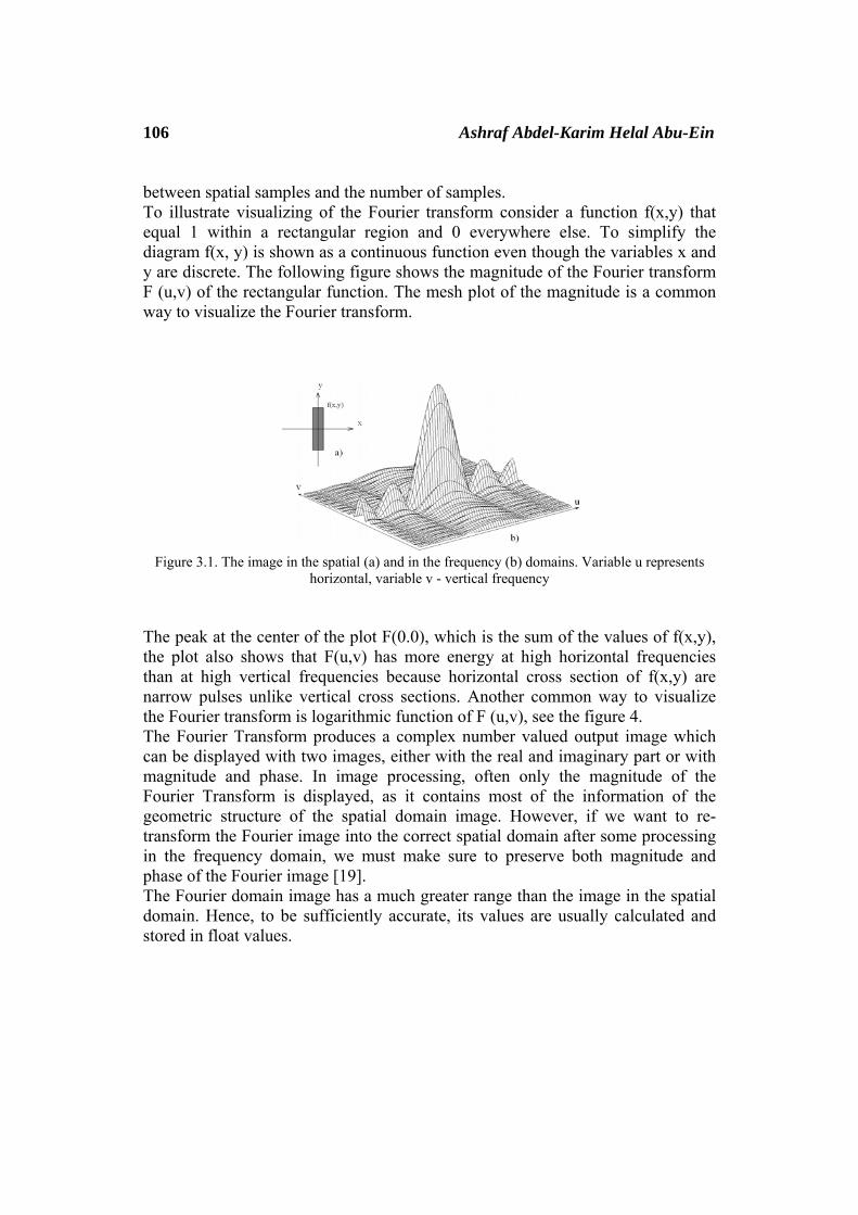
106 Ashraf Abdel-Karim Helal Abu-Ein between spatial samples and the number of samples. To illustrate visualizing of the Fourier transform consider a function f(x,y) that equal 1 within a rectangular region and 0 everywhere else. To simplify the diagram f(x, y) is shown as a continuous function even though the variables x and y are discrete. The following figure shows the magnitude of the Fourier transform F (u,v) of the rectangular function. The mesh plot of the magnitude is a common way to visualize the Fourier transform.

Figure 3.1. The image in the spatial (a) and in the frequency (b) domains. Variable u represents

horizontal, variable v - vertical frequency The peak at the center of the plot F(0.0), which is the sum of the values of f(x,y), the plot also shows that F(u,v) has more energy at high horizontal frequencies than at high vertical frequencies because horizontal cross section of f(x,y) are narrow pulses unlike vertical cross sections. Another common way to visualize the Fourier transform is logarithmic function of F (u,v), see the figure 4. The Fourier Transform produces a complex number valued output image which can be displayed with two images, either with the real and imaginary part or with magnitude and phase. In image processing, often only the magnitude of the Fourier Transform is displayed, as it contains most of the information of the geometric structure of the spatial domain image. However, if we want to re-transform the Fourier image into the correct spatial domain after some processing in the frequency domain, we must make sure to preserve both magnitude and phase of the Fourier image [19]. The Fourier domain image has a much greater range than the image in the spatial domain. Hence, to be sufficiently accurate, its values are usually calculated and stored in float values.

Novel methodology for digital removal of periodic noise 107

Figure 4 :The input image (a) in spatial domain; (b) - same image after 2D Fourier transform, spectrum of magnitude, (c) - logarithmic spectrum of the image, (d) - spectrum of phases, (e)

image in spatial domain after inverse Fourier transform, phases assigned to be equal zero, (f)- 2D Fourier transform of the image (e).

The figure 4 illustrates some examples of the Fourier transform. We start off by applying the Fourier Transform of input image 4.a, the magnitude calculated from the complex result is shown in the figure 4. b. We can see that the DC-value is by far the largest component of the image. However, the dynamic range of the Fourier coefficients (i.e. the intensity values in the Fourier image) is too large to be displayed on the screen directly. The figure b. illustrates equalized representation of magnitude spectrum of the image, low values of spectral coefficients refer to black color, high value - to white. If we apply a logarithmic transformation to the image we obtain the image c. The result shows that the image contains components of all frequencies, but that their magnitude gets smaller for higher frequencies. Hence, low frequencies contain more image information than the higher ones [6]. The transform image also tells us that there are two dominating directions in the Fourier image, one passing vertically and one horizontally through the center. These originate from the regular patterns in the background of the original image. The phase of the Fourier transform of the same image is shown in the figure d. The value of each point determines the phase of the corresponding frequency. As in the magnitude image, we can identify the vertical and horizontal lines corresponding to the patterns in the original image. The phase image does not yield much new information about the structure of the spatial domain image; therefore, in the following examples, we will restrict ourselves to displaying only the magnitude of the Fourier Transform. Before we leave the phase image entirely, however, note that if we apply the inverse Fourier Transform to the above magnitude image while ignoring the phase (assign it to be equal zero) we obtain the image e. Although this image contains the same frequencies (and amount of frequencies) as the original input image, it is corrupted beyond recognition. This shows that the phase information is crucial to reconstruct the correct image in the spatial domain. The figure f illustrates result of 2D Fourier transform of the image 4..e. As we can see, the spectrum of image 4.a. equal to the spectrum of the image 4.e.

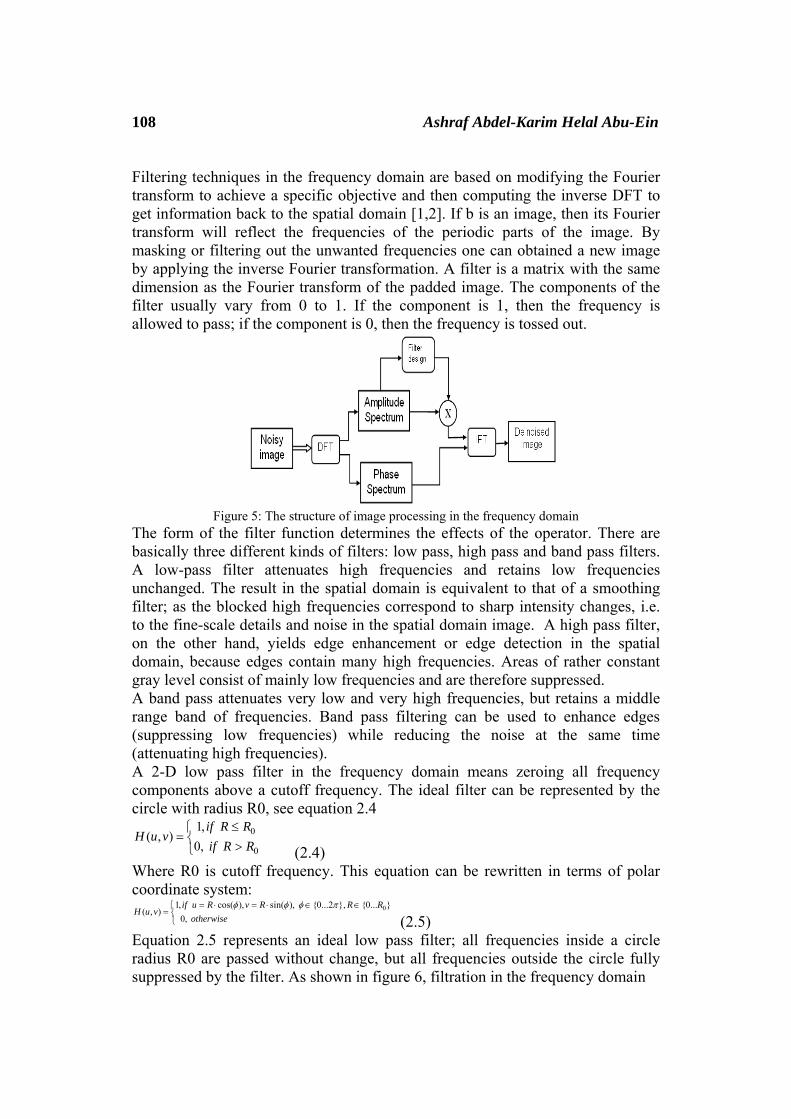
108 Ashraf Abdel-Karim Helal Abu-Ein Filtering techniques in the frequency domain are based on modifying the Fourier transform to achieve a specific objective and then computing the inverse DFT to get information back to the spatial domain [1,2]. If b is an image, then its Fourier transform will reflect the frequencies of the periodic parts of the image. By masking or filtering out the unwanted frequencies one can obtained a new image by applying the inverse Fourier transformation. A filter is a matrix with the same dimension as the Fourier transform of the padded image. The components of the filter usually vary from 0 to 1. If the component is 1, then the frequency is allowed to pass; if the component is 0, then the frequency is tossed out.

Figure 5: The structure of image processing in the frequency domain

The form of the filter function determines the effects of the operator. There are basically three different kinds of filters: low pass, high pass and band pass filters. A low-pass filter attenuates high frequencies and retains low frequencies unchanged. The result in the spatial domain is equivalent to that of a smoothing filter; as the blocked high frequencies correspond to sharp intensity changes, i.e. to the fine-scale details and noise in the spatial domain image. A high pass filter, on the other hand, yields edge enhancement or edge detection in the spatial domain, because edges contain many high frequencies. Areas of rather constant gray level consist of mainly low frequencies and are therefore suppressed. A band pass attenuates very low and very high frequencies, but retains a middle range band of frequencies. Band pass filtering can be used to enhance edges (suppressing low frequencies) while reducing the noise at the same time (attenuating high frequencies). A 2-D low pass filter in the frequency domain means zeroing all frequency components above a cutoff frequency. The ideal filter can be represented by the circle with radius R0, see equation 2.4

0

0

1, ( , )

0, if R R

H u vif R R

≤⎧= ⎨ >⎩ (2.4)

Where R0 is cutoff frequency. This equation can be rewritten in terms of polar coordinate system:

01, cos( ), sin( ), {0...2 }, {0... }( , )

0, if u R v R R R

H u votherwise

φ φ φ π= ⋅ = ⋅ ∈ ∈⎧= ⎨⎩ (2.5)

Equation 2.5 represents an ideal low pass filter; all frequencies inside a circle radius R0 are passed without change, but all frequencies outside the circle fully suppressed by the filter. As shown in figure 6, filtration in the frequency domain

Novel methodology for digital removal of periodic noise 109 using ideal low pass filter. The visual effect of low pass filtration is blurring, also it is possible to see that result has effect of "ringing", it is behavior of ideal filters. It is clear from example that ideal low pass filtering is not very practical. The following uses a smooth version of the same low pass filter (figure 6.e). Smoothed filter created by 2D filtration of ideal filter by spatial averaging filter using 23X23 masks. The ringing is greatly reduced, as possible to see in the large regions of constant (low frequency) content such as flat region of image, see figure 6.f. Some other example of non-ideal low pass filter is Butterworth filter.

A. B.

C. D.

110 Ashraf Abdel-Karim Helal Abu-Ein

E. F.

Figure 6: a) Input image, b) the spectrum of input image, c) the ideal low pass filter, d) result of filtration in spatial domain, e) smoothed low pass filter, f) result of filtration

The Butterworth filter is one type of signal processing filter design. It is designed to have a frequency response which is as flat as mathematically possible in the pass band. Another name for it is maximally flat magnitude filter. The transfer function of a Butterworth low pass filter represented below:

20

1( , )1 [ ( , ) / ] nH u v

R u v R=

+ (2.6) Where n is order of the filter, R0 is cutoff frequency. The frequency response of the Butterworth filter is maximally flat (has no ripples) in the pass band, and rolls off towards zero in the stop band. For a first-order filter, the response rolls off at −6 dB per octave (−20 dB per decade) (all first-order low pass filters have the same normalized frequency response). For a second-order low pass filter, the response ultimately decreases at −12 dB per octave, a third-order at −18 dB, and so on. Butterworth filters have a monotonically changing magnitude function with ω, unlike other filter types that have non-monotonic ripple in the pass band and/or the stop band. It is possible to see that transition band of the filter become narrow during raising the filter order. For order more than ten result of filtration contains "ringing" like for ideal low pass filter. A 2-D ideal high pass filter is defined as:

0

0

0, ( , )

1, if R R

H u vif R R

≤⎧= ⎨ >⎩ (2.7)

Novel methodology for digital removal of periodic noise 111 Definition of high pass filter can be expressed in terms of polar coordinate system:

00, cos( ), sin( ), {0...2 }, {0... }( , )

1, if u R v R R R

H u votherwise

φ φ φ π= ⋅ = ⋅ ∈ ∈⎧= ⎨⎩ (2.8)

A 2-D Butterworth high pass filter of order n defined according to the equation (2.9)

20

1( , )1 [ / ( , ) ] nH u v

R R u v=

+ (2.9) Where n is filter order, R0 - cutoff frequency. As with low pass filter, Butterworth filter smoother than the ideal. Band pass filter has two cut off frequencies R1 and R2 and allow passing a frequencies within a band from R1 to R2. Equation 2.10 represents the ideal band pass filter

1 21, cos( ), sin( ), {0...2 }, { ... }( , )

0, if u R v R R R R

H u votherwise

φ φ φ π= ⋅ = ⋅ ∈ ∈⎧= ⎨⎩ (2.10)

Unlike ban pass, band stop (band reject) filter allow to pass a frequencies within a band from zero to R1 and from R2 to infinite, the band R1...R2 in this case suppressed by a filter function. Equation 2.10 represents the ideal band stop filter

1 21, cos( ), sin( ), {0...2 }, { ... }( , )

0, if u R v R R R R

H u votherwise

φ φ φ π= ⋅ = ⋅ ∈ ∉⎧= ⎨⎩ (2.11)

Notch filter are the most useful of the selective filters. A notch filter rejects or passes frequencies in predefined regions. The notch reject filters are constructed as products of high pass filters. III. Methodology for periodic noise removal The proposed methodology consists of the following sequence of steps: Step1:Acquire the color image, apply direct conversion to convert color image to gray image and save the red and green components to be used later on in indirect conversion. Step2:Transfer the gray image representation from time domain to frequency domain by applying 2D FFT which gives us the magnitude and angle matrix of the image, save the angle matrix to be used later on. Step3:Analyze the magnitude matrix spectrum and prepare the filter mask. Step 4:Correlate the magnitude matrix with filter mask. Step 5:Use the correlated matrix and angle matrix and apply inverse FFT to get the new gray image. Step 6:Apply inverse conversion to get the cleared color image.

IV. Methodology implementation The methodology in 2 was coded using mat lab and the program was tested using various color images with periodic noises of different levels:


Step1:The following matlab code was implemented to process step1:

Figure (7) shows the results of implementing step 1

Figure (7): Results of step 1

To implement step 2, a noise was added to the gray image and 2D FFT was applied in order to get the spectrum of the image. Figure (8) shows the magnitude matrix of the image after executing the following mat lab code:

Source color image Source gray image


Figure (8): Results of step 2

Step 3 was implemented by the following matlab code by which the filter mask is calculated and prepared to be used later on in the next step, figure(9) shows the results of implementing this step:

Figure (9): results of step 3 A step 4 and 5 was implemented by the following matlab code:

FFT,magnitude of source image


The magnitude matrix was correlated fist with the filter mask, and then the result of correlation was used with the inverse FFT to obtain the denoised gray image.

V. Experimental results The above mentioned methodology was tested using various color images with different levels of low and high frequency levels of periodic noise.The same images were treated using average, median and morphological mask filters. Different parameters are used to estimate the noise level; from the obtained experimental results we can conclude that only one parameter affects the estimated mean value of the noise.Increasing No of orientations to use leads to decreasing the mean value of the noise, thus decreasing the low and high levels of the noise, at the same time increasing the number of orientation leads to increasing the image brightness.From the obtained results we can conclude that using big enough number of orientation to process a power of 2 image size leads to processing time and noise minimization.

VI. Conclusion The 2-D FFT removal algorithm for reducing the periodic noise in natural and strain images is proposed in this paper. For the periodic pattern of the artifacts, we apply the 2-D FFT on the strain and natural images to extract and remove the peaks which are corresponding to periodic noise in the frequency domain. Further the mean filter applied to get more effective results. The performance of each filter is compared using parameter PSNR (Peak Signal to Noise Ratio). The performance ofthe proposed method is tested on both natural and strain images. The results of proposed method is compared with the mean filter based periodic noise removal and found that the proposed method significantly improved for the noise removal.


REFERENCES

[1] C. Ris and S. Dupont, “Assessing local noise level estimation methods: application to noise robust ASR,” Speech Communication, vol. 34, no. 2, pp. 141–158, 2001.

[2] V. Stahl, A. Fischer, and R. Bippus, “Quantile based noise estimation for spectral subtraction and wiener filtering,” in Proc. IEEE Int. Conf. Acoust., Speech, and Sig. Proc. (ICASSP’00), Istanbul, Turkey, 2000, pp. 1875–1978.

[3] M. Alonso, R. adeau, B. David, and G. Richard, “Musical tempo estimation using noise subspace projection,” in Proc. IEEE Workshop Appl. of Dig. Sig. Proc. to Audio and Acoust., New Palz, NY, 2003, pp. 95–98.

[4] A. Röbel, M. Zivanovic, and X. Rodet, “Signal decomposition by means of classification of spectral peaks,” in Proc.Int. Comp. Music Conf. (ICMC’04), Miami, USA, 2004, pp.446–449. Barcelona, Spain, 1998.

[5] John Daugman: "Complete Discrete 2-D Gabor Transforms by Neural Networks for Image Analysis and Compression", IEEE Trans on Acoustics, Speech, and Signal Processing. Vol. 36. No. 7. July 1988, pp. 1169–1179

[6] Snakes and ladders: The role of temporal modulation in visual contour integration. Vision Research, 2001,41,3775–3782.

[7] Mood, A.; Graybill, F.; Boes, D. (1974). Introduction to the Theory of Statistics (3rd ed.). McGraw-Hill. p. 229.

[8] Relationships between orientation-preference pinwheels, cytochrome oxidase blobs, and ocular-dominance columns in primate striate cortex. Proceedings of the National Academy of Sciences of the United States of America,1998, 89, 11905–11909

[9] How long range is contour integration in human color vision? Visual Neuroscience, 2003,20, 51–64.

[10] Dynamics of collinear contrast facilitation are consistent with long-range horizontal striate transmission. Vision Research,2005, 45,2728–2739.

[11] From filters to features: Scale-space analysis of edge and blur coding in human vision. Journal of Vision,2007, 7, (13):7, 1–21, http://journalofvision.org/7/13/7/, doi:10.1167/7.13.7.

[12] Alam SK, Ophir J. Reduction of signal decorrelation from mechanical compression of tissues by temporal stretching; Applications to electrograph. Ultrasound Med Biol 1997; 23:95-105.

[13] Alam SK, Ophir J. Konofagou EE. An adaptive strain estimator forelastography. IEEE Trans UltrasonFerroelecFreq Control 1998.

[14] Varghese T and Ophir J. Cespedes I. Noise reduction in elastogram using temporal streching with muti compression averaging.Ultrasound Med Biol 1996.

[15] TechavipooU.Varghese T. Wavelet de-nosing of displacement estimates in elastography. Ultrasound Med Biol 2004a.

[16] Techavipoo U, Chen Q, Varghese T, Zagzebski JA, Madsen EL. Noise reduction using spatial-angular compounding for elastography. IEEE Trans UltrasonFerroelecFreq Control 2004b


[17] R. Gonzalez, R. Woods. Digital image processing, third edition. 2008,

Pearson Prentice Hall, ISBN 0-13-505267-X [18] Robert A. Schowengerdt Remote sensing, models, and methods for image

processing // Academic Press; 2 edition, 2007, ISBN-10: 0126289816 [19] Ballard, D.H., Brown C.M, [1990] Computer vision, Prentice Hall,

Englewood Cliffs, N.J.B, [20] Bracewell, R.N. Two Dimensional Imaging, Prentice Hall, Upper Saddle

River, N.J. [1995]. [21] Bracewell, R.N. The Fourier Transform and its Applications, 3rd ed.

Mc.Graw-Hill, New Yourk., Prentice Hall, Upper Saddle River, N.J. [2000]. [22] Pyatykh S, Hesser J, Zheng L, Image noise level estimation by principal

component analysis, IEEE transactions on image processing, vol.22, no. 2, pp.678-699, 2013.

[23] Liu X, Tanaka M, Okutomi M., Single-image Noise Level Estimation for Blind Denoising. IEEE transactions on image processing, vol.22, Issue 12, pp.5226 – 5237, 2013.

[24] Yuan,W., Lin, J., An, W., Wang, Y., Chen, N., Noise estimation based on time–frequency correlation for speech enhancement, Applied Acoustics, vol.74, Issue 5, pp.770-781, 2013. Received: October, 2013

a novel methodology for digital removal of periodic noise ... · pdf fileusing the following...

Documents