A Parallel Algorithm for Simulation of Unsteady Flows

in Multistage Turbomachinery

Paul G. A. Cizmas

Department of Aerospace Engineering

Texas A&M University

College Station, Texas 77843-3141

Ravishankar Subramanya

Pittsburgh Supercomputing Center

Pittsburgh, Pennsylvania 15213-2683

Abstract

The numerical simulation of unsteady flow in multi-stage turbomachinery is computationally

expensive. A parallel code using message-passing interface libraries, which was developed to

reduce the turnaround time and the cost of computation, is presented in this paper. The

paper describes the details of the parallel algorithm, including the parallelization rationale,

domain decomposition and processor allocation, and communication patterns. The numeri-

cal algorithm was used to simulate the unsteady flow in a six-row test turbine. The numerical

results present the salient features of the turbine flow, such as the temporal and spatial vari-

1

2

ation of velocity, pressure, temperature and blade force. To illustrate the advantages of

parallel processing, the turnaround time of the turbine flow simulation was compared on

several computers where the code was run in parallel and sequential mode.

Nomenclature

Cp - Pressure coefficient

F - Force

f - Frequency

p - Pressure

r - Radius

T - Temperature

γ - Ratio of specific heats of a gas

µ - Viscosity

ρ - Density

τ - Skin friction

ω - Angular velocity

Subscripts

F - Half-amplitude Fourier transform

hub - Hub location

n − d - Non-dimensional

tip - Tip location

−∞ - Upstream infinity

Superscripts

∗ - Total (or stagnation)

3

1. Introduction

Further development of turbomachinery design, including improved reliability and increased

efficiency, requires a better understanding of unsteady effects. Initially, the investigation of

unsteady flows in turbomachinery was done through experimental investigations [26, 17, 7, 8].

Currently the experimental results are efficiently complemented by the numerical simulations.

Although still there are differences between the experimental and computational results,

numerical simulation proves to be a powerful tool for turbomachinery improvement.

Computation of unsteady flows in turbomachinery was pioneered by Erdos et al. [9] who

solved the inviscid, compressible, two-dimensional, unsteady flow on a blade-to-blade stream

surface through a compressor stage. Koya and Kotake [18] solved the first three-dimensional

model of the rotor-stator interaction. Both Erdos’ and Koya’s codes used phase-lagged

periodic boundaries. The first spatially periodic boundary conditions, as well as the first

rotor-stator interaction model using Navier-Stokes equations, were introduced by Rai in 1985

[22].

Numerous computer codes for rotor-stator interaction simulation have been developed

meanwhile, especially in the last four years [6, 10, 16, 20, 21, 25]. Some of the unsteady

multi-row codes simulate the two-dimensional flow [10, 11, 15, 19, 21, 22] and some the

three-dimensional flow [6, 16, 20, 23, 25]. A common feature of these codes is that they all

use the time-marching method, which is notorious for being time consuming. This problem

becomes quite challenging for the three-dimensional flow simulation, especially when used for

clocking studies. For example, in the case of a 11

2-stage turbine, with the simplest vane/blade

count of 1:1:1 and a total grid point number of 2.7 million grid points, the computational time

reported on a Cray YMP C90 computer was about 21 days [13]. This type of computation

4

becomes prohibitive for a realistic vane/blade count.

The solution for reducing the high turnaround time and the associated cost of such a nu-

merical simulation was to develop a parallel code for the more cost effective massively parallel

processing platforms. The purpose of this paper is to present a methodology developed for

parallel computation of unsteady flow in multi-stage turbomachinery. The numerical imple-

mentation of this algorithm was then applied to simulate the flow in a six-row turbine. The

next section briefly presents the numerical method inherited by the parallel code from the

sequential code. The parallel computation strategy is discussed in section three. Section

four presents results of the numerical simulation of a test turbine. Conclusions and future

work suggestions are discussed in the last section.

2. Flow Model

The unsteady, compressible flow through multi-stage axial turbomachinery cascade was mod-

eled using the quasi-three-dimensional Navier-Stokes and Euler equations. The computa-

tional domain corresponding to each airfoil was divided into an inner region, near the airfoil,

and an outer region, away from the airfoil. The thin-layer Navier-Stokes equations modeled

the flow in the inner region where the viscous effects were strong, while the Euler equations

modeled the flow in the outer region, where viscous effects were weak. Some viscous effects

were nevertheless present in the outer region due to the wake of the airfoil and the wakes

coming from the upstream airfoils. However, even if the Euler equations were replaced by

the Navier-Stokes equations, the numerical dissipation in the outer region was much larger

than the viscous effects [12]. Consequently, using the Euler equations to model the region

away from the airfoil was a reasonable choice, which reduced the computational time. The

flow was assumed to be fully turbulent and the turbulent viscosity was modeled using the

5

Baldwin-Lomax algebraic model.

The Euler and Navier-Stokes equations written in strong conservative form were inte-

grated using a third-order-accurate, iterative, implicit, upwind scheme. The integration

scheme was inherited from the sequential code developed by Rai [22] and details can be

found in the paper by Rai and Chakravarthy [24]. The nonlinear finite-difference approxi-

mation was solved iteratively at each time level using an approximate factorization method.

Between two and four Newton iterations were used at each time step to reduce the associated

linearization and factorization error.

Grid Generation

The computational domain around the airfoil, where the effects of viscosity were important,

was discretized by an O-grid. This O-grid, generated using an elliptical method, was used

to resolve the flow modeled by the Navier-Stokes equations. The O-grid was overlaid on top

of an H-grid. The H-grid was used to discretize the computational domain away from the

airfoil, where viscous effects were less important. In this region the flow was modeled by the

Euler equations. The H-grid was algebraically generated.

The flow variables were communicated between the O- and the H-grids through bilinear

interpolation. The O-grid must overlay for more than two grid cells on top of the H-grid

to provide good communication of the flow variables between the two grids. An excessive

overlay of the O- and the H-grids causes an useless increase of the grid points of the O-

grids and consequently a longer computational time. The flow variables were communicated

between two adjacent rows through the H-grids. The patched H-grids corresponding to the

rotating and stationary grids slipped past each other to model the relative motion. The

H-grids could be either overlaid or abut. The results presented in this paper were obtained

6

using only abut grids.

Boundary Conditions

Two classes of boundary conditions were enforced on the grid boundaries: natural boundary

conditions and zonal boundary conditions. The natural boundaries included inlet, outlet,

periodic and the airfoil surfaces. The zonal boundaries, required by the use of multiple grids,

included patched and overlaid boundaries.

At the airfoil surface, no-slip, adiabatic wall and zero pressure gradient conditions were

enforced. The adiabatic wall condition and the pressure gradient condition were implemented

in an implicit manner. For the blade, the no-slip boundary condition enforced that the fluid

velocity at the blade surface was equal to the rotor speed [22].

The inlet boundary conditions specified flow angle, average total pressure and down-

stream propagating Riemann invariant. The upstream propagating Riemann invariant was

extrapolated from the interior of the domain. At the outlet, the average static pressure was

specified, while the downstream propagating Riemann invariant, circumferential velocity,

and entropy were extrapolated from the interior of the domain. Periodicity was enforced by

matching flow conditions between the lower surface of the lowest H-grid of a row and the

upper surface of the top most H-grid of the same row.

For the zonal boundary conditions of the overlaid boundaries, data were transferred from

the H-grid to the O-grid along the O-grid’s outermost grid line. Data were then transferred

back to the H-grid along its inner boundary. At the end of each iteration an explicit,

corrective, interpolation procedure was performed. The outer boundaries of the O-grids

were interpolated from the interior grid points of the H-grids. The inner boundaries of the

H-grids were interpolated from the interior grid points of the O-grids. Stability improved by

7

increasing the overlap area of the O- and H-grids [14]. The patch boundaries were treated

similarly, using linear interpolation to update data between adjoint grids [22].

3. Parallel Computation

The high turnaround time and the associated cost of running a sequential code to simulate

the rotor-stator interaction is unacceptable for the turbomachinery design process. To reduce

the turnaround time and cost per mega floating point operations per second (MFLOP), the

Parallel Rotor-Stator Interaction quasi-three-dimensional (PaRSI) code was developed based

on the sequential code STAGE-2 [14]. The parallel code uses message-passing interface (MPI)

libraries and runs on symmetric multi-processors (Silicon Graphics Challenge) and massively

parallel processors (Cray T3E). The parallel code should run with minor modifications on

all platforms that support MPI.

The computational grid was divided into blocks. Here a block was defined as a collection

of grid points. One processor was allocated for each block. One block was associated to each

airfoil. Each airfoil block included the O- and H-grid associated to that airfoil. Each inlet

and outlet blocks included only an H-grid.

The Navier-Stokes/Euler equations were solved within each block. At every time-step,

the solver swept all the airfoil rows from left to right, visiting each block of the row from

bottom to top. Boundary conditions between grids were enforced by storing and retrieving

neighboring boundary values in/from a global shared vector. This code structure greatly

facilitated the development of a multiple instruction multiple data (MIMD) version of the

code.

8

Design Rationale

The main idea behind the effort was to reuse as much as possible the data structures and

solution procedures from the original code without sacrificing parallel efficiency. Coarse

grained parallelism consistent with a message passing paradigm appeared to be the intuitive

approach to maximize the computation to communication ratio. Extendibility of the code to

three dimensions was accounted for in designing the communication patterns. A side-effect

of the concurrency introduced by parallelizing the code was the ability to step all the grids in

time at the same instant. This qualitatively improved the original algorithm which updated

the solution at each time step using a sweep pattern.

Domain Decomposition

The multiple-grid domain was decomposed by allocating one block to each processor, as

shown in Figure 1. One processor was allocated for each inlet and outlet H-grid. One

processor was allocated for each pair of O- and H-grids corresponding to each airfoil. The

overlay of the O- and H-grids is necessary to exchange information between the viscous

computation in the O-grid and the inviscid computation in the H-grid. This overlay would

have greatly complicated communication patterns if the O- and H-grids were located on

different processors. Since the code was not memory bound, we bypassed the problem by

allocating both H- and O-grids of a given airfoil to the same processor.

This processor allocation introduced problems of load balancing the inlet and outlet grids

that had fewer grid points than the airfoil grids. Load balancing was done by extending the

inlet and outlet grids and increasing the extent of the computational domain. This has the

added benefit of moving the inlet and outlet boundaries away from the airfoils. Consequently,

the harmful influence of the outgoing-wave reflections on the solution was reduced and the

9

convergence speed and the accuracy of results improved.

Figure 2 illustrates the processor element (PE) numbering adopted to decompose the

domains and the topology created as a consequence. Each PE was uniquely identified by

a global PE number (G PE). Within each subdomain, PEs were uniquely identified by a

subdomain PE number (X PE and Y PE) based on the subdomain’s major axis. Global PE

numbering was bottom to top, left to right. PE numbering along x-axis was left to right.

PE numbering along y-axis was left to right. PE values of -1 means that the variable was

undefined.

I/O Parallelization

Sequential input grid and flow data files were split using a preprocessor which generated grid

and flow data files corresponding to each processor. Each processor then read in the grid and

flow data conditions in parallel and wrote out checkpoint data and results to multiple files in

parallel. The improved parallel I/O performance of the Cray T3E computers ensured that

this step was not a performance bottleneck for the code. A postprocessor then aggregated the

result data sets into a single file suitable for further processing in a visualization application.

Communication Patterns

The communication patterns between the processors were driven by the need to enforce

boundary conditions between grids and the need to perform global reduction operations once

every time step. Global reduction operations were performed by using MPI ALL REDUCE.

Communication groups were created to take care of communication along different axes. Fig-

ure 3 illustrates the communication patterns implemented for enforcing boundary conditions

between grids.

10

Periodic boundary conditions were enforced along the x−axis and were imposed by cyclic

communication patterns within rows. Processors along the x−axis were associated with a

unique communicator ICOMM and use MPI SENDRECEIVE to exchange boundary values.

The communication patterns were general and extend to arbitrary number of PEs on the

same stage.

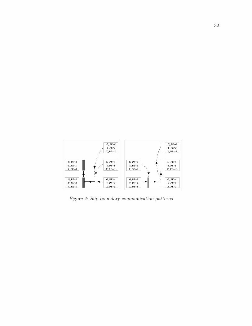
Slip conditions between columns of processors posed a more difficult problem. The dy-

namic nature of the slip boundary implied changing message sizes between senders and

receivers. We simplified the problem by performing a gather of all the slip boundary values

along the y−axis, exchanging the vector with the neighboring column and then broadcasting

it along the y−axis. The left side of Fig. 4 illustrates the communication pattern from the

right row of blades to the left row of blades. The right side of Fig. 4 illustrates the com-

munication from the left row of blades to the right row of blades. The two communications

from right to left and from left to right took place simultaneously.

4. Numerical Results

The parallel computation algorithm presented in the previous section was implemented in

the PaRSI code. This code was successfully used to predict the rotor-stator interaction in

a combustion turbine [5], and to analyze rotor and stator multi-stage clocking in a steam

turbine [2]. In this paper, the parallel code was used to simulate the unsteady flow in a six-

row turbine. This section presents the validation of the accuracy of the numerical results, a

comparison of computational time on different computers, and a set of results that illustrate

some salient features of the unsteady turbine flow.

11

Turbine Description

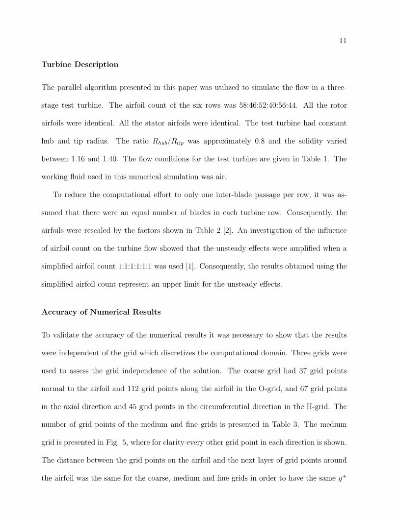
The parallel algorithm presented in this paper was utilized to simulate the flow in a three-

stage test turbine. The airfoil count of the six rows was 58:46:52:40:56:44. All the rotor

airfoils were identical. All the stator airfoils were identical. The test turbine had constant

hub and tip radius. The ratio Rhub/Rtip was approximately 0.8 and the solidity varied

between 1.16 and 1.40. The flow conditions for the test turbine are given in Table 1. The

working fluid used in this numerical simulation was air.

To reduce the computational effort to only one inter-blade passage per row, it was as-

sumed that there were an equal number of blades in each turbine row. Consequently, the

airfoils were rescaled by the factors shown in Table 2 [2]. An investigation of the influence

of airfoil count on the turbine flow showed that the unsteady effects were amplified when a

simplified airfoil count 1:1:1:1:1:1 was used [1]. Consequently, the results obtained using the

simplified airfoil count represent an upper limit for the unsteady effects.

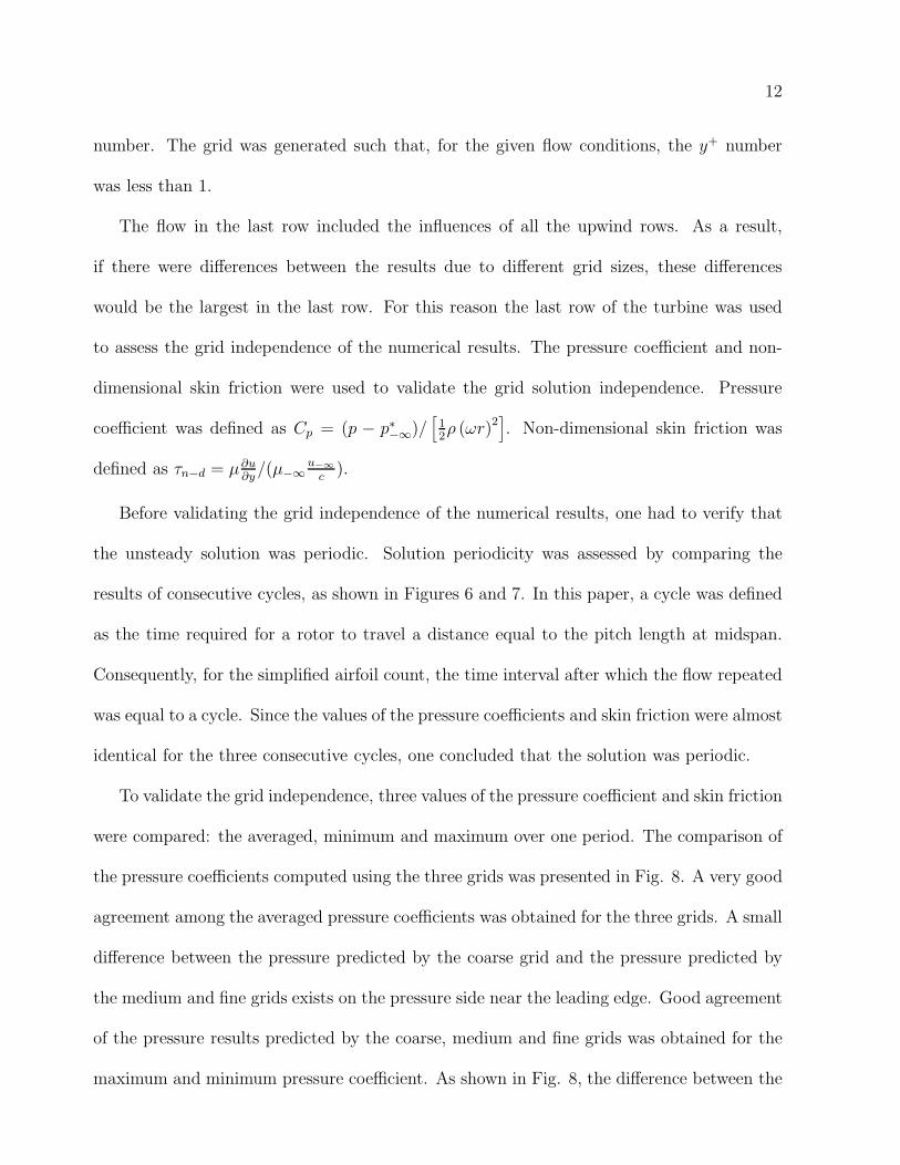
Accuracy of Numerical Results

To validate the accuracy of the numerical results it was necessary to show that the results

were independent of the grid which discretizes the computational domain. Three grids were

used to assess the grid independence of the solution. The coarse grid had 37 grid points

normal to the airfoil and 112 grid points along the airfoil in the O-grid, and 67 grid points

in the axial direction and 45 grid points in the circumferential direction in the H-grid. The

number of grid points of the medium and fine grids is presented in Table 3. The medium

grid is presented in Fig. 5, where for clarity every other grid point in each direction is shown.

The distance between the grid points on the airfoil and the next layer of grid points around

the airfoil was the same for the coarse, medium and fine grids in order to have the same y+

12

number. The grid was generated such that, for the given flow conditions, the y+ number

was less than 1.

The flow in the last row included the influences of all the upwind rows. As a result,

if there were differences between the results due to different grid sizes, these differences

would be the largest in the last row. For this reason the last row of the turbine was used

to assess the grid independence of the numerical results. The pressure coefficient and non-

dimensional skin friction were used to validate the grid solution independence. Pressure

coefficient was defined as Cp = (p − p∗−∞

)/[

1

2ρ (ωr)2

]

. Non-dimensional skin friction was

defined as τn−d = µ∂u∂y

/(µ−∞

u−∞

c).

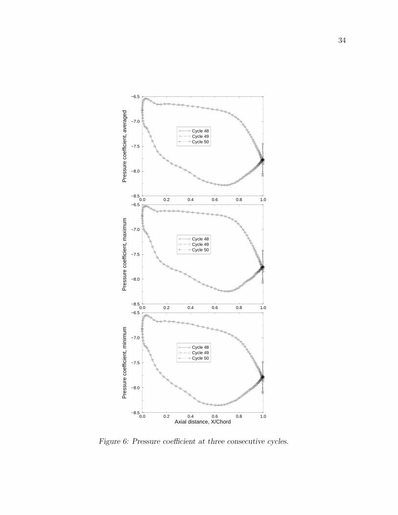
Before validating the grid independence of the numerical results, one had to verify that

the unsteady solution was periodic. Solution periodicity was assessed by comparing the

results of consecutive cycles, as shown in Figures 6 and 7. In this paper, a cycle was defined

as the time required for a rotor to travel a distance equal to the pitch length at midspan.

Consequently, for the simplified airfoil count, the time interval after which the flow repeated

was equal to a cycle. Since the values of the pressure coefficients and skin friction were almost

identical for the three consecutive cycles, one concluded that the solution was periodic.

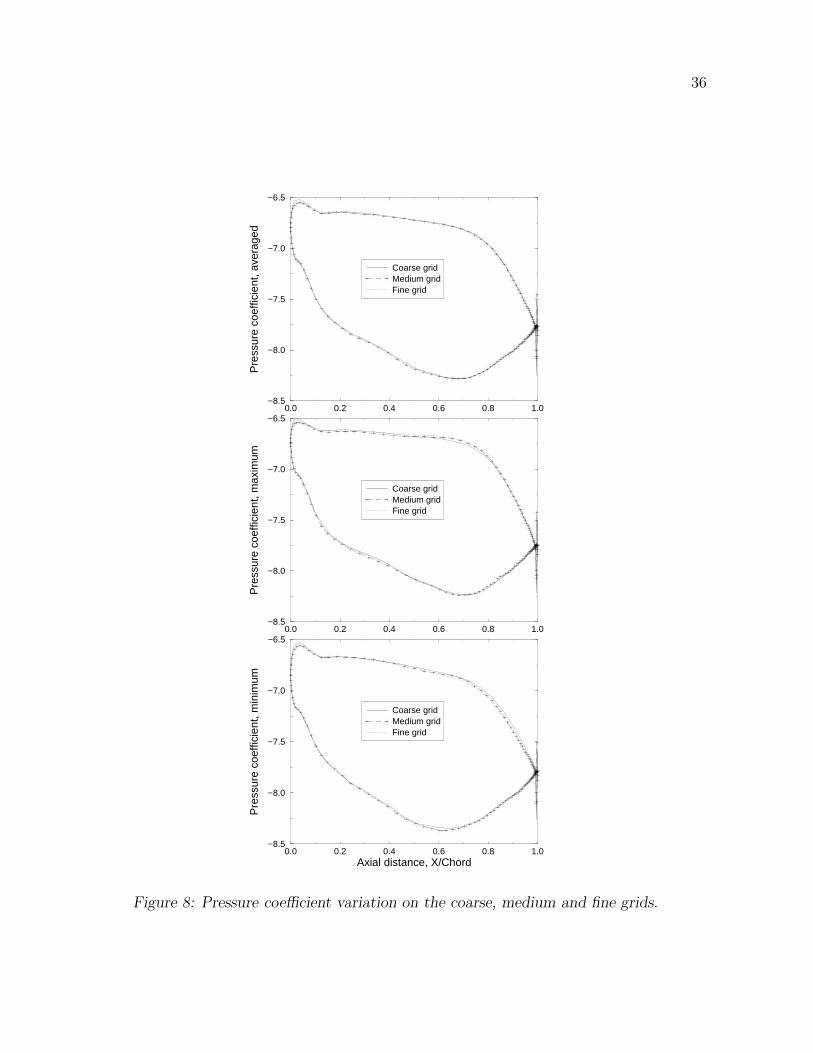
To validate the grid independence, three values of the pressure coefficient and skin friction

were compared: the averaged, minimum and maximum over one period. The comparison of

the pressure coefficients computed using the three grids was presented in Fig. 8. A very good

agreement among the averaged pressure coefficients was obtained for the three grids. A small

difference between the pressure predicted by the coarse grid and the pressure predicted by

the medium and fine grids exists on the pressure side near the leading edge. Good agreement

of the pressure results predicted by the coarse, medium and fine grids was obtained for the

maximum and minimum pressure coefficient. As shown in Fig. 8, the difference between the

13

pressure coefficient corresponding to the three grids was less than 0.6%.

The comparison of the skin friction coefficients computed using the three grids is shown

in Fig.9. Good agreement was obtained between the results corresponding to the medium

and fine grid, the difference being less than 2%. The difference between the coarse grid

skin friction and the medium or fine grid skin friction was significantly larger. The largest

difference was approximately 7.7%, shown on the pressure side of the maximum skin friction.

As a result, one concluded that the numerical results were grid independent only for the

medium and fine grids. The medium grid was used for the computation of all subsequent

results throughout the paper.

The grid convergence analysis showed that pressure coefficient was not a reliable indicator

for viscous flows. As shown above, pressure coefficient did not detect that the coarse grid

was producing results that were significantly affected by the mesh size. Pressure coefficient

did not capture viscous effects and, as a result, should not be used as the only indicator for

the grid convergence analysis of viscous flows. Consequently, to validate that the results of

viscous flow simulation are independent of the grid size, it is necessary to use skin friction

or other indicator that is strongly dependent of viscosity.

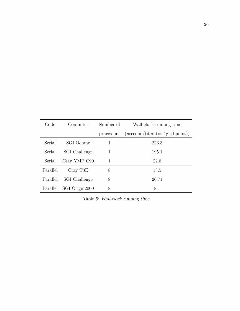
Computational Time Comparison

The parallel code was implemented on Cray T3E, SGI Challenge, and SGI Origin 2000

computers. Eight processors were used for the parallel computation, as shown in Fig. 5. The

sequential code was benchmarked on a SGI Octane, a SGI Challenge and a Cray YMP C90

computer. The specifications of the target platforms is presented in Table 4. The comparison

of the turnaround time is presented in Table 5.

The following observations resulted from the timings shown in Table 5.

14

• The differences in the single processor times of the SGI Challenge and the Octane arose

from the differences in memory availability on the two platforms. The larger memory

available on the Challenge reduced wall-time by eliminating process-swapping to disk.

• Vectorization on the Cray C90 considerable reduced the elapsed time for the code. The

code was characterized by strided sequential memory access that took advantage of the

vector pipeline on the C90.

• The efficiency of the MPI implementation was demonstrated by the close to linear

speedup observed between the single processor run on the SGI Challenge and the 8

processor run.

• The code scaled equally well on a distributed memory machine (MPP) such as the

T3E, a symmetric multi-processing machine (SMP) such as the SGI Challenge and a

ccNUMA (Cache Coherent Non-Uniform Memory Access) platform such as the Origin

2000. This was due to the efficient structuring of the communication patterns and

predominance of nearest neighbor communications. The high bandwidth, low latency

network of the T3E also helped minimize communication overhead.

• The peak CPU performance of the EV5 processor was greater than that of the R10000

processor at 250 MHz, but the availability of larger cache on the SGI Origin 2000 gave

it a performance edge in sustained FLOPS over the T3E processors. As expected, the

SGI Challenge with slower processors (195 MHz) had compute-times slower than the

T3E.

15

Test Turbine Results

The parallel algorithm presented in the previous sections was used to simulate the unsteady

flow in a three-stage test turbine. This turbine was previously used to investigate rotor and

stator clocking [2]. Same turbine was used to investigate the influence of the gap on the

efficiency and turbine losses [4]. This section focuses on the analysis of unsteady pressure,

temperature and airfoil forces in the turbine.

Figure 10 shows the locations where the static pressures and static temperatures were

evaluated. For each airfoil, pressure and temperature values were presented for the suction

and pressure side. The variation of non-dimensional temperature on the turbine blades and

vanes is shown in Fig. 11.

The non-dimensional temperature was defined in this analysis as Tn−d = γT/T ∗

−∞. As

expected, the temperature decreased from the first vane to the last blade. For each vane

or blade, the temperature was larger on the pressure side than on the suction side. The

amplitude of temperature variation was larger on the suction side than on the pressure side,

as summarized in Table 6. The temperature amplitudes increase in the downstream direction,

except for the pressure side of the blades, where the amplitude was almost constant.

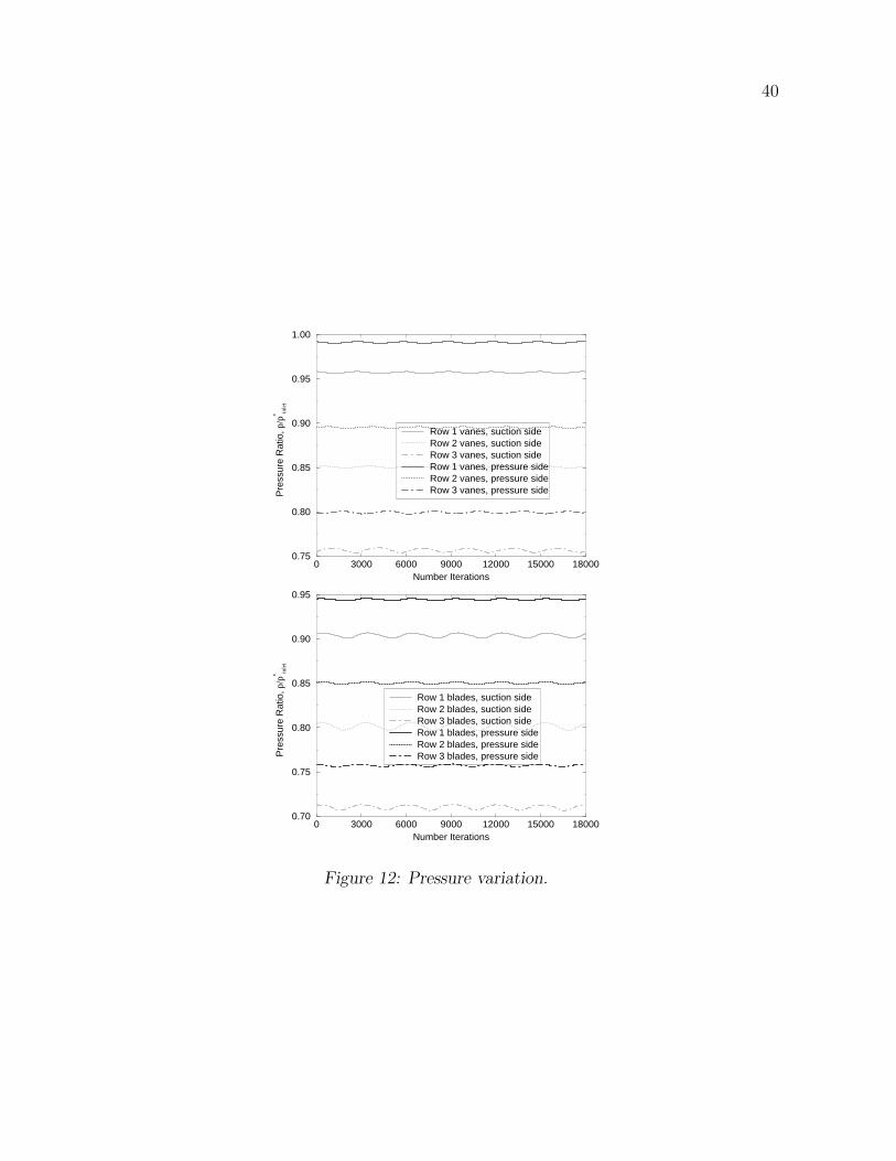
Figure 12 displays the non-dimensional pressure variation on blades and vanes. The

amplitudes of pressure variation were presented in Table 7. Especially for blades, the ampli-

tudes of pressure variation were larger on the suction side than on the pressure side. On the

vanes, the values of pressure amplitudes were approximately equal for the pressure side and

suction side. On the blades, the pressure amplitudes were at least two times larger than on

the suction side.

The time variation of vane and blade forces is shown in Fig. 13. The non-dimensional

16

force Fn−d was defined as Fn−d =∫

C pn−dds, where C is the airfoil contour length and pn−d

is the non-dimensional pressure pn−d = p/p∗−∞

. The length s was non-dimensionalized by

the axial chord of the first vane. Figure 13 shows that vane forces were larger than blade

forces. The largest values of the unsteady forces were on the first-stage vanes, while the

lowest values were on second-stage blades.

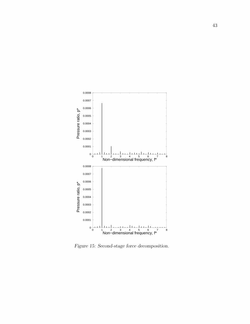
The Fourier transform of the non-dimensional forces Fn−d of the turbine airfoils is shown

in Figs. 14-16. The force FF shown in Figs. 14-16 was defined as half-amplitude Fourier

transform of the non-dimensional force Fn−d. The non-dimensional frequency fn−d was de-

fined as the ratio between the frequency and the airfoil passing frequency. For a rotational

speed of 2400 rot/min and 58 blades, the passing frequency was 2320 Hz. As expected,

Figs. 14-16 show that the largest component of the force amplitude corresponds to the air-

foil passing frequency. The largest force amplitude was located on the second-stage rotor,

while the lowest value was on the third-stage rotor. The next largest force amplitude cor-

responds to twice the airfoil passing frequency. The force amplitudes corresponding to the

other frequencies were, in general, small compared to the force amplitudes corresponding to

the airfoil passing frequency and twice the airfoil passing frequency.

5. Conclusions

The focus of this paper was to present a parallel algorithm developed for the simulation of

unsteady flow in turbomachinery cascades. The algorithm was implemented in a computer

code that was extensively tested and utilized in the last four years for numerical simulation

of flow in turbomachinery cascades [5, 2, 3, 1, 4]. The numerical scheme used Message-

Passing Interface libraries and was implemented on different parallel computers. For the

geometry presented in this analysis, where the grid was distributed over eight processors,

17

the turnaround time was reduced to approximately 20 minutes per cycle on a SGI Origin2000

computer. Since approximately 40 cycles were usually sufficient to obtain a periodic solution,

the present parallel computation showed that the wall-clock time necessary for simulation

of quasi-three-dimensional unsteady flow in turbomachinery cascades can be reduced to

approximately 13 hours. This conclusion is true for any number of rows and airfoils per row,

as long as one processor is allocated to each airfoil. A less than one day turnaround time

can also be obtained while simulating fully three-dimensional flows, if enough processors are

available to be distributed along the airfoil, in the spanwise direction.

6. Acknowledgments

The authors wish to thank the Westinghouse Electric Corporation for supporting this work.

The authors are thankful to Pittsburgh Supercomputing Center and Texas A&M Supercom-

puting Center for making the computing resources available.

References

[1] P. G. A. Cizmas. Transition and blade count influence on steam turbine clocking. Tech-

nical report, Texas Engineering Experiment Station, College Station, Texas, January

1999.

[2] P. G. A. Cizmas and D. J. Dorney. Parallel computation of turbine blade clocking.

International Journal of Turbo & Jet-Engines, 16(1):49–60, 1999.

[3] P. G. A. Cizmas and D. J. Dorney. The influence of clocking on unsteady forces of com-

pressor and turbine blades. International Journal of Turbo & Jet-Engines, 17(2):133–

142, 2000.

18

[4] P. G. A. Cizmas, C. R. Hoenninger, S. Chen, and H. F. Martin. Influence of inter-

row gap value on turbine losses. In The Eight International Symposium on Transport

Phenomena and Dynamics of Rotating Machinery (ISROMAC-8), Honolulu, Hawaii,

March 2000.

[5] P. G. A. Cizmas and R. Subramanya. Parallel computation of rotor-stator interaction.

In Torsten H. Fransson, editor, The Eight International Symposium on Unsteady Aero-

dynamics and Aeroelasticity of Turbomachines, pages 633–643, Stockholm, Sweden, Sep.

1997.

[6] R. L. Davis, T. Shang, J. Buteau, and R. H. Ni. Prediction of 3-D unsteady flow

in multi-stage turbomachinery using an implicit dual time-step approach. In 32nd

AIAA/ASME/SAE/ASEE Joint Propulsion Conference and Exhibit, AIAA Paper 96-

2565, Lake Buena Vista, FL, Jul. 1996.

[7] R. P. Dring, H. D. Joslyn, L. W. Hardin, and J. H. Wagner. Turbine rotor-stator

interaction. Transaction of the ASME: Journal of Engineering for Power, 104:729–742,

1982.

[8] M. G. Dunn, W. A. Bennett, R. A. Delaney, and K. V. Rao. Investigation of unsteady

flow through a transonic turbine stage: Data/prediction comparison for time-averaged

and phase-resolved pressure data. Transaction of the ASME: Journal of Turbomachin-

ery, 114:91–99, 1992.

[9] J. I. Erdos, E. Alzner, and W. McNally. Numerical solution of periodic transonic flow

through a fan stage. AIAA Journal, 15(11):1559–1568, Nov. 1977.

19

[10] F. Eulitz, K. Engel, and H. Gebbing. Numerical investigation of the clocking effects in

a multistage turbine. In International Gas Turbine and Aeroengine Congress, ASME

Paper 96-GT-26, Birmingham, UK, June 1996.

[11] A. Fourmaux. Unsteady flow calculation in cascades. In Proceedings of the Interna-

tional Gas Turbine Conference and Exhibit, ASME Paper 86-GT-178, Dusseldorf, West

Germany, Jun. 1986.

[12] L. W. Griffin, F. W. Huber, and O. P. Sharma. Performance improvement through

indexing of turbine airfoils: Part II - numerical simulation. Transaction of the ASME:

Journal of Turbomachinery, 118(3):636–642, October 1996.

[13] K. L. Gundy-Burlet and D. J. Dorney. Three-dimensional study of heat transfer effects

on hot streak migration. International Journal of Turbo and Jet Engines, 14(3):123–132,

1997.

[14] K. L. Gundy-Burlet, M. M. Rai, and R. P. Dring. Two-dimensional computations of

multi-stage compressor flows using a zonal approach. In 25th AIAA/ASME/SAE/ASEE

Joint Propulsion Conference, AIAA Paper 89-2452, Monterey, CA, Jul. 1989.

[15] P. C. E Jorgenson and R. V. Chima. An explicit Runge-Kutta method for unsteady

rotor/stator interaction. In 26th AIAA Aerospace Science Meeting, AIAA Paper 88-

0049, Reno, NV, Jan. 1988.

[16] A. R. Jung, J. F. Mayer, and H. Stetter. Simulation of 3D-unsteady stator/rotor in-

teraction in turbomachinery stages of arbitrary pitch ratio. In Proceedings of the 1996

International Gas Turbine and Aeroengine Congress & Exhibition, ASME Paper 96-

GT-69, Birmingham, UK, Jun. 1996.

20

[17] M. G. Kofskey and W. J. Nusbaum. Aerodynamic evaluation of two-stage axial flow

turbine designed for brayton-cycle space power system. Technical Report NASA-TN-D-

4382, National Aeronautics and Space Administration. Lewis Research Center, Cleve-

land, Ohio, February 1968.

[18] M. Koya and S. Kotake. Numerical analysis of fully three-dimensional periodic flows

through a turbine stage. In 30th International Gas Turbine Conference and Exhibit,

ASME Paper 85-GT-57, Houston, TX, 1985.

[19] J. P. Lewis, R. A. Delaney, and E. J. Hall. Numerical prediction of turbine vane-

blade aerodynamic interaction. In 23rd AIAA/SAE/ASME/ASEE Joint Propulsion

Conference, AIAA Paper 87-2149, San Diego, CA, Jun. 1987.

[20] N. Liamis, J. L. Bacha, and F. Burgaud. Numerical simulation of stator-rotor interaction

on compressor blade rows. In The 85th Propulsion and Energetics Panel Symposium on

Loss Mechanisms and Unsteady Flows in Turbomachines, Derby, UK, 1995.

[21] V. Michelassi, P. Adami, and F. Martelli. An implicit algorithm for stator-rotor inter-

action analysis. In Proceedings of the 1996 International Gas Turbine and Aeroengine

Congress & Exhibition, ASME Paper 96-GT-68, Birmingham, UK, Jun. 1996. ASME.

[22] M. M. Rai. Navier-Stokes simulation of rotor-stator interaction using patched and

overlaid grids. In AIAA 7th Computational Fluid Dynamics Conference, AIAA Paper

85-1519, Cincinnati, Ohio, 1985.

[23] M. M. Rai. Unsteady three-dimensional Navier-Stokes simulation of turbine rotor-stator

interaction. In 23rd AIAA/SAE/ASME/ASEE Joint Propulsion Conference, AIAA

Paper 87-2058, San Diego, CA, Jul. 1987.

21

[24] M. M. Rai and S. Chakravarthy. An implicit form for the Osher upwind scheme. AIAA

Journal, 24:735–743, 1986.

[25] F. L. Tsung, J. Loellbach, and C. Hah. Development of an unsteady unstructured

Navier-Stokes solver for stator-rotor interaction. In 32nd AIAA/ASME/SAE/ASEE

Joint Propulsion Conference, AIAA Paper 96-2668, Lake Buena Vista, FL, Jul. 1996.

[26] J. R. Weske. Three-dimensional flow in axial flow turbomachines. Technical Report

AFOSR211, Institute for Fluid Dynamics and Applied Mathematics, Univ of Maryland

College Park, August 1960.

22

Inlet Mach number Minlet = 0.073

Reynolds number Re = 53500

Inlet temperature Tinlet = 20 C

Pressure ratio pexit/p∗

inlet = 0.71

Rotational speed n = 2400 rot/min

Table 1: Turbine flow conditions.

23

Airfoil Rescaling factor

First-stage stator 1

First-stage rotor 46/58

Second-stage stator 52/58

Second-stage rotor 40/58

Third-stage stator 56/58

Third-stage rotor 44/58

Table 2: Airfoil rescaling factors.

24

O-grid points H-grid points

Coarse grid 112x37 67x45

Medium grid 150x50 90x60

Fine grid 180x60 108x72

Table 3: Grid points for the coarse, medium and fine grid.

25

Computer Processor type Number of Total RAM Architecture

processors

SGI Octane R10000, 195 MHz 1 384 MB Uni-processor

SGI Challenge R10000, 195 MHz 12 1024 MB SMP

SGI Origin2000 R10000, 250 MHz 32 8192 MB SMP

Cray YMP-C90 C90, 150 MHz 16 4096 MB Vector Processor

Cray T3E Alpha-EV5, 450 MHz 512 128 MB/PE MPP

Table 4: Hardware specifications of target platforms.

26

Code Computer Number of Wall-clock running time

processors (µsecond/(iteration*grid point))

Serial SGI Octane 1 223.3

Serial SGI Challenge 1 195.1

Serial Cray YMP C90 1 22.6

Parallel Cray T3E 8 13.5

Parallel SGI Challenge 8 26.71

Parallel SGI Origin2000 8 8.1

Table 5: Wall-clock running time.

27

Vane 1 Vane 2 Vane 3 Blade 1 Blade 2 Blade 3

Pressure side 0.0008 0.0012 0.0024 0.0015 0.0014 0.0013

Suction side 0.0010 0.0015 0.0042 0.0039 0.0060 0.0070

Table 6: Amplitude of non-dimensional temperature variation.

28

Vane 1 Vane 2 Vane 3 Blade 1 Blade 2 Blade 3

Pressure side 0.0019 0.0024 0.0031 0.0027 0.0028 0.0029

Suction side 0.0023 0.0022 0.0048 0.0057 0.0086 0.0062

Table 7: Amplitude of non-dimensional pressure variation.

29

Figure 1: Processors allocation for single-stage geometry.

30

G_PE=0

Y_PE=0

X_PE=0

Y_PE=0 Y_PE=0X_PE=1

Y_PE=0

G_PE=2

G_PE=3G_PE=1

Y_PE=1 Y_PE=1 Y_PE=1 Y_PE=1

Y_PE=2Y_PE=2

X_PE=2 X_PE=3

X_PE=-1 X_PE=-1 X_PE=-1 X_PE=-1

X_PE=-1 X_PE=-1

G_PE=4 G_PE=7

G_PE=5 G_PE=8

G_PE=6 G_PE=9

Y

X

Figure 2: Domain decomposition over 10 processors.

31

Y_PE=0 Y_PE=0

X_PE=1 X_PE=2

X_PE=-1 X_PE=-1

X_PE=-1

Y_PE=1

Y_PE=2

Y_PE=1

G_PE=2

G_PE=3

Y

X

G_PE=4

G_PE=5

G_PE=6

Figure 3: Periodic communications in the same row.

32

Y_PE=0Y_PE=0

X_PE=2X_PE=1

G_PE=2

G_PE=3

G_PE=4

G_PE=5

G_PE=6

Y_PE=1 Y_PE=1

Y_PE=2

X_PE=-1 X_PE=-1

X_PE=-1

Y_PE=0Y_PE=0

X_PE=2X_PE=1

G_PE=2

G_PE=3

G_PE=4

G_PE=5

G_PE=6

Y_PE=1 Y_PE=1

Y_PE=2

X_PE=-1 X_PE=-1

X_PE=-1

Figure 4: Slip boundary communication patterns.

33

Figure 5: Medium grid (every other point in each direction shown).

34

0.0 0.2 0.4 0.6 0.8 1.0−8.5

−8.0

−7.5

−7.0

−6.5

Pre

ssur

e co

effic

ient

, ave

rage

dCycle 48Cycle 49Cycle 50

0.0 0.2 0.4 0.6 0.8 1.0−8.5

−8.0

−7.5

−7.0

−6.5

Pre

ssur

e co

effic

ient

, max

imum

Cycle 48Cycle 49Cycle 50

0.0 0.2 0.4 0.6 0.8 1.0Axial distance, X/Chord

−8.5

−8.0

−7.5

−7.0

−6.5

Pre

ssur

e co

effic

ient

, min

imum

Cycle 48Cycle 49Cycle 50

Figure 6: Pressure coefficient at three consecutive cycles.

35

0 0.2 0.4 0.6 0.8 1−50

0

50

100

150

200

250

300

Ski

n fr

ictio

n, a

vera

ged

Cycle 48Cycle 49Cycle 50

0 0.2 0.4 0.6 0.8 1−50

0

50

100

150

200

250

300

Ski

n fr

ictio

n, m

axim

um

Cycle 48Cycle 49Cycle 50

0 0.2 0.4 0.6 0.8 1Axial distance, X/Chord

−50

0

50

100

150

200

250

300

Ski

n fr

ictio

n, m

inim

um

Cycle 48Cycle 49Cycle 50

Figure 7: Skin friction at three consecutive cycles.

36

0.0 0.2 0.4 0.6 0.8 1.0−8.5

−8.0

−7.5

−7.0

−6.5

Pre

ssur

e co

effic

ient

, ave

rage

dCoarse gridMedium gridFine grid

0.0 0.2 0.4 0.6 0.8 1.0−8.5

−8.0

−7.5

−7.0

−6.5

Pre

ssur

e co

effic

ient

, max

imum

Coarse gridMedium gridFine grid

0.0 0.2 0.4 0.6 0.8 1.0Axial distance, X/Chord

−8.5

−8.0

−7.5

−7.0

−6.5

Pre

ssur

e co

effic

ient

, min

imum

Coarse gridMedium gridFine grid

Figure 8: Pressure coefficient variation on the coarse, medium and fine grids.

37

0 0.2 0.4 0.6 0.8 1−100

0

100

200

300

Ski

n fr

ictio

n, a

vera

ged

Coarse gridMedium gridFine grid

0 0.2 0.4 0.6 0.8 1−100

0

100

200

300

Ski

n fr

ictio

n, m

axim

um

Coarse gridMedium gridFine grid

0 0.2 0.4 0.6 0.8 1Axial distance, X/Chord

−100

0

100

200

300

Ski

n fr

ictio

n, m

inim

um

Coarse gridMedium gridFine grid

Figure 9: Skin friction variation on the coarse, medium and fine grids.

38

Figure 10: Locations of pressure and temperature measurement.

39

0 3000 6000 9000 12000 15000 18000Number Iterations

1.31

1.33

1.35

1.37

1.39

1.41

Tem

pera

ture

Row 1 vanes, suction sideRow 2 vanes, suction sideRow 3 vanes, suction sideRow 1 vanes, pressure sideRow 2 vanes, pressure sideRow 3 vanes, pressure side

0 3000 6000 9000 12000 15000 18000Number Iterations

1.28

1.30

1.32

1.34

1.36

1.38

1.40

Tem

pera

ture

Row 1 blades, suction sideRow 2 blades, suction sideRow 3 blades, suction sideRow 1 blades, pressure sideRow 2 blades, pressure sideRow 3 blades, pressure side

Figure 11: Temperature variation.

40

0 3000 6000 9000 12000 15000 18000Number Iterations

0.75

0.80

0.85

0.90

0.95

1.00

Pre

ssur

e R

atio

, p/p

* inle

t

Row 1 vanes, suction sideRow 2 vanes, suction sideRow 3 vanes, suction sideRow 1 vanes, pressure sideRow 2 vanes, pressure sideRow 3 vanes, pressure side

0 3000 6000 9000 12000 15000 18000Number Iterations

0.70

0.75

0.80

0.85

0.90

0.95

Pre

ssur

e R

atio

, p/p

* inle

t

Row 1 blades, suction sideRow 2 blades, suction sideRow 3 blades, suction sideRow 1 blades, pressure sideRow 2 blades, pressure sideRow 3 blades, pressure side

Figure 12: Pressure variation.

41

0 1 2 3Non−dimensional time, t*

0.047

0.049

0.051

0.053

0.055

0.057

0.059

0.061

0.063

0.065

0.067

Non

−di

men

sion

al fo

rce,

F*

Vane 1Blade 1Vane 2Blade 2Vane 3Blade 3

Figure 13: Non-dimensional force.

42

0 1 2 3 4 5 6 7 8Non−dimensional frequency, f*

0

0.0001

0.0002

0.0003

0.0004

0.0005

0.0006

0.0007

0.0008

Pre

ssur

e ra

tio, p

*

0 1 2 3 4 5 6 7 8Non−dimensional frequency, f*

0

0.0001

0.0002

0.0003

0.0004

0.0005

0.0006

0.0007

0.0008

Pre

ssur

e ra

tio, p

*

Figure 14: First-stage force decomposition.

43

0 1 2 3 4 5 6 7 8Non−dimensional frequency, f*

0

0.0001

0.0002

0.0003

0.0004

0.0005

0.0006

0.0007

0.0008

Pre

ssur

e ra

tio, p

*

0 1 2 3 4 5 6 7 8Non−dimensional frequency, f*

0

0.0001

0.0002

0.0003

0.0004

0.0005

0.0006

0.0007

0.0008

Pre

ssur

e ra

tio, p

*

Figure 15: Second-stage force decomposition.

44

0 1 2 3 4 5 6 7 8Non−dimensional frequency, f*

0

0.0001

0.0002

0.0003

0.0004

0.0005

0.0006

0.0007

0.0008

Pre

ssur

e ra

tio, p

*

0 1 2 3 4 5 6 7 8Non−dimensional frequency, f*

0

0.0001

0.0002

0.0003

0.0004

0.0005

0.0006

0.0007

0.0008

Pre

ssur

e ra

tio, p

*

Figure 16: Third-stage force decomposition.

45

Captions sheet

Table 1. Turbine flow conditions.

Table 2. Airfoil rescaling factors.

Table 3. Grid points for the coarse, medium and fine grid.

Table 4. Hardware specifications of target platforms.

Table 5. Wall-clock running time.

Table 6. Amplitude of non-dimensional temperature variation.

Table 7. Amplitude of non-dimensional pressure variation.

Figure 1. Processors allocation for single-stage geometry.

Figure 2. Domain decomposition over 10 processors.

Figure 3. Periodic communications in the same row.

Figure 4. Slip boundary communication patterns.

Figure 5. Medium grid (every other point in each direction shown).

Figure 6. Pressure coefficient at three consecutive cycles.

Figure 7. Skin friction at three consecutive cycles.

Figure 8. Pressure coefficient variation on the coarse, medium and fine grids.

Figure 9. Skin friction variation on the coarse, medium and fine grids.

Figure 10. Locations of pressure and temperature measurement.

Figure 11. Temperature variation.

Figure 12. Pressure variation.

Figure 13. Non-dimensional force.

Figure 14. First-stage force decomposition.

Figure 15. Second-stage force decomposition.

46

Figure 16. Third-stage force decomposition.