TICAM REPORT 96-35August 1996

A Parallel, Implicit, Cell-Centered Method ForTwo-Phase Flow With A PreConditioned

Newton-Krylov Solver .

Clint N. Dawson, Hector Klie, Carol A. SanSoucie and Mary Wheeler

A PARALLEL, IMPLICIT, CELL-CENTERED METHOD FORTWO-PHASE FLOW WITH A PRECONDITIONED

NEWTON-KRYLOV SOLVER *

CLINT N. DAWSONt, HECTOR KLIE I. CAROL A. SAN SOUCIE ~, AND MARY F.

WHEELER 11

Abstract. A new parallel solution technique is developed for t.he fully implicit. three-dimensionaltwo-phase flow model. An expanded cell-centered finite difference scheme which allows for a fullmobility tensor is employed for the spatial discretization. and backward Euler is used for the timediscret.ization. The discrete systems are solved in a novel way using an inexact Newton methodwith line-search backtracking globalization for the nonlinear systems and a preconditioned Krylovsubspace solver for the linear systems. The inexact Newton method makes use of forcing t.ermssuggested by Eisenstat and Walker which prevent oversolving of the Jacobian systems. Both GMRESand Bi-CGSTAB Krylov solvers are implemented and compared. The preconditioner is a new t.wo-step method which involves solving a non wetting-phase pressure equation decoupled from the globalsystem, then applying a Jacobi preconditioner to the full problem. The pressure system is solved byfirst collapsing in the depth direction, solving the resulting two-dimensional problem, then expandingthe solution back in the third direction and performing some relaxation steps. Numerical results showthat these nonlinear and linear solvers are very effective.

1. Introduction. The management and prediction of multiphase flow are of higheconomic importance in the oil industry and in hydrology. Multiphase flow is gener-ally modeled by coupled systems of highly nonlinear partial differential equations.The complexity of these equations arises from the need to capture complicated chem-icaL physical and fluid processes taking place in the flow. The heterogeneities presentin both fluid and rock properties together with natural and induced fractures in themedium introduce further difficulties in solving these equations numerically. Moreover.for the purpose of efficient management and prediction of multi phase flow. it is neces-sary to simulate the physical and chemical properties of the fluids under the influenceof several boundary conditions. Therefore, realistic implementations of multiphaseflow models have proven to be computationally intensive.

In this work we describe the implementation of a parallel robust method for solv-ing coupled and highly nonlinear partial differential equations arising in two-phaseflow through porous media. We employ the expanded mixed finite element method ofArbogast. Wheeler and Yotov [2] for spatial discretization. and use backward differ-encing in time. This results in a nonlinear system of equations which must be solvedat every time step. For solving this system we propose the use of a global inexactNewton method [21]. The Newton equation is solved with a preconditioned version oftwo of the more reliable Krylov subspace methods. GMRES and Bi-CGSTAB.

• This work was supported by the United States Department. of Energy and Intevept Texas Institute for Computational and Applied Mathematics, Universit.y of Texas, Austin, TX

78712: E-Mail: clint\!lticam.utexas.edu.1 Department of Computat.ional and Applied Mathematics, Rice University, Houston Texas 77251.

USA: E-Mail: klieCrice. edu. Support of this author has been provided by Int.evep S.A .. Los Teques,Edo. Miranda, Venezuela.

§ Department of Computational and Applied Mathematics. Rice University, Houston Texas 77251.USA; E-Mail: carolCticam.utexas.edu. Current address: Lawrence Livermore National Laboratory.Livermore, CA 94551

11 Texas Institute for Computational and Applied Mathematics, University of Texas. Austin. Texas78712, USA: E-Mail: mfwClticam.utexas.edu.

Primarily because of its mass-conservation properties. the mixed finite elementmethod disguised as a cell-centered finite difference scheme has long been used tosimulate multiphase flow [41]. The advantage of the expanded mixed method overthe mixed method is that, with certain approximating spaces and quadrature rules. itallows for a full permeability tensor and still reduces to a cell-centered finite differencescheme. A full tensor can arise as the result of computing "effective" permeabilitiesfrom upscaling [20], or from mapping a rectangular grid into a logically rectangular gridwith curvilinear elements [1]. This generality adds flexibility to the types of problemswhich can be modeled. The accuracy of the expanded method was examined in [2, 1]for single phase flow. There it was shown that the pressures and velocities are super-convergent at cell centers and cell edges, respectively. similar to the standard mixedmethod.

The global inexact Newton method used to solve the nonlinear systems arisingat each time step consists of two complementary parts, the line-search backtrackingmethod and the selection of forcing terms [22]. The first part imposes a sufficientdecrease condition on the norm of the nonlinear function, and the latter dictates thelocal convergence of the linear system. The correct selection of forcing terms plays animportant role in avoiding oversolving of the Newton equation.

The GMRES and Bi-CGSTAB algorithms are preconditioned by a two-stage pre-conditioner suggested by J. Wallis [45]. Hence. the linear solver is comprised of aninner iteration, whose objective is to solve a decoupled linear system defined onlyin terms of pressure unknowns, and an outer iteration which is controlled by theKrylov subspace method. This scheme suggests an IMPES (see [24]) iteration sincethe preconditioner relies upon the pressure solution of one phase. Global informationis gathered by means of the second preconditioning stage which incorporates partialinformation of the coupled unknowns (i.e., pressures and saturations) sharing a givengridblock.

We have used algorithms that are readily paralleliza.ble and have designed theimplementation for distributed memory multiprocessor systems. We focus here on thesolution of a two-phase model e.g .. air-water or oil-water. This work should be of in-terest in extensions to three phases and multicomponent simulations where robustnessis crucial.

We begin in Section 2 by presenting the equations governing two phase flow inporous media. In Section 3, we describe the fully implicit discretization of the two-phase mathematical model. Section 4 is devoted to the description of the main compo-nents of the global inexact Newton method, line-search backtracking and the selectionof forcing terms. In Section 5 we discuss the Krylov subspace iterative solvers usedfor solving the linear Newton equation. We also include a. discussion of the two-stagepreconditioner. In Section 6 we present issues considered for efficient implementationof the ideas described in previous sections. Our approach is validated and illustratedthrough numerical examples in Section 7. We end this work with some concludingremarks and directions of future research in Section 8.

2. Model Formulation. We consider the simultaneous flow of two immisciblephases through a porous medium. This two phase flow situation is important in reser-voir simulation where modeling of secondary oil recovery by water flooding techniquesis necessary in order to determine optimal water injection rates [4, 39]. In this case,one phase consists of oil (nonwetting phase) and the other of water (wetting phase).

Two phase flow models are also important in simulating the infiltration of water (pos-sibly contaminated) through unsaturated media and into the water table [6, 27]. Inthis case, the wetting phase is also water but the nonwetting phase is air.

Conservation of mass for each of the two phases leads to the pair of equations,

(1)

(2)

(3)

where SI is the saturation of phase l, PI is the density of phase l, </> is the porosity ofthe medium, t is time, ql is a source/sink term for phase l and VI is the Darcy velocityfor phase l expressed as,

krlKvl=--(V'PI-PlgV'D),I=n,w.

PI

Here K is the absolute permeability tensor, krl is the relative permeability of phasel, PI is the viscosity of phase l, PI is the pressure of phase l, 9 is the gravitationalacceleration constant and D is depth. The subscript l refers to the wetting (w) ornon-wetting (n) phase. We let )..1 = krlK/ PI denote the mobility of phase I.

The pressures and saturations of the two phases are related by the capillary pres-sure and the assumption that the two phases fill the pore space,

(4)(5 )

(6)

(7)

Pc(Sw) = Pn - Pw,

1 = Sn + Sw.

Boundary conditions of the form,

(1V 111 . n + v Pw = /111'

(1Vn . n + vPn = In,

are allowed where (1 and v are spatially varying coefficients, n is the outward, unit,normal vector to the boundary of the domain and II is a spatially varying function.

We specify Pn and Sw initially. A gravity equilibrium condition is then used tosolve for an initial value of Sn'

Each phase is assumed to be slightly compressible with the densities given in termsof pressure by the equation of state,

(8)

where C[ is the compressibility constant for phase 1 and Pib is the density of phase 1 atsome reference depth.

The system of coupled nonlinear equations (1)-(8) make up the mathematicalmodel for the two-phase flow problem. Frequently, the primary unknowns in thepreceding system of parabolic equations are pressures and saturations of one phase orof two different phases. All other quantities depend upon these unknowns and/or onthe independent variables, time and position.

Equations (1) and (2) can be manipulated into a parabolic "pressure" equation anda nonlinear convection-diffusion equation for saturation. The pressure equation be-comes an elliptic equation for incompressible fluids. This reformulation of the problem

is used when applying IMPES (implicit pressure-explicit saturation) [4] or sequentialtime-stepping [16] approaches. These time-stepping techniques effectively decouplethe equations, allowing for appropriate numerical techniques to be applied to eachpiece of the equation, at the expense of a time-step constraint to maintain stabilityof"the numerical solutions [39]. In this paper, we will examine fully implicit time-stepping, where (1)-( 2) are solved simultaneously using a nonlinear iterative method.In theory, this approach does not have any stability time-step constraints. Moreover,when simulating more complex physical problems, such as multiphase compositional orthermal processes, one needs to more closely couple the equations in the solution pro-cess. Thus, we view the fully implicit two phase model discussed here as a prototypefor more complex porous media flow models.

While the relative merits of t he three time-stepping approaches discussed aboveare fairly well-understood. t hf' lIIain disadvantages of the fully implicit approach havebeen its large computational cost ali(I the difficulty of finding robust nonlinear andlinear iterative solvers for Ihp glohal s~'stems of equations which arise. Attempts atcombining implicit and explicit approaches in order to reduce the computational costhave been proposed, for f'xalllpl('. by employing adaptive implicit methods (see e.g.[2.5]). While these approachp~ ~h()w promise for reducing the cost of fully implicit time-stepping. we will not collsidN 1111'11I in the implementation discussed here. However,the nonlinear and linear sol"tioll ~lrat('gjes we present could conceivably be used tosolve the implicit equatioll~ ill Ihi~ IIIf'thod. Attempts at simplifying the nonlineariterations in fully implicit SiJlIlIlatillJI have also been proposed. For example, in [14]a modified Picard method j~ di~rll~sf'd for solving an air/water system. For thislllf'thod. the nonlinearities ill Ihp \"('I()cit~·are handled by Picard's method. but thetime deriva.t.ive is handlf'd wit h a first order Ta.ylor expansion similar to Newton'smethod. This method rf'quirf's soh'in~ a symmetric linear system at each iteration.but cannot be shown to giw Ihp full quadra.tic convergence Newton's method giveswithin its radius of convergence . .t\loreover, Picard's method is only guaranteed toconverge for sufficiently small time steps. Our formulation uses Newton's method,which can suffer from a restricted time step size in order to guarantee a good initialguess; moreover, a nonsymmetric and indefinite linear system must be solved at eachiteration. In this paper we address these issues by using a global inexact Newton'smethod which can recover from bad initial guesses, and incorporating robust, paralleliterative techniques for solving the linear systems which arise.

3. Discretization Scheme. We now describe the finite difference scheme em-ployed in solving the system (1 )-( 7).

We consider a rectangular two or three dimensional domain, n, with boundaryan. We let L2(n) denote the Banach space consisting of square integrable functionsover n, i.e.,

Let (.,.) denote the L2(n) inner product, scalar and vector where for f and 9 inL2(n),

(f,g) = 10 fg·

We will approximate the L2 inner product with various quadrature rules. denotingthese approximations by ( ... )R, where R = M, T and TM are application of themidpoint, trapezoidal and trapezoidal by midpoint rules, respectively.

Let 0 = to < tl < ... < tN = T be a given sequence of time steps, !:i.tn = tn - tn-I,!:i..t = maxn !:i..tn, and for </> = </>( t •. ), let </>n= </>Un, .) with

n </>n_</>n-Idt</> =

Let V = H(f!,div) = {v E (L2(f!))d: V'. v E L2(f!)} and W = L2(f!).We will consider a quasi-uniform triangulation of f! with mesh size h denoted by T

and consisting of rectangles in two dimensions or parallelepipeds in three dimensions.We consider the lowest order Raviart- Thomas-Nedelec space on bricks. [42,40]. Thus,on an element E E T, we have

Vh(E) = {(alxl + {31,a2x2 + {32,a3x3 + {33)T : ai,{3i E lR},WheE) = {a: a E lR}.

For an element on the boundary, aE c af!, we have the edge space,

We use the standard nodal basis, where for Vh the nodes are at the midpoints ofedges or faces of the elements, and for Wh the nodes are at the centers of the elements.The nodes for Ah are at midpoints of edges.

For a given phase, the expanded mixed finite element method simultaneously- -approximates, PI, UI = - V' PI+PlgV' D and UI = PI)..IUI. This method with quadrature,applied to either phase, is given as follows. Find pr E Wh, Vi E Vh. Vi E Vh andai E Ah for each n = 1..... N satisfying,

(9) (dt(</>PI5/l, W)M = -(V'. Vi, w) + (qi, W), \f'w E Wh,

( 10) (Vi, v hM = (pr, V' . v) - (ai, v . n)r + (pigV' D, v lTM, \fv E vh,(11) (Vi,vhM = (PI)..iUi,vlT, \fv E Vh,

(12) ((TVi· n,{3)r = (,1 + vai,{3)r, \f{3 E Ah.

The system (9)-(12) coupled with the algebraic equations (4-5) reduces to a finitedifference scheme for the pressure and saturation approximations. To see this, considerfirst equation (9) and let W = Wijk E Wh be the basis function,

{I, in cell ijk,

Wijk =0, otherwise.

Then, dropping the phase subscript, we find

[Tn / 'k - [T!l / -k" " " ,/., (( 5)n (5)n-l) "tn" " ( ,+1 2J ,-I 2J -)UXiUYjUZklf'ijk P ijk - P ijk =u uYjUZk "

uXi+l/2

[Tn. /2k - [Tn. / k+ !:i.tn !:i..Xi!:i..Zk( 'J+I 'J-1 2 )

(13) !:i.Yj+I/2

[Tn.k /2 - unk /+ !:i.tn !:i.Xi!:i.Yj( lJ +1 'J -I 2)

!:i.Zk+I/2

+ !:i.tn !:i.Xi!:i..yj!:i..zkqn.

Equation (10) gives un in terms of pn; in particular, choosing v = (Vi+I/2jk, 0, 0),where Vi+I/2jk is the basis function associated with node (Xi+l/2' Yj, Zk),

x E [Xi-I/2' Xi+l/2], Y E [Yj-I/2, Yj+l/2], Z E [Zk-I/2' Zk+I/2],

x E [Xi+I/2' Xi+3/2], Y E [Yj-I/2, Yj+I/2], Z E [Zk-l/2' Zk+l/2]'otherwise,

otherwise.

equation (10) reduces to (dropping temporal superscripts),

(. - x Pijk - Pi+ljk Dijk - Di+1jk

14) U i+l/2jk = t\ + Pi+I/2jkg A.Xi+l/2 UXi+1/2

where Pi+I/2jk = (pi+1jk + Pijk)/2, and we have approximated the x component ofV'D at (Xi+I/2' Yj, zkl by central differences. If Xi+I/2 is on the boundary, then thedifference in pressures in equation (14) is replaced by the difference between the pres-sure in the nearest cell and the multiplier 0' on the boundary closest to the cell. Thedivisor for this difference will be half the cell width instead of .6.xi+I/2' The 0' t.ermonly plays a role on the outer boundary_ of the domain.

Equation (11) gives U in terms of U. Letting v be chosen as in (11) gives.

Uf+I/2jk.6.xi+I/2 = ~ (Pkr). . [(Kll,i+1/2j-I/2k-I/2 + A'll.i+I/2j+l/2k-I/2

µ 1+1/2Jk

+ A'll,i+I/2j-I/2k+1/2 + A'1l,i+I/2j+I/2k+1/2) x (~xiUf+I/2jk + ~Xi+l Uf+I/2jk)

+ (A'12,i+I/2j-I/2k-I/2 + KI2.i+I/2j-l/2k+1/2) x (~Xi U;j-I/2k + .6.xi+1 U;+lj-I/2k)

+ (K12.i+1/2j+l/2k-1/2 + KI2,i+I/2j+I/2k+l/2) x (~XiU;j+I/2k + .6.xi+1 U;+lj+l/2k)

+ (A'13,i+I/2j-1/2k-I/2 + A'13,i+I/2j+I/2k-I/2) x (~xiUijk-I/2 + .6.xi+1 Ui+1jk-I/2)

+ (I(13.i+I/2j-l/2k+I/2 + KI3.i+I/2j+1/2k+I/2) x (~xiUijk+l/2 + .6.xi+1 Ui+ljk+I/2)]

(pkr) -

== ---- [~~1/2jk'µ i+I/2jk

(1.5 ).The coefficient (pkr). . is approximated by upstream weighting as determined

µ 1+1/2Jkby the sign of (Tf+I/2jk' i.e.,

(pkr) (pkr)µ i+I/2jk = µ i+ljk'

(Pkr) (Pkr)µ i+I/2jk = µ ijk'

Lastly, equation (12) defines the multipliers 0' on the domain boundary. Let!3 = !31/2jk in equation (12). Then we have,

(16) -(TUf/2jk = II/2jk + VO'I/2jk·

Combining equations (13)-( 16) gives a finite difference method for pressures andsaturations. This method defines a 19 point stencil for the pressures of each phase.Writing finite difference schemes for both pha.ses gives our coupled system of nonlineardiscrete equations.

3.1. Algebraic system of equations. Taking nonwetting phase pressures andsaturations as primary unknowns and applying Newton's method to linearize the abovefinite difference scheme, we get a linear algebraic system of equations whose associatedmatrix is the Jacobian. Each row of the Jacobian expresses the dependence of either awetting or non-wetting phase linearized conservation equation at a grid cell on the nOll-wetting phase pressures and saturations. The non-wetting phase linearized equationsdepend on 19 pressures and on 7 saturations. The wetting phase linearized equationsdepend on 19 pressures and, due to capillary pressure effects, on 19 saturations (seeFigure 1).

We can make the following observations regarding the block structure of the coef-ficient matrix that results from the linearization. To facilitate the analysis, we assumethe unknowns are numbered in the standard lexicographic fashion within each set ofunknowns, i.e., the pressure unknowns are numbered from one to the total number ofgrid blocks (nb), and the saturations are numbered from nb+ 1 to 2nb. We remark thatthe ordering of unknowns presented here is not the same that we use in implementingthe two-stage preconditioner. The ordering used in the implementation is an alternateordering of unknowns (i.e .. saturations followed by pressures and so forth) for whichthe following analysis would be less clear.

So, for the lexicographic ordering, the equation that models conservation of thenon wetting phase, gives rise to the upper left matrix block which contains pressurecoefficients and represents a purely elliptic problem in the nonwetting phase pressures.The upper-right block of the coefficient matrix represents a first-order hyperbolic prob-lem in the nonwetting phase saturations. This is the only block that consists of 7 di-agonals, whereas the remaining three have 19 diagonals each. The lower-left block hasthe coefficients of a convection-free parabolic problem in the nonwetting phase pres-sure and, finally, the lower-right block represents a parabolic (convective-diffusive)problem in the nonwetting phase saturations.

~ /L:S7=;f>t?L0:>2;~2;t7LL:t<:1zt?

FIG. 1. The 19-point discretization stencil for pressures of both phases and the saturations of thewetting phase.

The whole system is nonsymmetric and indefinite. The upper left block of thecoefficient matrix contains the pressure coefficients and is diagonally dominant. \-\Then

the bottom hole pressure is specified at the production wells in the model, the blockbecomes strictly diagonally dominant which implies the positive stability of the block(i.e., all of its associated eigenvalues have positive real part). The time step size actsonly as a scaling factor of this upper left block and, therefore, a change in the timestep size will not affect its properties. The lower left block is also diagonally dominantdue to the contribution from slight compressibility terms. In fact, under the sameinitial pressure conditions at the bottom hole, this block tends to be more diagonallydominant as permeabilities and densities of the wetting phase increase. We can con-clude that both leftmost blocks are always positive stable (i.e .. those accompanyingthe pressure unknowns of the nonwetting phase).

Due to the upstream weighting and the uncertainty in flow direction. it is less clearhow to characterize the algebraic properties associated with saturations. However. wecan make the following observations with respect to each of the .saturation blocks.The upper right block has non positive offdiagonals due to the negative slope of therelative permeability curve of the nonwetting phase (4). If the pressure gradient thatmultiplies this slope is negative, then the upstream weighting zeroes the correspondingcoefficient. The eliminated entries enter as positive contributions to the main diagonaltogether with pore volume factors making the block positive stable. It is clear that thisblock is highly nonsymmetric in most common situations. We note that the symmetricpart of a positive stable matrix is not necessarily positive definite. (However, theconverse is true; see e.g. [3]). The lower right block represents saturation coefficientsand is obviously nonsymmetric. as it results from discretizing a convection-dominatedparabolic equation. The negative of the lower right block is positive stable (i.e., theblock is negative stable) unless capillary pressure gradients are high with respect torelative permeability gradients of the wetting phase (i.e .. the diffusion part dominatesthe convective part). Otherwise, diagonal dominance is not achieved, and the matrixis indefinite in general.

iii i

-.;~ ~ ~ ... .-etE

I , , ,

0.0:,]-0.0~1o

T

I

1

5

T

'"-'"1

10

T

'" I

'" 1

15 20 25 30 35 40 45 50

:- :"'''' ji ,...-! ,

5 10 15 20 25 30 35 40 45

1000 2000

T

'"..'"'--

3000 4000 5000 6000 7000 8000

_:':r """ "'''':"""-~ "'-,. :-.."-4000 -3500 -3000 -2500 -2000 -1500 -1000

..----..I

1 '"-500 o

FIG. 2. Spectrum of the fOUl' blocks comprising the Jacobian linear system. From top to bottomthe eigenvalue distributions correspond to the blocks: (1,1), (1,2), (2,1) and (2.2).

The "degree" of diagonal dominance is proportional to the pore volume of thegridblocks and inversely proportional to the time step. Therefore, small volume factors

and large time step sizes adversely affect the diagonal dominance of all blocks exceptthe upper left one. Our model allows the definition of vertical wells with either specifiedbottom hole pressure or specified rate. The former affects the diagonal dominance ina positive way and the latter in a negative way.

The diagonal dominance property of the pressure related coefficients is key forconvergence of the line Jacobi relaxations (in the line correction method) and blockJacobi types of preconditioners within the two-stage preconditioner to be describedin Section 5.4. The discussion above motivates the fact tha.t a preconditioner forsolving the Jacobian system could be more effective by exploiting the properties of thecomponents comprising the coupled system rather than the whole system itself. Forinstance, Figures 2 and 3 show eigenvalue distributions of each of the four coefficientblocks and the entire J acobia n IIIa t rix for a fixed time step and nonlinear iterationwith problem size 4 X 8 x ~ and ph~'sical specifications as in Table 1 (Section 7).

2.5

2

1.5

0.501-_* ... _

-0.5

-1

-1_5

-2

-2.5-4000 -3500 -3000 -:iJ~OO -2000 -1500 -1000 -500

FIG. :~.. ""'"dnu" of the the Jacobian matrix

•o 500

Our work focuses on the convenience of using a pressure based preconditionerinstead of preconditioning the entire coupled system. The idea here is to capture thecharacteristics of the coupled problem by solving a smaller subproblem. As discussedabove, the nonwetting phase pressure block allows us to do just that. We will developthis idea further in the section below on the two-stage preconditioner.

4. The global inexact Newton method framework. Interest in using New-ton's method combined with a Krylov subspace method in solving large scale nonlinearproblems dates from the middle 1980's [48]. At that time, these methods were rapidlyevolving together with their applicability to algebraic problems arising from systems ofnonlinear ordinary differential equations (see e.g. [11] and references therein). In thecontext of partial differential equations their suitability for solving large nonlinear sys-tems was finally established through the work of Brown and Saad [10]. In their paper,Brown and Saad include extensions for applying globalization techniques, scaling andpreconditioning. They also discuss application to several types of partial differentialequations. Currently, intensive investigation is still going on from both the theoreticaland the practical standpoint; see [12, 13,21,34].

In this section we discuss the global inexact Newton method used in the presentwork and presented by Eisenstat and Walker [21, 22]. The forcing term selectioncriteria will give us an efficient linear solver tolerance, and the line search backtrackingmethod will ensure global convergence of the inexact Newton method under some mild

conditions. We begin by briefly reviewing some of the generalities behind Newton-Krylov methods (i.e .. inexact Newton algorithms where the directions are computedby a Krylov subspace method). We then proceed to describe the ideas proposed byEisenstat and Walker.

4.1. Newton-Krylov methods. Consider finding a solution u* of the nonlinearsystem of equations

(17) F(u) = 0,

where F : IRn -+ IRn. For the remainder of the paper, let F(k) == F (u(k)) and

J(k) == J ( u(k)) denote the evaluation of the function and its derivative at the kthNewton step, respectively. Algorithm 4.1 describes an inexact Newton method appliedto equation (17).

ALGORITHM 4.1.1. Let ufO) be an initial guess.2. For k = 0,1,2, ... until convergence, do

2.1 Choose 'T](k) E [0,1).2.2 Using some Krylov iterative method, compute a vector s(k) satisfying

(18) J(k)s(k) = _F(k) + r(k),

. X1 (k)WIth IIF(u(k))11 ::; 'T] •

2.3 Set U(HI) = ll(k) + )..(k)s(k).

The residual solution r(k) represents the amount by which the solution s(k), givenby GMRES, fails to satisfy the Newton equation,

(19)

The step length )..(k) is computed using a line-search backtracking method whichensures a decrease of f(u) = ~F(u)t F(u). The step given by (18) should force s(k)to be a descent direction for f( u(k)). That is,

(20) V' f(u(k))ts(k) = (F(k)r fk)s(k) < o.In this case. we can assure that there is a (0 such that

f (u(k) + (s(k)) < f (u(k)) , for all 0 < ( < (0.

Moreover, if IIF(k) + J(k)s(k)11 < IIF(k)ll, then s(k) is a descent direction for f (see[10]). Thus, the residual norm in the linear solve must be reduced strictly. In practice,the linear solution is accepted when the nth linear residual at the kth Newton step is

(21) 0< 'T] < 1,

for an initial guess s~k).

Brown and Saad [12] established that if the sequence 'T](k) converges to zero withTJ(k) ::; TJmax < 1 and if J(*) is nonsingular, then the iterates generated by Algorithm4.1 converge to the solution superlinearly. If 'T](k) = 0 (1IF(k) II), then the sequenceconverges quadratically.

4.2. Forcing term selection. Criteria for choosing the "forcing term", r/k), in(21) have been extensively studied by Eisenstat and Walker [22]. We remark thattheir results on heuristic choices of 1](k) and suitable safeguards provide an efficientmechanism for avoiding oversolving of the Newton equation (19) without affecting thefast local convergence of the method.

We have incorporated the ideas of Eisenstat and Walker in our Newton-Krylovimplementation. In fact, it has been observed that the following two choices for 1]

work well in practice. The first choice reflects the agreement between F and its linearmodel at the previous iteration,

(22)

where

(23)-(k) _IIIF(k)II-IIF(k-l) + J(k-l)S(k-l)1111] - IIF(k-l) II .

With this choice, the linear solver tolerance is larger when the Newton step is lesslikely to be productive and smaller when the step is more likely to lead to a goodapproximation. It was established by Eisenstat and Walker that this choice leads toq-superlinear and two-step q-quadratic convergence if '/1(k) is sufficiently close to '/1(*)

and JH is nonsingular (see [22]). Equation (22) states a suitable safeguard for theforcing term selection depicted in (23). This safeguard prevents 1](k) from becomingrapidly small and forcing the linear solver to do more iterations than required. Thesecond choice reflects the amount of decrease betwen the function evaluated at thecurrent iterate and the function at the previous iterate,

(24)

where

(25) :;:;(k) = / ( IIF(k)11 ) 2

IIF(k-1)II

and I is a constant close to 1. With this choice for 1], and the same assumptions asgiven above, the local convergence can be shown to be q-quadratic.

4.3. Line-search backtracking method. The condition (21) itself is not suf-ficient for converging to the root of the nonlinear function F if we start the inexactNewton iteration at any arbitrary point. We use the line-search backtracking methodin order to provide more "global" convergence properties. For this method, we finda step s(k) that not only satisfies (21) but also a condition which ensures sufficientdecrease in IIF(k) II.

The key point is to guarantee that the actual reduction is greater than or equalto some fraction of the predicted reduction given by the local linear model (i.e., thedirection obtained from solving the linear Newton equation). This condition translatesto accepting a new Newton step if

(27)

Inequality (26) combined with (21) yields

t E (0,1).

This condition can also be seen as the result of combining the Q-condition conform-ing to the Goldstein-Armijo conditions (see [19]) and condition (21) when 11·11 standsfor the 12-norm. In fact, Eisenstat and Walker [21] establish that, in this circumstance,Q = t.

It is straightforward to observe that 17(k) < [1 - t (1 - 17(k))] < 1, which impliesthat for a value of t close to one, the margin between the predicted and the actualreduction is small. Moreover, (27) and (21) impose simultaneous requirements for"sufficient reduction" of IIF(k) II and for a "sufficient agreement" between the nonlinearfunction F and the local linear model given by the Newton method. In consequence,a robust and efficient backtracking globalization method can be based upon these twoconditions as indicated by the damping parameter )..(k) in step 2.3 of Algorithm 4.1.

As a final note, the )..(k) parameter is determined as the minimizer of the quadraticpolynomial that interpolates the function

(28)

The choice of this interval in the interpolation is standard in backtracking im-plementations (see [19]). Once).. is computed, the Newton step and forcing termare redefined as s(k) == >. (k) s(k) and 17(k) == 1 - )..(k) (1 - 17(k)) until condition (27) iseventually met.

5. Linear solvers. In the past, multiphase flow simulators have made use of it-erative methods such as SIP. SOR, CGS and ORTHOMIN (see [39]). These methodsperform satisfactorily well for simplified physical situations. However. serious limit.a-tions appear in the presence of high heterogeneities within rock properties. Very oftenif they do not break down, the methods tend to be unaffordably slow. More recently,Krylov subspace methods like Chebyshev iterations, Bi-CGSTAB and GMRES havebeen employed to solve this type of linear system (see e.g. [30] and references therein).These methods require preconditioners in order to be effective in the multiphase flowcase. Most of the preconditioners found in the literature are based on IL U fact.oriza-tions, block methods or combinative approaches (see [7]). Multigrid has been also a.method of choice; see e.g. [18, 43], although it has been shown to work fine in thepresence of only moderate changes in coefficients and for two dimensional problems.

In this work we choose two competitive algorithms for solving large nonsymmet-ric linear systems of equations, Bi-CGSTAB and GMRES. In order to accelerat.e bothalgorithms we use a preconditioner inspired by the ideas of J. Wallis [45]. This precon-ditioner partially decouples the linear system and involves the solution of a pressureequation.

5.1. Introductory remarks. In this section we make some general commentsabout Krylov subspace methods. A full description of these methods can be found in[28] and [5].

DEFINITION 5.1. Let A be a linear operator and v a vector defined in a finittdimensional space. The Krylov subspace Kn (A, v) is defined as

(29)

In general, there are two basic approaches to solving a given linear system Ax = bby an iterative Krylov subspace procedure. Let Xo be a initial approximation to thesolution, and TO = b - Axo be the corresponding residual. We can either use a

• Galerkin approximation: Choose Zn E ICn (A. v) so that

(30)

or a,• Minimal residual approximation: Choose 4n E ICn (A, v) and solve

(31) min lib - A (xo + z)11 = min liTo - Azll·zEKn(A,rol zEKn(A,rol

Both formulations find an approximate solution by setting Xn = Xo + Zn' where.11·11 denotes the Euclidean norm.

The GMRES and Bi-CGSTAB algorithms. like most Krylov subspace methods.provide ways to bypass the explicit knowledge of the Jacobian matrix (the so calledmatrix-free methods). The action of the Jacobian is required only through matrix-vector products.

5.2. Bi-CGSTAB. In the Bi-CGSTAB algorithm the iterates are constructedin such a way that the residual Ti is orthogonal with respect to a sequence of vectors{Til~-l and in the same way, a second sequence. {Til~-l is orthogonal (biorthogonalitycondition). The i-th residual can be expressed as Ti = Pi (A) TO, where Pi is a monicpolynomial of degree less than or equal to i. The "shadow" residuals Ti are implicitlycomputed as Ti = Qi( At )TO. Here, Qi (;1') = fli=l (1 - Wjx), where the Wj are chosenso that

i =1= j.

This last condition can be enforced without explicitly referring to At. Bi-CGSTABhas small storage requirements, requires two matrix-vector products and two precondi-ti011er solves per iteration and produces a solution Xk E XO+1C2k (A, TO). Typically, thismethod produces much smoother residual norm behavior than CGS. but the residualnorms still are not guaranteed to decrease from one iteration to the next.

5.3. GMRES. The GMRES algorithm generates a basis for the Krylov spacethrough the Arnoldi process. The fundamental process is to create a decompositionthat can be written as,

or as.

(32)

where,

The matrix Vn is orthogonal and its columns represent a basis for K..n (A, v). Thematrix H n, is (n + 1) x n upper Hessenberg and of full rank n. Hence, the minimalresidual approximation (31) can be rewritten as the following least squares problem,

(33)

One of the strongest arguments for using GMRES is its capability of producingmonotonically decreasing residual norms. For a problem of size n, convergence isguaranteed within n iterations in the absence of roundoff errors. However, m iterationsof GMRES requires 0 (mhz) operations and 0 (mn) of storage, making the procedureinfeasible for large values of m. Restarting GMRES after m steps (with Tn ~ n)alleviates the problem but. in this case. convergence is no longer guaranteed. However,the restarted version of G fl.1 H ES \\'orks well in practice.

The GMRES method rp<juirps Olle matrix-vector multiplication and one precon-ditioner solve at each it.era t iOIl.

5.4. A two-stage IMPES type preconditioner. Efforts to develop generaland efficient solvers for cou pll'd s~'stPillS of elliptic and parabolic equations have becomemore frequent in t.he Ia.st ~'pars (P.g. [9,31,32,35,44]). In the context of precondi-tioners for porous media prohh·lIIs. Behie and Vinsome [8] appear to be the first toconsider partiall~' decouplf'd prt·collditioners for the iterative solution of coupled sys-tems. They called their approarli it combinative preconditioner. This preconditionerwas based on a direct solutioll for the decoupled pressure problem followed by an in-complete LU factorization to rprO\'f'f part of the full system information. Wallis [45]later refined the algebraic forlllulation and proposed the idea of iteratively solving forpressures to handle larger prohl(,llIs. The general idea of these preconditioners is toexploit the properties associated with the pressure set of coefficients rather than theproperties given by the whole system.

Let

( h,.]1,2 ... .]1.nb

(34)Jz,1 Jz,2 h,nb

In·b.1 .]nb,2 ... .]nb.nb

be the coupled Jacobian system. We regard the .Jacobian matrix. J, as an (nu. . nb) x(nu.· nb) matrix, where nu is the number of unknowns per gridblock or cell and nb isthe total number of gridblocks resulting from the domain discretization. We assumeall unknowns to be ordered in a consistent alternate fashion within each gridblock. So.every component vector Xi, i = 1, ... , nb has one pressure followed by one saturation(or vice versa).

Let W be an operator which removes the coupling in each nu X nu diagonal blockwith respect to one of the unknowns, say the m-th unknown. This unknown belongsto the set for which we want to express the reduced decoupled system (in most cases,the pressures). Hence, the operator W is a block diagonal matrix consisting of nu X nublocks, each one given by

T.~T. _ I t + ( t J..) t J-1n, - nuxnu - emEm em' "Em emem ii ,

so that

for 1 ::; i ::;nb, 1 ::; m ::; nu. The action of each MTi eliminates all off-diagonalcoefficients in row m of Jii.

Also, let R be an (nu . nb) X nb operator such that the unknown vector x is reducedto only pressure unknowns via Rt x. The nb X (n u . nb) operator Rt is defined as

Rt. = {1 if i = k and j = m + (k - 1) nu,IJ 0 otherwise,

for k = 1,2, ... , nb and 1 ::; m ::; nu.In our particular case, we order saturations in front of the pressure unknowns in

an alternate fashion (i.e., all saturations occupy the odd positions and all pressuresthe even positions within the vector of unknowns). Thus, if

for some real coefficients a, b, e and d, then

where 6. == ad - be, is the determinant of the 2 X 2 block. Therefore,

W;Jii = (~ ~),

zeroes the (2,1) entry. The corresponding operator Rt is given by

(

0 1 0

R' = : 0 0

o1

... 0 0)o ... 0

o 1 nbX2nb

which, applied to the left, removes the odd rows of a 2nb X 2nb square matrix.The two-step IMPES preconditioner M for solving the residual equation M v = r

is given by the following steps:1. Construct and solve the reduced system (RtW J R) P = RtWr for p. We solve

this system iteratively using the GMRES algorithm.2. Obtain the expanded solution p = Rp.3. Compute the new residual r = r - Jp.4. Precondition and correct v = M-1r + p.

The action of the whole preconditioner can be compactly written as

(35)

The preconditioner M is preferably computed once for each Newton iterationand, thus, should be easily factored. The system (RtW J R) p = RtW r can be solvediteratively giving rise to a nested procedure. We finally remark that M is an exact left.inverse of J on the subspace spanned by the columns of R. That is, (M-l J) R = R.

We use the above preconditioner as a right preconditioner. That is, we solve

(36)

followed by,

(37)

The action of the preconditioner does not affect residual norms. Thus, normscomputed in stopping criteria and in the line-search backtracking method preservetheir size i.e., they are not weighted.

In order to decrease the computational requirements of our preconditioner we usethe line correction method first introduced by Watts [46]. The basic idea is to add theresiduals in a given direction (collapsing) and solve the reduced problem in a lowerdimension. The solution should force the sum of the residuals in the removed directionto be zero. Those solutions are then projected back onto the original dimension, andnew residuals are formed. In order to capture heterogeneities along the collapsed di-rection, a general relaxation is performed on the new residuals. In our implementation,the collapsing is done along the vertical direction (i.e .. depth).

Let us denote the depth coordinate as x containing nx grid blocks along this di-rection and the plane coordinates as y and z with ny and nz gridblocks. respectively.Suppose a lexicographic numbering of nb unknowns with each located at the posi-tion (Xi, Yj, Zk). The collapsing operation can be represented by a rectangular matrixC E mnbx(ny*nz) such that

ifotherwise.

q = j + (k - 1) * ny and p = i+ (q - 1) * n.T

Therefore, consider the following steps for solving J'p = r', where J' = Ri}i! J Rand r' = RtWr:

• Collapse residuals by means of the operator Ct and solve (ctJ'C) ill = ctr"• Expand solution to the original dimension: w = Cill,• Compute new residuals r = r' - J'w, and,• Optionally, perform some relaxation steps by a suitable stationary iterative

method along the collapsed direction (e.g. line Jacobi, line SOR). Obtain z.• Return p = w + z.

We employ this method to reduce the three dimensional pressure problem in thepreconditioner to a two dimensional problem. Note that w above indicates the exactsolution of the two dimensional pressure problem. The variable z adds a correction tow which reduces some of the high frequency errors along the depth direction. We thussolve a decoupled pressure equation in two dimensions, which is much faster than afull three-dimensional solve.

6. Implementation issues. The implementation discussed in this work is basedon the PIERS (Parallel Implicit Experimental Reservoir Simulator) code, originallydeveloped by Wheeler and Smith at Exxon[47]. This code was written in order toevaluate the potential of parallel computing in reservoir simulation. Some featuresof PIERS are: capillary pressure and relative permeabilities may be input as datawith a specification of linear, quadratic or cubic splines to be used for interpolationof this input data, simulation of slightly compressible fluids, simulation of verticalwells and implicit upstream weighting for the phase transmissibilities. We have mademajor modifications to the PIERS code, incorporating the full tensor and generalboundary condition capabilities, replacing the linear solver, and adding the line-searchprocedure. In this section, we discuss some of the the implementation issues involvedin these changes, as well as some additional issues that have been addressed.

6.1. Time-stepping. In order to ensure rapid convergence of the Newton iter-ation as well as acceptable time truncation errors, we define an automatic time stepcontrol. Given parameters DSMAX, DPMAX, and I 2: 1, the procedure is as follows.

1. If note dtfail) then1 1 FlO) - FlO)

. old - .

1.2 told = tn.1.3 maxS = maxijdSijk - Sf/i/}, maxP = maxijdPljk - PDJ;l}.1.4 if (( maxS > DSMAX) or (maxP > DPMAX)) then

1.4.1 Lltn+1 = !:itn min{ OSMAX OPMAX}.maxS'max?

1.5 else1.5.1 !:itn+1 = l!:itn.

1.6 endif1.7 tn+1 = tn + !:itn+1 •

2. else2 1 FlO) - F(O)

. - old'2.2 Lltn = ~Lltn.2.3 t = told + !:it.

3. endifWhen the boolean variable dtfail is true (i.e., the Newton or the backtracking

line-search fail to converge within their maximum allowable number of steps or theNewton iteration did not progress in two consecutive iterations), then the time step ishalved and the computation is resumed. Otherwise, the next time step is set accordingto a user predefined maximum change of saturations (DSMAX) or maximum change ofpressures (DPMAX). Obviously, as long as step 1.4 is not satisfied we can attempt to takelarger time steps as depicted by the factor I' This factor is chosen to be marginallygreater than 1.

6.2. Domain decomposition and matrix construction. Our implementa-tion allows for a two-dimensional processor decomposition of the domain, but no de-composition in the depth direction. Each processor stores data for one sub domain andbuilds the matrix rows corresponding to its elements. Unknowns are ordered globallyby subdomain. Recall that we also have unknowns along the outer boundary corre-sponding to the multipliers in equation (12). For ease of computation, we introduceextra unknowns along the interfaces between sub domains and along the edges of theouter boundary.

The cell-centered finite difference scheme described above leads to a compact

stencil for each unknown. Thus, knowledge of neighboring elements only one cellaway is needed for the calculation of coefficients related to a gdd block. and eachprocessor will need to exchange only one cell layer of information with each of itsneighbors. The stencil employed requires information from diagonal neighbors as wellas from the four neighbors sharing sides. Thus, a typical message passing operationinvolves nearest-neighbor exchanges as well as "corner" exchanges. Given currentvalues of the non-wetting phase pressures and saturations, the computation of matrixentries proceeds by first computing physical properties such as wetting phase pressures,relative permeabilities, capillary pressures, etc., exchanging physical properties withneighbors, and then calculating matrix entries corresponding to each grid block. Foreach grid block, the equation corresponding to conservation of the non-wetting phasedepends on 19 pressure unknowns surrounding the block, as shown in Figure 1, and7 saturation unknowns. The equation corresponding to the wetting phase depends onthe 19 pressure unknowns and 19 saturation unknowns, thus the Jacobian has at most64 nonzero entries per row.

6.3. Matrix-vector multiplication. The sparse matrix-vector multiply (y =j3y + aAx) is performed in parallel. Each processor holds the rows of the Jacobianmatrix and entries of the vectors x and y corresponding to the grid blocks in thatprocessor's subdomain. The routine begins with an exchange of data from neighboringsubdomains in order to obtain appropriate values of the vector x from neighbors. Eachprocessor then computes its part of the matrix-vector product accumulating eachpart of the sum corresponding to different unknown types separately. This separateaccumulation is done in order to minimize numerical error caused by differing sizes inthe two types of unknowns. The sums are added together at the end.

For simplicity of the parallel complexity analysis of tllf' matrix-vector product.we consider a mesh arrangement of processors. Let P be the number of proces-sors arranged in a square mesh of vIP X vIP nodes. Let nx, ny and nz be thenumber of grid points along the x, y and z directions. respectively. Each proces-sor then holds 2nx x (ny/vIP) x (nz/vIP) grid coefficients. The vector is parti-tioned so that each processor holds a subvector conforming to the partition of thematrix. As described above, to perform the matrix-vector multiplication, each pro-cessor exchanges the 2nxny/vIP or 2nxnz/vIP (depending on the direction of com-munication) boundary gridpoints with each of its four neighbors. Additionally, thecorner exchange involves 4nx gridpoints. Thus, each processor exchanges a total of4nxny/vIP + 4nxnz/vIP + 16nx gridpoints with its neighbors.

We can roughly characterize the parallel run time of the matrix-vector multiplyas,

nxxnyxnz [nxx(ny+nz) ](38) Tp ~ 64 n tcomp + 4 vIP + 4nx tcomm + 8ts,

where tcomp is the time taken to compute a floating point operation between twooperands, tcomm is the time to transfer an element through the communication channeland ts is the communication startup time.

The coefficient 64 in equation (38) is a rough upper bound to the number ofelements that the coupled local system has per row (recall that according to thestencil we have 64 coefficients). When the problem is reduced down to pressures, thiscoefficient becomes 19 and the per-element transfer time tcomm is reduced by a factorof four.

6.4. Parallel implementation and complexity of the linear solvers. Theparallelization of BiCGSSTAB and GMRES can be organized in terms of the followingcomputational kernels:

• Inner products (DOTS).• Vector updates (AXPYS).• Matrix-vector products.• Preconditioners.

Continuing the analysis on a mesh of square processors as described in the previoussection, the parallel complexity for the inner product is given by

(nx X ny X nz )Tp = 4 P - 1 tcomp + (logP)tcomm + (logP)ts.

The log P term is due to a global sum which must be computed as a final step. Forprocessors in a mesh arrangement, an efficient reduction algorithm can compute thisglobal sum by mapping the processors onto a tree and performing partial sums inparallel. The number of communication steps is equal to the number of parallel sumswhich will be the same as the height of the tree, i.e., log P (see [38]).

The AXPY operation does not involve communication of elements, and thus,

nx X ny X nzTp = 4 .,.., tcomp.

We remark that these two operations are performed in Bi-CGSTAB four and sixtimes, respectively. In GMRES they are each performed at least i(i + 1) times, where iis the number of GMRES iterations employed thus far. From this standpoint, we canexpect Bi-CGSTAB to be computationally cheaper than GMRES. However, in largescale problems the matrix-vector multiplications and preconditioner actions are muchmore expensive. While GMRES performs these operations once for every iteration.Bi-CGSTAB does each of them twice. In this situation, we can expect GMRES tooutperform Bi-CGSTAB whenever both are converging in about the same number ofiterations.

We now describe the parallel complexity of the preconditioner steps described inSection 5.4 as follows:

1. The construction and solution of the pressure system J'p = r' involves theline correction algorithm, and the solution of a two dimensional problem byGMRES. We choose GMRES as an inner procedure to provide for large two-dimensional problems. This GMRES iteration is preconditioned by blockJacobi where the number of blocks corresponds to the number of underlyingsub domains (i.e., processors). Applying the action of the 2-D block Jacobipreconditioner (assuming the LV factorization is already available) approxi-mately costs,

(39)

This is just the sequential computational complexity of a band LV factoriza-tion, see [29]. We remark that the assembly of the LV factorized form withinthe two-stage preconditioner is done only once for every Newton iteration.

Hence, taking into account the DOTS, AXPY and matrix-vector multiplica-tions, the overall complexity of GMRES on the 2-D problem is given by

[ny X nz ny (2 ) ny x nz]Tp-:::::'2(m+2) p . ..;p+ 4m +7m+9 P tcomp

+ m [2 (m + 1) (ny

~nz + 4) + (m2 + m + 1) log p] tcomm

+ [8(m + 1) + (m2 + m + 1) logP] ts,

Here, the variable m indicates the total number of iterations taken by GMRESto converge (assuming that GMRES converged within the predefined restartparameter). We point out that the collapsing and expansion of the solutionalong the vertical direction is fully parallel due to the two-dimensional datadecomposition.

2. Once the expansion of solutions to three dimensions has been carried out. thecomputation of new pressure residuals involves a matrix-vector multiplicationfor pressures. This multiply takes a significant fraction of the amount givenin equation (38), as we discussed at the end of Section 6.4. Relaxation of newresiduals and correction of the solution are performed in parallel, and since weuse line Jacobi to relax on the residuals, there is no communication overhead.

3. As in the case of the line correction method, the expansion of global residualsdoes not involve communication nor extra computation. However, the com-putation of the new residuals does involve a synchronization point due to thematrix-vector multiplication. Thus, the complexity here turns out to be thatin equation (38).

4. The correction stage comprises an AXPY operation. In our problem, wedefine a simple and parallel preconditioner M, namely, a block tridiagonalpreconditioner. The parallel cost for applying this preconditioner is roughly

nx x ny x nzTp = 4 ~ tcomp•

To generate an orthogonal basis for the Krylov subspace in GMRES, we imple-ment the classical Gram-Schmidt process. We also provide the choice of an iterativerefinement procedure for preserving orthogonality of the basis.

6.5. Globalization and nonlinear stopping criteria. The major computa-tional component of the backtracking line-search method consists of the function eval-uation. This function evaluation follows the same steps already described in Section6.3. The value of t appearing in equation (27) was set to .9999, as it is customary inmost nonlinear line-search implementations reported in the literature. The maximumnumber of backtracking steps allowed was set to 10.

The nonlinear stopping criterion is implemented in the following way. Nonlineartolerances are computed locally in every processor i by the following expression,

(totn + totw) TOL,tol; = . tot blocks

where totl (I = w, n) is the total of phase I produced in the local block, tot blocks isthe total number of gridpoints in a layer, and TOL is a user predefined tolerance. A

global tolerance, tolg , is obtained by computing tolg = mint::;i::;p{toli}' This tightensthe convergence to those blocks where major changes in pressure are occurring. TheNewton residuals are computed globally in the l2-norm and in agreement to thenorm sizes specified for the line-search backtracking method. Hence, the nonlinearconvergence is achieved whenever IIFII < tolg•

7. Numerical results. In this section we present two test problems and theresults of our code applied to them. The first case is an oil-water problem and thesecond an air-water problem.

7.1. Oil-Water Problems. We first discuss the petroleum case. Table 1 sum-marizes the physical parameters for this problem, and Figures 4 and 5 show the asso-ciated relative permeability and capillary pressure functions used.

t:::~!D.5~O.4

0.3

0.' 0.3 0.4Wetting Pha •• saturl!Ulon. S_

k_ ...'"

FIG. 4. Relative permeability of both phases.

0.2 0.4 O.~ 0.6 0.7Wen.ng pha_ saluralion. S_

FIG. 5. Capillary pressw'e junction.

TABLE 1Physical input data.

Initial nonwetting phase pressure at 35 ftInitial wetting saturation at 35 ftNonwetting phase densityNonwetting phase compressibilityWetting phase compressibilityNonwetting phase viscosityWetting phase viscosityAereal permeabilityPermeability along 1st and 2nd half of vertical grid blocks

600psi.4481b/ /t34.2 X 1O-5psi-t

3.3 X 1O-6p8i-t

4.2cp0.23cp150md10md and 30md

For the first set of experiments we use an SP 1 machine located at Argonne NationalLab. Each node has capabilities of an IBM RS/6000-370 workstation with 128 Mbytesof RAM memory.

Figure 6 shows the 10glO scale plot of the accumulated number of GMRES iter-ations against the nonlinear residual, IIFII for the oil-water problem. We see that adynamic strategy for choosing linear tolerances significantly reduces the number ofGMRES iterations required for the nonlinear convergence. The flat portions of thecurves show the amount of extra computation needed to decrease the nonlinear resid-uals. The problem analyzed here consisted of 18 x 48 x 48 gridblocks. The forcingterm criterion decreases tolerances only as the iteration gets closer to convergence andtherefore eliminates the staircase shape given by the standard implementation. In thisparticular example almost 400 GMRES iterations were saved.

2

.",

'"

32.51 1.5 2log10 of number of GMRES iterations

0.5o

-3

-2

FIG. 6. The use of the forcing term criteria for dynamically controlling linear tolerances. Thesolid line represents a standard inexact Newton implementation with fixed linear tolerances 0.1. Thedotted line is the inexact Newton implementation with the forcing term criterion.

TABLE 2Summary of linear iteration.' (LI). nonlinear iterations (NI) , number of backtracks (NB) and

execution time of GMRES and Bi-GGSTAB with the use of the two-stage preconditioner after 10 daysof .qimulation for a problem size 18 x 48 x 48 on 4 processors of an SP1.

Linear solverGMRES/2-SPBi-CGSTAB /2-SP

LI NI NB1700 34 0978 39 1

Time5419.16017.9

Table 2 illustrates the performance of GMRES and Bi-CGSTAB for the sameproblem and using the two-stage preconditioner. Notice that even though Bi-CGSTABtook about half the number of iterations for convergence than GMRES, the cost asso-ciated with matrix-vector multiplication in the application of the preconditioner makesthe performance times comparable between the two methods. In simple problems orfor small time steps, Bi-CGSTAB tends to outperform GMRES, whereas in oppositesituations the latter method tends to be more robust and efficient.

~-!;;Q)

E1='0103

=§

'.

10'Logl0 of N. processors

- 20x40x40- - 24x48x48

28x56x56- - 32x64x64

FIG_ 7. Log-log plot of the number of processors vs execution time for the oil-water case on anSPl after 25 time steps.

In the absence of a PIERS serial code, the log-log plot of the number of proces-sors against the computer times (see Figure 7) is a convenient way to express theperformance departure of our implementation from the ideal speedup (of slope -1 inthis plot). The amount of communication performed for a unit of computation (i.e ..the communication/computation ratio) generally decreases as the problem size in-creases. The plot clearly shows this trend. Note the abrupt change of slopes for thetwo smallest problem cases between 16 and 32 processors. At that point, there is asevere overhead due to communication.

Table 3 corroborates part of the previous observations made on Figure 7. Thedegree of variability of timings along columns of the table indicates the decreasingoverhea.d in communication as the problem size increases. One can clearly see thatthe 20 X 40 X 40 case and the 24 X 48 X 48 case perform similarly on 32 (8 X 4) ar-ray of processors. Part of this overhead is due to the matrix-vector multiplicationscarried out in both nested GMRES. Equation 38 predicts for this partition granular-ity a parallel run time of roughly Tp = 6400tcomp + 145ltcomm + 8ts which yields asignificant communication/computation ratio for even machines with low latency andhigh bandwidth. Conversely, the 32 X 64 X 64 case takes almost half the time as thenumber of processors is doubled, showing that this problem size makes good use ofthe architecture capabilities.

TABLE 3Timings (s) for the oil-water case on an SP1 after 25 time steps.

Size \ N. of procs 4 8 16 32 NL/LI20 X 40 X 40 901.69 539.43 343.63 300.44 82/328524 X 48 X 48 1358.61 775.78 457.21 303.17 82/328428 X 56 X 56 2016.74 1101.08 618.10 347.66 83/327432 X 64 X 64 3384.73 1818.59 999.98 550.06 82/329.5

For this set of results on an SP1, time steps vary between .001 day to .1 day

according to the procedure described in section 6.1. The restart GMRES parameterwas set to 40 and nonlinear tolerances to 1.0 X 10-7. No backtracking steps weretaken.

Table 4 shows timings for a problem of six hundred thousand unknowns on anIntel Paragon parallel machine. The nonlinear tolerance was set to 1.0 X 10-7 andthe maximum number of linear iterations for each nonlinear iteration was 300. Themaximum time step taken was 2 days with a minimum time step of 0.5 day. Thisparticular problem size is computationally demanding due to the full tensor datastructure implying the manipulation of more than 50 million array entries (i.e .. morethan 340 Mbytes of coefficients) in just linear system construction and solution. Theproblem barely fits on a .5 X 5 arrangement of processors of 64Mbytes of memoryRAM each and it was used to test the nonlinear solver robustness and the scalabilityof the problem. Although the solver was able to handle the problem (it took 92nonlinear steps and almost 5000 linear steps after 10 days of simulation) there is stilla relatively high cost involved at each GMRES cycle. The experience indicates to usthat further code optimization and different preconditioning strategies may need to beconsidered for larger cases. In terms of scalability, the two timings reveal the presenceof superlinear speedup from a 5 X 5 to a 6 X 6 arrangement of processors.

TABLE 4Timings (hr) for the oil-water case on an Intel Paragon for 10 days of simulation.

Size \ Procs30 X 100 X 100

2521.8

3613.5

This speedup anomaly occurs for a couple of reasons:• Memory hierarchy effects.• The amount of work of some particular portions of the code is reduced super-

linearly in terms of the number of processors employed.The first is a problem quite often found in practice for large problems that barely

fit into local memory and are subject to paging over a given number of processors.The use of more processors for a fixed problem size eliminates this paging and causesa gain in processing time (see [38] for more discussion on this phenomenon).

The second cause of this superlinear speedup can be explained in view of thetime complexity (39) for the block Jacobi preconditioner application. ( Note that. itsconstruction can be also considered a source of this speedup anomaly.) The readercan verify that this expression suggests a speedup of (36/25 )(3/2) ~ 1.73 which islarger than the observed 21.8/13.5 ~ 1.61. Although, this portion is not exclusivelydeterminant to the total computing time, it. may be significant when ny is larger thannx and the inner GMRES method takes several iterations to converge. On this matter,it is important to point out that this effect may be somehow attenuated for a fixedproblem size when the quality of the preconditioner deteriorates as the size of theblocks decreases, then making the inner GMRES method take more iterations.

This source of superlinear speedup has been also detected in domain decompositionpreconditioner implementations (see e.g., [15]) .

7.2. Air-Water Problems. Table 5 summarizes the physical parameters for theair-water problem. This problem is loosely based on test problem 2 in [26] where theobject was to start with a fairly dry initial condition. Van Genuchten [33] relative

permeability and capillary pressure curves were used with 0: = 0.085in-1 and B =1.982. Figures 8 and 9 show the associated relative permeability and capillary pressurefunctions used. The computational domain was,

o :=; x ~ 40ft,

o :=; y ~ 40ft,

o ~ z ~ 40ft,

where x is the depth direction. The x direction was divided into 19 cells of 2 feetand 2 cells of one foot each. The y and z directions were divided into 40 one footcells each. Thus, we used 33,600 gridblocks. We applied no flow boundary conditionsfor both phases on all faces of the domain except the upper face where we appliedan injection condition. This was accomplished by fixing a constant atmospheric airpressure condition and taking water pressure to be 13psi in the region where 0 ~y ~ 8ft and 0 :=; z ~ 8ft and 8psi for the rest of the upper face. A gravitationalequilibrium calculation was used to determine the initial wetting phase saturationwithin the domain. Initial saturations for this problem ranged from 0.98 at the bottomof the domain to 0.30 at the top. Thus, the upper end of the domain was started atjust above residual water saturation.

0.7

foa~O.5

j04

'6.2 0.& 0.6 0.7Wat .... Satu,.ation

FIG. 8. Relative permeability of air and water phases.

0.3 0.4 0.5 0,6Water Sat ural ion

FIG. 9. Capillary pressure function for the air-water case.

Table 6 shows total computation times of the air-water problem for both diagonaland full tensor cases on an Intel Paragon. For these tests, the nonlinear stoppingtolerance was taken to be 0.2 X 10-3 and a maximum of 40 linear iterations wasapplied. This maximum was attained only 2 or 3 times for the full tensor case andnot at all for the diagonal tensor case. Thus, the tolerance was not dependent on thesize of the sub domain on each processor. The simulation was run to one day which

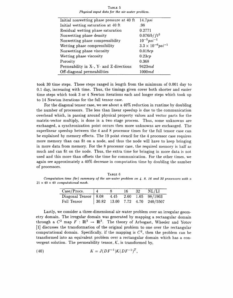
TABLE 5Physical input data for the air-water problem.

Initial non wetting phase pressure at 40 ftInitial wetting saturation at 40 ftResidual wetting phase saturationNonwetting phase densityNonwetting phase compressibilityWetting phase compressibilityNonwetting phase viscosityWetting phase viscosityPorosityPermeability in X-, Y- and Z-directionsOff-diagonal permeabilities

14.7psi.980.27710.076Ib/ ft31O-5psi-1

3.3 X 1O-6psi-1

0.018cp0.23cp0.3689423md1000md

took 30 time steps. These steps ranged in length from the minimum of 0.001 day to0.1 day, increasing with time. Thus, the timings given cover both shorter and easiertime steps which took 3 or 4 Newton iterations each and longer steps which took upto 14 Newton iterations for the full tensor case.

For the diagonal tensor case, we see about a 40% reduction in runtime by doublingthe number of processors. The less than linear speedup is due to the communicationoverhead which, in passing around physical property values and vector parts for thematrix-vector multiply, is done in a two stage process. Thus, some unknowns areexchanged, a synchronization point occurs then more unknowns are exchanged. Thesuperlinear speedup between the 4 and 8 processor times for the full tensor case canbe explained by memory effects. The 19 point stencil for the 4 processor case requiresmore memory than can fit on a node, and thus the node will have to keep bringingin more data from memory. For the 8 processor case, the required memory is half asmuch and can fit on the node. Thus, the extra time for bringing in more data is notused and this more than offsets the time for communication. For the other times. weagain see approximately a 40% decrease in computation time by doubling the numberof processors.

TABLE 6Computation time (hr) summary of the air-water problem on 4. 8. 16 and 32 proces.sol'S with a

21 x 40 x 40 computational mesh.

Case/Procs.Diagonal TensorFull Tensor

48.0830.82

84.4513.00

162.607.72

321.654.70

NL/LI98/1903240/5507

Lastly, we consider a three-dimensional air-water problem over an irregular geom-etry domain. The irregular domain was generated by mapping a rectangular domainthrough a. C2 map F : m.3 --+ IR3• The theory of Arbogast, Wheeler and Yotov[1] discusses the transformation of the original problem to one over the rectangularcomputational domain. Specifically, if the mapping is C2, then the problem can betransformed into an equivalent problem over a rectangular domain which has a con-vergent solution. The permeability tensor, K, is transformed by,

(40)

where DF is the Jacobian of the map, F, and J is the determinant of DF. The result-ing permeability tensor on the rectangular domain will be full even in the case thatthe original on the irregular domain is diagonal. Furthermore, the time derivative andsource terms are multiplied by J. Applying these transformations allows computationover a regular grid.

Physical data for the irregular domain is the same as that given above for theair-water problem except that we consider a larger domain,

o ::; x ::;20ft,

o ::; y ::; 100ft,o ::; :: ::; 100ft,

and a larger injection region of 1Gft x 16ft at the domain top.· The domain wasdivided into a 10 x 20 x 20 wllIputation grid, giving 4000 gridblocks.

Figures 10 and 11 give contour plots of the water saturation after 5 and 15 simu-lation days, respectively. W<,S(l(' t hat the water moves outward and slowly downwardfrom the injection zone. Aft pr 1:) da~·s. a significant amount of water has flowed tothe bottom and started to pool at t hf' base of the domain.

Water Saturation at 5 Days

Water Saturation

.- 0340.310.28

i:'J~'~:~~.

"." 0.19

0.t60.13

FIG. 10. Contour plot of water saturation for the irregulm' domain air-water problem after 5simulation days.

8. Conclusions and further work. We have described a fully implicit paralleltwo-phase flow simulator that incorporates new advances in the solution of large scalenonlinear problems. Our approach consists of an inexact Newton procedure with aKrylov subspace method as the inner iteration. In order to achieve robustness wehave implemented a two-stage IMPES type preconditioner that uses line correctionand an inner GMRES iteration for solving the pressure system. This inner-outerprocedure has been shown to be effective in handling ill-conditioned linear systemsarising from large time steps or problems with severe physical conditions. We alsoinclude a dynamic forcing term selection as well as line-search globalization for the

Water Saturation at 15 Days

Water Saturation

H 0.34'~~: 0.3t

--J 0.28i 0.25

0.220.19O.tS0.t3

FIG. 11. Contour plot of water saturation for the irregular domain air-water problem after 15simulation days.

Newton method. The former provides an efficient mechanism to avoid unnecessarylinear iterations and the latter increases the robustness of the Newton method.

We have employed the expanded mixed finite element method in order to simulateheterogeneities present in the physical domain. Furthermore, this method allows forthe modeling of general domain geometries. In order to add flexibility to our numericalmodel we have implemented several types of boundary conditions.

The two-stage preconditioner has been proven to be robust but further work isneeded to accelerate its performance. The authors believe that cheaper and even morerobust preconditioners should be developed for solving the pressure system. A moreaccurate way of collapsing the problem through line correction or symmetrization ofthe pressure system seems to be an immediate concern. Recent research indica.testhat incorporation of partial information from the decoupled saturation variables cansignificantly reduce the number of steps required for the linear Newton equation solver[37]. In this case, research is being done to incorporate ways of cutting the costassociated with GMRES and taking advantage of the Krylov information generated(see [36]). Also, strategies to "freeze" parts of the two-stage preconditioner for severaltime steps could be appealing in combination with polyalgorithmic approaches (seee.g., [23]).

With respect to the nonlinear iteration, current research is focused on the useof multilevel techniques for solving nonlinear parabolic equations. These techniques,based on the ideas of Xu [49], require the solution of the nonlinear problem on acoarse grid of size H. The problem is then projected to a fine grid of size h < < Handlinearized about the coarse grid solution. The linear fine grid problem is then solved.This procedure can be repeated for any number of grids where each fine grid problemis like a Newton step for the original nonlinear problem. Asymptotic error estimatesfor this technique applied to cell-centered finite differences for a nonlinear parabolicequation are derived in [17].

Finally, we encourage the use of these ideas for three phases and multicomponent

systems. The inclusion of more features into the simulator will certainly generatefurther insights and enhancements to the model tha.t we have proposed here.

Acknowledgments. The authors wish to thank John Wallis and Homer Walkerfor their valuable advice in the implementation of the solver.

REFERENCES

[1] T. ARBOGAST, M. F. WHEELER, AND I. YOTOV, LogicallyrectangularmixedmethodsfOl'ground-water flow and transport on general geometry, Dept. Compo Appl. Math. TR94-03. RiceUniversity, Houston, TX 77251. Jan. 1994.

[2] -, Mixed finite elements for elliptic problems with tensor coefficients as cell-centered finitedifferences, Dept. Compo Appl. Math. TR95-06. Rice University. Houston, TX 77251. mar1995. To appear SIAM J. Numer. Anal.. 1997.

[3] O. AXELSSOl\", Iterative Solution Methods, Cambridge University Press. 1994.[4] K. AZIZ AND A. SETHARI, Petroleum Reservoir Simulation, Applied Science Publisher. 1983.[5] R. BARRET, M. BERRY, T. CHAN, J. DEMMEL, J. DONATO, J. DONGARRA, V. EIJKHOL'T,

R. POZO, C. ROMINE, AND H. VAl\"DER VORST. Templates for the Solution of Linear Sys-tems: Building Blocks for Iterative Methods, SIAM, Philadelphia, 1994.

[6] J. BEAR, Dynamics of Fluids in Porous Media, Elsevier, New York, 1972.[7] G. BEHlE AND P. FORSYTH, Incomplete factorization methods for fully implicit simulation of

enhanced oil recovery, SIAM J. Sci. Statist. Comput., 5 (1984), pp. 543-561.[8] G. BEHlE Al\"DP. VINSOME, Block iterative methods for fully implicit reservoir simulation, Soc.

of Pet. Eng. J., (1982), pp. 658-668.[9] P. BJORSTAD, \IV. C. JR., Al\"D E. GROSSE, Parallel domain decomposition applied to coupled

transport equations, in Seventh International Conference on Domain Decomposition Methodsfor Scientific Computing, D. Keyes and J. Xu, eds .. Como, Italy. 1993, American Mathe-matical Society.

[10] P. BROWl\" Al\"D Y. SAAD, Hybrid Krylov methods for nonlinear systems of equations. SIAM J.Sci. Statist.. Comput .. 11 (1990), pp. 450-481.

[11] P. N. BROWl\", A. HIl\"DMARSH, Al\"D L. PETZOLD, Using Krylov methods in the solution oflarge-scale differential-algebraic systems, SIAM J. Sci. Comput .. 15 (1994), pp. 1467-1488.

[12] P. N. BROWl\"AND Y. SAAD, Convergence theory of nonlinear Netwon-f( rylov algorithms, SIAMJ. Optim., 4 (1994). pp. 297-330.

[13] X.-C. CAl, W. GROPP. D. KEYES, Al\"DM. TIDRIRI, Newton-Krylov-Schwarz methods in CFD,in International Workshop on the Navier-Stokes Equations, R. Rannacher, ed., Braun-schwieg, 1994, Notes in Numerical Fluid Mechanics. Vieweg Verlag.

[14] M. A. CELIA AND P. BIl\"l\"Il\"G,A mass conservative numerical solution for two-phase flow inporous media with application to unsaturated flow, Water Resources Research. 28 (1992).pp. 2819-2828.

[15] T. CHAl\" Al\"D T. MATHEW, Domain decomposition algorithms. in Acta Numerica, CambridgeUniversity Press, New York. 1994, pp. 61-143.

[16] G. CHAVEl\"TAl\"DJ. JAFFRE, Mathematical models and finite elements for reservoir simulation.North-Holland. Amsterdam, 1986.

[17] C. N. DAWSOl\", C. A. SAl\" SOL'CIE, AND M. F. WHEELER, A two-grid finite difference schemefor nonlinear parabolic equations, Dept. Compo Appl. Math. TR95-32, Rice Universit.y, Hous-ton, TX 77251, Oct. 1995.

[18] J. DEl\"DY, Multigrid methods for three dimensional petroleum reservoir simulation, in TenthSPE Symposium on Reservoir Simulation, SPE paper no. 18409. Houston, Texas, 1989.

[19] J. E. DEl\"l\"ISAl\"D R. B. SCHl\"ABEL, Numerical methods for unconstrained optimization andnonlinear equations, Prentice-Hall, Englewood Cliffs, New Jersey, 1983.

[20] L. J. DCRLOVSKY, Numerical calculation of equivalent grid block permeability tensors for het-erogeneous porous media, Water Resources Research. 27 (1991), pp. 699-708.

[21] S. EISENSTAT AND H. WALKER, Globally convergent inexact Newton methods, SIAM J. Opti-mization, 4 (1994), pp. 393-422.

[22] -, Choosing the forcing terms in an inexact Newton method, SIAM J. Sci. Comp., 17 (1996),pp. 16-32.

[23] A. ER!\, V. GIOVA!\GIGLI, D. KEYES. A!\D M. D. SMOOKE, Towards polyalgorithmic linearsystem solvers for nonlinear elliptic problems. SIAM J. Sci. Comput., 15 (I994), pp. 681-703.

[24] R. EWI!\G, The mathematics of reservoir simulation, in Frontiers in Applied Mathemat.ics,SIAM, Philadelphia, 1983.

[25] P. FORSYTH AND P. SAMMO!\, Practical considerations for adaptive implicit methods in reservoirsimulation, J. of Compo Physics, 62 (1986), pp. 265-281.

[26] P. A. FORSYTH, Y. S. Wt:, A!\D K. PRUESS. Robust numerical methods for saturated-unsaturatedflow with dry initial conditions in heterogeneous media, Advances in Water Resources, 18(1995), pp. 25-38.

[27] R. A. FREEZE A!\D J. A. CHERRY, Groundwater, Prentice Hall, Inc., New Jersey, 1979.[28] R. FREt:!\D, G. GOLUB, AND N. M. NACHTIGAL, Iterative solution of linear systems, in Acta

Numerica, Cambridge University Press, New York, 1991, pp. 57-100.[29] G. GOLUB AND C. V. LOAN, Matrix Computations. John Hopkins University Press, 1989.[30] S. GOMEZ A!\D J. MORALES, Performance of Chebyshev iterative method, GMRES and OR-

THOMIN on a set of oil reservoir simulation problems, in Mathematics for Large ScaleComputing, In J.C. Diaz. New York, Basel, 1989, pp. 265-295.

[31] R. HANBY, D. SYLVESTER, AND J. CHEW, A comparison of coupled and segregated iterativesolution techniques for incompressible swirling flow, Tech. Report TR94-246, University ofManchester. 1994.

[32] V. HAROt:TUNIAN, M. ENGELMAN, AND I. HASBANI, Segregated finite element algol'ithms forthe numerical solution of large-scale incomprenssible flow problems. Int. J. Numer. MethodsFluids, 17 (1993), pp. 323-348.

[33] M. T. VAN GENUCHTE!\, A closed form equation for predicting the hydraulic conductivity ofunsaturated soils, Soil Sci. Soc. Am. J., 44 (1980), pp. 892-898.

[34] C. KELLEY. Iterative methods for linear and nonlinear equations, in Frontiers in Applied Math-ematics, SIAM, Philadelphia, 1995.

[35] T. KERKHOVE!\ A!\D Y. SAAD, On acceleration methods for coupled nonlinear elliptic problems.Numer. Math., 60 (1992), pp. 525-548.

[36] H. KLIE. M. RAME, A!\D M. WHEELER. Krylov-secant methods for solving systems of nonlinearequations, Tech. Report TR95-27, Dept. of Computational and Applied Mathemat.ics, RiceUniversity, 1995.

[37] -, Two-stage preconditioners for inexact Newton methods in multi-phase reservoir simu-lation, Tech. Report CRPC- TR96641. Center of Research on Parallel Computation, RiceUniversity, 1996.

[38] V. Kt:MAR, A. GRAMA, A. Gt:PTA, A!\D G. KARYPIS, Introduction to Parallel Computing:Design and Analysis of Algorithms, The Benjamin/Cummings Publishing Company, Inc ..1994.

[39] C. MATTAX A!\D R. DALTO!\, Reservoir Simulation. vol. 13, SPE-Monograph Series. Richardson.TX,1990.

[40] J. NEDELEC, Mixed finite elements in IR3, Numer. Math., 35 (1980), pp. 315-341.[41] D. W. PEACEMA!\, Fundamentals of numerical reservoir simulation, Elsevier, 1977.[42] P. A. RAVIART AND J. M. THOMAS, A mixed finite element method for second order elliptic prob-

lems, in Mathematical Aspects of Finite Element Methods: Lecture Notes in Mathematics606, I. Galligani and E. Magenes, eds., Berlin, 1977, Springer-Verlag, pp. 292-315.

[43] R. TEIGLA!\D A!\D G. FLADMARK, Cell centered multigrid methods in porous media flow, inMultigrid methods III : proceedings of the 3rd European Multigrid Conference. BirkhauserVerlag, 1991.

[44] S. Tt:REK, On discrete projection methods for the incompressible Navier-Stokes equations. Inpreparation, 1994.

[45] J. WALLIS, Two-step preconditioning. Private Communication, 1994.[46] J. WATTS, A method of improving line succesive overrelaxation in anisotropic problems-a theo-

retical analysis. Soc. of Pet. Eng. J., (1973), pp. 105-118.[47] J. \VHEELER A!\D R. SMITH, Reservoir simulation on a hypercube, in 64th Annual Technical

Conference and Exhibition of the Society of Petroleum Engineers, SPE paper no. 19804,San Antonio, Texas, 1989.

[48] L. WIGTO!\, D. Yu, A!\D N. YOt:NG, GMRES acceleration of computational fluid dynamicscodes, in Proceedings 1985 AIAA Conference, Denver, CO, 1985.

[49] J. XU, Two-grid finite element discretizations for nonlinear elliptic equations, Dept. of Mat.h-