A Parallel Linear Solver for Block Circulant Linear Systems with Applications to Acoustics

Suzanne Shontz, University of Kansas Ken Czuprynski, University of Iowa

John Fahnline, Penn State

EECS 739: Parallel Scientific ComputingUniversity of Kansas

January 23, 2019

MOTIVATION

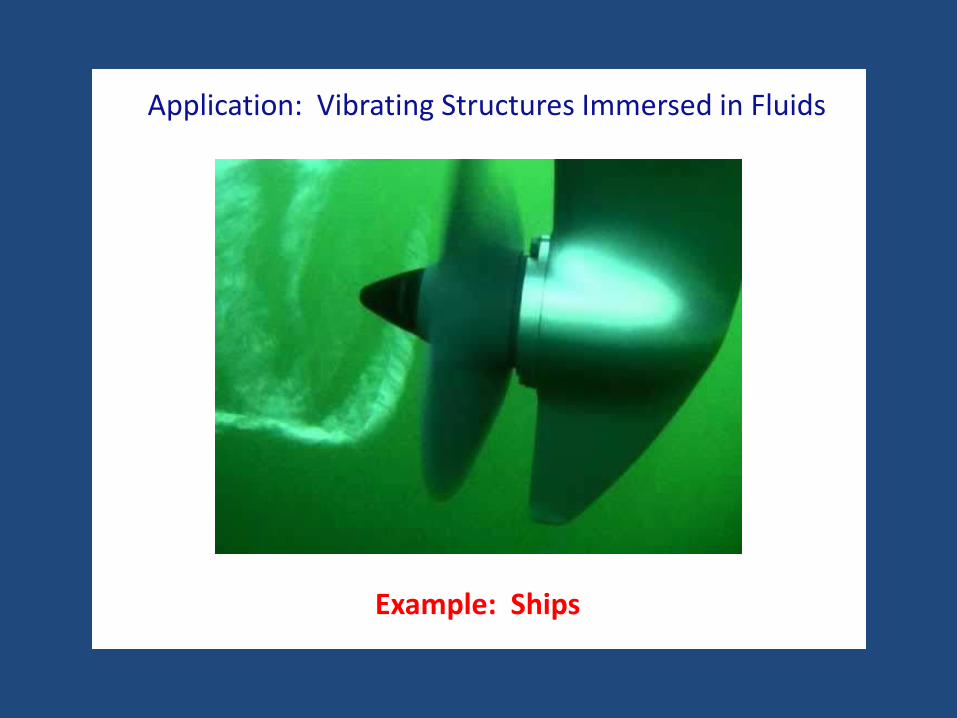
Application: Vibrating Structures Immersed in Fluids

Example: Ships

Example: UAVs

Example: Planes

Example: Blood Pumps

Example: Reactors

Examples of Rotationally Symmetric Boundary Surfaces

Real-world applications: propellers, wind turbines, etcetera

THE PROBLEM

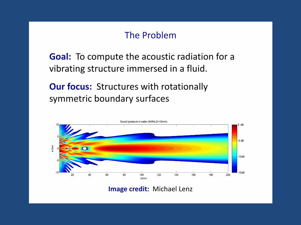
The Problem

Goal: To compute the acoustic radiation for a vibrating structure immersed in a fluid.

Our focus: Structures with rotationally symmetric boundary surfaces

Image credit: Michael Lenz

Parallel Linear Solver for Acoustic Problems with Rotationally Symmetric Boundary Surfaces

Context: Vibrating structure immersed in fluid. Acoustic analysis using boundary element method. Coupled to a finite element method for the structural analysis. We focus on the boundary element part of the calculation.

Goal: Solve block circulant linear systems to compute acoustic radiation of vibrating structure with rotationally symmetric boundary surface.

Approach: Parallel linear solver for distributed memory machines based on known inversion formula for block circulantmatrices.

THE BOUNDARY ELEMENT METHOD (BEM)

Boundary Element Method

The boundary element method (BEM) is a numerical method for solving linear partial differential equations (PDEs).

In particular, the BEM is a solution method for solving boundary value problems (BVPs) formulated using a boundary integral formulation.

Discretization: Only of the surface (not of the volume). Reduces dimension of problem by one.

BEM: Used on exterior domain problems and when greater accuracy is required.

We employ the boundary element method to obtain the linear system of equations.

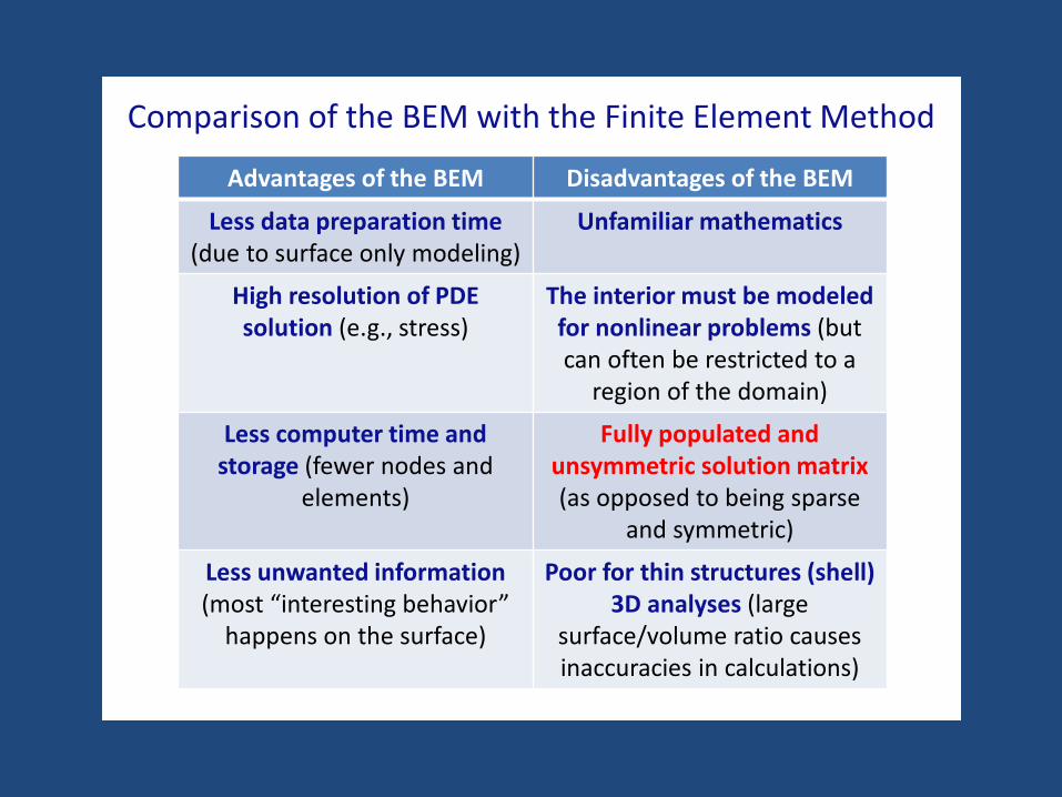
Comparison of the BEM with the Finite Element Method

Advantages of the BEM Disadvantages of the BEM

Less data preparation time (due to surface only modeling)

Unfamiliar mathematics

High resolution of PDE solution (e.g., stress)

The interior must be modeled for nonlinear problems (but can often be restricted to a

region of the domain)

Less computer time and storage (fewer nodes and

elements)

Fully populated and unsymmetric solution matrix (as opposed to being sparse

and symmetric)

Less unwanted information (most “interesting behavior”

happens on the surface)

Poor for thin structures (shell) 3D analyses (large

surface/volume ratio causes inaccuracies in calculations)

BLOCK CIRCULANT MATRICESVIA THE BOUNDARY ELEMENT

METHOD

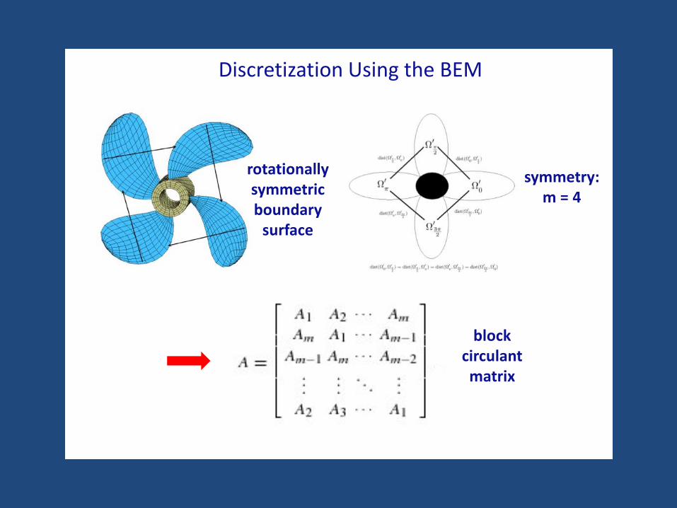
Discretization Using the BEM

rotationallysymmetricboundary

surface

symmetry:m = 4

blockcirculantmatrix

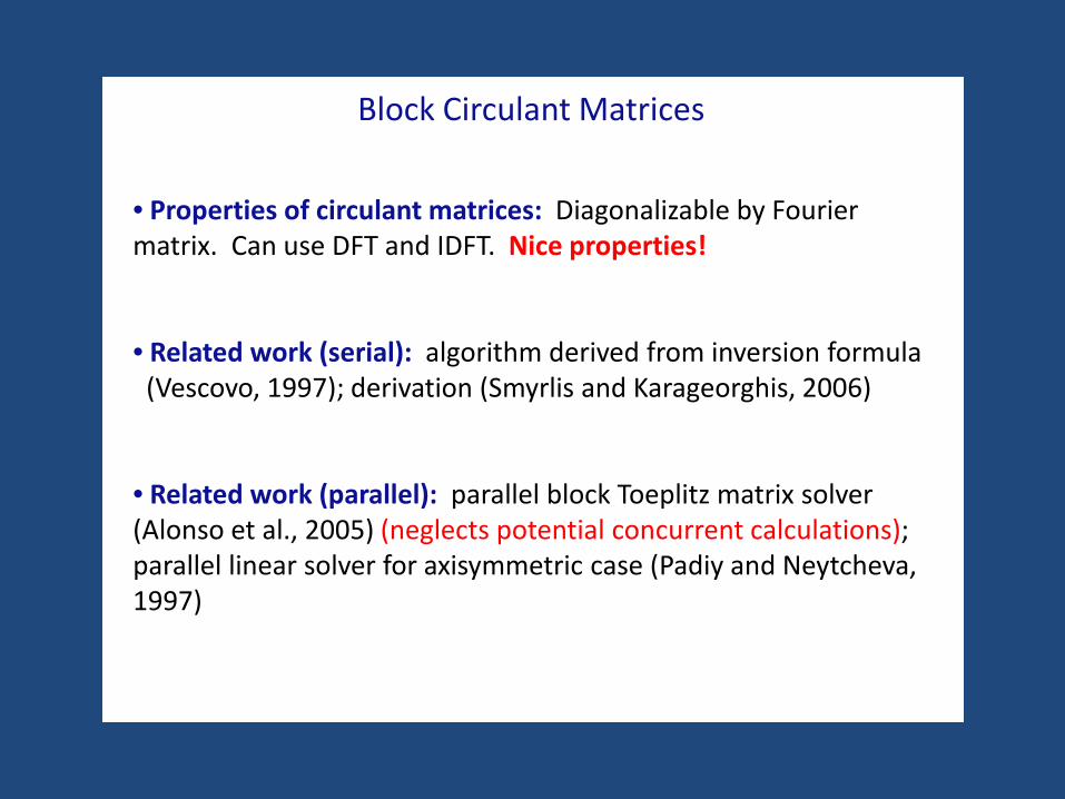
Block Circulant Matrices

• Properties of circulant matrices: Diagonalizable by Fourier matrix. Can use DFT and IDFT. Nice properties!

• Related work (serial): algorithm derived from inversion formula (Vescovo, 1997); derivation (Smyrlis and Karageorghis, 2006)

• Related work (parallel): parallel block Toeplitz matrix solver (Alonso et al., 2005) (neglects potential concurrent calculations); parallel linear solver for axisymmetric case (Padiy and Neytcheva, 1997)

MATHEMATICAL FORMULATION OF LINEAR

SYSTEM OF EQUATIONS

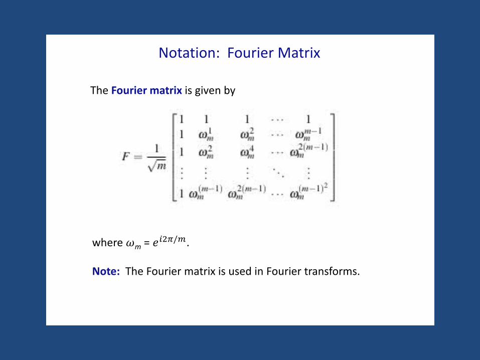
Notation: Fourier Matrix

The Fourier matrix is given by

where 𝜔𝜔m = 𝑒𝑒𝑖𝑖𝑖𝜋𝜋/𝑚𝑚.

Note: The Fourier matrix is used in Fourier transforms.

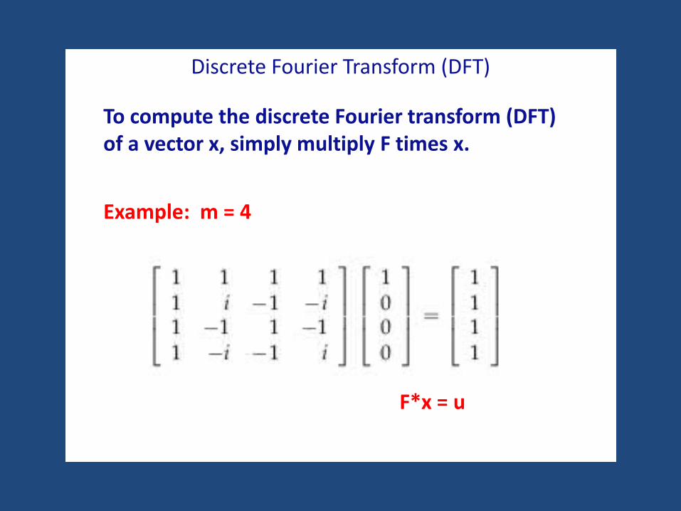
Discrete Fourier Transform (DFT)

To compute the discrete Fourier transform (DFT) of a vector x, simply multiply F times x.

Example: m = 4

F*x = u

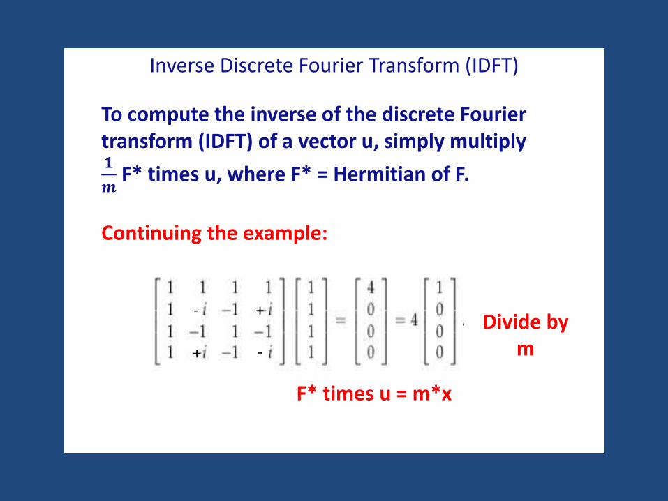
Inverse Discrete Fourier Transform (IDFT)

To compute the inverse of the discrete Fourier transform (IDFT) of a vector u, simply multiply 𝟏𝟏𝒎𝒎

F* times u, where F* = Hermitian of F.

Continuing the example:

Divide bym

F* times u = m*x

- +

+ -

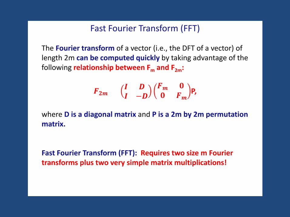
Fast Fourier Transform (FFT)

The Fourier transform of a vector (i.e., the DFT of a vector) of length 2m can be computed quickly by taking advantage of the following relationship between Fm and F2m:

𝑭𝑭𝟐𝟐𝒎𝒎 = 𝑰𝑰 𝑫𝑫𝑰𝑰 −𝑫𝑫

𝑭𝑭𝒎𝒎 𝟎𝟎𝟎𝟎 𝑭𝑭𝒎𝒎

P,

where D is a diagonal matrix and P is a 2m by 2m permutation matrix.

Fast Fourier Transform (FFT): Requires two size m Fourier transforms plus two very simple matrix multiplications!

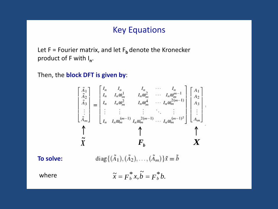
Key Equations

Let F = Fourier matrix, and let Fb denote the Kroneckerproduct of F with In.

Then, the block DFT is given by:

To solve:

where

X~ XbF

.*~,*~ bFbxFx bb ==

SERIAL ALGORITHM

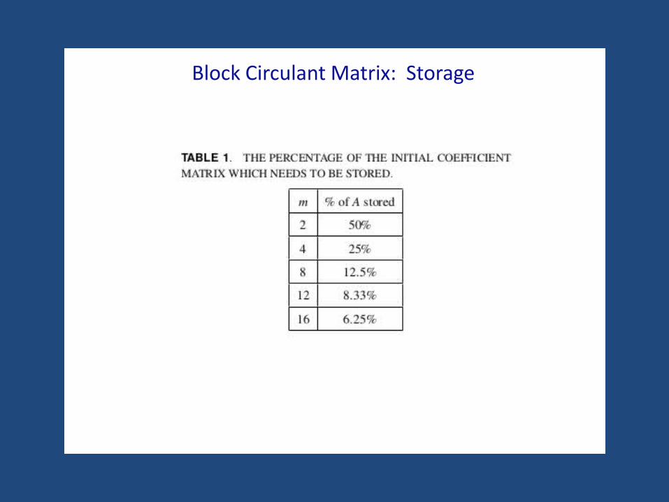
Block Circulant Matrix: Storage

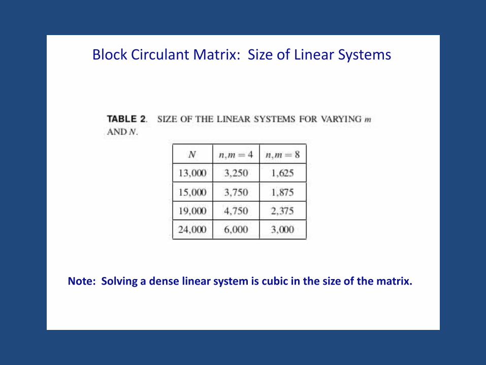
Block Circulant Matrix: Size of Linear Systems

Note: Solving a dense linear system is cubic in the size of the matrix.

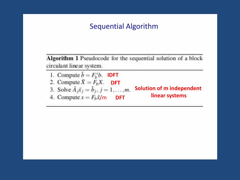
Sequential Algorithm

IDFTDFT

Solution of m independent linear systemsDFT/m

PARALLEL ALGORITHM

How to Parallelize the Algorithm?

Recall, we are interested in solving

where

.*~,*~ bFbxFx bb ==

m independent

linear systemsto solve!

Ideas?

Block DFT Algorithm

• A block DFT calculation is the basis for our parallel algorithm.

• This demonstrates improved robustness (over use of the FFT) and allows for any boundary surface to be input.

DFT Computation

This generalizes to the case when P > m.

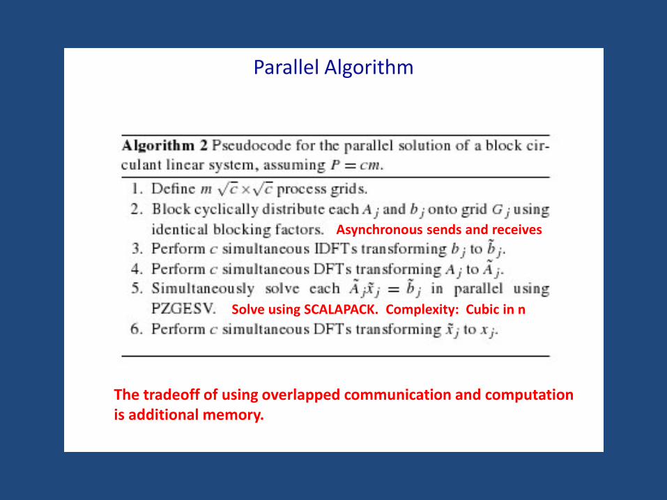
Parallel Algorithm

Solve using SCALAPACK. Complexity: Cubic in n

Asynchronous sends and receives.

The tradeoff of using overlapped communication and computationis additional memory.

NUMERICAL EXPERIMENTS

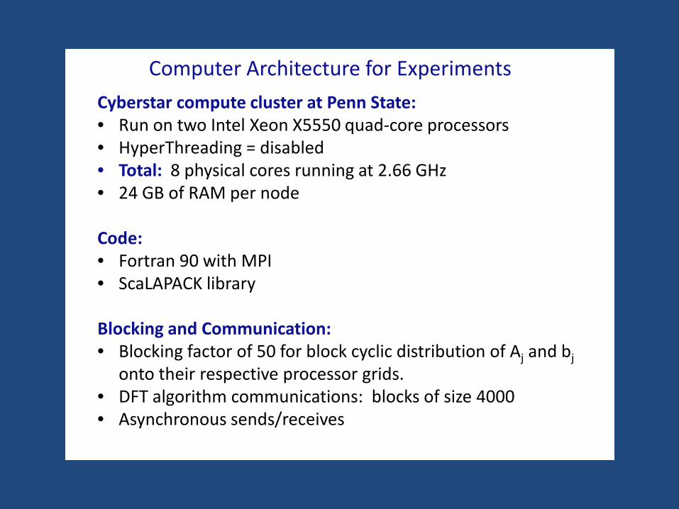
Computer Architecture for ExperimentsCyberstar compute cluster at Penn State:• Run on two Intel Xeon X5550 quad-core processors• HyperThreading = disabled• Total: 8 physical cores running at 2.66 GHz• 24 GB of RAM per node

Code:• Fortran 90 with MPI• ScaLAPACK library

Blocking and Communication:• Blocking factor of 50 for block cyclic distribution of Aj and bj

onto their respective processor grids.• DFT algorithm communications: blocks of size 4000• Asynchronous sends/receives

Metrics for Experiments

• Runtime = wall clock time of parallel algorithm= Tp

• Speedup = how much faster is the parallel algorithm than the serial algorithm = S = Ts/Tp

• Efficiency = E = S/P

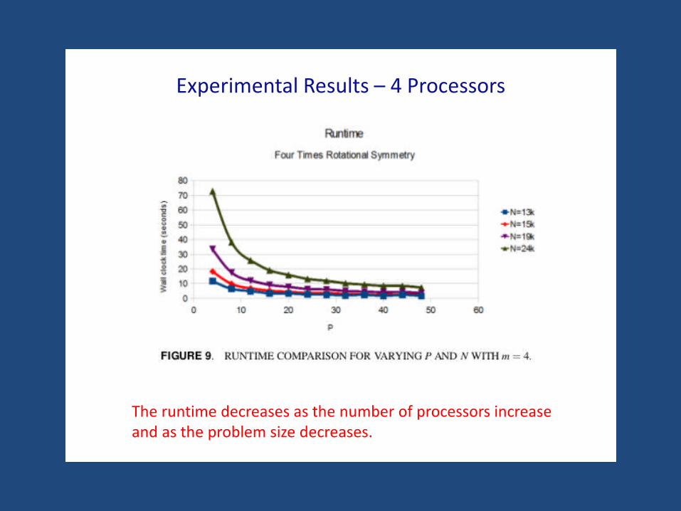
Experimental Results – 4 Processors

The runtime decreases as the number of processors increaseand as the problem size decreases.

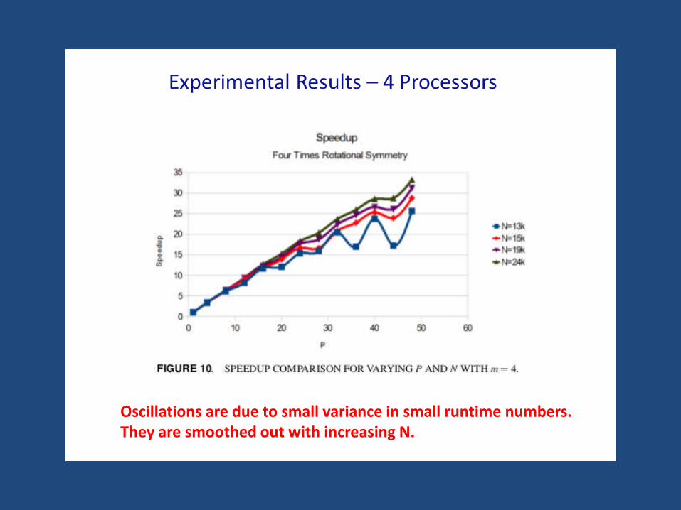
Oscillations are due to small variance in small runtime numbers.They are smoothed out with increasing N.

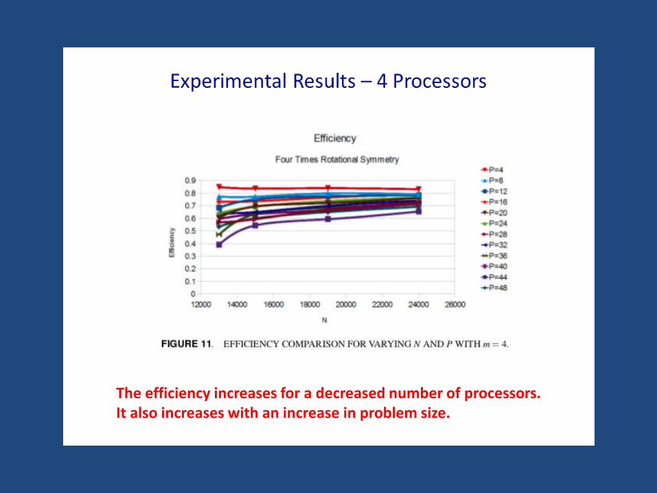
The efficiency increases for a decreased number of processors. It also increases with an increase in problem size.

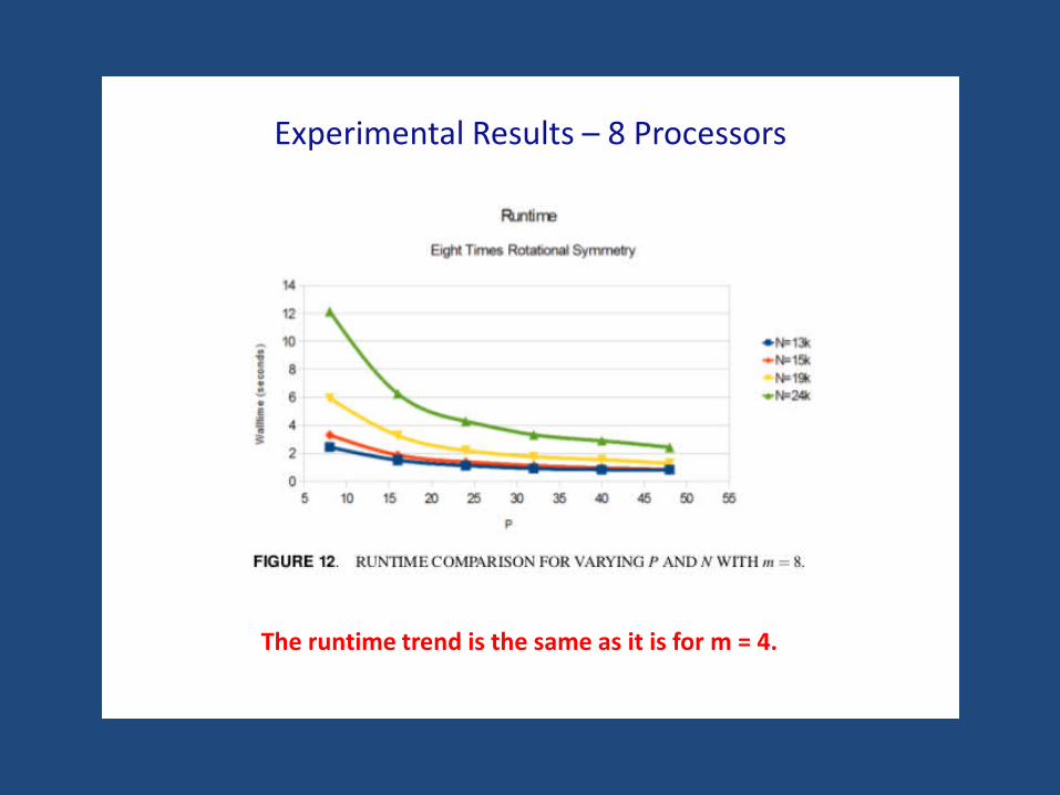
Experimental Results – 8 Processors

The runtime trend is the same as it is for m = 4.

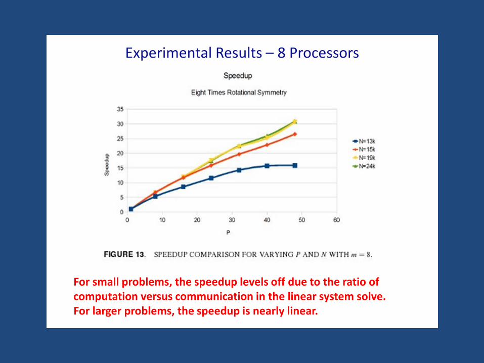
Experimental Results – 8 Processors

For small problems, the speedup levels off due to the ratio of computation versus communication in the linear system solve. For larger problems, the speedup is nearly linear.

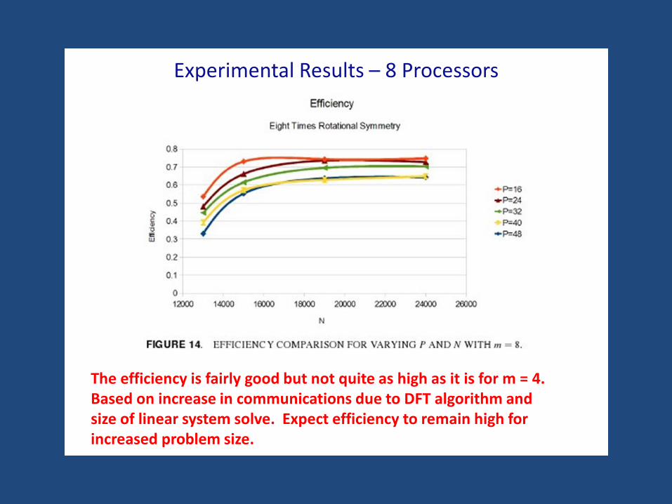
Experimental Results – 8 Processors

The efficiency is fairly good but not quite as high as it is for m = 4.Based on increase in communications due to DFT algorithm and size of linear system solve. Expect efficiency to remain high for increased problem size.

CONCLUSIONS

Conclusions• We have proposed a parallel algorithm for solution of block

circulant linear systems. Arise from acoustic radiation problems with rotationally symmetric boundary surfaces.

• Based on block DFTs (more robust) and have embarrassingly parallel nature based on ScaLAPACK’s required data distributions.

• Reduced memory requirement by exploiting block circulantstructure.

• Achieved near linear speedup for varying problem size, linear speedup for large N. Efficiency increases with problem size.

• Can solve larger/higher frequency acoustic radiation problems.

Reference

K.D. Czuprynski, J. Fahnline, and S.M. Shontz, Parallel boundary element solutions of block circulant linear systems for acoustic radiation problems with rotationally symmetric boundary surfaces, Proc. of the Internoise 2012/ASME NCAD Meeting, August 2012.

Acknowledgements

This work is based on the M.S. Thesis of Ken Czuprynski in addition to our Internoise 2012 paper.

Computing Infrastructure:• NSF grant OCI-0821527

Research Funding:• Penn State Applied research Laboratory’s Walker

Assistantship Program (Czuprynski)• NSF Grant CNS-0720749 (Shontz)• NSF CAREER Award OCI-1054459 (Shontz)