A parallel matrix-free framework for frequency-domainseismic modelling, imaging and inversion in Matlab

Tristan van Leeuwen

Dept. of Earth and Ocean sciences, University of British Columbia, 6339 stores road, Vancouver, BC,Canada, V6T 1Z4

Abstract

I present a parallel matrix-free framework for frequency-domain seismic modeling,imaging and inversion. The framework provides basic building blocks for designingand testing optimization-based formulations of both linear and non-linear seismic in-verse problems. By overloading standard linear-algebra operations, such as matrix-vector multiplications, standard optimization packages can be used to work with thecode without any modification. This leads to a scalable testbed on which new methodscan be rapidly prototyped and tested on medium-sized 2D problems. I present somenumerical examples on both linear and non-linear seismic inverse problems.

Keywords: Seismic imaging, optimization, Matlab, object-oriented programming

1. Introduction

Seismic data are a rich source of information on the subsurface. Large amountsof data are acquired for both academic and industrial purposes, either through activeexperiments or by recording earth-quake responses. Over the years many different for-mulations and algorithms have been proposed to estimate subsurface properties basedon such data. Over the past two decades these algorithms have come to rely heavilyon high-performance computing. A successful seismic inversion framework needs tocombine a modeling engine to solve a wave-equation (e.g., finite differences or finiteelements), (non-) linear optimization algorithms and facilitate i/o of large amounts ofdata and the corresponding meta data. Due to the large scale of typical problems, acomputer code that implements these algorithms and concepts has to be extremely ef-ficient, scalable and robust. On the other hand, the interdisciplinary nature of suchprojects requires that experts from different fields can contribute to the code. Needlessto say, some form of unit-testing needs to be incorporated to facilitate de-bugging. Thechallenge is in meeting these, seemingly mutually exclusive, requirements.

A necessary (but not sufficient) condition is that the basic building blocks of thecode, such as the modeling operator, its Jacobian and their basic operations (forwardmodeling, action of the Jacobian and its adjoint) are exposed. This allows the unitsto be tested separately and re-used for different purposes. Then, these building blocksshould be cast in pre-defined classes, such as (non-) linear operators and functionals.

Preprint submitted to Elsevier July 3, 2012

This allows us to have our code reflect the underlying mathematical principles andserves a bridge to existing code. We do not have to sacrifice efficiency when followingthese principles because the individual blocks can still contain highly optimized code.

An added bonus of such a framework is that it allows for rapid prototyping andincreases reproducibility. Because the separate building blocks expose the underlyingmathematics, it should be relatively straightforward to understand and implement thealgorithm using a different modeling kernel (given that is also exposes the basic func-tionality as described above). Unit tests can ensure that any given implementation iscorrect.

For further reading on this design philosophy I refer the reader to [1] and [2] whoillustrates the approach for time-stepping codes and C++. A few existing librariesthat facilitate such approaches to various degrees are PETSC [3], Trilinos [4], the RiceVector Library [5] and SPOT [6].

Framework

To illustrate the design principles sketched above, I present a parallel matrix-freeframework for frequency-domain wavefield modelling, imaging and inversion in Mat-lab. The basic building blocks of the framework are the finite-difference modelingoperator d = F(m) that maps a model of the subsurface m to the observed data d, andits Jacobian ∇F(m), implemented as matrix-free linear operator. Using these buildingblocks, we can formulate algorithms to solve the basic inverse problem

for given observations dobs, find a model m for which the predicteddata F(m) fits the observed data.

In particular, I will focus on optimization-based formulations of this problem

minm

W(F(m),dobs), (1)

where W measures the misfit between the observed and predicted data (e.g., for non-linear least-squares W(·, ·) = || · − · ||22).

Matlab code

The Matlab code is available for academic purposes. The code to reproduce theexamples presented in this paper is also included. See https://www.slim.eos.ubc.ca/releases for download instructions.

Outline

First, I discuss the modeling kernel, which consists of the forward modeling op-erator and its Jacobian. Then I show how to use a framework for matrix-free linearalgebra in Matlab to implement functionality needed for various imaging and inversionpurposes. I discuss how the different units of code should be tested and finally, givesome numerical examples on both linear and non-linear seismic inverse problems.

2

Notation• x - lowercase, italic symbols denote scalars

• x - lowercase, boldface symbols denotes column vectors whose elements aredenoted as xi

• A - capital italic symbols denote matrices or linear operators and ·† denotes their(conjugate) transpose or adjoint.

• vec(·) denotes vectorization, vec−1(·) denotes reshaping into the original size.

• diag(·) when applied to a matrix extracts the diagonal from a matrix, when ap-plied to a vector constructs a diagonal matrix.

• F(·) - capital sans-serif symbols denote non-linear operators, and ∇F denotes theJacobian.

• f(·) - lower case sans-serif symbols denote functions and ∇f denotes the gradient.

• S - curly capital letters denote sets/lattices/grids.

2. Modeling

Wave-propagation in the earth is assumed to obey a scalar Helmholtz equation:

Aω(m)u = q. (2)

Here Aω(m) is the discretized Helmholtz operator ω2m + ∇2 – with some form ofabsorbing boundary conditions to simulate an infinite domain – for frequency ω andsquared slowness m in seconds2/meters2, u is the wavefield and q represents the source.

GridsI define 4 distinct grids that are used during the computations:

• The physical grid G. This grid represents the region of interest. The mediumparamerer m is discretized on this grid.

• The computational grid C, which is an extension of the physical grid. TheHelmholtz operator is discretized on this grid. The extended area is used forthe absorbing boundary conditions.

• The source grid S. This grid is a subset of the physical grid and is used to definethe source functions.

• The receiver grid R. This grid is a subset of the physical grid and is used todefine the receiver array.

Figure 1 illustrates the different grids. Quantities are mapped from one grid to theother via interpolation or padding:

• PX is a 2D interpolation operator that interpolates from C to X,

• EX padds the input, defined on grid X with its boundary values to the computa-tional grid C.

3

Source representationI use adjoint interpolation to represent point-sources. This ensures that the point-

source will behave like a discretized delta function to some extent. Consider the fol-lowing 1D example. The source-grid is a single point S = { 12 } while the computationalgrid is given by C = {0, 1

5 ,25 ,

35 ,

45 , 1}. Define the interpolation operator PS to inter-

polate from C to S. The source function on the source grid is a single scalar q = 1.The resulting source functions for linear, quadratic and cubic interpolation are shownin figure 2. For given polynomials pl = [0, 1

5 ,25 ,

35 ,

45 , 1]l, we want our discretized delta

function to satisfy

〈pl, PS†q〉C =(

12

)l, (3)

up to some order. We can write this requirement as 〈PCpl,q〉S = PCpl = ( 12 )l, from

which it follows that the order to which this requirement will be satisfied is determinedby the accuracy of the interpolation operator. A numerical verification is shown in table1.

Modeling operatorThe data for one frequency and source is obtained via

di j = PRAωi (EGm)−1PS†qi j. (4)

The modeling operator F solves (4) for several frequencies i = 1, . . . , n f and sourcesj = 1, . . . , ns and organizes the result in a vector.

Linearized modeling opertorThe Jacobian of the modeling operator, ∇F, for one source and frequency is given

by

∂di j

∂m= PRAωi (EGm)−1Gωi (m,ui j)EG, (5)

where ui j = Aωi (EGm)−1PS†qi j and Gω(m,u) =(∂Aωu∂m

). In practice, the Jacobian ma-

trix is never formed explicitly. Instead, its action is computed by solving 2 Helmholtzsystems per source and frequency.

Analytic solutionsFor some specific cases, analytic expressions exist for the Greens function. For a

constant medium with velocity c0 we have

u =ı

4H1

0(ωr/c0), (6)

where H10 is a Hankel function of the first kind and ri =

√(xi − xs)2 + (zi − zs)2.

For linearly increasing velocity c0 + αz, the analytic solution is given by [7]

u = Qν− 12(s), (7)

4

where Qµ is a Legendre function and ν = ı√

(ω/α)2 − 14 and

si = 1 +12

r2i

(zs + c0/α)(zi + c0/α).

3. Matrix-free framework

The (linearized) modeling operator is readily implemented in Matlab, but interac-tion with existing code, especially for linear operators, is not always straightforward.To facilitate incorporation of these blocks into exisisting code, I adopt the SPOT tool-box for matrix-free linear algebra [6]. This allows us, for example, to perform matrix-free matrix-vector products by overloading the Matlab multiplication operation. Fur-thermore, by insisting on a certain structure of our non-linear operators we can easilyadopt ideas form algorithmic differentiation to calculate derivatives of combinations ofsuch operators.

3.1. Linear operators

To illustrate the workings of SPOT, let us consider the Fourier transform. Thefollowing code fragment defines an operator that performs the Fourier transform on avector of length 1000 and performs a forward and inverse FFT on a random vector.

n = 1000; % length

A = opDFT(n); % define SPOT operator

x = randn(n,1); % random vector of length n

y = A∗x; % forward FFT

x = A'∗y; % inverse/adjoint FFT

Upon multiplying the operator Awith the vector x, Matlab will call the function A.multiply(x,1),wich in turn will perform the Fourier transform using the Matlab built-in functionfft. Similarly, when multiplying the adjoint with y, Matlab will call the functionA.multiply(x,-1), which in turn calls ifft.

Custom linear operators can be implemented in a similar manner by supplying afunction that performs forward and adjoint multiplication. This function can be directlywrapped into a standard SPOT operator using opFunction, or the user can definea custom SPOT operator using the opSpot class. The latter allows one to overloadother Matlab built-in functions, such as mldivide, mrdivide, display, norm etc.Composition and addition of operators is also supported. For example, C = A*B, whereA and B are SPOT operators, will return a spot operator that multiplies with B andsubsequently with A. The Kronecker product is supported via C = opKron(A,B). Aparallel extension of SPOT, pSPOT [8, 9] allows us to define linear operators that workon distributed arrays.

The linear operators can be tested for consistency via the dot-test

〈Ax, y〉 = 〈x, A†y〉, (8)

5

where y has to be in the range of A. Typically, one takes x to be a random vector andwe can generate y by acting on another random vector with A. The two should be thesame up to numerical precision.

3.2. Non-linear operatorsFor non-linear operators and functions I use the convection that they return their

output (vector or scalar) and the Jacobian or gradient. This structure makes it ex-tremely easy to implement complictated chains of such operations. Furthermore, indi-vidual components can be tested seperately to facilitate debugging. One popular wayof testing gradients is based on the Taylor series

f(x0 + hδx) = f(x0) + h〈∇f(x0), δx〉 + O(h2), (9)

where x0 and δx are suitable testvectors. Alternatively, we can use the Taylor series attwo different points

f(x2) − f(x1) ≈12〈∇f(x1) + ∇f(x2), x2 − x1〉 (10)

Simimarly, for the non-linear operators we have

F(x0 + hδx) = F(x0) + h∇F(x1)δx + O(h2). (11)

It is easily verified that the error decays with h as predicted.

4. Implementation and testing

The modeling operator is implemented as a Matlab function [d,J] = F(m,Q,model),where each column of the matrix Q represents a gridded source function, model is astruct that contains descriptions of the grids and specifies the frequencies. The outputis the data d and the Jacobian as a SPOT operator J, which calls the function output =DF(m,Q,input,flag,model) to compute the forward (flag=1) or adjoint (flag=-1)action of the Jacobian on the vector input.

I use a 9-point mixed-grid stencil [10] to discretize the Helmholtz operator and usea sponge boundary condition. The resulting sparse matrix is inverted for all right-hand-sides simultaneously using Matlab’s mldivide, which (for sparse matrices) is based onan LU decomposition. The loop over frequencies is done in parallel using the ParallelComputing Toolbox, as will be discussed later.

Other building blocks, like interpolation, basic i/o and optimization methods arepart of the package. A brief description can be found in the appendix.

Accuracy of the modeling codeThe modeling operator is tested against analytic solutions for constant and linearly

increasing velocity profiles v = v0 +αz. Figure 3 (a) shows the error for v0 = 2000 m/s,α = 0 1/s and a frequency of 10 Hz as a function of the gridspacing. A slice through thewavefield is shown in figure 3 (b). The analytical and numerical soltions for v0 = 2000m/s, α = 0.7 1/s and a frequency of 10 Hz is shown in figures 3 (c) and (d) respectively.

6

Accuracy of the Jacobian

The accuracy of the Jacobian is tested according to (11) for a constant velocity anda random perturbation. The resulting error is shown in figure 4.

Consistency of the Jacobian

The consistency of the Jacobian is tested with the dottest (cf. eq. 8). The result on10 random vectors is shown in table 2.

Scalability

The modelling code is parallelized over frequencies using Matlab’s Parallel Com-puting Toolbox. We use the Single Program Multiple Data (SPMD) functionality ofthis tool box to divide the computation over the available processors. The basic algo-rithm is as follows:

% distribute frequencies using standard distribution

freq = distributed(model.freq);

spmd

% define distribution of data array

codistr = ...

codistributor1d (2,[],[ nsrc∗nrec ,nfreq]);% get local frequencies

freqloc = getLocalPart(freq);

nfreqloc = length(freqloc);

% loop over local frequencies

for k = 1: nfreqloc

% solve Helmholtz equation for local ...

frequencies and store resulting data in ...

Dloc

end

% build distributed array from local parts

D = codistributed.build(Dloc ,codistr);

end

To test the performance of the parallelization, I compute data for a model of size1200 × 404, for 10 sources and 64 frequencies. The compute cluster consists of 36 IBMx3550 nodes, each with 2 quad core Intel 2.6Ghz CPUs, 16 GB RAM and a Volterra x4inter-processor network. We used 1 processor per node plus one master node (used byMatlab to manage the computation and not counted in the total number of CPUs used).The results for various numbers of CPUs are shown in table 3.

7

5. Examples

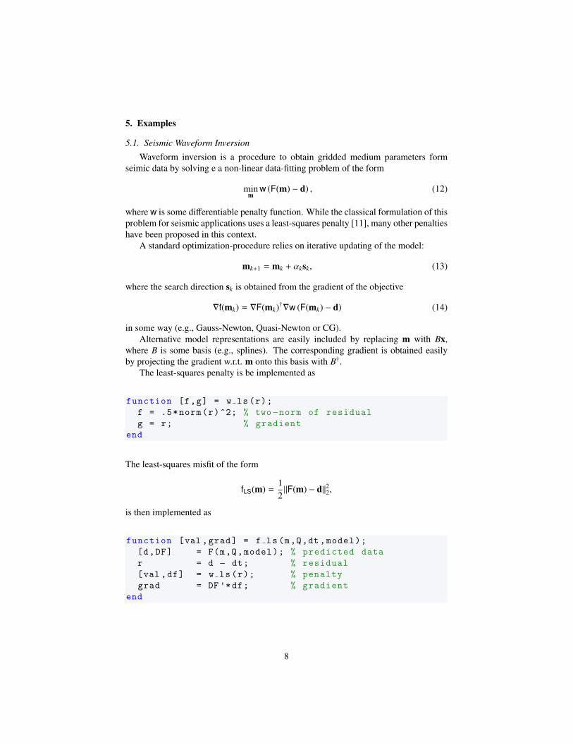
5.1. Seismic Waveform Inversion

Waveform inversion is a procedure to obtain gridded medium parameters formseimic data by solving e a non-linear data-fitting problem of the form

minm

w (F(m) − d) , (12)

where w is some differentiable penalty function. While the classical formulation of thisproblem for seismic applications uses a least-squares penalty [11], many other penaltieshave been proposed in this context.

A standard optimization-procedure relies on iterative updating of the model:

mk+1 = mk + αksk, (13)

where the search direction sk is obtained from the gradient of the objective

∇f(mk) = ∇F(mk)†∇w (F(mk) − d) (14)

in some way (e.g., Gauss-Newton, Quasi-Newton or CG).Alternative model representations are easily included by replacing m with Bx,

where B is some basis (e.g., splines). The corresponding gradient is obtained easilyby projecting the gradient w.r.t. m onto this basis with B†.

The least-squares penalty is be implemented as

function [f,g] = w ls (r);

f = .5∗norm(r)^2; % two−norm of residual

g = r; % gradient

end

The least-squares misfit of the form

fLS(m) =12||F(m) − d||22,

is then implemented as

function [val ,grad] = f ls (m,Q,dt,model);

[d,DF] = F(m,Q,model); % predicted data

r = d − dt; % residual

[val ,df] = w ls (r); % penalty

grad = DF '∗df; % gradient

end

8

This function can be passed on to any black-box optimization method that uses onlyfunction-values and gradients. A Gauss-Newton method can be easily implemented byhaving the function return the Gauss-Newton Hessian as SPOT operator.

To illustrate the approach we use the BG Compass velocity model depicted in figure5 (a). We generate data for this model for 71 sources and 281 receivers, all equi-spaced and located at the top of the model. For the inversion we use a multi-scalestrategy [12], inverting the data in consecutive frequency bands f1 = {2.5, 3, 3.5}, f2 =

{5.5, 6, 6.5}, f3 = {11.5, 12, 12.5}, f4 = {17.5, 18, 18.5}, each time using the end resultas initial guess for the next frequency band. The initial model for the first frequencyband is depicted in figure 5 (b). We use 10 L-BFGS iterations for each frequency band.The results are depicted in figure 6.

5.2. Reverse time migration

A seismic image can be obtained from reflection data via backpropagation

δm = ∇F†δd. (15)

This is referred to as reverse-time migration in the geophysical literature. The factthat this simple backprojection yields a useable image at all is due to the fact that theNormal operator ∇F†∇F acts as local scaling and filtering operation only [13]. Manyapproaches have been developed to estimate the inverse of this filter without explicitlyinverting the normal operator. Following [14] we estimate the image as

δm = Wx∇F†diag(wω)d, (16)

where Wx represents the spatial weighting and wω represents a frequency-weighting|ω|−1. Herrmann et al. [14] take Wx to be a diagonal weighting in the Curvelet domain.For the sake of this example, however, we use a simple spatial weighting that correctsfor the geometric spreading: Wx = diag(

√z).

The following code implements this procedure:

% reverse time migration for given data d and ...

background model m0

% get data and Jacobian

[d0,DF] = F(m0,Q,model);

% weighting with | \ omega |^ { −1 }

Wf = oppKron2Lo(opDiag (1./freq),opDirac(nsrc∗nrec));

% depth weighting

Wz = opKron(opDirac(n(2)),opDiag(sqrt(z)));

% reverse−time migration

dm = Wz∗DF '∗(Wf∗(d − d0));

9

Note the use of the parallel Kronecker product oppKron2Lo which works on arraysthat are distributed along the last dimension (frequency, in this case). To avoid artifactsdue to non-reflected events in the data, I subtract data for the background model. Iillustrate the algorithm on the Marmousi model, depicted in figure 7 (a), using 101sources, 201 receivers (equispaced at the top of the model) and frequencies between2.5 and 20 Hz with 0.5 Hz increments. The background model, depicted in figure 7 (b),is a smooth version of this model. The true perturbation (i.e., the difference betweenthe true and background model) is shown in figure 7 (c). The resulting image is shownin figure 7 (d).

5.3. Seismic tomography

Tomographic inversion relies on traveltime information to invert for the velocity.Traditionally, traveltimes are manually picked from the data and predicted traveltimesare computed using a geometric-optics approximating as is also used x-ray tomography.The last two decades there has been an increasing interest in generalizing this approachto finite-frequency regime where wave propagation is no longer accurately modeled viarays. One way to define the finite-frequency traveltime is to consider the correlation ofthe observed data with the data for some reference model, and pick the maximum[15]. The observed traveltime difference w.r.t. to the reference model for source i andreceiver j is then given by

δtobsi j = argmax

t

∑ω

(di j(ω)

)∗dobs

i j (ω)eıωt, (17)

where dobsi j (ω) is the observed data and di j(ω) is the modeled data for the reference

model (i.e., d = F(m0)). By correlating the data for the reference model with predicteddata for a model m we can compute the predicted traveltime difference δt(m) in asimilar manner. The goal then is to find a model m such that δt(m) ≈ δtobs. Forthe purpose of inversion the relation between the traveltime difference and the modelperturbation δm = m −m0 is usually linearized, yielding

δti j =

∑ω ıω

(di j(ω)

)∗δdi j(ω)∑

ω ω2|di j(ω)|2

, (18)

where δdi j(ω) is the linearized data for the model perturbation δm (i.e., δd = ∇F(m0)δm).We can write this relation as δt = Kδm, where the rows of K are the so-called sensitiv-ity kernels. For an in-depth overview and further references we refer to [16].

In case of constant reference velocity we can implement the (linearized) scatteringoperator using the Greens function:

δd(ω) = ω2Gr(ω)diag(δm)Gs(ω), (19)

where Gr denotes the Greens function from the receivers to the subsurface and Gs

denotes the Greens function from the subsurface to the sources.

function output = Ktomo(v0,input ,flag)

10

% get reference wavefield and scale factor

for k = 1: nfreq

d ref (:,:,k) = ... % reference data

scale = scale + omega(k)^2∗ abs( d ref (:,:,k));

end

% input

if flag > 0

output = zeros(nrec ,nsrc);

else

input = reshape(input ,[nrec ,nsrc])./scale;

output = zeros(nz∗nx ,1);end

for k = 1: nfreq % loop over frequencies

Gs = ... % source wavefield

Gr = ... % receiver wavefield

if flag > 0 % forward mode

d scat = omega(k)^2∗Gr∗diag(input)∗Gs;output = output + ...

1i∗omega(k)∗conj( d ref (:,:,k)).∗ d scat ;

else % adjoint mode

input k = −1i∗omega(k)∗ d ref (:,:,k).∗input;output = output + ...

omega(k)^2∗ diag(Gr '∗ input k ∗Gs ');end

end

% output

if flag > 0

output = vec(output./scale);

end

end

To illustrate the method, I use the velocity model depicted in figure 8 (a). The dataare modeled for frequencies 0.5 Hz to 20 Hz with 0.5 Hz increments and 21 sources and21 receivers which are equally distributed along vertical lines on the left and right sideof the model at x = 10 and x = 990 respectively. As outlined above, the traveltime dataare obtained by correlating this data with the data for the reference model (a constantvelocity of 2000 m/s in this case), and picking the maximum value for each source-receiver pair. The resulting traveltime data is shown in figure 8 (b). An example of

11

the corresponding waveform data for the true and reference model is shown in figures8 (c,d). The correlation panel and the picked traveltimes are shown in figure 8 (c).The scattering operator is implemented using the analytic expression for the Greensfunction discussed earlier. An example of the sensitivity kernel for one source andreceiver is shown in figure 9 (a). Smoothness is imposed on the solution by representingthe model on a coarser grid with cubic splines. For this example, the spline grid isdefined as Bx = {100, 300, 500, . . . , 900} and Bz = {100, 200, 300, . . . , 900}. For thethe spline evaluation I use opSpline1D with Dirichlet boundary conditions in the zdirection and Neumann boundary conditions in the x direction. Matlab’s lsqr is usedto solve the resulting linear system. The results after 10 iterations is shown in figure 9(b). The code to perform this experiment is given by

% spline grid

xs = [100:200:900];

zs = [100:100:900];

% spline operators

Bx = opSpline1D(xs ,x,[1 1]);

Bz = opSpline2D(zs ,z,[0 0]);

B = opKron(Bx,Bz);

% wrap function Ktomo in SPOT operator

K = opFunction(...

% call LSQR

dm = lsqr(K∗B,T,1e−6,10);

6. Conclusion and discussion

I present a flexible and scalable framework for prototyping algorithms for seismicimaging and inversion. The code can be useful for other applications, such as Medicalimaging [17].

Separate pieces of the code can be easily swapped out. For example, we can use adifferent wave-equation and leave the rest of the code unchanged. The use of operatoroverloading allows us to easily interface with existing optimization codes.

The object-oriented approach, of which this framework is an example, allows usto design complicated algorithms from relatively simple, easy to maintain, buildingblocks. Although the current implementation is done in Matlab, a similar frameworkcan be realized in lower level languages using existing libraries such the Rice VectorLibrary.

Future work will be aimed at further abstraction of data-structures. Matlab alreadyallows us to work with distributed arrays with relative ease by taking care of commu-nication automatically. In a similar fashion, we can use the memmap functionality to

12

acces data that is stored on disk as if it was a Matlab array. Such an approach wouldallow us to scale the same algorithms to very large data-sets, for example by adoptingGoogle’s MapReduce model [18].

AcknowledgmentsI thank everybody at the Seismic Laboratory for Imaging and Modeling (SLIM)

at UBC for their feedback and help with developing this software. The BG Compassvelocity model was made available by the BG Group. This work was in part finan-cially supported by the Natural Sciences and Engineering Research Council of CanadaDiscovery Grant (22R81254) and the Collaborative Research and Development GrantDNOISE II (375142-08). This research was carried out as part of the SINBAD IIproject with support from the following organizations: BG Group, BP, Chevron, Cono-coPhillips, Petrobras, Total SA, and WesternGeco.

13

[1] J. Claerbout, S. Fomel, IMAGE ESTIMATION BY EXAMPLE: GeophysicalSoundings Image Construction, 2012.URL http://sepwww.stanford.edu/sep/prof/gee8.08.pdf

[2] W. W. Symes, D. Sun, M. Enriquez, From modelling to inversion: designing awelladapted simulator, Geophysical Prospecting 59 (5) (2011) 814–833. doi:10.1111/j.1365-2478.2011.00977.x.

[3] S. Balay, W. D. Gropp, L. C. McInnes, B. F. Smith, Efficient management ofparallelism in object oriented numerical software libraries, in: E. Arge, A. M.Bruaset, H. P. Langtangen (Eds.), Modern Software Tools in Scientific Comput-ing, Birkhauser Press, 1997, pp. 163–202.URL http://dl.acm.org/citation.cfm?id=266469.266486

[4] M. A. Heroux, R. A. Bartlett, V. E. Howle, R. J. Hoekstra, J. J. Hu, T. G. Kolda,R. B. Lehoucq, K. R. Long, R. P. Pawlowski, E. T. Phipps, A. G. Salinger, H. K.Thornquist, R. S. Tuminaro, J. M. Willenbring, A. Williams, K. S. Stanley, Anoverview of the trilinos project, ACM Trans. Math. Softw. 31 (3) (2005) 397–423.doi:10.1145/1089014.1089021.

[5] A. D. Padula, S. D. Scott, W. W. Symes, A software framework for abstractexpression of coordinate-free linear algebra and optimization algorithms, ACMTransactions on Mathematical Software 36 (2) (2009) 1–36. doi:10.1145/1499096.1499097.

[6] E. van den Berg, M. P. Friedlander, Spot A Linear-Operator Toolbox (2009).URL http://www.cs.ubc.ca/labs/scl/spot/

[7] B. N. Kuvshinov, W. A. Mulder, The exact solution of the time-harmonic waveequation for a linear velocity profile, Geophysical Journal International 167 (2)(2006) 659–662. doi:10.1111/j.1365-246X.2006.03194.x.

[8] H. Modzelewski, T. Lai, S. Jalali, pSPOT, a parallel extension of SPOT (2010).URL https://github.com/slimgroup/pSPOT

[9] S. Pacteau, pSPOT, a parallel linear operator toolbox, Tech. rep. (2010).URL http://slim.eos.ubc.ca/Publications/Public/TechReports/

Internship_report_last.pdf

[10] C.-H. Jo, An optimal 9-point, finite-difference, frequency-space, 2-D scalar waveextrapolator, Geophysics 61 (2) (1996) 529. doi:10.1190/1.1443979.

[11] A. Tarantola, A. Valette, Generalized nonlinear inverse problems solved using theleast squares criterion, Reviews of Geophysics and Space Physics 20 (2) (1982)129–232.

[12] L. Sirgue, R. G. Pratt, Efficient waveform inversion and imaging: a strategy forselecting temporal frequencies, Geophysics 69 (1) (2004) 231–248. doi:10.1190/1.1649391.

14

[13] W. W. Symes, Approximate linearized inversion by optimal scaling of prestackdepth migration, Geophysics 73 (2) (2008) R23–R35. doi:10.1190/1.

2836323.

[14] F. J. Herrmann, P. P. Moghaddam, C. C. Stolk, Sparsity- and continuity-promotingseismic image recovery with curvelet frames, Applied and Computational Har-monic Analysis 24 (2) (2008) 150–173. doi:10.1016/j.acha.2007.06.007.

[15] Y. Luo, Wave-equation traveltime inversion, Geophysics 56 (5) (1991) 645. doi:10.1190/1.1443081.

[16] A. Fichtner, Full Seismic Waveform Modelling and Inversion, Springer Verlag,2010.URL http://www.springer.com/earth+sciences+and+geography/

geophysics/book/978-3-642-15806-3

[17] F. Natterer, F. Wubbeling, Mathematical Methods in Image Reconstruction,Mathematical Modeling and Computation, SIAM, 2001. doi:10.1137/1.

9780898718324.

[18] J. Dean, S. Ghemawat, Mapreduce: simplified data processing on large clusters,in: Proceedings of the 6th conference on Symposium on Opearting Systems De-sign & Implementation - Volume 6, OSDI’04, USENIX Association, Berkeley,CA, USA, 2004, pp. 10–10.URL http://dl.acm.org/citation.cfm?id=1251254.1251264

15

linear quadratic cubic0 0.000000e+00 0.000000e+00 0.000000e+001 0.000000e+00 5.551115e-17 5.551115e-172 1.000000e-02 0.000000e+00 0.000000e+003 1.500000e-02 3.000000e-03 0.000000e+004 1.510000e-02 5.100000e-03 9.000000e-045 1.275000e-02 5.550000e-03 2.250000e-03

Table 1: Accuracy of the discretized delta function for l = 0, 1, . . . , 5 using linear, quadratic and cubicinterpolation.

<〈Ax, y〉 <〈x, A†y〉 error2.453000e+07 2.453000e+07 2.220400e-141.762400e+08 1.762400e+08 3.552700e-151.896000e+08 1.896000e+08 1.421100e-14-4.902800e+07 -4.902800e+07 7.194200e-141.295700e+08 1.295700e+08 3.197400e-14-4.529400e+08 -4.529400e+08 3.197400e-14-1.711600e+08 -1.711600e+08 3.206300e-13-3.416800e+08 -3.416800e+08 0.000000e+00-8.159100e+08 -8.159100e+08 1.421100e-143.125000e+07 3.125000e+07 7.993600e-15

Table 2: Dot-test of Jacobian on random test vectors.

# of procs time [s] efficiency1.00 2459.00 1.002.00 1224.00 1.004.00 615.00 1.008.00 313.00 0.98

16.00 188.00 0.82

Table 3: We compute data for a 1200x404 model for 64 frequencies and 10 sources using different numbersof CPUs. The times are averages over 5 runs.

16

Figure 1: Illustration of grids used for modeling. The physical grid (white) is extended on all sides (grey) todefine the computational grid. Examples of the source and receiver grids are also shown.

0 0.2 0.4 0.6 0.8 1−0.2

0

0.2

0.4

0.6

0.8

xC

linear

quadratic

cubic

Figure 2: Discretization of a delta function δ(x − 12 ) using linear, quadratic and cubic interpolation.

17

101

100

101

102

103

h

err

or

0 200 400 600 800 1000−4

−3

−2

−1

0

1

x [m]

z [m

]

Re(numerical)

Re(analytic)

Im(numerical)

Im(analytic)

(a) (b)

x [km]

z [km

]

0 1 2 3 4 5

0

0.5

1

x [km]

z [km

]

0 1 2 3 4 5

0

0.5

1

(c) (d)

Figure 3: Accuracy of the modeling operator. (a) error between analytic and numerical solution for constantvelocity v0 = 2000 m/s and a frequency of 10 Hz. on a domain of 1000 m× 1000 m with a point sourcein the center. (b) Wavefields at z = 500m. (c-d) Analytic and numerical solution for linear velocity profile2000 + 0.7z and a frequency of 10 Hz.

10−6

10−4

10−2

100

10−10

10−5

100

105

h

err

or

Figure 4: bla

x [km]

z [km

]

0 2 4 6

0

1

2

x [km]

z [km

]

0 2 4 6

0

1

2

(a) (b)

Figure 5: (a) BG Compass velocity model and (b) initial model for FWI example.

18

x [km]

z [km

]

0 2 4 6

0

1

2

x [km]

z [km

]

0 2 4 6

0

1

2

(a) (b)

x [km]

z [km

]

0 2 4 6

0

1

2

x [km]

z [km

]

0 2 4 6

0

1

2

(c) (d)

Figure 6: Result of the inversion of subsequent frequency bands: (a) 2.5-3.5 Hz, (b) 5.5-6.5 Hz, (c) 11.5-12.5Hz and (d) 17.5-18.8 Hz, each after 10 L-BFGS iterations using the previous result as starting model.

x [m]

z [m

]

0 2000 4000

0

1000

2000

3000 2000

3000

4000

x [m]

z [m

]

0 2000 4000

0

1000

2000

3000 2000

3000

4000

(a) (b)

x [m]

z [m

]

0 2000 4000

0

1000

2000

3000

x [m]

z [m

]

0 2000 4000

0

1000

2000

3000

(a) (b)

Figure 7: (a) Marmousi velocity model (m/s). (b) Background model used for imaging (m/s). (c) trueperturbation. (d) image.

19

x [m]

z [m

]

0 500 1000

0

200

400

600

800

1000 1800

1900

2000

2100

2200

2300

2400

2500

zr [m]

zs [

m]

0 500 1000

0

200

400

600

800

1000

−0.01

0

0.01

0.02

0.03

(a) (b)

zr [

m]

t [s]0 0.5 1

0

200

400

600

800

1000

zr [

m]

t [s]0 0.5 1

0

200

400

600

800

1000

zr [

m]

∆ t [s]−0.2 0 0.2

0

200

400

600

800

1000

(c) (d) (e)

Figure 8: The velocity model (m/s) used in tomographic example is shown in (a), the corresponding trav-eltime data (s) for each source-receive pair is shown in (b). The waveform data for a source located atx = 10, z = 500 is depicted in (b); (c) shows the data for the initial homogeneous velocity (2000 m/s) and (d)shows the correlation of these two and the picked traveltimes.

x [m]

z [m

]

0 500 1000

0

200

400

600

800

1000

x [m]

z [m

]

0 500 1000

0

200

400

600

800

1000

(a) (b)

Figure 9: (a) sensitivity kernel for one source-receiver pair. (b) reconstruction after 20 LSQR iterations onthe same colorscale as figure 8 (a).

20

Appendix A. Matlab Package

The Matlab code can be downloaded from https://www.slim.eos.ubc.ca/releases. It has been tested with Matlab 2011b. The Parallel Computing Toolboxis needed to take advantage of the parallelism, though the code will run in serial modelwithout the toolbox as well.

Below is a short description of the contents of the package.

tools/utilities/

• SPOT-SLIM – SPOT toolbox

• pSPOT – pSPOT toolbox

tools/algorithms/2DFreqModeling/

• F – Modelling operator

• DF – Jacobian of F

• oppDF – pSPOT constructor of Jacobian, uses DF

• G – Modelling operator for velocity of the form v(z) = v0 + αz

• legendreQ – evaluates the Legendre Q function Qν(z)

• Helm2D – discretized Helmholtz operator

tools/operators/misc/

• opLinterp1D – 1D cubic Lagrange interpolation

• opLinterp2D – 2D linear Lagrange interpolation

• opSpline1D – 1D Cubic Spline evaluation

• opSpline2D – 2D Cubic Spline evaluation

• opExtension – 1D padding

• opDFTR – Fourier transform for real signals; returns only positive frequencies.

tools/functions/misc/

• vec, invvec – vectorize (distributed) array and reshape (distributed) – vectorback to (distributed) n-dimensional array.

• odn2grid, grid2odn – convert offset-increment-size vectors to grid vectorsand vice-versa.

• odnread, odnwrite – read/write for gridded data.

tools/solvers/QuasiNewton/

• lbfgs – L-BFGS method with weak Wolfe linesearch

21

applications/SoftwareDemos/2DSMII

• mbin/f ls – Least-squares misfit and gradient

• mbin/w ls – compute two-norm of vector and its gradient.

• mbin/Ktomo – Scattering operator for traveltime tomography example

• scripts – scripts to produce examples

• doc – documentation in html format

22