A Parallel Processing Algorithm for Remote Sensing Classification

J. Anthony Gualtieri Code 606.3 and Global Sciences and Technology

NASA/GSFC Greenbelt, Maryland 20771 gualt @backsem .gsfc .nasa. gov

I Introduction

A current thread in parallel computation is the use of cluster computers created by networking a few to thousands of commodity general-purpose workstation-level commuters using the Linux operating system. For example on the Medusa cluster at NASA/GSFC, this provides for super computing performance, 130 Gflops (Linpack Benchmark) at moderate cost, $370K. However, to be useful for scientific computing in the area of Earth science, issues of ease of programming, access to existing scientific libraries, and portability of existing code need to be considered. In this paper, I address these issues in the context of tools for rendering earth science remote sensing data into useful products. In particular, I focus on a problem that can be decomposed into a set of independent tasks, which on a serial computer would be performed sequentially, but with a cluster computer can be performed in parallel, giving an obvious speedup. To make the ideas concrete, I consider the problem of classifying hyperspectral imagery where some ground truth is available to train the classifier. In particular I will use the Support Vector Machine (SVM) approach as applied to hyperspectral imagery [16].

The approach will be to introduce notions about parallel computation and then to restrict the development to the SVM problem. Pseudocode (an outline of the computation) will be described and then details specific to the implementation will be given. Then timing results will be reported to show what speedups are possible using parallel computation. The paper will close with a discussion of the results.

2 Supervised Classification of Hyperspectral Data

I will address the problem of supervised classification of hyperspectral images working only in the spectral domain. Because the data is high dimensional, in that there are hundreds of channels of spectral information per pixel comprising a spectra and represented as a vector of values, algorithms that use all of the channels can be computationally expensive. The traditional approach to handling this is to perform a pre-processing dimension reduction step, but this removes valuable information. Here we will use an algorithm that uses all the channels.

For supervised classification, the problem separates into a training phase and a testing phase. For the training phase we are given exemplars with class labels, in this case the spectra associated to the ground truth pixels in the scene. These are used to train the classifier. In the testing phase the trained classifier is then applied to pixels not yet classified and not used in the training phase.

lThe term "machine" in Support Vector Machine is only a name and does not imply a hardware device.

1

https://ntrs.nasa.gov/search.jsp?R=20050180255 2018-08-23T04:01:52+00:00Z

2.1 Simplifying Classification with Many Classes

L

O(K2m2) O(K3m2) J

K ( K - 1)/2*0(m2) K*O(((K - l)? + ?)2)

2.1.1 Training

Given we have an algorithm to classify a pair of classes, how do we build classification algorithms that can handle multiple classes? Let K be the number of classes, where K M 10.. ,20 and more, and where each class contains varying numbers of training vectors (spectra in the case of hyperspectral imagery). A successful strategy to cope with large numbers of classes is to decompose the problem into a number of simpler classification problems that each deal with only pairs of classes. One such method is to train over all possible pairs of classes, K ( K - 1)/2, in number, and then use some voting scheme in the testing phase of the classification. Call this the K choose 2 method. An alternative approach is to train K pair classifiers, each of the form 1 versus K - 1 and then in the testing phase compare results from the K classifiers to render a classification. Call this the 1 vs. K - 1 method. The second method involves a heavy burden on training the K such classifiers, one for each class, because there will be many training spectra from the K - 1 classes that are lumped together for training. The SVM training algorithm has computational complexity O(m2), where m is the number of training vectors in the pair of classes. Computational complexity here means how the time to complete the computation on a single processor scales in terms of the number of units of data, m, to be processed - in this case the number of training spectra. Thus, if time to completion is given by t = Am2 + Brn + C, where t is time to completion, and A, B , C are constants, then t N O(m2). To obtain an estimate of the complexities of the two methods, assume each training class is the same size, 3. Then the time complexity for the two approaches is given in Table 1. In the left column is the K choose 2 approach and in the right column is the 1 vs. K - 1 approach. The second row indicates where these results come from.

Table 1: Time complexity on a single processor for performing SVM training for a classifier of K classes each containing m / 2 exemplars.

K choose 2 I ~ V S . K - 1 1

There is a time complexity advantage to using the K choose 2 method. We adopt this approach in the what follows. In addition, there is some evidence that the K choose 2 method is more accurate than the 1 vs. K - 1 method [17]. For the K choose 2 method, simple parallelism can be readily obtained by putting each pair-training computation on a different processor on the cluster machine. If there are more pairs than processors, then they are stacked onto processors and solved sequentially. Note we will not parallelize the basic pair-training algorithm as this would require having detailed knowledge of the SVM training algorithm optimization method, though see [28], for results from such an approach for training a pair classifier with very large numbers of training vectors.

2.1.2 Testing

Once we have trained the K ( K - 1)/2 pair classifiers, we obtain the classification in the testing phase by applying all the pair classifiers to each spectra (one per pixel) to be classified, and for each pair noting which of the two classes is found for that pixel. Then all K ( K - 1)/2 results per pixel (think of votes) are placed into one of K bins and the bin with the largest number of votes is declared the class for that pixel. For ties in the number of votes, either a random selection is made or some refinement using a numerical measure from the pair classifier is used. Thus, if we define Vr E [I,. . . , K ] as the classification label for the pixel at position r, then the winning class label at pixel r is given by

I

where for pair classifier i, j ,

i if class i wins over class j j if class j wins over class i 9

vr(i’j) = { and

1 i f m = n 0 i f m f n &n,n =

is the Kronecker delta function.

Here parallelism can be used in several ways. We can use a single processor testing code for all K(K-1)/2 pairs, and segment the imagery into tiles that cover the whole scene, and process the tiles each on a different processor. Or we may use a single processor code that implements the testing phase for each of the K(K-1)/2 pair classifiers applied to the whole image on a single processor, and follow this with a voting scheme to obtain the final classification. The voting scheme part could be run on a single processor as it is likely to be very fast, or if need be, applied on different processors in a tiling of the image.

2.2 The Support Vector Machine Algorithm

The basic algorithm used in this paper to perform supervised classification of hyperspectral remote sensing data is the SVM coupled with the Kernel Method [25]. Previous work using the SVM algorithm together with the Kernel Method derives from the machine-learning community, with methods pioneered by Vapnick, and extended by Boser, Guyon, and Vapnick [2], and Cortes and Vapnick [6]. In particular the SVM approach yields good performance on high-dimensional data such as hyperspectral imagery, and does not suffer from the curse of dimensionality [l], which limits the effectiveness of conventional classifiers due to the Hughes effect [18]. This because the SVM classifier depends on only a small subset of the training vectors, called the support vectors, which define the classifier as used in the testing phase.

Application of SVM to hyperspectral data was first demonstrated by Gualtieri and co-workers in [16] [15] [14]. I direct the reader to those references for details of the SVM formulation and application to several hyperspectral data sets, including Indian Pines 1992 of image size 145 x 145 with 200 bands and 16 classes [22], and Salinas 1998 with image size 512 x 215 with 224 and 16 classes [21]. In the reported work above, all implementations were performed on a single workstation class processor and used T. Joachim’s open source SVMlight package [19] [20]. The most computationally expensive task within the SVM training requires quadratic optimization, for which A. Smolla’s open source PRLOQO was used [26]. More recent work [29] [23] 141 [3]. has provided further validation of SVM’s utility for hyperspectral classification.

3 Parallel Implementation for Supervised Learning by Porting Serial Code

We take as given a serial code for performing SVM training and testing for classification of hyperspectral data. Here we introduce more of the details of the parallel computation and demonstrate how the serial code can be adapted to parallel computation.

2A 145 x 145 pixel and 220 band subset in BIL format of radiance data that has been scaled and offset to digital numbers, DN, from radiance, rad in units W/(cm2 * n m * S T ) according to DN = 500 * rad + 1000 as 2bit signed integers. It is available at ftp://ftp.ecn.purdue.edu/biehl/MultiSpec/92AV3C. Ground truth is also available at ftp://ftp.ecn.purdue. edu/pub/biehl/PC-Mu$tiSpec/ThyFiles .zip. The full data set is called Indian Pines 1 f920612tOlp02~02 as listed in the AVIFUS JPL repository (http: //aviris. jpl.nasa.gov/ql/list92. html). The flight line is LatStart: 40:36:39 LongStart: -8702:21 LatEnd: 40:10:17 LongEnd: -87:02:21 Start-Time:19:42:43GMT End-Time:19:46:2GMT. See also http: //dynamo. ecn.purdue.edu/-biehl/MultiSpec/aviris_documentation.html

3AVIlUS Hyperpsectral Radiance Data from f981009tOlr-07. The full flight line is 961 samples by 3479 lines consisting of 224 bands of BIP calibrated radiance data that is scaled to lie in [O,lOOOO] as 2bit signed integers. We have studied part of scene 3. The full flight line is called f981006t01p01-r07 as listed in the AVIFUS JPC repository. The flight line is [LatStart: +36-15.0 LongStart: -121-13.5 LatEnd: +36-21.0 LongXnd: -121-13.5 Start-Time: 1945:30GMT End-Time: 1950:15GMT.

3

3.1

For parallel programming, currently the most popular model is Multiple Instruction Multiple Data (MIMD) . Here each of the processors can perform different instructions on different data, and there is no synchroniza- tion of the processor clocks. Because of the lack of explicit synchronization, any interprocessor communication must be explicitly initialized and and then tested for completion at the sending and the receiving processors, if subsequent processing is to remain synchronized. This overhead of testing for completion is assumed to be the responsibility of the programmer, and is part of what makes this programming model difficult to use.

Such MIMD machines may or may not have a shared memory system among all the processors, but the most typical use a collection of nodes each consisting of a symmetric multiprocessor (SMP) with a shared memory and shared disk. Typically each SMP node may comprise two to four single processors. Here shared memory is only at the nodes. In the sequel we will take the basic unit of computation as the processor. The differences in communication within a node and between nodes will not be considered, which is reasonable given the particular problems we solve. This particular hardware configuration is called a Beowulf cluster and can consist of a few to hundreds of nodes [27].

Programming Model, Hardware, Message-Passing Interface

The software used here to coordinate the processors is the Message Passing Interface (MPI) [lo] [8] [13]. MPI extends the C and C++ languages (or Fortran ) with a set of subroutines that implement communication and data movement among unsynchronized processors, and provides for methods to test for synchronization. With careful layout of data and communications, the multiple processors can divide up a computation efficiently, although there is a heavy load on the programmer to craft the code. The actual code used in any particular parallel problem is heavily problem dependent.

3.2 Pleasingly Parallel Problems

If we can decompose the serial code into a series of tasks with minimal communication between the tasks, namely at the beginning and ending of the tasks, then the porting of the serial code fits under the rubric of

As an example, consider problems involving imagery where the spatial coordinates do not enter explicitly into the computation. A decomposition can result from dividing the image into tiles on which the same computation is to be performed. A very simple example would be normalizing an image by dividing by a given constant value. In a serial machine code, a loop over all N pixels is run, and each pixel is normalized one after the other, taking O ( N ) time. In a parallel setting, if we had as many processors as pixels, then each processor would perform one division operation taking O(1) time. For comparison, a less trivial task would be to find a normalization factor by adding values from each pixel and dividing by the number of pixels. On a parallel machine, explicit communication between nodes would be required as part of the task. In fact, this can be accomplished in O(1ogzN). See Appendix A.

/pleasingly parallel.

The SVM training and testing problem we address here can be thought of as having a simple decompo- sition into independent parts that can be processed, with communication occurring only at the start and finish of each task.

3.3 Organizing the Problem

Let us now consider how to organize a cluster computer for a pleasingly parallel problem with np number of processors and nt number of independent tasks. Call the set of tasks the task list. We wish to find an approach that keeps all the processors busy as much of the time as possible. If the size of the task list is nt 5 np, then put one task on each processor and wait until the last task completes.

If nt > np, a naive solution would be to first put an equal number of tasks, Lnt/np],

1.1 is the floor function, defined as the nearest integer to z that is smaller than or equal to x.

on each processor

4This is also referred to as embarrassingly parallel in that, in principle the decomposition of the problem is trivial.

4

and let them run sequentially on each processor until complete. If there are remaining tasks, nrem = nt - Lnt/npJ # 0, then put these last tasks on any of n,,, processors. However, this will be efficient only if all tasks take the same amount of time. This solution is like the queuing problem in a bank where a large number of people enter at one time and each go to a teller in a separate queue. If no more people enter and once in a line you cannot shift, then roughly the lines start out at the same length. However, as transaction duration for each person varies, some people will have longer waits than others while evefitually some tellers will have no customers. For SVM, the training times will be different because of different numbers of training vectors in the classes to be trained on.

At this point, note that it has not been said where the original complete task list lives, or how the task list is divided up and communicated among the processors. This is taken care of by designating a particular processor of the cluster as the boss processor, whose job is to manage the apportioning of the task list and the communication of tasks to the remaining processors, which are called the worker processors. Then with the boss processor able to monitor the status of each worker processor, the boss processor can, first using a list of tasks waiting to be done, send one each to all the worker processors and thereafter wait for workers to be done and then send the next task in the list to that worker processor. In this way, all the worker processors are always busy. We have implemented this approach in prototype program called boss-workers and subsequently mapped the learning phase and the testing phase of the supervised classification onto it. However, there still remain issues concerning the sending and receiving of communications from the boss to the worker, and from the worker to the boss. We address this below.

3.4 Aspects of Communication in MPI

Here we give an overview of how to handle the asynchronous communication between processors in the MPI language for this particular application. Communications consists of two parts, sending and receiving. To describe this process we use a metaphor based on the postal system and described in Table 2. Here buffer is

Table 2: Postal system analogy to MPI send and receive statements.

Postal System MPI sender writes letter sender posts letter and waits for notice of receipt recipient waits for mail t o be received recipient reads letter

sender loads buffer sender executes MPISend on buffer receiver executes MPIReceive on buffer receiver unloads buffer

a piece of memory available to the sending and receiving processor. Note that MPISend and MPIReceive do not “simply post the letter” or check for “receipt of a letter”, and then continue to do other things. These MPI statements are called blocking send and receives, and they cause the processor to wait for completion before continuing to the next statement in the code. This may have a problematic side effect as illustrated in Table 3, showing deadlocking involving executing MPISend and MPIReceive on processors i and j. The

Table 3: Deadlocking in MPI.

processor i processor j MPI-Send(j) MPI-Send(i) MPI-Recv(j) MPIRecv(i)

problem is that it is possible, depending on buffer size, for neither MPISend(i) or MPISend(j) to complete because each MPISend awaits the execution of the MPIRecv on the other processor, which cannot be reached.

I To handle this problem and to make MPI code safe, meaning here that deadlocking cannot occur, MPI provides a second kind of Send and Recv called non-blocking designated MPIlSend and MPIJRecv. These statements post the send and receive messages, but do not wait for completion. Now to know if the messages are completed, another class of MPI statements called MPI-Wait is needed.

,

I 3.5 Boss-workers algorithm in MPI

Now we can can give an abstract version of the bosssorkers algorithm written in pseudocode. In pro- gramming in MPI the approach is to write a single code that will be running simultaneously on the boss and the worker processors. Thus, we can have sections of identical code running on all the processors, albeit not synchronized, or we can can have sections that are specific to one or more processors. The overall code makes this distinction by using a function in MPI that returns the number of the processor it is running on. By testing on this number in an i f or case statement, we can designate in the single MPI code, sections that will run only on designated processors. In the boss-workers code, one processor, numbered 0, is the boss, and 1 . . . nwo,.ke,. are the workers. Communication issues here only involve the boss communicating with a worker. No worker-to-worker communication occurs.

We present below a simplified code for the boss-workers algorithm. The framework for this code is

book and on the web site of Peter Pacheco [24], with particular applicaton to matrix vector multiplication. However, for the classification problem, the worker tasks require different computational effort, and also

command MPI-wait some, [12]. Beside the communications, the computational parts are:

I described for the case of each task taking the same computational effort (same time to execute) in the

require a generalization. This has been provided by William Gropp in the example of the use of the MPI I

I make-taskl i s t , where the boss generates the tasks.

bossnmke-task, where the boss takes a particular task and creates data for a worker.

workersork takes the input data sent by the boss, and the worker creates an output that is returned to I the boss.

consume, where the boss takes the output from the worker and completes processing on that output.

In application to the training phase the worker-work would be replaced by a module that performs SVM supervised learning, which for training takes as input the pair of two sets of exemplar or training vectors and outputs a file describing the appropriate classifier in terms of the support vectors it finds. For the testing phase, the input is the set of classifiers found in the training phase, and the hyperspectral cube of unclassified data. The output is the classified image. In the following pseudocode, scalar variable declarations are not explicitly included while arrays a , b with n, rn elements, respectively, are explicitly declared with a l l o c a t e ( aE0:n-111, b[O:m-I] , . . .).

6The problem of safety and a related concept fairness can be resolved in a variety of ways. See [ll].

6

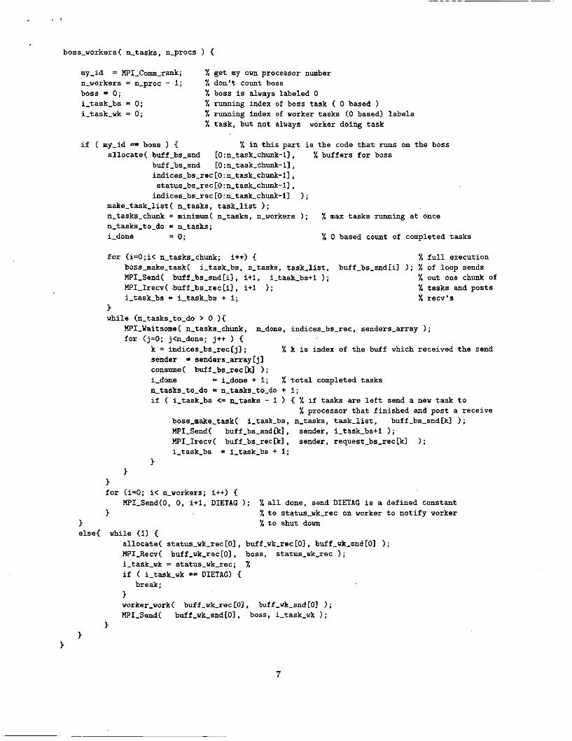
my-id = MPI-Comm-rank; % get my own processor number n-workers = n-proc - 1; boss = 0; i-task-bs = 0; i-task-wk = 0 ;

% don't count boss % boss is always labeled 0 % running index of boss task ( 0 based ) % running index of worker tasks (0 based) labels % task, but not always worker doing task

if ( my-id == boss ) { 1 in this part is the code that runs on the boss allocate( buff-bs-snd [O:n-task-chunk-lI, % buffers for boss

buff -bs-snd [O:n-task-chunk-ll, indices-bs-rec [O :n-task-chunk-l] , status-bs-rec [O :n-task-chunk-ll, indices-bs-rec [O:n-task-chunk-ll ;

make-task-list( n-tasks, task-list 1; n-tasks-chunk = minimum( n-tasks, n-workers ); n-tasks-to-do = n-tasks; i-done = 0; 1 0 based count of completed tasks

% max tasks running at once

for (i=O;i< n-tasks-chunk; i++) { % full execution boss-make-task( i-task-bs, n-tasks, task-list, buff-bs-snd[i] ; % of loop sends MPI-Send( buff-bs-snd[il, i+l, i-task-bs+l ; % out one chunk of MPI-Irecv( -buff -bs-rec [i] , i+l ; i-task-bs = i-task-bs + 1;

3 while (n-tasks-to-do > 0 ){

MPI-Waitsome( n-tasks-chunk, n-done, for (j=O; j<n-done; j++ 1 €

k = indices-bs,rec[j] ; % sender = senders-array [jl consume ( buff -bs-rec [kl ; i-done = i-done + I; % n-tasks-to-do = n-tasks-to-do + if ( i-task-bs <= n-tasks - 1

% tasks and posts % recv's

indices-bs-rec, senders-array ) ;

k is index of the buff which received the send

total completed tasks 1; { % if tasks are left send a new task to

% processor that finished and post a receive boss-make,task( i-task-bs, n-tasks , task-list , buff -bs-snd Ckl ; MpI-Send( b~ff-bs-snd[k], sender, i-task-bs+i ; MPI-Irecv( buff-bs-rec [kl , sender, request-bs-rec [kl ; i-task-bs = i-task-bs + I;

3 3

3 for (i=O; i< n-workers; i++) {

3 MPI-Send(O, 0, i+i, DIETAG ) ; % all done, send DIE'I" 1s a defined constant

1 to status-wk-rec on worker to notify worker 3 % to shut down else€ while (1) C

allocate( status-wk-rec [OI , buff-wk-rec [Ol, buff-Wk-snd[O] ; WI-Recv( buff-wk-rec[O]. boss, status-wk-rec ; i-task-wk = status-wk-rec; % if ( i-task-wk == DIETAG) {

3 worker-work( buff-wk-rec LO1 , buff-wk-snd Lo1 ) ; MPI-Send( buff-wk-snd[Ol, boss, i-task-wk ;

break;

3 3

3

4 Data Input and Output

A secondary issue is how data is to be passed to and from boss and workers. We can either have the boss read all the data and then explicitly pass the data to the workers at the time it is needed or we can make all the data available to the workers who then read the parts they need, based on names of data passed to them by the boss. Because the data set can be large, there are questions of how to best distribute the data to optimize overall computational time.

We elected to have all the input and output be processed by the workers, and have only labels describing the files to be input and output, passed by the boss to the workers. This finesses the passing of large data files between the boss and the workers, and places that burden on the file system of the cluster. For the benchmark computations of SVM training and testing, each node has its own copy of all required input files and writes only to its local disk.

It is possible to have all files shared by workers and boss by using Network File System (NFS), where the operating system passes copies of the needed file to the nodes as they need them. This effectively shares the same file system on all processors, and preliminary results for the SVM problem show similar performance. Note that the total size of the input data and output data in the training phase is 1.6 MB and 6.8 MB, respectively, and for the testing phase 23.6 MB and 2.5 MB, respectively. Given input/output (IO) speeds on the hardware used here, the time for IO of the data used here is small compared to processing times. However, for larger problems, the IO time costs may become significant, and different approaches may be needed for higher performance.

4.1 Details of the MPI Subroutines Used

The explanation of the MPI functions and a definition used in the pseudo code are:

MPISend( buff-bs-snd[i], i + l , i-task-bs+l ) This posts the data from the boss b u f f b s s n d [ i l . into the communication channel to processor i+i with message tag i - t a s k h s + l . Only when the buffer is received and emptied does it complete (blocking send).

MPI-Irecv( buf f -bsrec [ i ] , i+l ) This accepts the data into buff b s i e c [i] on the boss processor from the worker processor i+i and continues without waiting for completion (nonblocking receive).

MPI-Waitsome ( n-tasks-chunk, ndone , i n d i c e s b s i e c , sendersarray ) Waits for multiple com- munications to complete on the boss from n-tasks-chunk different workers. The quantity i n d i c e s h s i e c is an array of size n-tasks-chunk that contains the index identifying the receiving buffers among all the buffers b u f f - b s i e c [ ] corresponding to the members of the array sendersArray of size n-tasks-chunk, which contains the identities of the n-tasks-chunk senders.

MPI-Recv( buff -wkxec [O] , boss , s tatus-wkiec ) Blocking receive that accepts the data into the buffer buff - b s i e c [O] from the boss processor with resulting status written to the structure s tatus-wkiec .

DIETAG is a defined constant to signify work is completed.

In this implementation the buffers passed between boss and workers, buff b s s n d , buff b s i e c , buff -wksnd, and buff -wkiec, are very small structures containing labels describing files to be read by the workers, and timing information to be returned.

4.2 Implementation Details

In this code development for SVM, we opted to use a library of open source routines in C called LIBSVM, written by Chih-Chung Chang and Chih-Jen Lin [5]. In addition to a series of routines for input and output,

8

they have created a library of core subroutines and a set of data structures that we use in our parallel code. To handle hyperspectral data we have written our own IO routines as well as routines to convert from a hyperspectral cube to the data structure they use. These routines are then embedded into the boss-workers code.

In vanilla MPI only the single data type, vector, can be defined for the buffers that pass dztz to ar,d from the boss to the workers, however, it is extremely useful to be able to pass structures or other more complex data types in the buffers. One can use various MPI routines to do this, but a utility called AutoMap [7] automates this and is used in this implementation.

5 Timing and Speedup

To examine the performance of the parallelization of SVM code as implemented in the boss-workers al- gorithm, first we demonstrate the scaling of the speedup (ratio of single code execution time over parallel code execution time) for the b o s s s o r k e r s code on a very simple task. Here the work done on each worker processor is to make it sleep for a fixed length of time. Then as a benchmark of a real problem, we apply training and testing of the SVM to the well-studied hyperspectral data set, Indian Pines 1992 [22], of size [nl, ns, nb] = [145,145,200] with K = 16 classes. In what follows, all times reported are wall clock time, overall elapsed time, rather than actual computation time as performed by the processor. The times reported are based on the nodes in use having only one user. It is possible to have time sharing of parallel jobs, but this is not the case here.

5.1 Simple Validation

Let the work done on each worker processor be to sleep for a fixed length of time, say 5 s. We expect that if the number of processors matches the number of tasks, then total computing time will remain the same independent of the number of tasks. Table 4 shows the total time taken (wall-clock) assuming no other jobs running. Except for the jump of 1 s for np = 1 + 100, the results are consistent with the notions above. The slight increase in time is presumably due to the boss performing the overhead of managing the workers.

Table 4: Time to completion (s) and speedup for the fixed length computation of sleep 5 s versus nunber of processors.

nproc=l+nwork 1) 1+1 I 1+2 I 1+3 I 1+4 I 1+5 I 1+10 I 1+20 I 1+30 time (s) 11 5.04 I 5.16 I 5.17 I 5.18 I 5.21 I 5.22 I 5.30 I 5.44

I, I I I I I 1 - ~~ ~, I speedup I( 1.00 1 0.98 I 0.97 I 0.97 1 0.97 1 0.97 I 0.95 I 0.93

nvOc = 1 +nWork I( 1+40 I 1+50 1 1+60 1 1+70 1 1+80 I 1+90 I 1+100 1 1+110 time (s) 11 5.59 I 5.73 I 5.96 I 5.96 I 6.77 1 6:96 1 7.59 I 6.51 . , I I I I I I

speedup 11 0.90 I 0.88 1 0.85 I 0.85 I 0.74 I 0.72 I 0.66 I 0.77

5.2 SVM Training on Indian Pines 1992

For this data set there are 16 classes giving 16 * 15/2 = 120 pairs. The number of training vectors in the 16 classes is given in Table 5. It is clear that the pair involving classes 2 and 11 will take more training time than any of the other pairs, and it this pair that is the cause of the limiting behavior in the speedup as seen below. Table 6 shows timing results with varying numbers of processors applied to training 120 pair classifiers.

9

classlabel 1 2 3 1 4 # trainvec. 10 286 166 1 46

Table 6: Time to completion (s) and speedup of the training phase for the Indian Pines 92 full data set versus number of processors.

5 6 7 8 99 149 5 97

npToc= 1+nWoTk I t 1 I+ 2 I+ 3 1+ 4 1+ 5 time (s) 31.8 17.2 13.3 10.8 9.7 speedup 1 .o 1.9 2.4 2.9 3.3

Here there is the expected result that the speedup improves and then levels out or saturates, (reaches a constant value) around l f l O processors and then trends slightly down. The trend down for a larger number of processors possibly reflects the communications between the boss processor and the workers occurring in a shorter interval leading to more contention for bandwidth in the network that connects the processors to each other. The small variations up and down for 1+10 and more processors in the speedup are not understood.

The reason that the speedup saturates is because the processor times are not the same. When there is one task that takes substantially longer than any other task, then several faster tasks can be completed before the longest task. Thus, while one processor is tied up with longest task, there will be a given number of processors, fewer than the number of tasks, where cumulatively all the shorter tasks will be completed in the same time as the longest task. Adding more processors than this number will not increase speedup as the time limitation will be the time of the longest task.

1+ 10 I+ 20 1+ 30 I+ 40 I+ 50 8.8 9.0 9.1 9.3 9.2 3.6 3.5 3.5 3.4 3.5

5.3 SVM Testing on Indian Pines 1992

For testing, we split the computation into a part that applies each of the 120 classifiers built in the training phase above to the whole data cube, and a part that aggregates these results to get the final classification result. The first part results in 120 arrays, each the size of the image, and where each element is the winning Iabel of one of the two classes horn each particular classifier. The aggregation part combines these 120 arrays in a voting scheme according to Eq. 1 on page 2. This second step can be computed quickly, less than 1 s for the 120 145 x 145 array to be processed, so there is no need to parallelize this step here. In Table 7 are given the results of applying all 120 pair classifiers to the data cube without the aggregation step for varying numbers of worker processors.

Here speedup saturates at around 1+30 processors. The reason for saturation is the same as that for the training phase, a nonuniform distribution of processing times over the tasks. Again the relation of the time for the slowest pair to complete versus the other times to completion determines some number of processors

10

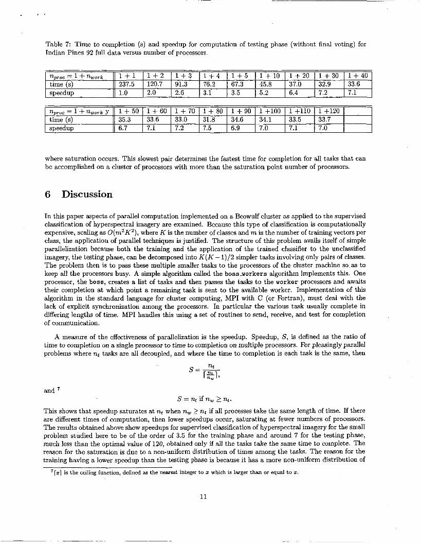
Table 7: Time to completion (s) and speedup for computation of testing phase (without final voting) for Indian Pines 92 full data versus number of processors.

nproc=l+~vorlc 1 + 1 time (s) 237.5 speedup 1.0

1 4 - 2 1 + 3 1 4 - 4 1 + 5 l + l O 1 + 2 0 1 + 3 0 l + 4 0 120.7 91.3 76.2 67.3 45.8 37.0 32.9 33.6 2.0 2.6 3.1 3.5 5.2 6.4 7.2 7.1

where saturation occurs. This slowest pair determines the fastest time for completion for all tasks that can be accomplished on a cluster of processors with more than the saturation point number of processors.

nproc= 1+nwOrlc y 1 + 50 1 + 60

speedup 6.7 7.1 time (s) 35.3 33.6

6 Discussion

1 + 70 1 + 80 1 + 90 1 +lo0 1 +110 1 +120 33.0 31.8 34.6 34.1 33.5 33.7 7.2 7.5 6.9 7.0 7.1 7.0

In this paper aspects of parallel computation implemented on a Beowulf cluster as applied to the supervised classification of hyperspectral imagery are examined. Because this type of classification is computationally expensive, scaling as O(m2K2), where K is the number of classes and m is the number of training vectors per class, the application of parallel techniques is justified. The structure of this problem avails itself of simple parallelization because both the training and the application of the trained classifier to the unclassified imagery, the testing phase, can be decomposed into K ( K - 1)/2 simpler tasks involving only pairs of classes. The problem then is to pass these multiple smaller tasks to the processors of the cluster machine so.as to keep all the processors busy. A simple algorithm called the b o s s s o r k e r s algorithm implements this. One processor, the boss, creates a list of tasks and then passes the tasks to the worker processors and awaits their completion at which point a remaining task is sent to the available worker. Implementation of this algorithm in the standard language for cluster computing, MPI with C (or Fortran), must deal with the lack of explicit synchronization among the processors. In particular the various task usually complete in differing lengths of time. MPI handles this using a set of routines to send, receive, and test for completion of communication.

A measure of the effectiveness of parallelization is the speedup. Speedup, S, is defined as the ratio of time to completion on a single processor to time to completion on multiple processors. For pleasingly parallel problems where nt tasks are all decoupled, and where the time to completion is each task is the same, then

and S = nt if n, 2 nt.

This shows that speedup saturates at nt when nw 2 nt if all processes take the same length of time. If there are different times of computation, then lower speedups occur, saturating at fewer numbers of processors. The results obtained above show speedups for supervised classification of hyperspectral imagery for the small problem studied here to be of the order of 3.5 for the training phase and around 7 for the testing phase, much less than the optimal value of 120, obtained only if all the tasks take the same time to complete. The reason for the saturation is due to a non-uniform distribution of times among the tasks. The reason for the training having a lower speedup than the testing phase is because it has a more non-uniform distribution of

’ r.1 is the ceiling function, defined as the nearest integer to z which is larger than or equal to z.

1, 11

processing times than for testing. If the processing times are ordered from longest to slowest, then roughly the distribution is more non-uniform if the differences in processing times for tasks are greater. Recall that if all the processing times are equal, the speedup saturates only when ntasks = nWorkers. The distribution of task times in descending order for the first thirteen for the training phase, in s, is

7.50 5.79 3.32 1.86 1.85 1.49 0.84 0.74 0.62 0.58 0.58 0.48 0.38

while for the testing phase, in s, it is

31.2 29.5 20.7 15.5 14.7 9.9 8.0 7.0 6.9 6.3 5.8 5.6 4.9.

The steeper drop in processing times for the training phase than testing phase causes a more rapid saturation of speedup at a lower value. Note that the time for longest task for the training phase is 7.5 s which is close to the saturated time of 9 s, while for the testing phase the time of the longest task is 31 s which is close to the saturated time of 33 s The task times are only for the worker performing the task without the overhead of the boss-worker code creating the tasks and managing them.

In conclusion, though the programming burden of using MPI can be substantial, because all the details of the multiple processor synchronization and communication are the responsibility of the programmer, the low cost and ready availability of cluster hardware suggests that for typical hyperspectral scene sizes of the order 1000 x 10000 with numbers of classes of multiples of 10 can be managed. Of note is that it is currently possible to build very inexpensive low-power clusters [9] that could be made portable.

Because results so far for supervised SVM classification can detect subtle class differences, the approach discussed here provides a means to push the use of SVM techniques to much larger scenes and number of classes than are currently performed for hyperspectral imagery. It remains for future work to see how far this approach can more fully exploit the large amount of information contained in hyperspectral imagery with reasonable times for computation.

Acknowledgments

The author is grateful to Chi-Chung Chang and Chih-Jen Lin [5] for making LIBSVM available for im- plementing the SVM pair classification. John Dorband, Josephine Palencia, Udaya Ranawake, and Glen Gardner of NASA/GSFC have provided hardware and software support for the cluster system at GSFC used in this work.

Appendix A Simple example of parallel computation In time step 1 and in parallel let processor p i perform the addition of u1,u2, p2 perform the addition of a3,a4,

. . . p ~ p perform the addition of ~ N - I , U N . In time step 2, let p i add the the result from step 1 to the result from p 2 in step 1, pa add the the result from step 1 to the result from p3 in step 1, . . . PN/4 add the result from step 1 to the result from p ~ / 2 . Continuing like this eventually leads to the last single addition between p i and pa at time step O(ZogzN). Note that we spend a fixed time at each step to pass values between processors, which itself occurs 0 (log2 N ) times.

'Proteus cluster with 14 nodes, (mini ITX boards), power consumption 170 W, peak demand 438 W. Controlling nodes have 256 MB RAM, gigabit ethernet, and a 40 GB hard drive. The NFS server node is similarly equipped. Computational nodes have 256 MB RAM. Peak performance 5.2 GFLP and 10,400 MIPS with 13 computational nodes. Cost w $3000.

12

References [l] R. E. Bellman. Adaptive Control Processes: A Guided Tour. Princeton University Press, Princeton, New Jersey,

U.S.A., 1961. [2] B. E. Boser, I. M. Guyon, and V. N.\apnik. A training algorithm for optimal margin classifiers. In Fifth Annual

Workshop on Computational Learning Theory, pages 144-152. ACM, June 1992. [3] L. Bruzzone and F. Melgani. Classification of hyperspectral images with support vector machines: multiclass

strategies. In Proceedings of SPIE, 2004. [4] G. Camps-Valls, L. G6mez-Choval, J. Calpe-Maravilla, E. Soria-Olivas, J. D. Martin-Guerrero, and J. Moreno.

Support Vector Machines for Crop Classification Using Hyperspectml Data, pages 134 - 141. Springer-Verlag, Heidelberg, October 2003.

[5] Chih-Chung Chang and Chih-Jen Lin. Libsvm - a library for support vector machines. The demo is available from http://vwv.csie.ntu.edu.tw/'cjlin/libsvm/.

[6] C. Cortes and V. N. Vapnik. Support vector networks. Machine Learning, 2O:l-25, 1995. (71 J. E. Devaney, M. Michel, J. Peeters, and E. Baland. Automap: A software tool for the automatic creation of

mpi data structures from user code. Technical report, NIST, April 1997. http: //vwv. it1 .nist .gov/div895/ savg/parallel/.

[SI Ian Foster. Designing and Building Parallel Programs. Addison-Wesley, 1995. [9] Glen Gardner, 2004. http : //members. verizon. net/'vze24qhw/.

[lo] W. Gropp. Tutorial on MPI: The Message Passing Interface. Argonne National Lab., Argonne, Illinois. Available at http://vwv-unix.mcs.adl.gov/mpi/tutorial/gropp/talk.html\#NodeO.

[ll] W. Gropp. Tutorial on MPI: The Message Passing Interface. Argonne National Lab., Argonne, Illinois. See node 87to node 93 inhttp://vvv-unix.mcs.anl.gov/mpi/tutorial/gropp/talk.html\#NodeO.

[12] W. Gropp and E. Lusk. Exercises for the MPI TutoriaL Argonne National Lab., Argonne, Illinois. Available at http://wuv-unix.mcs.anl.gov/mpi/tutorial/mpiexmpl/src/fairness/Cwaitsom%e/solution/.html.

[13] W. Gropp, E. Lusk, and A. Skjellum. Using MPI: Portable Parallel Programming with the Message Passing Interface. MIT Press, 1996. J. A. Gualtieri and S. Chettri. Support vector machines for classification of hyperspectral data. In International Geoscience and Remote Sensing Symposium. IEEE, 2000. J. A. Gualtieri, S. R. Chettri, R. F. Cromp, and L. F. Johnson. Support vector machine classifiers as applied to aviris data. In R. Green, editor, Summaries of the Eighth JPL Airborne Earth Science Workshop:JPL Publication 99-1 7, pages 217-227. Jet Propulsion Laboratory, California Institute of Technology, Pasadena, California, Feb 1999. Available athttp://aviris.jpl.nasa.gov/docs/workshops/99\-docs/toc.htm.

J. A. Gualtieri and R. F. Cromp. Support vector machines for hyperspectral remote sensing classification. In R. J. Merisko, editor, 27th AIPR Workshop, Advances in Computer Assisted Recognition, Proceedings of the SPIE, Vol. 3584, pages 221-232. SPIE, 1998. C.W. Hsu and C. J. Lin. A comparison of methods for multi-class support vector machines. IEEE %ns. on Neural Networks, 13(2):415-425, 2002. G. F. Hughes. On the mean accuracy of statistical pattern recognizers. IEEE Transactions on Information Theory, 14(1):55-63, 1968. T. Joachims. Making large-scale SVM learning practical. In B. Scholkopf, C. Burges, and A. Smola, editors, Advances in Kernel Methods - Support Vector Learning. MIT Press, 1998. Available at http: //vwv-ai . cs . uni-dortmund.de/DOKUMENTE/Joachims-98b.ps.gz.

T. Joachims, 2001. The SVMlight package is written in GCC and distributed for free for scientific use from http: //ais .pd. de/"thorsten/svm-light/ It can use one of several quadratic optimbers. For our application we used the A. Smola's PRLOQO package [26]. L. F. Johnson. Aviris hyperpsectral radiance data from: f981009tOlr-07, 1998. ftp: //makalu. jpl .nasa. gov/ pub/98qlook/1998~lowalt\~index. html.

D. Landgrebe. Indian pines aviris hyperpsectral radiance data: 92av3c, 1992. Available at ftp: //ftp. ecn. purdue.edu/biehl/MultiSpec/92AV3C. ftp://ftp.ecn.purdue.edu/pub/biehl/PC-MultiSpec/ThyFiles.zip. http://aviris.jpl.nasa.gov/ql/list92.html. http://dynamo.ecn.purdue.edu/'biehl/MultiSpec/aviris- documentation. html%.

13

[23] M. Lennon, G. Mercier, and L. Hubert-Moy. Classification of hyperspectral images with nonlinear filtering and

[24] Peter S. Pacheco. Parallel Programming with MPI. Morgan Kaufmann, 1996. http: //nexus. c s .usf ca. edu/

[25] B. Scholkopf, C. Burges, and A. Smola, editors. Advances in Kernel Methods. MIT Press, 1998. [26] A. Smola, 2001. The PRLOQO quadratic optimization package is distributed for research purposes by A. Smola

at ht tp : //m. kernel-machines . org/code/prloqo . t a r . gz.

[27] T. Sterling, D. Savarese, D. J. Becker, J. E. Dorband, U. A. Ranawake, and C. V. Packer. BEOWULF: A parallel workstation for scientific computation. In Proceedings of the 244th International Conference on Parallel Processing, volume I, Architecture, pages 1:ll-14, Boca Raton, Florida, August 1995. CRC Press.

[28] G. Zanghirati and L. Zanni. A parallel solver for large quadratic programs in training support vector machines. Parallel Computation, 29(4):535-551, 2003.

[29] Junping Zhang, Ye Zhang, and Tingxian Zhou. Classification of hyperspectral data using support vector machine. In Proceedings 2001 International Conference on Image Processing, volume 1, pages 882-885, October 2001.

support vector machines. In International Geoscience and Remote Sensing Symposium, 2002.

mpi/.

14