a parallel tabu search algorithm for large traveling ... · a parallel tabu search algorithm for...

DISCRETE APPLIED

ELSEVIER Discrete Applied Mathematics 51 (1994) 243-267

MATHEMATICS

A parallel tabu search algorithm for large traveling salesman problems

C.-N. Fiechter*

Ecole Polytechnique Ft?d&ale de Lausanne, Departement de MathCmatiques, CH-1015 Lausanne, Switzerland

(Received 12 April 1990; revised 16 July 1992)

Abstract

Tabu search is a general heuristic procedure for global optimization which has been successfully applied to several types of difficult combinatorial optimization problems (scheduling, graph coloring, etc.).

Based on this technique, an efficient algorithm for getting almost optimal solutions of large traveling salesman problems is proposed. The algorithm uses the intermediate- and long-term memory concepts of tabu search as well as a new kind of move. Experimental results are presented for problems of 500-100000 cities and a new estimation of the asymptotic normalized length of the shortest tour through points uniformly distributed in the unit square is given.

Finally, as the algorithm is well suited for parallel computation, an implementation on a transputer network is described. Numerical results and speedups obtained show the efficiency of the parallel algorithm.

Key words: Combinatorial optimization; Tabu search; Traveling salesman problem; Parallel algorithms; Transputer

1. Introduction

During the last decade considerable effort has been devoted to solving large combinatorial optimization problems, and in particular the famous traveling salesman problem (TSP). Many heuristic procedures for this problem have been proposed by different authors. The tabu search (TS) technique, developed in the last ten years by Glover [7], differs markedly from most of them by its generality. TS is not specifically designed for one type of problem but is, on the contrary, a general procedure for global optimization that can be easily applied to many types of problems.

*Present address: Department of Computer Science, University of Pittsburgh, Pittsburgh, USA.

0166-218X/94/$07.00 0 1994-Elsevier Science B.V. All rights reserved SSDI 0166-218X(92)00033-1

244 C.-N. Fiechter / Discrete Applied Mathematics 51 (1994) 243-267

In fact, rather than a simple heuristic, TS can be seen as a metaheuristic, i.e., a heuristic method within which a local search heuristic procedure can be used, and which guides this “lower-level” procedure to better solutions. Another main charac- teristic of TS, linked to the latter, is to induce a decomposition of the optimization process into a hierarchy of searches, from the most local to more and more global searches. At each of these levels, TS introduces a kind of memory for guiding the process. Thus, TS looks more like an intelligent search, which may in some sense imitate a human behavior or apply some rules based on artificial intelligence principles, unlike the well-known simulated annealing technique which tries to use an analogy with thermodynamics (see [3]).

In most applications proposed so far, TS was used only at the lowest level, i.e., according to the TS terminology which will be specified in Section 2, as short-term memory. In this simple form it has been very efficient for solving many types of difficult problems (scheduling [17], graph coloring [9], etc.) but has yielded only fair results for the TSP [18]. The heuristic procedure for the TSP proposed in this paper illustrates how TS can be used for guiding the optimization process at a higher level. The significance of our results is amplified because we continue to rely on very simple moves at the lower level.

The problem we are going to consider can be formulated as follows (for a general presentation of the TSP, see [l 11): given a completely connected graph G on n nodes and a symmetric distance function dij = dji that measures the distance from node i to node j, the problem consists in determining a minimal cost cycle that passes, exactly once, through each node of the given graph. For the sake of simplicity, in the numerical experiments to be presented, we concentrate on Euclidean distances. Even with this additional assumption the TSP is known for being NP-hard.

Another point in combinatorial optimization which is receiving an increasing amount of attention is the development of parallel algorithms. We focus here on MIMD (multiple instruction, multiple data stream) parallel computers, in which the different processors are simultaneously allowed to perform different types of instruc- tions on possibly different data (see [S]). In this context, TS used at a high level seems to offer a good framework for parallelism. The general idea is that the local search heuristic used inside TS can be sliced into several independent searches, performed in parallel, without much loss of quality, while TS assures a high global quality of the solution.

In the next section, a brief review of the basic principles of TS is given, with emphasis on intermediate- and long-term memory concepts. The application of these concepts to the TSP is explained in Sections 3 and 4; computational results are presented in Section 5. Finally, Section 6 describes the implementation of the algorithm on a transputer network.

2. Tabu search

2.1. General formulation

The development of TS has brought up many improvements and refinements to the original idea. In this section we will just sketch the general and simplest procedure and

C.-N. Fiechter J Discrete Applied Mathematics 51 (1994) 243-267 245

specify the concepts of short-, intermediate- and long-term memory. For a general presentation of TS with various applications, the reader is referred to [X, lo].

TS is devised for solving combinatorial optimization problems of the general form:

min{ f(s) 1 SEX}, where X is a set of feasible solutions and f a cost function.

TS is an iterative algorithm, which moves step by step from an initial feasible solution toward a solution s* that seeks to minimize h at least approximately. For this we have to define a class of simple modifications that can be applied to a solution in order to move to the next one. We will call M the set of these acceptable modifications and will write s’ = s @ m, m E M, meaning that solution s’ is obtained by applying modification m to solution s. This induces the definition of a neighborhood N(s) of each solution s, which is the set of solutions directly reachable from s by such a modification. It is convenient to represent this by a graph in which each node corresponds to one solution, two nodes s and s’ being connected by an arc (s, s’) if s’ E N(s). The solutions consecutively visited by the search procedure will then form an oriented path in this graph.

At each step of the iterative procedure, the “local” optimization problem min {f(x) 1 x E V* c N(s)} is solved and the move from s to the best solution s’ found in Y* is made, whether f(s’) is better than f(s) or not. Depending on the size of the neighborhood chosen, the local optimization problem can be either solved exactly or approximated by any heuristic procedure.

Up to this point, the algorithm is close to a local improvement technique except that we may move from s to a worse solution s’, and thus may escape from local minima of f, and that moves may be limited to a proper subset V* of the complete neighborhood. The key feature of TS is precisely to forbid moves that would bring the process back to one of the recently visited solutions in order to limit the risk of cycling. For doing this, the last moves and/or the reverse of the last moves may be collected in a list T (tabu list) of forbidden moves. A move remains forbidden only for a fixed number of iterations and so the tabu list T can be represented by a queue: at each iteration, the oldest element (the tail of the queue) will be deleted, and the last modification or its reverse will be added as head of the queue.

In practice, the tabu status is assigned to some constituents ti of moves. Each constituent of forbidden moves is collected in a different list Ti and tabu conditions of the form

ti(m)E z (i = 1, . . . , t)

are introduced. Move m will then be forbidden (tabu) if it satisfies all tabu conditions. The example given in the next paragraph will help to clarify these concepts.

2.2. Short-term memory

The level at which TS is used, and thus the kind of memory it introduces in the optimization process, depends principally on the choice of the moves considered, and hence on the complexity of the subproblem to solve at each step of the procedure. The larger the neighborhood, the more global the search and the higher the level.


Fig. 1. 2-opt moves.

In the TSP for instance, we may consider simple moves like those proposed by Lin and Kernighan [12] in their well-known 2-opt algorithm. These 2-opt moves, as we will call them, consist in the deletion of two edges and their replacement by the two others that rebuild the tour (cf. Fig. 1). Each solution has thus n(n - 1)/2 neighbors and the best move can easily be determined. For defining the tabu conditions, we may introduce, for instance, two tabu lists TO,, and T,, containing the last k edges added to the tour and the last 1 edges removed from the tour, respectively. Constituents of move m are then defined in a straightforward way by letting ti,(m) identify the two added edges and tout(m) the two dropped edges. A move m will then be considered tabu if both tin(m) E T:,, and tout(m) E TO,, (for a complete description of a TS algorithm using such moves, see [7] or [ 181).

These simple moves change the solution only slightly and the best move is very easy to identify, enabling a simple form of TS to guide the optimization process at every basic step of the procedure. In this kind of algorithm, the tabu list is clearly used as short-term memory.

2.3. Intermediate- and long-term memory

When a region (in the sense defined by the low-level neighborhood) gives evidence of containing good solutions, an intelligent procedure should intensify the search in this region. The goal of intermediate-term memory is precisely to allow such an intensification. In TS this can be done by isolating some properties of solutions in the considered region and limiting moves to those conserving these properties. For example, in the TSP, edges incorporated in different good tours are only a small fraction of the entire edge set. To intensify the search around a good solution, we can thus only consider a very limited set of edges, based on those contained in the previous solutions. As the neighborhood is now much smaller, iterations are much faster to execute and the search procedure can examine the region much more thoroughly in a given span of time. Section 3 presents how this concept of intermediate-term memory is used in our algorithm.

Finally, an intelligent search technique should not only focus intensively on regions that contain good solutions previously found but should also try to ensure that no region has been completely neglected. A usual way of seeking diversity in an iterative procedure is to repeat the whole search from several randomly generated initial solutions. However, with such an approach there is no opportunity to learn from the past. The long-term memory function of TS should allow, on the contrary, an “intelligent” diversification of the search by guiding the process to regions that

C.-N. Fiechter 1 Discrete Applied Mathematics 51 (1994) 243-267 241

Initialization: construct (by any heuristic procedure) an initial solution s in X

s* := s (s* = best solution so far) iter := 0 (iterations counter)

q := 0 (tabu lists)

While iter < itermax do iter := iter + 1 intensijication:

find (by a heuristic procedure using simple moves and limited neighborhood)

a best solution s’ around s

if f(s’) < f(s*) then s* := s’

s:= s’ if iter < itermax then diversijcation:

i:= 0 While i < imax do

i:= i + 1

generate a set V* G N(s) of solution x = s @ m such that M is a valid

super-move and at least one tabu condition tj(m) E Tj is violated;

choose (possibly by a heuristic procedure) a best solution s’ in V* if f(s’) -c f(s*) then s* := s’ update tabu lists T,

s:= s’

end

Fig. 2. High-level TS.

markedly contrast with those examined thus far. The objective is to create a function that generates new starting points for the normal search or intensification by purpose- ful instead of random means. One way to implement such a long-term strategy is to use a “high-level” tabu procedure. This long-term TS should introduce into the current solution modifications that greatly change its structure, compared to the defined lower-level neighborhood. This can be done by applying at each step one (or several) super-move(s) that highly differ from those used in normal search and which are unlikely to be realized by simple combinations of lower-level moves. It is clear that, in such a tabu procedure, the tabu list plays the role of long-term memory. Fig. 2 outlines such a high-level TS on which our algorithm is based. How it has been applied to the TSP is described in Section 4.

2.4. Parallel tabu search

In iterative search techniques, and in TS in particular, different types of parallelism may be distinguished [14]. We only consider here two general classes according to the method used for parallelizing moves.

First, the search of the next move to perform can be parallelized. This will generally require the partition of the set of feasible moves in p subsets. Each of these subsets is assigned to one process which computes its best member move. The overall best of these p moves is then determined and applied to the current solution (see [14,17]). This technique requires extensive communication since a synchronization is required


at each step. It is therefore only worth applying to problems in which the search of the best move is relatively complex and time-consuming. As this will generally be the case for super-moves, this kind of parallelism can validly be used in the diversification part of the high-level tabu algorithm.

The second type of parallelism we consider consists in performing several moves concurrently. This can be done by partitioning the problem itself into several independent subproblems. Each of the processes can then apply moves to its assigned subproblem, independently of those made in other subproblems. The global solution is then obtained by combining the “subsolutions”. This method needs no communication or synchronization except for its initialization and for grouping the subsolutions at the end. One can therefore expect a real gain in efficiency by the parallel algorithm even when moves are simple. The problem with this kind of parallelism is that it strongly limits the movement possibilities (between different subproblems) and thus generally induces a loss of quality of the global solution. High-level TS seems particularly well suited to overcome this difficulty: this type of parallelism can be used in the intensification algorithm (in which we want to limit the number of moves considered), ensuring the global quality of the final solution by the diversification procedure (which executes structural modifications affecting the entire problem, and not only one component, with its super-moves).

3. Intensification algorithm

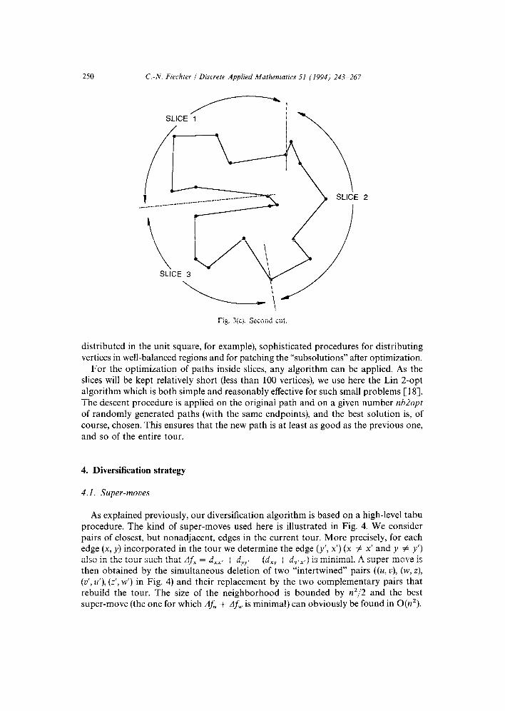
As stated, the intensification strategy should both limit the number of moves to consider at each step and set the stage for parallel computation by allowing concur- rent execution of several moves. The strategy used here is to divide the current tour (around which we want to intensify the search) in k open subtours (slices), each of them having a vertex in common with the two adjacent slices (cf. Fig. 3(a)). The path between these two fixed vertices is then optimized independently one each slice. The complete intensification finally consists of a couple of these cuts with shifted slices, to allow other combinations of edges, particularly around the boundaries between slices.

It is obvious that the length of the tour thus optimized can only be less than (or possibly equal to) that of the original tour. If the structure of this initial tour is not too bad (i.e., if there are not too many intersections between distant portions of the tour, for instance, which should be ensured by the higher-level procedure) then it is likely that the solution obtained will be a very good one.

Since, to optimize a given path, we only have to consider the edges linking the vertices in the slice, the entire set of valid moves is greatly reduced. If the length of the slices is kept constant (i.e., if we accordingly increase the number of slices), the complexity of the intensification procedure is linear in n (the number of nodes of the problem), regardless of the algorithm used for optimizing the slices. Finally, the entire procedure is clearly suited for parallel computing, as optimizations are done completely independently on each slice, and can thus be done concurrently.

It should be noted that this strategy is quite different from that proposed by Karp (see [ll]), as used by Bonomi and Lutton [2], in which vertices are divided in “geographical” regions and which requires, except in special cases (vertices uniformly

C.-N. Fiechter / Discrete Applied Mathematics 51 (1994) 243-267 249

Fig. 3(a). First cut.

SLICE 3

Fig. 3(b). First cut, after optimization of the slices.


Fig. 3(c). Second cut.

distributed in the unit square, for example), sophisticated procedures for distributing vertices in well-balanced regions and for patching the “subsolutions” after optimization.

For the optimization of paths inside slices, any algorithm can be applied. As the slices will be kept relatively short (less than 100 vertices), we use here the Lin 2-opt algorithm which is both simple and reasonably effective for such small problems [lS]. The descent procedure is applied on the original path and on a given number nb2opt

of randomly generated paths (with the same endpoints), and the best solution is, of course, chosen. This ensures that the new path is at least as good as the previous one, and so of the entire tour.

4. Diversification strategy

4.1. Super-moves

As explained previously, our diversification algorithm is based on a high-level tabu procedure. The kind of super-moves used here is illustrated in Fig. 4. We consider pairs of closest, but nonadjacent, edges in the current tour. More precisely, for each edge (x, y) incorporated in the tour we determine the edge (y’, x’) (x # x’ and y # y’) also in the tour such that dfX = d,,, + d,,, - (d,, + d,,,,) is minimal. A super-move is then obtained by the simultaneous deletion of two “intertwined” pairs ((u, v), (w, z), (v’, u’), (z’, w’) in Fig. 4) and their replacement by the two complementary pairs that rebuild the tour. The size of the neighborhood is bounded by n2/2 and the best super-move (the one for which dfu + dfw is minimal) can obviously be found in 0(n2).


Fig. 4. Super-move.

These super-moves correspond to the displacement of a complete portion of the tour from one point to another. This choice is motivated by noting that different good solutions of a same TSP instance generally contain a great proportion of identical sections and differ in the order in which these parts are visited. The chosen super- moves precisely allow such a reordering. It is also worth noting that these super- moves do not rely on the symmetry of the distance function.

With respect to the lower-level neighborhood, such super-moves represent relatively complex modifications. To be obtained at the lower level, a super-move would require a combination of at least four 2-opt moves, two of them introducing edges between vertices of different pairs. This is unlikely if we only consider super-moves that incorporate pairs of edges distant in the tour. Moreover, with the intensification algorithm based on slicing, it is reasonable to assume that the eight vertices directly involved in the super-move will not all be in the same slice and that such a combination will be impossible. On the contrary, by simultaneously affecting different parts of the tour, these super-moves operate with the goal of offsetting the limitation of moves introduced by the intensification procedure and permit the desired structural modifications. To ensure these properties, we only consider super-moves that satisfy

min{d,(u, w), d,(z, u’), d,(~‘, z’), d,(w’, u’)) 3 distmin,

where d,(x, y) is the number of edges between the vertices x and y in the tour. It is clear that other kinds of moves can be considered, alone or in conjunction with

those just described, as a means of improving the diversification procedure. Some experiments have been carried out with simple insert moves, which extract a vertex from one location and reposition it at another. The quality of the results obtained was practically unaffected when these moves were used in addition to the super-moves described, and was somewhat inferior (with an average increase of 1.7% in the solution length) when they were used alone for the diversification. This can be explained by the fact that even though these insert moves are quire different from the lower-level 2-opt moves they do not introduce a true structural modification in the tour.


4.2. Adaptation of the tabu procedure

For the diversification, we want the super-moves to be distributed on the entire graph and not all to be located in the same region (where, for instance, vertices are closer to each other). The tabu list thus should both forbid cycling and favor such a distribution. To obtain this effect, the tabu status will be attached to vertices instead of edges: each time a super-move is performed, the eight vertices primarily concerned (u, O, u’, L“, w, z, w’ and z’ in Fig. 4) are inserted in the tabu list (and, as usual, the eight oldest in the list are removed). A super-move will then be considered as tabu if more than a fixed number nbutabu of its vertices are tabu.

Since for each diversification we will make a relatively large number of super-moves and since the search for the best move becomes rather time-consuming for very large problems, we use the concept of a candidate list [7]. At each step, instead of conserving only the very best nontabu super-move, the nbcand best ones are kept, which is not much more time-consuming. Beginning from the best one, these candidate moves are then successively applied, if they are still valid. Since a reasonable

Input:

D: (n x n) matrix of distances d,, s: current tour (s[i] = vertex visited in (i mod n)th position)

s*: best tour found so far

ICLI: number of candidate super-moves kept at each iteration

nbvtabu: number of vertices that can be tabu in a super-move

T: tabu list of vertices

nb( .): set of the nbneigh closest neighbors of each vertex

f(s) = C:= 1 &lulsru+ 11 (length of tour ~1 l- if xET

c, = 0 if x$T

(tabu status of vertices)

for i:= i to imax do

find ICLl nontabu best candidate super-moves: for each edge (x, y) in s determine edge (y’, x’) in s with

y’ E rib(x)) such that x # x’ and y # y’ and

A&:= d,,, + d,,, - (d,, + d,,,,) is minimal

for each edge (u, U) in s do

for each edge (w, z) between (u, U) and (u’, u’) in s do

if super-move ((u, v), (NJ. z), (v’, u’), (z’, w’)) is valid

and (t. + t, + t,,. + t,, + t, + t, + t,, + t,, < nbvtabu) then

insert it (according to its value AfU + AfW) in

CL (ordered list of candidate super-moves)

for each super-move spm in CL do

if spm is valid then s’ := s @ spm if f (s’) < f (s*) then s* := s’

update tabu list: T:= T + {vertices of spm} - {oldest vertices}

s:= s’

end

Fig. 5. Diversification algorithm.


fraction of these candidate moves will probably be independent, several super-moves will be performed at each iteration, and the time spent for the complete diversification, which requires only a few of these steps, will be greatly reduced. It should be noted that this strategy cannot generally be used in lower-level TS since it does not ensure that the very best move is applied at each step. This presumably is not critical here since we chiefly seek diversification.

Finally, to speed up the search for pairs of closest edges, we only consider, for edge (x, y), those issuing from the &neigh closest neighbors of x. It is indeed likely that the closest edge will be one of these. The set of closest neighbors of each vertex is, of course, computed only once at the beginning of the program. Fig. 5 gives an algorithm featuring the above characteristics.

5. Computational results

The numerical experiments have been mainly carried out on problems with cities uniformly distributed in the unit square. Some tests have also been made on two “classical” problems: the Grotschel’s TSP on 442 points and the 532-city problem solved by Padberg and Rinaldi. All numerical results of the sequential version of the algorithm presented in this section have been obtained on SILICON GRAPHICS stations (1.6 Mflops), using PASCAL language. We will first briefly discuss the choice of the parameters used.

5.1. Choice of parameters

There are several parameters in the algorithm that have to be adjusted. In fact, it appears that there is no need for fine tuning and that the quality of the solutions obtained seems relatively insensitive to their precise values as long as they are chosen in reasonable ranges. Moreover, most of these parameters can be kept constant for problems of different sizes. To determine good values of the parameters, we used a collection of 50 problems of 500 points uniformly drawn in the unit square.

The first parameters that have to be considered are those of the intensification part of the algorithm. As mentioned previously, it seems reasonable to keep the length 2 of the slices constant and to choose consequently their number. As the time spent for the optimization of paths depends on both the number of edges in the slice (A’) and the number of iterations performed (nb2opt), these two parameters have been determined simultaneously. It appears that values of 2 around 70 with nb2opt = A/4 yield good compromises between the quality of the solutions obtained and the time required. Concerning the number of “cuts” performed at each intensification (nbcut), only few improvements are made on a solution after two cuts if the initial solution is not too bad. We therefore always choose nbcut = 2 except for the first intensification, which starts with the solution obtained by the initialization algorithm, for which we used nbcut = 3.

For the diversification step, since we want the modifications to be distributed on the entire graph, the number of super-moves performed should be proportional to n (and hence to the tabu list length 1 Tl). Moreover, it is reasonable to assume that the

254 C.-N. Fiechter 1 Discrete Applied Mathematics 51 (1994) 243-267

number of independent super-moves, which can be found in one search, is also proportional to n. We therefore kept the number of searches (imax) constant and consequently changed the length of the candidate list (ICLl). We found that the algorithm gives good results for numbers of super-moves (at each diversification) ranging from n/50 to n/150, with a tabu list of that same size. In our tests, we always took 1 CL1 = 21 TI and imax = 4, which seems to yield approximately the desired number of super-moves. For nbvtabu (the number of vertices that can be tabu in a super-move), values from 4 to 6 (those allowing one of the two pairs of edges to have already been used) yield similar results; we always took nbvtabu = 5. Finally, we chose nbneigh = 25 and distmin = 25.

5.2. Randomly generated graph

In their classical paper [l], Beardwood et al. have proved that, for the length I* of an optimal tour through n points, which are independently distributed with a probability function ~(xr , x2) in a bounded region A of the Euclidean plan, we have

lim * = y$ j Jm dxl dx,, n+m & A

with probability 1. y is a “universal” constant which has been estimated to y = 0.53. For points uniformly distributed in the unit square this yields

lim ” z 0.749. n+30 &

This value is often referred to as the Hammersley limit. To generate our problems, we used a congruential random generator known for its

good properties, in particular concerning its two-dimensional uniformity [4]. The initial solutions were obtained by the method proposed by Lutton and Bonomi [2]: the unit square is divided in 2” x 2” subregions in which points are randomly connected. The subregions are then connected in a fixed order to obtain the complete tour. It should also be noted that each distance is recalculated whenever used, except during intensification in which all distances between the vertices of a slice are calculated before applying the 2-opt algorithm.

Table 1 presents the average and standard deviation of tour length and CPU time for problems ranging from 500 to 100000 points. Under the numbers of vertices are given the number of problems solved and the size of the tabu list used. The tour lengths shown are the averages of the solutions found after a given number of iterations (in the sense defined by the high-level tabu algorithm of Fig. 2; iteration 0 corresponds to the initial solution). After the last iteration an extra intensification is applied on the best solution found so far. The columns labelled “SDEV” give the standard deviation, on the problem sample, of the tour length and CPU time, respectively.

It should be noted that the CPU time required linearly depends on the number of iterations performed. Fig. 6 shows the average normalized tour length as a function of this number. As usual with TS techniques, the algorithm quickly reaches good solutions and subsequent improvements are more difficult to obtain.


Table 1 Results of the sequential algorithm for problems of 500 to 100000 points

Problem size

No. of Average iterations length (I*)

SDEV length

Average

[*I&

Average CPU SDEV

time (s) CPU time

500

(100 pb, 1 TI = 10)

1000

(100 pb, ITi = 15)

3000

(100 pb, ITI = 35)

5000

(50 pb, / TI = 50)

10000

(50 pb, ITI = 100)

20 000

(20 pb, I TI = 200)

50 000

(10 pb, I TI = 400)

100 000

(5 pb, 1 TI = 800)

0

1 5

10 20 30

0 1 5

10 20 30

0 1 5

10 20 30

0 1 5

10 20 30

0 1 5

10 20 30

0 1 5

10

0 1 5

10

0 1 5

10

37.043 0.8553 1.65662 17.826 0.2688 0.79721 16.972 0.2044 0.75901 16.862 0.1933 0.75411

16.790 0.1946 0.75088 16.744 0.1916 0.74882

69.673 1.1922 2.20325 25.228 0.3348 0.79779 23.817 0.2511 0.75316 23.647 0.2322 0.74779 23.541 0.2243 0.74443 23.491 0.2199 0.74285

106.803 1.0574 1.94995 43.992 0.3229 0.80317 41.002 0.2527 0.74860 40.69 1 0.2431 0.7429 1 40.494 0.2367 0.73932 40.404 0.2341 0.73767

171.988 1.3614 2.43228

56.834 0.2902 0.80375 52.836 0.2312 0.74722 52.414 0.2237 0.74125 52.176 0.2390 0.73788 52.067 0.2385 0.73634

180.901 0.8861 1.80901 79.802 0.2965 0.79802 74.520 0.2221 0.74520 73.875 0.2176 0.73875 73.527 0.2025 0.73527 73.380 0.2013 0.73380

344.244 1.3346 2.43417 113.639 0.3522 0.80355 105.371 0.2210 0.74508 104.389 0.1849 0.73814

443.927 0.7500 1.98530 177.123 0.3094 0.79212 166.450 0.1875 0.74439 164.79 1 0.1822 0.73697

851.165 1.268 2.69162 252.365 0.154 0.79804 236.103 0.270 0.74662 233.387 0.122 0.73803

2 0.03 13 0.12 47 0.36 90 0.66

176 1.34 269 2.20

4 0.06 28 0.26 98 0.82

185 1.55 360 3.04 551 4.66

13 0.06 86 0.38

309 1.34 588 2.70

1145 5.02 1750 7.91

28 0.12 130 0.35 455 1.87 860 4.35

1668 8.61 2543 12.28

41 0.96 259 2.32 969 11.18

1852 19.82 3617 38.08 5527 57.15

117 0.29 736 1.03

2290 8.15 4531 16.06

231 0.43 1876 6.42 6318 42.81

12639 69.41

720 5.80 4723 14.58

17003 195.35 32 099 276.72


0.77 -

-0

w .- Y??

0.75 -

E 8 Z 0.74 -

0

0.78 -

0.77 -

-0

8 .- a

0.75 -

E 5 Z 0.74 -

5 10 15 20 25 3’0

Number of Iterations

0.73 3 0 2 4 6 8 10

Number of Iterations

Fig. 6. Convergence of the average normalized tour length

It is also clear that the average normalized length decreases with the problem size. Fig. 7 illustrates this point by giving the lengths of the solutions after 30 iterations as

a function of the root of the problem size, as well as the regression line 1 = a + b&. As suggested in [15], this can be used for estimating the performance of the algorithm.


40 60 80 100

w@)

Fig. 7. Tour lengths after 30 iterations.

We have here a = 0.43 and b = 0.7298 (with a coefficient of determination R2 =

0.9999), which favorably compares with the values obtained with other heuristics. For instance, with the 3-opt algorithm, the best one tested in [15], Ong and Huang obtained a = 0.55 and b = 0.7425 using problems ranging from 30 to 200 nodes. The slope b of the regression line is also a good estimator of the asymptotic limit

/It_, = ~4. From the regression analysis we can draw ptsp d 0.731 (and y 6 0.517) at the 0.01 level. This estimation is close to that made by Ong and Huang and is 2.5% lower than the Hammersley limit.

It is also worth noting that the CPU time required for a given number of iterations varies like O(n’.‘) for the problem sizes considered. This value follows from the mixing of the different complexities of the two steps performed at each iteration. As mentioned previously, the complexity of the intensification is indeed linear in n if the number p of slices is increased as a function of n, whereas that of the diversification is in O(n’).

To our knowledge, only a few results have been published on very large TSPs. Using simulated annealing, Troyon [IS] solved a lOOO-vertex problem and obtained a normalized length of 0.755 in 953 s (on a VAX 8600). It is worth noting that, for the same problem, he obtained 0.798 in 4 h with a “low-level” tabu algorithm. In [2], Lutton and Bonomi proposed an extended Metropolis algorithm in which the unit square is divided in a large number of subregions and only moves exchanging edges of neighboring subregions are considered. With this improved simulated annealing, they solved problems up to 10000 points. They presented a solution of one lOOOO-vertex problem of length 76.3 obtained in 3500 s (on a Honeywell Bull DPS8). With a more recent version of this algorithm, Lutton [13] solved a lOOOO-vertex problem and obtained 73.36 after 50 million iterations (lh20 on a SUN SPARC station). The solution, of length 72.95, obtained for this problem by our high-level tabu algorithm is given in Fig. 8. We unfortunately do not know any published results for larger problems.

258 C.-N. Fiechter 1 Discrere Applied Mathematics 51 (1994) 243-267

Fig. 8. Solution after 30 iterations of Lutton’s 10 OOO-vertex problem (tour length = 72.95).

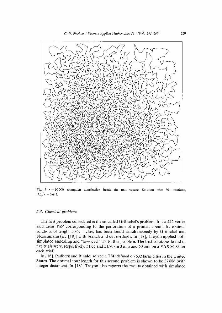
Finally, Fig. 9 presents the solution found for a problem in which points are independently distributed in the unit square with a nonsymmetrical triangular distribution along both axes:

:

8x, 0 < x < l/4,

P(XI>%) =f(XI)“IW); f(x) = #U - $2 l/4 G x G 1,

0, elsewhere,

which gives

lim * = $y$ &

z 0.65. n+Cc

The quality of the solution obtained shows that the performance of the algorithm does not significantly depend on the uniform distribution of points.

C.-N. Fiechter 1 Discrete Applied Mathematics 51 (1994) 243-267 259

Fig. 9. n = 10000; triangular distribution inside the unit square. Solution after 30 iterations,

l*/$ = 0.645.

5.3. Classical problems

The first problem considered is the so-called Griitschel’s problem. It is a 442-vertex Euclidean TSP corresponding to the perforation of a printed circuit. Its optimal solution, of length 50.67 inches, has been found simultaneously by Griitschel and Fleischmann (see [lS]) with branch-and-cut methods. In [lS], Troyon applied both simulated annealing and “low-level” TS to this problem. The best solutions found in five trials were, respectively, 51.65 and 51.70 (in 3 min and 50 min on a VAX 8600, for each trial).

In [16], Padberg and Rinaldi solved a TSP defined on 532 large cities in the United States. The optimal tour length for this second problem is shown to be 27686 (with integer distances). In [18], Troyon also reports the results obtained with simulated


Table 2

Results for the “classical” problems

Number of Average SDEV Average CPU SDEV iterations tour length length time (s) CPU time

Padberg 0

Rinaldi 1

(I Tl = 15, [CL1 = 30) I:,

20

30

Griitschel 0

(I TI = 15, 1

lCLl=20) 5

10

20

30

30610.7 324.76 26 29 090.3 214.36 36 28 374.0 132.66 67 28 230.7 117.30 106 28 142.1 113.98 183 28 090.2 123.68 267

58.092 0.7901 15 54.450 0.6181 25 52.020 0.3133 56 51.707 0.2221 94 51.533 0.2013 171 51.458 0.1719 254

0.10

0.23

0.58

1.17

1.80 2.61

0.01

0.11

0.46

0.68

1.29

2.04

Optimal Shortest tour Longest tour

solution obtained obtained

Padberg-Rinaldi 27 686 27 839 28 422 Grotschel 50.67 51.10 51.94

annealing and “low-level” TS (using truncated distances for which the optimal solution is 27 424). The lengths of the solutions found were, respectively, 28 418 and 29011.

Table 2 presents the results obtained for both problems with the high-level tabu algorithm. The initial solutions (iteration 0 in the table) were obtained using a random insertion procedure (see [ll]). For each problem, the algorithm has been applied on 100 different initial solutions. Clearly, the results are quite comparable to those obtained with simulated annealing and seemingly better than those of low-level TS. Moreover, the standard deviation obtained and the difference between the smallest and the largest tour found indicate that the algorithm is not too sensitive to the quality of the initial solution. Fig. 10 gives the best solutions obtained for the two problems.

6. Parallel algorithm

As mentioned earlier, two different types of parallelism can be used in the high-level tabu procedure. For the intensification part of the algorithm several movements can be concurrently applied on different slices of tour, whereas for the diversification part it is the search of the best moves that can be done in parallel.


Fig. 10(a). Best solution obtained by the high-level TS algorithm for Padberg and Rinaldi’s problem.

6.1. Parallelism for the inter@ication

The principle of the intensification based on the independent optimization of slices of the current tour induces a natural division of the work among different processes. However, in general, the number of slices will be too large to assign each of them to a different processor (for n = 10000 we used, for instance, 140 slices). Each process therefore handles an equal portion of the tour, which is in turn divided into smaller slices. The complete intensification is then performed as follows:

_ Each process divides its portion of the tour into slices and sequentially optimizes them (as in the sequential algorithm).

_ Between two consecutive cuts, the tour is shifted: each process sends to its successor (the one that handles the next portion of the tour) the path it has found

262 C.-N. Fiechier / Discrete Applied Mathematics 51 (1994) 243-267

Fig. 10(b). Best solution obtained by the high-level TS algorithm for Griitschel’s problem

among the last shift vertices of its tour portion and receives the corresponding information from its predecessor.

_ At the end of the intensification (after a fixed number of cuts), the optimized portions are collected and redistributed to all processes such that they all have the entire tour for the next iterations. Clearly, the algorithm is very well suited for implementation on a MIMD parallel computer, since for each cut there is only one synchronization between adjacent processes, with little information to transmit.

6.2. Parallelism for the diversljication

To allow the search of the next super-move to perform to be done in parallel, the set of the feasible moves has to be divided into subsets in which each process can search its candidates. The most natural way of doing this for the TSP is to partition the city


set among the processes. The search of the candidate super-moves can then be done as follows:

- For every edge in the current tour issuing from one of its vertices, each process determines the closest edge also in the tour (using, as in the sequential version, lists of closest neighbors for the vertices).

- The pairs thus obtained are collected and redistributed to all processes. - Every process then searches a fixed number of candidate super-moves consider-

ing only those for which the first vertex (u in Fig. 4) belongs to its own subset of vertices.

~ The candidate “sublists” thus created are again collected and redistributed to the processes, which all build the final candidate list (by merging the sublists) and apply the moves. In addition to this, during the initialization part of the algorithm, the sets of closest neighbors have to be created. It is clear that each process has to compute and store only those attached to its vertices. We therefore have a distribution of both computational work and storage requirement.

The only drawback of this parallel algorithm is that two synchronizations between all processes are required for each search of candidates. Let us, however, notice two things. First, by assigning the same number of cities to each process, we can expect them to do approximately the same amount of work between synchronizations. The whole diversification tends therefore to work in a near-synchronous way. Secondly, we assume that the work made twice (the execution of super-moves in particular) and the time required by communications will remain small with regard to the amount of work that is really performed concurrently between synchronizations.

6.3. Implementation of the parallel algorithm

The algorithm has been implemented on a network of transputers in OCCAM language. A transputer is a microprocessor-on-a-chip specifically designed to build multiprocessor MIMD machines with distributed memory. Each transputer is connected to its own local memory and, through special bidirectional links, directly to up to four other transputers. Any communication network with a maximum degree of no more than four can be easily set up by connecting the links of adjacent processors.

Although other network topologies may be considered, we used a ring structure in which each processor is directly connected to one predecessor and one successor. On each processor runs one of the previously described “node” processes. In addition, one processor handles a “master” process, as illustrated in Fig. 11. The only work of this process is to initiate the execution of the algorithm and to keep the best solution found up to date.

It should be noted that this processor configuration is ideal for the intensification,

in which only directly connected processors have to communicate. Moreover, since the information is equally distributed among all processors, this network topology is also adequate for collecting and redistributing this information to all processes. This can be done indeed in p consecutive steps during which every process simultaneously


Fig. 11. Network configuration for the parallel algorithm.

sends to its successor a pth of the complete information. If the transmission time of a message is considered to be a linear function of its size, then the time required for the complete collecting and redistribution does not depend on the number of processors.

6.4. Computational results

The parallel algorithm has been tested with different numbers of processors for three problem sizes: 500,300O and 10 000 vertices. For each size and configuration, the procedure has been applied on 10 randomly generated problems.

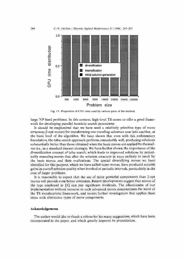
As both the partition of the tour into slices and the candidate lists created depend on the number of processes, the algorithm does not choose exactly the same moves in the different configurations. Nevertheless, the quality of the solutions obtained after a fixed number of iterations is virtually unaffected. We therefore consider here only the CPU times. Fig. 12(a) gives the average CPU time used for the different problem sizes as a function of the number of processors. The corresponding speedups, which are the ratios between the time required by the algorithm executed on one and p transputers, are given in Fig. 12(b). Clearly, even for rather large numbers of processors the speedups are close to optimal. That the speedup is slightly lower for n = 10 000 than for smaller problems can be explained by the fact that the proportion of time spent for the diversification increases with the problem size (cf. Fig. 13). Since the parallelism is less efficient in this part of the algorithm than in the intensification part, the overall efficiency tends to decrease.


0 2 4 6 8 10 12 14 16 18 20 22 24

Number of Processors

18-

16 -

14 -

a 12- 3

$ IO-

% 8- ul

6-

4-

2-

01~,.,.1~,~,.,~,~,.,.,.,.,~ 0 2 4 6 8 1012141618202224

Number of Processors

Fig. 12. Average CPU time and speedup of the parallel algorithm

7. Conclusion

In this paper, we illustrated how TS can be used for guiding an optimization process at a high level rather than at every basic step of the search. The results presented for the TSP showed that this method can efficiently be used for obtaining near-optimal solutions of very large problems. In the foreseeable future, parallel computers will certainly grow fast in power and will become an interesting vehicle in the solving of


0.0 500 1000 3000 5000 10000 20000 50000 100000

Problem size

Fig. 13. Proportion of CPU time used by various parts of the method.

large NP-hard problems. In this context, high-level TS seems to offer a good framework for developing parallel heuristic search procedures.

It should be emphasized that we have used a relatively primitive type of move structure (2-opt moves) for transforming one traveling salesman tour into another, at the basic level of the algorithm. We have shown that even with this rudimentary foundation, the tabu search approach performs remarkably well, producing solutions substantially better than those obtained when the basic moves are applied by themsel- ves (i.e., in a standard descent strategy). We have further shown the importance of the diversification concept of tabu search, which leads to improved solutions by period- ically executing moves that alter the solution structure in ways unlikely to result by the basic moves and their evaluations. The special diversifying moves we have identified for this purpose, which we have called super-moves, have produced notable gains in overall solution quality when invoked at periodic intervals, particularly in the case of larger problems.

It is reasonable to expect that the use of more powerful components than 2-opt moves will provide even better outcomes. Recent developments suggest that moves of the type employed in [6] can pay significant dividends. The effectiveness of our implementation without recourse to such advanced moves demonstrates the merit of the TS metaheuristic framework, and invites further investigation that applies these ideas with alternative types of move components.

Acknowledgements

The author would like to thank a referee for his many suggestions, which have been incorporated in the paper, and which greatly improve its presentation.

C.-N. Fiechter / Discrete Applied Mathematics 51 11994) 243-267 261

References

[l] J. Beardwood, J.H. Halton and J.M. Hammersley, The shortest path through many points, Proc.

Cambridge Philos. Sot. 55 (1959) 2999327.

[Z] E. Bonomi and J.L. Lutton, The N-city travelling salesman problem: statistical mechanics and the

Metropolis algorithm, SIAM Rev. 26 (1984) 551-568.

[3] R.E. Burkard and F. Rendl, A thermodynamically motivated simulation procedure for combinatorial

optimization problems, European J. Oper. Res. 17 (1984) 169-174.

[4] G.S. Fishman and L.R. Moor, A statistical evaluation of multiplicative congruential random number

generators with modulus 231 - 1, J. Amer. Statist. Assoc. 77 (1982) 1299136.

[S] M.J. Flynn, Very high-speed computing systems, Proc. IEEE 54 (1966) 19Oll1909.

[6] M. Gendreau, A. Hertz and G. Laporte, New insertion and postoptimization procedures for the

traveling salesman problem, CRT-708 Centre de Recherche sur les Transports, Universite de

Montreal, Montreal, Canada (1991).

[7] F. Glover, Tabu search-Part 1, ORSA J. Comput. 1 (1989) 190-200.

[S] F. Glover, E. Taillard and D. de Werra, A user’s guide to tabu search, ORWP 92/01, DMA, Ecole

Polytechnique Fiderale de Lausanne, Lausanne, Switzerland (1992).

[9] A. Hertz and D. de Werra, Using tabu search technique for graph coloring, Computing 39 (1987)

3455351.

[lo] A. Hertz and D. de Werra, The tabu search metaheuristic: how we used it, Ann. Math. Artificial

Intelligence 1 (1990) 111-121.

[ll] E.L. Lawler, J.K. Lenstra, A.H.G. Rinnooy Kan and D.B. Shmoys, eds., The Traveling Salesman

Problem: A Guided Tour of Combinatorial Optimization (Wiley, New York, 1985).

[12] S. Lin and B.W. Kernighan, An effective heuristic algorithm for the travelling salesman problem,

Oper. Res. 21 (1973) 498516.

[13] J.L. Lutton, Private communication, Centre National d’Etudes des Telecommunications, Issy Les

Moulineaux, France (1990). [14] Th. Mohr, Parallel tabu search for the graph coloring problem, ORWP 88/l 1, DMA, Ecole Polytech-

nique Fed&ale de Lausanne, Lausanne, Switzerland (1988).

[15] H.L. Ong and H.C. Huang, Asymptotic expected performance of some TSP heuristics: an empirical

evaluation, European J. Oper. Res. 43 (1989) 231-238.

1161 M. Padberg and G. Rinaldi, Optimization of a 532~city symmetric traveling salesman problem by

branch and cut, Oper. Res. Lett. 6 (1987) 1-7.

[17] E. Taillard, Parallel taboo search technique for the jobshop scheduling problem, ORWP 89/l 1, DMA,

Ecole Polytechnique Fed&ale de Lausanne, Lausanne, Switzerland (1989).

1181 M. Troyon, Quelques Heuristiques et Resultats Asymptotiques pour trois Problemes d’optimisation

Combinatoire, These No. 754, Ecole Polytechnique Fed&ale de Lausanne, Lausanne, Switzerland

(1988).

a parallel tabu search algorithm for large traveling ... · a parallel tabu search algorithm for...

Documents