Munich Personal RePEc Archive

A partial differential equation to express

a business cycle :an implication for

Japan’s law interest policy

Kuriyama, Akira

14 March 2011

Online at https://mpra.ub.uni-muenchen.de/35166/

MPRA Paper No. 35166, posted 03 Dec 2011 17:59 UTC

A Partial Differential Equation to Express a Business Cycle:

Implications of Japan’s Low Interest Rate Policy

Author’s name: Akira KURIYAMA

Author’s affiliation: Sumida Co., Ltd.

E-mail address: kuriyama@tbz.t-com.ne.jp

Address for manuscript correspondence: 1-15-13 Hisinuma, Chigasaki City, Kanagawa, Japan

Phone: 0467-51-8849

1

Abstract

This study presents an equation of income derived from the Keynesian IS curve and the

consumption Euler equation that explains the business cycle. Drawing on multi-period data

from Japan, the model confirms the conventional wisdom that the appropriate policy response

to an inflationary gap is to increase the interest rate when economic growth accelerates and

decrease it when growth decelerates. However, the model indicates that to stabilize a

deflationary gap, policymakers should decrease the interest rate when growth accelerates and

increase it when growth decelerates. This prescription defies generations of conventional

wisdom but fits the historical data remarkably well.

(JEL Nos. E32, E52)

Keywords:

1. Consumption Euler equation

2. Business Cycle

3. Capital

4. Interest rate

5. Elasticity of intertemporal substitution

6. Dynamic optimization problem

7. Variable separation method

8. Income elasticity of capital

9. Japan

10. Financial policy

Introduction

Thirty years ago, businesspeople and policymakers worldwide might have been reading

a book to answer the question How can we become like Japan? Presently, they are more likely

to ask, “How can we avoid becoming like Japan?” This study answers the latter question and

argues that Japan’s adoption of a low interest rate policy following the burst of the bubble

economy has been the major reason for its inability to escape deflation.

Policymakers’ doctrinaire response to a deflationary gap is to reduce interest rates in

hopes of stimulating investment and escaping stagnation. Arguably, this response is based on a

fundamental misconception. During a period of deflation, an economy inherently must suffer

from productive overcapacity. If so, should you not discourage investment? When investment

brings a higher interest rate, I presume that you achieve a higher growth rate.

2

What is needed is a reconsideration of previous equations of national income and theories of

the business cycle. This paper proposes the following equation and discusses its implications:

dt

drdt

Yd2

2

(constant) Y (income), r (interest rate), t (time) (1-1)

Section 2 explains how this equation is derived. Section 3 organizes assumptions of this

theory. Section 4 solves the equation, and Section 5 calculates the value of α. Section 6

provides statistical proof, and Section 7 considers implications of the theory for financial

policy. Section 8 presents the conclusion.

2. Derivation of the Equation

This section presents two ways of deriving Eq. (1-1): using the Old Keynesian IS curve

and the consumption Euler equation familiar to New Keynesians. We begin with the Old

Keynesian IS curve.

First, assume that the macro-economy model of Japan resembles the following, which

includes credible figures for ease of illustration:

(trillion yen, interest rate is expressed in percent):

Consumption function YC 8.030 … (2-1)

Investment function rI 375 … (2-2)

Income balance equation ICY … (2-3)

We derive the IS curve from the following assumptions:

Substituting (2-1) and (2-2) into (2-3):

rYY 3758.030

rY 31052.0

rY 15525 … (2-4)

Eq. (2-4) is the Old Keynesian IS curve. The IS curve can be expressed as a deferential

equation as below. Differentiating both sides of (2-4) with respect to r,

15dr

dY

when r ＝0, 5250 Y .

It is more generally expressed as the following equation:

3

dr

dY (constant)… (2-5)

This means that IS curves can be rewritten universally as equations of the type expressed in (2-

5).

We differentiate (2-5) with respect to t and express it as α (constant) and find α = 0 in this case.

In other words:

drdt

Yd2

(constant) … （2-6)

Solving (2-6) as a partial differential equation and calculating the value of α yields

0 .

Rewriting the equation for ease of solution:

dt

drdt

Yd2

2

(constant) … (2-7）

Next, we consider the derivation of Eq. (1-1) based on micro-economic theory

consistent with i New Keynesian ideas.

Household utility is defined below. First,

11),(

11

tt

tt

mcmcU , （2-8）

where U is household utility, tc is consumption in t, and tm is the quantity of money

held by households. Then utility is

1

1

tm.

There are two parameters, and . expresses relative risk aversionii and is defined in (2-9)

0c

tcc

U

CU … （2-9）

cU and ccU are the first- and second-order derivatives, respectively, of U with respect to C.

The reciprocal is the elasticity of intertemporal substitution:

0C

1

ｔcc

c

U

U

… (2-10)

This definition plays an important role later.

The limiting condition is

111 B)1()B)(1( ttttttt miCm ＋　

1,1 ,B m

4

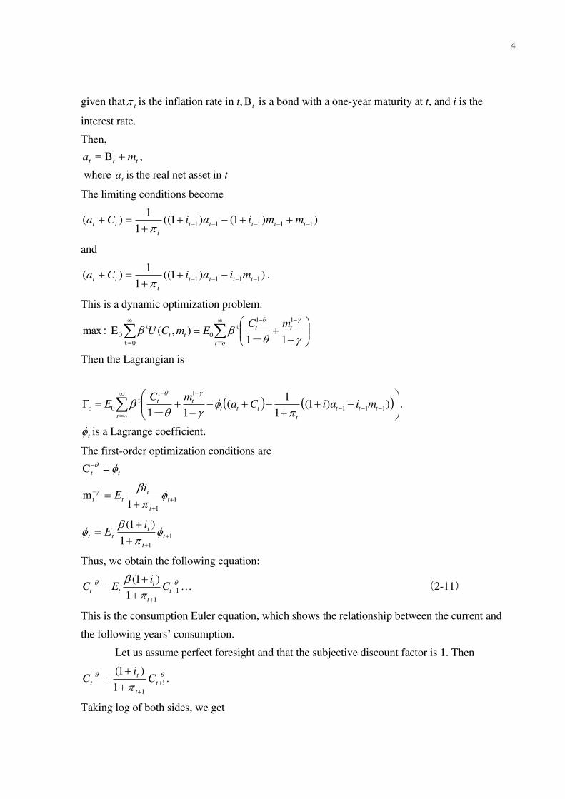
given that t is the inflation rate in t, 　tB is a bond with a one-year maturity at t, and i is the

interest rate.

Then,

ttt ma B ,

where ta is the real net asset in t

The limiting conditions become

))1()1((1

1)( 11111

ttttt

t

tt mmiaiCa

and

))1((1

1)( 1111

tttt

t

tt miaiCa

.

This is a dynamic optimization problem.

1１－),(E：max

11

＝

ｔ0

0 ｔ

ｔ０

tt

ot

tt

mCEmCU

Then the Lagrangian is

))1(1

1(

1１－111

11

＝

ｔ0o ttt

t

ttttt

ot

miaiCamC

E

.

t is a Lagrange coefficient.

The first-order optimization conditions are

tt C

1

11m

t

t

t

tt

iE

1

11

)1(

t

t

t

tt

iE

Thus, we obtain the following equation:

1

11

)1(t

t

ttt C

iEC … （2-11）

This is the consumption Euler equation, which shows the relationship between the current and

the following years’ consumption.

Let us assume perfect foresight and that the subjective discount factor is 1. Then

!

11

)1(t

t

t

t Ci

C .

Taking log of both sides, we get

5

))1()i１＋(in( 1

11 tttt ininCinC

.

So we assume the following relationships:

)i1(in tti

)１＋in( 11 tt

Then

)( 1

11 tttt iinCinC

)(1

1 tt

t

t

iC

dtdC

… (2-12)

New Keynesians construct their models on the bold assumption that Y = C. Because their

models do not include capital, their assumption does not fit my model. Therefore, I assume

propensity to consume is constant (c).

If c is constant, by differentiating c with respect to t , we find that the value of c' is 0.

02

t

tt

tt

Y

dtdY

Cdt

dCY

c .

Then

t

t

t

t

C

dtdC

Y

dtdY

… (2-13)

Substitute (2-13) into (2-12)

)(1

1 tt

t

t

iY

dtdY

… (2-14)

Then we substitute (2-10) into θ:

)( 1 tt

tcc

c

t

t

iCU

U

Y

dtdY

cY

C

t

t

6

)()( 11 tt

cc

ctt

tcc

tct icU

Ui

CU

YU

dt

dY

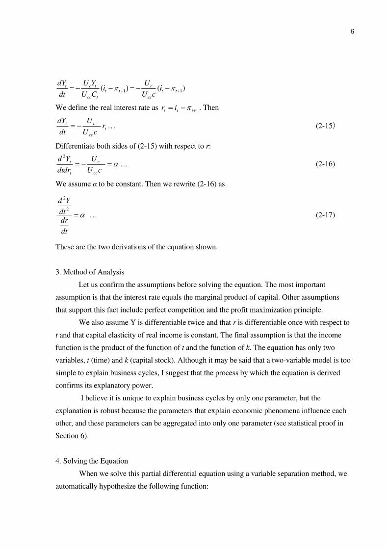
We define the real interest rate as 1 ttt ir . Then

t

cc

ct rcU

U

dt

dY … (2-15）

Differentiate both sides of (2-15) with respect to r:

cU

U

dtdr

Yd

cc

c

t

t

2

… (2-16)

We assume α to be constant. Then we rewrite (2-16) as

dt

drdt

Yd2

2

… (2-17)

These are the two derivations of the equation shown.

3. Method of Analysis

Let us confirm the assumptions before solving the equation. The most important

assumption is that the interest rate equals the marginal product of capital. Other assumptions

that support this fact include perfect competition and the profit maximization principle.

We also assume Y is differentiable twice and that r is differentiable once with respect to

t and that capital elasticity of real income is constant. The final assumption is that the income

function is the product of the function of t and the function of k. The equation has only two

variables, t (time) and k (capital stock). Although it may be said that a two-variable model is too

simple to explain business cycles, I suggest that the process by which the equation is derived

confirms its explanatory power.

I believe it is unique to explain business cycles by only one parameter, but the

explanation is robust because the parameters that explain economic phenomena influence each

other, and these parameters can be aggregated into only one parameter (see statistical proof in

Section 6).

4. Solving the Equation

When we solve this partial differential equation using a variable separation method, we

automatically hypothesize the following function:

7

Y ＝ Y (t, k) ＝ P (t) Q (k)… (4-1)

Therefore, Y is a function of t (time) and k (capital), which is a product of P (t) (price) and Q

(k) (quantity).

First, let us differentiate Y with respect to t once,

)()()()( kQtPkQtPdt

dY .

Then we differentiate Y a second time.

)()()()()()()()(2

2

kQtPkQtPkQtPkQtPdt

Yd

)()()()(2)()( kQtPkQtPkQtP … (4-2)

2

2

2

2

2

)(2)(

dt

dk

k

QtP

dt

dk

k

Q

t

PkQ

t

P … (4-3)

The interest rate is equal to the marginal product of capital (k

QtP

dk

Ydr

)( ).

Therefore,

2

2

2

2

)(k

QtP

dk

Yd

dkdk

dYd

dk

dr

… (4-4)

When we differentiate k

QtP

dk

Ydr

)( with respect to t, we get the denominator of (1-1) as

follows:

dt

dk

k

QtP

k

Q

t

P

dt

rd2

2

)(

…. (4-5)

From (4-3) and (4-5), (1-1) becomes

dt

dk

k

QtP

k

Q

t

P

dt

dk

k

QtP

dt

dk

k

Q

t

PkQ

t

P2

22

2

2

2

2

)()(2)(

k

Q

t

P

dt

dk

k

Q

t

PkQ

t

P

2)(

2

2

＝2

2

2

2

2

)()(

dt

dk

k

QtP

dt

dk

k

QtP

dt

dk

k

Q

t

PkQ

t

P2)(

2

2

＝

dt

dk

dt

dk

k

QtP

2

2

)( .

If t

oePtP)( , so

t

P

t

P

2

2

.

8

Furthermore, we substitute dt

dkfor b．

Then

b

k

QkQ

t

P2)( ＝ bb

k

QtP

2

2

)(

)(2)(

2

2

kQbk

Q

bbk

Q

tP

t

P

(Constant)… (4-6)

Therefore,

)(tPt

P …. (4-7)

bbk

Q

2

2

＝ )(2 2kQb

k

Q … (4-8)

From (4-7) we derive

t

oePtP)( … （4-9）

From (4-8) we derive

0)()2( 2

2

2

kQk

Qb

k

Qbb .

Therefore,

0)2( 2 QQbQbb .

This is a second-order linear differential equation. The characteristic equation is therefore

0)2( 22 bbb .

The basic solution is determined by

bb

bbbb

2

)(4)2()2( 222

＝ bb

b

2

)2( … (4-10)

b

… (4-11)

b

… (4-12)

The content of the radical sign is

)4444(4)2( 2222222bbbbbbb 22

The general solution follows.

9

If D ＝ 0

)exp()exp()( 21 kb

Ckb

CkQ

… (4-13)

If D = 0

))(2

)2(exp()()( 21 k

bb

bkCCkQ

… (4-14)

If D ＝ 0 ,

))(2

sin())(2

cos()()(2

)2(exp()( 21 k

bbCk

bbCk

bb

bkQ

… (4-15)

From (4-1), (4-9), (4-13), (4-14), and (4-15) we find the following:

When D = 0

)exp(),( 1 kb

tCktY

… (4-16)

or

)exp(),( 1 kb

tCktY

… (4-17)

When D = 0 , it means that either 0 or 0 .

Then if 0 ,

))(2

)2(exp()(),( 21 k

bb

bkCCktY

… (4-18)

)exp()(),( 21 kb

tkCCktY

… (4-19)

If 0 , from (4-9) and (4-19), we find

Y (t,k)＝ )( 321 kCCP .

Thus, Y is a primary function of k.

If D = 0 ,

10

))(2

sin())(2

cos()()(2

)2(exp(),( 321 k

bbCk

bbCk

bb

btPktY

… (4-20)

5. Value of α

In this section, we consider the value of α.

From (4-1),

)P(t)Q(k)ｋ,( tY … (4-1)

So from (4-9) and (4-10), we can divide (4-1) into two functions, (5-1) and (5-2), as below.

t

oePtP)( … (5-1)

kBek

bb

bBkQ

))(2

)2(exp()( … (5-2)

：)(2

)2(

bb

b

α is the quotient of (4-3) divided by (4-4). Therefore, α is

)(

))(2(

2

222

0

02

2

dt

dkdt

dk

dt

dk

Be

Be

eP

eP

dt

drdt

Yd

k

kt

t

)(

)(

))(( 2

2

2

dt

dk

dt

dkdt

dk

dt

drdt

Yd

… (5-3)

If

b

… (5-4),

then (5-3) is represented below.

0)(

)()(2

2

bb

bbdt

dk

dt

drdt

Yd

・・・ (5-4)

In Section 6, the statistical analysis shows that Japan has an equation of income such as

in (4-17).

11

)exp(),( 1 kb

tCktY

… (4-17)

Eq. (5-4) indicates that 0 . This implies that if α does not exist, the value of its mean is 0,

and that of its variance is huge. I calculate the actual value in Section 6. Indeed, the variance is

large, but its mean does not equal 0. Thus, I conclude that α exists. This means that when the

correct investment is implemented, the acceleration of income and the fluctuation of the interest

rate will cease, and the economy will have reached a new equilibrium.

Therefore, in the case where D = 0 , Eq. (4-19) shows equilibrium income at that

time on the condition that 0 .

)exp()(),( 21

*k

btkCCktY

… (4-19)

6. Statistical Proof Using Data

In this section, we verify that the equation solved in Section 4 can be reliably applied to

actual cases. First, we consider (4-17).

)exp(),( 1 kb

tCktY

… (4-17)

Putting both sides into a natural logarithm,

kb

tBktinY

0),( …(6-1) ( 10 inCB ).

Equation (6-1) shows that the logarithm value of the nominal GDP can be expressed as

a linear regression model of time (t) and capital (k). Therefore, we fix 1980 as a standard and

conduct a regression analysis on the nominal GDP shown in Reference List 1 by t (1980 as 1)

and k. The result is as follows.

Coefficient of determination: 0.89216685

Adjusted coefficient of determination by degree of freedom: 0.883872

12

Table I Results of Analysis①

Coefficient Standard Error t P-value

0B 4.90583638 0.1397002 35.1169 1.9E-23

1B −0.0499785 0.0133574 −3.74164 0.00091

2B 0.00234751 0.0004156 5.648127 6.1E-06

13

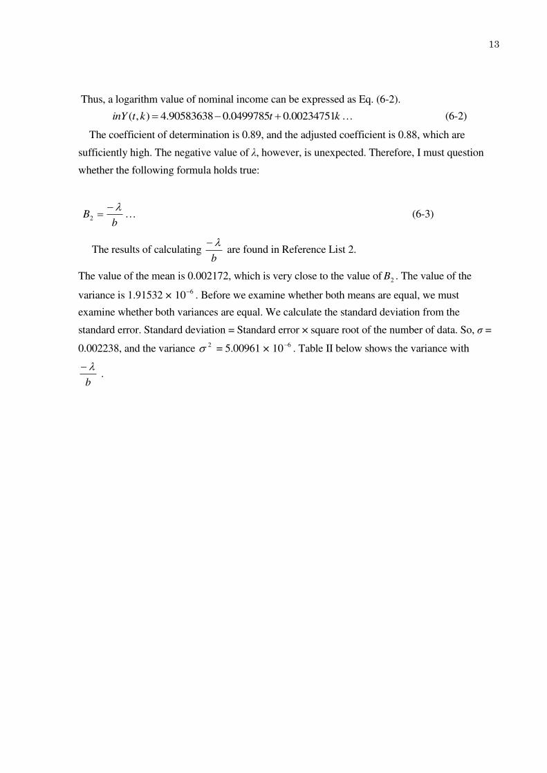
Thus, a logarithm value of nominal income can be expressed as Eq. (6-2).

ktktinY 00234751.00499785.090583638.4),( … (6-2)

The coefficient of determination is 0.89, and the adjusted coefficient is 0.88, which are

sufficiently high. The negative value of λ, however, is unexpected. Therefore, I must question

whether the following formula holds true:

b

B

2 … (6-3)

The results of calculating b

are found in Reference List 2.

The value of the mean is 0.002172, which is very close to the value of 2B . The value of the

variance is 1.91532 × 610 . Before we examine whether both means are equal, we must

examine whether both variances are equal. We calculate the standard deviation from the

standard error. Standard deviation = Standard error × square root of the number of data. So, σ =

0.002238, and the variance 2 = 5.00961 × 610 . Table II below shows the variance with

b

.

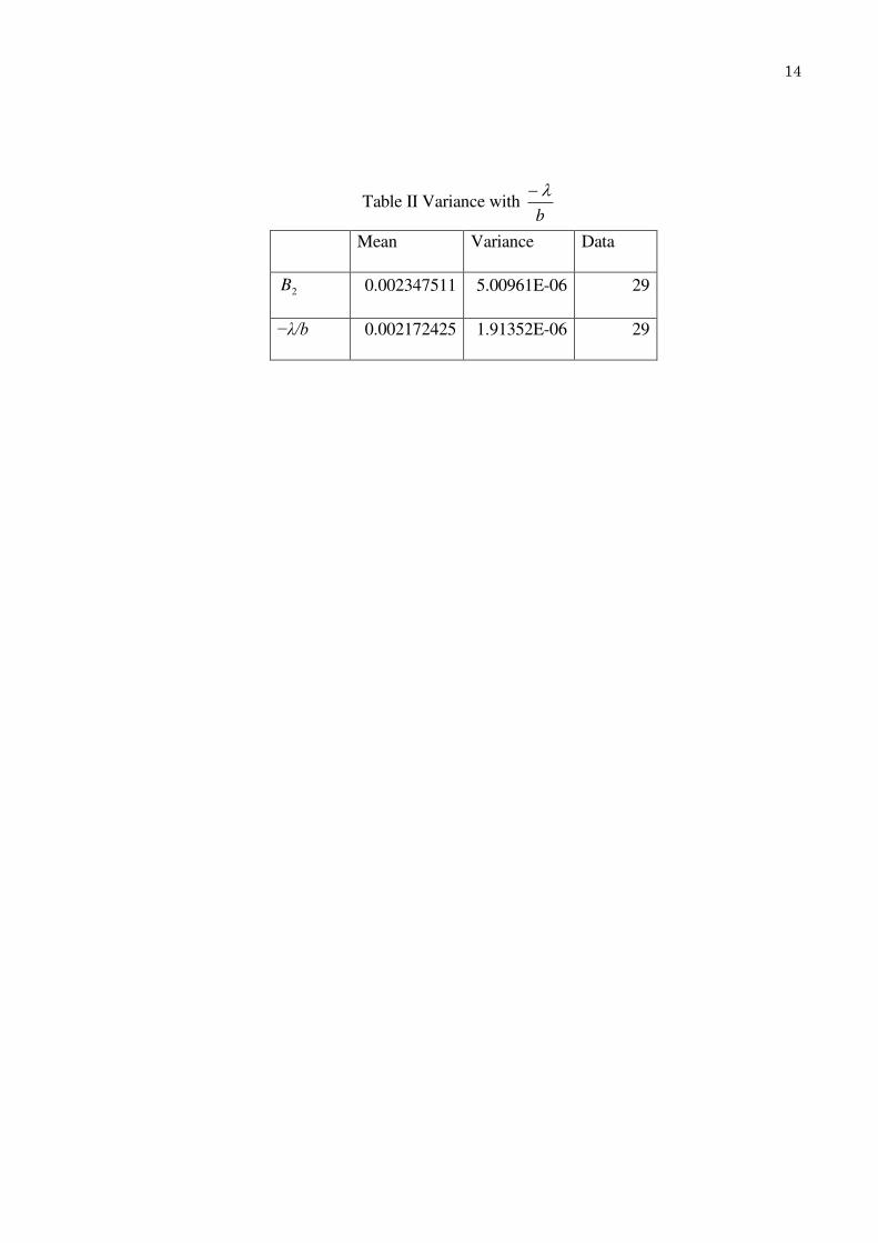
14

Table II Variance with b

Mean Variance Data

2B 0.002347511 5.00961E-06 29

−λ/b 0.002172425 1.91352E-06 29

15

We must seek the z value to examine whether both variances are equal. The z value is giveb

below.

2

2)1(

sn

z

in which n is a number of data, 2s is variance of

b

, and 2 is the variance of 2B .

That Z value has a chi-square distribution with n-1 degrees of freedom.

The answer is as follows:

z = 10.6951.

Rejection region of 0.005 left side: z 12.46134.

Rejection region of 0.005 right side: z 50.99338.

Thus, we can reject the hypothesis that the values of variances are equivalent with a 1% hazard

ratio.

To test the mean value between sets in which each has different variances, we use the

fact that t has a Student’s t-distribution with degrees of freedom.

The value of t is given below.

2

2

2

1

2

1

2

(nn

Bbt

Here, b

is the mean of

b

, 2

1 and 2

2 are variances, and 1n and 2n are numbers of the data

of b

and 2B , respectively.

The value of is given below.

1

)(

1

)(

)(

2

2

2

2

2

1

2

1

2

1

2

2

2

2

1

2

1

n

n

n

n

nn

16

The answers are below.

T = 0.358342321

= 47

Rejection region of 1% on both sides: 945630052.2t .

Thus, we cannot reject the hypothesis that both means are equivalent.

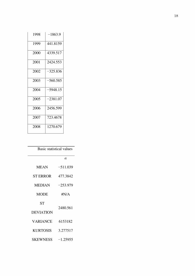
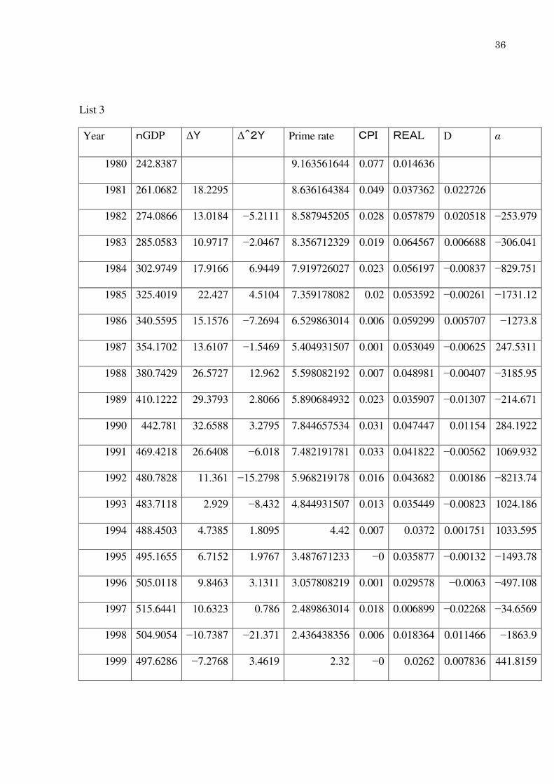
Next, we calculate the actual value of α. Reference List 3 shows the process of the

calculation. The results follow below.

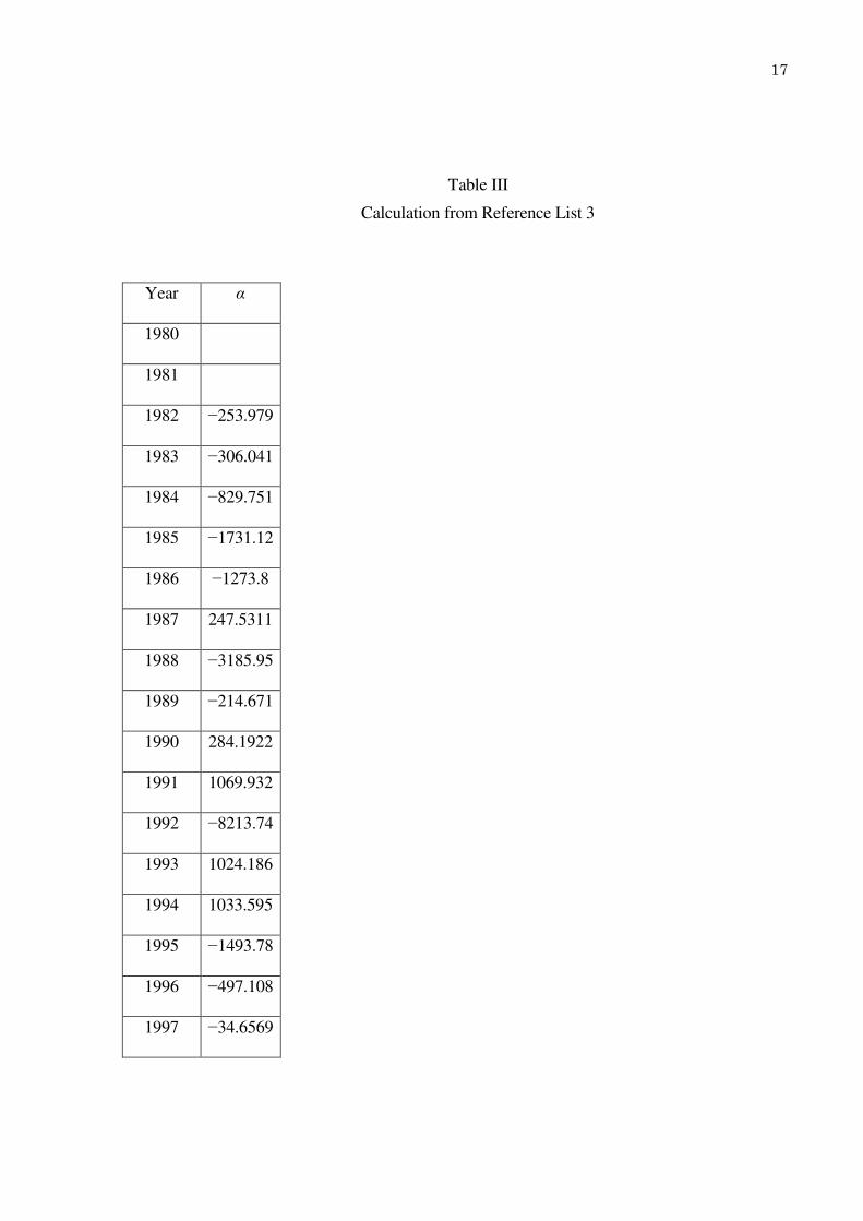
17

Table III

Calculation from Reference List 3

Year α

1980

1981

1982 −253.979

1983 −306.041

1984 −829.751

1985 −1731.12

1986 −1273.8

1987 247.5311

1988 −3185.95

1989 −214.671

1990 284.1922

1991 1069.932

1992 −8213.74

1993 1024.186

1994 1033.595

1995 −1493.78

1996 −497.108

1997 −34.6569

18

1998 −1863.9

1999 441.8159

2000 4339.517

2001 2424.553

2002 −325.836

2003 −560.585

2004 −5948.15

2005 −2381.07

2006 2456.599

2007 723.4678

2008 1270.679

Basic statistical values

α

MEAN −511.039

ST ERROR 477.3842

MEDIAN −253.979

MODE #N/A

ST

DEVIATION

2480.561

VARIANCE 6153182

KURTOSIS 3.277517

SKEWNESS −1.25955

19

RANGE 12553.25

MIN −8213.74

MAX 4339.517

TOTAL −13798.1

DATA 27

C-INTER

(95.0%)

981.2772

20

The mean of α is －511 (trillion yen）２

, which is very close to the actual GDP. Hence, α must

be negative to maintain stable growth because λ is negative.

The standard deviation (ST DEVIATION) is 2480.561 (trillion yen),which is quite large.

Its value divided by 10 trillion is very close tob

.

The skewness is negative. The mass of the distribution is concentrated on the right side

of the figure. We find a consecutive series of negative figures from 1982 to 1989 and from

2002 to 2005. We conduct a regression analysis by selecting only the years having negative α.

Then we examine whether the capability of this model becomes stronger. The following are the

results:

The coefficient of determination increases to 0.93 from 0.89.

The one adjusted by degree of freedom grows to 0.92 from 0.88. We can confirm that

this model is best applied to a condition with negative α.

Coefficient of determination: 0.934773.

Coefficient of determination adjusted by degree of freedom: 0.924738.

21

Table IV Results of analysis ②

Coefficient

Standard

deviation

t P-Value

0B 4.909718 0.1489163 32.96964 6.46E-14

1B −0.05517 0.0158882 −3.47251 0.004126

2B 0.002447 0.0004736 5.166249 0.000181

22

Next, we verify that (4-19) can be reliably applied to an actual case. Eq. (4-19)

calculates real income based on the assumption that real income is the equilibrium income on

the condition that α = 0. I confirmed that this income is the real GDP, ),(*ktY .

)exp()(),( 21

*k

btkCCktY

… (4-19)

Then ｋ）ＣｋＣ

ｋＣ＝（ ２

２

2１21

CkCC

.

If we define ｋＣ

ｋ＋ＣＣ＝Ｃ

２

２１３ ,

ｋＣ ２321 CkCC .

So we rewrite λ as 1 in (4-19）

Thus, (4-19) becomes (6-4).

)exp()(),( 11

2

23

*k

btkCCktY

… (6-4)

We assume real income is expressed as a well-known function, as in (6-5) below, whose

capital elasticity of income is a.

aAkkY )(* … (6-5) (A: constant)

Hence, we can expect that 2

2C is the following function:

inka

kCC

2

4

2

2 )(exp … (6-6)

kb

1

We insert that function into (6-4).

))(exp(exp),( 1143

*k

btkCCktY ink

a

)2

exp(),( 1143

*k

btkCCktY ink

a

… (6-5)

Putting both sides into the logarithm, we get:

kb

tinkinCinCktinY inka

1143

* 2),(

… (6-6)

23

We differentiate both sides with respect to t.

bbk

dtdk

aY

dtdY

11*

*

2

bb

bbk

dtdk

aY

dtdY

11

1

*

*

2

k

dtdk

aY

dtdY

*

*

So we confirm that a is the capital elasticity of income.

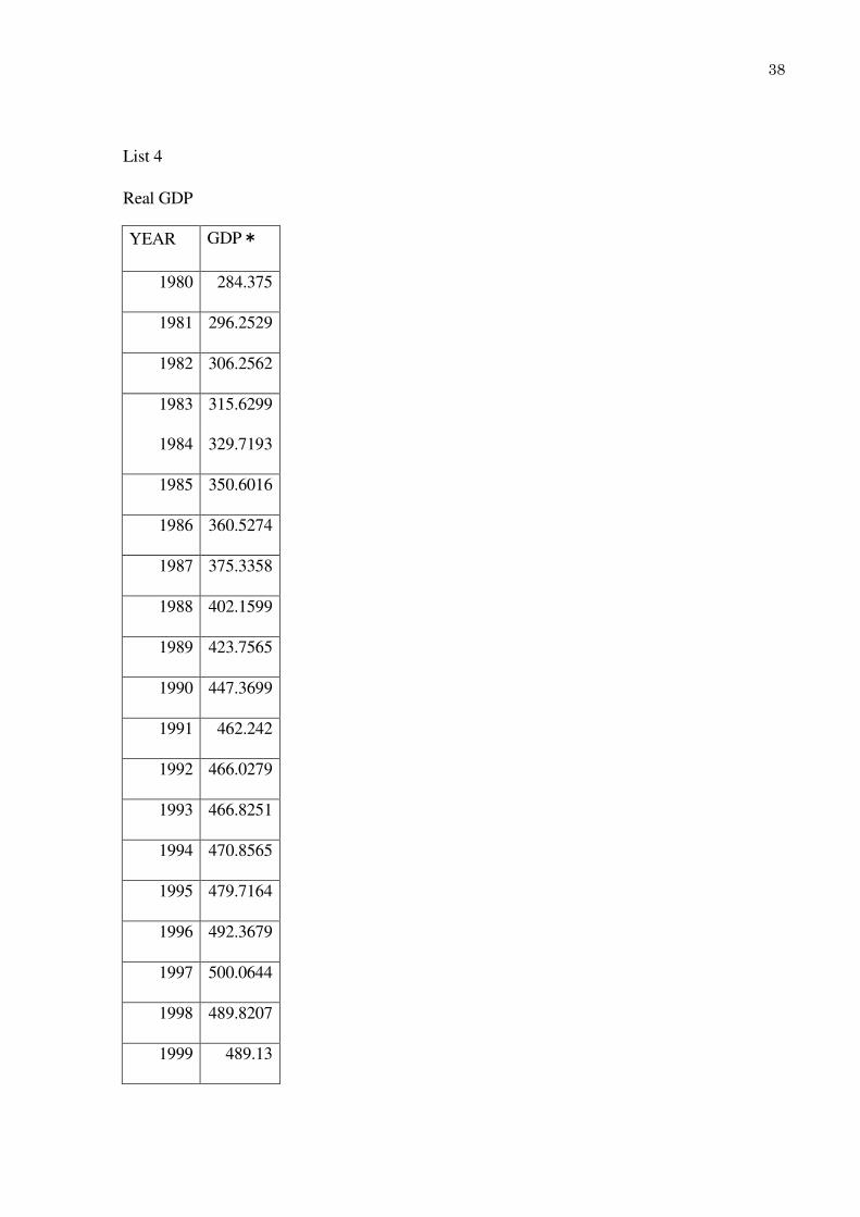
Additionally, (6-6) shows that *inY can be brought into the regression analysis with

respect to ink , t, and k. Therefore, we use the data of real GDP from Reference List 4, with the

results that

Coefficient of determination: 0.989992444.

Adjusted Coefficient of determination by degrees of freedom: 0.9887415.

24

Table V Results of Analysis ③

Coefficient St Error t P-value

0B −0.515 14704 0.480274 −1.0726 0.2941

1B 1.119219197 0.090926 12.3091 7E-12

2B 0.014294401 0.004325 3.30509 0.003

3B −0.00128167 0.000226 −5.6828 7E-06

25

That is, the logarithm of real income can be expressed as the following function:

ktinkktinY 00128167.0014294401.0119219197.1515154704.0),(* … (6-7)

The coefficient of determination is 0.98, as is the adjusted coefficient. Thus, we can confirm the

model works remarkably well.

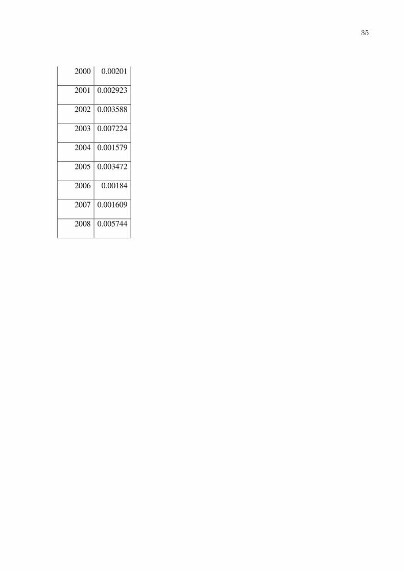
Reference List 5 shows that b

12s. The value of the mean is

00117895.02 1

b

This is very close to 3B . We test these values as we did earlier.

26

Table VI Variance with b

12

MEAN VARIANCE DATA

B3 −0.001282 1.4243E-06 28

b12

-0.001179 5.0555E-07 27

27

First, we examine whether the variances are equal.

We calculate the Z value as before: 2287136.9Z .

Rejection region of 0.005 left side: 167237.11Z .

Therefore, we can reject the hypothesis that the values of variances are equivalent.

Then we calculate the t value and degrees of freedom as before:

3893929.0t

44

Rejection region of 1% both sides: 995534.2t

Therefore, we cannot reject the hypothesis that both means are equivalent.

7. Implications for Financial Policy

For policymakers, the equation implies that the economy would not ascend on a stable

course if the product of α and λ is not positive. To maintain economic stability when λ is

positive, α should be positive; however, when λ is negative, α should be negative. To sustain a

positive value for α, policymakers must increase the interest rate whenever income accelerates

and reduce it whenever income decelerates. Yet, to sustain a negative value for α, they must

decrease the interest rate when income accelerates and increase the interest rate when income

decelerates. In Japan’s case, λ is negative, so α should be negative.

Policy may be able to reduce the interest rate whenever there is acceleration, but it may

seem impossible to increase the interest rate during deceleration. However, we may have an

available strategy for such a policy. First, we assume that the current real growth rate is the

equilibrium growth rate. Then, we decrease the interest rate and increase the real growth rate to

be more than the equilibrium growth rate, followed by gradually raising the interest rate. We

must continue to increase the interest rate until the real growth rate is equal to a new

equilibrium growth rate. By this logic, we must quickly attempt to increase the interest rate

when the real growth rate exceeds the current equilibrium growth rate.

If the economy shifts to a higher equilibrium as it continues to grow, the economy

accelerates further. If so, when the economy reaches the new equilibrium, we will see the

higher interest rate. Then we can decrease that interest rate to re-stimulate the economy. Thus,

the interest rate will increase as the equilibrium growth rate rises.

We may increase much supply compared to demand on the condition that λ is negative.

28

If we stimulate the economy by reducing the interest indiscreetly while maintaining a

stable equilibrium growth rate, we will see smaller rates of both interest and growth. Currently,

Japan’s real growth rate is approximately 1% and its interest rate is approximately 1.5%. Both

may have reached their lower limits. Japan must soon seek an economic strategy for raising the

equilibrium growth rate.

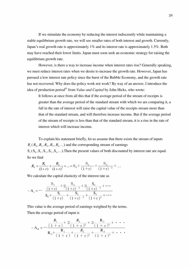
However, is there a way to increase income when interest rates rise? Generally speaking,

we must reduce interest rates when we desire to increase the growth rate. However, Japan has

pursued a low interest rate policy since the burst of the Bubble Economy, and the growth rate

has not recovered. Why does the policy work not work? By way of an answer, I introduce the

idea of production periodiii

from Value and Capital by John Hicks, who wrote:

It follows at once from all this that if the average period of the stream of receipts is

greater than the average period of the standard stream with which we are comparing it, a

fall in the rate of interest will raise the capital value of the receipts stream more than

that of the standard stream, and will therefore increase income. But if the average period

of the stream of receipts is less than that of the standard stream, it is a rise in the rate of

interest which will increase income.

To explain his statement briefly, let us assume that there exists the stream of inputs

tR ( 0R , 1R , 2R , 3R , 4R …) and the corresponding stream of earnings

ｔS ( 0S , 1S , 2S , 3S , 4S …).Then the present values of both discounted by interest rate are equal.

So we find

＋（１＋ｒ）

Ｓ＋

（１＋ｒ）

Ｓ＋Ｓ...

)1()1( ２

２1０2

21０

r

R

r

RR …

We calculate the capital elasticity of the interest rate as

＋・・・（１＋ｒ

S＋

（１＋ｒ）

S＋

（１＋ｒ）

S＋S

＋・・・（１＋ｒ）

S＋３

（１＋ｒ）

Ｓ＋２

（１＋ｒ）

Ｓ

ー

３３

２２１

０

３３

２２１

)

s

This value is the average period of earnings weighted by the terms.

Then the average period of input is

＋・・・（１＋ｒ）＋

（１＋ｒ）＋

（１＋ｒ）＋

＋・・・（１＋ｒ）

＋３（１＋ｒ）

＋２（１＋ｒ）ー

３

３

２

２１０

３

３

２

２１

RRR

R

R

RR

R

29

Then, if Rs , a decline in interest rates causes income to increase, and if Rs , an

increase in the interest rate leads to an increase in income.

Now we calculate the average period when inputs or earnings are constant.

If

4310 RRRR …

or

S S S S S ４３２１０ …

So the average period of inputs or earnings resembles the following equation:

r

r

r

rr

r 1

)1(

11

)1(

1

))1(

11(

1

))1(

11(

)1(

1

1111

111

2

＋（１＋ｒ）＋

（１＋ｒ）＋

（１＋ｒ）＋

＋（１＋ｒ）

＋３（１＋ｒ）

＋２（１＋ｒ）

３２

３２

That is equal to the reciprocal of the interest rate. If the stream has a crescendo, the average

period of the stream is longer than the reciprocal of interest rate. If the stream has a decrescendo,

its average period is shorter than the reciprocal of the interest rate. I think that the average

period of inputs generally extends as the economy progresses, but that of earnings becomes

longer; therefore, a fall in the interest rate causes an increase in income.

However, if we assume the stream of inputs is constant, then an average period of

inputs is equal to the reciprocal of interest rate, and it is shorter than the average period of

earnings. Then we find the equation

Rs

In that case, in general, the interest rate should rise to increase income. We must pay attention

not to the absolute level of interest rate, but rather, to the magnitude of the relation between

average periods of inputs and earnings.

If the interest rate is 1.5%, the reciprocal is approximately 67 years. So to reduce

interest rates further is unproductive if the stream of inputs is constant and the average period of

earnings is less than 67 years. As Hicks demonstrated, one cannot expect income to increase by

decreasing interest rates indiscreetly.

8. Conclusion

Nominal GDP can be expressed as the equation

If 0

30

)exp(),( 1 kb

tCktY

… （4-16）

or

)exp(),( 1 kb

tCktY

… （4-17)

If 0

))(2

sin())(2

cos()()(2

)2(exp(),( 321 k

bbCk

bbCk

bb

btPktY

… （4-20）

If (4-16) can be applied, real income can be expressed as (6-8)

)2

exp(),( 1

43

*k

btkCCktY ink

a

… (6-8）

kb

12

(a: income elasticity of capital)

Statistical research shows Japan’s GDP can be expressed by the following equations:

Nominal income Y

ktktinY 00234751.00499785.090583638.4),( … (6-2）

Real income *

Y

ktinkktinY 00128167.0014294401.0119219197.1515154704.0),( …（6-10）

From Section 4, we can show that a sign of αλ determines which type of equation can be

applied:

If αλ > 0: (4-16) or (4-17）

If αλ < 0: (4-20）

The solution to this equation may provide a firm underpinning to economic policy by

the following logic. Assuming that the trend of time is positive (λ > 0), policymakers must

increase the interest rate whenever economic growth accelerates, and decrease it when growth

decelerates. This action can lead the economy to a stable course because it preserves the

condition that α > 0, as shown by (4-16) or (4-17). In other words, we must increase the interest

rate rather than decrease it to keep acceleration positive whenever the real growth rate is lesser

than the equilibrium growth rate.

However, if λ < 0, the recommendation is reversed. We must decrease the interest rate

whenever the economy accelerates and increase it in the event of deceleration. Thus, since

Japan has negative λ, we may be able to decrease the interest rate whenever there is acceleration,

but it may seem impossible to increase the interest rate in the event of deceleration.

31

Nonetheless, we may have a strategy available for such a policy. First, we assume the

current real growth rate is the equilibrium growth rate. Then, we decrease the interest rate and

increase the real growth rate making it more than the equilibrium growth rate, followed by

gradually increasing the interest rate. We must continue to increase the interest rate until the

real growth rate is equal to a new equilibrium growth rate. By this logic, we must quickly

attempt to increase the interest rate when the real growth rate becomes higher than the current

equilibrium growth rate.

If the economy shifts to a higher equilibrium as it continues to grow, the economy will

accelerate further. If so, when the economy reaches the new equilibrium, we will see higher

interest rates. Then we can reduce that interest rate to re-stimulate the economy. Thus, the

interest rate will increase as the equilibrium growth rate rises.

We may increase much supply compared to demand on the condition that λ is negative.

However, our condition that both λ and α are negative to maintain economic stability can

be considered a shrinking economy. If we stimulate the economy by reducing the interest rate

indiscreetly while maintaining a stable equilibrium growth rate, we will achieve smaller rates of

both interest and growth. Currently, Japan’s real growth rate is approximately 1% and its

interest rate is approximately 1.2%. Both may have reached their lower limits. Japan’s policymakers must soon seek an economic strategy for raising the equilibrium growth rate.

It is difficult to change basic beliefs about financial policy. But if policymakers hope to

effect real-world change, they first must change their economic thought. John Maynard Keynes

long ago noted the stubbornness of economic thought:

But besides this contemporary mood, the ideas of economists and political philosophers,

both when they are right and when they are wrong, are more powerful than is

commonly understood. Indeed the world is ruled by little else. Practical men, who

believe themselves to be quite exempt from any intellectual influences, are usually the

slaves of some defunct economist.

Japan has imposed a low interest rate policy for many years, and the result has been persistent

deflation. If we maintain a low interest rate policy and do not fully consider the alternative

presented in this research, we are acting unreasonably. Now is the time to try new theories and

new economic thoughts.

9．References

List 1

32

Year

GDP

（Nominal）

Capital

Stock

（Begin）

1980 242.8387 358.4012

1981 261.0682 382.292

1982 274.0866 405.8706

1983 285.0583 427.7703

1984 302.9749 447.2519

1985 325.4019 471.3132

1986 340.5595 524.3229

1987 354.1702 554.6213

1988 380.7429 595.5875

1989 410.1222 632.2497

1990 442.781 677.281

1991 469.4218 726.7462

1992 480.7828 786.1105

1993 483.7118 826.5722

1994 488.4503 857.0921

1995 495.1655 888.7079

1996 505.0118 918.2468

1997 515.6441 948.9018

1998 504.9054 980.756

1999 497.6286 1005.381

33

2000 502.9899 1026.533

2001 497.7197 1051.391

2002 491.3122 1068.489

2003 490.294 1082.417

2004 498.3284 1089.336

2005 501.7344 1120.987

2006 507.3648 1135.384

2007 515.5204 1162.551

2008 505.1119 1193.615

¥ Trillion

34

List 2

YEAR −λ／ｂ

1980 0.002092

1981 0.00212

1982 0.002282

1983 0.002565

1984 0.002077

1985 0.000943

1986 0.00165

1987 0.00122

1988 0.001363

1989 0.00111

1990 0.00101

1991 0.000842

1992 0.001235

1993 0.001638

1994 0.001581

1995 0.001692

1996 0.00163

1997 0.001569

1998 0.00203

1999 0.002363

35

2000 0.00201

2001 0.002923

2002 0.003588

2003 0.007224

2004 0.001579

2005 0.003472

2006 0.00184

2007 0.001609

2008 0.005744

36

List 3

Year ｎGDP ΔＹ Δ＾２Ｙ Prime rate ＣＰＩ ＲＥＡL D α

1980 242.8387 9.163561644 0.077 0.014636

1981 261.0682 18.2295 8.636164384 0.049 0.037362 0.022726

1982 274.0866 13.0184 −5.2111 8.587945205 0.028 0.057879 0.020518 −253.979

1983 285.0583 10.9717 −2.0467 8.356712329 0.019 0.064567 0.006688 −306.041

1984 302.9749 17.9166 6.9449 7.919726027 0.023 0.056197 −0.00837 −829.751

1985 325.4019 22.427 4.5104 7.359178082 0.02 0.053592 −0.00261 −1731.12

1986 340.5595 15.1576 −7.2694 6.529863014 0.006 0.059299 0.005707 −1273.8

1987 354.1702 13.6107 −1.5469 5.404931507 0.001 0.053049 −0.00625 247.5311

1988 380.7429 26.5727 12.962 5.598082192 0.007 0.048981 −0.00407 −3185.95

1989 410.1222 29.3793 2.8066 5.890684932 0.023 0.035907 −0.01307 −214.671

1990 442.781 32.6588 3.2795 7.844657534 0.031 0.047447 0.01154 284.1922

1991 469.4218 26.6408 −6.018 7.482191781 0.033 0.041822 −0.00562 1069.932

1992 480.7828 11.361 −15.2798 5.968219178 0.016 0.043682 0.00186 −8213.74

1993 483.7118 2.929 −8.432 4.844931507 0.013 0.035449 −0.00823 1024.186

1994 488.4503 4.7385 1.8095 4.42 0.007 0.0372 0.001751 1033.595

1995 495.1655 6.7152 1.9767 3.487671233 −0 0.035877 −0.00132 −1493.78

1996 505.0118 9.8463 3.1311 3.057808219 0.001 0.029578 −0.0063 −497.108

1997 515.6441 10.6323 0.786 2.489863014 0.018 0.006899 −0.02268 −34.6569

1998 504.9054 −10.7387 −21.371 2.436438356 0.006 0.018364 0.011466 −1863.9

1999 497.6286 −7.2768 3.4619 2.32 −0 0.0262 0.007836 441.8159

37

2000 502.9899 5.3613 12.6381 2.211232877 −0.01 0.029112 0.002912 4339.517

2001 497.7197 −5.2702 −10.6315 1.772739726 −0.01 0.024727 −0.00438 2424.553

2002 491.3122 −6.4075 −1.1373 1.921780822 −0.01 0.028218 0.00349 −325.836

2003 490.294 −1.0182 5.3893 1.560410959 −0 0.018604 −0.00961 −560.585

2004 498.3284 8.0344 9.0526 1.708219178 0 0.017082 −0.00152 −5948.15

2005 501.7344 3.406 −4.6284 1.60260274 −0 0.019026 0.001944 −2381.07

2006 507.3648 5.6304 2.2244 2.293150685 0.003 0.019932 0.000905 2456.599

2007 515.5204 8.1556 2.5252 2.342191781 0 0.023422 0.00349 723.4678

2008 505.1119 −10.4085 −18.5641 2.281232877 0.014 0.008812 −0.01461 1270.679

＊1 Prime rates weighted averages by term

＊2 CPI stands for consumer price index

＊3 Real is the real interest rate, that is, the difference between CPI and the prime rate

＊4 D is the difference in real interest rates

38

List 4

Real GDP

YEAR GDP＊

1980 284.375

1981 296.2529

1982 306.2562

1983 315.6299

1984 329.7193

1985 350.6016

1986 360.5274

1987 375.3358

1988 402.1599

1989 423.7565

1990 447.3699

1991 462.242

1992 466.0279

1993 466.8251

1994 470.8565

1995 479.7164

1996 492.3679

1997 500.0644

1998 489.8207

1999 489.13

39

2000 503.1198

2001 504.0475

2002 505.3694

2003 512.513

2004 526.5777

2005 536.7622

2006 547.7093

2007 560.8164

¥ Trillion

40

List 5

YEAR b

12

1980

1981 −0.0012

1982 −0.00121

1983 −0.00131

1984 −0.00147

1985 −0.00119

1986 −0.00054

1987 −0.00094

1988 −0.0007

1989 −0.00078

1990 −0.00063

1991 −0.00058

1992 −0.00048

1993 −0.00071

1994 −0.00094

1995 −0.0009

1996 −0.00097

1997 −0.00093

1998 −0.0009

1999 −0.00116

41

2000 −0.00135

2001 −0.00115

2002 −0.00167

2003 −0.00205

2004 −0.00413

2005 −0.0009

2006 −0.00199

2007 −0.00105

42

〔1〕 Ryou Kato, Modern Macro Economic Lecture, 53-57, Toyo Keizai Inc 2007.

〔2〕Nobutyuki Oda and Murakami Jun, Natural Interest Rate, 11-14 Bank of Japan

Working Paper Series No－J―5.

〔3〕John Hicks, Value and Capital, 171-188, Oxford At The Clarendon Press. 1939.