A Passage to India:

Quantifying Internal and External Barriers to Trade

Eva Van Leemput*

Department of Economics

University of Notre Dame

Abstract

This paper quantifies the size of intra-country versus inter-country trade barriers and assesses

the impact on patterns of trade and welfare. I develop a quantitative multi-sector international

trade model featuring non-homothetic preferences in which states trade both within country

and internationally. I discipline the model using rich micro data on foreign and domestic trade

flows at the Indian state level and price dispersion both within and across states. I find that: (1)

state-wise price data predict internal trade flows well; (2) internal trade barriers make up 30%

of the total trade cost on average, but vary substantially by state depending on the distance to

the closest port; and (3) the welfare impacts of domestic integration are substantial; reducing

trade costs across states to the U.S. level increases welfare by 15% compared to a welfare gain

of 7% when fully eliminating international import barriers.

JEL Classification: F1, O1.

Key Words: Internal Trade, International Trade, Welfare

*Contact information: evanleem@nd.edu, (574) 904-4430, Notre Dame, IN 46556. I thank my advisor JosephKaboski, my committee members Nelson Mark, Wyatt Brooks and Kevin Donovan, and helpful comments fromseminar participants at Notre Dame, XIX Workshop on Dynamic Macroeconomics, the IMF, and the Federal ReserveBank of Chicago.

1 Introduction

International barriers to trade, and the benefits from reducing them, have been a focus of policy

and research for decades, but recently policy has focused more on internal trade barriers and their

role in improving the economy. For example, in 2014, the World Bank Group announced that

its financing commitments in roads, bridges, energy, clean water, and other critical infrastructure

projects increased by 45% to $24 billion compared to 2013. Although these projects are intended

to increase regional integration, they also have an impact on international trade. When countries

have large populations that are separated from a main port or border, imported goods not only

have to reach the port, but must also reach rural and/or landlocked urban areas. This can increase

the cost of imports tremendously, especially when domestic trade frictions are high. In fact, recent

micro-founded studies have found that these intra-country trade costs are substantially higher for

developing countries, making trade very costly.

This paper quantitatively addresses two main questions: (1) How large are within country trade

barriers versus international trade barriers?, and (2) What are the welfare implications of regional

integration compared to international integration? Whereas the literature has mostly focused on

estimating either the impact of improved regional integration or increased international integration,

the main contribution of this paper is to first quantify the barriers to internal and international trade

and then compare the welfare implications of relaxing those barriers. Moreover, this setting allows

for different types of regional integration: rural-urban integration and connecting states within a

country. Finally, this paper will disentangle the size of the main barriers to foreign markets access:

border costs the port versus domestic frictions to reach ports in landlocked states.

I find that, on average, total internal trade frictions, which include both the within- and across-

state trade costs, make up 30% of the total trade cost, but vary substantially by state, depending on

the distance to the closest port. Secondly, there are large welfare gains from state-wise integration.

Reducing trade costs across states to the U.S. level increases welfare by 15% compared to a welfare

gain of 7% when fully eliminating international import barriers. Finally, by decomposing internal

trade barriers, I find that eliminating rural-urban trade costs increases welfare by 5%. This suggests

that the largest barrier within India is not the rural-urban trade barrier, but is driven by Indian

states not being well connected.

1

I develop a quantitative international trade model that explicitly accounts for internal trade

frictions. Indian states trade both with other states and with the rest of the world. Consumers

have non-homothetic preferences over agricultural and manufacturing goods. Each state consists

of a rural and an urban region, which produces agricultural and manufacturing goods, respectively.

I model three types of trade costs. Trade between urban and rural areas is costly, even within the

same state. Trade across states entails an additional cost. Hence, domestic trade frictions in India

comprise of an urban-rural trade cost within state and an inter-state trade cost. Finally, if states

trade internationally, they face the standard international trade costs. Not every state has its own

international port in their state, and all international trade must flow through international ports.

Hence, landlocked states face additional, within-country, costs of importing and exporting.

In order to map the model to the Indian economy, I combine three rich micro level data sets.

Together, the State Movement/Flows of Goods data and the Foreign Trade Statistics for India

detail good-specific trade flows both bilaterally across Indian states and state-specific imports and

exports. On the export side, it includes the state of origin and destination for inter-state trade

and includes the port of exit for international trade. For imports, it includes the state of origin

in the case of inter-state trade and the port via which international trade occurs. Thus, I can

distinguish, for example, between inter-state flows that are ultimately destined for the state, and

those that are ultimately destined for international trade. This allows for a precise delineation

of border costs and domestic trade barriers. Lastly, to discipline the trade costs both within and

across states, I use data containing measures of price dispersion of wholesale agricultural prices,

published by the Data Portal India. This data set consists of state-, market-, and variety-specific

wholesale prices of 110 different agricultural goods across 1850 markets in all Indian states. Using

an no-arbitrage argument, I compute cross-state trade barriers, and I find these are six times larger

than the U.S., which is around the same magnitude as other micro evidence has estimated.1 To

discipline the rural-urban trade costs, I use the same methodology using the price variation across

markets within state. I find trade costs comparable to half of inter-state costs in the U.S. Finally, I

compute international trade costs by matching state-wise international trade flows for agriculture

and manufacturing.

1The inter-state barriers in the U.S. are computed across all 50 states and the District of Columbia using state-wiseUSDA prices.

2

I use state-wise price dispersion for agricultural goods to estimate the trade elasticity for agri-

culture following the methods outlined in Simonovska and Waugh (2014). I find the elasticity to be

almost as large as the one the trade literature has estimated for manufacturing, suggestive of large

gains from trade, even across Indian states. Finally, I use detailed state-specific data in India to

identify some of the other main parameters in the model. The Ministry of Statistics and Program

Implementation provides data on state-wise total population of which the percentage urban and

rural. This pins down the population in each region in each state in the model. Value added per

capita for agriculture and manufacturing serves as proxy for sectoral wages as is standard in the

literature. I find that, on average, wages in the urban areas are three times larger as in the rural

areas which is consistent with Restuccia et al. (2008).

Using price dispersion to discipline trade barriers has several advantages over direct measures of

trade costs. As the focus of this paper is not the nature of trade barriers, using price dispersion is

preferred since it encompasses more than just infrastructure barriers. I show that price dispersion

both across and within states predict internal trade flows well and outperform measures of distance.

Secondly, I provide evidence that accounting for differential port access is quantitatively important

in terms of explaining international trade flows. Again, using the price variation provides a better

fit than regular distance measures. For instance, I find that inter-state trade barriers for Jharkand

are relatively high using price dispersion measures, although they are close to a major port state,

West Bengal. And in fact, they trade less internationally than Bihar, a state that is further removed

from West Bengal.

The remainder of the paper is organized as follows. The next section describes the related

literature to which this paper contributes. Section 2 presents the motivating empirical facts that

motivate the theory. Section outlines the international trade model. Section 4 describes the data

used in the analysis and the calibration of the model and section 5 presents the results. Section 6

concludes.

Related Literature

This paper builds on the seminal model of geography and trade of Eaton and Kortum (2002) and

on Fieler (2011)’s two sector extension, and it contributes to two main literatures. The first is

examining the size, nature and impact of international trade cost in explaining international trade

3

patterns. Waugh (2010) studies the size of trade barriers across developed and developing countries

countries. He finds that trade frictions between rich and poor countries are systematically asym-

metric, with poor countries facing higher costs to export relative to rich countries. Tombe (2014)

also estimates larger trade costs for developing countries, but argues that these countries especially

face large trade costs in agriculture. In terms of the components of international trade barriers,

Limao and Venables (1999) find that infrastructure is an important determinant of transport costs,

especially for landlocked countries. They estimate that halving transport costs would increase trade

volume by a factor of five. In more recent work, Hummels and Schaur (2013) estimate that time

in transit poses a large international trade barrier. In fact, they find that each day in transit is

equivalent to an ad-valorem tariff of 0.6 to 2.3 percent. The focus of all the papers in this literature

is on border costs. My paper complements these works by disentangling border costs from within

country costs, and assess their respective impact on trade.

Second, I contribute to an emerging literature examining the role of intra-national trade costs

on the production and trade patterns in developing countries. Based on detailed micro-data,

Donaldson (2014), Atkin and Donaldson (2014), Allen (2014), Asturias et al. (2014), Adamopoulos

(2011) quantify the size and nature of intra-country trade frictions within developing countries but

do not compare these costs to international trade barriers.2 Other recent work has estimated the

effects of regions with differential market access within countries on the gains from trade: Behrens

et al. (2006) find that for regions that are “geographically disadvantaged” with high intra-country

trade costs, being remote acts as a barrier to competition from abroad. Storeygard (2014) shows

that regions in sub-Saharan Africa with better access to port cities benefit more from terms of trade

shocks. Cocar and Fajgelbaum (2014) develop a framework for the spatial distribution of economic

activity in an arbitrary topography of trade costs where products are differentiated by origin. They

find that in the presence of high domestic frictions, international trade creates a partition between

a commercially integrated coastal region with high population density and an interior region where

immobile factors are poorer. Gollin and Rogerson (2014) examine the interaction of intra-country

trade patterns on employment patterns between agricultural and manufacturing sectors taken as

given that developing countries import very little agriculture. My paper shows the impact of these

2For instance, Atkin and Donaldson (2014) find infrastructure costs being 7-15 times higher in Ethiopia thansimilar estimates for the U.S.

4

within country trade frictions on international trade patterns. The distinctive aspect in this paper is

the state-wise regional and international trade data and the state-wise characteristics in each state.

Previous studies have differentiated within country trade flows, but only aggregate international

trade flows. In this paper, I can distinguish international trade by state and also via which ports

trade happens. As I will show, this is quantitatively important in explaining aggregate trade flows

and matters for the impact of international trade policies in terms of heterogeneity across states.

Moreover, this framework allows to compare regional versus international integration and its welfare

implication. In other words, “What are the gains to trade from India trading with the rest of the

world versus becoming more integrated itself?”.

2 Empirical Evidence

This section establishes the empirical facts that motivate the theory. First I show that develop-

ing countries trade very little internationally and especially agriculture. Second, I document the

existence of large price dispersion for agricultural goods in developing countries.

2.1 International Trade

Table 1 breaks down total international trade and expenditures by agriculture and manufacturing

for 2009. The import shares represent total international imports over domestic consumption which

is given by: ∑iXni,g

Xn,g=

∑iImportsni,g

GrossProductionn,g=Total Exportsn,g + Importsn,g

where Xni,g represent total imports from country i to country n for good type g: agriculture or

manufacturing. Clearly, India, Africa and South America import less overall compared to the U.S.

and Europe. However, more strikingly, developing countries are importing very little agriculture

as opposed to Europe and the U.S., although a large fraction of their expenditures is going to

agricultural products. In India for instance, international agricultural imports only represent 5%

of total food consumption whereas food expenditures make up 37%. By comparison, in the U.S.

33% of total food consumption is imported whereas total food expenditures make up 6%. This

shows that developing countries mostly consume domestically produced food and are less integrated

5

internationally as opposed developed countries. As mentioned earlier, most of the focus has been

on larger international border costs and have been estimated to be larger for developing countries.

Table 1: Breakdown International Trade Flows (2009)

Import Shares Consumption

Agriculture Manufacturing Agriculture Manufacturing

U.S. 33% 42% 6% 94%

Europe 57% 69% 9% 91%

Africa 4% 18% 45% 55%

South America 8% 21% 24% 76%

India 5% 11% 37% 63%

Source: UNIDO, UN Comtrade (2009)

2.2 Domestic Trade Barriers

Current research has explained these trade patterns by estimating large trade barriers for developing

countries and substantially higher trade costs for agricultural trade. However, this section will

show that developing countries exhibit substantial within country deviations from the Law-of-One-

Price, suggestive of large internal trade costs. To provide evidence that markets within developing

countries less integrated than developed countries, I use the concept of Law-of-One-Price (LOP)

within countries following Crucini and Shintani (2008). Define pjit the price for good j in market i

at time t. The good-level log law-of-one-price deviation measure qjit within a country:

qjit = ln pjit − ln pjt

where pjt is the mean price across markets within the same country. The first set of data is

reported by the USDA and the second set is taken from FAOSTAT and the UN world food program.

One issue that can arise when comparing good-specific prices across markets are differences in

quality. However, it is very unlikely that this is the main driving force since (1) the data are highly

disaggregated, for instance, white corn, and (2) the patterns hold across different commodities.

6

Figure 1 plots the distribution of Law-of-One-Price deviations of corn across different markets

within the US, India and two African countries: Malawi and Niger. The density is centered at zero,

by construction and estimated using a Gaussian kernel. If LOP held, the distribution would be

degenerate at zero. Clearly, LOP does not hold for all countries. However, prices are more dispersed

within India and African countries than within the U.S. This is suggestive of large domestic trade

frictions that impede price convergence across market in developing countries. The contribution of

this paper is to quantify how large these domestic frictions are as opposed to international trade

frictions and the impact on trade patterns and welfare of relaxing these trade barriers.

Figure 1: Law-of-One-Price Deviation Density within Country (2012)

Source: USDA, AGMARKNET, FAOSTAT (2012)

3 Model

The model extends the Eaton-Kortum (2002) framework to include many states within a country

that consist of both rural and urban regions. More concretely, I model trade between a large multi-

state country and a second uniform country representing the rest of the world. The quantitative

analysis is based on the Indian economy and therefore, the model is presented accordingly.

7

3.1 Environment

India consists of multiple states denoted by s = 1, ..., S. Each state consists of two regions: a rural

and urban area indexed by r = {R,U}. This economy produces two types of goods: agriculture and

manufacturing, indexed by g ∈ {a,m} where a denotes agricultural goods and m manufacturing

goods. For each good, there is a continuum of individual varieties jg defined on the interval

[0, 1]. All agricultural production takes place in the rural area and the urban region produces all

manufacturing goods.3 Both good types are produced with Ricardian technology and require only

labor for production which is immobile across regions and states. More specifically, I assume that

the share of workers in the rural area is βs ∈ [0, 1] and and at the urban area is (1− βs). Domestic

trade for all agricultural and manufacturing varieties in India consists of two types: (1) within state

trade between rural and urban areas, and (2) across state trade.

3.1.1 Consumption

A representative household with constant relative income elasticity preferences (CRIE) as in Fieler

(2011), chooses the quantity consumed of both agricultural and manufacturing goods of variety jg,

denoted by {q (jg)}jg∈[0,1] , g ∈ {a,m} to maximize:

U rs =∑

g∈{a,m}

(σg

σg − 1

) 1

0

[qrs (js)

σg−1

σg

]djg (1)

subject to

∑g∈{a,m}

1

0

qrs (jg) prs (jg) djg = wrs

where wrs is the regional wage in state s,r = {R,U} . The good specific parameter σg > 1 represents

the elasticity of substitution across varieties. Moreover, it also represents the income elasticity.

Define xrg,s as the total spending on good of type g ∈ {a,m} in region r state s. Then, from

the first-order conditions from the household problem, expenditures towards agriculture relative to

manufacturing satisfy

3This is consistent with the data: In India, for instance, on average 74% of each state’s population is located inthe rural area of which 91% is employed in agriculture.

8

xra,sxrm,s

= (λrs)σm−σa

(P ra,s

)1−σa(P ra,s

)1−σmwhere λrs is the Lagrange multiplier on the budget constraint and the shadow value of income.

It is strictly decreasing in the consumer’s total income. If σm − σa > 0, then expenditures on

agriculture relative to manufacturing,xra,sxrm,s

, increase with λrs and therefore decrease with income.

In other words, as a household’s income increases, the percentage spending on manufacturing goods

increases relative to agricultural goods. At all levels of income and prices, the income elasticity of

demand for manufacturing goods relative to agricultural goods equals σmσa

. Hence, CRIE preferences

allow for consumers with different income levels to concentrate their spending on different types

of goods which is introduced to match cross-country agricultural and manufacturing consumption

patterns documented in Table 1.

3.1.2 Production

Each region draws a good specific productivity zs from a state-specific distribution for each good

variety jg produced in that region. As in Eaton and Kortum (2002), I assume that this distribution

is Frechet:

zs (jg) ∼ Fs (z) = exp(−Tg,sz−θg

)s ∈ {a,m}

Here, the parameter, Tg,s, is state- and good-specific which governs the absolute advantage: a

higher value of Tg,s implies that a region within a state draws a productivity from a higher mean

distribution. The good-specific parameter, θg, governs the comparative advantage. A lower value

indicates there is a wider range of productivities regions can draw from. For example if θa is

relatively low, agricultural productivity across states varies a lot which implies large gains from

trade. Production in both sectors is constant returns to scale (CRS). Since labor is immobile, wages

are specific to a region , i.e., urban and rural. Denote the regional wage in state s by wrs , then the

unit cost for a specific variety j of good g is:

wrszs (jg)

9

Unit costs of production are higher as wages increase or productivity decreases. In the next three

sections I describe the three types of trade: (1) urban-rural trade within a state, (2) across Indian

state trade, and (3) international trade.

3.1.3 Within State Trade

As production is region-specific, consumers in the rural area can consume agricultural goods at

no additional cost. However, if they want to consume manufacturing goods, those need to be

transported from the urban to the rural area at an iceberg cost, δs > 1. For consumers in the

urban region, they can consume manufacturing goods at the unit cost, but consuming agricultural

products requires the same iceberg cost, δs > 1. This is again due to the fact that goods need to

be shipped from the rural to the urban area. Note that these iceberg trade costs are state-specific

and I will refer to those as within-state trade frictions. Given these iceberg costs, prices for both

goods will be different across regions. More precisely, Table 2 presents prices for agricultural and

manufacturing goods both in the rural and urban area within state s.

Table 2: Prices within State

Rural Area Urban Area

Agriculture pRs (ja) =wRszs(ja)

pUs (ja) =wRs δszs(ja)

Manufacturing pRs (jm) =wUs δszs(jm) pUs (jm) =

wUszs(jm)

3.1.4 Across State Trade

Given that there are multiple states within India, they can also trade at an additional inter-state

iceberg cost dsl > 1 , which represents the costs of importing from the urban region in state l to

that of state s. It is important to note that trade can only happen through the urban area of

each state. This implies that if West Bengal ships rice to Uttar Pradesh, the rural area in West

Bengal first needs to ship the rice to the urban area in West Bengal at cost δW after which it can

be shipped to the urban region of Uttar Pradesh at inter-state cost dUW . If the rice is consumed at

10

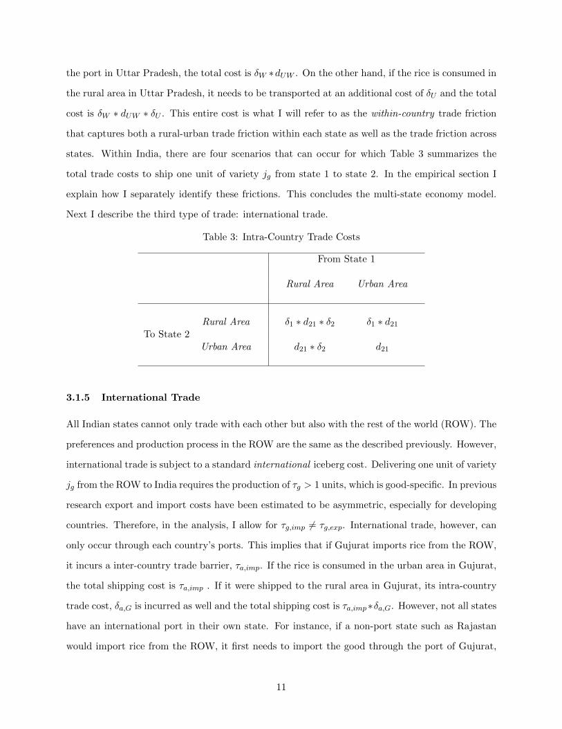
the port in Uttar Pradesh, the total cost is δW ∗dUW . On the other hand, if the rice is consumed in

the rural area in Uttar Pradesh, it needs to be transported at an additional cost of δU and the total

cost is δW ∗ dUW ∗ δU . This entire cost is what I will refer to as the within-country trade friction

that captures both a rural-urban trade friction within each state as well as the trade friction across

states. Within India, there are four scenarios that can occur for which Table 3 summarizes the

total trade costs to ship one unit of variety jg from state 1 to state 2. In the empirical section I

explain how I separately identify these frictions. This concludes the multi-state economy model.

Next I describe the third type of trade: international trade.

Table 3: Intra-Country Trade Costs

From State 1

Rural Area Urban Area

To State 2Rural Area δ1 ∗ d21 ∗ δ2 δ1 ∗ d21

Urban Area d21 ∗ δ2 d21

3.1.5 International Trade

All Indian states cannot only trade with each other but also with the rest of the world (ROW). The

preferences and production process in the ROW are the same as the described previously. However,

international trade is subject to a standard international iceberg cost. Delivering one unit of variety

jg from the ROW to India requires the production of τg > 1 units, which is good-specific. In previous

research export and import costs have been estimated to be asymmetric, especially for developing

countries. Therefore, in the analysis, I allow for τg,imp 6= τg,exp. International trade, however, can

only occur through each country’s ports. This implies that if Gujurat imports rice from the ROW,

it incurs a inter-country trade barrier, τa,imp. If the rice is consumed in the urban area in Gujurat,

the total shipping cost is τa,imp . If it were shipped to the rural area in Gujurat, its intra-country

trade cost, δa,G is incurred as well and the total shipping cost is τa,imp∗δa,G. However, not all states

have an international port in their own state. For instance, if a non-port state such as Rajastan

would import rice from the ROW, it first needs to import the good through the port of Gujurat,

11

which is the closest port, at international trade barrier, τa,imp. Then, it would be shipped from

Gujurat to Rajastan at an additional inter-state cost of dRG. If the rice is consumed in the urban

area in Rajastan, the total shipping cost is τa,imp ∗ dRG . If the rice is consumed in the rural

area in Rajastan, its intra-country trade cost, δR is incurred as well and the total shipping cost is

τa,imp ∗ dRG ∗ δR. By taking into account differential foreign market access across states, we can

have a better understanding of the different types of international integration and their potential

heterogeneous impact on trade and welfare. To summarize these trade costs, define Drg,sl as the

total trade cost faced in region r in state s for good variety jg imported from state l. It depends on

the region of consumption: urban and rural, the type of good: manufacturing and agriculture, and

whether state s is a port state. To see this more clearly, define state s as a non-port state and state

t as its nearest port state in India. Then the total trade costs of trading internationally for state t

and s are summarized in Table 4. If state t imports from the ROW, and the goods are consumed

in the urban area, the only cost incurred is the iceberg transportation cost. However, if goods are

consumed in the rural area they need to be transported at intra-state cost δs. For non-port state

s urban areas not only face the international trade cost but also the inter-state trade cost, dst , to

transport goods from the port state. Rural areas on the other hand pay an additional cost: the

intra-state trade barrier δs.

Table 4: International Trade Costs

From ROW

To To

Urban τg,imp Urban dst ∗ τg,impPort Non-Port

State t Rural δt ∗ τg,imp State s Rural δs ∗ dst ∗ τg,imp

In order to compute trade flows, I need to define region-specific prices within states across Indian

states and the ROW taking into account within and across state trade barriers and international

trade costs. As is standard in the literature, I assume that all markets are perfectly competitive.4

Then the price for good variety jg in region r in state s is:

4This is not a strong assumption as any price differences in the data could reflect market power in certain states.

12

prs (jg) = min {prsl (jg) ; l = 1...S,ROW}

where prsl (js) are different across across regions and states. We can summarize prices as follows:

prs (jg) = min

{wrsD

rg,sl

zs (jg); l = 1...S,ROW

}where Dr

g,sl is region- and good-specific and summarized in Table 4. Note that if both rural-urban

and inter-state trade barriers are set to one, the model reduces to the EK model. In fact, one can

interpret this model where countries are now defined as states within a country.

3.2 Equilibrium

For a given set of values for {βs}s=1..S,ROW , {Ts}s=1...S,ROW , Drg,sl, and {Ls}s=1..S,ROW , an equi-

librium is a set of region-good-state specific price indexes ,{P rg,s

}s=1..S,ROW

, region-state specific

wages {wrs}s=1...S,ROW , and good-specific bilateral trade flows Xg,sl such that:

1. Sector-state specific productivities follow a Frechet distribution

zs (jg) ∼ Fs (z) = exp(−Tg,sz−θg

)2. Consumers maximize utility (1).

3. Consumer’s purchase from the (trade cost inclusive) minimum cost producer.

4. Labor markets clear, i.e., total shipments from state s equal total production in state s.

All states within each country have a continuum of individuals who inelastically supply one unit of

labor. Let Ls be the population of state s of which βsLs is employed in agriculture and (1− βs)Ls

in manufacturing where βs ∈ [0, 1]. The price index for the CES objective function (1) is given by:

P rg,s =

[Γ

(θg + 1− σg

θg

)] 11−σg

[∑l

[Tg,l

(wrlD

rg,sl

)−θg]]− 1θg

(2)

where Γ is the Gamma function. A necessary condition for a finite solution is, therefore, (θg + 1) >

σg, g ∈ {a,m}. The spending of a typical consumer in region r in state s on good g is:

13

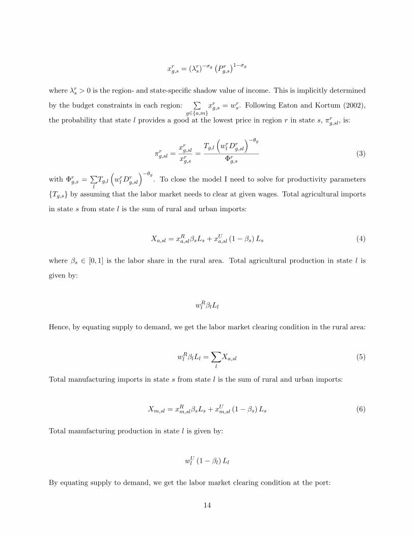
xrg,s = (λrs)−σg (P rg,s)1−σg

where λrs > 0 is the region- and state-specific shadow value of income. This is implicitly determined

by the budget constraints in each region:∑

g∈{a,m}xrg,s = wrs . Following Eaton and Kortum (2002),

the probability that state l provides a good at the lowest price in region r in state s, πrg,sl, is:

πrg,sl =xrg,slxrg,s

=Tg,l

(wrlD

rg,sl

)−θgΦrg,s

(3)

with Φrg,s =

∑l

Tg,l

(wrlD

rg,sl

)−θg. To close the model I need to solve for productivity parameters

{Tg,s} by assuming that the labor market needs to clear at given wages. Total agricultural imports

in state s from state l is the sum of rural and urban imports:

Xa,sl = xRa,slβsLs + xUa,sl (1− βs)Ls (4)

where βs ∈ [0, 1] is the labor share in the rural area. Total agricultural production in state l is

given by:

wRl βlLl

Hence, by equating supply to demand, we get the labor market clearing condition in the rural area:

wRl βlLl =∑l

Xa,sl (5)

Total manufacturing imports in state s from state l is the sum of rural and urban imports:

Xm,sl = xRm,slβsLs + xUm,sl (1− βs)Ls (6)

Total manufacturing production in state l is given by:

wUl (1− βl)Ll

By equating supply to demand, we get the labor market clearing condition at the port:

14

wUl (1− βl)Ll =∑l

Xm,sl (7)

Productivity parameters {Ts}s=1...S,ROW can be solved by equations (5) and (7). This completes

the statement of the model. To summarize, an economy is defined by a set of S states and one

ROW, each with two regions: a rural and an urban region. The rural area with a population βsLs

only produces agricultural goods and the urban area with population (1− βs)Ls only produces

manufacturing goods. Each region within a state has a specific wage {wrs} and location implied

by trade barriers{Drg,sl

}. Good g ∈ {a,m} is characterized by a technology parameters Tg,s and

θg . An equilibrium is a set of productivity parameters {Tg,s} that satisfies the market clearing

conditions (5) and (7).

4 Indian Trade Data and Patterns

To quantify the size and impact of intra-national versus inter -national country trade barriers, I

will estimate the model using the Indian economy. More concretely, the analysis in this paper is

based on annual state-level data collected by the Directorate General of Commercial Intelligence

and Statistics, part of the Ministry of Commerce and Industry in India for twelve month ending

on March 2012. There are two main data sets. The first is the “Inter-State Movements/Flows of

Goods by Rail, River and Air”. This data set contains state-level trade flows among 27 states in

India5, three union territories: Chandigarh, Puducherry and Delhi. The second set of data is the

“Foreign Trade Statistics of India (Principal Commodities and Country)” which contains foreign

imports and export data by country. More importantly, it provides information on foreign trade

through India’s major ports. Hence, these two data sets provide information on both intra-national

and inter -national trade flows which will identify their respective trade barriers. In the next section

I will elaborate on the data and how the model is estimated in more detail.

4.1 Indian Inter-State Trade

The Inter-State Movements/Flows of Goods by Rail, River and Air provides the trade flows for

inter-state trade. Trade flows are reported for each state origin, destination and commodity which

5Sikkim is not included in the inter state movement flow data.

15

identifies the inter-state trade costs, dsl. This data set also provides state-wise trade flows to and

from major ports. For instance, it reports commodity-wise trade from Bihar to “Andhra Pradesh

- Excluding Ports” and to “Andhra Pradesh - Ports”. This allows to separate domestic trade flows

from international trade flows. The mode of inter-state trade within India is mostly by rail. Air and

sea transportation across Indian states make up for less than 1% of total trade.6 Figure A.1 shows a

map of the Indian railway network which indicates Indian states seem to be well connected through

this network. Nevertheless, not every state is as well connected to the railway station. Figure A.2

shows access to the railway network in Jammu and Kashmir and Gujurat. Clearly railway density

is higher in Gujurat. To support this even further, the Data Portal of India produces summary

data on state-wise wholesale markets in India among which the distance to the nearest railway by

state. Table A.1 shows the median distance (in km) across all wholesale markets within each state.

This shows that there is large state heterogeneity in terms of market access which will be captured

by the intra-state friction, δs.

4.2 Indian International Trade

80% percent of India’s foreign trade goes through 21 main ports among which 14 seaports and 7

airports. Figure A.3 shows geographically where they are located. Clearly, the landlocked states

in the northern part of India are very remote from these major ports. Table 5 shows the trade

openness for each state for agriculture and manufacturing. Import and export openness are defined

as total foreign import and foreign exports, respectively, each divided by total production for either

agriculture and manufacturing.7 I break down the results for the major port states and the non-

port states.8 The first thing to notice here is that the observed trade patterns in the aggregate

data are still present: both port and non-port states are importing little agriculture.9 Secondly, all

international trade is driven by the port states, both for agriculture and manufacturing. Table 5,

6Currently, no comprehensive data on freight movement is available to indicate origin, destination, type and sizeof freight carried on roads by motorized transport.

7Note that is actual state trade with the rest of the world and not just the total amount of traffic that passesthrough these ports.

8The port states are include Andhra Pradesh, Delhi, Goa, Gujarat, Karnataka, Kerala, Maharashtra, Orissa,Tamil Nadu and West Bengal. The non-port states are Arunachal Pradesh, Assam, Bihar, Chandigarh, Chattishgarh,Haryana, Himachal Pradesh, Jammu and Kasmir, Jharkhand, Madhya Pradesh, Manipur, Meghalaya, Mizoram,Nagaland, Pondicheri and Karikal, Punjab, Rajasthan, Tripura, Uttar Pradesh and Uttaranchal.

9This is not driven by the fact that non-port states only produce agriculture. In fact, this patterns remain if Iuse state-wise GDP as the denominator.

16

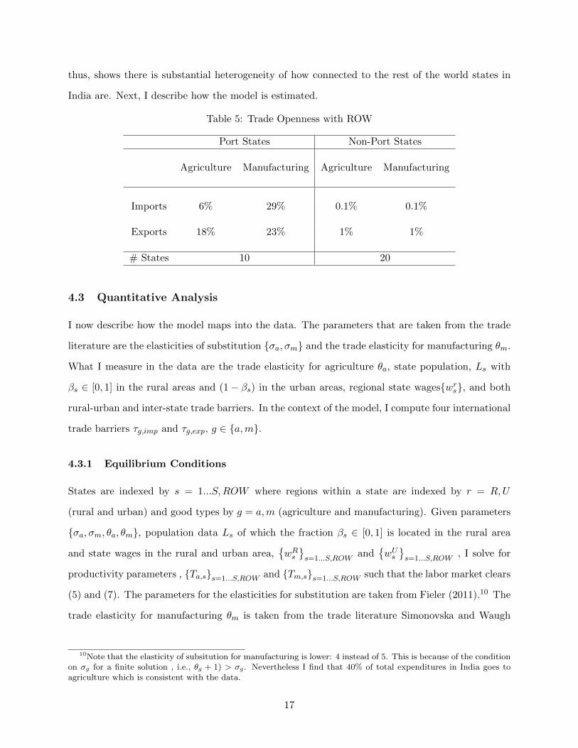
thus, shows there is substantial heterogeneity of how connected to the rest of the world states in

India are. Next, I describe how the model is estimated.

Table 5: Trade Openness with ROW

Port States Non-Port States

Agriculture Manufacturing Agriculture Manufacturing

Imports 6% 29% 0.1% 0.1%

Exports 18% 23% 1% 1%

# States 10 20

4.3 Quantitative Analysis

I now describe how the model maps into the data. The parameters that are taken from the trade

literature are the elasticities of substitution {σa, σm} and the trade elasticity for manufacturing θm.

What I measure in the data are the trade elasticity for agriculture θa, state population, Ls with

βs ∈ [0, 1] in the rural areas and (1− βs) in the urban areas, regional state wages{wrs}, and both

rural-urban and inter-state trade barriers. In the context of the model, I compute four international

trade barriers τg,imp and τg,exp, g ∈ {a,m}.

4.3.1 Equilibrium Conditions

States are indexed by s = 1...S,ROW where regions within a state are indexed by r = R,U

(rural and urban) and good types by g = a,m (agriculture and manufacturing). Given parameters

{σa, σm, θa, θm}, population data Ls of which the fraction βs ∈ [0, 1] is located in the rural area

and state wages in the rural and urban area,{wRs}s=1...S,ROW

and{wUs}s=1...S,ROW

, I solve for

productivity parameters , {Ta,s}s=1...S,ROW and {Tm,s}s=1...S,ROW such that the labor market clears

(5) and (7). The parameters for the elasticities for substitution are taken from Fieler (2011).10 The

trade elasticity for manufacturing θm is taken from the trade literature Simonovska and Waugh

10Note that the elasticity of subsitution for manufacturing is lower: 4 instead of 5. This is because of the conditionon σg for a finite solution , i.e., θg + 1) > σg. Nevertheless I find that 40% of total expenditures in India goes toagriculture which is consistent with the data.

17

(2014), and the trade elasticity for agriculture, θa, is estimated following methods in Simonovska

and Waugh (2014). The parameter values are given by Table 6.

Table 6: Parameter Values

Parameter Value

{σA, σM} {1.3, 4} Elasticity of substitution

{θa, θm} {5.1, 4} Cost-Elasticity of Trade Flows

The Ministry of Statistics and Program Implementation” in India.11 reports state-specific data

in India for 2014. It provides state-wise population, Ls. with 50% of the total population living

in non-port states. The rural population shares βs are computed as the percentage of the state-

wise population in rural areas in India. On average, the rural population represents 72% of the

total population, ranging from 68% in non-port states to 74% in port states. Agricultural and

manufacturing wages are proxied by the percent of value added in each sector divided by the

number of workers in each sector. For the rest of the world, the data are taken from UNIDO. Table

A.2 provides an overview of all the state-wise data. One main thing to note is that, on average,

wages in the urban areas are 3 times larger as in agriculture which is consistent with Restuccia

et al. (2008).

4.3.2 Inter-State Trade Barriers

In order to computeDrg,sl, I need to estimate both intra-country and inter-country trade barriers. As

described earlier, Drg,sl depends on the traded commodity g ∈ {a,m}, and where final consumption

takes place, i.e., in the rural or urban area. Inter-state frictions dsl are computed using a simple

no-arbitrage argument and disaggregated price data. The idea is that it must be the case that for

any given good g in two different states (s and l) within a country,ps(jg)pl(jg)

≤ dsl, otherwise there

would be an arbitrage opportunity. Therefore, an estimate of dsl is the maximum of relative prices

over good variety jg. In other words:

log dsl = max 2jg

log {ps (jg)− pl (jg)} (8)

11See http://planningcommission.nic.in/.

18

where max 2 represent the second highest price difference which alleviates measurement error con-

cerns. Prices for Indian agricultural goods are published by the Data Portal India.12 This data set

consists of state-, market-, and variety-specific wholesale prices of 110 different agricultural goods

across 1850 markets for 2012. Figure A.3 shows a map of all the wholesale markets located in

Andhra Pradesh. It provides the daily maximum price, minimum price and modal price. I first

average out modal prices by month and year for each market good variety. Then, to measure

the inter-state trade costs in India, I use a market average price within state for each good vari-

ety. I then compute inter-state trade costs for each state-pair in India using the second highest

price differential across each good variety. Hence I calculate 30 ∗ 30 − 30 across state trade costs.

Figure 2 shows a histogram of these frictions. The median trade cost is 2.63. If I compute this

same median friction using similar USDA data in the U.S. USDA data can be downloaded from

http://quickstats.nass.usda.gov/. I find a median trade cost one 1.28, which is around one sixth

of the Indian trade costs and around the same magnitude as other micro evidence has estimated.

This is suggestive of relatively large trade frictions across Indian states.

Figure 2: Trade Cost Histogram (2012)

(a) India (b) U.S.

4.3.3 Intra-State Trade Barriers

As mentioned before, each state has differential access to the nearest railway station varying from

247 km in Jammu and Kashmir to 3 km in Delhi. Although there is a correlation between average railway

12This data set is generated through the AGMARKNET Portal http : //agmarknet.nic.in.

19

access and state area, it is not perfect. For instance, Jammu and Kashmir has an area of 222,236 km2

which is similar to Gujurat with an area of 196,021 km2, the distance to the nearest railway station is 247

km in the former and 12 km in the latter. Therefore, I construct a measure for the intra-state cost using

the same method described in the section before but now using the cross-market price variation. Again, I

first average out modal prices by month and year for each market good variety. But then I find

the second highest price differential across wholesale markets within each state. Hence, I compute

30 intra-state trade costs which represents the δs in the model. I find a median intra-state trade

cost of 1.1 for port states and 1.2 for non-port states which are around half of the inter-state trade

cost is the U.S. This suggests that non-port states are not only constrained from foreign market

access but are less integrated within state as well. Moreover computed price differentials are highly

correlated with the distance to the port with a correlation coefficient of 0.62.

4.3.4 International Trade Barriers

Finally, I estimate the international trade barriers as follows. I assume there is one other country

that each state in India trades with , i.e., the rest of the world. Let zg,sROW =Xg,sROW

Xg,sXg,ROWbe the

state- and good specific import value from the rest of the world for good g ∈ {a,m}, normalized

by the product of the total income. Similarly, define zg,ROWs =Xg,ROWs

Xg,sXg,ROWas the state- and

good specific export value from the state in India to the rest of the world for good g ∈ {a,m},

normalized by the product of the total income. Given the computed intra-state and inter-state

trade costs I compute the total inter-country trade costs by matching good specific total foreign

trade. To do so, I assume that all foreign imports and exports go through a main port shown in

Figure A.4. For example, if Arunachal Pradesh exports to the rest of the world, the goods need

to get shipped through the port of West Bengal. Using the previously calculated intra-state costs

δs and inter-state trade costs dsl, I compute the total intra-country trade cost of shipping goods

to the nearest port. Then, I assume that once the goods are at the port, export and import costs

are the same across ports but not across goods. In other words I estimate four international trade

costs: an agricultural and manufacturing import and export costs denoted by τa,imp, τm,imp, τa,exp

and τm,exp respectively to minimize∑s

∑gzg,sROW +

∑s

∑gzg,ROWs.

Table 7 shows the trade costs that fit the model best. Note that these are the border costs,

i.e., the trade costs the urban areas in port states. Later, I will discuss how large the trade costs

20

are that the rural areas face in all states. In fact, the trade costs confirm what the literature has

found on explaining international trade patterns between rich and poor countries. First, the export

costs for manufacturing are substantially higher than the import costs. This is consistent with

Waugh (2010) where he finds that to reconcile international trade patterns and prices, it has to

be that poor countries face large export costs. Second, I find that the import cost for agriculture

are about 4 times larger than for manufacturing. This is in line with the results Tombe (2014)

found. However, the innovation of this paper is to allow for heterogeneity in terms of port access

and hence foreign market access.

Table 7: Border Iceberg Trade Costs

Import Export

Agriculture 2.9 2.3

Manufacturing 1.5 4.3

Table 8 shows the main moments in the data and I compare them to the model predictions.

The first column shows the same export and import openness as Table 5 whereas the second

column shows the results of the model, taking into account states have differential port access.

Comparing the model outcomes to the data, the model performs very well. Note that the import

and export border costs are kept constant across states, and the only difference between port and

non-port states is the access to an international port. Still, the model captures the large trade

Table 8: Model Moments

Agriculture Manufacturing

Data Model Data Model

Port StatesImports 6% 7% 29% 34%

Exports 18% 18% 23% 18%

Non-Port StatesImports 0.1% 0.3% 0.1% 2%

Exports 1% 1% 1% 1%

21

differences across port and non-port states in terms of magnitudes. For instance, non-port states

export 18% of total agricultural production whereas non-port states only export 1%. Moreover, the

model captures that port states both import and export substantially more manufacturing than

agriculture, whereas for non-port states this is not the case. For example, port states import 6% of

total agricultural production whereas they import 23% of total manufacturing production. Hence,

taking into account differential port access is quantitatively important in order to explain state-wise

international trading patterns with non-port states trading substantially less than port states.

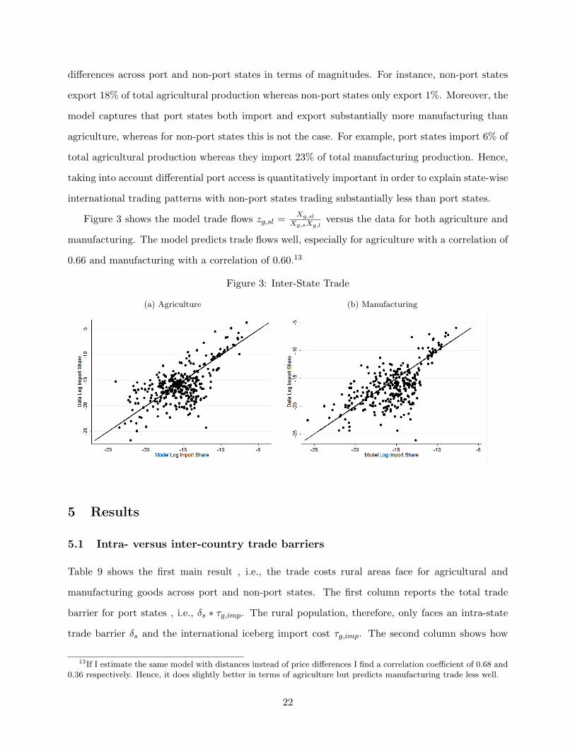
Figure 3 shows the model trade flows zg,sl =Xg,sl

Xg,sXg,lversus the data for both agriculture and

manufacturing. The model predicts trade flows well, especially for agriculture with a correlation of

0.66 and manufacturing with a correlation of 0.60.13

Figure 3: Inter-State Trade

(a) Agriculture (b) Manufacturing

5 Results

5.1 Intra- versus inter-country trade barriers

Table 9 shows the first main result , i.e., the trade costs rural areas face for agricultural and

manufacturing goods across port and non-port states. The first column reports the total trade

barrier for port states , i.e., δs ∗ τg,imp. The rural population, therefore, only faces an intra-state

trade barrier δs and the international iceberg import cost τg,imp. The second column shows how

13If I estimate the same model with distances instead of price differences I find a correlation coefficient of 0.68 and0.36 respectively. Hence, it does slightly better in terms of agriculture but predicts manufacturing trade less well.

22

Table 9: Intra- versus inter-country trade cost

Port States Non-Port States

Total Cost % Intra-country Total Cost % Intra-countryδs ∗ τg,imp δs δs ∗ dsl ∗ τg,imp δs ∗ dsl

Agriculture 3.3 5% 7.2 41%

Manufacturing 1.7 18% 3.6 71%

muchFigure 4: Intra-Country Trade Frictions (%)

x

much of the total cost is the intra-state trade cost in percent. I find that, on average, the total

trade cost is 3.3 in agriculture and 1.7 in manufacturing where intra-state trade costs represent 5%

23

and 18% respectively. The last two columns present the total trade cost for the non-port states,

δs ∗ dsl ∗ τg,imp, and the percentage of their total intra-country trade cost. The intra-country trade

cost comprises of the cost to ship from the port state to the urban area, dsl, and the intra-state

trade cost to import from the urban to the rural area, δs. I find that, on average, the total trade

cost is more than triple for non-port states: 7.2 in agriculture and 3.6 in manufacturing. Moreover,

the percentage of the intra-country trade frictions for these states makes up 41% and 71% of the

total trade cost in agriculture and manufacturing respectively. Hence, for non-port states, within

country trade cost are substantial. Figure 4 shows this graphically. Clearly, as states are further

removed from a major port, the intra-country trade friction increases, going up to 61% in Jammu

and Kashmir.

5.2 Counterfactuals

With the calibrated model, I now analyze counterfactual experiments. The procedure is as follow:

given the same state population, Ls, rural population shares βs, parameter values σa, σm, θa, θm,

and the productivity vectors Ta,s and Tm,s, I change a specific trade costs. Then, I recalculate

wages in the urban and rural areas for each state such that labor markets clear given by equations

(5) and (7). Welfare is measured as the change in total utility, consistent with the literature. In

this setup indirect utility for an representative agent in region r in state s is (see Appendix for

derivation):

U rs = λrs

[(σa

σa − 1

)xrs,a +

(σm

σm − 1

)xrs,m

]where xra and xrm represent region specific expenditures on agriculture and manufacturing respec-

tively. In a standard EK model welfare is typically calculated as the real wages, wP, where P is

given by λ−1 which is the shadow value of income. In this setup we have a similar expression where

λrs represents an inverse price index and(

σaσa−1

)xrs,a +

(σmσm−1

)xrs,m is similar to the wages in each

region, i.e., xra + xrm. However, there is a higher value on the agricultural expenditures due to the

non-homotheticity. Total state welfare is then given by the sum of rural and urban welfare, i.e., :

Us = λRs

[(σa

σa − 1

)xRs,a +

(σm

σm − 1

)xRs,m

]βsLs+λ

Us

[(σa

σa − 1

)xUs,a +

(σm

σm − 1

)xUs,m

](1− βs)Ls

(9)

24

5.2.1 Decreasing international import barrier

The first policy experiment is to completely reduce international import costs , i.e., τa,imp =

τm,imp = 1. The results are shown in Table 10 for the aggregate population and separately for

port states and non-port states. Column (1) shows that after a reduction in import barriers, total

agricultural imports would increase by more than 800%. It shows that in the aggregate agricultural

imports as a fraction of production would increase by six percentage points compared to the baseline.

Overall welfare, given by equation (9), increases by 7%. This is due to the fact that, although rural

areas are worse off due to higher competition, the urban areas are really benefiting from lower

cost agriculture which outweighs the welfare losses experienced in the rural areas. In the non-port

states the urban consumers are also benefiting from cheaper agricultural products. However, their

welfare gains are not as large because agricultural imports did not increase drastically as it did for

the port states. Breaking these results down by port and non-port states, we can see that most

of these aggregate results are driven by the port states: welfare increases by 13% in port states

compared to 1% in non-port states. This shows that policies focused at reducing border costs can

have very heterogeneous effects on states depending on port access.

5.2.2 Building a port in every non-port state

As was clear from Figure A.4, not every state has a major port and in fact, the previous section

showed that transporting goods to and from the port is quantitatively relevant. Therefore, the

second counterfactual is to estimate the impact of having an international port in all states, thereby

increasing market access to the rest of the world. In the model, we reduce the inter-state trade

barrier dsl to one, only for those states with no major ports and keeping the inter-state country

trade costs to trade within India constant. The results are shown in the second column in Table

10. Overall, total welfare increases by 2% which is now mostly driven by the welfare gains in

non-port states: 3%. If we compare these outcomes for ports versus non-ports clearly agricultural

imports as a fraction of production increased substantially for non-port states: from 0.9% to 15%

whereas for port states it increased from 8% to 12%. In terms of welfare, port states are now

worse off than the baseline whereas welfare has increased by 3% for non-port states. The reason

for the welfare loss in port states is double: one the hand, rural areas are faced with more foreign

25

Table 10: The Effect of Inter- versus Intra-country Trade Costs

Baseline (1) (2) (3) (4)

Aggregate %Agricultural Imports

Production5% 20% 14% 3% 4%

%4 Total Welfare - 7% 2% 15% 5%

Port States %Agricultural Imports

Production8% 38% 12% 3% 7%

%4 Total Welfare - 13% -0% 12% 4%

Non-Port States %Agricultural Imports

Production0.9% 6% 15% 1.3% 0.7%

%4 Total Welfare - 1% 3% 18% 6%

Note: The first column shows the baseline values for the calibrated model. Column (1) presents the impact

of a full reduction in international import cost, column (2) shows the results for building a port in non-

port states. Column (3) presents the impact of reducing inter-state trade cost to the U.S. level and column

(4) shows the impact of reducing intra-state trade costs to the lowest level across Indian states.

competition which leads to lower real income in those areas. The negative welfare loss in the

urban areas on the other hand, is due to international changes in manufacturing. Since ports have

been built in non-port states, their manufacturing trade is also increasing. Hence, the non-port

states are importing substantially less from those states which leads to an increase in nominal

manufacturing wages. However, manufacturing prices are increasing relatively more and offsets the

nominal manufacturing wage increase. Hence, the urban area in port states is relatively poorer.

The non-port states, on the other hand are benefiting on the whole. Although rural areas are losing

real income, the urban areas now have access to relatively cheaper agricultural and manufacturing

products which increases their real income.

5.2.3 Reduce inter-state trade costs

The following counterfactuals will be focused on regional integration and their impacts. First, I

consider the impact of reducing inter-state trade barriers. In the model, we divide all inter-state

costs, dsl, by six in order to have a reasonable comparison with the U.S.. This would coincide

26

with building a more sophisticated railway network. The results are summarized in column (3).

First, overall imports actually decrease. This is driven by the fact that the port states decrease

international imports from 6% to 4% of total production. For non-port states international imports

increase very modestly. However, the most stark difference is the impact on welfare which is a 15%

increase overall which is substantially larger than any of the international integration policies. The

intuition is that there are large barriers to trade within India which forces the port states to import

more from the rest of the world. However, after reducing these trade barriers, the urban areas are

really benefiting from lower prices for both agriculture and manufacturing. The rural areas are also

benefiting from increased trade which leads nominal wages to increase in both regions while prices

go down which leads to an overall increase in welfare. These effects seems to be even larger for

non-port states which tended to be more isolated.

5.2.4 Reduce intra-state trade costs

Finally, I analyze the impact of increased intra-state market access which reflects the rural urban

connection. Table A.1 showed that intra-state trade costs are very different across states and this

is a more severe issue for the northern landlocked states. Hence, the counterfactual experiment is

to provide a better railway network in each state in order to reduce those intra-state frictions. In

the model, I set all rural-urban costs, δs, equal to one. Column (4) in Table 10 shows the results.

Agricultural imports from the rest of the world change very little for both port states and non-port

states. This is due to the fact that markets within India are becoming more integrated, especially the

rural areas. They are benefiting from cheaper manufacturing goods and urban areas are benefiting

from cheaper agricultural products. Overall welfare goes up by 5% which is comparable to fully

reducing import barriers. This suggests that are large potential welfare gains from connecting rural

and urban areas. However, the overall welfare increase is smaller compared to connecting states in

India through decreasing inter-state trade costs.

6 Conclusion

The goal of this paper is to this paper is to quantify the size of inter-country versus intra-country

trade barriers and assess the impact on patterns of trade and welfare. I have developed a quanti-

27

tative multi-sector international trade model featuring non-homothetic preferences in which states

trade both within country and internationally. I calibrate it to the Indian economy using foreign

and domestic trade flows at the Indian state level. I find that domestic trade frictions make up a

substantial part of the total trade cost: on average they account for 30% with large heterogeneity

depending on the distance to the closest port. Secondly, I found that the welfare impacts of reduc-

ing inter-state trade barriers are substantially larger than completely reducing agricultural import

costs: 15% versus 7%. In other words India has more to gain from trading with itself compared to

trading with the rest of the world.

In future work, I would like to apply this analysis to African countries. Promoting cross-

African trade been a major policy focus resulting in, for instance, different monetary unions across

geographic regions. However, trade has been lagging and quantifying the main barriers behind

these trade patterns in the context of cross-country and within country trade barriers, therefore, is

an important avenue for future research.

References

Adamopoulos, T. (2011): “Transportation Costs, Agricultural Productivity, and Cross-Country

Income Differences,” International Economic Review, 52, 489–521.

Alessandria, G. and J. P. Kaboski (2011): “Pricing to Market and the Failure of Absolute

PPP,” American Economic Journal: Macroeconomics, 3, 91–127.

Allen, T. (2014): “Information Frictions in Trade,” Econometrica, forthcoming.

Allen, T. and C. Arkolakis (2014): “Trade and the Topography of the Spatial Economy,”

Quarterly Journal of Economics, 129, 1085–1140.

Alvarez, F. and R. E. Lucas (2007): “General Equilibrium Analysis of the Eaton-Kortum

Model of International Trade.” Journal of Monetary Economics, 54, 1726–1768.

Arkolakis, C., A. Costinot, and A. Rodrıguez-Clare (2011): “New Trade Models, Same

old Gains?” The American Economic Review, 102, 94–130.

28

Asturias, J., M. Garcıa-Santana, and R. Roberto (2014): “Competition and the welfare

gains from transportation infrastructure: Evidence from the Golden Quadrilateral of India,”

Working paper.

Atkin, D. and D. Donaldson (2014): “Who’s Getting Globalized? The Size and Impact of

Intranational Trade Costs,” Working paper.

Behrens, K., C. Gaigne, G. I. P. Ottaviano, and T. Jacques-Francois (2006): “Is re-

moteness a locational disadvantage?” Journal of Economic Geography, 6, 347–368.

Bureau of Transportation Statistics (2012): “Commodity Flow Survey,” .

Caron, J., T. Fally, and J. R. Markusen (2014): “International Trade Puzzles: A Solution

Linking Production and Preferences,” Quarterly Journal of Economics, forthcoming.

Caselli, F. (2005): “Accounting for Cross-Country Income Differences,” Handbook of Economic

Growth, 1, 679–741.

Cocar, A. K. and P. D. Fajgelbaum (2014): “Internal Geography, International Trade, and

Regional Outcomes,” Working paper.

Crucini, M. J. and M. Shintani (2008): “Persistence in law of one price deviations: Evidence

from micro-data.” Journal of Monetary Economics, 55, 629–644.

Data Portal of India (2012): “Agricultural Marketing Information Network,” .

Directorate General of Commercial Intelligence and Statistics, Ministry of Com-

merce and Industry, Governments of India, 565, Anandapur; Ward-108; Plot no-

22; Sec-I , ECADP, Kolkata - 700 107, India. (2012): “The Inter-State Movements/Flows

of Goods by Rail, River and Air,” .

Donaldson, D. (2014): “Railroads of the Raj: Estimating the Impact of Transportation Infras-

tructure,” The American Economic Review, forthcoming.

Donaldson, D. and R. Hornbeck (2014): “Railroads and American Economic Growth: A

Market Access Approach,” Working paper.

29

Dornbusch, R., S. Fischer, and P. A. Samuelson (1977): “Comparative Advantage, Trade,

and Payments in a Ricardian Model with a Continuum of Goods.” The American Economic

Review, 67, 823–839.

Eaton, J. and S. Kortum (2002): “Technology, Geography, and Trade,” Econometrica, 70,

1741–1779.

Engel, C. and J. H. Rogers (1996): “How Wide Is the Border?” The American Economic

Review, 86, 1112–25.

Feenstra, R. C. and D. E. Weinstein (2010): “Globalization, Markups, and the U.S. Price

Level,” Working paper.

Fieler, A. C. (2011): “Nonhomotheticity and bilateral trade: Evidence and a quantitative expla-

nation,” Econometrica, 79, 1069–1101.

Food and Agriculture Organization of the United Nations (2012): “Agricultural Pro-

ducer Prices,” .

Gollin, D., D. Lagakos, and M. Waugh (2014): “The Agricultural Productivity Gap in Poor

Countries,” Quarterly Journal of Economics, 129, 939–993.

Gollin, D. and R. Rogerson (2014): “Productivity, Transport Costs, and Subsistence Agricul-

ture,” Journal of Development Economics, 107, 38–48.

Hummels, D. and G. Schaur (2013): “Time as a Trade Barrier,” American Economic Review,

103, 1–27.

Jensen, R. (2007): “The digital provide: information (technology), market performance, and

welfare in the South Indian Fisheries Sector,” Quarterly Journal of Economics, 122, 879–924.

Limao, N. and A. J. Venables (1999): “Infrastructure, Geographical Disadvantage, and Trans-

port Costs, and Trade,” The World Bank Economic Review, 15, 451–479.

Parsley, D. C. and S.-J. Weib (2001): “Explaining the Border Effect: The Role of Exchange

Rate Variability, Shipping Costs, and Geography,” Journal of International Economics, 55, 87–

105.

30

Ramondo, N., A. Rodrıguez-Clare, and M. Saborıo-Rodrıguez (2014): “Trade, Domestic

Frictions, and Scale Effects.” Working paper.

Restuccia, D., D. T. Y. Yang, and X. Zhu (2008): “Agriculture and aggregate productivity:

A quantitative cross-country analysis,” Journal of Monetary Economics, 55, 234–250.

Rossi-Hansberg, E. (2005): “A Spatial Theory of Trade,” American Economic Review, 95, 1464–

1491.

Simonovska, I. and M. Waugh (2014): “The Elasticity of Trade: Estimates and Evidence.”

Journal of International Economics, 92, 34–50.

Sotelo, S. (2014): “Trade Frictions and Agricultural Productivity: Theory and Evidence from

Peru,” Working paper.

Storeygard, A. (2014): “Farther on down the road: transport costs, trade and urban growth in

sub-Saharan Africa.” Working paper.

Tombe, T. (2014): “The Missing Food Problem.” American Economic Journal: Macroeconomics,

forthcoming.

United Nations (2012): “UN Commodity Trade Statistics Database,” .

United Nations Word Food Program (2012): “VAM Food and Commodity Prices Data

Store,” .

United States Department of Agriculture (2012): “National Aggregate Statistics Service

in the Agricultural Prices,” .

Waugh, M. (2010): “International Trade and Income Differences,” The American Economic Re-

view, 99, 2093–2124.

31

Appendix

Figure A.1: India’s Railway Network

32

Figure A.2: Railway Network Access

(a) Jammu and Kashmir Railway Network

(b) Gujurat Railway Network

33

Table A.1: Median Market Distance to nearest railway

Distance (km)

Andhra Pradesh 24

Arunachal Pradesh 91

Assam 41

Bihar 8

Chandigarh 5

Chattishgarh 44

Delhi 3

Goa 14

Gujarat 12

Haryana 9

Himachal Pradesh 48

Jammu and Kashmir 247

Jharkhand 20

Karnataka 25

Kerala 33

Madhya Pradesh 33

Maharashtra 34

Manipur 342

Meghalaya 112

Mizoram 224

Nagaland 137

Orissa 42

Pondicheri and Karikal 11

Punjab 11

Rajasthan 10

Tamil Nadu 14

Tripura 147

Uttar Pradesh 10

Uttaranchal 13

West Bengal 17

34

Figure A.3: Wholesale Markets in Andhra Pradesh

35

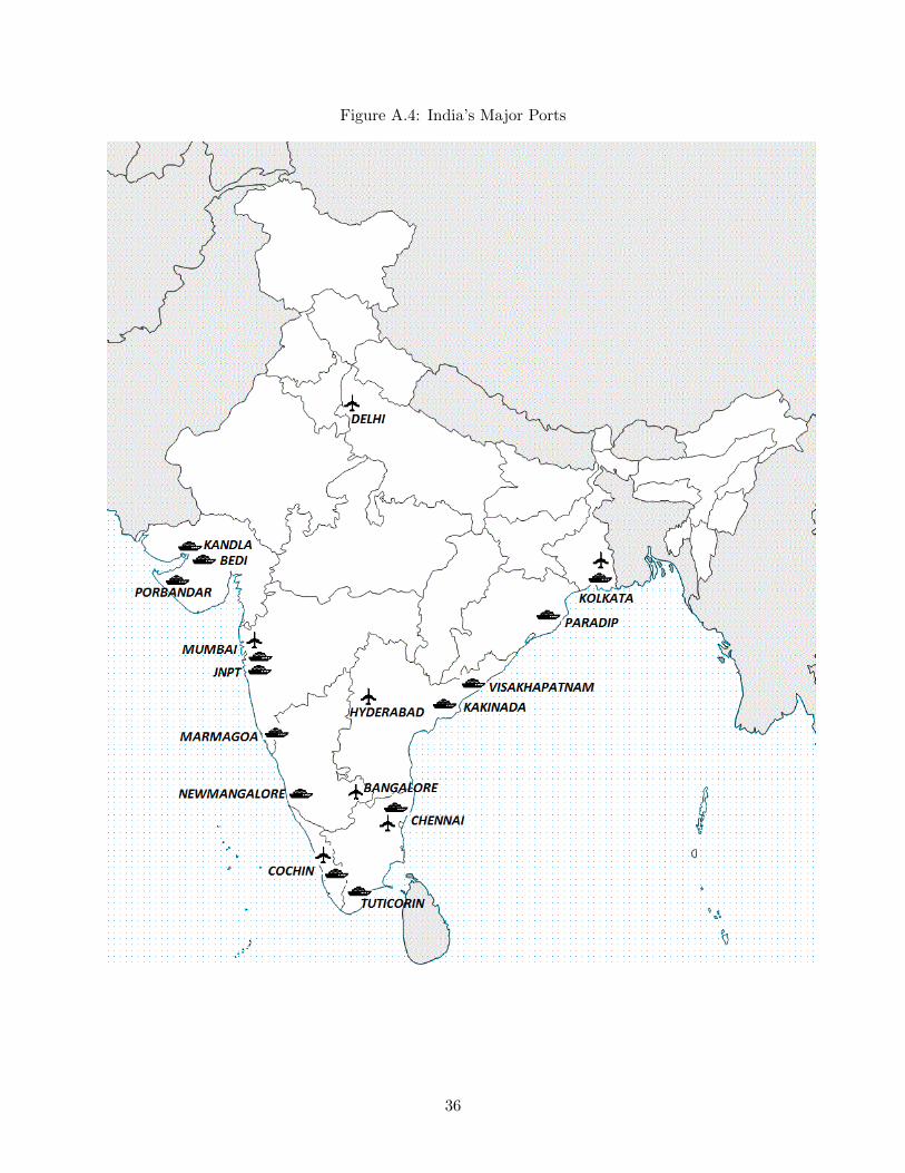
Figure A.4: India’s Major Ports

36

Table A.2: Data Model

Population Share Rural Pop. (β) Rural wage wRs Urban wage wU

s

Andhra Pradesh 84,665,533 67% 0.19 0.54

Arunachal Pradesh 1,382,611 77% 0.21 0.85

Assam 31,169,272 86% 0.09 0.50

Bihar 103,804,637 89% 0.05 0.32

Chandigarh 1,054,686 3% 0.27 0.27

Chattishgarh 25,540,196 77% 0.10 0.81

Delhi 16,753,235 3% 0.49 0.27

Goa 1,457,723 38% 0.29 1.98

Gujarat 60,383,628 57% 0.21 0.62

Haryana 25,353,081 65% 0.29 0.81

Himachal Pradesh 6,856,509 90% 0.14 0.72

Jammu and Kasmir 12,548,926 73% 0.10 0.45

Jharkhand 32,966,238 76% 0.06 0.55

Karnataka 61,130,704 61% 0.15 0.44

Kerala 33,387,677 52% 0.20 0.36

Madhya Pradesh 72,597,565 72% 0.11 0.37

Maharashtra 112,372,972 55% 0.18 0.62

Manipur 2,721,756 70% 0.10 0.30

Meghalaya 2,964,007 80% 0.08 0.64

Mizoram 1,091,014 48% 0.16 0.19

Nagaland 1,980,602 71% 0.29 0.30

Orissa 41,947,358 83% 0.09 0.96

Pondicheri and Karikal 1,244,464 32% 0.08 0.55

Punjab 27,704,236 63% 0.34 0.51

Rajasthan 68,621,012 75% 0.14 0.51

Tamil Nadu 72,138,958 52% 0.16 0.45

Tripura 3,671,032 74% 0.10 0.51

Uttar Pradesh 199,581,477 78% 0.09 0.28

Uttaranchal 10,116,752 69% 0.13 0.90

West Bengal 91,347,736 68% 0.15 0.28

Rest of World (ROW) 579,144,440,361,130,704 40% 1 1.88

37

Table A.3: Total Agricultural Trade Cost

Port Total Trade % Intra-country Non-Port Total Trade % Intra-country

States Cost States Cost

δs ∗ τa,imp δs δs ∗ dsl ∗ τa,imp δs ∗ dslAverage 3.33 5.2% Average 7.26 41%

Andhra Pradesh 3.30 4.8% Arunachal Pradesh 7.56 43%

Delhi 3.05 0.8% Assam 7.28 42%

Goa 3.09 1.5% Bihar 4.54 20%

Gujarat 3.18 3.0% Chandigarh 7.23 41%

Karnataka 3.82 12% Chattishgarh 6.17 35%

Kerala 3.49 7.6% Haryana 8.77 49%

Maharashtra 3.37 5.8% Himachal Pradesh 10.5 56%

Orissa 3.63 9.5% Jammu and Kashmir 12.5 61%

Tamil Nadu 3.36 5.7% Jharkhand 13.2 63%

West Bengal 3.21 3.4% Madhya Pradesh 5.34 28%

Manipur 5.25 27%

Meghalaya 13.7 64%

Mizoram 9.36 51%

Nagaland 5.33 28%

Pondicheri 4.80 23%

Punjab 9.11 50%

Rajasthan 6.29 35%

Tripura 4.85 24%

Uttar Pradesh 4.78 23%

Uttaranchal 10.5 56%

Note: This Table shows the total import cost for agricultural goods faced by the rural areas. It shows the state-specific

total import cost and the percentage of the within-country trade cost. The first three columns show the results for all the

port states and the last three columns show the results for all the non-port states.

38

Table A.4: Total Manufacturing Trade Cost

Port Total Trade % Intra-country Non-Port Total Trade % Intra-country

States Cost States Cost

δs ∗ τm,imp δs δs ∗ dsl ∗ τm,imp δs ∗ dslAverage 1.66 18% Average 3.63 71%

Andhra Pradesh 1.65 17% Arunachal Pradesh 3.78 75%

Delhi 1.53 3% Assam 3.64 74%

Goa 1.54 6% Bihar 2.27 51%

Gujarat 1.59 11% Chandigarh 3.62 74%

Karnataka 1.91 35% Chattishgarh 3.09 68%

Kerala 1.75 24% Haryana 4.39 79%

Maharashtra 1.68 20% Himachal Pradesh 5.24 83%

Orissa 1.81 30% Jammu and Kashmir 6.26 86%

Tamil Nadu 1.68 19% Jharkhand 6.65 87%

West Bengal 1.61 12% Madhya Pradesh 2.67 61%

Manipur 2.63 60%

Meghalaya 6.88 88%

Mizoram 4.68 81%

Nagaland 2.67 61%

Pondicheri 2.40 55%

Punjab 4.56 80%

Rajasthan 3.14 69%

Tripura 2.43 55%

Uttar Pradesh 2.39 54%

Uttaranchal 5.27 83%

Note: This Table shows the total import cost for manufacturing goods faced by the rural areas. It shows the state-specific

total import cost and the percentage of the within-country trade cost. The first three columns show the results for all the

port states and the last three columns show the results for all the non-port states.

39

Appendix (not for publication)

Welfare is measured by the change in utility. Recall that a representative agent in region r in

state s chooses the quantity consumed of both agricultural and manufacturing goods of variety jg,

denoted by {q (jg)}jg∈[0,1] , g ∈ {a,m} to maximize:

maxqrs(ja)≥0,qrs(jm)≥0

(σa

σa − 1

) 1

0

[qrs (ja)

σa−1σ1

]dja +

(σm

σm − 1

) 1

0

[qrs (jm)

σm−1σm

]djm

s.t.1

0

qrs (ja) prs (ja) dja +

1

0

qrs (jm) prs (jm) djm = wrs

The first-order necessary conditions are given by:

qrs (ja)σa−1σa−1 = λrsp

rs (ja)

qrs (jm)σm−1σm

−1 = λrsprs (jm)

1

0

qrs (ja) prs (ja) dja +

1

0

qrs (jm) prs (jm) djm = wrs

Multiplying the first two first-order necessary conditions by qrs (ja) implies:

qrs (ja)σa−1σa = λrsp

rs (ja) q

rs (ja)

qrs (jm)σm−1σm = λrsp

rs (jm) qrs (jm)

1

0

qrs (ja) prs (ja) dja +

1

0

qrs (jm) prs (jm) djm = wrs

40

Then, integrating the first two expressions over all varieties implies:

1

0

qrs (ja)σa−1σa dja = λrs

1

0

prs (ja) qrs (ja) dja

1

0

qrs (jm)σm−1σm djm = λrs

1

0

prs (jm) qrs (jm) djm

1

0

qrs (ja) prs (ja) dja +

1

0

qrs (jm) prs (jm) djm = wrs

Substitute these expressions into the objective function in order to obtain the indirect utility:

U =

(σa

σa − 1

)λrs

1

0

qrs (ja) prs (ja) dja +

(σm

σm − 1

)λrs

1

0

qrs (jm) prs (jm) djm

= λrs

( σaσa − 1

) 1

0

qrs (ja) prs (ja) dja +

(σm

σm − 1

) 1

0

qrs (jm) prs (jm) djm

= λrs

[(σa

σa − 1

)xrs,a +

(σm

σm − 1

)xrs,m

]

where

xrs,g =

1

0

qrs (jg) prs (jg) djg

is defined as the state-region-specific expenditure on good variety jg.

41