A. Piccato, A.Egidi, D. Corona, A.Balsamo

Freeform scanning on the internal involute waviness measurement standard

T.R. 17/2017 September 2017

I.N.RI.M. TECHNICAL REPORT

Abstract

PTB designed and manufactured an internal involute waviness scanning measurement standard (SAFT 2w). The device embodies an internal and an external involute profile both superposed with a certain waviness which enables to characterize the dynamic behavior of probing systems. The measurement standard is designed as a disc with two high accurate reference surfaces (a circle and a plane) to define the datum axis of the workpiece. A precise bore is used to define the x-axis. Both the internal and external involute profiles have been calibrated as unmodified gear profiles according to existing standards and guidelines (e.g. ISO 1328-1), i.e. for both profiles the total deviation Fa, the form deviation ffa and the slope deviation fHa have been calibrated. Moreover, a spectral analysis has been performed using FFT method. The three main components of the spectrum have been calibrated in terms of wavelength and amplitude. INRIM has investigated the influence of scanning parameter such as 5 different scanning speeds within the range of the machine specification, 3 different workpiece orientations inside the measurement volume and 3 different stylus lengths. The measurement have been carried out on the CMM at INRIM by using the internal involute waviness measuring the calibrated standard SAFT 2w and a model for estimating the measuring uncertainty contribution has been derived from the measurement results. This work is related to the deliverable 5.2.3 of Drive Train Poject (ENG56).

Il PTB ha progettato e costruito un campione envolvente (SAFT 2w) per la valtazione degli effetti introdotti dai parametri di scanning nelle misure a coordiante. Il dispositivo comprende un profilo di evolvente interna ed esterna, entrambe sovrapposte con una certa waviness (una lavorazione meccanica che riproduce un andamento ondoso sulla superficie del pezzo con determinate caratteristiche di lunghezza d’onda e ampiezza) che consente di caratterizzare il comportamento dinamico dei sistemi di scansione. Il campione di misura è progettato come un disco con due superfici di riferimento ad alta precisione (un cerchio e un piano) per definire l'asse di riferimento del pezzo. Un foro di precisione viene utilizzato per definire l'asse x. Entrambi i profili di evolvente sono stati tarati come profili di ruote dentate secondo gli standard e le linee guida esistenti (si veda ad esempio ISO 1328-1). Per entrambi i profili sono state tarate la deviazione totale

F, la deviazione modulo ff e la deviazione della pendenza fH. Inoltre, è stata effettuata un'analisi spettrale usando il metodo FFT. Le tre componenti principali dello spettro sono state tarate (PTB) in termini di lunghezza d'onda e di ampiezza. L’INRIM ha analizzato l'influenza dei parametri di scansione, quali: 5 diverse velocità di scansione (da 2 mm / s a 24 mm / s), 3 diversi orientamenti del pezzo all'interno del volume di misura e 3 diverse lunghezze dello stilo (35 mm, 135 mm e 235 mm). Il risultato delle misure è stato analizzato per valutare, per entrambi i

profili, le deviazioni F, ff and fH) secondo la ISO 1328-1: 2013 e l'influenza dovuta alle variabili di scansione. Questo lavoro si colloca all’interno del Progetto DriveTrian (ENG56) come deliverable 5.2.3.

Index

Introduction…………………………………………………………………………………………………………………………. 1

1. 1. The measurement standard SAFT 2w………………………………………………………………………………………... 1

2. Experimental setup and plan of measurement ……………………………………………………………………………… 3

3.Scanning measurement result and data analysis …………………………………………………………………………… 4

Conclusion…………………………………………………………………………………………………………………………... 17

Annex A……………………………………………………………………………………………………………………………… -

Annex B……………………………………………………………………………………………………………………………… -

Annex C…………………………………………………………………………………………………………………………… -

Pag. 1 / 17

Introduction Deliverable 5.2.3 (WP 5 - Validation of measurement strategies and determination of achievable measurement uncertainty in industrial environment, Task 5.2 - Determination of the achievable measurement uncertainty ) refers to investigation of dynamic behaviour of probing systems due to scanning measurement at CMM of two standard involute profiles, both superposed with a certain waviness. The standard involutes (SAFT 2w) have been manufactured and calibrated according to existing standards and guidelines (e.g. ISO 1328-

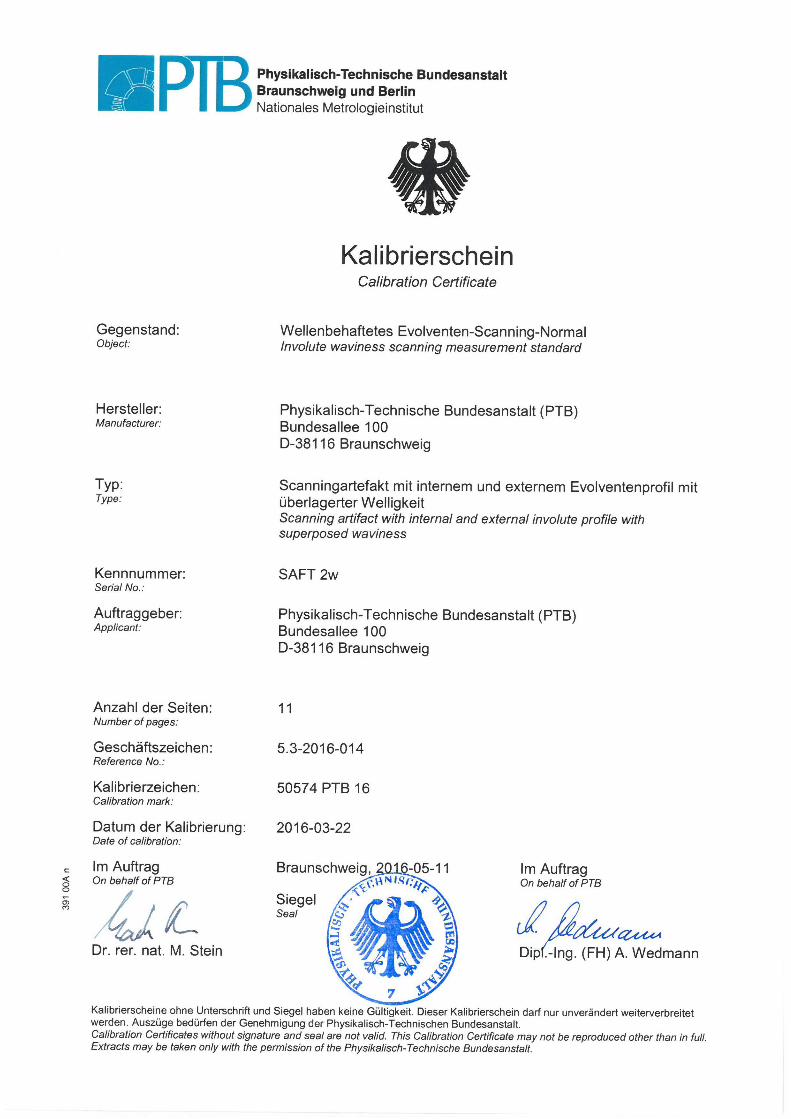
1) by PTB (see D2.1.1 and D2.1.2). In particular, for both profiles, the total deviation F, the

form deviation ff and the slope deviation fH have been calibrated; moreover, a spectral analysis has been performed using FFT method and the three main components of the spectrum have been calibrated in terms of wavelength and amplitude. Result are documented in PTB calibration certificate ref. n. 5.3-2016-014 (D2.1.2) INRIM investigated the influence of scanning parameter such as 5 different scanning speeds (from 2 mm/s to 24 mm/s), 3 different workpiece orientations inside the measurement \volume and 3 different stylus lengths (35 mm, 135 mm and 235 mm). Measurement result

have been analysed in order to evaluate, for both profiles, the deviations (F, ff and fH) according ISO 1328-1: 2013 and the influence due to the scanning measurement parameters on these result.

1. The measurement standard SAFT 2w the standard SAFT 2w is a plate with a diameter of 290 mm and a thickness of 20 mm, with 2 polished references on the border (a circle and a plan) in order to determine the reference axis of the workpiece (Fig. 1 and Fig. 2). The standard embodies an internal and an external involute profile both superposed with a certain waviness. The profiles have been manufactured with a wire-cut EDM machine. The machining data points have been obtained by using the function described in Figure 3. The three waviness parameters, which were used, are presented in the Table 1.

Geometry parameters

Outer diameter 290 mm

Face width 20 mm

Involute parameters:

Radius of base circle

Range of involute function inv(α) Int. involute: ------------------------ ext. Involute: -----------------------

20 mm 0°- 270° 0°- 200°

Nominal wavelength and amplitude:

------------------------------- -------------------------------- --------------------------------

8 mm; 5 μm 2.5 mm; 3 μm 0.8 mm; 1 μm

Tab. 1: Waviness parameters

Fig.1 SAFT 2W Artefact

Pag. 2 / 17

Fig. 2 Technical drawing of the internal involute waviness scanning measurement standard

Fig. 3: Parametric function and the sketch of the involute with waviness

Pag. 3 / 17

2. Experimental setup and plan of measurement Free form scanning on the SAFT 2w involute profiles was performed on a CMM Leitz PMM- C 12.10.7 with the following machine specification:

measuring volume: ;

EMPE = ; PFTU = ;

Resolution= ;

Stylus model: Leitz trax (tip diameter : 3 mm). One face of SAFT 2w was equipped with 4 PT100 probes for temperature compensation (Fig 4a). Measurement was performed, for both profiles (Fig. 4b), according the following scanning measuring parameters:

workpiece orientations (WO): 0°, 90° and 210° (Fig. 5);

scanning speed (SS): 2, 8, 14, 20, 24 mm/s;

stylus length (SL) : 35, 135 and 235 mm (135 mm and 235 mm have been obtained by means two titanium extensions of 100 mm and 200 mm, respectively);

3 scanning measure repetitions for each parameter set.

Fig 4: a) thermometers arrangement; b) example of internal involute measuring scanning

Fig 5: Workpiece orientations: 0°, 90° and 210° with respect to machine x-axis and y-axis (green)

Pag. 4 / 17

3. Scanning measurement result and data analysis According to scanning parameters, a total of 270 measurement profiles have been performed1. Measurement required two day of machine functioning during which temperature has ranged from 20.5 °C to 20.7 °C. The coordinate system taken for measuring was strictly in accordance with the artefact calibration certificate issued by PTB [2] (Fig 6). From the measurement data the profiles have been calculated as function of length of roll. Then, the theoretical involute was subtracted from data.

Fig. 6. Sketch of the SAFT w2 (by PTB report D.2.1.2)

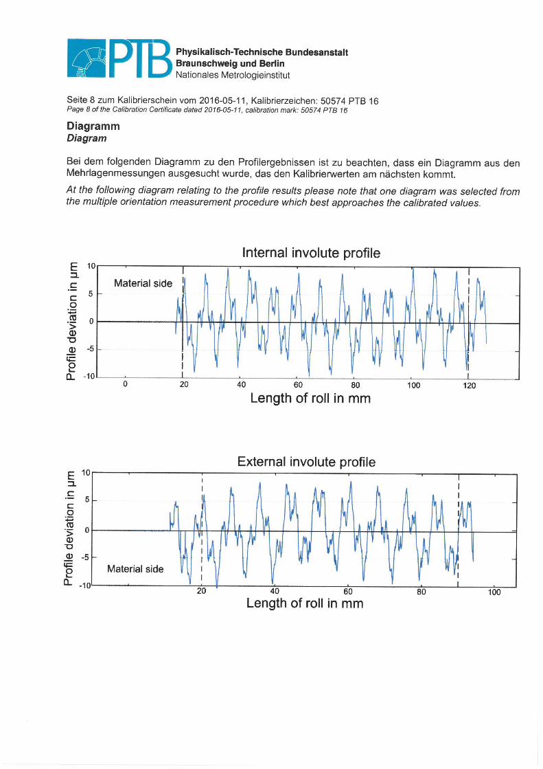
A first evaluation of computed data, evidenced the presence of an unexpected periodic deviation of the profile that seemed to reveal some eccentricity2. The reduction of eccentricity by theoretical correction gave as result a profile deviation behaviour very similar to the one showed in PTB certificate (see Fig. 7 and Fig 8)

Fig. 7. Example of internal involute profile By PTB certificate n. ref. n. 5.3-2016-014

1 For more details on measurement execution (Quindos part-program) see Annex A

2 The presence of periodic deviation has not been evidenced by SAFT 2w calibration certificate [2]- see Annex B .

Pag. 5 / 17

Fig. 8: Profile obtained by measurement without eccentricity reduction and profile reduced by an eccentricity ̅

Despite this positive result, the whole sinusoidal effect seems not to be removed by means of the reduction of a mean eccentricity (see Fig. 9 and Fig. 10), moreover correction induce irregularity in fHa values as function of workpiece orientations (see Tab. 2, 3, 4, and 5); this could suggest the

Pag. 6 / 17

presence of other effects, as for example thermal effects, that could contribute to the evidenced trend, but these further effects will not be investigated in the present draft. Notice that also the CMI institute (a project partner) during Final meeting declared that they found the same data behaviour during measurement and that they analysed the measurement data by correcting a theoretical eccentricity even if the correction procedure has not been cited (and therefore described) inside of their deliverable report. Considering only the presence of an eccentricity as influence effect, a reduction of data distribution has been necessary for the evaluation of profile deviations. In order to reduce eccentricity effects, a mean eccentricity on three couple of coordinates3 has been computed and then it has been

mathematically removed by all measured profiles.

Fig. 9: profile deviation before and after the introduction of a polar eccentricity e*; Internal involute profile

3

The mean eccentricity ̅ has been evaluated on 1 repetition and 3 workpiece orientations at scanning speed of 2 mm/s

and stylus length of 35 mm in the case of internal involute profile. See Annex C for more details

Pag. 7 / 17

Fig. 10: profile deviations before and after the introduction of a polar eccentricity e*; Internal involute profile

As previously evidenced, the mathematical correction, contributes to reduce the sinusoidal effect but it does not remove whole effect, especially in the case of external involute profile, that shows higher values of profile deviations with respect to internal one (see Tab. 2, 3, 4 and 5) Tab. 2 and Tab. 4 show the result of profile deviation analysis conducted on the data distributions

reduced by eccentricity. In particular, for both profiles, the total deviation F, the form deviation ff

and the slope deviation fH have been evaluated within the following evaluation ranges:

involute Length of roll

Internal involute 20 mm ÷ 120 mm

External involute 20 mm ÷ 90 mm

Tab. 3 and tab. 5 show the variability of profile deviations with respect to mean profile deviations evaluated at the best measurement conditions; they have been considered as best measurement conditions those conditions that would theoretically guaranteed the lowest effects on measurement result due to scanning speed and stylus length. Therefore, the mean profile deviations have been computed considering the profile deviation values at the following conditions: SL= 35 mm, SS= 2 m/s and WO= 0°, 90°, 210° because it was not possible to distinguish the best workpiece orientation a priori (see Annex C for more details about eccentricity correction). As example of uncorrected profile deviation, Tab. 6 shows the profile deviations for the internal involute profile without eccentricity correction whereas Tab. 7 shows the corrected sample standard deviations of deviation profiles by varying the scanning speed.

The total deviation F, the form deviation ff and the slope deviation fH in case of uncorrected

condition (values in Tab. 6) are also shown in Fig. 11, 12 and 13.

Pag. 8 / 17

Tab 2: internal involute profile deviations

Pag. 9 / 17

Tab. 3: Internal profile deviations variability with respect to mean profile deviations at best scanning conditions (SS= 2 mm/s, SL= 35 mm, for all orientations)

Pag. 10 / 17

Tab 4: External involute profile deviations

Pag. 11 / 17

Tab. 5: External profile deviations variability with respect to mean profile deviations evaluated at best scanning conditions

(SS= 2 mm/s, SL= 35 mm, for all orientations)

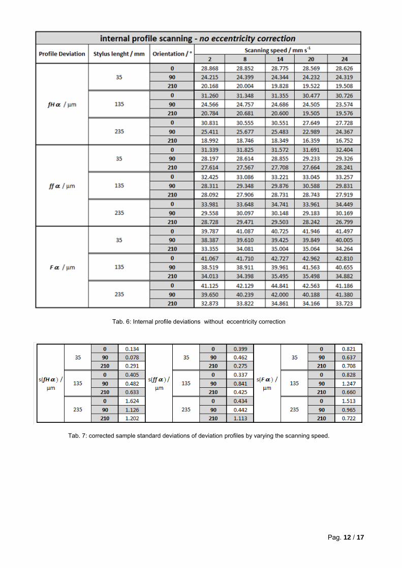
Pag. 12 / 17

Tab. 6: Internal profile deviations without eccentricity correction

Tab. 7: corrected sample standard deviations of deviation profiles by varying the scanning speed.

Pag. 13 / 17

Fig. 11: Total deviation at different scanning speeds, workpiece orientations and Stylus lengths – internal involute

Fig. 12: form deviation at different scanning speeds, workpiece orientations and Stylus lengths – internal involute

Pag. 14 / 17

Fig. 13: slope deviation at different scanning speeds, workpiece orientations and Stylus lengths – internal involute

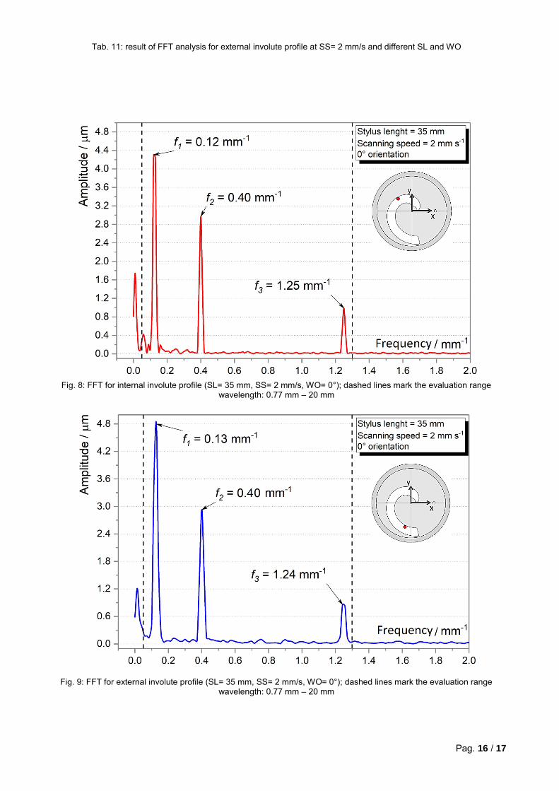
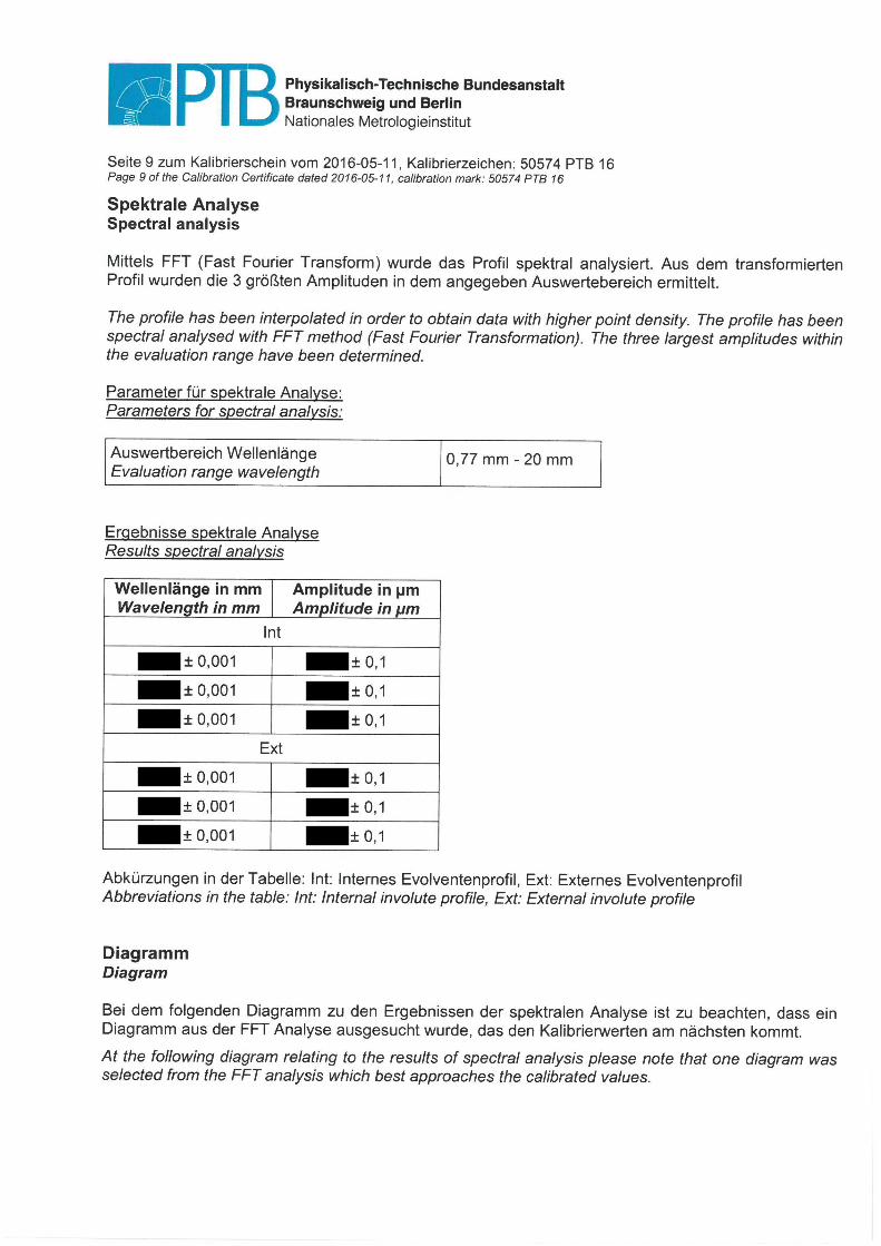
After the profile deviation analysis, measurement data have been spectral analysed by means of FFT method in order to determine the superimposed waviness as a function of scanning parameters; furthermore the three largest amplitudes within the evaluation range have been determined. The found wavelengths and amplitudes indicates the presence of a waviness consistent with the superposed nominal waviness (see section 1) . Tables 8, 9, 10 and 11 summarize result obtained at different measurement conditions (workpiece orientations, scanning speeds and stylus lengths). Since data analyses show that scanning conditions do not influence significantly the FFT result and that detection of superposed waviness is very repeatable with scanning speeds (SS) (see Tab 8 and Tab. 10), it has been decided to show the result at different stylus lengths (SL) and orientations (WO) only in the cases of SS= 2 mm/s. Finally, Fig. 14 and Fig. 15 show two examples of conduced FFT analysis.

SL= 35 mm, WO= 0° - INTERNAL INVOLUTE PROFILE

SS / mm s-1

f1 / mm-1

1 / mm A1 / m f2 / mm-1

2 / mm A2 / m f3 / mm-1

3 / mm A3 / m

2 0.1201 8.330 4.304 0.4002 2.499 2.970 1.2505 0.800 0.990

8 0.1200 8.331 4.298 0.4001 2.499 2.972 1.2503 0.800 1.089

14 0.1200 8.333 4.290 0.4001 2.500 3.005 1.2502 0.800 1.182

20 0.1200 8.332 4.321 0.4001 2.500 3.044 1.2502 0.800 1.051

24 0.1200 8.333 4.323 0.4000 2.500 3.094 1.2500 0.800 1.043

Tab. 8. result of FFT analysis for the internal involute profile at different SS and at SL= 35 mm, WO= 0°

Pag. 15 / 17

SS = 2 mm/s, WO= 0° - INTERNAL INVOLUTE PROFILE

SL / mm f1 / mm-1 1 / mm A1 / m f2 / mm-1 2 / mm A2 / m f3 / mm-1 3 / mm A3 / m

35 0.1201 8.330 4.304 0.4002 2.499 2.970 1.2505 0.800 0.990

135 0.1200 8.331 4.311 0.4001 2.499 2.975 1.2504 0.800 0.993

235 0.1200 8.331 4.318 0.4001 2.499 2.976 1.2504 0.800 1.002

SS = 2 mm/s, WO= 90°- INTERNAL INVOLUTE PROFILE

SL / mm f1 / mm-1 1 / mm A1 / m f2 / mm-1 2 / mm A2 / m f3 / mm-1 3 / mm A3 / m

35 0.1200 8.334 4.274 0.4000 2.500 2.969 1.2499 0.800 0.990

135 0.1201 8.330 4.293 0.4002 2.499 2.981 1.2505 0.800 0.996

235 0.1201 8.330 4.310 0.4002 2.499 2.983 1.2505 0.800 1.014

SS = 2 mm/s, WO= 210° - INTERNAL INVOLUTE PROFILE

SL / mm f1 / mm-1 1 / mm A1 / m f2 / mm-1 2 / mm A2 / m f3 / mm-1 3 / mm A3 / m

35 0.1200 8.333 4.313 0.4000 2.500 2.972 1.2501 0.800 0.991

135 0.1200 8.333 4.308 0.4000 2.500 2.972 1.2501 0.800 0.994

235 0.1200 8.333 4.323 0.4000 2.500 2.975 1.2500 0.800 0.993

Tab. 9: result of FFT analysis for internal involute profile at SS= 2 mm/s and different SL and WO

SL= 35mm, WO= 0° - EXTERNAL INVOLUTE PROFILE

SS / mm s-1 f1 / mm-1 1 / mm A1 / m f2 / mm-1 2 / mm A2 / m f3 / mm-1 3 / mm A3 / m

2 0.1286 7.777 4.799 0.4001 2.500 2.928 1.2430 0.804 0.857

8 0.1286 7.779 4.806 0.4000 2.500 2.935 1.2570 0.796 1.063

14 0.1286 7.776 4.799 0.4001 2.500 2.970 1.2574 0.795 0.993

20 0.1286 7.776 4.767 0.4001 2.499 3.069 1.2432 0.804 0.890

24 0.1286 7.777 4.779 0.4001 2.500 3.142 1.2430 0.804 0.873

Tab. 10. result of FFT analysis for the external involute profile at different SS and at SL= 35 mm, WO= 0°

SS = 2 mm/s, WO= 0°- EXTERNAL INVOLUTE PROFILE

SL / mm f1 / mm-1 1 / mm A1 / m f2 / mm-1 2 / mm A2 / m f3 / mm-1 3 / mm A3 / m

35 0.1286 7.777 4.799 0.4001 2.500 2.928 1.2430 0.804 0.857

135 0.1286 7.777 4.799 0.4001 2.500 2.936 1.2430 0.804 0.871

235 0.1286 7.777 4.806 0.4001 2.500 2.932 1.2430 0.804 0.880

SS = 2 mm/s, WO= 90°- EXTERNAL INVOLUTE PROFILE

SL / mm f1 / mm-1 1 / mm A1 / m f2 / mm-1 2 / mm A2 / m f3 / mm-1 3 / mm A3 / m

35 0.1286 7.775 4.781 0.4001 2.499 2.927 1.2432 0.804 0.865

135 0.1286 7.776 4.770 0.4001 2.499 2.935 1.2432 0.804 0.873

235 0.1286 7.776 4.770 0.4001 2.499 2.938 1.2431 0.804 0.915

SS = 2 mm/s, WO= 210°- EXTERNAL INVOLUTE PROFILE

SL / mm f1 / mm-1 1 / mm A1 / m f2 / mm-1 2 / mm A2 / m f3 / mm-1 3 / mm A3 / m

35 0.1286 7.778 4.793 0.4000 2.500 2.934 1.2428 0.805 0.860

135 0.1286 7.776 4.782 0.4001 2.500 2.930 1.2431 0.804 0.862

235 0.1286 7.776 4.772 0.4001 2.500 2.924 1.2431 0.804 0.891

Pag. 16 / 17

Tab. 11: result of FFT analysis for external involute profile at SS= 2 mm/s and different SL and WO

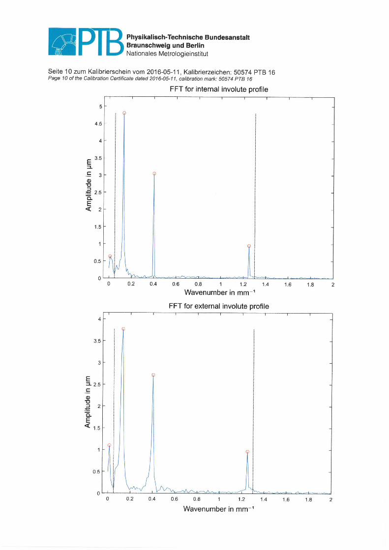
Fig. 8: FFT for internal involute profile (SL= 35 mm, SS= 2 mm/s, WO= 0°); dashed lines mark the evaluation range

wavelength: 0.77 mm – 20 mm

Fig. 9: FFT for external involute profile (SL= 35 mm, SS= 2 mm/s, WO= 0°); dashed lines mark the evaluation range wavelength: 0.77 mm – 20 mm

Pag. 17 / 17

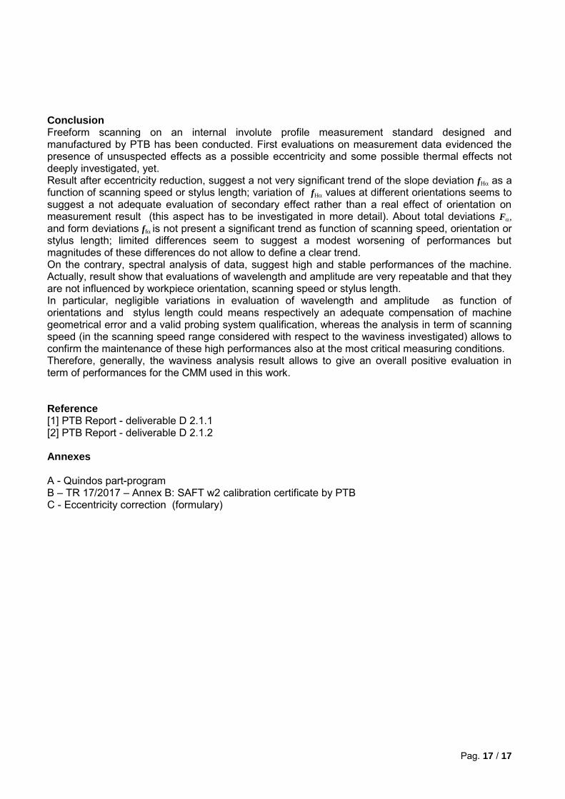
Conclusion Freeform scanning on an internal involute profile measurement standard designed and manufactured by PTB has been conducted. First evaluations on measurement data evidenced the presence of unsuspected effects as a possible eccentricity and some possible thermal effects not deeply investigated, yet. Result after eccentricity reduction, suggest a not very significant trend of the slope deviation fH as a function of scanning speed or stylus length; variation of fH values at different orientations seems to suggest a not adequate evaluation of secondary effect rather than a real effect of orientation on measurement result (this aspect has to be investigated in more detail). About total deviations F,

and form deviations ffis not present a significant trend as function of scanning speed, orientation or stylus length; limited differences seem to suggest a modest worsening of performances but magnitudes of these differences do not allow to define a clear trend. On the contrary, spectral analysis of data, suggest high and stable performances of the machine. Actually, result show that evaluations of wavelength and amplitude are very repeatable and that they are not influenced by workpiece orientation, scanning speed or stylus length. In particular, negligible variations in evaluation of wavelength and amplitude as function of orientations and stylus length could means respectively an adequate compensation of machine geometrical error and a valid probing system qualification, whereas the analysis in term of scanning speed (in the scanning speed range considered with respect to the waviness investigated) allows to confirm the maintenance of these high performances also at the most critical measuring conditions. Therefore, generally, the waviness analysis result allows to give an overall positive evaluation in term of performances for the CMM used in this work. Reference [1] PTB Report - deliverable D 2.1.1 [2] PTB Report - deliverable D 2.1.2 Annexes A - Quindos part-program B – TR 17/2017 – Annex B: SAFT w2 calibration certificate by PTB C - Eccentricity correction (formulary)

Annex A - T.R. 17/2017: Q7 part program “DriveTrain evolvente.wdb” – 01/08/2017 for the scanning of the internal involute waviness standard performed on the INRIM CMM Leitz PMM- C 12.10.7 ! ------------------------- JRP DriveTrain --------------------------- !---------------------- Campione d'evolvente ------------------------- ! Geometria del campione !distanza dal bordo esterno del colletto per la presa punti del piano superiore BORDO=5 SEMI_SPESSORE=10 SEMI_INGOMBRO=145 ~TEMPER_FILE=C:\002 - Corradi NI\filePerQ7.txt ~RADICE_FILE=C:\Users\LNPC775\Desktop\DriveTrain evolvente\MISURE\Pos0210-St235-Vel ~RIPETIZIONE=-Rip3.txt SPEED(1)=2 SPEED(2)=8 SPEED(3)=14 SPEED(4)=20 SPEED(5)=24 ! Velocità !USECMM (NAM=LENTA) USECMM (NAM=VELOCE) ! Qualifica tastatore DfnArtefact (NAM=S1, DIA=CAL$NOR, SAZ=0.0, SEL=90.0, SDM=8.0, COE=0.0000065) QualifyTool (NAM=PRB, DIA=3.000, NRF=Y, REF=S1, SCN=Y, SNT=TRX, RPT=(0,0,-235), DEL=N, GEO=SPH) MoveCmmInmm (TYP=DLT, DST=(,,100)) SHOW (NAM=PRB, DEV=TT, TYP=ELE, STY=EVA) STOP MessageBox (STR="Misura manuale?", BUT=4, ICO=2, DFB=1) If (BXP=~MsgBoxResult=="Yes") ! Sistema di riferimento manuale EDTMSG (NAM=PIANO_MAN, CRE=Y) MEPLA (NAM=PIANO_MAN, CSY=CMMA$CSY, ITY=GSS, MSG=PIANO_MAN, DEL=Y) EDTMSG (NAM=CENTRO_MAN, CRE=Y) MECIR (NAM=CENTRO_MAN, CSY=CMMA$CSY, PRO=PIANO_MAN, PTY=EX, MSG=CENTRO_MAN, DEL=Y) EDTMSG (NAM=CERCHIO_MAN, CRE=Y) MECIR (NAM=CERCHIO_MAN, CSY=CMMA$CSY, PRO=PIANO_MAN, PTY=EX, MSG=CERCHIO_MAN, DEL=Y) DIPNTPNT (NAM=ASSE_X_MAN, CSY=CMMA$CSY, EL1=CENTRO_MAN, EL2=CERCHIO_MAN) BLDCSY (NAM=CSY_MAN, TYP=CAR, SPA=PIANO_MAN, SDR=+Z, PLA=ASSE_X_MAN, PDR=+X, XZE=CENTRO_MAN, YZE=CENTRO_MAN, ZZE=CENTRO_MAN) EndIf USECSY (NAM=CSY_MAN) ! Ripresa sistema di riferimento automatico GENCIR (NAM=PIANO_AUT, XCO=0, YCO=0, ZCO=0, DIA=CENTRO_MAN.$A-2*BORDO, NPT=8, PLA=XY, INO=P, CSY=CSY_MAN, ZVL=50) GENCIR (NAM=CENTRO_AUT, XCO=0, YCO=0, ZCO=-SEMI_SPESSORE, DIA=CENTRO_MAN.$A, NPT=8, PLA=XY, INO=O, CSY=CSY_MAN, ZVL=50+SEMI_SPESSORE) GENCIR (NAM=CERCHIO_AUT, XCO=ASSE_X_MAN.$A, YCO=0, ZCO=-SEMI_SPESSORE, DIA=CERCHIO_MAN.$A, NPT=8, PLA=XY, INO=I, CSY=CSY_MAN, ZVL=50+SEMI_SPESSORE) MoveCmmInmm (TYP=ABS, DST=(0,0,100), CSY=CSY_MAN) MEPLA (NAM=PIANO_AUT, CSY=CSY_MAN, ITY=GSS) MECIR (NAM=CENTRO_AUT, CSY=CSY_MAN, PRO=PIANO_AUT, PTY=EX) MECIR (NAM=CERCHIO_AUT, CSY=CSY_MAN, PRO=PIANO_AUT, PTY=EX) DIPNTPNT (NAM=ASSE_X_AUT, CSY=CSY_MAN, EL1=CENTRO_AUT, EL2=CERCHIO_AUT) BLDCSY (NAM=CSY_AUT, TYP=CAR, SPA=PIANO_AUT, SDR=+Z, PLA=ASSE_X_AUT, PDR=+X, XZE=CENTRO_AUT, YZE=CENTRO_AUT, ZZE=CENTRO_AUT) !----------------------------------- ! !---------- TEMPERATURE------------- ! !------------------------------------! ! acquisizione Temperature scale CMM ! ! LEGGO SOLO TMPCOMP (COE=0.000000, AUT=Y, TEL=TEMP, DEL=Y) ! GETVALS (OBJ=TEMP, TYP=ELE, RDS=(X,Y,Z), REA=(X,Y,Z)) ! acquisizione Temperature campione evolvente ! chiama la procedura DELCHS (NAM=CHS:~IMP2EVA_*, CNF=N, TYP=CHS) ~IMP2EVA_FILE = ~TEMPER_FILE ~IMP2EVA_X = 'TERM_1' ~IMP2EVA_Y = 'TERM_2' ~IMP2EVA_Z = 'TERM_3' ~IMP2EVA_A = 'TERM_4' ~IMP2EVA_B = '' ~IMP2EVA_D = ''

~IMP2EVA_E = '' ~IMP2EVA_F = '' INDPRC (NAM=IMP2EVA) ! copia elemento creato dalla procedura e poi lo cancella CPYOBJ (FRM=IMP2EVA_ELE, TO =TEMP_CAL_A) DELELE (NAM=IMP2EVA_ELE, CNF=N) !leggo le 4 temperature GETVALS (OBJ=TEMP_CAL_A, TYP=ELE, RDS=(X,Y,Z,A), REA=(T1,T2,T3,T4)) MEDIAT=(T1+T2+T3+T4)/4 TMPCOMP (TEX=X, TEY=Y, TEZ=Z, TEW=MEDIAT, COE=0.0000115, AUT=N, TEL=TEMP_CAL_A, DEL=N) DO (NAM=I, BGN=1, END=5) ! muove in posizione inizio scansione interno MoveCmmInmm (TYP=ABS, DST=(16,26,20), CSY=CSY_AUT) !Imposta la velocià di scansione PUTVALS (OBJ=CONTORNO_INT.NOM.PTS(3), TYP=ELE, RDS=A, VAL=SPEED(I)) !scansione bordo interno ME2DE (NAM=CONTORNO_INT, CSY=CSY_AUT, INO=O) !compone stringa per output ~VEL=-Int CVREACHS (NAM=~VELOCITA, VAL=SPEED(I), FM1=2, INT=Y, ANG=N, SPZ=Y, RLS=Y, RTZ=Y) CONCAT (NAM=~PERCORSO, STR=(~RADICE_FILE,~VELOCITA,~VEL,~RIPETIZIONE), INI=Y) !esporta la scansione FMTOBJ (FIL=~PERCORSO, NAM=CONTORNO_INT, STA=NEW, TYP=ELE, STY=APT, DSC=(X,Y,Z), DEL=Y) ! muove in posizione MoveCmmInmm (TYP=ABS, DST=(17,-112,20), CSY=CSY_AUT) MoveCmmInmm (TYP=ABS, DST=(16,26,20), CSY=CSY_AUT) !imposta velocità di scansione PUTVALS (OBJ=CONTORNO_EST.NOM.PTS(3), TYP=ELE, RDS=A, VAL=SPEED(I)) !scansione bordo esterno ME2DE (NAM=CONTORNO_EST, CSY=CSY_AUT) !compone stringa per output ~VEL=-Est CVREACHS (NAM=~VELOCITA, VAL=SPEED(I), FM1=2, INT=Y, ANG=N, SPZ=Y, RLS=Y, RTZ=Y) CONCAT (NAM=~PERCORSO, STR=(~RADICE_FILE,~VELOCITA,~VEL,~RIPETIZIONE), INI=Y) !esporta la scansione FMTOBJ (FIL=~PERCORSO, NAM=CONTORNO_EST, STA=NEW, TYP=ELE, STY=APT, DSC=(X,Y,Z), DEL=Y) MoveCmmInmm (TYP=ABS, DST=(17,-112,20), CSY=CSY_AUT) MoveCmmInmm (TYP=ABS, DST=(16,26,20), CSY=CSY_AUT) ENDDO !----------------------------------- ! !---------- TEMPERATURE-R----------- ! !------------------------------------! ! acquisizione Temperature campione evolvente ! chiama la procedura DELCHS (NAM=CHS:~IMP2EVA_*, CNF=N, TYP=CHS) ~IMP2EVA_FILE = ~TEMPER_FILE ~IMP2EVA_X = 'TERM_1' ~IMP2EVA_Y = 'TERM_2' ~IMP2EVA_Z = 'TERM_3' ~IMP2EVA_A = 'TERM_4' ~IMP2EVA_B = '' ~IMP2EVA_D = '' ~IMP2EVA_E = '' ~IMP2EVA_F = '' INDPRC (NAM=IMP2EVA) ! copia elemento creato dalla procedura e poi lo cancella CPYOBJ (FRM=IMP2EVA_ELE, TO =TEMP_CAL_R) DELELE (NAM=IMP2EVA_ELE, CNF=N) ! ----------- ! ! Report ! ! ----------- ! ! si riportano i due elementi sottostamti secondo il CMMA$CSY TRAELE (NEW=CENTRO_ASSOLUTO, TRA=CMMA$CSY, OLD=CENTRO_AUT, TYP=CSY, RPL=Y, EVA=N) TRAELE (NEW=ASSE_X_ASSOLUTO, TRA=CMMA$CSY, OLD=ASSE_X_AUT, TYP=CSY, RPL=Y, EVA=N) DELQUE (NAM=$RPO, CNF=N, TYP=QUE) ADDEVA (NAM=(PRB,TEMP_CAL_A,TEMP_CAL_R)) ADDEVA (NAM=(CENTRO_ASSOLUTO,ASSE_X_ASSOLUTO)) FLEXREPORT (LAY=VICI, PRI=N, XFL=C:\Users\LNPC775\Desktop\DriveTrain evolvente\MISURE\report) STOP

Annex C - T.R. 17/2017: Eccentricity correction and calculation of the profile deviation parameters ( , and ) of the standard involutes (SAFT 2W): procedure and formulary

The procedure is synthetically articulated in the following steps:

1. Determination of the components of the polar eccentricity vector ̅ by means of the

Microsoft Excel built-in optimization tool “Solver” in the best scanning conditions (v = 2 mm

s-1, stylus length = 35 mm), averaging the obtained values among the 3 different workpiece

orientation (0°, 90° and 210°).

2. Creation of an OriginLab Origin batch working on the suitable roll length ranges for both

external and internal involute profiles to generate, for all the scanning conditions

(combinations of 5 variable speeds, 3 stylus lengths and 3 workpiece orientations), the

following ordered quantities:

a. the eccentric coordinates and of an arbitrary point on the involute profile

by correction of the the CMM acquired points with the previously calculated ̅

components (ex and ey);

b. the module of the position vector of the same point: √

;

c. the “eccentric” anomaly: (

) ;

d. the roll angle: (

) , where Rb = base radius;

e. the “observed” roll length: √

(being Rp = radius of the probe

tip, the “+” sign for the internal involute profile and the “–“ sign for the external

involute profile);

f. the “expected” roll lenght: ;

g. the difference between the observed and the expected roll length, that is the profile

deviation .

3. Performance of linear regressions on the vectors of data, so that the obtained slopes

define the parameter. The other profile parameters are calculated in the following way:

being residuals = difference between regression line and profile deviation for each

experimental point, ( ) ( ); ( ) ( ) .

Rb

𝜃

l

P

Involute profile