a pipelined adaptive lattice filter architecture - parhi

IEEE TRANSACTIONS ON SIGNAL PROCESSING, VOL. 41, NO. 5 , MAY 1993 I925

A Pipelined Adaptive Lattice Filter Architecture Naresh R. Shanbhag, Student Member, IEEE, and Keshab K. Parhi, Senior Member, IEEE

Abstract-The stochastic gradient adaptive lattice filter is pipelined by the application of relaxed look-ahead. This form of look-ahead maintains the functional behavior of the algorithm instead of the input-output mapping and is suitable for pipelining adaptive filters. The sum and product relaxations are employed to pipeline the adaptive lattice filter. The hardware complexity of the proposed pipelined adaptive lattice filters is the same as for the sequential filter, and is independent of the level of pipelining or speedup. Thus, the new architectures are very attractive in terms of implementation. Two pipelined architectures along with their convergence analyses are presented to illustrate the tradeoff offered by relaxed look-ahead. Simu- lation results supporting the conclusions of the convergence analysis are provided. The proposed architectures are then employed to develop a pipelined adaptive differential pulse-code modulation codec for video compression applications. Speedup factors up to 20 are demonstrated via simulations with image data.

I. INTRODUCTION HE design of concurrent signal processing algorithms T for real-time applications requiring high speed is cur-

rently of interest. To this end, algorithm transformation techniques [ 11 have formalized the methodology for ex- ploiting concurrency hidden in conventional digital signal processing algorithms. Of the two approaches for achieving high speed, pipelining [2] and parallel processing [3], the former is attractive due to its reduced hardware requirements.

The look-ahead pipelining [2] demonstrated the feasi- bility of high-speed implementation of signal processing algorithms. However, this technique achieves high speed by creating additional concurrency in nonconcurrent signal processing algorithms, at the expense of significant hardware overhead. Even though the look-ahead pipelining technique has been successfully applied to numerous problems [2], [4]-[7], its extremely high hardware complexity makes it difficult to implement. This problem is compounded further if pipelining of adaptive filters is at- tempted [8], [9]. Therefore, an alternative to algorithm transformation techniques [ 11 is to develop inherently pipelinable digital signal processing algorithms. Further- more, the hardware requirements of these pipelinable algorithms and the traditional nonconcurrent algorithms should be the same or similar.

Manuscript received October 11, 1991; revised June 4 , 1992. The associate editor coordinating the review of this paper and approving it for publication was Prof. Ed F. Deprettere. This work was supported by the A m y Research Office under Contract DAAL-90-G-0063.

The authors are with the Department of Electrical Engineering, Univer- sity of Minnesota, Minneapolis, MN 55455.

IEEE Log Number 9207529.

In this paper, we present an approximate form of look- ahead referred to as relaxed look-ahead [ 101. The conventional look-ahead technique [2] transforms a given serial algorithm into an equivalent (in the sense of input-output mapping) pipelined one. The relaxed look-ahead sacri- fices this equivalence between the serial and pipelined algorithms at the expense of marginally altered convergence characteristics. Therefore, the relaxed look-ahead maintains the functionality of the algorithm and is well suited for adaptive filtering applications. However, unlike look-ahead, application of relaxed look-ahead requires a subsequent convergence analysis of the resulting pipelined algorithm.

The relaxed look-ahead is employed to design new concurrent stochastic gradient lattice adaptive algorithms [ 111, which are inherently pipelined. The adaptive lattice filters designed using relaxed look-ahead have the property that the hardware requirements for these filters are independent of the speedup or the level of pipelining. In contrast, the hardware requirements in look-ahead increase with the speedup (although logarithmically). The proposed adaptive lattice algorithms are then employed to develop a pipelined adaptive pulse-code-modulation (ADPCM) codec for image compression applications. Preliminary results on the performance of the pipelined ADPCM codec were found to be very promising [ 121. As expected, the hardware requirements for the new ADPCM codec was found to be independent of the number of quantizer levels L, the order of the predictor N, and the speedup M. This is in contrast to the pipelined codec architecture developed via look-ahead in [5]. The application of look-ahead in [5] proceeded in two steps. First, the ADPCM loop was linearized by moving the quantizer outside. This step resulted in an increase in the hardware complexity of O(L). Then, the look-ahead was applied to the linearized loop. This two-step process resulted in a hardware complexity which is strongly dependent on L, N, and M. The architecture in [5] was for a ADPCM codec with a transversal predictor and therefore a comparison with lattice ADPCM codec may seem unfair. How- ever, similar conclusions were reached in [ 131, where a pipelined transversal ADPCM codec was developed via relaxed look-ahead. An additional advantage of the proposed codec is the fact that the output latency is usually much smaller than the level of pipelining.

In addition to the transversal ADPCM codec [13], the relaxed look-ahead has also been successfully applied to pipeline the transversal LMS algorithm [ lo] . The hardware increase in the pipelined architecture was only the

1053-587X/93$03.00 0 1993 IEEE

1926 IEEE TRANSACTIONS ON SIGNAL PROCESSING, VOL. 41, NO. 5 , MAY 1993

pipelining latches. This is a remarkable improvement over previous attempts at high-speed adaptive filtering [ 141-

We first explain the technique of pipelining in Section I1 and then describe the relaxed look-ahead in Section 111. In Section IV, we develop two pipelined stochastic gradient lattice filter architectures PIPSGLAl and PIPSGLA2 and compare the hardware requirements of the serial architecture (SSGLA) [ 113 and the architecture resulting from the conventional deterministic look-ahead (DLAS- GLA) [8]. The results of the convergence analysis of PIPSGLAl and PIPSGLA2 are presented in Section V. The pipelined ADPCM codec is developed in Section VI. The simulation results presented in Section VI1 confirm the results of our analysis and demonstrate the performance of the pipelined codec.

1171.

11. PIPELINING Conventionally, pipelining has been viewed as an ar-

chitectural technique for increasing the throughput of an algorithm. However, in [18] the use of pipelining for reducing power consumption in VLSI chips has been described. This fact extends the utility of pipelined algorithms from high-speed (high-power) applications such as video compression to low-speed (low-plower) applications such as speech compression.

A. A High Throughput Technique Consider an algorithm (see Fig. l(a)) consisting of two

computational blocks A and B . The throughput of this serial (or unpipelined) system is limited by

1 funp ipe 5 ~ (2.1)

TA -k TB

where TA and Ts are the computation times of blocks A and 'B, respectively.

In order to increase the throughput, we need to pipeline the system in Fig. l(a) by introducing pipelining latches. A two-stage pipelined system is shown in Fig. l(b). The throughput of this pipelined system is

which is clearly greater than that of the serial system in Fig. l(a). This increase in throughput has been made at the expense of an increase in the output latency. For the serial system, the output corresponding to the current input is generated in the current clock cycle. However, for the pipelined system, the output is delayed by one clock cycle. In general, assuming that each stage has the same delay, the throughput of a system pipelined by M stages is M times that of the serial system, while its output latency increases by the computational delay associated with the M pipelining latches.

B. A Low Power Technique We now show how pipelining can be employed to de-

sign low-power circuits. The dynamic power consump-

nn

Fig. 1 . Pipelining: (a) a serial system, and (b) equivalent pipelined system.

tion ( P ) of a CMOS circuit is given by

(2.3)

where Ctotal is the total switching capacitance, Vdd is the supply voltage and f is the clock frequency. From (2.3) it is clear that dramatic reductions in power are possible by reducing the supply voltage for a constant clock frequency.

Consider the serial algorithm of Fig. l(a). The propagation delay at supply voltage of Vdd (tpd,unpipe ( Vdd)) of the serial algorithm is given by

where CL is the capacitance along the critical path in Fig. l(a), V, is the device threshold voltage, and E is a constant which depends on the process parameters. In an optimally designed system the propagation delay should in fact equal the clock period.

For a M-stage pipelined system, the propagation delay tpd,pipe ( Vdd) is

which is M times less than that of the serial algorithm. Clearly, the pipelined system can be clocked at a much higher frequency than is necessary. However, by reducing Vdd, we can increase the propagation delay of the pipelined system till it equals that of the serial system. This step not only matches the propagation delay to the desired clock period but also results in a reduction of power consumption.

There is however a lower limit to which the supply voltage can be reduced for a given value of VI. Let K1 be the factor by which the supply voltage of the pipelined system needs to be reduced for its propagation delay to equal that of the serial system. Equating tpd,pipe ( Vdd/K1) (from (2.5)) to tpd,unpipe(Vdd) (2.4) we get the following equation:

MV: K : - (2MVdd V, + (Vdd - V , ) 2, KI + MVid = 0

(2.6) which can be solved for K 1 given the pipelining level M. Substituting Vdd = 5 V and V, = 0.7 V, we find that for a two-stage pipelined system (i.e., M = 2) a supply voltage of 3.08 V is necessary for the two propagation delays

SHANBHAG AND PARHI: PIPELINED ADAPTIVE LATTICE FILTER 1927

to equal each other. At this supply voltage the power dissipation is reduced by a factor of 2.62. Similarly, for M = 3, a supply voltage of 2.43 V would be needed and the power dissipation would be reduced by a factor of 4 .

This analysis indicates that pipelining by fewer levels results in reduction of power dissipation at the same speed.

111. PIPELINING USING RELAXED LOOK-AHEAD In this section, we develop the relaxed look-ahead and

point out its significance in the development of inherently concurrent adaptive algorithms. First, we apply the look- ahead to a first order recursive section and then introduce the relaxed look-ahead.

Consider the first-order recursion given by

x(n + 1) = ax(n) + u(n). (3.1)

We first apply an M-step look-ahead to (3.1), which is equivalent to expressing x(n + M) in terms of x ( n ) . This leads to

M - I

x ( n + M ) = aMx(n> + C alu(n + M - 1 - i ) . i = O

(3.2)

The M - 1 extra latches introduced into the recursive loop by this transformation can be used to pipeline the multiply and add operations in the loop. Note that the second term in (3.2) is an additional overhead due to look-ahead and is called the look-ahead overheadf,(M). The argument of f , (M) indicates its dependence on the level of pipelining ( M ) .

The overhead in look-ahead is very hardware expensive and at times is impractical to implement. However, under certain circumstances we can substitute approximate expressions on the right-hand side (RHS) of (3.2). De- pending on the application at hand, different types of approximations (or relaxations) may be employed. We now formulate two such relaxations which are called the sum and the product relaxations. These two relaxations would be employed to pipeline the stochastic gradient lattice filter [ l l ] in the next section.

A. Sum Relaxation In (3.2), if a = 1 and the input u(n) remains more or

less constant over M cycles, then we can replace the summation inf,(M) with Mu@). The resulting expression is given by

B. Product Relaxation If a in (3.2) is time varying (i.e., we have a (n) instead

of a), but the magnitude of a (n) is close to unity, then we can replace a(n) by (1 - a’ (n)), where a’ (n) is close to zero. Then, (3.2) is approximated as

x ( n + M) = (1 - Ma’(n) )x (n) M - 1

+ C a‘u(n + M - 1 - i ) . (3.5)

Hence, (3.5) is the outcome of an application of a M-step relaxed look-ahead with product relaxation to (3.1).

These relaxations (and any other) constitute the relaxed look-ahead. The relaxations may be applied individually or in combination. As an example, the application of a M- step relaxed look-ahead with sum relaxation of (3.3) and product relaxation to (3. l ) , with time-varying coefficients, results in

i = O

x ( n + M) = (1 - MU’ (n))x(n) + MU(^). (3.6)

Thus, the relaxed look-ahead does not result in a unique final architecture. This is in contrast to look-ahead, where there is a one-to-one mapping between the resulting pipelined architecture and the original one. The mapping for relaxed look-ahead, on the other hand, is one to many. This point will be illustrated further when we develop two pipelined architectures for the stochastic gradient adaptive lattice filter.

The relaxed look-ahead is not an algorithm transformation technique in the conventional sense [ l ] . This is because it modifies the input-output behavior of the original algorithm. It may be called a transformation technique in a stochastic sense if the average output profile is maintained. This, however, depends upon the nature of the approximations made. The pipelined architecture resulting from the application of relaxed look-ahead can al- ways be clocked at a higher speed than the original one.

IV. PIPELINED ADAPTIVE LATTICE ARCHITECTURES The relaxed look-ahead, described in the previous sec-

tion, is employed in this section to develop inherently pipelined adaptive lattice filter architectures. Even though numerous adaptive lattice algorithms exist [ 1 1 1 , we choose a simple version of the stochastic-gradient lattice algorithm. It must be pointed out that the relaxed look-ahead can be used to pipeline any of the other adaptive lattice algorithms. The convergence analysis would, however, differ.

x ( n + M ) = aMx(n) + Mu(n). (3.3) A. The Serial Stochastic-Gradient Lattice Architecture We choose the stochastic-gradient lattice algorithm [ 1 11 The aM term in (3.3) can be precomputed if a is a con-

stant. If u(n) is close to 0, then another relaxation of (3.3) described by the following equations:

Thus, (3.3) and (3.4) are the results of application of M- step relaxed look-ahead with sum relaxations to (3.1).


c(nlm)

Fig. 2. The SSGLA architecture.

(4.3)

ef(nlm) = ef(nlm - 1)

- k,(n)eb(n - l ( m - 1) (4.4a)

eb(nlm) = eb(n - llm - 1)

- km(n)ef(nlm - 1) (4.4b)

where n denotes the time instance, m = 1, - - , N denotes the lattice stage number (N being the total number of stages or the order of the filter). Equations (4.1)-(4.3) and (4 .4) are referred to as the adaptation and order-update equations, respectively. The reflection coefficient k,,, (n) is updated according to (4.1). The energy S (n I m - 1) of the input signals e f (n (m - 1) and eb(n - l l m - 1) to the mth stage is recursively computed by (4.2). This energy is required to compute the normalized adaptation coefficient 0, (n). This serial stochastic-gradient lattice algorithm is referred to as the SSGLA algorithm.

The SSGLA is shown in Fig. 2, where the intermediate output c ( n ( m ) would be employed later (see section VI) to develop a pipelined ADPCM codec. The computation time T, of the critical path is equal to

T, = 4T, + ( N + 2)Tu (4.5) where T, and Tu are the computation times of a two-operand multiplier and adder, respectively. For simplicity,

we assume that squaring and the division operations take the same amount of time as multiplication, although in practice division operations may require longer computation time. In addition, we see that there are two recursive loops with computation times:

It is now desired to pipeline the SSGLA such that the clock period (T,) of the pipelined architecture (to be referred to as PIPSGLA) is less than T , / M , where M is the desired speedup. If Tp is greater than T,, then the recursive loops need not be pipelined. For this case, the speedup can be achieved by employing interstage pipelining only.

B. The Pipelined Stochastic-Gradient Lattice Architecture (PIPGLA)

The pipelining of SSGLA proceeds in two steps. First, we include the interstage pipelining of the SSGLA. If the desired speedup cannot be achieved with this level of pipelining, then finer grain loop pipelining with relaxed look-ahead is adopted. Interstage pipelining is trivial as the stages are connected in a non-recursive fashion. Let Ms and ML denote the number of interstage and loop pipelining latches, respectively. We can now apply relaxed look-ahead to pipeline the two recursive loops in SSGLA (Fig. 2).

We first apply a M,-step relaxed look-ahead with sum relaxation of (3.4) to (4.2), which describes the recursive computation of the input power. Like (3. l), (4.2) is a first- order recursion. Therefore, by inspection of ( 3 . 4 ) , the final result of the application of the sum relaxation to (4.2)

SHANBHAG AND PARHI: PIPELINED ADAPTIVE LATTICE FILTER

is given by

As the constant (1 - /3)ML can be precomputed, it is not necessary to apply the product relaxation.

Similarly, the application of a ML-step relaxed look- ahead with sum relaxation of (3.3) to (4.1) results in the following equation:

Note that the bracketed part of the first term in (4.8) represents a hardware module whose output equals its input raised to the power ML. It is possible to reduce the hardware complexity of this module via decomposition. How- ever, it is more efficient to apply the product relaxation. Before doing so, we need to confirm that the bracketed part of the first term in (4.8) is close to unity. This is shown next.

Taking the expectation of (4.7) in the limit as n + 00,

we get

= 1 - (1 - (4.9)

If is sufficiently small as compared to 1, then the left- hand side (LHS) of (4.9) is also very small as compared to unity. From (4.3), we see that

~

S(nlm - 1)

= &(n)(ej(nlm - 1) + e i ( n - llm - 1)). (4.10)

Comparing (4.10) and (4.9), we conclude that the bracketed term in (4.8) is indeed close unity. Thus, applying the product relaxation to (4.8) (see (3.5)), we get

km(n + M L ) = [ I - MLPm(n)<ej<n(m - 1)

+ e i ( n - 11m - l))lkm(n)

+ 2MLPm(n)ef(n(m - 1)

- eb(n - I (m - 1). (4.11)

Assuming that the inputs to an mth lattice stage are ef(n Im - 1) and eb(nlm - l ) , the following set of equations

i929

PIPSGLA architecture, referred to as PIPSGLA1 :

k,(n - Ms + ML)

= [ I - M ~ P ~ ( ~ - Ms)(e j (n - ~ ~ l m - 1)

+ e i ( n - Ms - 1 J m - l))]k,(n - Ms)

+ 2MLPm(n - Ms)ef(n - Mslm - 1)

~

completely describe the functional behavior of the first

(4.14)

ef(n - Ms(m) = ef(n - Mslm - 1)

- km(n)eb(n - Ms - l lm - 1)

(4.15a)

eb(n - Mslm) = eb(n - Ms - l lm - 1)

- km(n)ef(n - Mslm - 1). (4.15b)

The complete PIPSGLAI is shown in Fig. 3, where we see that the increase in the hardware complexity equals two multipliers and 2(ML - 1) + 2Ms latches for each stage. This is a remarkably low increase considering the available alternative architectures [8], [9].

An alternative pipelined architecture PIPSGLA2 can be obtained by simply introducing ML latches into the recursive loops in Fig. 2. This corresponds to the application of the sum relaxation as defined by (3.4) (where uM is replaced by a) to both (4.1) and (4.2). The equations describing PIPSGLA2 are

km(n - MS + ML)

+ 2&(n - Ms)ef(n - Ms(m - 1)

eb(n - Ms - llm - 1) (4.16)

S(n - Ms + M,/m - 1)

+ e j (n - ~ ~ l m - 1) + e ;

* (n - Ms - l lm - 1) (4.17)

(4.18)

1930

I/ ( . )

IEEE TRANSACTIONS ON SIGNAL PROCESSING, VOL. 41, NO. 5 , MAY 1993

ef(nlm-l) ef(n-Mslm)

eb(n- MS I m) e @m-l)

TABLE 1 HARDWARE REQUIREMENTS

Adders Multipliers Latches

SSGLA 6N 1 ON 6N DLASGLA 6N + 5N (M, - 1) + 2NMs PIPSGLA 1 6N PIPSGLA2 6N 10N 6N + 2N (ML - 1) + 2NMs

6N + 2N (ML - 1 ) 10N + 4N (ML - 1) 10N + 2N sgn (ML - 1) 6N + 2N (ML - 1) + 2NMs

eb(n - Ms(m) = eb(n - Ms - l ( m - 1) - k,(n) We now give an example to illustrate the speed-up due to pipelining. We assume that T, = 40, T, = 20, and N = 1. From (4.3, the clock period of SSGLA is T, = 220. - e f ( n - Mslm - 1). (4.19b)

The architecture of PIPSGLA2 can be obtained from that of PIPSGLAl (in Fig. 3) by the removal of multipliers with ML as one of the inputs. Therefore, the increase in algorithm-level hardware for PIPSGLA2 are the 2(ML - 1) + 2 4 pipelining latches only. As will be shown later via convergence analysis and simulations, the marginal complexity increase of PIPSGLAl as compared with PIPSGLA2 is more than compensated for by the former's superior convergence time.

A comparison of the hardware requirements of SSGLA, DLASGLA (without decomposition), PIPSGLAl and PIPSGLA2 has been done. The number of two-operand adders, two-operand multipliers and latches necessary to implement an N-stage lattice filter are shown in Table I .

Using interstage pipelining with Ms = 3, the clock period can be reduced to 60 units. For higher speedups, we need to employ loop pipelining with relaxed look-ahead. Em- ploying relaxed look-ahead with ML = 2 and Ms = 6 results in a clock period of 40 units. The final retimed architecture, which can operate with a clock-period of 40 units, is shown in Fig. 4. The clock period could be reduced further to 30 units by using the pipelining latches in a uniform manner to pipeline and retime the multipliers and adders.

As mentioned before, convergence analysis needs to be done on the pipelined architectures resulting from relaxed look-ahead. The convergence analysis of PIPSGLAl and PIPSGLA2 is presented in the next section.

In Table I , the function sgn(x) is unity for x greater than zero and it equals zero otherwise. It can be seen that DLASGLA has the highest hardware penalty while PIPSGLA2 has the lowest. In addition, PIPSGLAl and PIPSGLA2 have addition and multiplication complexities which are independent of ML.

". OF THE 'IPSGLA ARCHITECTURES

As the lattice stages are connected in a nonrecursive fashion, the interstage pipelining does not result in any change in the convergence behavior. This property favors

SHANBHAG AND PARHI: PIPELINED ADAPTIVE LATTICE FILTER

c(n-6lm) f

1931

ef(nlm-l) D ef(n-61m)

4

Fig. 4. The PIPSGLAl with Ms = 6 and ML = 2.

lattice structures as compared with transversal filters. In fact, with interstage pipelining, the optimum steady-state values of the reflection coefficients of PIPSGLAl, PIPSGLA2, and SSGLA are the same. Therefore, convergence analysis needs to be done only if the recursive loops are pipelined.

In this section, we analyze a single lattice stage assuming the inputs to be stationary. It is also assumed that the reflection coefficient k, (n l ) at time instance nl is independent of ef(nlm - 1) and eb(nlm - 1) for all n < n l . This is known as the independence assumption. This assumption is more true if the number of stages in the lattice filter increases. In order to evaluate the higher order sta- tistical expectations, we also assume that ef(nlm - 1) and eb(nlm - 1) are jointly Gaussian. This enables us to evaluate fourth-order statistics in terms of second-order ones. Due to the assumptions made, the analytical expressions should be used with caution. In particular, our aim for deriving these expressions is to obtain a comparative analysis of the various architectures and not to provide an absolute measure of their performance.

Most of the analysis proceeds along lines similar to those in [ 111. While the details of this analysis are presented in the Appendixes, only the results are summarized here.

A. Bounds on 0 for Convergence The bounds on 0 to guarantee the convergence of the

reflection coefficients of PIPSGLAl were found to be tighter as compared to those for SSGLA. In particular, the bounds on 0 for PIPSGLAl were

2 o s f i s - (5.1) M2

while those for SSGLA were

Note that for ML = 1, (5.1) and (5.2) are identical. This is in accordance with the fact that the convergence behavior of PIPSGLAl would differ from that of SSGLA only if the recursive loops are pipelined, i.e., ML 2 2. In most practical applications, the actual value of 0 is much smaller than the upper bound in (5.1) or (5.2).

The bounds on 0 to guarantee the convergence of PIPSGLA2 are the same as that of SSGLA (see (5.2)). The details of the derivation of (5.1) and (5.2) are given in Appendix I.

For the normalized form of stochastic gradient lattice algorithms, it is difficult to find the bounds on p for the convergence of the output mean-squared error (MSE). However, it has been stated in [ 113 that it is empirically safe to assume the upper bound on for the convergence of the output error to be one half of that for the convergence of the reflection coefficients. Thus, the upper bound on the values of for the convergence of MSE should be one half of those suggested by (5.1) and (5.2).

B. Convergence Speed The convergence time-constants (T,,~) of the mean-

squared error curve of SSGLA, DLASGLA, PIPSGLAl, and PIPSGLA2 are shown in Table 11. The T,,, for SSGLA, PIPSGLAl, and PIPSGLA2 are derived in Ap- pendix 11. In Table 11, all architectures are assumed to have been pipelined at feedforward cutsets using interstage pipelining latches before applying loop pipelining using relaxed look-ahead. In addition, the clock period

1932 IEEE TRANSACTIONS ON SIGNAL PROCESSING, VOL. 41, NO. 5, MAY 1993

TABLE I1 SPEED

with interstage pipelining is denoted by T. Due to the nature of look-ahead, the T,,, for DLASGLA is the same as that of SSGLA. It can be seen that the convergence speed of PIPSGLAl is the highest while that of PIPSGLA2 is the lowest. As the level of loop pipelining ML increases, the convergence speed of PIPSGLAl improves further while that of PIPSGLA2 degrades. The tracking behavior in a nonstationary environment is governed largely by T,,,. Therefore we should expect PIPSGLAl to track the best.

Due to the differences in the clock period of the architectures under consideration, it is instructive to compare the convergence time in seconds t,,,. The latter can be obtained by multiplying the clock period of a given architecture with its T,,,. In Table 11, we list the t,,,’s for each of the architectures under consideration. Again PIPSGLAl has the lowest tmse, followed by DLASGLA, PIPSGLA2, and SSGLA.

C. Adaptation Accuracy The adaptation accuracy of an adaptive algorithm is de-

fined in terms of its misadjustment, which is defined below:

(5.3)

where J(n) is the mean-squared error at time instant n, and E ( J ( n ) ) is its average. The notation Jmin refers to the minimum mean-squared error, which would be obtained if the reflection coefficient k,(n) equalled the optimal value k,, opt.

The misadjustment analysis is carried out in detail in Appendix 111. The misadjustment of the SSGLA (XS) and PIPSGLA2 (3npIp2) were found to be the same. This misadjustment is given by

The convergence speed of PIPSGLA2 is much slower than that of SSGLA. Therefore, PIPSGLA2 requires more iterations to attain the final adaptation accuracy. As the convergence speed of PIPSGLAI is faster than that of SSGLA, we should expect its accuracy to be degraded as compared with SSGLA. This can be seen in the expression for misadjustment of PIPSGLAl (3npIp1) shown below :

where y is defined as

y = 1 - (1 - (5.6) Note that (5.5) reduces to (5.4) for ML = 1.

than 3ns, we assume that the ratio CY of 3npIpI to 3ns can be shown to be

In order to estimate the factor by which 3npIp1 is greater is much smaller than 1. Then,

5: Mi (1 + - ’)’). (5.7) 2

The value of CY can be seen to equal unity for ML = 1, which is to be expected. As /3 is very small as compared to one, (11 in most cases can be approximated by Mi. Thus, the misadjustment of PIPSGLAl is Mt times that of SSGLA.

VI. PIPELINED ADPCM VIDEO CODEC In this section, we demonstrate an application of the

pipelined architectures presented in Section IV. We employ the proposed lattice filter algorithms to develop a pipelined ADPCM codec architecture for high-speed image compression applications. Simulation results on compression of real images is given in Section VII.

Employing (4.4(a)) with m = N, we iteratively substitute for e f (n lN) to get

N

N

= s(n) - c c(nli - 1). (6.1) i = I

As ef(nlO) = s(n) is the input to the lattice filter and e f ( n J N ) is the Nth order prediction error, therefore the summation term in (6.1) is the predicted value s (n) of the input s (n) .

With the predicted value of the input signal thus available, we can construct a pipelined ADPCM coder architecture. Before doing so it is essential to decide which image pixels to employ for prediction. The input is assumed to be in a row-by-row raster-scan format. Denoting an image pixel in the i th row and the j th column by x (i, j), we depict a conventional prediction topology in Fig. 5(a). The current pixel x ( i , j ) (dark circle) is predicted f romx( i , j - l ) , x ( i - l , j ) , andx( i - 1 , j - 1). Em- ploying x (i, j - 1) for prediction of n (i, j ) is detrimental to pipelining as these two pixels are input consecutively. For pipelining by Ms levels, it is necessary to predict x ( i , j ) wi thx ( i , j - Ms - l ) , x ( i - l , j ) , andx( i - 1 , j - 1) as shown in Fig. 5(b) (for Ms = 2). As Ms increases the correlation between x ( i , j - Ms - 1) and x ( i , j ) is reduced, which results in inaccurate prediction. In order to achieve the dual objectives of accurate prediction and high pipelining levels, we employ the pixels x (i - 1, j + l ) , x ( i - l , j ) , andx(i - 1 , j - 1) forpredictingx(i,j) (see Fig. 5(c)). Note that all three pixels have been pro-


0

0

x(i-1 j- 1) x(i- 1 J) ........ 0

..... ........

._.._ 0

0 0 x(ij-1) x(ij)

(a)

x(i-14-1) x(i-lj) 0 .....

0 ..__. x(i,j-3) 2 X(id :::::I:::: (b)

x(i-1,j-1) x(i-lj) x(i-1 j + l ) 0

0 0 O 111::::: 0 X(id

(C)

Fig. 5. Pixels employed for prediction

cessea mucn Derore x (z, j ana tnererore ao not place any limitation on the level of pipelining. In addition, they also are the topological neighbors of x ( i , j ) and therefore would accurately predict x ( i , j ).

The equations describing the pipelined Nth-order (N is assumed to be odd) ADPCM coder can now be formulated as follows:

i = 1

(Nco~s- M S -1 )D

(b) Fig. 6 . Pipelined ADPCM codec: (a) coder and (b) decoder.

TABLE I11 SPEEDUP VERSUS M, AND MI

MS W. L,. Speed-up

1 2 4

U 4

13 1 2

5 ' 16 2 2

13 36 3 5 e(n) = s (n ) - i(n) ( 6 . 2 ~ ) 15 44 4 6

20 57 5 8

c(n(m) = km(n)eb(n - l ( m - 1) (6.2b) 10 29 3 4

e,W = QteWl (6.2d)

tained by substituting _ . M s - = 0 and ML = 1 in (6.2), the where s (n) is the raster scan input formed from the image pixels, N cols is the number of pixels in each row of the

order updates and the adaptation equations. The pipelined ADPCM coder architecture for N = 3 is

: ---- e / - - \ :- r l - ------.---.-A - : - - -I .,..\ :- - - - s - -1. ..... C:, L/-\ ...h-..- fi---..,.,--..+- +h- ,...-..+ :---,...A +ha I I I M ~ C , J (ri) 15 LIIC icC;unbiruC;iw sigrrai, e is me preuic- tion error, and e,(n) is the quantized value (e[.] repre- senting the quantization operator with R bits). Note that Ms now denotes the sum of all the interstage pipelining latches. The order updates and the adaptation equations can be obtained from (4.12)-(4.15) (if PIPSGLA1 is employed) or (4.16)-(4.19) (if PIPSGLA2 is employed). In both cases, the time index for the order updates would be n - N cols + Ms + (N - 1)/2, while that of the adaptation equations would be n - N cols + Ms + ( N - 1)/2 + ML. These time indices reflect the fact that the image pixels employed for prediction belong to the previous row. The equations for the serial ADPCM coder can be ob-

SIIUWII rig. qa), WIICIG I G ~ G ~ G I I L S uic yuaiiriLci aiiu uic

blocks Lo, L1, and & are the lattice stages. The c ( n ( m ) outputs of each stage are tapped (from the top of each block in Fig. 6(a)) and summed according to (6.2(a)). In a practical implementation, the latches Ms would be retimed to pipeline the lattice stages, the adders, and the quantizer. The decoder architecture is shown in Fig. 6(b).

An interesting fact to be noted is that the latency of the coder (L,) is equal to the number of latches required to pipeline the quantizer and the input adder. This number is usually much less than the speedup M. This can be seen in Table 111, where the values of Ms and M, necessary for achieving a given speedup M (with a third-order

I934 IEEE TRANSACTIONS ON SIGNAL PROCESSING, VOL. 41. NO. 5, MAY 1993

PIPSGLA2 predictor) are shown. From Table 111, we can also see that for speedups greater than 4, loop pipelining with relaxed look-ahead is necessary.

VII. SIMULATION RESULTS We present the results of simulations carried out on

SSGLA an PIPSGLA architectures. In the first experiment (Experiment A), we consider an AR process as the input to the lattice predictor. In Experiment B, we employ the pipelined ADPCM video codec developed in Section VI for compression of real images.

A. Experiment A: Stationary Case The purpose of this experiment is to qualitatively verify

the analytical expression describing the convergence behavior, presented in Section V. As mentioned in Section V, absolute quantitative verification is not possible due to the restrictive nature of the assumptions made during the analysis.

In this experiment, the PIPSGLAl and PIPSGLA2 architectures have been simulated with Ms = 6 and M, = 2. The input to the filter is taken as a second-order AR process with generating filter poles at 0.4875 k j0.8440. The mean squared error (MSE), which is taken as the sum of forward and backward prediction error powers, is av- eraged over 32 independent trials and 400 iterations. The value of 0 is equal to 0.005. The convergence time-constants T,,, for SSGLA, PIPSGLA1, and PIPSGLA2 were found to be 90, 47, and 108 iterations, respectively. As predicted by the expressions in Table I , the T,,, for SSGLA is twice that of PIPSGLAl. Comparison of the convergence time in absolute units tmse shows that PIPSGLAl has the fastest convergence with t,,, = 1880 units. However, the t,,, for PIPSGLA2 is 4320.

The misadjustment for PIPSGLAl was found to be 9 times that of SSGLA. The convergence analysis redicts (see (5.7)) an increase by a factor of 4 (i.e., M! = 4). This discrepancy would be reduced if the number of stages of the filter increases.

B. Experiment B: Pipelined ADPCM Codec In this experiment, we have chosen the PIPSGLA2 as

the lattice predictor. The input is scaled to lie between + 1 and - 1. The quantizer is assumed to be uniform and fixed with a dynamic range of 0.4. The value of 0 is 0.009 for all simulations. The order of the predictor is 3.

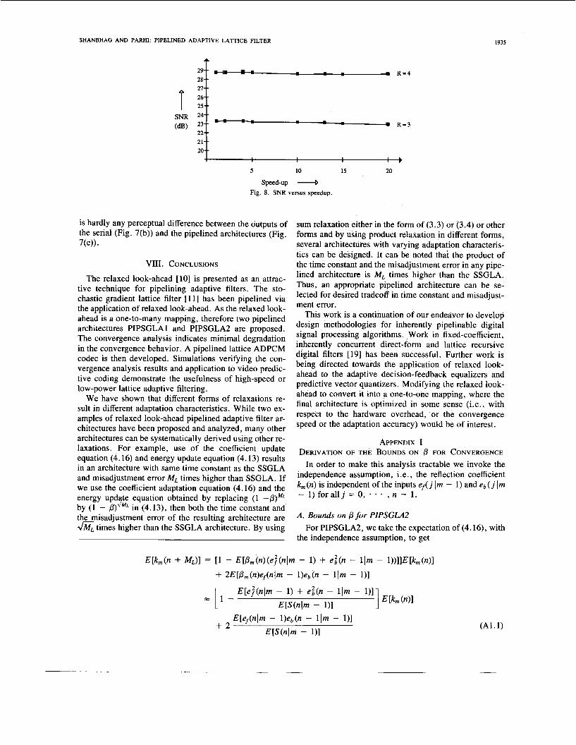
The original image has a frame-size of 256 X 256, with 8 b per pixel (bpp) (see Fig. 7(a)). The pipelined ADPCM codec was employed to code and then reconstruct this image for different values of the speed-up. As discussed in Section V, the PIPSGLA2 has a degraded convergence speed as compared to SSGLA. This implies that as the speedup increases the signal-to-noise ratio at the codec output would decrease. Two sets of simulations with R = 3 and R = 4 were done for different speedups. The values for Ms and ML were obtained from Table 111. In Fig. 8, we show the trend in SNR as the speedup increases. It can

1 Fig. 7. Images: (a) original, (b) serial codec output, and (c) pipelined codec output.

be seen that for a speedup as high as 20, the loss in SNR (for R = 3) is 0.1 dB. For R = 4, this loss is 0.27 dB. Thus, we conclude that the SNR loss due to the application of relaxed look-ahead is minimal and leads to no per- .

zeptual degradation of image quality. In Fig. 7(b), we show the reconstructed image (R = 3)

for the serial ADPCM codec, which is equivalent to the pipelined ADPCM codec with a speedup of unity. From Fig. 8, the SNR for the serial ADPCM codec is 23.4 dB. The reconstructed image for a speedup of 20 is shown in Fig. 7(c), which has an SNR of 23.3 dB. Note that there

1935 SHANBHAG AND PARHI: PIPELINED ADAPTIVE LATTICE FILTER

29-- 28-- U-- 26-- 25- 24- 23- 22- 21-- 20--

4 S N R (dB1

A

- - - R = 4 . I

- - - - R = 3

1

is hardly any perceptual difference between the outputs of the serial (Fig. 7(b)) and the pipelined architectures (Fig. 7(c)).

VIII. CONCLUSIONS

The relaxed look-ahead [ lo] is presented as an attractive technique for pipelining adaptive filters. The stochastic gradient lattice filter [ 1 11 has been pipelined via the application of relaxed look-ahead. As the relaxed look- ahead is a one-to-many mapping, therefore two pipelined architectures PIPSGLA1 and PIPSGLA2 are proposed. The convergence analysis indicates minimal degradation in the convergence behavior. A pipelined lattice ADPCM codec is then developed. Simulations verifying the convergence analysis results and application to video predictive coding demonstrate the usefulness of high-speed or low-power lattice adaptive filtering.

We have shown that different forms of relaxations result in different adaptation characteristics. While two ex- amples of relaxed look-ahead pipelined adaptive filter architectures have been proposed and analyzed, many other architectures can be systematically derived using other relaxations. For example, use of the coefficient update equation (4.16) and energy update equation (4.13) results in an architecture with same time constant as the SSGLA and misadjustment error ML times higher than SSGLA. If we use the coefficient adaptation equation (4.16) and the energy update equation obtained by replacing (1 - / 3 )ML by (1 - /3)dML in (4.13), then both the time constant and the misadjustment error of the resulting architecture are a times higher than the SSGLA architecture. By using

sum relaxation eithet. in the form of (3.3) or (3.4) or other forms and by using product relaxation in different forms, several architectures with varying adaptation characteristics can be designed. It can be noted that the product of the time constant and the misadjustment error in any pipelined architecture is ML times higher than the SSGLA. Thus, an appropriate pipelined architecture can be se- lected for desired tradeoff in time constant and misadjustment error.

This work is a continuation of our endeavor to develop design methodologies for inherently pipelinable digital signal processing algorithms. Work in fixed-coefficient , inherently concurrent direct-form and lattice recursive digital filters [19] has been successful. Further work is being directed towards the application of relaxed look- ahead to the adaptive decision-feedback equalizers and predictive vector quantizers. Modifying the relaxed look- ahead to convert it into a one-to-one mapping, where the final architecture is optimized in some sense (i.e., with respect to the hardware overhead, or the convergence speed or the adaptation accuracy) would be of interest.

APPENDIX I DERIVATION OF THE BOUNDS ON /3 FOR CONVERGENCE

In order to make this analysis tractable we invoke the independence assumption, i.e., the reflection coefficient k, (n) is independent of the inputs ef( j Im - 1) and eb( j lm - 1) f o r a l l j = 0, * , n - 1.

A. Bounds on /3 for PIPSGLA2

the independence assumption, to get For PIPSGLA2, we take the expectation of (4.16), with

(Al . 1)


where E [ .] represents the expectation operator. Starting with the order-update equations (4.19), we,can

compute the gradient of E[ej(nIm - 1) + eg(nlm - 1)l with respect to k, (n). The optimum value of k, (n) (denoted as l ~ ~ , ~ ~ ~ ) obtained by equating this gradient to zero is given by

2E[ef(nlm - I)eb(n - llm - l)] ',,Opt = E[ej(nlm - 1) + eg(n - llm - l)]

. (A1.2)

Taking the expectation as n -+ 00 of (4.17), we get E[ej(nlm - 1) + eg(n - ~ ( m - I)]

. (A1.3) E[S(nlm - 111

Using (A1.2) and (A1.3), it is easy to write (Al . l ) as follows:

E[km (n + M L ) ~ - km,opt

P =

= 11 - Pl(E[kn(n)l - km,opJ- (A1.4) Hence, for convergence, it is sufficient that

-1 I 1 - 0 I 1 (A1.5) which is equivalent to

O I P I 2 . (A1.6) Note that (Al.6) also gives the bounds on for SSGLA. This is because substitution of M L = 1 in (A1.4) results in the equation for the convergence of the reflection coefficients of the SSGLA.

B. Bounds on P for PIPSGLAl

get Taking the expected value of both sides of (4.12), we

APPENDIX I1 DERIVATION OF THE CONVERGENCE TIME CONSTANTS We first derive the convergence time-constants Tk for

the convergence of the reflection coefficients.

A. Tk for SSGLA Rewriting (A1.4) with ML = 1, we get

E[km(n + 1)I - km,opt = [1 - Pl(E[km(n)l - km,opt)-

(A2.1)

Denoting E [k , (n)] - k,, opt by v (n), we get the following difference equation:

v(n + 1) = (1 - P)v(n). (A2.2)

Iterating (A2.2) n times, we get v(n + 1) = (1 - p)""v(o). (A2.3)

Equating the RHS (right-hand side) of (A2.2) to a decaying exponential with time-constant T k , we get

-1 Tk =

In (1 - PI 1 - _ - P '

(A2.4)

Thus, the reflection coefficient learning curve is inversely proportional to 0.

B. Tk for PIPSGLA2

Replacing E[k,(n)] - km,opt by v(n) in (Al.4), we get

(A2.5) v(n + ML) = (1 - P)v(n).

where E [.I represents the expectation operator.

fore, we may write (A1.7) as As km,opt for PIPSGLAl is also given by (Al.2), there-

E[km(n + M L ) ~ - km,opt

= [1 - M L ( ~ - (1 - P > M L ) ~ ( ~ [ k m ( n ) ~ - km,opt>. (Al.8)

For the LHS of (Al.8) to converge to zero it is sufficient that

-1 I 1 - ML(1 - (1 - P)ML) I 1 (A1.9) simplifying the inequality (Al.9) results in the following bounds on 0:

O I P I - . (Al. 10) 2 MZ

(Al.7)

The characteristic equation F ( y ) of (A2.5) is

(A2.6) yML - (1 - 0) = 0.

Hence, the solution to (A2.5) is given by ML- I

v(n) = c (v):cl (A2.7)

where Cl's are constants to determined by the specified initial conditions, and ( v ) , ( i = 0, 1, - , ML - 1) are the roots of (A2.6), given by

I = o

( v ) i = (1 - P)"ML exp (21. (A2.8)

By fitting (A2.7) with a decaying exponential with time-

-


constant Tk, we get APPENDIX 111 DERIVATION OF THE MISADJUSTMENT EXPRESSIONS In order to get closed form expressions for the misad-

justment of SSGLA, PIPSGLA1, and PIPSGLA2, we need to make certain simplifying assumptions. In particular, the independence assumptions outlined in Section V , are often invoked. In addition, let

- ML In (1 - PI ML P '

Tk =

(A2.9) - - I

C. Tk for PIPSGLAI Repeating the analysis done for PIPSGLA2 in the pre-

vious subsection on (Al.8) we get a: = E[e j (n (m - l)] = E[ei (n lm - l)] (A3.1)

v ( n + M ~ ) = (1 - ~ ~ ( 1 - (1 - P ) M L ) ) ~ ( , ) . (A2.10)

The solution to the characteristic equation of (A2.10) is given by

ML - I

represent the input signal power. Before the misadjustment expressions are derived, we develop some preliminary expressions for fourth-order statistics in terms of second-order ones. All the expectations in this Appendix are in the limit as n + 00.

A. Preliminaries

the following is true:

v ( n ) = c (v):c, (A2.11)

where again C,'s are to determined by the initial conditions, and ( v ) , ( i = 0, 1, * * * , ML - 1) are the roots of the characteristic equation of (A2. lo), and are given by

( V I , = (1 - ML(l - (1 - p ) ~ l > ) ' / ~ ' exp lM,j.

r = O

If XI, X2, X3, and X4 are jointly Gaussian variables then

E[XI x2x3x41 = E[XI &IE[X3X4I E [ X I X ~ I E [ X ~ X ~ ] 2 xi

+ E [XI &]E 1x2 X3I + (A3.2)

Employing (A3.2) and the expression for k,,OPt ((Al.2)), it is trivial to show the validity of the following:

E[ef (n(m - l)eb(n - Ilm - 111 = k,,optu: (A3.3a)

(A2.12)

Fitting a decaying exponential envelope we get the required time constant as

- M,

= [I - k i ,opt + var (k , (n) ) + v2(n)] Thus, the misadjustment 312 for a lattice stage is given by E [ e j ( n ( m - 111. (A2.14)

Assume that the variance of k, (n) (var(km (n))) has a constant value equal to var (k , (00)) and that the input to the lattice stage is stationary. Therefore, we see from (A2.14) Hence, all that remains to be done is to calculate the that the convergence speed of E[ej(nlm)] is governed by steady-state variance of the reflection coefficient var the rate at which v2(n ) approaches zero. Thus, the mean- (k , (00)) . To simplify notation in the following analysis, squared error-time-constant T , , ~ would be half of that of we represent ef(nlm - 1) by e f , eb(nlm - 1) by e b and T k . S(nlm - 1) by S .

1938 IEEE TRANSACTIONS ON SIGNAL PROCESSING, VOL. 41, NO. 5, MAY 1993

B. Misadjustment Expression for SSGLA

it can be shown that

of (A3.1 l ) , we get

Taking the expectation of (4.2) in the limit as n + 03, var (km(m)) = (1 - 2p + P2> var ( h ( O 3 ) ) + P2ki,opt

(8 + 4ki,0pt)

4p2(1 + 2ki,opt) 24P2ki,0pt - + (8 + 4ki,0pt)'

= p. (A3.6) E [ @ ; + e31

E ( S ) (A3.12)

Finally, we need to derive the expression for E[S2(n lm - l)] by squaring (4.2) first and then taking its expectation. This gives

E[S21 = (1 - P)2E[S21 + 2(1 - P)E[S(efl + e t ) ]

+ E[(ef + (A3.7)

Multiplying (4.2) by S(nlm - 1) and taking its expectation, we get

E[S(e ; + e ; ) ] = P E [ S 2 ] . (A3.8)

If we now substitute (A3.8) and (A3.3(d)) into (A3.7). we get the desired expression

It is now possible to simplify (A3.12) to get the analytical expression for var (k , (03)) shown below:

P(1 - k;,opt)2

(2 - P)(2 + G , o p t ) * var (k,(oo)) = (A3.13)

From (A3.5) and (A3.13), the misadjustment of SSGLA is given by

As all the expectations are taken in the limit as n + 03,

therefore, the analysis for SSGLA is also applicable to PIPSGLA2. Hence, the misadjustment expression for PIPSGLA2 is the same as that for SSGLA.

C. Misadjustment Expression for PIPSGLAl The deviation of 3npIpI proceeds in a manner analogous

to that of 3ns. The expectation of (4.13) in the limit as n + 03 gives

(8 + 4ki,0pt)

P2 U:. (A3.9)

We are now in a position to compute the steady-state

E [ S 2 ] =

= 1 - (1 - p p variance of the reflection coefficient. Subtracting k,, opt

from both sides of (4.1) and squaring, we get E [ @ ; + e31

E ( S ) (km(n + 1) - km.opt)* = y . (A3.15)

The expression for E [ S 2 ( n ( m - l)] is given by 4e;e i

S2 U:. (A3.16)

= ( 1 - 3 + 5 r k i ( n ) + - + k i , o p t (8 + 4kkOpt) E[S2I = - 2

Y The rest of the derivation is identical to that shown in the preceding subsection, and is not repeated. Subtracting k,,OPt fr6m both sides of (4.13), squaring and then taking the expectation, we get

2 2 M L Y ( ~ - kqopt) var &(a)) = . (A3.17)

(A3.10) (2 - MLY)(2 + k;,opt)

+ 2mi.opt. (A3.11)

Adding and subtracting (1 - 2p + /32)ki,opt on the RHS

Therefore, the adjustment of PIPSGLAl is given by

Thus, (A3.14) and (A3.18) are the desired expressions for the misadjustments of SSGLA and PIPSGLAl, respectively. The misadjustment for PIPSGLA2, as mentioned before, is the same as that of SSGLA.

ACKNOWLEDGMENT The authors acknowledge the constructive criticisms of

an anonymous reviewer which were instrumental in im- proving the contents of this paper.

SHANBHAG AND PARHI: PIPELINED ADAPTIVE LATTICE FILTER I939

REFERENCES [ I ] K. K . Parhi, “Algorithm transformation techniques for concurrent

processors,” Proc. IEEE, vol. 77, pp. 1879-1895, Dec. 1989. 121 K. K. Parhi and D. G. Messerschmitt. “Pipeline interleaving and

parallelism in recursive digital filters-Part I: Pipelining using scat- tered look-ahead and decomposition,” IEEE Trans. Acoust., Speech, Signal Processing, vol. 37, pp. 1099-1 117, July 1989.

[3] K. K. Parhi and D. G. Messerschmitt, “Pipeline interleaving and parallelism in recursive digital filters-Part 11: Pipelined incremental block filtering,” IEEE Trans. Acoust., Speech, Signal Processing,

[4] K. K. Parhi, “Pipelining in dynamic programming architectures,” IEEE Trans. Signal Processing, vol. 39, pp. 1442-1450, June 1991.

[SI K. K. Parhi, “Pipelining in algorithms with quantizer loops,” IEEE Trans. Circuits Syst., vol. 38, pp. 745-754, July 1991.

[6] K. K. Parhi, “High-speed VLSI architectures for Huffman and Vi- terbi decoders,” IEEE Trans. Circuits Syst. II: Analog and Digital Signal Processing, vol. 39, pp. 385-391, June 1992.

[7] H.-D. Lin and D. G. Messerschmitt, “Finite state machine has un- limited concurrency,” IEEE Trans. Circuits Syst . , vol. 38, pp. 465- 475, May 1991.

[8] K. K. Parhi and D. G . Messerschmitt, “Concurrent cellular VLSI adaptive filter architectures,” IEEE Trans. Circuits Sysr., vol. 34,

[9] T. Meng and D. G. Messerschmitt, “Arbitrarily high sampling rate adaptive filters,” IEEE Trans. Acoust., Speech, Signal Processing, vol. 35, pp. 455-470, Apr. 1987.

[IO] N. R. Shanbhag and K. K. Parhi, “A pipelined LMS adaptive filter architecture,” in Proc. 25th Asilomar Con$ Signals, Syst . , Comput.. Pacific Grove, CA, Nov. 1991, pp. 668-672.

[ 1 I] M. L. Honig and D. G. Messerschmitt, Adaptive Filters: Structures. Algorithms, and Applications.

[I21 N. R. Shanbhag and K. K. Parhi, “A pipelined adaptive lattice filter architecture: Theory and applications,” in Proc. EUSIPCO ’92, Brussels, Belgium, Aug. 1992.

[13] N. R. Shanbhag and K. K. Parhi, “A high-speed architecture for ADPCM coder and decoder,” in Proc. I992 IEEE Int. Symp. Circuits Syst., San Diego, CA, pp. 1499-1502.

[14] G. A. Clark, S. K. Mitra, and S. R. Parker, “Block implementation of adaptive digital filters,” IEEE Trans. Acoust., Speech, Signal Pro- cessing, vol. 29, pp. 744-752, June 1981.

[15] S. Theodoridis, “Pipeline architecture for block adaptive LS FIR filtering and prediction,” IEEE Trans. Acoust., Speech, Signal Pro- cessing, vol. 38, pp. 81-90, Jan. 1990.

[16] J. M. Cioffi, P. Fortier, S. Kasturia, and G. Dudevoir, “Pipelining the decision feedback equalizer,” presented at the IEEE DSP Work- shop, 1988.

[17] A. Gatherer and T. H.-Y. Meng, “High sampling rate adaptive decision feedback equalizer,” in Proc. IEEE ICASSP ’90, pp. 909-912.

[18] A. P. Chandrakasan, S. Sheng, and R. W. Brodersen, “Low power CMOS digital design,” IEEE J . Solid-State Circuits, vol. 27, pp. 473-484, Apr. 1992.

1191 J . 4 . Chung and K. K. Parhi, “Design of pipelined lattice IIR digital filters,” in Proc. 25th Asilomar Con$ Signals, Syst., Comput., Pa- cific Grove, CA, Nov. 1991, pp. 1021-1025.

vol. 37, pp. 1118-1 134, July 1989.

pp. 1141-1151, Oct. 1987.

Boston: Kluwer, 1984.

Naresh R. Shanbhag (S’86) was born on July 2, 1966 in India. He received the B. Tech. degree in electrical engineering from the Indian Institute of Technology, New Delhi, India, in 1988, and the M.S. degree in electrical engineering from Wright State University, Dayton, OH, in 1990. Cur- rently, he is working towards the Ph.D. degree in electrical engineering at the University of Min- nesota, Minneapolis. His research interests are in the general area of VLSI architectures and algorithms for signal processing which includes the

design of high-speed algorithms for speech and image compression, adaptive filtering, and channel equalization. In addition, he is also interested in efficient VLSI implementation methodologies for digital signal processing algorithms.

Keshab K. Parhi (S’85-M’88-SM’91) received the B. Tech. (Honors) degree from the Indian In- stitute of Technology, Kharagpur, India, in 1982, the M.S.E.E. degree from the University of Penn- sylvania, Philadelphia, in 1984, and the Ph.D. degree from the University of California, Berke- ley, in 1988.

He is currently an Associate Professor of Elec- trical Engineering at the University of Minnesota, Minneapolis. He has held short-term positions at the NEC C&C Research Laboratories. Kawasaki.

Japan, AT&T Bell Laboratories, Holmdel, NJ, and the IBM T. J. Watson Research Center, Yorktown Heights, NY, and has been a consultant to U.S. West Advanced Technologies. His research interests include concurrent algorithm and architecture designs for communications, signal and image processing systems, digital integrated circuits, VLSI digital filters, computer arithmetic, high-level DSP synthesis, and multiprocessor proto- typing and task scheduling for programmable software systems. He has published over 90 papers in these areas.

Dr. Parhi received the 1992 Young Investigator Award of the National Science Foundation, the 1992-1994 McKnight-Land Grant Professorship of the University of Minnesota, the 1991 Paper Award from the IEEE Sig- nal Processing Society (for his papers on pipeline interleaving and parallelism in recursive digital filters published in the July 1989 issue of the IEEE TRANSACTIONS ON SIGNAL PROCESSING), the 1991 Browder Thompson Prize Paper Award of the IEEE (for his paper on algorithm transformations published in the December 1989 issue of the PROCEEDINGS OF THE IEEE), the 1989 Research Initiation Award of the National Science Foundation, and the 1987 Eliahu Jury Award for Excellence in Systems Research and the 1987 Demetri Angelakos Award for altruistic activities afforded fellow graduate students of the University of California (UC), Berkeley, where he was a UC Regents Fellow and an IBM Graduate Fellow. He is a former Associate Editor for Image Processing and VLSI Applications for the IEEE TRANSACTIONSON CIRCUITS A N D SYSTEMS, and is currently an Editor for the Journal of VLSI Signal Processing. He is a member of Eta Kappu Nu and the Association for Computing Machinery.

a pipelined adaptive lattice filter architecture - parhi

Documents

pipelining of adaptive

parallel processing

application of relaxed

approximate form of

hardware complexity

hardware requirements

level of pipelining

high hardware com plexity