a practical algorithm for rendering all-frequency...

A Practical Algorithm for Rendering All-FrequencyInterreflectionsKUN XU and YAN-PEI CAO and LI-QIAN MATNList, Department of Computer Science & Technology, Tsinghua University, BeijingZHAO DONGCornell UniversityRUI WANGUniversity of MassachusettsandSHI-MIN HUTNList, Department of Computer Science & Technology, Tsinghua University, Beijing

Algorithms for rendering interreflection (or indirect illumination) effectsoften make assumptions about the frequency range of the materials’ re-flectance properties. For example, methods based on Virtual Point Lights(VPLs) and global photon maps perform well for diffuse and semi-glossymaterials but not so for highly-glossy or specular materials; the situationis reversed for methods based on ray tracing and caustics photon maps. Inthis paper, we present a practical algorithm for rendering interreflection ef-fects at all frequency scales. Our method builds upon a Spherical Gaussianrepresentation of the BRDF. Our main contribution is a novel mathemati-cal development of the interreflection equation. This allows us to efficientlycompute the one-bounce interreflection from a triangle to a shading pointthrough an analytic formula combined with a piecewise linear approxima-tion. We show through evaluation that this method is accurate for a widerange of BRDF parameters. Our second contribution is a hierarchical inte-gration method to handle a large number of triangles with bounded error.Finally, we have implemented the algorithm on the GPU, achieving near-interactive rendering speed for a variety of scenes.

Categories and Subject Descriptors: I.3.7 [Computer Graphics]: Three-Dimensional Graphics and Realism—Color, shading, shadowing, and tex-ture

General Terms: Rendering

Additional Key Words and Phrases: Interreflections, Global Illumination,Spherical Gaussian, GPU

ACM Reference Format:

Permission to make digital or hard copies of part or all of this work forpersonal or classroom use is granted without fee provided that copies arenot made or distributed for profit or commercial advantage and that copiesshow this notice on the first page or initial screen of a display along withthe full citation. Copyrights for components of this work owned by othersthan ACM must be honored. Abstracting with credit is permitted. To copyotherwise, to republish, to post on servers, to redistribute to lists, or to useany component of this work in other works requires prior specific permis-sion and/or a fee. Permissions may be requested from Publications Dept.,ACM, Inc., 2 Penn Plaza, Suite 701, New York, NY 10121-0701 USA, fax+1 (212) 869-0481, or [email protected]© YYYY ACM 0730-0301/YYYY/12-ARTXXX $10.00

DOI 10.1145/XXXXXXX.YYYYYYYhttp://doi.acm.org/10.1145/XXXXXXX.YYYYYYY

1. INTRODUCTION

Accurate rendering of interreflection (or indirect illumination) ef-fects has been a long-standing challenge in computer graphics re-search, particularly when the materials can vary across a varietyof different types, from diffuse to semi-glossy and to highly glossy.This wide range of frequency scales poses a great challenge for ren-dering algorithms. Many existing algorithms are efficient for only aspecific range of materials. For example, methods based on VirtualPoint Lights [Keller 1997] and global photon maps [Jensen 2001]perform well for diffuse and semi-glossy materials, but becomeincreasingly inefficient for highly-glossy or nearly specular mate-rials. This is mainly because these methods represent the sourceof indirect illumination using a discrete point set. This works wellwith diffuse materials, due to their low-frequency and smooth fil-tering nature. However, for highly-glossy materials, these methodsrequire a significantly larger number of discrete points, reducingthe computation performance and increasing the storage size.

On the other hand, methods based on path tracing [Kajiya 1986]and caustics photon maps [Jensen 2001] are efficient for highly-glossy and specular materials, but the efficiency drops significantlywhen the materials become diffuse or semi-glossy. This is mainlybecause these methods stochastically trace light rays upon reflec-tions or refractions from the materials. Therefore highly-glossy ma-terials lead to lower variance in the computation, reducing the ren-dering noise; conversely, nearly diffuse materials lead to high vari-ance and consequently increased rendering noise.

These limitations are fundamentally due to the lack of an algo-rithm that can efficiently handle a wide range of different materials,including both the diffuse and the specular ends. This is a commonissue in rendering research. Consequently, a scene that consists ofmixed materials (i.e. at different frequency scales) often requiresspecial care and the combination of several algorithms, each ofwhich deals with a separate frequency range. This results in in-creased algorithm complexity, and makes it difficult to ensure allindividual algorithms produce consistent results.

In this paper, we present a practical algorithm for rendering in-terreflection effects at all frequency scales. Our method builds upona Spherical Gaussian (SG) representation of the BRDF [Wang et al.2009]. By changing the support size of the Spherical Gaussian, thisrepresentation can faithfully reproduce BRDFs at a wide range offrequency (i.e. glossiness) levels. Our main contribution is a novelmathematical development of the interreflection equation. Specifi-

ACM Transactions on Graphics, Vol. VV, No. N, Article XXX, Publication date: Month YYYY.

2 • Xu et al.

(a) ring

(b) dragon (c) airplane (d) magic cube (e) bunny (f) table

Fig. 1: Our algorithm achieves near-interactive rendering speed of one-bounce interreflections with all-frequency BRDFs. The top row showscaustics on the plane where the BRDF of the ring varies from highly specular to diffuse. The bottom row shows various interreflection effects,such as indirect highlight (b), diffuse reflection (c), glossy reflection (d), and under different types of lights, such as local lights (e) andenvironment lights (f). Our algorithm runs at 0.4∼4 fps for all the above scenes.

cally, by representing the BRDF and lighting both using SGs, wederive an analytic formula for the one-bounce interreflection from atriangle to a shading point, and accurately estimate the result usinga piecewise linear approximation. We show through evaluation thatthis method performs well for a wide range of BRDF parameters,thanks to the analytic derivation.

In practical applications, however, we need to consider scenesthat consist of more than a few triangles. To improve the efficiencyof our algorithm, we present a hierarchical integration method tohandle a large number of triangles. The hierarchical integration iscomputed with bounded error. Finally, we have implemented thealgorithm on the GPU, achieving near-interactive rendering speedfor a variety of scenes. Figure 1 shows several examples.

2. RELATED WORKS

Rendering interreflection (or indirect illumination) effects is a clas-sic problem in computer graphics. A complete review is beyond thescope of this paper. We refer readers to [Ritschel et al. 2012] for acomprehensive survey. This section covers the most relevant workto ours. For clarity, we refer to light bouncing surfaces as reflectorsand final shading surfaces as receivers.

Virtual Point Lights (VPLs). An efficient solution for comput-ing interreflections is by representing the indirect lighting as a setof virtual point lights (VPLs). Instant radiosity [Keller 1997] isa classic VPL-based technique. It creates VPLs by tracing pathsfrom the primary lights, and uses shadow map algorithms to esti-mate the total illumination contribution from all VPLs to a shadingpoint. The step of estimating the contributions from all VPLs iscommonly known as final gathering. To achieve high-quality re-sult, a large number of VPLs are usually necessary. Therefore achallenge is how to accelerate the final gathering. Lightcuts [Wal-ter et al. 2005; Walter et al. 2006] constructs a hierarchical struc-

ture of VPLs to compute final gathering at sublinear cost. Row-column sampling [Hasan et al. 2007] and LightSlice [Ou and Pel-lacini 2011] reduce the computation cost by exploiting the low-rank structure of the light transport matrix. Traditional VPL-basedmethods are limited to diffuse or semi-glossy reflectors. To addressthis limitation, Hasan et al. [2009] presented virtual spherical lightsto support glossy reflectors. Davidovic et al. [2010] separate lighttransport into low-rank (global) and high-rank (local) components,and employ a different method for each component to account fordetailed glossy interreflections. Recently, Walter et al. [2012] pro-pose bidirectional lightcuts to reduce the bias in VPL-based ren-dering by introducing virtual sensor points on eye paths. While ac-curate, these VPL-based methods perform in offline speed, takingminutes or hours to run. In addition, highly glossy receivers typi-cally pose a big challenge as they require a large number of VPLs.

Photon Mapping. Photon mapping [Jensen 2001] first traces par-ticles from the primary lights to construct photon maps; then in thesecond pass, it performs ray tracing and estimates indirect illumina-tion on non-specular receivers using photon density estimation. Byexploiting the GPU, photon mapping can achieve interactive per-formance [Purcell et al. 2003; Wang et al. 2009; Fabianowski andDingliana 2009; McGuire and Luebke 2009; Hachisuka and Jensen2010], including both caustics and indirect illumination. However,these methods usually require the reflectors to be either diffuseor specular. Semi-glossy reflectors lead to significantly increasedcomputation cost.

Precomputed Radiance Transfer (PRT). Precomputed RadianceTransfer (PRT) [Sloan et al. 2002] achieves real-time indirect light-ing of static scenes by precomputing light transport matrices andcompressing them using a suitable basis set to exploit the low-dimensional structure of the matrices. PRT has been extended toachieve interreflection effects with dynamic BRDFs [Sun et al.


A Practical Algorithm for Rendering All-Frequency Interreflections • 3

2007; Ben-Artzi et al. 2008; Cheslack-Postava et al. 2008] underthe static scene assumption. Interreflections in dynamic scenes havealso been studied [Iwasaki et al. 2007; Pan et al. 2007], but limitedto low-frequency effects.

Interactive GI. Work on interactive global illumination (GI) hasa rich history. Dachsbacher and Stamminger [2005] introducedreflective shadow maps (RSM) where pixels in the shadow mapare considered indirect light sources. This method gathers low-resolution indirect lighting from the RSM and obtains high res-olution result using screen-space interpolation. While interactive,it is limited to diffuse reflectors and ignores indirect shadows.Later, Dachsbacher and Stamminger [2006] presented a methodto include non-diffuse reflectors by splatting the radiance contribu-tion from each pixel. However, it only supports diffuse receivers.Ritschel et al. [2008] presented imperfect shadow maps to approxi-mate indirect visibility for VPLs and achieved interactive GI usinga small number of VPLs. It is limited to low-frequency reflectioneffects. Later, Ritschel et al. [2009] introduced the micro-renderingtechnique for high-quality interactive GI. Final gathering at eachshading point is efficiently computed using hierarchical point ras-terization into a micro-buffer. The micro-buffer can be warped toaccount for BRDF importance. As a result it supports receivers withglossy BRDFs. However, the reflector is restricted to diffuse or low-frequency BRDFs. Laurijssen et al. [2010] proposed a method forinteractively rendering indirect highlights, accounting for glossy toglossy paths. However, it is not suitable for diffuse receivers. Re-cently, Loos et al. [2011] presented Modular Radiance Transfer forreal-time indirect illumination, but this method is limited to low-frequency effects. Finally, there are many image-based methods forefficiently rendering caustics [Wyman and Davis 2006; Shah et al.2007], but these techniques are aimed for perfectly specular reflec-tors.

Reflections/Refractions. Using Fermat’s theorem, researchershave employed differential geometry [Mitchell and Hanrahan1992] and Taylor expansion [Chen and Arvo 2000] to find reflec-tion points on implicit curved reflectors. In addition, many meth-ods [Ofek and Rappoport 1998; Roger and Holzschuch 2006] havebeen presented for generating the specular reflections from trian-gle meshes. Walter et al. [2009] proposed an efficient method forfinding refracted connecting paths from triangle meshes. However,these methods assume perfect reflection/refraction, and it is unclearhow to extend them to handle glossy materials.

Spherical Gaussians (SGs). Spherical Gaussians (SGs) provideflexible support sizes and closed-formed solutions for comput-ing function products and integrals. Thus they have been widelyadopted for representing spherical functions, such as environmentlighting [Tsai and Shih 2006] and BRDFs [Wang et al. 2009]. Wanget al. [2009] approximate the normal distribution of a microfacetBRDF using sums of SGs. They demonstrated that such approxi-mation is accurate for representing a wide range of parametric andmeasured BRDFs. They make use of this property to achieve real-time all-frequency rendering of dynamic BRDFs under the staticscene assumption. However, this method only considers direct illu-mination, while our method focuses on interreflections.

3. BACKGROUND

In this section, we review the necessary background of sphericalGaussians (SGs) representations and BRDF approximations.

SG Definition. A Spherical Gaussian (SG) is a function of unitvector v and is defined as:

G(v;p,λ ,c) = c · eλ (v·p−1) (1)

where unit vector p, λ , and c represent the center direction, band-width, and the scalar coefficient of the SG. For simplicity, we de-note G(v) = G(v;p,λ ,c) and G(v;p,λ ) = G(v;p,λ ,1). SGs havemany known properties. For example, the integral of SG has ana-lytic solutions, and the product of two SGs is still an SG. These areexplained in details in the Appendix.

BRDF Approximation. A BRDF is commonly represented as thesum of a diffuse component and a specular component:

ρ (i,o) = kd + ks ρs (i,o) (2)

where i, o are the incoming and outgoing directions; kd , ks arethe diffuse and specular coefficients. We approximate the specularcomponent (also called specular lobe) ρs using a single SG:

ρs (i,o)≈ G(i;2(o ·n)n−o,λs)

where n is the surface normal, and λs is the bandwidth whichcontrols the specular lobe size. Note that the diffuse componentkd can be treated as a special SG with a zero bandwidth: kd =G(i;2(o ·n)n−o,0,kd). Therefore the BRDF defined in Eq. 2 canbe re-written as the sum of two SGs:

ρ (i,o)≈1

∑j=0

G(

i;o j,λ j,c j)

(3)

where λ 0 = 0, c0 = kd , λ 1 = λs, c1 = ks, o0 = o1 = 2(o ·n)n−o.Note that the above SG approximation is a simplified version of themodel introduced by Wang et al. [2009]. As shown in their work,the specular component of commonly used parametric BRDFs,such as the Blinn-Phong and the Cook-Torrance models, can beaccurately approximated by one single SG. Even for more sophisti-cated BRDFs, such as measured ones, a small number of SGs usu-ally suffice to achieve highly accurate approximations.

4. ONE-BOUNCE INTERREFLECTION MODEL

Triangle T (reflector)

SG Light

receiver

x

o

r

l

n-i

y

T

nx

Fig. 2: Light path of one-bounce interreflection.

We start by deriving the one-bounce interreflection model fora single triangle reflector, as shown in Figure 2. Assuming a dis-tant incident SG light l with emitted radiance G(i; il ,λl) (Gl (i) forshort), given a triangle T with normal nT (referred to as the re-flector) and a shading point x with normal nx (referred to as thereceiver point), we aim to compute the outgoing radiance from x to


4 • Xu et al.

the view direction o due to the reflection of the SG light l from tri-angle T towards x. Note that all directions are defined in the globalframe.

To simplify the derivation, for now we assume there is no oc-clusion between the light, the reflector and the receiver (The incor-poration of visibility will be explained later in Section 6). We alsoignore texture data on the reflector, assuming that the reflector hasa uniform BRDF. The incorporation of texture will be explained inSection 5. The one-bounce outgoing radiance from x towards o canthen be computed as an integration over a spherical triangle:

Lx(o) =∫

ΩT

L(r)ρx (−r,o)max(−r ·nx,0)dr (4)

where r is the direction from a point y on the reflector triangle T tox, and the integral is over the spherical triangle ΩT subtended by T;ρx and nx are the BRDF and normal direction at the receiver pointx; L(r) is the reflected radiance from y to x, defined as:

L(r) =∫

Ω

Gl (i)ρT (i,r)max(i ·nT ,0)di (5)

where ρT ,nT are the BRDF and normal of triangle T , respectively,and Gl (i) = G(i; il ,λl) is the incident SG light as described before.

4.1 Evaluating the Reflected Radiance L(r)In this subsection, we will explain how to evaluate the reflectedradiance L(r) defined in Eq. 5. First, we represent the BRDFρT of the triangle T as a sum of SGs (as shown in Eq. 3):ρT (i,r) ≈ ∑

1j=0 G

(i;r j

T ,λj

T ,c jT

). For denotation simplicity, in the

following derivation, we omit the summation ∑1j=0 (·) over index j

and rewrite the BRDF approximation as ρT (i,r)≈G(i;rT ,λT ,cT )(GT (i) for short). This yields:

L(r)≈∫

Ω

Gl (i)GT (i)max(i ·nT ,0)di

Secondly, since the product of Gl (i) and GT (i) is still a SG (seeAppendix B), and the cosine factor max(i ·nT ,0) is very smooth,we assume it is constant across the support of the product SG andthus can be pulled out of the integral [Wang et al. 2009; Xu et al.2011] (also see Appendix D):

L(r)≈max(iT (r) ·nT ,0)∫

Ω

Gl (i) ·GT (i)di (6)

where iT (r) = (λl il +λT rT )/‖λl il +λT rT ‖ is the center directionof the product SG. As shown in Appendix C, the integral of theproduct SG can be well approximated by a single SG:∫

Ω

Gl (i) ·GT (i)di≈ cR (r)exp(λR (rT · il −1))

where cR (r) = 2πcT /‖λl il +λT rT ‖, λR = λT λl/(λT +λl). Be-sides, the dot product rT · il satisfies:

rT · il = (2(r ·nT )nT − r) · il = r · (2(il ·nT )nT − il) = r · iRwhere iR = 2(il ·nT )nT − il . Hence the integral of the product SGcan be rewritten as:∫

Ω

Gl (i) ·GT (i)di≈ cR (r)exp(λR (r · iR−1))

= cR (r)G(r; iR,λR)

By substituting the above Equation to Eq. 6, the reflected radianceL(r) can be finally evaluated as:

L(r)≈ F(r)G(r; iR,λR) (7)

where F(r) = cR(r)max(iT (r) ·nT ,0) is a function much smootherthan the SG. Thus the reflected radiance L(r) is evaluated as a linearsum of the product of a smooth function and an SG.

4.2 Evaluating the Interreflection Radiance Lx(o)

Now we explain how to evaluate the one-bounce outgoing radianceLx(o) defined in Eq. 4. Similar to before, we represent the BRDFρx at the receiver point x as a sum of SGs (as shown in Eq. 3):ρx (−r,o)≈∑

1j=0 G

(r;−o j

x,λj

x ,c jx

). For denotation simplicity, we

again omit the summation ∑1j=0 (·) over index j below, and substi-

tute the reflected radiance L(r) (Eq. 7) into Eq. 4:

Lx(o)≈∫

ΩT

H(r)G(r; iR,λR)G(r;−ox,λx,cx)dr

where H(r) = F(r) ·max(−r ·nx,0) is again a smooth function.Since the product of two SGs is still an SG (see Appendix B), theabove Equation can be rewritten as:

Lx(o)≈∫

ΩT

H(r)G(r;rh,λh,ch)dr

where G(r;rh,λh,ch) is the product of the two SGs in the aboveEquation. (The formulas for rh,λh and ch can be found in AppendixB.) Since function H is intrinsically smooth, we can pull it out ofthe integral and rewrite the above equation as:

Lx(o)≈ H(r′h)∫

ΩT

G(r;rh,λh,ch)dr (8)

The representative direction r′h used for querying the constant valueof function H is set to be a linear interpolation of the SG’s centerdirection rh and the direction from the origin to the center of thespherical triangle ΩT . The interpolation weight is determined bythe area size of ΩT and SG support. We adopt such an interpolationmethod because the optimal choice of the representative directionvaries in different scenarios. For example, if the spherical triangleis much larger than the support of SG (e.g. SG just spans a smallarea inside the spherical triangle), the best choice of the represen-tative direction is the SG center; Conversely, if the support of SG ismuch larger than the spherical triangle, the best choice is the trian-gle direction. The formula of r′h is described in Appendix G.

The remaining question in Eq. 8 is how to evaluate the integral ofan SG over a spherical triangle subtended by the planar triangle T .However, this integral does not have a closed-form solution. Fortu-nately, as shown in the following subsection, it can be reduced to a1D integral, which can then be evaluated using a piecewise linearapproximation.

4.3 Integrating an SG over a Spherical Triangle

Given an SG G(v;p,λ ), we want to derive how to integrate it overa spherical triangle ΩT , in other words, compute

∫ΩT

G(v;p,λ )dv.As shown in Figure 3(a), the local frame is defined by setting theSG center direction p as the zenith direction. Denote the the originof the unit sphere as O and the zenith point as P, and the vertices ofthe spherical triangle ΩT as A, B and C, respectively. It is obviousthat the spherical triangle ΩT satisfies:

ΩT = Ω4ABC = Ω4PBC−Ω4PAB−Ω4PCA

The plus/minus sign may vary depending on relative positions ofthe zenith point P and spherical triangle Ω4ABC (e.g. when P is in-side Ω4ABC, Ω4ABC = Ω4PBC + Ω4PAB + Ω4PCA). Without loss



O

Triangle T p p

AC

B

P

ΩT

O

v

CV

MB

P

φb

φc

θ

φ

θ φm ( )

(a) (b)

Fig. 3: Integrating an SG over a spherical triangle ΩT .

of generality, let us consider how to evaluate the integral over spher-ical triangle4PBC:

∫Ω4PBC

G(v;p,λ )dv. Using the coordinate sys-tem defined in Figure 3, we can rewrite the integral using the spher-ical coordinates to simplify the derivation.

As shown in Figure 3(b), denote the azimuthal angles of point Band C as φb and φc, respectively, the intersection point of an arbi-trary direction v with the unit sphere as V , the polar and azimuthal

angle of v as (θ ,φ). Since both arcs_PB and

_PC are longitude arcs,

we can rewrite the integral in spherical coordinates by integratingthe azimuthal angle from φc to φb:∫

Ω4PBC

G(v)dv =∫

φb

φc

(∫θm(φ)

0G(v;p,λ )sinθ dθ

)dφ

=∫

φb

φc

(∫θm(φ)

0eλ (cosθ−1) sinθ dθ

)dφ

where θm(φ) is the maximal allowed polar angle when the az-imuthal angle is φ . As shown in Figure 3(b), it is the polar angle

of the intersection point M of arc_BC and the longitude arc

_PV . It

is easy to find out that the inner integral of polar angle θ has ananalytic solution, so that the above equation can be rewritten as:∫

Ω4PBC

G(v)dv =∫

φb

φc

(− 1

λeλ (cosθ−1)|θm(φ)

0

)dφ

=1λ

∫φb

φc

(1− eλ (cosθm(φ)−1)

)dφ

Through some further derivations using basic geometric proper-ties, we found that the cosine of the maximal allowed polar anglecosθm(φ) can be written as (proof can be found in Appendix H):

cosθm(φ) = sin(φ +φ0)/√

m2 + sin2(φ +φ0) (9)

where the two parameters φ0 and m can be calculated through thespherical coordinates of the two vertices B and C. Putting every-thing together, the integral of G(v) can be rewritten as:

∫Ω4PBC

G(v)dv =φb−φc

λ− 1

λ

∫φb

φc

eλ

(sin(φ+φ0)√

m2+sin2(φ+φ0)−1)

dφ

=φb−φc

λ− 1

λ

∫φ2

φ1

fm,λ (φ)dφ (10)

where φ1 = φc + φ0, φ2 = φb + φ0, and the 1D function fm,λ (φ) isdefined as:

fm,λ (φ) = exp

λ

sinφ√m2 + sin2

φ

−1

(11)

m=0.1, =100

m=0.005, =100

m=0.01, =1000

m=0.02, =1000

fm,

−→ φ

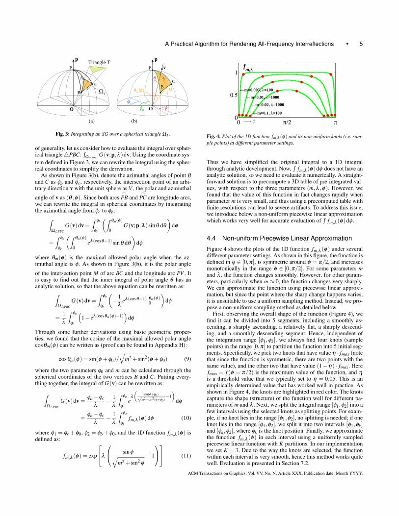
Fig. 4: Plot of the 1D function fm,λ (φ) and its non-uniform knots (i.e. sam-ple points) at different parameter settings.

Thus we have simplified the original integral to a 1D integralthrough analytic development. Now,

∫fm,λ (φ)dφ does not have an

analytic solution, so we need to evaluate it numerically. A straight-forward solution is to precompute a 3D table of pre-integrated val-ues, with respect to the three parameters (m,λ ,φ). However, wefound that the value of this function in fact changes rapidly whenparameter m is very small, and thus using a precomputed table withfinite resolutions can lead to severe artifacts. To address this issue,we introduce below a non-uniform piecewise linear approximationwhich works very well for accurate evaluation of

∫fm,λ (φ)dφ .

4.4 Non-uniform Piecewise Linear Approximation

Figure 4 shows the plots of the 1D function fm,λ (φ) under severaldifferent parameter settings. As shown in this figure, the function isdefined in φ ∈ [0,π], is symmetric around φ = π/2, and increasesmonotonically in the range φ ∈ [0,π/2]. For some parameters mand λ , the function changes smoothly. However, for other param-eters, particularly when m ≈ 0, the function changes very sharply.We can approximate the function using piecewise linear approxi-mation, but since the point where the sharp change happens varies,it is unsuitable to use a uniform sampling method. Instead, we pro-pose a non-uniform sampling method as detailed below.

First, observing the overall shape of the function (Figure 4), wefind it can be divided into 5 segments, including a smoothly as-cending, a sharply ascending, a relatively flat, a sharply descend-ing, and a smoothly descending segment. Hence, independent ofthe integration range [φ1,φ2], we always find four knots (samplepoints) in the range [0,π] to partition the function into 5 initial seg-ments. Specifically, we pick two knots that have value η · fmax (notethat since the function is symmetric, there are two points with thesame value), and the other two that have value (1−η) · fmax. Herefmax = f (φ = π/2) is the maximum value of the function, and η

is a threshold value that we typically set to η = 0.05. This is anempirically determined value that has worked well in practice. Asshown in Figure 4, the knots are highlighted in red color. The knotscapture the shape (structure) of the function well for different pa-rameters of m and λ . Next, we split the integral range [φ1,φ2] into afew intervals using the selected knots as splitting points. For exam-ple, if no knot lies in the range [φ1,φ2], no splitting is needed; if oneknot lies in the range [φ1,φ2], we split it into two intervals [φ1,φk]and [φk,φ2], where φk is the knot position. Finally, we approximatethe function fm,λ (φ) in each interval using a uniformly sampledpiecewise linear function with K partitions. In our implementationwe set K = 3. Due to the way the knots are selected, the functionwithin each interval is very smooth, hence this method works quitewell. Evaluation is presented in Section 7.2.


6 • Xu et al.

Summary. In this section, we derived the analytic formula for com-puting one-bounce interreflection from a triangle (Eq. 4) to a shad-ing point due to a distance SG light. Furthermore, we demonstratedthat this formula can be efficiently evaluated using a non-uniformpiecewise linear approximation of a 1D function (Eq. 11).

5. HIERARCHICAL STRUCTURE

In the previous section, we derived an analytical formula for com-puting the interreflection from a single reflector triangle to a shad-ing point. For simple scenes we can apply the formula to directlysum up the contribution from each triangle. However, the cost islinear to the number of triangles, thus this approach would performpoorly for complex scenes with many triangles.

Inspired by previous hierarchical integration methods, such ashierarchical radiosity [Hanrahan et al. 1991], the Lightcuts [Wal-ter et al. 2005] and the micro-rendering technique [Ritschel et al.2009], we also propose a hierarchical method to efficiently sumup the contribution from all triangles in the scene. Specifically, asshown in Figure 5(a), we organize the scene triangles into a binarytree. The leaf nodes are individual triangles, and the interior nodesare subsets of triangles, each owning the triangles that belong to itstwo child nodes. The binary tree is built in a top-down fashion dur-ing the scene initialization step. Starting from the root node, whichowns all the triangles, each node is recursively split into two childnodes until reaching the leaf node.

To define the splitting criterion, we first define a 6D feature(I,mn) for each triangle, where I is the triangle center (the scene’sbounding box is normalized to [−1,1]) and n is the triangle nor-mal. m is a scalar weights that controls the relative importance ofI and n, and we usually set it to m = 5. Next, the splitting is com-puted using the principal direction rule. Specifically, at every node,we compute the principal direction (using PCA) of the 6D featuresof all triangles belonging to that node, and perform a median splitalong the principal direction. This ensures that the splitting is donealong the direction of maximum variance. The result of the me-dian split produces two child nodes with equal number of triangles.For non-textured scene, each node stores the average center andnormal of its triangles, as well as a bounding box, a normal cone,and the total triangle area. See Figure 5(a) for illustration. To dealwith textured scene, each node additionally stores the average andthe largest/smallest texture color values of all the textures mappedon its triangles. The average texture color value is used to modulatethe radiance contribution of the node, while the largest/smallest tex-ture color values are used to estimate the error bound. These storedterms are used later to estimate the reflected radiance from the nodeto a receiver point, and the associated error bound.

During the rendering stage, we employ a similar strategy as in theLightcuts [Walter et al. 2005] to efficiently evaluate the one-bounceinterreflections. For each receiver point, we start from an initial cutthat contains only the root node of the binary tree, then iterativelyrefine it. At each iteration, we pick the node with the highest es-timated error and replace it by its two child nodes. The iterationstops either if the largest estimated error falls below a threshold (inour case, 1% of the total estimated reflected radiance), or a prede-fined maximum number of nodes in the generated cut is reached(1000 in our case). When the iteration terminates, we refer to theresulting cut as the reflector cut. The number of nodes in the cut isreferred to as cut size. Figure 5(b) shows an illustration. Note thatwhen reaching the leaf node during the iteration, we can directlyuse the interreflection model for a single triangle reflector to accu-rately evaluate its one-bounce contribution. However, this strategyonly works well for non-textured scenes since our derivations in

(b)

(d)

1

2 3

7654

1

2 3

6 754(a)

Bounding

Normal

(c)

Directioncone

-ox

Cone for Normal cone

il

Central cone

cone

box

rh

rh

iR

iR

iR

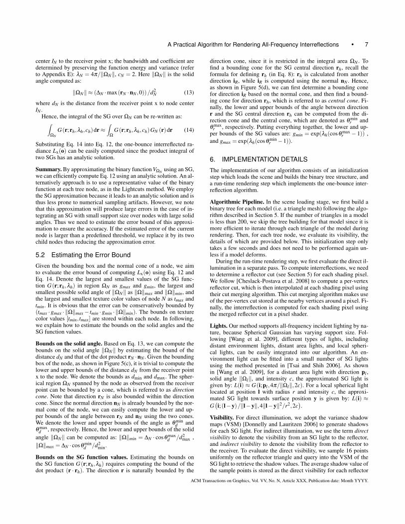
Fig. 5: Hierarchical structure and error bound estimation. (a) a binary treeof triangles showing the bounding box and normal cone stored at eachnode; (b) an example of reflector cut; (c) direction cone; (d) computingcentral cone from the normal cone.

Section 4 assumes that the reflector triangle has a uniform BRDFacross it without texture variations. Hence, when dealing with leafnode with a textured triangle, we still compute its error bound usingits stored texture info. If the estimated error bound is larger than apredefined threshold, we subdivide this triangle into 4 subtrianglesusing

√3−subdivision [Kobbelt 2000], and use the 4 subtriangles

to further evaluate one-bounce contributions. Such a dynamic sub-division strategy can be applied iteratively until the estimated errorbounds of the subdivided triangles are sufficiently small.

Next, we will explain in detail how to evaluate the estimated one-bounce radiance reflected by a node (in Section 5.1) and the asso-ciated error bound (in Section 5.2).

5.1 Estimating the Interreflected Radiance

Given a node N and a receiver point x, we estimate the radiancefrom x towards the view direction o, due to the reflection of an SGlight G(i;pl ,λl) from node N. To begin, we denote the center po-sition of node N as IN , its average triangle normal as nN , and itstriangle area as ∆N . Then, inspired by the micro-rendering tech-nique [Ritschel et al. 2009], the node N is treated as an “implicit”plane with center position IN , normal direction nN , area ∆N , andaverage texture color tN . Hence, we can reuse Eq. 8 derived for asingle triangle, only changing the integration area from a sphericaltriangle ΩT to a spherical region ΩN spanned by all the trianglesbelonging to node N:

Lx(o)≈ tN ·H(r′h)∫

ΩN

G(r;rh,λh,ch)dr (12)

However, since the shape of the spherical region ΩN is unknown(it is a spherical region subtended by a set of triangles), we can-not directly apply the piecewise linear approximation described inSection 4. To address this issue, we rewrite the integral of an SGover spherical region ΩN as the SG multiplied by a binary maskintegrated over the whole sphere :∫

ΩN

G(r;rh,λh,ch)dr =∫

Ω

G(r;rh,λh,ch)VΩN (r)dr

where Ω denotes the whole sphere, VΩN (r) is a binary functionthat indicates if a direction r is inside ΩN . We further approximateVΩN using an SG: VΩN (r) ≈ G(r;rN ,λN ,cN) (GN (r) for short).The center direction rN is set to be the unit direction from node



center IN to the receiver point x; the bandwidth and coefficient aredetermined by preserving the function energy and variance (referto Appendix E): λN = 4π/‖ΩN‖, cN = 2. Here ‖ΩN‖ is the solidangle computed as:

‖ΩN‖ ≈ (∆N ·max(rN ·nN ,0))/d2N (13)

where dN is the distance from the receiver point x to node centerIN .

Hence, the integral of the SG over ΩN can be re-written as:∫ΩN

G(r;rh,λh,ch)dr≈∫

Ω

G(r;rh,λh,ch)GN (r)dr (14)

Substituting Eq. 14 into Eq. 12, the one-bounce interreflected ra-diance Lx(o) can be easily computed since the product integral oftwo SGs has an analytic solution.

Summary. By approximating the binary function VΩN using an SG,we can efficiently compute Eq. 12 using an analytic solution. An al-ternatively approach is to use a representative value of the binaryfunction at each tree node, as in the Lightcuts method. We employthe SG approximation because it leads to an analytic solution and isthus less prone to numerical sampling artifacts. However, we notethat this approximation will produce large errors in the case of in-tegrating an SG with small support size over nodes with large solidangles. Thus we need to estimate the error bound of this approxi-mation to ensure the accuracy. If the estimated error of the currentnode is larger than a predefined threshold, we replace it by its twochild nodes thus reducing the approximation error.

5.2 Estimating the Error Bound

Given the bounding box and the normal cone of a node, we aimto evaluate the error bound of computing Lx(o) using Eq. 12 andEq. 14. Denote the largest and smallest values of the SG func-tion G(r;rh,λh) in region ΩN as gmax and gmin, the largest andsmallest possible solid angle of ‖ΩN‖ as ‖Ω‖max and ‖Ω‖min, andthe largest and smallest texture color values of node N as tmax andtmin. It is obvious that the error can be conservatively bounded by(tmax ·gmax · ‖Ω‖max− tmin ·gmin · ‖Ω‖min). The bounds on texturecolor values [tmin, tmax] are stored within each node. In following,we explain how to estimate the bounds on the solid angles and theSG function values.

Bounds on the solid angle. Based on Eq. 13, we can compute thebounds on the solid angle ‖ΩN‖ by estimating the bound of thedistance dN and that of the dot product rN ·nN . Given the boundingbox of the node, as shown in Figure 5(c), it is trivial to compute thelower and upper bounds of the distance dN from the receiver pointx to the node. We denote the bounds as dmin and dmax. The spher-ical region ΩN spanned by the node as observed from the receiverpoint can be bounded by a cone, which is referred to as directioncone. Note that direction rN is also bounded within the directioncone. Since the normal direction nN is already bounded by the nor-mal cone of the node, we can easily compute the lower and up-per bounds of the angle between rN and nN using the two cones.We denote the lower and upper bounds of the angle as θ min

d andθ max

d , respectively. Hence, the lower and upper bounds of the solidangle ‖ΩN‖ can be computed as: ‖Ω‖min = ∆N · cosθ max

d /d2max ,

‖Ω‖max = ∆N · cosθ mind /d2

min.

Bounds on the SG function values. Estimating the bounds onthe SG function G(r;rh,λh) requires computing the bound of thedot product (r · rh). The direction r is naturally bounded by the

direction cone, since it is restricted in the integral area ΩN . Tofind a bounding cone for the SG central direction rh, recall theformula for defining rh (in Eq. 8): rh is calculated from anotherdirection iR, while iR is computed using the normal nN . Hence,as shown in Figure 5(d), we can first determine a bounding conefor direction iR based on the normal cone, and then find a bound-ing cone for direction rh, which is referred to as central cone. Fi-nally, the lower and upper bounds of the angle between directionr and the SG central direction rh can be computed from the di-rection cone and the central cone, which are denoted as θ min

r andθ max

r , respectively. Putting everything together, the lower and up-per bounds of the SG values are: gmin = exp(λh(cosθ max

r − 1)) ,and gmax = exp(λh(cosθ min

r −1)).

6. IMPLEMENTATION DETAILS

The implementation of our algorithm consists of an initializationstep which loads the scene and builds the binary tree structure, anda run-time rendering step which implements the one-bounce inter-reflection algorithm.

Algorithmic Pipeline. In the scene loading stage, we first build abinary tree for each model (i.e. a triangle mesh) following the algo-rithm described in Section 5. If the number of triangles in a modelis less than 200, we skip the tree building for that model since it ismore efficient to iterate through each triangle of the model duringrendering. Then, for each tree node, we evaluate its visibility, thedetails of which are provided below. This initialization step onlytakes a few seconds and does not need to be performed again un-less if a model deforms.

During the run-time rendering step, we first evaluate the direct il-lumination in a separate pass. To compute interreflections, we needto determine a reflector cut (see Section 5) for each shading pixel.We follow [Cheslack-Postava et al. 2008] to compute a per-vertexreflector cut, which is then interpolated at each shading pixel usingtheir cut merging algorithm. This cut merging algorithm makes useof the per-vertex cut stored at the nearby vertices around a pixel. Fi-nally, the interreflection is computed for each shading pixel usingthe merged reflector cut in a pixel shader.

Lights. Our method supports all-frequency incident lighting by na-ture, because Spherical Gaussian has varying support size. Fol-lowing [Wang et al. 2009], different types of lights, includingdistant environment lights, distant area lights, and local spheri-cal lights, can be easily integrated into our algorithm. An en-vironment light can be fitted into a small number of SG lightsusing the method presented in [Tsai and Shih 2006]. As shownin [Wang et al. 2009], for a distant area light with direction pl ,solid angle ‖Ωl‖, and intensity c, the approximated SG light isgiven by: L(i) ≈ G(i;pl ,4π/‖Ωl‖,2c). For a local spherical lightlocated at position l with radius r and intensity c, the approxi-mated SG light towards surface position y is given by: L(i) ≈G(i;(l−y)/‖l−y‖,4‖l−y‖2/r2,2c

).

Visibility. For direct illumination, we adopt the variance shadowmaps (VSM) [Donnelly and Lauritzen 2006] to generate shadowsfor each SG light. For indirect illumination, we use the term directvisibility to denote the visibility from an SG light to the reflector,and indirect visibility to denote the visibility from the reflector tothe receiver. To evaluate the direct visibility, we sample 16 pointsuniformly on the reflector triangle and query into the VSM of theSG light to retrieve the shadow values. The average shadow value ofthe sample points is stored as the direct visibility for each reflector


8 • Xu et al.

triangle. To compute indirect visibility, we adopt a variant of imper-fect shadow maps (ISM) [Ritschel et al. 2008]. Specifically, duringscene loading step, we select 200 random sample points on eachmodel to represent the virtual light positions to capture the ISM atrun-time. For each node in the binary tree of the model, its closestthree sampled virtual lights are stored. Then, the center position ofthe node is projected onto the triangle plane spanned by the node’sthree samples, and the weight of each sampled light is computedas the barycentric coordinate of the projected position. During therun-time rendering stage, the ISM with a resolution 128× 128 isgenerated for each sampled virtual light. Next, during the evalua-tion of indirect illumination, after the reflector cut is determined,the visibility for each tree node is interpolated by the shadow val-ues from the ISMs, using the three closest sampled virtual lightsand the associated weights. The visibility approximation will beevaluated in Section 7.2.

Cut Selection. To improve performance, we implement the per-vertex cut selection algorithm using CUDA. The cut selection algo-rithm requires a priority queue structure to store tree nodes, sinceit needs to pick the node with the largest error and to replace itwith its two children. However, an accurate priority queue imple-mentation using CUDA is not yet efficient, thus we employ an ap-proximate priority queue. Specifically, we manage several (in ourimplementation, 5) ordinary queues with different priorities. Thequeue with the i-th priority stores nodes whose errors are largerthan 25−i%. For example, the first queue stores nodes with errorslarger than 16%, the second queue stores nodes with error largerthan 8%, and so on. At each step, we pick the front node in thequeue with the highest priority (e.g., pick from the first queue if itis non-empty, otherwise pick from the second queue, and so on) andsplit it into two child nodes. The two child nodes are then pushedinto the queues with the corresponding priorities according to theirerrors. Note that, for simple scenes without a tree structure, the per-vertex cut selection is not necessary.

Final Shading. The final one-bounce interreflection is evaluated ina pixel shader. At each pixel, the required data of its reflector cut,including positions, normals, BRDFs, and direct visibility of eachcut node, as well as the SG lights, are stored in textures and passedinto the pixel shader. Hence, the total contributions from all nodesin the cut to the pixel can be computed by iterating through everycut node. The non-linear piecewise linear approximation (in Sec-tion 4) for reflector triangles is used for leaf nodes, while the nodeapproximation (Eq. 14) is used for interior nodes. The contribu-tion of each node is modulated by the direct and indirect visibilitydescribed earlier. While direct visibility is obtained as a pass-in pa-rameter of each node, indirect visibility is obtained by interpolatingfrom the query shadow values using the ISMs.

7. RESULTS AND COMPARISONS

This section presents our results. Performance data is reported on aPC with Intel Xeon 2.27G CPU and 8 GB memory, and an NVIDIAGeforce GTX 690 graphics card. The algorithm is implemented us-ing OpenGL 4.0 and CUDA 4.1. The image resolution for all ren-dered results is 640× 480. We set the partition number K = 3 andthe error bound threshold to 1% for all examples. The performancedata is reported in Table I. For validation, we examine the accuracyof our mathematical model, as well as compare our results to theVPL-based method [Keller 1997], photon mapping [Jensen 2001],and the micro-rendering method [Ritschel et al. 2009].

scene #facesavg.

cut size fps shade.time

cut sel.time

magic cube 140 N/A 4.0 0.25s N/Atable 104 N/A 1.0 1.0s N/Aring 21k 151 0.7 1.0s 0.4s

dragon 26k 258 0.4 1.8s 0.5sairplane 20k 142 1.2 0.58s 0.19s

bunny & tweety 36k 316 0.3 2.5s 0.7skitchen 92k 489 0.12 6.9s 1.3ssponza 143k 566 0.09 9.0s 2.0s

Table I. : Performance of the results shown in this paper. From left to right,we give the name of the scene, the number of faces, average cut size, overallfps, final shading time and and cut selection time.

7.1 Results

Simple Scenes. We first verify our method using simple scenescontaining a couple hundred of triangles. Figure 6(a) shows resultsof a magic cube scene with varying BRDFs on the cube and onthe plane. In Figure 6(b), we show the results of a star scene anda kitchen scene under different environment lights represented by10 SGs. Note that in these examples, we demonstrate the capabilityof our algorithm in producing all-frequency interreflection effects,including diffuse to diffuse, diffuse to specular, and specular to dif-fuse (i.e. caustics) effects.Complex Scenes. Figure 1(a) shows the results of a ring with aBlinn-Phong BRDF changing from highly specular to purely dif-fuse. From left to right, the glossy shininess of the Blinn-PhongBRDF is set to n = 10000,1000,300,100 respectively, and the lastone is using a Lambertian BRDF. Note that our method producesconvincing caustics effects on the plane for all examples. Further,our method achieves smooth and coherent transitions (e.g. with-out flickering) while changing BRDF parameters (see the supple-mental video). Thus it is a single algorithm that can reproduce all-frequency reflection effects.

Figure 1(b,e) and Figure 6(b-d) demonstrate our method un-der different types of lights, including a local light (Figure 1(e)),SG lights with small support (Figure 1(c)) and large support (Fig-ure 6(c,d), as well as environment lights (Figure 6 (b)).Textured Scenes. Figure 7 shows results of complex texturedscenes. Note that our method performs well for such scenes withcomplex visibility and textures. Please refer to the accompanyingvideo for additional results.Performance. The performance data, including framerates, aver-age cut size (i.e. the average number of nodes in the reflector cut),time for final shading, and time for cut selection, is shown in Ta-ble I. We do not list the time for direct lighting and ISMs gener-ations since for all scenes it takes less than 0.1 seconds. Clearly,the bottleneck lies in the per-pixel final shading stage, especiallyfor complex scenes. Considering the sponza scene in Figure 7(b),the final shading stage takes 81% of the time on average, whileother steps, including the cut selection, ISMs generation and directlighting, take a total of 19% of the overall cost. This is because theaverage cut size increases with the number the faces. In the finalshading step, which is implemented in fragment shader, for eachpixel we need to loop all the nodes in its cut to compute the finalshading. However, such a shading computation adapts with the fastevolving GPU and can be greatly accelerated by next-gen many-core hardware.



(a) magic cube (b) environment lights

(c) dragon (d) bunny & tweety

Fig. 6: Additional rendering results. (a) A magic cube model with various BRDF settings (left: plane and cube are both diffuse; middle:cube is diffuse, plane is specular; right: plane is diffuse, cube is specular). (b) A star model and a table scene under environment light. Theenvironment lights are approximated using 10 SGs. (c) A dragon scene. (d) A “Bunny and Tweety” scene.

(a) kitchen (b) sponza

Fig. 7: Rendering results of complex textured scenes.

7.2 Comparisons

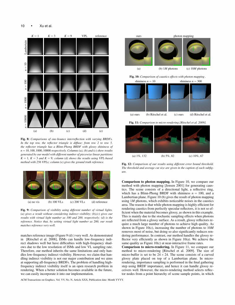
Accuracy of our model. In Figure 8, we show results of our one-bounce interreflection model using piecewise linear approximationwith different number of piecewise intervals (in Section 4.4). Wefurther compare our results with results generated by a VPL-basedmethod [Keller 1997] and the path traced reference. The test sceneconsists of a single equilateral triangle placed perpendicular to thereceiver plane, and a directional light at a 45 degree angle to theground plane. The ground (receiver) plane has a Lambertain BRDFand we only show the interreflection (i.e. no direct illumination)from the triangle to the plane in this figure.

In Figure 8, from the top row to the bottom row, the BRDF of thereflector triangle varies from purely diffuse to highly specular. Notethat our result with partition number K = 3 (column (b)) already

matches the reference image (column (e)) very well under all testedBRDFs. In contrast, the VPL-based method (column (d)) with 256VPLs works well for only low-frequency BRDFs, while producingsevere artifacts when the shininess parameter n≥ 10. This is mainlydue to the limited number of VPLs, which must be significantlyincreased for highly-glossy BRDFs.Accuracy of visibility approximation. Recall that we randomlysample some (typically 200) virtual lights (VLs) on each modeland generates one 128×128 ISM for each VL. Visibility betweenthe receiver point and each node/triangle is computed by interpo-lating the queried shadow values from three nearest VLs. Hence,the number of VLs affects the accuracy of the indirect visibility.In Figure 9, we evaluate the indirect visibility approximation usedin our method. Notice that our result with 200 VLs (Figure 9 (c) )


10 • Xu et al.

K = 1 K = 3 K = 9 VPL reference

Lam

bert

ain

n=

10n

=10

0n

=10

00n

=10

000

(a) (b) (c) (d) (e)

Fig. 8: Comparisons of one-bounce interreflection with varying BRDFs.In the top row, the reflector triangle is diffuse; from row 2 to row 5,the reflector triangle has a Blinn-Phong BRDF with glossy shininess ofn = 10,100,1000,10000 respectively. Columns (a), (b) and (c) show resultsgenerated by our model with different number of piecewise linear partitionsK = 1, K = 3 and K = 9; column (d) shows the results using VPL-basedmethod with 256 VPLs; column (e) gives the ground truth reference.

(a) no vis (b) 100 VLs (c) 200 VLs (d) reference

Fig. 9: Comparison of visibility using different number of virtual lights.(a) gives a result without considering indirect visibility; (b),(c) gives ourresults with virtual light number as 100 and 200, respectively; (d) is thereference. Notice that, by setting virtual light number as 200, our resultmatches reference very well.

matches reference image (Figure 9 (d) ) very well. As demonstratedin [Ritschel et al. 2008], ISMs can handle low-frequency indi-rect shadows well but have difficulties with high-frequency shad-ows due to the low resolution of ISMs and low VL sampling rate.Therefore, our method inherits the same limitations and only han-dles low-frequency indirect visibility. However, we claim that han-dling indirect visibility is not our major contribution and we aimsat supporting all-frequency BRDFs. The problem of handling high-frequency indirect visibility itself is an open research problem inrendering. When a better solution becomes available in the future,we can easily incorporate it into our implementation.

ours photon mapping

(a) (b) 1M photons (c) 10M photons

Fig. 10: Comparison of caustics effects with photon mapping .

shininess n = 10 shininess n = 300

(a) ours (b) Ritschel et al. (c) ours (d) Ritschel et al.

Fig. 11: Comparison to micro-rendering [Ritschel et al. 2009].

(a) 1%, 132 (b) 5%, 82 (c) 10%, 67

Fig. 12: Comparison of our results using different error bound threshold.The threshold and average cut size are given in the caption of each subfig-ure.

Comparison to photon mapping. In Figure 10, we compare ourmethod with photon mapping [Jensen 2001] for generating caus-tics. The scene consists of a directional light, a reflective ring,which has a Blinn-Phong BRDF with shininess n = 100, and aLambertian plane. Figure 10 (b) gives the result of photon mappingusing 1M photons, which exhibits noticeable noises in the causticsarea. The reason is that while photon mapping is highly efficient forrendering caustics from perfectly specular reflectors, it is not so ef-ficient when the material becomes glossy, as shown in this example.This is mainly due to the stochastic sampling effects when photonsare reflected from a glossy surface. As a result, glossy reflectors re-quire a much large number of photons to achieve high quality. Asshown in Figure 10(c), increasing the number of photons to 10Mremoves most of noise, but doing so also significantly reduces ren-dering performance. In contrast, our method handles the glossy re-flector very efficiently as shown in Figure 10(a). We achieve thesame quality as Figure 10(c) at near-interactive frame rates.Comparison to micro-rendering. In Figure 11, we compare ourmethod to micro-rendering [Ritschel et al. 2009]. The size ofmicro-buffer is set to be 24× 24. The scene consists of a curvedglossy plate placed on top of a Lambertian plane. In micro-rendering, importance sampling is performed in the final gatheringstep using BRDF importance, and hence it can handle glossy re-ceivers well. However, the micro-rendering method selects reflec-tor nodes from a point hierarchy of scene sample points, in which



only the subtended solid angle from each node is considered. TheBRDF of the reflector node is ignored during cut selection, andhence it can ignore the importance of nodes with glossy BRDF,which are responsible for strong interreflections. In contrast, ourcut selection scheme takes into account not only the subtendedsolid angle but also the BRDF of both receiver and reflector, andwe use the estimated error bound to ensure accuracy. Moreover,our method estimates the contribution of each node using integra-tion instead of a single point sample, leading to more robustness.As shown in Figure 11, when the shininess of the reflector is lowat n = 10, both our method and micro-rendering generate smoothinterreflections. However, when the shininess of the reflector in-creases to n = 300, micro-rendering produces “speckle” artifacts.In contrast, our method still renders high-quality interreflectionswithout noticeable artifacts.

Error bound threshold. We further evaluate our choice of theerror bound threshold. Since smaller thresholds result in betterquality but slower frame rates, a trade-off should be considered.Figure 12 shows the results using different thresholds, including1%, 5% and 10%. Using a larger threshold such as 5% gives betterperformance (refer to Figure 12 (b), which has an average cut sizeof 82 and average fps of 2.3), but it also produces visible artifactsaround the contact area between the box and the plane. Reducingthe threshold to 1% eliminates these artifacts, but leads to largeraverage cut size of 132 and average fps of 1.2. In our experiments,we find that 1% is an optimal choice, and all results in the demosare generated by setting the error bound threshold to 1%.

8. LIMITATIONS AND DISCUSSIONS

Multiple-bounce interreflections. One major limitation of ourmethod is that it currently only supports one-bounce interreflec-tions. However, our analytic interreflection model can in fact be ex-tended to handle multiple bounces. Taking two-bounce interreflec-tions as an example, the incident light bounces from a first trian-gle (referred to as reflector I), then bounces at a second triangle(referred to as reflector II), and finally arrives at a receiver point.Denote the direction from reflector I to reflector II as r1, and thedirection from reflector II to receiver point as r2. By making useof the SG approximation formula (Eq. 14) of the tree node to com-pute the one-bounce interreflection from reflector I to reflector II,the reflected radiance L(r2) from reflector II to receiver can againbe represented as an SG of r2. Hence, the outgoing radiance fromthe receiver point can once again be approximated using our one-bounce model. The computational cost of computing the second-bounce is O(N2) (where N is the number of reflector triangles),because we need to consider all possible combinations of reflectorI and reflector II. However, the computational cost can be greatlyreduced to sub-linear cost by employing a multi-dimensional re-flector cut, similar to [Walter et al. 2006]. A complete study of thismethod to handle multiple-bounce interreflections remains our fu-ture work.

9. CONCLUSION AND FUTURE WORKS

To summarize, we have presented a practical algorithm for ren-dering one-bounce interreflections with all-frequency BRDFs. Ourmethod builds upon a Spherical Gaussian representation of theBRDF and lighting. The core of our method is an efficient algo-rithm for computing one-bounce interreflection from a triangle toa shading point using an analytic formula combined with a non-uniform piecewise linear approximation. To handle scenes contain-ing a large number of triangles, we propose a hierarchical integra-

tion method with error bounds that take into account the BRDFsat both the reflector and receiver. We have presented evaluationsusing a wide frequency range of BRDFs, from purely diffuse tohighly specular. Important effects caused by different types of light-ing paths, including diffuse to diffuse, diffuse to glossy, glossy todiffuse (i.e. caustics), and glossy to glossy (i.e. indirect highlights),are all unified and supported in a single algorithm.

In future work, we would like to extend our method to handlemulti-bounce interreflections. This may be accomplished by recur-sively applying our one-bounce algorithm and employing a mul-tidimensional reflector cut as described in Section 8. We are alsointerested in extending our method to handle high dimensional tex-tures, such as bidirectional texture functions. Another direction forfuture work is to improve the speed of our algorithm, such as byemploying ManyLods [Hollander et al. 2011] to further exploit thespatial and temporal coherence in rendering.

REFERENCES

BEN-ARTZI, A., EGAN, K., DURAND, F., AND RAMAMOORTHI, R. 2008.A precomputed polynomial representation for interactive BRDF editingwith global illumination. ACM Transactions on Graphics 27, 2, 13:1–13:13.

CHEN, M. AND ARVO, J. 2000. Theory and application of specular pathperturbation. ACM Transactions on Graphics 19, 4, 246–278.

CHESLACK-POSTAVA, E., WANG, R., AKERLUND, O., AND PELLACINI,F. 2008. Fast, realistic lighting and material design using nonlinear cutapproximation. ACM Transactions on Graphics 27, 5, 128:1–128:10.

DACHSBACHER, C. AND STAMMINGER, M. 2005. Reflective shadowmaps. In Proceedings of I3D. 203–231.

DACHSBACHER, C. AND STAMMINGER, M. 2006. Splatting indirect illu-mination. In Proceedings of I3D. 93–100.

DAVIDOVIC, T., KRIVANEK, J., HASAN, M., SLUSALLEK, P., AND

BALA, K. 2010. Combining global and local virtual lights for detailedglossy illumination. ACM Transactions on Graphics 29, 6, 143:1–143:8.

DONNELLY, W. AND LAURITZEN, A. 2006. Variance shadow maps. InProceedings of I3D. 161–165.

FABIANOWSKI, B. AND DINGLIANA, J. 2009. Interactive global photonmapping. Computer Graphics Forum 28, 4, 1151–1159.

HACHISUKA, T. AND JENSEN, H. W. 2010. Parallel progressive photonmapping on gpus. In Siggraph Asia Sketches. 54:1–54:1.

HANRAHAN, P., SALZMAN, D., AND AUPPERLE, L. 1991. A rapid hier-archical radiosity algorithm. In Proceedings of SIGGRAPH. 197–206.

HASAN, M., KRIVANEK, J., WALTER, B., AND BALA, K. 2009. Virtualspherical lights for many-light rendering of glossy scenes. ACM Trans-actions on Graphics 28, 5, 143:1–143:6.

HASAN, M., PELLACINI, F., AND BALA, K. 2007. Matrix row-columnsampling for the many-light problem. ACM Transactions on Graph-ics 26, 3, 26:1–26:10.

HOLLANDER, M., RITSCHEL, T., EISEMANN, E., AND BOUBEKEUR, T.2011. Manylods: Parallel many-view level-of-detail selection for real-time global illumination. Computer Graphics Forum 30, 4, 1233–1240.

IWASAKI, K., DOBASHI, Y., YOSHIMOTO, F., AND NISHITA, T. 2007.Precomputed radiance transfer for dynamic scenes taking into accountlight interreflection. In Proceedings of EGSR. 35–44.

JENSEN, H. W. 2001. Realistic image synthesis using photon mapping. A.K. Peters, Ltd.

KAJIYA, J. T. 1986. The rendering equation. In Proceedings of SIG-GRAPH. 143–150.

KELLER, A. 1997. Instant radiosity. In Proceedings of SIGGRAPH. 49–56.


12 • Xu et al.

KOBBELT, L. 2000.√

3−subdivision. In Proceedings of SIGGRAPH. 103–112.

LAURIJSSEN, J., WANG, R., DUTRE, P., AND BROWN, B. 2010. Fastestimation and rendering of indirect highlights. Computer Graphics Fo-rum 29, 4, 1305–1313.

LOOS, B. J., ANTANI, L., MITCHELL, K., NOWROUZEZAHRAI, D.,JAROSZ, W., AND SLOAN, P.-P. 2011. Modular radiance transfer. ACMTransactions on Graphics 30, 6, 178:1–178:10.

MCGUIRE, M. AND LUEBKE, D. 2009. Hardware-accelerated global il-lumination by image space photon mapping. In Proceedings of HighPerformance Graphics. 77–89.

MITCHELL, D. AND HANRAHAN, P. 1992. Illumination from curved re-flectors. In Proceedings of SIGGRAPH. 283–291.

OFEK, E. AND RAPPOPORT, A. 1998. Interactive reflections on curvedobjects. In Proceedings of SIGGRAPH. 333–342.

OOSTEROM, A. V. AND STRACKEE, J. 1983. The solid angle of a planetriangle. IEEE Transactions on Bio-medical Engineering 30, 2, 125–126.

OU, J. AND PELLACINI, F. 2011. Lightslice: matrix slice sampling forthe many-lights problem. ACM Transactions on Graphics 30, 6, 179:1–179:8.

PAN, M., WANG, R., LIU, X., PENG, Q., AND BAO, H. 2007. Precom-puted radiance transfer field for rendering interreflections in dynamicscenes. Computer Graphics Forum 26, 3, 485–493.

PURCELL, T. J., DONNER, C., CAMMARANO, M., JENSEN, H. W., AND

HANRAHAN, P. 2003. Photon mapping on programmable graphics hard-ware. In Proceedings of Graphics Hardware. 41–50.

RITSCHEL, T., ENGELHARDT, T., GROSCH, T., SEIDEL, H.-P., KAUTZ,J., AND DACHSBACHER, C. 2009. Micro-rendering for scalable, parallelfinal gathering. ACM Transactions on Graphics 28, 5, 132:1–132:8.

RITSCHEL, T., GROSCH, T., DACHSBACHER, C., AND KAUTZ, J. 2012.State of the art in interactive global illumination. Computer GraphicsForum 31, to appear.

RITSCHEL, T., GROSCH, T., KIM, M. H., SEIDEL, H.-P., DACHS-BACHER, C., AND KAUTZ, J. 2008. Imperfect shadow maps for effi-cient computation of indirect illumination. ACM Transactions on Graph-ics 27, 5, 129:1–129:8.

ROGER, D. AND HOLZSCHUCH, N. 2006. Accurate specular reflections inreal-time. Computer Graphics Forum 25, 3, 293–302.

SHAH, M., KONTTINEN, J., AND PATTANAIK, S. 2007. Caustics mapping:An image-space technique for real-time caustics. IEEE Transactions onVisualization and Computer Graphics 13, 2, 272–280.

SLOAN, P.-P., KAUTZ, J., AND SNYDER, J. 2002. Precomputed radiancetransfer for real-time rendering in dynamic, low-frequency lighting envi-ronments. ACM Transactions on Graphics 21, 3, 527–536.

SUN, X., ZHOU, K., CHEN, Y., LIN, S., SHI, J., AND GUO, B. 2007.Interactive relighting with dynamic brdfs. ACM Transactions on Graph-ics 26, 3, 27:1–27:10.

TSAI, Y.-T. AND SHIH, Z.-C. 2006. All-frequency precomputed radiancetransfer using spherical radial basis functions and clustered tensor ap-proximation. ACM Transactions on Graphics 25, 3, 967–976.

WALTER, B., ARBREE, A., BALA, K., AND GREENBERG, D. P. 2006.Multidimensional lightcuts. ACM Transactions on Graphics 25, 3, 1081–1088.

WALTER, B., FERNANDEZ, S., ARBREE, A., BALA, K., DONIKIAN, M.,AND GREENBERG, D. P. 2005. Lightcuts: a scalable approach to illumi-nation. ACM Transactions on Graphics 24, 3, 1098–1107.

WALTER, B., KHUNGURN, P., AND BALA, K. 2012. Bidirectional light-cuts. ACM Transactions on Graphics 31, 4, 59:1–59:11.

WALTER, B., ZHAO, S., HOLZSCHUCH, N., AND BALA, K. 2009. Sin-gle scattering in refractive media with triangle mesh boundaries. ACMTransactions on Graphics 28, 3 (July), 92:1–92:8.

WANG, J., REN, P., GONG, M., SNYDER, J., AND GUO, B. 2009. All-frequency rendering of dynamic, spatially-varying reflectance. ACMTransactions on Graphics 28, 5, 133:1–133:10.

WANG, R., WANG, R., ZHOU, K., PAN, M., AND BAO, H. 2009. Anefficient gpu-based approach for interactive global illumination. ACMTransactions on Graphics 28, 3, 91:1–91:8.

WYMAN, C. AND DAVIS, S. 2006. Interactive image-space techniques forapproximating caustics. In Proceedings of I3D. 153–160.

XU, K., MA, L.-Q., REN, B., WANG, R., AND HU, S.-M. 2011. Inter-active hair rendering and appearance editing under environment lighting.ACM Transactions on Graphics 30, 6, 173:1–173:10.

APPENDIX

A. Integral of an SG. It is straightforward to prove that the integralof an SG G(v;p,λ ) over the entire sphere is:∫

Ω

G(v;p,λ )dv =2π

λ

(1− e−2λ

)B. Product of two SGs. Defining two SGs G(v;p1,λ1) andG(v;p2,λ2), it is straightforward to prove that the product oftwo SGs is still an SG, given by G(v;p1,λ1) · G(v;p2,λ2) =G(v;p3,λ3,c3), where:

λ3 = ‖λ1p1 +λ2p2‖,p3 =λ1p1 +λ2p2

λ3,c3 = eλ3−(λ1+λ2)

C. Dot product of two SGs. Defining two SGs G(v;p1,λ1) andG(v;p2,λ2), it is straightforward to prove that the dot product ofthe two SGs is (using properties A & B):∫

Ω

G1 (v) ·G2 (v)dv =∫

Ω

G3 (v)dv

=2πeλ3−(λ1+λ2)

λ3

(1− e−2λ3

)where λ3 = ‖λ1p1 + λ2p2‖ =

√λ 2

1 +λ 22 +2λ1λ2(p1 ·p2), which

can be approximated by a first order Taylor expansion of p1 ·p2:

λ3 ≈ (λ1 +λ2)−λ1λ2

λ1 +λ2(1−p1 ·p2)

hence, the above dot product can be approximated as:∫Ω

G3 (v)dv≈ 2π

λ3

(1− e−2λ3

)exp(

λ1λ2

λ1 +λ2(p1 ·p2−1)

)≈ 2π

λ3exp(

λ1λ2

λ1 +λ2(p1 ·p2−1)

)The term e−2λ3 is usually very small (since λ3 is relatively large),and hence it can be safely omitted in above equation. The aboveresult can also be written as 2π

λ3G(

p1;p2,λ1λ2

λ1+λ2

), showing that if

treating p1 (or p2) as an independent variable, the result of dot prod-uct can be still approximated as an SG of p1 (or p2). The accuracyof the dot product approximation depends on how large the band-width λ3 is. It is valid in most cases (error < 1% when λ3 > 2.3 ).This approximation will produce large error only when both SGs



are very large (e.g. a diffuse BRDF with a wide blue sky). Suchcases can be avoided by restricting the bandwidth of the SG light.

D. Dot product of an SG and a smooth function. Given anSG G(v;p,λ ) and another spherical function S(v), if S(v) is verysmooth, we can approximate the dot product by pulling S(v) outof the integral, and approximating S(v) using the value at the SGcenter S(p) [Wang et al. 2009; Xu et al. 2011]:∫

Ω

G(v)S(v)dv≈ S(p)∫

Ω

G(v)dv =2πS(p)

λ

(1− e−2λ

)This approximation works well in our experience. For better accu-racy, piecewise linear approximation of the smooth function [Xuet al. 2011] can be alternatively used.

E. Approximating a spherical region as an SG. Given a sphericalregion ΩN , and a binary function VΩN (v) that valued 1 when v ∈ Nand valued 0 elsewise. Approximating the binary function as anSG: VΩN (r)≈G(v;pN ,λN ,cN), the central direction pN is directlyset to be the center of the spherical region ΩN , and the bandwidthλN and coefficient cN are obtained by preserving function energyand variance. Obviously, when approximating the spherical regionN as a spherical disk, the energy (solid angle) and variance of thebinary function VΩN (v) are ΩN and ‖ΩN‖2/(2π), respectively. ForSGs, it is also known that:∫

GN (v)dv≈ 2πcN/λN ,∫

GN (v) · (v−pN)2 dv≈ 4πcN/λ2N

Solving the above two equations, we get λN ≈ 4π/‖ΩN‖, cN ≈ 2.

F. Solid angle and central direction of a spherical triangle. Asproved in [Oosterom and Strackee 1983], the solid angle ‖ΩT ‖ ofa spherical triangle ΩT is given by ‖ΩT ‖= 2 ·arctan(N,M),where:

N = p1 · (p2×p3), M = 1+p1 ·p2 +p2 ·p3 +p3 ·p1

where pi (1≤ i≤ 3) are three unit directions from the sphere originto the three vertices of the spherical triangle; (p2 × p3) denotesthe cross product of the two vectors. The center of the sphericaltriangle pT is approximated as the average of these three directions:pT ≈ (p1 +p2 +p3)/‖p1 +p2 +p3‖.

G. Representative direction of an SG over a spherical triangle.Given an SG G(v;p1,λ1), and a spherical triangle ΩT , we usu-ally need to determine a representative direction p′1, which may beused for querying constant values of other smooth functions. Ap-proximating the spherical triangle as an SG G(v;pT ,λT ,cT ) (inAppendix E), the representative direction p′1 is set to be the centerof the product SG of G(v;p1,λ1) and G(v;pT ,λT ,cT ), which is:

p′1 = (λ1p1 +λT pT )/‖λ1p1 +λT pT ‖

H. Proof of Eq. 9. As shown in Figure 13, we place a plane per-pendicular to polar direction p, with unit distance to sphere originO. Denote the intersection point of polar direction p to the planeas P′, and the projections of spherical points B, C and M to theplane as B′, C′ and M′, respectively. Denote the azimuthal angle ofpoint M′ as φ . Draw a line P′N perpendicular to line B′C′. De-note the angle between line B′C′ and the horizontal direction sas φ0, and the length of line segment P′N as m. It is trivial that|P′M′| = |P′N|/sin(∠P′M′B′) = m/sin(φ + φ0). So that tanθm =|P′M′|/|P′O| = |P′M′| = m/sin(φ + φ0), and hence cosθm =

1/√

tan2 θm +1 = sin(φ + φ0)/√

m2 + sin2(φ +φ0). Note that

O

Bθm

CM

C’M’B’

P’p

sφ φ0

N

s

m

Fig. 13: Illustration for calculating θm.

both of m and φ0 are geometric properties only depended on thepositions of B and C, making them easy for computation.


a practical algorithm for rendering all-frequency...

Documents