a practical companion to the ml exercise book
TRANSCRIPT


A Practical Companion to the ML Exercise Book

An ML Practical Companion Regression Methods
1 Regression Methods
1. (Gradient descent: comparison withxxx another training algorithmxxx on a function approximation task)
• CMU, 2004 fall, Carlos Guestrin, HW4, pr. 2
In this problem you’ll compare the Gradient Descent training algorithm withone [other] training algorithm of your choosing, on a particular function appro-ximation problem. For this problem, the idea is to familiarize yourself withGradient Descent and at least one other numerical solution technique.
The dataset data.txt contains a series of (x, y) records, where x ∈ [0, 5] and yis a function of x given by y = a sin(bx)+w, where a and b are parameters to belearned and w is a noise term such that w ∼ N(0, σ2). We want to learn fromthe data the best values of a and b to minimize the sum of squared error:
argmina,b
n∑
i=1
(yi − a sin(bxi))2.
Use any programming language of your choice and implement two trainingtechniques to learn these parameters. The first technique should be GradientDescent with a fixed learning rate, as discussed in class. The second can beany of the other numerical solutions listed in class: Levenberg-Marquardt,Newton’s Method, Conjugate Gradient, Gradient Descent with dynamic lear-ning rate and/or momentum considerations, or one of your own choice notmentioned in class.
You may want to look at a scatterplot of the data to get rough initial valuesfor the parameters a and b. If you are getting a large sum of squared errorafter convergence (where large means > 100), you may want to try randomrestarts.
Write a short report detailing the method you chose and its relative perfor-mance in comparison to standard Gradient Descent (report the final solutionobtained (values of a and b) and some measure of the computation requiredto reach it and/or the resistance of the approach to local minima). If possi-ble, explain the difference in performance based on the algorithmic differencebetween the two approaches you implemented and the function being learned.
2

Regression Methods An ML Practical Companion
2. (Distribuţia exponenţială: estimarea parametrilorxxx în sens MLE şi respectiv în sens MAP,xxx folosind ca distribuţie a priori distribuţia Gamma)
CMU, 2015 fall, A. Smola, B. Poczos, HW1, pr. 1.1.ab
a. An exponential distribution with parameter λ has the probability densityfunction (p.d.f.) Exp(x) = λe−λx for x ≥ 0. Given some i.i.d. data xini=1 ∼Exp(λ), derive the maximum likelihood estimate (MLE) λMLE.
b. A Gamma distribution with parameters r > 0, α > 0 has the p.d.f.
Gamma(x|r, α) = αr
Γ(r)xr−1e−αx for x ≥ 0,
where Γ is Euler’s gamma function.
If the posterior distribution is in the same family as the prior distribution,then we say that the prior distribution is the conjugate prior for the likelihoodfunction.
Show that the Gamma distribution is a conjugate prior of the Exp(λ) dis-
tribution. In other words, show that if Xnot.= xini=1 and X ∼ Exp(λ) and
λ ∼ Gamma(r, α), then P (λ|X) ∼ Gamma(r∗, α∗) for some values r∗, α∗.
c. Derive the maximum a posteriori estimator (MAP) λMAP as a function ofr, α.
d. What happens [with λMLE and λMAP] as n gets large?
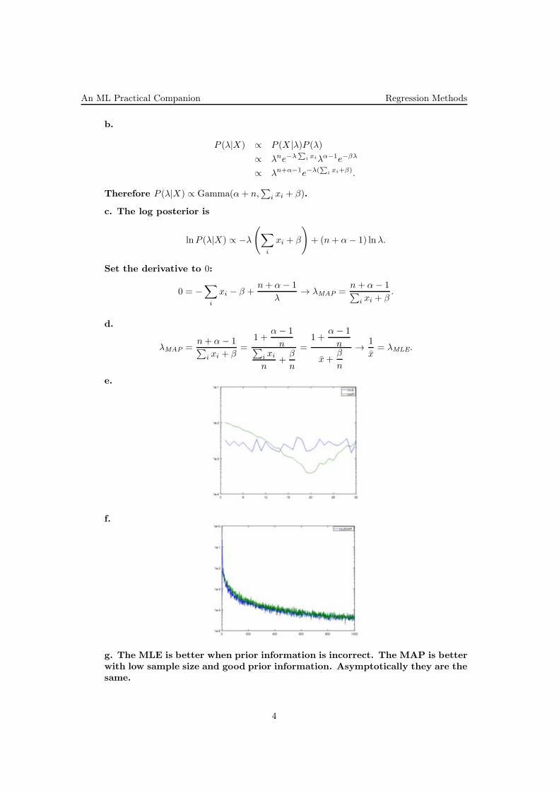
e. Let’s perform an experiment in the above setting. Generate n = 20 randomvariables drawn from Exp(λ = 0.2). Fix α = 100 and vary r over the range(1, 30) using a stepsize of 1. Compute the corresponding MLE and MAPestimates for λ. For each r, repeat this process 50 times and compute themean squared error of both estimates compared against the true value. Plotthe mean squared error as a function of r. (Note: Octave parameterizes theExponential distribution with θ = 1/λ.)
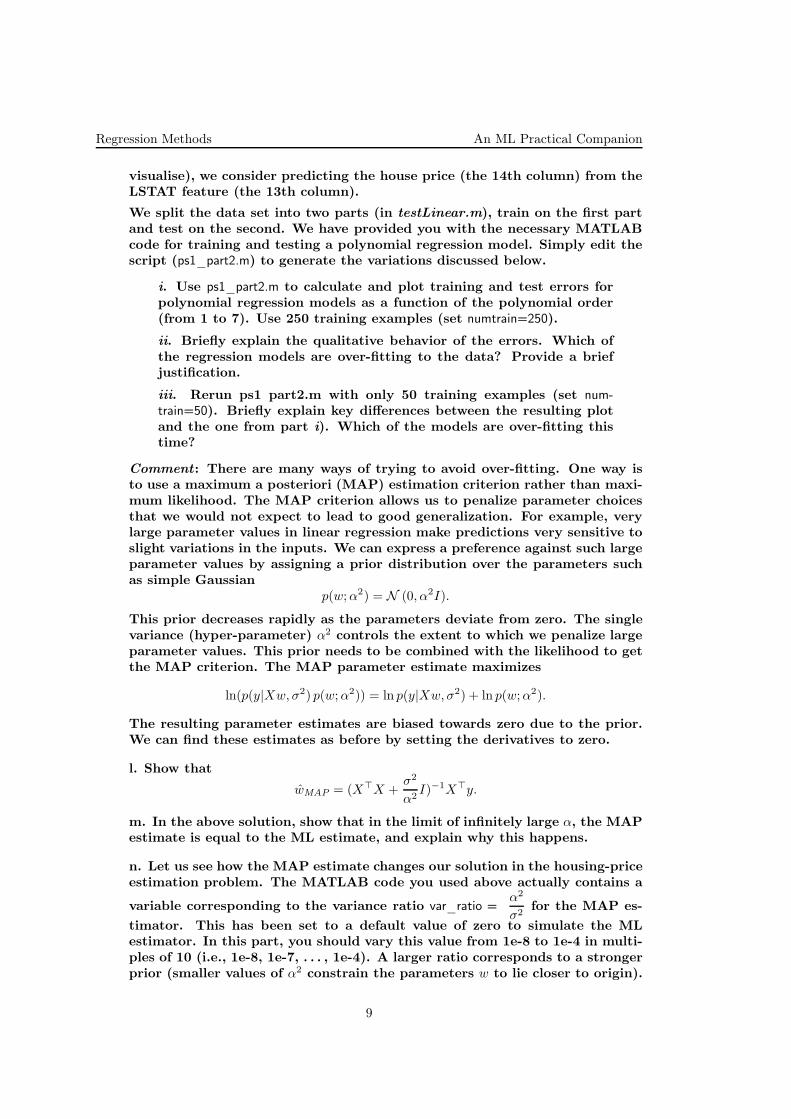
f. Now, fix (r, α) = (30, 100) and vary n up to 1000. Plot the MSE for each n ofthe corresponding estimates.
g. Under what conditions is the MLE estimator better? Under what condi-tions is the MAP estimator better? Explain the behavior in the two aboveplots.
Răspuns:
a. The log likelihood is
ℓ(λ) =∑
i
lnλ− λxi = nlogλ− λ∑
i
xi
Set the derivative to 0:
n
λ−∑
i
xi = 0⇒ λMLE =1
x.
This is biased.
3
An ML Practical Companion Regression Methods
b.
P (λ|X) ∝ P (X |λ)P (λ)
∝ λne−λ∑
i xiλα−1e−βλ
∝ λn+α−1e−λ(∑
ixi+β).
Therefore P (λ|X) ∝ Gamma(α+ n,∑
i xi + β).
c. The log posterior is
lnP (λ|X) ∝ −λ(
∑
i
xi + β
)
+ (n+ α− 1) lnλ.
Set the derivative to 0:
0 = −∑
i
xi − β +n+ α− 1
λ→ λMAP =
n+ α− 1∑
i xi + β.
d.
λMAP =n+ α− 1∑
i xi + β=
1 +α− 1
n∑
i xi
n+
β
n
=1 +
α− 1
n
x+β
n
→ 1
x= λMLE.
e.
f.
g. The MLE is better when prior information is incorrect. The MAP is betterwith low sample size and good prior information. Asymptotically they are thesame.
4

Regression Methods An ML Practical Companion
3. (Distribuţia binomială: estimarea parametrului în sens MLE,xxx folosind metoda lui Newton;xxx distribuţia Gamma: estimarea parametrilor în sens MLE,xxx folosind metoda gradientului şi metoda lui Newton)
• CMU, 2008 spring, Tom Mitchell, HW2, pr. 1.2xxx • CMU, 2015 fall, A. Smola, B. Poczos, HW1, pr. 1.2.c
a. For the binomial sampling function, pdf f(x) = Cxnp
x(1−p)n−x, find the MLEusing the Newton-Raphson method, starting with an estimate θ0 = 0.1, n = 100,x = 8. Show the resulting θj until it reaches convergence (θj+1−θj < .01). (Notethat the binomial pdf may be calculated analytically -– you may use this tocheck your answer.)
b. Note: For this [part of the] exercise, please make use of the digamma andtrigamma functions. You can find the digamma and trigamma functions inany scientific computing package (e.g. Octave, Matlab, Python...).
Inside the handout, the estimators.mat file contains a vector drawn from aGamma distribution. Run your implementation of gradient descent and New-ton’s method — for the later, see the ex. ?? in our exercise book — to obtainthe MLE estimators for this distribution. Create a plot showing the conver-gence of the two above methods. How do they compare? Which took moreiterations? Lastly, provide the actual estimated values obtained.
Solution:
a.
b. You should have gotten α ≈ 4, β ≈ 0.5.
5

An ML Practical Companion Regression Methods
4. (Distribuţia categorială:: estimarea parametrilorxxx în sens MLE şi respectiv în sens MAP,xxx folosind ca distribuţie a priori distribuţia Dirichlet;xxx testare la clasificare de documente)
• MIT, 2011 fall, Leslie Kaelbling, HW3, pr. 2
6

Regression Methods An ML Practical Companion
5. (Linear, polynomial, regularized (L2), and kernelized regression:xxx application on a [UCI ML Repository] datasetxxx for housing prices in Boston area)
• · MIT, 2001 fall, Tommi Jaakkola, HW1, pr. 1xxx MIT, 2004 fall, Tommi Jaakkola, HW1, pr. 3xxx MIT, 2006 fall, Tommi Jaakkola, HW2, pr. 2.d
A. Here we will be using a regression method to predict housing prices insuburbs of Boston. You’ll find the data in the file housing.data. Informationabout the data, including the column interpretation can be found in the filehousing.names. These files are taken from the UCI Machine Learning Repositoryhttps://archive.ics.uci.edu/ml/datasets.html.
We will predict the median house value (the 14th, and last, column of thedata) based on the other columns.
a. First, we will use a linear regression model to predict the house values,using squared-error as the criterion to minimize. In other words y = f(x; w) =
w0 +∑13
i=1 wixi, where w = argminw∑n
t=1(yt − f(xt;w))2; here yt are the house
values, xt are input vectors, and n is the number of training examples.
Write the following MATLAB functions (these should be simple functions tocode in MATLAB):
• A function that takes as input weights w and a set of input vectorsxtt=1,...,n, and returns the predicted output values ytt=1,...,n.
• A function that takes as input training input vectors and output values,and return the optimal weight vector w.
• A function that takes as input a training set of input vectors and outputvalues, and a test set input vectors, and output values, and returns themean training error (i.e., average squared-error over all training samples)and mean test error.
b. To test our linear regression model, we will use part of the data set as atraining set, and the rest as a test set. For each training set size, use the firstlines of the data file as a training set, and the remaining lines as a test set.Write a MATLAB function that takes as input the complete data set, and thedesired training set size, and returns the mean training and test errors.
Turn in the mean squared training and test errors for each of the followingtraining set sizes: 10, 50, 100, 200, 300, 400.
(Quick validation: For a sample size of 100, we got a mean training error of4.15 and a mean test error of 1328.)
c. What condition must hold for the training input vectors so that the trainingerror will be zero for any set of output values?
d. Do the training and test errors tend to increase or decrease as the trainingset size increases? Why? Try some other training set sizes to see that this isonly a tendency, and sometimes the change is in the different direction.
e. We will now move on to polynomial regression. We will predict the housevalues using a function of the form:
f(x;w) = w0 +
13∑
i=1
m∑
d=1
wi,d xdi ,
7

An ML Practical Companion Regression Methods
where again, the weights w are chosen so as to minimize the mean squarederror of the training set. Think about why we also include all lower orderpolynomial terms up to the highest order rather than just the highest ones.
Note that we only use features which are powers of a single input feature.We do so mostly in order to simplify the problem. In most cases, it is morebeneficial to use features which are products of different input features, andperhaps also their powers.
Think of why such features are usually more powerful.
Write a version of your MATLAB function from section b that takes as inputalso a maximal degree m and returns the training and test error under sucha polynomial regression model.
NOTE : When the degree is high, some of the features will have extremelyhigh values, while others will have very low values. This causes severe nume-ric precision problems with matrix inversion, and yields wrong answers. Toovercome this problem, you will have to appropriately scale each feature xd
i
included in the regression model, to bring all features to roughly the samemagnitude. Be sure to use the same scaling for the training and test sets.For example, divide each feature by the maximum absolute value of the fe-ature, among all training and test examples. (MATLAB matrix and vectoroperations can be very useful for doing such scaling operations easily.)
f.
g. For a training set size of 400, turn in the mean squared training and testerrors for maximal degrees of zero through ten.
(Quick validation: for maximal degree two, we got a training error of 14.5 anda test error of 32.8).
h. Explain the qualitative behavior of the test error as a function of thepolynomial degree. Which degree seems to be the best choice?
i. Prove (in two sentences) that the training error is monotonically decreasingwith the maximal degree m. That is, that the training error using a higherdegree and the same training set, is necessarily less then or equal to thetraining error using a lower degree.
j. We claim that if there is at least one feature (component of the inputvector x) with no repeated values in the training set, then the training errorwill approach zero as the polynomial degree increases. Why is this true?
B. In this [part of the] problem, we explore the behavior of polynomial re-gression methods when only a small amount of training data is available.
...
We will begin by using a maximum likelihood estimation criterion for theparameters w that reduces to least squares fitting.
k. Consider a simple 1D regression problem. The data in housing.data providesinformation of how 13 different factors affect house price in the Boston area.(Each column of data represents a different factor, and is described in briefin the file housing.names.) To simplify matters (and make the problem easier to
8
Regression Methods An ML Practical Companion
visualise), we consider predicting the house price (the 14th column) from theLSTAT feature (the 13th column).
We split the data set into two parts (in testLinear.m), train on the first partand test on the second. We have provided you with the necessary MATLABcode for training and testing a polynomial regression model. Simply edit thescript (ps1_part2.m) to generate the variations discussed below.
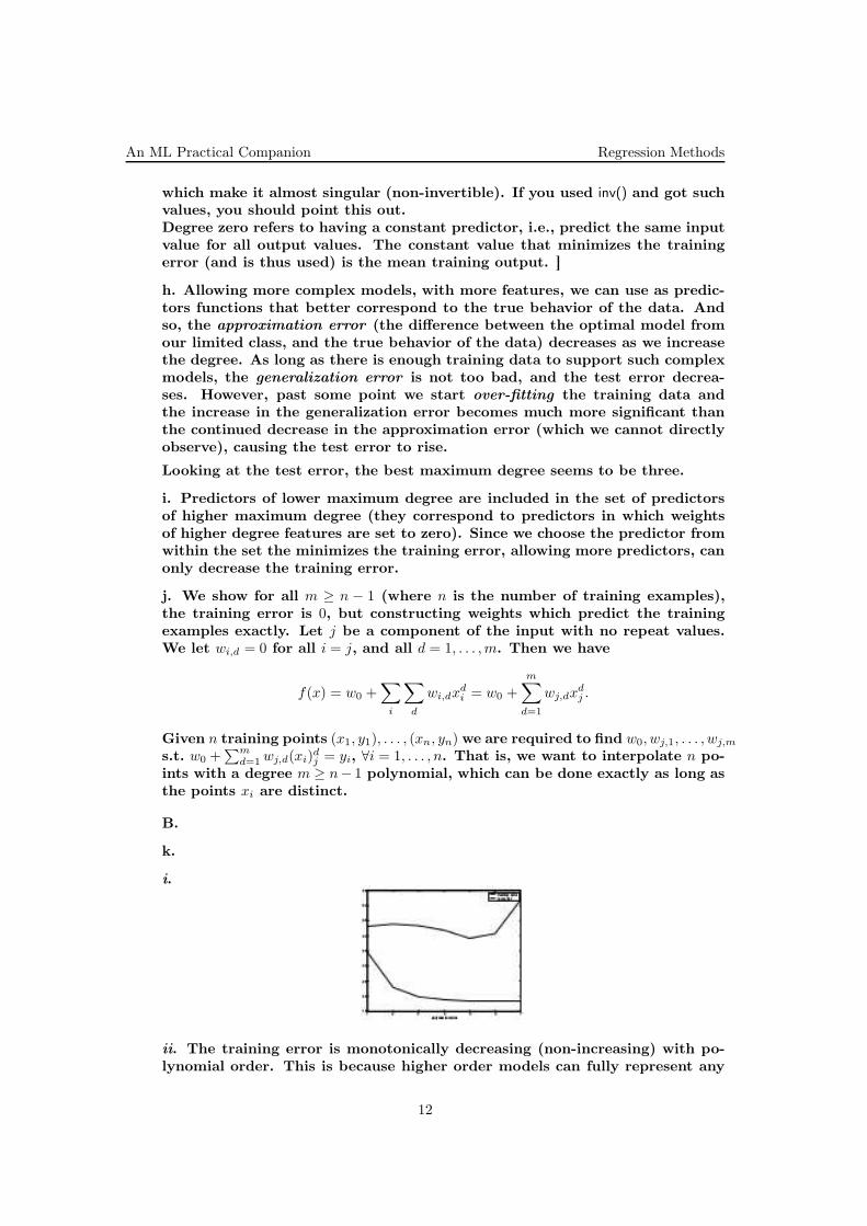
i. Use ps1_part2.m to calculate and plot training and test errors forpolynomial regression models as a function of the polynomial order(from 1 to 7). Use 250 training examples (set numtrain=250).
ii. Briefly explain the qualitative behavior of the errors. Which ofthe regression models are over-fitting to the data? Provide a briefjustification.
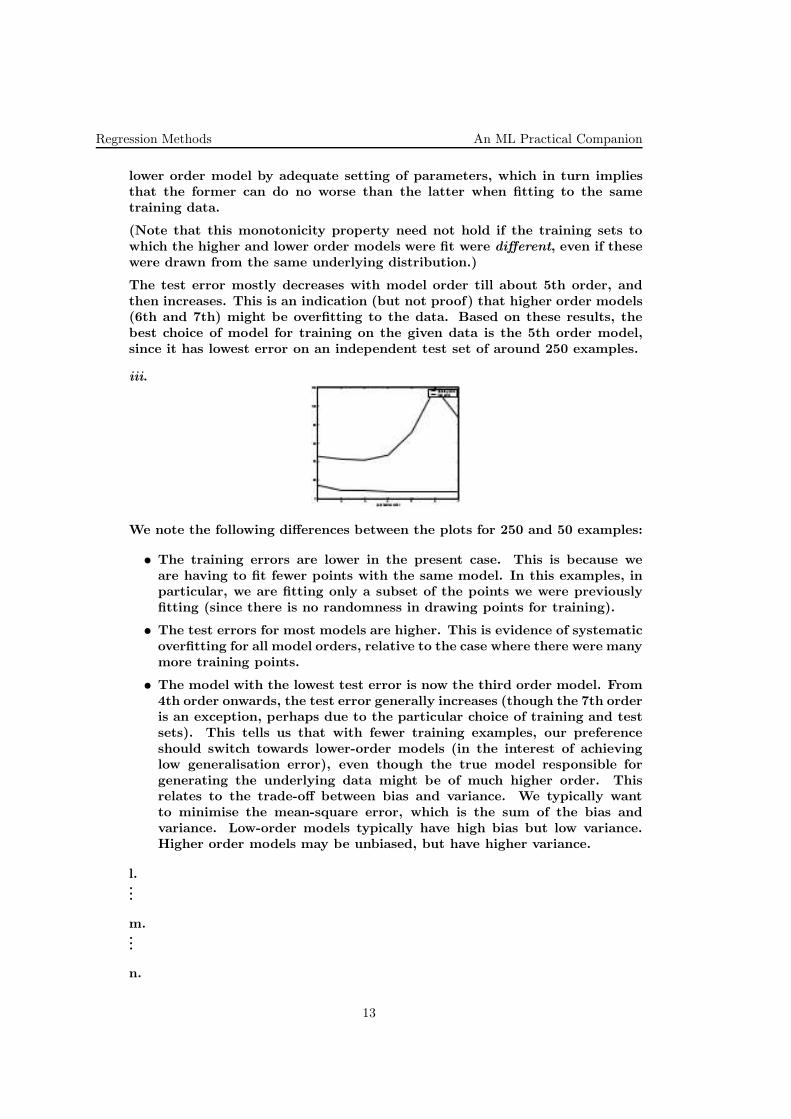
iii. Rerun ps1 part2.m with only 50 training examples (set num-train=50). Briefly explain key differences between the resulting plotand the one from part i). Which of the models are over-fitting thistime?
Comment : There are many ways of trying to avoid over-fitting. One way isto use a maximum a posteriori (MAP) estimation criterion rather than maxi-mum likelihood. The MAP criterion allows us to penalize parameter choicesthat we would not expect to lead to good generalization. For example, verylarge parameter values in linear regression make predictions very sensitive toslight variations in the inputs. We can express a preference against such largeparameter values by assigning a prior distribution over the parameters suchas simple Gaussian
p(w;α2) = N (0, α2I).
This prior decreases rapidly as the parameters deviate from zero. The singlevariance (hyper-parameter) α2 controls the extent to which we penalize largeparameter values. This prior needs to be combined with the likelihood to getthe MAP criterion. The MAP parameter estimate maximizes
ln(p(y|Xw, σ2) p(w;α2)) = ln p(y|Xw, σ2) + ln p(w;α2).
The resulting parameter estimates are biased towards zero due to the prior.We can find these estimates as before by setting the derivatives to zero.
l. Show that
wMAP = (X⊤X +σ2
α2I)−1X⊤y.
m. In the above solution, show that in the limit of infinitely large α, the MAPestimate is equal to the ML estimate, and explain why this happens.
n. Let us see how the MAP estimate changes our solution in the housing-priceestimation problem. The MATLAB code you used above actually contains a
variable corresponding to the variance ratio var_ratio =α2
σ2for the MAP es-
timator. This has been set to a default value of zero to simulate the MLestimator. In this part, you should vary this value from 1e-8 to 1e-4 in multi-ples of 10 (i.e., 1e-8, 1e-7, . . . , 1e-4). A larger ratio corresponds to a strongerprior (smaller values of α2 constrain the parameters w to lie closer to origin).
9

An ML Practical Companion Regression Methods
iv. Plot the training and test errors as a function of the polynomialorder using the above 5 MAP estimators and 250 and 50 trainingpoints.
v. Describe how the prior affects the estimation results.
C. Implement the kernel linear regression method (described in MIT, 2006fall, Tommi Jaakkola, HW2, pr. 2.a-c / Estimp-56 / Estimp-72) for λ > 0. Weare interested in exploring how the regularization parameter λ ≥ 0 affects thesolution when the kernel function is the radial basis kernel
K(x, x′) = exp
(
−β
2‖x− x′‖2
)
, β > 0.
We have provided training and test data as well as helpful MATLAB scriptsin hw2/prob2. You should only need to complete the relevant lines in run prob2script. The data pertains to the problem of predicting Boston housing pricesbased on various indicators (normalized). Evaluate and plot the training andtest errors (mean squared errors) as a function of λ in the range λ ∈ (0, 1). Useβ = 0.05. Explain the qualitative behavior of the two curves.
Solution:
A.
a.
b. First to read the data (ignoring column four):
» data = load(’housing.data’);» x = data(:,[1:3 5:13]);» y = data(:,14);
To get the training and test errors for training set of size s, we invoke thefollowing MATLAB command:
» [trainE,testE] = testLinear(x,y,s)
Here are the errors I got:
training size training error test error10 6.27× 10⁻²⁶ 1.05× 10⁵
50 3.437 24253100 4.150 1328200 9.538 316.1300 9.661 381.6400 22.52 41.23
[ Note that for a training size of ten, the training error should have beenzero. The very low, but still non-zero, error is a result of limited precision ofthe calculations, and is not a problem. Furthermore, with only ten trainingexamples, the optimal regression weights are not uniquely defined. There is afour dimensional linear subspace of weight vectors that all yield zero trainingerror. The test error above (for a training size of ten) represents an 2arbitrarychoice of weights from this subspace (implicitly made by the pinv() function).Using different, equally optimal, weights would yield different test errors. ]
10

Regression Methods An ML Practical Companion
c. The training error will be zero if the input vectors are linearly independent.More precisely, since we are allowing an affine term w0, it is enough thatthe input vectors with an additional term always equal to one, are linearlyindependent. Let X be the matrix of input vectors, with additional ‘one’terms, y any output vector, and w a possible weight vector. If the inputs arelinearly independent, Xw = y always has a solution, and the weights w lead tozero training error.
[ Note that if X is a square matrix with linearly independent rows, than itis invertible, and Xw = y has a unique solution. But even if X is not squarematrix, but its rows are still linearly independent (this can only happen ifthere are less rows then columns, i.e., less features then training examples),then there are solutions to Xw = y, which do not determine w uniquely, butstill yield zero training error (as in the case of a sample size of ten above). ]
d. The training error tends to increase. As more examples have to be fitted,it becomes harder to ’hit’, or even come close, to all of them.
The test error tends to decrease. As we take into account more exampleswhen training, we have more information, and can come up with a model thatbetter resembles the true behavior. More training examples lead to bettergeneralization.
e. We will use the following functions, on top of those from question b:
function xx = degexpand(x, deg)function [trainE, testE] = testPoly(x, y, numtrain, deg)
f....
g. To get the training and test errors for maximum degree d, we invoke thefollowing MATLAB command:
» [trainE,testE] = testPoly(x,y,400,d)
Here are the errors I got:
degree training error test error0 83.8070 102.22661 22.5196 41.22852 14.8128 32.83323 12.9628 31.78804 10.8684 52625 9.4376 50676 7.2293 4.8562× 10⁷
7 6.7436 1.5110× 10⁶
8 5.9908 3.0157× 10⁹
9 5.4299 7.8748× 10¹⁰
10 4.3867 5.2349× 10¹³
[ These results were obtained using pinv(). Using different operations, althoughtheoretically equivalent, might produce different results for higher degrees. Inany case, using any of the suggested methods above, the errors should matchthe above table at least up to degree five. Beyond that, using inv() startsproducing unreasonable results due to extremely small values in the matrix,
11
An ML Practical Companion Regression Methods
which make it almost singular (non-invertible). If you used inv() and got suchvalues, you should point this out.Degree zero refers to having a constant predictor, i.e., predict the same inputvalue for all output values. The constant value that minimizes the trainingerror (and is thus used) is the mean training output. ]
h. Allowing more complex models, with more features, we can use as predic-tors functions that better correspond to the true behavior of the data. Andso, the approximation error (the difference between the optimal model fromour limited class, and the true behavior of the data) decreases as we increasethe degree. As long as there is enough training data to support such complexmodels, the generalization error is not too bad, and the test error decrea-ses. However, past some point we start over-fitting the training data andthe increase in the generalization error becomes much more significant thanthe continued decrease in the approximation error (which we cannot directlyobserve), causing the test error to rise.
Looking at the test error, the best maximum degree seems to be three.
i. Predictors of lower maximum degree are included in the set of predictorsof higher maximum degree (they correspond to predictors in which weightsof higher degree features are set to zero). Since we choose the predictor fromwithin the set the minimizes the training error, allowing more predictors, canonly decrease the training error.
j. We show for all m ≥ n − 1 (where n is the number of training examples),the training error is 0, but constructing weights which predict the trainingexamples exactly. Let j be a component of the input with no repeat values.We let wi,d = 0 for all i = j, and all d = 1, . . . ,m. Then we have
f(x) = w0 +∑
i
∑
d
wi,dxdi = w0 +
m∑
d=1
wj,dxdj .
Given n training points (x1, y1), . . . , (xn, yn) we are required to find w0, wj,1, . . . , wj,m
s.t. w0 +∑m
d=1wj,d(xi)dj = yi, ∀i = 1, . . . , n. That is, we want to interpolate n po-
ints with a degree m ≥ n− 1 polynomial, which can be done exactly as long asthe points xi are distinct.
B.
k.
i.
ii. The training error is monotonically decreasing (non-increasing) with po-lynomial order. This is because higher order models can fully represent any
12
Regression Methods An ML Practical Companion
lower order model by adequate setting of parameters, which in turn impliesthat the former can do no worse than the latter when fitting to the sametraining data.
(Note that this monotonicity property need not hold if the training sets towhich the higher and lower order models were fit were different, even if thesewere drawn from the same underlying distribution.)
The test error mostly decreases with model order till about 5th order, andthen increases. This is an indication (but not proof) that higher order models(6th and 7th) might be overfitting to the data. Based on these results, thebest choice of model for training on the given data is the 5th order model,since it has lowest error on an independent test set of around 250 examples.
iii.
We note the following differences between the plots for 250 and 50 examples:
• The training errors are lower in the present case. This is because weare having to fit fewer points with the same model. In this examples, inparticular, we are fitting only a subset of the points we were previouslyfitting (since there is no randomness in drawing points for training).
• The test errors for most models are higher. This is evidence of systematicoverfitting for all model orders, relative to the case where there were manymore training points.
• The model with the lowest test error is now the third order model. From4th order onwards, the test error generally increases (though the 7th orderis an exception, perhaps due to the particular choice of training and testsets). This tells us that with fewer training examples, our preferenceshould switch towards lower-order models (in the interest of achievinglow generalisation error), even though the true model responsible forgenerating the underlying data might be of much higher order. Thisrelates to the trade-off between bias and variance. We typically wantto minimise the mean-square error, which is the sum of the bias andvariance. Low-order models typically have high bias but low variance.Higher order models may be unbiased, but have higher variance.
l....
m....
n.
13
An ML Practical Companion Regression Methods
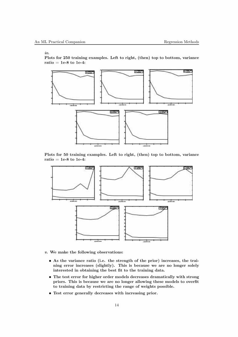
iv.Plots for 250 training examples. Left to right, (then) top to bottom, varianceratio = 1e-8 to 1e-4:
Plots for 50 training examples. Left to right, (then) top to bottom, varianceratio = 1e-8 to 1e-4:
v. We make the following observations:
• As the variance ratio (i.e. the strength of the prior) increases, the trai-ning error increases (slightly). This is because we are no longer solelyinterested in obtaining the best fit to the training data.
• The test error for higher order models decreases dramatically with strongpriors. This is because we are no longer allowing these models to overfitto training data by restricting the range of weights possible.
• Test error generally decreases with increasing prior.
14
Regression Methods An ML Practical Companion
• As a consequence of the above two points, the best model changes slightlywith increasing prior in the direction of more complex models.
• For 50 training samples, the difference in test error between ML andMAP is more significant than with 250 training examples. This is becauseoverfitting is a more serious problem in the former case.
C. Sample code for this problem is shown below:
Ntrain = size(Xtrain,1);Ntest = size(Xtest,1);
for i=1:length(lambda),lmb = lambda(i);alpha = lmb * ((lmb*eye(Ntrain) + K)∧-1) * Ytrain;Atrain = (1/lmb) * repmat( alpha’, Ntrain, 1);yhat_train = sum(Atrain.*K,2);Atest = (1/lmb) * repmat( alpha’, Ntest, 1);yhat_test = sum(Atest.*(Ktrain_test’), 2);E(i,:) = [mean((yhat_train-Ytrain).∧2),mean((yhat_test-Ytest).∧2)];
end;
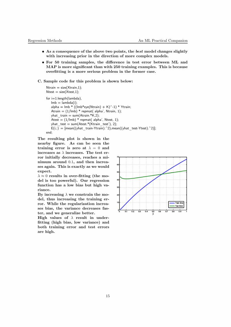
The resulting plot is shown in thenearby figure. As can be seen thetraining error is zero at λ = 0 andincreases as λ increases. The test er-ror initially decreases, reaches a mi-nimum around 0.1, and then increa-ses again. This is exactly as we wouldexpect.λ ≈ 0 results in over-fitting (the mo-del is too powerful). Our regressionfunction has a low bias but high va-riance.By increasing λ we constrain the mo-del, thus increasing the training er-ror. While the regularization increa-ses bias, the variance decreases fas-ter, and we generalize better.High values of λ result in under-fitting (high bias, low variance) andboth training error and test errorsare high.
15
An ML Practical Companion Regression Methods
6. (Regresia liniară local-ponderată (ne-regularizată))
• Stanford, 2011 fall, Andrew Ng, HW1, pr. 2.d
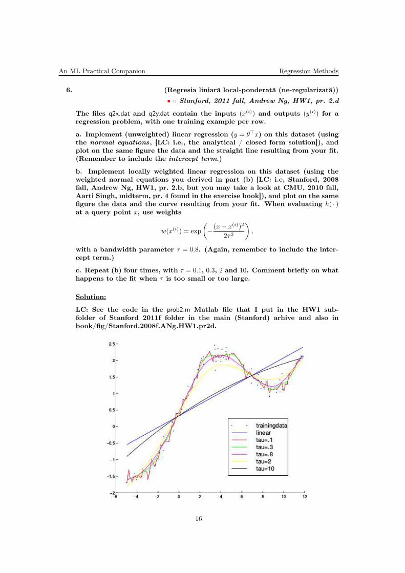
The files q2x.dat and q2y.dat contain the inputs (x(i)) and outputs (y(i)) for aregression problem, with one training example per row.
a. Implement (unweighted) linear regression (y = θ⊤x) on this dataset (usingthe normal equations, [LC: i.e., the analytical / closed form solution]), andplot on the same figure the data and the straight line resulting from your fit.(Remember to include the intercept term.)
b. Implement locally weighted linear regression on this dataset (using theweighted normal equations you derived in part (b) [LC: i.e, Stanford, 2008fall, Andrew Ng, HW1, pr. 2.b, but you may take a look at CMU, 2010 fall,Aarti Singh, midterm, pr. 4 found in the exercise book]), and plot on the samefigure the data and the curve resulting from your fit. When evaluating h( · )at a query point x, use weights
w(x(i)) = exp
(
− (x− x(i))2
2τ2
)
,
with a bandwidth parameter τ = 0.8. (Again, remember to include the inter-cept term.)
c. Repeat (b) four times, with τ = 0.1, 0.3, 2 and 10. Comment briefly on whathappens to the fit when τ is too small or too large.
Solution:
LC: See the code in the prob2.m Matlab file that I put in the HW1 sub-folder of Stanford 2011f folder in the main (Stanford) arhive and also inbook/fig/Stanford.2008f.ANg.HW1.pr2d.
16

Regression Methods An ML Practical Companion
(Plotted in color where available.)
For small bandwidth parameter τ , the fitting is dominated by the closest bytraining samples. The smaller the bandwidth, the less training samples thatare actually taken into account when doing the regression, and the regressionresults thus become very susceptible to noise in those few training samples.
For larger τ , we have enough training samples to reliably fit straight lines,unfortunately a straight line is not the right model for these data, so we alsoget a bad fit for large bandwidths.
17

An ML Practical Companion Regression Methods
7. ([Weighted] Linear Regression applied toxxx predicting the needed quatity of insulin,xxx starting from the sugar level in the patient’s blood)
• CMU, 2009 spring, Ziv Bar-Joseph, HW1, pr. 4
An automated insulin injector needs to calculate how much insulin it shouldinject into a patient based on the patient’s blood sugar level. Let us formulatethis as a linear regression problem as follows: let yi be the dependent predictedvariable (blood sugar level), and let β0, β1 and β2 be the unknown coefficientsof the regression function. Thus, yi = β0 + β1xi + β2x
2i , and we can formulate
the problem of finding the unknown βnot.= (β0, β1, β2) as:
β = (X⊤X)−1X⊤y.
See data2.txt (posted on website) for data based on the above scenario withspace separated fields conforming to:bloodsugarlevel insulinedose weightage
The purpose of the weightage field will be made clear in part c.
a. Write code in Matlab to estimate the regression coefficients given thedataset consisting of pairs of independent and dependent variables. Generatea space separated file with the estimated parameters from the entire datasetby writing out all the parameter.
b. Write code in Matlab to perform inference by predicting the insulin dosagegiven the blood sugar level based on training data using a leave one out crossvalidation scheme. Generate a space separated file with the predicted dosagesin order. The predicted dosages:
c. However, it has been found that one group of patients are twice as sensitiveto the insuline dosage than the other. In the training data, these particularpatients are given a weightage of 2, while the others are given a weightage
of 1. Is your goodness of fit function flexible enough to incorporate thisinformation?
d. Show how to formulate the regression function, and correspondingly cal-culate the coefficients of regression under this new scenario, by incorporatingthe given weights.
e. Code up this variant of regressional analysis. Write out the new coefficientsof regression you obtain by using the whole dataset as training data.
Solution:
a. The betas, in order:−74.3825 13.4215 1.1941
b.1417.0177 1501.4423 1966.3563 2833.7942 2953.4532 3075.472 3199.8566 3326.96633456.4704 5038.3777 5196.6767 5357.0094 7091.8113 7278.2709 7467.3604 7658.52567852.0808 9703.9748 9921.8604 10142.5438 10365.8512 12498.2968 12749.6202 13003.941798.3745 1869.1966 2024.7112 2265.6988 2392.0227 2756.1588 3915.9302 4004.4654878.0057 5094.3282 6217.981 6485.8542 6544.4688 6805.7564 7073.8455 7207.50327285.3657 9393.5129 9515.9043 9704.0029 10060.5539 12037.6304 12361.3586 12903.5394
18

Regression Methods An ML Practical Companion
c. Since we need to weigh each point differently, out current goodness of fitfunction is unable to work in this scenario. However, since the weights for thisspecific dataset are 1 and 2, we may just use the old formalism and doublethe data items with weightage 2. The changed formalism which enables us toassign weights of any precision to the data sample is shown below.
d. Let:
y = Xβ
y = (y1, y2, . . . , yn)⊤
β = (β1, β2, . . . , βm)⊤
Xi,1 = 1
Xi,j+1 = xi,j
Let us define the weight matrix as:Ωi,i =
√wi
Ωi,j = 0 (for i 6= j)So, Ωy = ΩXβ.
To minimize the weighted square error, we have to take the derivative withrespect to β:
∂
∂β((Ωy − ΩXβ)⊤(Ωy − ΩXβ))
=∂
∂β((Ωy)⊤(Ωy)− 2(Ωy)⊤(ΩXβ) + (ΩXβ)⊤(ΩXβ)
=∂
∂β((Ωy)⊤(Ωy)− 2(Ωy)⊤(ΩXβ) + β⊤X⊤Ω⊤ΩXβ
Therefore
∂
∂β((Ωy − ΩXβ)⊤(Ωy − ΩXβ)) = 0
⇔ 0− 2((Ωy)⊤(ΩX))⊤ + 2X⊤Ω⊤ΩXβ = 0
⇔ β = (X⊤Ω⊤ΩX)−1X⊤Ω⊤Ωy
e. The new beta coefficients are in order:−57.808 13.821 1.199
19
An ML Practical Companion Regression Methods
8. (Linear [Ridge] regression applied toxxx predicting the level of PSA in the prostate gland,xxx using a set of medical test results)
• ⋆ ⋆ CMU, 2009 fall, Geoff Gordon, HW3, pr. 3
The linear regression method is widely used in the medical domain. In thisquestion you will work on a prostate cancer data from a study by Stamey etal.888 You can download the data from . . . .
Your task is to predict the level of prostate-specific antigen (PSA) using a setof medical test results. PSA is a protein produced by the cells of the prostategland. High levels of PSA often indicate the presence of prostate cancer orother prostate disorders.
The attributes are several clinical measurements on men who have prostatecancer. There are 8 attributes: log cancer volume lcavol, log prostate weight(lweight), log of the amount of benign prostatic hyperplasia (lbph), seminalvesicle invasion (svi), age, log of capsular penetration (lcp), Gleason score(gleason), and percent of Gleason scores of 4 or 5 (pgg45). svi and gleason
are categorical, that is they take values either 1 or 0; others are real-valued.We will refer to these attributes as A1 = lcavol, A2 = lweight, A3 = age, A4
= lbph, A5 = svi, A6 = lcp, A7 = gleason, A8 = pgg45.
Each row of the input file describes one data point: the first column is theindex of the data point, the following eight columns are attributes, and thetenth column gives the log PSA level lpsa, the response variable we are in-terested in. We already randomized the data and split it into three partscorresponding to training, validation and test sets. The last column of the fileindicates whether the data point belongs to the training set, validation setor test set, indicated by ‘1’ for training, ‘2’ for validation and ‘3’ for testing.The training data includes 57 examples; validation and test sets contain 20examples each.
Inspecting the Data
a. Calculate the correlation matrix of the 8 attributes and report it in a table.The table should be 8-by-8. You can use Matlab functions.
b. Report the top 2 pairs of attributes that show the highest pairwise positivecorrelation and the top 2 pairs of attributes that show the highest pairwisenegative correlation.
Solving the Linear Regression Problem
You will now try to find several models in order to predict the lpsa levels.The linear regression model is
Y = f(X) + ǫ
where ǫ is a Gaussian noise variable, and
f(X) =
p∑
j=0
wjφj(X)
888Stamey TA, Kabalin JN, McNeal JE et al. Prostate specific antigen in the diagnosis and treatment of theprostate. II. Radical prostatectomy treated patients. J Urol 1989;141:107683.
20

Regression Methods An ML Practical Companion
where p is the number of basis functions (features), φj is the jth basis function,and wj is the weight we wish to learn for the jth basis function. In the modelsbelow, we will always assume that φ0(X) = 1 represents the intercept term.
c. Write a Matlab function that takes the data matrix Φ and the columnvector of responses y as an input and produces the least squares fit w as theoutput (refer to the lecture notes for the calculation of w).
d. You will create the following three models. Note that before solving eachregression problem below, you should scale each feature vector to have azero mean and unit variance. Don’t forget to include the intercept column,φ0(X) = 1, after scaling the other features. Notice that since you shifted theattributes to have zero mean, in your solutions, the intercept term will be themean of the response variable.
• Model1: Features are equal to input attributes, with the addition of a con-stant feature φ0. That is, φ0(X) = 1, φ1(X) = A1, . . . , φ8(X) = A8. Solve thelinear regression problem and report the resulting feature weights. Discusswhat it means for a feature to have a large negative weight, a large positiveweight, or a small weight. Would you be able to comment on the weights, ifyou had not scaled the predictors to have the same variance? Report meansquared error (MSE) on the training and validation data.
• Model2: Include additional features corresponding to pairwise products ofthe first six of the original attributes,889 i.e., φ9(X) = A1·A2, . . . , φ13(X) = A1·A6,φ15(X) = A2 · A3, . . . , φ23(X) = A5 · A6. First compute the features accordingto the formulas above using the unnormalized values, then shift and scale thenew features to have zero mean and unit variance and add the column for theintercept term φ0(X) = 1. Report the five features whose weights achieved thelargest absolute values.
• Model3: Starting with the results of Model1, drop the four features withthe lowest weights (in absolute values). Build a new model using only theremaining features. Report the resulting weights.
e. Make two bar charts, the first to compare the training errors of the threemodels, the second to compare the validation errors of the three models.Which model achieves the best performance on the training data? Whichmodel achieves the best performance on the validation data? Comment ondifferences between training and validation errors for individual models.
f. Which of the models would you use for predicting the response variable?Explain.
Ridge Regression
For this question you will start with Model2 and employ regularization on it.
g. Write a Matlab function to solve Ridge regression. The function should takethe data matrix Φ, the column vector of responses y, and the regularizationparameter λ as the inputs and produce the least squares fit w as the output(refer to the lecture notes for the calculation of w). Do not penalize w0, the
889These features are also called interactions, because they attempt to account for the effect of two attributesbeing simultaneously high or simultaneously low.
21

An ML Practical Companion Regression Methods
intercept term. (You can achieve this by replacing the first column of the λImatrix with zeros.)
h. You will create a plot exploring the effect of the regularization parameteron training and validation errors. The x-axis is the regularization parameter(on a log scale) and the y-axis is the mean squared error. Show two curves inthe same graph, one for the training error and one for the validation error.Starting with λ = 2−30, try 50 values: at each iteration increase λ by a factorof 2, so that for example the second iteration uses λ = 2−29. For each λ, youneed to train a new model.
i. What happens to the training error as the regularization parameter in-creases? What about the validation error? Explain the curve in terms ofoverfitting, bias and variance.
j. What is the λ that achieves the lowest validation error and what is thevalidation error at that point? Compare this validation error to the Model2validation error when no regularization was applied (you solved this in parte). How does w differ in the regularized and unregularized versions, i.e., whateffect did regularization have on the weights?
k. Is this validation error lower or higher than the validation error of themodel you chose in part f? Which one should be your final model?
l. Now that you have decided on your model (features and possibly the re-gularization parameter), combine your training and validation data to makea combined training set, train your model on this combined training set, andcalculate it on the test set. Report the training and test errors.
Solution:
a.
lcavol lweight age lbph svi lcp gleason pgg45 lpsa
lcavol 1.0000 0.2805 0.2249 0.0273 0.5388 0.6753 0.4324 0.4336 0.7344
lweight 0.2805 1.0000 0.3479 0.4422 0.1553 0.1645 0.0568 0.1073 0.4333
age 0.2249 0.3479 1.0000 0.3501 0.1176 0.1276 0.2688 0.2761 0.1695
lbph 0.0273 0.4422 0.3501 1.0000 -0.0858 -0.0069 0.0778 0.0784 0.1798
svi 0.5388 0.1553 0.1176 -0.0858 1.0000 0.6731 0.3204 0.4576 0.5662
lcp 0.6753 0.1645 0.1276 -0.0069 0.6731 1.0000 0.5148 0.6315 0.5488
gleason 0.4324 0.0568 0.2688 0.0778 0.3204 0.5148 1.0000 0.7519 0.3689
pgg45 0.4336 0.1073 0.2761 0.0784 0.4576 0.6315 0.7519 1.0000 0.4223
lpsa 0.7344 0.4333 0.1695 0.1798 0.5662 0.5488 0.3689 0.4223 1.0000
b. The top 2 pairs that show the highest pairwise positive correlation aregleason - ppg4 (0.7519) and lcavol -lcp (0.6731). Highest negative correlations:lbph - svi (-0.0858) and lph - lcp (-0.0070).
c. See below:
function what=lregress(Y,X)% least square solution to linear regression% X is the feature matrix% Y is the response variable vectorwhat=inv(X’*X)*X’*Y;end
d.
Model1:
22

Regression Methods An ML Practical Companion
the weight vector:w = [2.68265, 0.71796, 0.17843,−0.21235, 0.25752, 0.42998,−0.14179, 0.08745, 0.02928].Model2:The largest five absolute values in descending order:lweight*age, lpbh, lweight, age, age*lpbh.
Model3:The features with have the lowest absolute weights in Model1:pgg45, gleason, lcp, lweight.The resulting weights: w = [2.6827, 0.7164,−0.1735, 0.3441, 0.4095].
e.
1 2 30
0.1
0.2
0.3
0.4
0.5
0.6
0.7Training Error of the Three Models
Model ID
Tra
inin
g M
SE
1 2 30
0.2
0.4
0.6
0.8
1Validation Error of the Three Models
Model ID
Va
lida
tio
n M
SE
Model2 achieves the best performance on the training data, whereas Model1achieves the best performance on the validation data. Model2 suffer fromoverfitting, indicated by the very good training model but low validation error.Model3 seems to be too simple, it has a higher training and a higher validationerror compared to Model1. The features that are dropped are informative, asindicated by the lower training and validation errors.
f. Model1, since it achieves the best performance on the validation data.Model2 overfits, and Model3 is too simple.
g. See below:
function what = ridgeregress(Y,X,lambda)% X is the feature matrix% Y is the response vector% what are the estimated weightspenal = lambda*eye(size(X,2));penal(:,1) = 0;what = inv(X’*X+penal)*X’*Y;end
23
An ML Practical Companion Regression Methods
h.
−30 −20 −10 0 10 200.2
0.4
0.6
0.8
1
1.2
1.4
1.6
log2(lambda)
MS
E
training error
testing error
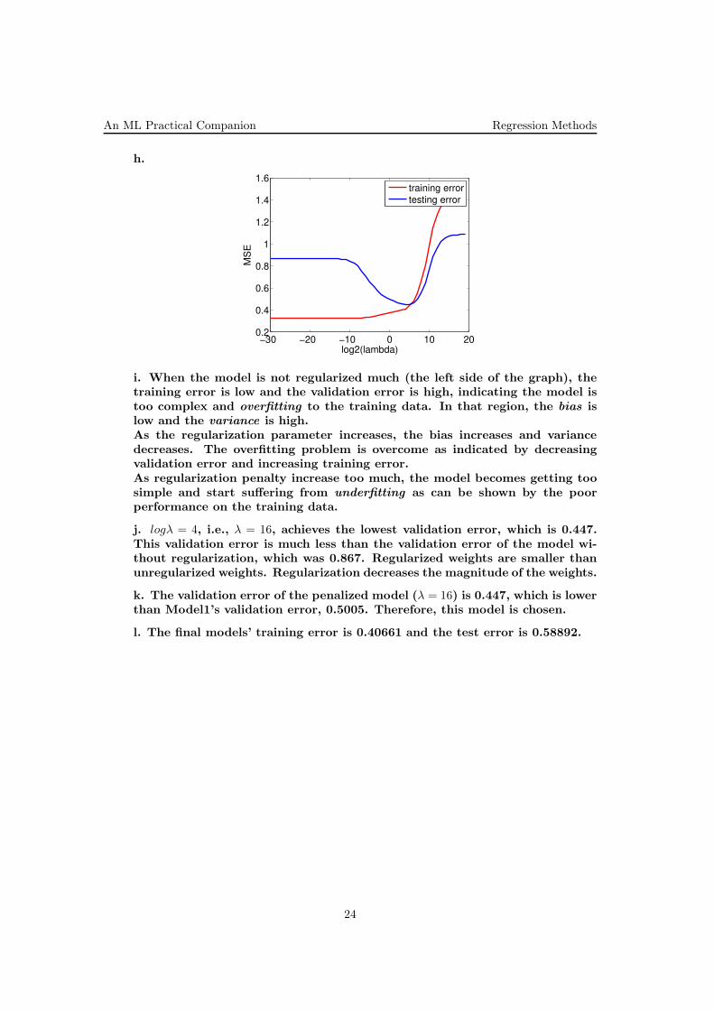
i. When the model is not regularized much (the left side of the graph), thetraining error is low and the validation error is high, indicating the model istoo complex and overfitting to the training data. In that region, the bias islow and the variance is high.As the regularization parameter increases, the bias increases and variancedecreases. The overfitting problem is overcome as indicated by decreasingvalidation error and increasing training error.As regularization penalty increase too much, the model becomes getting toosimple and start suffering from underfitting as can be shown by the poorperformance on the training data.
j. logλ = 4, i.e., λ = 16, achieves the lowest validation error, which is 0.447.This validation error is much less than the validation error of the model wi-thout regularization, which was 0.867. Regularized weights are smaller thanunregularized weights. Regularization decreases the magnitude of the weights.
k. The validation error of the penalized model (λ = 16) is 0.447, which is lowerthan Model1’s validation error, 0.5005. Therefore, this model is chosen.
l. The final models’ training error is 0.40661 and the test error is 0.58892.
24

Regression Methods An ML Practical Companion
9. (Linear weighted, unweighted, and functional regression:xxx application to denoising quasar spectra)
• · Stanford, 2017 fall, Andrew Ng, Dan Boneh, HW1, pr. 5xxx Stanford, 2016 fall, Andrew Ng, John Duchi, HW1, pr. 5
Solution:
25

An ML Practical Companion Regression Methods
10. (Linear regression with L1 / Lasso regularization:the coordinate descent method)
• ⋆ Stanford, 2007 fall, Andrew Ng, HW3, pr. 3.bc
Solution:
26

Regression Methods An ML Practical Companion
11. (Feature selection in the context of linear regressionxxx with L1 regularization:xxx the coordinate descent method)
• ⋆ MIT, 2003 fall, Tommi Jaakkola, HW4, pr. 1
Solution:
27
An ML Practical Companion Regression Methods
12. (Logistic regression with gradient ascent:xxx application on a synthetic dataset from R
2;xxx overfitting)
• CMU, 2015 spring, T. Mitchell, N. Balcan, HW4, pr. 2.c-i
In logistic regression, our goal is to learn a set of parameters by maximizingthe conditional log-likelihood of the data.
In this problem you will implement a logistic regression classifier and apply itto a two-class classification problem. In the archive, you will find one .m filefor each of the functions that you are asked to implement, along with a filecalled HW4Data.mat that contains the data for this problem. You can load thedata into Octave by executing load(”HW4Data.mat”) in the Octave interpreter.Make sure not to modify any of the function headers that are provided.
a. Implement a logistic regression classifier using gradient ascent — for theformulas and their calculation see ex. ?? in our exercise book890 — by fillingin the missing code for the following functions:
• Calculate the value of the objective function:obj = LR_CalcObj(XTrain,yTrain,wHat)
• Calculate the gradient:grad = LR_CalcGrad(XTrain,yTrain,wHat)
• Update the parameter value:wHat = LR_UpdateParams(wHat,grad,eta)
• Check whether gradient ascent has converged:hasConverged = LR_CheckConvg(oldObj,newObj,tol)
• Complete the implementation of gradient ascent:[wHat,objVals] = LR_GradientAscent(XTrain,yTrain)
• Predict the labels for a set of test examples:[yHat,numErrors] = LR_PredictLabels(XTest,yTest,wHat)
where the arguments and return values of each function are defined as follows:
• XTrain is an n × p dimensional matrix that contains one training instanceper row
• yTrain is an n × 1 dimensional vector containing the class labels for eachtraining instance
• wHat is a p+1× 1 dimensional vector containing the regression parameterestimates w0, w1, . . . , wp
• grad is a p+ 1× 1 dimensional vector containing the value of the gradientof the objective function with respect to each parameter in wHat
• eta is the gradient ascent step size that you should set to eta = 0.01
• obj, oldObj and newObj are values of the objective function
• tol is the convergence tolerance, which you should set to tol = 0.001
• objVals is a vector containing the objective value at each iteration of gra-dient ascent
890From the formal point of view you will assume that a dataset with n training examples and p features will be
given to you. The class labels will be denoted y(i), the features x(i)1 , . . . , x
(i)p , and the parameters w0, w1, . . . , wp,
where the superscript (i) denotes the sample index.
28
Regression Methods An ML Practical Companion
• XTest is an m × p dimensional matrix that contains one test instance perrow
• yTest is an m × 1 dimensional vector containing the true class labels foreach test instance
• yHat is an m× 1 dimensional vector containing your predicted class labelsfor each test instance
• numErrors is the number of misclassified examples, i.e. the differences be-tween yHat and yTest
To complete the LR_GradientAscent function, you should use the helper func-tions LR_CalcObj, LR_CalcGrad, LR_UpdateParams, and LR_CheckConvg.
b. Train your logistic regression classifier on the data provided in XTrain andyTrain with LR_GradientAscent, and then use your estimated parameters wHat tocalculate predicted labels for the data in XTest with LR_PredictLabels.
c. Report the number of misclassified examples in the test set.
d. Plot the value of the objective function on each iteration of gradient ascent,with the iteration number on the horizontal axis and the objective value on thevertical axis. Make sure to include axis labels and a title for your plot. Reportthe number of iterations that are required for the algorithm to converge.
e. Next, you will evaluate how the training and test error change as the trai-ning set size increases. For each value of k in the set 10, 20, 30, . . . , 480, 490, 500,first choose a random subset of the training data of size k using the followingcode:
subsetInds = randperm(n, k)
XTrainSubset = XTrain(subsetInds, :)
yTrainSubset = yTrain(subsetInds)
Then re-train your classifier using XTrainSubset and yTrainSubset, and use theestimated parameters to calculate the number of misclassified examples onboth the training set XTrainSubset and yTrainSubset and on the original test setXTest and yTest. Finally, generate a plot with two lines: in blue, plot the valueof the training error against k, and in red, pot the value of the test erroragainst k, where the error should be on the vertical axis and training set sizeshould be on the horizontal axis. Make sure to include a legend in your plotto label the two lines. Describe what happens to the training and test erroras the training set size increases, and provide an explanation for why thisbehavior occurs.
f. Based on the logistic regression formula you learned in class, derive theanalytical expression for the decision boundary of the classifier in terms ofw0, w1, . . . , wp and x1, . . . , xp. What can you say about the shape of the decisionboundary?
g. In this part, you will plot the decision boundary produced by your classifier.First, create a two-dimensional scatter plot of your test data by choosing thetwo features that have highest absolute weight in your estimated parameterswHat (let’s call them features j and k), and plotting the j-th dimension storedin XTest(:,j) on the horizontal axis and the k-th dimension stored in XTest(:,k)
29

An ML Practical Companion Regression Methods
on the vertical axis. Color each point on the plot so that examples with truelabel y = 1 are shown in blue and label y = 0 are shown in red. Next, usingthe formula that you derived in part (f), plot the decision boundary of yourclassifier in black on the same figure, again considering only dimensions j andk.
Solution:
a. See the functions LR_CalcObj, LR_CalcGrad, LR_UpdateParams, LR_CheckConvg,LR_GradientAscent, and LR_PredictLabels in the solution code.
b. See the function RunLR in the solution code.
c. There are 13 misclassified examples in the test set.
d. See the figure below. The algorithm converges after 87 iterations.
30
Regression Methods An ML Practical Companion
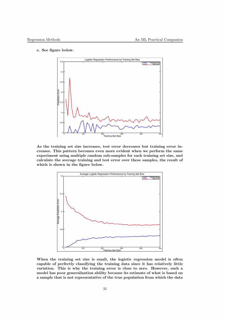
e. See figure below.
As the training set size increases, test error decreases but training error in-creases. This pattern becomes even more evident when we perform the sameexperiment using multiple random sub-samples for each training set size, andcalculate the average training and test error over these samples, the result ofwhich is shown in the figure below.
When the training set size is small, the logistic regression model is oftencapable of perfectly classifying the training data since it has relatively littlevariation. This is why the training error is close to zero. However, such amodel has poor generalization ability because its estimate of what is based ona sample that is not representative of the true population from which the data
31

An ML Practical Companion Regression Methods
is drawn. This phenomenon is known as overfitting because the model fits tooclosely to the training data. As the training set size increases, more variationis introduced into the training data, and the model is usually no longer ableto fit to the training set as well. This is also due to the fact that the completedataset is not 100% linearly separable. At the same time, more training dataprovides the model with a more complete picture of the overall population,which allows it to learn a more accurate estimate of wHat. This in turn leadsto better generalization ability i.e. lower prediction error on the test dataset.
f. The analytical formula for the decision boundary is given by w0+∑P
j=1 wjxj =0. This is the equation for a hyperplane in R
p, which indicates that the decisionboundary is linear.
g. See the function PlotDB in the solution code. See the figure below.
32
Regression Methods An ML Practical Companion
13. (Logistic Regression (with gradient ascent)xxx and Rosenblatt’s Perceptron:xxx application on the Breast Cancer datasetxxx n-fold cross-validation; confidence interval)
• (CMU, 2009 spring, Ziv Bar-Joseph, HW2, pr. 4)
For this exercise, you will use the Breast Cancer dataset, downloadable fromthe course web page. Given 9 different attributes, such as “uniformity of cellsize”, the task is to predict malignancy.891 The archive from the course webpage contains a Matlab method loaddata.m, so you can easily load in the databy typing (from the directory containing loaddata.m): data = loaddata. Thevariables in the resulting data structure relevant for you are:
• data.X: 683 9-dimensional data points, each element in the interval [1, 10].• data.Y: the 683 corresponding classes, either 0 (benign), or 1 (malignant).
Logistic Regression
a. Write code in Matlab to train the weights for logistic regression. To avoiddealing with the intercept term explicitly, you can add a nonzero-constanttenth dimension to data.X: data.X(:,10)=1. Your regression function thus be-comes simply:
P (Y = 0|x;w) =1
1 + exp(∑10
k=1 xkwk)
P (Y = 1|x;w) =exp(
∑10k=1 xkwk)
1 + exp(∑10
k=1 xkwk)
and the gradient-ascend update rule:
w← w + α/683
683∑
j=1
xj(yj − P (Y j = 1|xj ;w))
Use the learning rate α = 1/10. Try different learning rates if you cannot getw to converge.
b. To test your program, use 10-fold cross-validation, splitting [data.X data.Y]into 10 random approximately equal-sized portions, training on 9 concatenatedparts, and testing on the remaining part. Report the mean classificationaccuracy over the 10 runs, and the 95% confidence interval.
Rosenblatt’s Perceptron
A very simple and popular linear classifier is the perceptron algorithm ofRosenblatt (1962), a single-layer neural network model of the form
y(x) = f(w⊤x),
with the activation function
f(a) =
1 if a ≥ 0−1 otherwise.
891For more information on what the individual attributes mean, see ftp://ftp.ics.uci.edu/pub/machine-learning-databases/breast-cancer-wisconsin/breastcancer-wisconsin.names.
33
An ML Practical Companion Regression Methods
For this classifier, we need our classes to be −1 (benign) and 1 (malignant),which can be achieved with the Matlab command: data.Y = data.Y ⋆ 2 - 1.
Weight training usually proceeds in an online fashion, iterating through theindividual data points xj one or more times. For each xj, we compute thepredicted class yj = f(w⊤xj) for xj under the current parameters w, and updatethe weight vector as follows:
w ← w + xj [yj − yj ].
Note how w only changes if xj was misclassified under the current model.
c. Implement this training algorithm in Matlab. To avoid dealing with the in-tercept term explicitly, augment each point in data.X with a non-zero constanttenth element. In Matlab this can be done by typing: data.X(:,10)=1. Haveyour algorithm iterate through the whole training data 20 times and report thenumber of examples that were still mis-classified in the 20th iteration. Doesit look like the training data is linearly separable? (Hint: The perceptronalgorithm is guaranteed to converge if the data is linearly separable.)
d. To test your program, use 10-fold cross-validation, using the splits youobtained in part b. For each split, do 20 training iterations to train the wei-ghts. Report the mean classification accuracy over the 10 runs, and the 95%confidence interval.
e. If the data is not linearly separable, weights can toggle back and forthfrom iteration to iteration. Even in the linearly separable case, the learnedmodel is often very dependent on which training data points come first in thetraining sequence. A simple improvement is the weighted perceptron : trainingproceeds as before, but the weight vector w is saved after each update. Aftertraining, instead of the final w, the average of all saved w is taken to bethe learned weight vector. Report 10-fold CV accuracy for this variant andcompare it to the simple perceptron’s.
Solution:
You should have gotten something like this:
b. mean accuracy: 0.965, confidence interval: (0.951217, 0.978783).
c. 30 mis-classifications in the 20th iteration. (Note that using the trainedweights *after* the 20th iteration results in only around 24 mis-classifications.)When running with 200 iterations, still more than 20 mis-classifications occur,so the data is unlikely to be linearly separable as otherwise the training errorwould become zero after many enough iterations.
d. Perceptron:mean accuracy = 0.956, 95% confidence interval: (0.940618, 0.971382).
e. Weighted perceptron:mean accuracy = 0.968, 95% confidence interval: (0.954800, 0.981200).
34

Regression Methods An ML Practical Companion
14. (Logistic regression with gradient ascent:xxx application to text classification)
• CMU, 2010 fall, Aarti Singh, HW1, pr. 5
In this problem you will implement Logistic Regression and evaluate its per-formance on a document classification task. The data for this task is takenfrom the 20 Newsgroups data set,892 and is available from the course webpage.
Our model will use the bag-of-words assumption. This model assumes thateach word in a document is drawn independently from a categorical distribu-tion over possible words. (A categorical distribution is a generalization of aBernoulli distribution to multiple values.) Although this model ignores theordering of words in a document, it works surprisingly well for a number oftasks. We number the words in our vocabulary from 1 to m, where m is thetotal number of distinct words in all of the documents. Documents from classy are drawn from a class-specific categorical distribution parameterized by θy.θy is a vector, where θy,i is the probability of drawing word i and
∑mi=1 θy,i = 1.
Therefore, the class-conditional probability of drawing document x from ourmodel is
P (X = x|Y = y) =m∏
i=1
θcounti(x)y,i ,
where counti(x) is the number of times word i appears in x.
a. Provide high-level descriptions of the Logistic Regression algorithm. Besure to describe how to estimate the model parameters and how to classify anew example.
b. Implement Logistic Regression. We found that a step size around 0.0001worked well. Train the model on the provided training data and predict thelabels of the test data. Report the training and test error.
Solution:
a. The logistic regression model is
P (Y = 1|X = x,w) =exp(w0 +
∑
i wixi)
1 + exp(w0 +∑
iwixi),
where w = (w0, w1, . . . , wm)⊤ is our parameter vector. We will find w by maxi-mizing the data loglikelihood l(w):
l(w) = log
∏
j
exp(yj(w0 +∑
iwixji ))
1 + exp(w0 +∑
i wixji )
=∑
j
(
yj(w0 +∑
i
wixji )− log(1 + exp(w0 +
∑
i
wixji ))
)
We can estimate/learn the parameters (w) of logistic regression by optimi-zing l(w), using gradient ascent. The gradient of l(w) is the array of partialderivatives of l(w):
892Full version available from http://people.csail.mit.edu/jrennie/20Newsgroups/.
35

An ML Practical Companion Regression Methods
∂l(w)
∂w0=
∑
j
(
yj − exp(w0 +∑
i wixji )
1 + exp(w0 +∑
iwixji )
)
=∑
j
(yj − P (Y = 1|X = xj ;w))
∂l(w)
∂wk=
∑
j
(
yjxjk −
xjk exp(w0 +
∑
i wixji )
1 + exp(w0 +∑
iwixji )
)
=∑
j
xjk(y
j − P (Y = 1|X = xj ;w))
Let w(t) represent our parameter vector on the t-th iteration of gradient ascent.To perform gradient ascent, we first set w(0) to some arbitrary value (say 0).We then repeat the following updates until convergence:
w(t+1)0 ← w
(t)0 + α
∑
j
(
yj − P (Y = 1|X = xj ;w(t)))
w(t+1)k ← w
(t)k + α
∑
j
xjk
(
yj − P (Y = 1|X = xj ;w(t)))
where α is a step size parameter which controls how far we move along ourgradient at each step. We set α = 0.0001. The algorithm converges when||w(t)−w(t+1)|| < δ, that is when the weight vector doesn’t change much duringan iteration. We set δ = 0.001.
b. Training error: 0.00. Test error: 0.29. The large difference between trainingand test error means that our model overfits our training data. A possiblereason is that we do not have enough training data to estimate either modelaccurately.
36

Regression Methods An ML Practical Companion
15. (Logistic regression, regularized (L2):xxx application to binary text classification;xxx feature selection using mutual information)
• CMU, 2012 fall, T. Mitchell, Z. Bar-Joseph, HW2, pr. 4
37
An ML Practical Companion Regression Methods
16. (Logistic regression using Newton’s method:xxx application on R
2 data)
• Stanford, 2011 fall, Andrew Ng, HW1, pr. 1.bc
a. On the web page associated to this booklet, you will find the files q1x.dat
and q1y.dat which contain the inputs (x(i) ∈ R2) and outputs (y(i) ∈ 0, 1) res-
pectively for a binary classification problem, with one training example perrow.
Implement Newton’s method for optimizing ℓ(θ), the [conditional] log-likelihoodfunction
ℓ(θ) =
m∑
i=1
y(i) lnσ(w · x(i)) + (1− y(i)) ln(1 − σ(w · x(i))),
and apply it to fit a logistic regression model to the data. Initialize Newton’smethod with θ = 0 (the vector of all zeros). What are the coefficients θresulting from your fit? (Remember to include the intercept term.)
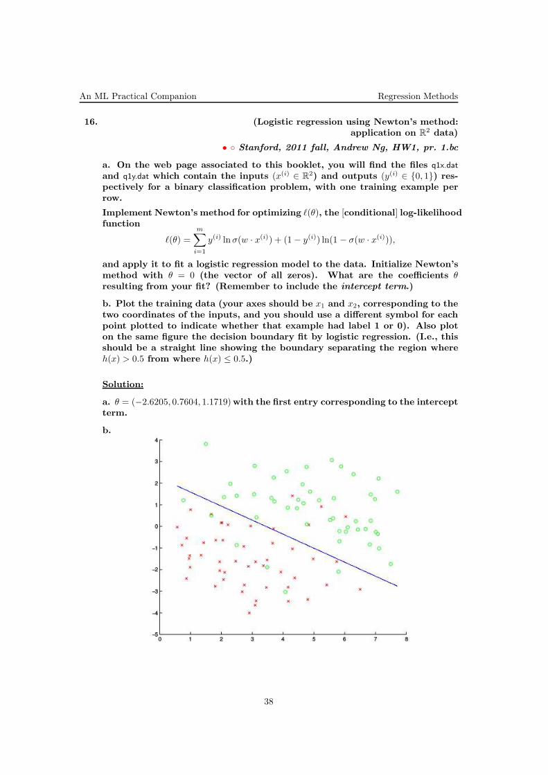
b. Plot the training data (your axes should be x1 and x2, corresponding to thetwo coordinates of the inputs, and you should use a different symbol for eachpoint plotted to indicate whether that example had label 1 or 0). Also ploton the same figure the decision boundary fit by logistic regression. (I.e., thisshould be a straight line showing the boundary separating the region whereh(x) > 0.5 from where h(x) ≤ 0.5.)
Solution:
a. θ = (−2.6205, 0.7604, 1.1719)with the first entry corresponding to the interceptterm.
b.
38
Regression Methods An ML Practical Companion
17. (Solving logistic regression, the kernelized version,xxx using the gradient method:xxx implementation + application on R
2 data)
• CMU, 2005 fall, Tom Mitchell, HW3, pr. 2.cd
a. Implement the kernel logistic regression described in ex. ?? in our exercise
book, using the gaussian kernel Kτ (x, x′) = exp
(‖x− x′‖22τ2
)
.
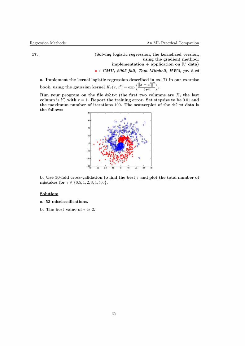
Run your program on the file ds2.txt (the first two columns are X, the lastcolumn is Y ) with τ = 1. Report the training error. Set stepsize to be 0.01 andthe maximum number of iterations 100. The scatterplot of the ds2.txt data isthe follows:
b. Use 10-fold cross-validation to find the best τ and plot the total number ofmistakes for τ ∈ 0.5, 1, 2, 3, 4, 5, 6.
Solution:
a. 53 misclassifications.
b. The best value of τ is 2.
39
An ML Practical Companion Regression Methods
18. (Locally-weighted, regularized (L2) logistic regression,xxx using Newton’s method:xxx application on dataset from R
2)
• Stanford, 2007 fall, Andrew Ng, HW1, pr. 2
In this problem you will implement a locally-weighted version of logistic re-gression which was described in the ?? exercise in the Estimating the parame-ters of some probabilistic distributions chapter of our exercise book. For theentirety of this problem you can use the value λ = 0.0001.
Given a query point x, we choose compute the weights
wi = exp
(
−‖x− xi‖22τ2
)
.
This scheme gives more weight to the “nearby” points when predicting theclass of a new example[, much like the locally weighted linear regression dis-cussed at exercise ??].
a. Implement the Newton algorithm for optimizing the log-likelihood function(ℓ(θ) in the ?? exercise) for a new query point x, and use this to predict theclass of x. The q2/ directory contains data and code for this problem. Youshould implement the y = lwlr(X_train, y_train, x, tau) function in the lwlr.mfile. This function takes as input the training set (the X_train and y_trainmatrices), a new query point x and the weight bandwitdh tau. Given thisinput, the function should i . compute weights wi for each training example,using the formula above, ii . maximize ℓ(θ) using Newton’s method, and iii .output y = 1hθ(x)>0.5 as the prediction.
We provide two additional functions that might help. The [X_train, y_train] =load_data; function will load the matrices from files in the data/ folder. Thefunction plot_lwlr(X_train, y_train, tau, resolution) will plot the resulting classifier(assuming you have properly implemented lwlr.m). This function evaluates thelocally weighted logistic regression classifier over a large grid of points andplots the resulting prediction as blue (predicting y = 0) or red (predictingy = 1). Depending on how fast your lwlr function is, creating the plot mighttake some time, so we recommend debugging your code with resolution = 50; andlater increase it to at least 200 to get a better idea of the decision boundary.
b. Evaluate the system with a variety of different bandwidth parameters τ .In particular, try τ = 0.01, 0.05, 0.1, 0.5, 1.0, 5.0. How does the classificationboundary change when varying this parameter? Can you predict what thedecision boundary of ordinary (unweighted) logistic regression would looklike?
Solution:
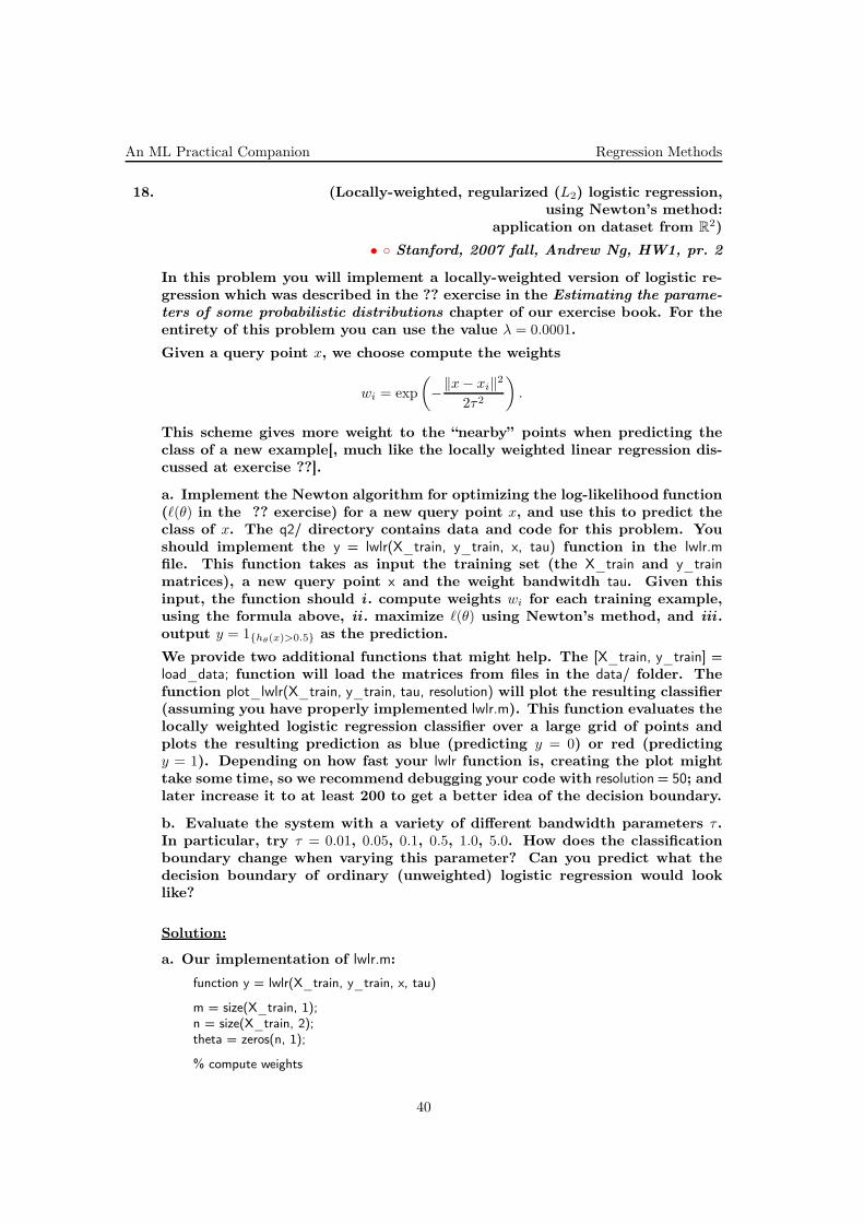
a. Our implementation of lwlr.m:
function y = lwlr(X_train, y_train, x, tau)
m = size(X_train, 1);n = size(X_train, 2);theta = zeros(n, 1);
% compute weights
40
Regression Methods An ML Practical Companion
w = exp(-sum((X_train - repmat(x’, m, 1)).∧2, 2) / (2*tau));
% perform Newton’s methodg = ones(n, 1);while (norm(g) > 1e-6)
h = 1 ./ (1 + exp(-X_train * theta));g = X_train’ * (w.*(y_train - h)) - 1e-4*theta;H = -X_train’ * diag(w.*h.*(1-h)) * X_train - 1e-4*eye(n);theta = theta - H g;
end
% return predicted yy = double(x’*theta > 0);
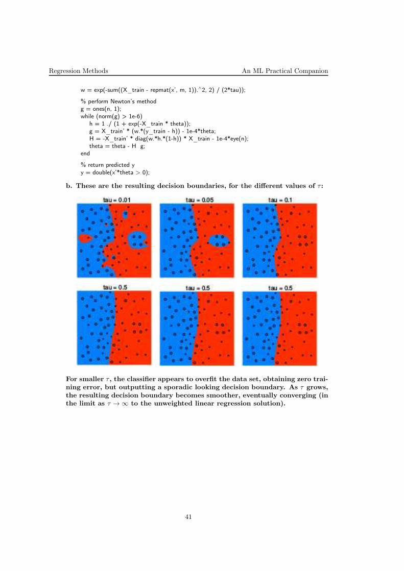
b. These are the resulting decision boundaries, for the different values of τ :
For smaller τ , the classifier appears to overfit the data set, obtaining zero trai-ning error, but outputting a sporadic looking decision boundary. As τ grows,the resulting decision boundary becomes smoother, eventually converging (inthe limit as τ →∞ to the unweighted linear regression solution).
41
An ML Practical Companion Regression Methods
19. (Logistic regression with L2 regularization;xxx application on handwritten digit recognition;xxx comparison between the stochastic gradient method and Newton’smethod)
• MIT, 2001 fall, Tommi Jaakkola, HW2, pr. 4
Here you will solve a digit classification problem with logistic regression mo-dels. We have made available the following training and test sets: digit_x.dat,digit_y.dat, digit_x_test.dat, digit_y_test.dat.
a. Derive the stochastic gradient ascent learning rule for a logistic regressionmodel starting from the regularized likelihood objective
J(w; c) = . . .
where ‖w‖2 =∑d
i=0 w2i [or by modifying your derivation of the delta rule for
the softmax model]. (Normally we would not include w0 in the regularizationpenalty but have done so here for simplicity of the resulting update rule).
b. Write a MATLAB function w = SGlogisticreg(X,y,c,epsilon) that takes inputs si-milar to logisticreg from the previous section, and a learning rate parameterε, and uses stochastic gradient ascent to learn the weights. You may includeadditional parameters to control when to stop, or hard-code it into the func-tion.
c. Provide a rationale for setting the learning rate and the stopping criterionin the context of the digit classification task. You should assume that theregularization parameter c remains fixed at 1. (You might wish to experimentwith different learning rates and stopping criterion but do NOT use the testset. Your justification should be based on the available information beforeseeing the test set.)
d. Set c = 1 and apply your procedure for setting the learning rate and thestopping criterion to evaluate the average log-probability of labels in the trai-ning and test sets. Compare the results to those obtained with logisticreg. Foreach optimization method, report the average log-probabilities for the labelsin the training and test sets as well as the corresponding mean classificationerrors (estimates of the miss-classification probabilities). (Please include allMATLAB code you used for these calculations.)
e. Are the train/test differences between the optimization methods reasona-ble? Why? (Repeat the gradient ascent procedure a couple of times to ensurethat you are indeed looking at a “typical” outcome.)
f. The classifiers we found above are both linear classifiers, as are all logisticregression classifiers. In fact, if we set c to a different value, we are stillsearching the same set of linear classifiers. Try using logisticreg with differentvalues of c, to see that you get different classifications. Why are the resultingclassifiers different, even though the same set of classifiers is being searched?Contrast the reason with the reason for the differences you explained in theprevious question.
g. Gaussian mixture models with identical covariance matrices also lead tolinear classifiers. Is there a value of c such that training a Gaussian mix-ture model necessarily leads to the same classification as training a logisticregression model using this value of c? Why?
42

Regression Methods An ML Practical Companion
Solution:
a.w←
(
1− ε c
n
)
w + ε(yi − P (1|xi, w))xi.
[LC: You can find the details in the MIT document.]
b.
function [w] = SGlogisticreg(X,y,c,epsilon,stopdelta)[n,d] = size(X);X = [ones(n,1),X];w = zeros(d+1,1);cont = 1;while (cont)
perm = randperm(n);oldw = w;for i = 1:n
w = (1 - epsilon * c / n) * w + epsilon * (y(i) - g(X(i,:) * w)) * X(i,:)’ ;endcont = norm(oldw - w) >= stopdelta * norm(oldw) ;
end
c. Learning rate: If the learning rate is too high, any memory of previousupdates will be wiped out (beyond the last few points used in the updates).It’s important that all the points affect the resulting weights and so the lear-ning rate should scale somehow with the number of examples. But how?When the stochastic gradient updates converge, we are not changing the wei-ghts on average. So each update can be seen as a slight random perturbationaround the correct weights. We’d like to keep such stochastic effects frompushing the weights too far from the optimal solution. One way to deal withthis is to simply average the random effects by making the learning rate scale
as ε =c
nfor a constant c, somewhat less than one.
But this would be slow. It’s good to keep the variance of the sum of the
random perturbation at a constant and instead set ε =c√n: You may recall
that if Zi is a Gaussian with zero zero and unit variance, then∑
i = 1nZi
has variance n. Here Zi corresponds to a gradient update based on the i-th example. Dividing by the standard deviation of the sum,
√n, makes the
gradient updates have an overall fixed variance.
Since the update is also proportional to the norm of the input examples youmight also divide the learning rate by the overall scale of the inputs. If wehave d binary coordinates, the norm is at most d. We get a learning rate of
ε =c√n d
.
Stopping criterion : We want to stop when a full iteration through the trainingset does not make much difference on average. Note that unless we canperfectly separate the training set, we would still expect to get specific trainingexamples that will cause change, but at convergence they should cancel eachother out. We should also not stop just because one, or a few, examples didnot cause much change -– it might be that other examples will.
And so, after each full iteration through the training set, we see how muchthe weight changed since before the iteration. As we do not know what the
43
An ML Practical Companion Regression Methods
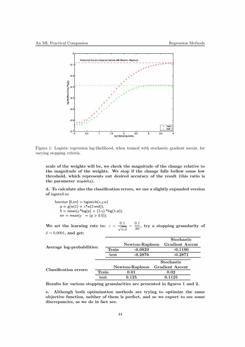
Figura 1: Logistic regression log-likelihood, when trained with stochastic gradient ascent, forvarying stopping criteria.
scale of the weights will be, we check the magnitude of the change relative tothe magnitude of the weights. We stop if the change falls bellow some lowthreshold, which represents out desired accuracy of the result (this ratio isthe parameter stopdelta).
d. To calculate also the classification errors, we use a slightly expanded versionof logisticll.m:
function [ll,err] = logisticle(x,y,w)p = g(w(1) + x*w(2:end));ll = mean(y.*log(p) + (1-y).*log(1-p));err = mean(y ˜ = (p > 0.5));
We set the learning rate to: ε =0.1√n d
=0.1
80, try a stopping granularity of
δ = 0.0001, and get:
Average log-probabilities:
StochasticNewton-Raphson Gradient Ascent
Train -0.0829 -0.1190test -0.2876 -0.2871
Classification errors:
StochasticNewton-Raphson Gradient Ascent
Train 0.01 0.02test 0.125 0.1125
Results for various stopping granularities are presented in figures 1 and 2.
e. Although both optimization methods are trying to optimize the sameobjective function, neither of them is perfect, and so we expect to see somediscrepancies, as we do in fact see.
44
Regression Methods An ML Practical Companion
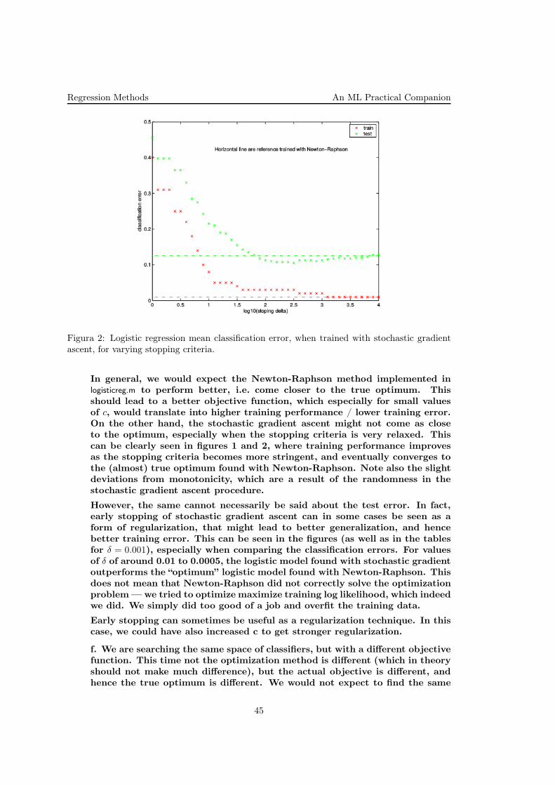
Figura 2: Logistic regression mean classification error, when trained with stochastic gradientascent, for varying stopping criteria.
In general, we would expect the Newton-Raphson method implemented inlogisticreg.m to perform better, i.e. come closer to the true optimum. Thisshould lead to a better objective function, which especially for small valuesof c, would translate into higher training performance / lower training error.On the other hand, the stochastic gradient ascent might not come as closeto the optimum, especially when the stopping criteria is very relaxed. Thiscan be clearly seen in figures 1 and 2, where training performance improvesas the stopping criteria becomes more stringent, and eventually converges tothe (almost) true optimum found with Newton-Raphson. Note also the slightdeviations from monotonicity, which are a result of the randomness in thestochastic gradient ascent procedure.
However, the same cannot necessarily be said about the test error. In fact,early stopping of stochastic gradient ascent can in some cases be seen as aform of regularization, that might lead to better generalization, and hencebetter training error. This can be seen in the figures (as well as in the tablesfor δ = 0.001), especially when comparing the classification errors. For valuesof δ of around 0.01 to 0.0005, the logistic model found with stochastic gradientoutperforms the “optimum” logistic model found with Newton-Raphson. Thisdoes not mean that Newton-Raphson did not correctly solve the optimizationproblem — we tried to optimize maximize training log likelihood, which indeedwe did. We simply did too good of a job and overfit the training data.
Early stopping can sometimes be useful as a regularization technique. In thiscase, we could have also increased c to get stronger regularization.
f. We are searching the same space of classifiers, but with a different objectivefunction. This time not the optimization method is different (which in theoryshould not make much difference), but the actual objective is different, andhence the true optimum is different. We would not expect to find the same
45

An ML Practical Companion Regression Methods
classifier.
g. There is no such value of c. The objective functions are different, evenfor c = 0. The logistic regression objective function aims to maximize thelikelihood of the labels given the input vectors, while the Gaussian mixtureobjective is to fit a probabilistic model for the training input vectors andlabels, by maximizing their joint joint likelihood.
46

Regression Methods An ML Practical Companion
20. (Multi-class regularized (L2) Logistic Regressionxxx with gradient ascent:xxx application to hand-written digit recognition)
• CMU, 2014 fall, W. Cohen, Z. Bar-Joseph, HW3, pr. 1xxx CMU, 2011 spring, Tom Mitchell, HW3, pr. 2
A. In this part of the exercise you will implement the two class Logistic Re-gression classifier and evaluate its performance on digit recognition.
The dataset we are using for thisassignment is a subset of theMNIST handwritten digit data-base,893 which is a set of 70,000 28× 28 handwritten digits from a mi-xture of high school students andgovernment Census Bureau em-ployees.
Your goal will be to write a logis-tic regression classifier to distingu-ish between a collection of 4s and 7s,of which you can see some examplesin the nearby figure.
The data is given to you in the formof a design matrix X and a vec-tor y of labels indicating the class.There are two design matrices, onefor training and one for evaluation.The design matrix is of size m × n, where m is the number of examples andn is the number of features. We will treat each pixel as a feature, giving usn = 28× 28 = 784.
Given a set of training points x1, x2, . . . , xm and a set of labels y1, . . . , ym we wantto estimate the parameters of the model w. We can do this by maximizingthe log-likelihood function.894
Given the sigmoid / logistic function,
σ(x) =1
1 + e−x,
the cost function and its gradient are
J(w) =λ
2||w||22 −
m∑
i=1
yi log σ(w⊤xi) + (1− yi) log(1− σ(w⊤xi))
∇J(w) = λw −m∑
i=1
(yi − σ(w⊤xi))xi
Note (1): The cost function contains the regularization term,λ
2||w||22. Regu-
larization forces the parameters of the model to be pushed towards zero by
893Y. LeCun, L. Bottou, Y. Bengio, and P. Haffner, Gradient-based learning applied to document recognition.Proceedings of the IEEE 86, 11 (Nov 1998), pp. 2278–2324.894LC: For the derivation of the update rule for logistic regression (together with an L2 regularization term),
see CMU, 2012 fall, T. Mitchell, Z. Bar-Joseph, HW2, pr. 2.
47
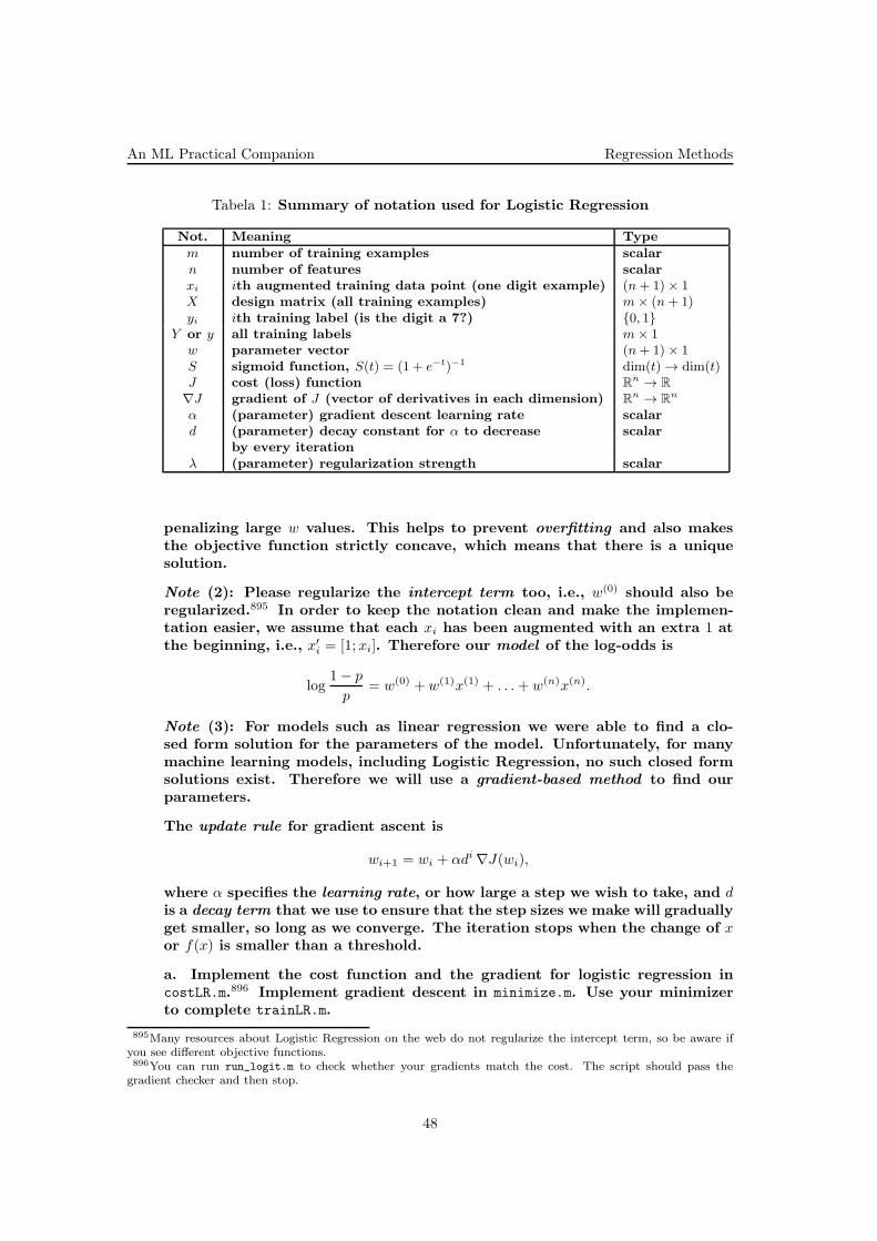
An ML Practical Companion Regression Methods
Tabela 1: Summary of notation used for Logistic Regression
Not. Meaning Typem number of training examples scalarn number of features scalarxi ith augmented training data point (one digit example) (n+ 1)× 1X design matrix (all training examples) m× (n+ 1)yi ith training label (is the digit a 7?) 0, 1
Y or y all training labels m× 1w parameter vector (n+ 1)× 1S sigmoid function, S(t) = (1 + e−t)−1 dim(t) → dim(t)J cost (loss) function R
n → R
∇J gradient of J (vector of derivatives in each dimension) Rn → R
n
α (parameter) gradient descent learning rate scalard (parameter) decay constant for α to decrease scalar
by every iterationλ (parameter) regularization strength scalar
penalizing large w values. This helps to prevent overfitting and also makesthe objective function strictly concave, which means that there is a uniquesolution.
Note (2): Please regularize the intercept term too, i.e., w(0) should also beregularized.895 In order to keep the notation clean and make the implemen-tation easier, we assume that each xi has been augmented with an extra 1 atthe beginning, i.e., x′
i = [1;xi]. Therefore our model of the log-odds is
log1− p
p= w(0) + w(1)x(1) + . . .+ w(n)x(n).
Note (3): For models such as linear regression we were able to find a clo-sed form solution for the parameters of the model. Unfortunately, for manymachine learning models, including Logistic Regression, no such closed formsolutions exist. Therefore we will use a gradient-based method to find ourparameters.
The update rule for gradient ascent is
wi+1 = wi + αdi∇J(wi),
where α specifies the learning rate, or how large a step we wish to take, and dis a decay term that we use to ensure that the step sizes we make will graduallyget smaller, so long as we converge. The iteration stops when the change of xor f(x) is smaller than a threshold.
a. Implement the cost function and the gradient for logistic regression incostLR.m.896 Implement gradient descent in minimize.m. Use your minimizerto complete trainLR.m.
895Many resources about Logistic Regression on the web do not regularize the intercept term, so be aware ifyou see different objective functions.896You can run run_logit.m to check whether your gradients match the cost. The script should pass the
gradient checker and then stop.
48
Regression Methods An ML Practical Companion
b. Once you have trained the model, you can then use it to make predictions.Implement predictLR, which will generate the most likely classes for a givenxi.
B. In this part of the exercise you will implement the multi-class class LogisticRegression classifier and evaluate its performance on another digit recognition,provided by USPS. In this dataset, each hand-written digital image is 16 by16 pixels. If we treat the value of each pixel as a boolean feature (either 0for black or 1 for white), then each example has 16 × 16 = 256 0, 1-valuedfeatures, and hence x has 256 dimension. Each digit (i.e., 1,2,3,4,5,6,7,8,9,0)corresponds to a class label y (y = 1, . . . ,K, K = 10). For each digit, we have600 training samples and 500 testing samples.897
Please download the data from the website. Load the usps digital.mat file inusps_digital.zip into Matlab. You will have four matrices:
• tr_X: training input matrix with the dimension 6000× 256.
• tr_y: training label of the length 6000, each element is from 1 to 10.
• te_X: testing input matrix with the dimension 5000× 256.
• te_y: testing label of the length 5000, each element is from 1 to 10.
For those who do NOT want to use Matlab, we also provide the text filefor these four matrices in usps_digital.zip. Note that if you want to viewthe image of a particular training/testing example in Matlab, say the 1000thtraining example, you may use the following Matlab command:imshow(reshape(tr_X(1000,:),16,16)).
c. Use the gradient ascent algorithm to train a multi-class logistic regressionclassifier. Plot (1) the objective value (log-likelihood), (2) the training accu-racy, and (3) the testing accuracy versus the number of iterations. Reportyour final testing accuracy, i.e., the fraction of test images that are correctlyclassified.
Note that you must choose a suitable learning rate (i.e. stepsize) of thegradient ascent algorithm. A hint is that your learning rate cannot be toolarge otherwise your objective will increase only for the first few iterations.
In addition, you need to choose a suitable stopping criterion. You might usethe number of iterations, the decrease of the objective value, or the maxi-mum of the L2 norms of the gradient with respect to each wk. Or you mightwatch the increase of the testing accuracy and stop the optimization when theaccuracy is stable.
d. Now we add the regularization termλ
2
∑K−1i=1 ||wl||22. For λ = 1, 10, 100, 1000,
report the final testing accuracies.
e. What can you conclude from the above experiment? (Hint: the relationshipbetween the regularization weight and the prediction performance.)
Solution:
b. You should get about 96% accuracy.
897You can view these images at http://www.cs.nyu.edu/∼roweis/data/usps_0.jpg, . . . ,http://www.cs.nyu.edu/∼roweis/data/usps_9.jpg.
49

An ML Practical Companion Regression Methods
c. I use the stepsize η = 0.0001 and run the gradient ascent method for 5000iterations. The objective value vs. the number of iterations, training errorvs. the number of iterations, testing error vs. the number of iterations arepresented in figure below:
d. For λ = 0, 1, 10, 100, 1000, the comparison of the testing accuracy is presentedin the next table:
λ 0 1 10 100 1000Testing accuracy 91.44% 91.58% 91.92% 89.74% 79.78%
e. From the above result, we can see that adding the regularization couldavoid overfitting and lead to better generalization performance (e.g., λ = 1, 10).However, the regularization cannot be too large. Although a larger regulari-zation can decrease the variance, it introduces additional bias and may leadto worse generalization performance.
50

Regression Methods An ML Practical Companion
21. (Multinomial/Categorical Logistic Regression,xxx Gaussian Naive Bayes, Gaussian Joint Bayes, and k-NN:xxx application on the ORL Faces dataset)
• · CMU 2010 spring, E. Xing, T. Mitchell, A. Singh, HW2, pr. 2
In this part, you are going to play with The ORL Database of Faces.
6 sample images from two persons
Each image is 92 by 112 pixels. If we treat the luminance of each pixel asa feature, each sample has 92 ∗ 112 = 10304 real value features, which canbe written as a random vector X. We will treat each person as a class Y(Y = 1, . . . ,K, K = 10). We use Xi to refer the i-th feature. Given a setof training data D = (yl, xl), we will train different classification models toclassify images to their person id’s. To simplify notation, we will use P (y|x)in place of P (Y = y|X = x).
We will select our models by 10-fold cross validation: partition the data foreach face into 10 mutually exclusive sets (folds). In our case, exactly oneimage for each fold. Then, for k = 1, . . . , 10, leave out the data from fold k forall faces, train on the rest, and test on the left out data. Average the resultsof these 10 tests to estimate the training accuracy of your classifier.
Note: Beware that we are actually not evaluating the generalization errors ofthe classifier here. When evaluating generalization error, we would need anindependent test set that is not at all touched during the whole developingand tuning process.
For your convenience, a piece of code loadFaces.m is provided to help loadingimages as feature vectors.
From Tom Mitchell’s additional book chapter,898 page 13, you will see a gene-ralization of logistic regression, which allows Y to have more than two possiblevalues.
a. Write down the objective function, and the first order derivatives of themultinomial logistic regression model (which is a binary classifier).899
Here we will consider a L2-norm regularized objective function (with a termλ|θ|2).
b. Implement the logistic regression model with gradient ascent. Show yourevaluation result here. Use regularization parameter λ = 0.
898www.cs.cmu.edu/∼tom/mlbook/NBayesLogReg.pdf.899Hint : In order to do k-class classification with binary classifier, we use a voting scheme. At training time,
a classifier is trained for any pair of classes. At testing time, all k(k − 1)/2 classifiers are applied to the testingsample. Each classifier either vote for its first class or its second class. The class voted by most number ofclassifiers is chosen as the prediction.
51

An ML Practical Companion Regression Methods
Hint : The gradient ascent method (also known as steepest ascent) is a first-order optimization algorithm. It optimizes a function f(x) by
xt+1 = xt + αtf′(xt),
where αt is called the step size, which is often picked by line search. Forexample, we can initialize αt = 1.0. Then set αt = αt/2 while f(xt + αtf
′(xt)) <f(xt). The iteration stops when the change of x or f(x) is smaller than athreshold.
Hint : If the training time of your model is too long, you can consider use justa subset of the features (e.g., in Matlab X = X(:,1:100:d)).
c. Overfitting and Regularization
Now we test how regularization can help prevent overfitting. During cross-validation, let’s use m images from each person for training, and the restfor testing. Report your cross-validated result with varying m = 1, . . . , 9 andvarying regularization parameter λ.
d. Logistic Regression and Newton’s method
Newton’s method (also known as the Newton-Raphson method) is a first-order optimization algorithm, which often converges in a few iterations. ItOptimize a function f(x) by the update equation
xt+1 = xt −f ′(xt)
f ′′(xt)
The iteration stops when the change of x or f(x) is smaller than a threshold.Write down the second order derivatives and the update equation of the lo-gistic regression model.
Implement the logistic regression model with Newton’s method. Show yourevaluation result here.
B. Implement the k-NN algorithm. Use L2-norm as the distance metric. Showyour evaluation result here, and compare different values of k.
C. Conditional Gaussian Estimation
For a Gaussian model we have
P (y|x) = P (x|y)P (y)
P (x),
where
P (x|y) = 1
(2π)d/2|Σy|1/2exp(−(x− µy)
⊤Σ−1(x− µy)/2),
and P (y) = πy. Please write down the MLE estimation of model parametersΣy, µy, and πy. Here we do not assume that Xi are independent given Y .
D. Gaussian Naive Bayes is a form of Guassian model with assumption thatXi are independent given Y . Implement the Gaussian NB model, and brieflydescribe your evaluation result.
E. Compare the above methods by training/testing time, and accuracy.Which method do you prefer?
52

Regression Methods An ML Practical Companion
22. (Model selection:xxx sentiment analysis for music reviewsxxx using a dataset provided by Amazon,xxx using lasso logistic regression)
• · CMU, 2014 spring, B. Poczos, A. Singh, HW2, pr. 5
In this homework, you will perform model selection on a sentiment analysisdataset of music reviews.900 The dataset consists of reviews from Amazon.comfor musics. The ratings have been converted to a binary label, indicating anegative review or a positive review. We will use lasso logistic regression forthis problem.901 The lasso logistic regression objective function to minimizeduring training is:
L(β) = log(1 + exp(−yβ⊤x)) + λ‖β‖1
In lasso logistic regression, we penalize the loss function by an L1 norm ofthe feature coefficients. Penalization with an L1 norm tends to produce so-lutions where some coefficients are exactly 0. This makes it attractive forhigh-dimensional data such as text, because in most cases most words cantypically be ignored. Furthermore, since we are often left with only a fewnonzero coefficients, the lasso solution is often easy to interpret.
The goal of model selection here is to choose λ since each setting of λ impliesa different model size (number of non-zero coefficients).
You do not need to implement lasso logistic regression. You can downloadan implementation from https://github.com/redpony/creg, and the dataset can befound on the course web page. There are three feature files and three response(label) files (all response files end with .res). They are already in the formatrequired by the implementation you will use. The files are:
• Training data: music.train and music.train.res
• Development data: music.dev and music.dev.res
• Test data: music.test and music.test.res
Important note: The code outputs accuracy , whereas you need to plot clas-sification error here. You can simply transform accuracy to error by using1− accuracy.
Error on development (validation) data
In the first part of the problem, we will use error on a development data tochoose λ. Run the model with λ = 10−8, 10−7, 10−6, . . . , 10−1, 1, 10, 100.a. Plot the error on training data and development data as a function of logλ.
b. Plot the model size (number of nonzero coefficients) on development dataas a function of logλ.
c. Choose λ that gives the lowest error on development data. Run it on thetest data and report the test error.
900John Blitzer, Mark Dredze, and Fernando Pereira. Biographies, Bollywood, Boom-boxes and Blenders:Domain Adaptation for Sentiment Classification. In Proceedings of ACL, 2007.901Robert Tibshirani. Regression shrinkage and selection via the lasso, In Journal of Royal Statistical Society
B, 58(1):267:288, 1996.
53

An ML Practical Companion Regression Methods
Briefly discuss all the results.
Model Complexity and Bias-Variance Tradeoff
d. Give a high-level explanation on the relation between λ and the bias andvariance of parameter estimates β. Does larger λ correspond to higher orlower bias? What about the variance? Does larger λ lead to a more complexor a less complex model?
Resolving a tie
e. If there are more than one λ that minimizes the error on the developmentdata, which one will you pick? Explain your choice.
Random search
f. An alternative way to search λ is by randomly sampling its value from aninterval.
i. Sample eleven random values log uniformly from an interval [10−8, 100] forλ and train a lasso logistic regression model. Plot the error on develop-ment data as a function of logλ.
ii. Choose λ that gives the lowest error on development data. Run it on thetest data and report the test error.
Random vs. grid search
g. Which one do you think is a better method for searching values to try forλ? Why?
54

Regression Methods An ML Practical Companion
23. (Metoda [sub-]gradientului:x diferite funcţii de cost / pierdere şix diferite funcţii / metode de regularizare)
• CMU, 2015 spring. Alex Smola, HW8, pr. 1
55
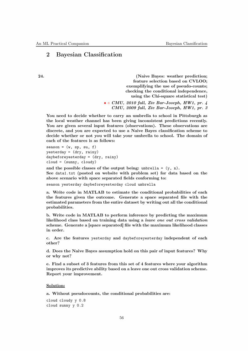
An ML Practical Companion Bayesian Classification
2 Bayesian Classification
24. (Naive Bayes: weather prediction;xxx feature selection based on CVLOO;xxx exemplifying the use of pseudo-counts;xxx checking the conditional independence,xxx using the Chi-square statistical test)
• CMU, 2010 fall, Ziv Bar-Joseph, HW1, pr. 4xxx CMU, 2009 fall, Ziv Bar-Joseph, HW1, pr. 3
You need to decide whether to carry an umbrella to school in Pittsburgh asthe local weather channel has been giving inconsistent predictions recently.You are given several input features (observations). These observations arediscrete, and you are expected to use a Naive Bayes classification scheme todecide whether or not you will take your umbrella to school. The domain ofeach of the features is as follows:
season = (w, sp, su, f)
yesterday = (dry, rainy)
daybeforeyesterday = (dry, rainy)
cloud = (sunny, cloudy)
and the possible classes of the output being: umbrella = (y, n).See data1.txt (posted on website with problem set) for data based on theabove scenario with space separated fields conforming to:
season yesterday daybeforeyesterday cloud umbrella
a. Write code in MATLAB to estimate the conditional probabilities of eachthe features given the outcome. Generate a space separated file with theestimated parameters from the entire dataset by writing out all the conditionalprobabilities.
b. Write code in MATLAB to perform inference by predicting the maximumlikelihood class based on training data using a leave one out cross validationscheme. Generate a [space separated] file with the maximum likelihood classesin order.
c. Are the features yesterday and daybeforeyesterday independent of eachother?
d. Does the Naive Bayes assumption hold on this pair of input features? Whyor why not?
e. Find a subset of 3 features from this set of 4 features where your algorithmimproves its predictive ability based on a leave one out cross validation scheme.Report your improvement.
Solution:
a. Without pseudocounts, the conditional probabilities are:
cloud cloudy y 0.8
cloud sunny y 0.2
56

Bayesian Classification An ML Practical Companion
cloud sunny n 0.6
cloud cloudy n 0.4
daybeforeyesterday dry y
daybeforeyesterday rainy
daybeforeyesterday dry n
daybeforeyesterday rainy
season w n 0.3
season sp n 0
season su n 0.3
season f n 0.4
season sp y 0.2
season su y 0.1
season f y 0.4
season w y 0.3
yesterday dry y 0.4
yesterday rainy y 0.6
yesterday rainy n 0.4
yesterday dry n 0.6
b. After adding pseudocounts, the ML classes for the data are:
yyynynnnnnnynnynyyynnynynnnnnyyynnnyynnn
Results may vary slightly because of the way pseudocounts are implemented.
c. Let yesterday be denoted by Y and daybeforeyesterday by D, and umbrella
by U.
Empirical Empirical Empirical ProductY D joint prob. prob. Y prob. D of the two
dry dry 0.3 0.5 0.5 0.25dry rain 0.2 0.5 0.5 0.25rain dry 0.2 0.5 0.5 0.25rain rain 0.3 0.5 0.5 0.25
Thus, they do not look independent from the data, but a stricter way to testis to subject it to a Chi-Square Test of independence. Since the number ofdata samples are low, we do not obtain a statistically significant result eitherway.
d. To check if the naive bayes assumption holds, we need to check for theconditional independence of the two given the umbrella label, so we partitionthe data based on the umbrella label and check for independence.
Empirical Empirical Empirical ProductU Y D joint prob. prob. Y prob. D of the twoy dry dry 0.2 0.4 0.4 0.16y dry rain 0.2 0.4 0.6 0.24y rain dry 0.2 0.6 0.4 0.24y rain rain 0.4 0.6 0.6 0.36n dry dry 0.4 0.6 0.6 0.36n dry rain 0.2 0.6 0.4 0.24n rain dry 0.2 0.4 0.6 0.24n rain rain 0.2 0.4 0.4 0.16
57

An ML Practical Companion Bayesian Classification
Again, they do not look independent, but the empirical joint probabilitiesand the product of the individual empirical probabilities look slightly closer.Again, a stricter way to test is to subject it to a Chi-Square Test of indepen-dence. Again, since the number of data samples are low, we do not obtain astatistically significant result either way.
e. Leaving out yesterday, using a LOOCV scheme, the percentage of correctlypredicted instances jumps from 55% to 75%.
58

Bayesian Classification An ML Practical Companion
25. (Naive Bayes: spam filtering)
• Stanford, 2012 spring, Andrew Ng, pr. 6xxx Stanford, 2015 fall, Andrew Ng, HW2, pr. 3.a-cxxx Stanford, 2009 fall, Andrew Ng, HW2, pr. 3.a-c
In this exercise, you will use Naive Bayes to classify email messages into spamand nonspam groups. Your dataset is a preprocessed subset of the Ling-SpamDataset,902 provided by Ion Androutsopoulos. It is based on 960 real emailmessages from a linguistics mailing list.
There are two ways to complete this exercise. The first option is to use theMatlab/Octave-formatted features we have generated for you. This requi-res using Matlab/Octave to read prepared data and then writing an imple-mentation of Naive Bayes. To choose this option, download the data packex6DataPrepared.zip.
The second option is to generate the features yourself from the emails and thenimplement Naive Bayes on top of those features. You may want this optionif you want more practice with features and a more open-ended exercise. Tochoose this option, download the data pack ex6DataEmails.zip.
Data Description:
The dataset you will be working with is split into two subsets: a 700-emailsubset for training and a 260-email subset for testing. Each of the trainingand testing subsets contain 50% spam messages and 50% nonspam messages.Additionally, the emails have been preprocessed in the following ways:1. Stop word removal: Certain words like “and,” “the,” and “of,” are verycommon in all English sentences and are not very meaningful in decidingspam/nonspam status, so these words have been removed from the emails.2. Lemmatization: Words that have the same meaning but different endingshave been adjusted so that they all have the same form. For example, “in-clude,” “includes,” and “included,” would all be represented as "include." Allwords in the email body have also been converted to lower case.3. Removal of non-words: Numbers and punctuation have both been remo-ved. All white spaces (tabs, newlines, spaces) have all been trimmed to asingle space character.
As an example, here are some messages before and after preprocessing:
Nonspam message “5-1361msg1” before preprocessing:Subject: Re: 5.1344 Native speaker intuitions
The discussion on native speaker intuitions has been extremely
interesting, but I worry that my brief intervention may have
muddied the waters. I take it that there are a number of
separable issues. The first is the extent to which a native
speaker is likely to judge a lexical string as grammatical
or ungrammatical per se. The second is concerned with the
relationships between syntax and interpretation (although even
here the distinction may not be entirely clear cut).
Nonspam message “5-1361msg1” after preprocessing:
902http://csmining.org/index.php/ling-spam-datasets.html, accessed on 21st Spetember 2016.
59
An ML Practical Companion Bayesian Classification
re native speaker intuition discussion native speaker intuition
extremely interest worry brief intervention muddy waters number
separable issue first extent native speaker likely judge lexical
string grammatical ungrammatical per se second concern relationship
between syntax interpretation although even here distinction entirely clear
cut
For comparison, here is a preprocessed spam message:
Spam message “spmsgc19” after preprocessing:
financial freedom follow financial freedom work ethic
extraordinary desire earn least per month work home special skills
experience required train personal support need ensure success
legitimate homebased income opportunity put back control finance
life ve try opportunity past fail live promise
As you can discover from browsing these messages, preprocessing has leftoccasional word fragments and nonwords. In the end, though, these detailsdo not matter so much in our implementation (you will see this for yourself).
Categorical Naive Bayes
To classify our email messages, we will use a Categorical Naive Bayes model.The parameters of our model are as follows:
φk|y=1not.= p(xj = k|y = 1) =
(
∑mi=1
∑ni
j=1 1x(i)j
=k and y(i)=1
)
+ 1(∑m
i=1 1y(i)=1ni
)
+ |V |
φk|y=0not.= p(xj = k|y = 0) =
(
∑mi=1
∑ni
j=1 1x(i)j
=k and y(i)=0
)
+ 1(∑m
i=1 1y(i)=0ni
)
+ |V |
φynot.= p(y = 1) =
∑mi=1 1y(i)=1
m,
where
φk|y=1 estimates the probability that a particular word in a spam email willbe the k-th word in the dictionary,
φk|y=0 estimates the probability that a particular word in a nonspam emailwill be the k-th word in the dictionary,
φy estimates the probability that any particular email will be a spam email.
Here are some other notation conventions:
m is the number of emails in our training set,
the i-th email contains ni words,
the entire dictionary contains |V | words.
You will calculate the parameters φk|y=1, φk|y=0 and φy from the training data.Then, to make a prediction on an unlabeled email, you will use the parametersto compare p(x|y = 1)p(y = 1) and p(x|y = 0)p(y = 0) [A. Ng: as described inthe lecture videos]. In this exercise, instead of comparing the probabilities
60
Bayesian Classification An ML Practical Companion
directly, it is better to work with their logs. That is, you will classify an emailas spam if you find
log p(x|y = 1) + log p(y = 1) > log p(x|y = 0) + log p(y = 0).
A1. Implementing Naive Bayes using prepared features
If you want to complete this exercise using the formatted features we provided,follow the instructions in this section.
In the data pack for this exercise, you will find a text file named train-features.txt,that contains the features of emails to be used in training. The lines of thisdocument have the following form:
2 977 2
2 1481 1
2 1549 1
The first number in a line denotes a document number, the second numberindicates the ID of a dictionary word, and the third number is the numberof occurrences of the word in the document. So in the snippet above, thefirst line says that Document 2 has two occurrences of word 977. To look upwhat word 977 is, use the feature-tokens.txt file, which lists each word in thedictionary alongside an ID number.
Load the features
Now load the training set features into Matlab/Octave in the following way:
numTrainDocs = 700;
numTokens = 2500;
M = dlmread(’train-features.txt’, ’ ’);
spmatrix = sparse(M(:,1), M(:,2), M(:,3), numTrainDocs, numTokens);
train_matrix = full(spmatrix);
This loads the data in our train-features.txt into a sparse matrix (a matrixthat only stores information for non-zero entries). The sparse matrix is thenconverted into a full matrix, where each row of the full matrix represents onedocument in our training set, and each column represents a dictionary word.The individual elements represent the number of occurrences of a particularword in a document.
For example, if the element in the i-th row and the j-th column of train_matrixcontains a “4”, then the j-th word in the dictionary appears 4 times in thei-th document of our training set. Most entries in train_matrix will be zero,because one email includes only a small subset of the dictionary words.
Next, we’ll load the labels for our training set.
train_labels = dlmread(’train-labels.txt’);
This puts the y-labels for each of the m the documents into an m × 1 vector.The ordering of the labels is the same as the ordering of the documents in thefeatures matrix, i.e., the i-th label corresponds to the i-th row in train_matrix.
A note on the features
In a Categorical Naive Bayes model, the formal definition of a feature vector~x for a document says that xj = k if the j-th word in this document is the
61

An ML Practical Companion Bayesian Classification
k-th word in the dictionary. This does not exactly match our Matlab/Octavematrix layout, where the j-th term in a row (corresponding to a document)is the number of occurrences of the j-th dictionary word in that document.
Representing the features in the way we have allows us to have uniform rowswhose lengths equal the size of the dictionary. On the other hand, in theformal Categorical Naive Bayes definition, the feature ~x has a length thatdepends on the number of words in the email. We’ve taken the uniform-rowapproach because it makes the features easier to work with in Matlab/Octave.
Though our representation does not contain any information about the posi-tion within an email that a certain word occupies, we do not lose anythingrelevant for our model. This is because our model assumes that each φk|y
is the same for all positions of the email, so it’s possible to calculate all theprobablities we need without knowing about these positions.
Training
You now have all the training data loaded into your program and are readyto begin training your data. Here are the recommended steps for proceeding:
1. Calculate φy.
2. Calculate φk|y=1 for each dictionary word and store all results in a vector.
3. Calculate φk|y=0 fore each dictionary word store all results in a vector.
Testing
Now that you have calculated all the parameters of the model, you can useyour model to make predictions on test data. If you are putting your programinto a script for Matlab/Octave, you may find it helpful to have separatescripts for training and testing. That way, after you’ve trained your model,you can run the testing independently as long as you don’t clear the variablesstoring your model parameters.
Load the test data in test-features.txt in the same way you loaded the trai-ning data. You should now have a test matrix of the same format as thetraining matrix you worked with earlier. The columns of the matrix still cor-respond to the same dictionary words. The only difference is that now thenumber of documents are different.
Using the model parameters you obtained from training, classify each testdocument as spam or non-spam. Here are some general steps you can take:
1. For each document in your test set, calculate log p(~x|y = 1) + log p(y = 1).
2. Similarly, calculate log p(~x|y = 0) + log p(y = 0).
3. Compare the two quantities from (1) and (2) above and make a decisionabout whether this email is spam. In Matlab/Octave, you should store yourpredictions in a vector whose i-th entry indicates the spam/nonspam statusof the i-th test document.
Once you have made your predictions, answer the questions in the Questionssection.
Note
Be sure you work with log probabilities in the way described in the earlier in-structions [A. Ng: and in the lecture videos]. The numbers in this exercise are
62

Bayesian Classification An ML Practical Companion
small enough that Matlab/Octave will be susceptible to numerical underflowif you attempt to multiply the probabilities. By taking the log, you will bedoing additions instead of multiplications, avoiding the underflow problem.
A2. Implementing Naive Bayes without prepared features
Here are some guidelines that will help you if you choose to generate yourown features. After reading this, you may find it helpful to read the previoussection, which tells you how to work with the features.
Data contents
The data pack you downloaded contains 4 folders:a. The folders nonspam-train and spam-train contain the preprocessed emailsyou will use for training. They each have 350 emails.b. The folders nonspam-train and nonspam-test constitute the test set contai-ning 130 spam and 130 nonspam emails. These are the documents you willmake predictions on. Notice that even though the separate folders tell you thecorrect labeling, you should make your predictions on all the test documentswithout this knowledge. After you make your predictions, you can use thecorrect labeling to check whether your classifications were correct.
Dictionary
You will need to generate a dictionary for your model. There is more thanone way to do this, but an easy method is to count the occurrences of allwords that appear in the emails and choose your dictionary to be the mostfrequent words. If you want your results to match ours exactly, you shouldpick the dictionary to be the 2500 most frequent words.
To check that you have done this correctly, here are the 5 most common wordsyou will find, along with their counts.
1. email 2172
2. address 1650
3. order 1649
4. language 1543
5. report 1384
Remember to take the counts over all of the emails: spam, nonspam, trainingset, testing set.
Feature generation
Once you have the dictionary, you will need to represent your documentsas feature vectors over the space of the dictionary words. Again, there areseveral ways to do this, but here are the steps you should take if you want tomatch the prepared features we described in the previous section.1. For each document, keep track of the dictionary words that appear, alongwith the count of the number of occurrences.2. Produce a feature file where each line of the file is a triplet of (docID,wordID, count). In the triplet, docID is an integer referring to the email, wordIDis an integer referring to a word in the dictionary, and count is the numberof occurrences of that word. For example, here are the first five entries ofa training feature file we produced (the lines are sorted by docID, then bywordID):
63

An ML Practical Companion Bayesian Classification
1 19 2
1 45 1
1 50 1
1 75 1
1 85 1
In this snippet, Document 1 refers to the first document in the nonspam-train
folder, 3-380msg4.txt. Our dictionary is ordered by the popularity of the wordsacross all documents, so a wordID of 19 refers to the 19th most common word.
This format makes it easy for Matlab/Octave to load your features as anarray. Notice that this way of representing the emails does not contain anyinformation about the position within an email that a certain word occupies.This is not a problem in our model, since we’re assuming each φk|y is the samefor all positions.
Training and testing
Finally, you will need to train your model on the training set and predictthe spam/nonspam classification on the test set. For some ideas on how todo this, refer to the instructions in the previous section about working withalready-generated features.
When you are finished, answer the questions in the following Questions sec-tion.
B. Questions
Classification error
Load the correct labeling for the test documents into your program. If youused the pre-generated features, you can just read test-labels.txt into yourprogram. If you generated your own features, you will need to write your ownlabeling based on which documents were in the spam folder and which werein the nonspam folder.
Compare your Naive-Bayes predictions on the test set to the correct labeling.How many documents did you misclassify? What percentage of the test setwas this?
Smaller training sets
Let’s see how the classification error changes when you train on smaller trai-ning sets, but test on the same test set as before. So far you have beenworking with a 960-document training set. You will now modify your pro-gram to train on 50, 100, and 400 documents (the spam to nonspam ratio willstill be one-to-one).
If you are using our prepared features for Matlab/Octave, you will see text do-cuments in the data pack named train-features-#.txt and train-labels-#.txt,where the “#” tells you how many documents make up these training sets.For each of the training set sizes, load the corresponding training data intoyour program and train your model. Then record the test error after testingon the same test set as before.
If you are generating your own features from the emails, you will need toselect email subsets of 50, 100, and 400, keeping each subset 50% spam and
64

Bayesian Classification An ML Practical Companion
50% nonspam. For each of these subsets, generate the training features as youdid before and train your model. Then, test your model on the 260-documenttest set and record your classification error.
Solution:
An m-file implementation of Naive Bayes training for Matlab/Octave can befound here [. . .], and another m-file for testing is here [. . .]. In order for test.m
to work, you must first run train.m without clearing the variables in theworkspace after training.
Classification error
After training on the full training set (700 documents), you should find thatyour algorithm misclassifies 5 documents. This amounts to 1.9% of your testset.
If your test error was different, you will need to debug your program. Makesure that you are working with log probabilities, and that you are taking logson the correct expressions. Also, check that you understand the dimensionsof your features matrix and what each dimension means.
Smaller training sets
Here are the errors on the smaller training sets. Your answers may differslightly if you generated your own features and did not use the same documentsubsets we used.1. 50 training documents: 7 misclassified, 2.7%.2. 100 training documents: 6 misclassified, 2.3%.3. 400 training documents: 6 misclassified, 2.3%.
65

An ML Practical Companion Bayesian Classification
26. (Naive Bayes: application toxxx document [n-ary] classification)
• CMU, 2011 spring, Tom Mitchell, HW2, pr. 3
In this exercise, you will implement the Naive Bayes document classifier andapply it to the classic 20 newsgroups dataset.903 In this dataset, each docu-ment is a posting that was made to one of 20 different usenet newsgroups.Our goal is to write a program which can predict which newsgroup a givendocument was posted to.904
Model
Let’s say we have a document D containing n words; call the words X1, . . . , Xn.The value of random variable Xi is the word found in position i in the docu-ment. We wish to predict the label Y of the document, which can be one ofm categories. We could use the model:
P (Y |X1, . . . , Xn) ∝ P (X1, . . . , Xn|Y ) · P (Y ) = P (Y )∏
i
P (Xi|Y )
That is, each Xi is sampled from some distribution that depends on its positionXi and the document category Y . As usual with discrete data, we assumethat P (Xi|Y ) is a categorical distribution over some vocabulary V ; that is,each Xi can take one of |V | possible values corresponding to the words in thevocabulary. Therefore, in this model, we are assuming (roughly) that for anypair of document positions i and j, P (Xi|Y ) may be completely different fromP (Xj |Y ).
a. Explain in a sentence or two why it would be difficult to accurately estimatethe parameters of this model on a reasonable set of documents (e.g. 1000documents, each 1000 words long, where each word comes from a 50,000 wordvocabulary).
To improve the model, we will make the additional assumption that:
∀i, j P (Xi|Y ) = p(Xj|Y )
Thus, in addition to estimating P (Y ), you must estimate the parameters forthe single distribution P (X |Y ), which we define to be equal to P (Xi|Y ) forall Xi. Each word in a document is assumed to be an i.i.d. drawn from thisdistribution.
Data
The data file (available on the website) contains six files:1. vocabulary.txt is a list of the words that may appear in documents. Theline number is word’s id in other files. That is, the first word (archive) haswordId 1, the second word (name) has wordId 2, etc.2. newsgrouplabels.txt is a list of newsgroups from which a document mayhave come. Again, the line number corresponds to the label’s id, which isused in the .label files. The first line (alt.atheism) has id 1, etc.3. train.label: Each line corresponds to the label for one document from the
903http://qwone.com/∼jason/20Newsgroups/, accessed on 22nd September 2016.904For this question, you may write your code and solution in teams of at most 2 students.
66

Bayesian Classification An ML Practical Companion
training set. Again, the document’s id (docId) is the line number.4. test.label: The same as train.label, except that the labels are for thetest documents.5. train.data specifies the counts for each of the words used in each of thedocuments. Each line is of the form docId wordId count, where count specifiesthe number of times the word with id wordId appears in the training documentwith id docId. All word/document pairs that do not appear in the file havecount 0.6. test.data: Same as train.data, except that it specified counts for testdocuments. If you are using Matlab, the functions textread and sparse willbe useful in reading these files.
Implementation
Your first task is to implement the Naive Bayes classifier specified above.You should estimate P (Y ) using the MLE, and estimate P (X |Y ) using a MAPestimate with the prior distribution Dirichlet(1 + α, . . . , 1 + α), where α = 1/|V |and V is the vocabulary.
b. Report the overall testing accuracy (the number of correctly classifieddocuments in the test set over the total number of test documents), and printout the confusion matrix (the matrix C, where cij is the number of times adocument with ground truth category j was classified as category i).
c. Are there any newsgroups that the algorithm confuses more often thanothers? Why do you think this is?
d. In your initial implementation, you used a prior Dirichlet(1 + α, . . . , 1 + α)to estimate P (X |Y ), and we told you set α = 1/|V |. Hopefully you wonderedwhere this value came from. In practice, the choice of prior is a difficultquestion in Bayesian learning: either we must use domain knowledge, or wemust look at the performance of different values on some validation set. Herewe will use the performance on the testing set to gauge the effect of α.905
Re-train your Naive Bayes classifier for values of α between .00001 and 1 andreport the accuracy over the test set for each value of α. Create a plot withvalues of α on the x-axis and accuracy on the y-axis. Use a logarithmic scalefor the x-axis (in Matlab, the semilogx command). Explain in a few sentenceswhy accuracy drops for both small and large values of α.
Identifying Important Features
One useful property of Naive Bayes is that its simplicity makes it easy tounderstand why the classifier behaves the way it does. This can be useful bothwhile debugging your algorithm and for understanding your dataset in general.For example, it is possible to identify which words are strong indicators of thecategory labels we’re interested in.
e. Propose a method for ranking the words in the dataset based on howmuch the classifier ‘relies on’ them when performing its classification (hint:information theory will help). Your metric should use only the classifier’s
905It is tempting to choose α to be the one with the best performance on the testing set. However, if we dothis, then we can no longer assume that the classifier’s performance on the test set is an unbiased estimate ofthe classifier’s performance in general. The act of choosing α based on the test set is equivalent to training onthe test set; like any training procedure, this choice is subject to overfitting.
67
An ML Practical Companion Bayesian Classification
estimates of P (Y ) and P (X |Y ). It should give high scores to those words thatappear frequently in one or a few of the newsgroups but not in other ones.Words that are used frequently in general English (‘the’, ‘of’, etc.) should havelower scores, as well as words that only appear extremely rarely throughoutthe whole dataset. Finally, your method should be an overall ranking for thewords, not a per-category ranking.906
f. Implement your method, set α back to 1/|V |, and print out the 100 wordswith the highest measure.
g. If the points in the training dataset were not sampled independently atrandom from the same distribution of data we plan to classify in the future,we might call that training set biased. Dataset bias is a problem because theperformance of a classifier on a biased dataset will not accurately reflect itsfuture performance in the real world. Look again at the words your classifieris ‘relying on’. Do you see any signs of dataset bias?
Solution:
a. In this model, each position in a given document is assumed to have its ownprobability distribution. Each document has only one word at each position,so if there are M documents then we must estimate the parameters of roughly50,000-dimensional distributions using only M samples from that distribution.In only a thousand documents, there will not be enough samples.
However, the fact that a word w appeared at the i’th position of the documentgives us information about the distribution at another position j. Namely, inEnglish, it is possible to rearrange the words in a document without significan-tly altering the document’s meaning, and therefore the fact that w appearedat position i means that it is likely that w could appear at position j. Thus,it would be statistically inefficient to not to make use of the information inestimating the parameters of the distribution of Xj.
b. The final accuracy of this classifier is 78.52%, with the following confusion
906Some students might not like the open-endedness of this problem. I [Carl Doersch, TA at CMU] hate tosay it, but nebulous problems like this are common in machine learning–this problem was actually inspired bysomething I worked on last summer in industry. The goal was to design a metric for finding documents similarto some query document, and part of the procedure involved classifying words in the query document into oneof 100 categories, based on the word itself and the word’s context. The algorithm initially didn’t work as wellas I thought it should have, and the only path to improving its performance was to understand what theseclassifiers were ‘relying on’ in order to do their classification–some way of understanding the classifiers’ internalworkings, and even I wasn’t sure what I was looking for. In the end I designed a metric based on informationtheory and, after looking at hundreds of word lists printed from these classifiers, I eventually found a way to fixthe problem. I felt this experience was valuable enough that I should pass it on to all of you.
68

Bayesian Classification An ML Practical Companion
matrix:
c. From the confusion matrix, it is clear that newsgroups with a similartopics are confused frequently. Notably, those related to computers (e.g.,comp.os.ms-windows.misc and comp.sys.ibm.pc.hardware), those related to po-litics (e.g., talk.politics.guns and talk.politics.misc), and those related toreligion (alt.atheism and talk.religon.misc). Newsgroups with similar topicshave similar words that identify them. For example, we would expect thecomputer-related groups to all use computer terms frequently.
d. For very small values of α, we have that the probability of rare words notseen during training for a given class tends to zero. There are many testingdocuments that contain words seen only in one or two training documents, andoften these training documents are of a different class than the test document.As α tends to zero, the probabilities of these rare words tends to dominate.907
For large values of α, we see a classic underfitting behavior: the final para-meter estimates tend toward the prior as α increases, and the prior is justsomething we made up. In particular, the classifier tends to underestimatethe importance of rare words: for example, if α is 1 and we see only oneoccurrence of the word w in the category C (and we see the same numberof words in each category), then the final parameter estimates are 2/21 forcategory C and 19/21 that it would be something else. Furthermore, the mostinformative words tend to be relatively uncommon, and so we would like to
907One may attribute the poor performance at small values of α to overfitting. While this is strictly speakingcorrect (the classifier estimates P (X|Y ) to be smaller than is realistic simply because that was the case in thedata), simply attributing this to overfitting is not a sophisticated answer. Different classifiers overfit for differentreasons, and understanding the differences is an important goal for you as students.
69
An ML Practical Companion Bayesian Classification
rely on these rare words more.
e. There are many acceptable solutions to this question. First we will look atH(Y |Xi = True), the entropy of the label given a document with a single wordwi. Intuitively, this value will be low if a word appears most of the time ina single class, because the distribution P (Y |Xi = True) will be highly peaked.More concretely (and abbreviating True as T ),
H(Y |Xi = T ) = −∑
k
P (Y = yk|Xi = T ) log(P (Y = yk|Xi = T ))
= −EP (Y =yk|Xi=T ) log(P (Y = yk|Xi = T ))
= −EP (Y =yk|Xi=T ) logP (Xi = T |Y = yk)P (Y = yk)
P (Xi = T )
= −EP (Y =yk|Xi=T ) logP (Xi = T |Y = yk)
P (Xi = T )− EP (Y =yk|Xi=T ) log(P (Y = yk))
Note that
logP (Xi = T |Y = yk)
P (Xi = T )
is exactly what gets added to Naive Bayes’ internal estimate of the posteriorprobability log(P (Y )) at each step of the algorithm (although in implementa-tions we usually ignore the constant P (Xi = T )). Furthermore, the expectationis over the posterior distribution of the class labels given the appearance ofword wi. Thus, the first term of this measure can be interpreted as the ex-pected change in the classifier’s estimate of the log-probability of the ‘correct’class given the appearance of word wi. The second term tends to be verysmall relative to the first term since P (Y ) is close to uniform.908 909
908I found that the word list is the same with or without it.909Another measure indicated by many students was I(Xi, Y ). Prof. Mitchell said that this was quite useful
70

Bayesian Classification An ML Practical Companion
f. For the metric H(Y |Xi = True):
“nhl”, “stephanopoulos”, “leafs”, “alomar”, “wolverine”, “crypto”, “lemieux”,
“oname”, “rsa”, “athos”, “ripem”, “rbi”, “firearm”, “powerbook”, “pitcher”,
“bruins”, “dyer”, “lindros”, “lciii”, “ahl”, “fprintf”, “candida”, “azerbaijan”,
“baerga”, “args”, “iisi”, “gilmour”, “clh”, “gfci”, “pitchers”, “gainey”,
“clemens”, “dodgers”, “jagr”, “sabretooth”, “liefeld”, “hawks”, “hobgoblin”, “rlk”,
“adb”, “crypt”, “anonymity”, “aspi”, “countersteering”, “xfree”, “punisher”,
“recchi”, “cipher”, “oilers”, “soderstrom”, “azerbaijani”, “obp”, “goalie”,
“libxmu”, “inning”, “xmu”, “sdpa”, “argic”, “serdar”, “sumgait”, “denning”,
“ioccc”, “obfuscated”, “umu”, “nsmca”, “dineen”, “ranck”, “xdm”, “rayshade”,
“gaza”, “stderr”, “dpy”, “cardinals”, “potvin”, “orbiter”, “sandberg”, “imake”,
“plaintext”, “whalers”, “moncton”, “jaeger”, “uccxkvb”, “mydisplay”, “wip”,
“hicnet”, “homicides”, “bontchev”, “canadiens”, “messier”, “bure”, “bikers”,
“cryptographic”, “ssto”, “motorcycling”, “infante”, “karabakh”, “baku”, “mutants”,
“keown”, “cousineau”
For the metric I(Xi, Y ):
“windows”, “god”, “he”, “scsi”, “car”, “drive”, “space”, “team”, “dos”, “bike”,
“file”, “of”, “that”, “mb”, “game”, “key”, “mac”, “jesus”, “window”, “dod”,
“hockey”, “the”, “graphics”, “card”, “image”, “his”, “gun”, “encryption”, “sale”,
“apple”, “government”, “season”, “we”, “games”, “israel”, “disk”, “files”, “ide”,
“controller”, “players”, “shipping”, “chip”, “program”, “was”, “cars”, “nasa”,
“win”, “year”, “were”, “they”, “turkish”, “motif”, “people”, “armenian”, “play”,
“drives”, “bible”, “use”, “widget”, “pc”, “clipper”, “offer”,“jpeg”, “baseball”,
“bus”, “my”, “nhl”, “software”, “is”, “db”, “server”, “jews”,“os”, “israeli”,
“output”, “data”, “system”, “who”, “league”, “armenians”, “for”, “christian”,
“christians”, “entry”, “mhz”, “ftp”, “price”, “christ”, “guns”,“thanks”, “church”,
“color”, “teams”, “privacy”, “condition”, “launch”, “him”, “com”, “monitor”, “ram”
Note the presence of the words “car”, “of”, “that”, etc.
g. It is certain that the dataset was collected over some finite time period inthe past. That means our classifier will tend to rely on some words that arespecific to this time period. For the first word list, “stephanopolous” refersto a politician who may not be around in the future, and “whalers” refers tothe Connecticut hockey team that was actually being desolved at the sametime as this dataset was being collected. For the second list, “ghz” has almostcertainly replaced “mhz” in modern computer discussions, and the controversyregarding Turkey and Armenia is far less newsworthy today. As a result, weshould expect the classification accuracy on the 20-newsgroups testing set to
in functional Magnetic Resonance Imaging (fMRI) data. Intuitively, this measures the amount of informationwe learn by observing Xi. A issue with this measure is that Naive Bayes only really learns from Xi in the eventthat Xi = True, and essentially ignores this variable when Xi = False (thus, the issue was introduced becausewe’re computing our measure on Xi rather than on X). Note that this is not the case in fMRI data (i.e., youcompute the mutual information directly on the features used for classification), which explains why mutualinformation works better in that domain. Note that Xi = False most of the time for informative words, so inthe formula:
I(Xi, Y ) = H(Xi)−H(Xi|Y ) =
−∑
xi∈T,F
P (Xi = xi)
[
logP (Xi = xi)−∑
k
P (Y = yk|X = xi) logP (Y = yk|X = xi)
]
we see that the term for xi = F tends to dominate even though it is essentially meaningless. Another disadvan-tage of this metric is that it’s more difficult to implement.
71

An ML Practical Companion Bayesian Classification
significantly overestimate the classification accuracy our algorithm would haveon a testing sample from the same newsgroups taken today.910
910Sadly, there is a lot of bad machine learning research that has resulted from biased datasets. Researcherswill train an algorithm on some dataset and find that the performance is excellent, but then apply it in the realworld and find that the performance is terrible. This is especially common in computer vision datasets, wherethere is a tendency to always photograph a given object in the same environment or in the same pose. In yourown research, make sure your datasets are realistic!
72
Bayesian Classification An ML Practical Companion
27. (The relationship between Logistic Regression and Naive Bayes;xxx evaluation on a text classification taskxxx (hockey and baseball newsgroups);xxx feature selection based on the norm of weights computed by LRxxx analysis the effect of feature (i.e. word) duplication on both NB and LR)
• CMU, 2009 spring, Tom Mitchell, HW3, pr. 2
In this assignment you will train a Naive Bayes and a Logistic Regressionclassifier to predict the class of a set of documents, represented by the wordswhich appear in them.
Please download the data from the ML Companion’s site. The .data fileis formatted “docIdx wordIdx count”. Note that this only has words withnonzero counts. The .label file is simply a list of label id’s. The ith line of thisfile gives you the label of the document with docIdx i. The .map file mapsfrom label id’s to label names.
In this assignment you will classify documents into two classes: rec.sport.baseball(10) and rec.sport.hockey (11). The vocabulary.txt file contains the vocabu-lary for the indexed data. The line number in vocabulary.txt corresponds tothe index number of the word in the .data file.
A. Implement Logistic Regression and Naive Bayes
a. Implement regularized Logistic Regression using gradient descent. Wefound that learning rate η around 0.0001, and regularization parameter λaround 1 works well for this dataset. This is just a rough point to begin yourexperiments with, please feel free to change the values based on what resultsyou observe. Report the values you use.
One way to determine convergence might be by stopping when the maximumentry in the absolute difference between the current and the previous weightvectors falls below a certain threshold. You can use other criteria for con-vergence if you prefer. Please specify what you are using. In each iterationreport the log-likelihood, the training-set misclassification rate and the normof weight difference you are using for determining convergence.
b. Implement the Naive Bayes classifier for text classification using the prin-ciples presented in class. You can use a “hallucinated” count of 1 for the MAPestimates.
B. Feature Selection
c. Train your Logistic Regression algorithm on the 200 randomly selecteddatapoints provided in random_points.txt. Now look for the indices of thewords “baseball”, “hockey”, “nfl” and “runs”. If you sort the absolute valuesof the weight vector obtained from LR in descending order, where do thesewords appear? Based on this observation, how would you select interestingfeatures from the parameters learnt from LR?
d. Use roughly 1/3 of the data as training and 2/3 of it as test. About halfthe number of documents are from one class. So pick the training set with anequal number of positive and negative points (198 of each in this case). Nowusing your feature selection scheme from the last question, pick the [20, 50,100, 500, all] most interesting features and plot the error-rates of Naive Bayes
73
An ML Practical Companion Bayesian Classification
and Logistic Regression. Remember to average your results on 5 randomtraining-test partitions. What general trend do you notice in your results?How does the error rate change when you do feature selection? How wouldyou pick the number of features based on this?
C. Highly Dependent Features: How do NB and LR differ?
In question 1.1 (i.e., CMU, 2009 spring, Tom Mitchell, HW3, pr. 1.1, akaexercise 12 in our ML exercise book) you considered the impact on NaiveBayes when the conditional independence assumption is violated (by addinga duplicate copy of a feature). Also question 1.3 (see exercise 14.b in our MLexercise book) formulates the discriminative analog of Naive Bayes, where weexplicitly model the joint distribution of two features. In the current question,we introduce highly dependent features to our Baseball Vs. Hockey datasetand see the effect on the error rates of LR and NB. A simple way of doing thisis by simply adding a few duplicate copies of a given feature to your dataset.First create a dataset D with the wordIds provided in the good_features file.For each of the three words baseball, hockey, and runs:
e. Add 3 and 6 duplicate copies of it to the dataset D and train LR and NBagain. Now report the respective average errors obtained by using 5 randomtrain-test splits of the data (as in part A). For each feature report the averageerror-rates of LR and NB for the following:
• Dataset with no duplicate feature added (D).
• Dataset with 3 duplicate copies of feature added (D′).
• Dataset with 6 duplicate copies added (D′′).
In order to have a fair comparison, use the same set of test-train splits foreach of the above cases.
f. How do Naive Bayes and Logistic Regression behave in the presence ofduplicate features?
g. Now compute the weight vectors for each of these datasets using logisticregression. Let W , W ′, and W ′′ be the weight vectors learned on the datasetsD, D′, and D′′ respectively. You do not have to do any test-train splits.Compute these on the entire dataset. Look at the weights on the duplicatefeatures for each case. Based on your observation can you find a relationbetween the weight of the duplicated feature in W ′, W ′′ and the same (notduplicated) feature in W? How would you use this observation to explain thebehavior of NB and LR?
Solution:
c. “baseball” is at rank 4. “hockey” is at rank 1. “nhl” is at rank 3, and “runs”is at rank 2. This shows that a simple feature selection algorithm is to pickthe top k elements from a list of features, which are sorted in a descendingorder of their absolute w values.911
911Some of the students pointed out that words which occur very often like “of”, “and”, “at” come up towardsthe top of the list. My understanding is that these words have very large count and hence pick up large weightvalues even if they are very common in both classes. One way to fix this will be to regularize different wordsdifferently. The way we would do is by introducing a penalization term
∑
i λiw2i instead of λ
∑
i w2i in the
log-likelihood.
74

Bayesian Classification An ML Practical Companion
d. In the figure we seethat the error-rate is high fora very small set of features(which means the top k fea-tures (for a small k) are mis-sing some good discriminativefeatures). The error rate goesdown as we increase the nu-mber of interesting features.With about 500 good featu-res we obtain as good classifi-cation accuracy as we can getwith all the features included.This implies that feature se-lection helps.
I would pick 500 words using this scheme, since that would help reduce bothtime and space consumption of the learning algorithms and at the same timegive me small error-rate.
e.
Word = baseball
Dataset LR NB
D 0.1766 0.1615D′ 0.1751 0.1889D′′ 0.1746 0.2252
Word = hockey
Dataset LR NB
D 0.1746 0.1618D′ 0.1668 0.1746D′′ 0.1711 0.2242
Word = runs
Dataset LR NB
D 0.1635 0.1595D′ 0.1731 0.1965D′′ 0.1728 0.2450
f. The error-rate of Naive Bayes increases a lot compared to the error-rate ofLogistic regression, as we keep duplicating features.
g. We see that each of the duplicated features in one dataset has identicalweight values. Here is the table with the weights of different words for datasetsD, D′, and D′′. I have excluded the weights of all 3 or 6 duplicates, since theyare all identical.
Dataset baseball hockey runs
D 1.2835 −3.1645 1.8859D′ 0.3279 −0.9926 0.5722D′′ 0.1878 −0.5826 0.3302
Note that in each case LR divides the weight of a feature in D roughly equallyamong its duplicates in D′ and D′′. For example for word runs 3× 0.5722 = 1.7and 6×0.3302 = 1.9, whereas the original feature weight is 1.9. Since NB treatseach duplicate feature as conditionally independent of each other given the
75

An ML Practical Companion Bayesian Classification
class variable, its error rate goes up as the number of duplicates increases. Asa result LR suffers less from double counting than NB does.
76

Bayesian Classification An ML Practical Companion
28. (Gaussian Naive / Joint Bayes vs. Logistic Regressionxxx on a 2D synthetic dataset)
• · CMU, 2005 fall, Tom Mitchell, HW2, pr. 3
77

An ML Practical Companion Bayesian Classification
29. (SVD, PCA and Gaussian Naive Bayes: an application onxxx image processing (facial attractiveness))
• · CMU, 2009 fall, Geoff Gordon, HW4, pr. 2
78
Instance-Based Learning An ML Practical Companion
3 Instance-Based Learning
30. (k-NN vs Gaussian Naive Bayes:xxx application on a [given] dataset of points from R
2)
• CMU, (?) spring, ML course 10-701, HW1, pr. 5
In this problem, you are asked to implement and compare the k-nearest neigh-bor and Gaussian Naive Bayes classifiers in Matlab. You are only permittedto use existing tools for simple linear algebra such as matrix multiplication.Do NOT use any toolkit that performs machine learning functions. The pro-vided data (traindata.txt for training, testdata.txt for testing) has two realfeatures X1, X2 and the variable Y representing a class. Each line in the datafiles represents a data point (X1, X2, Y ).
a. How many parameters does Gaussian Naive Bayes classifier need to es-timate? How many parameters for k-NN (for a fixed k)? Write down theequation for each parameter estimation.
b. Implement k-NN in MATLAB and test each point in testdata.txt usingtraindata.txt as the set of possible neighbors using k = 1, . . . , 20. Plot the testerror vs. k. Which value of k is optimal for your test dataset?
c. Implement Gaussian Naive Bayes in MATLAB and report the estimatedparameters, train error, and test error.
d. Plot the learning curves of k-NN (using k selected in part b) and NaiveBayes: this is a graph where the x-axis is the number of training examples andthe y-axis is the accuracy on the test set (i.e., the estimated future accuracyas a function of the amount of training data). To create this graph, randomizethe order of your training examples (you only need to do this once). Create amodel using the first 10% of training examples, measure the resulting accuracyon the test set, then repeat using the first 20%, 30%, . . . , 100% trainingexamples. Compare the performance of two classifiers and summarize yourfindings.
Solution:
a. For Gaussian Naive Bayes classifier with n features for X and k classes for Y ,we have to estimate the mean µij and variance σ2
ij of each feature i conditionedon each class j. So we have to estimate 2nk parameters. In addition, we needthe prior probabilities for Y , so there are k such probabilities of πj = P (Y = j),where the last one (πk) can be determined from the first k − 1 values by
P (Y = k) = 1 −∑k−1j=1 P (Y = j). Therefore, we have 2nk + k − 1 parameters in
total.
µij =
∑
l X(l)i 1Y (l) = j)∑
l 1Y (l)=j
σ2i,j =
∑
l(X(l)i − µij)
2 1Y (l)=j∑
l 1Y (l)=j
πj =
∑
l 1Y (l)=j
N.
79
An ML Practical Companion Instance-Based Learning
In the given example where we consider two features with binary labels, wehave 8+1=9 parameters. k-NN is nonparametric method, and there is noparameter to estimate.
b.
5 10 15 20
0.0
90
.10
0.1
10
.12
k
test
err
or
LC: The least test error was obtained for k = 14. However, for a bettercompromise between accuracy and efficiency (knowing that more computa-tions are required for computing distances in a space with a higher numberof dimensions / attributes), one might instead choose another value for k, forinstance k = 9.
c.
µ2ij =
−0.7438 0.9717−0.9848 0.9769
σ2ij =
1.0468 0.88610.8889 1.1822
πj = 0.5100 0.4900
The training error was 0.0700, and the test error was 0.0975.
80

Instance-Based Learning An ML Practical Companion
d.
[LC: For generating the results for k-NN here it was employed the value of kchosen at part b.]
LC’s observations:1. One can see in the above graph that when 40-180 training examples areused, the test error produced by the two classsifiers are very close (slightlylower for Gaussian Naive Bayes). For 200 training examples k-NN becomesslightly better.2. The variances are in general larger for k-NN, even very large when fewtraining examples (less than 40) are used.
81

An ML Practical Companion Instance-Based Learning
31. (k-NN applied on hand-written digitsxxx from postal zip codes;xxx compare different methods to choose k)
• CMU, 2004 fall, Carlos Guestrin, HW4, pr. 3.2-8
You will implement a classifier in Matlab and test it on a real data set. Thedata was generated from handwritten digits, automatically scanned from en-velopes by the U.S. Postal Service. Please download the knn.data file from thecourse web page. It contains 364 points. In each row, the first attribute is theclass label (0 or 1), the remaining 256 attributes are features (all columns arecontinuous values). You could use Matlab function load(’knn.data) to loadthis data into Matlab.
a. Now you will implement a k-nearest-neighbor (k-NN) classifier using Ma-tlab. For each unknown example, the k-NN classifier collects its k nearestneighbors training points, and then takes the most common category amongthese k neighbors as the predicted label of the test point.
We assume our classification is a binary classification task. The class labelwould be either 0 or 1. The classifier uses the Euclidean distance metric.(But you should keep in mind that normal k-NN classifier supports multi-class classification.) Here is the prototype of the Matlab function you need toimplement:
function[Y_test] = knn(k, X_train, Y_train, X_test);
X_train contains the features of the training points, where each row is a 256-dimensional vector. Y_train contains the known labels of the training points,where each row is an 1-dimensional integer either 0 or 1. X_test contains thefeatures of the testing points, where each row is a 256-dimensional vector.k is the number of nearest-neighbors we would consider in the classificationprocess.
b. For k = 2, 4, 6, . . ., you may encounter ties in the classification. Describehow you handle this situation in your above implementation.
c. The choice of k is essential in building the k-NN model. In fact, k can beregarded as one of the most important factors of the model that can stronglyinfluence the quality of predictions.
One simple way to find k is to use the train-test style. Randomly choose 30%of your data to be a test set. The remainder is a training set. Build theclassification model on the training set and estimate the future performancewith the test set. Try different values of k to find which works best for thetesting set.
Here we use the error rate to measure the performance of a classifier. Itequals to the percentage of incorrectly classified cases on a test set.
Please implement a Matlab function to implement the above train-test wayfor finding a good k for the kNN classifier. Here is the prototype of the Matlabfunction you need to implement:
function[TestsetErrorRate, TrainsetErrorRate] =
knn_train_test(kArrayToTry, XData, YData);
82

Instance-Based Learning An ML Practical Companion
XData contains the features of the data points, where each row is a 256-dimensional vector. YData contains the known labels of the points, where eachrow is an 1-dimensional integer either 0 or 1. kArrayToTry is a k × 1 columnvector, containing the k possible values of k you want to try. TestsetErrorRate
is a k × 1 column vector containing the testing error rate for each possible k.TrainsetErrorRate is a k × 1 column vector containing the training error ratefor each possible k.
Then test your function knn_train_test on data set knn.data.
Report the plot of train error rate vs. k and the plot of test error rate vs. kfor this data. (Make these two curves together in one figure. You could usehold on function in Matlab to help you.) What is the best k you would chooseaccording to these two plots?
d. Instead of the above train-test style, we could also do n-folds Cross-validation to find the best k. n-folds Cross-validation is a well establishedtechnique that can be used to obtain estimates of model parameters that areunknown. The general idea of this method is to divide the data sample intoa number of n folds (randomly drawn, disjointed sub-samples or segments).For a fixed value of k, we apply the k-NN model to make predictions on thei-th segment (i.e., use the n− 1 segments as the train examples) and evaluatethe error. This process is then successively applied to all possible choices ofi (i ∈ 1, . . . , v). At the end of the n folds (cycles), the computed errors areaveraged to yield a measure of the stability of the model (how well the modelpredicts query points). The above steps are then repeated for various k andthe value achieving the lowest error rate is then selected as the optimal valuefor k (optimal in a cross-validation sense).912
Then please implement a cross-validation function to choose k. Here is theprototype of the Matlab function you need to implement:
function[cvErrorRate] = knn_cv(kArrayToTry, XData, YData, numCVFolds);
All the dimensionality of input parameters are the same as in part c. cvErrorRate
is a k× 1 column vector containing the cross validation error rate for each po-ssible k.
Apply this function on the data set knn.data using 10-cross-folds. Report aperformance curve of cross validation error rate vs. k. What is the best k youwould choose according to this curve?
e. Besides the train-test style and n-folds cross validation, we could alsouse leave-one-out Cross-validation (LOOCV) to find the best k. LOOCVmeans omitting each training case in turn and train the classifier model onthe remaining R − 1 datapoints, test on this omitted training case. Whenyou’ve done all points, report the mean error rate. Implement a LOOCVfunction to choose k for our k-NN classifier. Here is the prototype of thematlab function you need to implement:
function[LoocvErrorRate] = knn_loocv(kArrayToTry, XData, YData);
912If you want to understand more about cross validation, please look at Andrew Moore’s Cross-Validationslides online: http://www-2.cs.cmu.edu/ awm/tutorials/overfit.html.
83

An ML Practical Companion Instance-Based Learning
All the dimensionality of input parameters are the same as in part c.LoocvErrorRate is a k× 1 column vector containing LOOCV error rate for eachpossible k.
Apply this function on the data set knn.data and report the performance curveof LOOCV error rate vs. k. What is the best k you would choose accordingto this curve?
f. Compare the four performance curves (from parts c, d and e). Make thefour curves together in one figure here. Can you get some conclusion aboutthe difference between train-test, n-folds cross-validation and leave-one-outcross validation?
Note: We provide a Matlab file TestKnnMain.m to help you test the abovefunctions. You could download it from the course web site.
Solution:
b. There are many possible ways to handle this tie case. For example, i.
choose one of the class; ii. use k − 1 neighbor to decide; iii. weighted k-NN,etc.
c-f. We would get four curves roughly having the similar trend. The besterror rate is around 0.02. If you run the program several times, you wouldfind that LOOCV curve would be the same among multiple runs, because itdoes not have randomness involved. CV curves varies roughly around theLOOCV curve. The train-test test curve varies a lot among different runs.But anyway, roughly, as k increases, the error rate increases. From the curve,we can actually choose a small range of k (1− 5) as our model selection result.
84
Instance-Based Learning An ML Practical Companion
32. (k-NN and SVM: application onxxx a facial attractiveness task)
• CMU, 2007 fall, Carlos Guestrin, HW3, pr. 3xxx CMU, 2009 fall, Carlos Guestrin, HW3, pr. 3
In this question, you will explore how cross-validation can be used to fit “ma-gic parameters.” More specifically, you’ll fit the constant k in the k-NearestNeighbor algorithm, and the slack penalty C in the case of Support VectorMachines.
Dataset
Download the file hw3_matlab.zip and unpack it. The file faces.mat containsthe Matlab variables traindata (training data), trainlabels (training labels),testdata (test data), testlabels (test labels) and evaldata (evaluation data,needed later).
This is a facial attractiveness classification task: given a picture of a face, youneed to predict whether the average rating of the face is hot or not. So, eachrow corresponds to a data point (a picture). Each column is a feature, a pixel.The value of the feature is the value of the pixel in a grayscale image.913 Forfun, try showface(evaldata(1,:)), showface(evaldata(2,:)), . . . .
cosineDistance.m implements the cosine distance, a simple distance function.It takes two feature vectors x and y, and computes a nonnegative, symmetricdistance between x and y. To check your data, compute the distance betweenthe first training example from each class. (It should be 0.2617.)
A. k-NN
a. Implement the k-Nearest Neighbor (k-NN) algorithm in Matlab. Hint :You might want to precompute the distances between all pairs of points, tospeed up the cross-validation later.
b. Implement n-fold cross validation for k-NN. Your implementation shouldpartition the training data and labels into n parts of approximately equal size.
c. For k = 1, 2, . . . , 100, compute and plot the 10-fold (i.e., n = 10) cross-validation error for the training data, the training error, and the test error.
How do you interpret these plots? Does the value of k which minimizes thecross-validation error also minimize the test set error? Does it minimize thetraining set error? Either way, can you explain why? Also, what does thistell us about using the training error to pick the value of k?
B. SVM
d. Now download libsvm using the link from the course website and unpack itto your working directory. It has a Matlab interface which includes binariesfor Windows. It can be used on OS X or Unix but has to be compiled (requiresg++ and make) – see the README file from the libsvm zip package.
hw3_matlab.zip, which you downloaded earlier, contains files testSVM.m (anexample demonstration script), trainSVM.m (for training) and classifySVM.m
913This is an “easier” version of the dataset presented in Ryan White, Ashley Eden, Michael Maire Automatic
Prediction of Human Attractiveness, CS 280 class report, December 2003 on the project website.
85

An ML Practical Companion Instance-Based Learning
(for classification), which will show you how to use libsvm for training andclassifying using an SVM. Run testSVM. This should report a test error of0.4333.
In order to train an SVM with slack penalty C on training set data with labelslabels, call
svmModel = trainSVM(data, labels, C)
In order to classify examples test, calltestLabels = classifySVM(svmModel, test)
Train an SVM on the training data with C = 500, and report the error on thetest set.
e. Now implement n-fold cross-validation for SVMs.
f. For C = 10, 102, 103, 104, 5 · 104, 105, 5 · 105, 106, compute and plot the 10-fold(i.e., n = 10) cross-validation error for the training data, the training error,and the test error, with the axis for C in log-scale (try semilogx).
How do you interpret these plots? Does the value of C which minimizes thecross-validation error also minimize the test set error? Does it minimize thetraining set error? Either way, can you explain why? Also, what does thistell us about using the training error to pick the value of C?
86

Decision Trees An ML Practical Companion
4 Decision Trees
33. (Decision trees: analysing the relationship betweenxxx the dataset size and model complexity)
• CMU, 2012 fall, T. Mitchell, Z. Bar-Joseph, HW1, pr. 2.e
Here we will use a synthetic dataset generated by the following algorithm:To generate an (x, y) pair, first, six binary valued x1, . . . , x6 are randomly gene-rated, each independently with probability 0.5. This six-tuple is our x. Then,to generate the corresponding y value:
f(x) = x1 ∨ (¬x1 ∧ x2 ∧ x6)
y =
f(x) with probability θ,else (1− f(x)).
So Y is a possibly corrupted version of f(X), where the parameter θ controlsthe noisiness. (θ = 1 is noise-free. θ = 0.51 is very noisy.) Get code and testdata from . . . .
We will experimentally investigate the relationships between model comple-xity, training size, and classifier accuracy.
We provide a Matlab implementation of ID3, without pruning, but featuringa maxdepth parameter: traintree(trainX, trainY, maxdepth). It returns anobject representing the classifier, which can be viewed with printtree(tree).Classify new data via classifywithtree(tree, testX). We also provide the simu-lation function to generate the synthetic data: generatedata(N, theta), thatyou can use to create training data. Finally, there is a fixed test set for all ex-periments (generated using θ = 0.9). See tt1.m for sample code to get started.Include printouts of your code and graphs.
a. For a depth = 3 decision tree learner, learn classifiers for training sets size10 and 100 (generate using θ = 0.9). At each size, report training and testaccuracies.
b. Let’s track the learning curves for simple versus complex classifiers. Formaxdepth = 1 and maxdepth = 3, perform the following experiment:For each training set size 21, 22, . . . , 210, generate a training set, fit a tree, andrecord the train and test accuracies. For each (depth, trainsize) combination,average the results over 20 different simulated training sets. Make threelearning curve plots, where the horizontal axis is training size, and verticalaxis is accuracy. First, plot the two testing accuracy curves, for each maxdepthsetting, on the same graph. For the second and third graphs, have one foreach maxdepth setting, and on each plot its training and testing accuracycurves. Place the graphs side-by-side, with identical axis scales. It may behelpful to use a log-scale for data size.
Next, answer several questions with no more than three sentences each:
c. When is the simpler model better? When is the more complex modelbetter?
d. When are train and test accuracies different? If you’re experimenting in thereal world and find that train and test accuracies are substantially different,what should you do?
87

An ML Practical Companion Decision Trees
e. For a particular maxdepth, why do train and test accuracies converge to thesame place? Comparing different maxdepths, why do test accuracies convergeto different places? Why does it take smaller or larger amounts of data to doso?
f. For maxdepths 1 and 3, repeat the same vary-the-training-size experimentwith θ = 0.6 for the training data. Show the graphs. Compare to the previousones: what is the effect of noisier data?
Solution:
a.
b. Pink stars: depth = 3. Black x’s: depth = 1. Blue circles: trainingaccuracy. Red squares: testing accuracy.
c. It is good to have high model complexity when there is lots of trainingdata. When there is little training data, the simpler model is better.
d. They’re different when you’re overfitting. If this is happening you havetwo options: (1) decrease your model complexity, or (2) get more data.
e. They converge when the algorithm is learning the best possible modelfrom the model class prescribed by maxdepth: this gets same accuracy on thetraining and test sets. (2) The higher complexity (maxdepth=3) model classlearns the underlying function better, thus gets better accuracy. But, (3) thehigher complexity model class has more parameters to learn, and thus takesmore data to get to this point.
f. It’s much harder for the complex model to do better. Also, it takes muchlonger for all test curves to converge. (Train/test curves don’t converge tosame place because noise levels are different.)
Note: Colors and styles are the same as for previous plots. These plots testall the way up to 215 training examples: you can see where they converge to,which is not completely clear with only 210 examples.
88

Decision Trees An ML Practical Companion
34. (Decision trees: experimentxxx with an ID3 implementation (in C))
• CMU, 2012 spring, Roni Rosenfeld, HW3
This exercise gives you the opportunity to experiment with a decision treelearning program. You are first asked to experiment with the simple Play-Tennis data described in Chapter 3 of Tom Mitchell’s Machine Learning book,and then to experiment with a considerably larger data set.
We provide most of the decision tree code. You will have to complete thecode, test, and prune a decision tree based on the ID3 algorithm described inChapter 3 of the textbook. You can obtain it as a gzipped archive from . . . .
To unzip and get started on a Linux/Mac machine, do the following:1. Download the hw3.tgz file to your working directory.2. Issue the command tar -zxvf hw3.tgz to unzip and untar the file. This willcreate a subdirectory hw3 in the current directory.3. Type make to compile and you are ready to go. The executable is calleddt. There is a help file named README.dt which contains instructions on howto run the dt program.
If you work from a Windows machine, you can install Cygwin and that shouldgive you a Linux environment. Remember to install the “Devel” category toget gcc. Depending on your machine some tweaks might be needed to makeit work.
A. Play Tennis Data
The training data from Table 3.2 in the textbook is available in the filetennis.ssv. Notice that it contains the fourteen training examples repeatedtwice. For question A.2, please use it as given (with the 28 training exam-ples). For question A.4, you will need to extract the fourteen unique trainingexamples and use those in addition to the ones you invent.
A1. If you try running the code now it will not work because the function thatcalculates the entropy has not been implemented. (Remember that entropy isrequired in turn to compute the information gain.) It is your job to completeit. You will have to make your changes in the file entropy.c. After youcorrectly implement the entropy calculation, the program will produce thedecision tree shown in Figure 3.1 of the textbook when run on tennis.ssv
(with all examples used for training).
Hint : When you implement the entropy function, be sure to deal with castsfrom int to double correctly. Note that num_pos/num_total = 0 if num_pos andnum_total are both int’s. You must do ((double)num_pos)/num_total to get thedesired result or, alternately, define num_total as a double.
A2. Try running the program a few times with half of the data set for trainingand the other half for testing (no pruning). Print out your command forrunning the program. Do you get a different result each time? Why? Reportthe average accuracy of 10 runs on both training and test data (use the batch
option of dt). For this question please use tennis.ssv as given.
A3. If we add the following examples:
89

An ML Practical Companion Decision Trees
0 sunny hot high weak1 sunny cool normal weak0 sunny mild high weak0 rain mild high strong1 sunny mild normal strong
to the original tennis.ssv that has 28 examples, which attribute would beselected at the root node? Compute the information gain for each attributeand find out the max. Show how you calculate the gains.
A4. By now, you should be able to teach ID3 the concept represented byFigure 3.1; we call this the correct concept. If an example is correctly labeledby the correct concept, we call the example a correct example. For this ques-tion, you will need to extract the fourteen unique examples from tennis.ssv.In each of the questions below, you will add some your own examples to theoriginal fourteen, and use all of them for training (You will not use a testingor pruning set here.). Turn in your datasets (named according to the Hand-insection at the end).
a. Duplicate some of the fourteen training examples in order to get ID3 tolearn a different decision tree.
b. Add new correct samples to the original fourteen samples in order to getID3 to include the attribute “temperature” in the tree.
A5. Use the fourteen unique examples from tennis.ssv. Run ID3 once usingall fourteen for training, and note the structure (which is in Figure 3.1). Now,try flipping the label (0 to 1, or 1 to 0) of any one example, and run ID3 again.Note the structure of the new tree.
Now change the example’s label back to correct. Do the same with anotherfour samples. (Flip one label, run ID3, and then flip the label back.) Givesome general observations about the structures (differences and similaritieswith the original tree) ID3 learns on these slightly noisy datasets.
B. Agaricus-Lepiota Data Set
The file mushroom.ssv contains records drawn from The Audobon Society Fi-eld Guide to North American Mushrooms (1981), G. H. Lincoff (Pres.), NewYork. Alfred A. Knopf, posted [LC: it on the] UCI Machine Learning Repo-sitory. Each record contains information about a mushroom and whether ornot it is poisonous.
B1. First we will look at how the quality of the learned hypothesis varieswith the size of the training set. Run the program with training sets of size10%, 30%, 50%, 70%, and 90%, using 10% to test each time. Please run aparticular size at least 10 times. You may want to use the batch mode optionprovided by dt.
Construct a graph with training set size on the x-axis and test set accuracyon the y-axis. Remember to place errorbars on each point extending onestandard deviation above and below the point. You can do this in Matlab,Mathematica, GNUplot or by hand.
If you use gnuplot:1. Create a file data.txt with your results with the following format:2. Each line has <training size> <accuracy> <standard deviation>.
90

Decision Trees An ML Practical Companion
3. Type gnuplot to get to the gnuplot command prompt. At the prompt,type set terminal postscript followed by set output graph.ps and finally plot
data.txt with errorbars to plot the graph.
B2. Now repeat the experiment, but with a noisy dataset, noisy10.ssv, inwhich each label in has been flipped with a chance of 10%. Run the programwith training sizes from 30% to 70% at the step of 5% (9 sizes in total), using10% at each step to test and at least 10 trials for each size. Plot the graphof test accuracy and compare it with the one from B.1. In addition, plotthe number of nodes in the result trees against the training %. Note thatthe training accuracy decreases slightly after a certain point. You may alsoobserve dips in the test accuracy. What could be causing this?
B3. One way to battle these phenomena is with pruning. For this question,you will need to complete the implementation of pruning that has been pro-vided. As it stands, the pruning function considers only the root of the treeand does not recursively descend to the sub-trees. You will have to fix this byimplementing the recursive call in PruneDecisionTree() (in prune-dt.c). Recallthat pruning traverses the tree removing nodes which do not help classifica-tion over the validation set. Note that pruning a node entails removing thesub-tree(s) below a node, and not the node itself.
In order to implement the recursive call, you will need to familiarize yourselfwith the trees representation in C. In particular, how to get at the children ofa node. Look at dt.h for details. A decision you will make is when to prunea sub-tree, before or after pruning the current node. Bottom-Up pruningis when you prune the subtree of a node, before considering the node as apruning candidate. Top-down pruning is when you first consider the nodeas a pruning candidate and only prune the subtree should you decide not toeliminate the node. Please do NOT mix the two up. If you are in doubt,consult the book.
Write out on paper the code that you would need to add for both bottom-upand top-down pruning. Implement only the bottom-up code and repeat theexperiments in B.2 using 20% of the data for pruning at each trial. Plot thegraph of test accuracy and number of nodes and comment on the differencesfrom B.2.
B4. Answer the following questions with explanation.
a. Which pruning strategy would make more calls? top-down or bottom-up?or is it data-dependent?
b. Which pruning strategy would result in better accuracy on the pruningset? top-down or bottom-up? or is it data-dependent?
c. Which pruning strategy would result in better accuracy on the testing set?top-down or bottom-up? or is it data-dependent?
Hand-In Instructions
Besides your assignment write-up, here is the additional materials you willneed to hand in. Your write-up should include the graphs asked for.
A.1. Hand in your modified entropy.c.A.2. Nothing to hand in.A.3. Nothing to hand in.
91

An ML Practical Companion Decision Trees
A.4. For part a, hand in tennis1.4.a.ssv, which should contain the originaldata plus the samples you created appended at the end of the file. Likewisefor b.
B.1. Nothing to hand in.B.2. Nothing to hand in.B.3. Hand in your modified prune-dt.c.B.4. Nothing to hand in.
Hints:
− If you are unsure about your answer, play with code to see if you canexperimentally verify your intuitions.
− It is very helpful to include explanations with your examples, or at leastmention how you constructed the example, what was the reasoning behindyour choices, etc.
− Please label the axes and specify what accuracy/performance metric youare measuring and on what dataset: e.g. training, testing, validation, noisy10etc.
Solution:
A1. The Entropy function should be like:
double Entropy( int num_pos, int num_neg )
if (num_pos == 0 || num_neg == 0)return 0.0;
double entropy = 0.0;double total = (double) (num_pos + num_neg);
entropy = - (num_pos / total) * LogBase2( num_pos / total )- (num_neg / total) * LogBase2( num_neg / total );
return entropy;
A2. The command is: ./dt 0.5 0 0.5 tennis.ssv
The results are different, because the code randomly splits the data, and eachtime a different training set is used.The training accuracy is always 100%. The testing accuracy should be around82%.
A3. The data set now has 13 negatives and 20 positives. So the overall entropyis: 0.967.Using “outlook”, the information gain is: 0.218.Using “temperature”, the information gain is: 0.047.Using “humidity”, the information gain is: 0.221.Using “wind”, the information gain is: 0.025.Therefore, “humidity” should be selected.
A4.
92
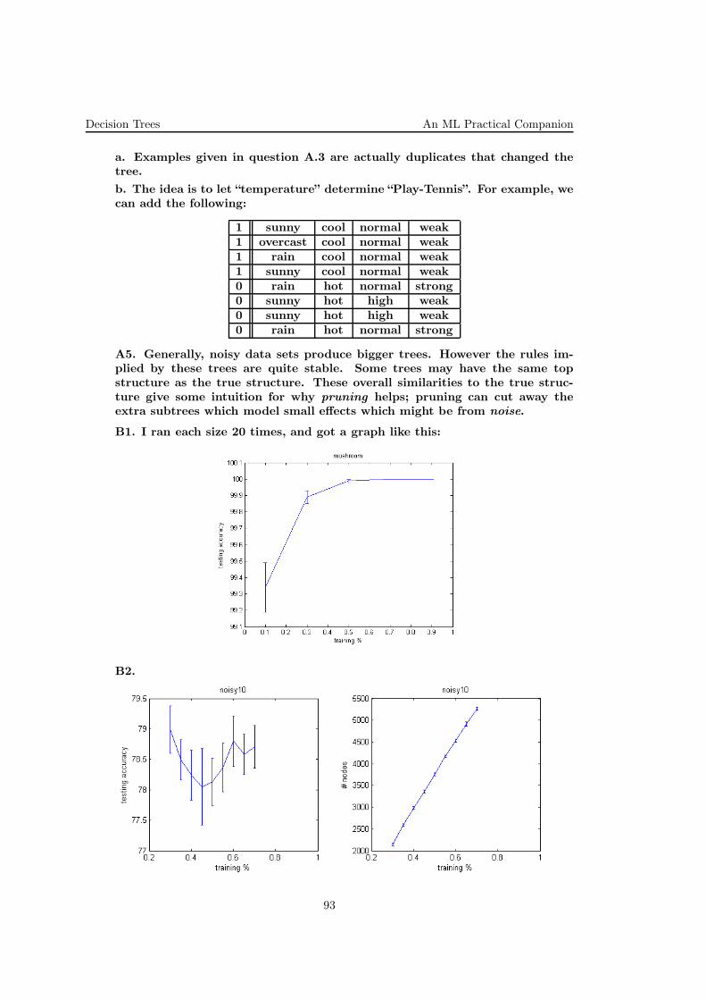
Decision Trees An ML Practical Companion
a. Examples given in question A.3 are actually duplicates that changed thetree.
b. The idea is to let “temperature” determine “Play-Tennis”. For example, wecan add the following:
1 sunny cool normal weak1 overcast cool normal weak1 rain cool normal weak1 sunny cool normal weak0 rain hot normal strong0 sunny hot high weak0 sunny hot high weak0 rain hot normal strong
A5. Generally, noisy data sets produce bigger trees. However the rules im-plied by these trees are quite stable. Some trees may have the same topstructure as the true structure. These overall similarities to the true struc-ture give some intuition for why pruning helps; pruning can cut away theextra subtrees which model small effects which might be from noise.
B1. I ran each size 20 times, and got a graph like this:
B2.
93

An ML Practical Companion Decision Trees
This decrease in testing accuracy with the larger training may be caused bya form of overfitting; that is, the algorithm tries to perfectly match the datain the training set, including the noise, and as a result the complexity ofthe learned tree increases very rapidly as the number of training examplesincreases.
Note that this is not the usual sense of overfitting, since typically overfitting ismore of a problem when the number of training examples is small. However,here we also have the problem that the complexity of the hypothesis spaceis an increasing function of the number of training examples. See how thenumber of nodes grows.
There are also “dips” in the accuracy on the test set, a point where the ac-curacy decreased before increasing again. This is because of more complexconcepts; there are always two competing forces here: the information contentof the training data, which increases with the number of training examplesand pushes toward higher accuracies, and the complexity of the hypothesisspace, which gets worse as the number of training examples increases.
You may also notice that the training accuracy slightly decreases as the sizeof the training set grows. This seems to be purely due to the noisy labels,which makes it impossible to construct a consistent tree, and the more pairsof examples you have in the training set that have contradicting labels, theworse will be the training error.
B3.
For bottom-up pruning, add to the beginning of the function:
/*******************************************************************You could insert the recursive call BEFORE you check the node
*******************************************************************/for (i = 0 ; i < node->num_children ; i++)
PruneDecisionTree(root, node->children[i], data, num_data, pruning_set, num_prune, ssvinfo);
For top-down pruning, add to the end of the function:
/*******************************************************************Or you could do the recursive call AFTER you check the node(given that you decided to keep it)
*******************************************************************/for (i = 0 ; i < node->num_children ; i++)
PruneDecisionTree(root, node->children[i], data, num_data, pruning_set, num_prune, ssvinfo);
94

Decision Trees An ML Practical Companion
By running each size 20 times I got a graph like this:
B4.
a. Bottom-up. Bottom-up pruning examines all the nodes. Top-down pruningmay eliminate a subtree without examining the nodes in the subtree, leadingto fewer calls than bottom-up.
b. Bottom-up. By the property of the algorithm, bottom-up pruning returnsthe tree with the LOWEST POSSIBLE ERROR over the pruning set. Sincetop-down can aggressively eliminate subtree’s without considering each of thenodes in the subtree, it could return a non-optimal tree (over the pruningset that is). Keep in mind that the function used to decide whether a nodeshould be removed or not is the same for both BU and TD and only the searchstrategy differs.
c. Data depedent. If the test set is very different from the training set, ashorter tree yielded by top-down pruning may perform better, because of itspotentially better generalization power.
95

An ML Practical Companion Decision Trees
35. (ID3 with continuous attributes:xxx experiment with a Matlab implementationxxx on the Breast Cancer dataset)
• CMU, 2011 fall, T. Mitchell, A. Singh, HW1, pr. 2
One very interesting application area of machine learning is in making medicaldiagnoses. In this problem you will train and test a binary decision tree todetect breast cancer using real world data. You may use any programminglanguage you like.
The Dataset
We will use the Wisconsin Diagnostic Breast Cancer (WDBC) dataset914 Thedataset consists of 569 samples of biopsied tissue. The tissue for each sampleis imaged and 10 characteristics of the nuclei of cells present in each imageare characterized. These characteristics are
(a) Radius
(b) Texture
(c) Perimeter
(d) Area
(e) Smoothness
(f) Compactness
(g) Concavity
(h) Number of concave portions of contour
(i) Symmetry
(j) Fractal dimension
Each of the 569 samples used in the dataset consists of a feature vector oflength 30. The first 10 entries in this feature vector are the mean of thecharacteristics listed above for each image. The second 10 are the standarddeviation and last 10 are the largest value of each of these characteristicspresent in each image.
Each sample is also associated with a label. A label of value 1 indicates thesample was for malignant (cancerous) tissue. A label of value 0 indicates thesample was for benign tissue.
This dataset has already been broken up into training, validation and test setsfor you and is available in the compressed archive for this problem on the classwebsite. The names of the files are trainX.csv, trainY.csv, validationX.csv,validationY.csv, testX.csv and testY.csv. The file names ending in X.csv
contain feature vectors and those ending in Y.csv contain labels. Each file isin comma separated value format where each row represents a sample.
A. Programming
A1. Learning a binary decision tree
As discussed in class and the reading material, to learn a binary decision treewe must determine which feature attribute to select as well as the threshold
914Original dataset available at http://archive.ics.uci.edu/ml/datasets/Breast+Cancer+Wisconsin+(Diagnostic).
96

Decision Trees An ML Practical Companion
value to use in the split criterion for each non-leaf node in the tree. Thiscan be done in a recursive manner, where we first find the optimal split forthe root node using all of the training data available to us. We then splitthe training data according to the criterion selected for the root node, whichwill leave us with two subsets of the original training data. We then findthe optimal split for each of these subsets of data, which gives the criterionfor splitting on the second level children nodes. We recursively continue thisprocess until the subsets of training data we are left with at a set of childrennodes are pure (i.e., they contain only training examples of one class) or thefeature vectors associated with a node are all identical (in which case we cannot split them) but their labels are different.
In this problem, you will implement an algorithm to learn the structure of atree. The optimal splits at each node should be found using the informationgain criterion discussed in class.
While you are free to write your algorithm in any language you choose, ifyou use the provided Matlab code included in the compressed archive forthis problem on the class website, you only need to complete one function,computeOptimalSplit.m. This function is currently empty and only containscomments describing how it should work. Please complete this function sothat given any set of training data it finds the optimal split according to theinformation gain criterion.
Include a printout of your completed computeOptimalSplit.m along with anyother functions you needed to write with your homework submission. If youchoose to not use the provided Matlab code, please include a printout of allthe code you wrote to train a binary decision tree according to the descriptiongiven above.
Note: While there are multiple ways to design a decision tree, in this problemwe constrain ourselves to those which simply pick one feature attribute to spliton. Further, we restrict ourselves to performing only binary splits. In otherwords, each split should simply determine if the value of a particular attributein the feature vector of a sample is less than or equal to a threshold value orgreater than the threshold value.
Note: Please note that the feature attributes in the provided dataset arecontinuously valued. There are two things to keep in mind with this.
First, this is slightly different than working with feature values which arediscrete because it is no longer possible to try splitting at every possiblefeature value (since there are an infinite number of possible feature values).One way of dealing with this is by recognizing that given a set of training dataof N points, there are only N − 1 places we could place splits for the data (ifwe constrain ourselves to binary splits). Thus, the approach you should takein this function is to sort the training data by feature value and then test splitvalues that are the mean of ordered training points. For example, if the pointsto split between were 1, 2, 3, you would test two split values: 1.5 and 2.5.
Second, when working working with feature values that can only take on oneof two values, once we split using one feature attribute, there is no point intrying to split on that feature attribute later. (Can you think of why thiswould be?) However, when working with continuously valued data, this is nolonger the case, so your splitting algorithm should consider splitting on allfeature attributes at every split.
97
An ML Practical Companion Decision Trees
A2. Pruning a binary decision tree
The method of learning the structure and splitting criterion for a binary de-cision tree described above terminates when the training examples associatedwith a node are all of the same class or there are no more possible splits.In general, this will lead to overfitting. As discussed in class, pruning is onemethod of using validation data to avoid overfitting.
You will implement an algorithm to use validation data to greedily prunea binary decision tree in an iterative manner. Specifically, the algorithmthat we will implement will start with a binary decision tree and perform anexhaustive search for the single node for which removing it (and its children)produces the largest increase (or smallest decrease) in classification accuracyas measured using validation data. Once this node is identified, it and itschildren are removed from the tree, producing a new tree. This process isrepeated, where we iteratively prune one node at a time until we are left witha tree which consists only of the root node.915
Implement a function which starts with a tree and selects the single bestnode to remove in order to produce the greatest increase (or smallest de-crease) in classification accuracy as measured with validation data. If youare using Matlab, this means you only need to complete the empty functionpruneSingleGreedyNode.m. Please see the comments in that function for de-tails on what you should implement. We suggest that you make use of theprovided Matlab functiona pruneAllNodes.m which will return a listing of allpossible trees that can be formed by removing a single node from a base treeand batchClassifyWithDT.m which will classify a set of samples given a decisiontree.
Please include your version of pruneSingleGreedyNode.m along with any otherfunctions you needed to write with your homework. If not using Matlab,please attach the code for a function which performs the same function des-cribed for pruneSingleGreedyNode.m.
B. Data analysis
B1. Training a binary decision tree
In this section, we will make use of the code that we have written above.We will start by training a basic decision tree. Please use the training dataprovided to train a decision tree. (In Matlab, assuming you have completedthe computeOptimalSplit.m function, the function trainDT.m can do this trainingfor you.)
Please specify the total number of nodes and the total number of leaf nodesin the tree. (In Matlab, the function gatherTreeStats.m will be useful.) Also,please report the classification accuracy (percent correct) of the learned deci-sion tree on the provided training and testing data. (In Matlab, the functionbatchClassifyWithDT.m will be useful.)
B2. Pruning a binary decision tree
915In practice, you can often simply continue the pruning process until the validation error fails to increase bya predefined amount. However, for illustration purposes, we will continue until there is only one node left in thetree.
98
Decision Trees An ML Practical Companion
Now we will make use of the pruning code we have written. Please startwith the tree that was just trained in the previous part of the problem andmake use of the validation data to iteratively remove nodes in the greedymanner described in the section above. Please continue iterations until adegenerate tree with only a single root node remains. For each tree thatis produced, please calculate the classification accuracy for that tree on thetraining, validation and testing datasets.
After collecting this data, please plot a line graph relating classification accu-racy on the test set to the number of leaf nodes in each tree (so number ofleaf nodes should be on the X-axis and classification accuracy should be onthe Y-Axis). Please add to this same figure, similar plots for percent accuracyon training and validation data. The number of leaf nodes should range from1 (for the degenerate tree) to the the number present in the unpruned tree.The Y-axis should be scaled between 0 and 1.
Please comment on what you notice and how this illustrates overfitting. In-clude the produced figure and any code you needed to write to produce thefigure and calculate intermediate results with your homework submission.
B3. Drawing a binary decision tree
One of the benefits of decision trees is the classification scheme they encodeis easily understood by humans. Please select the binary decision tree fromthe pruning analysis above that produced the highest accuracy on the vali-dation dataset and diagram it. (In the event that two trees have the sameaccuracy on validation data, select the tree with the smaller number of leafnodes.) When stating the feature attributes that are used in splits, pleaseuse the attribute names (instead of index) listed in the dataset section of thisproblem. (If using the provided Matlab code, the function trainDT has a sec-tion of comments which describes how you can interpret the structure usedto represent a decision tree in the code.)
Hint : The best decision tree as measured on validation data for this problemshould not be too complicated, so if drawing this tree seems like a lot of work,then something may be wrong.
B4. An alternative splitting method
While information gain is one criterion to use when estimating the optimalsplit, it is by no means the only one. Consider instead using a criterion wherewe try to minimize the weighted misclassification rate.
Formally, assume a set of D data samples < ~x(i), y(i) >Di=1, where y(i) is thelabel of sample i, and ~x(i) is the feature vector for sample i. Let x(j)(i) referto the value of the jth attribute of the feature vector for data point i.
Now, to pick a split criterion, we pick a feature attribute, a, and a thresholdvalue, t, to use in the split. Let:
pbelow(a, t) =1
D
D∑
i=1
I
(
x(a)(i) ≤ t)
pabove(a, t) =1
D
D∑
i=1
I
(
x(a)(i) > t)
99
An ML Practical Companion Decision Trees
and let:
lbelow(a, t) = Mode(
yii:x(a)(i)≤t
)
labove(a, t) = Mode(
yii:x(a)(i)>t
)
The split that minimizes the weighted misclassification rate is then the onewhich minimizes:
O(a, t) =pbelow(a, t)∑
i:x(a)(i)≤t
I
(
y(i) 6= lbelow(a, t))
+
pabove(a, t)∑
i:x(a)(i)>t
I
(
y(i) 6= labove(a, t))
Please modify the code for your computeOptimalSplit.m (or equivalent functionif not using Matlab) to perform splits according to this criterion. Attach thecode of your modified function when submitting your homework.
After modifying computeOptimalSplit.m, please retrain a decision tree (withoutdoing any pruning). In your homework submission, please indicate the totalnumber of nodes and total number of leaf nodes in this tree. How does thiscompare with the tree that was trained using the information gain criterion?
Erratum: It is important to note there is an error in question B.4, the alterna-tive splitting method. The question stated that if you minimized the equationfor O(a, t) with respect to a and t, you would find the optimal split for themisclassification rate criteria. However, this function was missing somethingimportant. The terms summing the number of samples misclassified aboveand below the split point should have been normalized. Specifically, the termsumming the number of samples misclassified above the split should have beendivided by the total number of samples above the split and the term summingthe number of samples misclassified below the split should have been dividedby the total number of samples below the split.
Solution:
B1. There are 29 total nodes and 15 leafs in the unpruned tree. The trainingaccuracy is 100% and test accuracy is 92.98%.
B2. The correct plot is shown below.
100
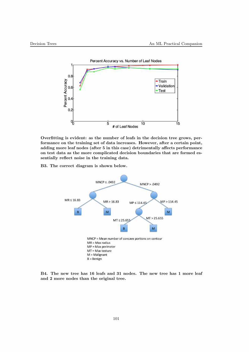
Decision Trees An ML Practical Companion
Overfitting is evident: as the number of leafs in the decision tree grows, per-formance on the training set of data increases. However, after a certain point,adding more leaf nodes (after 5 in this case) detrimentally affects performanceon test data as the more complicated decision boundaries that are formed es-sentially reflect noise in the training data.
B3. The correct diagram is shown below.
B4. The new tree has 16 leafs and 31 nodes. The new tree has 1 more leafand 2 more nodes than the original tree.
101

An ML Practical Companion Decision Trees
36. (AdaBoost: aplication on a synthetic dataset in R10)
• · CMU, ? spring (10-701), HW3, pr. 3
102

Decision Trees An ML Practical Companion
37. (AdaBoost: aplication on a synthetic dataset in R2)
• · CMU, 2016 spring, W. Cohen, N. Balcan, HW4, pr. 3.5
103
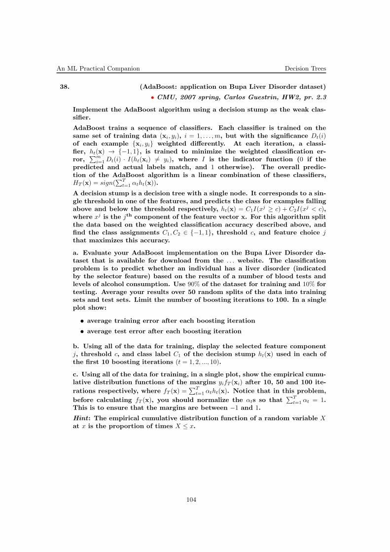
An ML Practical Companion Decision Trees
38. (AdaBoost: application on Bupa Liver Disorder dataset)
• CMU, 2007 spring, Carlos Guestrin, HW2, pr. 2.3
Implement the AdaBoost algorithm using a decision stump as the weak clas-sifier.
AdaBoost trains a sequence of classifiers. Each classifier is trained on thesame set of training data (xi, yi), i = 1, . . . ,m, but with the significance Dt(i)of each example xi, yi weighted differently. At each iteration, a classi-fier, ht(x) → −1, 1, is trained to minimize the weighted classification er-ror,
∑mi=1 Dt(i) · I(ht(xi) 6= yi), where I is the indicator function (0 if the
predicted and actual labels match, and 1 otherwise). The overall predic-tion of the AdaBoost algorithm is a linear combination of these classifiers,HT (x) = sign(
∑Tt=1 αtht(x)).
A decision stump is a decision tree with a single node. It corresponds to a sin-gle threshold in one of the features, and predicts the class for examples fallingabove and below the threshold respectively, ht(x) = C1I(x
j ≥ c) + C2I(xj < c),
where xj is the jth component of the feature vector x. For this algorithm splitthe data based on the weighted classification accuracy described above, andfind the class assignments C1, C2 ∈ −1, 1, threshold c, and feature choice jthat maximizes this accuracy.
a. Evaluate your AdaBoost implementation on the Bupa Liver Disorder da-taset that is available for download from the . . . website. The classificationproblem is to predict whether an individual has a liver disorder (indicatedby the selector feature) based on the results of a number of blood tests andlevels of alcohol consumption. Use 90% of the dataset for training and 10% fortesting. Average your results over 50 random splits of the data into trainingsets and test sets. Limit the number of boosting iterations to 100. In a singleplot show:
• average training error after each boosting iteration
• average test error after each boosting iteration
b. Using all of the data for training, display the selected feature componentj, threshold c, and class label C1 of the decision stump ht(x) used in each ofthe first 10 boosting iterations (t = 1, 2, ..., 10).
c. Using all of the data for training, in a single plot, show the empirical cumu-lative distribution functions of the margins yifT (xi) after 10, 50 and 100 ite-
rations respectively, where fT (x) =∑T
t=1 αtht(x). Notice that in this problem,
before calculating fT (x), you should normalize the αts so that∑T
t=1 αt = 1.This is to ensure that the margins are between −1 and 1.
Hint : The empirical cumulative distribution function of a random variable Xat x is the proportion of times X ≤ x.
104
Decision Trees An ML Practical Companion
39. (AdaBoost (basic, and randomized decision stumps versions):xxx application to high energy physics)
• Stanford, 2016 fall, A. Ng, J. Duchi, HW2, pr. 6.d
In this problem, we apply [two versions of the] AdaBoost algorithm to de-tect particle emissions in a high-energy particle accelerator. In high energyphysics, such as at the Large Hadron Collider (LHC), one accelerates smallparticles to relativistic speeds and smashes them into one another, trackingthe emitted particles. The goal is to detect the emission of certain interestingparticles based on other observed particles and energies.916 Here we explorethe application of boosting to a high energy physics problem, where we usedecision stumps applied to 18 low- and high-level physics-based features. Alldata for the problem is available at ....
You will implement AdaBoost using decision stumps and run it on data deve-loped from a physics-based simulation of a high-energy particle accelerator.
We provide two datasets, boosting-train.csv and boosting-test.csv, whichconsist of training data and test data for a binary classification problem. Thefiles are comma-separated files, the first column of which consists of binary±1-labels y(i), the remaining 18 columns are the raw attribtues (low- and high-level physics-based features).
The MatLab file load_data.m, which we provide, loads the datasets into me-mory, storing training data and labels in appropriate vectors and matrices, andthen performs boosting using your implemented code, and plots the results.
a. Implement a method that finds the optimal thresholded decision stumpfor a training set x(i), y(i)mi=1 and distribution p ∈ R
m+ on the training set. In
particular, fill out the code in the method find_best_threshold.m.
b. Implement boosted decision stumps by filling out the code in the methodstump_booster.m. Your code should implement the weight updating at eachiteration t = 1, 2, . . . to find the optimal value θt given the feature index andthreshold.
c. Implement random boosting, where at each step the choice of decision stumpis made completely randomly. In particular, at iteration t random boostingchooses a random index j ∈ 1, 2, . . . , n, then chooses a random threshold
s from among the data values x(i)j mi=1, and then chooses the t-th weight θt
optimally for this (random) classifier φs,+(x) = sign(xj − s). Implement this byfilling out the code in random_booster.m.
d. Run the method load data.m with your implemented boosting methods.Include the plots this method displays, which show the training and test errorfor boosting at each iteration t = 1, 2, . . .. Which method is better?
[A few notes: we do not expect boosting to get classification accuracy betterthan approximately 80% for this problem.]
Solution:
916For more information, see the following paper: Baldi, Sadowski, Whiteson. Searching for Exo-tic Particles in High-Energy Physics with Deep Learning. Nature Communications 5, Article 4308.http://arxiv.org/abs/1402.4735.
105
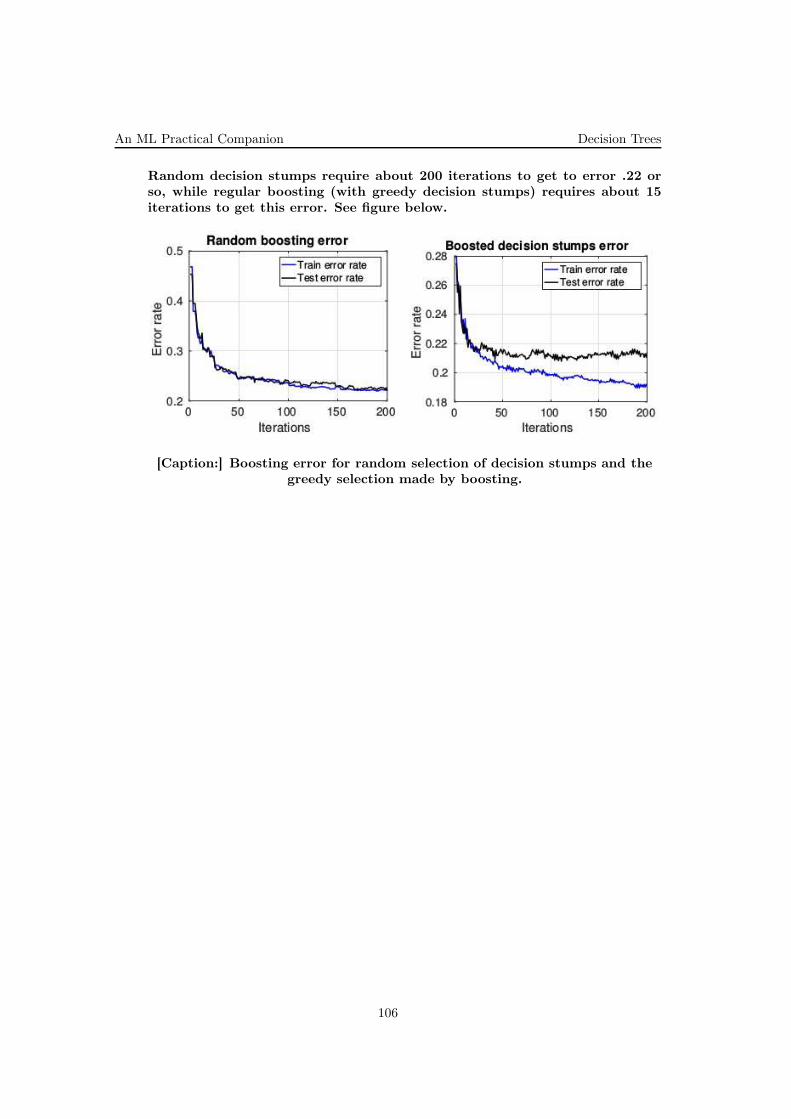
An ML Practical Companion Decision Trees
Random decision stumps require about 200 iterations to get to error .22 orso, while regular boosting (with greedy decision stumps) requires about 15iterations to get this error. See figure below.
[Caption:] Boosting error for random selection of decision stumps and thegreedy selection made by boosting.
106
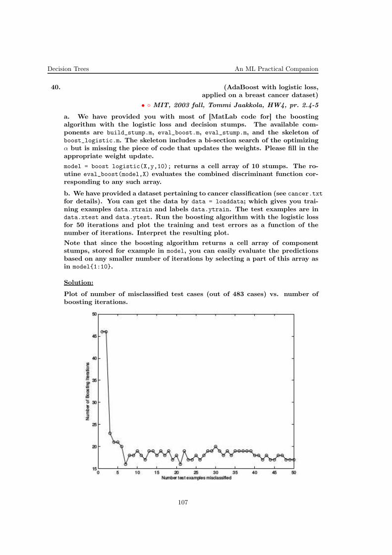
Decision Trees An ML Practical Companion
40. (AdaBoost with logistic loss,xxx applied on a breast cancer dataset)
• MIT, 2003 fall, Tommi Jaakkola, HW4, pr. 2.4-5
a. We have provided you with most of [MatLab code for] the boostingalgorithm with the logistic loss and decision stumps. The available com-ponents are build_stump.m, eval_boost.m, eval_stump.m, and the skeleton ofboost_logistic.m. The skeleton includes a bi-section search of the optimizingα but is missing the piece of code that updates the weights. Please fill in theappropriate weight update.
model = boost logistic(X,y,10); returns a cell array of 10 stumps. The ro-utine eval_boost(model,X) evaluates the combined discriminant function cor-responding to any such array.
b. We have provided a dataset pertaining to cancer classification (see cancer.txt
for details). You can get the data by data = loaddata; which gives you trai-ning examples data.xtrain and labels data.ytrain. The test examples are indata.xtest and data.ytest. Run the boosting algorithm with the logistic lossfor 50 iterations and plot the training and test errors as a function of thenumber of iterations. Interpret the resulting plot.
Note that since the boosting algorithm returns a cell array of componentstumps, stored for example in model, you can easily evaluate the predictionsbased on any smaller number of iterations by selecting a part of this array asin model1:10.
Solution:
Plot of number of misclassified test cases (out of 483 cases) vs. number ofboosting iterations.
107
An ML Practical Companion Decision Trees
41. (AdaBoost with confidence rated decision stumps;xxx application to handwritten digit recognition;xxx analysis of the evolution of voting margins)
• MIT, 2001 fall, Tommi Jaakkola, HW3, pr. 1.4
Let’s explore how AdaBoost behaves in practice. We have provided you withMatLab code that finds and evaluates (confidence rated) decision stumps.917
These are the hypothesis that our boosting algorithm assumes we can ge-nerate. The relevant Matlab files are boost_digit.m, boost.m, eval_boost.m,find_stump.m, eval_stump.m. You’ll only have to make minor modificationsto boost.m and, a bit later, to eval_boost.m and boost digit.m to make thesework.
a. Complete the weight update in boost.m and run boost_digit to plot thetraining and test errors for the combined classifier as well as the correspondingtraining error of the decision stump, as a function of the number of iterations.Are the errors what you would expect them to be? Why or why not?
We will now investigate the classification margins of training examples. Re-call that the classification margin of a training point in the boosting contextreflects the “confidence” in which the point was classified correctly. You canview the margin of a training example as the difference between the weightedfraction of votes assigned to the correct label and those assigned to the incor-rect one. Note that this is not a geometric notion of “margin” but one basedon votes. The margin will be positive for correctly classified training pointsand negative for others.
b. Modify eval boost.m so that it returns normalized predictions (normalizedby the total number of votes). The resulting predictions should be in the range[−1, 1]. Fill in the missing computation of the training set margins in boost
digit.m (that is, the classification margins for each of the training points). Youshould also uncomment the plotting script for cumulative margin distributions(what is plotted is, for each −1 < r < 1 on the horizontal axis, what fractionof the training points have a margin of at least r). Explain the differencesbetween the cumulative distributions after 4 and 16 boosting iterations.
Solution:
917LC: For some theoretical properties of confidence rated [weak] classifiers [when used] in connection withAdaBoost, see MIT, 2001 fall, Tommi Jaakkola, HW3, pr. 2.1-3.
108

Decision Trees An ML Practical Companion
a.
As can be seen in the figure, the training and test errors decrease as weperform more boosting iterations. Eventually the training error reaches zero,but we do not overfit, and the test error remains low (though higher than thetraining error). However, no single stump can predict the training set well,and especially since we continue to emphasize “difficult” parts of the trainingset, the error of each particular stump remains high, and does not drop bellowabout 1/3.
b.
The key difference between the cumulative distributions after 4 and 16 bo-osting iterations is that the additional iterations seem to push the left (lowend) tail of the cumulative distribution to the right. To understand the effect,
109

An ML Practical Companion Decision Trees
note that the examples that are difficult to classify have poor or negativeclassification margins and therefore define the low end tail of the cumulativedistribution. Additional boosting iterations concentrate on the difficult exam-ples and ensure that their margins will improve. As the margins improve, theleft tail of the cumulative distribution moves to the right, as we see in thefigure.
110
Decision Trees An ML Practical Companion
42. (AdaBoost with logistic loss:xxx studying the evolution of voting marginsxxx as a function of boosting iterations)
• MIT, 2009 fall, Tommi Jaakkola, HW3, pr. 2.4
We have provided you with MatLab code that you can run to test how Ada-Boost works.mod = boost(X,y,ncomp) generates an ensemble (a cell array of ncomp base lear-ners) based on training examples X and labels y.load data.mat gives you X and y for a simple classification task. You canthen generate the ensemble with any number of components (e.g., 50). Thecell array mod simply lists the base learners in the order in which they werefound. You can therefore plot the ensemble corresponding to the first i
base learners by plot_decision(mod(1:i),X,y), or individual base learners viaplot_decision(modi,X,y).
plot_voting_margin(mod,X,y,th)helps you study how the voting margins changeas a function of boosting iterations. For example, the plot with th = 0 givesthe fraction of correctly classified training points (voting margin > 0) as afunction of boosting iterations. You can also plot the curves for multiplethresholds at once as in plot_voting_margin(mod,X,y,[0,0.05,0.1,0.5]). Ex-plain why some of these tend to increase while others decrease as a functionof boosting iterations. Why does the curve corresponding to th = 0.05 conti-nue to increase even after all the points are correctly classified?
Solution:
Let hm(x) =∑m
i=1 αihi(x) denote the ensemble classifier after m boosting ite-
rations, and let hm(x) =
∑mi=1 αihi(x)∑m
i=1 αibe its normalized version. Let f(τ,m)
denote the fraction of training examples (xt, yt) with voting margin ythm(xt) =ythm(xt)∑m
i=1 αi> τ . From our plot, we notice that f(τ,m) is increasing with m (quite
roughly and not at all monotonically) for small values of τ , like τ = 0, 0.05, 0.1,but decreasing for large values of τ , like τ = 0.5. (The threshold at which thetransition occurs seems to be somewhere in the interval 0.115 > τ > 0.105.)
To explain this, consider the boosting loss function, Jm =∑n
t=1 L(yt hm(xt)),
which is decreasing in the voting margins ythm(xt). To minimize Jm, AdaBoostwill try to make all the voting margins yhm(xt) as positive as possible. As m
increases,∑m
i=1 αi only grows, so a negative voting margin ythm(xt) < 0 onlybecomes more costly. So, after a sufficient number of iterations, we know thatboosting will be able to classify all points correctly, and all points will havepositive voting margin. So, f(0,m) roughly increases from 0.5 to 1, and staysat 1 once m is sufficiently large.
As m increases even more, we should expect that the minimum voting marginmint yth(xt) continues to increase. This is because there is little incentive tomake the larger ythm(xt) any more positive; it is more effective to make thesmaller ythm(xt) more positive. Using an argument similar to the one frompart a of this problem (MIT, 2009 fall, T. Jaakkola, HW3, pr. 2.1), we canshow that the examples which are barely correct have larger weight (Wm(t))than the examples which are clearly correct, since dL(z) is larger near 0.
111

An ML Practical Companion Decision Trees
However, our decision stumps are fairly weak classifiers. If we want to per-form better on some subset of points (namely, the ones with smaller margin),we must compromise on the rest (namely, the ones with larger margin). Thus,what we get is that the minimum voting margin (which costs more) will be-come larger at the expense of the maximum voting margin (which costs less).Similarly, f(τ, n) for a small threshold τ will increase at the expense of f(τ, n)for a large τ .
A visual way to see this is to consider a graph of the rescaled loss functionL((∑m
i=1 αi)τ) vs. the voting margin τ = ythm(xt). As the number of boostingiterations increases, the graph is compressed along the horizontal axis (altho-ugh increasingly slowly). So to make Jm smaller, we must basically shift theentire distribution of voting margins to the right as much as possible (tho-ugh we can only do so increasingly slowly). In doing this, we are forced tocompromise some of the points farthest to the right, moving them inward.Thus, with more iterations, the distribution of margins narrows. Here, f(τ, n)can be related to the cumulative density on the empirical distribution of vo-ting margins. So, f(τ, n) = P (margin > τ) for a small τ will increase, while1 − f(τ, n) = P (margin < τ) for large τ will also increase (or at least be non-decreasing).
[Caption:] Voting Margins, 10-20 iterations.
112
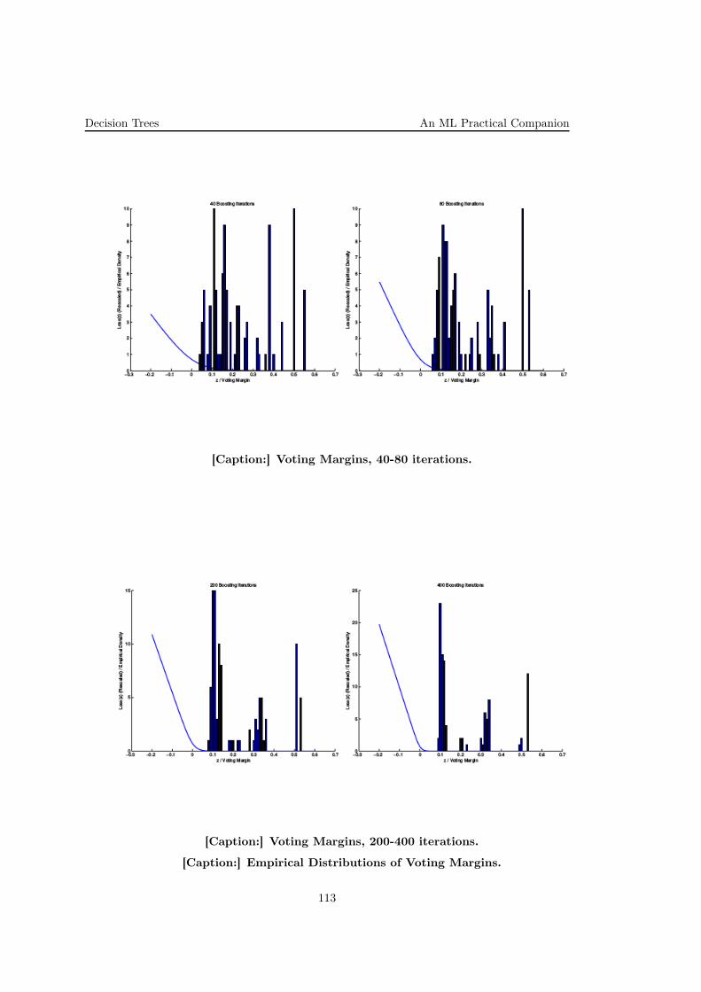
Decision Trees An ML Practical Companion
[Caption:] Voting Margins, 40-80 iterations.
[Caption:] Voting Margins, 200-400 iterations.
[Caption:] Empirical Distributions of Voting Margins.
113

An ML Practical Companion Decision Trees
-0.5 0 0.5
-0.8
-0.6
-0.4
-0.2
0
0.2
0.4
0.6
0.8
-0.5 0 0.5
-0.8
-0.6
-0.4
-0.2
0
0.2
0.4
0.6
0.8
[Caption:] Decision boundaries, 10-20 iterations.
-0.5 0 0.5
-0.8
-0.6
-0.4
-0.2
0
0.2
0.4
0.6
0.8
-0.5 0 0.5
-0.8
-0.6
-0.4
-0.2
0
0.2
0.4
0.6
0.8
[Caption:] Decision boundaries, 40-80 iterations.
114
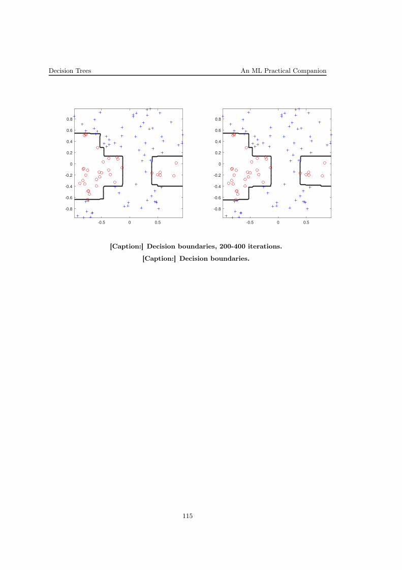
Decision Trees An ML Practical Companion
-0.5 0 0.5
-0.8
-0.6
-0.4
-0.2
0
0.2
0.4
0.6
0.8
-0.5 0 0.5
-0.8
-0.6
-0.4
-0.2
0
0.2
0.4
0.6
0.8
[Caption:] Decision boundaries, 200-400 iterations.
[Caption:] Decision boundaries.
115
An ML Practical Companion Decision Trees
43. (Liniear regression vs.xxx AdaBoost using [weighted] linear weak classifiersxxx and mean square error as loss function;xxx cross-validation;xxx application on the Wine dataset)
• CMU, 2009 spring, Ziv Bar-Joseph, HW3, pr. 1
In this problem, you are going to compare the performance of a basic linearclassifier and its boosted version on the Wine dataset (available on our web-site). The dataset, given in the file wine.mat, contains the results of a chemicalanalysis of wines grown in the same region in Italy but derived from threedifferent cultivars. The analysis determined the quantities of 13 constituentsfound in each of the three types of wines. Note that when you are doingcross-validation, you want to ensure that across all the folds the proportionexamples from each class is roughly the same.
a. Implement a basic linear classifier using linear regression. All data pointsare equally weighted.
A linear classifier is defined as:
f(x;β) = sign(β⊤ · x) =
−1 if β⊤ · x < 0;1 if β⊤ · x ≥ 0.
Your algorithm should minimize the classification error defined as:
err(f) =
n∑
i=1
(yi − f(xi))2
4n
Note: The first step for data preprocessing is to augment the data. In MatLab,this can be done as:
X_new = [ones(size(X,1), 1) X];
Hint : You may want to use the MatLab function fminsearch to get the optimalsolution for β.
Handin : Please turn in a MatLab source file linear_learn.m which takes intwo inputs data matrix x and label y, and returns a linear model. You mayhave additional functions/files if you want.
b. Do 10-fold cross validation for the linear classifier. Report the averagetraining and test errors for all the folds.
Handin : Please turn in a MatLab source file cv.m.
c. Modify your algorithm in linear_learn.m to accommodate weighted sam-ples. Given the weight w for sample data X, what is the classification error?You may want to refer to part a. Please implement the weighted version ofthe learning algorithm for the linear classifier.
Note originally the unweighted version could be viewed as one with equalweights 1/n.
Handin : Please turn in a MatLab source file linear_learn.m which takes inthree inputs data matrix x, label y and weights w, and returns a linear model.You may have additional functions/files if you want. Note that your code
116
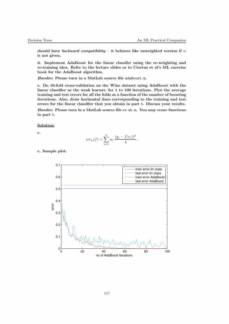
Decision Trees An ML Practical Companion
should have backward compatibility – it behaves like unweighted version if wis not given.
d. Implement AdaBoost for the linear classifer using the re-weighting andre-training idea. Refer to the lecture slides or to Ciortuz et al’s ML exercisebook for the AdaBoost algorithm.
Handin : Please turn in a MatLab source file adaBoost.m.
e. Do 10-fold cross-validation on the Wine dataset using AdaBoost with thelinear classifier as the weak learner, for 1 to 100 iterations. Plot the averagetraining and test errors for all the folds as a function of the number of boostingiterations. Also, draw horizontal lines corresponding to the training and testerrors for the linear classifier that you obtain in part b. Discuss your results.
Handin : Please turn in a MatLab source file cv ab.m. You may reuse functionsin part b.
Solution:
c.
errw(f) =
n∑
i=1
wi(yi − f(xi))
2
4.
e. Sample plot:
0 20 40 60 80 1000
0.1
0.2
0.3
0.4
0.5
0.6
0.7
no of AdaBoost iterations
err
or
train error lin class
test error lin class
train error AdaBoost
test error AdaBoost
117

An ML Practical Companion Decision Trees
44. (AdaBoost using Naive Bayes as weak classifier;xxx application on the US House of Representatives votes dataset)
• CMU, 2005 spring, C. Guestrin, T. Mitchell, HW2, pr. 1.2
Solution:
118
Support Vector Machines An ML Practical Companion
5 Support Vector Machines
45. (An implementation of SVM using the quadprog MatLab function;xxx application on different datasets from R
2)
• · MIT, 2001 fall, Tommi Jaakkola, HW3, pr. 2
46. (Choosing an SVM kernel)
• · CMU, 2013 fall, A. Smola, B. Poczos, HW3, pr. 2
47. (An implementation of SVM using the quadprog MatLab function;xxx comparison with the perceptron;xxx using SVMlight for digit recognition)
• · MIT, 2006 fall, Tommi Jaakkola, HW1, section B
48. (ν-SVM: implementation using the quadprog MatLab function;xxx train and test it on a given dataset)
• · MIT, 2004 fall, Tommi Jaakkola, HW3, pr. 3.3
49. (Minimum Enclosing Ball (MEB) / Anomaly detection)
• · MIT, 2009 fall, Tommi Jaakkola, HW2, pr. 2.cd
• CMU, 2017 fall, Nina Balcan, HW4, pr. 4.1
Let S = (x1, y1), . . . (xn, yn) be n labeled examples in Rd with label set 1,−1.
Recall that the primal formulation of SVM is given by
Primal
minw∈Rd,ξ1,...ξn
‖w‖2 + Cn∑
i=1
ξi,
s.t. ∀i, yi 〈w,Xi〉 ≥ 1− ξi, ξi ≥ 0.
It can be proven (see ex. 21) that the primal problem can be rewritten asthe following equivalent problem in the Empirical Risk Minimization (ERM)framework
minw∈Rd
λ‖w‖22 +1
n
n∑
i=1
max(1 − yi 〈w,Xi〉 , 0), (361)
where λ = 1nC .
We will now optimize the above unconstrained formulation of SVM using Sto-chastic Sub-Gradient Descent. In this problem you will be using a binary (two
119
An ML Practical Companion Support Vector Machines
class) version of mnist dataset. The data and code template can be downloa-ded from the class website:https://sites.google.com/site/10715advancedmlintro2017f/homework-exams.The data folder has mnist2.mat file which contains the train, test and valida-tion datasets. The python folder has python code template (and matlab folderhas the matlab code template) which you will use for your implementation.You can either use python or matlab for this programming question.
We slightly modify Equation (361) and use the following formulation in thisproblem
minw∈Rd
λ
2‖w‖22 +
1
n
n∑
i=1
max(1 − yi 〈w,Xi〉 , 0).
This is only done to simplify calculations. You will optimize this objectiveusing Stochastic Sub-Gradient Descent (SSGD).918 This approach is very sim-ple and scales well to large datasets.919 In SSGD we randomly sample atraining data point in each iteration and update the weight vector by takinga small step along the direction of negative “sub-gradient” of the loss.920
The SSGD algorithm is given by
• Initialize the weight vector w = 0.
• For t = 1 . . . T
* Choose it ∈ 1, . . . n uniformly at random
* Set ηt =1λt .
* If yit 〈w,Xit〉 < 1 then:
– Set w ← (1− ληt)w + ηtyitXit
* Else:
– Set w ← (1− ληt)w
• Return w
Note that we don’t consider the bias/intercept term in this problem.
a. Complete the train(w0, Xtrain, ytrain, T, lambda) function in the svm.py
file (matlab users complete the train.m file).
b. The function train(w0, Xtrain, ytrain, T, lambda) runs the SSGD algo-rithm, taking in an initial weight vector w0, matrix of covariates Xtrain, avector of labels ytrain. T is the number of iterations of SSGD and lambda isthe hyper-parameter in the objective. It outputs the learned weight vector w.
c. Run svm_run.py to perform training and see the performance on trainingand test sets.
d. Use validation dataset for picking a good lambda(λ) from the set 1e3,
1e2, 1e1, 1, 0.1.
918See Shai Shalev-Shwartz, Yoram Singer, Nathan Srebro, and Andrew Cotter. Pegasos: Primal estimated
sub-gradient solver for SVM. Mathematical programming, 127(1):3-30, 2011.919To estimate optimal w, one can also optimize the dual formulation of this problem. Some of the popular
SVM solvers such as LIBSVM solve the dual problem. Other fast approaches for solving dual formulation onlarge datasets use dual coordinate descent.920Sub-gradient generalizes the notion of gradient to non-differentiable functions.
120

Support Vector Machines An ML Practical Companion
e. Report the accuracy numbers on train and test datasets obtained using thebest lambda, after running SSGD for 200 epochs (i.e., T = 200 ∗ n). Generatethe training accuracy vs. training time and test accuracy vs training timeplots.
121

An ML Practical Companion Artificial Neural Networks
6 Artificial Neural Networks
50. (Reţele neuronale: chestiuni de bază)
• MPI, 2005 spring, Jörg Rahnenfuhrer, Adrian Alexa, HW2, pr. 5
a. Simulate data by randomly drawing two-dimensional data points uniformlydistributed in [0, 1]2. The class Y of a sample X = (X1, X2) is 1 if X1 +X2 > 1and −1 otherwise. You can add some noise to the data by using the ruleX1 +X2 > 1 + ε with ε ∼ N (0, 0.1). Use 100 samples for the training set (youcan use training data with or without noise).
b. Write a function to train a perceptron for a two class classification problem.A perceptron is a classifier which constructs a linear decision boundary thattries to separate the data into different classes as best as possible. Section 4.5.1in The Elements of Statistical Learning book by Hastie, Tibshirani, Friedmandescribes how the perceptron learning algorithm works.
c. Write a function to predict the class for new data points. Write a functionthat performs LOOCV (Leave-One-Out Cross-Validation) for your classifier.Use these functions to estimate the train error and the the prediction er-ror. Generate a test set of 1000 samples and compute the test error of yourclassifier.
d. Use the data generator xor.data() from the tutorial homepage to generatea new training (ca. 100 samples) and test set (ca. 1000 samples). Train theperceptron on this data. Report the train and test errors. Plot the testsamples to see how they are classified by the perceptron.
e. Comment your findings. Is the perceptron able to learn the XOR data?What is the main difference between the data generated in part a and thedata from part d?
f. Use the nnet R package to train a neural network for the XOR data. Thennet() function is fitting a neural network. Use the predict() function to assesthe train and test errors.
h. Vary the number of units in the hidden layer and report the train and testerrors. We have seen at part e that a perceptron, a neural network with nounit in the hidden layer can not correctly classify the XOR data. Argue whichis the minimal number of units in the hidden layer that a neural network musthave to correctly classify the XOR data. Train such a network and report thetrain, prediction and test errors.
122
Artificial Neural Networks An ML Practical Companion
51. (The Perceptron algorithm:xxx spam identification)
• New York University, 2016 spring, David Sontag, HW1
In this problem set you will implement the Perceptron algorithm and applyit to the problem of e-mail spam classification.
Instructions. You may use the programming language of your choice (werecommend Python, and using matplotlib for plotting). However, you arenot permitted to use or reference any machine learning code or packages notwritten by yourself.
Data files. We have provided you with two files: spam train.txt, and spam
test.txt. Each row of the data files corresponds to a single email. The firstcolumn gives the label (1=spam, 0=not spam).
Pre-processing. The dataset included for this exercise is based on a subset ofthe SpamAssassin Public Corpus. Figure 1 shows a sample email that containsa URL, an email address (at the end), numbers, and dollar amounts. Whilemany emails would contain similar types of entities (e.g., numbers, otherURLs, or other email addresses), the specific entities (e.g., the specific URL orspecific dollar amount) will be different in almost every email. Therefore, onemethod often employed in processing emails is to “normalize” these values,so that all URLs are treated the same, all numbers are treated the same,etc. For example, we could replace each URL in the email with the uniquestring “httpaddr” to indicate that a URL was present. This has the effectof letting the spam classifier make a classification decision based on whetherany URL was present, rather than whether a specific URL was present. Thistypically improves the performance of a spam classifier, since spammers oftenrandomize the URLs, and thus the odds of seeing any particular URL againin a new piece of spam is very small.
We have already implemented the following email preprocessing steps: lower-casing; removal of HTML tags; normalization of URLs, e-mail addresses, andnumbers. In addition, words are reduced to their stemmed form. For example,“discount”, “discounts”, “discounted” and “discounting” are all replaced with“discoun. Finally, we removed all non-words and punctuation. The result ofthese preprocessing steps is shown in Figure 2.
Figure 1: Sample e-mail in SpamAssassin corpus before pre-processing.> Anyone knows how much it costs to host a web portal?> Well, it depends on how many visitors youre expecting. This can beanywhere from less than 10 bucks a month to a couple of $100. You sho-uld checkout http://www.rackspace.com/ or perhaps Amazon EC2 if yourerunning something big.To unsubscribe yourself from this mailing list, send an email to: groupname-unsubscribeegroups.com.
Figure 2: Pre-processed version of the sample e-mail from Figure 1.anyon know how much it cost to host a web portal well it depend on how manivisitor your expect thi can be anywher from less than number buck a monthto a coupl of dollarnumb you should checkout httpaddr or perhap amazonecnumb if your run someth big to unsubscrib yourself from thi mail list sendan email to emailaddr
123

An ML Practical Companion Artificial Neural Networks
a. This problem set will involve your implementing several variants of thePerceptron algorithm. Before you can build these models and measure theirperformance, split your training data (i.e. spam_train.txt) into a trainingand validation set, putting the last 1000 emails into the validation set. Thus,you will have a new training set with 4000 emails and a validation set with1000 emails. You will not use spam_test.txt until problem j. Explain whymeasuring the performance of your final classifier would be problematic hadyou not created this validation set.
b. Transform all of the data into feature vectors. Build a vocabulary list usingonly the 4000 e-mail training set by finding all words that occur across thetraining set. Note that we assume that the data in the validation and testsets is completely unseen when we train our model, and thus we do not useany information contained in them. Ignore all words that appear in fewerthan X = 30 e-mails of the 4000 e-mail training set – this is both a means ofpreventing overfitting and of improving scalability. For each email, transformit into a feature vector x where the ith entry, xi, is 1 if the ith word in thevocabulary occurs in the email, and 0 otherwise.
c. Implement the functions perceptron_train(data) and perceptron_test(w,
data).The function perceptron_train(data) trains a perceptron classifier using theexamples provided to the function, and should return w, k, and iter, the finalclassification vector, the number of updates (mistakes) performed, and thenumber of passes through the data, respectively. You may assume that theinput data provided to your function is linearly separable (so the stoppingcriterion should be that all points are correctly classified). For the cornercase of w · x = 0, predict the +1 (spam) class.For this exercise, you do not need to add a bias feature to the feature vector (itturns out not to improve classification accuracy, possibly because a frequentlyoccurring word already serves this purpose). Your implementation shouldcycle through the data points in the order as given in the data files (ratherthan randomizing), so that results are consistent for grading purposes.The function perceptron_test(w, data) should take as input the weight vectorw (the classification vector to be used) and a set of examples. The functionshould return the test error, i.e. the fraction of examples that are misclassifiedby w.
d. Train the linear classifier using your training set. How many mistakesare made before the algorithm terminates? Test your implementation ofperceptron_test by running it with the learned parameters and the trainingdata, making sure that the training error is zero. Next, classify the emails inyour validation set. What is the validation error?
e. To better understand how the spam classifier works, we can inspect theparameters to see which words the classifier thinks are the most predictive ofspam. Using the vocabulary list together with the parameters learned in theprevious question, output the 15 words with the most positive weights. Whatare they? Which 15 words have the most negative weights?
f. Implement the averaged perceptron algorithm, which is the same as yourcurrent implementation but which, rather than returning the final weight vec-tor, returns the average of all weight vectors considered during the algorithm
124

Artificial Neural Networks An ML Practical Companion
(including examples where no mistake was made). Averaging reduces the va-riance between the different vectors, and is a powerful means of preventingthe learning algorithm from overfitting (serving as a type of regularization).
g. One should expect that the test error decreases as the amount of trainingdata increases. Using only the first N rows of your training data, run both theperceptron and the averaged perceptron algorithms on this smaller trainingset and evaluate the corresponding validation error (using all of the validationdata). Do this for N = 100, 200, 400, 800, 2000, 4000, and create a plot of thevalidation error of both algorithms as a function of N .
h. Also for N = 100, 200, 400, 800, 2000, 4000, create a plot of the number of per-ceptron iterations as a function of N , where by iteration we mean a completepass through the training data. As the amount of training data increases, themargin of the training set decreases, which generally leads to an increase inthe number of iterations perceptron takes to converge (although it need notbe monotonic).
i. One consequence of this is that the later iterations typically perform updateson only a small subset of the data points, which can contribute to overfitting.A way to solve this is to control the maximum number of iterations of theperceptron algorithm. Add an argument to both the perceptron and averagedperceptron algorithms that controls the maximum number of passes over thedata.
j. Congratulations, you now understand various properties of the perceptronalgorithm. Try various configurations of the algorithms on your own using all4000 training points, and find a good configuration having a low error on yourvalidation set. In particular, try changing the choice of perceptron algorithmand the maximum number of iterations. You could additionally change Xfrom question b (this is optional). Report the validation error for several ofthe configurations that you tried; which configuration works best?You are ready to train on the full training set, and see if it works on comple-tely new data. Combine the training set and the validation set (i.e. use allof spam_train.txt) and learn using the best of the configurations previouslyfound. You do not need to rebuild the vocabulary when re-training on thetrain+validate set.What is the error on the test set (i.e., now you finally use spam test.txt)?
Note: This problem set is based partly on an assignment developed by AndrewNg of Stanford University and Coursera.
125

An ML Practical Companion Artificial Neural Networks
52. (The backpropagation algorithm:xxx application on the Breast Cancer dataset)
• MPI, 2005 spring, Jörg Rahnenfuhrer, Adrian Alexa, HW2, pr. 6
Download the breast cancer data set breastcancer.zip from the tutorial ho-mepage. The data are described in Mike West et al.: Predicting the clini-cal status of human breast cancer by using gene expression profiles, PNAS98(20):11462-11467, 2001. The file contains expression profiles of 46 patientsfrom two different classes: 23 patients are estrogen receptor positive (ER+)and 23 are estrogen receptor negative (ER-). For every patient, the expres-sion values of 7129 genes were measured. Use the nnet R package to train aneural network.
a. Load breastcancer.Rdata and apply summary() to get an overview of thisdata object: breastcancer$x contains the expression data and breastcancer$y
the class labels. Reformat the data by transposing the gene expression matrixand renaming the classes ER+, ER− to +1,−1.b. Train a Neural Network using the nnet() function. Check if the inputs arestandardized (mean zero and standard deviation one) and if this is not thecase, standardize them.
c. Apply the function predict() to the training data and calculate the trai-ning error. Perform a LOOCV to estimate the prediction error (you mustimplement by yourself the cross validation procedure).
d. Predict the classes of the three new patients (newpatients). The true classlabels are stored in (trueclasses). Are they correctly classified?
e. Try different parameters in the nnet() function (the number of units in thehidden layer, the weights, the activation function, the weight decay parame-ter, etc.) and report the parameters for which you obtained the best result.Comment the way the parameters affect the performance of the network.
126

Artificial Neural Networks An ML Practical Companion
53. (Artificial neural networks:xxx Digit classification competition)
• CMU, 2014 fall, William Cohen, Ziv Bar-Joseph, HW3
In this section, you are asked to construct a neural network using a datasetin real world. The training samples and training labels are provided in thehandout folder. Each sample is a 28×28 gray scale image. Each pixel (feature)is a real value between 0 and 1 denoting the pixel intensity. Each label is ainteger from 0 to 9 which corresponds to the digit in the image.
A. Getting Started
Getting Familiar with Data
As mentioned above, each sample is an image with 784 pixels. Load the datausing the following command:load(‘digits.mat’)
Visualize an image using the following command:imshow(vec2mat(XTrain(i,:),28)’)
where X ∈ Rn×784 is the training samples; i is the row index of a training
sample.
Neural Network Structure
In this competition, you are free to use any neural network structure. A simplefeed forward neural network with one hidden layer is shown in Figure... . Theinput layer has a bias neuron and 784 neurons with each corresponding to onepixel in the image. The output layer has 10 neurons with each representingthe probability of each digit given the image. You need to decide the size ofthe hidden layer.
Code Structure
You should implement your training algorithm (typically the forward pro-pagation and back propagation) in train_ann.m and testing algorithm (usingtrained weights to predict labels) in test_ann.m. In your training algorithm,you need to store your initial and final weights into a mat file. In the simpleexample below, two weight matrices Wih and Who are stored into weights.mat:save(‘weights.mat’,‘Wih’,‘Who’);
Be sure your test ann.m runs fast enough. It is always good to vectorize yourcode in Matlab.
Separating Data
Digits.mat contains 3000 instances which you used in previous section. Thenumber of instances are pretty balanced for each digit so you do not need toworry about skewness of the data. However, you need to handle the overfittingproblem. Neural networks are very powerful models which are capable toexpress extremely complicated functions but very prone to overfit.
The standard approach for building a model on a dataset can be described asfollows:
• Divide your data into three sets: a training set, a validation set, a testset. You can use any sizes for three sets as long as they are reasonable(e.g. 60%, 20%, 20%). You can also combine the training set and thevalidation set and do k-fold cross-validation. Make sure to have balancednumbers of instances for each class in every set.
127

An ML Practical Companion Artificial Neural Networks
• Train your model on the training set and tune your parameters on thevalidation set. By tuning the parameters (e.g. number of neurons, num-ber of layers, regularization, etc...) to achieve maximum performance onthe validation set, the overfitting problems can be somehow alleviated.The following webpage provides some reasonable ranges for parameterselection:http://en.wikibooks.org/wiki/Artificial_Neural_Networks/Neural_Network_Basics
• If the training accuracy is much higher than validation accuracy, themodel is overfitting; if the training accuracy and validation accuracy areboth very low, the model is underfitting; if both accuracies are high buttest accuracy is low, the model should be discarded.
B. Bag of Tricks for Training a Neural Network
Overfitting vs Underfitting
This is related to the model selection problem [that we are going to discusslater in this course]. It is extremely important to determine whether themodel is overfitting or underfitting. The table below shows several generalapproaches to discover and alleviate these problems:
Overfit Underfit
Performance Training accuracy much Both accuracies are lowhigher than validation accuracy
Data Need more data If two accuracies are close,no need for extra data
Model Use a simpler model Use a more complicated modelFeatures Reduce number of features Increase number of featuresRegularization Increase regularization Reduce regularization
There are other ways to reduce overfitting and underfitting problems parti-cular for neural networks, and we will discuss them in other tricks.
Early Stopping
A common reason for overfitting is that the neural netconverges to a bad minimum. In the nearby figure, thesolid line corresponds to the error surface of a trainedneural net while the dash line corresponds to the truemodel. Point A is very likely to be a bad minimum sincethe “narrow valley” is very likely to be caused by over-fitting to training data. Point B is a better minimumsince it is much smoother and more likely be the trueminimum.To alleviate overfitting, we can stop thetraining process before the network con-verges. In the nearby figure, if the trai-ning procedure stops when network achie-ves best performance on validation set, theoverfitting problem is somehow reduced.However, in reality, the error surface maybe very irregular. A common approach isto store the weights after each epoch untilthe network converges. Pick the weightsthat performs well on the validation set.
128
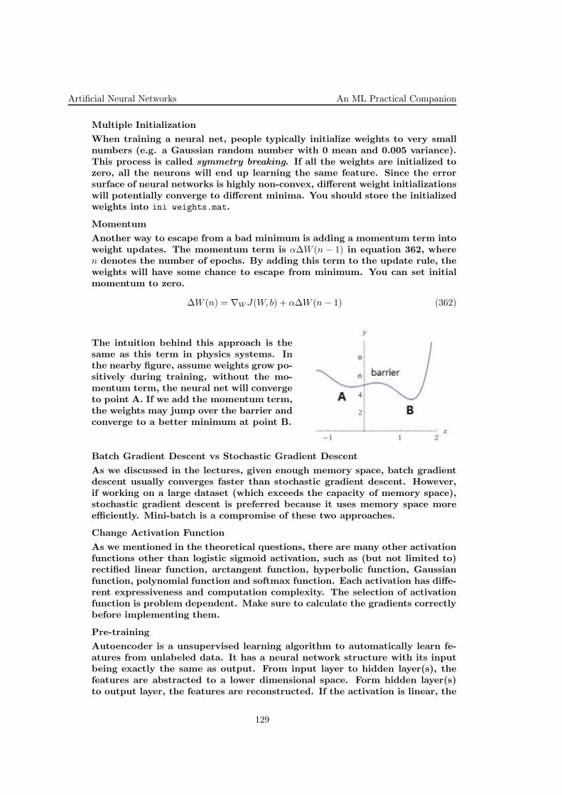
Artificial Neural Networks An ML Practical Companion
Multiple Initialization
When training a neural net, people typically initialize weights to very smallnumbers (e.g. a Gaussian random number with 0 mean and 0.005 variance).This process is called symmetry breaking. If all the weights are initialized tozero, all the neurons will end up learning the same feature. Since the errorsurface of neural networks is highly non-convex, different weight initializationswill potentially converge to different minima. You should store the initializedweights into ini weights.mat.
Momentum
Another way to escape from a bad minimum is adding a momentum term intoweight updates. The momentum term is α∆W (n − 1) in equation 362, wheren denotes the number of epochs. By adding this term to the update rule, theweights will have some chance to escape from minimum. You can set initialmomentum to zero.
∆W (n) = ∇WJ(W, b) + α∆W (n− 1) (362)
The intuition behind this approach is thesame as this term in physics systems. Inthe nearby figure, assume weights grow po-sitively during training, without the mo-mentum term, the neural net will convergeto point A. If we add the momentum term,the weights may jump over the barrier andconverge to a better minimum at point B.
Batch Gradient Descent vs Stochastic Gradient Descent
As we discussed in the lectures, given enough memory space, batch gradientdescent usually converges faster than stochastic gradient descent. However,if working on a large dataset (which exceeds the capacity of memory space),stochastic gradient descent is preferred because it uses memory space moreefficiently. Mini-batch is a compromise of these two approaches.
Change Activation Function
As we mentioned in the theoretical questions, there are many other activationfunctions other than logistic sigmoid activation, such as (but not limited to)rectified linear function, arctangent function, hyperbolic function, Gaussianfunction, polynomial function and softmax function. Each activation has diffe-rent expressiveness and computation complexity. The selection of activationfunction is problem dependent. Make sure to calculate the gradients correctlybefore implementing them.
Pre-training
Autoencoder is a unsupervised learning algorithm to automatically learn fe-atures from unlabeled data. It has a neural network structure with its inputbeing exactly the same as output. From input layer to hidden layer(s), thefeatures are abstracted to a lower dimensional space. Form hidden layer(s)to output layer, the features are reconstructed. If the activation is linear, the
129

An ML Practical Companion Artificial Neural Networks
network performs very similar to Principle Component Analysis (PCA). Aftertraining an autoencoder, you should keep the weights from input layer andhidden layers, and build a classifier on top of hidden layer(s). For implementa-tion details, please refer to Andrew Ng’s cs294A course handout at Stanford:http://web.stanford.edu/class/cs294a/sparseAutoencoder_2011new.pdf
More Neurons vs Less Neurons
As mentioned above, we should use more complicated models for underfittingcases, and simpler models for overfitting cases. In terms of neural networks,more neurons mean higher complexity. You should pick the size of hiddenlayer based on training accuracy and validation accuracy.
More Layers?
Adding one or two hidden layers may be useful, since the model expressivenessgrows exponentially with extra hidden layers. You can apply the same backpropagation technique as training a single hidden layer network. However,if you use even more layers (e.g. 10 layers), you are definitely going to getextremely bad results. Any networks with more than one hidden layer iscalled a deep network. Large deep network encounters the “vanishing gradient”problem using the standard back propagation algorithm (except convolutionalneural nets). If you are not familiar with convolutional neural nets, or trainingstacks of Restricted Boltzmann Machines, you should stick with a few hiddenlayers.
Sparsity
Sparsity on weights (LASSO penalty) forces neurons to learn localized infor-mation. Sparsity on activations (KL-divergence penalty) forces neurons tolearn complicated features.
Other Techniques
All the tricks above can be applied to both shallow networks and deep ne-tworks. If you are interested, there are other tricks which can be applied to(usually deep) neural networks:
• Dropout
• Model Averaging
[You can find these information in coursera lectures provided by GeoffreyHinton.]
130
Artificial Neural Networks An ML Practical Companion
54. (Perceptronul Rosenblatt:xxx calcul “mistake bounds”;xxx calcul margini; comparaţie cu SVM)
• MIT, 2006 fall, Tommy Jaakkola, HW1, pr. 1-2
Implement a Perceptron classifier in MATLAB. Start by implementing thefollowing functions:
− a function perceptron_train(X, y) where X and y are n × d and n × 1 ma-trices respectively. This function trains a Perceptron classifier on a trainingset of n examples, each of which is a d-dimensional vector. The labels for theexamples are in y and are 1 or −1. The function should return [theta, k], thefinal classification vector and the number of updates performed, respectively.You may assume that the input data provided to your function is linearlyseparable. Training the Perceptron should stop when it makes no errors atall on the training data.
− a function perceptron_test(theta, X_test, y_test) where theta is the clas-sification vector to be used. X_test and y_test are m × d and m × 1 matricesrespectively, corresponding to m test examples and their true labels. Thefunction should return test err, the fraction of test examples which weremisclassified.
For this problem, we have provided you two custom-created datasets. Thedimension d of both the datasets is 2, for ease of plotting and visualization.
a. Load data using the load p1 a script and train your Perceptron classifier onit. Using the function perceptron_test, ensure that your classifier makes noerrors on the training data. What is the angle between theta and the vector(1, 0)⊤? What is the number of updates ka required before the Perceptronalgorithm converges?
b. Repeat the above steps for data loaded from script load_p1_b. What isthe angle between theta and the vector (1, 0)⊤ now? What is the number ofupdates kb now?
c. For parts a and b, compute the geometric margins, γageom and γb
geom, of yourclassifiers with respect to their corresponding training datasets. Recall that
the distance of a point xt from the θ⊤x = 0 is |θ⊤xt
||θ|| |.
d. For parts a and b, compute Ra and Rb, respectively. Recall that for anydataset χ, R = max||x|||x ∈ χ.
e. Plot the data (as points in the X-Y plane) from part a, along with decisionboundary that your Perceptron classifier computed. Create another plot,this time using data from part b and the corresponding decision boundary.Your plots should clearly indicate the class of each point (e.g., by choosingdifferent colors or symbols to mark the points from the two classes). We havea provided a MATLAB function plot_points_and_classifier which you mayfind useful.
Implement an SVM classifier in MATLAB, arranged like the [above] Percep-tron algorithm, with functions svm_train(X, y) and svm_test(theta, X test,
y test). Again, include a printout of your code for these functions.
131

An ML Practical Companion Artificial Neural Networks
Hint : Use the built-in quadratic program solver quadprog(H, f, A, b) which
solves the quadratic program: min1
2x⊤Hx+f⊤x subject to the constraint Ax ≤
b.
f. Try the SVM on the two datasets from parts a and b. How different are thevalues of theta from values the Perceptron achieved? To do this comparison,should you compute the difference between two vectors or something else?
g. For the decision boundaries computed by SVM, compute the correspondinggeometric margins (as in part c). How do the margins achieved using the SVMcompare with those achieved by using the Perceptron?
132

Artificial Neural Networks An ML Practical Companion
55. (Kernelized perceptron)
• MIT, 2006 fall, Tommy Jaakkola, HW2, pr. 3
Most linear classifiers can be turned into a kernel form. We will focus hereon the simple perceptron algorithm and use the resulting kernel version toclassify data that are not linearly separable.
a. First we need to turn the perceptron algorithm into a form that involvesonly inner products between the feature vectors. We will focus on hyper-planes through origin in the feature space (any offset component [LC: is as-sumed to be] provided as part of the feature vectors). The mistake drivenparameter updates are: θ ← θ + ytφ(xt) if ytθ
⊤φ(xt) ≤ 0, where θ = 0 initially.Show that we can rewrite the perceptron updates in terms of simple additiveupdates on the discriminant function f(x) = θ⊤φ(x):
f(x)← f(x) + ytK(xt, x) if ytf(xt) ≤ 0,
where K(xt, x) = φ(xt)⊤φ(x) is any kernel function and f(x) = 0 initially.
b. We can replace K(xt, x) with any kernel function of our choice such asthe radial basis kernel where the corresponding feature mapping is infinitedimensional. Show that there always is a separating hyperplane if we use theradial basis kernel. hint : Use the answers to the previous exercise in thishomework (MIT, 2006 fall, Tommy Jaakkola, HW2, pr. 2).
c. With the radial basis kernel we can therefore conclude that the perceptronalgorithm will converge (stop updating) after a finite number of steps for anydataset with distinct points. The resulting function can therefore be writtenas
f(x) =
n∑
i=1
wiyiK(xi, x)
where wi is the number of times we made a mistake on example xi. Most ofwi’s are exactly zero so our function won’t be difficult to handle. The sameform holds for any kernel except that we can no longer tell whether the wi’sremain bounded (problem is separable with the chosen kernel). Implementthe new kernel perceptron algorithm in MATLAB using a radial basis andpolynomial kernels. The data and helpful scripts are provided in...
Define functionsalpha = train_kernel_perceptron(X, y, kernel_type) andf = discriminant_function(alpha, X, kernel_type, X_test)
to train the pereptron and to evaluate the resulting f(x) for test examples,respectively.
d. Load the data using the load_p3_a script. When you use a polynomialkernel to separate the classes, what degree polynomials do you need? Draw thedecision boundary (see the provided script plot_dec_boundary) for the lowest-degree polynomial kernel that separates the data. Repeat the process for theradial basis kernel. Briefly discuss your observations.
133
An ML Practical Companion Artificial Neural Networks
56. (Convolutional neural networks:xxx implementation and application on the MNIST dataset)
• CMU, 2016 fall, N. Balcan, M. Gormley, HW6xxx CMU, 2016 spring, W. Cohen, N. Balcan, HW7
In this assignment, we are going to implement a Convolution Neural Network(CNN) to classify hand written digits of MNIST921 data. Since the breakthro-ugh of CNNs on ImageNet classification (A. Krizhevsky, I. Sutskever, G. E.Hinton, 2012), CNNs have been widely applied and achieved the state the artof results in many areas of computer vision. The recent AI programs that canbeat humans in playing Atari game (V. Mnih, K. Kavukcuoglu et al, 2015)and Go (D. Silver, A. Huang et al, 2016) also used CNNs in their models.
We are going to implement the earliest CNN model, LeNet (Y. LeCun, L.Bottou, Y. Bengio, P. Haffner, 1998), that was successfully applied to classifyhand written digits. You will get familiar with the workflow needed to builda neural network model after this assignment.
The Stanford CNN course922 and UFLDL923 material are excellent for begin-ners to read. You are encouraged to read some of them before doing thisassignment.
A. We begin by introducing the basic structure and building blocks of CNNs.CNNs are made up of layers that have learnable parameters including weightsand bias. Each layer takes the output from previous layer, performs someoperations and produces an output. The final layer is typically a softmaxfunction which outputs the probability of the input being in different classes.We optimize an objective function over the parameters of all the layers andthen use stochastic gradient descent (SGD) to update the parameters to traina model.
Depending on the operation in the layers, we can divide the layers into fol-lowing types:
1. Inner product layer (fully connected layer)
As the name suggests, every output neuron of inner product layer has fullconnection to the input neurons. The output is the multiplication of theinput with a weight matrix plus a bias offset, i.e.:
f(x) = Wx+ b. (363)
This is simply a linear transformation of the input. The weight parameter Wand bias parameter b are learnable in this layer. The input x is d dimensionalcolumn vector, and W is a d× n matrix and b is n dimensional column vector.
2.Activation layer
We add nonlinear activation functions after the inner product layers to modelthe non-linearity of real data. Here are some of the popular choices for non-linear activation:
921http://yann.lecun.com/exdb/mnist/922http://cs231n.github.io/923http://ufldl.stanford.edu/tutorial/
134
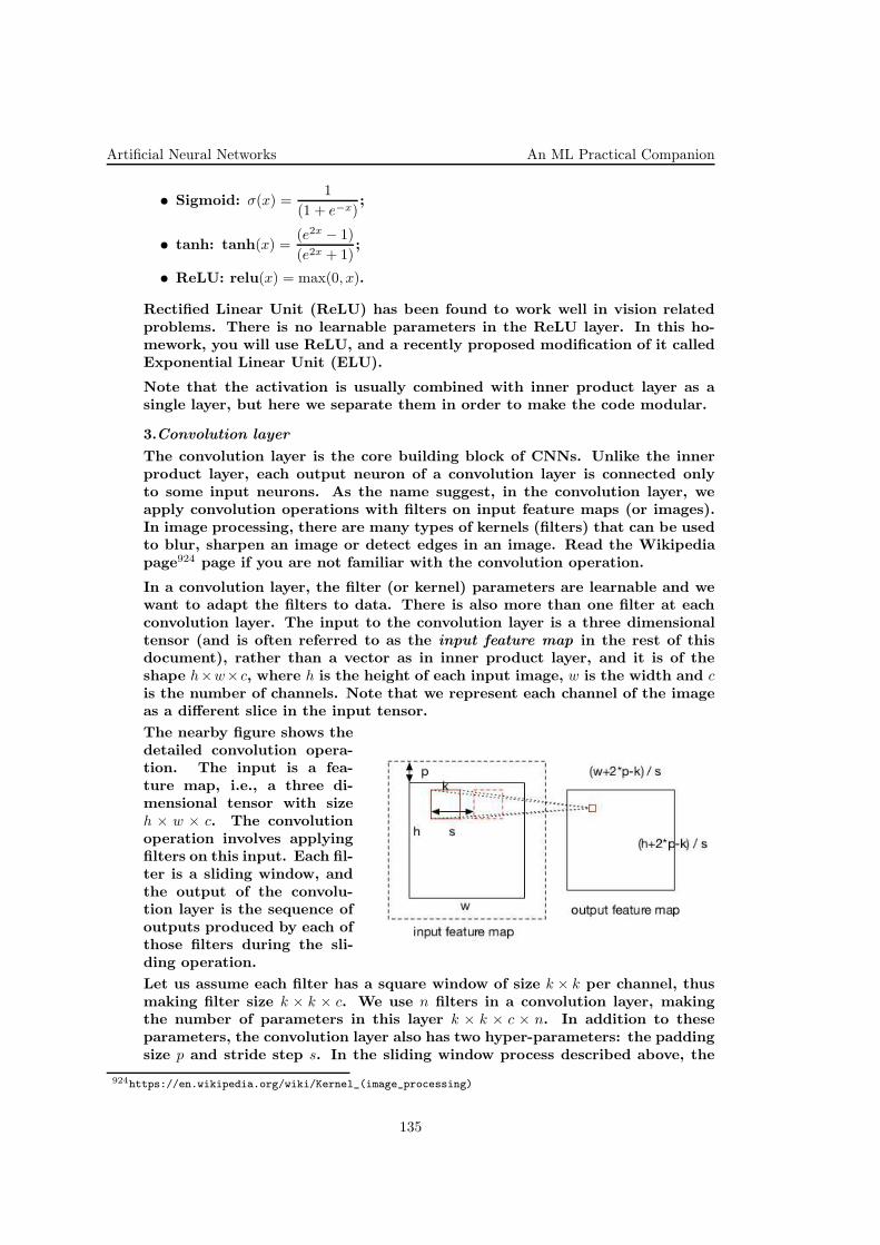
Artificial Neural Networks An ML Practical Companion
• Sigmoid: σ(x) =1
(1 + e−x);
• tanh: tanh(x) =(e2x − 1)
(e2x + 1);
• ReLU: relu(x) = max(0, x).
Rectified Linear Unit (ReLU) has been found to work well in vision relatedproblems. There is no learnable parameters in the ReLU layer. In this ho-mework, you will use ReLU, and a recently proposed modification of it calledExponential Linear Unit (ELU).
Note that the activation is usually combined with inner product layer as asingle layer, but here we separate them in order to make the code modular.
3.Convolution layer
The convolution layer is the core building block of CNNs. Unlike the innerproduct layer, each output neuron of a convolution layer is connected onlyto some input neurons. As the name suggest, in the convolution layer, weapply convolution operations with filters on input feature maps (or images).In image processing, there are many types of kernels (filters) that can be usedto blur, sharpen an image or detect edges in an image. Read the Wikipediapage924 page if you are not familiar with the convolution operation.
In a convolution layer, the filter (or kernel) parameters are learnable and wewant to adapt the filters to data. There is also more than one filter at eachconvolution layer. The input to the convolution layer is a three dimensionaltensor (and is often referred to as the input feature map in the rest of thisdocument), rather than a vector as in inner product layer, and it is of theshape h×w× c, where h is the height of each input image, w is the width and cis the number of channels. Note that we represent each channel of the imageas a different slice in the input tensor.
The nearby figure shows thedetailed convolution opera-tion. The input is a fea-ture map, i.e., a three di-mensional tensor with sizeh × w × c. The convolutionoperation involves applyingfilters on this input. Each fil-ter is a sliding window, andthe output of the convolu-tion layer is the sequence ofoutputs produced by each ofthose filters during the sli-ding operation.
Let us assume each filter has a square window of size k × k per channel, thusmaking filter size k × k × c. We use n filters in a convolution layer, makingthe number of parameters in this layer k × k × c × n. In addition to theseparameters, the convolution layer also has two hyper-parameters: the paddingsize p and stride step s. In the sliding window process described above, the
924https://en.wikipedia.org/wiki/Kernel_(image_processing)
135
An ML Practical Companion Artificial Neural Networks
output from each filter is a function of a neighborhood of input feature map.Since the edges have fewer neighbors, applying a filter directly is not feasible.To avoid this problem, inputs are typically padded (with zeros) on all sides,effectively making the the height and width of the padded input h + 2p andw + 2p respectively, where p is the size of padding. Stride (s) is the step sizeof convolution operation.
As the above figure shows, the red square on the left is a filter applied locallyon the input feature map. We multiply the filter weights (of size k×k×c) witha local region of the input feature map and then sum the product to get theoutput feature map. Hence, the first two dimensions of output feature map is[(h+ 2p− k)/s+ 1]× [(w + 2p− k)/s+ 1]. Since we have n filters in a convolutionlayer, the output feature map is of size [(h+2p−k)/s+1]× [(w+2p−k)/s+1]×n.
For more details about the convolutional layer, see Stanford’s course on CNNsfor visual recognition.925
4. Pooling layer
It is common to use pooling layers after convolutional layers to reduce the spa-tial size of feature maps. Pooling layers are also called down-sample layers,and perform an aggregation operation on the output of a convolution layer.Like the convolution layer, the pooling operation also acts locally on the fea-ture maps. A popular kind of pooling is max-pooling, and it simply involvescomputing the maximum value within each feature window. This allows usto extract more salient feature maps and reduce the number of parametersof CNNs to reduce over-fitting. Pooling is typically applied independentlywithin each channel of the input feature map.
5. Loss layer
For classification task, we use a softmax function to assign probability to eachclass given the input feature map:
p = softmax(Wx+ b). (364)
In training, we know the label given the input image, hence, we want tominimize the negative log probability of the given label:
l = − log(pj), (365)
where j is the label of the input. This is the objective function we would likeoptimize.
B. LeNet Having introduced the building components of CNNs, we now in-troduce the architecture of LeNet.
Layer Type ConfigurationInput size: 28× 28× 1Convolution k = 5, s = 1, p = 0, n = 20Pooling MAX, k = 2, s = 2, p = 0Convolution k = 5, s = 1, p = 0, n = 50Pooling MAX, k = 2, s = 2, p = 0IP n = 500ReLULoss
925http://cs231n.github.io/convolutional-networks/
136

Artificial Neural Networks An ML Practical Companion
The architecture of LeNet is shown in Table. 56. The name of the layer typeexplains itself. LeNet is composed of interleaving of convolution layers andpooling layers, followed by an inner product layer and finally a loss layer. Thisis the typical structure of CNNs.
137
An ML Practical Companion Clustering
7 Clustering
57. (Hierarchical clustering and K-means:xxx application on the yeast gene expression dataset)
• CMU, 2010 fall, Carlos Guestrin, HW4, pr. 3
Now that you have been in the Machine Learning class for almost 2 months,you have earned the first rank of number crunching machine learner. Recently,you landed a job at the Nexus lab of Cranberry Melon University. Your firsttask at the lab is to analyze gene expression data (which measures the levelsof genes in cells) for some mysterious yeast cells. You are given two datasets:a set of 12 yeast genes in yeast1.txt, and a set of 52 yeast genes in yeast2.txt.
You are told that these genes are critical to solve the “myster” of these cells.You just learnt clustering so you hope that this technique could help youpinpoint groups of genes that may explain the “mystery”. The format of thefiles is as follows: the first column lists an identifier for each gene, the secondcolumn lists a common name for the gene and a description of its functionand the remaining columns list expression values for the gene under variousconditions.
Your program should not use the gene descriptions when performing cluste-ring. However, it may be informative to see them in the output. These genesbelong to four categories for which the genes in each should exhibit fairlysimilar expression profiles.
a. Implement the agglomerative hierarchical clustering that you learnt inclass. You cannot use Matlab’s linkage function or any function that com-putes the linkage/tree. Use the Euclidean distance as the distance betweenexpression vectors of two genes. You only need to implement single linkageclustering.
Your output should be a tab-delimited text file. Each line of the file describesone internal node of the tree: the first column is the identifier of the first node,the second column is the identifier of the second node, and the third columnis the linkage between the two nodes. Note that each agglomeration occursat a greater distance between clusters than the previous agglomeration. Forleaf nodes, use the gene name as the identifier and for internal nodes, use theline number where the node was described.
To test your method, the output using single linkage on the small set is pro-vided in single1.txt:
YKL145W YGL048C 2.391171
YFL018C YGR183C 3.383814
YLR038C YLR395C 3.461156
3 2 4.144297
4 1 4.163976
YOR369C YPL090C 4.328152
5 YDL066W 4.463093
6 YOR182C 4.837613
7 YPR001W 5.246656
9 YGR270W 5.373565
10 8 6.050942
138

Clustering An ML Practical Companion
Submit the code and following output file single2.txt for single linkage clus-tering of the big set.
b. From the output tree, we can get K clusters by cutting the tree at a cer-tain threshold d. That is any internal nodes with the linkage greater thand are discarded. The genes are clustered according to the remaining nodes.Implement a function that output K clusters given the value K. Your func-tion should find the threshold d automatically from the constructed tree. Theoutput file lists the genes belong to each cluster. Each line of the file containstwo columns: the gene identifier (the first column in the original input file)and the description (the second column.) A blank line is used to separated theclusters. For the tree in single1.txt, to get 2 clusters, we use the threshold6.01 to cut the tree. The file 2single1.txt is an example output file as shownhere:
YPL090C RPS6A PROTEIN SYNTHESIS RIBOSOMAL PROTEIN S6A
YOR182C RPS30B PROTEIN SYNTHESIS RIBOSOMAL PROTEIN S30B
YOR369C RPS12 PROTEIN SYNTHESIS RIBOSOMAL PROTEIN S12
YPR001W CIT3 TCA CYCLE CITRATE SYNTHASE
YLR038C COX12 OXIDATIVE PHOSPHORYLATIO CYTOCHROME-C OXIDASE, SUBUNIT VIB
YGR270W YTA7 PROTEIN DEGRADATION 26S PROTEASOME SUBUNIT; ATPASE
YLR395C COX8 OXIDATIVE PHOSPHORYLATIO CYTOCHROME-C OXIDASE CHAIN VIII
YKL145W RPT1 PROTEIN DEGRADATION, UBI 26S PROTEASOME SUBUNIT
YGL048C RPT6 PROTEIN DEGRADATION 26S PROTEASOME REGULATORY SUBUNIT
YDL066W IDP1 TCA CYCLE ISOCITRATE DEHYDROGENASE (NADP+)
YFL018C LPD1 TCA CYCLE DIHYDROLIPOAMIDE DEHYDROGENASE
YGR183C QCR9 OXIDATIVE PHOSPHORYLATIO UBIQUINOL CYTOCHROME-C REDUCTASE SUBUNIT 9
Submit your code and the following tab-delimited output files: 2single2.txt,4single2.txt, 6single2.txt: 2, 4 and 6 clusters using single linkage on the bigdataset.
c. Describe another way to get K clusters from the constructed tree. Try tobe as succinct as possible. Implement your method. Submit the code and the3 output files: 2user2.txt, 4user2.txt, 6user2.txt. of running your method onthe big set to get 2, 4, 6 clusters respectively.
d. Implement K-means to cluster these genes. Make sure you use at least 10random initializations. Submit the code and the 3 output files: 2kmeans2.txt,4kmeans2.txt, 6kmeans2.txt of running K-means on the big set to get 2, 4, 6clusters respectively.
e. We can quantitatively compare the clustering as follows. For each clusterk, we can calculate the mean expression values of all genes which we call mk.The residual sum of squares (RSS) is defined as
∑
i
(xi −mci)⊤(xi −mci)
where xi is the gene expression of a gene i and ci is its cluster number.
For K = 2, 4, 6 clusters, report the RSS of the method in part b, your proposedmethod and K-means on the big dataset. Which method is better with respectto RSS?
139

An ML Practical Companion Clustering
f. Qualitatively compare the result of getting 6 clusters using the method inpart b, your proposed method with K-means on the big dataset. What do youobserve? Hint : The gene description may give you some clues on what thesegenes do in the cells.
Solution:
a. The code is available online in hcust.m and 2single.txt.
b. The code is available online in cuttree.m.
c. One way is to cut the K longest internal edges in the tree. The length ofthe internal edge = the increase in linkage when the cluster is combined inthe next step. This tells how far apart this cluster from the neighbor cluster.The code is available online in cuttree2.m.
d. The code is available online in kmean.m.
e. The code is available in calcRSS.m. The RSS is reported in the followingtable. K-means performs best in term of RSS.
RSSK-means CutTree CutTree
part b userK=2 839.2200 1.6288e+03 1.6583e+03K=4 638.7983 845.6614 1.6498e+03K=6 526.3841 854.7895 1.6455e+03
f. By looking at the gene annotation, which includes a short description ofthe gene function, we see that the method in part b provides clusters withmore coherent sets of genes.
140

Clustering An ML Practical Companion
58. (K-means: application to image compression)
• Stanford, 2012 spring, Andrew Ng, HW9
In this exercise, you will use K-means to compress an image by reducing thenumber of colors it contains. To begin, download ex9Data.zip and unpack itscontents into your Matlab/Octave working directory.
Photo credit: The bird photo used in this exercise belongs to Frank Woutersand is used with his permission.
Image Representation
The data pack for this exercise contains a 538-pixel by 538-pixel TIFF imagenamed bird_large.tiff. It looks like the picture below.
In a straightforward 24-bit color representation of this image, each pixel isrepresented as three 8-bit numbers (ranging from 0 to 255) that specify red,green and blue intensity values. Our bird photo contains thousands of colors,but we’d like to reduce that number to 16. By making this reduction, it wouldbe possible to represent the photo in a more efficient way by storing only theRGB values of the 16 colors present in the image.
In this exercise, you will use K-means to reduce the color count to K = 16.That is, you will compute 16 colors as the cluster centroids and replace eachpixel in the image with its nearest cluster centroid color.
141

An ML Practical Companion Clustering
Because computing cluster centroids on a 538 × 538image would be time-consuming on a desktop compu-ter, you will instead run K-means on the 128× 128 imagebird_small.tiff.
Once you have computed the cluster centroids on the small image, you willthen use the 16 colors to replace the pixels in the large image.
K-means in Matlab/Octave
In Matlab/Octave, load the small image into your program with the followingcommand:
A = double(imread(’bird_small.tiff’));
This creates a three-dimensional matrix A whose first two indices identifya pixel position and whose last index represents red, green, or blue. Forexample, A(50, 33, 3) gives you the blue intensity of the pixel at position y =50, x = 33. (The y-position is given first, but this does not matter so muchin our example because the x and y dimensions have the same size).
Your task is to compute 16 cluster centroids from this image, with each cen-troid being a vector of length three that holds a set of RGB values. Here isthe K-means algorithm as it applies to this problem:
K-means algorithm
1. For initialization, sample 16 colors randomly from the original small picture.These are your K means µ1, µ2, . . . , µK .2. Go through each pixel in the small image and calculate its nearest mean.
c(i) = argminj
∥
∥
∥x(i) − µj
∥
∥
∥
2
3. Update the values of the means based on the pixels assigned to them.
µj =
∑mi 1c(i)=jx
(i)
∑mi 1c(i) = j
4. Repeat steps 2 and 3 until convergence. This should take between 30 and100 iterations. You can either run the loop for a preset maximum number ofiterations, or you can decide to terminate the loop when the locations of themeans are no longer changing by a significant amount.
Note: In Step 3, you should update a mean only if there are pixels assigned toit. Otherwise, you will see a divide-by-zero error. For example, it’s possiblethat during initialization, two of the means will be initialized to the same color(i.e., black). Depending on your implementation, all of the pixels in the photothat are closest to that color may get assigned to one of the means, leavingthe other mean with no assigned pixels.
Reassigning colors to the large image
142

Clustering An ML Practical Companion
After K-means has converged, load the large image into your program andreplace each of its pixels with the nearest of the centroid colors you foundfrom the small image.
When you have recalculated the large image, you can display and save it inthe following way:imshow(uint8(round(large_image)))
imwrite(uint8(round(large_image)), ’bird_kmeans.tiff’);
When you are finished, compare your image to the one in the solutions.
Solution:
Here are the 16 colors appearing in the image:
© 2010-2012 Andrew Ng, Stanford University. All rights reserved.
143
An ML Practical Companion Clustering
59. (K-means: how to select Kxxx and the initial centroids (the K-means++ algorithm);xxx the importance of scaling the data across different dimensions)
• CMU, 2012 fall, E. Xing, A. Singh, HW3, pr. 1
In K-means clustering, we are given points x1, . . . , xn ∈ Rd and an integer K > 1,
and our goal is to minimize the within-cluster sum of squares (also known asthe K-means objective)
J(C,L) =n∑
i=1
||xi − Cli ||2,
where C = (C1, . . . , CK) are the cluster centers (Cj ∈ Rd), and L = (l1, . . . , ln) are
the cluster assignments (li ∈ 1, . . . ,K).Finding the exact minimum of this function is computationally difficult. Themost common algorithm for finding an approximate solution is Lloyd’s algo-rithm, which takes as input the set of points and some initial cluster centersC, and proceeds as follows:
i. Keeping C fixed, find cluster assignments L to minimize J(C,L). This steponly involves finding nearest neighbors. Ties can be broken using arbitrary(but consistent) rules.
ii. Keeping L fixed, find C to minimize J(C,L). This is a simple step that onlyinvolves averaging points within a cluster.
iii. If any of the values in L changed from the previous iteration (or if this wasthe first iteration), repeat from step i.
iv. Return C and L.
The initial cluster centers C given as input to the algorithm are often pickedrandomly from x1, . . . , xn. In practice, we often repeat multiple runs of Lloyd’salgorithm with different initializations, and pick the best resulting clusteringin terms of the K-means objective. You’re about to see why.
a. Briefly explain why Lloyd’s algorithm is always guaranteed to converge(i.e., stop) in a finite number of steps.
b. Implement Lloyd’s algorithm. Run it until convergence 200 times, eachtime initializing using K cluster centers picked at random from the set x1, . . . , xn,with K = 5 clusters, on the 500 two dimensional data points in . . .. Plot ina single figure the original data (in gray), and all 200 × 5 cluster centers (inblack) given by each run of Lloyd’s algorithm. You can play around withthe plotting options such as point sizes so that the cluster centers are clearlyvisible. Also compute the minimum, mean, and standard deviation of thewithin-cluster sums of squares for the clusterings given by each of the 200runs.
b. K-means++ is an initialization algorithm for K-means proposed by DavidArthur and Sergei Vassilvitskii in 2007:
i. Pick the first cluster center C1 uniformly at random from the data x1, . . . , xn.In other words, we first pick an index i uniformly at random from 1, . . . , n,then set C1 = xi.
144
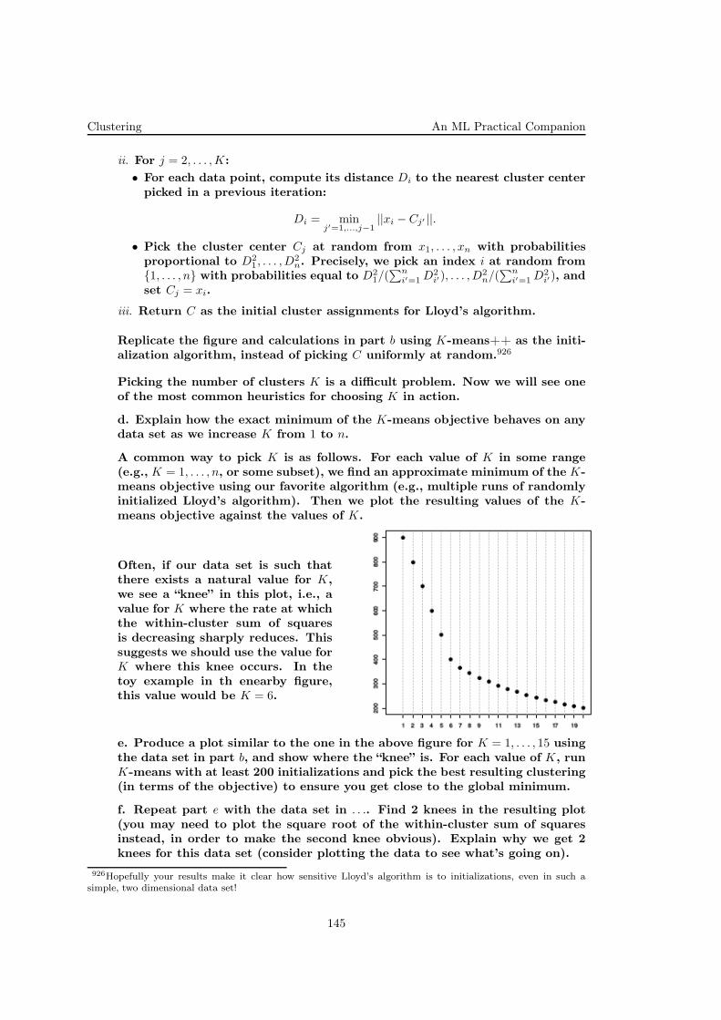
Clustering An ML Practical Companion
ii. For j = 2, . . . ,K:
• For each data point, compute its distance Di to the nearest cluster centerpicked in a previous iteration:
Di = minj′=1,...,j−1
||xi − Cj′ ||.
• Pick the cluster center Cj at random from x1, . . . , xn with probabilitiesproportional to D2
1, . . . , D2n. Precisely, we pick an index i at random from
1, . . . , n with probabilities equal to D21/(∑n
i′=1 D2i′), . . . , D
2n/(∑n
i′=1 D2i′), and
set Cj = xi.
iii. Return C as the initial cluster assignments for Lloyd’s algorithm.
Replicate the figure and calculations in part b using K-means++ as the initi-alization algorithm, instead of picking C uniformly at random.926
Picking the number of clusters K is a difficult problem. Now we will see oneof the most common heuristics for choosing K in action.
d. Explain how the exact minimum of the K-means objective behaves on anydata set as we increase K from 1 to n.
A common way to pick K is as follows. For each value of K in some range(e.g., K = 1, . . . , n, or some subset), we find an approximate minimum of the K-means objective using our favorite algorithm (e.g., multiple runs of randomlyinitialized Lloyd’s algorithm). Then we plot the resulting values of the K-means objective against the values of K.
Often, if our data set is such thatthere exists a natural value for K,we see a “knee” in this plot, i.e., avalue for K where the rate at whichthe within-cluster sum of squaresis decreasing sharply reduces. Thissuggests we should use the value forK where this knee occurs. In thetoy example in th enearby figure,this value would be K = 6.
e. Produce a plot similar to the one in the above figure for K = 1, . . . , 15 usingthe data set in part b, and show where the “knee” is. For each value of K, runK-means with at least 200 initializations and pick the best resulting clustering(in terms of the objective) to ensure you get close to the global minimum.
f. Repeat part e with the data set in . . .. Find 2 knees in the resulting plot(you may need to plot the square root of the within-cluster sum of squaresinstead, in order to make the second knee obvious). Explain why we get 2knees for this data set (consider plotting the data to see what’s going on).
926Hopefully your results make it clear how sensitive Lloyd’s algorithm is to initializations, even in such asimple, two dimensional data set!
145
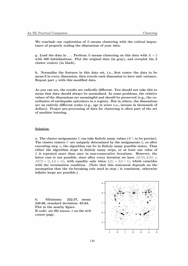
An ML Practical Companion Clustering
We conclude our exploration of K-means clustering with the critical impor-tance of properly scaling the dimensions of your data.
g. Load the data in . . .. Perform K-means clustering on this data with K = 2with 500 initializations. Plot the original data (in gray), and overplot the 2cluster centers (in black).
h. Normalize the features in this data set, i.e., first center the data to bemean 0 in every dimension, then rescale each dimension to have unit variance.Repeat part g with this modified data.
As you can see, the results are radically different. You should not take this tomean that data should always be normalized. In some problems, the relativevalues of the dimensions are meaningful and should be preserved (e.g., the co-ordinates of earthquake epicenters in a region). But in others, the dimensionsare on entirely different scales (e.g., age in years v.s., income in thousands ofdollars). Proper pre-processing of data for clustering is often part of the artof machine learning.
Solution:
a. The cluster assignments L can take finitely many values (Kn, to be precise).The cluster centers C are uniquely determined by the assignments L, so afterexecuting step ii, the algorithm can be in finitely many possible states. Thuseither the algorithm stops in finitely many steps, or at least one value ofL is repeated more than once in non-consecutive iterations. However, thelatter case is not possible, since after every iteration we have J(C(t), L(t)) ≥J(C(t + 1), L(t + 1)), with equality only when L(t) = L(t + 1), which coincideswith the termination condition. (Note that this statement depends on theassumption that the tie-breaking rule used in step i is consistent, otherwiseinfinite loops are possible.)
b. Minimum: 222.37, mean:249.66, standard deviation: 65.64.Plot in the nearby figure.R code: see file kmeans.r on the webcourse page.
146
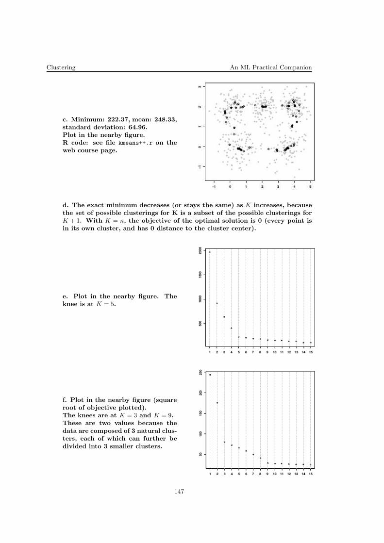
Clustering An ML Practical Companion
c. Minimum: 222.37, mean: 248.33,standard deviation: 64.96.Plot in the nearby figure.R code: see file kmeans++.r on theweb course page.
d. The exact minimum decreases (or stays the same) as K increases, becausethe set of possible clusterings for K is a subset of the possible clusterings forK + 1. With K = n, the objective of the optimal solution is 0 (every point isin its own cluster, and has 0 distance to the cluster center).
e. Plot in the nearby figure. Theknee is at K = 5.
f. Plot in the nearby figure (squareroot of objective plotted).The knees are at K = 3 and K = 9.These are two values because thedata are composed of 3 natural clus-ters, each of which can further bedivided into 3 smaller clusters.
147
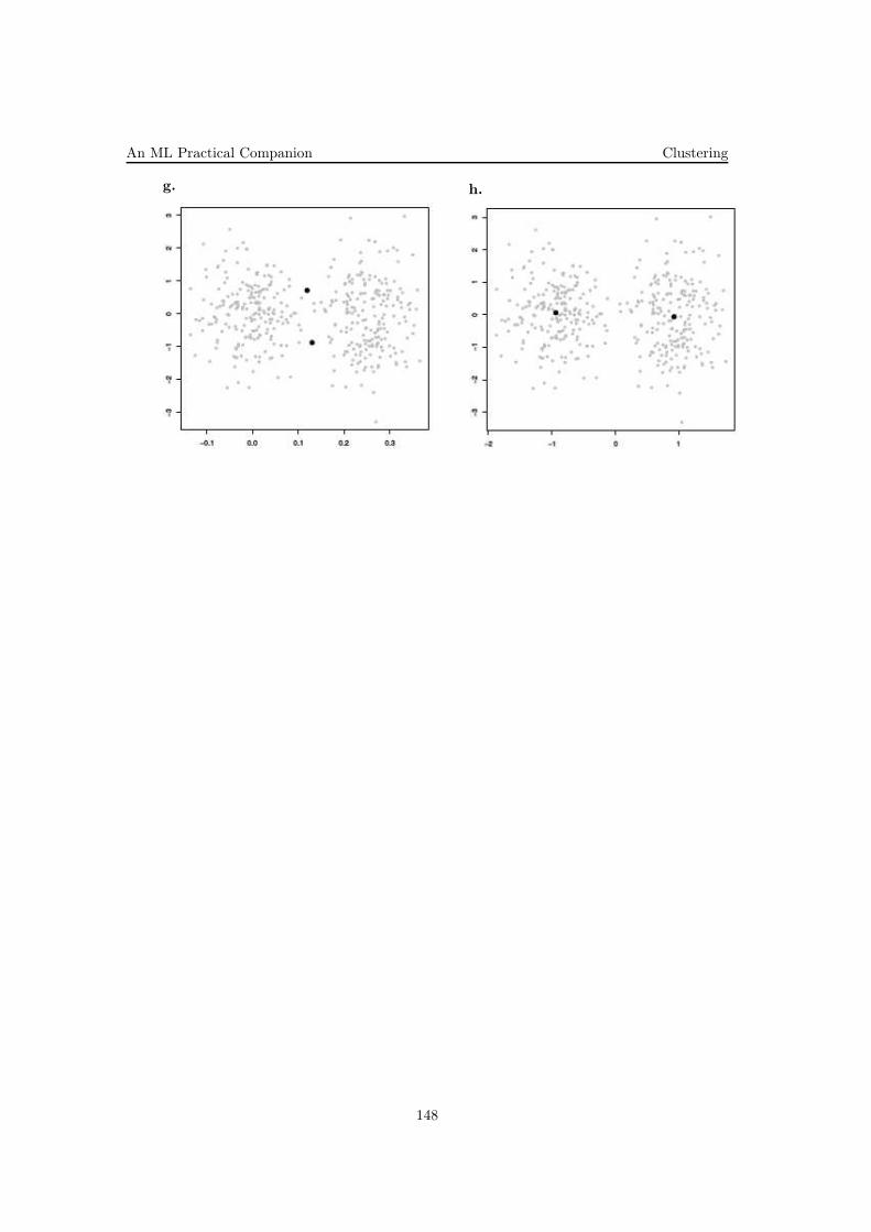
An ML Practical Companion Clustering
g. h.
148
Clustering An ML Practical Companion
60. (EM/GMM: implementation in Matlabxxx and application on data from R
1)
• · CMU, 2010 fall, Aarti Singh, HW4, pr. 2.3-5
a. Implement the EM/GMM algorithm using the update equations derivedin the exercise 43, the Clustering chapter in Ciortuz et al’s book).
b. Download the data set from . . .. Each row of this file is a training instancexi. Run your EM/GMM implementation on this data, using µ = [1, 2] andθ = [.33, .67] as your initial parameters. What are the final values of µ and θ?Plot a histogram of the data and your estimated mixture density P (X). Is themixture density an accurate model for the data?
To plot the density in Matlab, you can use:
density = @(x) (<class 1 prior> * normpdf(x, <class 1 mean>, 1)) + ...
(<class 2 prior> * normpdf(x, <class 2 mean>, 1));
fplot(density, [-5, 6]);
Recall from class that EM attempts to maximize the marginal data loglikelihoodℓ(µ, θ) =
∑n
i=1 logP (X = xi;µ, θ), but that EM can get stuck in local optima. In thispart, we will explore the shape of the loglikelihood function and determine if localoptima are a problem. For the remainder of the problem, we will assume that bothclasses are equally likely, i.e., θy = 1
2for y = 0, 1. In this case, the data loglikelihood
ℓ only depends on the mean parameters µ.
c. Create a contour plot of the loglikelihood ℓ as a function of the two mean para-meters, µ. Vary the range of each µk from −1 to 4, evaluating the loglikelihood atintervals of .25. You can create a contour plot in Matlab using the contourf function.Print out your plot and include in with your solution.
Does the loglikelihood have multiple local optima? Is it possible for EM to find anon-globally optimal solution? Why or why not?
149
An ML Practical Companion Clustering
61. (K-means and EM/GMM:xxx comparison on data from R
2)
• · CMU, 2010 spring, E. Xing, T. Mitchell, A. Singh, HW3, pr. 3
Clustering means partitioning your data into “natural” groups, usually because yoususpect points in a cluster have something in common. The EM algorithm and K-means are two common algorithms (there are many others). This problem will haveyou implement these algorithms, and explore their limitations.
The datasets for you to use are available online, along with a Matlab script forloading them. [Ask me if you’re having any trouble with it.] You can use anylanguage for your implementations, but you may not use libraries which alreadyimplement these algorithms (you can, however, use fancy built-in mathematicalfunctions, like Matlab or Mathematica provide).
a. In K-means clustering, the goal is to pick your clusters such that you minimizethe sum, over all points x, of |x− cx|2, where cx is the mean of the cluster containingx. [This should remind you of least-squares line fitting.] K-means clustering is NP-hard, but in practice this algoritm, also called Lloyd’s algorithm, works extremelywell.
Implement Lloyd’s algorithm, and apply it to the datasets provided. Plot eachdataset, indicating for each point which cluster is was placed in. How well do youthink K-means did for each dataset? Explain, intuitively, what (if anything) wentbadly and why.
b. A disadvantage of K-means is that the clusters cannot overlap at all. TheExpectation-Maximization algorithm deals with this by only probabilistically assig-ning points to clusters.
The thing to understand about the EM algorithm is that it’s a special case of MLE;you have some data, you assume a parameterized form for the probability distri-bution (a mixture of Gaussians is, after all, an exotic parameterized probabilitydistribution), and then you pick the parameters to maximize the probability of yourdata. But the usual MLE approach, solving ∂P (X|θ)
∂θ= 0, isn’t tractable, so we use
the iterative EM algorithm to find θ. The EM algorithm is guaranteed to convergeto a local optimum (I’m resisting the temptation to make you prove this :) ).
Implement the EM algorithm, and apply it to the datasets provided. Assume thatthe data is a mixture of two Gaussians; you can assume equal mixing ratios. Whatparameters do you get for each dataset? Plot each dataset, indicating for each pointwhich cluster it was placed in.
c. Modeling dataset 2 as a mixture of gaussians is unrealistic, but the EM algorithmstill gives an answer. Is there anything “fishy” about your answers which suggestssomething is wrong?
We usually do the EM algorithm with mixed Gaussians, but you can use any dis-tributions; a Gaussian and a Laplacian, three exponentials, etc. Write down theformula for a parameterized probability density suitable for modeling “ring-shaped”clusters in 2D; don’t let the density be 0 anywhere. You don’t need to work out theEM calculations for this density, but you would if this came up in your research.
d. With high-dimensional data we cannot perform visual checks, and problems cango unnoticed if we assume nice round, filled clusters. Describe in words a clusteringalgorithm which works even for weirdly-shaped clusters with unknown mixing ration.However, you can assume that the clusters do not overlap at all, and that you havea LOT of training data. Discuss the weaknesses of your algorithm. Don’t work outthe details for this problem; just convince me that you know the basic idea andunderstand its limitations.
150
Clustering An ML Practical Companion
62. (EM for mixtures of multi-variate Gaussiansxxx with independent components (along axis):xxx application to handwritten digit recognition)
• CMU, 2012 spring, Ziv Bar-Joseph, HW4, pr. 3.2
In this problem we will be implementing Gaussian mixture models and workingwith the digits data set. The provided data set is a Matlab file consisting of 500010×10 pixel hand written digits between 0 and 9. Each digit is a greyscale imagerepresented as a 100 dimensional row vector (the images have been down sampledfrom the original 28×28 pixel images. The variable X is a 5000×100 matrix and thevector Y contains the true number for each image. Please submit your code andinclude in your write-up a copy of the plots that you generated for this problem.
a. Implement the Expectation-Maximization (EM) algorithm for the axis alignedGaussian mixture model. Recall that the axis aligned Gaussian mixture modeluses the Gaussian Naive Bayes assumption that, given the class, all features areconditionally independent Gaussians. The specific form of the model is given below:
Zi ∼ Categorical(p1, . . . , pK)
Xi|Zi = z ∼ N
µz1
...µzd
,
(σz1)
2 0 . . . 0
0 (σz2)
2...
.... . . 0
0 . . . 0 (σzd)
2
b. Run EM to fit a Gaussian mixture model with 16 Gaussians on the digits data.Plot each of the means using subplot(4, 4, i) to save paper.
c. Evaluating clustering performance is difficult. However, because we have infor-mation about the ground truth data, we can roughly assess clustering performance.One possible metric is to label each cluster with the majority label for that clusterusing the ground truth data. Then, for each point we predict the cluster label andmeasure the mean 0/1 loss. For the digits data set, report your loss for settingsk = 1, 10 and 16.
151

An ML Practical Companion Clustering
63. (EM for mixtures of multi-variate Gaussiansxxx application to stylus-written digit recognition)
• MIT, 2001 fall, Tommi Jaakkola, HW4, pr. 1
152

Clustering An ML Practical Companion
64. (Aplicarea algoritmului EM [LC: pentru GMM]xxx la clusterizare de documente,xxx folosind sistemul WEKA)
• Edingurgh, Chris Williams and Victor Lavrenkoxxx Introductory Applied Machine Learning course, 3 Nov. 2008
A. Description of the dataset
This assignment is based on the 20 Newsgroups Dataset.927 This dataset is a col-lection of approximately 20,000 newsgroup documents, partitioned (nearly) evenlyacross 20 different newsgroups, each corresponding to a different topic. Some ofthe newsgroups are very closely related to each other (e.g. comp.sys.ibm.pc.hardware,comp.sys.mac.hardware), while others are highly unrelated (e.g. misc.forsale, soc.religion.christian).
There are three versions of the 20 Newsgroups Dataset. In this assignment we willuse the bydate Matlab version in which documents are sorted by date into trai-ning (60%) and test (40%) sets, newsgroup-identifying headers are dropped andduplicates are removed. This collection comprises roughly 61,000 different words,which results in a bag-of-words representation with frequency counts. More specifi-cally, each document is represented by a 61,000 dimensional vector that contains thecounts for each of the 61,000 different words present in the respective document.
To save you time and to make the problem manageable with limited computationalresources, we preprocessed the original dataset. We will use documents from only 5out of the 20 newsgroups, which results in a 5-class problem. More specifically the 5classes correspond to the following newsgroups 1:alt.atheism, 2:comp.sys.ibm.pc.hardware,3:comp.sys.mac.hardware, 4:rec.sport.baseball and 5:rec.sport.hockey. However, note herethat classes 2-3 and 4-5 are rather closely related. Additionally, we computed themutual information of each word with the class attribute and selected the 520 wordsout of 61,000 that had highest mutual information. Therefore, our dataset is a N ×520 dimensional matrix, where N is the number of documents.
The resulting representation is much more compact and can be used directly toperform our experiments in WEKA. There is, however, a potential caveat: Thepreprocessed dataset has been prepared by a busy and heavily underpaid teachingassistant who might have been a bit careless when preparing the dataset. Youshould keep this in mind and be aware of anomalies in the data when answering thequestions below.
B. Clustering
We are interested in clustering the newsgroups documents using the EM algorithm.The most common measure to evaluate the resulting clusters is the log-likelihoodof the data. We will additionally use the Classes to Clusters evaluation whichis straightforward to perform in WEKA, and look at the percentage of correctlyclustered instances. Note here that the data likelihood computed during EM isa probability density (NOT a probability mass function) and therefore the log-likelihood can be greater than 0. Use the train_20news_clean_best_tfidf.arff datasetand the default seed (100) to train the clusterers.
a. First, train and evaluate an EM clusterer with 5 clusters (you need to change thenumClusters option) using the Classes to Clusters evaluation option. Report thelog-likelihood and write down the percentage of correctly clustered instances (PC),you will need it in question b. Look at the Classes to Clusters confusion matrix.Do the clusters correspond to classes? Which classes are more confused with eachother? Interpret your results. Keep the result buffer for the clusterer, you will needit in question c.
927http://people.csail.mit.edu/jrennie/20Newsgroups/
153

An ML Practical Companion Clustering
HINT: WEKA outputs the percentage of incorrectly classified instances.
b. Now, train and evaluate different EM clusterers using 3, 4, 6 and 7 clusters andthe Classes to Clusters evaluation option. Tabulate the PC as a function of thenumber of clusters, include the PC for 5 clusters from the previous question. Whatdo you notice? Why do you think we get higher PC for 3 clusters than for 4? Keepthe result buffers for all the clusterers, you will need them in question c.
c. Re-evaluate the five clusterers using the validation set val_20news_best_tfidf.arff.Tabulate the log-likelihood on the validation set as a function of the number ofclusters. If the dataset was unlabeled, how many clusters would you choose to modelit in light of your results? Is it safe to make this decision based on experiments withonly one random seed? Why?
HINT: To re-evaluate the models, first select the Supplied test set option and choosethe appropriate dataset. Then right-click on the model and select Re-evaluate modelon current test set.
d. Now consider the model with 5 clusters learned using EM. After EM converges,each cluster is described in terms of the mean and standard deviation for each ofthe 500 attributes computed from the documents assigned to the respective cluster.Since the attributes are the normalized tf-idf weights for each word in a document,the mean vectors learned by EM correspond to the tf-idf weights for each word ineach cluster.
For each of the 5 clusters, we selected the 20 attributes with the highest meanvalues. Open the file cluster_means.txt. The 20 attributes for each cluster are displayedcolumnwise together with their corresponding mean value. By looking at the wordswith the highest tf-idf weights per cluster, which column (cluster) would you assignto each class (newsgroup topic) and why? Which two clusters are closest to eachother? Imagine that we want to assign a new document to one of the clusters andthat the document contains only the words “pitching” and “hit”. Would this be aneasy task for the clusterer? What about a document that contains only the words“drive” and “mac”? Write down three examples of 2-word documents that would bedifficult test cases for the clusterer.
154
Clustering An ML Practical Companion
65. (EM for GMM: application onxxx the yeast gene expression dataset)
• CMU, 2004 fall, Carlos Guestrin, HW2, pr. 3
In this problem you will implement a Gaussian mixture model algorithm and willapply it to the problem of clustering gene expression data. Gene expression measuresthe levels of messenger RNA (mRNA) in the cell. The data you will be workingwith is from a model organism called yeast , and the measurements were taken tostudy the cell cycle system in that organism. The cell cycle system is one of themost important biological systems playing a major role in development and cancer.
All implementation should be done in Matlab. At the end of each sub-problem whereyou need to implement a new function we specify the prototype of the function.
The file alphaVals.txt contains 18 time points (every 7 minutes from 0 to 119)measuring the log expression ratios of 745 cycling genes. Each row in this filecorresponds to one of the genes. The file geneNames.txt contains the names of thesegenes. For some of the genes, we are missing some of their values due to problemswith the microarray technology (the tools used to measure gene expression). Thesecases are represented by values greater than 100.
a. Implement (in Matlab) an EM algorithm for learning a mixture of five (18-dimensional) Gaussians. It should learn means, covariance matrices and weights foreach of the Gaussian. You can assume, however, independence between the differentdata points [LC, correct: features/attributes], resulting in a diagonal covariancematrix. How can you deal with the missing data? Why is this correct?
Plot the centers identified for each of the five classes. Each center should be plottedas a time-series of 18 time points.
Here is the prototype of the Matlab function you need to implement:
function[mu; s;w] = emcluster(x; k; ploton);
where
− x is input data, where each row is an 18-dimensional sample. Values above 100represent missing values;
− k is the number of desired clusters;
− ploton is either 1 or 0. If 1, then before returning the function plots log-likelihoodof the data after each EM iteration (the function will have to store the log-likelihoodof the data after each iteration, and then plot these values as a function of iterationnumber at the end). If 0, the function does not plot anything;
− s is a k by 18 matrix, with each row being diagonal elements of the correspondingcovariance matrix;
− w is a column vector of size k, where w(i) is a weight for i-th cluster.
The function outputs mu, a matrix with k rows and 18 columns (each row is a centerof a cluster).
b. How many more parameters would you have had to assign if we remove theindependence assumption above? Explain.
c. Suggest and implement a method for determining the number of Gaussians (orclasses) that are the most appropriate for this data. Please confine the set of choicesto values in between 2 and 7. (Hint : The method can use an empirical evaluationof clustering results for each possible number of classes). Explain the method.
Here is the prototype of the Matlab function you need to implement:
155

An ML Practical Companion Clustering
function[k, mu, s, w] = clust(x);
where
− x is input data, where each row is an 18-dimensional sample. Once again valuesabove 100 represent missing values;
− k is the number of classes selected by the function;
− mu, s and w are defined as in part a.
d. Use the Gaussians determined in part c to perform hard clustering of your databy finding, for each gene i the Gaussian j that maximizes the likelihood: P (i|j). Usethe function printSelectedGenes.m to write the names of the genes in each of theclusters to a separate file.
Here is the prototype of the matlab function you need to implement:
function[c] = hardclust(x; k; mu; s;w);
where
− x is defined as before;
− k, mu, s, w are the output variables from the function written in part c and aretherefore defined there;
− c is a column vector of the same length as the number of rows in x. For each row,it should indicate the cluster the corresponding gene belongs to.
The function should also write out files as specified above. The filenames should be:clust1, clust2, . . . , clustk.
e. Use compSigClust.m to perform the statistical significance test (everything isalready implemented here, so just use the function). Hand in a printout with thetop three categories for each cluster (this is the output of compSigClust.m).
Solution:
a. We have put a student code online. The implementation is pretty clear in terms ofeach step of the GMM iteration. The plot of the log-likelihood should be increasing.The plots of the centers of each cluster should look like a sinusoid shape thoughwith different phases (starting at a different point in the time series).
b. The number of clusters times the number of covariances, which is
k((d− 1) + (d− 2) + . . .+ 1) =kd
2(d− 1),
where d = 18 in our case.
c. This is essentially a model selection question. You could use different modelselection ways to solve it: cross validation, train-test, minimum description length,BIC.
d. For each data point, assign the cluster that has the maximum probability for thispoint.
e. Just run the code we provided on the cluster files you got above.
156

The EM Algorithm An ML Practical Companion
8 The EM Algorithm
66. (An EM algorithm for a Mixture of vectors of Bernoulli distributions;xxx application to handwritten digit recognition)
• · CMU, 2015 fall, A. Smola, B. Poczos, HW2, pr. 2
157
An ML Practical Companion The EM Algorithm
67. (EM for combining Naive Bayes classification withxxx a mixture of vectors of Bernoulli distributions,xxx and using a penalty term;xxx application to handwritten digit recognition)
• U. Toronto, Radford Neal,xxx “Statistical Methods for Machine Learning and Data Mining” course,xxx 2014 spring, HW2
In this assignment, you will classify handwritten digits with mixture models fittedby maximum penalized likelihood using the EM algorithm.
The data you will use consists of 800 training images and 1000 test images of han-dwritten digits (from US zip codes). We derived these images from the well-knownMNIST dataset, by randomly selecting images from the total 60000 training casesprovided, reducing the resolution of the images from 28× 28 to 14× 14 by averaging2 × 2 blocks of pixel values, and then thresholding the pixel values to get binaryvalues. A data file with 800 lines each containing 196 pixel values (either 0 or 1)is provided on webpage associated to this book. Another file containing the labelsfor these 800 digits (0 to 9) is also provided. Similarly, there is a file with 1000 testimages, and another file with the labels for these 1000 test images. You should lookat the test labels only at the very end, to see how well the methods do.
In this assignment, you should try to classify these images of digits using a generativemodel, from which you can derive the probabilities of the 10 possible classes giventhe observed image of a digit. You should guess that the class for a test digit is theone with highest probability (i.e., we will use a loss function in which all errors areequally bad).
The generative model we will use estimates the class probabilities by their frequ-encies in the training set (which will be close to, but not exactly, uniform over the10 digits) and estimates the probability distributions of images within each class bymixture models with K components, with each component modeling the 196 pixelvalues as being independent. It will be convenient to combine all 10 of these mixturemodels into a single mixture model with 10K components, which model both thepixel values and the class label. The probabilities for class labels in the componentswill be fixed, however, so that K components give probability 1 to digit 0, K com-ponents give probability 1 to digit 1, K components give probability 1 to digit 2,etc.
The model for the distribution of the label, yi, and pixel values xi,1, . . . , xi,196, fordigit i is therefore as follows:
P (yi, xi) =
10K∑
k=1
πkqk,yi
196∏
j=1
θxi,j
k,j (1− θk,j)1−xi,j
The data items, (yi, xi), are assumed to be independent for different cases i. Theparameters of this model are the mixing proportions, π1, . . . , π10K , and the probabi-lities of pixels being 1 for each component, θk,j for k = 1, . . . , 10K and j = 1, . . . , 196.The probabilities of class labels for each component are fixed, as
qk,y =
1 if k ∈ Ky + 1, . . . ,Ky +K0 otherwise
for k = 1, . . . , 10K and y = 0, . . . , 9.
You should write an R function to try to find the parameter values that maximize thelog-likelihood from the training data plus a “penalty”. (Note that with this “penalty”higher values are better.) The EM algorithm can easily be adapted to find maximumpenalized likelihood estimates rather than maximum likelihood estimates – referring
158

The EM Algorithm An ML Practical Companion
to the general version of the algorithm, the E step remains the same, but the Mstep will now maximize EQ[log P (x, z|θ) +G(θ)], where G(θ) is the “penalty”.
The “penalty” to use is designed to avoid estimates for pixel probabilities that arezero or close to zero, which could cause problems when classifying test cases (forexample, zero pixel probabilities could result in a test case having zero probabilityfor every possible digit that it might be). The penalty to add to the log likelihoodshould be
G(θ) = α10K∑
k=1
196∑
j=1
[log(θk,j) + log(1− θk,j)].
Here, α controls the magnitude of the penalty. For this assignment, you should fixα to 0.05, though in a real application you would probably need to set it by somemethod such as cross-validation. The resulting formula for the update in the M stepis
θk,j =α+
∑n
i=1 ri,kxi,j
2α+∑n
i=1 ri,k
where ri,k is the probability that case i came from component k, estimated in the Estep. You should write a derivation of this formula from the general form of the EMalgorithm presented in the lecture slides (modified as above to include a penaltyterm).
Your function implementing the EM algorithm should take as arguments the ima-ges in the training set, the labels for these training cases, the number of mixturecomponents for each digit class (K), the penalty magnitude (α), and the number ofiterations of EM to do. It should return a list with the parameter estimates (π andθ) and responsibilities (r). You will need to start with some initial values for theresponsibilities (and then start with an M step). The responsibility of componentk for item i should be zero if component k has qk,yi = 0. Otherwise, you shouldrandomly set ri,k from the uniform distribution between 1 and 2 and then rescalethese values so that for each i, the sum over k of ri,k is one.
After each iteration, your EM function should print the value of the log-likelihoodand the value of the log likelihood plus the penalty function. The latter should nevergo down – if it does, you have a bug in your EM function. You should use enoughiterations that these values have almost stabilized by the last iteration.
You will also need to write an R function that takes the fitted parameter valuesfrom running EM and uses them to predict the class of a test image. This functionshould use Bayes’ Rule to find the probability that the image came from each of the10K mixture components, and then add up the probabilities for the K componentsassociated with each digit, to obtain the probabilities of the image being of eachdigit from 0 to 9. It should return these probabilities, which can then be used toguess what the digit is, by finding the digit with the highest probability.
You should first run your program EM and prediction functions for K = 1, whichshould produce the same results as the naive Bayes method would. (Note that EMshould converge immediately with K = 1.) You should then do ten runs with K = 5using different random number seeds, and see what the predictive accuracy is foreach run. Finally, for each test case, you should average the class probabilities ob-tained from each of the ten runs, and then use these averaged probabilities to classifythe test cases. You should compare the accuracy of these “ensemble” predictionswith the accuracy obtained using the individual runs that were averaged.
You should hand in your derivation of the update formula for θ above, a listing ofthe R functions you wrote for fitting by EM and predicting digit labels, the R scriptsyou used to apply these functions to the data provided, the output of these scripts,including the classification error rates on the test set you obtained (with K = 1,with K = 5 for each of ten initializations, and with the ensemble of ten fits withK = 5), and a discussion of the results. Your discussion should consider how naive
159

An ML Practical Companion The EM Algorithm
Bayes (K = 1) compares to using a mixture (with K = 5), and how the ensemblepredictions compare with predicting using a single run of EM, or using the best runof EM according to the log likelihood (with or without the penalty).
Solution:
LC: Vezi ca exista ’solutie’ (la U.Toronto) pentru elaborarea pasului M.
With K = 1, which is equivalent to a naive Bayes model, the classification error rateon test cases was 0.190.
With K = 5, 80 iterations of EM seemed sufficient for all ten random initializations.The resulting models had the following error rates on the test cases:
0.157 0.151 0.158 0.156 0.166 0.162 0.163 0.159 0.158 0.153
These are all better than the naive Bayes result, showing that using more than onemixture component for each digit is beneficial.
I used the “show_digit” function to display the theta parameters of the 50 mixturecomponents as pictures (for the run started with the last random seed). It is clearthat the five components for each digit have generally captured reasonable variationsin writing style, except perhaps for a few with small mixing proportion (given asthe number above the plot), such as the second “1” from the top.
160

The EM Algorithm An ML Practical Companion
Using the ensemble predictions (averaging probabilities of digits over the ten runsabove), the classification error rate on test cases was 0.139. This is substantiallybetter than the error rate from every one of the individual runs, showing the benefitsof using an ensemble when there is substantial random variation in the results.
Note that the individual run with highest log likelihood (and also highest log likeli-hood + penalty) was the sixth run, whose error rate of 0.162 was actually the thirdworst. So at least in this example, picking a single run based on log likelihood wouldcertainly not do better than using the ensemble.
161

An ML Practical Companion The EM Algorithm
68. (An EM algorithm for learning the parameter of multinomial distributions;xxx application to an epidemiological study)
• · University of Chicago, 2004 spring, Statistics, course,xxx Michael Eichler, HW3, pr. 2.cde
162
The EM Algorithm An ML Practical Companion
69. (EM for a mixture of two exponential distributions)
• · U. Toronto, Radford Neal,xxx “Statistical Computation” course,xxx 2000 fall, HW 4
Suppose that the time from when a machine is manufactured to when it fails isis exponentially distributed (a common, though simplistic, assumption). However,suppose that some machines have a manufacturing defect that causes them to bemore likely to fail early than machines that don’t have the defect.
Let the probability that a machine has the defect be p, the mean time to failure formachines without the defect be g, and the mean time to failure for machines withthe defect be d. The probability density for the time to failure will then be thefollowing mixture density:
p · 1
µd
· exp(
− x
µd
)
+ (1− p) · 1
µg
exp
(
− x
µg
)
Suppose that you have a number of independent observations of times to failurefor machines, and that you wish to nd maximum likelihood estimates for p, µg,and µd. Write a program to find these estimates using the EM algorithm, withthe unobserved variables being the indicators of whether or not each machine isdefective. Note that the model is not identifiable — swapping µd and µg whilereplacing p with 1− p has no effect on the density. This isn’t really a problem; youcan just interpret whichever mean is smaller as the mean for the defective machines.
You may write your program so that it simply runs for however many iterations youspecify (i.e., you don’t have to come up with a convergence test). However, yourprogram should have the option of printing the parameter estimates and the loglikelihood at each iteration, so that you can manually see whether it has converged.(This will also help debugging.)
You should test your program on two data sets (ass4a.data and ass4b), each with 1000observations, which are on the web page associated to this book. You can read thisdata with a command like
> x <- scan("ass4a.data")
For both data sets, run your algorithm for as long as you need to to be sure thatyou have obtained close to the correct maximum likelihood estimates. To be sure,we recommend that you run it for hundreds of iterations or more (this shouldn’ttake long in R). Discuss how rapidly the algorithm converges on the two data sets.You may find it useful to generate your own data sets, for which you know the trueparameters values, in order to debug your program. You could start with data setswhere µg and µd are very different.
You should hand in your derivation of the formulas neeed for the EM algorithm,your program, the output of your tests, and your discussion of the results.
163
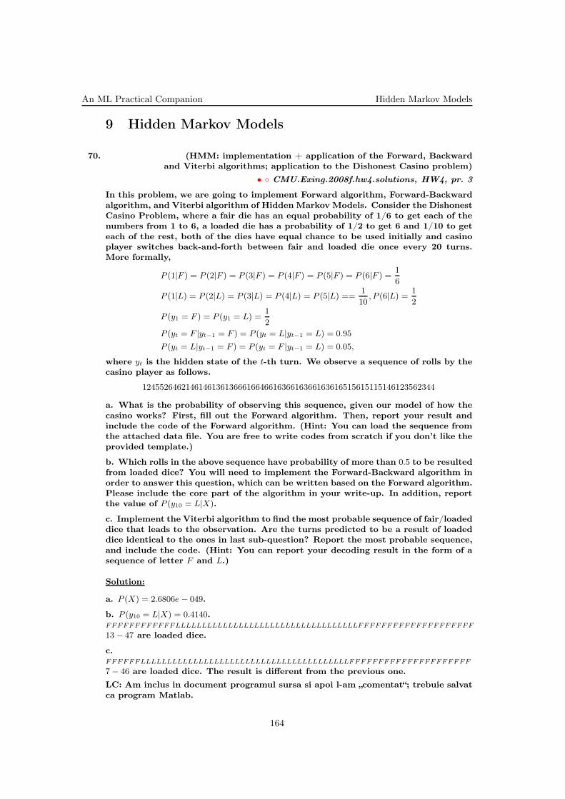
An ML Practical Companion Hidden Markov Models
9 Hidden Markov Models
70. (HMM: implementation + application of the Forward, Backwardxxx and Viterbi algorithms; application to the Dishonest Casino problem)
• CMU.Exing.2008f.hw4.solutions, HW4, pr. 3
In this problem, we are going to implement Forward algorithm, Forward-Backwardalgorithm, and Viterbi algorithm of Hidden Markov Models. Consider the DishonestCasino Problem, where a fair die has an equal probability of 1/6 to get each of thenumbers from 1 to 6, a loaded die has a probability of 1/2 to get 6 and 1/10 to geteach of the rest, both of the dies have equal chance to be used initially and casinoplayer switches back-and-forth between fair and loaded die once every 20 turns.More formally,
P (1|F ) = P (2|F ) = P (3|F ) = P (4|F ) = P (5|F ) = P (6|F ) =1
6
P (1|L) = P (2|L) = P (3|L) = P (4|L) = P (5|L) ==1
10, P (6|L) = 1
2
P (y1 = F ) = P (y1 = L) =1
2
P (yt = F |yt−1 = F ) = P (yt = L|yt−1 = L) = 0.95
P (yt = L|yt−1 = F ) = P (yt = F |yt−1 = L) = 0.05,
where yt is the hidden state of the t-th turn. We observe a sequence of rolls by thecasino player as follows.
1245526462146146136136661664661636616366163616515615115146123562344
a. What is the probability of observing this sequence, given our model of how thecasino works? First, fill out the Forward algorithm. Then, report your result andinclude the code of the Forward algorithm. (Hint: You can load the sequence fromthe attached data file. You are free to write codes from scratch if you don’t like theprovided template.)
b. Which rolls in the above sequence have probability of more than 0.5 to be resultedfrom loaded dice? You will need to implement the Forward-Backward algorithm inorder to answer this question, which can be written based on the Forward algorithm.Please include the core part of the algorithm in your write-up. In addition, reportthe value of P (y10 = L|X).
c. Implement the Viterbi algorithm to find the most probable sequence of fair/loadeddice that leads to the observation. Are the turns predicted to be a result of loadeddice identical to the ones in last sub-question? Report the most probable sequence,and include the code. (Hint: You can report your decoding result in the form of asequence of letter F and L.)
Solution:
a. P (X) = 2.6806e − 049.
b. P (y10 = L|X) = 0.4140.FFFFFFFFFFFFLLLLLLLLLLLLLLLLLLLLLLLLLLLLLLLLLLLFFFFFFFFFFFFFFFFFFFF
13− 47 are loaded dice.
c.FFFFFFLLLLLLLLLLLLLLLLLLLLLLLLLLLLLLLLLLLLLLLLFFFFFFFFFFFFFFFFFFFFF
7− 46 are loaded dice. The result is different from the previous one.
LC: Am inclus in document programul sursa si apoi l-am „comentat“; trebuie salvatca program Matlab.
164

Hidden Markov Models An ML Practical Companion
71. (Visible Markov Models and Hidden Markov Models:xxx application to language identification [in multilingual documents])
• MIT, 2001 fall, Tommi Jaakkola, HW4, pr. 2
In this problem, we will use Markov and Hidden Markov models to identify thelanguage of written sentences. For simplicity our representation of text will includeonly 27 symbols – the 26 letters of the Latin alphabet, and the space symbol. Anyaccented letter is represented as a non-accented letter, none-Latin letters are conver-ted to their closest Latin letters, and punctuation is removed. This representationnaturally looses quite a bit of information compared to the original ASCII text.This ’handicap’ is in part intentional so that the classification task would be a bitmore challenging. Most of the MATLAB code you will need here will be given. Youwill find the following routines useful (here and perhaps in some of your projects aswell):
readlines.m Reads a named text file, returning a cell array of the lines in the file.To get line i of cell-array lines returned from, e.g., lines = readlines(’cnn.eng’), uselinesi.
text2stream.m Converts a string (a line of text) into a row vector of numbers in therange 1, . . . , 27, according to the representation discussed above. So, for exam-ple, numberline = text2stream(lines1) would convert the first line of text from linesinto a row vector of numbers. The conversion of the full output of readlineswould have to be done line by line.
count.m Given text in a row vector representation and a width k, the function com-putes the count of all k-grams in the array. In other words, the function returnsa k-dimensional array representing the number of times each configuration of ksuccessive letters occurs in the text.
totalcount.m This function allows you to compute the accumulated counts from eachof the lines of text returned by readlines. Use this function to find the trainingcounts for the different languages.
A. Language identification using visible Markov models
Here we will construct a language classifier by using Markov models as class-conditionaldistributions. In other words, we will separately train a Markov model to representeach of the chosen languages: English, Spanish, Italian and German. The trainingdata is given in the files cnn.eng, cnn.spa, cnn.ita, cnn.ger, which contain several newsarticles (same articles in different languages), one article per line. We will first trya simple independent (zeroth-order Markov) model. Under this model, each suc-cessive symbol in text is chosen independently of other symbols. The language is inthis case identified based only on its letter frequencies.
a. Write a function naiveLL(stream,count1) which takes a 1-count (frequency of lettersreturned by count.m) and evaluates the log-likelihood of the text stream (row vectorof numbers) under the independent (zeroth-order Markov) model.
Extract the total 1-counts from the language training sets described above. Be-fore proceeding, let’s quickly check your function naiveLL. If you evaluate the log-likelihood of ’This is an example sentence’ using the English 1-counts from cnn.eng,you’ll get −76.5690, while the Spanish log-likelihood of the same sentence is −77.2706.
b. Write a short function naiveC which takes a stream, and several 1-counts corres-ponding to different languages, and finds the maximum-likelihood language for thestream. You could assume, e.g., that the 1-counts are stored in an array, where eachcolumn corresponds to a specific language. The format of the labels should be incorrespondence with the test_labels described below.
165

An ML Practical Companion Hidden Markov Models
c. The files song.eng, song.spa, song.ita, song.ger contain additional text in the fourlanguages. We will use these as the test set. For your convenience, we have providedyou with script generate test.m:
test_sentences = [ readlines(’song.eng’) ; ...readlines(’song.ger’) ; ...readlines(’song.spa’) ; ...readlines(’song.ita’) ] ;
test_labels = [ ones(17,1) ; ones(17,1)*2 ; ones(17,1)*3 ; ones(17,1)*4 ]
In order to study the performance of the classifier as a function of the length of teststrings, we will classify all prefixes of the lines in the test files. The provided routinetestC.m calculates the success probability of the classification, for each prefix length,over all the streams or strings in a given cell-array. You can call this function, e.g.,as follows
successprobs = testC(test_sentences,test_labels,’naiveC’,count1s);
where count1s provides the array of training counts that your function naiveC shouldaccept as an input.
Plot the success probability as a function of the length of the string. What is theapproximate number of symbols that we need to correctly assign new piece of textto one of the four languages?
d. In order to incorporate second order statistics, we will now move on to modelingthe languages with first-order Markov models.
Write a function markovLL(stream,count2) which returns the log-likelihood of astream under a first-order Markov model of the language with the specified 2-count.For the initial probabilities, you can use 1-counts calculated from the 2-counts.
Quick check : The English log-likelihood of ’This is an example sentence’ is −63.0643,while its Spanish log-likelihood is −65.4878. We are again assuming that you areusing the training sets described above to extract the 2-counts for the differentlanguages.
e. Write a corresponding function markovC.m that classifies a stream based on Markovmodels for various languages, specified by their 2-counts.
f. Try to classify the sentence ’Why is this an abnormal English sentence’. Whatis its likelihood under a Markov model for each of the languages? Which languagedoes it get classified as? Why does it not get classified as English?
g. Comment : When estimating discrete probability models, we often need to regularized theparameter estimates to avoid concluding that any configuration (e.g., two successive characters)have probability zero unless such the configuration appeared in the limited training set. Let θi,where
∑m
i=1 θi = 1, define a discrete probability distribution over m elements i ∈ 1, . . . ,m. Forthe purposes of estimation, we treat θi as parameters. Given now a training set summarized interms of the number of occurrences of each element i, i.e., ni, the maximum likelihood estimateof θi would be
θi =ni
∑m
j=1 nj
This is zero for all elements i that did not occur in the training set, i.e., when ni = 0. To avoidthis problem, we introduce a prior distribution over the parameters θi:
P (θ) =1
Z
m∏
i=1
θαii
166

Hidden Markov Models An ML Practical Companion
where Z is a normalization constant and αi ≥ 0’s are known as pseudo-counts. This prior, knownas a Dirichlet distribution, assigns the highest probability to
θi =αi
∑m
j=1 αj
Thus αi’s behave as if they were additional counts from some prior (imaginary) training set.We can combine the prior with the maximum likelihood criterion by maximizing instead thepenalized log-likelihood of the data (expressed here in terms of the training set counts ni):
J(θ) =
log-probability of data︷ ︸︸ ︷m∑
i=1
ni log(θi) +
log-prior︷ ︸︸ ︷
lnP (θ)
=m∑
i=1
ni ln(θi) +m∑
i=1
αi ln(θi) + constant
=m∑
i=1
(ni + αi) ln(θi) + constant
The maximizing θi is now
θi =ni + αi
∑m
j=1(nj + αj)
which will be non-zero whenever αi > 0 for all i = 1, . . . , m. Setting αi = 1/m would cor-respond to having a single prior observation distributed uniformly among the possible elementsi ∈ 1, . . . ,m. Setting αi = 1, on the other hand, would mean that we had m prior observations,observing each element i exactly once.
Add pseudocounts (one for each configuration) and reclassify the test sentence.What are the likelihoods now. Which language does the sentence get classified as?
h. Use testC.m to test the performance of Markov-based classification (with the cor-rected counts) on the test set. Plot the correct classification probability as a functionof the text length. Compare the classification performance to that of naiveC.m. (Turnin both plots).
B. Hidden Markov Models
We will now turn to a slightly more interesting problem of language segmentation:given a mixed-language text, we would like to identify the segments written indifferent languages. Consider the following simple approach: we will first find thecharacter statistics for each language by computing the 1-counts from the availabletraining sets as before. We will then go through the new text character by character,classifying each character to the most likely language (language whose independentmodel assigns the highest likelihood to the character). In other words, we woulduse naiveC to classify each character in the new text. To incorporate higher-orderstatistics, we could train a Markov model for each language (as before), and againassign the characters in the text to the most likely language.
i. Why would we expect the resulting segmentation not to agree with the truesegmentation? What would the resulting segmentation look like? What is thecritical piece of information we are not using in this approach?
j. Comment : We would rather model the multi-lingual text with a hidden Markov model. Forsimplicity, we will focus on segmenting text written in only two languages.
Suggest how a hidden Markov model can solve the problem you identified above.Provide an annotated transition diagram (heavy lines for larger transition probabi-lities) and describe what the output probabilities should be capturing.
167

An ML Practical Companion Hidden Markov Models
k. Comment : For some setting of the parameters, this HMM probably degenerates to theindependent model. Make sure you understand when this happens.
Now, load the example text from the file segment.dat. The text, mixed German andSpanish, is given in the variable gerspa as numbers in the range 1 . . . 27 (as before).You can use the provided function stream2text.m to view the numbers as letters.
The routine [hmm,ll] = esthmm(data, hmm) uses EM to find the maximum likelihoodparameters of a hidden Markov model, for a given output sequence(s). As discussedearlier, the EM algorithm has to start its search with some parameter setting. Thehmm input argument to esthmm provides this initial parameter setting.
The routine hmm = newhmm(numstates, numout) creates random HMM parameters foran HMM with numstates hidden states, and numout output symbols. An optionalthird argument controls the “non-uniformity” of the parameters.
Note: The orientation of the matrices Po and Pt is different from those in recitation:Pt(i, j) = P (statet = j|statet−1 = i) and Po(i, a) = P (Ot = a|statet = i).
With two different initializations, you will probably find two different HMMs. It isa good idea to run the EM algorithm multiple times, starting from slightly differentinitial settings. Every such run can potentially lead to a different result. Make sureyou understand how you would choose among the alternative solutions.
Estimate a two-state hidden Markov model with two different types of initial settingsof the state transition probabilities. First, set the transition probabilities close touniform values. In the second approach, make the “self-transitions” quite a bit morelikely than the transitions to different states. Which initialization leads to a bettermodel?
l. Now try to segment gerspa into German and Spanish, using a two-state hiddenMarkov model. You can then use the routine viterbi(sequence,hmm) to examine themost likely (maximum a posteriori probability or MAP) state sequence. The correctsegmentation of gerspa is given in gerspa_lang.
Examine the difference between your segmentation and the correct one. Do theerrors make sense?
m. Use the provided routine hmmposteriors(sequence, hmm) to calculate the per charac-ter posterior probabilities over the states. These are the γt(i) probabilities describedin lectures (t gives the character position in text and i specifies the state). Plot theseprobabilities as a function of the character position in the text sequence and turnin the plot. You might want to re-scale the axis using axis[0 3000 0 1.1].
n. Find the sequence of maximum a posteriori probability states. That is, for eachtime point t, find the state i with the maximum a posteriori probability P (statet =i|observedseq). Compare this state sequence with the maximum a posteriori statesequence. Are they different?
o. Give an example of a hidden Markov model, with two hidden states and two ou-tput symbols, and a length two output sequence, such that the MAP state sequencediffers from the sequence of MAP states. Be sure to specify all the parameters ofthe HMM (these need not be the maximum likelihood parameters for this specificlength two output sequence).
p. In the above example, we assumed no knowledge about the languages. We wo-uld like to improve the segmentation by incorporating some additional informationabout the languages such as single-character statistics.
What parameters of the HMM still need to be estimated? Modify the routineesthmm.m accordingly.
168

Hidden Markov Models An ML Practical Companion
q. (Optional) Use the single-character statistics you calculated from cnn.spa andcnn.ger to segment the text. What is the maximum likelihood estimate of the remai-ning parameters? Compare the resulting most likely state sequence to the one youfound without this prior information. Are they different?
r. Hidden Markov models can also be useful for classification. Suggest how youwould use HMMs in place of the Markov models described above to identify thelanguage of any specific (single-language) document. Specifically, list the routineswe have provided that you could make use of and describe which additional routinesyou would need.
s. (Optional) Use hidden Markov models, with a varying number of states, for thelanguage classification task investigated in the first part of this problem. Using thesame training set and test set as before, create a graph of the probability of correctclassification as a function of the length of the text. Discuss how the results compareto using naive classification and first-order Markov models, and how changing thenumber of hidden states affects the results.
Solution:
a.
function ll = naiveLL(stream,c1)lp = log(c1/sum(c1));
ll = sum(lp(stream));
b.
function [c,ll] = naiveC(stream,counts1)for i=1:size(counts1,2)
ll(i) = naiveLL(stream,counts1(:,i));end[dummy,c]=max(ll);
c. We carry out the following operations:
>> eng = readlines(’languages/cnn.eng’);>> ita = readlines(’languages/cnn.ita’);>> ger = readlines(’languages/cnn.ger’);>> spa = readlines(’languages/cnn.spa’);>> counts1 = [totalcount(eng,1), totalcount(ger,1), totalcount(spa,1), totalcount(ita,1)];>> p = testC(test_sentences, test_labels, ’naiveC’, counts1);>> plot(p)
169
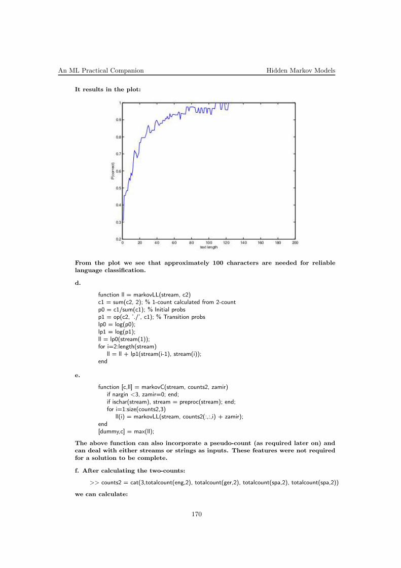
An ML Practical Companion Hidden Markov Models
It results in the plot:
From the plot we see that approximately 100 characters are needed for reliablelanguage classification.
d.
function ll = markovLL(stream, c2)c1 = sum(c2, 2); % 1-count calculated from 2-countp0 = c1/sum(c1); % Initial probsp1 = op(c2, ’./’, c1); % Transition probslp0 = log(p0);lp1 = log(p1);ll = lp0(stream(1));for i=2:length(stream)
ll = ll + lp1(stream(i-1), stream(i));end
e.
function [c,ll] = markovC(stream, counts2, zamir)if nargin <3, zamir=0; end;if ischar(stream), stream = preproc(stream); end;for i=1:size(counts2,3)
ll(i) = markovLL(stream, counts2(:,:,i) + zamir);end[dummy,c] = max(ll);
The above function can also incorporate a pseudo-count (as required later on) andcan deal with either streams or strings as inputs. These features were not requiredfor a solution to be complete.
f. After calculating the two-counts:
>> counts2 = cat(3,totalcount(eng,2), totalcount(ger,2), totalcount(spa,2), totalcount(spa,2))
we can calculate:
170
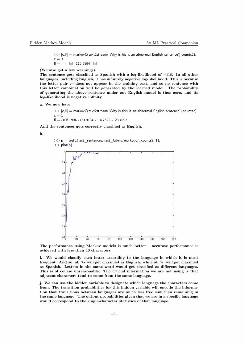
Hidden Markov Models An ML Practical Companion
>> [c,ll] = markovC(text2stream(’Why is his is an abnormal English sentence’),counts2);c = 3ll = -Inf -Inf -115.9894 -Inf
(We also get a few warnings).The sentence gets classified as Spanish with a log-likelihood of −116. In all otherlanguages, including English, it has infinitely negative log-likelihood. This is becausethe letter pair bn does not appear in the training text, and so no sentence withthis letter combination will be generated by the learned model. The probabilityof generating the above sentence under out English model is thus zero, and itslog-likelihood is negative infinity.
g. We now have:
>> [c,ll] = markovC(text2stream(’Why is this is an abnormal English sentence’),counts2);c = 1ll = -106.1994 -123.9184 -114.7622 -128.4992
And the sentences gets correctly classified as English.
h.
>> p = testC(test_sentences, test_labels,’markovC’, counts2, 1);>> plot(p)
The performance using Markov models is much better – accurate performance isachieved with less than 40 characters.
i. We would classify each letter according to the language in which it is mostfrequent. And so, all ’ts will get classified as English, while all ’a’ will get classifiedas Spanish. Letters in the same word would get classified as different languages.This is of course unreasonable. The crucial information we are not using is thatadjacent characters tend to come from the same language.
j. We can use the hidden variable to designate which language the characters comefrom. The transition probabilities for this hidden variable will encode the informa-tion that transitions between languages are much less frequent then remaining inthe same language. The output probabilities given that we are in a specific languagewould correspond to the single-character statistics of that language.
171
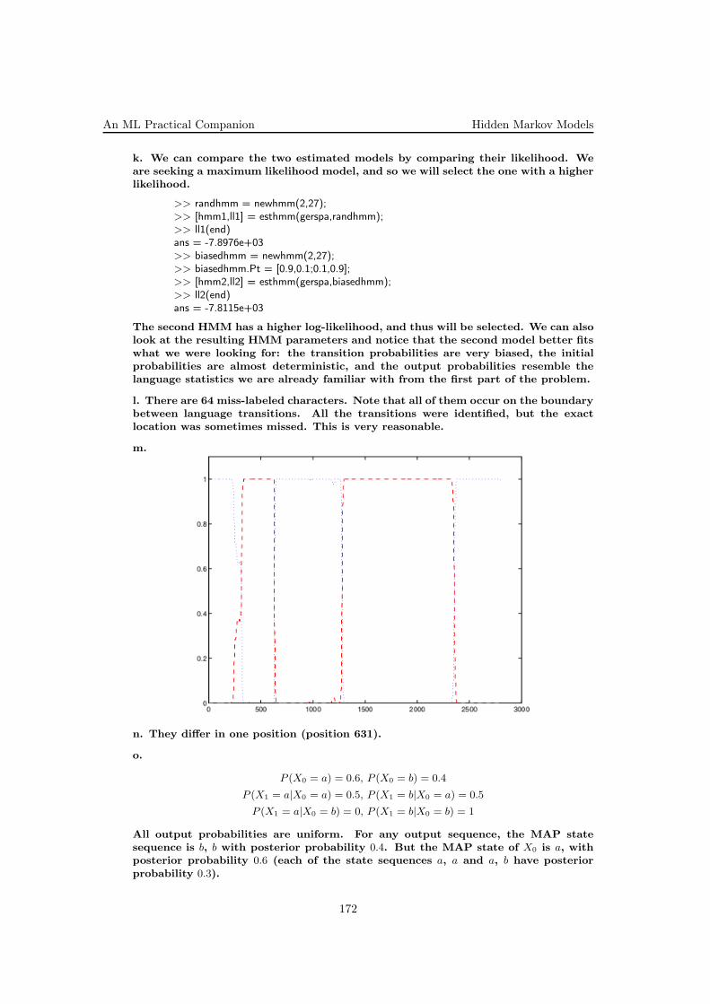
An ML Practical Companion Hidden Markov Models
k. We can compare the two estimated models by comparing their likelihood. Weare seeking a maximum likelihood model, and so we will select the one with a higherlikelihood.
>> randhmm = newhmm(2,27);>> [hmm1,ll1] = esthmm(gerspa,randhmm);>> ll1(end)ans = -7.8976e+03>> biasedhmm = newhmm(2,27);>> biasedhmm.Pt = [0.9,0.1;0.1,0.9];>> [hmm2,ll2] = esthmm(gerspa,biasedhmm);>> ll2(end)ans = -7.8115e+03
The second HMM has a higher log-likelihood, and thus will be selected. We can alsolook at the resulting HMM parameters and notice that the second model better fitswhat we were looking for: the transition probabilities are very biased, the initialprobabilities are almost deterministic, and the output probabilities resemble thelanguage statistics we are already familiar with from the first part of the problem.
l. There are 64 miss-labeled characters. Note that all of them occur on the boundarybetween language transitions. All the transitions were identified, but the exactlocation was sometimes missed. This is very reasonable.
m.
n. They differ in one position (position 631).
o.
P (X0 = a) = 0.6, P (X0 = b) = 0.4
P (X1 = a|X0 = a) = 0.5, P (X1 = b|X0 = a) = 0.5
P (X1 = a|X0 = b) = 0, P (X1 = b|X0 = b) = 1
All output probabilities are uniform. For any output sequence, the MAP statesequence is b, b with posterior probability 0.4. But the MAP state of X0 is a, withposterior probability 0.6 (each of the state sequences a, a and a, b have posteriorprobability 0.3).
172

Hidden Markov Models An ML Practical Companion
p. The output probabilities are now known and fixed. We only search for themaximum likelihood initial and transition probabilities. We make one change toesthmm.m: delete the following line:
hmm.Po = op(Nsx,’./’,sum(Nsx,2));
It would also be appropriate, though not necessary, to delete the calculation of Nsx,since it is now unused.
r. For each language, we would train a HMM (using esthmm.m) on the corpus oftexts for that languages. We would have to choose the number of hidden states ineach of those HMMs. We can set a fixed number of hidden states (e.g. any numberof hidden states above 27 would give us a model with a training accuracy at leastas good as a first order Markov model, but good training accuracy might not leadto good generalization). We can also use cross-validation to choose the number ofstates for each language model.
After training the models, in order to classify a sentence, we would compare thelikelihood of the query sentence under each of the models. This is given as thethird output parameter of hmmposteriors.m. However, all the other calculations inhmmposteriors.m are unnecessary (and take significant time) – it is enough to run onlythe forward calculation as follows:
function logPx = hmmloglikelihood(x,hmm)loga = logalpha(x,hmm);logPx = logsumexp(loga(:,n));
173
An ML Practical Companion Hidden Markov Models
72. (HMM for Protein Secondary Structure Analysis)
• CMU, 2011 spring, Roni Rosenfeld, HW9
A. Overview
Hidden Markov Models (HMMs) are powerful statistical models for modeling sequ-ential or time-series data, and have been successfully used in many tasks such asspeech recognition, protein/DNA sequence analysis, robot control, and informationextraction from text data. In this assignment, you will write much of the code res-ponsible for training/learning an HMM and apply the learned HMM to predict thesecondary structure of proteins.
This is mainly a programming assignment in C++, but in order to implement thealgorithm correctly, you need to understand many details of the underlying probabi-listic model. You need to understand the details of several algorithms, including theViterbi algorithm for finding the most likely transition path and the Baum-Welchalgorithm for parameter estimation. We will provide a great deal of “basic” code,so the expected knowledge of C++ is actually at the minimum. You will be askedto “fill in” the required code for three different tasks (algorithms):
(a) Compute the most likely path for an observed sequence of symbols from a givenHMM using the Viterbi algorithm.
(b) Estimate an HMM in a supervised way based on a sequence of symbols alongwith the observed state transitions.
(c) Train an HMM in an unsupervised way based on just a sequence of symbols.
You will also be asked to use your HMM program to predict the secondary structureof proteins. A common way of using an HMM is to train an HMM and then findthe most likely state transition path for a given sequence of observed symbols. Suchan optimal path can be interpreted as providing a sequence of tags correspondingto each of the symbols. The tags can also be interpreted as specifying a way ofsegmenting the observed sequence with a segment corresponding to a consecutivesequence of identical tags (i.e. states).
B. Prediction of Protein Secondary Structure
The problem of predicting protein structures is one of the many possible applicationsof HMM in the exciting emerging field of bioinformatics. One amazing fact in biologyis that the development and functions of any organism, whether it’s a human or avirus, are completely prescribed in deoxyribonucleic acid (DNA). However, little isknown about how such an encoding mechanism actually works; indeed, it is a majorchallenge in biology and bioinformatics to understand this mechanism.
Surprisingly, you do not really need to know much about biology in order to be ableto understand some of these challenges. Conceptually, DNA is a very long sequenceof four basic symbols A, T,G,C, each representing a different simple nucleic acidunit. It is known that three consecutive nucleic acid units would completely de-termine an amino acid. There are totally 20 distinct amino acids, each is typicallyrepresented by a distinct letter. The mapping from the 64 nucleic acid triples tothe 20 amino acids is fixed and completely known.
The building blocks of any organism are proteins. A protein is nothing but a sequ-ence of amino acids. One part (subsequence) of the whole DNA sequence woulddetermine a sequence of amino acids, i.e., one type of protein, while another woulddetermine another protein. There are usually many different kinds of proteins enco-ded in a long DNA sequence, but not all parts of a DNA sequence encode proteins– some are non-encoding regions. A protein can be represented as a sequence of
174
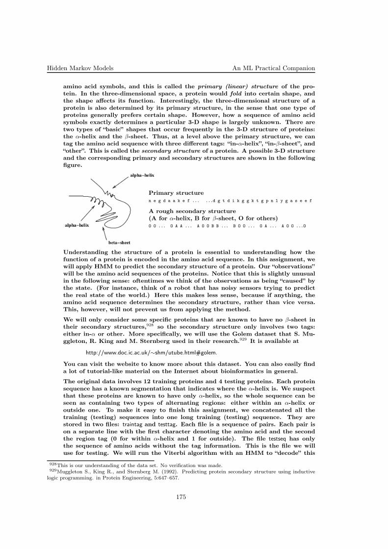
Hidden Markov Models An ML Practical Companion
amino acid symbols, and this is called the primary (linear) structure of the pro-tein. In the three-dimensional space, a protein would fold into certain shape, andthe shape affects its function. Interestingly, the three-dimensional structure of aprotein is also determined by its primary structure, in the sense that one type ofproteins generally prefers certain shape. However, how a sequence of amino acidsymbols exactly determines a particular 3-D shape is largely unknown. There aretwo types of “basic” shapes that occur frequently in the 3-D structure of proteins:the α-helix and the β-sheet. Thus, at a level above the primary structure, we cantag the amino acid sequence with three different tags: “in-α-helix”, “in-β-sheet”, and“other”. This is called the secondary structure of a protein. A possible 3-D structureand the corresponding primary and secondary structures are shown in the followingfigure.
Primary structuren e g d a a k e f ... ...d g t d i k g g k t g p n l y g a s e e f
A rough secondary structure(A for α-helix, B for β-sheet, O for others)O O ... O A A ... A O O B B ... B O O ... O A ... A O O ...O
Understanding the structure of a protein is essential to understanding how thefunction of a protein is encoded in the amino acid sequence. In this assignment, wewill apply HMM to predict the secondary structure of a protein. Our “observations”will be the amino acid sequences of the proteins. Notice that this is slightly unusualin the following sense: oftentimes we think of the observations as being “caused” bythe state. (For instance, think of a robot that has noisy sensors trying to predictthe real state of the world.) Here this makes less sense, because if anything, theamino acid sequence determines the secondary structure, rather than vice versa.This, however, will not prevent us from applying the method.
We will only consider some specific proteins that are known to have no β-sheet intheir secondary structures,928 so the secondary structure only involves two tags:either in-α or other. More specifically, we will use the Golem dataset that S. Mu-ggleton, R. King and M. Sternberg used in their research.929 It is available at
http://www.doc.ic.ac.uk/∼shm/utube.html#golem.
You can visit the website to know more about this dataset. You can also easily finda lot of tutorial-like material on the Internet about bioinformatics in general.
The original data involves 12 training proteins and 4 testing proteins. Each proteinsequence has a known segmentation that indicates where the α-helix is. We suspectthat these proteins are known to have only α-helix, so the whole sequence can beseen as containing two types of alternating regions: either within an α-helix oroutside one. To make it easy to finish this assignment, we concatenated all thetraining (testing) sequences into one long training (testing) sequence. They arestored in two files: traintag and testtag. Each file is a sequence of pairs. Each pair ison a separate line with the first character denoting the amino acid and the secondthe region tag (0 for within α-helix and 1 for outside). The file testseq has onlythe sequence of amino acids without the tag information. This is the file we willuse for testing. We will run the Viterbi algorithm with an HMM to “decode” this
928This is our understanding of the data set. No verification was made.929Muggleton S., King R., and Sternberg M. (1992). Predicting protein secondary structure using inductive
logic programming. in Protein Engineering, 5:647–657.
175
An ML Practical Companion Hidden Markov Models
sequence, i.e., to identify which part belongs to an α-helix and which does not. Thepredicted segmentation can be compared with the true tags in testtag to computethe prediction accuracy.
For this assignment, we will use the simplest measure of prediction accuracy, whichis defined as the percentage of tags that are correct. There is a Perl script in thedirectory (eval.pl) that will compute this accuracy for you. The usage is
% eval.pl testtag result
C. Summary of the HMM Algorithms
There are some excellent references on HMMs.930 Formally, we define an HMMas a 5-tuple (S, V,Π, A,B), where S = s0, s1, . . ., sN−1 is a finite set of N states,V = v0, v1, . . . , vM−1 is a set of M possible symbols in a vocabulary, Π = πi are theinitial state probabilities, A = aij are the state transition probabilities, B = bi(vk)are the output or emission probabilities. We use Λ = (Π, A,B) to denote all theparameters. The meaning of each parameter is as follows:
πi – the probability that the system starts at state i at the beginning
aij – the probability of going to state j from state i
bi(vk) – the probabillity of “generating” symbol vk at state i
Clearly, we have the following constraints
N−1∑
i=0
πi = 1
N−1∑
j=0
aij = 1 for i = 0, 1, 2, . . . , N − 1
M−1∑
k=0
bi(vk) = 1 for i = 0, 1, 2, . . . , N − 1
The three problems associated with an HMM are:
1. Evaluation: Evaluating the probability of an observed sequence of symbolsO = o1o2 . . . oT (oi ∈ V ), given a particular HMM, i.e., p(O|λ).
2. Decoding : Finding the most likely state transition path associated with anobserved sequence. Let q = q1q2 . . . qT be a sequence of states. We want to findq∗ = argmaxq p(q,O|λ), or equivalently, q∗ = argmaxq p(q|O, λ).
3. Training : Adjusting all the parameters λ to maximize the probability of gene-rating an observed sequence, i.e., to find λ∗ = argmaxΛ p(O|λ).
The first problem is solved by using the Forward iterative algorithms. The se-cond problem is solved by using the Viterbi algorithm, also an iterative algorithmto “grow” the best path by sequentially considering each observed symbol. Thelast problem is solved by the Baum-Welch algorithm (also known as the Forward-Backward algorithm), which uses the Forward and Backward probabilities to updatethe parameters iteratively. Below, we give the formulas for each of the step of thecomputation.
930For example, two classic references are L.R. Rabiner and B.H. Juang, An introduction to hidden
markov models, in IEEE ASSP Magazine, 1986. pp. 4–16, and Rabiner, L. R. (1989), A tutorial
on hidden Markov models and selected applications in speech recognition, in Proceedings of IEEE, 77(2), 257-286. Moreover, you can also find lots of online tutorials on HMM from the Internet, e.g.,http://www.cs.brown.edu/research/ai/dynamics/tutorial/Documents/HiddenMarkovModels.html and a Wikipediaentry, http://en.wikipedia.org/wiki/Hidden_Markov_model.
176

Hidden Markov Models An ML Practical Companion
The Forward Algorithm
Define αt(i) = p(o1, . . . , ot, qt = si|λ) as the probability that all the symbols up to timepoint t have been generated and the system is in state si at time t. The α’s can becomputed using the following recursive procedure:
1. α1(i) = πibi(o1) (Initially in state si and generating o1)2. For 1 . . . t < T, αt+1(i) = bi(ot+1)
∑N−1j=0 αt(j) aji (Generate ot+1, and we can arrive at
state si from any of the previous state sj with probability aji.)
Note that α1(i), . . . , αT (i) correspond to the T observed symbols.It is not hard to see that p(O|λ) =
∑N−1i=0 αT (i), since we may end at any of the N
states.
The Backward Algorithm
The α values computed using the forward algorithm are sufficient for solving thefirst problem, i.e., computing p(O|λ). However, in order to solve the third problem,we will need another set of probabilities – the β values.
Define βt(i) = p(ot+1, . . . , oT |qt = si, λ) as the probability of generating all the symbolsafter time t, given that the system is in state si at time t. Just like the α’s, the β’scan also be computed using the following backward recursive procedure:
1. βT (i) = 1 (We have no symbol to generate and we allow each state to be a possibleending state.)2. For 1 ≤ t < T , βt(i) =
∑j = 0N−1aij bj(ot+1) (Any state sj can be the state from
which ot+1 is generated.)
It is also easy to see that p(O|λ) = ∑N−1i=0 α1(i) β1(i); in fact, p(O|λ) = ∑
i = 0N−1αt(i) βt(i)for any t, 1 ≤ t ≤ T .
The Viterbi algorithm
The Viterbi algorithm is a dynamic programming algorithm that computes the mostlikely state transition path given an observed sequence of symbols. It is actuallyvery similar to the Forward algorithm, except that we will be taking a “max”, ratherthan a “
∑”, over all the possible ways to arrive at the current state under conside-
ration. However, the formal description of the algorithm inevitablely involves somecumbersome notations.
Let q = q1q2 . . . qT be a sequence of states. We want to find q∗ = argmaxq p(q|O, λ),which is the same as finding q∗ = argmaxq p(q,O|λ), since p(q,O|λ) = p(q|O, λ)p(O|λ) andp(O|λ) does not affect our choice of q.
The Viterbi algorithm “grows” the optimal path q∗ gradually while scanning each ofthe observed symbols. At time t, it will keep track of all the optimal paths endingat each of the N different states. At time t+ 1, it will then update these N optimalpaths.
Let q∗t be the optimal path for the subsequence of symbols O(t) = o1 . . . ot up to timet, and q∗t (i) be the most likely path ending at state si given the subsequence O(t).Let V Pt(i) = p(O(t), q∗t (i)|λ) be the probability of following path q∗t (i) and generatingO(t). Thus, q∗t = q∗t (k) where k = argmaxi V Pt(i) and q∗ = q∗T . The Viterbi algorithm isas follows:
1. V P1(i) = πi bi(o1) and q∗1(i) = (i).2. For 1 ≤ t < T , V Pt+1(i) = max0≤j<N V Pt(j) aji bi(ot+1) and q∗t (i) = q∗(k).(i),where k = argmax0≤j<N V Pt(j) aji bi (ot+1) and “.” is a concatenation operator of statesto form a path.
And, of course, q∗ = q∗T = q∗T (k), where k = argmax0≤i<N V PT (i).
177
An ML Practical Companion Hidden Markov Models
The The Baum-Welch Algorithm algorithm
Note that the last problem, i.e., finding λ∗ = argmaxλ p(O|λ), is precisely a maximumlikelihood estimation problem. If we can also observe the actual state transitionpath that has been followed to generate the symbols that we observed, then, theestimation would be extremely simple – We simply count the corresponding eventsand compute the relative frequency. However, the transition path is not observed.As a result, the maximum likelihood estimate, in general, can not be found analyti-cally. Fortunately, just like in the case of the mixture model of k Gaussians discussedin the class, we can also use an EM algorithm for HMM (called the Baum-Welch al-gorithm or Forward-Backward algorithm). Like in all other cases of applying an EMalgorithm, we will start with some random guess of the parameter values. At eachiteration, we compute the expected probability of all possible hidden state transitionpaths, and then re-estimate all the parameters based on the expected counts of thecorresponding events. The process is repeated until the likelihood converges.
The updating formulas can be expressed in terms of the α’s and β’s together with thecurrent parameter values. However, it is much easier to understand, if we introducetwo other notations. Define γt(i) = p(qt = si|O, λ) as the probability of being atstate si at time t given our observations, and ξt(i, j) = p(qt = si, qt+1 = sj |O, λ) asthe probability of going through a transition from state i to j at time t given theobservations. We have γt(i) =
∑N−1j=0 ξt(i, j), and also, for t = 1, . . . , T ,
γt(i) =αt(i) βt(i)
∑N−1j=0 αt(j) βt(j)
For t = 1, . . . , T − 1, ξt(i, j) is given by
ξt(i, j) =αt(i) aij bj(ot+1) βt+1(i)
∑N−1j=0 αt(j) βt(j)
=γt(i) aij bj(ot+1) βt+1(i)
βt(i)
The updating formulas for all the parameters are:
π′i = γ1(i)
a′ij =
∑T−1t=1 ξt(i, j)
∑N−1j=0
∑T−1t=1 ξt(i, j)
bi(vk)′ =
∑T
t=1,ot=vkγt(i)
∑T
t=1 γt(i)
D. Implementation of the HMM algorithms
The formulas given above can be implemented as they are, but the code would onlybe useful for a very short sequence. This is because many quantities would quicklyget extremely small as the sequence gets longer. There are generally two ways todeal with the problem: working on the logarithm domain or normalization. Takinglogarithm would convert the product of small quantities into a sum of logarithm ofthe quantities. This would easily work for the Viterbi algorithm. It can also be usedfor computing the α’s and β’s. Unfortunately, it is not helpful for computing theγ’s, since it would involve a sum of all the αt(i)’s, which would force us to get out ofthe logarithm domain. Below we present a normalization method that can neatlysolve the problem of underflow.
Our idea of normalization is to normalize αt(i) such that, αt(i), the normalized αt(i),would be proportional to αt(i) and sum to 1 over all possible states. That is,
N−1∑
i=0
αt(i) = 1
178

Hidden Markov Models An ML Practical Companion
and we want
αt(i) =t∏
k=1
ηk αt(i)
so,∏t
k=1 ηk =1
∑N−1i=0 αt(i)
=1
p(O(t)|λ) , and in particular,∏T
k=1 ηk =1
∑N−1i=0 αT (i)
=
1
p(O|λ) . Thus, αt(i) = p(qt = si|O(t), λ), compared with αt(i) = p(O(t), qt = si|λ).
The Normalized Forward Algorithm
The α’s can be computed in the same way as the α’s, only we do a normalization ateach step.
1. α1(i) = η1πibi(o1), where η1 =1
∑N−1k=0 πkbk(o1)
2. For 1 ≤ t < T , αt+1(i) = ηt+1bi(ot+1)∑N−1
j=0 α1(j)aji,
where ηt+1 =1
∑N−1k=0 bk(ot+1)
∑N−1j=0 αt(j)ajk
.
The Normalized Backward Algorithm
The β’s are normalized using the same normalizers as used for the α’s. That is, βt(i) =βt(i)
∏T
k=t+1 ηk, (and βT (i) = βT (i)), so that we see αt(i)βt(i) =∏T
k=1 ηk αt(i) βt(i) =
αt(i)βt(i)
p(O|λ) . Note that, unlike in the case of α’s, here, we are not requiring that the
β’s sum to one over all the states at any time point.
We can compute the β’s in exactly the same way as computing the β’s, only wewill normalize the β’s with the η’s which were already computed in the normalizedforward algorithm. That is,
1. βT (i) = βT (i) = 12. For 1 ≤ t < T, βt(i) = ηt+1
∑N−1i=0 βt+1(j) aij bj(ot+1).
The Updating Formulas Using Normalized α’s and β’s
We now give the updating formulas in terms of the normalized α’s and β’s.The γ’s can be computed in the same way, because the normalizers are cancelled.For t = 1, . . . , T ,
γt(i) =αt(i) βt(i)
∑N−1j=0 αt(j) βt(j)
For t = 1, . . . , T − 1, the ξ’s are computed with a slightly different formula:
ξt(i, j) =αt(i) aij bj(ot+1) ηt+1 βt+1(j)
∑N−1j=0 αt(j) βt(j)
=γt(i) aij bj(ot+1) ηt+1 βt+1(j)
βt(i)
Now that we can compute the γ’s and ξ’s using the normalized α’s and β’s, we canupdate the parameters using exactly the same updating formulas as we see in theprevious section. That is,
π′i = γ1(i)
a′ij =
∑T−1t=1 ξt(i, j)
∑N−1j=0
∑T−1t=1 ξt(i, j)
bi(vk)′ =
∑T
t=1,ot=vkγt(i)
∑T
t=1 γt(i)
You might have already noticed that the updating formulas generally involve theaccumulation of some expected counts (expressed in terms of γ’s and ξ’s) over all
179

An ML Practical Companion Hidden Markov Models
the possible time points t = 1, 2, . . . , T , and the expected counts at each time pointt depend only on the αt(i)’s, βt(i)’s, and ηt+1, in addition to the model parameters.Thus, in the most efficient implementation of Baum-Welch algorithm, such accu-mulation can be done at the same time of computing the β’s. In this assignment,however, we will implement the accumulation of counts as a separate pass.
E. The HMM Code Provided
We have provided a significant amount of code in C++ for this assignment. Thisincludes three files hmm.hpp, hmm.cpp, main.cpp and a makefile. The code and the ne-cessary sequence data are all in http://cs.cmu.edu/∼roni/10601-s11/assignments/hw9/basecode.tar.gz.The code is complete except that several key functions in hmm.cpp are not imple-mented. Your task is to implement them based on the algorithms specified in theprevious section.Important : You must implement the normalized version of the formulas as descri-bed in Section D. The program can be run in three different modes, depending onthe option given.
With option -d, it decodes a given sequence, i.e., computes the most likely path ofstate transitions given the sequence. The required input includes a model fileand a sequence file (without tags).
With option -c, it counts the relevant events in a given tagged sequence and savesthe model in the model file given. That is, it estimates the HMM parametersin a supervised way. The required input includes the number of states, a modelfile name and a tagged sequence file.
With option -t, it trains an HMM with a raw sequence without tags, and saves themodel in the model file given. That is, it estimates the HMM parameters in anunsupervised way. The required input includes the number of states, a modelfile name and a raw sequence file.
In any case, the program recognizes the following options:
• -m filename specifies a model file
• -s filename specifies a sequence file (tagged or untagged)
• -n integer specifies the desired number of states
You need to implement or complete the implementation of the following functionsin the file hmm.cpp.
1. void Decode(char *seqFile): This function should read in a sequence and computethe most likely state path using the Viterbi algorithm. It should print out a taggedsequence similar to testtag.2. void CountSequence(char *seqFile): This function should read in a tagged sequence fileand estimate all the HMM parameters based on the counting of the correspondingevents in the tagged sequence.3. void ComputeAlpha(int *seq, int seqLength): This function computes the normalized αvalues using the Forward algorithm. seq has the sequence of observed symbols, andis an array of length seqLength. It is 0-indexed, that is, the first observed symbol o1is in seq[0] and the last observed symbol oT is in seq[seqLength-1]. You can think ofseqLength as T in our formulas.4. void ComputeBeta(int *seq, int seqLength): This function computes the normalized βvalues using the Backward algorithm. seq is the same as in ComputeAlpha.5. void AccumulateCounts(int *seq, int seqLength): This function computes the γ’s and ξ’sand accumulates the counts for all the parameters. seq is the same as in ComputeAlpha.
The following is a brief explanation of how an HMM is represented in the providedcode. An HMM is represented by the class Model. We assume a fixed vocabulary
180
Hidden Markov Models An ML Practical Companion
that consists of all the 94 “readable/printable” ascii characters that are typically ona keyboard. More precisely, the symbol set is fixed as all the 94 ascii charactersfrom [33,!] to [126, ∼]. When a symbol is not observed in the data, its count isautomatically set to zero, effectively excluded from the model. The number of stateis stored in a variable N . The parameters of an N-state HMM are represented bythe following arrays:
1. Initial state probability (I)I is an array of length N (0-indexed), with I[s] representing the initial probabiltiyof being at state s.
2. State transition probability matrix (A)A is a 0-indexed two-dimensional array (N × N), with A[i][j] representing theprobability of going to state j from state i.
3. Output probability matrix (B)B is a 0-indexed two-dimensional array (M × N), with B[o][s] representing theprobability of generating output symbol o at state s. M is the number of uniquesymbols (currently 94, stored in SYMNUM). Note that the observed charactercan not be used directly as an index to access the entries of matrix B; it must benormalized by subtracting the “lowest” character baseChar defined in the classModel. For example, to find out the probability of generating ’C’ from state 1,use B[’C’-baseChar][1].
More specific instructions on how to implement them can be found in the embeddeddocumentation in the provided code. In all the cases, run gmake to recompile thecode after you change the code.
F. Finding the Most Likely State Path (Viterbi Algorithm)
a. Give an explanation of your HMM. Especially, how many states do you have?What do the states represent? What is the observation vocabulary? What parame-ters does your HMM have?
b. Complete the implementation of the Decode function. The function is mostlyimplemented except the part of Viterbi iteration for growing the most likely path.Fill in the appropriate code to make it work. The frame code provided in the Decodefunction is meant to minimize your work on implementing the Viterbi algorithm,but you should feel free to change any part of the provided code in the Decodefunction, including implementing the whole function on your own. Using logarithmto avoid underflow. Test your code using the two example model files and sequencefiles provided. That is, to run the following command:
% hmm -d -m samplemod1 -s sampleseq1 > sampletag1% hmm -d -m samplemod2 -s sampleseq2 > sampletag2
Your program should tag every “a” with “0” and every “b” with “1” for sampleseq1,and all the first eight symbols with “0” and the last eight symbols with “1” in thecase of sampleseq2.
c. If the results are as expected for these two examples, great! Continue to run thedecoding algorithm on the real protein sequence. Do the following:
% hmm -d -m mod.test -s testseq > result6c
“mod.test” is an HMM constructed based on the tags available on the testing sequ-ence. Evaluate the prediction accuracy with “eval.pl”. What is the accuracy? Thesegmentation accuracy should be above 0.7. If not, your implementation is probablyincorrect.
d. Take a look at the model specified in samplemod1 and samplemod2. Explain brieflywhy the program should tag the two sequences as it did. In particular explain briefly
181
An ML Practical Companion Hidden Markov Models
why it tagged the first b with “0” and the last a with “1” in sampleseq2 even thoughthe output probability distribution given state “0” strongly favors a and the outputprobability distribution given state “1” strongly favors b. Modify samplemod2 so that,when decoding sampleseq2, the program would tag all symbols with “0” except the lasttwo b’s which would be tagged as “1”. Name the modified model file as samplemod6d.
G. Supervised Training of HMM
a. Complete the implementation of the function CountSequence. This function ismostly implemented except the part of counting the relevant events for estimatingthe HMM parameters. Fill in the appropriate code so that it will count the followingwith the corresponding counters.
• How many times it starts with state s i (use ICounter)
• How many times a transition (from state si to sj) has happened (use ACounter)
• How many times character c is generated from state si (use BCounter)
For each of the three counters, change the counter as well as the correspondingnormalizer (i.e., INorm, ANorm, and BNorm). (These normalizers are to normalizethe counts in order to obtain probabilities. They have nothing to do with thenormalization discussed in Section D, which is to avoid underflow.) Take a look atthe function UpdateParameter(), if you are not sure how these counters and normalizersare used in the provided code.
Test your code using the tagged sequence (taggedsampleseq1) by running the followingcommand: (taggedsampleseq1 should be identical to the sampletag2 that you got.)
% hmm -c -n 2 -m samplesupmod7a -s taggedsampleseq1
Take a look at samplesupmod7a. If your implementation is correct, you should get amodel that would tend to generate “a” when at state “0” and tend to generate “b”when at state “1”.
b. Now train an HMM using the testing protein data and test the HMM on theraw testing sequence. That is, do the following
% hmm -c -n 2 -m mod7b.test -s testtag% hmm -d -m mod7b.test -s testseq > result7b1
Evaluate result7b1 with eval.pl. What is the prediction accuracy? It should be verysimilar to what you got in part F.b. Now train an HMM using the training proteindata and test the HMM on the raw testing sequence. That is, do the following
% hmm -c -n 2 -m mod7b.train -s traintag% hmm -d -m mod7b.train -s testseq > result7b2
Evaluate result7b2 with eval.pl. What is the prediction accuracy? It should be above0.55. If not, you may not have implemented the algorithm correctly. How is result7b2compared with result7b1? Which one has a better accuracy? Why?
c. Compare samplesupmod7a and samplemod2. Are they similar? Is this expected? Howare they different? Give an example of sequence for which samplesupmod7a would givea different decoding than samplemod2 (i.e., When running with option -d, you will getdifferent results). Name the sequence file sampleseq7c.
H. Unsupervised Training of HMM (Baum-Welch Algorithm)
a. In this part of the assignment, you are asked to complete the implementationof training an HMM with the Baum-Welch algorithm. The high level process, e.g.,the iterations, is already implemented in the function UpdateHMM. You will need to
182

Hidden Markov Models An ML Practical Companion
implement function ComputeAlpha, ComputeBeta, and complete function AccumulateCo-unts by inserting appropriate code for computing the Y ’s and ξ’s and the code foraccumulating the expected counts for the three groups of parameters according tothe formulas given in Section D.
There are more concrete instructions on how to implement each of the three func-tions within the code. You might find it useful (for debugging) to uncomment thefunction call to print out the α’s and the β’s in the function UpdateHMM.
b. Test your implementation by training on sampleseq2
% hmm -t -n 2 -m sampleunsupmod8b -s sampleseq2
Take a look at sampleunsupmod8b. Does the learned model capture some of the pat-terns in sampleseq2? Repeat the command above 20 times. Do you get the samemodel in sampleunsupmod8b and the same likelihood every time? Explain why youmight get a different model with a different likelihood sometimes.
Now choose a model with the highest likelihood from the 20 runs, and compare thecorresponding sampleunsupmod8b with samplemod2. Are they similar? Remember thatsince we are doing unsupervised training, state “0” and “1” may switch their roles.Now, use this sampleunsupmod8b to decode sampleseq2, i.e., do,
% hmm -d -m sampleunsupmod8b -s sampleseq2 > result8b
What do you get? Did you get the same tagging as sampletag2, which is produced byusing samplemod2.
c. Now, train the HMM on the protein testing data (i.e., assuming no labelledtraining data).
% hmm -t -n 2 -m mod8c.test -s testseq% hmm -d -m mod8c.test -s testseq>result8c
Note that since this is unsupervised training, the two states (0 and 1) may pick uptheir roles fairly arbitrarily, i.e., either state 0 or state 1 can mean within an α-helix.So, you need to evaluate the results in two different ways: assuming either 0 or 1to be within an α-helix. For such evaluation, we provided a different Perl scriptevalflip.pl. You should use evalflip.pl to evaluate result8c. The usage is exactly the sameas eval.pl.
Repeat this process at least 10 times. Do you get the same likelihood, the samemodel, and the same accuracy every time? Record and report the accuracy eachtime. What is the best of all the recorded accuracy numbers? How is this bestaccuracy compared with the accuracy of assigning the same tag to all the symbolsin testseq, which is 0.5216 when evaluated using evalflip.pl? How is this best accuracycompared with result7b1 and result7b2? Take a look at the segmentation provided bythis best model, and visually compare it with the true segmentation in testtag. Doesthe trained model seem to capture some of the true segment boundaries?
Note: This is a big programming assignment and can take more time than you think,so start early.
Solution:
Question F/6
F.b Segmentation accuracy: ∼ 0.74.F.c Many possibilities for samplemod6c. For instance:2InitPr 101
183

An ML Practical Companion Hidden Markov Models
OutputPr 30 a 0.80 b 0.21b1TransPr 30 1 0.990 0 0.01111
Question G/7
G.b1 Segmentation accuracy: ∼ 0.74G.b2 Segmentation accuracy: ∼ 0.567G.c3 Many possibilities for sampleseq7c. For example: ababb.
Question H/8
H.b Models and likelihoods are not always the same (random initialization and localminima). The tagging in result8b is the same as the one in sampletag2.H.c Models, likelihoods and accuracies are not always the same. The best accuracyis ∼ 0.6755, which is better than the accuracy obtained in 7.b2, but worse than theone in 7.b1.
184
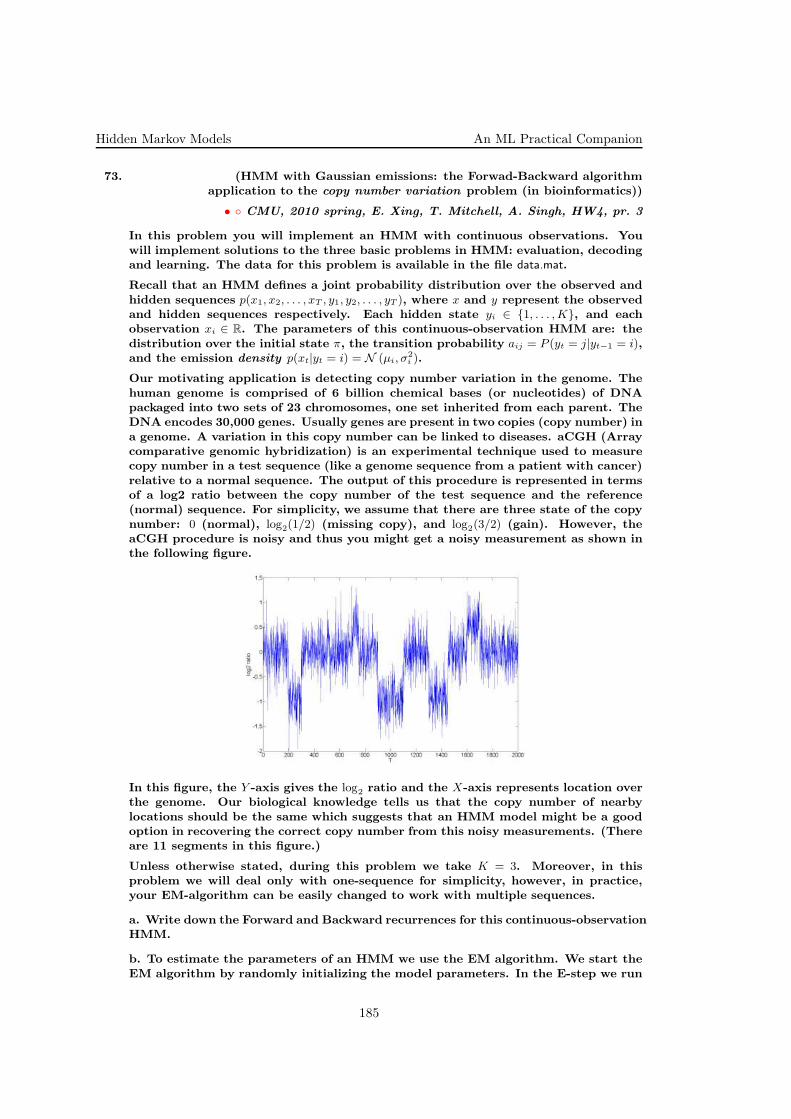
Hidden Markov Models An ML Practical Companion
73. (HMM with Gaussian emissions: the Forwad-Backward algorithmxxx application to the copy number variation problem (in bioinformatics))
• CMU, 2010 spring, E. Xing, T. Mitchell, A. Singh, HW4, pr. 3
In this problem you will implement an HMM with continuous observations. Youwill implement solutions to the three basic problems in HMM: evaluation, decodingand learning. The data for this problem is available in the file data.mat.
Recall that an HMM defines a joint probability distribution over the observed andhidden sequences p(x1, x2, . . . , xT , y1, y2, . . . , yT ), where x and y represent the observedand hidden sequences respectively. Each hidden state yi ∈ 1, . . . ,K, and eachobservation xi ∈ R. The parameters of this continuous-observation HMM are: thedistribution over the initial state π, the transition probability aij = P (yt = j|yt−1 = i),and the emission density p(xt|yt = i) = N (µi, σ
2i ).
Our motivating application is detecting copy number variation in the genome. Thehuman genome is comprised of 6 billion chemical bases (or nucleotides) of DNApackaged into two sets of 23 chromosomes, one set inherited from each parent. TheDNA encodes 30,000 genes. Usually genes are present in two copies (copy number) ina genome. A variation in this copy number can be linked to diseases. aCGH (Arraycomparative genomic hybridization) is an experimental technique used to measurecopy number in a test sequence (like a genome sequence from a patient with cancer)relative to a normal sequence. The output of this procedure is represented in termsof a log2 ratio between the copy number of the test sequence and the reference(normal) sequence. For simplicity, we assume that there are three state of the copynumber: 0 (normal), log2(1/2) (missing copy), and log2(3/2) (gain). However, theaCGH procedure is noisy and thus you might get a noisy measurement as shown inthe following figure.
In this figure, the Y -axis gives the log2 ratio and the X-axis represents location overthe genome. Our biological knowledge tells us that the copy number of nearbylocations should be the same which suggests that an HMM model might be a goodoption in recovering the correct copy number from this noisy measurements. (Thereare 11 segments in this figure.)
Unless otherwise stated, during this problem we take K = 3. Moreover, in thisproblem we will deal only with one-sequence for simplicity, however, in practice,your EM-algorithm can be easily changed to work with multiple sequences.
a. Write down the Forward and Backward recurrences for this continuous-observationHMM.
b. To estimate the parameters of an HMM we use the EM algorithm. We start theEM algorithm by randomly initializing the model parameters. In the E-step we run
185

An ML Practical Companion Hidden Markov Models
the forward-backward algorithm over the sequence(s) using the current estimateof the model parameters, and in the M-step we re-estimate the model parametersusing the expected sufficient statistics from the E-step. We repeat this two stepsuntil the log-likelihood of the observed sequence asymptotes (i.e. converges).
b.i. Using the α and β probabilities, write down the MLE estimate of πi and aij.
b.ii. Using the α and β probabilities, in addition to the observed sequences, writedown the MLE estimate of µk and σ2
k. (Hint : This is somehow similar in spirit tothe Gaussian Naive Bayes, i.e, it can be represented in terms of P (yt = i|x1, . . . , xT ).)
b.iii. Implement the EM algorithm. (You might want to refer to the problem 72.)Stop iterating when the relative change in log-likelihood (LL) falls below 1e − 3,
where the relative change in LL = |LL at iteration r - LL at iteration (r-1)
LL at iteration (r-1)|.
Run your EM algorithm over the given sequence. Initialize π and the transition ma-trix randomly (make sure they are correct probability distributions), and initializeµi by drawing it randomly from N (0, 1) and σ2
i by drawing it uniformly from [.01, 1].Repeat this experiment 5 times each of which with different random initialization.Record the final LL of each run and write down the EM-parameters for the bestand worst LL. Also draw the trace of the LL over iterations for the runs with worstand best final LL. What do you observe and why? (Note: if all your runs give thesame LL, try to initialize µ by drawing it from N (0, 2), in my implementation, I wasable to get different LL either way).
c. Decoding.Implement the Viterbi decoding algorithm. (Perform all operations in log-space toavoid under flow.)Using the estimated parameters by the EM-algorithm, run the Viterbi algorithm toget the most-probably hidden state sequence. Choose two runs from your 5-runsin (c.iv): one that gets the correct segmentation and one that doesn’t. Overlay thesegmentation of each run over the data in the previous figure. To do that, for eachpoint, draw the mean of its corresponding hidden state as recovered by Viterbi-decoding. (I am looking here for two figures, one for each run, each of which has thedata and the segmentation, please draw the segmentation with a thicker marker, i.e’linewidth’=5 in MatLab).
d. Let’s assume you don’t know the correct segmentation, did the lowest and highestLL in c.iv correspond to a correct and respectively incorrect segmentation?
e. Would you expect that a GMM with three mixtures would recover the correctsegmentation, and why? Either argue that GMM will result in the exact segmenta-tion or point to areas in the previous figure in which GMM will fail.
f. If we don’t know the correct number of states K, suggest a scheme to selectK. You shouldn’t assume that you have a reference to the correct segmentation.Moreover, assume we only have one sequence.
Solution:
a. The Forward recurrence is:
− initial: αk1 =
1√2πσk
· e−(x1 − µk)
2
2σ2k
− iteration: αkt =
1√2πσk
· e−(xt − µk)
2
2σ2k ·∑
iαit−1 aik
186

Hidden Markov Models An ML Practical Companion
The Backward recurrence is:
− initial: βkT = 1, ∀k
− iteration: βkt =
∑
i
(
aki · 1√2πσi
· e−(xt+1 − µi)
2
2σ2i · βi
t+1
)
b.i. Let γkt = P (yt = k|x1, . . . , xT ). The MLE estimate of πi is:
πi = γi1 = P (yi
1 = 1|x) = αi1 β
i1
∑
i′αi′
1 βi′
1
The MLE estimate of aij is:
αi,j =
∑
tξi,jt
∑
tγit
,
where
ξi,jt =αit aij P (xt+1|yt+1 = j) βj
t+1∑
i′,j′ αi′t ai′j′ P (xt+1|yt+1 = j′) βj′
t+1
b.ii. The MLE estimate of µk is:
µk =
∑
tγkt xt
∑
tγkt
,
where
γkt =
αkt β
kt
∑
k′ αk′
t βk′
t
The MLE estimate of σ2k is:
σ2k =
∑
tγkt (xt − µk)
2
∑
tγkt
b.iii. I ran it 5 times and the final LL’s are:
# of run final LL
1 −613.45612 −613.43653 −785.46944 −785.87055 −613.4763
So the maximum and the minimum of LL are −613.4365 and −785.8705. The parame-ters generated for those two runs are:
final LL −613.4365
µ [0.0027, 0.5664, −0.9616]
σ2 [0.1011, 0.1053, 0.1029]
π [1.0000, 4.39× 10⁻²², 3.68× 10−104]
A
0.9954 0.0016 0.00220.0145 0.9854 2.095 × 10⁻¹⁴
0.0068 3.908 × 10⁻²³ 0.9932
187
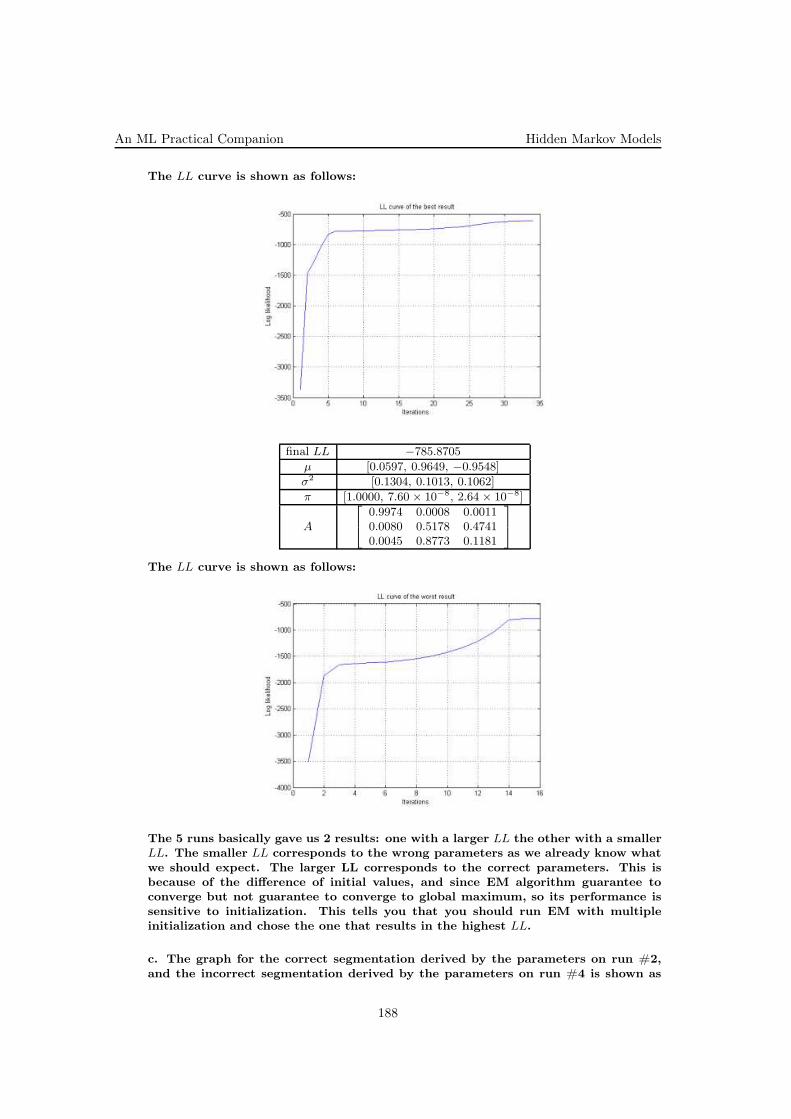
An ML Practical Companion Hidden Markov Models
The LL curve is shown as follows:
final LL −785.8705
µ [0.0597, 0.9649, −0.9548]
σ2 [0.1304, 0.1013, 0.1062]
π [1.0000, 7.60 × 10⁻⁸, 2.64 × 10⁻⁸]
A
0.9974 0.0008 0.00110.0080 0.5178 0.47410.0045 0.8773 0.1181
The LL curve is shown as follows:
The 5 runs basically gave us 2 results: one with a larger LL the other with a smallerLL. The smaller LL corresponds to the wrong parameters as we already know whatwe should expect. The larger LL corresponds to the correct parameters. This isbecause of the difference of initial values, and since EM algorithm guarantee toconverge but not guarantee to converge to global maximum, so its performance issensitive to initialization. This tells you that you should run EM with multipleinitialization and chose the one that results in the highest LL.
c. The graph for the correct segmentation derived by the parameters on run #2,and the incorrect segmentation derived by the parameters on run #4 is shown as
188

Hidden Markov Models An ML Practical Companion
follows:
d. YES. However you should be cautious that it won’t be always the case thatthe solution with the highest LL will give the correct segmentation, since here theproblem is unsupervised. In other words, we might choose a very large number ofstates that results in a very large LL but most probably we will be over fitting here.However, when we fix the number of parameters and only change the initialization,then the solution with the highest LL is always the best one for this specific choiceof K (the number of states).
e. No. GMM with 3 mixtures may not recover the correct segmentation becausethe data is noisy, and if we look at the graph where T = 600 ∼ 800, it is very hard todistinguish the pattern by GMM, because the variance is very high.
f. We can use BIC score (see lecture 8 slide 38). The idea here is to penalizecomplex models. We select K as follows: k∗ = argmaxk p(x|k)−C(x), where p(x) is themarginal LL of the observation given the number of states k, and C(k) is a complexityterm that equals to the number of parameters times lnT , where T is the number ofobservations, and the number of parameters for k states is:
k ∗ (k − 1)︸ ︷︷ ︸
transitoin matrix
+ k − 1︸ ︷︷ ︸
initial state
+ k ∗ 2︸︷︷︸
mean and variance per state – emision
189