a practical method for improved implementation of...
TRANSCRIPT

i
A PRACTICAL METHOD FOR IMPROVED IMPLEMENTATION OF PILE
DRIVING FORMULA
A thesis submitted in fulfilment of the requirements for the degree of Master of Engineering
Hamayon Tokhi
B.Eng.
School of Civil, Environmental and Chemical Engineering
RMIT University, Melbourne
February 2012

ii
DECLARATION
I certify that except where due acknowledgement has been made, the work is that of the author
alone; the work has not been submitted previously, in whole or in part, to qualify for any other
academic award; the content of the thesis is the result of work which has been carried out since the
official commencement date of the approved research program; any editorial work, paid or unpaid,
carried out by a third party is acknowledged; and, ethics procedures and guidelines have been
followed.
Signed:...................................
Hamayon Tokhi
On: 27/02/2012

iii
ACKNOWLEDGMENTS
I wish to express my deepest gratitude to my supervisor, Dr. Gang Ren, for allowing me to work on
this research. I am also grateful to him for his guidance, support and encouragement throughout the
duration of this research. I am also thankful to Professor Mike Xie for his assistance at various
stages of this research work.
My sincere appreciation is due to Dr Julian Seidel for his help in this research. His fruitful
discussions were invaluable to this work.
I am grateful to Frankipile, a local piling contractor, for allowing me for several weeks to use their
office and allowing the use of their database.
This research project contains some data provided by local, national and international organisations.
In this regard, I would like to thank the staff of the Washington State Department of Transportation
for providing support for the project.
My appreciation is also due to Professor Samuel Paikowsky from the University of Massachusetts
Lowell for providing moral support.
Finally, I would like to thank my wife Shukria; my children Nazo, Wali, Palwasha and Weis; and
my parents Fazel and Nadia. Without their support I could not have had the luxury of pursuing the
interesting research at RMIT University.
iv
TABLE OF CONTENT 1 INTRODUCTION ................................................................................................................................ 1-3
1.1 Overview ........................................................................................................................................ 1-3
1.2 Objective ......................................................................................................................................... 1-5
1.3 Scope of Work ................................................................................................................................ 1-5
1.4 Thesis Outline ................................................................................................................................. 1-5
2 BACKGROUND ................................................................................................................................... 2-1
2.1 General ........................................................................................................................................... 2-1
2.2 Pile Types ....................................................................................................................................... 2-1
2.3 Pile Material ................................................................................................................................... 2-2
2.3.1 Timber Piles ............................................................................................................................ 2-2
2.3.2 Concrete Piles ......................................................................................................................... 2-3
2.3.3 Steel Piles ............................................................................................................................... 2-3
2.4 Pile Driving System ........................................................................................................................ 2-4
2.4.1 Pile Driving Hammers ............................................................................................................ 2-5
2.4.2 Drop Hammer ......................................................................................................................... 2-6
2.4.3 Single Acting Hammer ........................................................................................................... 2-6
2.4.4 Double Acting Hammer .......................................................................................................... 2-7
2.4.5 Differential Hammer ............................................................................................................... 2-8
2.4.6 Diesel Hammer ....................................................................................................................... 2-8
2.4.7 Vibratory Hammer ................................................................................................................ 2-11
2.4.8 Hammer Cushions ................................................................................................................ 2-11
2.4.9 Pile Helmet ........................................................................................................................... 2-12
2.4.10 Pile Cushions ........................................................................................................................ 2-12
2.5 Pile Axial Capacity Evaluation ..................................................................................................... 2-12
2.5.1 Static Design ......................................................................................................................... 2-13
2.5.2 Static Load Testing ............................................................................................................... 2-14
2.5.3 Rapid Load Testing (Statnamic) ........................................................................................... 2-15
v
2.5.4 Dynamic Load Testing ......................................................................................................... 2-16
2.6 Wave Equation Analysis .............................................................................................................. 2-17
2.6.1 One-Dimensional Wave Equation ........................................................................................ 2-18
2.6.2 Boundary Conditions ............................................................................................................ 2-20
2.6.3 The CASE Method ............................................................................................................... 2-21
2.6.4 The CAPWAP Method ......................................................................................................... 2-24
2.6.5 GRLWEAP Method ............................................................................................................. 2-27
2.6.6 SIMBAT Method .................................................................................................................. 2-27
2.7 Comparative study of dynamic test methods ................................................................................ 2-28
2.8 Dynamic Formula ......................................................................................................................... 2-32
2.8.1 Rationale for use of Dynamic Formula ................................................................................ 2-36
3 LITERATURE REVIEW .................................................................................................................... 3-1
3.1 General ........................................................................................................................................... 3-1
3.2 Historical Background .................................................................................................................... 3-1
3.3 Analysis of Energy Losses ............................................................................................................. 3-8
3.4 Performance Comparison of Dynamic Formulas ........................................................................... 3-9
3.5 Pile Capacity Variations with Time .............................................................................................. 3-13
3.6 IBIS Radar .................................................................................................................................... 3-15
4 GRLWEAP Numerical Analysis ......................................................................................................... 4-1
4.1 Background ..................................................................................................................................... 4-1
4.2 GRLWEAP Inputs .......................................................................................................................... 4-4
4.3 Analysis Method ............................................................................................................................. 4-6
4.4 Results and Discussions................................................................................................................ 4-15
4.4.1 Delmag Hammers ................................................................................................................. 4-16
4.4.2 Junttan Hammers .................................................................................................................. 4-17
4.4.3 MKT Hammers ..................................................................................................................... 4-19
4.4.4 Hiley Corrections Factor ...................................................................................................... 4-21
4.5 Conclusion .................................................................................................................................... 4-23
5 FIELD STUDY ..................................................................................................................................... 5-1

vi
5.1 Test Site .......................................................................................................................................... 5-1
5.2 Site Conditions ............................................................................................................................... 5-1
5.3 IBIS Radar ...................................................................................................................................... 5-3
5.4 GRLWEAP Analysis ...................................................................................................................... 5-5
5.5 CAPWAP Analysis ........................................................................................................................ 5-5
5.6 The CASE Method ......................................................................................................................... 5-6
5.7 Field Test Results & Analysis ........................................................................................................ 5-7
5.8 Extended Application of IBIS-S ................................................................................................... 5-17
6 CONCLUSION ..................................................................................................................................... 6-1
6.1 Summary ......................................................................................................................................... 6-1
6.2 Future Research .............................................................................................................................. 6-3
APPENDIX A – Stress Wave Theory in Solid Media…………………………………A-1 APPENDIX B – Derivation of Dynamic Formula……………………………….……B-1 APPENDIX C – GRLWEAP Background Features & Parameters ………………C-1 APPENDIX D – DRIVEN……………………………………………………...…………D-1 APPENDIX E – Outputs of GRLWEAP Analysis …………………………………….E-1 REFERENCES LIST OF FIGURES
Figure 2.1 Pile support system (after Rausche et al, 1986) ............................................................................ 2-4
Figure 2.2 Pile driving hammer categories (after Rausche et al,1986)........................................................... 2-5
Figure 2.3 Operation principal of single acting hammer (PDI 2005) ............................................................. 2-7
Figure 2.4 Operation of single acting diesel hammer (after PDI, 2005) ........................................................ 2-9
Figure 2.5 Operation of double acting diesel hammer (after PDI, 2005) .................................................... 2-10
Figure 2.6 Typical setups in static load testing (after Hertlein & Davis 2006) ............................................ 2-15

vii
Figure 2.7 Wave stress propagation and reflection in pile with fixed and free end boundary conditions (after
Hertlein 2006) ............................................................................................................................................... 2-20
Figure 2.8 Schematic diagram showing typical setup of PDA (Case) method of dynamic testing (Hertlein
2006) ............................................................................................................................................................. 2-22
Figure 2.9 Simple hammer-pile-soil system for closed-form solution (after Warrington, 1997) ................. 2-23
Figure 2.10 Capacity comparisons by dynamic and static test methods (after Baker et al., 1993) .............. 2-26
Figure 2.11 Schematic diagram showing a typical setup of Simbat dynamic testing method (Hertlein 2006)2-
28
Figure 2.12 Comparative evaluation of pile movement vs. capacity by dynamic and static test methods (after
Baker et al., 1993) ........................................................................................................................................ 2-29
Figure 2.13 Capacity comparison by dynamic and static test methods (after Baker et al., 1993) ................ 2-30
Figure 2.14 Pile capacity predictions by eleven different participants (after Gozeling et al., 1996) ........... 2-31
Figure 2.15 Energy equilibrium equation relating to resistance and displacement of pile (Whitaker, 1970) .. 2-
32
Figure 2.16 Dynamic equation principle: (a) hammer, pile and soil model, (b) assumed elastic-plastic soil
response under an impact and (c) pile top movement under continuous hammer impacts (Paikowsky, 2009).
...................................................................................................................................................................... 2-33
Figure 2.17 Schematic diagram showing typical methods of measuring ‘set’ and temporary compression in
the field (Chellis 1961) ................................................................................................................................. 2-34
Figure 2.18 Measured dynamic toe resistance versus settlement for non-cohesive and cohesive soils (after
Zhang 2009). ................................................................................................................................................ 2-35
Figure 3.1 Purpose made real-time monitoring of deformation by radar IBIS-S (IDS Australia, 2009). .... 3-16
Figure 3.2 IBIS-S measurement accuracy (IDS Australia, 2009) ................................................................ 3-17
Figure 3.3 IBIS-S radar mass-spring performance test in laboratory (Bernardini, 2007) ............................ 3-18
Figure 3.4 The first 60 second of the displacement-time measurement by IBIS-S (Bernardini, 2007) ....... 3-18

viii
Figure 4.1 GRLWEAP pile, soil and driving system (hammer, helmet & cushion) modelling (PDI 2005) .. 4-2
Figure 4.2 Simplified energy balance (PDI, 2006) ......................................................................................... 4-3
Figure 4.3 GRLWEAP graphical output of results ....................................................................................... 4-15
Figure 4.4 Maximum energy versus velocity for Delmag hammer - concrete pile ...................................... 4-16
Figure 4.5 Maximum energy versus velocity for Delmag hammer - tube pile ............................................. 4-17
Figure 4.6 Maximum energy versus velocity for Junttan hammer - concrete pile ....................................... 4-18
Figure 4.7 Maximum energy versus velocity for Junttan hammer - tube pile .............................................. 4-19
Figure 4.8 Maximum energy versus velocity for MKT hammer - concrete pile .......................................... 4-20
Figure 4.9 Maximum energy versus velocity for MKT hammer - tube pile ................................................ 4-21
Figure 5.1 Generalised subsurface profile at the test site and the driving conditions analysed ..................... 5-2
Figure 5.2 A passive reflector target made at RMIT laboratory and PDA transducers .................................. 5-4
Figure 5.3 IBIS-S radar set-up and real-time monitoring of deformation ...................................................... 5-4
Figure 5.4 IBIS-S Set Measurements for Easy-Driving Condition ................................................................ 5-7
Figure 5.5 IBIS-S Set Measurements for Hard-Driving Condition .............................................................. 5-10
Figure 5.6 Match Quality and results of CAPWAP Analysis for Easy Driving Condition ......................... 5-11
Figure 5.7 Match Quality and results of CAPWAP Analysis for Hard Driving Condition.......................... 5-12
Figure 5.8 GRLWEAP Bearing Graph for Banut6T hammer ...................................................................... 5-13
Figure 5.9 GRLWEAP Analysis for easy-driving condition. Hiley Correction Factor vs. Set for Banut6T
hammer, 350mm precast pile – Easy driving condition ............................................................................... 5-14
Figure 5.10 GRLWEAP Analysis for hard-driving condition. Hiley Correction Factor vs. Set for Banut6T
hammer, 350 precast pile – Hard driving condition ..................................................................................... 5-14

ix
Figure 5.11 Overall Comparisons of Capacities by CAPWAP, Hiley, Gates, GRLWEAP and MnDOT
Methods for the Easy and Hard Driving Conditions .................................................................................... 5-15
Figure 5.12 GRLWEAP Analysis. Hammer performance and efficiency for Banut 6t ............................... 5-16
LIST OF TABLES
Table 2.1 Summary of advantages and disadvantages of different pile types (after Broms, 1981) ............... 2-2
Table 2.2 A summary of the some of the static capacity evaluation methods for driven pile (Paikowsky et al
2004). ............................................................................................................................................................ 2-13
Table 2.3 Advantages and disadvantages of dynamic methods (Paikowsky, 2004) .................................... 2-26
Table 3.1 List of most commonly used dynamic formula (after Fragaszy et al., 1988) ................................. 3-4
Table 3.2 Pile driving formulas investigated and new Mn/DOT formula proposed by Paikowsky (2009) ... 3-7
Table 3.3 Typical analysis of driving formula to include energy losses (Chellis 1951) ................................ 3-8
Table 3.4 Safety factors for dynamic methods (after McVay and Kuo 2000) .............................................. 3-10
Table 3.5 Recommended safety factors for dynamic methods (after McVay & Kuo 2000) ........................ 3-11
Table 3.6 Comparison of results by Fragaszy et al. (1988) .......................................................................... 3-12
Table 3.7 Performance of dynamic test methods (Paikowsky et al., 2004) .................................................. 3-13
Table 3.8 Empirical equations presenting pile capacity change over time Komurka et al (2003) ............... 3-14
Table 4.1 A summary of hammer, pile and soil type combinations in the study ........................................... 4-7
Table 4.2 Hammer Details .............................................................................................................................. 4-7
Table 4.3 Hammer and Pile Cushion Details ................................................................................................. 4-9
Table 4.4 Sample of the database from GRLWEAP analysis ........................................................................ 4-9
Table 4.5 Soil combinations and cross-section profiles used in the GRLWEAP analysis ........................... 4-10
x
Table 4.6 GRLWEAP resistance parameters for ST analysis for cohesion-less soils .................................. 4-10
Table 4.7 GRLWEAP resistance parameters for cohesive soils ................................................................... 4-11
Table 4.8 GRLWEAP recommended Quake values for driven piles ........................................................... 4-11
Table 4.9 GRLWEAP recommended damping values for driven piles ........................................................ 4-12
Table 4.10 Input parameters in DRIVEN ..................................................................................................... 4-12
Table 4.11 DRIVEN output of skin and end bearing capacities for precast concrete pile ........................... 4-14
Table 4.12 DRIVEN output of skin and end bearing capacities for tube pile .............................................. 4-14
Table 4.13 Summary of range of Hiley Correction Factors for various driving system and soil types ....... 4-22
Table 4.14 Statistical analysis of HCF based on the GRLWEAP data for each hammer type ..................... 4-23
Table 5.1 Results of field testing .................................................................................................................... 5-8
Table 5.2 Soil parameters derived from signal matching CAPWAP ............................................................. 5-9
Table 5.3 Correction factor calculations based on the field set measurement by Ibis-s .............................. 5-16

xi
LIST OF PUBLICATIONS
Tokhi H., Ren G., Xie Y.M. (2011), Improving the Predictability of Hiley Pile Driving Formula in
the Quality Control of the Pile Foundation, Advanced Materials Research, Volume 261-263, pp.
1290-1296.
Tokhi H., Ren G., Xie Y.M. (2011), A new application of Radar in Improving Pile Dynamic
Formula used in the Quality Control of Pile Foundation, Australian Geomechanic Society (AGS),
Volume 46, Issue 4 , pp. 35-49, December 2011.
NOTATION All notations and all symbols are defined where they first appear in the text. For convenience, they
are also listed here together with their definitions. Metric units according to the S.I. system have
been used.
a acceleration;
Ap cross sectional area of pile;
As pile shaft area;
C velocity of wave propagation in pile material;
C1 temporary compression in the pile cap;
C2 temporary compression in the pile;
C3 temporary compression in the soil (or rebound);
Cu undrained shear strength;
E coefficient of restitution;
eh hammer efficiency;
ed driving system efficiency;
Eh, En, Er rated energy of hammer;
Ep modulus of elasticity for pile material;
Epl energy losses in pile;
Esl energy losses in soil;
Emax maximum energy entering a pile;
F1 pile head force at the peak impact or other time;
F2 pile head force at the wave return time or (2L/c) after the F1;

xii
fs soil friction resistance;
g acceleration due to gravity;
h actual stroke or height of hammer drop;
H maximum stroke;
I element number;
Jc case damping factor;
Js shaft damping factor;
Jt toe damping factor;
l, L length of pile;
v particles velocity of the material around their points of equilibrium;
V1 pile head velocity at the peak impact force;
V2 pile head velocity at a time 2L/c later than V1 time;
vi velocity of ram, at moment of impact= 2𝑔𝑒 ℎ𝑊 𝑊⁄ .
vc velocity of ram and pile, at end of compression period;
vr velocity of ram at end of period of restitution;
vp velocity of pile at end of period of restitution;
Mr moment of ram, at moment of impact (=Wrv/g);
Mt amount of impulse causing compression;
eMt amount of impulse causing restitution;
P1 the peak impact force;
P2 impact force at a time 2L/c later than P1;
Pp pile perimeter;
qs shear stress;
qu unconfined compressive strength;
Qs shaft quake;
Qt toe quake;
Ru ultimate carrying capacity of pile (ultimate soil resistance);
R safe (factored) working load;
s permanent pile penetration or set;
t time;
t1 first peak, or impact time on a force vs time curve from the PDA testing results;
t2 wave return time or 2L/c later than t1;
Wr weight of ram;

xiii
Wp weight of pile;
Z vertical distance along pile axis;
Z impedance = AE/c=Aρc;
φ friction angle;
γ weight density;
ρ mass density;
σ stress;
DEFINITION OF TERMS & ABBREVIATIONS Bl.Ct: Blow count (blows/m) =1000 𝑆𝑒𝑡 (𝑚𝑚)⁄ .
Bl.Rt: Blow rate (blows/minute).
BN: Blow number.
BOR: Beginning of restrike.
CAPWAP: Case Pile Wave Equation Analysis Program.
ComStr: Compression stress.
COR: Coefficient of restitution, it describes the energy absorption of
material= ℎ ℎ⁄ 𝑤ℎ𝑒𝑟𝑒 ℎ & ℎ 𝑎𝑟𝑒 𝑖𝑛𝑖𝑡𝑖𝑎𝑙 𝑎𝑛𝑑 𝑓𝑖𝑛𝑎𝑙 ℎ𝑒𝑖𝑔ℎ𝑡𝑠.
COV: Coefficient of Variation. It is a non-dimensional parameter that denotes the
relative natural scatter of data. COV=Standard Deviation/ Mean.
Compression (c): Temporary compression or pile rebound as a result of hammer blow.
DFN: Final displacement (PDA result).
DMX: Maximum displacement (PDA result).
Driving Formula: Energy equation developed based on the Newtonian theory to predict pile
capacity as a function of delivered energy to pile, pile set and temporary
compression.
Enthru: Transferred energy into a pile.
EMX: Maximum measured energy with PDA device.
EOD: End of driving.
EOID: End of initial drive.
FOS: Factor of safety. It is used account for uncertainties from loading conditions,
site variation and other geotechnical parameters.
GRLWEAP: Goble-Rausch-Liking Wave Equation Analysis Program.

xiv
IBIS-S: Relatively new radar equipment used in civil engineering applications, such
as bridges, towers and high rise buildings. It was used in piling application
for the first time and it can measure pile velocity, displacement, pile set and
delivered hammer energy accurately and safely.
Kinetic Energy: Potential Energy x Efficiency=ℎ𝑊 × 𝑒 .
LVDT: Linear variable differential transformer. It is used for measuring linear
displacement.
maxCForce: Maximum compression force.
maxCStrss: Maximum compression stress.
maxD: Maximum displacement.
maxEt: Maximum transferred energy.
maxTForce: Maximum tension force.
maxTStrss: Maximum tension stress.
maxV: Maximum velocity.
MQ: Match Quality. A number that measures the quality of measured and
calculated quantities such as acceleration and force propagation in pile.
Pile: Pile is an elongated columnar body made from concrete, steel and timber that
is driven in ground to transfer vertical loads to deep below ground.
Pile Driving Rig: Rig used to drive piles. There are many types of rigs available and their
differences are mainly due to the types of hammer used.
PDA: A relatively expensive pile testing method called Pile Dynamic Analysis.
Accelerometer and strain sensors are attached to the pile and the signals are
captured via a portable computer. A software program uses one-dimensional
Wave Equation to match the signals and hence calculate the pile capacity.
Penetration: Total depth of embedment of pile in the ground.
Potential Energy: Actual drop height ×Wr= ℎ𝑊 .
PLT: Pile load test.
Rated Energy: Maximum energy a hammer can deliver=𝐻𝑊 . Set: Permanent pile penetration per hammer blow.
SLT : Static load test.
SPT: Standard penetrometer test.
TC: Temporary compression (PDA result)
TenStr: Tension stress.

1-1
ABSTRACT
Piles are widely used in construction of foundations for infrastructure such as buildings, bridges and
offshore structures particularly at fill and soft soil sites. Hence accurate and reliable determination
of pile capacity is very important for design, construction and the overall estimate of the cost of
these foundations. It is common in design practice to predict pile capacity by static analysis in
advance of pile driving based on the results of in-situ and laboratory tests. Static load testing is
carried out during construction stage on a typically 2-5 per cent of the piles in a reasonably large
project to determine ultimate load carrying capacity of pile. One of the oldest methods of pile
dynamic testing is the use of dynamic formulae that were developed based on the Newtonian impact
theory. The contemporary dynamic methods are based on the application of the stress wave theory
to piles, whereby the dynamic testing measurements of force and velocity at the upper end of the
pile during pile driving and restrike are used for pile capacity prediction. This dynamic testing by
wave equation analysis is a prevalent method of pile capacity and driving stress calculations.
Unfortunately, though dynamic methods have been used in practice for many years, actual
reliability of dynamic methods is vague because their comparison with static loading tests is made
incorrectly in most cases due to the variation of pile capacity with time after the initial driving.
On the other hand, the traditional energy or dynamic formulae have been regarded as being
unreliable and less accurate than the more analytical methods based on the wave equation analysis.
The main two reasons for the poor performance of the dynamic formulae are the assumption of
hammer energy and the inherent flaw that they do not take the dynamic resistance into account.
With the advent of new technologies in the construction industry, gradual improvements have been
made in the application of the dynamic formulae in many projects that have resulted in greater
reliability. This research attempts to improving the reliability of the dynamic formula by accounting
for the hammer energy and the dynamic resistance by carrying out a comprehensive GRLWEAP
parametric analysis for different hammers, soil and pile types. Also, a new application of radar
called IBIS-S is proposed as well as a site test results are presented using the Hiley, Gates and
MnDOT formulae. The comparison of the results with the more rigorous PDA, CAPWAP® and the
GRLWEAP™ analysis show that with the application of new and precise testing equipments, the
dynamic formula can be used with greater accuracy than the Case method. It is also shown that the
IBIS-S unit may also be used to estimate and evaluate the empirical parameters used in the

1-2
CAPWAP® and GRLWEAP™ analysis. This approach enables evaluation of the pile capacity to be
made more accurately using the dynamic equations.

1-3
CHAPTER 1
1 INTRODUCTION
1.1 Overview
Casagrande (1964) recalled a prediction, made by Karl Terzaghi, in 1964 on the first anniversary of
his death that:
‘..the worst enemies of soil mechanics would not be those who were denying the validity of its basic
assumptions, because those would die out, but that the worst harm would be done when pure
theoreticians discovered soil mechanics, because the effort of such men would undermine its very
purpose.’
Piling works also happen to fall in the same field because of the heavy reliance on the geotechnical
engineering discipline. In fact piling work is a harmonious mix of art and engineering knowledge.
For thousands of years since piles were first used by humans, they naturally searched to developed
ways to estimate the loading capacity of pile once it is in the ground in the most efficient and
economic manner. One of the oldest methods is the Dynamic or Energy Formula that is still in
common use amongst the piling practitioners and consultants according to research surveys
(AbdelSalam et al., 2009, Fleming K. et al., 2008).
The early users of the pile driving formula applied the idea of driving a stake to driving of a pile and
made the assumption that the effort required to drive the stake is directly related to the resistance

1-4
provided by the ground (Whitaker, 1970). As a result, many empirical formulae termed ‘dynamic
formulae’ have been derived to establish the relationship between the pile driving resistance or
penetration under hammering and the ultimate bearing capacity of pile.
Pile Dynamic or Energy Formula is a term used to describe a range of formulas of which
Engineering News (ENR), Danish, Gates, Janbu, Hiley, FHWA and WSDOT are well known
among many others. Countries with a strong tradition of using the Hiley Formula are particularly
Hong Kong, UK and Australia while Gates, Janbu, FHWA and WSDOT are commonly used in the
US. (Fung W.K., 2004, Lowery L.L. J r . et al., 1968, Whitaker, 1970)
These dynamic equations are generally categorised into theoretical equations, empirical equations
and those consisting of the combination of the two. The theoretical basis for the derivation of the
pile driving formulas is based on the Newtonian principles of impact between two rigid bodies, for
example the driving hammer and the pile. Thus driving formulas are simple idealisation of complex
interactions between hammer, pile and the ground.
Experience and pile tests over the years have shown that the dynamic formulae in general and the
Hiley formula in particular, consistently over predict pile capacity compared to the reference static
tests. It is particularly true when the safety factors are applied to the ultimate load calculated by the
dynamic formulae. Typically, a safety factor for the Hiley formula is around 3 whilst for the Wave
Equation Method it is 2.5 and for static load tests it is about 2 (Paikowsky, 1994, Paikowsky S,
2004, Paikowsky S., 2009). The reason for this over prediction of capacity evaluation by the Hiley
formula is that the formula does not take into account the dynamic component of the capacity.
The primary aim of this research is, therefore, to improve the reliability of the dynamic formula.
This research program will concentrate on the proposal of a correction factor to adjust for this
dynamic component similar to the damping parameter used in the Wave Equation Analysis and
validate its reliability experimentally and theoretically. Similarly, the issue of the variation in the
hammer energy delivered to pile needs to be improved by the adoption of new technology and
validate experimentally.

1-5
1.2 Objective
The objectives of this research are:
1. To review and summarise the methods of the pile driving formula and derive a more general
method of application.
2. To improve the reliability of the dynamic formula by accounting for the hammer energy and
the dynamic resistance by carrying out a comprehensive parametric analysis using wave
equation analysis software for various hammer, soil and pile types.
3. To propose a new application of radar instrument called IBIS-S.
4. Carry out empirical analysis of site test results using the Hiley, Gates and MnDOT formulae.
5. Perform PDA, CAPWAP® and the GRLWEAP™ analysis and compare the results.
6. To illustrate that the dynamic formula, particularly the Hiley formula, can be used to show
that with the application of new and precise testing equipments.
7. To show the dynamic formula can be used to determine the ultimate loading capacity of
piles.
1.3 Scope of Work
The following paragraph provides a summary of the scope of work that has been undertaken during
this research study.
• Piling Database: Data collection and analysis of piling contractor’s database.
• Software analysis: Wave equation analysis of 1400 cases.
• Field testing: Parallel testing of pile using PDA and IBIS-S instruments.
• CAPWAP: Wave equation signal matching analysis of the field testing results.
1.4 Thesis Outline
This thesis is presented in seven chapters. After the background and objectives of this research in
earlier sections, progression towards the proposed research work is presented in the following order:

1-6
Chapter 2 Background
This chapter is presented in the context of pile dynamic methods and in relation to pile driving
formula.
Chapter 3 Literature Review
This reviews relevant previous theoretical and experiment works into the pile dynamic formula,
including pile testing and installation methods.
Chapter 4 Wave Equation Analysis of Piles
Provide a comprehensive parametric data analysis using wave equation based finite element
analysis package named GRLWEAP. Theoretical relationships between energy and pile movement
(set) for different hammers, piles and ground conditions are presented.
Chapter 5 Field Instrument Results and Analysis
Present the results of field dynamic testing and analysis by wave equation with respect to the
objectives of the research. A new application of radar instrument for pile testing is proposed and the
results of parallel testing with the field dynamic testings are presented.
Chapter 6 Summary and Conclusions
The results of the research program are summarised and conclusions drawn.
Recommendation for future research work and some issues raised in this research are suggested.

2-1
CHAPTER 2
2 BACKGROUND
2.1 General
In order to present the setting for this research, it is deemed necessary to present a discussion on the
application of different dynamic pile testing methods in practice with particular emphasis on the
dynamic formula, which is the particular subject of presented research. The methods are divided
according to the design and construction stages of a project. The methods that require dynamic field
measurement, which is based on the wave equation, can be broadly categorised as those that are
based on a simplified analysis and those that are based on further elaborate computer signal
matching calculations. Finally, a brief discussion of pile driving equipment is given to complete the
setting of the presented research.
2.2 Pile Types
Pile foundations are employed in various situations where the weight of a superstructure need to be
transported to stronger soil layers deep underground. It is the best foundation solution in areas prone
to erosion and earthquake and also is the only possible foundation option for offshore structures.
Piles are generally categorised as displacement and non-displacement piles. Driven precast and
close-ended tube piles fall into the displacement category, in which, large volume of soil is
displaced during installation. Steel piles with thin cross sections such as H and open-ended tube as
well as screw and bored piles are categorised as non-displacement piles. These piles cause little or

2-2
no disturbance to the surrounding soil during piling process. A summary of advantages and
disadvantages of different pile types are presented in Table 2.1.
Table 2.1 Summary of advantages and disadvantages of different pile types (after Broms, 1981)
2.3 Pile Material
Depending on the applicability in a given situation, one of the three different pile types timber,
concrete or steel is selected to construct a pile foundation.
2.3.1 Timber Piles
Timber is well suited for construction of jetty and other on-shore structures for their energy
absorbing qualities. They relatively inexpensive pile construction material and its durability and
resistance to decay can be improved with preservatives such as arsenates and creosotes or can be
even shotcreted. All the methods of application of preservative are the same in principle. The piles

2-3
to be treated are loaded into a large steel cylinder and preservatives are applied under pressure until
the required absorption has been obtained.
The main drawback of timber pile is the limit of length and structural capacity. It is therefore the
most suitable option for the construction of residential building in marshland area and marine
environment. In US and Scandinavian countries both softwood and hardwood are still commonly
used. In Australia treated hardwood is commonly used. Pile lengths vary up to 15m and pile
sections are generally square (250mm-500mm) although round section can be also be used.
Driving of timber piles are carried out with a drop or light hydraulic hammers. For driving through
dense soil, a steel band around the head and shoe attached to the tip of the pile are needed to
mitigate against head crushing and toe disintegration.
2.3.2 Concrete Piles
Concrete piles are the most versatile and are useful in carrying fairly heavy loads through soft soil
to harder strata. Concrete piles can be cast to a specification on site or at a yard. The main two types
of concrete pile are precast and cast in-situ. Precast piles are normally constructed in square
constant cross section, or circular with a core hole to save weight. Pile tips may be flat or pointed
and it can also adopt a mechanical shoe for hard driving conditions. Concrete piles can be spliced to
suit any desired length by mechanical means.
2.3.3 Steel Piles
These types of piles can come in many different sections such as tube, H or I-sections and provide
excellent resistance to both compression and tensile forces. Steel piles are less prone to structural
damage during driving process and can be spliced to a desired length very conveniently. However,
the main disadvantages of steel piles are relatively high cost and vulnerability to corrosion in
marine environments.

2-4
2.4 Pile Driving System
Piles are nowadays installed by driving, drilling, vibration, screwing, jacking or by a combination
and can be augmented by excavation or water jetting. Installation of piles by brutal force requires
careful control combined with good deal of experience and judgment. Hence, success depends
heavily on the selection of pile driving equipments, hammers, cushion materials as well as a
sufficient knowledge of the soil conditions.
Generally the pile driving system consist of lead, hammer cushion, helmet and pile cushion as
shown in Figure 2.1. Different lead system are designed and used depending on the situation one
site. It is mainly categorised into fixed, semi-fixed and offshore lead.
Figure 2.1 Pile support system (after Rausche et al, 1986)

2-5
2.4.1 Pile Driving Hammers
Piling hammers play the most important role in the installation of piles because the capacity of the
pile depends on the performance of the hammer. The essential role of a hammer is to impart kinetic
energy resulting from the gravity fall of the hammer weight. In some hammers this energy is
augmented by taking advantage of gravity and further accelerating the mass by mechanical means.
However, not all potential energy is converted to kinetic energy and there are losses in driving
mechanism due to friction, cushioning and the restitution.
Hammers are categorised into "external combustion", meaning that the power to raise the ram
comes from an external source such as rope, steam, air, hydraulic and "Internal combustion" that
only apply to diesel hammers. There are further subcategories and Figure 2.2 gives a hierarchy of all
common hammer types.
Figure 2.2 Pile driving hammer categories (after Rausche et al,1986)
The efficiency of a diesel hammer, in contrast to the hydraulic hammer, depends on the soil
resistance, mass and stiffness of the piles because the ram relies on the reaction force to be lifted up.
It is for this reason that the diesel hammers have an advantage over other hammers when driving

2-6
concrete piles due to the low impact energy in low resistance soils as it minimises potential
damaging tension stresses. Another concern with diesel hammers is that the impact energy may
suddenly increase and over-stress the pile. This can be a concern when driving piles through very
soft soil to a hard rock bearing layer.
2.4.2 Drop Hammer
A drop hammer is essentially a weight that is repeatedly raised by a rope and then released by
tripping it to fall on piles by gravitational force. Dropping weight or drop hammer is the traditional
method of pile driving and is still frequently used. A track rig or crane can incorporate the guide for
a drop hammer and hoist the pile into position and support it during driving. The impact velocity or
delivered energy is strongly influenced by frictional losses in the hoist rope and guide frame.
2.4.3 Single Acting Hammer
Single acting hammer uses steam or air to raise the ram that is connected by a rod to a piston inside
a cylinder, shown in Figure 2.3. On upstroke, the steam or air pressures forces the piston up through
an inlet valve. When the piston reaches the top of the cylinder near a vent, the valve trips and closes
the inlet and opens the cylinder to the exhaust port, which results in hammer falling and driving the
pile. These hammers usually have a 0.9m stroke. The blow characteristic is low impact velocity that
is more effective than a high-velocity light ram.

2-7
Figure 2.3 Operation principal of single acting hammer (PDI 2005)
2.4.4 Double Acting Hammer
As the name implies, double acting hammers use air, steam or hydraulic to drive the hammer ram
both in the up and down strokes. Thus the energy developed is a direct result of gravity fall plus the
force developed in the piston by air, steam or fluid pressure. These hammers operate at a high speed
compared to the single-acting hammers. However, because the maximum kinetic energy cannot be

2-8
more than the stroke times the weight and the hammer weight less than that of a single-acting
hammer due to speed of operation, it has led to the development of differential hammers.
2.4.5 Differential Hammer
Differential hammer is similar to double-acting hammer that uses air, steam hydraulic pressure to
raise the ram and accelerate the fall of hammer. However, it differs from the double-acting hammer
in that it has two pistons located at approximately the top and middle of the cylinder. The upper
piston is larger than the lower piston thus the difference in pressures on these two pistons is the net
driving force of the ram. The use of heavier rams in the differential hammers result in the advantage
of differential hammers over double acting hammers. For hydraulic hammers, only one piston is
required to the high operating pressure.
Air and steam differential hammers tend to run slowly in easy driving conditions and increase their
speed as the pile resistance increases. For hydraulic hammers, on the other hand, the operating
speed is high during easy driving conditions and slows down as the pile resistance increases.
Overall, the operating speed of hydraulic differential hammer is 1.5 times the comparable air or
steam differential hammers.
Differential hammers can show variability in performance and the ram velocity is affected by the
throttle control. The maximum energy developed by these types of hammers cannot exceed the
hammer weight times the drop height (PDI 2005).
2.4.6 Diesel Hammer
Diesel hammers are either open-ended (single-acting) or closed-ended (double-acting) type. As the
name implies, for the open-ended hammer the top of the cylinder is open, therefore, allowing the
piston to rise and then to freely fall by gravity. A diagram showing the working principle of the
single acting hammer is shown in Figure 2.4. The basic working principle of the diesel hammer is an
internal combustion of diesel fuel between the ram and anvil that results in both pushing the pile
down and in raising of ram for the next stroke. The cycle begins by raising the ram by a lifting
device inside the cylinder and then allowed to fall. As it falls, the exhaust valves are closed off and
diesel fuel is pumped into the combustion chamber. The falling ram compresses the mixture of air

2-9
and fuel and upon impact of the ram with anvil, the compressed hot air-fuel mixture is ignited that
result in the downward pushing of the pile and the upward moving of the ram for the next stroke
cycle.
Figure 2.4 Operation of single acting diesel hammer (after PDI, 2005)

2-10
The closed-ended diesel hammers operate similarly to open-ended hammers, except, that for the
closed-ended hammers, the air above the piston is compressed on the upstroke and it accelerates the
ram or piston down as it expands. The pressure generated in the top chamber can be monitored and
converted to an equivalent stroke. Figure 2.5 shows a schematic arrangement of the double-acting
diesel hammers.
An interesting feature of some diesel hammers is that the single and double acting hammers are
convertible. These hammers generate maximum energy under hard driving conditions. The hammer
impact can be affected by abnormal pre-ignition which can be caused by either overheated ram or
using fuel with low flash-point. The diesel hammers operate at approximately similar speed to the
single-acting hammers.
Figure 2.5 Operation of double acting diesel hammer (after PDI, 2005)

2-11
2.4.7 Vibratory Hammer
Vibratory hammer consists of contra-rotating eccentric masses that are powered by hydraulic or
motor and can be supplied from a mobile generator or hydraulic power pack. The vibrations are
produced by the pair of weights mounted on rotating shafts and phased in a fashion that tends to
cancel the horizontal forces and to add in the vertical direction. The pile vibrators generally operate
at low frequency, below 50Hz with un-damped amplitude of 5 to 30mm or high frequency that
operate in the range of resonant frequency of the pile itself (Chellis, 1951, Fleming K. et al., 2008,
Salgado R., 2006, Tomlinson, 2001). During vibrating process, granular soil around the pile
effectively become like fluid resulting in reduction of shaft friction and improved penetration. For
clay soils, however, the effectiveness of the vibratory hammer is generally not good. The main
drawback of the vibratory hammer is associated with large energy inputs that are put into pile that
results in excessive noise and vibration. It can be a good method to extract piles from the ground.
Vibratory hammers are not modelled by the existing wave equation analysis. One of the main
disadvantages of the vibratory hammers is that these types of hammers are not yet able to be
modelled and analysed by the existing wave-equation methods.
2.4.8 Hammer Cushions
Hammer cushions are used between the helmet (also called cap) and the ram to protect the ram and
pile from damage and also to control impact stresses. Commonly used hammer cushion material
consist of hardwood about 150mm thick in tight fitting steel ring with its grain parallel to the pile
axis to provide maximum stiffness. However, the disadvantages of this cushion are that it becomes
crushed and burnt, requiring frequent replacement, and the elastic property of the material changes
during driving.
Instead, laminated aluminium and micarta materials are frequently used. These cushions have a
consistent energy transmission, elastic property remain nearly constant and have relatively long life
compared to the hardwood cushions. As a result, the coefficient of restitution or the efficiency of
these cushions is about 0.8 compared to 0.5 for hardwood cushions.

2-12
2.4.9 Pile Helmet
Pile helmet is used to hold the head of the pile in position under the ram, to distribute the impact
force and align the hammer and the pile. Helmets for H and tube piles are normally snugly fitted to
prevent bulging and distortion. However, for concrete piles it should not be tight to prevent pile
rotation. Pile drivability is heavily influenced by the mass of the helmet.
2.4.10 Pile Cushions
Pile cushions are used between the pile helmet and the top of concrete pile. It is intended to protect
the pile and control impact stresses in the pile. Pile cushions are made from plywood and it is
designed to prevent concrete spalling and to limit excessive stresses and yet transmit the hammer
impact energy efficiently to the pile. Therefore, it is prudent to achieve a balance between the
hammer size, cushion thickness and the pile size.
2.5 Pile Axial Capacity Evaluation
From start to finish, construction of pile foundation generally involves four stages: geotechnical site
investigation and associated laboratory testing; design of pile load carrying capacity based on the
numerous analytical methods; installation; and pile capacity verification as well as the load-
settlement performance and integrity. Pile test may be carried out at any stage of construction
whether it is during, preconstruction or post construction. At preconstruction stage, the design of
pile capacity is based on the site investigation and laboratory testing that are inherently uncertain
and over simplified. Hence it becomes necessary to test piles to ensure compliance is met to the
required capacity. Static testing is carried out on insignificant percentage of installed piles (1 to 2%)
due to the high cost of testing involved. Other testing like dynamic testing is often undertaken on
relatively higher percentage of installed piles (5-10%) (Fleming K. et al., 2008, Hertlein B., 2006,
Salgado R., 2006, Timoshenko S.P., 1951). Therefore, dynamic testing eliminates some of the
uncertainties in the inherent deficiencies in the design processes. The remaining untested piles (90
to 95%) of piles are installed based on the results of the dynamically tested piles. This is precisely
one of the biggest disadvantages of dynamic testing and it is therefore the main justification for the
important role of the dynamic formula. This is the main focus of current research. In the following
sections, both the traditional and the more recent methods of determining pile capacity are

2-13
discussed, with particular emphasis on dynamic pile testing as it relates to the specific focus of the
research undertaken.
2.5.1 Static Design
A pile subjected to vertical load will carry the load partly by shear generated along the shaft and
partly by normal stresses generated at the base of the pile. Currently numerous analytical methods
for calculating ultimate static capacity have been developed. Some of the methods that are used for
calculating pile capacity are Terzaghi, Meyerhoff, Vesic, the α , β and λ methods. Table 2.2 gives a
summary of the equations used in the different methods. It needs to be emphasised that all of these
methods are formulated on in-situ soil parameters, which are often very hard to know with certainty
and to account for the variation of capacity with time. More comprehensive details on these
methods can be found in Tomlinson (2001). The ultimate load derived from these equations is
divided by a suitable factor of safety (FOS) to obtain allowable load on a pile that is subject to an
allowable settlement. The magnitude of FOS is dependent on several factors and a FOS between 3
and 4 is commonly used.
Table 2.2 A summary of the some of the static capacity evaluation methods for driven pile (Paikowsky et al
2004).

2-14
2.5.2 Static Load Testing
Static load testing began as a way to check that piles could carry their load as designed. The test
consists of applying a load equal to the working load plus an equivalent FOS load to the pile top in
a manner in which incremental load is applied and held for duration of time and then taken off in
similar fashion. The load on pile is made up of heavy load available close to site, usually stacked on
a frame called kentledge. Other systems are ground anchors and reaction piles. Figure 2.6 shows a
typical set up of the reaction system.
Static load testing is normally undertaken for the reasons of establishing the load-settlement
relationship, proof testing to ensure failure is not reached and to check the capacity evaluation by
other dynamic and static formula to enable other piles to be installed by empirical methods. It is for
these reasons that static load testing is often used as a reference for comparisons of pile capacity
evaluations because of the assumption that the testing closely replicates the process of pile loading
on a construction site.
However, static load testing can inflict a high cost a significant amount of time right from set up
and dismantle to interpretation of results. In addition, the need for significant reaction system
imposes even higher cost. Despite all these, the results are often very difficult to interpret by the
current methods of analysis. The methods used to calculate the pile capacity from the static load
testing are Davison, Chin, Butler-Hoy, Tangent, Slope, D/10 (Allen T. M. , 2005, Allen T. M.,
2007, Fleming K. et al., 2008, Fragaszy R.J. , 1988, Fragaszy Richard J. , 1989, Gozeling F.T.M and
Van Der Velde E.G., 1996, Lowery L.L. J r . et al., 1968). These methods often give different
results which make the interpretation very difficult. In situations of constructing pile in an offshore
environment, it may be very difficult to perform static load testing.

2-15
Figure 2.6 Typical setups in static load testing (after Hertlein & Davis 2006)
2.5.3 Rapid Load Testing (Statnamic)
Statnamic load testing combines the advantages offered by both static and dynamic load tests. It
uses rapid compressive force and the parameters like acceleration and displacements are measured

2-16
with accelerometers and displacement transducers. The Statnamic device itself consists of a large
mass and a combustion chamber in which a rapid burning fuel is fired to create a compressive force
on the pile. The returning mass is caught by a mechanical system before it impacts the pile again.
During the short loading, over 2000 data are taken by a data acquisition device and load-
displacement curve generated is used to determine the equivalent static load.
Generally, the peak impact velocity generated during Statnamic testing is less than the dynamic pile
testing. If the rapid burning fuel is excessive, then the impact velocity may be quite large, thus,
resulting in an overestimate of static capacity.
2.5.4 Dynamic Load Testing
This method of determining the pile capacity was developed in the 1970’s (Rausche F. et al., 1972).
Today, dynamic pile testing is accepted as a valid technique of inferring the static capacity of piles
and a standard quality assurance and construction control method for piled foundations. A typical
set-up for carrying out a dynamic test involving a ram as well as strain gauges and accelerometers is
shown in Figure 2.8.
The dynamic pile testing method is based on the analysis of stress-wave propagation in pile
generated by the blow of the pile driving hammer, and reflected from soil resistance acting along
and below the pile and from variations in the geometry and material properties of the pile. The
theory of stress-wave propagation in the pile is well documented e.g. (Rausche F. et al., 1972,
Randolph M.F., 1979, Goble G.G. & Aboumatar H., 1992, Rausche et al., 1997, Hussein M.H.,
2004, Fleming K. et al., 2008). An extract from Timoshenko (1951), Verruijt (2005) and PDI inc.
(2006) that explain critical and relevant aspects of the theory is included in Appendix A.
Dynamic pile testing has become widely used as a replacement for or supplement to static loading
tests because of its inherent savings in cost and time. These dynamic methods allow monitoring pile
driving and restrike, and also provide a method of identifying problems during driving for many
kinds of piles. To obtain reliable ultimate resistance, it is necessary that the long term pile capacity
be fully mobilised. Dynamic testing methods can determine static capacity at the time of testing, in
other words either at the end of driving or at restrike. This is a substantial advantage because

2-17
dynamic tests can be easily repeated and, consequently, there is an opportunity to obtain pile
capacity as a function of time as well as pile embedment.
A special advantage of dynamic pile testing that is not available to static load testing is the ability to
test the pile during the exact time of installation. Hence, since piles are installed in soils of all types
particularly fine-grained soils below the water table, the piles experience time-dependent capacity
changes. Capacity increases (known as set-up, presented in next Chapter 3) are most common. Also,
capacity reductions (known as relaxation) are observed in relation to loss of toe capacity in
shale/chalk formations. These capacity changes can be monitored by a sequence of dynamic tests
commencing at the end of driving, and continuing for days, weeks or even years. Practical
limitations make it impossible to statically load test a pile at the completion of installation, or to
undertake sequential load tests, unless for a special research application. This feature of dynamic
testing enables a direct relationship to be established between pile capacity and the field response
(measured as set and temporary compression), and to develop a meaningful correlation between
dynamic pile testing and dynamic formulae. Dynamic testing is used not only for estimating pile
capacity, but also more generally for construction control, including stress control, damage
assessment and pile driving hammer evaluation.
When a pile is dynamically tested during driving or after installation, the capacity of the pile can be
approximated using a non-rigorous method called the Case Method and/or more accurately
determined using a rigorous method involving signal matching of the measured stress-wave record.
These analyses are described subsequently.
2.6 Wave Equation Analysis
The theory of wave propagation provides the proper theory of pile driving. Wave equation was
proposed nearly 150 years ago in 1866 by Saint Venant and Boussinesq for longitudinal impact of
bars (Timoshenko and Goodier, 1951). Isaacs (1931), an Australian, was the first to point out the
application of wave propagation theory to piles and developed a set of graphical charts and
formulas to analyse the stresses and displacements in piles. In 1938, E.N. Fox published a solution
of the wave equation and because of the physical and numerical complexities it never took off until
1960 when Smith (1960) presented the mathematical method which, with some modifications,
could be applied to pile driving problems and solved numerically by computers. Smith modelled the

2-18
pile, hammer and cushion as a series of springs and the actions were analysed in 1/40,000sec time
steps. Smith compared the process of the numerical pile calculation to that of an animation artist
trying to compute the picture motion based on the 1/24 frames per second so that the final motion is
smooth and uniform. Smith also used a simple analogy to explain the basic method for obtaining the
numerical solution of the pile driving problem; he used the analogy of water wave travelling in one
direction and trying to capture the shape of the wave by small ‘rigid floats’ connected together by
flexible links. For the ground resistance, Smith (1960) used Chellis (1951) concept of the elasto-
plastic response at pile toe and suggested using soil quake and soil damping or ‘viscous damping’ to
model soil behaviour subject to impact loading. The reason for introducing the additional damping
factor, according to Smith, was to consider the time dependant of pile penetration, as is evidently
used in vibration problems.
Wave analysis of piles should be strictly three-dimensional due to the fact that the hammer, pile and
helmet are essentially three dimensional. Also, more importantly the interaction between the pile
and the surrounding ground is also three-dimensional. However, because of symmetry this
interaction may be simplified to two-dimension case. The two-dimensional theory of wave
propagation has been studied (Fischer, 1984) in an infinite elastic media and it has been found that
the pile-soil interaction to be frequency dependant which is a much better approximation than the
one-dimensional theory that is velocity dependant.
2.6.1 One-Dimensional Wave Equation
The one-dimensional equation is derived using Newton’s second law. A detail of derivation of the
one-dimensional analysis applied to piles is given in Appendix A. The longitudinal stress
propagation in a pile during pile driving is given by the following governing hyperbolical
differential equation:
∂2w∂t2 -c2 ∂2w∂z2 =0 2.1
Where c= Ep ρ⁄ and w(z,t) is the axial displacement of cross section at distance z and time t. Ep and ρ are modulus of elasticity and density of pile material respectively.

2-19
Equation 2.1 is easily solvable by the various mathematical methods such as Laplace, Separation of
Variables and Method of Characteristics. Timoshenko (1951) and Verruijt (2005) provide details of
the solution and propagation of stress wave in elastic solid media for simple boundary conditions
that provide a good insight into the behaviour of stress wave induced in solid media as results of
impact energy.
The general solution of Equation 2.1 consists of superposition of two waves, one moving
downwards and the other moving upwards both with velocity (c= Ep ρ⁄ ). Of course, in this
fundamental case, there is no damping which means that the waves propagate without change of
shape and the wave attenuates over time.
The fundamental finding from the solution of the hyperbolical differential equation is that wave
motion moves energy through the material. The speed of that energy movement is the speed of the
wave or wave velocity. The individual particles of the material move about their points of
equilibrium and retain that position after the wave has passed. This means that the particles move
with a velocity, which changes with time. The speed of the particles is normally lower than the
speed of the wave. The wave motion does not transport mass, but it rather transports energy as
result of the hammer impact.
When soil friction resistances, as in Equation 2.2, are introduced into the partial differential
equation, then the solution is neither simple nor practical, except for very simple cases where the
friction can be expressed as a function.
EpAp ∂2w∂z2 -Ppfs=ρAp ∂2w∂t2 2.2
Where, Ap is pile cross section area, Ep is modulus of elasticity, ρ is density of pile material, Pp is
pile perimeter and fs is frictional force acting on perimeter by soil.
In the case where there is ground shear resistance, the solution for above differential equation is
carried out by numerical finite difference method and in fact the Smith’s approximation in itself
turns out to be essentially a finite difference technique.

2-20
2.6.2 Boundary Conditions
When the solution of the wave equation in the un-damped case is applied to pile for three simple
boundary conditions (i.e. free, fixed, section area or impedance change), an insight into the
behaviour of wave propagation and reflection is gained.
Figure 2.7 Wave stress propagation and reflection in pile with fixed and free end boundary conditions (after
Hertlein 2006)
At a free end, as the compressive force reaches the end it become zero because there is no mass to
transmit the energy to, and instead the compressive pulse is reflected as a mirror image of the
incoming pulse. This reflected wave is hence the same magnitude but opposite sign. Therefore, a
compressive force is reflected as a tensile force and vice versa. Furthermore, the particle velocity of

2-21
the reflected wave is the same as the incoming pulse, which implies that at the free end the particle
velocity is doubled. Another way to look at this is in terms of the wave’s energies. Initially the
compressive pulse is half kinetic and half potential energy. At the free end all the energy is
converted into kinetic energy.
On the other hand, at a fixed end, the situation is opposite in that the displacement and particle
velocity are zero. This means that the reflected particle velocity pulse is a mirror image of the
incident pulse, and hence the force is doubled.
In other situation where a pile has discontinuity such as an abrupt change in pile impedance or cross
section area, the transmitted pulse always has the same sign. For example, compressive pulse leads
to a compressive transmitted pulse. In a thinner under pile, the particle velocity is increased while
the forces is decreased than the initial pulse. For a thicker under pile, the particle velocity is smaller
while the force is larger than the initial pulse. Where the pile impedance changes, the reflection
changes sign, for example a thin under pile reflects a downward moving pulse as a tensile pulse,
while a thicker under pile reflect a compressive pulse with upward particle velocity.
2.6.3 The CASE Method
Pile Driving Analyser (PDA) is a field tool to measure acceleration and strain with the aid of strain
transducers and accelerometers at approximate depth of two pile diameter below the pile head. This
method of field measurement was developed by George Goble of Case Western Reserve University
in 1964 as a result of a research project funded by Ohio Department of Transportation and FHWA.

2-22
Figure 2.8 Schematic diagram showing typical setup of PDA (Case) method of dynamic testing (Hertlein 2006)
Rausch et al (1985) proposed a method of separating the dynamic and static capacities by
introducing a Case damping factor jc and it was assumed that the entire pile capacity developed at
the pile base. The Case damping factor was also assumed to be soil dependant and typical values are
given in many standard textbooks on piling foundations.
The Case method is essentially a closed-form solution of the one-dimensional wave equation and it
can be written as:
Qu= 12 [(F2-ZV2)(1+jc)+(F1+ZV1)(1-jc)] 2.3
Where F1 and F2 are pile head forces at the peak impact time and at the wave return time or (2L/c)
after the F1, V1 and V2 are the corresponding velocities at peak impact time and wave return time, jc
is the Case damping factor.

2-23
The case method is an oversimplification as shown by modelling in Figure 2.9 and the pile capacity
deduced by the Equation 2.3 is heavily influenced by the damping factor.
The underlying assumptions in the derivation of the Case method are:
• the pile resistance is lumped at the pile toe,
• the static toe resistance is purely elastic resistance, (Both the wave equation numerical
analysis and CAPWAP assume an elasto-plastic model for the static component of the
resistance),
• simple mass-spring model is adopted for the hammer-pile-soil system.
Figure 2.9 Simple hammer-pile-soil system for closed-form solution (after Warrington, 1997)
Pile driving resistance and static capacity can be performed by PDA in-built routine from these
measurements by the simplified closed-method solution. This method, as described earlier, is

2-24
known as the Case method and there are several procedures that were subsequently developed for
different driving conditions and the measured force velocity traces.
The QULT procedure is the dynamic formula equivalent. It uses the measured maximum energy
(EMX) and the maximum displacement (DMX) to calculate the ultimate capacity. This value is not
reliant and is only used for reference purposes.
Automatic Resistance procedure is employed in cases where the pile skin friction is very low
(RAU) or moderate shaft resistance (RA2). This procedure is best suited for hard driving cases and
is independent of the damping parameter.
The Maximum Resistance (RMX) is generally most appropriate when large quakes are observed.
This ensures full capacity is mobilised. This method is preferred when velocity doesn’t become
negative prior to the time at which the travelling wave returns.
The RSP is original procedure that uses the peak forces and a soil (grain size) based empirical
damping factor is applied to calculate ultimate capacity. It is very sensitive to the damping factor.
One of the limitations of the Case method is that the damping factor, as shown by Paikowsky
(2004) and others that it is not a soil property and does not depend on the soil type. However, this
method is still useful in that it is simple and provides an estimate of the pile capacity at the time of
driving.
In cases where the Case damping factor can be calibrated against actual pile capacity obtained from
static testing or other rigorous analysis such as signal matching CAPWAP® method, this method
can be used to yield reasonable results for piles. A summary of the advantages and disadvantages of
the various dynamic testing methods are given in Table 2.3.
2.6.4 The CAPWAP Method
CAPWAP® (Case Pile Wave Analysis) is a signal matching or reverse analysis program for piles
using the wave equation theory. In this analysis, the PDA measured force and velocity trace are
matched with the calculated forces and velocities based on the Smith model of mass, springs and

2-25
dashpots. It models the ground reactions (both skin and toe) as elasto-plastic spring and a linear
dashpot. In radiation damping model, an additional dashpot is inserted for the toe to take into
account the movement of the surrounding soil. Therefore, the soil model can be described by
ultimate resistance, quake and viscous damping factor. The total resistance is the sum of the
displacement (quake) dependant static resistance and the viscous velocity dependant dynamic
resistance.
Smith quake and damping factors are assumed to be soil type dependant and can be estimated by
load tests or perform CAPWAP® analysis by using the PDA monitoring data. However, Paikowsky
(1994) showed in a large database of load testing that no correlation exists. CAPWAP® analysis is
a linear process to determine the best-fit solution and the parameters it produces are not unique. As
a result, there have been numerous studies undertaken to understand the correlations of the Smith
model parameters (McVay & Kuo, 1999) and there is still lack of understanding about the factors
attributed to these parameters. McVay and Kuo (1999) provide a comprehensive literature review
of the many methods. Liang and Sheng (1992) derived a theoretical expression by using the
spherical expansion and punching theory to express the toe/skin quakes and damping factors.
Normal CAPWAP® analysis procedure involves selecting a blow record and matching the
measured and computed force-velocity trace by changing a number of variables, which under a
normal case, would be 11 plus the number of shaft resistances that are dependent on the depth of
pile or soil. In cases where additional options are required, such as Residual Stress Analysis (RSA),
radiation damping, toe gap and unloading, the variables would, of course, add up even more.
Certainly the pile resistance estimation using CAPWAP signal matching is much more accurate to
that from the Case method because of the inherently crude assumptions in the derivation of the
method.

2-26
Figure 2.10 Capacity comparisons by dynamic and static test methods (after Baker et al., 1993)
Table 2.3 Advantages and disadvantages of dynamic methods (Paikowsky, 2004)

2-27
2.6.5 GRLWEAP Method
GRLWEAP™ software is pre-driving computational analysis tool for simulating pile response
based on the solution (Smith, 1950) of one-dimensional wave equation. Smith first developed the
numerical solution to the wave equation by discrete element idealisation of the hammer-pile-soil
system as a series of mass, springs and dashpots. One of the first programs was developed by Goble
and Rausche in 1976 was named Wave Equation Analysis Program (WEAP) and later it was
updated to WEAP87. Amongst the many available programs, currently GRLWEAP is the most
widely used program and improvements such as residual analysis, pile-soil modelling and
driveability analysis were incorporated in the later versions (Rausche, 1988; Hussein et al., 2004).
More detailed discussion on the GRLWEAP method is presented in Chapter 4.
2.6.6 SIMBAT Method
The SIMBAT (Simulation de Battage or Driving Simulation) method of pile testing based on the
wave equation was developed by J.Paquet, a research manager at the CEBTP (Centre Experimental
de Recherche et d’Etudes du Batiment et des Travaux Publics), (Testconsult Limited). The
methodology was developed specifically for drilled and augered cast-in-place piles. However, the
method has also been extended for other pile types. The main differences of the SIMBAT method
as compared to the PDA method are:
• Free fall impact mass,
• Theodolite to measure displacement,
• Electrical resistance strain gauges, and
• Hammer drop height sequence measurement.
The theodolite is setup on a tripod about five to ten metres from the pile and it is struck with the
drop mass in incremental weight and the resulting acceleration and strain are captured. SIMBAT
uses two accelerometers that are mounted in nylon blocks and it is anchored to the pile. It also uses
two strain gauges, but unlike PDA testing where the strain gauges are anchored to the pile,
SIMBAT instead uses electrical resistance gauges which are bonded to the pile with some sort of
epoxy.

2-28
Figure 2.11 Schematic diagram showing a typical setup of Simbat dynamic testing method (Hertlein 2006)
The optical theodolite, shown in the SIMBAT setup in Figure 2.11, is used to measure the pile
movements during impact as well as the permanent deflection or set. A small black-white target is
attached to the pile and a small halogen light is used to light up the target. The main function of the
theodolite is to evaluate pile velocity that is used in the calculation and interpretation pile capacity
results. It also serves as check on the pile movements during pile driving.
The SIMBAT method uses two complementary techniques to arrive at the static capacity. First
approach is known as ‘multi blow’, whereby the pile is subjected to a series of ten or more impacts.
The second is numerical modelling and signal matching similar to CAPWAP method.
2.7 Comparative study of dynamic test methods
There have been numerous studies under taken by several authors, for example Baker et al.(1993)
and Gozeling et al. (1996), comparing current dynamic pile testing methods based on the wave
equation as shown in Figure 2.12 and Figure 2.13.

2-29
In the study by Baker et al. (1993), four methods that were compared were CAPWAP, Case
Method, SIMBAT and TNOWAVE, and in each case the proprietor used its own method to analyse
the testing data. Figure 2.12 below shows the results of comparative study carried out by ESSI
(Energy Support Services Inc., employing SIMBAT method), GRL (Goble Rausche & Likins Inc.,
employing the Case method) and TNO (Netherlands Organisation for Applied Scientific Research,
employing the TNO method).
Figure 2.12 Comparative evaluation of pile movement vs. capacity by dynamic and static test methods (after
Baker et al., 1993)
As can be seen from the Figure 2.13, there exists a wide scatter about the 45-degree line and no one
method stands out between them. Clearly, GRL method performs better on Shaft 2 and performs
poorly on the other two Shafts 4 and 7. ESSI’s and TNO’s methods only perform well on Shaft 7.

2-30
Figure 2.13 Capacity comparison by dynamic and static test methods (after Baker et al., 1993)
Gozeling et al. (1996) carried out a capacity prediction contest involving eleven anonymous
participants from all over the world. The aim of the study was to compare the accuracy of pile
driving prediction by the various methods using four different types of hammers which were used to
drive 20m piles.
The results of the actual and the predicted were compared and the data indicated that the predictions
were consistently either too low or too high for the four hammers studied. As it can be seen from
Figure 2.14 that no correlation or trend exists between the different pile capacity evaluation
methods. Also, a very interesting conclusion, drawn from the test results, was that there was no
correlation between the maximum tensile stress in the pile and the energy levels of the four
hammers.

2-31
Figure 2.14 Pile capacity predictions by eleven different participants (after Gozeling et al., 1996)

2-32
2.8 Dynamic Formula
Pile Dynamic or Energy Formula is a term used to describe a range of formulas including Danish,
Engineering News (ENR), Gates, Janbu, Hiley, FHWA and WSDOT are well known among many
others (Chellis, 1961, Fragaszy R.J. , 1988, Fragaszy Richard J. , 1989, Gates, 1957, Hiley A., 1925,
Vulcanhammer Guide to Pile Driving (Vulcan Iron Works Inc.), 2011). They have been used for
hundreds of years to calculate pile capacity during driving. Countries with a strong tradition of
using the Hiley Formula are particularly Hong Kong and Australia while Gates, Janbu, FHWA and
WSDOT are commonly used in the US.
These dynamic equations are generally categorised into theoretical equations, empirical equations
and those consisting of the combination of the two. The empirical and semi-empirical equations are
restricted to the conditions and assumption of the original data set and no reference is made here.
The basic concept of the dynamic formula, shown in Figure 2.15 below, is based on the energy
equilibrium equation that relates the total resistance of the pile to the energy of falling hammer and
pile displacements. Hence the simplest form of the, Equation 2.4, can be derived by calculating the
area under the curve O-A-B-C-O in Figure 2.15.
Figure 2.15 Energy equilibrium equation relating to resistance and displacement of pile (Whitaker, 1970)
Ru= WrHS+ C 2 2.4

2-33
Where, Ru is total resistance or ultimate pile capacity, H is hammer drop height or stroke,
S permanent pile displacement or set and C elastic deformation (recoverable movement) of the pile-
soil or quake.
A more rational and precise form of Equation 2.4 can be expressed as the Hiley formula (Hiley
1925):
Ru= efWrHs+ (C1+C2+C3) 2⁄ × Wr+e2WpWr+Wp 2.5
Where Ru is total resistance or ultimate pile capacity, eh is efficiency of hammer, Wr is weight of the
hammer, Wp is weight of the pile, H is stroke, s is set, C1 is elastic compression of pile cushion, C2
is elastic compression of pile, C3 is elastic compression of the soil and e is coefficient of restitution
(COR) that is material property defined as ratio of initial and final velocities after impact.
Figure 2.16 Dynamic equation principle: (a) hammer, pile and soil model, (b) assumed elastic-plastic soil
response under an impact and (c) pile top movement under continuous hammer impacts (Paikowsky, 2009).
It can be noticed that Equation 2.5 that the terms Wr and Wp on the right accounts for the energy
loss between the impact between hammer and pile. However, the empirical term ’e’ (COR) is not
well established and often are assumed from standard piling textbooks. Paikowsky (1992) and
Broms (1988) proposed a simplified Hiley equation based on the actual energy transferred to the
pile that can be accurately evaluated by Pile Driving Analyser (PDA):
Ru= EmaxS+ C 2⁄ 2.6

2-34
In the Equation 2.6, the maximum impact energy, Emax, can be evaluated by PDA in the field or
calculated from ram impact velocity. The set, S and the compression C parameters can be
determined directly by attaching paper to pile and fixing a horizontal reference beam to the pile and
using a pen to mark pile movement on the paper which is attached to the pile. This method of taking
set measurement is shown in Figure 2.17 and the pile top movement is illustrated in Figure 2.16.
Currently there are devices available (see section 3.6) that can also record the Set and Quake much
more accurately and can greatly improve the results from the dynamic formulas. One such device a
device, proposed by the author, is the IBIS-S radar and a detail discussion on this instrument is
given in Chapter 3.
Figure 2.17 Schematic diagram showing typical methods of measuring ‘set’ and temporary compression in the
field (Chellis 1961)
Experience and pile tests data over the years have shown that the dynamic formula in general and
the Hiley formula in particular consistently over predict pile capacity compared to the reference
static tests. It is particularly true when the safety factors are applied to the ultimate load calculated
by the dynamic formulas. Typically a safety factor for the Hiley formula is around 3 whilst for the
Wave Equation Method it is typically 2.5 and for static load tests it is about 1.25 to 2. The reason

2-35
for this over prediction of capacity evaluation by the Hiley formula is that the formula does not take
into account the dynamic component of the capacity. Hence it can be proposed to use a correction
factor, say f, to adjust for this dynamic component similar to the damping parameter used in the
Wave Equation Method and the Case method as briefly outlined below.
In the case of non-cohesive soils such as sand, gravel, or permeable fill, the dynamic formula bears
a reasonably close relationship to those of a static load. However, for cohesive soil there is a large
variation due to visco-elasticity of soil. This effect is indicated in Figure 2.18 below, where the
resistance gap between the static and dynamic tests is larger for cohesive soil than the non-cohesive
soil.
Figure 2.18 Measured dynamic toe resistance versus settlement for non-cohesive and cohesive soils (after Zhang
2009).
By the same token, the factor ‘f’ is proposed to account for this effect due to the viscous behaviour
of soil. The factor is assumed to be function of pile velocity and displacement and the modified
Hiley formula can be expressed as:
Ru= 1f EmaxS+ C 2⁄ 2.7
To
e R
esis
tan
ce
Feinsand = Fine Sand, Toniger Schluff = Silty Clay, Pfahl = Pile,
Tiefe = Depth, Eindringung = Penetration, vmax = max. velocity

2-36
Where ‘f’ is proposed factor, Emax is maximum impact energy, S is set and C temporary
compression.
Fung et al. (2005) used ’bias factor’ and named it HKCA 2004 formula to account for the dynamic
effect of pile driving. Fung et al (2005) evaluated the bias factor by expressing it as a ratio Hiley
capacity to CAPWAP or static load capacity and assumed it to be constant. Tejchman (1984)
proposed a similar form of the formula and suggested that the ‘parameter’ should be determined
from ‘empirical’ data and that it should take the soil conditions, pile and hammer type into account.
However, the current research proposes that the correction factor proposed here is not constant and
will vary depending on the pile velocity and displacement. This is the aim of the current research.
The author proposes to carry out a comprehensive parametric study based on the wave equation
analysis and provide recommendations for the variable for different site conditions, hammers and
pile types.
2.8.1 Rationale for use of Dynamic Formula
The need for the continued usage of the dynamic formula is that in any given project only a very
limited percentage (0.5 % to 1.0 %) of piles are tested by static load testing and 5 % to 10 % of piles
are dynamically tested by PDA measurement and signal matching analysis based on the wave
equation. The remaining 90% to 95% of the piles remain untested. Therefore, there is a need to fill
the gap and the conventional pile dynamic formulas can fill and satisfy the project quality control
requirements.

3-1
CHAPTER 3
3 LITERATURE REVIEW
3.1 General
This chapter is divided into three sections. The first section discusses a critical overview on the pile
driving formulae, as well as an outline of past and present work by other researchers. The second
section is dedicated to a discussion of the findings of previous researchers on the performance of
pile dynamic formulae in general and more specifically the Hiley formula. The third section
introduces new radar equipment called IBIS-S and a new application is proposed to improving the
pile driving formulae used in the field.
3.2 Historical Background
Determination of pile capacity by dynamic formulas is the oldest and most frequently used method.
All such formulas assume that the hammer kinetic energy is to be equal to the driving resistance and
the soil resistance is equal to pile capacity under static loading. There are a great number of
dynamic formulas available with different degrees of reliability. Appendix B provides details on the
derivation of most of these formulas.
Engineers over the last two hundred years have applied the idea of driving a stake to driving of a
pile and have made the assumption that the effort required to drive the stake is directly related to the
resistance provided by the ground (Whitaker, 1970). As a result, many empirical formulae termed
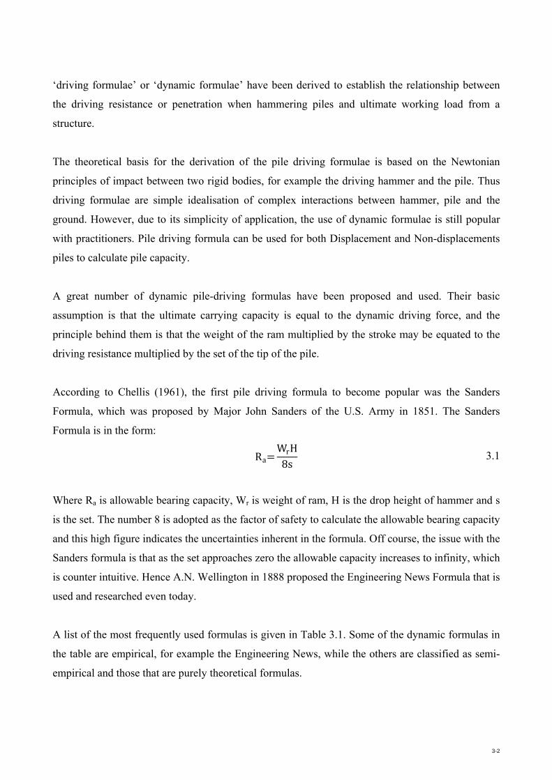
3-2
‘driving formulae’ or ‘dynamic formulae’ have been derived to establish the relationship between
the driving resistance or penetration when hammering piles and ultimate working load from a
structure.
The theoretical basis for the derivation of the pile driving formulae is based on the Newtonian
principles of impact between two rigid bodies, for example the driving hammer and the pile. Thus
driving formulae are simple idealisation of complex interactions between hammer, pile and the
ground. However, due to its simplicity of application, the use of dynamic formulae is still popular
with practitioners. Pile driving formula can be used for both Displacement and Non-displacements
piles to calculate pile capacity.
A great number of dynamic pile-driving formulas have been proposed and used. Their basic
assumption is that the ultimate carrying capacity is equal to the dynamic driving force, and the
principle behind them is that the weight of the ram multiplied by the stroke may be equated to the
driving resistance multiplied by the set of the tip of the pile.
According to Chellis (1961), the first pile driving formula to become popular was the Sanders
Formula, which was proposed by Major John Sanders of the U.S. Army in 1851. The Sanders
Formula is in the form:
Ra= WrH8s 3.1
Where Ra is allowable bearing capacity, Wr is weight of ram, H is the drop height of hammer and s
is the set. The number 8 is adopted as the factor of safety to calculate the allowable bearing capacity
and this high figure indicates the uncertainties inherent in the formula. Off course, the issue with the
Sanders formula is that as the set approaches zero the allowable capacity increases to infinity, which
is counter intuitive. Hence A.N. Wellington in 1888 proposed the Engineering News Formula that is
used and researched even today.
A list of the most frequently used formulas is given in Table 3.1. Some of the dynamic formulas in
the table are empirical, for example the Engineering News, while the others are classified as semi-
empirical and those that are purely theoretical formulas.

3-3
As it can be noted that some formula assume that the penetration of the pile is linearly proportional
to the ram energy, some uses the square root of the ram energy (Gates formula) and some cube root
of the stroke or energy.
The underlying theory of the pile dynamic formulas is based on assuming instant propagation of
force through the pile, whereas according to the solution of the one-dimensional wave equation, the
force actually travels in a wave. The amount of pile skin friction and proportion of plastic to elastic
yield of the soil have a great effect on these waves.
Currently, apart from the driving formula, there are two other methods that are used to measure pile
performance very accurately: Pile Load Testing (Static, Statnamic) and Pile Dynamic Analysis
(PDA) using computer signal matching analysis software CAPWAP. However, the limitations of
both of these tests are the high cost involved. In any given project only a very limited percentage (
0.5% to 1.0% ) of piles are tested by static load testing and 5% to 10% of piles are tested by PDA
test and signal matching analysis.
One of the main sources of error in the application of dynamic formula is the determination of the
actual energy delivered to piles. Longitudinal studies of PDA testing for large projects demonstrate
that during a contract energy delivered can vary up to 30% or more, hence this is a substantial and
underlying error in driving formula unless the energy can be established for each pile.
New equipments, such as the IBIS-S radar, provide an opportunity to compute or infer the true
hammer energy delivered to each contract pile and also measure the pile penetration (set and
temporary compression). By virtue of this method, accurate input into pile driving formula,
especially Hiley Formula, is possible:

3-4
Table 3.1 List of most commonly used dynamic formula (after Fragaszy et al., 1988)

3-5
The energy delivered by hammer depends on mainly the mass and velocity of the hammer at impact
which is difficult to measure. The energy transferred from the pile to the hammer is the ratio of the
actual energy transferred to the pile and the theoretical energy (W×H).
Other dynamic formulas studied for comparison reasons were the Gates and MnDOT formula.
Gates (1957) first proposed the empirical formula. The Mn/DOT formula was developed by
Paikowsky et al. (2009) as a result of a research project supported by Minnesota Department of
Transport and Minnesota State University.
In the literature, three major shortcomings of the energy or dynamic method are the uncertainty of
the actual hammer energy input to the pile top, as well as the measurement of pile penetration.
Traditionally the hammer energy was assumed constant and the ‘set’ measurements were not really
accurate. Figure 2.17 depicts the set-card method used to evaluate the set and quake values. Also,
the dynamic formulas do not take dynamic resistance into account and hence the capacity must be
factored for the dynamic component. The magnitude of this factor is thought to be a function of
resistance weighed pile velocity. With the IBIS-S radar it is now possible to record the set (S) and
temporary compression (C) much more accurately and thus can greatly improve the results from the
dynamic formulas.
Lim and Broms (1990) concluded that unless the energy delivered by the hammer is constant
(which has been shown to be not the case), the set used in Equation 2.5 and Equation 2.6 cannot be
used in defining pile performance.
The well-known dynamic formulas have been criticised in some publications. The reliability of the
dynamic formulas is well characterised in publication by Hannigan et al.(1998), in which it was
concluded that "... pile capacities determined from dynamic formulas have shown poor correlations
and wide scatter when statistically compared with static load test result”. However, Hannigan et al.
(1998) ignores the fact that this poor performance is due to the fact that the static tests are often
carried out days after the initial driving event. Thus the time dependency of pile capacity, discussed
in later sections, is often ignored.
Others such as Hussein et al. (1995), Rausche et al. (1997), Hannigan et al. (1998), and Svinkin
(2002) provide detailed discussion of the deficiencies of the dynamic formula and its comparison

3-6
with the dynamic and static testings. Rausche et al. (1997) in a research project supported by
FHWA compiled a database of static analysis method, refined wave equations and PDA
measurement method coupled with CAPWAP pile capacity analysis. A reliability of the various
capacity prediction methods were compared with the results of static testing. The results of the
dynamic formula evaluation showed that, overall, the performance of the dynamic formula was
comparable to the other methods. The results presented show that the mean value of the capacity
prediction ratio to static by Gates formula were 0.96 (coefficient of variation=0.41) for end-of-drive
and 1.33 (coefficient of variation=0.48) for restrike compared to CAPWAP with a mean value of
0.92 (coefficient of variation =0.22) for restrike condition.
Chellis (1951, 1961) suggests that if it can be determined that the dynamic formula results are in
reasonable agreement with the wave equation analysis results, then it is permissible to use such
simple formula to be quickly applied in the field.
Lowery et al. (1968) presented the results of a study in which it was demonstrated that it was
possible to find a range between the Wave Equation Analysis and the Gates formula in which they
can be in close agreement.
Tavenas et al. (1972) presented statistical analysis drawn from approximately 478 driving records.
Based on a very large foundation built in a homogenous sand deposit it was shown in the paper that
the poor quality of the pile driving formulas originates essentially in the estimate of the driving
energy. Tavenas et al. (1976) concluded that if the energy estimation is erroneous, then in fact the
dynamic formula will also be erroneous.
Paikowsky et al. (1992, 2004) has shown that the reliability of the dynamic formulas can be
improved and in fact can be comparable to the stress wave theory calculation. Paikowsky (2004)
studied the relationship between the pile resistances to pile penetration with comparison to the pile
capacity measured from the static load tests. Based on a large database of tests, the mean values of
the ratio of static test capacity to the energy based method at the end of driving (EOD) varied
between 1.1 and 1.31.
Paikowsky (2009) carried out analysis, supported by Minnesota Department of Transport, to study
relevant case histories in a database (PD/LT2000). Paikowsky (2009) studied four dynamic

3-7
equations and based on the analysis of the PD/LT2000 database proposed a new dynamic equation
as is indicated in Table 3.2.
Table 3.2 Pile driving formulas investigated and new Mn/DOT formula proposed by Paikowsky (2009)
Paikowsky (2009) calculated capacities by these equations in Table 3.2 and performed a load
resistance calibration based statistical analysis methods. As result of this research a new equation
called Mn/DOT pile driving formula with much better performance was developed.
Zhang et al (2005) proposed a procedure that is based on direct field measurement carried out with
measurement device on-board the modern hydraulic piling rigs. The soil resistance are calculated
using kinetic and effective energies over 1m of penetration and it is shown that the energy indicator
compare well with the measures static load tests.
Current research in the area includes the probabilistic method applied to the energy approach, Liang
et al. (1997), in which the authors introduce the Smith pile-soil model and treats the shaft and toe

3-8
resistances separately. However, the results are widely scattered. Sakai et al (1996) and Uto et al.
(1981, 1992) derived an approximate dynamic formula based on the stress-wave theory.
Triantafyllidis (2001) modified Hiley formula, also based on the stress-wave theory, to be used for
very long piles driven into weathered mudstone. The interesting aspect of the results is that when
viscosity or damping parameter was allowed for, the comparison between Hiley and the static
loading result using H-pile matched very well. This is precisely one of the main focuses of the
current research by the author.
3.3 Analysis of Energy Losses
The dynamic formulas as well as the more advanced wave-equation analysis all take the energy
losses in the driving system, pile and the soil into account to render them reliable.
A typical theoretical analysis of the energy losses together with the formulas for use in various
cases is shown in Table 3.3 below. Chellis (1951) provides a good analysis of hammer impact
energy and it losses in pile driving process and tries to develop equations to account for the energy
losses as a result. In a practical sense, the energy loses can be further simplified and even easily
measured with accurate instrumentation as it is described in the subsequent sections.
Table 3.3 Typical analysis of driving formula to include energy losses (Chellis 1951)
The efficiency of the driving system is the net energy available to drive a pile. Energy is wasted by
friction in the ram, bruising the pile, by the elastic rebound of the hammer and pile, by producing

3-9
vibrations and by generating heat. It has been shown in this research that the higher the velocity of
ram at impact, the greater the energy loss. Therefore, heavy rams with low drop give higher
efficiency than light rams with a high drop. This explains in part the superior efficiency of the
hydraulic hammer as well as having rapid succession of blows or high blow counts.
Hölscher et al (1996) and Hajduk et al (2000) have shown that in low driving resistance (easy
driving), high acceleration and velocity develop at the tip and in the high resistance case (hard
driving), there is small acceleration at the tip, resulting very small mobilisation of the soil mass
hence the corresponding energy loss due to soil motion is small.
It has been known that the reason for the discrepancy of the pile driving formulae is that the
dynamic formulae do not take dynamic resistance into account and hence the capacity must be
factored for the dynamic component. The other reason for the poor reputation of the dynamic
formula comes from the variation in hammer performance which have not been detected and also
from the time-dependant variations in the pile capacity i.e. comparing end-of-drive capacity with
test capacity days, weeks or months later. Without special very accurate measurements, the actual
energy delivered to the pile must be estimated from an assumed hammer efficiency and a
coefficient of restitution which may be assumed from text books, but can never be known or
measured on a project-specific basis.
3.4 Performance Comparison of Dynamic Formulas
Years of correlations between dynamic piles testing the driving formulas have shown that there is a
strong relationship between the dynamic testing and the dynamic formulas. Several studies by
Olsen (1967), Long (2002) and Tavenas (1972) have been carried out to determine and compare the
performance of the dynamic formulas with the higher order pile testing methods.
Olsen (1967) showed that the predicted accuracy is poor and to minimise risk, large safety factors
are necessary. However, a more recent study by Long (2002) has shown that the accuracy can be
improved and in fact can be as accurate as the Stress-Wave theory calculation.
McVay and Kuo (2000) undertook a comparative study on a database of 247 piles for both EOD
and BOR conditions based on the LRFD design, for example, load resistance factor and reliability

3-10
factor. The study investigated and compared eight dynamic methods as shown in Table 3.4 below.
The study suggested a factor of safety (FOS) of 1 for the FDOT formula, FOS of 3 for Gates and
FOS of 2.5 for the PDA Case and CAPWAP methods. These results are highly interesting, as they
indicate that the dynamic formula can be improved to match or even perform better than the higher-
order wave equation analysis methods.
Table 3.4 Safety factors for dynamic methods (after McVay and Kuo 2000)
Dynamic test method Equation Suggested FOS
ENR formula Ru= Wrh (s+0.1)⁄ 6
Modified ENR
formula
Ru= (1.25ehEh)(Wr+e2Wp) (s+0.1) Wr+Wp 6
Gates formula Ru=27 ehEh(1-logs) 3
FDOT formula Ru= 2Eh (s+0.1+0.01Wp)⁄ 1
Paikowsky method Ru= Emax (s+ (Dmax-s) 2⁄ )⁄ -
Sakai method Ru=(AE L⁄ ) Wp 2Wr⁄ (Dmax-s) 2.5
PDA Case method Ru=0.5(1-Jc)(P1+Zv1)+0.5(1+Jc)(P2-Zv2) 2.5
CAPWAP method CAPWAP signal matching software 2.5
McVay and Kuo (2009) concluded that the CAPWAP, PDA and the energy method (Paikowsky,
1992) are approximately twice as efficient as the other dynamic formula such as Gates, FDOT and
ENR. McVay asserts that the use of multiple methods, both static and dynamic, and that the
capacity evaluated by this procedure would give more reliable result than by a single method.
McVay and Kuo (2009) computed the factor of safety based on the LRFD design given in Table 3.5
below.

3-11
Table 3.5 Recommended safety factors for dynamic methods (after McVay & Kuo 2000)
Fragaszy et al. (1988) also undertook a comparative study into the reliability of ten pile driving
formula as indicated in Table 3.6. The study included 63 pile load tests and the ultimate capacities
were calculated using the elastic tangent and double tangent methods. Also a statistical analysis was
carried out on the results of the calculated capacities by the various methods, and it was concluded
that the Gates formula proved the best while the ENR performed the worst. A summary of the
results is given in Table 3.6 below.

3-12
Table 3.6 Comparison of results by Fragaszy et al. (1988)
It is interesting to note, despite the under performance of the hiley formula, that the results in both
soil types are very consistent.
Paikowsky et al. (2004) undertook a comprehensive and the largest study to develop load resistance
factors for pile foundations. It comprised collection of case histories into a database called
PD/LT2000. The database included static and dynamic analysis tests for concrete, H and tube piles
drilled and driven in clay, sand and rock materials as well as the time testing (EOD and BOR).
The main conclusions that were drawn from the PD/LT2000 database study was that the signal
matching under-predicted pile capacity, but it performed well for BOR cases. Also, it was remarked
that the energy or dynamic method gave a good prediction of capacities during driving (EOD cases)
as it can be seen from the Table 3.7 below.

3-13
Table 3.7 Performance of dynamic test methods (Paikowsky et al., 2004)
Current work and research in the area of pile dynamic formula continue to this day with the aim of
improving the existing formula and methods (Allen et al., 2005; Paikowsky et al., 2009).
3.5 Pile Capacity Variations with Time
Piles normally carry their design loads over the long life of the structure it is supporting. Therefore,
soil modification by driving and its behaviour over long time around the pile are essential with
respect to satisfactory performance of pile. During pile driving, the soil around the pile experiences
plastic deformations, remoulding and pore pressure changes. Excess pore water pressure developed
during driving reduces the effective soil shear strength and ultimate pile capacity. After the
completion of pile driving, soil reconsolidation, as result of the pore water dissipation as well as
thixotropy (Mitchell, 1960), are usually accompanied by an increase in pile capacity that is called
soil setup. The amount of increase in pile capacity depends on soil properties and pile
characteristics. In some soils such as saturated sandy and end-bearing piles in shale, the ultimate
pile capacity may decrease (soil relaxation) after the initial driving.
This phenomenon of time-dependent strength gain and loss in soils related to pile driving has been
studied and published by Davie (1991), Komurka (2003), Paikowsky et al (1996), Paikowsky et al

3-14
(2005), Skov and Denver (1998), Svinkin (1994), Tavenas (1977), Thompson (1985), Tomlinson
(2001), Yang (2009) and others. A summary of the empirical equations presenting the capacity
variation over time is given in Table 3.8.
Table 3.8 Empirical equations presenting pile capacity change over time Komurka et al (2003)
However, this gain or loss in capacity can be difficult to measure as it relies on the assumption that
a decrease in pile resistance between the EOD and BOR indicates that relaxation has occurred as
long as the same driving system is used in both cases. Such assumptions do not take into
consideration variations in the hammer performance or changes in the nature of the pile support.
Currently PDA equipment is used to measure strain and acceleration in piles during driving and use
CAPWAP analysis to estimate bearing capacity changes in piles over time. A study by Thompson
(1985) indicates that decreases in penetration resistance are more commonly the result of changes in
pile driver performance than in soil bearing capacity, and this type of capacity decrease is called
apparent relaxation. Thompson presented results of case histories from six sites and showed that in
some cases apparent relaxation was observed and only in two cases there were real relaxation that
was found to be associated with localised geotechnical conditions.

3-15
The decrease of capacity with time after driving has been observed to be associated with the use of
single-acting diesel hammers. These hammers tend to decrease in efficiency after extended hard
driving.
Paikowsky et al (1996) utilised an extensive database that included EOD, BOR, and PLT
information on variety of types and sizes of piles driven in clayey soils and it was shown that the
capacity increased with time. Paikowsky et al (2005) showed that piles driven in low permeability
soils also gained capacity over time and it was believed to be controlled by the mechanisms of
effective stress increase due to the dissipation of excess pore pressures and stress independent
phenomena such as strength increase due to thixotropy bonding as reported by Mitchell (1960).
Recently, research efforts have been made to quantify time dependent pile capacity and develop a
methodology to incorporate this time dependency of pile capacity into pile design by utilising in-
situ testing.
3.6 IBIS Radar
The IBIS radar system is recently developed non-contact equipment that measures displacement,
velocity, acceleration and vibration in civil engineering applications. It comes in two configurations
such as IBIS-L and IBIS-S. The IBIS-L configuration is used for static terrain deformation
monitoring and is mainly used in mining and slope stability applications. The IBIS-S configuration
is used for dynamic and static monitoring by remote sensing of structures such as buildings, bridges
and telecommunication towers.
The IBIS-S radar unit can simultaneously monitor several points, providing the displacement
response for each point. The unit operates at frequency of 200Hz, displacement accuracy of
0.01mm and range of up to 1km (IDS, 2008; IDS Australia, 2009). Bernardini et al. (2007)
conducted a laboratory test and it showed an excellent quality of the displacement measurements
and a good operational stability. IDS Australia (2009) performed some real validation tests with
accelerometers and LVDTs and the results showed an excellent match with the accelerometers and
LVDTs tests.

3-16
The main advantage of IBIS-S, apart from the accuracy, range and resolution, is the fact that it can
be operated in all weather conditions over very long distances without the need of accessing the
target to install sensor or optical targets. However, if required, then one or several specific points on
a target could to be measured by a simple passive radar reflector that can be easily fixed. All the
measured quantities are displayed in real time via a computer terminal as indicated in Figure 3.1.
Figure 3.1 Purpose made real-time monitoring of deformation by radar IBIS-S (IDS Australia, 2009).
It should be emphasised that because IBIS-S unit has never been used in piling application and its
use was first suggested by the author and trial test was conducted at a test site. Therefore, the
purpose built software used for the test was not well suited for the pile testing and the existing
software can be easily customised to calculate the required parameters.

3-17
A passive reflector was made at RMIT’s laboratory in the form of a V-shape and it was bolted to
the pile at approximate same vertical distance as the strain transducers and the accelerometer, as
shown in Figure 5.2. Continuous readings were taken of all the blows during the two stages.
The radar unit operates on a 12V battery and comes with a hard case. It also comes with an
adjustable tripod for easy and quick set up as shown in Figure 3.1.
IDS Australia (2009) presented the performance of IBIS-S with the results of a total station as
shown in Figure 3.2. It can be seen that the instrument’s performance is excellent and very stable.
Figure 3.2 IBIS-S measurement accuracy (IDS Australia, 2009)
Bernandini (2007) carried out a laboratory performance test in a laboratory on a mass-spring set up
as shown in Figure 3.3.

3-18
Figure 3.3 IBIS-S radar mass-spring performance test in laboratory (Bernardini, 2007)
The result of the measurement, Figure 3.4, indicates an excellent quality of the displacement
measurements and a good operating stability of the equipment. It also confirms the very good
quality of the measurements and that the displacement sensitivity of the sensor in the order of
0.01mm.
Figure 3.4 The first 60 second of the displacement-time measurement by IBIS-S (Bernardini, 2007)
The new radar system is capable of measuring the displacement response of several points of a
structure and provides a direct measurement of displacement, which is often of interest in civil
engineering applications.

4-1
Chapter 4
4 GRLWEAP Numerical Analysis
4.1 Background
As discussed in the previous chapter, the GRLWEAP program was developed by Goble & Rausche
in 1976. The first version was called WEAP and it was later updated to GRLWEAP with many
modifications and improvements. The program is founded on the Smiths (1960) solution of the
wave equation that is based on the discrete element idealisation of the hammer-soil-pile system, as
shown in Figure 4.1.

4-2
Figure 4.1 GRLWEAP pile, soil and driving system (hammer, helmet & cushion) modelling (PDI 2005)
Although, contrary to the dynamic formulas, GRLWEAP does not directly use the energy approach,
but it rather uses the concept of energy losses and energy transfer as results of the pile driving
process. The energy balance equation together with the schematic presentation of hammer, driving
system, pile and soil is given in Figure 4.2.
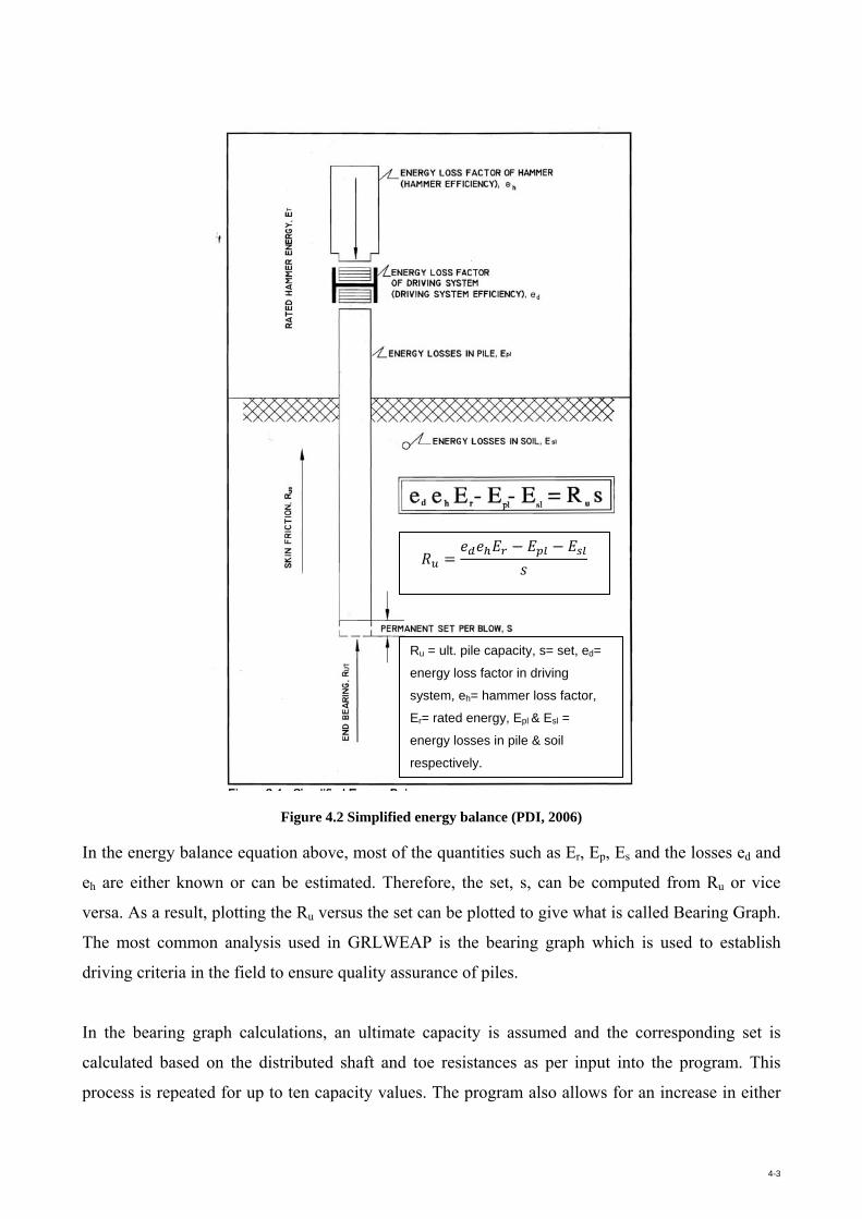
4-3
Figure 4.2 Simplified energy balance (PDI, 2006)
In the energy balance equation above, most of the quantities such as Er, Ep, Es and the losses ed and
eh are either known or can be estimated. Therefore, the set, s, can be computed from Ru or vice
versa. As a result, plotting the Ru versus the set can be plotted to give what is called Bearing Graph.
The most common analysis used in GRLWEAP is the bearing graph which is used to establish
driving criteria in the field to ensure quality assurance of piles.
In the bearing graph calculations, an ultimate capacity is assumed and the corresponding set is
calculated based on the distributed shaft and toe resistances as per input into the program. This
process is repeated for up to ten capacity values. The program also allows for an increase in either
𝑅 = 𝑒 𝑒 𝐸 − 𝐸 − 𝐸𝑠
Ru = ult. pile capacity, s= set, ed=
energy loss factor in driving
system, eh= hammer loss factor,
Er= rated energy, Epl & Esl =
energy losses in pile & soil
respectively.

4-4
shaft or toe resistances while the other resistance component is held constant for the ten capacities
that are input into the program.
Furthermore, the soil model input is also included in the code. The soil model is based on the static
formulas available in many standard geotechnical textbooks and is also briefly discussed in Section
2.5.1 of this thesis.
It must be noted that the fundamental difference between the dynamic formula and the wave
equation methods are the fact that the energy in the soil, pile and the losses are calculated
mathematically. A full detail of the GRLWEAP program background can be found in PDI (2006).
4.2 GRLWEAP Inputs
The main input data in GRLWEAP™ program are hammer, driving system (cushion) and pile
details as well as soil parameters. It outputs driving stresses, hammer performance and the pile
bearing capacity both graphically and in tabular format. Since 2002, the GRLWEAP™ has included
the Residual Stress Analysis (RSA), which is a concept relating to fact that the pile shaft is
elastically compressed during hammer strokes and that the resistance distribution between shaft and
base vary. RSA analysis is not undertaken for end bearing piles, where the toe capacity significantly
larger than the skin friction.
For the hammer, the program provides a large data file which is a compilation of basic properties of
many impact hammers, powered by air, steam, hydraulic pressure, or diesel combustion. Once the
model is setup, the program then does an analysis of the model that consists primarily of springs,
masses and dashpots.
The driving system, consisting of striker plate, cushion, helmet and pile cushion (for concrete piles)
that are represented by two non-linear springs and a mass can be entered via the program’s input
screen. Again, the standard properties of the driving system are inbuilt into the program and can be
modified if one wishes so. The cushions can be specified in the program by the area, elastic
modulus and the thickness or by the stiffness alone. Pile cushion is only entered for concrete piles
and it can be specified by the thickness and the program assumes the elastic modulus value for a

4-5
new cushion. However, this assumption may not be correct for the EOD conditions and the
program manual suggests a value of approximately 2.5 times the early driving conditions, for
example, 500 MPa instead of 200 MPa.
Pile cushions are only used for concrete piles. In the field during pile driving, the cushion properties
change over the short life of the cushion material. For example, plywood may compress to half of
its initial thickness and its elastic modulus may increase.
The hammer cushion material is usually a hard man made material and the help files of GRLWEAP
contain the manufacturers recommended values. If the cushion consists of two sandwiched
materials, then the combined properties can be calculated.
The pile cushion is a relatively soft element, usually located underneath the helmet and immediately
above the pile top. The pile cushion material is usually wood, most frequently plywood. Also
softwood or hardwood boards have been used with the grain perpendicular to the axis of the
hammer. In some countries, felt, sisal fabric, rope or other soft materials are used. In general, it is
recommended to use only materials for which engineering properties can be accurately determined.
In the analysis, the hammer’s transmitted energy to the pile determines the pile stresses. The
stiffness of the driving system, non-linearity of material and coefficient of restitution all affect the
energy transfer and hence the pile top stresses. Energy losses due to bending, poor surfaces contact,
and damaged components etcetera are not well understood.
Pile data consists of total length, cross-section area, toe area, elastic modulus and specific gravity.
Many different pile profile options that are available are non-uniform, segmental and open ended
piles. Pile mechanical splice and cracks can also be performed by entering ‘tension slack’, which
allows for the extension of the splice with zero tension force.
The coefficient of restitution for the material of the cushion as a decimal number range from 0.1 to
1.0. The cushion coefficient of restitution is a material property, which indicates the fraction of
energy that is temporarily stored in the cushion during compression that is not lost. For example, a
steel ball dropped onto a steel plate may bounce back to 100% of the drop height. It’s COR would

4-6
then be 1.0. Numerically, in GRLWEAP, a COR of 0.0 is not an acceptable input. For man-made
materials, if nothing else is known, a 0.8 value is a good estimate. For wood COR may be set to 0.5.
Although GRLWEAP performs calculation of soil static resistance in the analysis, but it is only an
estimate and the value calculated is found by the author to be non-consistent. So for the bearing
graph analysis, a separate static analysis program called DRIVEN (see Appendix D) was used to
evaluate the static shaft and toe resistances. Although the pile’s ultimate capacity is changed, but
the skin and toe resistance distribution is maintained constant throughout the analysis. Another
words, as the driving process continue, it is not necessary to recalculate the quake, damping
parameters and the skin and toe resistance distribution.
As mentioned earlier, in the GRLWEAP code, two simple static analysis methods are included. One
is based on Soil Type (ST) and the other is SPT N-value based (SA) methods. In this research
endeavour, only the ST method was used. However, these two methods of pile capacity
determination are not very accurate. Therefore, another program called DRIVEN (see Appendix D)
was used to calculate the shaft and toe resistances and the values were plugged in the GRLWEAP
program.
The ST method is intended for both Driveability and Bearing Graph analyses. It uses the β-Method
(static geotechnical capacity as briefly mentioned Section 2.5.1) to calculate the shaft and toe
resistance and, hence, the percentage of shaft and toe distribution.
4.3 Analysis Method
The basic result of a wave equation analysis is the bearing graph which relates bearing capacity to
blow count for a particular pile depth. In this analysis, an ultimate capacity is assumed then it is
distributed along the shaft as per input and the set or blow count is calculated for this ultimate
capacity. A higher capacity is selected and it is distributed along the shaft and toe and the again the
set is calculated followed by dynamic analysis. GRLWEAP analyses up to ten ultimate capacities
and then is plotted against sets or blow counts.

4-7
To undertake a GRLWEAP parametric analysis, it was considered to study the effect of different
pile-hammer and soil combinations. A summary of the cases that were studied is shown in Table 4.1
below.
Table 4.1 A summary of hammer, pile and soil type combinations in the study
As it can be seen, numerical simulations were carried out using most common hammers such as
Delmag, Junttan and MKT together with three rated energies at approximately 3, 5 and 10 tonnes.
Also for each hammer three different drop heights of 0.25m, 0.5m and 1m were adopted to produce
a wide range of energies and capacities, as shown in Table 4.2.
Table 4.2 Hammer Details
Hammer Model Ram
Weight(kN)
Max.
Stroke(m)
Rated
Energy(kNm)
Delmag
D15 29.43 1.2 35.32
D19-42 49.10 1.2 58.86
D36-13 98.10 1.2 117.72
Junttan
HHK3 14.69 2.5 36.75
HHK5 17.8 3.3 58.65
HHK10 35.29 3.22 113.69
MKT
S-8 35.60 1.0 35.27
MS500 48.95 1.2 59.68
S-20 89.00 1.0 81.38
Hammer Hammer Pile Soil Stroke TotalType Weight Type Type
-350mm Sq Precast
3 3 2 36 3 1944
Delmag Junttan
MKT -327mm (12.7mm thick) Sq Precast
1m, 0.5m, 0.25m
3T 5T
10TS
oil c
ombi
natio
ns a
s in
Tab
le 4
.5
Tot
al n
umbe
r of
cas
es
anal
ysed
in G
RLW
EA
P
Tube

4-8
In the case of diesel hammers, the percentages of the maximum hammer strokes were selected. As
a result, this systematic analysis produced a total of 1944 cases representing all possible
combinations of hammer, pile and soil types, as well as different hammer strokes. After the
analysis, the data were sifted through and collated to produce about 20,000 rows by 35 columns of
Excel data sheet. A sample of the spreadsheet data sets is shown in Table 4.4. The hammer and pile
cushion details that were used in the GRLWEAP analysis are presented in Table 4.3.

4-9
Table 4.3 Hammer and Pile Cushion Details
Concrete pile Steel pile
Delmag Junttan MKT Delmag Junttan MKT
Hammer Cushion
Pile Cushion
Hammer Cushion HHK10
Pile Cushion
Hammer Cushion
Pile Cushion
Hammer Cushion
Hammer Cushion HHK10
Hammer Cushion
Material Nylon Plywood Alum/
Conbest Alum/
Conbest Plywood
Alum/ Conbest
Plywood Nylon Alum/
Conbest Alum/
Conbest Alum/
Conbest
Area (cm2) 1465.5 1225 1590.3 4418.1 1225 - 1225 1464.5 1590.3 4418.1 -
Elastic Mod.(MPa) 3654.2 207 2500 2500 207 - 207 3654.2 2500 2500 -
Thickness(mm) 50.8 94 200 210 94 - 94 50.8 200 210 -
COR 0.8 0.5 0.9 0.9 0.5 0.8 0.5 0.8 0.9 0.9 0.8
Stiffness(kN/mm) 10534.6 269.8 1987.9 5259.6 269.8 6329 269.8 10534.6 1987.9 5259.6 6329
Table 4.4 Sample of the database from GRLWEAP analysis
Hammer Type Model Ram Weight (kN) Rate Energy (kJ) Potential Energy(kJ) Kinetic Energy (kJ) Impact Vel. (m/s) Pile Type Soil Type Rut (kN) Bl Ct (b/m) Stroke Ten Str (Mpa) i t(ms) CompStr i t(ms) ENTHRU (kJ) No mxTForce t mxCForce t mxTStrss t mxCStrss t maxV t maxD t maxEt Set(mm) Hiley(kN) HCF(-)JUNTTAN HHK 29.43 35.32 29.43 23.54 3.96 350 Precst vl-vl 250 23.8 1 -2.45 4 12 14.72 2 7 14.1 1 0 0 1802 7 0 0 14.7 7 2.64 9 45.5 40 14.1 42.01681 322.2238 1.2888953JUNTTAN HHK 29.43 35.32 29.43 23.54 3.96 350 Precst vl-vl 500 52.2 1 -1.75 3 15 14.94 2 7 14 1 0 0 1817 7 0 0 14.8 7 2.33 9 23.1 22 13.99 19.15709 662.1374 1.3242749JUNTTAN HHK 29.43 35.32 29.43 23.54 3.96 350 Precst vl-vl 750 81.3 1 -1.4 3 15 15.15 2 7 14.1 1 0 0 1831 7 0 0 14.9 7 2.05 9 16.4 16 14.07 12.30012 980.4836 1.3073115JUNTTAN HHK 29.43 35.32 29.43 23.54 3.96 350 Precst vl-vl 1000 109.9 1 -1.5 8 25 15.36 2 7 14.2 1 0 0 1845 7 0 0 15.1 7 1.81 9 13.3 16 14.2 9.099181 1267.903 1.2679035JUNTTAN HHK 29.43 35.32 29.43 23.54 3.96 350 Precst vl-vl 1500 188.9 1 -3.03 5 23 15.76 2 7 13.2 1 0 0 1874 7 0 0 15.3 7 1.44 4 9.8 13 13.23 5.293806 1753.037 1.1686913JUNTTAN HHK 29.43 35.32 29.43 23.54 3.96 350 Precst vl-vl 2000 393.4 1 -2.16 5 21 16.16 2 7 12.1 1 0 0 1903 7 0 0 15.5 7 1.44 4 8.4 10 12.14 2.541942 2218.985 1.1094923JUNTTAN HHK 29.43 35.32 29.43 23.54 3.96 350 Precst vl-vl 2500 1278.5 1 -2.3 4 21 17.12 4 10 11.2 1 0 0 1931 7 0 0 15.8 7 1.43 4 7.5 10 11.18 0.782167 2699.777 1.0799107JUNTTAN HHK 29.43 35.32 29.43 23.54 3.96 350 Precst vl-vl 3000 9999 1 -3.31 4 18 18.74 4 10 10.4 1 0 0 1959 7 0 0 16 7 1.43 4 6.9 10 10.35 0.10001 2957.139 0.9857129JUNTTAN HHK 29.43 35.32 7.3575 5.89 1.98 350 Precst vl-vl 250 77.7 0.25 -0.89 5 13 7.35 1 8 4 1 0 0 900 8 0 0 7.3 8 1.23 10 16.4 28 3.97 12.87001 271.2674 1.0850696JUNTTAN HHK 29.43 35.32 7.3575 5.89 1.98 350 Precst vl-vl 500 186.3 0.25 -0.75 6 30 7.43 1 8 4 1 0 0 911 8 0 0 7.4 8 1.03 10 9 17 3.97 5.367687 552.629 1.105258JUNTTAN HHK 29.43 35.32 7.3575 5.89 1.98 350 Precst vl-vl 750 344.8 0.25 -0.75 5 26 7.52 1 8 3.9 1 0 0 921 8 0 0 7.5 8 0.89 9 6.8 15 3.88 2.900232 799.9809 1.0666412JUNTTAN HHK 29.43 35.32 7.3575 5.89 1.98 350 Precst vl-vl 1000 682.3 0.25 -1.96 6 24 7.6 1 8 3.6 1 0 0 932 8 0 0 7.6 8 0.8 8 5.5 11 3.6 1.465631 1033.646 1.0336465JUNTTAN HHK 29.43 35.32 7.3575 5.89 1.98 350 Precst vl-vl 1166.9 1389.3 0.25 -1.93 6 24 7.66 1 8 3.5 1 0 0 952 8 0 0 7.8 8 0.71 4 4.6 11 3.27 0.719787 1229.373 1.0535372JUNTTAN HHK 29.43 35.32 7.3575 5.89 1.98 350 Precst vl-vl 1500 9999 0.25 -1.18 0 0 8.49 0 0 3.3 1 0 0 939 8 0 0 7.7 8 0.76 8 5.1 11 3.49 0.10001 1342.305 0.8948701JUNTTAN HHK 29.43 35.32 14.715 11.77 2.80 350 Precst vl-vl 250 42.1 0.5 -1.43 4 12 10.46 1 7 7.5 1 0 0 1281 7 0 0 10.5 7 1.79 10 27.2 34 7.45 23.75297 292.4265 1.1697061JUNTTAN HHK 29.43 35.32 14.715 11.77 2.80 350 Precst vl-vl 500 94.2 0.5 -0.53 4 36 10.56 1 7 7.4 1 0 0 1293 7 0 0 10.6 7 1.53 9 14.1 19 7.41 10.61571 599.6186 1.1992372JUNTTAN HHK 29.43 35.32 14.715 11.77 2.80 350 Precst vl-vl 750 154.8 0.5 -0.63 5 27 10.66 1 7 7.4 1 0 0 1306 7 0 0 10.7 7 1.3 9 10.3 16 7.42 6.459948 885.4443 1.1805923JUNTTAN HHK 29.43 35.32 14.715 11.77 2.80 350 Precst vl-vl 1000 227.9 0.5 -1.76 6 24 10.81 2 7 7.2 1 0 0 1318 7 0 0 10.8 7 1.11 9 8.4 14 7.2 4.387889 1126.065 1.1260654JUNTTAN HHK 29.43 35.32 14.715 11.77 2.80 350 Precst vl-vl 1500 627.7 0.5 -2.14 5 23 11.15 2 7 6.5 1 0 0 1343 7 0 0 11 7 1.02 4 6.5 11 6.47 1.593118 1598.889 1.0659263

4-10
The soil types and their consistencies were also based on the parameters given in the GRLWEAP
program and range of cohesive and non-cohesive soils with various consistencies were selected. A
summary of the soil combination as well as the standard soil profile is shown in Table 4.5.
Table 4.5 Soil combinations and cross-section profiles used in the GRLWEAP analysis
The standard GRLWEAP soil resistance parameters, toe quake value (dependent on the pile toe
diameter) and shaft and toe quake damping are shown in Table 4.6 below.
Table 4.6 GRLWEAP resistance parameters for ST analysis for cohesion-less soils
Soil Type SPT N Friction angle Unit Weight β Nt Rs Rt
Deg. kN/m3 Limit (kPa)
Very loose 2 25-30 13.5 0.203 12.1 24 2400
Loose 7 27-32 16 0.242 18.1 48 4800
Medium 20 30-35 18.5 0.313 33.2 72 7200
Dense 40 35-40 19.5 0.483 86.0 96 9600
Very Dense 50+ 38-43 22 0.627 147.0 192 19000
10m
VL = very loose
MD = med. dense
VD = very dense
Cross-section

4-11
For cohesive soils, GRLWEAP adopts α-method, also called total stress method, for the ST
analysis. For non-cohesive the methods relies on the unconfined compressive strength of soil. The
unconfined compressive strength (qu), the shaft and bearing soil resistance as a function of soil type
for cohesive soils are given in Table 4.7.
Table 4.7 GRLWEAP resistance parameters for cohesive soils
Soil Type SPT N qu Unit Weight Rs Rt
kPa kN/m3 kPa
Very soft 1 12 17.5 3.5 54
Soft 3 36 16 10.5 162
Medium 6 72 18.5 19 324
Stiff 12 144 19.5 38.5 648
Very stiff 24 288 22 63.5 1296
Hard 32+ 384+ 77 1728
In the GRLWEAP analysis, shaft and toe quakes and damping are the four Smith soil model
parameters that are used to model the soil dynamic behaviour. The program standard quake and
damping parameters are given in the Table 4.8. It may be noted that no quake or damping values are
given by GRLWEAP program for vibratory hammers because of the complex nature of such
hammers and the lack of testing experience.
Table 4.8 GRLWEAP recommended Quake values for driven piles
Soil Type Pile Type Quake (mm)
Shaft Quake All soil types All types 2.5
Toe Quake
All soil types, soft rock Non-displacement piles* 2.5
Very dense & Hard soils Displacement piles **of diameter or width D D/120
Loose or soft soils Displacement piles *of diameter or width D D/60
Hard rock All types 1.0
*= Non-displacement piles are sheet piles, H-piles or open ended unplugged piles
**= Displacement piles are all other piles including closed-end tube and solid concrete piles

4-12
Also, the recommended damping values suggested by GRLWEAP is summarised in Table 4.9 and
in general, the Smith damping is used unless the residual stress analysis (briefly discussed in
Section 4.2) is required and in which case the Smith Viscous soil damping is used.
Table 4.9 GRLWEAP recommended damping values for driven piles
Soil Type Damping Factor (s/m)
Shaft damping Non-cohesive soils * 0.16
Toe damping Cohesive soils** 0.65
All soil types 0.5
*= Non-cohesive soils are sand type soils, **= Cohesive soils are clay type soils
For all the analysis in GRLWEAP, the recommended quake and damping values given in the above
Table 4.8 and Table 4.9 were used in this research.
As discussed previously, for the skin and toe resistance, a static analysis program called DRIVEN
was used to calculate the shaft and toe resistance ratios. In order to make the analysis consistent, the
GRLWEAP resistance parameters for cohesive and non-cohesive soils were adopted and used in
DRIVEN program. Table 4.10 shows a summary of the parameters used in the DRIVEN program.
Table 4.10 Input parameters in DRIVEN
After utilisation of the parameters in DRIVEN, the results were tabulated in total skin/shaft and toe
resistance and the ratios for the two pile types were calculated in excel spreadsheet, as shown in
Soil Type SPT(N) Unit Weight Cu Friction angleno. kN/m^3 kPa degree
Soft 3 17.5 20 -Stiff 12 20.5 75 -Hard 32 22 200 -Very Loose 2 13.5 - 25Medium 20 18.5 - 30Very Dense 50 22 - 40

4-13
Table 4.11 and Table 4.12, and the results of the DRIVEN program were back-substituted into
GRLWEAP for the shaft and toe resistance distribution.

4-14
Table 4.11 DRIVEN output of skin and end bearing capacities for precast concrete pile
Table 4.12 DRIVEN output of skin and end bearing capacities for tube pile
350mm Precast Concrete Pile
ρ(kN/m^3)Cu/φ (kPa/deg)
Shaft(kN) Tip(kN) Total Shaft(kN) Tip(kN) Total Shaft(kN) Tip(kN) Total Shaft(kN) Tip(kN) Total Shaft(kN) Tip(kN) Total Shaft(kN) Tip(kN) Total
234.78 22.05 256.83 234.97 82.68 317.65 235.19 220.5 455.69 235.36 78.12 313.48 235.8 78.12 313.92 238.48 2449.24 2687.791% 9% 74% 26% 52% 48% 75% 25% 75% 25% 9% 91%
964.4 22.05 986.45 965.46 82.68 1048.1 965.27 220.5 1185.8 965.35 78.12 1043.5 965.86 78.12 1044 969.01 2449.24 3418.398% 2% 92% 8% 81% 19% 93% 7% 93% 7% 28% 72%
775.27 22.05 797.32 775.95 82.68 858.63 775.76 220.5 996.26 773.87 78.12 851.99 776.45 78.12 854.57 779.83 2449.24 3229.197% 3% 90% 10% 78% 22% 91% 9% 91% 9% 24% 76%
281.71 22.05 303.76 282.39 82.68 365.07 282.2 220.49 502.69 281.99 78.12 360.11 280.86 78.12 358.98 284.4 1987.73 2272.193% 7% 77% 23% 56% 44% 78% 22% 78% 22% 13% 87%
618.38 22.05 640.43 619.07 82.68 701.75 618.88 220.49 839.37 618.87 78.12 696.99 619.34 78.12 697.46 622.18 2449.24 3071.497% 3% 88% 12% 74% 26% 89% 11% 89% 11% 20% 80%
2421.9 22.05 2444 2422.58 82.68 2505.3 2422.4 220.49 2642.9 2422.54 78.12 2500.7 2423.1 78.12 2501.2 2426.47 2449.24 4875.799% 1% 97% 3% 92% 8% 97% 3% 97% 3% 50% 50%
Top Layer CLAY
SAND
75
MD
VD
Soft
Stiff
Hard
VL
20 200 25 30 4020.5 22 13.5 18.5 2217.5
Bottom LayerCLAY SANDStiff Hard VL MD VDSoft
[email protected] Steel Tube Pile (Closed)
ρ(kN/m^3)Cu/φ (kPa/deg)
Shaft(kN) Tip(kN) Total Shaft(kN) Tip(kN) Total Shaft(kN) Tip(kN) Total Shaft(kN) Tip(kN) Total Shaft(kN) Tip(kN) Total Shaft(kN) Tip(kN) Total
193.4 15.12 208.52 193.83 56.69 250.52 193.75 151.16 344.91 193.57 53.56 247.13 193.76 53.56 247.32 194.82 1679.1 1873.9293% 7% 77% 23% 56% 44% 78% 22% 78% 22% 10% 90%
616.25 15.12 631.37 616.67 56.69 673.36 616.6 151.16 767.76 616.48 53.56 670.04 616.71 53.56 670.27 617.95 1679.1 2297.0598% 2% 92% 8% 80% 20% 92% 8% 92% 8% 27% 73%
544.26 15.12 559.38 544.68 56.69 601.37 544.61 151.16 695.77 544.51 53.56 598.07 544.76 53.56 598.32 546.1 1679.11 2225.2197% 3% 91% 9% 78% 22% 91% 9% 91% 9% 25% 75%
138.4 15.12 153.52 138.82 56.69 195.51 138.75 151.16 289.91 138.48 53.56 192.04 138.63 53.56 192.19 139.45 1362.72 1502.1790% 10% 71% 29% 48% 52% 72% 28% 72% 28% 9% 91%
292.11 15.12 307.23 292.53 56.69 349.22 292.46 151.16 443.62 292.3 53.56 345.86 292.5 53.56 346.06 293.62 1679.11 1972.7395% 5% 84% 16% 66% 34% 85% 15% 85% 15% 15% 85%
1012.86 15.12 1027.98 1013.28 56.69 1069.97 1013.21 151.16 1164.37 1013.11 53.56 1066.67 1013.36 53.56 1066.92 1014.69 1679.11 2693.899% 1% 95% 5% 87% 13% 95% 5% 95% 5% 38% 62%
VL
MD
VD
40
Top Layer
CLAY
Soft
Stiff
Hard
20 75 200 25 30
SAND
17.5
Bottom LayerCLAY SAND
Soft Stiff Hard VL MD VD20.5 22 13.5 18.5 22

4-15
As stated earlier, a total 1944 cases were analysed in GRLWEAP and only the relevant results from
an extensive data outputs were collated in a spreadsheet for further analysis. GRLWEAP is capable
of producing results both in graphical and tabular data formats. The Figure 4.3 below shows a
typical graphical output.
Figure 4.3 GRLWEAP graphical output of results
4.4 Results and Discussions
The results of the GRLWEAP numerical simulations were collated in a spreadsheet and analysed
for the following:
1. Three hammer types: Delmag, Junttan and MKT. Within each type, three different ram
weights were analysed.
2. Two different piles: Precast concrete and steel tube pile with similar effective sizes.
3. For each hammer type and ram weight, three drop heights were analysed.
4. Three soil resistance models with consistencies of soft, stiff and hard were used for the
cohesive soils, and three (very loose, medium dense & very dense) for non-cohesive soils
were used.

4-16
The results of the GRLWEAP simulations were exported and collated into a spreadsheet for further
analysis. The results of the GRLWEAP simulation analysis are shown in Appendix E. The graphs
were produced from the calculated Hiley capacities and GRLWEAP capacity ratios versus the set.
4.4.1 Delmag Hammers
Delmag diesel hammers seem to perform very well in driving concrete and steel piles. The
maximum hammer energies for the three rams with the weights of three, five and ten tonnes falling
from 0.25m, 0.5m and 1m were plotted against maximum ram velocity. As it can be seen from
Figure 4.4 and Figure 4.5, that there is reasonable correlation between the maximum energy and the
ram impact velocity. Generally, there seems to exceptionally good correlation for low hammer
energies than higher energies.
Figure 4.4 Maximum energy versus velocity for Delmag hammer - concrete pile
On the other hand, performance of the Delmag for steel pile is unusual for low Ru capacities and
relatively high set values calculated for GRLWEAP. This seems to be a bit of contradiction where
y = -2.0297x3 + 7.7641x2 - 0.1471x
y = -0.7753x3 + 5.9763x2 + 0.697x
y = -3.0388x3 + 15.811x2 - 1.6702x
0
10
20
30
40
50
60
70
0 0.5 1 1.5 2 2.5 3 3.5 4
max
E(kN
m)
maxV(m/s)
Max. Energy vs Max. Velocity for Delmag Hammers-precast pile
Delmag 3t
Delmag 5t
Delmag 10t
Poly. (Delmag 3t)
Poly. (Delmag 5t)
Poly. (Delmag 10t)
Stroke=50%
of max stroke
Stroke=100%
of max stroke
- 350mm sq.

4-17
the energy-velocity data seems to reflect which give that there is a minimum energy at the specific
set value. It could not be established how this could be possible in the real practical sense.
It should be born in mind that the pile performance in this case is not efficiencies, but rather the
implicit relationship between the ram velocity and delivered energy. This relationship is important
in the field where once ram velocity can be established and the ram energy can be inferred by the
relationship that would make it possible to use the dynamic formulas with greater confidence.
Figure 4.5 Maximum energy versus velocity for Delmag hammer - tube pile
4.4.2 Junttan Hammers
Junttan hammers perform similar to the Delmag hammers for steel piles, but its performance is
relatively poor for the precast piles as the data is widely scattered and no clear trend can be
y = 0.7655x2 + 1.1713x
y = 0.802x2 + 1.3766x
y = 0.9768x2 + 1.1058x
0
10
20
30
40
50
60
70
0 1 2 3 4 5 6 7 8
max
E(kN
m)
maxV(m/s)
Max. Energy vs Max. Velocity for Delmag hammers - tube pile
Delmag 3t
Delmag 5t
Delmag 10t
Series4
Series5
Series6
Poly. (Series4)
Poly. (Series5)
Poly. (Series6)
Stroke=50%
of max stroke
Stroke=100%
of max stroke
- 327mm tube

4-18
established. However, the velocity-energy graph in figure for the steel pile seems to indicate there is
a very good correlation and the relationship may be estimated by the given equation on the graph.
Figure 4.6 Maximum energy versus velocity for Junttan hammer - concrete pile
0
10
20
30
40
50
60
70
0 1 2 3 4 5 6
max
E(kN
m)
maxV(m/s)
Max. Energy vs Max. Velocity for Junttan Hammers - precast pile
Junttan 3t
Junttan 5t
Junttan 10t
Stroke=0.25m
Stroke=0.5m
Stroke=1m

4-19
Figure 4.7 Maximum energy versus velocity for Junttan hammer - tube pile
4.4.3 MKT Hammers
Again the energy-velocity relationship for the MKT hammers scattered and no clear correlation
exists. It should be emphasised that although there may be a relationship on a small individual case
bases, but overall, for a wide range of ground conditions, different rated energies and strokes, there
could not be a clear correlation as can be seen from Figure 4.8.
y = 2.4321x2 + 1.4548x
y = 1.6198x2 + 0.9376x
y = 1.1001x2 + 0.5198x
0
10
20
30
40
50
60
70
80
0 1 2 3 4 5 6 7 8 9
max
E(kN
m)
maxV(m/s)
Max. Energy vs Max. Velocity for Junttan hammers - tube pile
Junttan 3t
Junttan 5t
Junttan 10t
Series4
Series5
Series6
Poly. (Series4)
Poly. (Series5)
Poly. (Series6)
Stroke=0.25m
Stroke=0.5m
Stroke=1m

4-20
Figure 4.8 Maximum energy versus velocity for MKT hammer - concrete pile
MKT hammers seems to perform exceptionally well for the steel piles. Initially there is clear
relationship, as is approximated by the regression line, and then it is a horizontal line indicating that
the delivered energy cannot increase indefinitely and reaches a maximum regardless of the ram
velocity. This is shown on the Figure 4.9.
0
10
20
30
40
50
60
0 0.5 1 1.5 2 2.5 3 3.5 4 4.5 5
max
E(kN
m)
maxV(m/s)
Max. Energy vs Max. Velocity for MKT Hammers - precast pile
MKT 3t
MKT 5t
MKT 10t
Stroke=0.25m
Stroke=0.5m
Stroke=1m

4-21
Figure 4.9 Maximum energy versus velocity for MKT hammer - tube pile
4.4.4 Hiley Corrections Factor
Having analysed and established the relative performance of hammers in regards to the velocity-
energy relationship, similar analysis were carried out for establishing the hiley correction factor
(HCF) for each soil types and hammer types. Appendix E contains the results of the analyses for
each soil and hammer types. The graphs were produced by plotting the GRLWEAP and Hiley
capacity ration (or HCF) against the sets. Table 4.13 shows a summary of the range of the HCF for
the various hammers, pile types and soil conditions.
y = 2.3795x2 + 1.0755x
y = 1.3944x2 + 0.5122x
y = 1.0105x2 + 0.87x
0
10
20
30
40
50
60
70
0 1 2 3 4 5 6 7 8
max
E(kN
m)
maxV(m/s)
Max. Energy vs Max. Velocity for MKT hammers - tube pile
MKT 3t
MKT 5t
MKT 10t
Series4
Series5
Series6
Poly. (Series4)
Poly. (Series5)
Poly. (Series6)
Stroke=1m
Stroke=0.5m
Stroke=0.25

4-22
Table 4.13 Summary of range of Hiley Correction Factors for various driving system and soil types
Top Bottom HCF* Trend Top Bottom HCF TrendS-H 1.51-1.07 S-H 2.07-1.25VL-VD 1.57-1.00 VL-VD 2.03-1.13S-H 1.58-1.06 S-H 2.07-1.30VL-VD 1.59-1.02 VL-VD 2.06-1.23S-H 0.95-1.31 S-H 1.07-1.57VL-VD 0.92-1.42 VL-VD 1.08-1.72S-H 0.90-1.19 S-H 1.05-1.38VL-VD 0.90-1.32 VL-VD 1.06-1.60S-H 1.71-1.13 S-H 2.29-1.40VL-VD 1.70-1.06 VL-VD 2.26-1.26S-H 1.72-1.12 S-H 2.25-1.50VL-VD 1.71-1.00 VL-VD 2.28-1.30S-H 0.95-1.37 S-H 1.11-1.68VL-VD 0.95-1.51 VL-VD 1.12-1.88S-H 0.95-1.23 S-H 1.09-1.46VL-VD 0.95-1.39 VL-VD 1.10-1.74S-H 2.09-1.11 S-H 2.38-1.28VL-VD 2.04-1.07 VL-VD 2.26-1.19S-H 1.12-2.11 S-H 2.40-1.28VL-VD 2.09-1.09 VL-VD 2.35-1.25S-H 1.65-0.95 S-H 1.07-1.70VL-VD 0.97-1.83 VL-VD 1.09-1.74S-H 0.94-1.48 S-H 1.05-1.46VL-VD 0.94-1.68 VL-VD 1.06-1.80S-H 1.96-0.97 S-H 2.59-1.38VL-VD 1.88-0.99 VL-VD 2.53-1.19S-H 1.96-1.18 S-H 2.61-1.45VL-VD 1.96-0.93 VL-VD 2.57-1.29S-H 1.60-0.93 S-H 1.10-1.91VL-VD 0.94-1.64 VL-VD 1.07-2.05S-H 0.95-1.26 S-H 1.03-1.62VL-VD 0.92-1.47 VL-VD 1.04-1.82S-H 2.15-1.10 S-H 2.54-1.37VL-VD 2.17-0.96 VL-VD 2.50-1.13S-H 1.08-2.42 S-H 2.60-1.44VL-VD 2.25-1.02 VL-VD 2.50-1.25S-H 1.90-0.93 S-H 1.10-1.93VL-VD 0.90-1.80 VL-VD 1.05-2.14S-H 0.94-1.34 S-H 1.12-1.64VL-VD 0.90-1.60 VL-VD 1.13-1.82S-H 2.30-1.10 S-H 2.41-1.41VL-VD 2.30-1.01 VL-VD 2.35-1.15S-H 1.05-2.25 S-H 2.47-1.45VL-VD 2.13-1.18 VL-VD 2.41-1.27S-H 1.68-0.95 S-H 1.14-1.67VL-VD 1.83-0.94 VL-VD 1.07-1.99S-H 1.43-0.97 S-H 1.13-1.52VL-VD 1.70-0.95 VL-VD 1.14-1.83S-H 1.91-1.19 S-H 2.50-1.48VL-VD 1.93-1.01 VL-VD 2.44-1.15S-H 1.91-1.23 S-H 2.54-1.39VL-VD 1.85-1.10 VL-VD 2.48-1.35S-H 1.00-1.46 S-H 1.05-1.82VL-VD 1.63-0.96 VL-VD 1.14-2.04S-H 0.98-1.28 S-H 1.01-1.56VL-VD 0.98-1.48 VL-VD 1.05-1.89S-H 1.15-2.25 S-H 2.42-1.43VL-VD 2.19-1.00 VL-VD 2.39-1.14S-H 1.24-2.25 S-H 2.47-1.47VL-VD 2.25-1.06 VL-VD 2.40-1.35S-H 1.02-1.55 S-H 1.11-1.81VL-VD 1.03-1.60 VL-VD 1.13-2.03S-H 1.01-1.32 S-H 1.08-1.52VL-VD 1.56-1.02 VL-VD 1.09-1.87S-H 2.33-1.18 S-H 2.38-1.38VL-VD 2.40-1.03 VL-VD 2.32-1.13S-H 2.28-1.24 S-H 2.60-1.37VL-VD 2.31-1.05 VL-VD 2.39-1.25S-H 0.97-1.52 S-H 1.09-1.76VL-VD 0.98-1.78 VL-VD 1.04-1.98S-H 1.04-1.37 S-H 1.13-1.51VL-VD 0.97-1.53 VL-VD 1.11-1.82
*= Hiley Correction FactS= Soft, H= Hard, VL= Very Loose, VD= Very Dense
Parabolic. Nearly linear for VD soils.
Parabolic. Power for low energies.
Parabolic then linear asymptotic.
Initially steep-linear then horizontal.
Nearly constant for low hammer
energies.
Linear then assymptotic.
Power. Negative linear for low
energies.
Linear then flat. For low energies initially linear then negative
linear.
Linear then asymptotes
Linear then flat. Almost constant for
low energies. VL
VD5
to
nn
e
S
H
VL
VD
3 t
on
ne
S
H
VL
Jun
ttan
Jun
ttan
MK
TM
KT
MK
T
3 t
on
ne
De
lma
gD
elm
ag
De
lma
gJu
ntta
n
3 t
on
ne
10
to
nn
e3
to
nn
e5
to
nn
e1
0 t
on
ne
Tube Steel PilePrecast Concrete Pile
5 t
on
ne
VD
VL
H
S
10
to
nn
eS
H
VL
VD
VD
VL
H
S
3 t
on
ne
S
H
VL
VD
10
to
nn
e
S
H
VDVD
VL
H
S
5 t
on
ne
S
5 t
on
ne
S
H H
VL VL
VD VD
S
10
to
nn
e
S
H H
VL VL
VD VD
Parabolic then asymptotic.
S
3 t
on
ne
S
H H
VL VL
VD VD
Parabolic then asymptotes down.
S
5 t
on
ne
S
H H
VL VL
VD VD
S
10
to
nn
e
S
H H
VL VL
VD VD
Parabolic then asymptotes.

4-23
Overall, the HCF values are fairly uniform across the different hammers and soil types. Delmag 5t,
Junttan 3t and MKT 5t have performed really well in terms of the statistical analysis data, as shown
in Table 4.14. For the steel tube pile, Delmag 3t, Junttan 10t and MKT 5t have performed better
statistically. Also from the Table 4.14 it can be seen that the minimum and maximum range of HCF
across the table is between approximately 1.0 to 2.9 and an average of about 1.4. An interesting
point about the HFC is that generally the lower unit value is applicable for the sandy soil and the
higher value applicable for the clay soils. This indicates that for clay soils the dynamic effect is
greater due to the viscous nature of clay soils and hence the factor must be higher for clay soils. On
the other hand, for sandy soils, this dynamic effect is very small and hence the HCF approaches a
unit.
Table 4.14 Statistical analysis of HCF based on the GRLWEAP data for each hammer type
4.5 Conclusion
In this chapter, the methodology and discussion on the results of numerical analysis using
GRLWEAP has been presented.
A total of 1944 cases were analysed based on a combination of different hammer type and weight,
pile types, soil types and hammer strokes. The data were collated into a spreadsheet and further
analysis were conducted calculate and compare the range of HCF based on these variables.
Based on this study, it has been proposed that GRLWEAP analysis could be carried out to establish
the:
1. Hammer performance and efficiency;
2. Transmitted energy to piles;
3. Relationship between hammer velocity and peak energy; and
4. Set versus Resistance of piles.
Once the above have been established, the HCF can be used calculated based on these parameters.
Subsequently, the HCF can be used to evaluate pile capacity in the field with greater confidence and
reliability. In conjunction with this, radar equipment has been proposed to calculate the set and
velocity of a pile on site to make the hiley formula comparable to the wave equation techniques.
Weight 3t 5t 10t 3t 5t 10t 3t 5t 10t 3t 5t 10t 3t 5t 10t 3t 5t 10tMin. 0.947 0.897 0.941 0.864 0.831 0.861 0.959 0.926 0.887 1.032 1.016 1.046 0.992 1.013 1.069 0.919 1.052 1.010Max. 1.719 1.600 2.108 1.965 2.418 2.516 2.909 2.026 2.516 2.099 2.323 2.504 2.676 2.667 2.499 2.802 2.494 2.736Mean. 1.228 1.164 1.316 1.303 1.384 1.418 1.327 1.282 1.332 1.446 1.555 1.532 1.556 1.514 1.515 1.554 1.527 1.496STDEV 0.213 0.194 0.298 0.248 0.319 0.314 0.265 0.217 0.283 0.308 0.363 0.391 0.347 0.332 0.299 0.333 0.307 0.294
Precast Concrete PileDelmag Junttan MKTMKTJunttanDelmag
Steel Tube Pile

5-1
Chapter 5
5 FIELD STUDY
5.1 Test Site
A site located at the north-western fringe of Melbourne Central Business District (CBD) was chosen
to conduct a trial test of radar IBIS-S. The IBIS-S testing was carried out in parallel with the PDA
testing using 350mm square section precast concrete pile. The IBIS (Figure 5) was set up at an
offset distance of approximately 20m from the pile.
PDA and IBIS-S testings were carried out at the end-of-driving (EOD) under low driving resistance
(easy-driving) and high driving resistance (hard-driving) conditions. The pile was driven by a 6
tonne single-acting hydraulic (Banut) hammer with strokes of 300mm for the easy and 700mm for
hard driving conditions. The pile embedded lengths were approximately 15m and 18m for the two
pile driving conditions respectively.
5.2 Site Conditions
According to the site geotechnical report, the subsurface condition generally comprised 0.5m thick
of borrowed sedimentary rock materials (siltstone), followed by under laying Coode Island Silt
(CIS) of 10.5m thickness. The consistency of the CIS material was predominantly soft. Fishermens
Bend Silt (FBS) typically 4m in thickness, generally occur below CIS and was of stiff to very stiff
consistency. A sedimentary formation deposit called Moray Street Gravels (MSG) that mainly

5-2
comprise fine grain sandy materials, underlay the FBS formation. The MSG was approximately
2.5m thick. The Melbourne Formation (Silurian age siltstone) underlay the MSG and forms the
bedrock. A generalised ground condition at the site is shown in Figure 5.1below.
Figure 5.1 Generalised subsurface profile at the test site and the driving conditions analysed
0.5
Note: L=Loose, F=Firm, S=Soft, St=Stiff, D=Dense
Gra
ph
ic l
og
De
pth
(m
)
Borehole LogIBIS and PDA Testing
Co
ns
is./
De
n.
Wa
ter.
15
17.5
20.5
FILL (ripped siltstone)
SAND
(MSG)
CLAY
(CIS)
SILTSTONE.
Washboring terminated at 20.5m.
BoreholeNo.: 3
Soil Type
St
F
St
S
S
S
S
HW
D
L
S
S
CLAY
(FBS)
11
3
Pile Driving Condition
Easy Driving Hard Driving

5-3
5.3 IBIS Radar
The IBIS radar system is a recently developed non-contact displacement and vibration monitoring
device for civil engineering applications. It comes in two configurations such as IBIS-L and IBIS-S.
The IBIS-L configuration is used for static terrain deformation monitoring and is mainly used in
mining and slope stability applications. The IBIS-S configuration is used for dynamic and static
monitoring by remote sensing of structures such as buildings, bridges and telecommunication
towers.
The IBIS-S radar unit can simultaneously monitor several points, providing real-time displacement
response for each point. The unit operates at frequency of 200Hz giving displacement accuracy of
0.01mm up to range of 1km (IDS, 2008; IDS Australia, 2009). Bernardini et al. (2007) conducted a
laboratory test and it showed an excellent quality of the displacement measurements and a good
operational stability. IDS Australia (2009) performed some real validation tests with accelerometers
and LVDTs and the results showed an excellent match with the accelerometers and LVDTs tests.
The main advantage of IBIS-S, apart from the accuracy, range and resolution, is the fact that it can
be operated in all weather conditions over very long distances without the need of accessing the
target to install sensor or optical targets. However, if required, one or several specific points on a
target could be measured by a simple passive radar reflector that can be easily fixed. All the
measured quantities are displayed in real time via a computer. Other quantities such as velocity and
acceleration records can also be displayed.
It should be emphasised that the IBIS-S unit has never been used in piling application and its use
was first suggested by the author and it was suggested to conduct a trial site test. Therefore, the
purpose built software used for the test was not well suited for the pile testing to calculate the
required parameters.
As a precautionary measure, it was decided to use a passive reflector. Subsequently an L-shape
passive reflector was made at RMIT’s laboratory and it was bolted to the pile at approximate same
vertical distance as the transducers, as shown in Figure 5.2. Continuous readings of all the blows
during easy and hard driving test conditions were measured by the IBIS-S radar.

5-4
Figure 5.2 A passive reflector target made at RMIT laboratory and PDA transducers
The radar unit operates on a 12V battery and comes with a hard case. It also comes with an
adjustable tripod for easy and quick set up as shown in Figure 5.3.
Figure 5.3 IBIS-S radar set-up and real-time monitoring of deformation
L-shape passive reflector
Strain gauge
Accelerometer

5-5
5.4 GRLWEAP Analysis
Two GRLWEAP™ analyses were carried out for the easy driving and hard driving conditions based
on the soil profile at the site. The standard GRLWEAP™ parameters were input for hammer,
cushion and the pile. The soil parameters were based on the in-situ testing results. These cushion,
pile and soil parameters were modified till a good match between the GRLWEAP™ program and
the PDA results were achieved.
5.5 CAPWAP Analysis
CAPWAP® (Case Pile Wave Analysis) is a signal matching or reverse analysis program for piles
using the wave equation theory, in which the PDA measured forces and velocities are matched with
the calculated forces and velocities based on the Smith model of mass, springs and dashpots. It
models the ground reactions (both skin and toe) as elasto-plastic spring and a linear dashpot. In
radiation damping model, an additional dashpot is inserted for the toe to take into account the
movement of the surrounding soil. Therefore, the soil model can be described by ultimate
resistance, quake and viscous damping factor. The total resistance is the sum of the displacement
(quake) dependant static resistance and the viscous velocity dependant dynamic resistance.
Smith quake and damping factor are assumed to be soil type dependant and can be estimated by
load tests or perform CAPWAP® analysis by using the PDA monitoring data. However, Paikowsky
(2004) showed in a large database of load testing that no correlation existed. CAPWAP® analysis is
a linear process to determine the best-fit solution and the parameters it produces are not unique. As
a result, there have been numerous studies undertaken to understand the correlations of the Smith
model parameters (McVay, 1999) and there is still lack of understanding about the factors attributed
to these parameters. McVay (1999) provides a comprehensive literature review of the many
methods. Liang and Sheng (1992) derived a theoretical expression by using the spherical expansion
and punching theory to express the toe/skin quakes and damping.
Normal CAPWAP® analysis procedure involves selecting a blow record and matching the
measured and computed force-velocity trace by changing a number of variables, which under a
normal case, would be 11 plus the number of shaft resistances that are dependent on the depth of

5-6
pile or soil. In cases where additional options are required, such RSA, radiation damping, toe gap
and unloading, the variables would, of course, add up even more.
For the CAPWAP® analysis of the PDA results, the author selected and performed two CAPWAP
analyses for each driving conditions. Good CAPWAP Match Quality (MQ) of approximately 3.5
was obtained for the records analysed.
Match Quality (MQ) is an objective quality measure of the measured and calculated quantity such
as the force and velocity versus time trace. The higher the MQ number, the worst the match is and
the lowest possible number is the best match for that particular trace. More details of the calculation
of the MQ number can be found in (Pile Dynamics Inc., 2006).
5.6 The CASE Method
Pile Driving Analyser (PDA) is a field tool to measure the acceleration and strain with the aid of
strain transducers and accelerometers at approximate depth of two pile diameter below the pile
head. This method of field measurement was developed by George Goble of Case Western Reserve
University in 1964 as a result of a research project funded by Ohio Department of Transportation
and FHWA.
Pile driving resistance and static capacity can be performed by PDA in-built routine from these
measurements by simplified closed method solution. This method is known as the Case Method and
there are several procedures that were developed for different driving conditions and the measured
force velocity traces.
The QULT procedure is the dynamic formula equivalent. It uses the measured maximum energy
(EMX) and the maximum displacement (DMX) to calculate the ultimate capacity. This value is not
reliant and is only used for reference purposes.
Automatic Resistance procedure is employed in cases where the pile skin friction is very low
(RAU) or moderate shaft resistance (RA2). This procedure is best suited for hard driving cases and
is independent of the damping parameter.

5-7
The Maximum Resistance (RMX) is generally most appropriate when large quakes are observed.
This ensures full capacity is mobilised. This method is preferred when velocity doesn’t become
negative prior to the time at which the travelling wave returns.
The RSP is original procedure that uses the peak forces and a soil (grain size) based empirical
damping factor is applied to calculate ultimate capacity. It is very sensitive to the damping factor.
5.7 Field Test Results & Analysis
A tabular summary of the results for the PDA and IBIS-S field testings as well as the CAPWAP
signal matching are presented in Table 5.1. Capacity comparison results calculated by the Case,
Hiley, Gates and MnDOT methods are also presented in Table 5.1.
The real-time IBIS-S monitoring of the pile head movement is give in Figure 5.4 and Figure 5.5 for
the two driving conditions. For the easy-driving condition, the first three blows recorded (BN3 to 5)
seem to be invalid and the reasons may be attributed to perhaps target interferences by the hammer
hoses and chain used to hold and position the pile.
Figure 5.4 IBIS-S Set Measurements for Easy-Driving Condition
-450
-400
-350
-300
-250
-200
-150
-100
-50
0
5 10 15 20 25 30
Dis
plac
emen
t (m
m)
Time (s)
BN12
BN7
BN6
BN8
BN9
BN10
BN11
BN3-5 are
uncertain. Penetration

5-8
Table 5.1 Results of field testing B
low
No.
(B
N)
Dep
th
Str
oke
Obs
erve
d se
t
IBIS
-S
Mea
sure
men
t
PD
A
Max
. Ene
rgy
(EM
X)
Max
. For
ce (
FM
X)
Max
. Vel
ocit
y
(VM
X)
Cas
e R
esis
tanc
e
(RM
X)
(RA
U)
Capacities
QU
T
Hil
ey
(set
card
)
Hil
ey (
Ibis
)
Gat
es
MnD
OT
GR
LW
EA
P
CA
PW
AP
(m)
(m)
Set
(mm
)
TC
(mm
)
Set
(mm
)
TC
(mm
)
VM
X
(m/s
)
DM
X
(mm
)
DF
N
(mm
)
(kN
-m)
(kN
)
(m/s
)
(kN
)
(kN
)
(kN
)
(kN
)
(kN
)
(kN
)
(kN
)
(kN
)
(kN
)
3 15 0.3 38.2 0 - - - 41.00 38.9 17.016 1852 1.93 283 - 426 445 - - - - 300
4 15 0.3 38.2 0 - - - 41.50 40.7 17.115 1876 1.94 295 - 417 448 - - - - -
5 15 0.3 38.2 0 - - - 47.50 45 20.081 2029 2.13 250 - 433 526 - - - - -
6 15 0.3 38.2 0 43.58 0 1.594 44.70 41.8 19.186 1995 2.09 290 - 444 502 440 471 583 262 -
7 15 0.3 38.2 0 40.3 0 1.842 45.80 44.3 19.131 1969 2.06 281 - 425 501 475 491 609 285 345
8 15 0.3 38.2 0 47.55 0 1.835 43.90 42.8 18.761 1991 2.06 314 - 433 491 395 443 554 235 -
9 15 0.3 38.2 0 38.49 0 1.732 42.70 42.3 18.48 1971 2.02 327 - 435 484 480 495 624 299 -
10 15 0.3 38.2 0 40.75 0 1.633 41.70 41.7 18.247 1947 2.01 337 - 437 478 448 477 605 282 -
11 15 0.3 38.2 0 37.74 0 1.862 40.30 39.7 17.861 1901 1.99 348 - 447 468 473 491 631 305 -
12 15 0.3 38.2 0 46.79 0 1.741 39.70 36.9 17.815 1958 1.99 353 - 465 466 381 435 560 240 -
13 18 0.7 2.4 16 1.82 16.02 2.866 18.70 0.5 36.445 3431 2.58 3387 2615 3806 3504 3708 1818 2496 3276 -
14 18 0.7 2.4 16 2.24 17.8 2.642 19.30 3.3 38.529 3507 2.67 3400 2637 3409 3705 3459 1791 2391 3059 3038
15 18 0.7 2.4 16 1.54 18.43 2.617 18.90 4.2 37.066 3468 2.63 3397 2584 3202 3564 3446 1896 2580 3450 -
16 18 0.7 2.4 16 1.47 20.84 2.576 18.70 3.3 36.5 3418 2.57 3393 2614 3324 3510 3070 1898 2603 3498 -
17 18 0.7 2.4 16 2.31 20.51 2.613 18.70 2.5 36.742 3459 2.60 3423 2653 3469 3533 2924 1737 2375 3027 -
18 18 0.7 2.4 16 2.3 20.73 2.597 18.70 1.8 36.715 3445 2.59 3432 2643 3581 3530 2899 1738 2377 3031 3200
19 18 0.7 2.4 16 2.3 20.73 2.571 18.70 2.9 36.375 3395 2.55 3380 2657 3367 3498 2872 1730 2377 3031 -
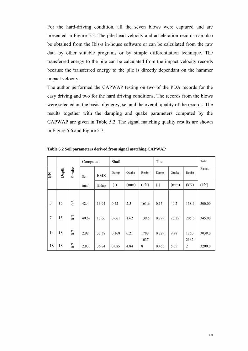
5-9
For the hard-driving condition, all the seven blows were captured and are
presented in Figure 5.5. The pile head velocity and acceleration records can also
be obtained from the Ibis-s in-house software or can be calculated from the raw
data by other suitable programs or by simple differentiation technique. The
transferred energy to the pile can be calculated from the impact velocity records
because the transferred energy to the pile is directly dependant on the hammer
impact velocity.
The author performed the CAPWAP testing on two of the PDA records for the
easy driving and two for the hard driving conditions. The records from the blows
were selected on the basis of energy, set and the overall quality of the records. The
results together with the damping and quake parameters computed by the
CAPWAP are given in Table 5.2. The signal matching quality results are shown
in Figure 5.6 and Figure 5.7.
Table 5.2 Soil parameters derived from signal matching CAPWAP
BN
Dep
th
Str
oke
Computed Shaft Toe Total
Set EMX Damp Quake Resist Damp Quake Resist
Resist.
(mm) (kNm) (-) (mm) (kN) (-) (mm) (kN) (kN)
3 15 0.3
42.4 16.94 0.42 2.5 161.6 0.15 40.2 138.4 300.00
7 15 0.3
40.69 18.66 0.661 1.62 139.5 0.279 26.25 205.5 345.00
14 18 0.7
2.92 38.38 0.168 6.21 1788 0.229 9.78 1250 3038.0
18 18 0.7
2.833 36.84 0.085 4.84
1037.
8 0.455 5.55
2162.
2 3200.0

5-10
Figure 5.5 IBIS-S Set Measurements for Hard-Driving Condition
40
50
60
70
80
90
100
47.5 52.5 57.5 62.5
Dis
plac
emen
t (m
m)
Time (s)
BN15BN16
BN14BN13
BN17BN18
BN19
Rebound
Penetration
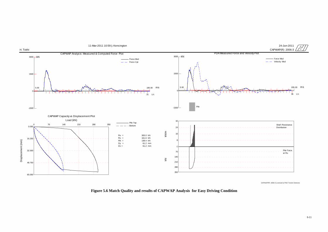
5-11
Figure 5.6 Match Quality and results of CAPWAP Analysis for Easy Driving Condition
5.00 180.00
-1500
0
1500
3000
CAPWAP Analysis: Measured & Computed Force Plot
ms
kN
31 L/c
Force Msd
Force Cpt
5.00 205.00
-1500
0
1500
3000
PDA Measured Force and Velocity Plot
ms
kN
36 L/c
Force Msd
Velocity Msd
Pile
0
8
16
24
32
kN/m
0
70
140
210
280
350
kN
Shaf t ResistanceDistribution
Pile Forceat Ru
0 70 140 210 280 3500.000
16.250
32.500
48.750
65.000
CAPWAP Capacity vs Displacement Plot
Load (kN)
Dis
pla
cem
en
t (m
m)
Pile Top
Bottom
Ru = 300.0 kNRs = 161.6 kNRb = 138.4 kNDy = 61.2 mmDx = 61.2 mm
Research Thesis; Pile: 89-EOD; Banut 6t; Blow: 183 (Test: 11-Mar-2011 10:59:); Kensington 24-Jun-2011
H. Tokhi CAPWAP(R) 2006-3
CAPWAP(R) 2006-3 Licensed to PDA Testing Services

5-12
Figure 5.7 Match Quality and results of CAPWAP Analysis for Hard Driving Condition
15.00 150.00
-2000
0
2000
4000
CAPWAP Analysis: Measured & Computed Force Plot
ms
kN
23 L/c
Force Msd
Force Cpt
15.00 225.00
-2000
0
2000
4000
PDA Measured Force and Velocity Plot
ms
kN
36 L/c
Force Msd
Velocity Msd
Pile
0
200
400
600
800
kN/m
0
700
1400
2100
2800
3500
kN
Shaf t ResistanceDistribution
Pile Forceat Ru
0 700 1400 2100 2800 35000.000
6.250
12.500
18.750
25.000
CAPWAP Capacity vs Displacement Plot
Load (kN)
Dis
pla
cem
en
t (m
m)
Pile Top
Bottom
Ru = 3198.3 kNRs = 1037.3 kNRb = 2161.0 kNDy = 17.6 mmDx = 20.0 mm
BENT ST KENSINGTON; Pile: 89-EOD; BANUT6-6T; Blow: 411 (Test: 11-Mar-2011 11:17:) 24-Jun-2011
H. Tokhi CAPWAP(R) 2006-3
CAPWAP(R) 2006-3 Licensed to PDA Testing Services

5-13
GRLWEAP analyses were also performed for the easy and hard driving
conditions and the Bearing Graph showing the ultimate capacity versus set is
presented in Figure 5.8.
0
500
1000
1500
2000
2500
3000
3500
10 20 30 40 50 60 70 80
Ult
imate
Cap
acit
y (k
N)
Set(mm)
Easy Driving, 300mm Stroke
Hard Driving,700mm Stroke
Figure 5.8 GRLWEAP Bearing Graph for Banut6T hammer
The GRLWEAP bearing graph shown in Figure 5.8 is only for single stroke.
However, a more general bearing graph can also be established for any particular
hammer. The Figure 5.9 and Figure 5.10 show the results of GRLWEAP analysis
at various strokes for the Banut 6t hammer.
The ratios of the Hiley, GRLWEAP and the CAPWAP capacities are also plotted
in Figure 5.9 and Figure 5.10. From Figure 5.9 it can be seen that the capacity
ratio of GRLWEAP and the CAPWAP for the easy-driving condition is about 0.9,
which indicates that, although the test results are consistent, GRLWEAP slightly
under predicts capacities in easy-driving conditions. However, in hard driving
conditions the ratios are nearly one, indicating the results are consistent and in
good agreement.

5-14
Figure 5.9 GRLWEAP Analysis for easy-driving condition. Hiley Correction Factor vs. Set
for Banut6T hammer, 350mm precast pile – Easy driving condition
Similarly, the ratio of Hiley to GRLWEAP (or CAPWAP) is approximately 1.35
which indicates that, irrespective of the driving conditions, the Hiley formula over
predicts the capacity by this factor and that this over estimation is consistent.
1.331.38
1.361.35
0.991.02
y = 2E-06x3 - 0.0002x2 + 0.0055x + 1.3R² = 0.9527
0.50
0.70
0.90
1.10
1.30
1.50
1.70
1.90
2.10
0.00 2.00 4.00 6.00 8.00 10.00 12.00 14.00 16.00 18.00 20.00
Co
rrec
tion
Fac
tor(
-)
Set(mm)
Hiley/GRLWEAP
Hiley/CAPWAP
GRLWEAP/CAPWAP
Figure 5.10 GRLWEAP Analysis for hard-driving condition. Hiley Correction Factor vs. Set
for Banut6T hammer, 350 precast pile – Hard driving condition
1.311.34
0.900.92
y = 2E-06x3 - 0.0002x2 + 0.0055x + 1.3R² = 0.9527
0.00
0.50
1.00
1.50
2.00
2.50
3.00
3.50
10.00 30.00 50.00 70.00 90.00 110.00 130.00
Co
rrec
tio
n F
acto
r(-)
Set(mm)
Hiley/GRLWEAP
Hiley/CAPWAP
GRLWEAP/CAPWAP
Poly. (Hiley/GRLWEAP)
Poly.
(Hiley/GRLWEAP)

5-15
The capacities calculated by the various methods such as the CAPWAP, Gates,
GRLWEAP, Hiley and MnDOT methods are plotted and shown in Figure 5.11.
The results show that the Hiley formula pile capacity predictions are very good
compared to the CAPWAP and consistent throughout the blow records. On the
other hand, Gates and MnDOT perform poorly for the easy driving condition, but
compare reasonably well in hard driving conditions. It should be mentioned that
the Hiley capacities in Figure 5.11are not factored.
0
500
1000
1500
2000
2500
3000
3500
4000
0 5 10 15 20 25 30 35 40 45 50
Cap
acit
y (k
N)
Set (mm)
Hiley (Ibis)
GRLWEAP
CAPWAP
Gates
MnDOT
Case Resistance (RMX)
Hard driving
Easy driving
Figure 5.11 Overall Comparisons of Capacities by CAPWAP, Hiley, Gates, GRLWEAP and
MnDOT Methods for the Easy and Hard Driving Conditions
The performance of the Banut hammer for the two driving conditions is shown in
Figure 5.12. It can be seen that the hammer is very efficient and that the efficiency
decreases slightly with increasing velocity.
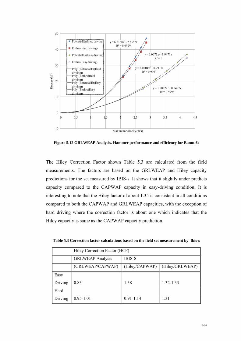
5-16
y = 6.6168x2 - 2.5387xR² = 0.9999
y = 6.0673x2 - 1.9471xR² = 1
y = 2.0004x2 + 0.2977xR² = 0.9997
y = 1.8072x2 + 0.5487xR² = 0.9996
-10
0
10
20
30
40
50
0 0.5 1 1.5 2 2.5 3 3.5 4 4.5
En
ergy
(kJ)
Maximum Velocity (m/s)
Potential Er(Hard driving)
Enthru(Hard driving)
Potential Er(Easy driving)
Enthru(Easy driving)
Poly. (Potential Er(Hard driving))Poly. (Enthru(Hard driving))Poly. (Potential Er(Easy driving))Poly. (Enthru(Easy driving))
Figure 5.12 GRLWEAP Analysis. Hammer performance and efficiency for Banut 6t
The Hiley Correction Factor shown Table 5.3 are calculated from the field
measurements. The factors are based on the GRLWEAP and Hiley capacity
predictions for the set measured by IBIS-s. It shows that it slightly under predicts
capacity compared to the CAPWAP capacity in easy-driving condition. It is
interesting to note that the Hiley factor of about 1.35 is consistent in all conditions
compared to both the CAPWAP and GRLWEAP capacities, with the exception of
hard driving where the correction factor is about one which indicates that the
Hiley capacity is same as the CAPWAP capacity prediction.
Table 5.3 Correction factor calculations based on the field set measurement by Ibis-s
Hiley Correction Factor (HCF)
GRLWEAP Analysis IBIS-S
(GRLWEAP/CAPWAP) (Hiley/CAPWAP) (Hiley/GRLWEAP)
Easy
Driving 0.83 1.38 1.32-1.33
Hard
Driving 0.95-1.01 0.91-1.14 1.31

5-17
5.8 Extended Application of IBIS-S
As mentioned earlier, the CAPWAP signal matching program does not produce a
unique solution due to the many unknown empirical parameters. Some of the
parameters are damping factors, quakes, toe gap and radiation damping.
Therefore, due to the high resolution and accuracy of the IBIS-S unit, it is possible
that some of these empirical parameters could be directly evaluated. Additionally,
it is possible to evaluate the integrity of driven piles from the velocity and
acceleration records, especially if a defect has been detected and the need to proof
test the untested piles.
Another very useful application of the IBIS-S radar, due to its multi-target
measurement capability, is in the assessment of pile mechanical joints. The
current VicRoads standard only requires visual inspection under many repetitive
hammer blows. In some situations PDA dynamic testing is done concurrently and
the results are checked with CAPWAP analysis to ensure the movement complies
with a given standard.

6-1
CHAPTER 6
6 CONCLUSION
6.1 Summary
The pile driving formulas were derived based on the Newtonian theory of impact.
In the past it has been known that the dynamic formula are not very accurate and
it consistently over estimate pile capacities. This is particularly true for the Hiley
formula.
The reason for this poor performance can be attributed to the fact that often the
hammer energy delivered to a pile is estimated rather than determined on case by
case bases. It has been shown that this energy can vary enormously from pile to
pile and assuming energy to be constant for a given hammer is incorrect. The
second reason for the poor results of the dynamic formula is the set and temporary
compressions are not determined accurately in the field, and hence lead to
erroneous capacity results. The third reason, and the most important, is that the
dynamic formula does not account for the dynamic effects, which is similar to the
damping factors in the wave equation treatments. Not to mention the fact that in
almost all researches, the capacity comparison between dynamic formula and the
static testing is deemed to be incorrect because of the time difference of testing
and the phenomenon of setup – capacity gain over time.
In this research all these factors have been addressed and tests were undertaken
that showed the dynamic formula can be used with greater confidence and can
provide comparable results to the wave equation method. Chapter 2 presents the
application of dynamic pile testing methods. Chapter 3 compiles a collection of

6-2
results on the performance of pile driving formula reported in the literature.
Chapter 4 includes a comprehensive numerical analysis of 1944 systematic cases
by wave-equation based software called GRLWEAP and factors were calculated
for each case to be used in the dynamic formula to account for the dynamic
effects. Chapter 5 presents the results of field study as well as measurement
results using radar equipment proposed in this research. Further analysis results
using CAPWAP and GRLWEAP programs were carried out and a comparison of
the results are presented.
The field test data gathered during field test of IBIS-S radar provide an excellent
basis for the evaluation of the Hiley formula in prediction of pile capacity for all
driving conditions. A comparison of the predictions obtained from the pile driving
formulae with the higher order methods such the CAPWAP and GRLWEAP
wave-equation analysis showed that the results are very consistent and accurate.
The present investigation thus demonstrates that the pile capacity prediction by
the Hiley formula are very reliable provided the variation in the energy input can
be accurately measured and allowed for in the calculations. Since under normal
pile driving conditions, variability in the driving system and the energies delivered
to the pile exists, it is important to account for this variability so that the driving
formula can be used with greater confidence.
The results of the correlations between the wave equation and the dynamic
formulas are both surprising and very informative. As noted in chapter 4, Table
4.13 and Table 4.14, the ratio of the resistance predicted by the Hiley formula and
the wave equation is rather constant. This would indicate that at least for these
cases the Hiley formula the consistency is quite surprising, especially considering
the amount of research which has been published condemning the method. This is
not to imply that the dynamic formulas are without proponent.
In the past the poor quality of the results obtained by pile driving formula was
partly related to the erroneous estimate of the driving energy. It is now possible,
with the aid of new technology, to measure with high accuracy not only the
energy delivered to the pile by each blow, but also the full pile displacement
records.

6-3
A correction factor to allow for the dynamic effects, similar to the Case damping
factor, was back-calculated from the CAPWAP and GRLWEAP analysis. It
showed that the correction factor is quite consistent and can be developed for a
variety of ground conditions, hammers and pile types. This will allow for the
dynamic formula, particularly the Hiley formula to be used with greater accuracy
comparable to the wave equation analysis.
More general conclusion of the study in this paper can be as follows:
• The wave-equation analysis only describes the energy transfer mechanism
from the hammer to the pile toe in a systematic and accurate fashion and if
the dynamic formulae are modified to account for the energy losses, then
the dynamic formulae should technically fulfil the same function.
• The dynamic formulae, which ignore the dynamic effects, need to be
accounted for in the formulae.
• The energy delivered to the pile and its set measurements need to be
accurately determined in order to render the dynamic formulae reliable.
• Create a comprehensive database with driving records for various soil
conditions, driving systems as well as different piles and establish driving
formula correction factors against the database.
• The correction factors can be established from GRLWEAP and CAPWAP
analysis as well as static testing results.
6.2 Future Research
US department of transport (FHWA, FDOT, MnDOT, OSDOT, TRB and
WSDOT) are still heavily involved in research into pile driving formula. MnDOT
recently published a modified version of the Gates formula, while other works are
still ongoing. The current emphasis is to create comprehensive pile databases
based on the pile load tests and dynamic testing and to calibrate various pile
driving formulae against the database in order to establish the most suitable
formula.

6-4
Further investigation is required to determine the extent and the influence of
different damping factors and cushion materials. The investigation of this zone
can provide insight into the energy transfer into the pile.
Further study is required to better understand the distribution of the resistance
around and at the base of the pile. Also the effects of pore water pressure and time
on the resistance of pile will also need to be investigated.

A-1
Appendix A
Stress Wave Theory in Solid Media
Derivation of Wave Equation
A slender pile with uniform cross-section will transmit a pulse or wave down the
pile when mechanically impacted by a hammer on the top. It is assumed that
because of the much lower stiffness of the surrounding soil, the wave pulse can
only travel along the pile axis. Given the distance z measured from the pile head
down, let’s consider an infinitesimal pile element with length dz bounded by two
sections
The element is subjected to an external (soil) shear stress qs applied along the pile
shaft. Hence applying Newton’s second law to this infinitesimal element yields
𝐹 − (𝐹 + 𝑑𝐹) − 𝑞 𝑎 𝑑𝑧 = 𝜌𝐴𝑑𝑧 𝜕 𝑤𝜕𝑡 A.1
Where 𝑎 is the surface area, ρ is mass density of pile and w (z, t) is the axial
displacement of cross section at distance z and time t.
Rearrangement and substitution of the elastic stress-strain equation σ=Eε results
in the governing differential equation for the pile problem
𝐸 𝐴 𝜕 𝑤𝜕𝑧 − 𝑞 𝑎 = 𝜌𝐴 𝜕 𝑤𝜕𝑡 A.2
Assuming that there is no external force acting on the pile (qs=0), the above
equation can be rewritten in the familiar one-dimensional wave equation
∂2w∂t2 -c2 ∂2w∂z2 =0, where c= Ep ρ⁄ A.3
qs
z dz
Force F(z)=F Force F(z+dz)=F+dF

A-2
Solution and Interpretation of Wave Equation
The following is an excerpt from Timoshenko (1951) and Verruijt (2005), which
explain the interpretation of the stress-wave propagation equation applicable to
dynamically loaded piles.
Sudden loading or displacement caused by a force on an elastic solid media
generates stress waves that radiates from the impact point in all directions with
finite velocities of propagation. Usually there is more than one type of wave with
more than one wave velocity. The simplest representation of wave motion in
special cases, such as in piles, can be approximated with the one-dimensional
hyperbolic partial differential equation in the form shown above.
The one-dimensional wave equation is easily solvable by the various
mathematical methods such as Laplace, Separation of Variables and Method of
Characteristics. It can be shown by simple substitution that any function in the
form of f(z-ct) is a solution of the partial differential equation. By the same token,
g(z+ct) is also a solution and because the partial different general solution can be
given by
𝑤(𝑧, 𝑡) = 𝑓(𝑧 − 𝑐𝑡) + 𝑔(𝑧 + 𝑐𝑡) A.4
The first and second terms of the general solution in equation A.4 represent stress
wave travelling in the downward and upward directions, respectively, with
constant speed c.
When soil friction resistances are introduced into the partial differential equation,
then the solution is neither simple nor practical, except for very simple cases.
In the case where there is ground shear resistance, the solution for above
differential equation is carried out by numerical finite difference method and in
fact the Smith’s approximation in itself turns out to be essentially a finite
difference technique.
An interesting aspect of the wave propagation in solid media is reflection and
transmission of waves at the surface of discontinuity or change in material

A-3
property. Hence, essentially two boundary conditions of interest in pile dynamic
are waves approaching free and fixed ends.
When a pulse approaches a free end, there is not inertial mass to overcome, and
the energy cannot continue to travel, instead it reflects back. At the exact moment
of reflection, the velocity doubles and a compressive wave is reflected as a similar
tension wave, and vice versa.
On the other hand, when a pulse approaches a fixed end, the section remains
immovable and the wave is reflected without any change.
CAPWAP Notation
The notation of CAPWAP parameters is defined in the CAPWAP manual 2006
(PDI, 2006) and the relevant section has been reproduced.
BT Toe radiation damping. This is the energy radiated by surrounding soil as a
result of pile motion A radiation damping model by introducing additional
soil mass (MS) and dashpots to represent soil motion to obtain better
correlation with static load testing.
CS Shaft quake multiplier. This is used to make unloading lower than the
loading quake. The default value of 1 makes loading and unloading
equal. It normally varies between 0.1 and 1.0.
CT Toe quake multiplier. Same as CS.
JS Shaft damping factor (case). It is a non-dimensional factor that is
independent of the static resistance.
JT Toe damping factor (case)
LS Shaft reloading.
LT Toe reloading
MS Shaft radiation mass. This value of this is dependent on the size of pile.
The recommended default value corresponds to a cylinder of soil
surrounding the pile and being roughly 0.3m thick.
MT Toe radiation mass. Also see MS.

A-4
OP Toe damping type option (0=linear viscous, 1=Smith, 2=combination).
The Smith calculation yields better signal match. OP=2 is most frequently
used to improve the match around the 2L/c i.e. return wave after impact.
PL Toe plug. This is the mass of soil sticking or trapped underneath the pile
causing inertial force thus making the pile appear longer.
PS Shaft plug
QS Shaft quake. Quake or displacement is none zero value with maximum
being 10mm and most commonly around 2.5 to 5.0mm.
QT Toe quake. Maximum value of 25mm or more.
SO Shaft damping type option (0=linear viscous, 1=Smith, 2=combination).
Also see OP.
SL Shaft radiation damping. Also see BT.
SS Smith shaft damping. The traditional Smith damping that is a velocity and
static resistance. However, it is more convenient to use linear viscous
coefficients rather than the Smith values so that they can be assigned
independent from the magnitude of the static resistance.
ST Smith toe damping.
TG Toe gap. A gap beneath a pile toe driven in very hard end bearing. It exists
prior to rebound as it starts to move down again without any resistance.
UN Shaft unloading multiplier. It varies between 0 and 1; with UN=0 there is
no downward directed shaft resistance during pile rebound; hence it is
applicable in easy driving condition.

A-5
CAPWAP Parameters and Definition
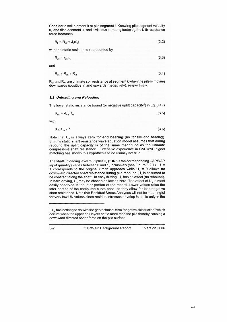
A-6

A-7

A-8

A-9

B-1
Appendix B
Derivation of Dynamic Formula
The following section from Chellis (1951) is reproduced.
The momentum of the ram at the moment of impact is Wrv/g, where v is ram
velocity at moment of impact. At the end of the period of compression the
momentum of the ram is (Wrv/g) – Mt, and the velocity vc = [(Wrv/g) – Mt]/
(Wr/g). Assuming that the pile is able to move a short distance, and that the
hammer blows and rebounds of the pile result in a looseness between the pile and
the earth, then the momentum of the pile at the end of the period of compression
may be taken as Mt, and the velocity of the pile becomes vc=Mt/(Wp/g).
Since the velocities of the ram and pile are equal at the end of the compression
period, at that time Mt=vW r Wp/g(Wr+Wp).
At the end of the period of restitution, the momentum of the ram is (Wrv/g)-Mt-
eMt=Wrvr/g; therefore,
𝑣 = 𝑣 − 𝑀 (1 + 𝑒)𝑊 𝑔⁄ = 𝑣 − 𝑊𝑊 + 𝑊 𝑣(1 + 𝑒)= 𝑊 − 𝑒𝑊𝑊 + 𝑊 𝑣
B.1
At the end of the period of restitution, the momentum of the pile is Mt + eMt =
Wpvp/ g; therefore,
𝑣 = 𝑀 (1 + 𝑒)𝑊 𝑔⁄ = 𝑊𝑊 + 𝑊 (1 + 𝑒)𝑣 = 𝑊 + 𝑒𝑊𝑊 + 𝑊 𝑣 B.2
Using the above values for vr and vp, it is possible to determine the sum of the
gross energies in the ram and pile, at the end of the period of restitution, available
for expenditure in overcoming ground resistance to driving, and in causing
temporary elastic compressions in the driving cap, pile, and soil.
The energy available in the ram and pile at the close of the period of restitution
will be equal to

B-2
𝑊2𝑔 𝑣 + 𝑊2𝑔 𝑣 = 𝑊 𝑣2𝑔 𝑊 − 𝑒𝑊𝑊 + 𝑊 + 𝑊 𝑣2𝑔 𝑊 + 𝑒𝑊𝑊 + 𝑊
= 𝑊 𝑣2𝑔 (𝑊 + 𝑒 𝑊 )(𝑊 + 𝑊 )
= 𝑊 ℎ 𝑊 𝑒 𝑊𝑊 + 𝑊 B.3
If the above equation for energy available at the close of the period of restitution
is written as
𝑊 𝑣2𝑔 1 − 𝑊 (1 − 𝑒 )𝑊 + 𝑊 B.4
Then the loss in energy due to impact is
𝑊 𝑣2𝑔 𝑊 (1 − 𝑒 )𝑊 + 𝑊 = 𝑊 ℎ 𝑊 (1 − 𝑒 )𝑊 + 𝑊 B.5
And the efficiency of the hammer blow is
𝑊 + 𝑒 𝑊𝑊 + 𝑊 = 11 + 𝑊 𝑊⁄ + 𝑒1 + 𝑊 𝑊⁄ B.6
(Because of smallness of the term e2compared to 1, the efficiency has been taken
as to serve as the basis of the expression in the denominators of the Eytelwein and
Navy-McKay formulas, in each of which, however, it has been modified
empirically.)
If not impact or elastic losses occurred, and the mechanical efficiency of the
hammer were 100 per cent (e.g. no losses), then following expression could be
written
𝑅 𝑠 = 𝑊 ℎ B.7
Denoting the mechanical efficiency by the term ef , the above expression becomes
𝑅 𝑠 = 𝑒 𝑊 ℎ B.8

B-3
Replacing the terms ��� by the expression derived for energy available at the
close of the period of restitution,
𝑅 𝑠 = 𝑒 𝑊 ℎ 𝑊 + 𝑒 𝑊𝑊 + 𝑊 B.9
This may be transposed to read
𝑅 = 𝑒 𝑊 ℎ𝑠 𝑊 + 𝑒 𝑊𝑊 + 𝑊 B.10
However, while the tip of the pile moves downward a distance s, the top of the
driving cap moves downward an additional distance C1+C2+C3 owing to
temporary elastic compression in the cap, pile, and soil. Within elastic limits, the
deformation of each of those materials may be assumed to vary with load. For the
cap and pile, the amounts of temporary compression may be computed from
expression 𝐶 = 𝑅 𝑙 𝐴𝐸⁄ . The work obtained from the kinetic energy of the blow
may be written, instead of Rus as Ru(s+C/2), and the above expression becomes
𝑅 = 𝑒 𝑊 ℎ𝑠 + 𝐶 2⁄ 𝑊 + 𝑒 𝑊𝑊 + 𝑊 B.11
If the temporary compression C is subdivided into its component elements the
following expression results:
𝑅 = 𝑒 𝑊 ℎ𝑠 + (𝐶 + 𝐶 + 𝐶 ) 𝑊 + 𝑒 𝑊𝑊 + 𝑊 B.12
Since there are losses due to efficiency, impact, and elastic compressions of the
cap, pile, and soil, these items are deducted as shown in the following expression:
𝑅 = 𝑒 𝑊 ℎ𝑠 − 𝑒 𝑊 ℎ 𝑊 (1 − 𝑒 )𝑊 + 𝑊𝑠 − 𝑅 𝐶2𝑠 − 𝑅 𝑙2𝐴𝐸𝑠− 𝑅 𝐶2𝑠
B.13
And, callingRul AE=C2⁄ , by combining terms, we obtain

B-4
𝑅 = 𝑒 𝑊 ℎ𝑠 + (𝐶 + 𝐶 + 𝐶 ) 𝑊 + 𝑒 𝑊𝑊 + 𝑊 𝐻𝑖𝑙𝑒𝑦 𝑓𝑜𝑟𝑚𝑢𝑙𝑎 B.14
If the rebound coefficients in formula (hiley formula) are modified empirically,
and a factor of safety of 3 is assumed, the following Canadian National Building
Code formula is obtained:
𝑅 = 4𝑛𝑊 𝐻𝑠 + 𝐶 2⁄ 𝐶𝑎𝑛𝑎𝑑𝑖𝑎𝑛 𝑁𝑎𝑡𝑖𝑜𝑛𝑎𝑙 𝐵𝑢𝑖𝑙𝑑𝑖𝑛𝑔 𝐶𝑜𝑑𝑒 𝑓𝑜𝑟𝑚𝑢𝑙𝑎 B.15
Where 𝑛 = for friction piles = . for refusal
𝐶 = 3𝑅𝐴 𝑙𝐸 + 0.0001) H=hammer drop height in feet If it is assumed that there are no elastic losses in the cap or soil quake, formula
(hiley) reduces to
𝑅 = 𝑒 𝑊 ℎ𝑠 − 𝑒 𝑊 ℎ 𝑊 (1 − 𝑒 )𝑊 + 𝑊𝑠 − 𝑅 𝑙2𝐴𝐸𝑠 B.16
Now assume the hammer to be mechanically 100 per cent efficient, thus omitting
the term 𝑒 , and solve for 𝑅 , in which case,
𝑅= 𝐴𝐸𝑙 −𝑠+ 𝑠 + 𝑊 ℎ 𝑊 + 𝑒 𝑊𝑊 + 𝑊 2𝑙𝐴𝐸 𝑈𝑛𝑖𝑣𝑒𝑟𝑠𝑎𝑙 𝑜𝑟 𝑆𝑡𝑒𝑟𝑛 𝑓𝑜𝑟𝑚𝑢𝑙𝑎
B.17
If the impact is assumed to be perfectly inelastic instead of semi elastic, then 𝑒 = 0, and above formula becomes

B-5
𝑅= 𝐴𝐸𝑙 −𝑠+ 𝑠 + 𝑊 ℎ𝑊 + 𝑊 2𝑙𝐴𝐸 𝑅𝑒𝑑𝑡𝑒𝑛𝑏𝑎𝑐ℎ𝑒𝑟 𝑓𝑜𝑟𝑚𝑢𝑙𝑎
B.18
If the temporary elastic shortening of the ground is included, as well as of the pile,
and these are measured from a load-test diagram near to or beyond the failure
point, the above formula becomes
𝑅= 𝑠𝑡𝑎𝑛 ∅ −1+ 1 + 𝑊 ℎ𝑊 𝑊 2 𝑡𝑎𝑛 ∅𝐴𝐸 𝑆𝑐ℎ𝑒𝑛𝑘 𝑓𝑜𝑟𝑚𝑢𝑙𝑎
B.19
Where ��= tangent of the gradient of load settlement curve.
If the impact loss is entirely neglected, the Redtenbacher formula becomes
𝑅 = 𝑊 ℎ𝑠 𝑊𝑊 + 𝑊 𝑅𝑖𝑡𝑡𝑒𝑟 𝑓𝑜𝑟𝑚𝑢𝑙𝑎 B.20
𝑅= − 𝑠𝐴𝐸𝑙 + 2𝑊 ℎ𝐴𝐸𝑙 + 𝑠𝐴𝐸𝑙 𝑊𝑒𝑖𝑠𝑏𝑎𝑐𝑘 𝑓𝑜𝑟𝑚𝑢𝑙𝑎
B.21
If the hammer is assumed to be mechanically 100 percent efficient, thus emitting
the term ef, and if, instead of considering the elastic losses in the cap or soil
quake, twice the elastic loss is used, taking into account the full length of the pile,
and if fixed values are assumed for e, then the Hiley formula becomes

B-6
𝑅= 12𝑊 ℎ 𝑊 + 𝐾𝑊𝑊 + 𝑊𝑠 + 24000𝑅 𝑙𝐴𝐸 𝐼𝑛𝑡𝑒𝑟𝑛𝑎𝑡𝑖𝑜𝑛𝑎𝑙 𝐶𝑜𝑛𝑓𝑒𝑟𝑒𝑛𝑐𝑒 𝑈𝑛𝑖𝑓𝑜𝑟𝑚
Building Code formula
B.22
Where K= 0.25 for steel and 0.1 for other piles.
On the other hand, assume the impact to be perfectly elastic, and also assume that
the pile is fully embedded in the ground and is a friction pile without end bearing,
so that the distance from the toe to the centre of resistance is 𝑙/2, and the Stern
formula become
𝑅 = 2𝐴𝐸𝑠𝑙 1 + 𝑊 ℎ𝑙𝑠 𝐸𝐴 − 1 𝑅𝑎𝑛𝑘𝑖𝑛𝑒 𝑓𝑜𝑟𝑚𝑢𝑙𝑎 B.23
By taking the Hiley formula and assuming that the mechanical efficiency is 100
percent (ef=0), that the impact is perfectly inelastic (e=0), and that there are no
elastic losses in the cap, pile, or soil, we obtain
𝑅 = 𝑊 ℎ𝑠 𝑊𝑊 + 𝑊 𝐷𝑢𝑡𝑐ℎ 𝑓𝑜𝑟𝑚𝑢𝑙𝑎 B.24
The Ritter formula is the same as the Dutch formula, with the inclusion of terms
to add the weight of the pile and ram:
By writing the Dutch formula in the following form, taking h in feet, and
assuming a factor of safety of 6, we obtain a formula for drop hammers:
𝑅 = 2𝑊 𝐻𝑠 1 + 𝑊𝑊 𝐸𝑦𝑡𝑒𝑙𝑤𝑒𝑖𝑛 𝑓𝑜𝑟𝑚𝑢𝑙𝑎 B.25
The Eytelwein formula is modified as follows for single-acting and double acting
hammers:
Single-acting: 𝑅 = .

B-7
Double-acting: 𝑅 = ( ).
Where A= effective area of piston,
p= air of steam pressure.
If H is taken in feet, a factor of safety of 6 assumed, and the ratio Wp Wr⁄ in the
above formula modified by 0.3s instead of 0.1, we have
𝑅 = 2𝑊 𝐻𝑠 1 + 0.3 𝑊𝑊 𝑁𝑎𝑣𝑦 − 𝑀𝑐𝐾𝑎𝑦 𝑓𝑜𝑟𝑚𝑢𝑙𝑎 B.26
If in Hiley formula the impact loss is entirely neglected, the mechanical efficiency
taken as 100 percent, the elastic losses in the cap, pile and soil represented by a
constant term of 1.0, H taken in feet and then multiplied by 12, and a factor of
safety of 6 is assumed, the following expression is obtained for use with drop
hammers:
𝑅 = . 𝐸𝑛𝑔𝑖𝑛𝑒𝑒𝑟𝑖𝑛𝑔 𝑁𝑒𝑤𝑠 𝑓𝑜𝑟𝑚𝑢𝑙𝑎 B.27
For use with single-acting hammers, the above formula was modified by its author
by changing the term 1.0 to 0.1, and in this form as given below has been widely
used for single-acting, double-acting and differential-acting hammers:
Single-acting: 𝑅 = 2𝑊 𝐻𝑠 + 1.0
Double and differential acting: 𝑅 = 2𝐸𝑠 + 0.1
The above formulas may be expressed as follows, n being the number of blows
per foot penetration:
Single-acting:

B-8
𝑅= 20𝑛120 + 𝑛 𝑊 𝐻 𝑉𝑢𝑙𝑐𝑎𝑛 𝐼𝑟𝑜𝑛 𝑊𝑜𝑟𝑘𝑠 𝑓𝑜𝑟𝑚𝑢𝑙𝑎 B.28
Double and differential acting: R= 20n120+n En
The United States Steel Co. modifies the Engineering News formula by varying
the constant in the numerator, as follows:
Drop hammers:
𝑅= 𝐹𝐻𝑊𝑠 + 1.0 𝑈𝑛𝑖𝑡𝑒𝑑 𝑆𝑡𝑎𝑡𝑒𝑠 𝑆𝑡𝑒𝑒𝑙 𝑓𝑜𝑟𝑚𝑢𝑙𝑎
B.29
Single-acting: 𝑅 = 𝐹𝐻𝑊𝑠 + 0.1
Double and Differential-acting: 𝑅 = 𝐹𝐻(𝑊 + 𝐴𝑝)𝑠 + 0.1
Where F=2 for piles driven to refusal or practical refusal;
=6 for piles driven easy in sands and gravels;
=4 for piles driven easily in hard or sandy clays;
=3 for piles driven easily in mixed medium clays and sand or sand and
silt;
=2 for piles driven easily in alluvial deposits;
A= effective piston area;
p= mean steam or air pressure;
Another modification of formula is

B-9
𝑅= 2𝑊 𝐻𝑠 + 0.3 𝐵𝑢𝑟𝑒𝑎𝑢 𝑜𝑓 𝑌𝑎𝑟𝑑𝑠 𝑎𝑛𝑑 𝐷𝑜𝑐𝑘𝑠 𝑓𝑜𝑟𝑚𝑢𝑙𝑎 B.30
The Benabencq formula is
𝑅 = 𝑊 𝐻2𝑠 + 𝑊 + 𝑊 𝐺𝑜𝑜𝑑𝑟𝑖𝑐ℎ 𝑓𝑜𝑟𝑚𝑢𝑙𝑎 B.31
The Sanders formula, proposed in 1851, was obtained by applying a purported
factor of safety of 8 to formula ( ),
𝑹 = 𝑾𝒓𝒉𝟖𝒔 𝑺𝒂𝒏𝒅𝒆𝒓𝒔 𝒇𝒐𝒓𝒎𝒖𝒍𝒂 B.32
And Merriman used the same terms with a purported factor of safety of 6,
𝑹 = 𝑾𝒓𝒉𝟔𝒔 𝑴𝒆𝒓𝒓𝒊𝒎𝒂𝒏 𝒇𝒐𝒓𝒎𝒖𝒍𝒂 B.33
The Goodrich formula is a simplification of a comprehensive formula which
contains 25 terms covering conditions of the pile, hammer, cap and ground, and
was intended for use only with wood piles and drop hammers with a fall of about
15 ft and set of 1.0 in. Under these conditions it was believed by its author to have
accuracy within 10 per cent of that of the comprehensive formula.
𝑅 = 10𝑊 𝐻3𝑠 𝐺𝑜𝑜𝑑𝑟𝑖𝑐ℎ 𝑓𝑜𝑟𝑚𝑢𝑙𝑎 B.34
The Kafka formula is the earliest form in which the elastic rebounds of the pile
and soil, measured from a graph taken on the pile, have been found. This formula
is
𝑅 = 𝑋 −1 + 1 + 𝑌𝑋(2𝑠 + 𝜆) + 𝑊
+ 𝑊 𝐾𝑎𝑓𝑘𝑎 𝑓𝑜𝑟𝑚𝑢𝑙𝑎
B.35
where 𝑋 = (2𝑠 + 𝜆)
𝑌 = 6𝑊 ℎ
𝜆 = 𝑠 + 𝐶 + 𝐶

C-1
Appendix C
GRLWEAP Background features and Parameters
GRLWEAP Input
The following sections have been re-produced from the GRLWEAP Help Menu.
GRLWEAP was programmed for simple input preparation. Known parameters
such as pile length, skin friction distribution, etc. can be entered directly and the
program will calculate the necessary model parameters. Since hammer modelling
requires the input of relatively complex information, data has been prepared and
stored on a file for the most commonly encountered hammer models. Thus, after a
hammer has been selected the GRLWEAP hammer model is complete.
� 1.1 Input of Static Soil Resistance
� 1.2 Quake Input
� 1.3 Soil Damping Input
� 1.4 Hammer Data Input
� 1.5 Hammer Parameters
� 1.6 Driving System Data
1.1 Input of Static Soil Resistance
The basic wave equation process requires input of static and dynamic soil
resistance parameters. Depending on the Analysis Type, standard static soil
parameters may include unit shaft resistance and end bearing or total capacity and
static toe/shaft resistance percentage, shaft resistance distribution, and quakes.
The dynamic shaft resistance is specified through damping options and damping
factors. For the input of the static soil resistance, GRLWEAP offers the following
options:
a) For a Bearing Graph
- Up to 10 ultimate capacities
- Shaft resistance percentage whereby, for the second and later ultimate capacity
values
analysed, the option exists of:
- varying the shaft and toe resistance proportionally
C-2
- varying only the shaft resistance
- varying only the toe resistance
- Shaft resistance distribution
- either simple rectangular or triangular or as a variable distribution
- the distribution is shifted along the pile using the penetration input
1.2 Quake Input
Usually a 0.1 inch (2.5 mm) value is a reasonable input for the shaft quake; this
value has been used extensively with good correlations. Measurements have
demonstrated that the toe quake can be much larger than 0.1 inches or 2.5 mm.
Particularly for displacement piles with a width or diameter of more than 12
inches (300 mm), it is reasonable to assume a toe quake of at least D/120 or even
D/60, where D is the width of diameter of the pile. The larger value is reasonable
for soft or submerged soils. For open ended pipes, the situation is even more
complicated since the pile may or may not plug during driving; for coring or
unplugged driving, the usual 0.1 inch (2.5 mm) quake is appropriate. In a restrike
test and under static loading conditions, the soil may plug inside the pile bottom.
Then D/120 is again a reasonable quake assumption. Large quakes can
substantially influence the wave equation results, particularly tension stresses for
low resistance values and blow counts for high capacities. Unfortunately, large
quakes cannot be predicted from a mere inspection of subsurface investigation
data. Instead, large quakes are computed by analysis of dynamic measurements
taken during driving or re-striking. When piles are being driven into hard rock, it
may be necessary to reduce the quake to values less than 0.1 inches (2.5 mm) to
avoid under-predicting the capacity and stresses. Also, for piles with small toe
diameters of less than 12 inches (300 mm), or for tapered piles, input of a reduced
toe quake may be advisable. It is, however, suggested that quakes never be chosen
less than 0.04 inches (1 mm). For vibratory pile driving, a doubling of standard
quake values is recommended for cohesive soil. See Help/Soil Information/Soil
Parameters and Damping/Quakes for more specific information.
1.3 Soil Damping Input
Input of one average value for shaft damping and one value for toe damping using
the standard Smith Damping approach normally yields sufficient accuracy for
Bearing Graph or Inspector's Chart analyses. Damping forces are then calculated
by GRLWEAP as: with j, i.e. the so-called Smith damping factors, the same value

C-3
for all skin elements, Rs effectively normalizes the damping distribution. When
assigning an average shaft damping value, it should be remembered that damping
forces will be higher where there is a higher static resistance (it has at first a zero
value and varies with the pile displacement). The ST static soil resistance analysis
calculates reasonable averages.
1.4 Hammer Data Input
Hammer parameters are stored in the hammer data file for most commonly
encountered hammer models. All the user has to do is select the desired model. If
the hammer model is not contained in the file, the hammer must be coded using
the file maintenance program. The data in the hammer file reflects the best
knowledge on hammer performance available to the program authors. Actual field
performance of a hammer will depend on a variety of operational factors such as
its state of maintenance, or the fuel or power supply. Hammer design parameters
are also frequently modified. It is therefore imperative that the user insures
agreement between predicted and actual hammer performance by field inspection.
If necessary, file data may be modified by the user to adjust certain values.
However, it is preferable that the user leaves the file data unchanged and uses the
Hammer Parameters input under Options to modify parameters such as efficiency,
maximum pressure, or stroke.
1.5 Hammer Parameters
� 1.5.1 Hammer Efficiency
� 1.5.2 Diesel Hammers (OED and CED)
� 1.5.3 External Combustion Hammers (ECH)
1.5.1 Hammer Efficiency
The efficiency value accounts for unknowns in the model of hammer and impact
process and reduces the potential (usually the rated) energy to the kinetic energy
just before impact. The efficiency values can be highly controversial giving the
impression that one hammer make is more efficient than another. This is not
necessarily so. For example, a hammer with internal ram velocity monitoring may
have an assigned efficiency of 0.95, which GRLWEAP applies to the ram energy
just before impact, when all other hammer losses have been taken into account by
the ram velocity measurement. The hammer may have lost a considerable amount
of energy during the ram's downward movement; however, using the measured

C-4
ram velocity as a rating, only small additional losses have to be covered by the
efficiency input which is therefore relatively high.
1.5.2 Diesel Hammers (OED and CED)
In the data file, all diesel hammers have been assigned a hammer efficiency of 0.8.
Differences between individual types are compensated for in the analysis process.
Since diesel hammers are continuously analyzed starting at the time when the
compression cycle starts which happens a significant time interval prior to impact,
the reduction of the ram velocity corresponding to the efficiency happens just
before impact. Stroke for open end diesel hammers, and bounce chamber pressure
for closed ended diesel hammers, gives a good indication of actual hammer
performance. Also, blow rate as printed by the program may be used for
construction control, and an automatic stroke indicator (Saximeter™) is a good
tool for the purpose of measuring blow rate in the field. However, a hammer in a
very poor state of maintenance may have friction losses of such magnitude that
blow rate is not an accurate indicator of stroke. It has been noticed that
GRLWEAP tends to under-predict strokes, on occasion up to 20%, while stresses
and transferred energies are realistic. It is therefore suggested not to adjust the
stroke, e.g. by analyzing with an increased combustion pressure, unless the stroke
under-prediction exceeds 20%. This is reasonable and conservative particularly
when high strokes are possibly the result of pre-ignition. A diesel hammer will
perform particularly poorly when it overheats during hard driving and then pre-
ignites. Pre-ignition produces large strokes and low transferred energies, and
therefore high blow counts. This condition can be modeled by the program using a
negative combustion delay for liquid fuel injection or a reduced combustion start
volume for atomized injection (Options/Hammer Parameters). Pre-ignition is
usually an unexpected situation and cannot be detected in the field without
electronic measurements. A number of models; for example, the DELMAG, FEC,
and APE D-series hammers and the ICE I-series hammers; have stepwise
adjustable fuel pumps. For those hammers, a reduced fuel setting may be chosen
under Options/General Options/Stroke (only accessible if a diesel hammer was
selected). The Combustion Pressure input can also be adjusted by either changing
the absolute pressure value or the percentage in the main input screen or changing
both vs. the Depth values for the Driveability analysis. Input of fuel settings less
than maximum cause the program to choose a reduced maximum combustion
pressure. This input is really only meaningful for hammers that have a stepwise

C-5
adjustable fuel pump. Measurement results are limited; therefore, predictions
involving diesel hammers should be backed up by field control, particularly where
pile stress limitations are critical. It is the user's responsibility to check the actual
fuel settings used in the field. For hammers which do not have stepwise adjustable
fuel pumps and where reduced hammer energy is necessary or desirable, it is
recommended that constant stroke analyses be run, with iteration on pressure, for
a variety of strokes. In the field, the desirable stroke or bounce chamber pressure
is then attained by fuel pump adjustment.
1.5.3 External Combustion Hammers (ECH)
The wave equation model of ECH hammers is not as complicated as that for
diesel hammers, but the correct choice of a proper efficiency, i.e. impact velocity,
is not a simple task. For example, a thick cushion may produce a reduced stroke
while a thin cushion may allow for early air, steam, or hydraulic injection, i.e.
preadmission, and therefore self-cushioning.The ECH category includes an ever
increasing number of hammer systems, makes, and models, starting from the
simple cat-and-rope driven drop hammer of an SPT rig to sophisticated,
hydraulically powered hammers with pneumatic accelerators and electronic
controls. Naturally, the unknowns vary widely for these hammers and efficiency
values cannot possibly be assigned based on hammer model evaluations or a few
measurements at the time of a hammer model's introduction into construction
practice. Additional verification and, if needed, modification of the database-
supplied values are therefore strongly recommended. Efficiencies were assigned
as follows: Options/Numeric for hammer and pile cushions; under Options/Pile
Parameters/Additional Input for the pile top; and under Options/Pile
Parameters/Splices for cracks, slacks or splices. The input of the Elastic Modulus
of a cushioning material may be taken as one half of the tangent modulus
determined at a stress level of 5 ksi (35 MPa). The Tables of Helmet and Hammer
Cushion Properties and the Table of Cushion Material Properties contain moduli,
taken from a variety of sources and reduced by multiplication with 0.5. These
sources usually do not reveal how the tests were done or how the moduli were
calculated; however, results using the GRLWEAP recommended values are
generally acceptable.
(a) 0.67 for traditional single acting air/steam/hydraulic hammers where the
motive fluid enters the
C-6
power cylinder through valves controlled by the falling ram.
(b) 0.50 for the same hammer as in (a) but double, differential, or compound
acting.
(c) 0.95 for all hammers with electronic readout of energy shortly before impact
and where this energy
is the basis of the wave equation, or equivalent, stroke input.
(d) 0.80 for all other hydraulic hammers where measurements have shown that
preadmission is
precluded and that the downward acceleration will not cause uplift in hard
driving.
Note: The user is urged to verify that these efficiency values yield reasonable
results. GRL efficiency assignments shall not be used as a quality index of a
particular hammer type, make, or model, but rather as a parameter that corrects for
lack of a better mathematical hammer model. The hammer cushion, a relatively
lightweight and flexible material.
1.6 Driving System Data
Elements between the hammer and the pile top form the driving system and
include:
The hammer cushion, a relatively lightweight and flexible material. The helmet
accommodating the hammer cushion, including a striker plate to cover and protect
the hammer cushion, and pile top adapters (inserts). The helmet is usually heavy
and so rigid that its stiffness can be ignored relative to that of the hammer cushion
or the ram. The pile cushion, in the case of concrete piles. The Tables of Helmets
and Hammer Cushion Properties contain information that has been collected for
numerous systems as a help to the program user. The values in these tables are
what manufacturers or suppliers recommend as a proper system or what they
provide with their hammers. However, different driving system components may
be used on the construction site. The user should verify the system components by
requiring a data submittal from the pile-driving contractor. The help tables can be
easily accessed by pressing function key F3, when the cursor is on a field of
driving system parameter input in the main input screen. The mechanical behavior
of a cushion material is modeled using its elastic modulus, round out deformation,
and coefficient of restitution (see Table of Cushion Material Properties). The

C-7
helmet is defined simply by its weight. The additional weights of striker plate,
adaptor inserts, hammer cushion or other accessories should be added to yield the
helmet weight input value.
The input of the Elastic Modulus of a cushioning material may be taken as one
half of the tangent modulus determined at a stress level of 5 ksi (35 MPa). The
Tables of Helmet and Hammer Cushion Properties and the Table of Cushion
Material Properties contain moduli, taken from a variety of sources and reduced
by multiplication with 0.5. These sources usually do not reveal how the tests were
done or how the moduli were calculated; however, results using the GRLWEAP
recommended values are generally acceptable. Coefficients of Restitution
(C.O.R.) are even more difficult to measure than the elastic modulus of a
cushioning material. The program uses the C.O.R. to calculate the stiffness of the
cushion during expansion, i.e. when the force in the cushioning starts to decrease.
Low C.O.R.s produce a very rapid load shedding and therefore a reduction in
transferred energy. For wood, the usual recommendation is a C.O.R. of 0.5;
however, if the wood cushion is burning or if wood chips are used, the C.O.R.
may be lower. Numerical problems may occur in the GRLWEAP analysis if the
chosen C.O.R. is less than 0.1. The C.O.R. may not be zero. The cushion
thickness is often well defined except for soft cushioning materials such as
plywood, which compress severely during their short life as a cushion. Thus,
when stress calculations are critical for concrete piles, it is recommended to
analyze both early and late driving with different cushion thicknesses, t, and
moduli, E. Correlation analyses have shown that it is reasonable to use for a used
hammer cushion a combined E/t increase of 2.5 over the new cushion values. For
example, when using the nominal, or initial, cushion thickness, the modulus may
be used as 30 and 75 ksi (210 and 510 MPa) for early and late driving,
respectively. The driveability analysis allows for and should be used with
modification of the pile cushion stiffness and C.O.R. as a function of depth of pile
driving.
5. Output Options
Several output options control the amount and type of the numerical result file
(which may be printed). Usually output is made for each ultimate resistance
analysis and summarized after the final Ru value. For driveability analyses this
may produce a rather large file and the minimum output option is therefore

C-8
sometimes reasonable. The debug option may produce an unreasonably large file.
In fact, the debug option is only of use to those intimately familiar with the
program.
Note: It is important that the user inspects the numerical output file or any output
message that may contain important information about the validity of the results.
The minimum output option may not provide all information necessary for a
thorough investigation of the analyzed problem.
6. Details of the Driveability Analysis Option
� 6.1 Soil Resistance Input
� 6.2 Gain/Loss Factors
� 6.3 Depths, Modifiers
� 6.4 The Driveability Analysis Procedure
6.1 Soil Resistance Input
The bearing graph is the standard output from wave equation analyses. It can be
compared to the result from a dynamic formula which is a relationship between
bearing capacity and blow count or pile penetration per blow. Strictly speaking,
this relationship is only valid for one particular pile penetration, its associated
frictional distribution and end bearing. For the sake of convenience, however, a
particular bearing graph is usually applied to a range of penetrations. For the
purpose of bearing capacity determination from observed blow counts, the bearing
graph approach is satisfactory. However, if the question is whether a pile can be
driven to a certain depth, whether unsafe stresses will occur during the installation
and how many blows (how much time) it will take to install a pile, the bearing
graph approach is cumbersome at best since it would require the calculation of a
large number of bearing graphs and then a tedious evaluation. The Driveability
analysis of GRLWEAP generates up to 100 bearing graphs automatically and
organizes results as a function of a pile penetration. However, instead of a
normalized skin friction distribution, the following information is required as an
input for the driveability for upto 100 different depth values:

C-9
While quake and damping values are as described in the corresponding data
descriptions, some explanation has to be added for the remaining input values in
the above table.
Unit shaft resistance is usually calculated as a long-term shaft resistance value
using standard static geotechnical procedures like the GRLWEAP ST and SA
procedures, DRIVEN, SPT-97 or UNIPILE, all of which are based on methods
referred to as Meyerhoff, Nordlund, Tomlinson, Effective stress, Total stress, etc..
Adjustment of the long-term unit friction to the usually lower shaft resistance
during driving (also called Static Resistance to Driving, SRD) is made by
GRLWEAP using the setup and gain/loss factor information.
Toe Resistance is also calculated in a static formula as a long-term value.
Normally, it is not assumed that the toe resistance changes significantly due to
driving except in a few soil types, among them some very dense fine silty sands or
shales, in which end bearing may be artificially high during driving and relax after
pile installation. If relaxation is indicated then a toe gain/loss factor greater than 1
(it is possibly as high as 2) may be used to simulate the unusually high toe
resistance during driving.
Note: When using standard geotechnical methods to calculate unit friction and
end bearing, care should be taken not to reduce friction or end bearing values in
an attempt to remain conservative. The resistance values should be as realistic if
possible; low resistance values may lead to low and therefore non-conservative
predictions of blow count and stress.
The setup factor is the ratio of long-term shaft resistance to SRD (static resistance
to driving along the shaft) for a certain soil layer. In GRLWEAP the setup factor
only describes the loss of shaft resistance and therefore does not affect the end
bearing. Often set-up factors are calculated as total capacity calculated from
restrike tests divided by the total pile capacity at the end of driving. For example,
assume that in a clay the bearing capacity is 2,500 and 1,000 kN during re-strike
(after a sufficiently long time after initial driving) and at the end of driving,
respectively, then the setup factor is 2.5. Strictly speaking, this setup factor would
be incorrect, first because it would include the effects of the capacity change at the
pile toe and second, because restrike tests are often not done after sufficiently long

C-10
waiting times and therefore do not necessarily represent the long term pile
capacity. However, for friction piles in uniform deposits, these setup factors give
valuable setup information for driveability analyses. Suppose that a pile has been
driven to a certain depth, that driving has been interrupted for a long time ("Wait
Time" greater than "Setup Time"), and that driving then again resumes. The shaft
resistance will then have reached its full setup capacity. After resumption of
driving, the dynamic effects of the moving pile will gradually reduce the shaft
resistance until it reaches its fully reduced value (long term resistance divided by
setup factor). This process is modelled in GRLWEAP using Setup time and
Relative Energy Inputs. It should be done with the first shaft gain/loss factor set to
the inverse of the highest setup factor considered in the driveability analysis.
Setup Time is even less known than the Setup Factors. However, like the relative
energy data it is only required as an input if it is desired to consider the setup
effect of driving interruptions. It is known that in some geologic areas (for
example in Louisiana, USA) setup materializes very slowly, probably because of
a very slow draining of pore water pressures in the fine-grained soils. Indeed in
Louisiana it is known that static load tests would indicate unrealistically low
capacities unless the waiting time between pile installation and static load test
would be at least 6 weeks. In other areas, and particularly in coarse-grained soils,
setup may occur much quicker. A rough estimate would be that sands set up
within one hour, fine sands or silts within 1 day and clays within 7 days. The
Relative Energy is the pile driving energy necessary to break down the soil setup
effect completely in a particular layer. To make the input as simple as possible,
this energy value is divided by the associated ultimate shaft resistance in that
same layer; in this way it is only necessary to enter a distance over which driving
would produce a complete loss of set-up. (Note that internally, GRLWEAP
calculates the energy as the integral of resistance times pile movement and thus,
even if a pile does not permanently penetrate into the ground, some loss of setup
will be calculated.) Not much is known about this value; it may be estimated as 3
to 6 ft or 1 to2 m, regardless of soil type or pile size. Setup Time and Relative
Energy are inputs that help generate in a more qualitative than quantitative
manner a blow count vs. depth curve that shows increasing and decreasing
resistance values during driving interruptions. Instead of using these optional
inputs it may be satisfactory to analyse both full setup (G/L = 1) and fully reduced
resistance (G/L = 1/Setup Factor) and interpolate blow counts manually between
these two curves where driving interruptions are expected.

D-1
Appendix D
DRIVEN
This appendix presents some of the background features on the static analyses
program DRIVEN. The following extracts are reproduced.
The DRIVEN program follows the methods and equations presented by Nordlund
(1963, 1979), Thurman (1964), Meyerhof (1976), Cheney and Chassie (1982),
Tomlinson (1980, 1985), and Hannigan, et.al. (1997). The Nordlund and
Tomlinson static analyses methods used by the program are semi-empirical
methods and have limitations in terms of correlations with field measurements
and pile variables which can be analysed. The user is encouraged to review further
information on this subject in the "Design and Construction of Driven Pile
Foundations" manual (Hannigan, et.al. 1997). The application of this software
product is the responsibility of the user. It is imperative that the responsible
engineer understands the potential accuracy limitations of the program results,
independently cross checks those results with other methods, and examines the
reasonableness of the results with engineering knowledge and experience. There
are no expressed or implied warranties.
New DRIVEN Features
Although DRIVEN has been completely rewritten from the ground up, its legacy
lies in the SPILE program. Clearly, the most visible change is the move to a
Windows based environment. The SPILE program was also developed by the
FHWA and released in 1993. In SPILE, the user entered a soil profile to a planned
pile toe depth and “ran” the program for the results of this input. When using the
DRIVEN program, the user enters the entire sampled soil profile to the full depth
of the profile. Based upon this input, DRIVEN will calculate pile capacities at
predetermined depth intervals. This allows the user to view the pile capacity as a
function of depth. There are many other new features that have been added. They
are discussed below. These options are discussed in full detail within the user's
manual.

D-2
Multiple Water Tables
Support for three water tables is now included. One water table at the time of
sampling, another water table for restrike/driving considerations, and one water
table for ultimate capacity considerations.
Soft Compressible Soils/Negative Skin Friction
The user may specify the depth of a soft compressible soil layer at the top of the
soil profile. For ultimate calculations, the shaft resistance from this layer can be
considered in two different ways, as soft compressible soil or as negative skin
friction. If the shaft resistance is considered to be soft compressible soil, the skin
friction for this layer is not include in the ultimate skin friction capacity. If the
resistance is negative skin friction, the skin friction from this layer is considered
to be negative and is subtracted from the total skin friction for ultimate capacity
computations. See Chapter 3 for a detail discussion on how the DRIVEN program
calculates the ultimate capacity with soft compressible soils/negative skin friction
conditions.
Scourable Soils
There are two kinds of scour conditions that the DRIVEN program can consider:
short term (local) and long term (channel degradation and contraction) scour. In
both cases, there is considered to be no shaft resistance. For the case of short term
scour, the weight of the soil is still considered in the effective stress computation.
For long term scour, the weight of the soil is not considered when computing
effective stress. See Chapter 3 for a detail discussion on how the DRIVEN
program calculates the ultimate capacity with scour conditions.
Open End Pipe Piles
The DRIVEN program supports the use of open-end pipe piles in its static
analyses. For a detailed background on how DRIVEN computes open-end pipe
pile capacities, refer to Chapter 7. This chapter provides comprehensive coverage
of the engineering aspects of the DRIVEN software.
Capacities
The DRIVEN program computes three sets of capacities for three different
conditions: restrike,
driving, and ultimate.

D-3
Restrike
Restrike computes static skin and end bearing resistance for the entire soil profile.
Restrike computations do not consider the effects of soft soils or scour conditions.
Driving
The user may enter a loss of soil strength in the soil profile for each soil layer due
to the effects of driving. The driving computations are based upon the restrike
calculations minus the soil strength loss due to driving.
Ultimate
Ultimate capacity computations consider the effects of soft soil conditions or
scour. Hence, this is the ultimate capacity available to resist applied loads.
Output
The DRIVEN program presents the output in both tabular and graphical format. In
the tabular format, the user can inspect each set of computations (restrike, driving,
and ultimate) individually. The program presents each analysis depth in the profile
with some of the contributing factors along with the skin, end, and total resistance.
In graphical format, the program allows the user to select between the three sets of
computations. The graphs plot the depth versus capacity for the skin, end, and
total resistance. The tabular results may be printed using the report button, while
the graphical output can be either printed or sent to the Windows clipboard.
Units
DRIVEN includes support of both English and SI units. While using the program,
the appropriate units for each data entry field are shown. If desired, the user can
change the unit system for a project at any time and the DRIVEN program will
convert all the input and output parameters to the new unit system.
Driveability
Finally, DRIVEN will prepare a partial driveability file for use by the GRLWEAP
software. DRIVEN requests a few input parameters from the user then generates a
data file that contains the soil and pile data that can be used by the GRLWEAP
software to perform a driveability study. Please see chapter 5 for a more detailed
explanation.

E-4
Appendix E
Outputs of GRLWEAP Analyses
1. Concrete Pile
0
0.5
1
1.5
2
2.5
0 10 20 30 40 50 60 70 80
HFC
(-)
set(mm)
Junttan-3t-precast- Hard over VL & VD
1
0.25
0.5
1
0.25
0.5
Hammer Strokes

E-5
0
0.5
1
1.5
2
2.5
0 10 20 30 40 50 60 70 80
HC
F(-)
set(mm)
Junttan-3t-precast- Hard over Soft & Hard
1
0.25
0.5
1
0.25
0.5
0
0.2
0.4
0.6
0.8
1
1.2
1.4
1.6
1.8
2
0 5 10 15 20 25 30 35 40 45
Junttan-3t-precast- Soft over VL & VD
1
0.25
0.5
1
0.25
0.5
Hammer Strokes
Hammer Strokes
Set(mm)
HC
F(-
)

E-6
0
0.5
1
1.5
2
2.5
0 10 20 30 40 50 60 70 80
HCF
(-)
set(mm)
Junttan-3t-precast- Soft over Soft & Hard
1
0.25
0.5
1
0.25
0.5
0
0.2
0.4
0.6
0.8
1
1.2
1.4
0 5 10 15 20 25 30 35 40 45 50
HCF
(-)
set(mm)
Junttan-3t-precast- VD over Soft & Hard
1
0.25
0.5
1
0.5
0.25
Hammer Strokes

E-7
0
0.2
0.4
0.6
0.8
1
1.2
1.4
1.6
0 5 10 15 20 25 30 35 40 45 50
HCF
(-)
set(mm)
Junttan-3t-precast- VD over VL & VD
1
0.25
0.5
1
0.25
0.5
0
0.2
0.4
0.6
0.8
1
1.2
1.4
1.6
1.8
0 5 10 15 20 25 30 35 40 45
HCF
(-)
set(mm)
Junttan-3t-precast- VL over VL & VD
1
0.25
0.5
1
0.25
0.5

E-8
0
0.2
0.4
0.6
0.8
1
1.2
1.4
1.6
1.8
0 10 20 30 40 50 60 70 80 90 100
HCF
(-)
set(mm)
Junttan-3t-precast- VL over Soft & Hard
1
0.25
0.5
1
0.25
0.5
0
0.5
1
1.5
2
2.5
0 10 20 30 40 50 60 70 80 90 100
HCF
(-)
set(mm)
Junttan-10t-precast- Hard over VL & VD
1
0.25
0.5
1
0.25
0.5

E-9
0
0.5
1
1.5
2
2.5
0 10 20 30 40 50 60 70 80 90
HCF
(-)
set(mm)
Junttan-10t-precast- Hard over Soft & Hard
1
0.25
0.5
1
0.25
0.5
y = 5E-06x3 - 0.0008x2 + 0.0432x + 1.2159
y = 2E-05x3 - 0.002x2 + 0.0523x + 1.1394
y = 1E-05x3 - 0.0012x2 + 0.0449x + 1.2052
y = 5E-06x3 - 0.0008x2 + 0.0461x + 0.9663
y = 2E-05x3 - 0.0018x2 + 0.0532x + 0.9696
y = 8E-06x3 - 0.001x2 + 0.042x + 1.0377
0
0.5
1
1.5
2
2.5
3
0 10 20 30 40 50 60 70 80 90 100
HCF
(-)
set(mm)
Junttan-10t-precast- Soft over VL & VD
1
0.25
0.5
1
0.25
0.5
Poly. (1)
Poly. (0.25)
Poly. (0.5)
Poly. (1)
Poly. (0.25)
Poly. (0.5)

E-10
y = 7E-06x3 - 0.001x2 + 0.0533x + 1.1426
y = 3E-05x3 - 0.002x2 + 0.052x + 1.1484
y = 1E-05x3 - 0.0012x2 + 0.0473x + 1.178
y = 5E-06x3 - 0.0008x2 + 0.0449x + 1.1306
y = 2E-05x3 - 0.0015x2 + 0.0448x + 1.1187
y = 1E-05x3 - 0.0012x2 + 0.0433x + 1.159
0
0.5
1
1.5
2
2.5
3
0 10 20 30 40 50 60 70 80 90 100
HCF
(-)
set(mm)
Junttan-10t-precast- Soft over Soft & Hard
1
0.25
0.5
1
0.25
0.5
Poly. (1)
Poly. (0.25)
Poly. (0.5)
Poly. (1)
Poly. (0.25)
Poly. (0.5)
0
0.5
1
1.5
2
2.5
0 20 40 60 80 100 120
HCF(
-)
set(mm)
Junttan-10t-precast- VD over VL & VD
1
0.25
0.5
1
0.25
0.5

E-11
0
0.2
0.4
0.6
0.8
1
1.2
1.4
1.6
1.8
0 20 40 60 80 100 120 140
HCF
(-)
set(mm)
Junttan-10t-precast- VD over Soft & Hard
1
0.25
0.5
1
0.25
0.5
0
0.5
1
1.5
2
2.5
0 10 20 30 40 50 60 70 80 90 100
HCF
(-)
set(mm)
Junttan-10t-precast- VL over VL & VD
1
0.25
0.5
1
0.25
0.5

E-12
0
0.2
0.4
0.6
0.8
1
1.2
1.4
1.6
1.8
2
0 10 20 30 40 50 60 70 80 90 100
HCF
(-)
set(mm)
Junttan-10t-precast- VL over Soft & Hard
1
0.25
0.5
1
0.25
0.5
0
0.2
0.4
0.6
0.8
1
1.2
1.4
1.6
1.8
0 20 40 60 80 100 120
HCF
(-)
set(mm)
Delmag-3t-precast- Hard over Soft & Hard
100%
50%
100%
50%Hammer Strokes
(% of max. stroke)

E-13
0
0.2
0.4
0.6
0.8
1
1.2
1.4
1.6
1.8
0 20 40 60 80 100 120
HCF
(-)
set(mm)
Delmag-3t-precast- Hard over VL & VD
100%
50%
100%
50%
0
0.2
0.4
0.6
0.8
1
1.2
1.4
1.6
1.8
0 5 10 15 20 25 30 35 40 45 50
HCF
(-)
set(mm)
Delmag-3t-precast- Soft over VL & VD
100%
50%
100%
50%
Hammer Strokes
(% of max. stroke)
Hammer Strokes
(% of max. stroke)

E-14
0
0.2
0.4
0.6
0.8
1
1.2
1.4
1.6
1.8
0 5 10 15 20 25 30 35 40 45
HCF
(-)
set(mm)
Delmag-3t-precast- Soft over Soft & Hard
100%
50%
100%
50%
0.8
0.85
0.9
0.95
1
1.05
1.1
1.15
1.2
1.25
0 10 20 30 40 50 60 70
HCF
(-)
set(mm)
Delmag-3t-precast- VD over Soft & Hard
100%
50%
100%
50%
Hammer Strokes
(% of max. stroke)

E-15
0.8
0.9
1
1.1
1.2
1.3
1.4
0 10 20 30 40 50 60 70
HCF
(-)
set(mm)
Delmag-3t-precast- VD over VL & VD
100%
50%
100%
50%
0.8
0.9
1
1.1
1.2
1.3
1.4
0 10 20 30 40 50 60 70
HCF
(-)
set(mm)
Delmag-3t-precast- VL Soft & Hard
100%
50%
100%
50%

E-16
0.8
0.9
1
1.1
1.2
1.3
1.4
0 10 20 30 40 50 60 70
HCF
(-)
set(mm)
Delmag-3t-precast- VL Soft & Hard
100%
50%
100%
50%
y = 1.3972x0.0845
y = 1.3786x0.0675
0.8
1
1.2
1.4
1.6
1.8
2
2.2
0 20 40 60 80 100 120 140 160
HCF
(-)
set(mm)
Delmag-10t-precast- Hard over Soft & Hard
100%
50%
100%
50%
Power (100%)
Power (100%)

E-17
0.8
1
1.2
1.4
1.6
1.8
2
2.2
0 20 40 60 80 100 120 140
HCF
(-)
set(mm)
Delmag-10t-precast- Hard over VL & VD
100%
50%
100%
50%
0
0.5
1
1.5
2
2.5
0 20 40 60 80 100 120 140 160
HCF
(-)
set(mm)
Delmag-10t-precast- Soft over VL & VD
100%
50%
100%
50%

E-18
0
0.5
1
1.5
2
2.5
0 20 40 60 80 100 120 140 160
HCF
(-)
set(mm)
Delmag-10t-precast- Soft over Soft & Hard
100%
50%
100%
50%
y = 2E-07x3 - 7E-05x2 + 0.0069x + 1.0272
y = 2E-07x3 - 6E-05x2 + 0.0062x + 1.0868
0
0.2
0.4
0.6
0.8
1
1.2
1.4
1.6
0 50 100 150 200 250
HCF
(-)
set(mm)
Delmag-10t-precast- VD over Soft & Hard
100%
50%
100%
50%
Poly. (100%)
Poly. (100%)

E-19
y = 2E-07x3 - 5E-05x2 + 0.0048x + 1.104
y = 3E-07x3 - 8E-05x2 + 0.008x + 1.258
0
0.2
0.4
0.6
0.8
1
1.2
1.4
1.6
1.8
0 50 100 150 200 250
HC
F(-)
set(mm)
Delmag-10t-precast- VD over VL & VD
100%
50%
100%
50%
Poly. (100%)
Poly. (100%)
0
0.2
0.4
0.6
0.8
1
1.2
1.4
1.6
1.8
0 50 100 150 200 250
HCF
(-)
set(mm)
Delmag-10t-precast- VL over Soft & Hard
100%
50%
100%
50%

E-20
0
0.2
0.4
0.6
0.8
1
1.2
1.4
1.6
1.8
2
0 20 40 60 80 100 120 140 160 180 200
HCF
(-)
set(mm)
Delmag-10t-precast- VL over VL & VD
100%
50%
100%
50%
0
0.5
1
1.5
2
2.5
0 10 20 30 40 50 60
HCF
(-)
set(mm)
MKT-3t--precast- Hard over Soft & Hard
1
0.25
0.5
1
0.25
0.5

E-21
0
0.5
1
1.5
2
2.5
0 10 20 30 40 50 60
HCF
(-)
set(mm)
MKT-3t--precast- Hard over VL & VD
1
0.25
0.5
1
0.25
0.5
0
0.5
1
1.5
2
2.5
0 10 20 30 40 50 60
HCF
(-)
set(mm)
MK-3t-precast- Soft over Soft & Hard
1
0.25
0.5
1
0.25
0.5

E-22
0
0.5
1
1.5
2
2.5
0 10 20 30 40 50 60 70 80
HCF
(-)
set(mm)
MK-3t-precast- Soft over VL & VD
1
0.25
0.5
1
0.25
0.5
0.8
0.9
1
1.1
1.2
1.3
1.4
0 10 20 30 40 50 60 70
HCF
(-)
set(mm)
MKT-3t-precast- VD over Soft & Hard
1
0.25
0.5
1
0.25
0.5

E-23
0.8
0.9
1
1.1
1.2
1.3
1.4
1.5
1.6
0 10 20 30 40 50 60 70
HCF
(-)
set(mm)
MKT-3t-precast- VD over VL & VD
1
0.25
0.5
1
0.25
0.5
0.8
0.9
1
1.1
1.2
1.3
1.4
1.5
1.6
0 10 20 30 40 50 60 70
HCF
(-)
set(mm)
MKT-3t-precast- VL over Soft & Hard
1
0.25
0.5
1
0.25
0.5

E-24
0.8
0.9
1
1.1
1.2
1.3
1.4
1.5
1.6
1.7
1.8
0 10 20 30 40 50 60 70
HCF
(-)
set(mm)
MKT-3t-precast- VL over VL & VD
1
0.25
0.5
1
0.25
0.5
0.5
1
1.5
2
2.5
3
0 10 20 30 40 50 60 70 80 90
HCF
(-)
set(mm)
MKT-10t-precast- Hard over Soft & Hard
1
0.25
0.5
1
0.25
0.5

E-25
0.5
1
1.5
2
2.5
3
0 10 20 30 40 50 60 70 80 90 100
HCF
(-)
set(mm)
MKT-10t-precast- Hard over VL & VD
1
0.25
0.5
1
0.25
0.5
0
0.5
1
1.5
2
2.5
3
0 10 20 30 40 50 60 70 80 90 100
HCF
(-)
set(mm)
MKT-10t-precast- Soft over Soft & Hard
1
0.25
0.5
1
0.25
0.5

E-26
0
0.5
1
1.5
2
2.5
3
0 10 20 30 40 50 60 70 80 90 100
HC
F(-)
set(mm)
MKT-10t-precast- Soft over VL & VD
1
0.25
0.5
1
0.25
0.5
0.8
0.9
1
1.1
1.2
1.3
1.4
0 10 20 30 40 50 60 70
HCF
(-)
set(mm)
MKT-10t-precast- VD over Soft & Hard
1
0.25
0.5
1
0.25
0.5

E-27
0.8
0.9
1
1.1
1.2
1.3
1.4
1.5
1.6
1.7
0 20 40 60 80 100 120
HCF
(-)
set(mm)
MKT-10t-precast- VD over VL & VD
1
0.25
0.5
1
0.25
0.5
0.8
0.9
1
1.1
1.2
1.3
1.4
1.5
1.6
1.7
1.8
0 20 40 60 80 100 120
HCF
(-)
set(mm)
MKT-10t-precast- VL Soft over Hard
1
0.25
0.5
1
0.25
0.5

E-28
2. Steel Tube Pile
0.5
0.7
0.9
1.1
1.3
1.5
1.7
1.9
2.1
2.3
0 20 40 60 80 100 120
HCF
(-)
set(mm)
MKT-10t-precast- VL over VL & VD
1
0.25
0.5
1
0.25
0.5
y = -0.0003x2 + 0.0317x + 1.6814
y = -0.0004x2 + 0.0256x + 1.426
y = -0.0004x2 + 0.0285x + 1.5412
y = -0.0004x2 + 0.0236x + 1.4108
y = -0.0003x2 + 0.0262x + 1.5208
y = -0.0001x2 + 0.0229x + 1.6854
0
0.5
1
1.5
2
2.5
3
0.00 20.00 40.00 60.00 80.00 100.00 120.00
HCF
(-)
set(mm)
MKT-10t-tube-Hard over Soft & Hard
1
0.25
0.5
0.25
0.5
1
Poly. (1)
Poly. (0.25)
Poly. (0.5)
Poly. (0.25)
Poly. (0.5)
Poly. (1)

E-29
y = -0.0003x2 + 0.0317x + 1.6724
y = -0.0005x2 + 0.0263x + 1.419
y = -0.0004x2 + 0.0292x + 1.5293
y = -0.0003x2 + 0.0302x + 1.396
y = -0.0004x2 + 0.0264x + 1.2636
y = -0.0004x2 + 0.0309x + 1.2982
0
0.5
1
1.5
2
2.5
3
0.00 10.00 20.00 30.00 40.00 50.00 60.00 70.00
HCF
(-)
set (mm)
MKT-10t-tube-Hard over VL & VD
1
0.25
0.5
1
0.25
0.5
Poly. (1)
Poly. (0.25)
Poly. (0.5)
Poly. (1)
Poly. (0.25)
Poly. (0.5)
y = -4E-05x2 + 0.0062x + 1.2344
y = -4E-05x2 + 0.0042x + 1.1442
y = -3E-05x2 + 0.0046x + 1.1877
y = -0.0001x2 + 0.0141x + 1.245
y = -0.0002x2 + 0.0111x + 1.1742
y = -0.0001x2 + 0.0118x + 1.2111
0
0.2
0.4
0.6
0.8
1
1.2
1.4
1.6
1.8
0.00 10.00 20.00 30.00 40.00 50.00 60.00 70.00 80.00 90.00
HCF
(-)
set(mm)
MKT-10t-tube-MD over Soft & Hard
1
0.25
0.5
1
0.25
0.5
Poly. (1)
Poly. (0.25)
Poly. (0.5)
Poly. (1)
Poly. (0.25)
Poly. (0.5)

E-30
y = -7E-05x2 + 0.0095x + 1.2254
y = -1E-04x2 + 0.0075x + 1.1413
y = -7E-05x2 + 0.008x + 1.1844
y = -0.0003x2 + 0.0331x + 1.1562
y = -0.0004x2 + 0.0277x + 1.1402
y = -0.0005x2 + 0.036x + 1.1107
0
0.5
1
1.5
2
2.5
0.00 10.00 20.00 30.00 40.00 50.00 60.00 70.00 80.00 90.00
HCF
(-)
set(mm)
MKT-10t-tube-MD over VL & VD
1
0.25
0.5
1
0.25
0.5
Poly. (1)
Poly. (0.25)
Poly. (0.5)
Poly. (1)
Poly. (0.25)
Poly. (0.5)
y = -4E-05x2 + 0.0062x + 1.2344
y = -4E-05x2 + 0.0042x + 1.1442
y = -3E-05x2 + 0.0046x + 1.1877
y = -0.0001x2 + 0.0141x + 1.245
y = -0.0002x2 + 0.0111x + 1.1742
y = -0.0001x2 + 0.0118x + 1.2111
0
0.2
0.4
0.6
0.8
1
1.2
1.4
1.6
1.8
0.00 10.00 20.00 30.00 40.00 50.00 60.00 70.00 80.00 90.00
HCF
(-)
set(mm)
MKT-10t-tube-MD over Soft & Hard
1
0.25
0.5
1
0.25
0.5
Poly. (1)
Poly. (0.25)
Poly. (0.5)
Poly. (1)
Poly. (0.25)
Poly. (0.5)

E-31
y = -0.0003x2 + 0.0317x + 1.6755
y = -0.0005x2 + 0.0262x + 1.4189
y = -0.0004x2 + 0.0291x + 1.534
y = -0.0002x2 + 0.0271x + 1.5926
y = -0.0003x2 + 0.0205x + 1.3859
y = -0.0003x2 + 0.0266x + 1.4542
0
0.5
1
1.5
2
2.5
3
0.00 10.00 20.00 30.00 40.00 50.00 60.00 70.00
HCF
(-)
set(mm)
MKT-10t-tube- Soft over Soft & Hard
1
0.25
0.5
1
0.25
0.5
Poly. (1)
Poly. (0.25)
Poly. (0.5)
Poly. (1)
Poly. (0.25)
Poly. (0.5)
y = -2E-05x2 + 0.003x + 1.1437
y = -1E-05x2 + 0.0033x + 1.1902
y = -5E-05x2 + 0.0076x + 1.2533
y = -6E-05x2 + 0.0054x + 1.162
y = -3E-05x2 + 0.0055x + 1.2127
0
0.2
0.4
0.6
0.8
1
1.2
1.4
1.6
1.8
0.00 10.00 20.00 30.00 40.00 50.00 60.00 70.00 80.00 90.00
HCF
(-)
set(mm)
MKT-10t-tube-VD over Soft and Hard
1
0.25
0.5
1
0.25
0.5
Poly. (0.25)
Poly. (0.5)
Poly. (1)
Poly. (0.25)
Poly. (0.5)

E-32
y = -0.0009x2 + 0.0544x + 1.7437
y = -0.0023x2 + 0.0556x + 1.4799
y = -0.0013x2 + 0.0514x + 1.5954
y = -0.0007x2 + 0.0464x + 1.75
y = -0.0015x2 + 0.0396x + 1.5015
y = -0.0011x2 + 0.0445x + 1.604
0
0.5
1
1.5
2
2.5
3
0.00 5.00 10.00 15.00 20.00 25.00 30.00 35.00 40.00
HCF
(-)
set(mm)
MKT-3t-tube- Hard over Soft & Hard
1
0.25
0.5
1
0.25
0.5
Poly. (1)
Poly. (0.25)
Poly. (0.5)
Poly. (1)
Poly. (0.25)
Poly. (0.5)
y = -0.0009x2 + 0.0532x + 1.7473
y = -0.0011x2 + 0.0356x + 1.5413
y = -0.0013x2 + 0.0515x + 1.6013
y = -0.0006x2 + 0.0444x + 1.5325
y = -0.0011x2 + 0.0493x + 1.4092
y = -0.0008x2 + 0.0306x + 1.408
0
0.5
1
1.5
2
2.5
3
0.00 5.00 10.00 15.00 20.00 25.00 30.00 35.00 40.00 45.00
HCF
(-)
set(mm)
MKT-3t-tube- Hard over VL & VD
1
0.25
0.5
1
0.5
0.25
Poly. (1)
Poly. (0.25)
Poly. (0.5)
Poly. (1)
Poly. (0.5)
Poly. (0.25)

E-33
y = -0.0003x2 + 0.0201x + 1.194
y = 1.142x0.037
y = 1.1841x0.0437
y = -0.0005x2 + 0.0332x + 1.2356
y = -0.0005x2 + 0.0279x + 1.2211
y = 1.2414x0.0376
0
0.2
0.4
0.6
0.8
1
1.2
1.4
1.6
1.8
2
0.00 5.00 10.00 15.00 20.00 25.00 30.00 35.00 40.00 45.00
HCF
(-)
set(mm)
MKT-3t-tube-MD over Soft and Hard
1
0.25
0.5
1
0.5
0.25
Poly. (1)
Power (0.25)
Power (0.5)
Poly. (1)
Poly. (0.5)
Power (0.25)
y = -0.0004x2 + 0.025x + 1.2048
y = 0.0451ln(x) + 1.1829
y = 0.062ln(x) + 1.2113
y = -0.0011x2 + 0.0622x + 1.2156
y = -0.0014x2 + 0.0429x + 1.2498
y = -0.0012x2 + 0.0528x + 1.2325
0
0.5
1
1.5
2
2.5
0.00 5.00 10.00 15.00 20.00 25.00 30.00 35.00 40.00 45.00
HCF
(-)
set(mm)
MKT-3t-tube-MD over VL & VD
1
0.25
0.5
1
0.25
0.5
Poly. (1)
Log. (0.25)
Log. (0.5)
Poly. (1)
Poly. (0.25)
Poly. (0.5)

E-34
y = -0.0009x2 + 0.0534x + 1.7479
y = -0.0011x2 + 0.0357x + 1.5445
y = -0.0013x2 + 0.0522x + 1.594
y = -0.0005x2 + 0.0398x + 1.7138
y = -0.0004x2 + 0.0189x + 1.5268
y = -0.001x2 + 0.0434x + 1.553
0
0.5
1
1.5
2
2.5
3
0.00 5.00 10.00 15.00 20.00 25.00 30.00 35.00 40.00 45.00
HCF
(-)
set(mm)
MKT-3t-tube-Soft over Soft * Hard
1
0.25
0.5
1
0.25
0.5
Poly. (1)
Poly. (0.25)
Poly. (0.5)
Poly. (1)
Poly. (0.25)
Poly. (0.5)
y = -0.0008x2 + 0.0505x + 1.7514
y = -0.0021x2 + 0.046x + 1.5189
y = -0.0015x2 + 0.0543x + 1.5902
y = -0.001x2 + 0.0586x + 1.3573
y = 1.3261x0.0805
y = -0.0013x2 + 0.0564x + 1.3032
0
0.5
1
1.5
2
2.5
3
0.00 5.00 10.00 15.00 20.00 25.00 30.00 35.00 40.00
HCF
(-)
set(mm)
MKT-3t-tube- Soft over VL & VD
1
0.25
0.5
1
0.25
0.5
Poly. (1)
Poly. (0.25)
Poly. (0.5)
Poly. (1)
Power (0.25)
Poly. (0.5)

E-35
y = -0.0003x2 + 0.0224x + 1.202
y = 1.1533x0.0341
y = 1.1374x0.0548
y = -0.0006x2 + 0.039x + 1.2636
y = 1.2658x0.0458
y = 1.2823x0.0718
0
0.2
0.4
0.6
0.8
1
1.2
1.4
1.6
1.8
2
0.00 10.00 20.00 30.00 40.00 50.00 60.00 70.00 80.00
HCF
(-)
set(mm)
MKT-3t-tube-VL over soft & hard
1
0.25
0.5
1
0.25
0.5
Poly. (1)
Poly. (1)
Power (0.25)
Power (0.5)
Poly. (1)
Power (0.25)
Power (0.5)
y = -0.0005x2 + 0.0326x + 1.2157
R² = 0.9736
y = 1.2575x0.0506
y = -0.0012x2 + 0.0688x + 1.1932
y = -0.0014x2 + 0.0481x + 1.2256
y = -0.0013x2 + 0.0575x + 1.2236
0
0.5
1
1.5
2
2.5
0.00 5.00 10.00 15.00 20.00 25.00 30.00 35.00 40.00
HCF
(-)
set(mm)
MKT-3t-tube-VL over VL & VD
1
0.25
0.5
1
0.25
0.5
Poly. (1)
Power (0.25)
Power (0.5)
Poly. (1)
Poly. (0.25)
Poly. (0.5)

E-36
y = 2.0644x0.0321
y = -0.0003x2 - 0.0091x + 1.5091
y = 2.0409x0.0264
y = -0.0002x2 - 0.0119x + 1.4911
0
0.5
1
1.5
2
2.5
3
0.00 10.00 20.00 30.00 40.00 50.00 60.00 70.00 80.00 90.00
HCF
(-)
set(mm)
Delmag-10t-tube- Hard over Soft and Hard
100%
50%
100%
50%
Power (100%)
Poly. (50%)
Power (100%)
Poly. (50%)
0
0.5
1
1.5
2
2.5
3
0.00 10.00 20.00 30.00 40.00 50.00 60.00 70.00 80.00 90.00
HCF
(-)
set(mm)
Delmag-10t-tube-Hard over VL & VD
100%
50%
100%
50%

E-37
0
0.5
1
1.5
2
2.5
3
0.00 20.00 40.00 60.00 80.00 100.00 120.00 140.00
HCF
(-)
set(mm)
Delmag-10t-tube- Soft over Soft and Hard
100%
50%
100%
50%
y = -2E-05x2 + 0.0052x + 1.8584
0
0.5
1
1.5
2
2.5
0.00 20.00 40.00 60.00 80.00 100.00 120.00 140.00 160.00
Delmag-10t-tube-Soft over VL & VD
100%
50%
100%
50%
Poly. (100%)

E-38
0.5
0.7
0.9
1.1
1.3
1.5
1.7
0.00 20.00 40.00 60.00 80.00 100.00 120.00 140.00 160.00
HCF
(-)
set(mm)
Delmag-10t-tube-VD over Soft & Hard
100%
50%
100%
50%
y = 1.2945x0.0238
y = 1.3162x0.0783
0.5
0.7
0.9
1.1
1.3
1.5
1.7
1.9
2.1
0.00 20.00 40.00 60.00 80.00 100.00 120.00 140.00 160.00
HCF
(-)
set(mm)
Delmag-10t-tube-VD over VL & VD
100%
50%
100%
50%
Power (100%)
Power (100%)

E-39
0
0.5
1
1.5
2
2.5
0.00 5.00 10.00 15.00 20.00 25.00 30.00 35.00 40.00 45.00
HCF
(-)
set(mm)
Delmag-3t-tube- Hard over Soft & Hard
100%
50%
100%
50%
0
0.5
1
1.5
2
2.5
0.00 5.00 10.00 15.00 20.00 25.00 30.00 35.00 40.00 45.00 50.00
HCF
(-)
set(mm)
Delmag-3t-tube- Hard over VL & VD
100%
50%
100%
50%

E-40
0
0.5
1
1.5
2
2.5
0.00 5.00 10.00 15.00 20.00 25.00 30.00 35.00 40.00 45.00
HC
F(-)
set(mm)
Delmag-3t-tube- Soft over Soft & Hard
100%
50%
100%
50%
0
0.5
1
1.5
2
2.5
0.00 5.00 10.00 15.00 20.00 25.00 30.00 35.00 40.00 45.00 50.00
HCF
(-)
set(mm)
Delmag-3t-tube- Soft over VL & VD
100%
50%
100%
50%

E-41
0.5
0.6
0.7
0.8
0.9
1
1.1
1.2
1.3
1.4
1.5
0.00 10.00 20.00 30.00 40.00 50.00 60.00
HCF
(-)
set(m)
Delmag-3t-tube- VD over Soft & Hard
100%
50%
100%
50%
0.5
0.7
0.9
1.1
1.3
1.5
1.7
0.00 10.00 20.00 30.00 40.00 50.00 60.00
HCF
(-)
set(mm)
Delmag-3t-tube- VD over VL & VD
100%
50%
100%
50%

E-42
0
0.5
1
1.5
2
2.5
3
0.00 10.00 20.00 30.00 40.00 50.00 60.00 70.00
HCF
(-)
set(mm)
Junttan-10t-tube- Hard over Soft & Hard
1
0.25
0.5
1
0.25
0.5
y = -0.0003x2 + 0.0302x + 1.6981
y = -0.0002x2 + 0.0218x + 1.5766
y = -0.0003x2 + 0.0304x + 1.3974
0
0.5
1
1.5
2
2.5
3
0.00 10.00 20.00 30.00 40.00 50.00 60.00 70.00 80.00
HCF
(-)
set(mm)
Junttan-10t-tube- Hard over VL & VD
1
0.25
0.5
1
0.25
0.5
Poly. (1)
Poly. (0.5)
Poly. (1)
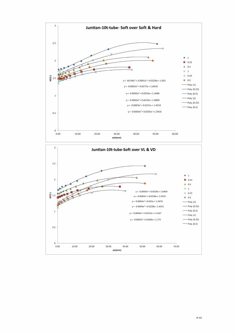
E-43
y = -6E-06x3 + 0.0001x2 + 0.0258x + 1.691
y = -0.0003x2 + 0.0221x + 1.4533
y = -0.0003x2 + 0.0256x + 1.5686
y = -0.0002x2 + 0.0272x + 1.6018
y = -0.0003x2 + 0.0205x + 1.3916
y = -0.0003x2 + 0.0233x + 1.4899
0
0.5
1
1.5
2
2.5
3
0.00 10.00 20.00 30.00 40.00 50.00 60.00
HCF
(-)
set(mm)
Junttan-10t-tube- Soft over Soft & Hard
1
0.25
0.5
1
0.25
0.5
Poly. (1)
Poly. (0.25)
Poly. (0.5)
Poly. (1)
Poly. (0.25)
Poly. (0.5)
y = -0.0003x2 + 0.0329x + 1.6404
y = -0.0004x2 + 0.0228x + 1.4331
y = -0.0003x2 + 0.0258x + 1.5419
y = -0.0003x2 + 0.033x + 1.2676
y = -0.0005x2 + 0.0306x + 1.175
y = -0.0004x2 + 0.0315x + 1.2167
0
0.5
1
1.5
2
2.5
3
0.00 10.00 20.00 30.00 40.00 50.00 60.00 70.00
HCF
(-)
set(mm)
Junttan-10t-tube-Soft over VL & VD
1
0.25
0.5
1
0.25
0.5
Poly. (1)
Poly. (0.25)
Poly. (0.5)
Poly. (1)
Poly. (0.25)
Poly. (0.5)

E-44
y = -5E-07x3 + 2E-05x2 + 0.0043x + 1.2131
y = -2E-06x3 + 0.0001x2 + 0.0011x + 1.1343
y = -8E-07x3 + 3E-05x2 + 0.0036x + 1.1652
y = -6E-07x3 + 2E-05x2 + 0.0058x + 1.2681
y = -2E-05x2 + 0.0038x + 1.1785
y = -5E-07x3 - 7E-06x2 + 0.0055x + 1.2137
0
0.2
0.4
0.6
0.8
1
1.2
1.4
1.6
1.8
0.00 10.00 20.00 30.00 40.00 50.00 60.00 70.00 80.00 90.00 100.00
HCF
(-)
set(mm)
Junttan-10t-tube- VD over Soft & Hard
1
0.25
0.5
1
0.25
0.5
Poly. (1)
Poly. (0.25)
Poly. (0.5)
Poly. (1)
Poly. (0.25)
Poly. (0.5)
0
0.2
0.4
0.6
0.8
1
1.2
1.4
1.6
1.8
2
0.00 10.00 20.00 30.00 40.00 50.00 60.00 70.00 80.00 90.00
HCF
(-)
set(mm)
Junttan-10t-tube- VD over VL & VD
1
0.25
0.5
1
0.25
0.5

E-45
y = -5E-05x2 + 0.0075x + 1.242
y = -3E-05x2 + 0.0045x + 1.1581
y = -5E-05x2 + 0.0064x + 1.1955
y = -0.0002x2 + 0.0206x + 1.2215
y = -0.0002x2 + 0.0147x + 1.1794
y = -0.0002x2 + 0.0203x + 1.1742
0
0.2
0.4
0.6
0.8
1
1.2
1.4
1.6
1.8
2
0.00 10.00 20.00 30.00 40.00 50.00 60.00 70.00 80.00 90.00
HCF
(-)
set(m)
Junttan-10t-tube- VL over Soft & Hard
1
0.25
0.5
1
0.25
0.5
Poly. (1)
Poly. (0.25)
Poly. (0.5)
Poly. (1)
Poly. (0.25)
Poly. (0.5)
y = -0.0001x2 + 0.0136x + 1.2231
y = -0.0001x2 + 0.0106x + 1.1531
y = -0.0001x2 + 0.0128x + 1.18
y = -0.0003x2 + 0.0351x + 1.1429
y = -0.0005x2 + 0.0308x + 1.1185
y = -0.0004x2 + 0.0334x + 1.133
0
0.5
1
1.5
2
2.5
0.00 10.00 20.00 30.00 40.00 50.00 60.00 70.00 80.00
HCF
(-)
set(mm)
Junttan-10t-tube- VL over VL & VD
1
0.25
0.5
1
0.25
0.5
Poly. (1)
Poly. (0.25)
Poly. (0.5)
Poly. (1)
Poly. (0.25)
Poly. (0.5)

E-46
0
0.5
1
1.5
2
2.5
3
0.00 5.00 10.00 15.00 20.00 25.00 30.00 35.00 40.00 45.00
HCF
(-)
set(mm)
Junttan-3t-tube- Hard over Soft & Hard
1
0.25
0.5
1
0.25
0.5
0
0.5
1
1.5
2
2.5
3
0.00 5.00 10.00 15.00 20.00 25.00 30.00 35.00 40.00 45.00 50.00
HCF
(-)
set(mm)
Junttan-3t-tube- Hard over VL & VD
1
0.25
0.5
1
0.25
0.5

E-47
0
0.5
1
1.5
2
2.5
3
0.00 5.00 10.00 15.00 20.00 25.00 30.00 35.00 40.00 45.00
HCF
(-)
set(mm)
Junttan-3t-tube- Soft over Soft & Hard
1
0.25
0.5
1
0.25
0.5
y = -0.0014x2 + 0.0779x + 1.6829
y = -0.0038x2 + 0.0766x + 1.4765
y = -0.0027x2 + 0.0815x + 1.5658
y = -0.0009x2 + 0.0662x + 1.285
y = -0.0018x2 + 0.0701x + 1.2546
y = -0.0009x2 + 0.0434x + 1.1686
0
0.5
1
1.5
2
2.5
3
0.00 5.00 10.00 15.00 20.00 25.00 30.00 35.00 40.00 45.00 50.00
HCF
(-)
set(mm)
Junttan-3t-tube- Soft over VL & VD
1
0.25
0.5
1
0.5
0.25
Poly. (1)
Poly. (0.25)
Poly. (0.5)
Poly. (1)
Poly. (0.5)
Poly. (0.25)

E-48
0.5
0.7
0.9
1.1
1.3
1.5
1.7
0.00 10.00 20.00 30.00 40.00 50.00 60.00 70.00
HCF
(-)
set(mm)
Junttan-3t-tube- VD over Soft & Hard
1
0.25
0.5
1
0.25
0.5
0.5
0.7
0.9
1.1
1.3
1.5
1.7
1.9
2.1
2.3
0.00 10.00 20.00 30.00 40.00 50.00 60.00 70.00
HCF
(-)
set(mm)
Junttan-3t-tube- VD over VL & VD
1
0.25
0.5
1
0.25
0.5

E-49
0
0.5
1
1.5
2
2.5
0.00 10.00 20.00 30.00 40.00 50.00 60.00 70.00
HCF
(-)
set(mm)
Junttan-3t-tube- VL over Soft & Hard
1
0.25
0.5
1
0.25
0.5
y = -0.001x2 + 0.0703x + 1.1371R² = 0.9836
y = -0.0017x2 + 0.0698x + 1.176
0
0.5
1
1.5
2
2.5
3
0.00 10.00 20.00 30.00 40.00 50.00 60.00 70.00
HCF
(-)
set(mm)
Junttan-3t-tube- VL over VL & VD
1
0.25
0.5
1
0.25
0.5
Poly. (1)
Poly. (0.5)

1
REFERENCES
AbdelSalam, S., S. Sritharan, et al. (2009). "Current design and construction practices of
bridge pile foundations." Geotechnical Special Publication(186): 458-465.
Airhart T.P., Hirsch T.J., et al. (1967). Pile-Soil System Response in Clay as a Function
of Excess Pore Water Pressure and Other Soil Properties. Texas, Texas
Transportation Institute.
Allen T. M. (2005). Development of the WSDOT Pile Driving Formula and Its
Calibration for Load and Resistance Factor Design (LRFD).
Allen T. M. (2007). "Development of New Pile-Driving Formula and Its Calibration for
Load and Resistance Factor Design." Transportation Research Record: Journal of
the Transport Research Board(No.2004): pp20-27.
Alvarez C., Zuckerman B. and Lemke J. (2006). Dynamic Pile Analysis Using CAPWAP
and Multiple Sensors. ASCE GEO Congress, Atlanta, Georgia.
Baker C., Parikh G., et al. (1993). Drilled shafts for bridge foundations, Federal Highway
Administration.
Bernardini G., De Pasquale G., et al. (2007). Microwave interferometer for ambient
vibration measurement on civil engineering structures: 1. Principles of the radar
technique and laboratory tests. EVACES’07 Experimental Vibration Analysis for
Civil Engineering Structures. Porto, Portugal 2007: pp.1-9.
Broms B. (1981). Precast Piling Practice, Thomas Telford.
Broms B. , P.C. Lim (1988). A simple pile driving formula based on stress-wave
measurements. Application of stress-wave theory to piles, 3rd international
conference. Vancouvar, Canada: 591-600.
Bruno, D. and M. F. Randolph (1999). "Dynamic and Static Load Testing of Model Piles
Driven into Dense Sand." Journal of Geotechnical and Geoenvironmental
Engineering 125(11): 988-998.
Bullock P.J., Schmertmann J.H., McVay M.C. and Townsend F.C. (2005). "Side Shear
Setup. I: Test Piles Driven in Florida." Journal of Geotechnical
Geoenvironmental Engineering ASCE vol.131(3): pp292-300.

2
Casagrande A. (1964). "Karl Terzaghi." Geotechnique Vol.14(Issue 1): pp.1-14.
Chellis, R. D. (1951). Pile foundations: theory, design, practice, McGraw-Hill.
Chellis, R. D. (1961). Pile foundations, McGraw-Hill.
Chen D. D. S., Wong I. H. and Toto J. V. (1979). "Field Evaluation of Hammer
Efficiency and Pile Driving Criteria." American Society of Civil Engineers
Proceedings, Journal of the Soil Mechanics and Foundations Division: 64-74.
Chow Y.K., Yu C.L., Wong K.Y. and Lee S.L. (1989). "Relation between Peak Driving
Force and the Bearing Capacity of Driven Piles." Journal of Southeast Asian
Geotechnical Society vol.20(no.2): pp103-109.
Davie J.R., Bell K.R. (1991). A pile relaxation case history. International Conference "
Fondations Profondes". Paris, France: 421-429.
Deeks A.J. (1992). Numerical Analysis of Pile Driving Dynamics. Doctor of Philosophy
PhD, University of Western Australia.
Engel R.L. (1988). "Discussion of Procedures for the Determination of Pile Capacity "
Transportation Research Record, Geotechnical Instrumentation No. 1169: p. 54-
61,(Ohio Department of Transportation ODOT).
F. Tavenas, R. Audy (1972). "Limitations of the Driving Formulas for Predicting the
Bearing Capacities of Piles in Sand." Canadian Geotechnical Journal 9(1): 47-62.
FABER O. and ANDREWS E. S. (1947). "DISCUSSION ON A NEW PILING
FORMULA." Journal of the ICE Volume 28(Issue 8): pp. 422.
FELLENIUS B.H. (1988). Variation of CAPWAP results as a function of the operator.
Proceedings of the Third International Conference on the Application of Stress-
Wave Theory to Piles. Ottawa: pp.814 - 825.
Fischer H.C. (1984). Stree Wave Theory for Pile Driving Application. Second
International Conference on the Application of Stress Wave Theory on Piles,
Stockholm, Sweden, Commission of Pile Research, Royal Swedish Academy of
Engineering Sciences.
Fleming K., Weltman A., et al. (2008). Piling Engineering, Taylor & Francis.
Fragaszy R.J. , Higgins J.D., Argo D.E. (1988). Comparison of Methods for Estimating
Pile Capacity, Washington State Department of Transportation. Research Project
Final Report 2.

3
Fragaszy Richard J. , Argo Douglas, Higgins, Jerry D. (1989). "Comparison of formula
predictions with pile load tests." Transportation Research Record(n 1219): p 1-
12.
Fung W.K., Wong C.T., Wong M.K. (2004). "A study on capacity predictions for driven
piles." Transactions, HKIE Vol 11(Iss.no. 3).
Fung W.K., Wong C.T., Wong M.K. (2005). "Observations on using the energy obtained
from stress-wave measurements in the hiley formula." Transactions Hong Kong
Institution of Engineers v 12(n 4): p 19-22.
Fung W.K., Wong C.T., Wong M.K. (2006). "Discussion on observations on using the
energy obtained from stress-wave measurements in the Hiley formula."
Transactions Hong Kong Institution of Engineers v13(n 2): p 63-64.
Fung W.K., Wong C.T.,Wong M.K. (2006). "Response to discussion by Victor Li and
Joley Lam on observations on using the energy obtained from stress-wave
measurements in the Hiley formula." Transactions Hong Kong Institution of
Engineers v 13(n 2): p 65-69.
Gates, M. (1957). "Empirical Formula for Predicting Pile Bearing Capacity." Civil
Engineering Vol.27(No. 3): pp 65-66.
Goble G.G. and Rausche F. (1970). "Pile Load Test by Impact Driving." Highway
Research Record(No.333).
Goble G.G., Scalan R.H., Tomko J.J. (1967). "Dynamic Studies on the Bearing Capacity
of Piles " Highway Research Record (no.167): pp.46-47.
Goble G.G. & Aboumatar H. (1992). Determination of wave equation soil constants from
the standard penetration test. Application of Stress-Wave Theory to Piles. F. B. J.
Barends. Balkema, Rotterdam: 99-103.
Gozeling F.T.M and Van Der Velde E.G. (1996). Application of stress-wave theory to
piles: test results ; proceedings of the Fourth International Conference on the
Application of Stress-wave Theory to Piles, The Hague, Netherlands, 21-24
September 1992, A.A. Balkema.
Hajduk E., Paikowsky S., Hölscher P., Barends F. (2000). Accelerations of a Driven Pile
and the Surrounding Soil. . Proceedings of the 6th International Conference on
the Applications of Stress-Wave Theory to Piles. J. B. S. Niyama. São Paulo,
Brazil, Balkema, Rotterdam-the Netherlands: 541-548.

4
Hannigan P.J., Goble G.G. , Likins G.E. and F. Rausche. (1998). Design and
Construction of Driven Pile Foundations - Workshop Manual Volumes 1 and 2.
Publication Numbers FHWA-HI-97-013 & 14. Washington, D.C., US
Department of Transportation, Federal Highway Administration. Volume 2.
Hereema E.P. (1979). "Relationships between wall friction, displacement velocity and
horizontal stress in clay and in sand, for pile driveability analysis." GROUND
ENGINEERING Volume: 12(Issue Number: 1): pp. 55-65.
Hertlein B., Davis A., (2006). Nondestructive Testing of Deep Foundations, John Wiley
& Sons.
Hiley A. (1925). "Rational Pile-Driving Formula and its Application in Piling Practice
Explained." Engineering 657(721).
Hiley A. (1930). "Pile Driving Calculations with Notes on Driving Forces and Ground
Resistance." The Structural Engineer Vol.8.
Hirsch T.J. and Samson C.H. Jr (1966). Driving Practices for Prestressed Concrete Piles.
Texas, Texas Transportation Institute.
Ho C.E., Lim C.H. (2004). "Dynamic measurement and analysis of pile driving through
thick soft clay." Geotechnical Special Publication (125): 329-347.
Hölscher, P. (1995). Dynamical Response of Saturated and Dry Soils. Delft, The
Netherlands, Delft University Press.
Hölscher, P., and Barends, F. (1996). In-situ Measurement of Soil-Motion near the Toe of
a Dynamically Loaded Pile. 5th International Conference of the Application of
Stress-Wave Theory to Piles, Orlando, FL
Holscher P. (1995). Dynamic Response of Saturated and Dry Soils. Delft, Netherland,
Delft University Press.
Hussein M.H. (2004). A Brief History of the Apllication of Stress Wave Theory to Piles:
Current Practices and Future Trends in Deep Foundation. Deep Foundations.
IDS (2008). "IBIS-S CONTROLLER v2.0 - User Manual." (MN/2007/024): pp.1-47.
IDS Australia (2009). "Georadar Division - General Presentation Slides." pp.1-147.
Isaac, D. V. (1931). "Reinforced Conckrete Pile Formulae." Transactions, Institute of
Engineers, Australia Vol.12 (no.370): pp.305-324.

5
J.F., P. (1970). MECHANICS OF IMPACT PILE DRIVING. Ph.D., University of
Illinois.
Komurka V. E., A. B. Wanger, et al. (2003). Estimating Soil/Pile Set-up. Prepared for
The Wisconsin Department of Transportation. Wisconsin Highway Research
Program #0092-0014
Liang R. Y. (2003). "New Wave Equation Technique for High Strain Impact Testing of
Driven Piles." Journal of Geotechnical Testing vol.26(no.1): pp.111-117.
Liang R. Y., Zhou J. (1997). "Probability Method Applied to Dynamic Pile-Driving
Control." Journal of Geotechnical Engineering, ASCE Vol 123(No.2): pp137-
144.
Liang, R. Y. (1992). "Determination of wave equation soil parameters using in-situ
testing techniques." Determination of wave equation soil parameters using in-situ
testing techniques: 307.
Liang, R. Y., ,Sheng, Y. J. (1992). "THEORETICAL INTERPRETATION OF SMITH
MODEL PARAMETERS." APPLICATION OF STRESS-WAVE THEORY TO
PILES: 111-116.
Likins G. E. (1988). "The Pile Driving Analyzer: Field Testing and Data Interpretation."
PDA User's Day: Cleveland, OH.
Likins G. E., Hussein M.H. (1988). "A Summary of the Pile Driving Analyzer Capacity
Methods - Past and Present." PDA User's Day: Cleveland, OH.
Likins, G. E. (1994). "Helpful Hints for Field Testing and Data Interpretation Using the
Pile Driving Analyzer." Users Days: Orlando, FL.
Lim C. H., Broms B.B. (1990). "Influence of Pile Driving Hammer Performance on
Driving Criteria." Journal of Southeast Asian Geotechnical Society vol.21(no.1):
pp63-69.
Litkouhi S., Poskitt T.J. (1980). "Damping constants for pile driveability calculations."
Geotechnique vol.30(no.1): pp.77-86.
Long J.H (2002). Resistance Factor for Driven Piling Developed from Load Test
Databases. Internation Deep Foundation Congress Geotech Special Publication
ASCE: 944-960.
Lowery L.L. J r . (1967). Dynamic Behavior of Piling. PhD, Texas A&M University.

6
Lowery L.L. J r ., Finley J.R., et al. (1968). A Comparison of Dynamic Pile Driving
Formulas with the Wave Equation. Texas, Texas Transportation Institute, Texas
A&M University.
Lowery L.L. J r ., Hirsch T.J., et al. (1969). Pile Driving Analysis - State of the Art.
Texas, Texas Transportation Institute.
McVay M. C. and Kuo C. L. (1999). ESTIMATE DAMPING AND QUAKE BY USING
TRADITIONAL SOIL TESTINGS, University of Florida, Department of Civil
Engineering: 1-94.
McVay, M. C., B. Birgisson, et al. (2000). "Load and Resistance Factor Design (LRFD)
for Driven Piles Using Dynamic Methods - A Florida Perspective." Geotechnical
Testing Journal 23(1): 55-66.
Middendorp P. and Verbeek G.E.H. (2005). Thirty Years of Experience with the Wave
Equation Solution Based on the Method of Characteristics Proceedings of the
30th Annual Conference on Deep Foundations, Chicago, Illinois, USA, Deep
Foundation Institute.
Mitchell J.K. (1960). "Fundamental aspects of thixotropy in soils." Journal of Soil
Mechanics and Foundation Division, ASCE Vol.86(No.8M3): p19-52.
Morgano C.M, White B.A. & Allin R.C. (2008). Dynamic testing in sensitive & difficult
soil conditions. Application of Stress Wave Theory to Piles. J. A. Santos. Lisbon:
135-138.
Olsen R., Flaate K. (1967). "Pile Driving Formulas for Friction Piles in Sand." Journal of
Soil Mechanics and Foundation Engineering, JSMFE Vol. 93(SM6): 279-297.
Paikowsky, S. (1984). Use of Dynamic Measurements for Pile Analysis. Including
PDAP-Pile-Driving Analysis Program. Newton, Massachusetts, GZA Inc.
Paikowsky, S. (1995). "Using Dynamic Measurements for the Capacity Evaluation of
Driven Piles. ." Journal of the Boston Society of Civil Engineers Section/ASCE
Vol.10(No. 2): pp. 61-76.
Paikowsky S (2004). Load and Resistance Factor Design (LRFD) for Deep Foundation.
Lowell, Masssachusetts, University of Massachusetts.
Paikowsky, S., and Stenersen, K. (2000). The Performance of the Dynamic Methods,
their Controlling Parameters and Deep Foundation Specifications. Keynote
lecture in Stress Wave 2000, Proceedings of the Sixth International Conference

7
on the Application of Stress-Wave Theory to Piles. a. J. B. S. Niyama. São Paulo,
Brazil, Balkema, Rotterdam-the Netherlands: 281-304.(Paikowsky 1982).
Paikowsky, S. and L. Chernauskas (1996). Soil Inertia and the Use of Pseudo Viscous
Damping Parameters. Proceeding of the 5th International Conference on the
Application of Stress-Wave Theory to Piles. M. H. F.C. Townsend, and M.C.
McVay. Orlando, FL: 203-216.
Paikowsky, S., LaBelle, V., and Hourani, N. (1996). Dynamic Analyses and Time
Dependent Pile Capacity. Proceedings of the 5th International Conference on the
Application of Stress-Wave Theory to Piles. M. H. F.C. Townsend, and M.C.
McVay eds. Orlando, FL: 325-339.
Paikowsky, S., Regan, J., and McDonnell, J. (1994). A Simplified Field Method for
Capacity Evaluation of Driven Piles, FHWA.
Paikowsky S., C.M. Marchionda, C.M. O'Hearn, M.C. Canniff (2009). Developing a
Resistance Factor for Mn/DOT's Pile Driving Formula. Lowell, University of
Massachusetts.
Paikowsky S. and Chernauskas L. (1992). Energy Approach for Capacity Evaluation of
Driven Piles. Proceedings of the 4th International Conference on the Application
of Stress-Wave Theory to Piles. F. B. Barends. The Hague, The Netherlands: pp.
595-601.
Paikowsky S., Hajduk E. (2000). Theoretical Evaluation and Full Scale Field Testing
Examination of Pile Capacity Gain with Time: Research Report submitted to the
Massachusetts Highway Department. Massachusetts-Lowell, MA., University of
Massachusetts-Lowell.
Paikowsky S. and LaBelle V. (1994). Examination of the Energy Approach for Capacity
Evaluation of Driven Piles. Proceedings of the International Conference on
Design and Construction of Deep Foundations, Orlando, FL.
Paikowsky S., LaBelle V. and Mynampaty R. (1995). Static and Dynamic Time
Dependent Pile Behavior: Research Report submitted to the Massachusetts
Highway Department, University of Massachusetts-Lowell, MA.
Paikowsky S.G., Hajduk E.L. (2004). "Design and Construction of Three Instrumented
Test Piles to Examine Time Dependant Pile Capacity Gain." Geotechnical
Testing Journal vol.27(no.6): pp.515-531.

8
Paikowsky, S. G., ,, Hajduk E. L. , et al. (2005). Comparison between Model and Full
Scale Pile Capacity Gain in the Boston Area, ASCE.
Paquet J. (1988). Checking Bearing Capacity by Dynamic Loading - Choice of a Method.
3rd Conference on the Application of Stress Wave Theory on Piles, Ottawa,
Canada.
Pile Dynamics Inc. (2006). CAPWAP Case Pile Wave Analysis Program: Background
Report Manual, Version 2006. Cleveland, Oh.
Pile Dynamics Inc. (PDI) (2005). GRLWEAP Wave equation analysis of pile driving:
Procedures and Models Manual. Cleveland, Oh.
Pile Dynamics Inc.(PDI) (1992). PDA-W Users Manual. Cleveland, Oh.
Poulos H.G. (1989). "Pile Behaviour-theory and application." Geotechnique vol.39(no.3):
pp365-415.
Raamot T. (I967). Analysis of Pile Driving by the Wave Equation. Foundation Facts,
Raymond International Inc. Vol.lIl, No. I: pp10-12.
Randolph M.F., Carter J.P. and Wroth C.P. (1979). "Driven Piles in clay-the effects of
installation and subsequent consolidation." Geotechnique vol.29(no.4): pp361-
393.
Rausche, F., G. Thendean, et al. (1997). Determination of pile driveability and capacity
from penetration tests: volume II: appendixes. McLean, Virginia, USA, United
States. Federal Highway Administration (FHWA). Office of Engineering R and
D: 393.
Rausche, F., G. Thendean, et al. (1997). Determination of pile driveability and capacity
from penetration tests: volume III: literature review, data base and appendixes.
McLean, Virginia, USA, United States. Federal Highway Administration
(FHWA). Office of Engineering R and D: 128.
Rausche, F., G. Thendean, et al. (1997). Determination of pile driveability and capacity
from penetration tests; volume 1: final report. McLean, Virginia, USA, United
States. Federal Highway Administration (FHWA). Office of Engineering R and
D: 204.
Rausche F. (1978). "A Critical Examination of the Wave Equation." Transportation
Research Record No. 665, Bridge Engineering, proceeding of a conference

9
conducted by the Transportation Research Board, September 25-27, 1978.
Volume 2: pp.209-213.
Rausche F. (2000). Pile Driving Equipment: Capabilities and Properties [keynote lecture].
Proceedings of the Sixth International Conference on the Application of Stress-
wave Theory to Piles, São Paulo, Brazil.
Rausche F., G.G. Goble & G. Likins (1985). "Dynamic determination of pile capacity."
Journal of Geotechnical Engineering, ASCE. 111(3): 367-383.
Rausche F., Goble G.G., et al. (1988). Recent WEAP Developments. Third International
Conference on the Application of Stress-Wave Theory to Piles. Ottawa, Canada:
164-173.
Rausche F. and Klesney A. (2007). Hammer Types, Efficiencies and Models in
GRLWEAP. PDCA 11th Annual International Conference and Exposition:
Nashville, TN, Cleveland, Ohio, GRL Engineers Inc.
Rausche F., Liang L., Allin R., Rancman D., (2004). Applications and Correlations of the
Wave Equation Analysis Program GRLWEAP. Proceedings of the Seventh
International Conference on the Application of Stresswave Theory to Piles,
Petaling Jaya, Selangor, Malaysia.
Rausche F., Likins G.E., et al. (1986). The performance of Pile Driving Systems
Inspection Manual. Washington DC, FHWA.
Rausche F., Likins G.E., Goble G.G, Hussein M. (1986). The performance of Pile
Driving Systems.
Rausche F., Webster S., et al. (2009). CAPWAP and Refined Wave Equation Analyses
for Driveability Predictions and Capacity Assesmnet of Offshore Pile
Installations. Proceedings of the ASME 28TH International Conference on
Ocean, Offshore and Arctic Engineering, Honolulu, Hawaii, USA, ASME.
Rausche F., M. F., Goble G. G. (1972). "Soil Resistance Predictions From Pile
Dynamics." Journal of the Soil Mechanics and Foundations Division, American
Society of Civil Engineers. Reprinted in Current Practices and Future Trends in
Deep Foundations, Geotechnical Special Publication No. 125, DiMaggio, J. A.,
and Hussein, M. H., Eds, August, 2004. American Society of Civil Engineers:
Reston, VA; 418-440.
Sakai T., Sawai H. and Shioi Y. (1996). Theoretical Analysis of the Pile Driving
Formula. Proceeding of 5th International Conference on the Application of Stress

10
Wave Theory to Piles. F.C Townsend, M. Hussein and M.C. McVay. Orland, FL:
81-88.
Salgado R. (2006). The Engineering of Foundations, McGraw-Hill Science.
Skov R., Denver H. (1988). Time Dependance of Bearing Capacity of Piles. Proceedings
of the Third International Conference on the Application of Stress-Wave Theory
to Piles. Ottawa, Canada, BiTech Publishers: 879-888.
Smith E.A.L. (1950). Pile Driving Impact. Industrial Computation Seminar. New York,
N.Y., International Business Machine Corp.
Smith E.A.L. (1960). "Pile Driving Analyses by the Wave Equation." Journal of the Soil
Mechanics and Foundation Division, ASCE. Vol. 86(1960): 35-61.
Smith, E. A. L. (1955). "Impact and Longitudinal Wave Transmission." Transactions of
the American Society of Mechanical Engineers: pp 963-973.
Smith, E. A. L. (1957). "What Happens When Hammer Hits Pile." Engineering News
Record: pp 46-48.
Smith, E. A. L. (1962). "Pile-Driving Analysis by the Wave Equation." Transactions of
the American Society of Civil Engineers Vol 127(Part 1): pp 1145-1193.
Soderberg L. O. (1962). "Consolidation Theory Applied to Foundation Pile Time
Effects." Géotechnique Vol.12(Issue 3): pages 217 -225.
Stain R. T. (2005). SIMBAT Dynamic Pile Testing – Results of an Independent Pile
Capacity Prediction Event 30th Annual Conference on Deep Foundations,
Chicago, Illinois, USA.
Stevens R.F. (2000). Pile acceptance based on combined CAPWAP analysis. Proc. Conf.
on Application of Stress-Wave Theory to Piles. Sao Paulo, Brazil, Balkema.
Svinkin M.R., Morgano C.M (1994). Pile Capacity as a Function of Time in Clayey and
Sany Soils. Fifth International Conference and Exhibition on Piling and Deep
Foundations, Belgium.
Svinkin, M. R. (1996). Soil damping in wave equation analysis of pile capacity.
Proceedings of Fifth International Conference on the Application of Stress-Wave
Theory to Piles. M. H. M. M. F. Townsend. Rotterdam, Balkema.
Svinkin, M. R. (2002). "Engineering judgement in determination of pile capacity by
dynamic methods." Geotechnical Special Publication ISSU(116): 898-914.

11
Tavenas F. and Audibert J.M.E. (1977). "Application of the wave equation analysis to
friction piles in sand." Canadian Geotechnical Journal Vol.14: pp.34-51.
Tavenas F. and Audy R. (1972). "Limitations of the Driving Formula for Predicting the
Bearing Capacities of Piles in Sand." Canadian Geotechnical Journal Vol.9:
pp.47-62.
Tejchman, A., , Klos, J. (1984). An example of dynamic formulae determined on the
basis of field tests. Application of Stress-Wave Theory to Piles, Swedish Pile
Commission.
Testconsult Limited. "SIMBAT Test Equipment - Hardware and Software Specification."
www.testconsult.co.uk.
The Wave Equation Page for Piling. (1997). "Efficiency and Energy Transfer in Pile
Driving Systems."
The Wave Equation Page for Piling. (1997). "An Overview of Pile Driving Equipment."
December 1999.
Thompson, C. D. and D. E. Thompson (1985). "Real and Apparent Relaxation of Driven
Piles." Journal of Geotechnical Engineering 111(2): 225-237.
Timoshenko S.P., Goodier J. N. (1951). Theory of Elasticity. New York, McGRaw-Hill
Book Company.
Tomlinson, M. (2001). Foundation Design and Construction.
Triantafyllidis, T. (2001). "On the application of the Hiley formula in driving long piles."
Geotechnique v 51(n 10): p 891-895.
Uto K., Aso T., Tsutsumi and Matsui K., (1981). A New Method for Estimating the
Bearing Capacity of A Cast-In-Place Pile. Application of Stress Wave Theory to
Piles. H. Bredenberg. Balkema/Rotterdam: 345-350.
Uto K., Fuyuki M., Ninomiya K. and Omori H. (1992). New Development of Pile
Driving Management System. Application of Stress Wave Theory to Piles.
Balkema/Rotterdam/Brookfield: 351-356.
Verruijt A. (2005). Waves in Piles. Soil Dynamics. Delft, Delft University of
Technology.
Voitus van Hamme, Jansz J.W., et al. (1975). "Hydroblok and Improved Pile-driving
Analysis." International Civil Engineering Vol.3(no.4): pp167-179.

12
Vulcanhammer Guide to Pile Driving (Vulcan Iron Works Inc.). (2011).
"www.vulcanhammer.info." Retrieved 2010, 2010, from
www.vulcanhammer.info.
Warrington D.C. (1996). Development and Potential of the Wave Equation In Closed
Form as applied to Pile Dynamics. Fifth International Conference on the
Application of Stress-Wave Theory to Piles. Orlando, FL.
Warrington D.C. (1997). Closed Form Solution of the Wave Equation for Piles. Master’s
Thesis, University of Tennessee at Chattanooga.
Whitaker, T. (1970). The Design of Pile Foundation.
Wu A.K.H (1985). "Validity of Smith Model in Pile Driving Analysis." Journal of
Geotechnical Engineering Vol.115(No.9): pp1285-1302.
Yang, L. and R. Liang (2009). "Incorporating setup into load and resistance factor design
of driven piles in sand." Canadian Geotechnical Journal 46(3): 296-305.
Zadroga B., Gwizdala K. (1992). Determination of bearing capacity of piles using
modified Delmag dynamic formula. Application of Stress-Wave Theory to Piles,
Balkema.
Zhang B., Yu X. (Bill), et al. (2009). The Dynamic Components of End Bearing in
Highly Cohesive Clay during Pile Driving Process. ASCE Conf. Proc. M.
Iskander, D. F. Laefer and M. H. Hussein. Orlando, Florida, ASCE. 336.
Zhang L., Shek M.P, Ng M.Y. (2004). Wave Equation Parameters for Long Steel H-Piles
Founded in Decomposed Granite. Proceedings of the Seventh International
Conference on the Application of Stresswave Theory to Piles. Petalling Jaya,
Selangor, Malaysia.
Zhang L.M (2005). "Pile Driving Process Monitoring Based on Field Energy
Measurements." Soil and Foundations - Japanese Geotechnical Society
Vol.45(No.6): pp31-41.
Zhou L. and Lao W. (2006). "Studying of the Dynamic Behavior of Pile Cushioning
Materials in Pile Driving." Journal of Testing and Evaluation vol.34(no.5): pp1-6.